analysis of scheduling and topology-control algorithms for
TRANSCRIPT

Analysis of Scheduling andTopology-Control Algorithms for
Wireless Ad Hoc Networks
Diploma Thesis of
Fabian Fuchs
At the faculty of Computer ScienceInstitute for Theoretical Informatics (ITI)
Reviewer: Prof. Dr. Dorothea WagnerAdvisor: Dipl.-Inform. Markus Völker
October 2011 – March 2012
KIT – University of the State of Baden-Wuerttemberg and National Laboratory of the Helmholtz Association www.kit.edu


Acknowledgement
I would like to thank Prof. Dr. Dorothea Wagner for giving me thepossibility to compile this thesis, and my advisor Markus Volkerfor helpful discussions and his continual support. Also, I would liketo thank everybody who supported me during the last six months.
The Lord has remembered us; he will bless us.
Psalm 115:12
Hiermit versichere ich, dass ich die vorliegende Arbeit selbstandig angefertigt habe undnur die angegebenen Hilfsmittel und Quellen verwendet wurden.
Karlsruhe, den 30. Marz 2012. . . . . . . . . . . . . . . . . . . . . . . . . . . . . . . . . . . . . . . . . . . . . . . . . . . . . . . . . . . . . . . . . . . . . . . . . . . . . . . . . . . . . . . .Ort, Datum (Fabian Fuchs)


v
Abstract
The ubiquity of wireless communication is one of the major innovations of the previousdecades. In recent years especially wireless sensor networks evolved from theoretical consid-eration to practical application. In wireless sensor networks, energy conservation is crucialfor the lifetime of the network. Since communication consumes most of the energy, researchin recent years has focused on achieving more energy-efficient communication. One mecha-nism to improve the efficiency of communication is Time Division Multiple Access (TDMA)scheduling, which can be used to manage the medium access. TDMA schedules divide thetime into time slots and assign those time slots to transmissions. In this thesis we studyTDMA scheduling algorithms that enable efficient simultaneous transmission based on theSignal to Interference and Noise Ratio (SINR) model. In our simulations with the networksimulator ns-3, we compare different SINR models and show that the throughput achievedwith TDMA schedules is considerably higher than the throughput achieved with IEEE802.11a CSMA/CA.
Another mechanism that has been considered in this thesis is topology control. Topologycontrol aims at achieving more efficient communication by selecting communication linksand thus reducing the energy required for transmission and minimizing interference. How-ever, many well-known topology control algorithms have only been analyzed theoretically.We use simulations in ns-3 to study the throughput performance and the energy-efficiencyof several well-known topology control algorithms such as the Yao Graph and XTC amongothers. For wireless communication according to the IEEE 802.11a standard, we observethat the throughput performance depends primarily on the number of hops that are onaverage necessary to transmit packets from one node in the network to another node, andonly secondly on further aspects such as the signal strength of the used communicationlinks (given they are above some threshold). Regarding energy efficiency the results ofour simulations show that for fixed transmission powers the consumed energy is stronglycorrelated to the time needed to finish the transmissions, and to the average length of theselected communication links for variable transmission powers.
v


Contents
1. Introduction 11.1. Related Work . . . . . . . . . . . . . . . . . . . . . . . . . . . . . . . . . . . 2
1.2. Contribution . . . . . . . . . . . . . . . . . . . . . . . . . . . . . . . . . . . 3
1.3. Outline . . . . . . . . . . . . . . . . . . . . . . . . . . . . . . . . . . . . . . 4
2. Preliminaries 52.1. Graphs . . . . . . . . . . . . . . . . . . . . . . . . . . . . . . . . . . . . . . . 5
2.2. Wireless Ad Hoc Networks . . . . . . . . . . . . . . . . . . . . . . . . . . . . 6
2.2.1. Wireless Sensor Networks . . . . . . . . . . . . . . . . . . . . . . . . 7
2.3. Models for Wireless Sensor Networks . . . . . . . . . . . . . . . . . . . . . . 7
2.3.1. Communication Graphs . . . . . . . . . . . . . . . . . . . . . . . . . 8
2.3.2. Signal Propagation and Path loss . . . . . . . . . . . . . . . . . . . . 8
2.3.3. Unit Disk Graph Model . . . . . . . . . . . . . . . . . . . . . . . . . 9
2.3.4. The Quasi Unit Disk Graph Model . . . . . . . . . . . . . . . . . . . 9
2.3.5. Interference and the SINR Model . . . . . . . . . . . . . . . . . . . . 10
2.3.6. Dealing with Interference . . . . . . . . . . . . . . . . . . . . . . . . 11
3. Network Simulator ns-3 133.1. Overview . . . . . . . . . . . . . . . . . . . . . . . . . . . . . . . . . . . . . 13
3.1.1. Organization of ns-3 . . . . . . . . . . . . . . . . . . . . . . . . . . . 14
3.1.2. Programming Idioms in ns-3 . . . . . . . . . . . . . . . . . . . . . . 15
3.1.3. OSI Model in ns-3 . . . . . . . . . . . . . . . . . . . . . . . . . . . . 16
3.2. Modeling Networks in ns-3 . . . . . . . . . . . . . . . . . . . . . . . . . . . . 17
3.3. Wireless Communication via IEEE 802.11 . . . . . . . . . . . . . . . . . . . 18
3.3.1. The IEEE 802.11 Model . . . . . . . . . . . . . . . . . . . . . . . . . 18
3.4. Routing Algorithms . . . . . . . . . . . . . . . . . . . . . . . . . . . . . . . 20
3.4.1. Hop-Minimal and Shortest-Path Routing . . . . . . . . . . . . . . . 20
3.4.2. Optimized Link State Routing (OLSR) . . . . . . . . . . . . . . . . 20
3.4.3. Destination-Sequenced Distance Vector (DSDV) . . . . . . . . . . . 21
3.4.4. Ad-hoc On-demand Distance Vector (AODV) . . . . . . . . . . . . . 21
4. Scheduling 234.1. Introduction . . . . . . . . . . . . . . . . . . . . . . . . . . . . . . . . . . . . 23
4.1.1. SINR-based TDMA Schedules . . . . . . . . . . . . . . . . . . . . . . 23
4.2. Issues regarding a TDMA Simulation in ns-3 . . . . . . . . . . . . . . . . . 25
4.2.1. Integrating TDMA Schedules in ns-3 . . . . . . . . . . . . . . . . . . 25
4.2.2. Link Layer Acknowledgements . . . . . . . . . . . . . . . . . . . . . 26
4.2.3. Simulating TDMA using IEEE 802.11 CSMA/CA . . . . . . . . . . 27
4.3. Algorithms . . . . . . . . . . . . . . . . . . . . . . . . . . . . . . . . . . . . 27
4.3.1. GreedySINR . . . . . . . . . . . . . . . . . . . . . . . . . . . . . . . 27
4.3.2. GreedyBuffer . . . . . . . . . . . . . . . . . . . . . . . . . . . . . . . 28
vii
viii Contents
4.4. Experimental Setup . . . . . . . . . . . . . . . . . . . . . . . . . . . . . . . 28
4.4.1. General Wireless Setup . . . . . . . . . . . . . . . . . . . . . . . . . 28
4.4.2. Scheduling Setup . . . . . . . . . . . . . . . . . . . . . . . . . . . . . 29
4.4.3. Parameters and Modifications . . . . . . . . . . . . . . . . . . . . . . 29
4.4.4. Testing Environment . . . . . . . . . . . . . . . . . . . . . . . . . . . 30
4.5. Experiments . . . . . . . . . . . . . . . . . . . . . . . . . . . . . . . . . . . . 30
4.5.1. Comparing SINR and bi-directional SINR . . . . . . . . . . . . . . . 30
4.5.2. TDMA vs. 802.11 CSMA/CA . . . . . . . . . . . . . . . . . . . . . . 33
4.6. Discussion . . . . . . . . . . . . . . . . . . . . . . . . . . . . . . . . . . . . . 35
5. Topology Control 375.1. Introduction to Topology Control . . . . . . . . . . . . . . . . . . . . . . . . 37
5.2. Algorithms . . . . . . . . . . . . . . . . . . . . . . . . . . . . . . . . . . . . 39
5.2.1. All Links Graph (ALG) . . . . . . . . . . . . . . . . . . . . . . . . . 39
5.2.2. Euclidean Minimum Spanning Tree (EMST) . . . . . . . . . . . . . 40
5.2.3. Relative Neighborhood Graph (RNG) . . . . . . . . . . . . . . . . . 40
5.2.4. XTC . . . . . . . . . . . . . . . . . . . . . . . . . . . . . . . . . . . . 40
5.2.5. Gabriel Graph (GG) . . . . . . . . . . . . . . . . . . . . . . . . . . . 41
5.2.6. Yao Graph (YG) . . . . . . . . . . . . . . . . . . . . . . . . . . . . . 42
5.2.7. Restricted Link Strength Graph (RLS) . . . . . . . . . . . . . . . . . 42
5.2.8. Hop, Distance and Energy Spanner . . . . . . . . . . . . . . . . . . . 43
5.2.9. Visual Comparison . . . . . . . . . . . . . . . . . . . . . . . . . . . . 44
5.3. Simulation Setup . . . . . . . . . . . . . . . . . . . . . . . . . . . . . . . . . 45
5.3.1. Parameters and Modifications . . . . . . . . . . . . . . . . . . . . . . 45
5.3.2. Routing Algorithms and Neighborhood . . . . . . . . . . . . . . . . 47
5.3.3. Test Instances and Testing Environment . . . . . . . . . . . . . . . . 48
5.3.4. A Note on the Throughput . . . . . . . . . . . . . . . . . . . . . . . 49
5.4. Experiments I . . . . . . . . . . . . . . . . . . . . . . . . . . . . . . . . . . . 50
5.4.1. Hop, Distance and Energy Spanner . . . . . . . . . . . . . . . . . . . 50
5.4.2. Restricting the Link Strength . . . . . . . . . . . . . . . . . . . . . . 52
5.4.3. Increasing the Workload . . . . . . . . . . . . . . . . . . . . . . . . . 56
5.4.4. Density . . . . . . . . . . . . . . . . . . . . . . . . . . . . . . . . . . 60
5.4.5. Reducing the Transmission Power . . . . . . . . . . . . . . . . . . . 63
5.5. Topology Control and TDMA Schedules . . . . . . . . . . . . . . . . . . . . 67
5.5.1. Preliminaries, Parameters and Modifications . . . . . . . . . . . . . 68
5.6. Experiments II . . . . . . . . . . . . . . . . . . . . . . . . . . . . . . . . . . 70
5.7. Discussion . . . . . . . . . . . . . . . . . . . . . . . . . . . . . . . . . . . . . 72
6. Conclusion 756.1. Outlook . . . . . . . . . . . . . . . . . . . . . . . . . . . . . . . . . . . . . . 76
7. Deutsche Zusammenfassung 79
A. Appendix 83A.1. Patches to ns-3 . . . . . . . . . . . . . . . . . . . . . . . . . . . . . . . . . . 83
A.2. Additional Figures: TDMA vs. Separate Scheduling . . . . . . . . . . . . . 87
A.3. Additional Figures: Increasing the workload . . . . . . . . . . . . . . . . . . 88
List of Acronyms 89
List of Figures 92
List of Tables 93
viii
Contents ix
List of Algorithms 93
Bibliography 95
ix

1. Introduction
The ubiquity of wireless networks in our every-day life is overwhelming. Wireless networkscannot only be used to conveniently access the internet but they also enable new areas ofapplication. Today, many applications use sensors, often even a network of sensors. Dueto the technical development, sensors can now be equipped with wireless communicationinstead of being connected by wire. A wireless sensor node is a micro-computer featuringsensing functionality in combination with a wireless communication device that may beused to connect with other wireless sensor nodes to a wireless sensor network.
The potential of wireless sensor networks opens interesting new fields of applications.One can, for example, equip each patient and each doctor in a hospital with a sensornode that senses information from the patients and transports them to the doctors or to acentral station. Preferably, this node is small, relatively independent from infrastructureand can be used even if the patient is mobile. Another interesting application is crisismanagement. If the required infrastructure is destructed, a wireless sensor network can beused to communicate, sense critical areas or localize helpers. For an overview of additionalapplications of wireless sensor networks, we refer to [ASSC02, YMG08].
There are various constraints for the design of wireless sensor nodes, many of themdepending on the application. However, there are some constraints that are shared by mostapplications. Nodes are usually not connected to the infrastructure and should thereforeendure as long as possible without recharging. Also, the nodes should be small and lowpriced. Since small and cheap nodes usually are not equipped with a large battery, theused algorithms must ensure to conserve as much energy as possible. Since communicationconsumes a major part of the energy used by a sensor node, it is important to communicateefficiently.
Communication in wireless sensor networks has been a major field in research over thepast years. In this thesis, we focus on scheduling and topology control algorithms. Schedul-ing algorithms compute a schedule that assigns each communication link a specified timein which the link is allowed to communicate. This avoids failures in communication due tointerference and enables energy-efficient sleep and duty cycles. The aim of topology con-trol is, to compute a subset of all possible communication links that allow communicationsuch that energy is conserved and interference is minimized.
Sensor networks can be represented using a graph, which enables the application ofgraph-theoretic algorithms. In order to represent the sensor network as a graph, the sensornodes can be modeled as vertices and possible communication between two sensor nodescan be represented by an edge between the corresponding vertices in the graph. Manytopology control algorithms proposed by algorithm engineers use this representation of
1

2 1. Introduction
sensor networks as a graph. Those topology control algorithms are often based on graphalgorithms such as spanning trees or the Gabriel graph.
It is frequently assumed that interference can be minimized by using a sparse topology.However, this is not necessarily true, since limiting the set of communication links does notautomatically avoid interference on neighbors. To examine how the sparseness as well asother properties such as the vertex degree or spanner properties influence the throughputof the different topologies, we examine some proposed topology control algorithms usingthe well-known network simulator ns-3 in this thesis.
1.1. Related Work
The aim of topology control is, to compute a subset of all possible communication linksthat allow communication such that energy is conserved and interference minimized. Inthe past years, research on topology control often considered topology control separatedfrom other aspects like scheduling or routing. The models that were used are mainly graph-based and feature some well-known graph theoretic algorithms like the minimal spanningtrees [LHS05, KPX07], the Gabriel graph or the Delaunay triangulation [GGH+01]. Alsosome other algorithms have been proposed, among which the most popular ones are XTC[WZ03], Yao graph [Yao82] and cone-based-topology-control [WLBmW01], which is similarto the Yao graph.
It has often been assumed that the sparseness of a graph results in low interferencewithout clear argumentation or proofs. In [BvRWZ04], Burkhart et. al. argument thatinterference is not effectively constrained by most topology control algorithms that wereproposed. Afterwards, interference minimal topologies have been examined for differentinterference metrics in [MNL05, LZLD08, YDE11, LTWL11] and it has been shown thatminimizing the maximum interference is NP-hard for the receiver interference model1
[Buc08]. Very recently, interference and energy minimization have been considered jointlyin [PSB12].
A more practical approach is the k-Neigh, which locally selects neighbors for each nodesuch that the number of neighbors is equal to k [BLRS03].
Since retransmissions because of failures due to interference and listening on the wirelessmedium are energy-consuming, computing TDMA schedules became an important topicin research on wireless sensor networks. Spatial reuse TDMA, which allows more thanone transmission to use the same time slot, additionally aims at minimizing the schedulelength. First theoretical approaches to compute short schedules were mainly graph-based[GH01], and hence do not account for cumulated interference. Since the more realisticSINR model and the geometric Signal to Interference and Noise Ratio (SINRG) modelbecame popular in the theoretic research community, many schedules are computed alongthis interference measure [BBS06a, VKW09]. Unfortunately, scheduling is NP-hard inthe general SINR model and both scheduling using common and variable but boundedtransmission powers are NP-hard in the geometric SINR model [GOW07, VKW09].
As energy conservation is an important matter and both scheduling and topology controlcan improve energy conservation, these problems are also considered jointly in recent years.The first that joined the subjects were ElBatt and Ephremides [EE04] and others followedin recent years [BBS06a, VKW09]. Considering uniform transmission, [GWHW09], a firstnon-trivial approximation algorithms to compute a minimal schedules with an approxima-tion factor of O(log n) has been proposed. In [KV10], Kesselheim and Vocking propose adistributed, randomized algorithm that computes an O(log2 n) schedule. Halldorson andMitra improved this result to O(log n) in [HM11]. Very recently, Kesselheim presented aconstant factor approximation algorithm for the optimal selection of transmissions for oneslot in [Kes11]. This yields an O(log n) approximation for the scheduling problem.
1The receiver interference of a node is the number of transmission ranges it lies in.
2
1.2. Contribution 3
A comparison between graph-based and interference-based TDMA schedules in [GH01]shows that interference-based scheduling can improve network capacity by up to one thirdfor (temporarily) stationary situations. A more general outlook on protocol design beyondgraph-based models, which leads towards the SINR model, finds similar improvementsregarding the throughput of wireless networks [MWW06]. In [Mos06], Moscibroda et al.combine topology control with SINR based TDMA schedules.
An overview on algorithmic problems in wireless sensor networks can be found in[WW07]. For topology control we refer to [San05], while a general overview on wirelesssensor networks can be found in [ASSC02, YMG08].
1.2. ContributionMany existing approaches to the topology control problem have only been analyzed
theoretically. It is often assumed that a low node degree minimizes the interference andthus yields energy-efficient communication. To the best of our knowledge, the performanceof many of these topology control algorithms has not been analyzed and compared usinga network simulator or a real network so far. In Chapter 5, we study the throughputperformance as well as the energy efficiency of some topology control algorithms usingthe network simulator ns-3 to process traffic generated by random (possibly multi-hop)sender-receiver pairs.
Based on this simulation, we found that there is no direct connection between a lownode degree and good performance regarding throughput or energy efficiency. In fact,topologies with a low node degree, like those based on the Euclidean Minimal SpanningTree (EMST) or the XTC algorithms, usually achieve considerably less throughput thandenser topologies. Regarding overall energy consumption for variable transmission powerswe observed that the topologies based on the EMST, the XTC algorithm or an energyspanner achieve the best performance according to our measure.
However, both observations are not necessarily caused by the low node degree since itis due to the shorter edge length of those topologies that the transmission power couldbe reduced considerably. And it is mainly due to the increased number of hops that thethroughput performance decreases.
Regarding absolute throughput performance, we found that different topologies fit bestfor different needs. For dense networks, usually a simple restriction on links up to a spe-cific link strength or topologies such as the Yao graph or a 1.1-distance spanner maximizesthe throughput performance while sparse topologies such as those based on XTC or a 1.1-energy spanner are more robust towards sparse networks and achieve the best performancefor sparse networks in our comparisons.
Regarding energy consumption, the results are similar for fixed transmission powersas the length of the transmissions dominate the energy consumption, while for variabletransmission powers those topologies that use mainly short links dominate as the trans-mission power can be reduced considerably. Namely these topologies are those based onthe EMST, the XTC algorithm and the 1.1-energy spanner.
TDMA scheduling is considered an important mechanism to organize medium accessas well as sleep cycles in wireless sensor networks. By applying TDMA schedules to thetopologies considered, we get an additional criterion to analyze the performance of thetopology control algorithms. As some wireless sensor network applications use TDMAinstead of Carrier Sense Multiple Access with Collision Avoidance (CSMA/CA) to re-duce energy consumption, this is an important metric for the topologies. We observedthat regarding both the throughput performance as well as the energy consumption, therelative performance of the topologies has been similar to the relative performance in CS-MA/CA. A restriction to communication links up to a certain signal strength yields thebest throughput performance for both fixed and variable transmission powers as well asthe best energy efficiency for fixed transmission power, while topologies that restrict on
3
4 1. Introduction
very short links, such as the EMST, the 1.1-energy spanner or the XTC, are the mostenergy efficient for variable transmission powers.
1.3. OutlineThis thesis is organized as follows. In Chapter 2 we introduce basic concepts as well as
notations that are used throughout this thesis. Afterwards, in Chapter 3, we take a closerlook at the network simulator ns-3, which is used for the simulations in this work and givean overview on the IEEE 802.11a standard for wireless communication. Chapter 4 con-siders the problem of TDMA schedules in wireless networks. We describe issues that existregarding using TDMA schedules in ns-3 and propose a solution to these issues. We do alsoconsider differences between TDMA schedules and IEEE 802.11a CSMA/CA and providea simulation-based comparison between TDMA schedules and CSMA/CA regarding thethroughput performance. In Chapter 5 we introduce several quality criteria of topologycontrol as well as various topology control algorithms that are examined in this thesis.We discuss aspects such as the workload, the node density, variable transmission powers,and restrictions regarding the link strength based on simulations conducted with ns-3.We measure the performance of the topologies in terms of throughput and an expectedoverall energy consumption. The topologies are also studied in combination with TDMAschedules. Using only the communication links that are chosen by the topology controlalgorithm, routes for the random sender-receiver pairs are computed. For the links thatare on those routes, a TDMA schedule is computed. The throughput and the energy con-sumption for the transmissions, which are processed according to the computed TDMAschedule, are considered. Finally, a brief conclusion and an outlook on future researchdirections are given in Chapter 6.
4

2. Preliminaries
In this chapter, we introduce some basic concepts and notations that are used throughoutthis thesis. In Section 2.1, we give some notations and definitions for graphs. After-wards, an overview on wireless ad hoc networks and wireless sensor networks is given inSection 2.2.1 and in Section 2.2 respectively. Models that are used to represent wirelesssensor networks such that a mathematical analysis is possible are described in Section 2.3.
2.1. GraphsA graph is an ordered pair G = (V,E) comprising a set V of vertices and a set E ⊂ V ×V
of edges.For a graph G = (V,E), G is said to be directed if the elements of E are ordered pairs,
and is called undirected if such pairs are unordered. Within this thesis, an undirectedgraph is equivalent to a directed graph such that for every edge e = (u, v) ∈ E there existsan edge e′ = (v, u) ∈ E.
Each edge e may be assigned a weight, which is given by w(e). For simplicity wewrite w(u, v) := w((u, v)). In the following definitions, we assume that the weight is theEuclidean distance between the vertices, which is given by d(u, v):
Definition 2.1. Given a graph G = (V,E) and two nodes u, v ∈ V .
• A path from u to v (also called a u-v-path) is a sequence (v0, v1, . . . , vp) of vertices suchthat u = v0,v = vp, and there exists an edge (vi−1, vi) ∈ E for every i ∈ {1, . . . , p}.
• A path from u to v is called simple if no vertices are repeated on the path.
• The length of a path (v0, v1, . . . , vp) is defined as the sum over the weight of the edgeson the path:
len(v0, v1, . . . , vp) :=
p∑i=1
w(vi−1, vi).
• A path (v0 = u, v1, . . . , vp = v) from u to v is called shortest path if there is no path(v′0 = u, v′1, . . . , v
′p = v) from u to v with len(v′0, v
′1, . . . , v
′p) < len(v0, v1, . . . , vp′).
• The distance between two vertices u and v is defined as the length of the shortestpath from u to v or. If no path from u to v exists in G, dist(u, v) :=∞.
• A cycle is a path (v0, v1, . . . , vr) with v0 = vr.
• If we require the path (v0, v1, . . . , vr−1) to be simple, we say (v0, v1, . . . , vr) is a simplecycle.
5
6 2. Preliminaries
Definition 2.2. For a graph G = (V,E),
• G is connected, if for each pair (u, v) ∈ V × V a path from u to v exists.
• G is a tree if G is connected and G has no cycles.
Note that in a tree any two vertices are connected by exactly one shortest path.
2.2. Wireless Ad Hoc NetworksA Wireless Ad Hoc Network (WAHN) consists of so-called nodes: micro-computers that
are able to communicate using a wireless network device. It is characteristic for WAHNsthat nodes can communicate with each other without auxiliary devices such as routers.The nodes do not require previous individual setup, but once they are deployed in theenvironment, they are able to set up the wireless network ad hoc. The most typicalfeatures of WAHNs according to [San05, page 4] are:
• Heterogeneous network: The nodes in the network may be diverse. The only thingthat the nodes must have in common is a wireless communication device, which en-ables them to communicate with other nodes in the network. It may be plain radiocommunication, acoustic signals or wireless communication according to transmis-sion standards such as IEEE 802.11 or IEEE 802.15.4. Using, for example, wirelesscommunication according to IEEE 802.11, devices such as smartphones, laptops,PDAs and others can form a wireless ad hoc network, since these devices usually areequipped with an appropriate communication device.
• Mobility: Usually most of the nodes are mobile, i.e., they move or can be moved.
• Diffuse networks: Wireless ad hoc networks are often scattered over a wide area.Multi-hop communication becomes necessary as the span of the network exceeds thetransmission range. This is commonly assumed in applications and hence multi-hopcommunication must be realized.
A considerable amount of researchers have been attracted by WAHNs over the past fewyears. Nowadays the basic technology is available and there are algorithms for manyproblems. Still there are only few applications (for some, see [YMG08]). This is also dueto the fact that although a lot of challenges have been tackled in the past few years, manyof them are still not solved sufficiently. According to [San05, page 8], the main challengesare:
• Energy conservation: Due to mobility and the lack of infrastructure, nodes are usu-ally battery equipped. Nodes should be handy and affordable, therefore the batterysize is rather limited and the available amount of energy must be used as efficientlyas possible.
• Changing topology: Nodes may move or power-down, hence communication partnersmay no longer be reached on the same route as before. Maintaining a correct andefficient topology in mobile networks is a complex task.
• Low-quality communications: In comparison with wired communication, wirelesscommunication is error-prone. Since shadowing, fading, weather conditions and in-terference from other systems influence the communication, considering all factorsrequires sophisticated models.
• Resource-constrained computation: As mentioned, the nodes should be handy, af-fordable and energy efficient. This implies that the computational resources as wellas network bandwidth are scarce.
6

2.3. Models for Wireless Sensor Networks 7
• Scalability: For applications like vehicular networks or crisis-management networks,wireless ad hoc networks must span over large distances and the network may consistof hundreds or even thousands of nodes. Therefore, protocols and algorithms mustscale efficiently up to very large networks.
The main aspects are that the nodes of a wireless ad hoc network must be cheap and aslong-lasting as possible. Thus, minimizing the energy consumption is critical. However,energy is consumed in various ways:
• If the node is turned on, its components need energy to run. Sending componentsto sleep mode or disabling them is preferred.
• The more complex (and hence time-intensive) calculations are, the more energy theyneed. The CPU uses sleep or energy-saving modes to conserve energy if there are nocalculations to be done.
• The communication device uses most energy in transmission mode. This may be upto two thirds of the total power needed by the node according to [San05, page 22].Minimizing the number of transmissions as well as using sleep modes for the networkdevice is vital for long lasting devices.
Depending on the application, one possibly can restrict to relatively low energy levels.But since there is a task that needs to be done, energy must be consumed. To chooseand eventually tailor the algorithms used for this task is a key to minimize the energyconsumption.
2.2.1. Wireless Sensor NetworksOne of the main applications for wireless ad hoc networks are wireless sensor networks.
Sensor networks do not have to be wireless. In fact, there are many applications for wiredsensor networks, such as manufacturing machines, auto mobiles and security systems inbuildings. As wireless technology became popular, applications for wireless sensor networksarose. The technology from wireless (ad hoc) networks has been merged with sensorfunctionality.
Most challenges of wireless ad hoc networks apply for wireless sensor networks, sincethe objectives regarding price, efficiency and persistence are similar. Depending on theactual application, the focus may shift to a subset of the objectives or other objectives andrestrictions may be added. For some wireless sensor network applications, reliability andbalance are essential: If the only sensor that detects a critical situation is powered-downdue to an unbalanced workload, the whole sensor network may be useless. If, on the otherhand, only an average temperature is to be measured, the network can easily cope withan outage or disconnection of smaller parts of the network.
In this thesis, we focus on algorithms for wireless sensor networks. Due to the similarities,our results are mostly applicable for both wireless sensor networks and wireless ad hocnetworks. In Chapter 4 and Chapter 5, we study algorithms for scheduling and topologycontrol, based on simulations using the network simulator ns-3 (see Chapter 3). Thesimulation results do not only tackle more theoretical questions, but they may also beused to chose the algorithms that fit best the application at hand.
2.3. Models for Wireless Sensor NetworksDue to the complexity of wireless communication concerning signal propagation and
interference, researchers in algorithms for wireless sensor networks usually restrict to sim-plified models of the reality. This abstraction leads to mathematical models that enablea mathematical analysis of algorithms that are based on these models. However, due tothe abstraction and simplification, it has to be ensured that good results for the modelscorrelate to good results for real world applications.
7

8 2. Preliminaries
In this section, we first describe models that are used to represent possible communica-tion links between sensor nodes and afterwards introduce models concerning the interfer-ence of transmissions.
2.3.1. Communication Graphs
The topology of wireless networks can be represented with a graph: The nodes in thenetwork correspond to the vertices in the graph, and connection links in the networkcorrespond to edges between the corresponding vertices of the graph. We call this graphthe Communication Graph. A weight can be associated to the edges, this may be thedistance between the nodes, the energy used to communicate over this link, or the averagesignal strength achieved with this link.
Since signal propagation and the reception of a signal are non-trivial, there are variouspossibilities to model the correspondence between connection links in the network andedges in the graph. There are two models that are actively used to model wireless networksin the plane: Unit Disk Graphs and Quasi-Unit Disk Graphs. These models and modelsthat are not restricted to the plane can also be found in [WW07].
Modeling a wireless ad hoc network using a graph is intuitive and allows to utilizeknowledge from centuries of research undertaken within graph theory. There is a widevariety of algorithms for graphs available, hence numerous algorithms can be applied towireless ad hoc networks. But since those algorithms assume a stable communicationgraph, an abstraction from the complexity of wireless signal propagation and reception isneeded.
We consider propagation and path loss in more detail before describing models thatdecide whether an edge between two vertices should be added or not using the Unit DiskGraph and the Quasi Unit Disk Graph models.
2.3.2. Signal Propagation and Path loss
For both wired and wireless communication, the signal propagates along the usedmedium. Other than in wired communication using coaxial or fiber cable, where predictionof the strength and reach of a signal is easy, signal propagation for wireless communica-tion depends on many factors: terrain, atmospheric conditions, weather conditions, andobstacles, among others.
Using the air as a medium, the main influence is the free-space loss of the signal as itpropagates. At distance d to a sender sending with power P, a signal strength proportionalto P /d2 can be observed under ideal conditions. This is due to the fact that the energy ofthe signal distributes equally on the surface of a sphere that originates at the sender andgrows with the speed of light.
As the energy density (or signal strength) decreases with the distance from the sender,three different ranges of the signal can be identified. The first one is the transmissionrange, within which the signal can be received with an error rate that can be compensated.Second, the sensing range, where the receiver can detect that the sender is sending but itis not able to decode the data. The last range is the interference range, where receivers cannot detect that the sender is sending but other signals can be interfered by the sender’ssignal. We further introduce interference in Section 2.3.5.
The energy lost due to signal propagation and obstacles is often called path loss. Usinga log-distance model, the path loss LdB(d) at distance d is modeled in dB1:
LdB(d) = LdB(d0) + 10α log(d/d0),
where α is the attenuation coefficient, which is usually assumed to be about 2 for free spacepropagation and between 3 and 5 for propagation in buildings. The path loss LdB(d0) at
1In this thesis, we use dB for the ratio of two powers and dBm for absolute powers. An absolute power pin milliwatt equals 10 log10(p/1mW ) dBm.
8
2.3. Models for Wireless Sensor Networks 9
reference distance d0 is a hardware dependent constants. The power PdBr(d) that is
received from a receiver at distance d is (in dBm):
PdBmr(d) = PdBm
t−LdB(d)
where PdBmt is the transmission power of the sending node in dBm. Alternatively, the
power Pu(v) received at node v from sender u can be given in watt for d ≥ d0:
Pu(v) = a · Pu(u)
dist(u, v)α(2.1)
where a is a hardware dependent constant and Pu(u) is defined as the transmission powerof node u.
In reality, the path loss is not solely caused by the diffusion of the radio signals, but alsoby reflections on the ground and on obstacles, shadowing (e.g., by obstacles) of potentialreceivers, scattering and diffraction as well as so-called small scale fading.
Clearly, the signal propagation, is responsible for the general trend that the signalstrength decreases with the distance. Shadowing, reflections, scattering and diffractionon the ground or on obstacles may cause worse received signal strengths for nodes thatare, for example, in the shadow of objects that cause reflections.
Using a higher attenuation coefficient, this simple propagation model based on attenu-ation can be adapted to a lossier environment, e.g., one with more obstacles. The detailsregarding the path loss model are according to [WW07, page 28], while more on the fun-damentals on wireless communication can be found in [Gar07].
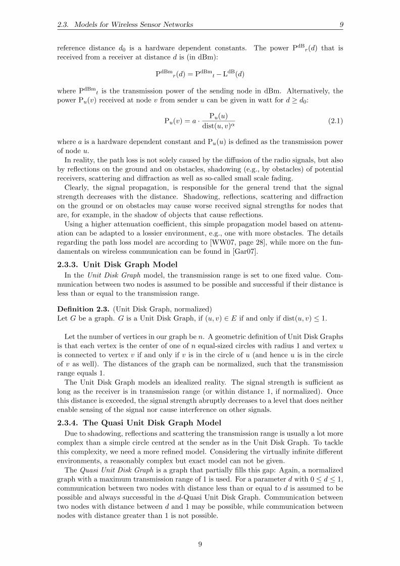
2.3.3. Unit Disk Graph Model
In the Unit Disk Graph model, the transmission range is set to one fixed value. Com-munication between two nodes is assumed to be possible and successful if their distance isless than or equal to the transmission range.
Definition 2.3. (Unit Disk Graph, normalized)Let G be a graph. G is a Unit Disk Graph, if (u, v) ∈ E if and only if dist(u, v) ≤ 1.
Let the number of vertices in our graph be n. A geometric definition of Unit Disk Graphsis that each vertex is the center of one of n equal-sized circles with radius 1 and vertex uis connected to vertex v if and only if v is in the circle of u (and hence u is in the circleof v as well). The distances of the graph can be normalized, such that the transmissionrange equals 1.
The Unit Disk Graph models an idealized reality. The signal strength is sufficient aslong as the receiver is in transmission range (or within distance 1, if normalized). Oncethis distance is exceeded, the signal strength abruptly decreases to a level that does neitherenable sensing of the signal nor cause interference on other signals.
2.3.4. The Quasi Unit Disk Graph Model
Due to shadowing, reflections and scattering the transmission range is usually a lot morecomplex than a simple circle centred at the sender as in the Unit Disk Graph. To tacklethis complexity, we need a more refined model. Considering the virtually infinite differentenvironments, a reasonably complex but exact model can not be given.
The Quasi Unit Disk Graph is a graph that partially fills this gap: Again, a normalizedgraph with a maximum transmission range of 1 is used. For a parameter d with 0 ≤ d ≤ 1,communication between two nodes with distance less than or equal to d is assumed to bepossible and always successful in the d-Quasi Unit Disk Graph. Communication betweentwo nodes with distance between d and 1 may be possible, while communication betweennodes with distance greater than 1 is not possible.
9

10 2. Preliminaries
Definition 2.4. (Quasi Unit Disk Graph, normalized)Let d be a parameter with 0 ≤ d ≤ 1 and G = (V,E) be a graph. G is a d-Quasi UnitDisk Graph, if dist(u, v) ≤ d implies (u, v) ∈ E and dist(u, v) > 1 implies (u, v) 6∈ E.
For the algorithmic models considered in this thesis, subgraphs of the Unit Disk Graphare considered. This is sufficient for our experiments, since—as in reality—successfultransmission can not be guaranteed even for links that are in the Unit Disk Graph. Anexample of unit disks and quasi-unit disks can be seen in Figure 2.1.
Transmission range
AB
C
(a) Unit disks
B
C
A
max. transmission range
min. transmission range
(b) Quasi-unit disks
Figure 2.1.: For the unit disks on the left, the transmission range is depicted by theblack circles. Node B can communicate with node C and vice versa, node A can notcommunicate with any other node. In the Unit Disk Graph, an edge would be addedbetween B and C.For the quasi-unit disks on the right, the communication between B and C is possibleand communication betwen A and B may be possible. For nodes that are not in thegrey circle of a node, communication between those nodes is not possible. In theQuasi-Unit Disk Graph, there would be an edge between B and C, there may be anedge between A and B, and an edge between A and C is not allowed.
2.3.5. Interference and the SINR ModelThe models introduced in the previous section assume that communication is possible
if the receiver is within a certain transmission range of the sender. But this is only oneaspect of physical reception, since it does not only depend on the signal strength of anincoming packet but on the ratio of this signal’s strength to the combined strength ofother signals affecting the receiver to decide if reception of a packet is possible or not.Signals from other simultaneously sending nodes that are not desired at this receiver arecalled interference. Signals originating from the atmosphere and the electronic circuit atthe receiver are called noise.
A relatively easy, graph-based approach to this problem is the construction of a conflictgraph. In such a conflict graph Gconflict, for each communication link in the originalgraph a vertex e is added. An edge ec between two vertices e and c in the conflict graphGconflict is added, if simultaneous transmission on the corresponding communication linksis impossible. A set of transmissions is illustrated in Figure 2.2(a) and the correspondingconflict graph is given in Figure 2.2(b)
The conflict graph does account for noise and interference from individual transmission,but it fails to account for the summed interference of several simultaneous transmissions.Therefore, in the model interference is only a local phenomenon. In reality many interferingsignals even far away add up and may prevent a transmission.
The so-called Signal to Interference and Noise Ratio (SINR) is not based on conflictgraphs, but solely on the fading of the signals. At a receiving node r, the signal power
10

2.3. Models for Wireless Sensor Networks 11
Figure 2.2.: On the left is a set of transmissions. On the right the correspondingconflict graph for a SINR threshold of β = 10. Each transmission pair in the leftpicture is displayed as a vertex on the right.
Ps(r) of the desired signal from node s is called the signal. The ratio of this signal dividedby the noise N and the sum over the interference from all other nodes is the SINR as givenin Equation (2.2).
Ps(r)
N +∑
v∈V \{s} Pv(r)≥ β (2.2)
The SINR model is also called the physical model and it is believed to resemble realityclosely [WW07]. Due to the limitations of conflict graphs, research has lately focused onthe SINR model.
It is not specified in the SINR model how the reception power Ps(r) is determined. Inthe geometric SINR model, SINRG, the power is calculated as a function of the distance:
Pgs(r) := a · Ps(s)
d(s, r)α
with a hardware dependent constant a and the attenuation coefficient α depending onenvironmental factors. d(s, r) is the Euclidean distance from s to r.
2.3.6. Dealing with InterferenceWe do now have a model that describes whether a reception is possible or not given
the interference on the receiver during reception. Unfortunately, it is often unknown inadvance, if and how much interference will occur, since it is unknown to the individualnodes when other nodes will start sending.
According to the OSI model2, the Medium Access Control (MAC) layer handles accessto the medium. In the MAC layer of wireless network devices, similar to wired Ether-net, usually Carrier Sense Multiple Access (CSMA) is used. Other than wired networks,wireless networks use CSMA/CA with collision avoidance instead of collision detection.A wireless sender is, due to its own signal, hardly capable of detecting another nodestransmission while it is transmitting a packet and hence collisions can not be detected.Therefore, it tries to avoid a collision, either by sending Request to Send (RTS)/Clear toSend (CTS) messages or by simply monitoring whether the medium is free for a randomlyspecified time before sending. If the signal of another node is received, after sending a RTSmessage or while monitoring the medium, the transmission is postponed [IEE07, page 256].CSMA/CA is able to avoid most interference, but still there are two cases of sub-optimal
2A brief overview on the lower levels of the Open Systems Interconnection (OSI) model is given when thenetwork simulator ns-3 is introduced in Section 3.1.3.
11

12 2. Preliminaries
behavior that may occur. For both, a setup of 3 nodes is needed: A, B and C.In the so-called hidden station scenario, A sends to B, while C is out of range of A but
B is in range of C. C does not receive the signal of A’s transmission and therefore maystart a transmission. This however leads to interference at B, such that B may not be ableto receive the correct signal from A.
The exposed station scenario is that A transmits data to B, and C receives the signalof A, but B would not receive C’s signal if it would send. Here, C would not send eventhough it would not interfere with B receiving A’s message.
For most use-cases, CSMA/CA is sufficient to avoid interference. In wireless sensor net-works however, there may be a superior solution: Time Division Multiple Access (TDMA)schedules. TDMA manages the medium access by dividing the time in time slots andassigning those time slots to nodes that are allowed to send for the duration of the timeslot. TDMA schedules require the nodes to send data only in time slots they are assignedto. This enables nodes to use the time slots they are not assigned to, to conserve energyby using sleep modes. Also, interference can be minimized, by computing time schedulessuch that the simultaneous transmissions keep interference on a low level. In Chapter 4,we consider TDMA schedules that compute schedules with low interference for wirelesssensor networks.
12

3. Network Simulator ns-3
ns-3 is a time-discrete, event-driven network simulator, which is mainly developed fornetworking research purposes. ns-3’s development initially began in 2006, while its firststable release was in June 2008. Since then, quarterly releases have been made. Thecurrent release is ns-3.13 [ns311a], which has been released on December 23, 2011.
In the following section, we give a brief historic background of ns-3 as well as an overviewover the simulator in general. Afterwards, we briefly introduce the most important modelsfor network modeling in ns-3 in Section 3.2. In Section 3.3, we introduce the IEEE 802.11model implemented in ns-3 as well as a general setup for wireless networks. In Section 3.4,the routing algorithms for wireless networks that are implemented in ns-3 and used inChapter 5 are described.
The ns-3 specific information in this chapter is based on the ns-3 manual [ns311b] andthe documentation delivered with ns-3 itself (mostly the model library or the doxygendocumentation) [ns311a].
3.1. Overviewns-3 is partially based on several predecessors, using models and implementations from
ns-2 [ns211], Georgia Tech Network Simulator (GTNetS) [gtn08] and Yet Another NetworkSimulator (YANS) [LH06]. As the name implies, it is designed to replace ns-2. Hence, inns-3 several issues of the predecessor(s) were addressed:
Coding Style: At the time when ns-2 was developed, the Standard Template Library(STL) as well as other modern software engineering techniques have not been popular oravailable. ns-3 however uses state of the art software engineering as well as several designpatterns, such as smart pointers, templates, callbacks and object aggregation.
Scripting Language: To avoid recompilations of the C++ code, and to provide apotentially easier scripting language to set up simulations, ns-2 is not solely written inC++ but makes heavy use of the scripting language OTcl. Nowadays, students are mostlyunfamiliar to OTcl and it has been reportedly hard to debug the mixture of C++ andOTcl. Therefore, ns-3 uses pure C++ for the core and the models, while offering pythonbindings to set up simulations.
Code Contribution: Hundreds of models have been implemented in ns-2, but neithera coding standard nor consistent software testing or model verification have been enforced.This led ns-3 developers to abandon backward compatibility after careful consideration.Furthermore, a coding standard and code review for code contributions are enforced, anda test infrastructure has been established. This yields code contributions that are far morepromising to be maintained even after the initial author(s) lost interest.
For a more detailed list and along with detailed motivations, we refer to [HLR08].
13

14 3. Network Simulator ns-3
Over the years, many improvements have been made to ns-3 and additional modelshave been implemented (e.g., Internet Protocol Version 6 (IPv6) support, an Instituteof Electrical and Electronics Engineers (IEEE) 802.16 Worldwide Interoperability for Mi-crowave Access (WiMAX) module, etc.). Today, ns-3 is a well equipped network simulatorthat is maintained actively and implements a variety of different models. The most crit-ical ones, like wireless models, have been tested and verified by the research community[PH09, PH10]. In most cases, those models are compatible and can be used in the mainrelease. ns-2, in contrast, has some models that are still missing or under developmentfor ns-3, though many of them are scattered among incompatible branches. One of themodels, which is available in ns-2 but still under development for ns-3, is for example animplementation of IEEE 802.11.4, specifically IPv6 over low power WPAN (6LoWPAN).
Finally, ns-3 is developed as free software, licensed under the GNU GPL version 2license. It is designed to run on Unix- and Linux-based systems. It is possible to run ns-3on Windows using Cygwin. The recent stable release or the development trunk can bedownloaded from the ns-3 homepage [ns311a].
3.1.1. Organization of ns-3
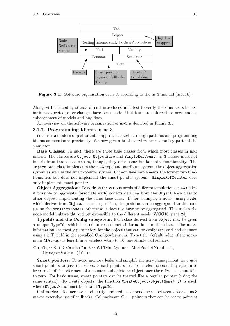
The organization of the ns-3 code can be divided into three parts. The first part is thecore and commonly used parts of the simulator like packets and the event scheduler. Thesecond part consists of the models that are used and needed for network simulation and thethird part are auxiliary helper functions to simplify setting up a simulation environmentand tests to ensure correct functionality throughout version updates.
Main parts of the core are defined by the modern object oriented approach of ns-3. Wegive more information on the main programming idioms, like callbacks and object aggre-gation, in the next section. ns-3, by default, features an event-driven simulator, whichschedules the events according to its 64-bit internal simulation clock. A distributed simu-lator or a real-time simulator can be used instead, if the simulation is to be distributed onseveral machines or integrated into a testbed or virtual machine environment respectively.
Regarding the performance, maintenance and extensibility of a network simulator, pack-ets are crucial. According to Section 16.1 in the ns-3 Model Library [ns311a], the designof the packets for ns-3 was focused on
(a) easy integration in real-world code and systems.
(b) fragmentation and concatenation should be supported.
(c) efficient memory management of packets.
(d) changes in the core of the simulator should not be necessary for the introduction ofnew packets, headers or tags.
The core of the simulator is the most stable part, as it is designed such that new simulationrequirements should not imply changes in the core and the simulator.
The second part consists of some basic models and the models that are needed and hencecontributed by the research community. This part holds models for computers, so-callednodes, from the network device down to the physical layer. It also holds applications androuting algorithms along with other models.
To simplify access to the variety of models, some commonly used models are equippedwith so-called helpers. These helpers make it easy to connect objects. For example,a helper can be used to equip a container of nodes with network devices, or to installwireless communication devices including the MAC, physical and channel layer with cor-responding parameters on several network devices at once. These helpers are defined foruse in simulation scripts. Within the simulator itself, the use of helpers is not allowed.
14
3.1. Overview 15
Test
Helpers
Routing Internet stack Devices Applications
Node Mobility
Common Simulator
Core
Nodes,
NetDevices,
Sockets
Smart pointers,
Logging, Callbacks,
Tracing
Packets Events,
Scheduling
High level
wrappers
Figure 3.1.: Software organisation of ns-3, according to the ns-3 manual [ns311b].
Along with the coding standard, ns-3 introduced unit-test to verify the simulators behav-ior is as expected, after changes have been made. Unit-tests are enforced for new models,enhancement of models and bug-fixes.
An overview on the software organization of ns-3 is depicted in Figure 3.1.
3.1.2. Programming Idioms in ns-3ns-3 uses a modern object-oriented approach as well as design patterns and programming
idioms as mentioned previously. We now give a brief overview over some key parts of thesimulator.
Base Classes: In ns-3, there are three base classes from which most classes in ns-3inherit: The classes are Object, ObjectBase and SimpleRefCount. ns-3 classes must notinherit from those base classes, though, they offer some fundamental functionality. TheObject base class implements the ns-3 type and attribute system, the object aggregationsystem as well as the smart-pointer system. ObjectBase implements the former two func-tionalities but does not implement the smart-pointer system. SimpleRefCounter doesonly implement smart pointers.
Object Aggregation: To address the various needs of different simulations, ns-3 makesit possible to aggregate (associate with) objects deriving from the Object base class toother objects implementing the same base class. If, for example, a node—using Node,which derives from Object—needs a position, the position can be aggregated to the node(using the MobilityModel), otherwise it does not have to be aggregated. This makes thenode model lightweight and yet extensible to the different needs [WGG10, page 24].
TypeIds and the Config subsystem: Each class derived from Object may be givena unique TypeId, which is used to record meta-information for this class. The meta-information are mostly parameters for the object that can be easily accessed and changedusing the TypeId in the so-called Config-subsystem. To set the default value of the maxi-mum MAC-queue length in a wireless setup to 10, one simple call suffices:
Conf ig : : Se tDe fau l t ( ”ns3 : : WifiMacQueue : : MaxPacketNumber ” ,UintegerValue (10) ) ;
Smart pointers: To avoid memory leaks and simplify memory management, ns-3 usessmart pointers to pass references. Smart pointers feature a reference counting system tokeep track of the references of a counter and delete an object once the reference count fallsto zero. For basic usage, smart pointers can be treated like a regular pointer (using thesame syntax). To create objects, the function CreateObject<ObjectName> () is used,where ObjectName must be a valid TypeId.
Callbacks: To increase modularity and reduce dependencies between objects, ns-3makes extensive use of callbacks. Callbacks are C++ pointers that can be set to point at
15

16 3. Network Simulator ns-3
a function which is specified at runtime. The use of callbacks enables ns-3 to dynamicallyconnect objects such that the connection can easily be adapted to other simulation sce-narios. The IP-implementation, for example, is enabled to connect to the layer above byoffering a callback variable that must be set by the layer above. If the TCP protocol setsthe callback to point at TCP, the IP layer is connected to the TCP protocol. However theIP-implementation could just as well be connected to a UDP protocol without adaptingthe IP-implementation - the UDP protocol simply has to make use of the callback designedto connect the IP-implementation with the layer above.
Tracing: Accessing classes and values of each object in the simulator is a complex task.One may want to observe only those packets dropped at the physical layer of a certainnode. Therefore, the object YansWifiPhy implementing the physical layer of this nodemust first be identified using TypeIds and the Attribute System. Then, tracing sourcesdefined at many objects to trace certain values can be used to retrieve the desired values.Here, we install a callback from the trace source PhyRxDrop to a self-defined method thatincrements our counter:
Conf ig : : ConnectWithoutContext ( ”NodeList / [ i ] / Dev i ceL i s t / [ j ] / $ns3 : :Wif iNetDevice /Phy/ $ns3 : : YansWifiPhy/PhyRxDrop” , MakeCallback (&incrementDropCounter ) ) ;
Ways to reach each object and trace sources are given in the ns-3 API documentation.
Random Variables: ns-3 uses the MRG32k3a random number generator by PierreL’Ecuyer. There are several distributions implemented: UniformVariable, NormalVari-able, ErlangVariable and many more. By default, ns-3 gives deterministic results. Arandomization between different runs can be done by using a different seed or differentrun numbers. According to the manual, the ”more statistically rigorous way to configuremultiple independent replications is to use a fixed seed and to advance the run number”[ns311b].
As this gives only a brief introduction to the programming idioms of ns-3, more infor-mation can be found in the ns-3 manual [ns311b].
3.1.3. OSI Model in ns-3
So far, ns-3 implements protocols up to layer 4 of the OSI model. On top of layer 4,there are some applications that can be used to generate and receive traffic. Alternatively,own applications or traffic sources and sinks can be implemented. So far, layer 4 featuresthe Transmission Control Protocol (TCP) and the User Datagram Protocol (UDP) onlyfor Internet Protocol Version 4 (IPv4), though an expansion towards IPv6 is currently inits final stages of being finished.
For communication across the network, ns-3 offers different routing algorithms like globalrouting (which is for wired networks only), Optimized Link State Routing (OLSR), Ad-hocOn-demand Distance Vector (AODV), Destination-Sequenced Distance Vector (DSDV) ora static routing that may be used for user-defined routes. The routing algorithms areexplained in more detail in Section 3.4.
Layer 2 consists of a higher and a lower MAC layer. The higher MAC layer handlesactive probing as well as a packet queue, packet fragmentation and packet retransmissionif needed. The lower MAC layer is mainly responsible for data transmission to the phys-ical layer and basic transactions like acknowledgement of received packets or RTS/CTSmessages.
The physical and channel layer are responsible for the general properties of the usedmedium. Models exist for both wired or wireless communication. This layer includesmodels for propagation loss, propagation delay as well as general error models.
The physical-, channel- and MAC-layer for wireless communication are described inmore detail in Section 3.3.
16

3.2. Modeling Networks in ns-3 17
Applications
Transport protocol
Internet protocol
MAC layer
Physical + Channel
TCP, UDP
IPv4, IPv6
MAC, ARP
Routing protocols: OLSR, DSDV, ...
Interference,
propagation loss
Figure 3.2.: The layers in ns-3 according to the OSI layer model.
3.2. Modeling Networks in ns-3In order to simulate network scenarios, the simulator must provide models of the com-
ponents of the network. In addition to the protocols of OSI layers 1-4, which are brieflydescribed in Section 3.1.3, the following components are most relevant for modeling net-works.
1. A node (Node) can be a network end system such as a personal computer, a networkrouter or, as in our case, a wireless sensor node.
2. Network devices (NetDevice) enable the nodes to communicate. One node can hostseveral network devices. Since every node needs a network device to communicateand via aggregation only one NetDevice could be associated to the node, networkdevices are organized in a list at each node. There are various network device modelsfor the different communication modes, though devices for Ethernet and wirelesscommunication via IEEE 802.11 are most common.
3. The channel (Channel) models the medium between the network devices. It mightbe a wired twisted pair medium, optical fiber, the air for wireless transmission oreven water for underwater acoustic networks.
4. Data transmission is modeled via the transmission of network packets (Packet).Packets usually consist of one or more protocol headers and the actual data, calledpayload. In ns-3, packets are required to be exactly as they are in real networks.
The components given above mostly correspond to base classes of the network simula-tor. There is a wide variety of communication models that implement subclasses of thecomponents given above. There are communication models for
• Long Term Evolution (LTE),
• Underwater Acoustic Network (UAN),
• WiMAX,
• Wireless LAN according to IEEE 802.11 a/b/g/n/e, and
• Ethernet.
Since the general setup is shared among the models, the more detailed view of the wirelessmodel in Section 3.3 gives some reference on how other communication models may be setup. A detailed view on all communication models is given in the ns-3 manual [ns311b] andexamples can be found along with the source code [ns311a].
17

18 3. Network Simulator ns-3
3.3. Wireless Communication via IEEE 802.11The wireless model for ns-3 is based on IEEE 802.11 and offers communication via
802.11a, 802.11b and 802.11g. The physical layer used for wireless communication is basedon the implementation in YANS. The subclasses based on YANS are distinguishable bythe ”Yans” prefix. If there is an ”Yans” implementation of a base class, we use the ”Yans”implementation of the class, since Yans-Wifi is so far the only physical model for wirelesscommunication included in ns-3 by default.
To understand the path each packet takes before, during and after transmission is im-portant for understanding the network simulator as well as the protocols that are used forwireless communication. As it is necessary for our considerations to make and implementsome modifications to the ns-3 code, is inevitable to—at least to some level—understandhow the wireless transmission is defined in the IEEE 802.11a standard and how it is im-plemented in ns-3.
To give insight into how the IEEE 802.11 model implemented in ns-3 works, we firstgive a broad overview and then describe the stations on the path of a packet that is sentfrom one node to another node more detailed.
3.3.1. The IEEE 802.11 ModelThe models used to implement the wireless communication according to IEEE 802.11,
can roughly be assigned to four levels:
• MAC high models, which implement beacon generation, probing and association,
• MAC low models, which implement packet queueing, fragmentation and retransmis-son as well as a Distributed Coordination Function (DCF),
• Rate control algorithms, and the
• Physical layer.
For easier understanding, we try to give the models roughly in the order they affect thepath of a packet that is sent from one node to another node using the wireless communi-cation via IEEE 802.11 in ns-3.
We begin with the WifiNetDevice, as this is the first model which is specific for wirelesscommunication if a packet is sent down from higher layers. The WifiNetDevice holdstogether all objects related to the process of sending and receiving packets using wirelesscommunication: WifiChannel, WifiPhy, WifiMac and WifiRemoteStationManager.
There are three implementations of the models of the higher MAC layer: The ApWifiMacimplements the behavior of a wireless access point. It generates periodic beacons andaccepts association requests. StaWifiMac is the MAC implementation for those stationsthat are not access points (i.e., regular clients). It implements active probing as well asre-association. For ad hoc networks, there is a so-called AdhocWifiMac which does notimplement any beacon generation, probing or association. As the focus of this thesis is onsensor and ad hoc networks, we consider the AdhocWifiMac in the following.
The lower MAC levels consist of a MacLow, which implements functionality for RTS /CTS / ACK transactions. DcfManager and DcfState are used to coordinate access onthe shared medium among the nodes. It relies on CSMA/CA, and optionally RTS/CTSfunctionality. DcaTxop handles packet queuing, fragmentation and retransmissions. It usesDcfManager to decide when a packet can be sent and MacLow to send the packet. To storethe packet until the DcfManager allows the MacLow to send the packet, WifiMacQueue isused.
There are several rate control managers, implementing the base class WifiRemoteSta-
tionManager. Most managers use the SINR of the last packet(s) to decide at which bitratethe next packets should be sent. A manager with a constant bitrate and one with an ide-alized management is also available. As the differences between rate control managers are
18
3.3. Wireless Communication via IEEE 802.11 19
WifiNetDevice
AdhocWifiMac
MacLow
YansWifiPhy
YansWifiChannel
DcaTxOp MacRxMiddle
DcfManager
Listening
Listening
Grant Access
Send(packet)
Enqueue(packet)
Enqueue(packet)
Start
Send
Transmit StartReceive
ReceiveOk
Receive
Receive
ForwardUp
ForwardUp
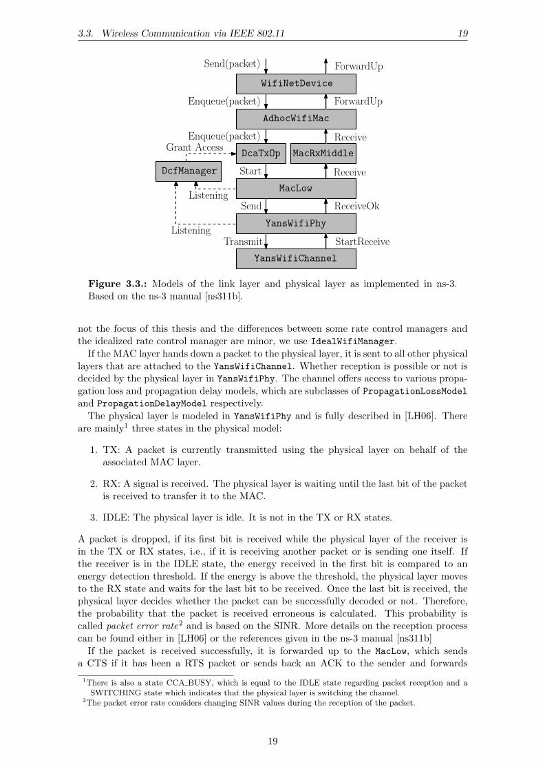
Figure 3.3.: Models of the link layer and physical layer as implemented in ns-3.Based on the ns-3 manual [ns311b].
not the focus of this thesis and the differences between some rate control managers andthe idealized rate control manager are minor, we use IdealWifiManager.
If the MAC layer hands down a packet to the physical layer, it is sent to all other physicallayers that are attached to the YansWifiChannel. Whether reception is possible or not isdecided by the physical layer in YansWifiPhy. The channel offers access to various propa-gation loss and propagation delay models, which are subclasses of PropagationLossModeland PropagationDelayModel respectively.
The physical layer is modeled in YansWifiPhy and is fully described in [LH06]. Thereare mainly1 three states in the physical model:
1. TX: A packet is currently transmitted using the physical layer on behalf of theassociated MAC layer.
2. RX: A signal is received. The physical layer is waiting until the last bit of the packetis received to transfer it to the MAC.
3. IDLE: The physical layer is idle. It is not in the TX or RX states.
A packet is dropped, if its first bit is received while the physical layer of the receiver isin the TX or RX states, i.e., if it is receiving another packet or is sending one itself. Ifthe receiver is in the IDLE state, the energy received in the first bit is compared to anenergy detection threshold. If the energy is above the threshold, the physical layer movesto the RX state and waits for the last bit to be received. Once the last bit is received, thephysical layer decides whether the packet can be successfully decoded or not. Therefore,the probability that the packet is received erroneous is calculated. This probability iscalled packet error rate2 and is based on the SINR. More details on the reception processcan be found either in [LH06] or the references given in the ns-3 manual [ns311b]
If the packet is received successfully, it is forwarded up to the MacLow, which sendsa CTS if it has been a RTS packet or sends back an ACK to the sender and forwards
1There is also a state CCA BUSY, which is equal to the IDLE state regarding packet reception and aSWITCHING state which indicates that the physical layer is switching the channel.
2The packet error rate considers changing SINR values during the reception of the packet.
19
20 3. Network Simulator ns-3
the packet to MacRxMiddle, where duplicates are detected and fragments are recomposed.AdhocWifiMac and WifiNetDevice do simply forward the packet to the layers above.
The physical layer for wireless communication based on YANS is the only model that isdelivered with ns-3 so far. But there exists a so-called PhySim-WiFi model, which modelscertain wireless communication more detailed. Yans-Wifi abstracts from the details ofthe packet transmission by considering only an average signal strength and the length ofthe packet. The Physim-Wifi model goes into the detail of the signal level to computewhether a packet can be received or not. However, the details of the PhySim-Wifi arecoming with an excessively high running time (300 to 40000 times slower than the defaultmodel, depending on path loss and error models) [PMSH10]. Due to this we come to theconclusion that for our needs, the default Yans-Wifi is satisfactory, since the details ofsignal processing are not considered. For our simulations, an average signal strength forthe whole packet is sufficiently detailed.
3.4. Routing Algorithms
In wireless sensor networks, communication between nodes that are not within trans-mission range may be necessary. Hence, the communication must use intermediate nodesthat forward the packet to the receiver. The route that must be taken to reach a cer-tain destination is computed by the routing algorithms. Since multi-hop communicationis considered in Chapter 5, we describe routing algorithms that are implemented in ns-3in this section. Since we consider wireless networks, OLSR, DSDV and AODV as wellas a static routing algorithm are available. Using the static routing algorithm, we imple-mented hop-minimal and shortest-path routing algorithms that are described along withthe algorithms directly implemented in ns-3 in the next sections.
3.4.1. Hop-Minimal and Shortest-Path Routing
Both hop-minimal and shortest-path routing are implemented using the ns-3 Ipv4Static-Routing. Both are very basic routing protocols that do not feature typical options ofrouting algorithms for (mobile) ad hoc networks such as flooding or the evasion of brokenlinks.
Since the static routing algorithm in ns-3 does not offer predefined routes in the wirelessenvironment, the possible routes must be computed and added to the routing protocol.To compute the routes, a simple breadth-first search finds the hop-minimal or the shortestpath to each node respectively. Starting from a source s, for each processed node thealgorithm stores the hop-minimal or shortest node on the (either hop-minimal or shortest)path from the source that led to its processing. This node is used as gateway in the routingalgorithm from the source to the processed node.
3.4.2. Optimized Link State Routing (OLSR)
The OLSR routing protocol is specifically designed for mobile ad hoc networks. It isa proactive routing protocol and hence establishes routes before they are demanded. Tofind its one and two hop neighbors, each node uses OLSR-hello messages. Additionally,each node selects special nodes, so-called multipoint relays such that all one- and two-hopneighbors can be reached through them. Each multipoint relay node does then distributeits neighbor information to the nodes that selected it as a multipoint relay. In contrast tothe classical approach, where each node retransmits each message when it is received thefirst time, this reduces message overhead.
According to RFC 3626 Optimized Link State Routing Protocol (OLSR) [CJ03], OLSRprovides hop-optimal routes and particularly suits large and dense networks. The ns-3implementation of OLSR has been developed for ns-2 and was ported to ns-3. It is mostlycompliant with RFC 3626, except for MAC layer feedback, which is missing in the ns-3implementation of OLSR.
20

3.4. Routing Algorithms 21
3.4.3. Destination-Sequenced Distance Vector (DSDV)DSDV is based on the Bellmann-Ford algorithm [CLRS09, pages 651-655]. DSDV uses
a routing table to keep track of routes to possible destinations and regularly exchangesthese tables with neighbors. One problem that arises in the Bellmann-Ford-based routingalgorithms is the problem of induced routing loops. Considering 3 nodes, A, B and Cwhere A can only communicate with B, B can communicate with A and C, and C canonly communicate with B. If A breaks down, B notices that it can not reach A anymoreas A does not respond. However, B does also receive updates from C which tells B that Ais just 2 hops away from C. This is not anymore true and induces a (temporary) routingloop which lasts (in this case) for another two updates. One of the major achievements ofDSDV is that it avoids this routing loop problem by using incrementing sequence numbersgenerated by the destination node. To update the routes, full or incremental updatesare distributed between nodes. For highly dynamic, long-lasting networks, the graduallyincrementing sequence number may become an issue.
In the ns-3 implementation of DSDV, a node sends out updates on its routing tablewhenever the routing table is changed.
3.4.4. Ad-hoc On-demand Distance Vector (AODV)In contrast to OLSR and DSDV, AODV is a reactive routing protocol, and therefore
discovers routes once they are required. For each neighbor of a node, a list that holdsdestination IPs that are likely to use this neighbor as a next hop towards the destinationis hold. Then, to find a new route, the source node sends out a route request that isforwarded until the target, or a node with a route to the target, is found. Discoveredroutes are stored, but invalidated after a specified time. To avoid the Bellmann-Ford loopproblem, AODV also uses monotonously increasing sequence numbers, which may becomean issue on highly dynamic, long-lasting networks.
The ns-3 implementation of AODV is based on RFC 3561 AODV Routing [PBRD03].Some issues that concern cooperation of OSI layers are claimed to be not described inthe RFC. The ns-3 implementation of AODV hence implements heuristics to (1) detectand avoid unidirectional links (2) use hello messages to detect broken links and (3) detectduplicate packets. For wireless transmission, the use of hello messages is critical, sincethose messages are transmitted using a lower bit rate than usual packets. Therefore, theytravel further and are more resistant to interference.
The performance of AODV-based multi-hop transmission has been relatively poor inour initial experiments. Problems with the implementation of AODV in ns-3 as well as asimilarly performance have also been reported in [NCc+11]. Therefore, we do not considerthe AODV routing algorithm in our experiments in Chapter 5.
21


4. Scheduling
In this chapter we consider scheduling algorithms that compute Time Division MultipleAccess (TDMA) schedules for transmissions such that the transmissions can be processedsimultaneously without failure due to interference.
We will first give an introduction to SINR-based scheduling in the next section. Then,some issues regarding the simulation of TDMA scheduling in the network simulator ns-3are discussed in Section 4.2. An overview on the considered scheduling algorithms is givenin Section 4.3. In Section 4.4, we describe the experimental setup that is used to conductthe experiments. The experiments themselves are described and their results are presentedin Section 4.5. This chapter is concluded with an overview over the results of this chapterin Section 4.6.
4.1. Introduction
TDMA schedules manage medium access by dividing the time into time slots and as-signing these time slots to wireless sensor nodes, which are only allowed to send duringthe assigned time slots. In the assigned time slots, a node may access the medium fortransmission or reception. In time slots the node is not participating, it can use its sleepmodes to conserve energy. Since energy is a very valuable resource for wireless sensornodes, the use of TDMA scheduling is tempting.
4.1.1. SINR-based TDMA Schedules
Before going into the details of TDMA scheduling, we will first introduce some notations:A transmission pair t consists of a sender s and receiver r, t := (s, r), and is associatedwith a specified amount of data that must be transferred. For now, we assume the amountof data to equal the amount of data transferable in one time slot. To compute a schedule,each transmission pair must be assigned one time slot in order to transmit the associateddata.
To achieve schedules such that the interference between the transmission pairs in eachslot is low enough to enable a successful transmission, usually the Signal to Interferenceand Noise Ratio (SINR) model is used. Using the SINR model, we can decide whethera set of transmission pairs can be active in the same time slot (i.e., whether they cantransmit their data simultaneously). The SINR model is introduced in Section 2.3.5. Weassume the SINR threshold β to be given as β = 10 dB in this chapter.
Assume a set S of transmission pairs, such that all senders can transmit their datasimultaneously (i.e., in one time slot) according to the SINR model. Then, we can decidebased on the SINR formula whether a transmission pair t := (s, r) can be processed while
23

24 4. Scheduling
the other pairs in S are transmitting. If it holds that
Ps(r)
N +∑
(s′,r′)∈S Ps′(r)≥ β, (4.1)
r can receive the signal of s with a signal strength that is sufficiently high to decode thesignal, even though the other pairs in S are sending. However, this is not sufficient, sinceit is not clear how t influences the transmissions that are yet in S. Before adding t to S,we have to check for each tj ∈ S whether it can still transmit its data successful accordingto the SINR model while the transmission pairs in S ∪ {t} are transmitting. The notationused in this formula has been introduced in Section 2.3.5. In short: Ps(r) is the energyreceived at node r when s is sending, Ps(s) is defined as the sending power of node s, andN is the background noise induced by the circuit and the environment.
Figure 4.1.: Input and output of the TDMA scheduling problem. On the left is aset of transmissions, i.e. sender-receiver pairs. On the right, a possible assignment fothese transmissions to TDMA time slots is depicted. Each color corresponds to onetime slot.
Sending wireless signals with higher energy increases the energy with which the signalis received at the receiver. Hence, it enables the sender to reach receivers further away. Atthe same time, however, the interference on receivers that are not interested in the signalis increased accordingly. As we want to minimize interference and ultimately conserveenergy, sending with lower power, limits the transmission range while also limiting theinterference on other nodes. Therefore, the lowest possible sending power must be chosensuch that the intended receiver is able to decode the signal according to the SINR equation.
Let T be the set of all transmission pairs. We can now define the TDMA schedulingproblem, which is the problem of finding a slot assignment for each transmission in T suchthat for each transmission in the time slot the SINR equation holds and the total lengthof the schedule is minimal. We call an assignment of transmissions to a time slot suchthat the SINR equation holds for each transmission in the corresponding time slot valid.The definition of the scheduling problem for a common transmission power of all nodes isgiven in Definition 4.1.
Definition 4.1. (TDMA scheduling problem with common transmission power)Given a set of transmissions T with common transmission power P and time slotsS1, S2, . . . , find an assignment of the transmissions in T to time slots Si such that
(a) For each Si: for each t = (s, r) ∈ Si the SINR equation holds, i.e.,
PN +
∑(s′,r′)∈Si\{t}
Ps′ (r)≥ β
24
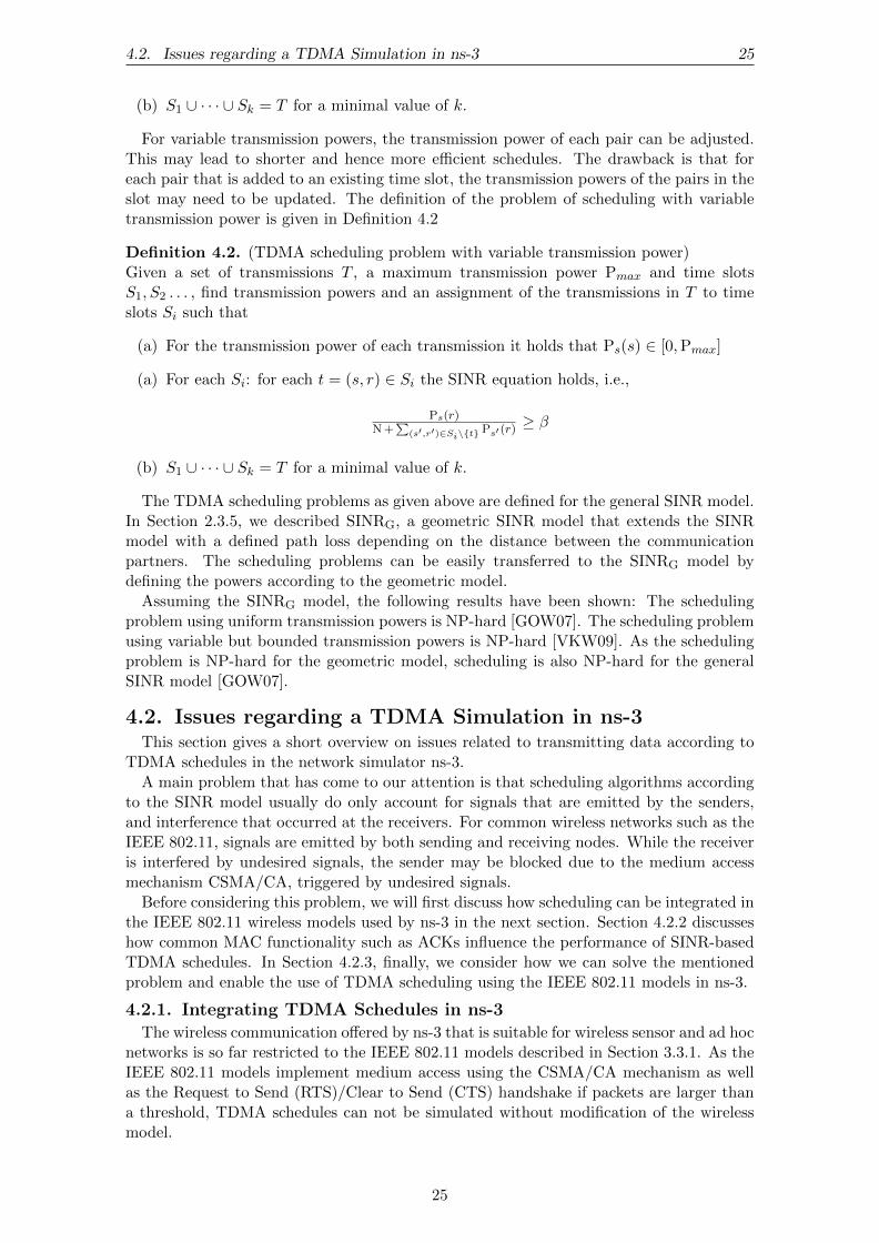
4.2. Issues regarding a TDMA Simulation in ns-3 25
(b) S1 ∪ · · · ∪ Sk = T for a minimal value of k.
For variable transmission powers, the transmission power of each pair can be adjusted.This may lead to shorter and hence more efficient schedules. The drawback is that foreach pair that is added to an existing time slot, the transmission powers of the pairs in theslot may need to be updated. The definition of the problem of scheduling with variabletransmission power is given in Definition 4.2
Definition 4.2. (TDMA scheduling problem with variable transmission power)Given a set of transmissions T , a maximum transmission power Pmax and time slotsS1, S2 . . . , find transmission powers and an assignment of the transmissions in T to timeslots Si such that
(a) For the transmission power of each transmission it holds that Ps(s) ∈ [0,Pmax]
(a) For each Si: for each t = (s, r) ∈ Si the SINR equation holds, i.e.,
Ps(r)N +
∑(s′,r′)∈Si\{t}
Ps′ (r)≥ β
(b) S1 ∪ · · · ∪ Sk = T for a minimal value of k.
The TDMA scheduling problems as given above are defined for the general SINR model.In Section 2.3.5, we described SINRG, a geometric SINR model that extends the SINRmodel with a defined path loss depending on the distance between the communicationpartners. The scheduling problems can be easily transferred to the SINRG model bydefining the powers according to the geometric model.
Assuming the SINRG model, the following results have been shown: The schedulingproblem using uniform transmission powers is NP-hard [GOW07]. The scheduling problemusing variable but bounded transmission powers is NP-hard [VKW09]. As the schedulingproblem is NP-hard for the geometric model, scheduling is also NP-hard for the generalSINR model [GOW07].
4.2. Issues regarding a TDMA Simulation in ns-3This section gives a short overview on issues related to transmitting data according to
TDMA schedules in the network simulator ns-3.A main problem that has come to our attention is that scheduling algorithms according
to the SINR model usually do only account for signals that are emitted by the senders,and interference that occurred at the receivers. For common wireless networks such as theIEEE 802.11, signals are emitted by both sending and receiving nodes. While the receiveris interfered by undesired signals, the sender may be blocked due to the medium accessmechanism CSMA/CA, triggered by undesired signals.
Before considering this problem, we will first discuss how scheduling can be integrated inthe IEEE 802.11 wireless models used by ns-3 in the next section. Section 4.2.2 discusseshow common MAC functionality such as ACKs influence the performance of SINR-basedTDMA schedules. In Section 4.2.3, finally, we consider how we can solve the mentionedproblem and enable the use of TDMA scheduling using the IEEE 802.11 models in ns-3.
4.2.1. Integrating TDMA Schedules in ns-3
The wireless communication offered by ns-3 that is suitable for wireless sensor and ad hocnetworks is so far restricted to the IEEE 802.11 models described in Section 3.3.1. As theIEEE 802.11 models implement medium access using the CSMA/CA mechanism as wellas the Request to Send (RTS)/Clear to Send (CTS) handshake if packets are larger thana threshold, TDMA schedules can not be simulated without modification of the wirelessmodel.
25

26 4. Scheduling
There is a wide consent in the research community that scheduling is usually done in theMAC layer, since it handles access to the medium [ASSC02, YMG08]. In ns-3, however,there is no MAC layer available that enables TDMA scheduling for wireless communication.This due to the fact that medium access using TDMA is not considered in the IEEE 802.11standard.
Since the MAC layer of ns-3 is very detailed (cf. Section 3.3.1) and hence complex, anadaptation of this model without risking undesired behavior was not considered possible.We therefore implemented scheduling using the application layer and adapt the MAC layerto the needs of TDMA scheduling as good as possible.
4.2.2. Link Layer Acknowledgements
Many common MAC protocols rely on bi-directional communication, due to MAC ac-knowledgements (ACKs) and possible RTS/CTS handshakes. RTS/CTS handshakes caneasily be avoided in the wireless model of ns-3 by using packets smaller than 2200 bytes.Since we usually use packets with a payload of 512 bytes, this is not a problem.
The bi-directional communication introduced by link level ACKs however is seldomconsidered in scheduling algorithms. This may be partially due to the fact that common802.11 wireless MAC protocols do not yet offer TDMA scheduling functionality. Anotherreason may be the emergence of wireless communication according the IEEE 802.15.4standard for ”Wireless Personal Area Networks”, namely ZigBee [Erg04] and 6LoWPAN[MKHC07], which are designed for very low bandwidths and low energy consumption.IEEE 802.15.4 does offer both, a slot-based scheduling as well as the ability to disableacknowledgements.
However, for applications that have high demands on the bandwidth, using image orvideo processing for example, such a low bandwidth does not suffice and wireless com-munication using 802.11 or similar standards is required. This requirement is known andvarious MAC protocols have been proposed that fit the needs of wireless sensor and adhoc networks. However, many do still use ACKs [vDL03, SKS06], because without usingACKs the sender can not be sure whether the receiver received the message sent to himor not. Also, ACKs enable the sender to adapt its sending concept according to the ACKsreceived.
Even though ACKs are rather short, they interfere with other packets on a regular basis.Therefore, we need a more general inspection of the SINR constraint for each transmissionthat should be added to a time slot. It must be considered that sending nodes are interferedwhile waiting for a free channel if they receive packets, as well as that receiving nodes areinterfering other nodes by sending ACK messages. We assume that for each transmission,either the sender or the receiver is sending at a time.
To account for those changes, we can use the following rule. If a transmission pair tshould be added to an existing set of simultaneous transmissions S, Equation (4.2) andEquation (4.3) must hold for every pair (s, r) ∈ St := S ∪ {t}.
Ps(r)
N +∑
(s′,r′)∈St\{(s,r)}max(Ps′(r),Pr′(r))≥ β. (4.2)
Pr(s)
N +∑
(s′,r′)∈St\{(s,r)}max(Ps′(s),Pr′(s))≥ β. (4.3)
Note that by the constraints we added, we ensure that the SINR equation holds forboth, receiving and sending nodes. This model has been proposed in [BBS06b]. We callthis model the bi-directional SINR model and the previously introduced model the generalSINR model. This approach can be used for both common or variable transmission powerscheduling.
26

4.3. Algorithms 27
4.2.3. Simulating TDMA using IEEE 802.11 CSMA/CAAs discussed earlier, the IEEE 802.11 models do not implement TDMA but are restricted
to CSMA/CA. Since we do not consider changing large parts of the ns-3 simulator as anoption, we have to adapt the models such that they can be used for TDMA scheduleswithout actually changing their code.
The main difficulty is, to force the sender to ignore the CSMA/CA mechanism and thusto force it to start its transmissions even though it may be reached by packets from othernodes sending simultaneously. For each packet that reaches a node, the energy of thispacket is compared to the energy detection threshold. If the energy is higher than thethreshold, the node tries to receive the packet and notificates the CSMA/CA mechanismthat the medium is used. To avoid these notifications, the energy detection threshold ofthe sending nodes can be increased. However, it can not be set to an arbitrary high level,since ACKs from the receiving node must be received.
Using the bi-directional SINR model, it holds that the energy of all other nodes thatare sending in the same time slot (both sending and receiving nodes) is not larger thanthe signal of the intended partner in the transmission pair. In fact, all interfering signalsreceived at a node are exceeded by the intended signal by a factor of at least β.
Using this knowledge, we set the energy detection threshold such that the signal of thereceiver can be received, but all other incoming signals are not considered. Note thatthis is not according to any standard. It is a workaround to disable CSMA/CA in ns-3.Since messages received at the sender are also not considered by scheduling algorithms,the workaround is acceptable.
Using the general SINR criterion for TDMA schedules, however, there seems to be noway to easily bypass CSMA/CA in ns-3. This is because the interference that affects thesending node is not strictly limited. Since the distance of the sender to another sender maybe arbitrarily small, the signal strength from the interfering sender may be considerablyhigher at the sender than at the receiver.
Another mechanism that hinders TDMA schedules is the RTS/CTS handshake mecha-nism. As mentioned before, RTS/CTS is only used for large packets in ns-3 and hence thishandshake mechanism can be circumvented by using packets with 512 bytes of payload,which is the default size of the used application.
To force the MAC layer to send packets only during the assigned time slot, we needto make sure the MAC layer runs out of packets once the upper layer that implementsTDMA stops sending packets (i.e., the time slot is over). Since modifications on the MAClayer have not been an option, all queues from the application layer to the physical layerhad to be disabled. Since those queues are needed, a small number of packets has beenallowed. For an exact description of the used parameters and modifications, we refer toSection 4.4.3.
4.3. AlgorithmsIn this section we introduce the—rather intuitive—algorithms considered for the schedul-
ing experiments. Due to timely limitations of this thesis we refrained from an extensionon more elaborate scheduling algorithms.
4.3.1. GreedySINRAfter ordering the transmissions according to their link gain (which equals an ordering
according to their distance in the used log-distance model), the algorithm fills one slot ata time. For each new slot, the first transmission that is added is the not yet scheduledtransmission pair with the highest link gain. Then, for each transmission that is not yetscheduled, this transmission is temporarily added to the slot. In this temporary slot, allSINRs are calculated and if all SINRs are above a specified threshold, the worst SINR thatoccurs in this slot is stored. The transmission that yields the largest of these worst SINRvalues is added to the slot. If no transmission fits in the slot, a new slot is added.
27

28 4. Scheduling
The schedule can be computed for both, the SINR model as well as the bi-directionalSINR model using this approach. We call the algorithms GreedySINR (GS) and Greedy-BiSINR (GBS), respectively.
4.3.2. GreedyBuffer
In this algorithm, the transmission pairs are again processed in order of decreasing linkgain and one slot is filled after the other. For each transmission that is temporarily addedto the slot, the buffer, which is the sum of differences between the SINR of each receiverand the SINR threshold, is calculated. The transmission that allows the largest buffer ischosen. If, for a transmission in the temporary time slot, the SINR value is less than thethreshold, this transmission is discarded regardless of the calculated buffer.
We call this algorithm GreedyBuffer (GB) and the one using the bi-directional SINRmodel GreedyBiBuffer (GBB).
4.4. Experimental Setup
In this section, we describe the setup that is used for the scheduling experiments. We willfirst introduce the general wireless setup that is used in our experiments. Afterwards, theassumptions made towards the scheduling algorithms are described in Section 4.4.2. Sec-tion 4.4.3 specifies the modification to ns-3 that were necessary to realize TDMA schedul-ing.
4.4.1. General Wireless Setup
For wireless communication, the IEEE 802.11a standard is used. This allows commu-nication with a data rate of up to (theoretically) 54 Mbit/s in the 5 GHz band. However,communication using high data rates such as 54 Mbit/s requires a higher SINR than com-munication with lower data rates. This is due to the lower redundancy used for high datarates. Since those high data rates can only be achieved for rather local communication,we chose to use a ConstantRateWifiManager that sends the data constantly with a datarate of 24 Mbit/s using the OfdmRate24Mbps data mode. This allows communication overa distance of up to about 45 meters using our log-distance model parameters. To ensurethat communication is possible, we use 40 meters as maximal distance in our experiments.
We use both, the UDP and TCP protocols. As there are various TCP implementa-tions in ns-3 to choose from, we use the TcpNewReno as this is the most contemporaryimplementation.
The propagation loss is modeled according to the log-distance model (LogDistance-PropagationLossModel): L = L0 + 10 · α · log10( dd0 ), where L is the path loss in dB,L0 is the reference path loss at distance d0, α is the attenuation coefficient and d is thedistance between sender and receiver. The parameters used are L0 = 46.6777, d0 = 1α = 3, which corresponds to an average free space environment with some obstacles. Anattenuation coefficient α of 3 rather than 2 has been reported to be more representativeof real environments [BBS06a].
To model the physical medium, the model provided by YansWifiPhyHelper::Default
is used. The wireless net device is configured as an ad hoc station (AdhocWifiMac) withoutQuality of Service (QoS) (NqosWifiMacHelper::Default). Each device is assigned onedistinct IP-Address within the subnet. For our simulation usually less than 255 nodes wereused and therefore the 10.1.1.0/24 subnet was sufficient.
Since mobile nodes have not been considered in our experiments, a constant positionmodel is used (ConstantPositionMobilityModel). Random effects such as shadowing orsmall scale fading (cf. Section 2.3.2) can be realized in ns-3, however, due to the runningtime of simulations with ns-3, which is up to a few hours without such random effects,we refrained from using those models. The introduction of random effect would furtherincrease the number of runs needed for the results to even out sufficiently.
28

4.4. Experimental Setup 29
4.4.2. Scheduling SetupFor a theoretic analysis of scheduling algorithms, usually only the schedule length is
considered. Using only the schedule length, however, is not practical for a simulation-based analysis. If one transmission did not finish in one time slot but has almost finished,accounting for another time slot is not fair. However, since we had to fall back on higherprotocols to implement TDMA schedules, very small time slots are not possible (dueto small but existent queues at lower layers as well as delays across layers). Thus, acompromise had to be found. After an initial examination, we settled for a time slotlength of 0.1 second and an amount of data that can be transferred using 30 time slots.For the used constant bit rate, experiments have shown that one transmission can achieveup to about 130kB in one time slot (depending on the distance/signal strength). Hence,the data that must be transferred has been chosen to be 3.8 MB.
The wireless nodes are randomly placed on an area of certain dimensions. To achieve thatsenders and receivers can communicate directly, we calculate the senders’ positions firstand distribute the receivers within a certain distance around the senders. The distance dof each sender-receiver pair is uniformly drawn between a minimal and a maximal distancefrom the sender. It is ensured that both the sender and the receiver are place inside of theboundaries of the used area.
4.4.3. Parameters and ModificationsSince there is no TDMA scheduling support built into ns-3, some modifications of default
values and minor modifications of the ns-3 source-code were necessary.Based on the SINR value during reception of a packet1, a packet error rate is calculated.
By comparing this error rate to a uniformly drawn random value, it is decided whether thepacket is successfully received or not. Even with a SINR value above the threshold, theremay be some packets lost, or, with a very good SINR value, more packets than expectedmay be received. Hence, it may occur that a transmission needs more time slots thanassigned and consequently there may be time slots that finished their transmissions beforeothers.
The OnOffApplication, which is used to generate the traffic on the source nodes, bydefault generates traffic either all the time or according to a static schedule. As some slotsmay be processed completely before others, we need to enable the application to react onchanged schedules. This is done by enabling the OnOffApplication to start for one timeslot at an arbitrary time, by adding the method StartFor(startTime, duration).
The transport and the link layer usually implement buffers or queues, to allow applica-tions to give all data that must be transmitted to the lower layer at once. However, toimplement scheduling using the application layer, this behavior is not desired. But, sincethese buffers and queues are necessary, they can not be completely disabled. Therefore,we must try to minimize the effect of those queues and buffers. As the application layeris configured to send with a constant bit rate, the queues may be small since they areconstantly refilled.
In our setup, we allowed the transportation protocols to buffer two packets. To achievethis, we modified two default parameter values, namely the TcpSocket::SndBufSize forTCP and the UdpSocket::RcvBufSize for UDP such that they allow a maximum of twopackets. The MAC layer implements another queue, the WifiMacQueue::MaxPacketNumber.This queue has also been set to 2 packets.
With those adjustments, there are at most 4 packets in the queues and buffers of thevarious layers. Hence, once the application stops passing packets to lower layers, the lowerlayers run out of packets and stop transmission.
Using TDMA schedules, the senders do not have to wait for a mechanism such as theCSMA/CA that determines whether the medium is free or whether other stations are
1Actually, ns-3 accounts for varying SINR values during the reception of a packet to calculate its packeterror rate
29

30 4. Scheduling
sending at the moment. To achieve this behavior using the ns-3 network simulator, weneed to adapt the thresholds that are accountable for the CSMA/CA behavior, namelythe energy detection threshold and the Clear Channel Assessment (CCA) threshold, suchthat they allow to send even though other stations may be sending at the same time. Thisis done by setting both thresholds to a signal strength that is 5 dBm lower than that ofthe intended partner. Note that this does not necessarily achieve the correct behavior forschedules that are not computed according to the bi-directional SINR model.
For TDMA schedules that do not guarantee a relatively high SINR threshold, there havebeen some issues with the ARP-cache (which has a default DeadTimeout of 100 seconds).This timeout has been set to 0.9 seconds such that usually only few time slots are lost ifaddress resolution fails.
4.4.4. Testing EnvironmentThe experiments were run on a 48 core machine, consisting of 4 AMD Opteron(tm) Pro-
cessor 6172 CPUs with 2.1GHz each, with a total of 256GB main memory. The machinesOS is SUSE Linux 11.3-64 using Linux Version 2.6.34.10-0.6-desktop. The compiler usedby the waf build system is g++ (SUSE Linux) 4.5.0 20100604 [gcc-4 5-branch revision160292]. Experiments have been carried out on debug level ”optimized” offered by ns-3.
ns-3 uses the MRG32k3a random number generator, as described in Section 3.1.2. In thischapter’s experiments, we use seed 2 and gradually increasing run number starting at run 0.For each instance (i.e., each combination of scheduling algorithm and SINR threshold), 25runs with different run numbers have been conducted. The figures in Section 4.5.1 showthe median values of all runs, while the figures in Section 4.5.2 show the lower and upperquartiles with a line to indicate the median.
4.5. ExperimentsThe general SINR model is widely used and practically the standard model to compute
SINR-based TDMA schedules. The bi-directional SINR model described in Section 4.2.2,however, accounts for all possible sources of interference.
Since the packets transmitted by receiving nodes are mostly small and the interferencethat affects the senders may be neglected, it is not clear how important it is to accountfor all possible sources of interference. We will consider this question in the next sectionby comparing the algorithms using the general SINR and the bi-directional SINR model.
TDMA schedules have the advantage of allowing sleep and duty cycles. However, theymust also admit a sufficient throughput. Hence we compare the scheduling algorithmsusing TDMA and the 802.11 built-in CSMA/CA in Section 4.5.2.
4.5.1. Comparing SINR and bi-directional SINRThe general SINR model and the bi-directional SINR model differ in which nodes are
assumed to generate interference and for which nodes are affected by interference. In thegeneral SINR model, a new transmission pair may be added to the slot if the interferencethat is generated by all simultaneously active senders and occurs at the receivers does notlead towards an exceeding of the SINR threshold β. In the bi-directional SINR model,on the other hand, a time slot is valid if the interference that is generated by both, thesending and the receiving nodes, does not lead towards an exceeding of the SINR thresholdβ at any active node.
To compare the two interference models, we introduced each algorithm using the thebi-directional variant using the bi-directional SINR model and the standard variant, usingthe general SINR model.
We consider three measures of each algorithm:
• Theoretical: This is the number of time slots that must be accounted for assumingeach transmission pair needs 30 time slots to finish. For this measure we use simula-tions solely based on the theoretic SINR model, not on simulations with the network
30

4.5. Experiments 31
simulator ns-3. Accordingly the number of slots equals 30 times the length of thecalculated schedule.
• UDP: In this variant the transmissions are processed by ns-3 according to the TDMAschedule using the UDP transport protocol. The number of slots equals the last slotthat is used by ns-3 to finish the transmissions.
• TCP: This variant uses the TCP transport protocol in the ns-3 simulation insteadof the UDP protocol. Again, the number of slots equals the last slot that is used fortransmission.
Each time slot corresponds to a duration of 0.1 seconds as described in Section 4.4.2.In the following, we compare the time slots required by the different algorithms to finish
the transmissions for varying SINR thresholds. For the experiments that led to Figures4.2 and Figure 4.3 we used the following setup. On an area of 200×200 meters, 80 nodeshave been placed. The distance between the sender and the receiver of the transmissionwas randomly chosen to be between 20 and 40 meters. Note that the SINR threshold hasonly been varied for the calculation of the TDMA schedules. The parameters of ns-3 havenot been changed in our experiments2.
5 10 15 20 25 30Signal to Interference and Noise Threshold (dB)
200
300
400
500
600
700
800
900
1000
1100
Num
ber
ofSl
ots
GS theo.GS UDPGS TCP
GBS theo.GBS UDPGBS TCP
(a) GreedySINR vs. GreedyBiSINR
5 10 15 20 25 30Signal to Interference and Noise Threshold (dB)
200
300
400
500
600
700
800
900
1000
1100
Num
ber
ofSl
ots
GB theo.GB UDPGB TCP
GBB theo.GBB UDPGBB TCP
(b) GreedyBuffer vs. GreedyBiBuffer
Figure 4.2.: The absolute performance of the TDMA scheduling algorithms for theSINR model or bi-directional SINR model for various SINR thresholds. For eachalgorithm a theoretical, an UDP and a TCP variant is displayed. The theoreticalvariant is only based on the number of slots, while for the UDP and TCP variants thetime slots ns-3 needed to process all transmissions according to the TDMA scheduleis shown.
First, we can see in Figure 4.2 that, for the TDMA schedules themselves (displayedas theoretical variant) the schedule computed using the bi-directional SINR model needsabout 50 slots more than the schedule computed using the general SINR model. This isdue to the stricter constraints of the bi-directional variant.
Using ns-3 to process the transmissions, we can see in Figure 4.2 that the bi-directionalSINR model allows the transmissions to finish slightly faster for SINR thresholds betweenabout 10 dB and 17 dB. This also holds for the UDP transmission of even lower SINRthresholds. This is probably since we only account for the amount of data that is trans-mitted, packet losses do not influence the performance of UDP. For a SINR thresholdbelow about 15 dB to 20 dB, the computed schedules can not guarantee that the messagescan be decoded successfully, thus messages are lost once in a while. As more and moremessages are lost for schedules computed according to lower SINR thresholds the impactof retransmission on the performance of the TCP protocol increases.
2except for those changes necessary to simulate TDMA scheduling, according to Section 4.4.3.
31

32 4. Scheduling
This is not surprising, as the receiving node must acknowledge the received packets notonly on the link layer but also on the transport layer. Hence, it sends more packets thatmay interfere other transmissions. It is also not surprising that transmission of the datavia TCP needs more time than transmission via UDP. This is clearly due to the overheadto ensure that each packet is received by the receiver.
Once the SINR threshold β that is needed for successful transmission in ns-3 is exceeded,even higher values of β do not achieve more efficient schedules. As the theoretic schedulelength increases, so does the number of slots needed in the simulation. In the next figure,we will be able to observe the relative overhead of the simulation of the TDMA schedulesas well as this critical SINR threshold.
5 10 15 20 25 30Signal to Interference and Noise Threshold (dB)
0
20
40
60
80
100
120
140
160
Add
itio
nals
lots
(%)
GS UDPGS TCPGBS UDPGBS TCP
(a) GreedySINR vs. GreedyBiSINR
5 10 15 20 25 30Signal to Interference and Noise Threshold (dB)
0
20
40
60
80
100
120
140
160
Add
itio
nals
lots
(%)
GB UDPGB TCPGBB UDPGBB TCP
(b) GreedyBuffer vs. GreedyBiBuffer
Figure 4.3.: The relative overhead of the algorithms using the ns-3 simulation overthe theoretic TDMA schedule.
In Figure 4.3, we see the relative overhead of the two algorithms for both SINR vari-ants. Both algorithms that use the bi-directional SINR model show a constant percentageof overhead after a threshold of about 19 dB is exceeded. The algorithms that use thestandard SINR model settle at a similar overhead at a threshold of about 25 dB. This isprobably due to the locality of sender and receiver. If the receiver achieves a SINR that is6 dB higher than necessary to guarantee successful reception, the probability is high thatthe interference occurring at the sender is sufficiently small (at least for our rather smallsetup).
5 10 15 20 25 30Signal to Interference and Noise Threshold (dB)
200
300
400
500
600
700
800
900
1000
1100
Num
ber
ofSl
ots
GS theo.GS UDPGS TCP
GB theo.GB UDPGB TCP
(a) GreedySINR vs. GreedyBuffer
5 10 15 20 25 30Signal to Interference and Noise Threshold (dB)
200
300
400
500
600
700
800
900
1000
1100
Num
ber
ofSl
ots
GBS theo.GBS UDPGBS TCP
GBB theo.GBB UDPGBB TCP
(b) GreedyBiSINR vs. GreedyBiBuffer
Figure 4.4.: Comparison of GreedySINR and GreedyBuffer and their variantsGreedyBiSINR and GreedyBiBuffer.
32

4.5. Experiments 33
Finally, a comparison of the algorithms themselves is depicted in Figure 4.4. We can seethat for our instances of 80 nodes as well as for both transport protocols, the performanceof both algorithms is mostly similar. If at all, the GreedySINR algorithm is slightlyfaster than the GreedyBuffer algorithm. For the bi-directional variants GreedyBiSINRand GreedyBiBuffer, the algorithms show are very similar performance for the theoreticschedules as well as for the simulation in ns-3.
4.5.2. TDMA vs. 802.11 CSMA/CA
In order to examine the throughput-performance of the TDMA schedules in contrastto CSMA/CA, we compare the various TDMA schedules computed by the algorithmsdescribed in Section 4.3 with the CSMA/CA that is implemented in the IEEE 802.11astandard. Additionally, we consider a TDMA schedule that assigns each transmission asingle slot.
As in the last section, we measure the number of time slots that are needed to transmitthe data of each transmission. This is based solely on the schedule lengths for the theoreticvariant and on the number of slots actually needed for the ns-3 simulation using theaccording transport protocol for the UDP and TCP variant. We use an area of 200×200meters and 80 randomly placed nodes, which equals 40 transmission pairs on this area.Again, the distance between senders and receivers was uniformly distributed between 20and 40 meters.
The CSMA/CA behavior has been achieved by creating a TDMA schedule with only onetime slot. Since all transmissions are allowed to send in every time slot, only CSMA/CAor other built-in mechanisms control the medium access. Note that the energy detectionthreshold in ns-3 has not been increased in this case (i.e., not as described in Section 4.4.3).Such an increased energy detection threshold disables CSMA/CA and would result inuncontrolled medium access.
The results of our experiments are depicted in Figure 4.5. The experiments have beenconducted for both the UDP and the TCP protocol. Such a distinction is interesting sinceTCP has a built-in congestion control that may react on a lossy channel as a result of highinterference.
GStheoretic
GSUDP
GSTCP
CSMA/CAUDP
CSMA/CATCP
Algorithm
0
500
1000
1500
2000
2500
Num
ber
ofSl
ots
(a) GreedySINR
GBStheoretic
GBSUDP
GBSTCP
CSMA/CAUDP
CSMA/CATCP
Algorithm
0
500
1000
1500
2000
2500
Num
ber
ofSl
ots
(b) GreedyBiSINR
Figure 4.5.: The absolute performance of the TDMA scheduling algorithms (usinga SINR threshold of 18 dB) compared to the CSMA/CA mechanism.
We can observe that for both, the UDP protocol and the TCP protocol, the CSMA/CA-based transmission is slower. For both protocols the time the transmissions needed tofinish is about twice as high compared to the TDMA schedules if the medium access isCSMA/CA-based. This is reasonable since for our setup on an area of about 200×200meters usually only one transmission can send in the CSMA/CA-based medium access,since for most senders at least the sender of another transmission is within the range
33

34 4. Scheduling
of about 160 meters. In the used log-distance propagation loss model with attenuationcoefficient 3, the distance of about 160 meters is needed for the signal to fade such thatits energy is below the energy detection threshold of the nodes in ns-3. If a signal isreceived with an energy above the energy detection threshold, CSMA/CA assumes thatthe medium is busy and postpones the transmission of packets. This does in general avoidinterference, however it also introduces problems like the hidden station and the exposedstation scenarios we described in Section 2.3.6. Those scenarios describe situations inwhich the sender does either not send even if the receiver would be able to successfullydecode the sender’s signal or the sender sends even though the receiver is interfered byother stations.
Such scenarios are not possible for the TDMA schedules since the SINR equation holdsfor each transmission. On this relatively small setup we can achieve slots with up to 7simultaneous transmissions even for common transmission powers. On average about 2 to3 transmissions are in one time slot3.
This can also be seen if we compare the throughput that has been achieved. Usingthe median number of time slots, we can estimate a throughput based on the data whichhas been transmitted by all senders and the time that has been needed to finish thetransmission for each pair. This throughput is slightly above 40 Mbit/s for the TDMA-based transmission while it is about 20 Mbit/s for the CSMA/CA-based transmission.
After considering a special TDMA schedule that features only one slot, we are now con-sidering the other extreme, a TDMA schedule that features one slot for each transmission.We will call this schedule separate schedule (SES). The separate schedule is basically ascheduling algorithm that is too cautious or assumes a too high SINR threshold and henceuses a separate slot for each transmission. In these experiments we study the effects of atoo low SINR threshold by comparing the schedule computed by the GreedySINR and theGreedyBiSINR algorithms to the separate schedule. The SINR threshold of 8 dB, whichis too low to guarantee successful reception, and the SINR threshold of 18 dB, which ishigh enough to guarantee successful reception (for the considered bi-directional schedulingalgorithms) are used.
GBStheoretic
GBSUDP
GBSTCP
SEStheoretic
SESUDP
SESTCP
Algorithm
0
200
400
600
800
1000
1200
1400
1600
Num
ber
ofSl
ots
(a) SINR threshold of 8 dB
GBStheoretic
GBSUDP
GBSTCP
SEStheoretic
SESUDP
SESTCP
Algorithm
0
200
400
600
800
1000
1200
1400
1600
Num
ber
ofSl
ots
(b) SINR threshold of 18 dB
Figure 4.6.: Comparing the TDMA schedules computed by the GreedyBiSINR al-gorithm to the separate schedule, a TDMA schedule that assigns each transmissionits own time slot. The SINR threshold for the scheduling algorithms is set to 8 dB onthe left and 18 dB on the right.
In Figure 4.6 the results of this experiments are depicted for the GreedyBiSINR algo-rithm. We can see that even for the lower SINR threshold, the computed schedule is faster
3Note that for distances of almost 40 meters between sender and receiver, some transmissions can hardlybe combined with any others on the area of 200×200 meters due to the high SINR required for 24 Mbit/stransmission.
34

4.6. Discussion 35
than assigning each transmission a separate time slot and hence enable strong transmissionwithout any interference. This effect is probably due to some relatively strong transmissionthat are able to finish fast even though other transmissions are sending and then stop emit-ting signals. Hence the SINR for some more critical transmissions (regarding the achievedSINR) is increased and they are now able to successfully transmit messages. For the SINRthreshold of 18 dB, the simulations conducted with ns-3 does not require more than thetime slots accounted for. This implies that the SINR threshold of 18 dB is sufficient for thealgorithms that use the bi-directional SINR model, it may even be slightly too cautious(cf. Figure 4.2). The SES algorithm does not show show any deviation from the median.This is since the number of transmissions is fixed and hence the number of time slots isfixed as well. Since each transmission has its own time slot there is no interference at alland each transmission can sent the anticipated amount of data in each time slot.
GStheoretic
GSUDP
GSTCP
SEStheoretic
SESUDP
SESTCP
Algorithm
0
200
400
600
800
1000
1200
1400
1600
Num
ber
ofSl
ots
(a) SINR threshold of 8 dB
GStheoretic
GSUDP
GSTCP
SEStheoretic
SESUDP
SESTCP
Algorithm
0
200
400
600
800
1000
1200
1400
1600
Num
ber
ofSl
ots
(b) SINR threshold of 18 dB
Figure 4.7.: Comparing the TDMA schedules computed by the GreedySINR algo-rithm to TDMA schedules that assign each transmission its own slot. The SINRthreshold for the scheduling algorithms is set to 8 dB on the left and 18 dB on theright.
In Figure 4.7, the results for the GreedySINR algorithm are depicted. The results aresimilar to those for the SINR threshold of 8 dB, but for the SINR threshold of 18 dB, wecan see that the overheads of the schedules computed by the GreedySINR algorithm arehigher. This implies that for the general SINR variant of the algorithm the SINR thresholdmust be chosen larger to achieve transmissions without interference.
These experiments have also been conducted with the GreedyBuffer and the Greedy-BiBuffer. We conducted similar experiments with the algorithms GreedyBuffer and Greedy-BiBuffer. The results of these experiments were very similar to the ones that we justpresented. The according figures are given in the Appendix A.2.
4.6. DiscussionThe experiments in Section 4.5.1 showed that the performance of the considered schedul-
ing algorithms in our simulations is improved for certain SINR thresholds if the bi-directional SINR is used instead of the general SINR. As the considered algorithms arerather simple, it would be interesting to examine how TDMA schedules computed bymore elaborate algorithms perform using the bi-directional SINR model to decide whethera transmission pair can be added to a time slot.
The comparison of TDMA schedules and the IEEE 802.11 CSMA/CA in Section 4.5.2showed that we can achieve about twice the throughput by using TDMA schedules insteadof the CSMA/CA mechanism. Hence, TDMA schedules do not only enable the use of anenergy-efficient communication due to sleep and duty cycles, which may be used to conserveenergy, but also by enabling a considerably higher throughput.
35

36 4. Scheduling
In this chapter, we considered scheduling algorithms and assumed that the transmissionsare given. In the next chapter, we consider topology control which, given a wirelessnetwork, selects a subset of all links with the goal to minimize interference by restrictingcommunication to this subset of links. A combination of both scheduling and topologycontrol is considered in Section 5.5.
36

5. Topology Control
In recent years, topology control has been a major field of research in wireless sensornetworks, and several algorithms for the computation of network topologies have beenproposed. In this chapter, we study algorithms that are so far mainly theoretically analyzedand which often provide guaranteed graph properties such as constant maximum vertexdegree, constant energy or distance stretch factors. The wireless sensor network (WSN) ismodeled with a graph, which is assumed to be connected (i.e., each node in the underlyingWSN can communicate with all other nodes using multi-hop communication).
The problem of topology control can be seen as a selection of edges such that certaindesired properties can be achieved. Using the notation of a graph G = (V,E), a subgraphG′ = (V,E′) with E′ ⊂ E must be computed such that, for example, efficient communi-cation, a sufficiently high throughput and a maximized network lifetime can be achieved.Of course, depending on the actual application the desired properties may differ. Sev-eral quality criteria that are commonly considered are described in the next section alongwith a brief overview over topology control. Afterwards, in Section 5.2, we introduce thealgorithms examined in this thesis. The setup for the topology control experiments is de-scribed in Section 5.3, followed by the experiments itself in Section 5.4. In Section 5.5, weintroduce methods to measure the performance of the topologies considered in this chapterusing the TDMA scheduling algorithms described in the previous chapter. Experimentsand results considering this performance measure are described in Section 5.6. The chapteris concluded with a discussion in Section 5.7.
5.1. Introduction to Topology Control
Like most algorithms for WSNs, topology control aims at minimizing energy consump-tion and hence extending the network lifetime while conserving (or achieving) good overallnetwork performance. To achieve this, there are mainly two options. First, minimizingthe energy that is is consumed for each transmission. This can be done by preferring shortconnection links above longer ones and adjusting the transmission powers accordingly.And second, minimizing the interference and hence making the transmission process itselfmore efficient.
While it is relatively clear how links can be chosen such that a small transmission powersuffices, it is not so clear how the interference can be minimized. In the algorithms thatare considered in this chapter, it is often assumed that a low node degree implies lowinterference. However, this is not necessarily the case; in fact, it is argued in [BvRWZ04]interference is not effectively constrained by topology control algorithms that assume in-terference is minimized by a low node degree.
37
38 5. Topology Control
As our analysis is based on simulations conducted with the network simulator ns-3,we are not constrained to theoretically modeling and analyzing interference, but we canuse ns-3 to analyse the practical performance of the topologies. This allows us to drawconclusions regarding the influence of several properties like sparseness, vertex degree orstretch factors on the achievable network performance.
In this thesis, it is assumed that communication between the nodes is responsible formajor parts of the energy consumption. For graph-theoretic models, it is usually assumedthat the energy that is needed for communication between two nodes u and v is given bya power law
energy(u, v) := dist(u, v)α,
where α is called the attenuation coefficient which is usually between 2 and 5 (see Sec-tion 2.3.2). In order to conserve energy, the links must be chosen such that the transmissionpower can be reduced. In practice, however, the links must not only have a low trans-mission power but also yield high throughput even in lossy environments. Hence, thetransmission power must not be too low.
Several quality criteria have been proposed to measure the quality of network topologies.In the following, we give a brief overview, which is based on [WW07].
Connectivity: Usually each node must be able to communicate with any other node.Hence, connectivity of the computed topologies is a basic requirement for topology controlalgorithms. Sometimes one even asks for k-vertex-connectivity or k-edge-connectivity. Thisensures that at least k vertices or edges must be removed until the graph is no longerconnected.
Symmetry: Topologies that allow communication along a link in only one directionare not desired. With unidirectional links, communication gets more complex even forsupposedly simple messages like ACKs. Most routing algorithms require bi-directionalityof the communication links.
Stretch factors: Considering the original graph G and the subgraph G′ constructedby the topology control algorithm, the stretch factor is the largest ratio of a value in G′
compared to the value in G. This ratio can be calculated for different measures such as thehop-distance, the Euclidean length of shortest path, or the energy consumption along anenergy-minimal path. Those measures yields different stretch factors like the hop stretchfactor, the distance stretch factor or the energy stretch factor. The distance stretch factor,for example, is the largest ratio of the Euclidean distance of a shortest path connectingtwo nodes in G′ and the shortest path connecting the same nodes in G.
If G′ has a constant distance stretch factor c, we say that G′ is a c-distance spanner ofG. The same applies for energy and hop spanners. If the attenuation coefficient α is largerthan 1, a constant distance stretch factor also implies a constant energy stretch factor[SWL04].
Sparseness: To ensure simplicity and maintainability of the network, a topology con-trol algorithm should yield sparse graphs. A graph is sparse if it has few edges, i.e., itsnumber of edges is constant in the number of nodes. This yields a constant average nodedegree. The node degree, itself, however may be linear in the number of nodes. Hence, aconstant maximum node degree is a stronger requirement. Routing algorithms are usuallymore energy efficient on sparse networks, due to the less complex layout.
Additionally, it is often assumed that sparse graphs minimize the interference of topolo-gies. However, as mentioned earlier, there is no consistent argumentation for this assump-tion.
Throughput: The algorithm should not limit the throughput of a network. In theoreticmodels, the throughput is often measured by using a bit-meter metric. A bit-meter equalsone bit, transported over a distance of one meter in the network. By calculating themaximum bit-meter per second that the network can transport, the throughput of thenetwork can be determined.
38

5.2. Algorithms 39
Interference: Signals from a specific sender do not only reach the intended receiver,but also any other node that is within range. For those unintended receivers, this signaldoes not provide valuable information but hinders the reception of other signals. Signalsthat hinder other transmissions are called interference (cf. Section 2.3.5). As mentioned,topology control aims at reducing interference.
Adaptability: Since wireless sensor networks are often deployed in the environmentand may even be mobile, a topology should quickly adapt towards changes in the network.The adaptability of a topology can be measured in how many network nodes must beupdated if a node moves or is switched off.
Planarity: Some geometric routing algorithms require the graph to have an embeddingin the plane without crossing edges. This is called planarity.
Within the scope of this thesis, we will consider mostly algorithms that yield connectedtopologies. Topology control algorithms that compute not necessarily connected topologiesare only considered if the resulting topologies are connected for most instances. As IEEE802.11 relies on symmetric links (due to MAC layer ACKs), we require the topologiesto be symmetric. In Section 5.4, we conduct experiments concerning the performance oftopologies with various stretch factors as well as different levels of sparseness. We do notcalculate the bit-meter of the networks, but take a rather practical approach by usingrandom sender-receiver pairs that need to transport data through the network to comparethe throughput.
Reducing the interference is one of the main motivations for topology control. However,by restricting nodes to communicate with only some of their neighbors, topology controldoes only decrease the logical degree of the nodes. The physical degree has not changedand hence the interference is not reduced. To reduce the interference from one node onanother node, the transmission power of the sending node must be reduced. For commontransmission powers, it is argued in [NKSK02] that decreasing the transmission powersuch that it is on the critical value for connectivity is the best solution. For variable trans-mission power minimizing interference is more complex. For two-dimensional networks,for example, it has been shown that minimizing the maximum interference1 is NP-hard[Buc08].
In this thesis, we will not consider minimizing interference as a separate problem. Sincens-3 simulates the impact of interference, the effect of interference is automatically includedin the performance of the topologies.
5.2. AlgorithmsThere exist various algorithms in the field of topology control. Due to the focus of this
thesis, we consider algorithms that produce topologies with certain graph-properties, e.g.,distance spanners. This includes the following topologies: EMST, a spanning tree withminimal overall edge weight. XTC, which is based on neighborhood relationships andGabriel Graph (GG), which is based on exclusion regions. The Yao Graph (YG) connectseach node to neighbors in different directions. The graph with all possible communicationlinks which we call the All Links Graph (ALG), the Restricted Link Strength Graph(RLS) which uses only communication links whose signal strength is higher than a certainthreshold as well as hop, distance and energy spanners are considered.
5.2.1. All Links Graph (ALG)
In the All Links Graph (ALG), all possible communication links are represented by anedge. All other topologies are subsets of this graph. This graph sometimes is called max-power-graph in the literature.
As we assume the wireless sensor network to be connected, this graph is connected as
1The receiver interference is modeled as the number of transmission ranges in which the receiver lies; thetransmission ranges are modeled as disks.
39

40 5. Topology Control
well. It is not necessarily planar or sparse and has a maximum vertex degree of n − 1.Since energy and distance stretch factors are relative to this graph, both factors are 1. Asimple algorithm to construct the all links graph is given in Algorithm 5.1. After receivingall messages, the communication links for each node are in the set E.
Algorithm 5.1 All Links Graph (for each node u ∈ V )
1: Send a broadcast2: for each incoming messages from some node v do3: add the edge (u, v) to E
5.2.2. Euclidean Minimum Spanning Tree (EMST)
A minimum spanning tree is a connected graph with minimal overall edge weight. Ifthe edge weights are the Euclidean distances between the nodes, this spanning tree is theEMST. It is planar, sparse and has a maximum vertex degree of 6. It is a tree and hencethere is only one path connecting two nodes. This path may be long even for nodes thatmay be physically able to communicate directly. Therefore its distance and energy stretchfactors are n− 1 (cf. Table 5.1).
The EMST can not be constructed locally, but for k ≥ 2 there exists a k-localizeddistributed algorithm, which yields a total weight of less than 1 + 2
k−1 times the weightof the optimal solution [KPX07]. Local Minimum Spanning Tree (LMST), a localizedalgorithm to compute an approximation of the EMST, still produces a connected, planarand sparse tree with maximum node degree of 6 [LHS05].
In this thesis, however, we consider the globally constructed EMST-graph: GEMST .Localized algorithms try to approximate the global algorithms and the main properties ofthe EMST also hold for the localized algorithms. We account for some sub-optimalitiesthat may occur during locally constructing the EMST by using a integer-based EMST.
Algorithm 5.2 EMST
Input: C is a set of trees (forest), initially containing all vertices of the graph,S is a set containing all edges of the graph
1: while S 6= ∅ and C is not spanning do2: extract edge e ∈ S with minimum weight3: if e connects two trees in C then4: add e to the forest C {i.e. join the two trees together}
5.2.3. Relative Neighborhood Graph (RNG)
The relative neighborhood of an edge is the area that is closer to the two adjacentnodes than the distance between the nodes. An edge (u, v) exists in this graph if therelative neighborhood of this edge is empty, i.e., if d(u, v) ≤ minw∈V \{u,v}(d(u,w), d(v, w))using Euclidean distances. The relative neighborhood of an edge can also be seen as theintersection of the disks centered at the two adjacent nodes with radii equal to the distanceof the two nodes.
5.2.4. XTC
Whether edges are in the XTC graph or not is based on relative distances between theadjacent nodes. If the distances are Euclidean, XTC computes a subgraph of the RelativeNeighborhood Graph (RNG). The XTC algorithm has been proposed in [WZ03].
Prior to computing the topology, a strict order must be chosen. We use the Euclideandistance, but if the distance is unavailable, the link qualities or other similar orders maybe used. First, node u must establish the strict order ≺u over its neighbors and exchangethe order with his neighbors. Then, u can process its neighbors according to the order ≺u.
40

5.2. Algorithms 41
ALG EMST XTC GG Y G6 RLS
connected yes yes yes yes yes no
planar no yes yes yes no no
sparse no yes yes yes yes no
maximum vertex degree n− 1 6 6 n− 1 n− 1 n− 1
distance stretch factor 1 n− 1 n− 1√n− 1 1
1−2 sin π6
-
energy stretch factor 1 n− 1 n− 1 1 ( 11−2 sin π
6)α -
spanner yes no no no yes no
Table 5.1.: Quality criteria of the considered algorithms [WW07, page 93].
If neighbor v is processed, an edge between u and v is added to the (final) topology ifthere is no common neighbor w that comes before v in u’s order and before u in v’s order.Symmetric edge weights are assumed and hence XTC computes an undirected graph:GXTC . A pseudo-code is given in Algorithm 5.3.
For Euclidean distances, it holds that XTC is equal to the RNG if no two nodes have thesame distance to a third node (i.e., the distance-based order is strict). If the distance-basedorder is not strict, each node may be assigned a (locally distinct) identification number tobreak the tie.
The XTC-graph is planar and sparse and (using the Euclidean distances) its maximumvertex degree is 6. The distance and energy stretch factors are n− 1 (cf. Table 5.1).
Algorithm 5.3 XTC (for each node u ∈ V )
1: Establish order ≺u over u’s neighbors2: Broadcast order3: Receive orders4: for all v in increasing order according to ≺u do5: if @w : w ≺u v and w ≺v u then6: Add v to final neighbor set
5.2.5. Gabriel Graph (GG)
In order to introduce Gabriel graphs, we need the concept of disks.
Definition 5.1. The disk(u, v) is the closed disk with diameter d(u, v) containing thenodes u and v.
In the Gabriel Graph (GG), there is an edge between two nodes u and v, if and only ifthe disk with diameter d(u, v) between the nodes does only contain u and v.
To construct the topology based on the Gabriel graph, a local algorithm (see Algo-rithm 5.4) is executed on each node u in the network. First, the position information isbroadcasted to all neighbors. For each message that is received from a neighbor v, thecorresponding edge is added to the set of all edges incident to u (EG(u)). If there is no (sofar discovered) edge (u,w) with w ∈ disk(u, v), the edge (u, v) is added to the temporaryset of edges of the Gabriel Graph (EGG(u)). Then, for each edge (u,w) that has earlierbeen added to the edges of the Gabriel Graph, it must be confirmed that the disk is stillempty. If v is in disk(u,w), this is not the case and (u,w) must be removed from thetemporary set EGG(u).
Once all messages have been processed, the set EGG(u) is no longer temporary, butcontains all edges of the Gabriel Graph incident to u. GGG = (V,EGG) with EGG =∪u∈VEGG(u).
41

42 5. Topology Control
Algorithm 5.4 Gabriel Graph (for each node u ∈ V )
1: EG(u) = ∅ {the set of all edges incident to u}2: EGG(u) = ∅ {the set of edges incident to u in the Gabriel Graph (which is temporary
during construction)}3: Send a broadcast with position information4: for each incoming messages, from some node v do5: add (u, v) to EG(u)6: if there is no (u,w) ∈ EG(u) such that w ∈ disk(u, v) then7: add (u, v) to EGG(u)8: for all (u,w) ∈ EGG(u) do9: if v ∈ disk(u,w) then
10: remove (u,w) from EGG(u)
5.2.6. Yao Graph (YG)The Yao graph divides the surroundings of each node in c cones of equal angle and
adds edges only to the nearest neighbor in each cone. If there are two or more nearestneighbors, one can break the tie by choosing one neighbor arbitrarily or adding an edge toall nearest neighbors. The former was chosen by the original authors [Yao82] and is usedin this thesis.
To compute the Yao Graph locally, each node u ∈ V must broadcast its position toall neighbors. For each message that is received at u from a sender v the cone v is in iscalculated, Then the distance between u and v is compared to the distance of the nearestneighbor in this cone that has so far been found. If v is the nearest neighbor that has sofar been considered in cone i, nu[i] is set to the edge (u, v). For each node u, the selectededges are given in nu[i] after the algorithm finished. A pseudo-code of the algorithm isgiven in Algorithm 5.5.
Note that the Yao Graph as described does not yield a symmetric graph. An uni-directional edge from u to v in the Yao Graph does not imply that there is anotheruni-directional edge from v to u. The Yao Graph may even be only weakly connected,which means that it is connected only if the links are considered to be bi-directional. Thebi-directional Yao Graph is called undirected Yao Graph.
As the IEEE 802.11 standard relies on bi-directional communication links, we use theundirected Yao Graph in the remainder of this thesis. The YGc divides its surroundingin c cones. The YGc can be constructed for different values of c ≥ 6. In this thesis,we use c = 6. The YG6 has a maximum vertex degree of n − 1, a hop stretch factor of1/(1− 2 sin π
6 ), and an energy stretch factor of (1/(1− 2 sin π6 ))α (cf. Table 5.1).
Algorithm 5.5 Yao Graph YGc (for each node u ∈ V )
Input: c ≥ 61: Initialize nu[ ] {an array of edges with one slot for each cone}2: Send a broadcast with position information3: for each incoming messages from some node v do4: i← number of the cone v is in5: if nu[i] is not set or len(nu[i]) > len(u, v) then6: nu[i]← (u, v)
5.2.7. Restricted Link Strength Graph (RLS)In the Restricted Link Strength graph (RLS), a communication link is represented by an
edge if and only if its link strength is above a specified threshold. For arbitrary values ofx, the graph that is restricted to links with a signal strength of x dBm or higher is denotedby RLSxdBm.
42
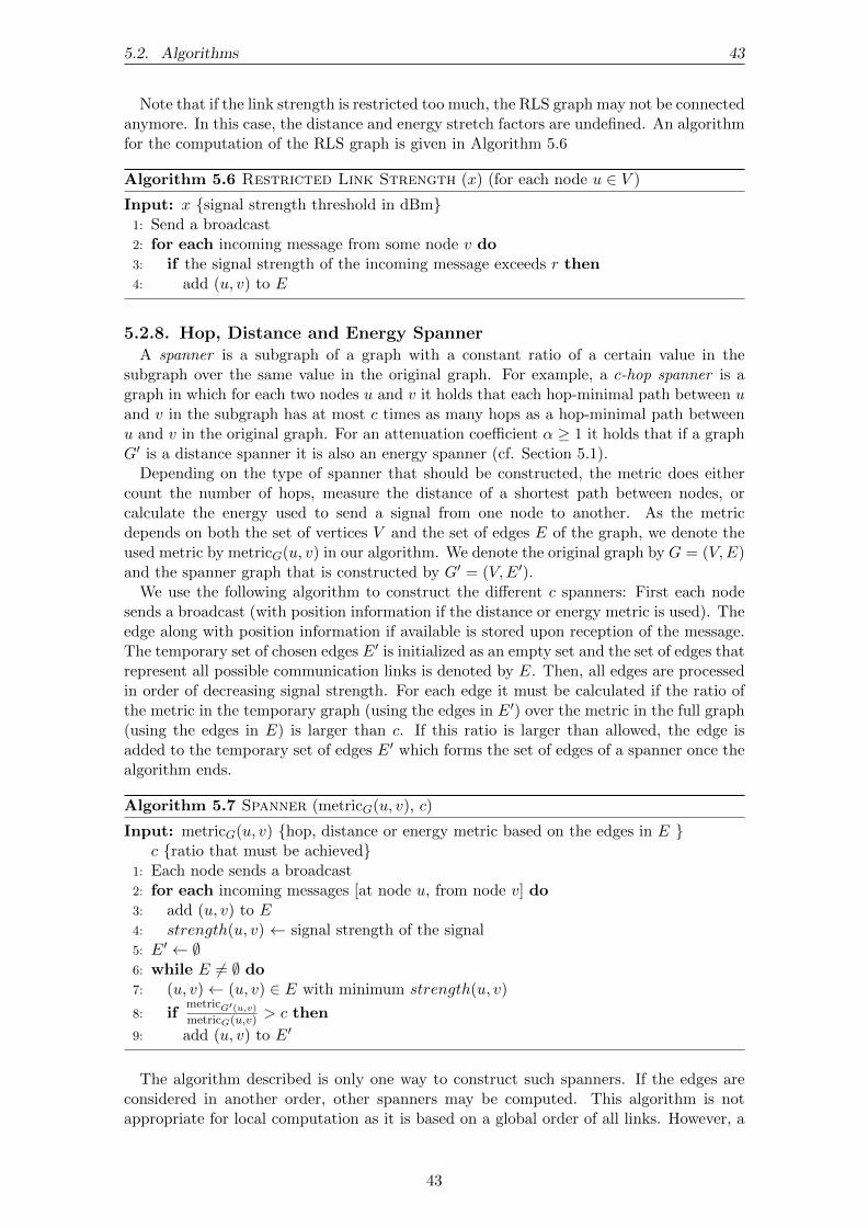
5.2. Algorithms 43
Note that if the link strength is restricted too much, the RLS graph may not be connectedanymore. In this case, the distance and energy stretch factors are undefined. An algorithmfor the computation of the RLS graph is given in Algorithm 5.6
Algorithm 5.6 Restricted Link Strength (x) (for each node u ∈ V )
Input: x {signal strength threshold in dBm}1: Send a broadcast2: for each incoming message from some node v do3: if the signal strength of the incoming message exceeds r then4: add (u, v) to E
5.2.8. Hop, Distance and Energy SpannerA spanner is a subgraph of a graph with a constant ratio of a certain value in the
subgraph over the same value in the original graph. For example, a c-hop spanner is agraph in which for each two nodes u and v it holds that each hop-minimal path between uand v in the subgraph has at most c times as many hops as a hop-minimal path betweenu and v in the original graph. For an attenuation coefficient α ≥ 1 it holds that if a graphG′ is a distance spanner it is also an energy spanner (cf. Section 5.1).
Depending on the type of spanner that should be constructed, the metric does eithercount the number of hops, measure the distance of a shortest path between nodes, orcalculate the energy used to send a signal from one node to another. As the metricdepends on both the set of vertices V and the set of edges E of the graph, we denote theused metric by metricG(u, v) in our algorithm. We denote the original graph by G = (V,E)and the spanner graph that is constructed by G′ = (V,E′).
We use the following algorithm to construct the different c spanners: First each nodesends a broadcast (with position information if the distance or energy metric is used). Theedge along with position information if available is stored upon reception of the message.The temporary set of chosen edges E′ is initialized as an empty set and the set of edges thatrepresent all possible communication links is denoted by E. Then, all edges are processedin order of decreasing signal strength. For each edge it must be calculated if the ratio ofthe metric in the temporary graph (using the edges in E′) over the metric in the full graph(using the edges in E) is larger than c. If this ratio is larger than allowed, the edge isadded to the temporary set of edges E′ which forms the set of edges of a spanner once thealgorithm ends.
Algorithm 5.7 Spanner (metricG(u, v), c)
Input: metricG(u, v) {hop, distance or energy metric based on the edges in E }c {ratio that must be achieved}
1: Each node sends a broadcast2: for each incoming messages [at node u, from node v] do3: add (u, v) to E4: strength(u, v) ← signal strength of the signal5: E′ ← ∅6: while E 6= ∅ do7: (u, v)← (u, v) ∈ E with minimum strength(u, v)
8: ifmetricG′(u,v)metricG(u,v) > c then
9: add (u, v) to E′
The algorithm described is only one way to construct such spanners. If the edges areconsidered in another order, other spanners may be computed. This algorithm is notappropriate for local computation as it is based on a global order of all links. However, a
43

44 5. Topology Control
localized computation of spanners is possible. An algorithm that constructs a spanner forfixed or variable transmission powers is described in [PR10].
Note that calculating the metric-function metricG() is trivial for the hop and distancespanner. For the energy spanner, a breadth-first search using the edges in E is sufficient.
5.2.9. Visual ComparisonIn order to gain a first impression of the topologies computed by the described topology
control algorithms, we compare the topology computed for a random network visually inthis section. Small dots visualize the position of a wireless sensor node while for eachcommunication link that is selected by the topology a black edge is drawn between thesensor nodes. We used 40 nodes on an area of 200×200 meters for this visual comparison.
0
1
2
3
4
5
6
7
89
10
11
12
13
14
15
16
17
18
19
20
21
22
23
24
25
26
27
28
29
30
31
32
33
34
35
36
37
38
39
(a) 2-hop spanner
0
1
2
3
4
5
6
7
89
10
11
12
13
14
15
16
17
18
19
20
21
22
23
24
25
26
27
28
29
30
31
32
33
34
35
36
37
38
39
(b) 3-hop spanner
0
1
2
3
4
5
6
7
89
10
11
12
13
14
15
16
17
18
19
20
21
22
23
24
25
26
27
28
29
30
31
32
33
34
35
36
37
38
39
(c) 5-hop spanner
Figure 5.1.: Visual comparison of different hop spanners.
Before comparing all considered topologies, we consider the topologies constructed fordifferent parameters c of the spanner algorithm. In Figure 5.1, the various c-hop spannersare depicted. We can see that the as the parameter c decreases more long communicationlinks are added between nodes that are relatively far away. The underlying structurewhich ensures connectivity remains mostly the same. For the distance spanners depicted
0
1
2
3
4
5
6
7
89
10
11
12
13
14
15
16
17
18
19
20
21
22
23
24
25
26
27
28
29
30
31
32
33
34
35
36
37
38
39
(a) 1.1-distance spanner
0
1
2
3
4
5
6
7
89
10
11
12
13
14
15
16
17
18
19
20
21
22
23
24
25
26
27
28
29
30
31
32
33
34
35
36
37
38
39
(b) 1.5-distance spanner
0
1
2
3
4
5
6
7
89
10
11
12
13
14
15
16
17
18
19
20
21
22
23
24
25
26
27
28
29
30
31
32
33
34
35
36
37
38
39
(c) 2.5-distance spanner
Figure 5.2.: Visual comparison of different distance spanners.
in Figure 5.2, the amount of long links that are added is lower. Only very few links in the1.1-distance spanner are as long as some of the links in the 2-hop spanner. We can also seethat the density of the network seems relatively homogeneous. The energy spanner shownin Figure 5.3 are considerably less dense. This is due to the cubically increase of energyconsumption with the communication distance. Hence, a longer detour using shorter edgesis often more energy efficient that the direct communication.
44

5.3. Simulation Setup 45
0
1
2
3
4
5
6
7
89
10
11
12
13
14
15
16
17
18
19
20
21
22
23
24
25
26
27
28
29
30
31
32
33
34
35
36
37
38
39
(a) 1.1-energy spanner
0
1
2
3
4
5
6
7
89
10
11
12
13
14
15
16
17
18
19
20
21
22
23
24
25
26
27
28
29
30
31
32
33
34
35
36
37
38
39
(b) 2-energy spanner
0
1
2
3
4
5
6
7
89
10
11
12
13
14
15
16
17
18
19
20
21
22
23
24
25
26
27
28
29
30
31
32
33
34
35
36
37
38
39
(c) 5-energy spanner
Figure 5.3.: Visual comparison of different energy spanners.
In Figure 5.4, the toplogies computed by all considered algorithms are depicted. Wecan see that all topologies reduce the density considerably by comparing them to the ALGtopology depicted in 5.4(a). Both the 1.1-distance spanner and the Yao graph are relativelydense, however, the possible communication links are distributed relatively homogeneousover the network. The EMST, XTC and the GG are rather sparse topologies. The EMSThas clearly the lowest number of edges, followed by XTC and the Gabriel graph; this is infact an inclusion relation. The 1.1-energy spanner is not in this relation, however its densityseems to be somewhere between the XTC and the Gabriel graph. The visual impression ofthe 2-hop spanner seems relatively orderdered, with some relatively long edges spanningacross large parts of the network. The RLS restricts the used communication links torelatively strong links. The distribution seems not very homogeneous over the networkbut depends on the node density within the network.
5.3. Simulation SetupIn this section, we describe the models and parameters that we used in the ns-3 simulator.
For a description of the models of a standard wireless setup, see Section 3.3.1. Throughoutthis thesis, we use ns-3 in version 3.13, which is has been released on December 23, 2011.
As there is a description of the general setup of our wireless network in Section 4.4.1, wewill only highlight the changes that apply for this chapter. In Chapter 4, a constant-raterate-control-manager has been used to achieve better comparability. In this chapter, how-ever, a more realistic behavior of our nodes is required. Therefore, the IdealWifiManager
is used for rate-control and hence varying data rates based on the SINR of the communi-cation link are used. In this chapter, we restrict the transmissions to the TCP protocolimplemented by TcpNewReno since reliable data transfer is desired. The other parts of thegeneral wireless setup in Section 4.4.1 also apply to this chapter. This includes the propaga-tion loss according to the log-distance model with parameters L0 = 46.6777, d0 = 1, α = 3and the physical layer according to YansWifiPhy::Default.
5.3.1. Parameters and ModificationsTo realize a more adequate behavior of the sending application as well as the used
protocols, some adaptions to the default protocol parameters and the protocol behavior ofns-3 had to be made:
• The TCP buffer size for sending (TcpSocket::SndBufSize) is set to the amount ofdata to be transferred. Since the OnOffApplication, which is used for generatingthe traffic, does not care about loosing data, a small TCP sending buffer may getfilled completely and data is lost. In this case, a reception of the required amount ofdata at the receiver would not be possible.
45
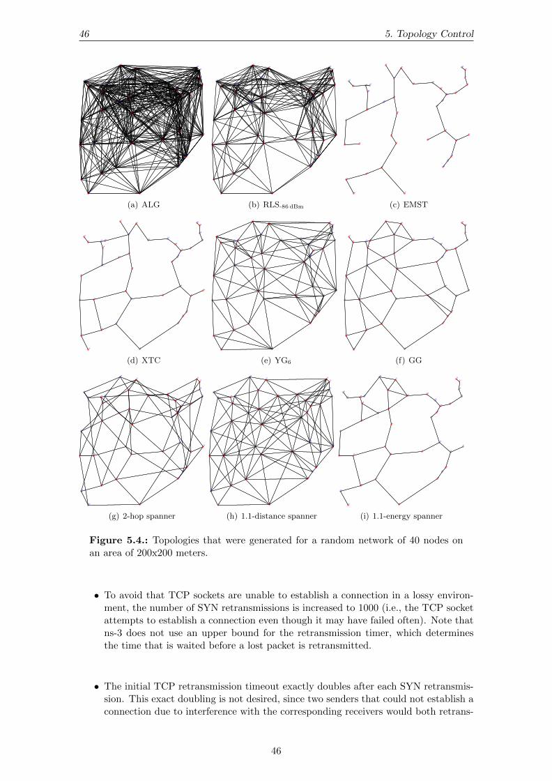
46 5. Topology Control
0
1
2
3
4
5
6
7
89
10
11
12
13
14
15
16
17
18
19
20
21
22
23
24
25
26
27
28
29
30
31
32
33
34
35
36
37
38
39
(a) ALG
0
1
2
3
4
5
6
7
89
10
11
12
13
14
15
16
17
18
19
20
21
22
23
24
25
26
27
28
29
30
31
32
33
34
35
36
37
38
39
(b) RLS-86 dBm
0
1
2
3
4
5
6
7
89
10
11
12
13
14
15
16
17
18
19
20
21
22
23
24
25
26
27
28
29
30
31
32
33
34
35
36
37
38
39
(c) EMST
0
1
2
3
4
5
6
7
89
10
11
12
13
14
15
16
17
18
19
20
21
22
23
24
25
26
27
28
29
30
31
32
33
34
35
36
37
38
39
(d) XTC
0
1
2
3
4
5
6
7
89
10
11
12
13
14
15
16
17
18
19
20
21
22
23
24
25
26
27
28
29
30
31
32
33
34
35
36
37
38
39
(e) YG6
0
1
2
3
4
5
6
7
89
10
11
12
13
14
15
16
17
18
19
20
21
22
23
24
25
26
27
28
29
30
31
32
33
34
35
36
37
38
39
(f) GG
0
1
2
3
4
5
6
7
89
10
11
12
13
14
15
16
17
18
19
20
21
22
23
24
25
26
27
28
29
30
31
32
33
34
35
36
37
38
39
(g) 2-hop spanner
0
1
2
3
4
5
6
7
89
10
11
12
13
14
15
16
17
18
19
20
21
22
23
24
25
26
27
28
29
30
31
32
33
34
35
36
37
38
39
(h) 1.1-distance spanner
0
1
2
3
4
5
6
7
89
10
11
12
13
14
15
16
17
18
19
20
21
22
23
24
25
26
27
28
29
30
31
32
33
34
35
36
37
38
39
(i) 1.1-energy spanner
Figure 5.4.: Topologies that were generated for a random network of 40 nodes onan area of 200x200 meters.
• To avoid that TCP sockets are unable to establish a connection in a lossy environ-ment, the number of SYN retransmissions is increased to 1000 (i.e., the TCP socketattempts to establish a connection even though it may have failed often). Note thatns-3 does not use an upper bound for the retransmission timer, which determinesthe time that is waited before a lost packet is retransmitted.
• The initial TCP retransmission timeout exactly doubles after each SYN retransmis-sion. This exact doubling is not desired, since two senders that could not establish aconnection due to interference with the corresponding receivers would both retrans-
46

5.3. Simulation Setup 47
mit at exactly the same time after the back-off2. Therefore the doubled retrans-mission timeout is multiplied by a uniformly distributed random value in the range[0.99, 1.01]. This is not a parameter that can be adjusted in ns-3, but a modificationto the ns-3 code. A patch can be found in Appendix A.1.
• Since we frequently use dense instances that result in transmissions with high inter-ference, packets are lost. If the Address Resolution Protocol (ARP) is not able toretrieve the address of a node, the node is flagged as dead for 100 seconds by default.This timeout (ArpCache::DeadTimeout) is decreased to 5 seconds in order to giveother transmissions a short time to finish but to also give back-off control back toTCP fast.
• Additionally, the number of retransmissions of the ARP-Request (ArpCache::Max-Retries) is slightly increased from 3 to 5, to enable a more stable ARP behaviorthroughout the simulations.
The energy detection threshold in ns-3 is set to -96 dBm by default. Thus, communica-tion links that have a signal strength of below -96 dBm are not considered strong enoughto be received. To compute topologies, we need an initial set of edges out of which thetopology control algorithm can select a subset. However, we do not simply consider allcommunication links up to the threshold of -96 dBm but give the simulator an initial phasein which each node sends 5 broadcast messages. For each node that successfully receivesat least one of the messages, a (bi-directional) communication link is added to the initialset.
This set is used by the topology control algorithms to select the subset that composesthe resulting topology, if not declared otherwise.
In the next section, we describe how ns-3 can be restricted to the communication linksselected by the topology control algorithms.
5.3.2. Routing Algorithms and NeighborhoodA channel in ns-3 distributes signals sent by any node attached to the channel to all
other nodes attached to the channel as described in Section 3.3.1. Restricting the channelwould be sufficient to ensure that packets are sent only to neighbors that are chosen usingthe topology control algorithm. One approach that would have such an effect is adding apropagation loss model that increases the path loss of packets between neighbors that arenot allowed in the topology, such that reception is impossible. Using this approach, thenetwork can communicate only over the allowed links. However, not only the desired datasignal would be restricted to the selected communication links but also interference. Sincens-3 is a packet-based network simulator, interference is received only if it is received witha packet.
This discards the propagation loss approach, since the relatively realistic modeling ofinterference is one of the reasons a network simulator is used in this thesis. Hence, thechannel-based approach to restrict communication links in ns-3 must be more complex.The interference of packets must be considered, but the packets themself must possiblybe rejected. Such an approach seems rather difficult and very likely to result in a faultysimulator behavior, due to the many low-layer adjustments that would be needed.
Neither for ns-3 nor for real-world instances it is intuitively clear where topology controlshould be mounted in the stack of protocols. So far there is no clearly favored opinion onthis problem in the literature. Two protocols are most likely to be destined for the task:The routing protocol and the protocol used in the MAC-layer.
The routing protocol is used to decide to which node a packet must be sent, if a specificdestination should be reached. For this task, it must have a list of neighbors that can be
2This does not happen very often, but it happens. This randomization is not according to RFC 2988”Computing TCP’s Retransmission Timer” [PA00].
47

48 5. Topology Control
reached and uses this list to decide which neighbor should be used to reach the destinationefficiently. For changing node positions—which are not considered in this thesis—the rout-ing protocol may also trigger the execution of the topology control algorithm dynamicallyif many links are reported to be broken.
The MAC layer controls access to the wireless medium. Hence detailed informationabout each communication link is at hand. Also, for a changing, mobile environment,the MAC layer is the first to know when the signal strength of communication links hassignificantly changed and the topology control algorithm should be executed again toprovide an updated topology.
Since we do not consider changing node positions, restricting the routing protocol toneighbors that are selected by the topology control algorithm is sufficient. Our approachto restrict the routing protocols implemented in ns-3 consists of two steps:
1. Initially provide the routing protocol with a table of allowed communication links.
2. Discard all routing protocol control messages that are received from a neighbor thatis not in the table of allowed communication links.
Since routing protocol messages are only considered from allowed communication links, itseems to the routing protocol as if messages to links that are not allowed have been lost(which is true, since they are dropped during reception at the routing layer of the receivingnode). Hence, such not-allowed communication links are not added to the routing table.Packets for a node are routed through one of the allowed communication links to reachtheir destination. The corresponding modifications to the routing algorithms are describedin Appendix A.1.
The OLSR and the DSDV routing algorithm both need some time to find the routes inthe network as they are proactive routing algorithms (cf. Section 3.4). Hence we give thealgorithms 30 seconds before the transmissions start in our experiments.
5.3.3. Test Instances and Testing EnvironmentTo ensure comparability between the different topologies, we created fixed test instances
determining the node positions and the sender-receiver pairs. We used the following pa-rameters:
Number of nodes: For our simulations, the number of nodes varies between 40 and60 nodes.
Area and node placement: On a square with base length of 50 to 550 meter, a(constant) position for each node is chosen randomly.
Number of sender-receiver pairs: Between 12 and 18 sender-receiver pairs—usingeach node only once—are chosen and saved along with the node positions in the instancefile. We use a ratio of 3 sender-receiver pairs per 10 nodes. The amount of data to betransferred between each pair is 5 MB.
For each combination of the considered parameters, 25 instances are created. The exactparameters considered are given along with the experiments.
Testing environment: The experiments were run on the same machines as those givenin Section 4.4.4. For randomization, the ns-3 seed is set to 1 for all experiments in thischapter. Each test instance is associated with its own run number. More information onthe randomization in ns-3 is given in Section 4.4.4.
To create the test instances, python has been used. Python uses the Mersenne Twisteras random number generator and is seeded by os.urandom.
Each experiment is repeated 25 times with different test instances. To ensure compara-bility between the topologies during an experiment, for each topology the same 25 inputinstances are used.
We have different representations for the results of the experiments. We mostly use
48

5.3. Simulation Setup 49
the median of our results along with error-bars which indicate the quartiles. Only inSection 5.4.2, the median of the results is sometimes given without quartile markers toenhance readability.
As some test instances (especially those that use relatively weak connection links com-bined with static routing) are not able to finish the transmissions, we used a threshold of5000 seconds after which we assume the transmissions to be failed.
5.3.4. A Note on the ThroughputWe will see in the next section that the time needed to finish transfers is surprisingly high
for the considered topologies. It is well known that the theoretical bounds of 54 Mbit/s forwireless network using IEEE 802.11a (as well as for other standards) are not achievablein practice. For packet sizes of 512 byte, about 15-20 Mbit/s are reported to be possible[DANB00]. Using the ns-3 simulator and a distance of 50 meters between two nodes (whichreduces the throughput), we achieved a maximum of 10 Mbit/s using the UDP protocoland about 8 Mbit/s using the TCP protocol. However, the results of our experiments implythat the throughput in the networks is considerably lower. For only one sender-receiverpair in the network, about 15 seconds are needed to transmit 5 MB, which equals roughly350 kB/s or 2.5 Mbit/s.
Due to the use of topologies, the number of hops on a hop-minimal path between senderand reeiver is often relatively high even for communication partners that may be withintransmission range of each other. To determine whether these hops lead to the lowerthroughput of the network, we conducted the following experiment:
For the experiment that lead to Figure 5.5, 7 nodes were placed in one row, with adistance of 50m between consecutive nodes (i.e., the x coordinate is 0 for all nodes and they coordinate is 0, 50, 100, etc.). The used topology connects each pair of adjacent nodes,which means that all edges have length 50m. In this experiment, one sender-receiver pairhad to transmit 5 MB of data over a varying number of hops. We measured the timeneeded to finish the transmission and calculated the throughput according to the timeneeded to transmit the data from the sender to the receiver.
1 2 3 4 5 6Number of hops
0
1000
2000
3000
4000
5000
6000
7000
8000
9000
Thr
ough
put
(kbi
t/s)
0
5
10
15
20
25
30
35
40
Tim
e(s
)
Figure 5.5.: Throughput vs. number of hops in a network consisting of a chain ofnodes with 50 meters between two neighboring nodes. The bars show the throughputin kbit/s, while the dashed line describes the time needed to finish the transmission.
We can see that the throughput decreases rapidly as the number of hops is increased.This is due to the fact that most nodes are in the interference range of others. In thissmall setting, only one or two nodes can send at the same time, due to the CSMA/CAmechanism that delays transmission if another node within range is transmitting.
49
50 5. Topology Control
5.4. Experiments IComparing topologies is a difficult task, since there are many different quality criteria
for topologies, as described in Section 5.1. Even worse, some of the criteria conflict withothers. Low stretch factors, for example, often imply denser topologies as more commu-nication links must be selected to achieve the low stretch factor. For other criteria, suchas throughput or interference, results are based on mathematical models which abstractfrom aspects concerning the signal transmissions and protocol behavior, hence the impacton real applications is not clear.
In this section, we use the network simulator ns-3 to compare the considered topologies.By comparing the topologies regarding the throughput that can be achieved, we are ableto study the influence of interference as well as other factors. This enables us to examinethe influence of sparse topologies on the throughput-performance and ultimately the con-nection between sparse topologies and interference minimization. We consider two mainscenarios for wireless sensor networks.
In the first scenario, which is considered in the remainder of this section, the topologycontrol algorithm computes a topology that is used by the routing algorithm to directtraffic from senders to receivers. The senders and receivers may be separated by severalhops, hence multi-hop communication may be needed. We use the IEEE 802.11a protocolwith the parameters and modifications as described in Section 5.3. In the experiments, itis studied how long it takes to transmit a uniform amount of data from the senders to thereceivers using the different topologies.
In Sections 5.4.2 to 5.4.4, we consider several parameters, such as restrictions on thelink strength, varying amounts of workload and different node densities. The throughput-performance as well as the overall energy consumption are studied for fixed as well as forvariable transmission powers in Section 5.4.5.
The second scenario uses the links of the considered topologies as input for schedulingalgorithms. We use the scheduling algorithms that have been introduced in Chapter 4 tocompare the performance of the topologies in combination with TDMA scheduling. In theliterature, scheduling of all communication links in a topology is sometimes seen as a met-ric for interference induced by the topology (cf. [WW07, page 109-112]). However, we usea slightly different approach, which is introduced in Section 5.5, since we find that schedul-ing of all communication links in the topology prefers sparse topologies excessively. Weconsider the combination of scheduling and topology control in more detail in Section 5.5along with experiments in Section 5.6.
5.4.1. Hop, Distance and Energy SpannerBeing a hop, distance or energy spanner is considered a valuable attribute for network
topologies. If a topology control algorithm computes, for example, a 2-distance spanner,it is guaranteed that the signal must travel at most twice the optimal distance if only thecommunication links of the topology are used. Unlike most other algorithms that computespanning topologies, for the spanner algorithms described in Section 5.2.8, c ≥ 1 is aparameter that the algorithm uses to construct a c spanner. This enables us to computespanner topologies for various values of c and hence to study the spanners for differentstretch factors.
The parameter c is twofold. For a parameter c that is close to 1, only few links can bediscarded. For a large c, however, a long detour, and therefore higher energy consumption,is probable. In order to decide for which parameter c good results are obtained, thefollowing experiments were conducted. In these experiments, the time needed to finish alltransmissions is measured.
We used an area of 200×200 meters is used and 60 nodes are randomly placed on thisarea for each test instance. 18 random sender-receiver pairs are associated to each instance.There is no restriction on the link strength in these experiments, but the algorithm con-siders strong communication links before weaker ones are considered. As described in
50

5.4. Experiments I 51
Section 5.3.3, for the different parameters c of the spanner algorithm the same test in-stances are used for better comparability. For hop, distance and energy spanners the timeneeded to transmit 5 MB of data between the 18 random sender-receiver pairs is measured.The main marker shows the median while the error-bars indicate the quartiles.
1.10 1.25 1.50 1.75 2.00c
0
200
400
600
800
1000
1200
1400
Tim
e(s
)
Hop-minimal RoutingShortest-Path RoutingOLSRDSDV
Figure 5.6.: Time needed to transmit all data for different c-distance spanners independence of c.
We consider the distance spanners first. As depicted in Figure 5.6, for values of cbetween 1.1 and 2, the time needed to finish all transmissions decreases as the parameterc decreases for all routing algorithms. The gain from having shorter distances and hencealso usually less hops outweighs the disadvantage of the weaker links that are added asthe distance stretch factor decreases.
We can also see that the static routing algorithms yield slightly better results for distancespanners than the build-in routing algorithms OLSR and DSDV. This is probably due tothe lower overhead of the static routing algorithm as they do not update the topologyinformation during the transmissions.
As the distance spanner yields the best results for the parameter c = 1.1, we will usethe 1.1-distance spanner in the following experiments.
Regarding hop spanners, we can see in Figure 5.7(a) that the static routing algorithms,namely the hop-minimal and the shortest-path routing, can not achieve steady resultsfor hop spanners. The hop-minimal routing algorithm does partially work for parametersbetween 4 and 6, but fails to finish the transfers for lower values of c. The shortest-pathrouting does not perform too bad, as the median of the time needed to finish the transfersfor the shortest-path routing is generally the best value. However, this is highly dependenton the instance as for most parameters more than 25 percent of the instances have notfinished the transfers within 1400 seconds.
This is due to the fact that for most instances some communication links with very lowsignal strength are selected since they span over large parts of the network. Those linksare likely to be chosen by the shortest-path and the hop-minimal routing algorithms forsome instances.
In Figure 5.7(b), the results are depicted for energy spanners with an energy stretchfactor between 1.1 and 2. For the energy spanners, the static routing algorithms performwell. Both the hop-minimal and the shortest-path routing perform best for all energystretch factors. This is due to the optimal routes as well as the lower overhead for thestatic routing algorithms.
For the OLSR routing we can see that the time needed to finish all transmissions in-creases more than for the other routing algorithms as the energy stretch factor increases.It can be observed that the OLSR routing is less performant regarding the throughput asthe topology is getting increasingly sparse. This increase is probably connected to ineffi-cient behavior of OLSR in sparse networks. The OLSR routing protocol has been designed
51

52 5. Topology Control
1.10 1.25 1.50 1.75 2.00c
0
200
400
600
800
1000
1200
1400T
ime
(s)
Hop-minimal RoutingShortest-Path RoutingOLSRDSDV
(a) c-hop spanners
1.10 1.25 1.50 1.75 2.00c
0
200
400
600
800
1000
1200
1400
Tim
e(s
)
Hop-minimal RoutingShortest-Path RoutingOLSRDSDV
(b) c-energy spanner
Figure 5.7.: Hop and energy spanner for different values of c.
for dense networks and it has been reported to have issues with sparse networks [FR09].Those issues may be connected to the multi-point relays, which do not work properly insparse networks, or to flooding of OLSR TopologyControl messages (cf. Section 3.4) insparse networks. The DSDV algorithm shows a performance similar to the static routingalgorithms but needs about 25 percent more time to finish the transmissions. The gen-eral overhead of the build-in routing algorithms in contrast to the hop-minimal and theshortest-path routing is probably again due to the higher overhead to maintain the routesand the fact that the computed routes are not necessarily optimal.
5.4.2. Restricting the Link Strength
Wireless reception hardware restricts communication to communication links that achievea received signal strength higher than a certain threshold. If the energy of a signal is be-low this threshold, the signal can not be decoded—even without interference—due to thelimited sensitivity of the receiver. In ns-3, this energy is defined by the energy detectionthreshold of -96 dBm.
However, a topology control algorithm can also restrict the link strength by selectingonly communication links that exceed a certain threshold. A simple algorithm that usessuch a threshold is the RLS algorithm described in Section 5.2.7. RLS has a similarbehavior as the spanner graphs: For a low threshold, only few edges are removed. For ahigh threshold, the throughput in the resulting network topology may suffer, as only fewlinks are available or the network may not even be connected. Therefore, a good thresholdhas to be found.
In this section, we study how the throughput of the network is affected by restricting thetopology to links whose signal strength exceed a certain threshold. For the experiments,a setup of 60 nodes on a square with 200 meter base length is used. As usual, each one of18 sender-receiver pairs had to transfer 5 MB across the network.
Before we determine a good threshold, we first study how the restriction on communi-cation links with high signal strength influences the connectivity of the network. Sincethe RLS algorithm does not necessarily compute connected topologies, this must also beconsidered for an optimal threshold. In Figure 5.8, the percentage of our instances that arenot connected if the signal strength is restricted to the according threshold is displayed.Note that for the results in the following experiments in this section, only those instancesare considered that are connected and hence the number of considered instances decreasesfor restrictions to communication links with high signal strength.
In order to determine a signal strength threshold which allows good throughput, wemeasure the time needed to finish the transmission between the 18 random sender-receiverpairs for various thresholds. We use the same setup as in the previous experiment in this
52

5.4. Experiments I 53
−96−94−92−90−88−86−84−82−80−78−76
Signal Strength (dBm)
0
10
20
30
40
50
60
70
80
90
100
Unc
onne
cted
inst
ance
s(%
) RLS
Figure 5.8.: Percentage of unconnected instances for the RLS algorithm using dif-ferent thresholds for the restriction of links.
−96−94−92−90−88−86−84−82−80−78−76
Signal Strength (dBm)
0
100
200
300
400
500
600
Tim
e(s
)
Hop-minimal RoutingShortest-Path RoutingOLSRDSDV
Figure 5.9.: Time to finish all transmissions for restricted link strength topologiesusing the four different routing algorithms. We can see that the required time islowest for a threshold of -84 dBm or -86 dBm.
section. Note that the number of instances decreases as we restrict the communicationlinks to those that exceed a high threshold according to Figure 5.8.
In Figure 5.9, we can see that if the RLS algorithm is limited to only few but verystrong links, the resulting topology achieves acceptable, although not optimal throughput-performance. The results are not optimal mainly because the stronger communicationlinks are shorter and hence more hops are needed to reach the receiver. However, we haveseen in Figure 5.8 that many instances are not connected anymore for restrictions to highersignal strength than -80 dBm.
If many links are used by the algorithm, including some with low signal strength, routingon the topology does not perform well either. For the static routing algorithms, this isdue to the fact that the routes are chosen prior to the transmission and communicationlinks with low signal strength can not be avoided. Both, OLSR and DSDV keep track ofcommunication links that appear to be broken and avoid them. Hence, those links thatresult in high losses are not used. Thus, for OLSR and DSDV, the time needed to finishthe transmissions does not increase as dramatically as for the static routing algorithms.However, the routing algorithms still select some communication links with low signalstrength and since the rate-control manager automatically decreases the data-rate forlinks with low SINR, the performance of those routes is not optimal. Overall, the OLSRrouting protocol seems to be more robust against links with low signal strengths than theDSDV routing algorithm.
We can observe that for thresholds of -86 dBm and -84 dBm, the throughput-performanceof the routing algorithms is best on the resulting topologies.
53

54 5. Topology Control
Considering the throughput-performance as well as the expected connectivity of theinstances, we come to the conclusion that the RLS topology control algorithms with athreshold of -86 dBm yields the best results. Hence, we will use the RLS algorithm withthis threshold for our experiments; the RLS algorithm using this threshold is denoted byRLS-86 dBm.
The link strength can also be restricted for other topology control algorithms. This mayresult in different outputs and influence the properties of the generated topologies. Also,by comparing the performance of the unrestricted topologies with the performance of therestricted topologies, one may be able to draw conclusions about the signal strength of thelinks that are mainly used in the topologies.
Usually the topology control algorithms can select a subset of the set of all possibleconnection links. In this experiments, however, we restrict the input of the topology controlalgorithms to the connection links whose signal strength exceeds a certain threshold. Thetopology control algorithms must compute their topology solely based of this subset oflinks.
To study the performance of the topologies, the time they need to finish the transmissionbetween the sender-receiver pairs is measured. In Figure 5.10, this time is depicted forvarious thresholds on the restriction on the input for the topology control algorithms. Forthe experiments that led to those results, we used a setup of 60 nodes, randomly placedon a square area with base length of 200 meters. Each of the 18 random sender-receiverpairs had to transmit 5 MB of data. We used 25 instances for this experiment; In thedepicted results, the main marker indicates the median of the time needed to finish thetransmissions and the error-bars show the quartiles.
For the EMST topology used in Figure 5.10(b), the OLSR routing algorithm does notperform very well. The additional time needed to finish the transmissions is primarily dueto the overhead created by the messages sent by the OLSR algorithm along this very fewedges. Additionally, as described for the energy spanners, the OLSR algorithm does notperform well for very sparse networks.
For thresholds below -84 dBm the time needed to transmit all data for the consideredinstances decreases slightly. This is propably since the topologies that required relativelylong links in the minimal spanning tree are not considered anymore, since they are notconnected anymore (cf. Figure 5.8). For all routing algorithms except the OLSR routing,the results achieved by the EMST topology is relatively constant.
The results of the XTC algorithm are depicted in Figure 5.10(c). We can see that theperformance of the topology computed by the XTC algorithm does not change very muchwhen the subset is restricted to communication links with high signal strength. SinceXTC is based on a neighborhood criterion, mostly short links are chosen and hence therestriction on links with high signal strength has only marginal impact on the performanceof the topology computed by the XTC algorithm.
The topology based on the Yao graph, whose results are depicted in Figure 5.10(d),achieves similar results as the XTC algorithm. However the throughput is slightly betterand the difference between the routing algorithms is lower. Similar to the XTC topology,the performance does only decrease slightly as relatively strong links are discarded.
The time needed to finish the transmissions for the topology based on the Gabriel graphis depicted in Figure 5.10(e). The GG topology shows similar performance as the XTCand the YG6 topologies. However the throughput-performance of the GG-based topologyis in-between the two previously mentioned topologies.
The results for the different spanner topologies, computed according to the algorithmdescribed in Section 5.2.8, are depicted in figures 5.10(f) to 5.10(h). We can see that the2-hop spanner depicted in Figure 5.10(f) yields visually similar results as the RLS graph,however, it is about 25 percent slower. For the build-in routing algorithms the performanceis best between -84 dBm and -88 dBm while the topology does not achieve stable results
54

5.4. Experiments I 55
−96−94−92−90−88−86−84−82−80−78−76
Signal Strength (dBm)
0
200
400
600
800
1000
1200
1400
Tim
e(s
)Hop-minimal RoutingShortest-Path RoutingOLSRDSDV
(a) RLS
−96−94−92−90−88−86−84−82−80−78−76
Signal Strength (dBm)
0
200
400
600
800
1000
1200
1400
Tim
e(s
)
Hop-minimal RoutingShortest-Path RoutingOLSRDSDV
(b) EMST
−96−94−92−90−88−86−84−82−80−78−76
Signal Strength (dBm)
0
200
400
600
800
1000
1200
1400
Tim
e(s
)
Hop-minimal RoutingShortest-Path RoutingOLSRDSDV
(c) XTC
−96−94−92−90−88−86−84−82−80−78−76
Signal Strength (dBm)
0
200
400
600
800
1000
1200
1400
Tim
e(s
)
Hop-minimal RoutingShortest-Path RoutingOLSRDSDV
(d) Y G6
−96−94−92−90−88−86−84−82−80−78−76
Signal Strength (dBm)
0
200
400
600
800
1000
1200
1400
Tim
e(s
)
Hop-minimal RoutingShortest-Path RoutingOLSRDSDV
(e) GG
−96−94−92−90−88−86−84−82−80−78−76
Signal Strength (dBm)
0
200
400
600
800
1000
1200
1400
Tim
e(s
)
Hop-minimal RoutingShortest-Path RoutingOLSRDSDV
(f) 2-hop spanner
−96−94−92−90−88−86−84−82−80−78−76
Signal Strength (dBm)
0
200
400
600
800
1000
1200
1400
Tim
e(s
)
Hop-minimal RoutingShortest-Path RoutingOLSRDSDV
(g) 1.1-distance spanner
−96−94−92−90−88−86−84−82−80−78−76
Signal Strength (dBm)
0
200
400
600
800
1000
1200
1400
Tim
e(s
)
Hop-minimal RoutingShortest-Path RoutingOLSRDSDV
(h) 1.1-energy spanner
Figure 5.10.: Comparing topologies for different restrictions on the set of possiblecommunication links. This set is restricted to the links whose signal strength exceedsthe considered threshold. Note that the number of instances decreases for higherthreshold values as some instances are not connected anymore (cf. Figure 5.8).
55

56 5. Topology Control
for the static routing algorithms if all links are allowed. This is again due to the long,relatively weak links that may be added and that are likely to be chosen especially fromthe hop-minimal routing algorithm. The 1.1-distance spanner achieves stable results thatare very similar to the YG6. For the 1.1-energy spanner we can see a moderate increasein the time needed to finish the transmissions for a restriction on strong communicationlinks. Since mostly short and hence energy-efficient links are used, this is not surprising.Both built-in routing protocols show a slightly worse performance than the static routing.Again, this is probably due to the overhead which is needed to keep the routes updated.
On an overall comparison of Figure 5.10, we see that the RLS-86 dBm topology, whichuses all available communication links with a signal strength higher than -86 dBm, resultsin slightly higher throughput than the YG6 and the 1.1-distance spanner. The EMSTalgorithm does not yield a good performance, especially for the OLSR routing algorithm.It generally seems as if the built-in routing algorithms create a slightly higher overhead forsparse topologies. Without restricting the link strengths, the ALG topology does not yieldacceptable results, and hence another topology should be used if relatively weak links arenecessary to ensure connectivity.
Overall we can see that for most topologies a combination with a restriction on strongerlinks is not necessary. In the ALG, if all edges are used, a restriction yields considerablybetter results. Similarly, the 2-hop spanner yields better results if combined, the differenceshowever are not as significant as for the ALG.
5.4.3. Increasing the WorkloadIn order to see how the different topologies can cope with a varying amount of traffic,
we slowly increase the number of sender-receiver pairs in the network in the experimentsconsidered in this section.
The experiments conducted in this section use 50 nodes. The nodes were randomlypositioned on squares with base lengths of 200 meters and 400 meters, respectively. Foreach number of pairs, 25 random instances are considered. The set of communicationlinks is generally not restricted. Only for the RLS-86 dBm the signal strength is set to-86 dBm and for the EMST it is set to -90 dB to enable relatively good results even forthe OLSR routing algorithm. Since the hop-minimal routing showed similar results asthe shortest-path routing and the combination of parameters is relatively high for theseexperiments, we conducted these experiments only for the shortest-path, the OLSR andthe DSDV routing. In the following experiments, we measured the time the topologiesneeded to transmit the data from the senders to the receivers.
In Figure 5.11, we can see that the time needed to finish the transmissions is similarthroughout the different routing algorithms in the 200×200 meter setting. Only the EMSTperforms worse for the OLSR routing algorithm, as the OLSR routing does not performwell on sparse topologies. The topology that performs best for almost all numbers ofsender-receiver pairs is the RLS-86 dBm topology, which uses all communication links whosesignal strengths exceed the threshold of -86 dBm. Since the link strength is restricted tosufficiently good links, this topology enables high throughput while offering various routesand hence avoiding bottlenecks. The topologies seem to be ordered roughly according tothe densities which can be seen in the visual comparison of the topologies in Figure 5.4.The best performance besides the RLS-86 dBm topology is achieved by the YG6 and the1.1-distance spanner, followed by the topologies based on the Gabriel graph, the 1.1-energyspanner and XTC.
To confirm the assumption that the throughput performance relies on the node density ofthe network, as well as to study the different topologies more intensively, we now examinesome basic properties of the considered topologies. For the average number of hops inFigure 5.12(a), the hop-minimal path from each sender to the corresponding receiver hasbeen calculated and the mean of the number of hops is stored. The average edge degree,which is shown in Figure 5.12(b), is calculated based on the links chosen by the topologies.
56

5.4. Experiments I 57
5 10 15 20 25Number of pairs
0
200
400
600
800
1000
1200
1400
Tim
e(s
)RLSEMSTXTCYG6
GGDSES
(a) Shortest-path routing
5 10 15 20 25Number of pairs
0
200
400
600
800
1000
1200
1400
Tim
e(s
)
RLSEMSTXTCYG6
GGDSES
(b) OLSR routing
5 10 15 20 25Number of pairs
0
200
400
600
800
1000
1200
1400
Tim
e(s
)
RLSEMSTXTCYG6
GGDSES
(c) DSDV routing
Figure 5.11.: Comparing topologies using an increasing number of random sender-receiver pairs that need to transmit data for the different routing algorithms. Theused area is a square of 200×200 meters.
5 10 15 20 25Number of pairs
0
2
4
6
8
10
12
14
16
Avg
.num
ber
ofho
ps
(a) Average number of hops
5 10 15 20 25Number of pairs
0
2
4
6
8
10
12
14
16
18
20
Avg
.nod
ede
gree
(b) Average node degree
Figure 5.12.: Basic properties of the topologies considered in this experiment. Fora legend, cf. Figure 5.11.
The average number of hops is not accountable for the increase in time needed to finishthe transmissions as the number of hops increases. However, by comparing Figure 5.12(a)and Figure 5.11, we can see that the time needed to finish the transmissions (regardless ofthe number of transmission pairs considered) and the average number of hops are closelyrelated. The order of the topologies are the same for both measures and even the relative
57

58 5. Topology Control
differences between the topologies are similar for the time needed to finish the transmissionsand the average number of hops.
Regarding the average node degree of the topologies, which is depicted in Figure 5.12(b),the values extracted from the topologies confirm what we have seen in the visual compari-son in Figure 5.4. The average node degree is very low and between 2 and 4 for the EMST,XTC and the 1.1-energy spanner. For the 1.1-distance spanner and the YG6, the averagenode degree is about 7 and the RLS-86 dBm has an average node degree of roughly 15.
We may note that mainly for those topologies that need more time to finish the trans-missions there is a high fluctuation in the average time to process all transmissions. Thiscan be seen for the topologies based on XTC and the 1.1-energy spanner and especiallyfor the EMST. For those topologies, only few links connect various sender-receiver pairs.Especially for the EMST, there is only one path between each sender and receiver. Forthis reason, there are probably many communication links that are used by several sender-receiver pairs. Those links are very likely responsible for several failed TCP connectionsand hence delayed transmission.
There are many properties that differ between sparse and dense topologies, e.g., theaverage node degree and the average edge length. However, the number of nodes persquare-meter gives another measure of density, which does not depend on the used topol-ogy. In our next experiments, we consider a similar setup as earlier in this section on alarger area. The number of nodes remains at 60 nodes, but they are placed on an increasedarea of 400×400 meters. Hence, the node density is 4 times lower (in nodes per square-meter) than in the previous setup. The results of these experiments are depicted in Figure5.13 and Figure 5.14. Not that the results in Figure 5.13 show only the median, an ac-cording figure that depicts the median along with the quartiles can be found in AppendixA.3.
5 10 15 20 25Number of pairs
0
200
400
600
800
1000
1200
1400
Tim
e(s
)
RLSEMSTXTCYG6
GGDSES
(a) Shortest-path routing
5 10 15 20 25Number of pairs
0
200
400
600
800
1000
1200
1400
Tim
e(s
)
RLSEMSTXTCYG6
GGDSES
(b) DSDV routing
Figure 5.13.: The time needed to finish the transmissions for the relatively sparsetopologies on an area of 400 × 400 meters. The same figures with quartile markerscan be found in Appendix A.3.
For the shortest-path routing algorithm, we can see in Figure 5.13(a) that the topolo-gies based on the 1.1-distance spanner and the Yao graph do not produce good results.Both topologies are relatively dense and hence select many communication links. Due tothe increased deployment area, the topologies are selecting communication links that aretoo weak to enable communication with a good performance. Due to interference somecommunication links may fail completely. Since those weak links can not be avoided usingthe static routing protocol, some transmissions can not be finished. The densest topol-ogy, however, is probably the RLS algorithm which still yields very good results. Thisis due to its restriction on relatively strong links. For the other topologies, namely the1.1-energy spanner, the XTC, the Gabriel graph and the EMST their performance is again
58

5.4. Experiments I 59
roughly according to the average number of hops that are used (cf. Figure 5.15(a)). Onlythe Gabriel graph is slightly worse than expected if only the average number of hops isconsidered. This is probably due to longer and hence weaker communication links (cf.Figure 5.16(b)).
The results for the built-in routing algorithm DSDV are depicted in Figure 5.13(b). Wecan see that the resulst for those topologies that have been able to finish for the shortest-path routing algorithm is mainly similar. However, due to the possibility to avoid weaklinks in this routing algorithm, the 1.1-distance spanner and the Yao Graph can yield bet-ter results. But still the results are considerably worse than for the denser setup, especiallyif the results are considered relative to those of the other topologies.
5 10 15 20 25Number of pairs
0
200
400
600
800
1000
1200
1400
Tim
e(s
)
RLSEMSTXTCYG6
GGDSES
(a) OLSR routing without quartile markers
5 10 15 20 25Number of pairs
0
200
400
600
800
1000
1200
1400
Tim
e(s
)
RLSEMSTXTCYG6
GGDSES
(b) OLSR routing with quartile markers
Figure 5.14.: The time needed to finish the transfers for the OLSR routing algorithm.This is the only routing algorithm that achieves relatively stable results for almost allconsidered topologies on an increased area of 400× 400 meters.
For the OLSR algorithm, whose results are depicted in Figure 5.14, most topologiesachieve relatively similar performance. This is since the OLSR routing algorithm is rel-atively robust against weak links. The RLS topology is slightly better than the othertopologies, which is due to its combination of relative few hops with communication linksthat are strong enough to allow sufficient throughput. As expected, the EMST topologyis worse for the OLSR algorithm. This is due to OLSRs worse performance on sparsetopologies (cf. Section 5.4.1).
5 10 15 20 25Number of pairs
2
3
4
5
6
7
8
9
10
11
12
13
14
Avg
.num
ber
ofho
ps
(a) Average number of hops
5 10 15 20 25Number of pairs
1.5
2.0
2.5
3.0
3.5
4.0
4.5
5.0
5.5
6.0
6.5
Avg
.nod
ede
gree
(b) Average node degree
Figure 5.15.: Properties of the considered topologies for the setup on the area of400× 400 meters. For a legend, cf. Figure 5.14.
59
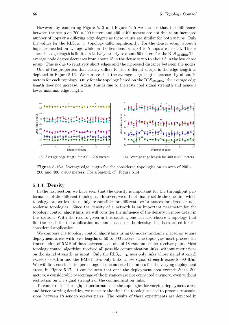
60 5. Topology Control
However, by comparing Figure 5.12 and Figure 5.15 we can see that the differencesbetween the setup on 200× 200 meters and 400× 400 meters are not due to an increasednumber of hops or a differing edge degree as these values are similar for both setups. Onlythe values for the RLS-86 dBm topology differ significantly. For the denser setup, about 2hops are needed on average while on the less dense setup 4 to 5 hops are needed. This issince the edge length is limited relatively strictly to about 50 meters for the RLS-86 dBm.Theaverage node degree decreases from about 15 in the dense setup to about 5 in the less densesetup. This is due to relatively short edges and the increased distance between the nodes.
One of the properties that clearly differs for the different setups is the edge length asdepicted in Figure 5.16. We can see that the average edge length increases by about 20meters for each topology. Only for the topology based on the RLS-86 dBm, the average edgelength does not increase. Again, this is due to the restricted signal strength and hence alower maximal edge length.
5 10 15 20 25Number of pairs
15
20
25
30
35
40
45
50
55
Avg
.edg
ele
ngth
(a) Average edge length for 200 × 200 meters
5 10 15 20 25Number of pairs
35
40
45
50
55
60
65
70
Avg
.edg
ele
ngth
(b) Average edge length for 400 × 400 meters
Figure 5.16.: Average edge length for the considered topologies on an area of 200×200 and 400× 400 meters. For a legend, cf. Figure 5.14.
5.4.4. Density
In the last section, we have seen that the density is important for the throughput per-formance of the different topologies. However, we did not finally settle the question whichtopology properties are mainly responsible for different performances for dense or not-so-dense topologies. Since the density of a network is an important parameter for thetopology control algorithms, we will consider the influence of the density in more detail inthis section. With the results given in this section, one can also choose a topology thatfits the needs for the application at hand, based on the density that is expected for theconsidered application.
We compare the topology control algorithms using 60 nodes randomly placed on squaredeployment areas with base lengths of 50 to 600 meters. The topologies must process thetransmission of 5 MB of data between each one of 18 random sender-receiver pairs. Mosttopology control algorithm received all possible communication links, without restrictionson the signal strength, as input. Only the RLS-86 dBmuses only links whose signal strengthexceeds -86 dBm and the EMST uses only links whose signal strength exceeds -90 dBm.We will first consider the percentage of unconnected instances for the varying deploymentareas, in Figure 5.17. It can be seen that once the deployment area exceeds 500 × 500meters, a considerable percentage of the instances are not connected anymore, even withoutrestriction on the signal strength of the communication links.
To compare the throughput performance of the topologies for varying deployment areasand hence varying densities, we measure the time the topologies need to process transmis-sions between 18 sender-receiver pairs. The results of these experiments are depicted in
60

5.4. Experiments I 61
50 100 150 200 250 300 350 400 450 500 550Square base length (m)
0
10
20
30
40
50
60
70
80
90
100
Unc
onne
cted
inst
ance
s(%
) ALGRLSEMSTXTCYG6
GGHSDSES
Figure 5.17.: Connectivity of the topologies for the different sizes of the deploymentarea.
Figure 5.18. Once a density is reached, for which the median of the time needed to finishthe transfers is higher than 2500 seconds, or if all instances of the topology are uncon-nected the results for this topology are no longer displayed. Note that the number of usedinstances decreases for some topologies differently than for others. For more informationcompare Figure 5.17.
From the two static routing algorithms, only the shortest-path routing is depicted. Theresults for the hop-minimal routing are similar due to the similarity of the routing algo-rithms. First some basic observations for the shortest-path routing algorithm. The topol-ogy without restrictions, ALG, does not perform well. Once a deployment area larger than100 × 100 meters is considered, the transmissions can not finish anymore. This is due toweak links, which are not avoided by the static shortest-path routing algorithm. However,for up to 100× 100 the ALG yields good results since it uses mostly one-hop connections.
For the static shortest-path routing, it can also be observed that the 2-hop spanner,the 1.1-distance spanner, the Yao Graph as well as the Gabriel graph are not able tofinish the transfers anymore for larger deployment areas in the shortest-path routing. Themajority of the transmissions can not be finished within 2500 seconds anymore for the2-hop spanner once the base length of the deployment area exceeds 200 meters, similarlyfor the 1.1-distance spanner once 300 meters are exceeded, for the Yao Graph once 350meters are exceeded and once 450 meters are exceeded for the Gabriel graph.
This is probably due to the increasing edge lengths for larger deployment areas. Asdepicted in Figure 5.19(a), for all those topologies the average edge length is about toexceed 50 meters when the topologies are no longer able to finish the transfers. However,this is probably not the exact reason why the topologies are no longer able to finish thetransmissions. As more very long links are selected to be in the topology, the averageedge length increases along with the probability that those links are chosen by the routingalgorithm. If those links are too weak, a successful transmission is hardly possible.
The topology based on RLS achieves the shortest time to finish the transmissions foralmost all densities. However, for deployment areas that exceed a base length of 450meters, the topology is only seldom able to finish the transmissions
The three remaining topologies, namely those based on the EMST, XTC and the 1.1-energy spanner, are relatively sparse and use only very few, relatively strong connectionlinks. This enables these algorithms to finish the transmissions for large deployment areaseven though the distances between the nodes are relatively high and hence almost onlyweak communications links are available. Considering only those three topologies, the1.1-energy spanner and the XTC algorithm yield the best results. The EMST needs atleast for dense networks considerably more time to finish all transmissions.
Considering denser deployment area, those three topologies need more time to finish
61
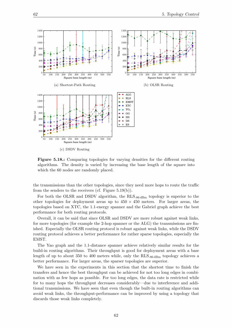
62 5. Topology Control
50 100 150 200 250 300 350 400 450 500 550Square base length (m)
0
200
400
600
800
1000
1200
1400
Tim
e(s
)
(a) Shortest-Path Routing
50 100 150 200 250 300 350 400 450 500 550Square base length (m)
0
200
400
600
800
1000
1200
1400
Tim
e(s
)
(b) OLSR Routing
50 100 150 200 250 300 350 400 450 500 550Square base length (m)
0
200
400
600
800
1000
1200
1400
Tim
e(s
)
(c) DSDV Routing
ALGRLSEMSTXTCYG6
GGHSDSES
Figure 5.18.: Comparing topologies for varying densities for the different routingalgorithms. The density is varied by increasing the base length of the square intowhich the 60 nodes are randomly placed.
the transmissions than the other topologies, since they need more hops to route the trafficfrom the senders to the receivers (cf. Figure 5.19(b)).
For both the OLSR and DSDV algorithm, the RLS-86 dBm topology is superior to theother topologies for deployment areas up to 450 × 450 meters. For larger areas, thetopologies based on XTC, the 1.1-energy spanner and the Gabriel graph achieve the bestperformance for both routing protocols.
Overall, it can be said that since OLSR and DSDV are more robust against weak links,for more topologies (for example the 2-hop spanner or the ALG) the transmissions are fin-ished. Especially the OLSR routing protocol is robust against weak links, while the DSDVrouting protocol achieves a better performance for rather sparse topologies, especially theEMST.
The Yao graph and the 1.1-distance spanner achieve relatively similar results for thebuild-in routing algorithms. Their throughput is good for deployment areas with a baselength of up to about 350 to 400 meters while, only the RLS-86 dBm topology achieves abetter performance. For larger areas, the sparser topologies are superior.
We have seen in the experiments in this section that the shortest time to finish thetransfers and hence the best throughput can be achieved for not too long edges in combi-nation with as few hops as possible. For too long edges, the data rate is restricted whilefor to many hops the throughput decreases considerably—due to interference and addi-tional transmissions. We have seen that even though the built-in routing algorithms canavoid weak links, the throughput-performance can be improved by using a topology thatdiscards those weak links completely.
62

5.4. Experiments I 63
50 100 150 200 250 300 350 400 450 500 550Square base length (m)
0
10
20
30
40
50
60
70
80
90
Avg
.edg
ele
ngth
(a) Average edge length for various densities
50 100 150 200 250 300 350 400 450 500 550Square base length (m)
0
2
4
6
8
10
12
14
16
Avg
.num
ber
ofho
ps
(b) Average number of hops for various densities
50 100 150 200 250 300 350 400 450 500 550Square base length (m)
0
5
10
15
20
25
30
35
40
45
50
55
60
Avg
.nod
ede
gree
(c) Average node degree for various densities
ALGRLSEMSTXTCYG6
GGHSDSES
Figure 5.19.: Properties of the considered topologies depending on the considereddeployment areas.
However, for networks with a very low density, long edges must probably be includedin the topology. For such applications, the sparse topologies such as those based on theXTC, EMST or the 1.1-distance spanner may be considered. Due to their restriction onrelatively short links regardless of the density of the network, the throughput for networkswith high density decreases considerably.
5.4.5. Reducing the Transmission Power
Topology control aims mainly at computing a subgraph of all possible communicationlinks that minimizes interference and energy consumption. As neither interference nor theenergy consumption are minimized if only links that are allowed for communication arelimited, so far we compared the topologies without exploiting a possible advantage. Inthe previous sections, we considered communication with a fixed, common transmissionpower. In this section, we consider scheduling with variable transmission powers for eachnode. Using fixed as well as variable transmission powers, we compare the throughputperformance as well as the energy consumption of the topologies.
In order to achieve minimal transmission powers such that each communication link thatis chosen can be used, it must be ensured that the minimal possible transmission powergrants a sufficient signal strength for each communication link. The minimal possibletransmission power for each node is computed such that the neighbor with the least recep-tion signal strength that is chosen by the topology achieves a reception signal strength of -90 dBm. If this transmission power would be higher than the default value of 16.0206 dBm3,this value is not increased. The threshold of -90 dBm has been chosen based on the results
316.0206 dBm is the default transmission power. A transmission gain of 1 dB is added by default andaccounted for in our minimal transmission powers calculations.
63

64 5. Topology Control
in Section 5.4.2, as for topologies with a signal strength of -90 dBm or above the routingalgorithms can usually finish the transmissions.
As reducing the transmission power does also reduce the range of the node’s signal, lessnodes are interfered by the signal. Hence, a faster transmission may be possible. It is alsoprobable that an overall improvement of the energy consumption can be achieved.
We will first consider the throughput performance. As before, we use the time neededto transfer the data between random sender-receiver pairs as a measure for throughputperformance. Our experiments consists of 60 nodes that are randomly placed on a squarearea of 200×200 meters. 18 random sender-receiver pairs are required to transmit 5 MBof data. In Figure 5.20 and Figure 5.21 the results of these experiments are displayed.
ALG RLS EMST XTC YG6 GG HS DS ESAlgorithm
0
500
1000
1500
2000
2500
Tim
e(s
)
(a) Fixed transmission powers
ALG RLS EMST XTC YG6 GG HS DS ESAlgorithm
0
500
1000
1500
2000
2500
Tim
e(s
)
(b) Variable transmission powers
Figure 5.20.: Time needed to finish the transmissions using the shortest-path routingalgorithm for fixed transmission powers and variable transmission powers.
ALG RLS EMST XTC YG6 GG HS DS ESAlgorithm
0
500
1000
1500
2000
2500
Tim
e(s
)
(a) Fixed transmission powers
ALG RLS EMST XTC YG6 GG HS DS ESAlgorithm
0
500
1000
1500
2000
2500
Tim
e(s
)
(b) Variable transmission powers
Figure 5.21.: A comparison of the time needed to finish the transmissions usingthe OLSR routing algorithm for fixed transmission powers and variable transmissionpowers.
For both routing algorithms, we can see that the time needed to finish the transfersincreased and hence the throughput of the algorithms decreased if variable transmissionpowers are used. Solely for the ALG algorithm this is not the case, since a reduction ofthe transmission power is usually not possible as almost every node has neighbors far awaywith a signal strength even below -90 dBm.
There are several reasons why the throughput did not increase but decrease as thetransmission power and hence the interference on other nodes is reduced. One reasonis that the signal strength that is received at the intended receiver is also lower, which
64

5.4. Experiments I 65
implies that more messages may be lost due to a lower SINR. Another reason is that theSINR that can be achieved over a connection link determines the data rate that is usedfor the transmission over this link. As the signal strength is reduced, the SINR decreasesaccordingly and hence a lower data rate may be achieved.
Another reason may be the relatively small setup. As interference propagates far anddoes also affect nodes further away, the benefits from reducing the transmission powersmay be more relevant for larger and more wide-spread networks.
So far, variable transmission powers did not show their benefits is our experiments.Considering the energy consumption, however, it is more likely that variable transmissionpowers are beneficial.
To study and compare the overall energy consumption, we need a measure thereof.As communication is consuming major parts of the energy, we assume that the energyconsumed is proportional to the number of data packets sent. As not only data packetsbut also many smaller ACK and MAC layer packets are sent, we distinguish betweendata packets and maintenance packets. Those maintenance packets are usually about 5to 40 times smaller than data packets. As data packets are 588 bytes (512 bytes payloadplus headers), we assume that one data packets needs at least 1/12000th of a second to betransmitted4. We assume that an average maintenance packet needs about 4 microsecondsto be transmitted. Hence, we calculate the energy in joule (J) that is consumed for onerun according to
consumed energy = ATPW · (# data packets
12000+
# maintenance packets
240000) (5.1)
where ATPW is the average transmission power of the nodes in the used topology in watt,”# data packets” is the number of all data packets sent during the transmission of the dataand ”# maintenance packets” is the number of maintenance packets that are sent until thetransmissions have been finished.
To calculate the overall consumed energy of the topologies during the transmissionthe average transmission power of each node is extracted and the mean over all nodesis calculated. During the simulation, each packet that is sent is categorized as data ormaintenance packet and counted accordingly. Using these values, we can compute theoverall consumed energy as defined above.
In Figure 5.22 and Figure 5.23 we examine the energy that is consumed during thetransmission of the data for the different topologies using the shortest-path and the OLSRrouting. In Figure 5.22 the energy consumption is depicted for fixed transmission pow-ers while Figure 5.23 depicts the energy consumption for variable transmission powers.For the experiments, 60 nodes are placed randomly on a square area of 200 meter baselength and each one of the 18 sender-receiver pairs must transmit 5 MB of data using thecommunication links chosen by the topology control algorithms.
In Figure 5.22, the total energy consumption of the topologies, computed according toEquation (5.1), is depicted for the shortest-path routing and OLSR routing. We can seethat the consumed energy is closely related to the time the topologies needed to finish thetransmissions. This is due to the fact that each sender tries to send its data as soon as theCSMA/CA mechanisms allows the node to send. Also, since the throughput decreases asthe number of hops increases (cf. Section 5.3.4), those networks that use a large numberof hops (and hence require many transmissions) yield a lower throughput performance.
The total energy consumed by the topologies with variable transmission powers is dis-played in Figure 5.23. The transmission power is computed for each node individuallyas the lowest possible power such that for each communication link that is included inthe topology the communication partner can be reached with a signal strength of at least-90 dBm.
41/12000th of a second would be achieved by a 54 Mbit/s connection link.
65

66 5. Topology Control
ALG RLS EMST XTC YG6 GG HS DS ESAlgorithm
0
2
4
6
8
10
12
14
Tota
lene
rgy
(J)
(a) Shortest-path routing
ALG RLS EMST XTC YG6 GG HS DS ESAlgorithm
0
2
4
6
8
10
12
14
Tota
lene
rgy
(J)
(b) OLSR routing
Figure 5.22.: Energy consumption of the topologies without reduced transmissionpower. The total energy consumption is depicted for the shortest-path and the OLSRrouting algorithms.
ALG RLS EMST XTC YG6 GG HS DS ESAlgorithm
0.0
0.5
1.0
1.5
2.0
2.5
3.0
Tota
lene
rgy
(J)
(a) Shortest-path routing
ALG RLS EMST XTC YG6 GG HS DS ESAlgorithm
0.0
0.5
1.0
1.5
2.0
2.5
3.0To
tale
nerg
y(J
)
(b) OLSR routing
Figure 5.23.: The total energy consumption of the topologies with variable trans-mission powers for the shortest-path and the OLSR routing algorithms.
Our experiments show that, once variable transmission powers are enabled, the timeneeded to finish all transmissions no longer determines the energy consumption. Topologiessuch as the EMST, the 1.1-energy spanner, the XTC algorithm and the Gabriel graph aremost efficient considering energy consumption. This is due to the fact that those algorithmstry to chose relatively short edges, which usually means that the received signal strengthis high. The selection of those strong links varies depending on the topology. It is basedon an Euclidean metric for the EMST, on an energy-metric for the 1.1-energy spanner,and on proximity-based criteria for XTC and the Gabriel graph.
The number of packets that are sent is about 5 times higher for the EMST topologythan for the RLS-86 dBm topology. However, since the transmission power grows cubically5
with the distance, the energy that is conserved due to shorter distances to the neighborsoutweighs the additional energy that is spend due to an increased number of sent packets.
The average transmission power is depicted in Figure 5.24(a), while a more detailedview on the overall energy consumption (using the DSDV algorithm) is depicted in Figure5.24(b). We observe that the order of the topologies regarding the transmission power isidentical to the one regarding the overall energy consumption. However, the transmissionpower on the left is given in dBm and thus on a logarithmic scale, in contrast to the total
5We use an attenuation coefficient of α = 3 as described in Section 5.1.
66

5.5. Topology Control and TDMA Schedules 67
energy consumption in joule. This indicates that the algorithms that are able to use avery low transmission power need to send more packets to finish the transmissions.
ALG RLS EMST XTC YG6 GG HS DS ESAlgorithm
−5
0
5
10
15
20
Avg
.TX
pow
er(d
Bm
)
(a) Average transmission power
ALG RLS EMST XTC YG6 GG HS DS ESAlgorithm
0.0
0.2
0.4
0.6
0.8
1.0
Tota
lene
rgy
(J)
(b) Energy consumption using DSDV routing
Figure 5.24.: Average transmission powers in dBm are displayed on the left whilea detailed view on the overall energy consumption for the transmissions using theDSDV routing algorithm can be seen on the right.
We can see that according to our measure the topologies that yield a good throughputperformance, such as the RLS graph or the Yao graph, can not be considered energy-efficient as they do not allow a drastically reduced transmission power. Topology controlalgorithms that allow very low transmission power feature mostly short edges and hencethey need more hops and achieve a lower throughput.
Therefore, depending on the application and the restrictions at hand, one must considerwhich topology fits best.
Note that our measure for overall energy consumption does not account for the timethe nodes are powered on or idle. We assume that the node is idle after transmission (asit does not know when the last transmission finished). We also assumed that the energyneeded for wireless communication device is solely based on the transmission power andthat the transmission power can be adjusted continuously.
5.5. Topology Control and TDMA SchedulesIn this section, we will consider joining TDMA scheduling and topology control. There
are three main reasons to do this:
1. The length of a TDMA schedule can be considered an interference measure for topolo-gies.
2. TDMA schedules yield sleep cycles that enable the nodes to conserve energy.
3. TDMA schedules are reported to yield a better performance than CSMA/CA.
We are now considering those reasons more detailed.
In the last section, the performance of traffic send between random sender-receiver pairswas the measure for the performance of the topology. As discussed in [WW07, page 109-112], the length of a transmission schedule can be a measure for interference in networks.In the literature, it is often assumed that each edge has to be scheduled once (or twice, toaccount for the bi-directionality). This may be sufficient for dense networks, however, thiswould prefer sparse network topologies immoderately, since the workload of the topologiesmay differ depending on the number of edges in the topology.
67

68 5. Topology Control
Hence, we chose to use traffic between random sender-receiver pairs to measure perfor-mance, as this yields a comparable amount of traffic that has to be transmitted through thenetwork. Since the routing algorithms in the previous experiments were mostly balancedonce sufficiently strong communication links are considered, a shortest path is chosen andevery edge on this path is added to the set of edges that needs to be scheduled. With this,method we ensure that the load is comparable for all topologies.
As discussed in Section 2.2, the wireless network device may consume up to two thirdsof the energy a wireless node requires. For CSMA/CA, the communication device must beenabled continuously to ensure availability. For TDMA schedules on the other hand, thetime slots that are assigned to the node are known and hence the wireless network devicecan be disabled in time slots the node is not participating.
TDMA schedules are reported to yield a better performance on wireless mesh networksthan CSMA/CA[BBS06a]. By joining the topologies considered earlier in this chapterwith TDMA scheduling, we can compute a schedule for the workload on a typical wirelessnetwork topology.
5.5.1. Preliminaries, Parameters and Modifications
In this section, we describe how the TDMA schedules that are based on the topologiesconsidered earlier in this chapter can be computed. Afterwards we describe the parametersthat were adapted and the modifications in the ns-3 network simulator that were necessaryfor the experiments described in the next section.
To compute the schedules, we need to select communication links of the topology thatare representative and use them as an input to the scheduling algorithms. This is done byusing random sender-receiver pairs that need to transport a specified amount of data fromthe sender to the receiver. Each communication link that is on the6 shortest path betweena sender-receiver pair is added to the set of communication links that must be scheduled.
If a communication link is selected more than once, it is also added more than once, andits payload (i.e., the amount of data that must be transmitted over this communicationlink) is calculated accordingly. An example of the selected communication links as wellas the amount of data that must be transmitted throughout the network is depicted inFigure 5.25. Communication links are drawn bolder the more sender-receiver pairs usethis link.
For these experiments, some modifications have been necessary in contrast to the ex-periments conducted in Section 5.4:
• ns-3 does not offer a MAC layer that implements TDMA schedules as mentioned inChapter 4. As an implementation of the customization of the MAC layer was notconsidered an options, some adaptions had to be made. The issues regarding thoseadaptions are discussed in Section 4.2 and the modifications that have been madeto ns-3 are described in Section 4.4.3. In short, the buffers have been minimizedand the application that is used to send data according to the TDMA schedules ismodified accordingly.
• In contrast to the previous experiments in this chapter, a constant data-rate manageris used in these experiments. The data-rate has been reduced from 24 Mbit/s (as inChapter 4) to 6 Mbit/s. This is necessary since in many topologies long links arechosen and a data rate of 24 Mbit/s can not be achieved on those links.
• As in Chapter 4, we use the number of necessary time slots for comparison. Since weuse a time slot length of 0.1 seconds, the number of time slots divided by ten equalsthe time needed to finish the transmissions.
6If between the sender and the receiver more than one shortest path exists, one may be chosen arbitrarily.
68

5.5. Topology Control and TDMA Schedules 69
0
1
2
3
4
5
6
7
8
9
1011
12
13
14
15
16
17
18
19
20
21
22
23
24
25
26
27
28
29
30
31
32
33
34
35
36
37
38
39
(a) ALG
0
1
2
3
4
5
6
7
8
9
1011
12
13
14
15
16
17
18
19
20
21
22
23
24
25
26
27
28
29
30
31
32
33
34
35
36
37
38
39
(b) RLS-86 dBm
0
1
2
3
4
5
6
7
8
9
1011
12
13
14
15
16
17
18
19
20
21
22
23
24
25
26
27
28
29
30
31
32
33
34
35
36
37
38
39
(c) EMST
0
1
2
3
4
5
6
7
8
9
1011
12
13
14
15
16
17
18
19
20
21
22
23
24
25
26
27
28
29
30
31
32
33
34
35
36
37
38
39
(d) XTC
0
1
2
3
4
5
6
7
8
9
1011
12
13
14
15
16
17
18
19
20
21
22
23
24
25
26
27
28
29
30
31
32
33
34
35
36
37
38
39
(e) YG6
0
1
2
3
4
5
6
7
8
9
1011
12
13
14
15
16
17
18
19
20
21
22
23
24
25
26
27
28
29
30
31
32
33
34
35
36
37
38
39
(f) GG
0
1
2
3
4
5
6
7
8
9
1011
12
13
14
15
16
17
18
19
20
21
22
23
24
25
26
27
28
29
30
31
32
33
34
35
36
37
38
39
(g) 3-hop spanner
0
1
2
3
4
5
6
7
8
9
1011
12
13
14
15
16
17
18
19
20
21
22
23
24
25
26
27
28
29
30
31
32
33
34
35
36
37
38
39
(h) 1.1-distance spanner
0
1
2
3
4
5
6
7
8
9
1011
12
13
14
15
16
17
18
19
20
21
22
23
24
25
26
27
28
29
30
31
32
33
34
35
36
37
38
39
(i) 1.1-energy spanner
Figure 5.25.: Shortest-path routes from the senders to the receivers. Each edge oneach route is added to the set of transmissions that must be scheduled. Bolder linksare used by more than one route and must be scheduled according to the number ofsender-receiver pairs that use this edge.
• The data that must be transmitted over the links has been reduced to 1.5 MB. Thishas been changed to adapt the number of time slots needed to finish the transmissionaccording to the reduced data-rate.
• Since all links that are chosen should be able to finish the transmission, links whosesignal strength is too low to enable successful communication should not be con-sidered. Hence, we restricted the set of available connection links (similar to theexperiments in Section 5.4.2) to those links that have a signal strength of -90 dBmor above.
• In Chapter 4 each receiver needed only one PacketSink application to receive thepackets and each sender needed only one OnOffApplication to send packets. In
69

70 5. Topology Control
this section, however, each node may need up to n instances of each application.Therefore, for both the PacketSink as well as the OnOffApplication identifiersare needed. Those identifiers are for both applications the address of the receiverconsisting of its IP address along with the used port. Each node sends all the packetit sends to a unique port at the receiver and hence the combination of address andport of the receiver is sufficient to identify the communication link. A patch thatmodifies the application accordingly is given in Appendix A.1.
• Since the SINR thresholds are decreased as the data-rate is decreased, a new SINRthreshold must be determined. Through experiments similar to those in Section 4.5.1,a threshold of 6 dBm has been determined.
Note that we do not require the time slots to be processed in such an order that ifeach slot is processed according to the schedule, a transmission would be possible fromthe sender to the receiver. This would restrict the scheduling algorithms to process thecommunication links in the order in which they are on the routes (i.e., the first link on theroute must be scheduled before the second and so on). We allow the TDMA schedulingalgorithms to schedule the communication links without considering this aspect.
Hence we can not directly compare the instances that use the CSMA/CA mechanismwith those TDMA schedules regarding the delay of the data. However, after a number ofiterations that is linear in the length of a hop-minimal shortest path from a sender to thecorresponding receiver, the throughput that can be achieved using these TDMA schedulesis comparable to the throughput achieved using the CSMA/CA mechanism.
5.6. Experiments IISince TDMA schedules allow sleep and duty cycles, they offer interesting possibilities to
conserve energy in wireless sensor networks. However, so far, especially wireless commu-nication that has high demands on throughput and transmission range does seldom utilizeTDMA schedules. In the rest of this section, we will compute TDMA schedules based onthe links chosen by the topology control algorithms. Using these schedules to simulatethe transmission of data through the network, our experiments provide insights on howwell the topologies perform for a different media access than CSMA/CA. This gives us ameasure on the practicability of the topologies in TDMA-based networks.
We will first consider the number of time slots needed to finish the transmissions, whichallows us to compare the topologies regarding the throughput that can be achieved usingTDMA scheduling. We compare the time slots needed for both fixed transmission powersas well as variable transmission powers.
Again, for variable transmission powers the transmission power is determined individ-ually for each node as the minimal transmission power such that the signal strength forany communication link selected by the topology control algorithm the signal strength isat least -90 dBm. Note that these communication links need not be selected as input forthe scheduling algorithm.
For our experiments, we used 40 nodes that are randomly placed on a square area of200×200 meters and 12 sender-receiver pairs that are used to compute the traffic thatmust be transmitted through the network. As described in the last section, for eachsender-receiver pair those links that are on a shortest-path from the sender to the receiverare used as an input for the scheduling. Communication links that are on the shortestpath between more than one sender-receiver pair are considered according to the numberof shortest paths they are on.
In Figure 5.26 the number of slots the different topologies needed to finish the trans-missions according to the TDMA schedule are depicted. The performance is shown forfixed transmission powers in Figure 5.26(a) and for variable transmission power in Fig-ure 5.26(b). The GreedyBiSINR scheduling algorithm is used for both the fixed and thevariable transmission powers.
70

5.6. Experiments II 71
ALG RLS EMST XTC YG6 GG HS DS ESAlgorithm
0
500
1000
1500
2000
2500
3000
Num
ber
ofSl
ots
(a) Fixed transmission powers
ALG RLS EMST XTC YG6 GG HS DS ESAlgorithm
0
500
1000
1500
2000
2500
3000
Num
ber
ofSl
ots
(b) Variable transmission powers
Figure 5.26.: A comparison of the number of slots the topologies needed to finishall transmissions according to the computed TDMA schedules. The GreedyBiSINRscheduling algorithm is used and the topologie uses fixed or variable transmission pow-ers. The transmission pairs are computed based on shortest paths from the randomsender-receiver pairs in the topologies.
It can be observed that the results are basically identical. As the data rate is constantlyset to 6 Mbit/s, the transmission does not suffer from a reduced SINR as it is the casefor the variable data-rate, which is used in Section 5.4. Comparing the throughput of thetopologies, we can see that the relative performance is similar to the relative performancein CSMA/CA. Only the ALG, which is actually the RLS-90 dBm algorithm since the set ofinput links is restricted to -90 dBm, achieves an even slightly better throughput than theRLS-86 dBm. This is since -86 dBm is probably not the best threshold for the RLS algorithmwhen a constant data-rate of 6 Mbit/s is used. Since the data-rate is lower, weaker linkscan achieve a better performance in this setup than in the setup used in Section 5.4.2.
Since energy conservation is one major goal in topology control as well as in wirelesssensor networks in general, we use the energy consumption assumptions described in Sec-tion 5.4.5 to calculate the energy consumption based on the transmission power and thenumber of packets that are sent. Based on the same experiment that were used in Fig-ure 5.26, the overall energy consumption for the transmission according to the TDMAschedules is depicted in Figure 5.27.
ALG RLS EMST XTC YG6 GG HS DS ESAlgorithm
0.0
0.5
1.0
1.5
2.0
Tota
lene
rgy
(J)
(a) Fixed transmission powers
ALG RLS EMST XTC YG6 GG HS DS ESAlgorithm
0.00
0.05
0.10
0.15
0.20
0.25
0.30
0.35
0.40
Tota
lene
rgy
(J)
(b) Variable transmission powers
Figure 5.27.: Energy consumption of the transmissions in the network using TDMAschedules for fixed and variable transmission powers.
71

72 5. Topology Control
For fixed transmission powers, we can observe that similar to the transmission using theCSMA/CA mechanism in Section 5.4.5, the overall energy consumption is determined bythe required number of time slots, i.e., the time needed to finish all transfers. Hence theALG (RLS-90 dBm) and the RLS topologies dominate also for the overall energy consump-tion for fixed transmission powers. For variable transmission powers, those topologies thatuse mainly very short links are best if the energy consumption is considered. Namelythose are the topologies based on the EMST, the 1.1-energy spanner and XTC. Similar tothe transmissions using the CSMA/CA algorithm, this is due to the fact that the energyincreases cubically with the distance.
We can conclude that the relative performance of the topologies for both the throughputand the overall energy consumption for instances using the TDMA scheduling are similarto the relative performance of the topologies using the CSMA/CA mechanism to managemedium access control.
However, as observed in Chapter 4, we can expect a higher throughput for TDMAschedules than for the CSMA/CA mechanism, in addition to the benefits regarding energyconsumption.
5.7. DiscussionIn this chapter, we first gave an overview on theoretical quality criteria that are often
considered in connection with topology control. However, some of those criteria, suchas the throughput or the interference, can not be easily described using mathematicalmodels. For this reason, many topology control algorithms have only been analysed usingmathematical models.
We then gave an introduction to some of these algorithms, as well as an analysis of thethroughput performance and the energy consumption of the considered algorithms usingthe network simulator ns-3.
For some of the algorithms, it has not been clear for which parameters they perform best.For the hop, distance and energy spanners, the stretch factors that yields best throughputresults have been determined. A simple but efficient approach that restricts the topology tothe connection links that achieve a signal strength above a certain threshold is considered,and a good threshold value is determined as -86 dBm in Section 5.4.2. The more classicaltopology control algorithms have also been compared regarding their robustness towardsweak links. We observed that, except for the ALG topology that allows all links, and the2-hop spanner, all topologies aim at avoiding weak links since they restrict themselves torelatively good links whenever possible.
As for different applications a different number of sender-receiver pairs may be used,we considered how the topologies perform for an increasing amount of sender-receiverpairs and hence an increasing amount of data that must be transmitted over the network.Our experiments show that for rather dense networks, most topologies can cope withan increased amount of data. The throughput for the topologies is mainly restricted bythe average number of hops that must be used in the topologies. For few hops a highthroughput can be achieved, while for many hops the throughput is considerably lower. Asimple restriction of the signal strength in the RLS graph, the YG6 and the 1.1-distancespanner yield the best results for all considered numbers of pairs.
For a denser setup, however, the situation is not so clear. Depending on the routingalgorithm, some topologies achieve only relatively unstable results. Generally, it can besaid that the sparse topologies such as those based on the XTC, the 1.1-energy spannerand the EMST, achieve the most stable results. This is due to the relatively short linksthey use.
As for only two different densities not all properties of the topologies could be considered,we studied the performance of the topologies for various different-sized deployment areas.We found that dense topologies such as the RLS graph, the YG6 or the 1.1-distance
72

5.7. Discussion 73
spanner achieve the best throughput-performance for dense networks. However, for sparsenetworks the rather dense topologies are often outperformed by sparse topologies such asthe topologies based on XTC or the 1.1-energy spanner. This implies that the throughputperformance is highly dependent on the number of hops in general. However, if the signalstrength is relatively weak for many communication links, the improvement achieved by arestriction on only those communication links with sufficient signal strength outperformsthe drawbacks of communication over many hops. Regarding the transmission power, wefind that if variable transmission powers are not enabled, the topologies that achieve thehighest throughput are most energy-efficient. This is mostly due to the fact that thosetopologies use less hops and hence conserve transmission energy.
If variable transmission powers are considered, however, topologies that use mainly shortlinks achieve a good overall energy consumption. This is since those topologies allow thenodes of the network to reduce the transmission powers dramatically. Since the energygrows cubically with the distance, this usually results in lower consumed energy even ifmore hops are needed. For variable transmission powers, the EMST, followed by the1.1-energy spanner and XTC achieve the lowest overall energy consumption.
Combining topology control with TDMA scheduling shows that the relative resultsachieved with CSMA/CA are similar to those that can be achieved when scheduling isused for medium access. Our results show that the topologies based on a restriction ofthe link strengh, followed by the YG6 and the 1.1-distance spanner, allow the highestthroughput while the topologies based on EMST, 1.1-energy spanner and XTC are mostenergy-efficient.
Regarding the question of whether sparse topologies reduce interference or not, it is hardto make definitive statements since there is no commonly accepted measure for interference.We have observed in the experiments in this chapter that dense topologies usually achievea higher throughput for dense networks, while sparse topologies are more robust towardssparse networks. This is mostly due to the number of hops that are used and not directlyrelated to interference. For sparse topologies, the number of hops required to connect twonodes is relatively high, and hence the throughput that may be achieved is considerablyreduced. The performance of multi-hop communication is, at least partially, reduced dueto interference between the nodes. Considering the transmission power however, we foundthat the transmission power can be reduced significantly for sparse topologies and hencethe interference on other nodes is reduced. However, due to the increased number of hopsthis reduction of interference does not yield a better throughput.
73


6. Conclusion
In wireless sensor networks, where energy is a valuable and scarce resource, it is importantto communicate efficiently, since inefficient communication consumes additional energy. Inthis work, we studied two techniques that can help to improve the efficiency of commu-nication in wireless sensor networks, topology control and TDMA scheduling. Topologycontrol restricts communication to a subset of the possible communication links that areassumed to achieve more efficient communication. Scheduling can be used to managemedium access by dividing the time in time slots and assigning transmissions to timeslots such that they can transmit data simultaneously. Schedule-based medium access canreduce interference and thus improve the throughput.
So far, many topology control algorithms have mainly been analyzed theoretically. Oneof the goals of this thesis was, to study the performance of those algorithms based onsimulations in a network simulator. Also, based on these simulations, the influence ofcertain properties of the topologies on the throughput and the energy efficiency is studied.We considered performance in terms of time needed to transmit the traffic generatedby random sender-receiver pairs as well as in terms of the energy consumed during thetransmission of this data. Both performance measures are studied for communication withfixed as well as with variable transmission powers.
We observed that for rather simple and static routing algorithms, topology control canhelp to considerably improve performance. The build-in routing algorithms such as OLSRand DSDV, in contrast, automatically avoid relatively weak links that appear to be brokenby themselves. This is, by itself, a form of topology control as the routing algorithm selectsa subset of the available communication links1. However, for all routing algorithms a simplerestriction to communication links that exceed a certain signal strength, which is done inthe RLS topology, improves the throughput. More refined topology control algorithmsoften select communication links in a way that significantly increases the average numberof hops on the route between two nodes. We observed that the number of hops is a veryimportant property of the topologies if we consider the throughput performance, as thetime needed to finish transmissions increases as the average number of hops does. Thisis true for communication using CSMA/CA as well as for TDMA schedules to organizemedium access.
As the density of the networks decreases, we observed that a general restriction on linksup to a certain threshold does not yield the desired results as networks are mostly notconnected anymore. For such networks, many rather dense topologies can not produce
1Note that all communication links considered have at least once been able to successfully transmit apacket.
75
76 6. Conclusion
stable results anymore as relatively weak links may be selected. For sparse networks,we found that topologies that select only few but relatively strong links achieve the moststable results. Namely those are the topologies based on EMST, the XTC or the 1.1-energyspanner.
If we consider the energy consumption for fixed transmission powers, those topologiesthat achieve the highest throughput, which coincides with the lowest average number ofhops, are most energy-efficient according to our measure2. Again, this is the RLS graph,followed by the Yao graph and a 1.1-distance spanner. For variable transmission powers,however, the topologies that consist mainly of very short links and hence allow a lowtransmission power achieve the best energy efficiency. The drawback of more transmittedpackets is more than outweighed by the reduction of transmission power.
Another motivation of this thesis in addition to a comparison of the considered topologycontrol algorithms was a further study of whether interference is minimized by sparsetopologies, as it has often been assumed. Based on the results of Chapter 5, we can saythat since the transmission power can be reduced significantly for the considered sparsetopologies, the interference on other nodes is reduced. However, we have also observedthat the throughput performance of the networks highly depends on the average number ofhops between two nodes in the network. For sparse topologies, the average number of hopsis relatively high and the throughput performance low. Hence we can conclude that eventhough the interference is reduced, this does not yield a better throughput performance.However, if we focus on energy efficiency, we observed that sparse topologies, which mostlyrely on few but relatively strong links, can minimize the energy consumption significantly.
TDMA schedules offer some benefits regarding energy consumption by enabling the useof sleep and duty cycles to the communication links and hence enabling the nodes toconserve energy in time slots, in which they are not participating. The actual performanceof TDMA schedules has been compared to the IEEE 802.11a CSMA/CA mechanism. Wefound that even though the MAC layer implemented in ns-3 is not optimized towardsTDMA schedules, the TDMA schedules yield a considerably better performance regardingthe throughput. We did also compare two slightly different interference models. Thegeneral SINR model, which accounts only for interference caused by senders and ensuresthe SINR constraint only for receivers, and the bi-directional SINR model, which accountsfor interference caused by all nodes and ensures the SINR constraint for senders as well asreceivers. In our experiments, we found that schedules based on the bi-directional SINRmodel yield slightly better results for a narrow range of SINR threshold values.
In the literature, applying TDMA schedules to topologies has mostly been consideredeither theoretically [Mos06] or as a metric for the topologies [WW07, page 108-112]. In oursimulations, we applied TDMA schedules to transmission pairs that simulated the traffic ofsender-receiver pairs. We observed that the relative performance of the topologies using theTDMA schedules is similar to the relative performance using the CSMA/CA mechanism.Thus, a restriction on links up to a certain threshold enables the highest throughput whilethe rather sparse topologies that restrict communication to very short communicationlinks, such as those based on the EMST, the XTC or the 1.1-energy spanner, resulted inthe lowest overall energy consumption.
6.1. OutlookWe observed in this thesis that topology control is vital for very simple, static routing
algorithms. Routing algorithms that have been designed for mobile wireless ad hoc net-works are already relatively robust against weak communication links. However, severaltopology control algorithms improve the throughput performance even for those routingalgorithms. The topology that simply discards all weak links achieves the best throughputperformance. Unfortunately, this topology does not necessarily yield a connected network.
2Which is based on the number of sent packets and the transmission power.
76

6.1. Outlook 77
Finding a threshold such that connectivity persists while the throughput is maximized isinteresting, however, finding such a threshold locally would be desirable. Also, integrat-ing a restriction on strong links in routing algorithms is interesting since we observed animprovement for such a combination in our experiments.
Another interesting field is interference minimization. We observed in this thesis thatinterference can be reduced by sparse topologies, however, while significantly decreas-ing the throughput. In the past years, new measures of interference have been intro-duced (most popular are the sender-centric and the receiver-centric interference models,cf. [vRWZ09]) and topologies proposed that minimize interference according to thosemeasures [MNL05, LZLD08, YDE11, LTWL11]. In [YDE11], the proposed heuristic thatreduces receiver-centric interference is compared to a minimum spanning tree regardingthe energy consumption in a simulation-based analysis. However, a further assessment ofthe implication of these new measures of interference by the means of throughput maxi-mization as well as a more thorough analysis regarding the energy consumption is anotherinteresting research direction.
77


7. Deutsche Zusammenfassung
Drahtloskommunikation ist eine der bedeutendsten Neuerungen unserer Zeit. Gerate, diedrahtlose Kommunikation ermoglichen, sind inzwischen kostengunstig und konnen viel-seitig eingesetzt werden. Sensoren, also Gerate mit denen Eigenschaften der Umwelt er-fasst und digital verarbeitet werden, konnen sich mittels Drahtloskommunikation mit an-deren Sensoren oder einer Basisstation zu einem sogenannten drahtlosen Sensornetzwerkzusammenschließen. Sensoren mit einer entsprechenden Kommunikationseinheit werdenSensorknoten genannt.
Mittels drahtloser Sensornetzwerke konnen viele alltagliche Aufgaben effizient gelost wer-den. So konnen zum Beispiel in einem Krankenhaus Patienten mit Sensoren ausgestattetwerden, die aufgezeichnete Informationen drahtlos an eine zentrale Basisstation oder direktan Arzte und Personal weiterleiten. Ein weiteres mogliches Einsatzszenario sind Krisen-gebiete, in denen die Infrastruktur weitestgehend zerstort ist. Hier konnen Sensorknotenverwendet werden um automatisch ein drahtloses Netzwerk aufzubauen und so gezieltInformationen auszutauschen.
Fur die Realisierung dieser drahtlosen Netzwerke gibt es viele von der jeweiligen An-wendung abhangige Einschrankungen, allerdings auch einige, die generell fur drahtloseSensornetzwerke gelten. Zum einen sind die Knoten nicht mit der Infrastruktur verbun-den und mussen daher eine moglichst lange Laufzeit ermoglichen und zum anderen sollensie klein und kostengunstig sein. Da kleine und kostengunstige Sensorknoten meist keineentsprechend leistungsstarke Batterie aufweisen, sollte moglichst wenig Energie verbrauchtwerden. Da drahtlose Kommunikation den Hauptteil der Energie verbraucht, muss daraufgeachtet werden, dass die Kommunikation moglichst effizient ablauft.
Die Kommunikation in drahtlosen Sensornetzwerken war in den letzten Jahren ein aktivesForschungsgebiet. Eines der interessantesten Gebiete in diesem Forschungsfeld umfasstdie Topologiekontrolle, bei der aus der Menge der moglichen Kommunikationspartner eineTeilmenge so ausgewahlt werden soll, dass Interferenz zwischen den Knoten minimiertund energieeffiziente Kommunikation ermoglicht wird. Viele der aktuell vorgeschlagenenTopologiekontroll-Algorithmen wurden in erster Linie theoretisch analysiert. Dabei wirdhaufig angenommen, dass dunne Topologien (also Topologien mit wenig Kommunikations-partnern pro Knoten) Interferenz minimieren. Ein Ziel dieser Diplomarbeit ist es, diesenZusammenhang weiter zu untersuchen. Hierzu werden wir die Leistung dieser Algorithmensowohl in Bezug auf den erzielbaren Datendurchsatz als auch in Bezug auf die Energie-effizienz mit dem Netzwerksimulator ns-3 untersuchen.Ein weiteres interessantes Forschungsgebiet ist es, den Zugriff auf das Kommunikations-medium derart zu koordinieren, dass Interferenz und Kollisionen vermieden werden. In
79

80 7. Deutsche Zusammenfassung
dieser Diplomarbeit wurden bestehende Algorithmen zur Berechnung von Ablaufplanenfur den Medienzugriff im Zeitmultiplexverfahren, sogenannte TDMA Schedules, mittelsSimulationen im Netzwerksimulator mit dem CSMA/CA Verfahren verglichen. Das CS-MA/CA Verfahren wird im IEEE 802.11a Standard fur Medienzugriff und Kollisionsver-meidung eingesetzt. Abschließend wurde die Kombination von Topologiekontrolle undTDMA Zugriffsverfahren untersucht.
Um den Datendurchsatz in Topologiekontroll-Algorithmen zu bestimmen, wird die Zeit ge-messen, die benotigt wird um Daten von einer Menge von Sender-Empfanger-Paaren durchdas Netz zu senden. Die Sender-Empfanger-Paare sind hierbei zufallig gewahlt und derdurch das Netzwerk gewahlte Weg wird durch Routenplanungs-Algorithmen festgelegt.Wir konnten in unseren Experimenten feststellen, dass fur eher dichte Netzwerke, alsoNetzwerke mit vielen Sensorknoten auf einer recht kleinen Flache, eine Einschrankung dermoglichen Kommunikationsverbindungen auf Verbindungen mit hoher Signalstarke denhochsten Durchsatz ermoglicht. Fur eher dunne Netzwerke ist dieses Verfahren zum Teilnicht mehr geeignet, da die berechnete Topologie nicht mehr unbedingt zusammenhangendist. Hier liefern eher dunne Topologien, wie die denen ein Energie-Spanner oder der XTCAlgorithmus zugrunde liegen die besten Ergebnisse.
Um den Energieverbrauch fur die Ubertragung der Daten zwischen Sender-Empfanger-Paaren des drahtlosen Sensornetzwerkes zu schatzen wurde angenommen, dass die Anzahlder gesendeten Datenpakete maßgeblich fur den gesamten Energieverbrauch ist. Unterdieser vereinfachenden Annahme zeigen unsere Experimente, dass sich der gesamte Energie-verbrauch fur feste Sendeleistungen analog zur benotigten Zeit zum Beenden der Uber-tragung verhalt. Fur variable Sendeleistungen zeigt sich ein anderes Bild. Hier dominierendie Topologien, die ausschließlich recht kurze Kanten wahlen und daher die Sendeleistungmassiv senken konnen. Dies ist vor allem die Topologie zum euklidischen minimalenSpannbaum, aber auch die Topologien, denen ein Energie-Spanner, der XTC Algorithmusoder der Gabriel Graph zugrunde liegt.Die Topologien, die einen hohen Datendurchsatz ermoglichen, konnen leider nicht alsenergieeffizient bezeichnet werden.
Fur die Untersuchung der Algorithmen zur Berechnung von TDMA Schedules, sogenannteScheduling-Algorithmen, mussten zunachst einige Anpassungen am verwendeten Netz-werksimulator ns-3 vorgenommen werden, da der Simulator Medienzugriff nach Zeitmulti-plexverfahren nicht implementiert. Durch einige Anderungen an den Simulatorparameternund dem Zeitmultiplexverfahren kann ein solches Verfahren allerdings uber den im Simu-lator implementierten Medienzugriff simuliert werden.Fur den Vergleich der Scheduling-Algorithmen mit dem CSMA/CA Verfahren wurde eineMenge an Ubertragungen zufallig auf einem Gebiet verteilt. Nun wurde unter Beruck-sichtigung eines Modells zur Einhaltung von Signal-zu-Rausch-Verhaltnissen jede Uber-tragung einem Zeitslot zugeordnet. Durch die Berucksichtigung physikalischer Gegeben-heiten nach dem Signal-zu-Rausch-Verhaltnis wird sichergestellt, dass die Ubertragungeninnerhalb eines Zeitslots alle gleichzeitig bearbeitet werden konnen. Mittels des Netzwerk-simulators wird nun ein Zeitslot nach dem anderen abgearbeitet bis die Ubertragungenalle beendet sind. Unsere Ergebnisse zeigen, dass die Ubertragungen schneller beendetsind wenn TDMA Schedules benutzt werden; TDMA Schedules also einen hoheren Daten-durchsatz erlauben als das CSMA/CA Verfahren.
Abschließend wurde die Kombination von Topologiekontroll- und Scheduling-Algorithmenuntersucht. Hierfur wurden zunachst Topologien fur das Netzwerk berechnet und an-schließend die Knotenverbindungen, die zur Ubertragung der Daten zwischen zufalligenSender-Empfanger-Paaren benutzt werden, mittels eines Scheduling-Algorithmus in Zeit-slots eingeteilt. Um den Datendurchsatz zu bestimmen wurde erneut die Zeit gemessen,die vom Netzwerksimulator benotigt wurde um alle Ubertragungen gemaß der Einteilungin Zeitslots abzuarbeiten. Hier konnte ahnlich wie zuvor festgestellt werden, dass die
80

81
Topologie, welche nur eine Einschrankung der moglichen Kommunikationsverbindungenauf Verbindungen mit hoher Signalstarke vornimmt, gute Ergebnisse erzielt. Ahnlichwie fur das CSMA/CA Verfahren orientiert sich der erwartete Energieverbrauch fur festeSendeleistungen auch fur TDMA Schedules stark an der benotigten Zeit um die Ubertra-gungen abzuschließen. Daher konnte der niedrigste erwartete Energieverbrauch fur festeSendeleistungen durch die Topologie, welche die Kommunikationsverbindungen auf signal-starke Verbindungen einschrankt, erreicht werden. Fur variable Sendeleistungen bietendie Topologien, welche eine starke Reduzierung der Sendeleistung ermoglichen, erneut diebesten Ergebnisse, allen voran die auf dem euklidischen minimalen Spannbaum basierendeTopologie.Eines der Ziele dieser Diplomarbeit war es, den Zusammenhang zwischen dunnen Topo-logien und Interferenz in drahtlosen Sensornetzwerken weiter zu untersuchen. Basierendauf den Ergebnissen in Kapitel 5 konnen wir sagen, dass der uber eine Topologie erzielbareDurchsatz nicht direkt von der Interferenz abhangt, sondern mit einigen Eigenschaftenwie der Anzahl der fur eine Ubertragung notwendigen Knoten eng verbunden ist. Durcheine Verringerung der Sendeleistungen reduzieren die betrachteten dunnen Topologien dieInterferenz auf andere Knoten, es ergibt sich aber durch die Erhohung der durchschnitt-lich notigen Knoten fur die Verbindung zweier Knoten auch ein wesentlich verringerterDatendurchsatz. Allerdings zeigen unsere Experimente klar, dass sich dunne Topologienin Bezug auf den Energieverbrauch lohnen, da in dunnen Topologien hauptsachlich kurzeund signalstarke Kommunikationsverbindungen ausgewahlt werden.
81


A. Appendix
A.1. Patches to ns-3
d i f f −r org / s r c / i n t e r n e t /model/ tcp−socket−base . cc mod/ s r c /i n t e r n e t /model/ tcp−socket−base . cc
38d39> #inc lude ”ns3/random−v a r i a b l e . h”1240 c1238 ,1239< m rto = m cnTimeout ∗ backoffCount ;−−−> UniformVariable a ;> m rto = m cnTimeout ∗ backoffCount ∗ a . GetValue
( 0 . 9 9 , 1 . 0 1 ) ;
Figure A.1.: Adding random effects to the back-off timeout of the TCP implemen-tation, as described in Section 5.3.1.
83

84 A. Appendix
d i f f −r org / s r c / a p p l i c a t i o n s /model/ onof f−a p p l i c a t i o n . cc mod/ s r c /a p p l i c a t i o n s /model/ onof f−a p p l i c a t i o n . cc
120 a121 ,126> Address> OnOffAppl icat ion : : GetPeer ( void ) const> {> NS LOG FUNCTION ( this ) ;> return m peer ;> }238 a245 ,250> void OnOffAppl icat ion : : StartFor (Time start ingTime , Time
durat ion )> {> CancelEvents ( ) ;> m startStopEvent = Simulator : : Schedule ( start ingTime , &
OnOffAppl icat ion : : StartSending , this ) ;> m startStopEvent = Simulator : : Schedule ( start ingTime+duration
, &OnOffAppl icat ion : : StopSending , this ) ;> }242 a255 ,258> i f ( ! m sendEvent . I sExpi red ( ) )> {> CancelEvents ( ) ;> }d i f f −r org / s r c / a p p l i c a t i o n s /model/ onof f−a p p l i c a t i o n . h mod/ s r c /
a p p l i c a t i o n s /model/ onof f−a p p l i c a t i o n . h109 a110 ,113> // p u b l i c i n t e r f a c e f o r s c h e d u l e c o n t r o l> void StartFor (Time start ingTime , Time durat ion ) ;>> Address GetPeer ( void ) const ;d i f f −r s r c // a p p l i c a t i o n s /model/ onof f−a p p l i c a t i o n . h sr c /
a p p l i c a t i o n s /model/ onof f−a p p l i c a t i o n . h109 a110 ,113> // p u b l i c i n t e r f a c e f o r s c h e d u l e c o n t r o l> void StartFor (Time start ingTime , Time durat ion ) ;>> Address GetPeer ( void ) const ;
Figure A.2.: Modifications to the ns-3 OnOffApplication as described in Sec-tion 4.4.3.
84

A.1. Patches to ns-3 85
d i f f −r s r c // a p p l i c a t i o n s /model/ packet−s i n k . cc s rc / a p p l i c a t i o n s /model/ packet−s i n k . cc
197 a198 ,204> Address> PacketSink : : GetLocalAddress ( void ) const> {> NS LOG FUNCTION ( this ) ;> return m loca l ;> }>d i f f −r ns−3.13/ s r c // a p p l i c a t i o n s /model/ packet−s i n k . h s rc /
a p p l i c a t i o n s /model/ packet−s i n k . h89 a90> Address GetLocalAddress ( void ) const ;
Figure A.3.: Modifications to the ns-3 PacketSink to allow an identification of theapplication as described in Section 5.5.1.
85

86 A. Appendix
d i f f −r org / s r c /aodv/model/aodv−rout ing−pro to co l . cc mod/ s r c /aodv/model/aodv−rout ing−pro to co l . cc
239 a240 ,247> std : : map<Ipv4Address , s td : : map<Ipv4Address , double> >
RoutingProtocol : : topologyMap ;>> void> RoutingProtocol : : setTopologyMap ( std : : map<Ipv4Address , s td : : map<
Ipv4Address , double> > tm)> {> RoutingProtocol : : topologyMap = tm ;> }>913 a922 ,928>> i f ( Rout ingProtoco l : : topologyMap [ sender ] [ r e c e i v e r ] != 1)> {> return ;> }> else> NS LOG DEBUG( ”AODV node ” << this << ” r e c e i v e d a AODV
packet from ” << sender << ” to ” << r e c e i v e r ) ;d i f f −r . / ns−a l l i n o n e −3.13− c l ean /ns−3.13/ s r c // aodv/model/aodv−
rout ing−p r o t o c o l . h topo−ns−3.13/ns−3.13/ sr c /aodv/model/aodv−rout ing−p r o t o c o l . h
91a92 ,93> stat ic void setTopologyMap ( std : : map<Ipv4Address , s td : : map<
Ipv4Address , double> > tm) ;>92a95 ,96>> stat ic std : : map<Ipv4Address , s td : : map<Ipv4Address , double> >
topologyMap ;
Figure A.4.: Modifications to the build-in routing algorithm DSDV. Similar changesapply for the OLSR routing algorithm. These modifications are described in Sec-tion 5.3.1.
86

A.2. Additional Figures: TDMA vs. Separate Scheduling 87
A.2. Additional Figures: TDMA vs. Separate Scheduling
GBBtheoretic
GBBUDP
GBBTCP
SEStheoretic
SESUDP
SESTCP
Algorithm
0
200
400
600
800
1000
1200
1400
1600
Num
ber
ofSl
ots
(a) SINR threshold of 8 dB
GBBtheoretic
GBBUDP
GBBTCP
SEStheoretic
SESUDP
SESTCP
Algorithm
0
200
400
600
800
1000
1200
1400
1600
Num
ber
ofSl
ots
(b) SINR threshold of 18 dB
Figure A.5.: Comparing the TDMA schedules computed by the GreedyBiBufferalgorithm to a TDMA schedule that assigns each transmission its own slot. TheSINR threshold for the scheduling algorithms is set to 8 dB on the left and 18 dB onthe right. The setup is according to Section 4.5.2
GBtheoretic
GBUDP
GBTCP
SEStheoretic
SESUDP
SESTCP
Algorithm
0
200
400
600
800
1000
1200
1400
1600
Num
ber
ofSl
ots
(a) SINR threshold of 8 dB
GBtheoretic
GBUDP
GBTCP
SEStheoretic
SESUDP
SESTCP
Algorithm
0
200
400
600
800
1000
1200
1400
1600
Num
ber
ofSl
ots
(b) SINR threshold of 18 dB
Figure A.6.: Comparing the TDMA schedules computed by the GreedyBuffer algo-rithm to a TDMA schedule that assigns each transmission its own slot. The SINRthreshold for the scheduling algorithms is set to 8 dB on the left and 18 dB on theright. The setup is according to Section 4.5.2
87

A.3. Additional Figures: Increasing the workload
5 10 15 20 25Number of pairs
0
200
400
600
800
1000
1200
1400
Tim
e(s
)
RLSEMSTXTCYG6
GGDSES
(a) Shortest-path routing
5 10 15 20 25Number of pairs
0
200
400
600
800
1000
1200
1400
Tim
e(s
)
RLSEMSTXTCYG6
GGDSES
(b) DSDV routing
Figure A.7.: The time needed to finish the transmissions for the relatively sparsetopologies on an area of 400× 400 meters.We can see that primarily for the static shortest-path routing the larger deploymentarea causes that some transmissions can not or only slowly finish for many instances.For the DSDV algorithm the transmissions can be finished for almost all instances.However, especially the 1.1-distance spanner shows a high fluctuation.
88

List of Acronyms
6LoWPAN IPv6 over low power WPAN
ACK Acknowledgement flag; used for short replies to acknowledge the receptionof a packet
ALG All Links Graph
AODV Ad-hoc On-demand Distance Vector
API Application Programming Interface
ARP Address Resolution Protocol
CCA Clear Channel Assessment
CSMA/CA Carrier Sense Multiple Access with Collision Avoidance
CSMA Carrier Sense Multiple Access
CTS Clear to Send
DCF Distributed Coordination Function
DSDV Destination-Sequenced Distance Vector
EMST Euclidean Minimal Spanning Tree
GG Gabriel Graph
GNU GNU’s Not Unix
GTNetS Georgia Tech Network Simulator
IEEE Institute of Electrical and Electronics Engineers
IPv4 Internet Protocol Version 4
IPv6 Internet Protocol Version 6
IP Internet Protocol
LTE Long Term Evolution
MAC Medium Access Control
OLSR Optimized Link State Routing
OSI Open Systems Interconnection
QoS Quality of Service
89

RFC Request for Comment; memorandum on internet standards and protocols
RLS Restricted Link Strength Graph
RNG Relative Neighborhood Graph
RTS Request to Send
SINRG Geometric Signal to Interference and Noise Ratio
SINR Signal to Interference and Noise Ratio
STL Standard Template Library
SYN Synchronize flag; used for the first packets of a connection to synchronizesequence numbers
TCP Transmission Control Protocol
TDMA Time Division Multiple Access
UAN Underwater Acoustic Network
UDP User Datagram Protocol
WAHN Wireless Ad Hoc Network
WSN Wireless Sensor Network
WiFi Wireless Fidelity (usually a IEEE 802.11 wireless network)
WiMAX Worldwide Interoperability for Microwave Access
YANS Yet Another Network Simulator
YG Yao Graph
dBm Decibel of power relative to 1mW
dB Decibel
mW Milliwatt
ns-2 Network Simulator ns-2
90

List of Figures
2.1. Unit disks and quasi unit disks . . . . . . . . . . . . . . . . . . . . . . . . . 102.2. Transmissions and the corresponding conflict graph . . . . . . . . . . . . . . 11
3.1. ns-3 software organisation . . . . . . . . . . . . . . . . . . . . . . . . . . . . 153.2. OSI layers in ns-3 . . . . . . . . . . . . . . . . . . . . . . . . . . . . . . . . . 173.3. Link layer models in ns-3 . . . . . . . . . . . . . . . . . . . . . . . . . . . . 19
4.1. Transmissions and TDMA scheduling . . . . . . . . . . . . . . . . . . . . . . 244.2. Performance of SINR / bi-directional SINR-based TDMA scheduling algo-
rithms for different SINR thresholds . . . . . . . . . . . . . . . . . . . . . . 314.3. Relative overhead of the ns-3 simulation of the TDMA schedules . . . . . . 324.4. Comparison of the SINR-based schedules with the bi-directional SINR-
based schedules . . . . . . . . . . . . . . . . . . . . . . . . . . . . . . . . . . 324.5. Performance of TDMA vs. CSMA/CA . . . . . . . . . . . . . . . . . . . . . 334.6. Comparing GreedyBiSINR TDMA schedules with a separate slot TDMA
schedule . . . . . . . . . . . . . . . . . . . . . . . . . . . . . . . . . . . . . . 344.7. Comparing GreedySINR TDMA schedules with a separate slot TDMA sched-
ule . . . . . . . . . . . . . . . . . . . . . . . . . . . . . . . . . . . . . . . . . 35
5.1. Visual comparison of different hop spanners. . . . . . . . . . . . . . . . . . . 445.2. Visual comparison of different distance spanners. . . . . . . . . . . . . . . . 445.3. Visual comparison of different energy spanners. . . . . . . . . . . . . . . . . 455.4. Visual comparison of all considered topologies . . . . . . . . . . . . . . . . . 465.5. Throughput achieved for a varying number of hops . . . . . . . . . . . . . . 495.6. Time needed to transmit all data for different c-distance spanners in depen-
dence of c. . . . . . . . . . . . . . . . . . . . . . . . . . . . . . . . . . . . . . 515.7. Hop and energy spanner for different values of c. . . . . . . . . . . . . . . . 525.8. Percentage of unconnected topologies . . . . . . . . . . . . . . . . . . . . . . 535.9. RLS for different signal strength thresholds . . . . . . . . . . . . . . . . . . 535.10. Comparing topologies for input networks with different restrictions on the
link strength . . . . . . . . . . . . . . . . . . . . . . . . . . . . . . . . . . . 555.11. Throughput-performance for an increasing number of sender-receiver pairs
on a 200m square area . . . . . . . . . . . . . . . . . . . . . . . . . . . . . . 575.13. Performance of the sparse topologies for an increasing number of sender-
receiver pairs on a 400m square area . . . . . . . . . . . . . . . . . . . . . . 585.14. The OLSR routing algorithm for an increasing workload on 400×400 meters. 595.16. Average edge length of the topologies on the 200m and 400m square area . 605.17. Connectivity of the topologies for the different sizes of the deployment area. 615.18. Comparing the topologies for different densities . . . . . . . . . . . . . . . . 625.19. Key values for the topologies on different densities . . . . . . . . . . . . . . 635.20. Time needed to finish the transmissions for fixed and variable transmission
powers using shortest-path routing . . . . . . . . . . . . . . . . . . . . . . . 64
91

5.21. Time needed to finish the transmissions for fixed and variable transmissionpowers using OLSR routing . . . . . . . . . . . . . . . . . . . . . . . . . . . 64
5.22. Energy consumption with fixed transmission powers . . . . . . . . . . . . . 665.23. Energy consumption with variable transmission powers . . . . . . . . . . . . 665.24. Transmission powers and energy consumption with variable transmission
powers . . . . . . . . . . . . . . . . . . . . . . . . . . . . . . . . . . . . . . . 675.25. Visualization of the routes of the source target pairs for the topologies . . . 695.26. Schedule of the transmission pairs based on the routes in topologies . . . . 715.27. Energy consumption of the transmissions in the network using TDMA
schedules . . . . . . . . . . . . . . . . . . . . . . . . . . . . . . . . . . . . . 71
A.1. Adding random effects to the back-off timeout of the TCP implementation 83A.2. Modifications to the ns-3 OnOffApplication . . . . . . . . . . . . . . . . . . 84A.3. Modifications to the ns-3 PacketSink . . . . . . . . . . . . . . . . . . . . . . 85A.4. Modifications to the build-in routing algorithm DSDV . . . . . . . . . . . . 86A.5. Comparing TDMA schedules with a separate slot TDMA schedule . . . . . 87A.6. Comparing TDMA schedules with a separate slot TDMA schedule . . . . . 87A.7. Performance of the sparse topologies for an increasing number of sender-
receiver pairs on a 400m square area; with quartiles . . . . . . . . . . . . . 88
92
List of Tables
5.1. Quality criteria of the considered algorithms . . . . . . . . . . . . . . . . . . 41
List of Algorithms
5.1. All Links Graph . . . . . . . . . . . . . . . . . . . . . . . . . . . . . . . . . 405.2. EMST . . . . . . . . . . . . . . . . . . . . . . . . . . . . . . . . . . . . . . . 405.3. XTC . . . . . . . . . . . . . . . . . . . . . . . . . . . . . . . . . . . . . . . . 415.4. Gabriel Graph . . . . . . . . . . . . . . . . . . . . . . . . . . . . . . . . . . 425.5. Yao Graph . . . . . . . . . . . . . . . . . . . . . . . . . . . . . . . . . . . . 425.6. Restricted Link Strength . . . . . . . . . . . . . . . . . . . . . . . . . . . . . 435.7. Hop, energy and distance spanner . . . . . . . . . . . . . . . . . . . . . . . . 43
93


Bibliography
[ASSC02] I. F. Akyildiz, W. Su, Y. Sankarasubramaniam, and E. Cayirci, Wirelesssensor networks: a survey, Computer Networks 38 (2002), 393–422.
[BBS06a] Gurashish Brar, Douglas M. Blough, and Paolo Santi, Computationally ef-ficient scheduling with the physical interference model for throughput im-provement in wireless mesh networks, Proceedings of the 12th annual inter-national conference on Mobile computing and networking (New York, NY,USA), MobiCom ’06, ACM, 2006, pp. 2–13.
[BBS06b] Gurashish Singh Brar, Douglas M. Blough, and Paolo Santi, Computation-ally efficient scheduling with the physical interference model for throughputimprovement in wireless mesh networks, Proceedings of the 12th annualinternational conference on Mobile computing and networking (New York,NY, USA), MobiCom ’06, ACM, 2006, pp. 2–13.
[BLRS03] Douglas M. Blough, Mauro Leoncini, Giovanni Resta, and Paolo Santi, Thek-neigh protocol for symmetric topology control in ad hoc networks, Proceed-ings of the 4th ACM international symposium on Mobile ad hoc networkingand computing (New York, NY, USA), MobiHoc ’03, ACM, 2003, pp. 141–152.
[Buc08] Kevin Buchin, Minimizing the maximum interference is hard, arX-iv/0802.2134 (2008).
[BvRWZ04] Martin Burkhart, Pascal von Rickenbach, Roger Wattenhofer, and AaronZollinger, Does topology control reduce interference?, Proceedings of the 5ndACM International Symposium on Mobile Ad Hoc Networking and Com-puting, MobiHoc ’04, ACM, 2004, pp. 9–19.
[CJ03] T. Clausen and P. Jacquet, Optimized link state routing protocol (OLSR),RFC 3626 (Proposed Standard), 2003.
[CLRS09] Thomas H. Cormen, Charles E. Leiserson, Ronald L. Rivest, and CliffordStein, Introduction to algorithms, 3 ed., The MIT Press, 2009.
[DANB00] A. Doufexi, S. Armour, A. Nix, and D. Bull, A comparison of HIPERLAN/2and IEEE 802.11a physical and MAC layers, Symposium on Communica-tions and Vehicular Technology, SCVT ’00, 2000, pp. 14–20.
[EE04] Tamer A. ElBatt and Anthony Ephremides, Joint scheduling and powercontrol for wireless ad hoc networks, IEEE Transactions on Wireless Com-munications 3 (2004), no. 1, 74–85.
[Erg04] Sinem C. Ergen, ZigBee/IEEE 802.15.4 Summary, Tech. report, EECSBerkeley, September 2004.
95

[FR09] Yasir Faheem and Jean Louis Rougier, Loop avoidance for fish-eye OLSR insparse wireless mesh networks, Proceedings of the 6th international confer-ence on Wireless On-Demand Network Systems and Services (Piscataway,NJ, USA), WONS ’09, IEEE Press, 2009, pp. 215–218.
[Gar07] Vijay Garg, Wireless communications and networking, 1st ed., MorganKaufmann Publishers Inc., San Francisco, CA, USA, 2007.
[GGH+01] Jie Gao, Leonidas J. Guibas, John Hershberger, Li Zhang, and An Zhu,Geometric spanner for routing in mobile networks, Proceedings of the 2ndACM International Symposium on Mobile Ad Hoc Networking and Com-puting (New York, NY, USA), MobiHoc ’01, ACM, 2001, pp. 45–55.
[GH01] Jimmi Gronkvist and Anders Hansson, Comparison between graph-based andinterference-based STDMA scheduling, Proceedings of the 2nd ACM inter-national symposium on Mobile ad hoc networking and computing (NewYork, NY, USA), MobiHoc ’01, ACM, 2001, pp. 255–258.
[GOW07] Olga Goussevskaia, Yvonne Anne Oswald, and Rogert Wattenhofer, Com-plexity in geometric SINR, Proceedings of the 8th ACM international sym-posium on Mobile ad hoc networking and computing, MobiHoc ’07, ACM,2007, pp. 100–109.
[gtn08] Georgia tech network simulator GTNetS, Online: http://www.ece.gatech.edu/research/labs/MANIACS/GTNetS/, 2008.
[GWHW09] Olga Goussevskaia, Roger Wattenhofer, Magnus M. Halldorsson, and EmoWelzl, Capacity of arbitrary wireless networks, INFOCOM, 2009, pp. 1872–1880.
[HLR08] T. R. Henderson, M. Lacage, and G. F. Riley, Network simulations with thens-3 simulator, ACM SIGCOMM’08, ACM, August 2008, p. 527.
[HM11] Magnus M. Halldorsson and Pradipta Mitra, Nearly optimal bounds for dis-tributed wireless scheduling in the SINR model, ICALP (2), 2011, pp. 625–636.
[IEE07] IEEE Std 802.11-2007, IEEE standard for information technology-telecommunications and information exchange between systems-local andmetropolitan area networks-specific requirements - part 11: Wireless lanmedium access control (MAC) and physical layer (PHY) specifications,IEEE Std 802.11-2007 (Revision of IEEE Std 802.11-1999) (2007), C1–1184.
[Kes11] Thomas Kesselheim, A constant-factor approximation for wireless capacitymaximization with power control in the SINR model, Proceedings of the22nd Annual ACM-SIAM Symposium on Discrete Algorithms, SODA ’11,SIAM, 2011, pp. 1549–1559.
[KPX07] Iyad A. Kanj, Ljubomir Perkovic, and Ge Xia, An optimal localized approx-imation scheme for euclidean MST, 17th Fall Workshop on Computationaland Combinatorial Geometry, FWCG ’07, 2007.
[KV10] Thomas Kesselheim and Berthold Vocking, Distributed contention resolu-tion in wireless networks, Proceedings of the 24th international conferenceon Distributed computing (Berlin, Heidelberg), DISC ’10, Springer-Verlag,2010, pp. 163–178.
96

[LH06] Mathieu Lacage and Thomas R. Henderson, Yet another network simulator,Proceeding from the 2006 workshop on ns-2: the IP network simulator (NewYork, NY, USA), WNS2 ’06, ACM, 2006.
[LHS05] Ning Li, Jennifer C. Hou, and Lui Sha, Design and analysis of an mst-basedtopology control algorithm, IEEE Transactions on Wireless Communications4 (2005), no. 3, 1195–1206.
[LTWL11] Tiancheng Lou, Haisheng Tan, Yuexuan Wang, and Francis C. M. Lau,Minimizing average interference through topology control, Proceedings of the7th International Symposium on Algorithms for Sensor Systems, WirelessAd Hoc Networks and Autonomous Mobile Entities, ALGOSENSORS ’11,2011, pp. 115–129.
[LZLD08] Yongzhen Liu, Xinming Zhang, Qiong Liu, and Shifang Dai, A hybrid in-terference model-based topology control algorithm, Proceedings of the 4thInternational Conference on Networked Computing and Advanced Informa-tion Management - Volume 01 (Washington, DC, USA), NCM ’08, IEEEComputer Society, 2008, pp. 42–46.
[MKHC07] G. Montenegro, N. Kushalnagar, J. Hui, and D. Culler, Transmission ofIPv6 packets over IEEE 802.15.4 networks, RFC 4944 (Proposed Standard),September 2007.
[MNL05] Kousha Moaveni-Nejad and Xiang-Yang Li, Low-interference topology con-trol for wireless ad hoc networks, ACM Wireless Networks, IEEE Press,2005.
[Mos06] Thomas Moscibroda, Topology control meets SINR: The scheduling com-plexity of arbitrary topologies, Proceedings of the 7nd ACM InternationalSymposium on Mobile Ad Hoc Networking and Computing, MobiHoc ’06,ACM, 2006, pp. 310–321.
[MWW06] Thomas Moscibroda, Roger Wattenhofer, and Yves Weber, Protocol designbeyond graph-based models, 5th Workshop on Hot Topics in Networks, Hot-Nets ’06, November 2006.
[NCc+11] Hemanth Narra, Yufei Cheng, Egemen K. Cetinkaya, Justin P. Rohrer,and James P. G. Sterbenz, Destination-sequenced distance vector (DSDV)routing protocol implementation in ns-3, Proceedings of the 4th Interna-tional ICST Conference on Simulation Tools and Techniques, SIMUTools’11, ICST, 2011, pp. 439–446.
[NKSK02] Swetha Narayanaswamy, Vikas Kawadia, R. S. Sreenivas, and P. R. Kumar,Power control in ad-hoc networks: Theory, architecture, algorithm and im-plementation of the COMPOW protocol, in European Wireless Conference,2002, pp. 156–162.
[ns211] Network simulator ns-2, Online: http://nsnam.isi.edu/nsnam/, Nov2011.
[ns311a] Network simulator ns-3, Online, http://www.nsnam.org, Dec 2011.
[ns311b] ns-3.13 manual, Online, http://www.nsnam.org/docs/release/3.13/
manual/singlehtml/index.html, Dec 2011.
97

[PA00] V. Paxson and M. Allman, Computing TCP’s retransmission timer, RFC2988 (Proposed Standard), November 2000.
[PBRD03] C. Perkins, E. Belding-Royer, and S. Das, Ad hoc On-Demand DistanceVector (AODV) Routing, RFC 3561 (Proposed Standard), 2003.
[PH09] Guangyu Pei and Tom Henderson, Validation of ns-3 802.11b phy model,Online: http://www.nsnam.org/~pei/80211b.pdf, 2009.
[PH10] Guangyu Pei and Thomas Henderson, Validation of OFDM error rate modelin ns-3, Online: http://www.nsnam.org/~pei/80211ofdm.pdf, 2010.
[PMSH10] Stylianos Papanastasiou, Jens Mittag, Erik G. Strom, and Hannes Harten-stein, Bridging the gap between physical layer emulation and network simu-lation, WCNC ’10, 2010, pp. 1–6.
[PR10] David Peleg and Liam Roditty, Localized spanner construction for ad hocnetworks with variable transmission range, ACM Trans. Sen. Netw. 7 (2010),no. 3, 25:1–25:14.
[PSB12] Bhawani Sankar Panda, D. Pushparaj Shetty, and Bijaya Kishor Bhatta,Strong minimum energy minimum interference topology in wireless sensornetworks, ICDCIT, 2012, pp. 177–187.
[San05] Paolo Santi, Topology control in wireless ad hoc and sensor networks, Wiley,2005.
[SKS06] Changsu Suh, Young-Bae Ko, and Dong-Min Son, An energy efficientcross-layer MAC protocol for wireless sensor networks, Proceedings of the2006 international conference on Advanced Web and Network Technologies,and Applications (Berlin, Heidelberg), APWeb ’06, Springer-Verlag, 2006,pp. 410–419.
[SWL04] Wen-Zhan Song, Yu Wang, and Xiang-Yang Li, Localized algorithms forenergy efficient topology in wireless ad hoc networks, Proceedings of the5nd ACM International Symposium on Mobile Ad Hoc Networking andComputing, MobiHoc ’04, ACM, 2004, pp. 98–108.
[vDL03] Tijs van Dam and Koen Langendoen, An adaptive energy-efficient MACprotocol for wireless sensor networks, Proceedings of the 1st internationalconference on Embedded networked sensor systems (New York, NY, USA),SenSys ’03, ACM, 2003, pp. 171–180.
[VKW09] Markus Voelker, Bastian Katz, and Dorothea Wagner, On the complexity ofscheduling with power control in geometric SINR, Technical Report 2009-15(2009).
[vRWZ09] Pascal von Rickenbach, Roger Wattenhofer, and Aaron Zollinger, Algo-rithmic models of interference in wireless ad hoc and sensor networks,IEEE/ACM Trans. Netw. 17 (2009), no. 1, 172–185.
[WGG10] Klaus Wehrle, Mesut Gunes, and James Gross (eds.), Modeling and toolsfor network simulation, Springer, 2010.
[WLBmW01] Roger Wattenhofer, Li Li, Paramvir Bahl, and Yi min Wang, Distributedtopology control for power efficient operation in multihop wireless ad hocnetworks, 2001, pp. 1388–1397.
98

[WW07] Dorothea Wagner and Roger Wattenhofer (eds.), Algorithms for sensor andad hoc networks, Lecture Notes in Computer Science, vol. 4621, Springer,2007.
[WZ03] Roger Wattenhofer and Aaron Zollinger, XTC: A practical topology controlalgorithm for ad-hoc networks, In 4th International Workshop on Algorithmsfor Wireless, Mobile, Ad Hoc and Sensor Networks, WMAN ’03, 2003.
[Yao82] Andrew Chi-Chih Yao, On constructing minimum spanning trees in k-dimensional spaces and related problems, SIAM J. Comput. 11 (1982), no. 4,721–736.
[YDE11] Onur Yilmaz, Orhan Dagdeviren, and Kayhan Erciyes, Interference-awaredynamic algorithms for energy-efficient topology control in wireless ad hocand sensor networks, Comput. J. 54 (2011), no. 8, 1398–1411.
[YMG08] Jennifer Yick, Biswanath Mukherjee, and Dipak Ghosal, Wireless sensornetwork survey, Computer Networks 52 (2008), no. 12, 2292–2330.
99