Analysis of Subsurface Scattering

under Generic Illumination

Y. Mukaigawa K. Suzuki Y. YagiOsaka University, Japan

ICPR2008

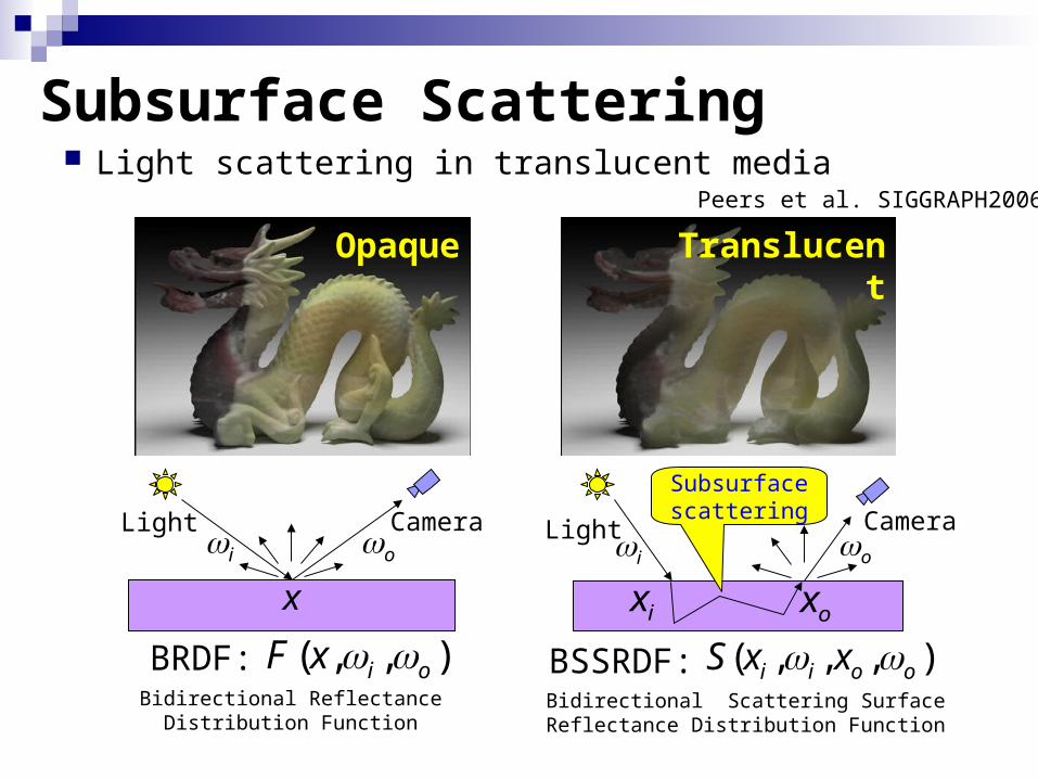
Subsurface Scattering Light scattering in translucent media

Opaque

Translucent

Light Camerai o

x

Peers et al. SIGGRAPH2006

BRDF: ),,( oixF

Light Camerai o

oxix

Subsurface scattering

BSSRDF: ),,,( ooii xxS Bidirectional Reflectance

Distribution FunctionBidirectional Scattering SurfaceReflectance Distribution Function

Translucent objects Typical translucent object

marble, milk, and skin Actually, many objects in our living environment are

also translucent.

fruit

vegetablemilk

marblesoap

candleskin

plastic

cloth

paper

eggOne of the reasons that many photometric analyzing

methods do not work well in our living environment is

they cannot treat the subsurface scattering.

Related work BSSRDF measurement using special lighting devices

Projector[Tariq et al. VMV2006]

Fiber optic spectrometer[Weirich et al. SIGGRAPH2006 ]

Laser beam[Goesele et al. SIGGRAPH2004]

Projector[Peers et al. SIGGRAPH2006]

Measurement under strictly controlled illumination

Our goal Analysis of subsurface scattering under generic illumination

Inputs: single image, 3-D shape, illuminationOutputs: reflectance properties

Inverse rendering of translucent object

3-D shape

illumination

reflectanceproperties image

rendering

inverse rendering

Known

Unknown

Dipole Model for BSSRDF Decomposition of the BSSRDF into

Fresnel functions: Ft(, )

Diffuse subsurface reflectance: R(d)

R(d) is the function of the distance d between xi and xo. Including two inherent parameters of the material

scattering coefficient: s absorption coefficient: ai

odxi xo

),( )( ),( ,, ootiit FdRF ),,,( ooii xxS

(Jensen et al. SIGGRAPH2001)

Example of R(d)

Skin（ σs=0.74,σa=0.032 ）

Apple（ σs=2.29,σa=0.003 ）0.1

0.01

0.001

0.0001

2 4 6 8 d [mm]

R(d)

Inputs:

　　　 1. Estimating R(d) for several distances d.

　　　 2. Fitting of the dipole model.

Outputs: two parameters scattering coefficient s.

absorption coefficient a.

Flow of the proposed method

Single image 3-D shape Illumination Camera parameters

+

R(d)

d

estimated R(d)

dipole model fitting

Additional information

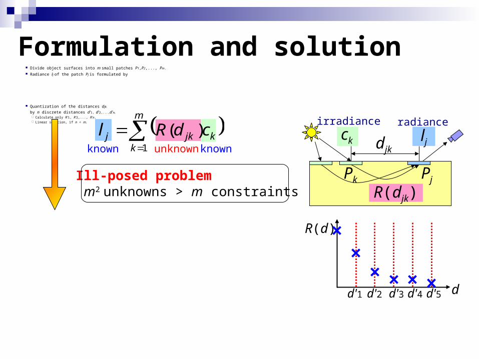
Formulation and solution Divide object surfaces into m small patches P1,P2,..., Pm.

Radiance lj of the patch Pj is formulated by

Quantization of the distances djk.

by n discrete distances d'1, d'2,...,d'n. Calculate only R'1, R'2,..., R'n. Linear solution, if n < m.

R(d)

dd'1 d'2 d'3 d'4 d'5

irradiance radiance

Pk Pj

R(djk)

ck ljdjk

m

kkjkj cdRl

1

)(unknownknownknown

Ill-posed problem m2 unknowns > m constraints

Model fitting Dipole model fitting to the estimated R'i Estimation of

scattering coefficient s absorption coefficient a

Discrete estimation R'1, ..., R'n for the quantized distances d'1, ..., d'n

Continuous estimation R(d) for every distance d

n

iii dRR

as 1

2

,)(minarg

R(d)

dd'1 d'2 d'3 d'4 d'5

R'iR(d)

Simulated scene Evaluate how the quantization of the distance affects the

accuracy of the estimated parameters.

Parameter estimation finding the best parameter set

that minimizes the error

Illumination

s=2.19a=0.002=1.3

Rendered image

parameters

s a d (mm)

Min 0.01 0.000 0.05

Max 3.00 0.010 0.50

Step 0.01 0.001 0.05

http://www.debevec.org/Probes/

Range and step of the parameters.

Results of parameter estimation

sampling

Quantization (mm) s a PSNR (dB)

0.05 2.14 0.000 26.5

0.10 2.20 0.007 42.1

0.15 2.19 0.004 30.6

0.20 2.19 0.009 33.5

0.25 2.19 0.005 28.7

0.30 2.32 0.009 29.8

0.35 2.34 0.009 47.9

0.40 2.22 0.009 25.8

0.45 2.18 0.009 20.4

0.50 2.40 0.009 23.4

Ground truth

2.19 0.002

Estimated parameters and the PSNRs

large

small

inaccurate

unstable

0

10

20

30

40

50

0.00 0.10 0.20 0.30 0.40 0.50

quantization (mm)

PSNR(dB)

best

best

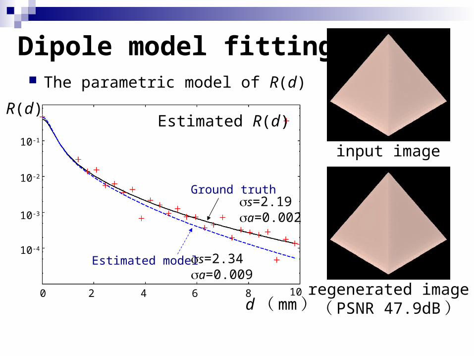
Dipole model fitting The parametric model of R(d)

input image

regenerated image（ PSNR 47.9dB ）

Estimated R(d)

d （ mm ）

R(d)

10-1

10-2

10-3

10-4

Ground truth

Estimated model

0 2 4 6 8 10

s=2.19a=0.002

s=2.34a=0.009

Real scene Evaluate the stability 3 materials:

Polypropylene (PP) Polyethylene (PE) Polyoxymethylene (POM)

2 shapes: Cube Pyramid (with base)

2 illuminations: Left and right directions.

In total, 12 images (3x2x2)

Environment for image capture

CameraCamera

Light sourceLight sourceTarget objectTarget object

Target objects

PP PE POM

Input images (3 materials x 2 shapes x 2 illuminations)

LeftRight LeftRight

Cube Pyramid

PP

PE

PO

M

Estimated parametersa

s0 1 2 3

0002

0004

0006

0008

0010

PP

PE

POM

PP POMPE

Parameters for each material Similar parameters for each

material except for some outliers. s of the cube under right

illumination is always outlier.

Averaged parameters R(d) for each material

Rendered images using estimated parametersd [mm]

R(d)10-1

10-2

10-3

10-4

0 2 4 6 8 10

PPPOM

PE

R(d)

The first step of the inverse renderingfor translucent objects.

Conclusion A new method to analyze subsurface scattering from

a single image taken under generic illumination Linear solution by quantizing the distance between patches. Parameter estimation by fitting dipole model.

Future works improvement of stability and accuracy