analysis of systems containing nonlinear and uncertain

Analysis of systems containing nonlinear and uncertain componentsby using Integral Quadratic Constraints

Tamas Peni

MTA-SZTAKI

October 2, 2012

Tamas Peni (MTA-SZTAKI) Seminar October 2, 2012 1 / 42

Contents

1 Preliminary

2 Signal spaces and operatorsSignal spacesOperatorsAdjoint operators and quadratic forms

3 Methods for analyzing the stability of feedback interconnectionsElementary system propertiesIntegral Quadratic Constraints

4 System analysis by using IQCsStability and performance specificationsLFT representationThe IQC-based analysis procedureThe Kalman-Yakubovic-Popov Lemma

5 List of IQCs

6 Beyond the analysis

7 Beyond the IQCs


Preliminary


LMIs

A Linear Matrix Inequality (LMI) is an expression of the form

F (x) = F0 + x1F1 + . . .+ xmFm = F0 + T (x) > 0 (1)

where

x = (x1, . . . , xm) is a vector of real numbers called decision variables.

F0, . . . ,Fm are real, symmetric matrices, i.e. Fi = FTi ∈ Rn×n

the inequality ’> 0’ means positive definite, i.e. uTF (x)u > 0,∀u 6= 0

The affine function F (x) is often given with matrix argument in the form F (X ). Thedecision variable X ∈ Rn×n is a matrix. This is a special case of (1) because by choosinga basis E1, . . . ,Em s.t. X =

∑mi=1 xjEj then

F (X ) = F

(m∑

i=1

xjEj

)= F0 +

m∑i=1

xjF (Ej ) = F0 +m∑

i=1

xjFj = F (x)

Why do we like LMIs? An LMI defines a convex set, that is, the set {x | F (x) > 0} isconvex. The optimization of a convex (e.g. linear or affine) function f (x) : Rm → R withLMI constraints is thus a convex problem, which can be solved efficiently.

Solvers: LMIlab,SeDuMi,Yalmip


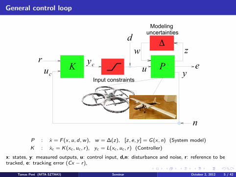
General control loop

K Pr

e

n

d

uc

Δ

Input constraints

Modeling uncertainties

ycu y

zw

P : x = F (x , u, d ,w), w = ∆(z), [z, e, y ] = G(x , n) (System model)

K : xc = K(xc , uc , r), yc = L(xc , uc , r) (Controller)

x: states, y: measured outputs, u: control input, d,n: disturbance and noise, r: reference to betracked, e: tracking error (Cx − r),


System models (P=?)

Linear Time-Invariant (LTI):

Time domain: x = Ax(t) + Bv(t)

y = Cx(t) + Dv(t), x(0) = x∗

Frequency domain (jω): G(jω) = C(jωI − A)−1B + D.If the Fourier transform v(jω) = F(v(t)) exists, then y(jω) = G(jω)v(jω) when x(0) = 0

S-domain (s): G(s) = C(sI − A)−1B + D.If the Laplace transform v(s) = L(v(t)) exists, then y(s) = G(s)v(s) when x(0) = 0

Convolution. Let δ(t) be the dirac delta defined as

δ(t) = 0, if t 6= 0 and

∫ ∞−∞

δ(t)dt = 1

The impulse response g(t) of the LTI system is the output if v(t) = δ(t) and x(0) = 0.g(t) is the inverse Laplace transform of G(s) For some u(t) the output can be expressed byusing g(t) as follows:

y(t) =

∫ t

0g(t − τ)v(τ)dτ


System models (P=?)

Linear Parameter-Varying (LPV)

x(t) = A(ρ(t))x(t) + B(ρ(t))v(t)

y(t) = C(ρ(t))x(t) + D(ρ(t))v(t),

ρ ≤ ρ(t) ≤ ρ, δ ≤ ρ(t) ≤ δ

Nonlinear, input-affine: x = f (x(t)) + g(x(t))v(t)

Stability: The origin is (exponentially) stable if x(t)→ 0 at exponential decay rate. This isequivalent to the existence of a positive definite Lyapunov function V (x(t)) > 0 satisfying

V (x(t)) < 0. For LTI systems

V (x) = xT Xx , X > 0 is enough and

the stability is equivalent to that the eigenvalues of A (or the poles of G(s)) are strictly inthe left half plane

Example Lyapunov stability. Let x = Ax be an autonomous, linear, time-invariant system. FromLyapunov theorem we know that it is stable is there exists a quadratic Lyapunov functionV (x) = xT Xx with X > 0, s.t. AT X + XA < 0. These conditions are equivalent to the followingLMI: (

X 00 −AT X − XA

)> 0


Signal spaces and operators


Signal spaces

Signal spaces: vector spaces of functions mapping the ’time axis’ T ⊂ R into a vector spaceV ⊂ Rn. Examples for T in case of continuous time systems are real numbers R = (−∞,∞) orR+ = (0,∞)

Normed (signal) space L: a linear vector space equipped with a norm ‖ · ‖

‖f ‖ = 0 ↔ f ≡ 0

‖αf ‖ = |α|‖f ‖‖f + g‖ ≤ ‖f ‖+ ‖g‖

If the normed space is complete, i.e. its Cauchy sequences converge, the normed space is calledBanach space. Examples for Banach spaces:

Lp [0,∞) : ‖f ‖p =

(∫ ∞0|fi |p dt

)1/p

Lp(−∞,∞) : ‖f ‖p =

(∫ ∞−∞|fi |p dt

)1/p

L∞[0,∞) : ‖f ‖∞ = ess supt∈R+

|f (t)|

where |f | is the standard Euclidean norm |f | = (f T f )1/2.


Signal spaces

Inner product space: linear vector space equipped with an inner product 〈·, ·〉 satisfying thefollowing properties (where f , g : T 7→ R and α ∈ R)

〈f , g〉 = 〈g , f 〉〈αf , g〉 = α〈f , g〉

〈f1 + f2, g〉 = 〈f1, g〉+ 〈f2, g〉

The inner product induces a norm:

‖f ‖ =√〈f , f 〉

If an inner product space is complete it is called Hilbert space. Hilbert spaces will be denoted byH to be distinguished from the normed spaces. Examples for Hilbert spaces:

Lm2 [0,∞) : 〈f , g〉 =

∫ ∞0

f (t)T g(t)dt =1

2π

∫ ∞−∞

f (jω)∗g(jω)dω

Lm2 (−∞,∞) : 〈f , g〉 =

∫ ∞−∞

f (t)T g(t)dt =1

2π

∫ ∞−∞

f (jω)∗g(jω)dω

where f (jω) is the Fourier transform of f (t). The examples show that, if p = 2 then Lp [0,∞)

and Lp(−∞,∞) are not only Banach but also Hilbert spaces.


Operators

Operators: mapping from one normed (signal) space into another. Now ’one=another’, i.e.H : L → L

Properties of operators:

Composition: H1H2 is also an operator defined by (H1H2)(f ) = H1(H2(f ))Sum: αH1 + βH2 is also an operator defined by (αH1 + βH2)(f ) = αH1(f ) + βH2(f )Linearity (we will assume it often): H(αf + βg) = αH(f ) + βH(g)Gain and boundedness:

‖H‖ = supf∈L,f 6=0

‖Hf ‖‖f ‖

<∞ (2)

Multiplicativity rule: ‖H1H2‖ ≤ ‖H1‖ · ‖H2‖

Example 1 (RH∞): Let x = Ax + Bu,y = Cx + Du, x(0) = 0 be a finite dimensional, linear,time-invariant (LTI) dynamical system with poles strictly in the left half plane. The LTI systemdefines an operator in terms of convolution

(Gu)(t) = (g ∗ u)(t) =

∫ t

0g(t − τ)u(τ)dτ G(s) = C(sI − A)−1B + D

where g(t) = L−1{G} is the weighting function (impulse response). Since all poles are stable,this operator is bounded on every on Lp [0,∞) space. (All poles on the left half plane is anecessary and sufficient condition for an operator to be bounded on Lp [0,∞) spaces. )


Operators

If we consider G as an operator on L2[0,∞) then its bound can be determined as follows:

‖G‖ = supf∈L2[0,∞),f 6=0‖Hf ‖‖f ‖

= supω∈[0,∞)

σmax (G(jω)) (the well-known H∞ norm)

If we consider G as an operator on L∞[0,∞) then its bound will be calculated as

‖G‖ = supf∈L∞[0,∞),f 6=0‖Hf ‖‖f ‖

=

∫ ∞0|g(t)| dt (i.e., the L1 norm of the impulse response)

Example 2 (RL∞): If the LTI system has poles both in the right and the left half plane, butthere is no pole on the imaginary axis, then G is a bounded operator on Lp [−∞,∞). Theoperator is defined in terms of convolution:

(Gu)(t) =

∫ ∞−∞

g(t − τ)u(τ)dτ (3)

where g(t) = L−1{G(s)} If G ∈ RL∞ is considered on L2[−∞,∞) then

‖G‖ = supω∈[0,∞]

σmax (G(jω))

Remark. The system norms can be computed in MATLAB by norm function.


Adjoint operators

Adjoint operators:Let H : H → H be a bounded linear operator. The Hilbert adjoint H∗ of H is the operatorH∗ : H → H s.t.

〈Hf , g〉 = 〈f ,H∗g〉 ∀f , g ∈ H

An operator is self-adjoint if H∗ = H. Examples:

Let H ∈ RH∞ be an operator with state space realization H(s) = C(sI − A)−1B + D.Then H∗(s) = H(−s)T = −BT (sI + AT )−1C T + DT . So, if H(s) stable then its adjointwill be unstable.

More generally, if H ∈ RL∞ then H∗(s) = H(−s)T .

Properties of Hilbert adjoint. The Hilbert adjoint H∗ exists uniquely and it is a linear operatorwith ‖H∗‖ = ‖H‖. Furthermore, for bounded operators H,H1,H2 : H → H the followingequations hold:

a) (αH)∗ = αH∗ b) (H1 + H2)∗ = H∗1 + H∗2 c) (H∗)∗ = Hd) (H1H2)∗ = H∗2 H∗1 e) ‖H∗H‖ = ‖HH∗‖ = ‖H‖2 f )(H∗)−1 = (H−1)∗


Self-adjoint operators and quadratic forms

Self-adjoint operators. A bounded linear operator H : H → H is self-adjoint if H∗ = H.

Remark. If H ∈ RH∞ and H is self-adjoint, then it is constant.

Quadratic forms.The quadratic form σ(f ) = 〈Hf , f 〉 defined by a self-adjoint operator H is positive semidefinite(positive definite) (denoted by H > (≥)0 if 〈Hf , f 〉 ≥ (>)0 for all f ∈ H.

Let Φ = Φ∗ : H → H. Then σ(f ) = 〈Φf , f 〉 is a quadratic form not only on H but also on its

subspace H ⊂ H. Φ ≥ 0 obviously implies that σ ≥ 0 on H , but the reverse implication is not atall clear. In the particular case when Φ = Φ∗ ∈ RL∞ and H = L2(−∞,∞), H = L2(0,∞) thenthe reverse implication holds, too:

σ(f ) ≥ 0 for all f ∈ L2[0,∞) ⇔ Φ(jω) ≥ 0 (4)

This makes it possible to define IQCs with noncausal Φ while the signals remain in L2[0,∞).


Methods for analyzing the stability of feedbackinterconnections


Extended spaces

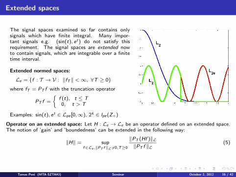
The signal spaces examined so far contains onlysignals which have finite integral. Many impor-tant signals e.g. (sin(t), et ) do not satisfy thisrequirement. The signal spaces are extended nowto contain signals, which are integrable over a finitetime interval.

Extended normed spaces:

Le = {f : T → V : ‖fT ‖ <∞, ∀T ≥ 0}

where fT = PT f with the truncation operator

PT f =

{f (t), t ≤ T0, t > T

Examples: sin(t), et ∈ Lpe [0,∞), 2k ∈ lpe (Z+)

Operator on an extended space: Let H : Le → Le be an operator defined on an extended space.The notion of ’gain’ and ’boundedness’ can be extended in the following way:

‖H‖ = supf∈Le ,‖PT f ‖L 6=0,T≥0

‖PT (Hf )‖L‖PT f ‖L

(5)


Causality

Causality: the value at a certain time does not depend on future values of the argument

PTHPT = PTH, ∀T ∈ T

Anticausality: the future matters only, i.e. (I − PT )H = (I − PT )H(I − PT )

An important consequence of causality: If an operator is causal then it is bounded onLe if and only if it is bounded on L and the gain defined over the two signal spaces (Le

and L) are equal:

‖H‖ = supf∈Le ,‖PT f ‖L 6=0,T≥0

‖PT (Hf )‖L‖PT f ‖L

= supf∈L,f 6=0

‖Hf ‖L‖f ‖L

This lemma enables us to use the L2-space, instead of the extended L2e during thestability analysis.


Elementary system properties

H 2

H 1

u2

e1u1

e2

-

H1,H2 are operators on normed space Le .

Well-posedness: the interconnection makes sense, that is the system does not have finite escapetime, u uniquely determines e and the mapping u 7→ e is causal.

Example1: Let H1(s) = 1/(s + 1), H2(x) = −x − x2, u1(t) = θ(t) (unit step function), u2 = 0.Then the closed loop realizes the differential equation x = x2 + 1. The solution isx(t) = tan(t)θ(t), which goes to infinity if t → π/2. This means the closed loop has finiteescape time so it is ill-posed.

Example2: Let H1 = 1, H2(x) = e−sT − 1, u2 = 0. Then the closed loop realizes the mappingy(t) = u1(t + T ), so the closed loop is not causal.

Definition. The interconnection is well-posed if for any u1, u2 ∈ Le there exists a solutione1, e2 ∈ Le and they depend causally on u1 and u2.

Stability: A well-posed system is stable if there exists c1, c2, c3, c4 s.t.

‖e1T ‖ ≤ c1‖u1T ‖+ c2‖u2T ‖‖e2T ‖ ≤ c3‖u1T ‖+ c4‖u2T ‖

where eiT = PT ei .


Integral Quadratic Constraints

Δ

G

e

w0

v

+

S 1 :

G : LTI transfer function defining a bounded, causaloperator on the extended Hilbert-space He

∆: bounded, causal operator on the same He space.

We particularly interested in the special case whenHe = L2e [0,∞)

Integral Quadratic Constraint (IQC). Let Π be a bounded, self-adjoint operator. Then we say,∆ satisfies the IQC defined by Π (∆ ∈ IQC(Π)) if

σΠ(v ,∆(v)) =

⟨[v

∆(v)

],Π

[v

∆(v)

]⟩≥ 0 ∀v ∈ L2[0,∞)

We call Π the multiplier that defines the IQC. (Note that the IQC is defined on L2 even thoughthe operators are defined on the extended L2e space.)

Remark. If ∆ ∈ IQC(Π1) and ∆ ∈ IQC(Π2) then ∆ ∈ IQC(τ1Π1 + τ2Π2), τi ≥ 0.

Remark. Since we defined the IQC over L2[0,∞) space, Π can be taken as a transfer functionΠ(jω) = Π(jω)∗. The condition above then reduces to

σΠ(v ,∆(v)) =

∫ ∞−∞

[v(jω)ˆ∆(v)(jω)

]∗Π(jω)

[v(jω)ˆ∆(v)(jω)

]≥ 0, ∀ v ∈ L2[0,∞)


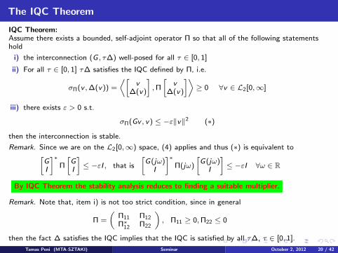
The IQC Theorem

IQC Theorem:Assume there exists a bounded, self-adjoint operator Π so that all of the following statementshold

i) the interconnection (G , τ∆) well-posed for all τ ∈ [0, 1]

ii) For all τ ∈ [0, 1] τ∆ satisfies the IQC defined by Π, i.e.

σΠ(v ,∆(v)) =

⟨[v

∆(v)

],Π

[v

∆(v)

]⟩≥ 0 ∀v ∈ L2[0,∞]

iii) there exists ε > 0 s.t.

σΠ(Gv , v) ≤ −ε‖v‖2 (∗)

then the interconnection is stable.

Remark. Since we are on the L2[0,∞) space, (4) applies and thus (∗) is equivalent to[GI

]∗Π

[GI

]≤ −εI , that is

[G(jω)

I

]∗Π(jω)

[G(jω)

I

]≤ −εI ∀ω ∈ R

By IQC Theorem the stability analysis reduces to finding a suitable multiplier.

Remark. Note that, item i) is not too strict condition, since in general

Π =

(Π11 Π12

Π∗12 Π22

), Π11 ≥ 0,Π22 ≤ 0

then the fact ∆ satisfies the IQC implies that the IQC is satisfied by all τ∆, τ ∈ [0, 1].


System analysis by using IQCs


The closed loop system

K

ΔmW m(s)

Pr e

n

d

W e(s)

W u(s) u p

u

ΔaW a(s)

1 Nominal model P, defining an LTI causal and bounded operator.

2 Controller. We assume that the controller has already been designed so it is known now.

3 External inputs. Inputs coming from the environment. They can be disturbances, sensor- oractuator noises. The reference signal, which has to be tracked by the output of the plant, isalso an external signal. The external signals are assumed to come from some extendedHilbert space He . Typically He = L2e [0,∞).IQCs can also be used to formulate the properties of the external signals:

σΨ(d) =

∫ ∞−∞

d(jω)∗Ψ(jω)d(jω)dω ≥ 0

holds for input d ∈ L2[0,∞] with some Ψ ∈ RL∞ then this property can be taken intoaccount during the analysis procedure.

4 Performance outputs. Inner signals or outputs, the behavior of which are important for us.They can also be weighted - We (s),Wu(s)



K

ΔmW m(s)

Pr e

n

d

W e(s)

W u(s) u p

u

ΔaW a(s)

5 Nonlinear elements and time delays. The nonlinear components can either be static (e.g.saturations, deadzones) or dynamic (e.g. friction).

6 Uncertainty. Models the difference between the mathematical model and the real system.Uncertainty can be present due to approximation or identification errors, change ofparameters and nonlinearities due to wear or change of operating conditions. Typicaluncertainty models:

LTI Dynamic uncertainty. It represents unmodeled dynamics or model error fromidentification. It is defined by an unknown, stable transfer function with bounded H∞norm. Typically, ‖∆‖H∞ ≤ 1 and W (s) weighting function is applied to describe thefrequency distribution of the uncertainty. It can be inserted into the system either byadditive or multiplicative structure.Parametric uncertainty. It is used to model uncertain gain, uncertainty in the locationof poles or zeros or unknown changes in physical parameters.Polytopic uncertainty. Special class of parametric uncertainty. The possible parametervalues come from a convex polytope:

p(t) ∈ ∆ = {p | p =∑

i

λi pi , λ1 ≥ 0,∑

i

λi = 1, i = 1, . . . ,N}Tamas Peni (MTA-SZTAKI) Seminar October 2, 2012 23 / 42


K

ΔmW m(s)

Pr e

n

d

W e(s)

W u(s) u p

u

ΔaW a(s)

The aim of the analysis is to check whether the system satisfy the robust performance criterium.Robust performance comprises the following two conditions:

robust stability. The system has to be stable for all possible values of uncertainties,nonlinearities, delays, etc.

performance. The performance outputs should satisfy the prescribed specification. Theperformance is generally formalized by a quadratic relation, e.g.

σP (zP ,wP ) =

∫ ∞0

[zP (t)wP (t)

]T

P

[zP (t)wP (t)

]dt ≤ 0, zP ,wP ∈ L2[0,∞)

Important performance measure: the induced L2-norm (i.e the H∞ operator norm in LTIcase):

‖zP‖L2

‖wP‖L2

≤ γ ⇒ σP (zP ,wP ) =

∫ ∞0

[zP (t)wP (t)

]T [γ−1I 0

0 −γI

] [zP (t)wP (t)

]dt ≤ 0


LFT representation

The first step of analysis is pulling out the unknown and nonlinear blocks:

wP=[ rnd ]

Δm

G

Δ

zP=[ eu p ]

GwP=[ rnd ] zP=[ eu p ]

Δ

Δm

z

zw

w

Upper LFT: zP = Fu(G ,∆)wP = [G22 + G21∆(I − G11∆)−1G12]wP (left)

Lower LFT: zP = Fl (G ,∆)wP = [G11 + G12∆(I − G22∆)−1G21]wP (right)


System analysis by using IQCs

STEP 1.

1 Construct a suitable, linearly parameterized set of IQCs for each uncertain, nonlinear block.

∆k ∈ IQC(Πk (λΠk)), for all λΠk

∈ ΛΠk

Build one diagonal IQC, that is satisfied by the augmented block ∆ = diag(∆1, . . . ,∆N ):

∆ ∈ IQC(Π(λΠ)), Π(λΠ) = diag(Π1(λΠ1), . . . ,ΠN (λΠN

)), λΠ = (λ1, . . . , λN )

The IQC defines quadratic inequality condition between w and z : σΠ(λΠ)(z,w) ≥ 0

2 You may choose (linearly parameterized) IQC conditions for the external inputs:σΨ(λΨ)(wP ) ≥ 0

3 Prescribe the performance requirements by using IQC: σP(γ)(zP ,wP ) ≤ 0


S-procedure

S-procedure. Let σk : H → R be quadratic forms defined as

σk (f ) = 〈Φk f , f 〉, k = 0, 1, . . . ,N

where Φk are linear, bounded, self-adjoint operators on H. We consider the following twoproblems:

S1 : σ0(f ) ≤ 0 for all f ∈ H s.t. σk (f ) ≥ 0, k = 1, . . . ,N.

S2 : there exists τk ≥ 0, k = 1, . . . ,N, such that

σ0(f ) +N∑

k=1

τkσk (f ) ≤ 0, ∀f ∈ H

It is obvious that S2 implies S1. The opposite direction holds only in special cases.

STEP 2.

The interconnection satisfies the robust performance requirements if there exist λΠ, λΨ s.t.

σP(γ)(G21w + G22wP ,wP ) + σΠ(λΠ)(G11w + G12wP ,w) + σΨ(λΨ)(wP ) < 0

which, over the L2[0,∞) space, is equivalent to the frequency domain inequality:[G(jω)

I

]∗Π(jω)

[G(jω)

I

]< 0, ∀ω ∈ [0,∞]

where Π(jω) collects all multipliers Π(λΠ),Ψ(λΨ),P(γ) and thus depends on λΠ, λΨ, γ.


Transforming frequency domain inequalitis to LMI

We want to check the feasibility of[G(jω)

I

]∗Π(jω)

[G(jω)

I

]< 0, ∀ω ∈ [0,∞]

Let

Π =

[(jωI − Aπ)−1Bπ

I

]∗Mπ


I

]where Bπ = [Bπ,v Bπ,w ] and Aπ is stable. For simplicity, the dependence of Π(jω) on λ isomitted. Then we have[

(jωI − Aπ)−1BπI

]·[

G(jω)I

]∗Mπ


I

]·[

G(jω)I

]< 0

To perform the multiplications we use the following lemma:

If Gi (s) = Ci (sI − Ai )−1Bi + Di =

[Ai Bi

Ci Di

]then

G1G2 =

A1 B1C2 B1D2

0 A2 B2

C1 D1C2 D1D2


Transforming frequency domain inequalitis to LMI

Then we find that the original inequality can be formulated as[(jωI − A)−1B

I

]∗ [Q S

ST R

] [(jωI − A)−1B

I

]> 0 (�)

where

A =

[Aπ Bπ,v CG

0 AG

], B =

[Bπ,v DG + Bπ,w

BG

]and [

Q SST R

]= −

I 0 00 CG DG

0 0 I

T

Mπ

I 0 00 CG DG

0 0 I

From (4) it follows that (�) is equivalent to the existence of ε > 0 s.t.

ε‖w‖2 ≤∫ ∞−∞

[(jωI − A)−1Bw(jω)

w(jω)

]∗ [Q S

ST R

] [(jωI − A)−1Bw(jω)

w(jω)

](6)

=

∫ ∞0

(xT Qx + 2xT Sw + wT Rw)dt (7)

for all pairs (x ,w) ∈ L2[0,∞), where x = Ax + Bw , x(0) = 0, w ∈ L2[0,∞). This is a

linear-quadratic optimal control problem.


Kalman-Yakubovic-Popov Lemma

The following statements are equivalent:

there exist of ε > 0 s.t.∫ ∞0

(xT Qx + 2xT Sw + wT Rw)dt ≥∫ ∞

0|x |2 + |w |2dt

for all pairs (x ,w) ∈ L2[0,∞), where x = Ax + Bw , x(0) = 0, w ∈ L2[0,∞).

we have[(jωI − A)−1B

I

]∗ [Q S

ST R

] [(jωI − A)−1B

I

]> 0 ∀ω ∈ [0,∞)

there exists P = PT s.t.

[PA + AT P PB

BT P 0

]+

[Q S

ST R

]> 0 LMI condition!

Linear dependence of Π(jω) on the parameters λ = (λΠ, λΨ, γ) is generally shifted into Mπ(λ),which results in parameter dependent Q(λ), S(λ) and R(λ).


List of IQCs


LTI uncertainty

1. D-scaling:

Let ∆ = diag(∆1, . . . ,∆m) LTI operator with norm ‖∆i‖∞ ≤ 1. In frequency domain we canchoose an IQCwith multiplier

Π(jω) =

[−D(jω)∗D(jω)

D(jω)∗D(jω)

]s.t. ∆D = D∆

where D(jω) is a free variable. Since(I∆

)∗ [D(jω)∗D(jω)

−D(jω)∗D(jω)

](I∆

)= −∆∗D∗D∆ + D∗D = D∗[I −∆∗∆]D > 0

The condition of stability in this special case can be given as follows(GI

)∗ [D(jω)∗D(jω)

−D(jω)∗D(jω)

](GI

)= −D∗D + G∗D∗DG < 0 ⇔ ‖DGD−1‖ < 1

This is the D-iteration part of the D-K iteration used in robust control design. The design ofscaling D(jω) is a construction of a suitable multiplier.


Polytopic uncertainty

2. Time-varying, causal, linear, structured uncertainty:

(∆z)(t) = ∆(t)z(t), ∆(t) = diag(δ1(t)I , . . . , δm(t)I ) |δi (t)| ≤ 1 for t ≥ 0. Then

Π =

{(Q ST

S R

)| R = −Q, Q = diag(Q1, . . . ,Qm) > 0,

S = diag(S1, . . . ,Sm), Sj + STj = 0

}

3. Time-varying, causal, linear, polytopic un-certainty:

(∆z)(t) = ∆(t)z(t), ∆(t) ∈ co{∆1, . . . ,∆N},∆i ∈ Rn×n. Then

Π =

{(R ST

S Q

)| Q < 0,

(I

∆j

)T

Π

(I

∆j

)}Δ1

Δ(t)

Δ2

Δ(t)=∑1

m

α jΔ j

∑1

m

α j=1,α j≥0

Δm−1

Δm


Sector bounded nonlinearities

4. Memoryless nonlinearity in a sector

Let w(t) = (∆z)(t) = φ(z(t), t)) : R× R→ R be afunction contained in a sector [α, β], i.e.

αz2 ≤ φ(z, t)z ≤ βz2, ∀z ∈ R, t ≥ 0

φ( z)β z

α z

Then βz − φ(z, t) and φ(z, t)− αz have the same sign, that is (βz − φ(z, t))(φ(z, t)− αz) ≥ 0.This implies the following constant multiplier:

Π(jω) =

[−2αβ α+ βα+ β −1

](8)

5. The ”Popov” IQCIf w(t) = (∆z)(t) = φ(z(t)) : R→ R be a continuous function, z(0) = 0 and both w(·) and z(·)are square summable, then

∫∞0 z(t)w(t) = 0 holds. This implies in frequency domain the

following IQC:

Π(jω) = ±[

0 jωλ−jωλ 0

], λ ∈ R (9)

Note that, this multiplier is not proper, so in general it is combined with other multipliers orinstead of ∆, the modified ∆ = ∆ ◦ 1

s+1is considered. The modified (proper) multiplier is

Π(jω) = ±[

0 jω1+jω

λ

− jω1+jω

λ 0

], λ ∈ R

Remark. The sum of (8) and (9) gives the Popov criterion for memoryless, sector bounded,continuous nonlinearities.


Slope restricted nonlinearities

Let w(t) = (∆z)(t) = φ(z(t)) : R → R be a staticnonlinearity with the following properties:

i) φ(0) = 0

ii) With some α ≤ β

α ≤φ(z1)− φ(z2)

z1 − z2≤ β

iii) there exists k > 0 s.t. |φ(z)| ≤ k|z|

φ(z)

β z

α z

6. Zames-Falb multiplier [Zames,Falb 1968]:The following multiplier was derived by Zames and Falb in [Zames,Falb 1968]:

Π(jω) = T T

[0 1 + H(jω)∗

1 + H(jω) 0

]T

where H is a strictly proper rational transfer function with impulse response h and the followingconstraints are satisfied:

h(t) ≤ 0 for all t ∈ R. If φ is an odd function then this constraint is not needed.

L1-norm constraint: ‖h‖1 =∫∞−∞ |h(t)|dt ≤ 1

T =

[ ββ−α − 1

β−α− α 1

]Tamas Peni (MTA-SZTAKI) Seminar October 2, 2012 35 / 42

Slope restricted nonlinearities

Sketch of proof : We prove only the special case, when φ is odd and β = 1, α = 0. The normedsaturation nonlinearity satisfies these properties.

Since |v(t)| ≥ |ϕ(v(t))| and |ϕ(v(t))| ≥ |h ∗ ϕ(v(t))| thus

[v(t)− ϕ(v(t))] · [ϕ(v(t)) + (h ∗ ϕ(v(t)))] ≥ 0

Consequently

0 ≤∫ ∞

02[v − ϕ(v)] · [ϕ(v) + h ∗ ϕ(v)]dt =∫ ∞−∞

2Re[v(jω)− ϕ(v)(jω)]∗[ϕ(v)(jω) + H(jω)ϕ(v)(jω)]dω

=

(v(jω)

ϕ(v)(jω)

)∗ [0 1 + H(jω)

1 + H(jω)∗ −2(1 + ReH(jω))

](v(jω)

ϕ(v)(jω)

)

Remark 1. The filter H can be non-causal (poles on the right half plane!). The construction of H

is not easy, only approximate solutions exist. E.g. [Chen and Wen, 1995]


Beyond the analysis


Controller synthesis

wP

Δm

G zP

zw

K

yu

Π=?

K=?

Analysis ≡ find a multiplier

Synthesis ≡ find a multiplier

and a controller

so that the closed-loop satisfies the robust perfor-mance.

The synthesis cannot be transformed to a convexoptimization problem.

Iterative design is needed: the multiplier and the con-troller are tuned alternately until the performance re-quirements are met.

convergence cannot be guaranteed in general

numerical problems

problem-specific solvers are needed


Linear Parameter-Varying (LPV) systems

Useful extension of the LTI dynamics:

x(t) = A(ρ(t))x(t) + B(ρ(t))u(t), y = C(ρ(t))x(t) + D(ρ(t))u(t)

where ρ(t) ∈ Rp is the measured, time-varying scheduling parameter, which has in general,

well-known magnitude and rate bounds: ρi≤ ρi (t) ≤ ρi , δi ≤ ρi (t) ≤ δi .

Properties:

good modeling capabilities - by letting ρ(t) = f (x(t)) the nonlinear behavior can beembedded into the LPV structure

powerful analysis and design tools of LTI system theory remain applicable

Controller synthesis:

wP G (s) zP

zw

K (s)

yu

ρ

wP G (s) zP

zw

K (s)

yu

Φ(ρ)

ρ

Φ(ρ)

wP G (s ,ρ) zP

K (s ,ρ)

yu


Beyond the IQCs(Hard constraints in control)


Set-theoretic methods

Hard constraints:

u(t) ∈ U, x(t) ∈ X X ,U are convex sets, polytopes

These constraints cannot be handled by IQCs! Different approach is needed!

The problem seems easier in discrete-time:

x = Acx(t) + Bcu(t) + Ecd(t) ⇔ZOH x(k + 1) = Ax(k) + Bu(k) + Ed(k)

A = eATs , [B E ] =

∫ Ts

0

eA(t−τ)[Bc Ec ]dτ

1 If Ac is not stable and u is subject to hard constraints the system can be stabilizedonly on a closed set of states. How can this set be determined?

2 If Ac is stable and d(k) ∈ D and D is convex (polytope) then the states converge toa closed set around the origin. This is the minimal disturbance invariant set. Howdoes it look like?

3 The maximal disturbance invariant set contained in X is the maximal subset of X ,which cannot be leaved by the trajectories of the system in the presence ofconstrained disturbance d(k) either. How can this set be computed efficiently?


Examples

Maximal disturbance invariant set Minimal disturbance-invariant set.contained in X

Problems: numerical difficulties, exponentially growing complexity, increasing number of verticesProblem to be solved: find at each step the best inner and outer approximation by using onlyfixed number of vertices.


analysis of systems containing nonlinear and uncertain

Documents