analysis of the general image quality equation - the institute of optics

Analysis of the general image quality equation Samuel T. Thurman and James R. Fienup

The Institute of Optics, University of Rochester, Rochester, NY 14627

ABSTRACT

The general image quality equation (GIQE) [Leachtenauer et al., Appl. Opt. 36, 8322-8328 (1997)] is an empirical formula for predicting the quality of imagery from a given incoherent optical system in terms of the National Imagery Interpretability Rating Scale (NIIRS). In some scenarios, the two versions of the GIQE (versions 3.0 and 4.0) yield significantly different NIIRS predictions. We compare visual image quality assessments for simulated imagery with GIQE predictions and analyze the physical basis for the GIQE terms in an effort to determine the proper coefficients for use with Wiener-filtered reconstructions of Nyquist and oversampled imagery in the absence of aberrations. Results indicate that GIQE 3.0 image quality predictions are more accurate than those from GIQE 4.0 in this scenario.

Keywords: Image quality assessment, resolution, image restoration

1. INTRODUCTIONThe National Imagery Interpretability Rating Scale (NIIRS) is a quantitative task-based scale for image quality [1,2] used for military, civilian, and agricultural applications. The scale ranges from 0, representing the poorest quality, to 9, representing the highest quality, where each unit on the NIIRS scale is worth a factor of two in resolution [1,2]. A change of 0.1 is barely noticeable by a human observer, while a change of 0.2 is easily perceived [3]. The general image quality equation (GIQE) is an empirical formula for calculating the image quality that can be expected from a given optical system [2]. The GIQE is useful to optical engineers for designing new systems to meet specified NIIRS performance requirements, performing system trade studies [3,4], and efficiently tasking existing optical systems to achieve desired levels of image quality. Attempts to apply the GIQE to imaging scenarios unrepresented in the original regression analysis, however, have been unsuccessful [5,6]. Here we examine the physical basis of GIQE terms in an effort to better understand these limitations and determine the proper coefficients for use with imagery sampled at or above the Nyquist rate, which was unrepresented in the derivation of previous GIQEs.

2. GENERAL IMAGE QUALITY EQUATION The two versions of the GIQE (versions 3.0 and 4.0) have the following form

0 1 10 2 10 3 4GNIIRS log GSD log RER H

SNRc c c c c , (1)

where c0, c1, c2, c3,and c4 are coefficients with values listed in Table 1, GSD is the system ground sample distance, RER is the system post-processing relative edge response, G is the system post-processing noise gain, SNR is the signal-to-noise ratio of the unprocessed imagery, and H is the system post-processing edge overshoot factor, all of which are defined in Refs. [1,2]. In this paper, a generalized definition of H [Eq. (18) in Section 4.4] is used. The GIQE essentially accounts for three factors that affect image utility: (i) spatial resolution (GSD and RER are measures of the system spatial resolution), (ii) noise (G /SNR is a measure of the noise in the post-processed imagery, but SNR also affects RER when using the Wiener filter), and (iii) artifacts (H is a measure of the amount of edge ringing resulting from post-processing). Other factors, such as image brightness, contrast, and scale, are not accounted for in the GIQE, because these attributes are assumed to be optimized when each image is displayed [2].

Table 1. GIQE versions 3.0 and 4.0 coefficients.

c0 c1 c2 c3 c4

GIQE 3.0 11.81 –3.32 3.32 –1 –1.48 GIQE 4.0 (for RER 0.9) 10.251 –3.32 1.559 –0.334 –0.656 GIQE 4.0 (for RER < 0.9) 10.251 –3.16 2.817 –0.334 –0.656

Visual Information Processing XVII, edited by Zia-ur Rahman, Stephen E. Reichenbach, Mark Allen Neifeld, Proc. of SPIE Vol. 6978, 69780F, (2008) · 0277-786X/08/$18 · doi: 10.1117/12.777718

Proc. of SPIE Vol. 6978 69780F-1

The GIQE can be used to predict the resulting change in image quality in terms of NIIRS when various system parameters are adjusted, where

GSD RER G SNR H

0

NIIRS NIIRS NIIRS NIIRS NIIRS

NIIRS NIIRS , (2)

GSD 1 100

GSDNIIRS logGSD

c , (3)

RER 2 100

RERNIIRS logRER

c , (4)

0G SNR 3

0

GGNIIRSSNR SNR

c , (5)

H 4 0NIIRS H Hc , (6)

and the 0 subscript represents quantities corresponding to a reference baseline image.

Table 2 lists the characteristics of the set of 359 images used for the derivation and validation of GIQE 4.0. Reference [2] mentions that the GSD and RER terms are the dominant terms and that the G/SNR and H terms have much less of an influence in determining image quality. The sampling ratio for all of the imagery was Q = f / (D p) = 1, where

is the wavelength of light, f is the system focal length, D is the system pupil diameter, and p is the detector pixel pitch. Reference [2] notes that GIQE 4.0 may not be valid for Q > 1. Futhermore, it is assumed that all of the imagery was obtained with well-corrected optical systems having an annular pupil with a fairly large fill factor.

Table 2. Characteristics of imagery used for derivation and validation of GIQE 4.0*.

Minimum Mean Maximum

GSD 3 in. 20.6 in. 80 in. RER 0.2 0.92 1.3 G 1 10.66 19 SNR 2 52.3 130 G/SNR 0.01 – 1.8 H 0.9 1.31 1.9 *Data taken from Ref. [2].

Published attempts to extrapolate GIQE 4.0 to imagery with parameters unrepresented in the original regression analysis have not been successful. Reference [5] found that GIQE 4.0 predictions were inaccurate for SNR 3. Additionally, GIQE 4.0 has been shown to be inaccurate for imagery from sparse-aperture systems [6]. In the following sections, we attempt to determine the appropriate GIQE coefficients for Wiener-filtered imagery with Q 2, based on human evaluation of simulated imagery and physics-based arguments.

3. SIMULATED IMAGERY Figure 1 is a portion of a digital Snellen eye chart that was used as an object for the simulated imagery. This object was chosen because it is applicable to task-based assessment by untrained human observers, where the task is simply to correctly identify the text. This avoids the costly process of having professional image analysts evaluate each image. Additionally, the systematic variation in the font size within the eye chart permits a visual determination of the spatial resolution an image in terms of the minimum readable font size. The sampling for the object is a factor of ~7.5 finer than finest GSD for the simulated imagery. The dark letters on the eye chart represent areas of 7% reflectance, while the reflectance of the bright background is 15%.


PDCLPED

- PECFD- EDFCZP

FELOPZDDEFPOTEC

LEFODPCT rnL?ozrcpFDPLTCEQ kPCFCTOOZ

Fig. 1. Digital object used for image simulations (not shown at full resolution). For later reference, the point sizes of the font in each row are (top to bottom): 60, 50, 40, 30 25, 20, 15, 13, 10, 8, 6, 5, and 4 pt.

Fig. 2. Baseline image with GSD0 = 1 (arbitrary units), Q0 = 2, and SNR0 = 500. The inset contains a magnified portion of

the image with text lines having font sizes comparable to the spatial resolution limit of the image.

Figure 2 is a baseline image obtained by Wiener filtering [7-10] a simulated image from an unaberrated circular-aperture system with ground sample distance GSD0 = 1 (arbitrary units), sampling ratio Q0 = 2 (Nyquist sampling), and signal-to-noise ratio SNR0 = 500 (high SNR regime). The Wiener filter is implemented in the Fourier domain as

*

2n o

,,

, ,

S u vW u v

S u v c u v, (7)

where u and v are spatial frequency coordinates, W(u,v) is the Wiener filter, S(u,v) is the transfer function of the imaging system, c = 0.2 is a Wiener filter parameter, n is the noise spatial power spectrum (the noise is assumed to be white in the Fourier domain), and o(u,v) is the object spatial power spectrum, which is modeled [11,12] as


20

o 2 2

0,

0

Au v

A, (8)

where is the radial spatial frequency coordinate and A0, A, and are model parameters determined numerically from the digital object shown in Fig. 1. Visually, the spatial resolution (in terms of the minimum readable font size) for the image in Fig. 2 is determined to be 4-5 pt, depending on the criterion used to determine the resolution limit (all of the 5 pt letters can be correctly identified in the image, whereas only a fraction of the 4 pt letters can be identified).

A number of different images were simulated by varying the system GSD, Q, or SNR. Figure 3 shows three images from a sequence with image quality degraded by increasing GSD with fixed parameters Q = Q0 and SNR = SNR0. In this scenario, both the pixel and optical resolution of the system scale with GSD. This scaling is confirmed by visual assessment of the minimum resolvable font sizes being 8-10 pt, 15-20 pt, and 30-40 pt for the GSD = 2 GSD0, 4 GSD0and 8 GSD0 images, respectively.

Figure 4 shows three images from an image sequence with increasing Q and fixed values of GSD = GSD0 and SNR = SNR0. In this situation, the spatial resolution of the imagery is limited by the optical resolution of the system. Using a resolution measure that is proportional to the inverse of the diffraction-limited spatial frequency cutoff, the image resolution should scale with 1/Q for Q 2. Visual assessment of the minimum resolvable font size for the images shown in Fig. 4 agrees with this expectation. Comparison of Figs. 3 and 4 show that increasing GSD holding Q = 2 and increasing Q 2 holding GSD fixed have comparable image quality (ability to recognize letters) as one might expect.

Figure 5 shows three images from an image sequence degraded by reducing SNR with GSD = GSD0 and Q = Q0.Note that the primary effect on image quality of a low SNR is to reduce the net system resolution after Wiener filtering. Additionally, the increased noise amplitude and spatial correlation of the noise resulting from the Wiener filter [13-16] degrade image quality. The SNR values were chosen to yield NIIRS values (according to GIQE 3.0) of –1.0, –2.0 and –3.0 for the images shown in Figs. 5(a), 5(b), and 5(c), respectively. Based on visual assessment, the image quality of Figs. 5(b) and 5(c), however, appears to be worse than the GIQE 3.0 prediction, i.e., the minimum readable font size in Fig. 5(b) is 20-25 pt compared with 15-20 pt expected for NIIRS = –2.0, and the 50 and 60 pt font sizes in Fig. 5(b) are barely legible when 30-40 pt font size should be legible for NIIRS = –3.0. GIQE 4.0 predictions are in even worse agreement with visual observations (the corresponding NIIRS predictions are –0.8, –1.6, and –2.6 for each of the images in Fig. 5 according to GIQE 4.0).

4. GIQE ANALYSIS 4.1 Ground sample distance

In the geometric optics limit, the resolution of an unaberrated optical system is determined by the detector pixel width, which is proportional to the GSD. Assuming that the optical resolution of the system scales with the detector pixel width (in practice this is usually true by design) and the influence of noise and artifacts are constant (or negligible), the image quality can be expected to vary with GSD as

02 10

0

GSD GSDNIIRS log 3.32 logGSD GSD

, (9)

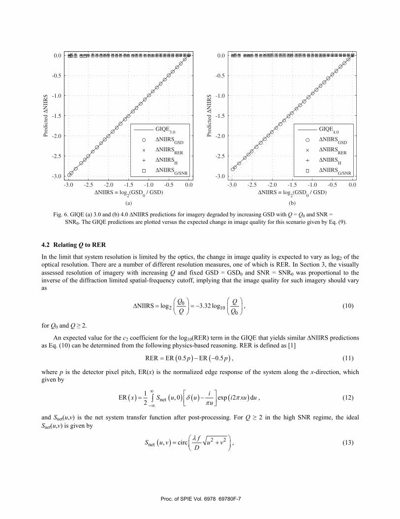
suggesting a value of c1 = –3.32 for the log10(GSD) in the GIQE [compare with Eq. (3)]. This embodies the notion that NIIRS changes by 1.0 for each factor of two of resolution change. Note that this relationship was confirmed by visual observations as described in Section 3. Figure 6 shows the variation in image quality predicted by GIQE 3.0 and 4.0 for an image sequence degraded by varying GSD with fixed values of Q = Q0 and SNR = SNR0. In this scenario, the RER, G/SNR, and H terms remain constant as GSD changes (the small fluctuations of these terms visible in Fig. 6 are artifacts resulting from the numerical evaluation of these terms). The GIQE predictions are plotted as functions of the expected change in image quality given by Eq. (9). Thus, the GIQE NIIRS predictions will fall on a unit-slope line passing


pDc

(a)

PDC- LPED- PECfl

EDFd

-PDC- LPED- PECFD- EDFCZP

rDPLTttOPtEOLCIVD

-. FELO EDL'OirCP — tLOPZD-- DEPPO — DtIPOTCC

LCFODPCT — t*IORL?rDPLrctol

—ø ptao&on. —

(a) (b)

PDCI. P CDrtCrDisits.— _ — — —•ise.I• SI•....— -

— S.— —

(c)

Fig. 3. Images degraded by increasing GSD with Q = Q0 and SNR = SNR0: (a) GSD = 2 GSD0, (b) GSD = 4 GSD0, and (c) GSD = 8 GSD0.

Fig. 4. Images degraded by increasing Q with GSD = GSD0 and SNR = SNR0: (a) Q = 2 Q0, (b) Q = 4 Q0, and (c) Q = 8 Q0.


PDC- LPED-- PEC1'- EDFd

putLPEDPECFD1. I P !

I r C I I

FELODEFPO____

LEr0OPcTropI.Tc,.o

(a)

U)YLPQPZD•..tf-9.ttc.tzflkpPat

— S.. i$tt* .H

(b)

I-

td r1

_ H(c)

Fig. 5. Images degraded by reducing SNR with GSD = GSD0 and Q = Q0: (a) SNR = 6.54 = SNR0 / 76, (b) SNR = 1.29 = SNR0 / 386, and (c) SNR = 0.25 = SNR0 / 1966.

through the origin of each graph if they agree with the expected changes image quality. The GIQE 3.0 predictions agree with our expectations since c1 = –3.32, while the GIQE 4.0 predictions are off slightly due to the fact that c1 = –3.16 (RER = 0.87). Reference [2] notes that the empirical relationship between NIIRS and GSD was observed to vary with RER for the imagery used to derive GIQE 4.0 and that a coefficient of c1 = –3.16 provided a better fit to the data than c1= –3.32 for RER < 0.9. The physical basis for this is unknown.


∆NIIRS = log2(GSD

0 / GSD)

Pred

icte

d∆

NII

RS

GIQE4.0

∆NIIRSGSD

∆NIIRSRER

∆NIIRSH

∆NIIRSG/SNR

-3.0 -2.5 -2.0 -1.5 -1.0 -0.5 0.0

-3.0

-2.5

-2.0

-1.5

-1.0

-0.5

0.0

∆NIIRS = log2(GSD

0 / GSD)

Pred

icte

d∆

NII

RS

GIQE3.0

∆NIIRSGSD

∆NIIRSRER

∆NIIRSH

∆NIIRSG/SNR

(a) (b)

-3.0 -2.5 -2.0 -1.5 -1.0 -0.5 0.0

-3.0

-2.5

-2.0

-1.5

-1.0

-0.5

0.0

Fig. 6. GIQE (a) 3.0 and (b) 4.0 NIIRS predictions for imagery degraded by increasing GSD with Q = Q0 and SNR = SNR0. The GIQE predictions are plotted versus the expected change in image quality for this scenario given by Eq. (9).

4.2 Relating Q to RER

In the limit that system resolution is limited by the optics, the change in image quality is expected to vary as log2 of the optical resolution. There are a number of different resolution measures, one of which is RER. In Section 3, the visually assessed resolution of imagery with increasing Q and fixed GSD = GSD0 and SNR = SNR0 was proportional to the inverse of the diffraction limited spatial-frequency cutoff, implying that the image quality for such imagery should vary as

02 10

0NIIRS log 3.32 log

Q QQ Q

, (10)

for Q0 and Q 2.

An expected value for the c2 coefficient for the log10(RER) term in the GIQE that yields similar NIIRS predictions as Eq. (10) can be determined from the following physics-based reasoning. RER is defined as [1]

RER ER 0.5 ER 0.5p p , (11)

where p is the detector pixel pitch, ER(x) is the normalized edge response of the system along the x-direction, which given by

net1ER , 0 exp 2 d2

ix S u u i xu uu

, (12)

and Snet(u,v) is the net system transfer function after post-processing. For Q 2 in the high SNR regime, the ideal Snet(u,v) is given by

2 2net , circ fS u v u v

D, (13)


where circ( ) = 1 for 1 and 0 otherwise. Substituting Eqs. (12) and (13) into Eq. (11) and simplifying yields

c

0RER 2 sinc d

up pu u , (14)

where uc = D / f = 1 / (p Q) is the diffraction-limited spatial-frequency cutoff. An expected value of c2 can be obtained by matching the first derivatives with respect to log2(Q ) of Eqs. (4) and (10) when RER is given by Eq. (14), i.e.,

22 sinc 1 ln 2

1RER Q ln 10

Qc , (15)

and solving for c2 results in

2ln 10 RER 3.32 RER

for 22 ln 2 sinc 1 2 sinc 1

Q Qc QQ Q

. (16)

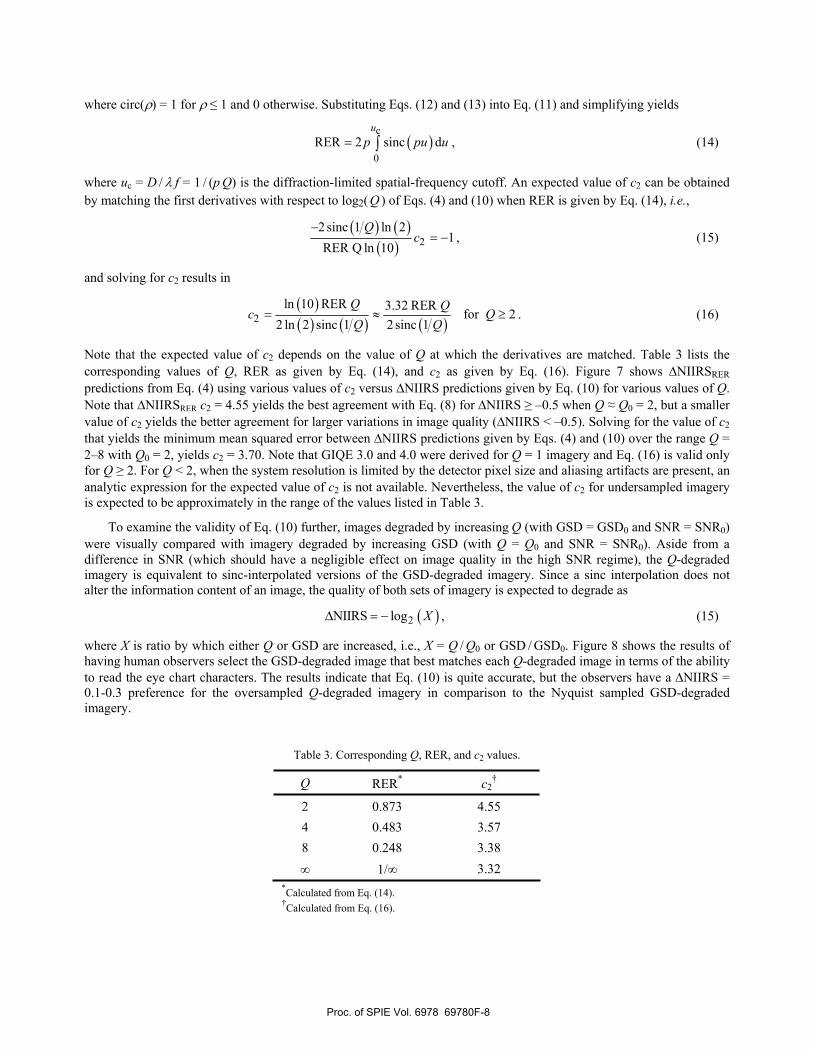
Note that the expected value of c2 depends on the value of Q at which the derivatives are matched. Table 3 lists the corresponding values of Q, RER as given by Eq. (14), and c2 as given by Eq. (16). Figure 7 shows NIIRSRERpredictions from Eq. (4) using various values of c2 versus NIIRS predictions given by Eq. (10) for various values of Q.Note that NIIRSRER c2 = 4.55 yields the best agreement with Eq. (8) for NIIRS –0.5 when Q Q0 = 2, but a smaller value of c2 yields the better agreement for larger variations in image quality ( NIIRS < –0.5). Solving for the value of c2that yields the minimum mean squared error between NIIRS predictions given by Eqs. (4) and (10) over the range Q = 2–8 with Q0 = 2, yields c2 = 3.70. Note that GIQE 3.0 and 4.0 were derived for Q = 1 imagery and Eq. (16) is valid only for Q 2. For Q < 2, when the system resolution is limited by the detector pixel size and aliasing artifacts are present, an analytic expression for the expected value of c2 is not available. Nevertheless, the value of c2 for undersampled imagery is expected to be approximately in the range of the values listed in Table 3.

To examine the validity of Eq. (10) further, images degraded by increasing Q (with GSD = GSD0 and SNR = SNR0)were visually compared with imagery degraded by increasing GSD (with Q = Q0 and SNR = SNR0). Aside from a difference in SNR (which should have a negligible effect on image quality in the high SNR regime), the Q-degraded imagery is equivalent to sinc-interpolated versions of the GSD-degraded imagery. Since a sinc interpolation does not alter the information content of an image, the quality of both sets of imagery is expected to degrade as

2NIIRS log X , (15)

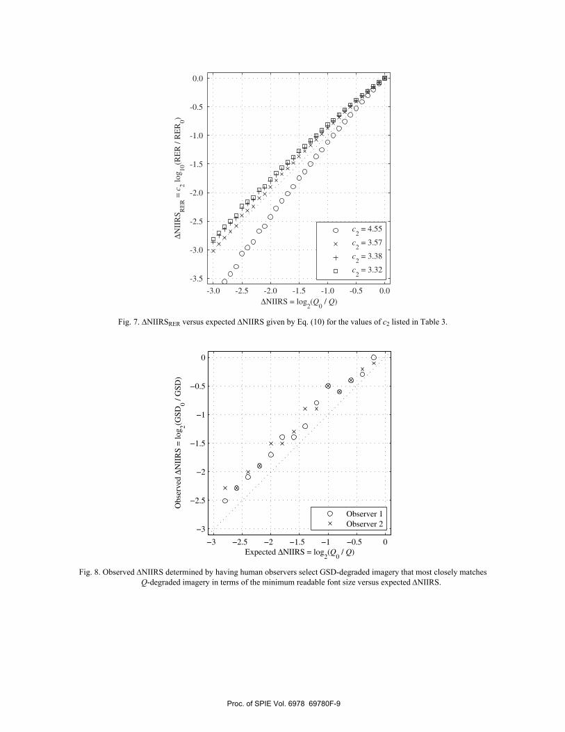
where X is ratio by which either Q or GSD are increased, i.e., X = Q / Q0 or GSD / GSD0. Figure 8 shows the results of having human observers select the GSD-degraded image that best matches each Q-degraded image in terms of the ability to read the eye chart characters. The results indicate that Eq. (10) is quite accurate, but the observers have a NIIRS = 0.1-0.3 preference for the oversampled Q-degraded imagery in comparison to the Nyquist sampled GSD-degraded imagery.

Table 3. Corresponding Q, RER, and c2 values.

Q RER* c2†

2 0.873 4.55 4 0.483 3.57 8 0.248 3.38

1/ 3.32 *Calculated from Eq. (14). †Calculated from Eq. (16).


∆NIIRS = log2(Q

0 / Q)

∆N

IIR

S RE

R =

c2 lo

g 10(R

ER

/ R

ER

0)

c2 = 4.55

c2 = 3.57

c2 = 3.38

c2 = 3.32

-3.0 -2.5 -2.0 -1.5 -1.0 -0.5 0.0

-3.0

-2.5

-2.0

-1.5

-1.0

-0.5

0.0

-3.5

Fig. 7. NIIRSRER versus expected NIIRS given by Eq. (10) for the values of c2 listed in Table 3.

3 2.5 2 1.5 1 0.5 0

3

2.5

2

1.5

1

0.5

0

Expected NIIRS = log2(Q

0 / Q)

Obs

erve

dN

IIR

S =

log 2(G

SD0 /

GSD

)

Observer 1Observer 2

Fig. 8. Observed NIIRS determined by having human observers select GSD-degraded imagery that most closely matches Q-degraded imagery in terms of the minimum readable font size versus expected NIIRS.


Observed ∆NIIRS = log2(GSD

0 / GSD)

Pred

icte

d∆

NII

RS

GIQE4.0

∆NIIRSGSD

∆NIIRSRER

∆NIIRSH

∆NIIRSG/SNR


0 / GSD)

Pred

icte

d∆

NII

RS

GIQE3.0

∆NIIRSGSD

∆NIIRSRER

∆NIIRSH

∆NIIRSG/SNR

(a) (b)

-3.0 -2.5 -2.0 -1.5 -1.0 -0.5 0.0

-2.5

-2.0

-1.5

-1.0

-0.5

0.0

0.5

-3.0

-3.0 -2.5 -2.0 -1.5 -1.0 -0.5 0.0

-2.5

-2.0

-1.5

-1.0

-0.5

0.0

0.5

-3.0

Fig. 9. GIQE (a) 3.0 and (b) 4.0 NIIRS predictions for imagery degraded by increasing Q with GSD = GSD0 and SNR = SNR0 versus the observed change in image quality determined by having observers select the GSD-degraded imagery that most closely matches each Q-degraded image in terms of image quality.

Figure 9 shows the GIQE NIIRS predictions for the Q-degraded image sequence versus the observed NIIRS, which resulted from having human observers selecting GSD-degraded imagery that matches each Q-degraded image in terms of image quality. The NIIRSRER predictions for both GIQE 3.0 with c2 = 3.32 and GIQE 4.0 with c2 = 2.817 are in excellent agreement with the observed NIIRS values, with coefficients of determination of R2 = 0.96 and 0.95, respectively. The values of c2 for GIQE 3.0 and 4.0 are a bit lower than the expected value of c2 = 3.70, which yields the minimum mean square error between NIIRS predictions given by Eqs. (4) and (8) over the range Q = 2–8 with Q0 = 2. Presumably, this is due to the above mentioned visual preference for oversampled imagery compared to Nyquist sampled imagery.

4.3 Signal-to-noise ratio

The dominant effect of noise (when properly accounted for by the Wiener filter) is to reduce the net image resolution. Figure 10 shows NIIRS predictions from GIQE 3.0 and 4.0 for SNR-degraded imagery (changing SNR with fixed GSD = GSD0 and Q = Q0) versus observed NIIRS, where the observed NIIRS were obtained by having human observers choose GSD-degraded imagery that most closely matches the quality of each SNR-degraded image. Figure 10 shows that

NIIRSRER is the dominant term affecting image quality even at very low SNRs, and that NIIRSRER alone is a fair indicator of the overall image quality. The coefficients of determination, R2, of the NIIRS predictions, based on the RER, G/SNR, and H terms of GIQE 3.0 and GIQE 4.0, for the SNR-degraded imagery are listed in Table 4.

Additionally, the presence of noise in an image has a masking effect, making it more difficult for an observer to perceive the true object features in an image. The influence of noise in this regard is not just dependent on the noise amplitude, but also depends on the spatial correlation (or equivalently the power spectrum) of the noise [13-15] resulting from post processing. In the GIQE, SNR is the measure of the noise amplitude in the raw imagery, G is the factor by



0 / GSD)

Pred

icte

d∆

NII

RS

GIQE4.0

∆NIIRSGSD

∆NIIRSRER

∆NIIRSH

∆NIIRSG/SNR


0 / GSD)

Pred

icte

d∆

NII

RS

GIQE3.0

∆NIIRSGSD

∆NIIRSRER

∆NIIRSH

∆NIIRSG/SNR

(a) (b)

-3.0 -2.5 -2.0 -1.5 -1.0 -0.5 0.0

-2.5

-2.0

-1.5

-1.0

-0.5

0.0

0.5

-3.0

-3.0 -2.5 -2.0 -1.5 -1.0 -0.5 0.0

-2.5

-2.0

-1.5

-1.0

-0.5

0.0

0.5

-3.0

Fig. 10. GIQE (a) 3.0 and (b) 4.0 NIIRS predictions for imagery degraded by decreasing SNR with GSD = GSD0 and Q = Q0. The GIQE predictions are plotted versus the observed change in image quality as determined by human observers

asked to choose a GSD-degraded image that most closely matches each SNR-degraded image.

Table 4. Coefficients of determination (R2) of NIIRS predictions for SNR-degraded imagery.

Image Quality Predictor GIQE 3.0* GIQE 4.0†

NIIRSRER 0.94 0.87

NIIRSRER + NIIRSG/SNR 0.92 0.89

NIIRSRER + NIIRSG/SNR + NIIRSH 0.90 0.86 *Corresponding to the data shown in Fig. 10(a). †Corresponding to the data shown in Fig. 10(b)

which the noise amplitude increases through post processing, and the coefficient c3 is presumably a measure of the net impact of the masking effect for noise with power spectra representative of those contained in the GIQE regression analysis. The impact of the masking effect on target detection can be predicted using various models of the human visual system [13,16]. Relating these methods to NIIRS predictions is beyond the scope of this paper.

The details of the post-processed noise power spectra are determined by the specifics of the optical system and the particular algorithm used for post processing. The details of the post processing used on the imagery for the GIQE 3.0 and 4.0 regression analyses were not published. Presumably the imagery was sharpened using a high-pass 3×3 or 5×5 sharpening kernel [17] as opposed to the Wiener filter we used. Additionally, there is evidence that much of the imagery used for the derivation of GIQE 4.0 was significantly oversharpened, compared to a Wiener reconstruction (see Section 4.4). Thus, it is difficult to assess the validity of the GIQE 3.0 or 4.0 coefficients for the G / SNR term in various scenarios.

4.4 Edge overshoot

The edge overshoot term is included in the GIQE to act as a penalty for edge ringing artifacts in oversharpened imagery. Here, we employ the following generalized definition of H for Q > 1


d ERER 1.25 when 0 for all , 3

H dmax ER ,| , 3 otherwise

xQ p x Q p Q p

xx x Q p Q p

, (18)

which simplifies to the definition of H given in Refs. [1,2] for Q = 1. Using the ideal net system transfer function Snet(u,v) given in Eq. (13) (which results from a Wiener filter in the high SNR regime with Q 2), the edge response is given by

ER 2 sinc 2 d

2 sinc 2 d ,

c c

xc c

x u u x U x x x

u u x x

(19)

where U(x) is the Heaviside step function. In this scenario, the maximum of ER(x) within the interval x [Q p, 3Q p]occurs at x = 3 / (2 uc) = 3Q p /2, which yields H = 1.03. This value of H is representative of edge ringing associated with the Gibbs phenomenon. Table 2 indicates that the edge overshoot factors used in the derivation of GIQE 4.0 were in the range H [0.9, 1.9] and had a mean value of 1.31. These large values of H (> 1.03) are evidence that the imagery was significantly oversharpened in comparison to analogous Wiener filter reconstructions. For all of the imagery considered in this paper, H [0.68, 1.06].

Out of all our simulated imagery, the NIIRSH predictions were non-negligible only for the SNR-degraded imagery. The binary definition of H in Eq. (18) leads to a discontinuity in NIIRSH that is visible in Figs. 10(a) and 10(b). The discontinuity occurs at low SNRs, for which the edge response after Wiener filtering becomes monotonic on x [Q p,3Qp]. We believe this is an artifact of the definition of H, since there is no physical basis for such a discontinuity.

While inclusion of an edge overshoot term as a penalty against edge ringing, even ringing due to the Gibbs phenomena, seems appropriate, it is difficult to determine the appropriate value of the GIQE coefficient c4 given the small range of H values used in this study. Table 4 indicates that NIIRSH degrades the coefficient of determination for the GIQE 3.0 and 4.0 predictions.

5. SUMMARYWe have examined the physical basis for the various terms in the GIQE and compared visual image quality assessments with GIQE predictions in an effort to determine the proper coefficients for use with Wiener filtered imagery from aberration-free, circular-aperture systems. Physical arguments and visual evaluation results indicate that the GIQE 3.0 coefficients c1 = –3.32 and c2 = 3.32 should be used for the log10(GSD) and log10(RER) spatial resolution terms, respectively, in order to preserve the notion that each factor of two in resolution is equivalent to one unit on the NIIRS. While it is more difficult to perceive the true features of an object when the noise in an image increases, the primary effect of noise (when properly accounted for in a Wiener filter) is to reduce the effective resolution of an imaging system. Results indicate that this loss in resolution due to noise is properly accounted for by the RER term when proper Wiener filtering is performed. While the edge overshoot term H was discussed, it is difficult to determine an appropriate value of c4 from this study due to the limited range of H values. Inclusion of NIIRSH using the GIQE 3.0 coefficient c4= –1.48 was found to degrade the image quality predictions. This is likely due to a discontinuity in NIIRSH associated with the binary-rule definition of H.

This work was funded by the U. S. Department of Defense.


REFERENCES

1. J. C. Leachtenauer and R. G. Driggers, Surveillance and Reconnaissance Imaging Systems, (Artech House, Boston, 2001).

2. J. C. Leachtenauer, W. Malila, J. Irvine, L. Colburn, and N. Salvaggio, “General Image-Quality Equation: GIQE,” Appl. Opt. 36, 8322-8328 (1997).

3. R. D. Fiete and T. Tantalo, “Image quality of increased along-scan sampling for remote sensing systems,” Opt. Eng. 38, 815-820 (1999).

4. R. D. Fiete, “Image quality and FN / p for remote sensing systems,” Opt. Eng. 38, 1229-1240 (1999). 5. R. D. Fiete and T. Tantalo, “Comparison of SNR image quality metrics for remote sensing systems,” Opt. Eng. 40,

574-585 (2001). 6. R. D. Fiete, T. A. Tantalo, J. R. Calus, and J. A. Mooney, “Image quality of sparse-aperture designs for remote

sensing,” Opt. Eng. 41, 1957-1969 (2002). 7. N. Wiener, Extrapolation, Interpolation and Smoothing of Stationary Time Series, (John Wiley & Sons, New York,

1950). 8. H. W. Bode and C. E. Shannon, “A simplified derivation of linear least square smoothing and prediction theory,”

Proc. IRE 38, 417-425 (1950). 9. C. W. Helstrom, “Image reconstruction by the method of least squares,” J. Opt. Soc. Am. 57, 297-303 (1967). 10. J. R. Fienup, D. Griffith, L. Harrington, A. M. Kowalczyk, J. J. Miller, and J. A. Mooney, “Comparison of

Reconstruction Algorithms for Images from Sparse-Aperture Systems,” Proc. SPIE 4792, 1-8 (2002). 11. D. J. Tolhurst, Y. Tadmor, and T. Chao, “Amplitude spectra of natural images,” Opthal. Physiol. Opt. 12, 229-232

(1992). 12. A van der Schaaf and J. H. van Hateren, “Modelling the power spectra of natural images: statistics and

information,” Vision Res. 36, 2759-2770 (1996). 13. P. F. Judy and R. G. Swennsson, “Lesion detection and signal-to-noise ratio in CT images,” Med. Phys. 8, 13-23

(1981). 14. P. A. Guignard, “A comparative method based on ROC analysis for the quantitation of observer performance in

scintigraphy,” Phys. Med. Biol. 27, 1163-1176 (1982). 15. K. J. Myers, H. H. Barrett, M. C. Borgstrom, D. D. Patton, and G. W. Seeley, “Effect of noise correlation on

detectability of disk signals in medical imaging,” J. Opt. Soc. Am. A, 2, 1752-1759 (1985). 16. K. J. Myers and H. H. Barrett, “Addition of a channel mechanism to the ideal-observer model,” J. Opt. Soc. Am. A

4, 2447-2457 (1987). 17. A. K. Jain, Fundamentals of Digital Image Processing, (Prentice-Hall, Englewood Cliffs, 1989).


analysis of the general image quality equation - the institute of optics

Documents