analysis of the potential for flow-induced deflection …
TRANSCRIPT

ANALYSIS OF THE POTENTIAL FOR FLOW-INDUCED DEFLECTION OF
NUCLEAR REACTOR FUEL PLATES UNDER HIGH VELOCITY FLOWS
A Thesis presented to the Faculty of the Graduate School
University of Missouri
In Partial Fulfilment
Of the Requirements for the Degree
Master of Science
by
CASEY JOHN JESSE
Dr. Gary L. Solbrekken, Thesis Supervisor
MAY 2015

The undersigned, appointed by the Dean of the Graduate School, have examined the
thesis entitled
ANALYSIS OF THE POTENTIAL FOR FLOW-INDUCED DEFLECTION OF
NUCLEAR REACTOR FUEL PLATES UNDER HIGH VELOCITY FLOWS
presented by Casey J. Jesse,
a candidate for the degree Master of Science,
and hereby certify that, in their opinion, it is worthy of acceptance.
Dr. Gary L. Solbrekken
Dr. Chung-Lung Chen
Dr. Hani Salim

ii
ACKNOWLEDGEMENTS
First and foremost, I would like to acknowledge my advisor, Dr. Gary
Solbrekken, for giving me the opportunity to work on this project. His guidance has been
invaluable in the completion of the research in this thesis. However, most importantly, he
has taught me to be the researcher I am today.
My fellow colleague, John Kennedy, also deserves thanks for working alongside
me on this project. The countless hours in the lab working through my questions as well
as discussing numerous theories has allowed the research in this thesis to be possible. I
must also thank Srisharan Govindarajan, Phillip Makarewicz, Abu Rafi Mohammad Iasir,
Annemarie Hoyer, Robert Slater, Alex Moreland, Robert Humphry, and Gerhard
Schnieders for helping make the lab an enjoyable environment to work in.
I would also like to thank the National Nuclear Security Administration (NNSA)
and Argonne National Laboratory (ANL) for supporting this research. Specifically, I
would like to thank Adrian Tentner, Erik Wilson, Earl Feldman, and John Stevens at
ANL.
Finally, I would like to thank my family, especially my parents for their support
throughout my life. My father and both my grandfathers provoked my interest in science
and engineering from a young age and I would not be the engineer I am today without
their inspiration. My mother has also been a constant inspiration while also always
reminding me to stay positive. Last, but certainly not least, I must acknowledge my
brother for being there through the times that I have found most difficult.

iii
TABLE OF CONTENTS
Acknowledgements ........................................................................................................ ii
List of Figures ............................................................................................................... vi
List of Tables...................................................................................................................x
Nomenclature ................................................................................................................ xi
Abstract ....................................................................................................................... xiii
Chapter 1 - Introduction..............................................................................................1
1.1 Pioneers of Nuclear Engineering........................................................................1
1.1.1 Atoms for Peace .........................................................................................3
1.1.2 Reduced Enrichment for Research and Test Reactors (RERTR) .................4
1.1.3 Research Reactors ......................................................................................6
1.2 University of Missouri Research Reactor (MURR) ............................................7
1.2.1 Previous and Current HEU Fuel Design......................................................9
1.2.2 Proposed LEU Fuel Design ...................................................................... 10
1.3 Purpose of Study ............................................................................................. 13
Chapter 2 - Interactions of Fluids and Structures....................................................... 17
2.1 Analytic Modeling of Hydro-Mechanical Stability........................................... 17
2.2 Experiments of Hydro-Mechanical Stability .................................................... 21
2.3 Numerical Techniques ..................................................................................... 25
Chapter 3 - Modeling of Fluid Flow around Fuel Plates ............................................ 32
3.1 Fluid Geometry ............................................................................................... 32
3.2 Analytic Fluid Model....................................................................................... 34
3.2.1 Frictional and Minor Losses ..................................................................... 35
3.2.2 Case of Unequal Flow Channels ............................................................... 37
3.3 Numeric Fluid Model ...................................................................................... 40
3.3.1 Geometry, Boundary Conditions, and Stopping Criteria ........................... 41
3.3.2 Fluid Mesh ............................................................................................... 42
3.3.3 Physics Models......................................................................................... 46
3.3.4 Turbulence Modeling Wall Treatments ..................................................... 47
3.4 Results of Preliminary Fluid Model Studies ..................................................... 51
3.4.1 Turbulence Model Study Results .............................................................. 51
3.4.2 Mesh Independence Study Results ............................................................ 55
3.4.3 High Density Mesh Results ...................................................................... 57

iv
Chapter 4 - Modeling the Deformation of a Fuel Plate .............................................. 60
4.1 Structure Geometry ......................................................................................... 60
4.2 Analytic Model ................................................................................................ 61
4.3 Numeric Model ............................................................................................... 62
4.3.1 Solid (Continuum) Elements..................................................................... 63
4.3.2 Mesh Studies ............................................................................................ 64
4.4 Results of Preliminary Solid Model Studies ..................................................... 65
4.4.1 Parametric Mesh Studies .......................................................................... 65
4.4.2 Formal Mesh Independence Study ............................................................ 67
4.4.3 Comparison to Analytic Model ................................................................. 68
Chapter 5 - Code Coupling Process .......................................................................... 70
5.1 Numeric Schemes ............................................................................................ 70
5.2 Numeric Code Coupling .................................................................................. 72
5.2.1 Loose (Explicit) Coupling ........................................................................ 72
5.2.2 Strong (Semi-implicit) coupling ............................................................... 76
5.2.3 Coupling Goals and Previous Stability Techniques ................................... 76
5.3 Empirical Stability Studies .............................................................................. 78
5.3.1 Flow Velocity and Temporal Step Size ..................................................... 78
5.3.2 Slenderness and Mass Density Ratios ....................................................... 79
5.3.3 The Courant Number and a Stability Parameter ........................................ 83
Chapter 6 - Code Coupling Results ........................................................................... 85
6.1 Time Step Study Results .................................................................................. 85
6.1.1 Initial Velocity Sweep Results .................................................................. 85
6.1.2 Second Velocity Sweep Results ................................................................ 91
6.2 Results of Slenderness and Mass Density Ratio Studies ................................. 100
6.2.1 Slenderness Ratio Results ....................................................................... 100
6.2.2 Mass Density Ratio Study Results .......................................................... 105
6.3 Discussion of a Stability Parameter ................................................................ 107
Chapter 7 - Experiment Setup and Comparison to FSI Models ................................ 111
7.1 Experimental Setup (University of Missouri Flow Loop) ............................... 111
7.1.1 Flat Plate Test Section ............................................................................ 113
7.1.2 Previous Laser Positioning Systems and Channel Mapping Procedure .... 114
7.1.3 Flow Experiment Procedure ................................................................... 116
7.2 Experiment Results and Comparison to FSI Models ...................................... 117

v
7.2.1 Channel Mapping Results ....................................................................... 117
7.2.2 Flow Experiment Results and Comparison to Models ............................. 121
7.3 Laser Positioning System............................................................................... 129
7.3.1 New Positioning System Design ............................................................. 129
7.3.2 Manufacturing Processes for Custom Parts ............................................. 132
7.3.3 Additive Manufacturing using FDM ....................................................... 135
Chapter 8 – Modeling of MURR-Specific Fuel Plates ............................................. 142
8.1 Curved Plate Modeling .................................................................................. 142
8.2 Curved Plate Results ...................................................................................... 144
8.2.1 Case 1 Results ........................................................................................ 144
8.2.2 Case 2 Results ........................................................................................ 146
8.3 Comparing Flat and Curved Plates ................................................................. 149
Chapter 9 - Closure................................................................................................. 150
9.1 Conclusions ................................................................................................... 150
9.2 Future Work .................................................................................................. 151
Appendix 1 – Model Benchmarking: The ‘Snap’ Velocities ......................................... 153
Appendix 2 – ANL Memo: Flow Velocity through MURR .......................................... 155
Appendix 3 – MATLAB Code for Analytic Flow Model ............................................. 156
Appendix 4 – MATLAB Code for Analytic Plate Model ............................................. 161
References ................................................................................................................... 162

vi
LIST OF FIGURES
Figure 1-1. Replica of Meitner, Hahn, and Strassmann’s setup for irradiating uranium [1].
........................................................................................................................................1 Figure 1-2. Artist’s depiction of Chicago Pile 1 at the University of Chicago [1]. ............3
Figure 1-3. Overhead photo of the MURR pool and core assembly. .................................7 Figure 1-4. (A) 3D view of the reactor core assembly and (B) 2D vertical cross-section
[12]..................................................................................................................................8 Figure 1-5. Reactor core assembly 2D horizontal cross section [12]. ................................9
Figure 1-6. Cross section of UAlx HEU fuel plate currently used in the MURR’s core. .. 10 Figure 1-7. (A) Photo and (B) 3D drawing of a mock MURR fuel element [12]. ............ 10
Figure 1-8. Cross section of U-10Mo LEU fuel plate proposed for use in the MURR’s
core. .............................................................................................................................. 11
Figure 2-1. Three-field system of an aeroelastic problem [33]. ....................................... 27 Figure 3-1. Fluid model geometry (not to scale). ............................................................ 32
Figure 3-2. Minor and major losses through the flow geometry. ..................................... 34 Figure 3-3. Parameters for computing contraction and expansion losses. ....................... 35
Figure 3-4. 1D analytic model’s axial pressure profile solution at 8 m/s. ........................ 40 Figure 3-5. Fluid geometry in Star-CCM+. .................................................................... 41
Figure 3-6. Fluid geometry in Abaqus both un-partitioned and partitioned. .................... 44 Figure 3-7. Imported mesh in Star-CCM+. ..................................................................... 45
Figure 3-8. Fluid mesh in Star-CCM+ with parameters for the mesh independence study.
...................................................................................................................................... 46
Figure 3-9. Law of the wall and log law showing the regions of the velocity profile near
the wall. ......................................................................................................................... 49
Figure 3-10. Comparing near wall meshes of high y+ and low y+ wall treatments, red line
signifies the velocity profile near the wall and the yellow point is the near wall cell
centroid. ........................................................................................................................ 50
Figure 3-11. Axial pressure profiles for the k-ε models overlaid on the analytic model’s
solution.......................................................................................................................... 54
Figure 3-12. Axial pressure profiles for the k-ω models overlaid on the analytic model’s
solution.......................................................................................................................... 55
Figure 3-13. Results of how the inlet pressure varied from mesh to mesh with % error
from the analytic model included. .................................................................................. 56
Figure 3-14. Results of how the average surface pressure on the plate varied from mesh to
mesh with % difference from the previous mesh included. ............................................. 57
Figure 3-15. High density (~14 million cells) mesh and Mesh 5 at the leading edge of the
plate. ............................................................................................................................. 58
Figure 3-16. Axial pressure profiles with the high-density mesh and Mesh 5 with zoom of
the leading edge. ............................................................................................................ 59
Figure 4-1. Aluminum 6061-T6 flat plate....................................................................... 60 Figure 4-2. Geometry and boundary conditions of a simple flat beam (Y is into the page).
...................................................................................................................................... 61 Figure 4-3. Flat plate geometry in Abaqus. .................................................................... 63
Figure 4-4. Solid continuum element mesh in Abaqus.................................................... 64 Figure 4-5. Results of element variance along the plate length. ...................................... 66

vii
Figure 4-6. Results of element variance along the plate width. ....................................... 66 Figure 4-7. Results of element variance through the plate thickness. .............................. 67
Figure 4-8. Results of mesh independence study in Abaqus. .......................................... 68 Figure 4-9. Comparison of the Abaqus model with the simple analytic model. ............... 69
Figure 5-1. Grid used in the finite difference derivations of Eqs. (5.2)-(5.3). .................. 71 Figure 5-2. Loose (explicit) coupling using a sequentially staggered approach. .............. 73
Figure 5-3. Abaqus and Star-CCM+ explicit coupling process. ...................................... 74 Figure 5-4. Converged pressure and deflection distributions on the fluid/structure
interface......................................................................................................................... 75 Figure 5-5. Trends for how the avg. ch. velocity varies as the pressure drop increases for
various fluid densities, trends were used to fix the momentum for the density ratio study.
...................................................................................................................................... 82
Figure 6-1. Evolution of plate deflection at “Point C” from 3 to 6 m/s, solid line = 0.5 s
time step and dotted line = 0.1 s time step, zoom-in shows convergence behavior at low
velocities. ...................................................................................................................... 86 Figure 6-2. Evolution of plate deflection at “Point C” from 6.5 to 7.5 m/s, solid line =
0.05 s time step and dotted line = 0.0375 s time step. ..................................................... 87 Figure 6-3. Evolution of plate deflection at “Point C” at 7.75 and 8 m/s, solid line =
0.0325 s time step and dotted line = 0.03125 s time step, zoom-in shows early chaotic
behavior......................................................................................................................... 87
Figure 6-4. Maximum deflection at the leading edge of the plate vs. avg. ch. velocity. ... 89 Figure 6-5. Contours of deflection at 5 and 8 m/s, flow moves down in the –y direction.
...................................................................................................................................... 90 Figure 6-6. Deflection profile extracted from the axial centerline of the plate in Abaqus.
...................................................................................................................................... 90 Figure 6-7. Evolution of plate deflection at “Point C” at 2 m/s with different time step
sizes with zoom of stability with time steps of 0.5 and 2 s. ............................................. 91 Figure 6-8. Evolution of plate deflection at “Point C” at 5 m/s with different time step
sizes with zoom of stability with time steps at 0.075, 0.5, and 2 s. ................................. 92 Figure 6-9. Response of a structurally deforming lid-driven cavity by Forester et al.
showing how decreasing the time step beyond a certain threshold causes instability [36].
...................................................................................................................................... 94
Figure 6-10. Map of stable, mildly unstable, and unstable time steps from 4.75 to 8.25
m/s. ............................................................................................................................... 95
Figure 6-11. Evolution of plate deflection at “Point C” with various time steps at 6.5 m/s.
...................................................................................................................................... 96
Figure 6-12. Non-linear behavior of Star-CCM+’s built-in mesh morpher, contour is of
cell volume, both meshes are from 6.5 m/s models, A has ∆t = 5s and B has ∆t = 0.03s. ...................................................................................................................................... 97 Figure 6-13. Map of the Courant number for models completed in the second velocity
sweep. ........................................................................................................................... 99 Figure 6-14. Evolution of plate deflection at “Point C” with various plate lengths at 6
m/s with zoom-in of the stable plate lengths................................................................. 101 Figure 6-15. Axial plate deflection (blue curves) and differential pressure (red curves) on
the plate for each plate length at 6 m/s. ........................................................................ 102

viii
Figure 6-16. Differential pressure on the plate at 6 m/s, plate deformation was not
allowed (the plate was held rigid). ............................................................................... 103
Figure 6-17. Evolution of plate deflection at “Point C” with various plate lengths at 7
m/s. ............................................................................................................................. 104
Figure 6-18. Axial plate deflection (blue curves) and differential pressure (red curves) on
the plate at 7 m/s. ......................................................................................................... 104
Figure 6-19. Evolution of plate deflection at “Point C” with various fluid densities. ... 106 Figure 6-20. Map of Cs as velocity and plate length vary with FSI model results overlaid.
.................................................................................................................................... 108 Figure 6-21. Map of Cs as velocity and fluid density vary with FSI model results
overlaid. ...................................................................................................................... 109 Figure 7-1. University of Missouri Hydro-Mechanical Flow Loop. .............................. 112
Figure 7-2. System flow rate calibration curve. Note: System is in (+) pressure mode. . 112 Figure 7-3. Flat plate test section diagram and photo. .................................................. 113
Figure 7-4. Laser positioning system for channel mapping (left photo) and flow
experiments (right photo) [49]. .................................................................................... 115
Figure 7-5. Measurement locations for fluid channel mapping [49]. ............................. 116 Figure 7-6. Measurements for all nine sweeps through the 120 location measurement
process. ....................................................................................................................... 118 Figure 7-7. Standard deviation of the nine trials at each measurement location. ........... 119
Figure 7-8. Average of the nine trials at each measurement location for both channels as
well as the difference between Channel 1 and Channel 2 [49]. ..................................... 120
Figure 7-9. Large and small channel gap thicknesses and channel difference at
approximately the centerline of the plate. ..................................................................... 120
Figure 7-10. Comparison of the experiment with the models showing the change in
channel gap thickness, points connected with dashed lines are experimental data and solid
lines are solutions from the models. ............................................................................. 121 Figure 7-11. Comparison of the model (solid line) to the experiment (dashed lines) at
~2.06 m/s. .................................................................................................................... 122 Figure 7-12. Comparison of the model (solid lines) to the experiment (dashed lines) at
~2.77 m/s. .................................................................................................................... 123 Figure 7-13. Comparison of the model (solid lines) to the experiment (dashed lines) at
~3.46 m/s. .................................................................................................................... 123 Figure 7-14. Comparison of the model (solid lines) to the experiment (dashed lines) at
~4.55 m/s. .................................................................................................................... 124 Figure 7-15. Comparison of the model (solid line) to the experiment (dashed lines) at
~5.14 m/s. .................................................................................................................... 124 Figure 7-16. Comparison of the model (solid lines) to the experiment (dashed lines) at
~6.8 m/s....................................................................................................................... 125 Figure 7-17. Comparison of the model (solid lines) to the experiment (dashed lines) at
~7.75 m/s. .................................................................................................................... 125 Figure 7-18. Comparison of the channel difference assumed in the models, measured
during the channel mapping, and measured just before the flow experiments. .............. 127 Figure 7-19. Full rendering of the new laser positioning system. .................................. 131
Figure 7-20. Detailed view of the horizontal rail. ......................................................... 131 Figure 7-21. Simplified beam analysis for the lead screw bearing mount. .................... 135

ix
Figure 7-22. Tool path for a single layer of a rectangular block. ................................... 136 Figure 7-23. Process of fused deposition modeling (FDM). ......................................... 137
Figure 7-24. Kossel delta printer, which utilizes the FDM process. .............................. 138 Figure 7-25. Example of a honeycomb infill that requires rapid changes in direction of
the extruder. ................................................................................................................ 139 Figure 7-26. Imported STL file, sliced rendering, and printed part with cut showing
honeycomb infill. Part shown is the stepper motor mount for the axial movement........ 139 Figure 7-27. Fully assembled laser positioning system. ................................................ 140
Figure 8-1. Top view of the MURR core with photo of a mock fuel element [12]. ....... 142 Figure 8-2. Top view of the curved plate FSI model geometry (flow is into the page). . 143
Figure 8-3. Two distinct cases for curved plate modeling. ............................................ 143 Figure 8-4. Case 1 maximum deflection vs. average channel velocity. ......................... 145
Figure 8-5. Abaqus contour plots of radial deflection at 25 and 40 m/s with a 0.66 mm
plate. ........................................................................................................................... 145
Figure 8-6. Axial centerline deflection at 25 to 40 m/s with a 0.66 mm plate................ 146 Figure 8-7. Case 2 maximum deflection results vs. average channel velocity. .............. 147
Figure 8-8. Leading edge bending into both channels at 25 m/s with a 0.66 mm plate,
contour is showing radial deflection (Case 2). .............................................................. 147
Figure 8-9. Excessive radial deflection into the 2.54 mm channel at 30 m/s. ................ 148 Figure 8-10. Excessive radial deflection into the 2.54 mm channel at 30 m/s, deflection is
19.41 mm. ................................................................................................................... 148

x
LIST OF TABLES
Table 1-1. LEU fuel design parameters from 2009 Feasibility Analysis [12]. ................. 12
Table 1-2. LEU fuel design parameters after RC redesign [13]. ..................................... 13 Table 3-1. Geometric parameters for fluid models. ........................................................ 33
Table 3-2. Fluid properties for water. ............................................................................. 33 Table 3-3 Details of meshes in Star-CCM+ mesh independence study. .......................... 46
Table 3-4. Physics models used in Star-CCM+. ............................................................. 47 Table 3-5. RANS turbulence models explored. .............................................................. 47
Table 3-6. Wall y+ values of near wall cells on the channel walls and plate surface. ....... 52
Table 3-7. Pressure drop for each turbulence model with % difference from analytic
model. ........................................................................................................................... 53 Table 4-1. Al-6061-T6 material properties [43].............................................................. 61
Table 4-2. Details of the mesh study in Abaqus. ............................................................ 65 Table 4-3. Details of meshes in Abaqus mesh independence study. ................................ 65
Table 5-1 Density ratio, and average channel velocity results for fixed momentum
analysis.......................................................................................................................... 82
Table 6-1 Wall clock time for the FSI models to converge to a steady state. .................. 88 Table 7-1. Nominal dimensions of the test section assembly. ....................................... 114
Table 7-2. Axial laser locations during the experiment (distances are from the plate's
trailing edge) ............................................................................................................... 117
Table 7-3. Material cost for traditional manufacturing. ................................................ 132 Table 7-4. Material cost for additive manufacturing, cost per cm
3 is ~$0.05. ................ 133
Table 7-5. Material property comparison of Al 6061-T6 and polylactic Acid [43, 51]. . 133 Table 8-1. Comparing the maximum deflection with flat and curved plates. ................. 149

xi
NOMENCLATURE
General
a Structure thickness
b Channel 1 thickness
c Channel 2 thickness
d Structure width
f friction factor
g gravity
h Average channel thickness
k k loss coefficient
�̇� Mass flow rate
t time
y+ non-dimensional distance
from wall
A Area
Dh Hydraulic Diameter
E Elastic modulus
I Area moment of inertia
L Length
MA Added-mass effect operator
M Moment
P Pressure
Red Reynolds number
V Velocity
Greek
α One-half of plate arc
ε Wall roughness height
ρ Density
υ Poisson’s ratio
𝜏𝑤 Wall shear stress
μ Eigenvalue
Subscripts
c Miller critical velocity
ch channel
f fluid
s structure
Abbreviations
ANL Argonne National
Laboratory
ATR Advanced Test Reactor
CAD Computer Aided Drafting
CFD Computational Fluid
Dynamics
CFL Courant-Freidrichs-Lewy
FEA Finite Element Analysis
FDM Fused Deposition Modeling
FSI Fluid-Structure Interaction
GTRI Global Threat Reduction
Initiative
HEU High Enriched Uranium
HIFR High Flux Isotope Reactor
IAEA International Atomic
Energy Agency
INL Idaho National Laboratory
LEU Low Enriched Uranium
NNSA National Nuclear Security
Administration
MITR Massachusetts Institute of
Technology Reactor
MURR University of Missouri
Research Reactor
NBSR National Bureau of
Standards Reactor
NIST National Institute of
Standards and Technology

xii
ORNL Oak Ridge National
Laboratory
PDE Partial Differential Equation
PLA Polylactic Acid
RERTR Reduced Enrichment for
Research and Test Reactors
STL Stereolithography

xiii
ABSTRACT
The University of Missouri Research Reactor (MURR) is one of five High
Performance Research Reactors (HPRRs) in the U.S. that still utilizes high enriched
uranium (HEU) fuel. In accordance with the Department of Energy’s Global Threat
Reduction Initiative (GTRI), these remaining HPRRs must convert from weapons-usable
HEU fuel to proliferation-resistant low enriched uranium (LEU) fuel.
A novel monolithic LEU fuel with a U-10Mo fuel meat is under consideration to
replace the current U-Al dispersion HEU fuel. While the new LEU fuel design will
accomplish the GTRI mission, the in-reactor safety of these proposed LEU fuel plates
must be investigated. Questions have been raised about how the thinner laminate
sandwich structure of the LEU fuel plates will hydro-mechanically respond under the
high velocity coolant flows within the reactor cores. If the fuel plates deform such that
the flow of coolant is choked off the temperature of a fuel plate could increase enough to
cause it to rupture and potentially release fission gas into the coolant system.
The purpose of this research was to develop a set of numerical tools to access the
flow-induced deformation of the proposed LEU fuel by coupling the commercial
computational fluid dynamics (CFD) code, Star-CCM+, with the finite element analysis
(FEA) code, Abaqus to build fluid-structure interaction (FSI) models. These FSI models
are inherently unstable due to the nature of a high velocity incompressible flow
interacting with a slender fuel plate. The temporal discretization, slenderness ratio, and
mass density ratio greatly affect the stability of the FSI models, thus the temporal step
size was carefully controlled to promote stability.
The results of the FSI models were then benchmarked against experiments
conducted using a hydro-mechanical flow loop. A plan for future experiments and FSI

xiv
models is discussed to help facilitate convergence of the experimental data with the
model’s solution. A successful benchmarking will allow these numerical tools to be
utilized in complicated models for qualifying the safe-use of the proposed LEU fuel.

1
CHAPTER 1 - INTRODUCTION
1.1 Pioneers of Nuclear Engineering
In 1938, Lise Meitner, Otto Hahn and Fritz Strassmann performed
experimentation into the theory that splitting an atom of a heavy element, such as
uranium, would produce two smaller atoms of different elements. A replica of their
experimental setup, which irradiated a sample of uranium, is shown in Figure 1-1.
Unfortunately, Meitner’s Jewish ancestry forced her to flee Germany before their work
could be completed. Nonetheless, Hahn and Strassmann completed the tedious
experiment and shared its puzzling results with her [1].
With the help of her nephew, physicist Otto Frisch, she was able to interpret the
confusing data by hypothesizing and theoretically proving that the uranium nuclei were
splitting to form two lighter elements, namely barium and krypton, expel additional
neutrons, and release a large amount of energy. These latter two products account for the
loss in mass that occurs when the uranium nuclei split. Frisch suggested the process be
called “nuclear fission” after the similar fission process of biological cells. Hahn
eventually went on to win the Nobel Prize for Chemistry in 1944 for his discovery [1].
Figure 1-1. Replica of Meitner, Hahn, and Strassmann’s setup for irradiating uranium [1].

2
Following Hahn and Strassmann’s discovery and later interpretation as nuclear
fission by Meitner and Frisch, Enrico Fermi and Herbert Anderson corroborated their
results in the United States and experimentally demonstrated that indeed more neutrons
were expelled than absorbed by the uranium nuclei. Shortly after Fermi and Leo Szilard
designed a device that could theoretically allow a nuclear reaction to become self-
sustaining, i.e. a nuclear reactor [2].
Postulating that a self-sustaining nuclear reaction could be implemented in the
design of a weapon, Szilard, Eugene Wigner, and Edward Teller, drafted and sent the
famous letter signed by Albert Einstein, to President Franklin D. Roosevelt. The letter
stressed that Nazi Germany was likely developing an atomic bomb. This led Roosevelt to
develop the S-1 Uranium Committee, which ultimately led to the Manhattan Project [3].
To demonstrate a self-sustaining nuclear reaction was possible, Fermi and Arthur
Compton, head of the Metallurgical Laboratory at the University of Chicago (U.C.), built
a 56-layer lattice structure using 22,000 uranium slugs, which was comprised of 40 tons
of uranium oxide and 6 tons of uranium metal. An artist’s rendition of this structure,
known as Chicago Pile 1 (CP-1) is shown in Figure 1-2. The pile was built under the
stands of U.C.’s Stagg Field, which is rather shocking since the results of a self-
sustaining nuclear reaction were still unknown at the time. The key to CP-1’s self-
sustainment was the inclusion of graphite in the pile.
Fermi identified that lower energy neutrons, or ‘thermal’ neutrons, were more
likely to be absorbed by atoms. In order to decrease the energy of the neutrons expelled
during the fission process, they included 380 tons of graphite blocks in CP-1. The
graphite acted as a moderator, which slowed down the speed of the neutrons and

3
effectively increased the likelihood of them fissioning other uranium nuclei. On
December 2, 1942, CP-1 became the first self-sustaining nuclear reactor. The reactivity
was controlled with rods of cadmium, indium, and silver [2].
Figure 1-2. Artist’s depiction of Chicago Pile 1 at the University of Chicago [1].
After the self-sustainment of CP-1 the Manhattan Project went on to spend nearly
$2 billion dollars, employ more than 130,000 people, and ultimately drop two atomic
bombs on Japan during World War II. Namely, “Little Boy”, a uranium-235 (235
U) fueled
gun-type fission weapon, on Hiroshima on August 6, 1945 and “Fat Man”, an implosion-
type weapon with a plutonium core, on Nagasaki on August 9, 1945.
1.1.1 Atoms for Peace
Following the end of World War II, extensive testing of nuclear weapons was
conducted by the United States and Russia. These nuclear tests and the aftermath of
dropping “Little Boy” and “Fat Man” on Hiroshima and Nagasaki created a sense of fear
and uncertainty within the general public about the effects of nuclear technology. In
response, President Dwight D. Eisenhower spoke before the United Nations General

4
Assembly, which later became known as the “Atoms for Peace” speech on December 8,
1953. He pledged the United States was determined “…to help solve the fearful atomic
dilemma – to devote its entire heart and mind to find the way by which the miraculous
inventiveness of man shall not be dedicated to his death, but consecrated to his life” [4].
The speech provoked the creation of the Treaty on the Non-Proliferation of
Nuclear Weapons and launched many proliferation-resistant programs such as the
International Atomic Energy Agency (IAEA). The world made great progress in utilizing
nuclear technology to improve society rather than destroy it. This progress included, but
was not limited to, building hundreds of nuclear power plants and research reactors
around the world for energy production and peaceful nuclear research, producing
numerous medical isotopes for the millions of medical procedures completed each year,
and developing advanced materials [4].
Unfortunately, Atoms for Peace also provided a cover for the nuclear arms race
during the Cold War that extended through the 1960s and 70s. During Eisenhower’s time
in office, the nuclear arsenal increased more than twentyfold in the U.S. Furthermore,
under Atoms for Peace programs, the U.S. exported over 25 tons of highly enriched
uranium (HEU) to more than 30 countries and under similar programs, Russia exported
over 11 tons of HEU [5] [6]. Uranium is considered highly enriched when the 235
U
concentration is > 20%. These exports aided in creating 100 tons of civil HEU worldwide
causing major concern from both a proliferation and nuclear terrorism sense [7].
1.1.2 Reduced Enrichment for Research and Test Reactors (RERTR)
India’s first nuclear weapon test in 1974 and other unregulated nuclear activities
in several countries caused the U.S. to restructure their nonproliferation policy. Under the

5
Gerald Ford and Jimmy Carter administrations of the 1970s, the U.S. began searching for
ways to stifle proliferation threats such as the use of HEU in civilian applications. Thus in
1978, the Reduced Enrichment for Research and Test Reactors (RERTR) program was
initiated in order to develop “the technical means to utilize LEU instead of HEU in
research reactors without significant penalties in experiment performance, operating
costs, reactor modifications, and safety characteristics” [8]. Low enriched uranium or
LEU uranium that has a 235
U concentration of < 20%.
In 2004, the National Nuclear Security Administration’s (NNSA) Office of
Defense Nuclear Nonproliferation merged the RERTR program with various other HEU
minimization programs to form the Global Threat Reduction Initiative (GTRI). The new
mission was “… to, as quickly as possible, identify, secure, remove, and/or facilitate the
disposition of high risk vulnerable nuclear and radiological materials around the world
that pose a threat to the U.S. and the international community.” Specifically one part of
the GTRI’s mission, was to work “…,domestically and internationally, [in order to]
implement the long-standing U.S. policy to minimize and eliminate the use of highly
enriched uranium (HEU) in civilian applications by working to convert research and test
reactors and isotope production facilities to the use of low enriched uranium (LEU)” [9].
To fulfill the mission of converting research reactors to LEU, the GTRI has
converted 20 U.S. reactors to use currently licensed LEU fuel. However, five U.S.
research reactors, considered high-performance reactors, are still fueled with HEU. The
GTRI is currently developing a unique foil based LEU fuel since the reactors cannot
convert to the existing licensed LEU fuels while maintaining their performance standards.
6
The GTRI has also converted 47 reactors in 34 countries to LEU fuel, while also
verifying the shutdown of 20 HEU reactors in 11 countries [9].
1.1.3 Research Reactors
Research reactors were (and still are) seen as an essential step for many
developing countries to harness nuclear power. They also serve many other diverse needs
such as medical and industrial isotope production, neutron beam based research,
advanced materials research, and technology development for existing and advanced
nuclear power capabilities [1]. Research reactors require high power densities typically
achieved by utilizing unique reactor designs with HEU fuels. Hence, the U.S and
Russia’s large export of HEU during the latter half of the last century.
More than 670 research reactors were built and commissioned around the world
since CP-1 became self-sustaining. About 246 of these reactors are still in operation as of
2010. Currently, many research reactors are being refurbished to meet modern standards
since some are over 40 years old [10]. One of these aging reactors is the University of
Missouri Research Reactor (MURR). After beginning operation in 1966 at 5 MW, it was
upgraded to 10 MW in 1974. When the MURR was designed and constructed research
reactors utilized HEU fuel with 235
U enrichments of 90% or greater in order to achieve
the desired performance. However, a new LEU fuel that uses a uranium foil is currently
being investigated and developed under the GTRI as an alternative proliferation-resistant
fuel for MURR and 4 other U.S. high performance research reactors. These four other
domestic reactors include Advanced Test Reactor (ATR) at Idaho National Laboratory
(INL), the High Flux Isotope Reactor (HIFR) at Oak Ridge National Laboratory (ORNL),
the Massachusetts Institute of Technology Reactor (MITR), and the National Bureau of

7
Standards Reactor (NBSR) at the National Institute of Standards and Technology (NIST)
[11].
1.2 University of Missouri Research Reactor (MURR)
The MURR is a light water moderated and cooled pressurized open pool-type
research reactor located on the University of Missouri campus in Columbia, MO. The
maximum thermal power level is 10 MW under forced cooling and 50 kW under natural
convection. The core of the reactor is within a 3.05 m (10’) aluminum-lined pool that is
9.10 m (30’) deep. An overheard view of the reactor core assembly within its pool is
shown in Figure 1-3.
Figure 1-3. Overhead photo of the MURR pool and core assembly.
Four major regions create the reactor core assembly including the flux trap, the
fuel zone, the control blades, and the beryllium/graphite reflectors. These four regions of
the reactor core assembly are shown and labeled in Figure 1-4.

8
Figure 1-4. (A) 3D view of the reactor core assembly and (B) 2D vertical cross-section [12].
The first region of the assembly is the flux trap located within the inner pressure
vessel. It is the most reactive part of the core and therefore has its own cooling system
using water recirculated from the pool. The next region is the fuel zone, which is
pressurized to 80 psia within an annulus comprised of two cylindrical aluminum pressure
vessels. Within this pressurized annulus, there are eight identical fuel elements with 24
HEU fuel plates in each element. The control blade region contains five control blades
that regulate the fission rate of 235
U by absorbing neutrons to reduce reactivity. Four of
the blades are Boral and one is stainless steel. The control blade region is situated
between the outer pressure vessel of the fuel zone and the inner reflector wall. The final
region containing the reflectors has two main parts. The first part is the beryllium sleeve
that surrounds the control blades shown as the shaded annulus in Figure 1-5. The second
part contains twelve aluminum encased graphite wedges that form an annulus. These
graphite elements surround the beryllium portion of the reflector region and they are
labeled in blue in Figure 1-5.

9
Figure 1-5. Reactor core assembly 2D horizontal cross section [12].
1.2.1 Previous and Current HEU Fuel Design
Initially the MURR was started as a 5 MW facility in 1966 with a uranium-
aluminum (U-AL) alloy fuel. This fuel was loaded to a maximum of 650 grams of 235
U.
At the time, the U-Al fuel had been extensively tested in reactors throughout the world
including the Materials Test Reactor (MTR) and the Engineering Test Reactor (ETR) at
the Idaho National Engineering Laboratory, now the Idaho National Laboratory [12].
In 1971, to reduce the cost of the fuel and the amount of 235
U used per MWd of
energy produced, the MURR converted to a uranium-aluminide powder dispersion
(UAlx) fuel. The new UAlx fuel meat is pressed into a rigid structure with a 235
U
enrichment of 93%. The 610 mm (24”) length of fuel meat is then sandwiched by 0.38
mm (15 mils) of Al 6061-T6 cladding on the inner and outer radii as shown in Figure 1-6.
Regardless of the plate width the edges of each plate has 3.68 mm (145 mil) of unfueled
cladding. The finished UAlx fuel plate is 648 mm (25.5”) long [12].

10
Figure 1-6. Cross section of UAlx HEU fuel plate currently used in the MURR’s core.
Twenty-four of these fuel plates are then swaged concentrically into two 3.81 mm
(15 mils) thick Al-6061 side edges as shown by the photo of a mock MURR fuel element
in Figure 1-7. Each plate is separated by 2.032 mm (80 mils) to create channels for the
flowing light water to cool and moderate the fission reaction. To regulate this spacing and
to provide additional structural support, a comb is placed at the top and bottom of the fuel
plates. The elements are then held together with an end cap on both the top and bottom of
the element. Each element is loaded to a maximum of 775 grams of 235
U with a fuel
density of 1.53 grams/cm3. Eight of these 826 mm (32.5”) long fuel elements are
arranged into an annulus within the inner and outer pressure vessel walls numbered in
green in Figure 1-5 [12].
Figure 1-7. (A) Photo and (B) 3D drawing of a mock MURR fuel element [12].
1.2.2 Proposed LEU Fuel Design
While many research reactors around the world have converted to using LEU fuel
rather than weapons-usable HEU fuel, the MURR’s highly compact core design requires

11
a much higher loading density of 235
U than the currently qualified LEU fuels. A
feasibility analysis was completed on a new monolithic uranium fuel with 10%
molybdenum (U-10Mo) by MURR and the GTRI Reactor Conversion Program at
Argonne National Laboratory (ANL) in 2009 [12]. In the analysis, five major concerns in
conversion to LEU fuel were: (1) matching the performance capabilities of the current
HEU fuel element, (2) not increasing the MURR’s fuel storage requirements, (3) having
sufficient excess reactivity, (4) maintaining or enhancing neutron flux, and (5) most
importantly, preserving operation costs compared to the HEU core. The U-10Mo design
from the feasibility analysis met or exceeded all the aforementioned design concerns.
The general design of the U-10Mo LEU fuel is shown in Figure 1-8. The overall
design of the elements was kept the same to minimize changes to the existing core;
however, the overall structure of the fuel was different. The fuel’s meat was replaced
with a U-10Mo foil with a 235
U enrichment of 19.75%. A 0.025 mm (1 mil) layer of
zirconium surrounded the meat to form a barrier between the Al 6061-T6 cladding and
the U-10Mo meat. Both the meat and the cladding thicknesses were reduced in the LEU
design. These reductions decreased the overall plate thickness causing an increase in the
water-to-metal ratio within the core, otherwise; the necessary reactivity could not be
obtained with the reduced 235
U enrichment.
Figure 1-8. Cross section of U-10Mo LEU fuel plate proposed for use in the MURR’s core.

12
The thicknesses of the meat, cladding, coolant channels, and overall plate are
shown in Table 1-1 for the 24-plate 2009 design. Unfortunately, the Fuel Development
(FD) and Fuel Fabrication Capability (FFC) pillars of the GTRI’s RERTR program found
that some of the initial assumptions for the U-10Mo fuel plate design in 2009 needed
adjustments. For example, the 2009 design called for 0.25 mm (10 mils) of aluminum
clad to surround the LEU foil for plate 3 through 23 in each fuel element. The FD and
FFC pillars found that this cladding thickness was too thin; in order to reliably
manufacture U-10Mo fuel plates, the cladding should be at least 0.305 mm (12 mils) thin.
Thus, the Reactor Conversion (RC) pillar of RERTR redesigned the fuel with these
manufacturing concerns in mind [13].
Table 1-1. LEU fuel design parameters from 2009 Feasibility Analysis [12].
2009 Feasibility Report Design 24 Fuel Plates
(Note: Dimensions in mm and mil)
Channel or Plate
U-10Mo Foil Thickness
Cladding Thickness
Overall Plate Thickness
Channel Thickness
1 0.229 (9) 0.508 (20) 1.24 (49) 2.41 (95)
2 0.305 (12) 0.330 (13) 0.965 (38) 2.34 (92)
3 through 23 0.457 (18) 0.254 (10) 0.965 (38) 2.34 (92)
24 0.432 (17) 0.407 (16) 1.24 (49) 2.34 (92)
25 - - - 2.41 (95)
The fuel plate parameters for the redesign are shown in Table 1-2. Notice that the
overall thickness of the plates has increased from 0.965 mm (38 mils) to 1.12 mm (44
mils) and the thinnest cladding thickness is 0.305 mm (12 mils). To accomplish this
without decreasing the water-to-metal ratio the overall number of plates was decreased to
23 in the redesign [13]. Before this redesign can be used at the MURR and the four other
U.S. high-performance research reactors, the U-10Mo foil-based fuel must be qualified
by the U.S. Nuclear Regulatory Commission (NRC). Currently active work is being

13
completed to validate the in-reactor performance as well as the hydro-mechanical
stability of the new foil-based fuel.
Table 1-2. LEU fuel design parameters after RC redesign [13].
2012 RC Redesign 23 Fuel Plates
(Note: Dimensions in mm and mil)
Channel or Plate
U-10Mo Foil Thickness
Cladding Thickness
Overall Plate Thickness
Channel Thickness
1 0.229 (9) 0.445 (17.5) 1.12 (44) 2.43 (95.5)
2 0.305 (12) 0.406 (16) 1.12 (44) 2.36 (93)
3 0.406 (16) 0.356 (14) 1.12 (44) 2.36 (93)
4 through 19 0.508 (20) 0.305 (12) 1.12 (44) 2.34 (92)
20 through 22 0.508 (20) 0.305 (12) 1.12 (44) 2.36 (93)
23 0.432 (17) 0.406 (16) 1.24 (49) 2.36 (93)
24 - - - 2.43 (95.5)
1.3 Purpose of Study
Close to 70 years have passed since the first nuclear weapons were used in
military combat and more than 20 years have passed since the end of the Cold War.
Unfortunately, more than 14 countries are estimated to possess over 16,300 nuclear
warheads. Of these 14 countries, the U.S. and Russia currently have 93% of them. While
6,300 are retired and awaiting dismantlement, about 10,000 reside in military arsenals
and 4,000 of those are operationally ready to launch at any given time. [14, 15].
While the threat of a nuclear war has greatly decreased since the end of the Cold
War, the risk of nuclear war is still active because of regional tensions in many parts of
the world. While these types of tensions are difficult to eliminate, decreasing the amount
of weapons-usable nuclear materials and technologies can help minimize the threat of
nuclear terrorism and/or war. The U.S. NNSA initiated the GTRI in 2004 to help reduce
the amount of HEU in civilian applications and to prevent HEU from ending up in the
hands of terrorist organizations. One of the goals of the GTRI is to convert the 5

14
remaining U.S. high-performance research reactors, including the MURR, by replacing
their HEU fuel with LEU fuel.
A new monolithic U-10Mo LEU fuel has been proposed to replace the current
HEU fuel in the highly compact cores of these high-performance research reactors. The
current HEU’s structure has proven to be very mechanically and thermally robust as well
as providing a sparse volumetric distribution of 235
U. A requirement of the new LEU fuel
is that it must provide comparable performance to the current HEU fuel. This requires a
higher volume density of 235
U while reducing the 235
U enrichment from 93% to less than
20%. To achieve this, a monolithic foil-based LEU fuel clad in aluminum is currently
under consideration. The new LEU fuel will be manufactured into a thinner laminate
sandwich structure [12].
The new LEU foil-based fuel plates will accomplish the GTRI mission of
converting MURR as well as the five other U.S. research reactors; however, the in-
reactor safety of this new and novel fuel design is being investigated. Within the reactor
core, the fuel plates are under constant high velocity flows to remove the heat generated
by the fission reaction. Questions have been raised about how the thinner laminate
sandwich structure of the LEU fuel plates will hydro-mechanically respond under these
high velocity flows. Specifically, the hydraulic forces caused by these flows must be
evaluated to understand if they will cause the proposed fuel plates to mechanically
deform such that the coolant flow is choked off.
Fuel plate deformation could be triggered by the geometric nature of the fuel
elements in the MURR core. If curved plates are stacked within a specified arc, like the
MURR fuel elements, the fluid channels flanking a curved plate will have differing areas

15
because of differences in arc length. These differing areas may cause flow imbalances
and in turn, a net force on the plate, however, this may not be the only trigger causing
plate deformation. Upstream structures such as the support comb and end caps shown in
Figure 1-7 could induce vortex shedding or other flow phenomena that might stimulate
plate deformation. However, the largest driver of plate deformation will likely occur from
the manufacturing tolerances of the coolant channels. These tolerances can cause the fuel
plates to become offset from one another, causing differing flow areas on either side of a
given fuel plate. The differing flow areas will cause a flow imbalance creating a
differential pressure on the fuel plate and thus a potential for significant plate
deformation. Fortunately, the inherent stiffness of the curved plates and the presence of
support combs at the leading and trailing edges of the MURR elements will help prevent
significant plate deflection.
The specific purpose of this research is to develop a set of tools to predict the
hydro-mechanical stability of the proposed foil-based LEU fuel. First, numerical models
of flat plates in the presence of an axial flow are developed using the computational fluid
dynamics (CFD) code Star-CCM+ [16] and the finite element analysis (FEA) code
Abaqus [17]. Abaqus and Star-CCM+ are then coupled to build fluid-structure interaction
(FSI) models to access the plate deformation of flat plates. Initially, flat plates were used
instead of the prototypic curved plates in order to understand the benefit of plate
curvature while providing an upper bound on plate deflection. The solutions to these FSI
models are then compared to experiments conducted using a flow loop for validation
purposes. Models of curved plates are also presented to reveal the benefit of plate
curvature. Finally, a plan for future experiments and numeric models is discussed to help

16
facilitate the merging of the model’s solution to the data collected during the experiment.
Experimental validation of the models will allow these numerical tools to be utilized in
complicated models for qualifying and establishing the safe-use of the proposed LEU fuel
in the five U.S. high-performance research reactors.

17
CHAPTER 2 - INTERACTIONS OF FLUIDS AND STRUCTURES
The previous chapter introduced research reactors, specifically the research
reactor at the University of Missouri, and the motivation for converting the five
remaining U.S. high performance research reactors, including the MURR, from weapons-
usable HEU to proliferation-resistant LEU fuel. The challenges associated with
converting were briefly discussed with emphasis on the hydro-mechanical stability of the
new and novel LEU plate design. This chapter attempts to provide background on the
research and development that has been previously completed analytically and
experimentally on this type of fuel plate stability. Recent progress in utilizing numerical
codes for solving fluid-structure interaction (FSI) problems in a variety of
fields/disciplines is also discussed.
2.1 Analytic Modeling of Hydro-Mechanical Stability
The hydro-mechanical stability of plate-type reactor fuels within research and test
reactors has been a concern since at least the 1950’s. However, understanding the
stability of plates under high velocity flows is difficult since it requires solving a fluid
and solid mechanics problem simultaneously. In 1958, Miller developed analytic models
for the deflection of simple plate geometries when subjected to a cross-plate pressure
differential caused by coolant flow imbalance [18]. He hypothesized that once a plate
starts deflecting instability would ensue. He modeled the plate by coupling simple wide
beam theory with the cross-plate coolant pressure difference using Bernoulli’s equation.
He then effectively conducted a perturbation analysis by defining the ratio of the change
in channel area-to-original channel area, and taking the limit as the channel area change
vanishes.
18
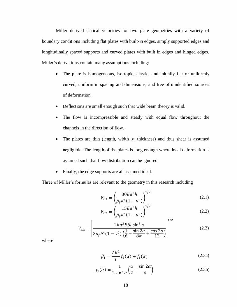
Miller derived critical velocities for two plate geometries with a variety of
boundary conditions including flat plates with built-in edges, simply supported edges and
longitudinally spaced supports and curved plates with built in edges and hinged edges.
Miller’s derivations contain many assumptions including:
The plate is homogeneous, isotropic, elastic, and initially flat or uniformly
curved, uniform in spacing and dimensions, and free of unidentified sources
of deformation.
Deflections are small enough such that wide beam theory is valid.
The flow is incompressible and steady with equal flow throughout the
channels in the direction of flow.
The plates are thin (length, width ≫ thickness) and thus shear is assumed
negligible. The length of the plates is long enough where local deformation is
assumed such that flow distribution can be ignored.
Finally, the edge supports are all assumed ideal.
Three of Miller’s formulas are relevant to the geometry in this research including
𝑉𝑐,1 = (
30𝐸𝑎3ℎ
𝜌𝑓𝑑4(1 − 𝜈2))
1/2
(2.1)
𝑉𝑐,2 = (
15𝐸𝑎3ℎ
𝜌𝑓𝑑4(1 − 𝜈2))
1/2
(2.2)
𝑉𝑐,3 = [2ℎ𝑎3𝐸𝛽1 sin
5 𝛼
3𝜌𝑓𝑏4(1 − 𝜈2) (16 −
sin 2𝛼8𝛼 +
cos 2𝛼12 )
]
1/2
(2.3)
where
𝛽1 =
𝐴𝑅2
𝐼𝑓2(𝛼) + 𝑓1(𝛼) (2.3a)
𝑓1(𝛼) =
1
2 sin2 𝛼(𝛼
2+sin 2𝛼
4) (2.3b)

19
𝑓2(𝛼) = 𝑓1(𝛼) −
1
2𝛼 (2.3c)
and 𝐸 is Young’s modulus of the plate, 𝑎 is the thickness of the plate(s), ℎ is the thickness
of the fluid channels flanking the plate(s), 𝜌𝑓 is the fluid density, 𝑑 is the width or arc
length of the plate(s), and 𝜈 is the Poisson’s ratio of the plate. In Eq. (2.3), 𝛼 is one-half
of the curved plate arc, R is the initial mean radius of curvature of the curved plate and A
is the cross sectional area of the plate per unit width. Equation (2.1) describes the critical
velocity, 𝑉𝑐,1, for a geometry with one flat plate with two fluid channels, Eq. (2.2)
describes the critical velocity, 𝑉𝑐,2, for multiple flat plates, and Eq. (2.3) describes the
critical velocity, 𝑉𝑐,3, for a multiple curved plates. The critical velocity for configurations
with one and multiple flat plates varies by a factor of 21/2
or ~1.414. This is likely caused
by multiple plates interacting with each other causing an unstable condition at a lower
velocity.
One may interpret the Miller critical velocities as the velocity at which plate
deflections will be sustained by the pressure difference created by the coolant flow as it
redistributes itself between neighboring channels. While the critical velocity does provide
some utility in defining a boundary between stable and unstable flow conditions, it does
lack significant features like the frictional pressure drop, which tends to dominate the
narrow channel flow that is characteristic in fuel assemblies. Furthermore, it ignores all
flow phenomena before and after the leading and trailing edges of the fuel plates. While
many researchers have built on Miller’s derivations in his monumental 1958 paper (and
subsequent 1960 journal article [18]), many have only suggested the addition of
multiplicative constants and/or coefficients to his formulas.

20
Miller’s colleague, Johansson, was the first of many to improve on Miller’s
critical velocity work [19]. Johansson modified Miller’s derivations to include flow
redistribution as the channels expand and contract as a result of plate deformation as well
as adding the effects of frictional pressure drops. In Miller’s derivations, he assumed only
local deformation to exist and thus flow redistribution to be negligible. Johansson also
assumed small deflections of less than ~1/2 the plate thickness so that channel areas
change by ≤ 30%. This assumption allowed Johansson to linearize his formulas.
In 1961, Rosenberg and Youngdahl replicated Miller’s analysis while including
the time dependent terms that Miller neglected [20]. They concluded for uniformly
supported plates their dynamic analysis agreed with Miller’s “neutral equilibrium”
analysis. This initial analysis did not include fluid inertia effects, however their second
analysis of plates with periodic supports did. In this second analysis, they concluded that
including the inertial effects leads to a solution where multiple critical velocities exist.
In 1963, Kane performed his own analytic study to explore how the spacing at the
inlet effected plate deflection of an array of parallel flat plates [21]. He found that around
Miller’s critical velocity small deviations in the inlet spacing caused large plate
deflections. For the analyses in this thesis, Kane’s results are rather significant since the
spacing of the plates in the models/experiments was purposely offset to quantify the
effect of the manufacturing tolerances on the stability of the plates.
Miller’s, Johansson’s, Rosenberg’s and Kane’s analyses all had the same basic
assumptions so they could complete simple first order analyses by neglecting higher
order terms. On the other hand, Scavuzzo [22] and Wambsganss [23] completed their
respective analyses in 1964 and 1967 respectively and attempted to include non-linear

21
second order effects in their derivations. Scavuzzo extended the analysis completed by C.
M. Friedrich. Friedrich, in an unpublished report, considered non-linear hydraulic loading
terms that allowed large changes in the fluid channel’s cross sectional area to occur.
More importantly, he also included the effects of manufacturing tolerances in the channel
thicknesses and concluded that these tolerances can greatly reduce the critical velocity
that causes large plate deflections. Again, like Kane’s analyses, this reaffirms that the
models/experiments in this these which purposely offset the plate will undoubtedly
demonstrate large deflections. Scavuzzo’s analysis extended Friedrich’s derivations to
include effects of fluid friction and flow redistribution in the fluid channels; however, his
results yield an integral equation that requires a numerical solver. Thus, Wambsganss’
analysis attempted to keep the simplicity of Miller’s analysis, while keeping some of the
non-linear effects explored by Friedrich and Scavuzzo.
Theoretical analyses to calculate critical velocities of parallel plate assemblies
have been of interest since at least the 1950s. As of 2014, researchers, such as Jensen [24]
and Marcum [25], are still publishing new derivations for critical velocity. In Jensen and
Marcum’s papers, critical velocities were derived for laminate composite flat and curved
plates. While the complexities added or extended to Miller’s analyses have been
extensive, his results are still the most applied and referenced in literature. Many
experimental studies have also been completed since Miller published his groundbreaking
paper.
2.2 Experiments of Hydro-Mechanical Stability
Since Miller’s definitive 1958 paper, many researchers have completed
experimental studies in an attempt to verify Miller’s and others theoretical results as well

22
as to experimentally explore hydro-mechanical stability in parallel plate assemblies.
Zabriskie completed the first experimental verifications of Miller’s critical velocities [26,
27]. He conducted extensive experiments in 1958 and 1959 to measure the critical flow
velocity of single and multiple parallel plate assemblies as well as exploring how the
length to width ratio of the plate affects the critical velocity. This included exploration of
support combs at the inlets of the multiple plate assemblies. To measure the collapse
velocity he utilized impact pressure sensors at the exit of the plates to measure sudden
changes in velocity head. Plexiglas panels were also used to allow for visual
observations. In his later 1959 study, he re-instrumented his test setup with static pressure
taps along the axial length of the plate in the hope of capturing local plate deflection. He
reported in general his experimental results agreed within ±20% of Miller’s theory, that
the critical velocity describes a point of large deflection rather than plate collapse, and
that the plate’s leading edge is most vulnerable to large deflection and that the presence
of support comb suppresses it.
Following Zabriskie’s experiments Groninger and Kane [28] conducted
experiments in 1963 on three different parallel plate assemblies using strain gages
inserted into the edges of the plates to measure deflection. Testing was completed using
both a hot and cold flow loop to explore how temperature effects plate deflection with
and without inlet support combs. Flow velocities below, at, and well above Miller’s
critical velocity were tested. At about 1.9 times the critical velocity, they observed a high
frequency flutter in the plates and that the greatest amount of deflection occurred at the
leading edge of the plate. The presence of a support comb reduced this leading edge
deflection, as Zabriskie found, while also eliminating the high frequency flutter.

23
Furthermore, they found, like Zabriskie, that the plates did not experience collapse at or
well above the critical velocity, instead they observed large plate deflections as the flow
velocity approached the critical velocity.
During the mid-1960s, Smissaert performed experiments on parallel plate
assemblies (referred to as Materials Testing Reactor fuel elements in the reference) as
part of his doctoral research at the Pennsylvania State University [29]. Both static and
dynamic deflection tests were completed. Static tests were completed on a five-plate
assembly and dynamic testing was completed on five, nine, and fifteen plate assemblies.
Deflection and pressure was monitored through strain gages mounted to two plates in the
assembly and through pressure taps mounted in the spacers between the plates. The static
tests were completed at critical velocity ratios of 1.23, 1.47, and 1.70. At each of these
velocities, it was shown that the static deflections were in the shape of a wave with
decreasing wavelength as the velocity was increased. When a support comb was added to
the leading edge of the plate assembly the strain gage measurements were very small with
a large amount of scatter thus Smissaert concluded that the support comb stabilize plate
deflection significantly. It was found that during the dynamic testing that a flutter
velocity exists and is approximately equal to two times the Miller critical velocity.
Interestingly, it was found that below the flutter velocity low amplitude traveling waves
existed in the flow direction. It was also observed that the support comb only eliminated
the high frequency flutter, but not the low frequency traveling waves.
Recent experimentation in the hydro-mechanical stability of plate assemblies was
investigated by Ho et al. in 2004 [30]. Both plate vibration and collapse were interrogated
using a simple parallel plate fuel assembly with two aluminum plates in a closed loop

24
water tunnel. The tested fuel assembly was constructed using a sandwich structure with
two 40 mm thick Perspex panels, two 1.2 mm thick aluminum plates, and three 4.3 mm
thick spacers. The assembly was instrumented with strain gages on one of the plates with
pressure taps mounted along the assembly length. The vibration testing showed that the
plate had a low frequency 4.3 Hz vibration and that the amplitude of the vibration
increased with increasing flow velocity. This low frequency vibration agrees with
observations seen by Groninger, Kane, and Smissaert, however, Ho did not mention a
presence of high frequency flutters like Groninger, Kane, and Smissaert did. This could
be because Ho kept the flow velocity at less than half of Miller’s velocity during
vibration testing whereas Groninger, Kane, and Smissaert were running well over
Miller’s velocity. Following vibration testing, Ho accessed the critical velocity of the
assembly by incrementally increasing the velocity. Instead of a sudden collapse, a gradual
buckling or collapse was observed as the velocity increased. This was also seen by
Smissaert in his experiments. Full plate collapse was observed between 11.9 and 12 m/s
or about ~78% of Miller’s velocity, interestingly, this in contrast to previous
experimental studies, which showed high frequency flutters to appear before plate
collapse. Nonetheless Ho et al.’s study shows the significance and practicality of Miller’s
study in plate-type fuel designs.
Many more recent experimental studies have being completed by Chinese
researchers with emphasis on the flow-induced vibrations (FIV). Liu et al. and Li et al. at
the North China Electric Power University investigated FIVs using one and two plate
assemblies in 2011 and 2012 [31, 32]. The plates were fixed at the corners and vibration
was monitored with a laser displacement sensor. This is in contrast to the previously

25
reviewed papers, which clamped the plates along the entire length of the plate and
typically utilized strain gages to monitor deflection and/or vibration. Both Liu and Li
reported that low frequency vibrations occurred at flow velocities below Miller’s
velocity. Additionally, in Li’s two plate tests the vibration amplitude was found to be
significantly higher than the single plate tests. Li also found that the two plate tests
showed a lower vibration frequency than the single plate tests.
While this is not a comprehensive review of the various experimental studies of
parallel plate assemblies completed since the late 1950s, the review discusses some of the
most impactful studies that are relevant to the research in this thesis. Up until recently,
utilizing theoretical and experimental techniques have been the only methods to quantify
and address the impact of how flows in high-power density reactors structurally affect
plate-type fuels. However, with the recent advances in computing power, it has been of
interest to employ numerical techniques to explore the hydro-mechanical stability of
reactor specific geometries.
2.3 Numerical Techniques
While utilizing theoretical techniques to model the hydro-mechanical stability of
fuel plates allows for quick estimates of the point of instability, their derivations often
require many assumptions in both the fluid and solid domains. These simplifications
allow the partial differential equations (PDE) that describe these domains to be solved;
however, these simplifications are likely eliminating important aspects of the PDEs
underlying physics. The use of numerical techniques allows solutions to these systems of
PDEs to be estimated without the drastic simplifications required in analytical modeling.
Unfortunately, numerical techniques have their fair share of downfalls too, including, but

26
not limited to the presence of various numerical instabilities, as well as their own
physical approximations, such as when modeling turbulent flows. Fortunately,
experimental testing provides data to validate both theoretical and numerical models as
well as provide invaluable information about how to model the physics accurately;
however, experiments are often costly especially on large scales.
As mentioned earlier, modeling hydro-mechanical stability is difficult since it
requires solving fluid and solid mechanic problems simultaneously. Typically, fluid flow
is modeled numerically in an Eulerian reference frame by dividing the geometry of
interest into finite volumes. An Eulerian reference frame works well since only the
dynamics of the fluid as it moves through the finite volumes is of interest. The shape of
the volumes at a specific reference time is generally not of interest when solving a fluid
flow problem. Conversely, when modeling the deformation of a solid it is advantageous
for the volumes within the domain to deform/move as the overall structure
deforms/moves. For this reason, finite elements in a Lagrangian reference frame are often
exploited to numerically solve structural problem. This creates difficulties when a
simultaneous fluid/structure solution is of interest since the two domains are solved most
accurately with two different descriptions of motion within continuum mechanics.
Coupling independent physical domains, such as fluid and solid domains, can be
accomplished in a few ways. The two domains can be coupled in a monolithic manner
where all the physical equations are solved simultaneously, or they can be coupled in an
independent partitioned method where each of the domains solve independently and
iteratively exchange solution data at the fluid-structure boundary. The latter partitioned
method has become a popular approach for coupling fluid and structural problems since

27
numerous methods and commercial codes exist in these respective domains. Furthermore,
these existing methods and codes are considered state of the art, and thus known to
provide excellent results in their individual domains. Thus, when coupled they should
maintain their efficiency and accuracy; however, this is not always true under certain
physical and numerical conditions [33].
Partitioned methods were first utilized to couple fluid and structure models,
known as fluid-structure interaction (FSI) model, during the mid-1970’s [33]. Some of
these first FSI models were developed to describe how an elastically deforming aircraft
wing responds within a flow field. In most FSI models, the computational domain can be
divided into two partitions, the fluid (Eulerian) and the structure (Lagrangian), as shown
in Figure 2-1’s description of an aeroelastic problem.
Figure 2-1. Three-field system of an aeroelastic problem [33].
While the Lagrangian reference frame of the structure inherently allows the
structure to move in time and space, the Eulerian reference frame of the fluid does not.
Thus, an additional piece must be added to the fluid partition of the FSI model that

28
morphs the fluid mesh around the deforming structure. In the case of aeroelastic
problems, the fluid domain can be divided into two parts, dynamic (morphing) and
stationary, since the computational domain is semi-infinite. This is in contrast to FSI
models with slender geometries where a large portion or sometimes all of the fluid mesh
must be modified as the structure deforms. Furthermore, modifying only a small portion
of the fluid mesh, since deformations are considerably smaller than the semi-infinite
domain, eliminates the likelihood of the structure deforming near or beyond the
boundaries of the fluid domain. However, aeroelastic models have stability/accuracy
issues of their own, that in some cases are relevant to FSI models of reactor cores.
Piperno and Farhat developed a novel partitioned method to estimate, with more
accuracy and stability than previous coupling methods, the aeroelasticity of aircraft wings
in transonic and supersonic flows [34]. Specifically, they developed a procedure for
analyzing the performance of partitioned methods by evaluating the buildup of artificial
energy at the fluid/structure interface, developed as a byproduct of the inherent
staggering process of partitioned methods. This numerically produced energy leads to
loss in time-accuracy and numerical stability since momentum and energy at the interface
is no longer conserved. Their derivations helped evaluate previously proposed partitioned
methods for use in aeroelastic problems with semi-infinite computational domains.
However, when the geometry is slender and bounded by rigid walls, as in geometries
within reactor cores, a runaway buildup of artificial energy (developed from the coupling
scheme’s staggered process) could occur and without the dissipative property of a
compressible flow in a semi-infinite domain, this buildup could cause the model to go

29
unstable. This is particularly true when the fluid and structure domains exchange
information at the fluid/structure interface only once per time step.
Most aeroelastic problems utilize a partitioned method that iterates the fluid and
solid domains only once per time step, known as a loose (explicit) coupling scheme, as in
the case of Piperno and Farhat [34]. In contrast, strongly (semi-implicit) coupled schemes
iterate multiple times within a time step. Loose coupling is advantageous from a
computational efficiency standpoint, but unfortunately, outside of aeroelastic problems
loose coupling is largely unstable. Instabilities occur most frequently when the densities
of the fluid and the structure are similar and/or when the geometry is slender in nature
[35, 36]. Another more severe instability occurs when incompressible flows are coupled
with thin and light structures. The instability has been named the “added-mass effect”
since it has been traced back to how at the fluid/structure interface the incompressible
fluid acts as an additional mass on the structure. This added-mass effect is amplified with
loose coupling schemes since the fluid forces rely upon a predicted structural
displacement rather than the correct displacements, thus energy at the fluid/structure
interface is unlikely to be conserved. A buildup of this excess energy yields an increased
probability of instability occurring.
Causin et al. completed work on these types of instabilities that plague loosely
coupled schemes, specifically in the context of blood flowing through an artery [35].
Nobile found during his Ph.D. research that numerical instabilities occur when the
density of the structure, or artery, drops below a certain threshold and/or when the length
of the domain or artery increased beyond a certain threshold [37]. For stability analysis
purposes, Causin simplified Nobile’s hemodynamic FSI models without eliminating the

30
instability-inducing added-mass effects. Instability conditions/criteria were developed by
deriving an added-mass operator and using its maximum eigenvalue. The instability
conditions verified empirical observations seen in Nobile’s nonlinear hemodynamic
models. This included proving that instability increases as the domain becomes more
slender, i.e. as the length increases and/or the radius decreases, and/or as the
structure/fluid density ratio decreases. While, these analyses are important from a
hemodynamic standpoint they also pertain to reactor core geometries where the
structures, fuel plates or pins, are very slender in nature and are mechanically stimulated
by incompressible fluids, such as water or liquid sodium.
Following the work of Causin et al., Forester et al. further investigated the added-
mass effect of incompressible flows by building on Causin’s work [36]. Specifically, they
explored how the temporal discretization affects the stability of loosely coupled schemes
by deriving an added-mass operator similar to Causin’s operator. The maximum
eigenvalue of this operator as well as the fluid/structure density ratio appear in their
stability conditions. This thereby proves that any loosely coupled algorithm, even the
most stable, has a mass density ratio that will cause instability at some point during the
simulation. Although, most importantly, they established that the maximum eigenvalue of
their added-mass operator increases as the time step decreases, thereby explaining why
stabilized FSI models of incompressible flows become severely unstable with very small
time steps. This proves that the added-mass effect effectively creates a lower bound on
the time step of conditionally stable FSI models that utilize a loose coupling scheme.
Furthermore, since loosely coupled schemes are inherently explicit an upper bound on the
time step will likely also exist, due to the Courant-Freidrichs-Lewy (CFL) condition [38].

31
While these aforementioned numerical studies stress the difficulties of
numerically simulating the interaction of a fluid and a structure the problem is not
impossible. The next three chapters detail the fluid model (Chapter 3), the structure
model (Chapter 4) and the schemes for coupling them together (Chapter 5). Both Chapter
3 and 4 include how the numeric models were built, mesh studies, and analytic models
for checking the accuracy of the numeric models. Chapter 3 also includes a study that
explored a suite of turbulence models by comparing their solutions to the solution of a 1D
analytic model. The coupling scheme utilized to couple the fluid and structure models is
detailed in Chapter 5 as well as outlines for the various empirical stability studies
completed with the FSI models. These stability studies include exploring the effect of the
time step, the slenderness of the computational domain, and the fluid/structure density
ratio on stability. Results of these stability studies are in Chapter 6 as well as plate
deflection results at a range of velocities for comparing to the experiment in Chapter 7 for
benchmarking purposes. Chapter 7 also includes a description of a new high precision
positioning system for the experiment’s laser displacement sensors to help facilitate
closer matching of future FSI models with the experiment. Finally, Chapter 8 includes
parametric studies of more prototypic curved plates to reveal the influence of curvature.

32
CHAPTER 3 - MODELING OF FLUID FLOW AROUND FUEL PLATES
The previous chapter dove into a brief history of how the interaction of a fluid and
a structure has been modeled and tested over the past half century, particularly in the
context of parallel plate assemblies. Furthermore, previous numerical FSI studies were
explored in both the context of a compressible flow over an airfoil and an incompressible
flow of blood through an artery to highlight the difficulties associated with building and
stabilizing FSI models of parallel plate assemblies. This chapter introduces the fluid flow
partition of the interested FSI model that includes mesh/turbulence studies as well as a
comparison to a 1D analytic model.
3.1 Fluid Geometry
A generic diagram of the fluid model is shown in Figure 3-1. This geometry will
be utilized in both numeric and analytic modeling and is based off the experimental
geometry that is detailed in Chapter 7.
Table 3-1 details the geometric
parameters shown in Figure 3-1 and
Table 3-2 details the fluid properties
for the incompressible flow of water.
The thicknesses of the two channels
flanking the voided region (where the
plate would reside if it were included
in the fluid model) vary from model to
model. In the majority of the fluid
models, the channels will either be
Figure 3-1. Fluid model geometry (not to scale).

33
2.03 mm (80 mils) and 2.54 mm (100 mils) or they will both be 2.29 mm (90 mils) thick.
In all models a known velocity will be specified at the inlet (top of Figure 3-1) and a
known pressure will be specified at the outlet (bottom of Figure 3-1). Finally, all walls
(thick black lines in Figure 3-1) will be specified as no-slip ‘smooth’ rigid walls.
Table 3-1. Geometric parameters for fluid models.
𝒂 1.02 mm (40 mils)
𝒃 2.03 to 2.29 mm (80 to 90 mils)
𝒄 2.29 to 2.54 mm (80 to 100 mils)
𝒅 (𝒊𝒏𝒕𝒐 𝒑𝒂𝒈𝒆) 110.3 mm (4.342”)
𝑳𝒊𝒏𝒍𝒆𝒕 190.5 mm (7.5”)
𝑳𝒑𝒍𝒂𝒕𝒆 647.7 mm (25.5”)
𝑳𝒐𝒖𝒕𝒍𝒆𝒕 76.20 mm (3”)
Table 3-2. Fluid properties for water.
Density 997.561 𝑘𝑔/𝑚3
Dynamic Viscosity 8.8871 × 10⁻⁴ 𝑃𝑎 ∗ 𝑠
The velocity specified at the ‘Velocity Inlet’ of Figure 3-1 is based off the average
channel velocity, 𝑉𝑎𝑣𝑔,𝑐ℎ , within the channels flanking the ‘Voided Region’. Using the
conservation of mass and the fact that the flow is incompressible the inlet velocity, 𝑉𝑖𝑛𝑙𝑒𝑡 ,
can be calculated using:
𝑉𝑖𝑛𝑙𝑒𝑡 =
𝑏 + 𝑐
𝑎 + 𝑏 + 𝑐𝑉𝑎𝑣𝑔,𝑐ℎ (3.1)
It should be noted, all occurrences of the term ‘flow velocity’ in this thesis will be in
reference to the average channel velocity, 𝑉𝑎𝑣𝑔,𝑐ℎ , not the inlet velocity, 𝑉𝑖𝑛𝑙𝑒𝑡. Equation
(3.1) is also used in the curved plate models in Chapter 8. The error of using Eq. (3.1) for
specifying the average channel velocity in the curved plate models is < 0.1%.

34
3.2 Analytic Fluid Model
An analytic model for computing pressure drop through the geometry in Figure 3-
1 was developed for validation purposes. The 1-dimensional (1D) analytic model
assumes:
The flow is incompressible, fully developed, and turbulent.
The flow equally splits at the axial centerline of the plate at both the
leading and trailing edges.
All walls are rigid and smooth.
Gravity is ignored.
The flow through the geometry will
experience both reversible and
irreversible (including minor and major)
losses. The minor and major losses are
shown by the “flow resistances” in
Figure 3-2. For this geometry, the minor
losses are from the expansion and
contraction at the leading and trailing
edges of the plate and the major losses
are from frictional losses. In Figure 3-2
the shorter red “flow resistances’ signify
minor losses and the longer blue “flow
resistances” signify major losses. To start, Bernoulli’s equation:
𝑃𝑖𝑛𝜌+𝑉𝑖𝑛
2
2+ 𝑔𝑧𝑖𝑛 =
𝑃𝑜𝑢𝑡𝜌
+𝑉𝑜𝑢𝑡
2
2+ 𝑔𝑧𝑜𝑢𝑡 (3.2)
Figure 3-2. Minor and major losses through the
flow geometry.

35
which is utilized to represent the pressure drop that occurs due to the changing area at the
leading and trailing edges of the plate. Eq. (3.2) can be simplified since the inlet and
outlet plenum areas are equal the velocity at these points will also be equal. However, a
reversible loss will occur at the leading and trailing edges of the plate due to the
increase/decrease in velocity. While this loss will be recovered at the expansion,
including it will be important when comparing the analytic and numeric axial pressure
profiles. When accounting for major/minor losses Eq. (3.2) becomes:
∆𝑃𝑖𝑛−𝑜𝑢𝑡 = 𝑃𝑖𝑛 − 𝑃𝑜𝑢𝑡 =∑∆𝑃𝑚𝑎𝑗𝑜𝑟 +∑∆𝑃𝑚𝑖𝑛𝑜𝑟 (3.3)
3.2.1 Frictional and Minor Losses
The pressure drops due to minor losses through the geometry shown in Figure 3-1
and Figure 3-2 emerge from the expansion and contraction at the leading and trailing
edges of the plate. As mentioned earlier, it is assumed that the flow splits at the axial
centerline of the plate as shown in Figure 3-3. Minor losses in internal flow are largely
given as coefficients denoted by k since the values are commonly derived empirically.
Figure 3-3. Parameters for computing contraction and expansion losses.

36
The minor loss due to contraction at the plate’s leading edge, 𝑘𝑐𝑜𝑛𝑡𝑟𝑎𝑐𝑡𝑖𝑜𝑛, is computed
using:
𝑘𝑐𝑜𝑛𝑡𝑟𝑎𝑐𝑡𝑖𝑜𝑛 = 0.42(1 −
𝑑2
𝐷2) (3.4)
where D and d are the flow diameters before and after the contraction, respectively.
Equation (3.4) was found in Fluid Mechanics by White and was theoretically derived
using control volume theory [40]. Since the flow is through rectangular ducts, the
hydraulic diameter is utilized and is computed using:
𝐷ℎ =
4𝐴
𝑃 (3.5)
where A and P are the flow area and wetted perimeter at a particular cross section of the
flow. In a similar way to the contraction losses the loss due to the expansion at the
trailing edge of the plate, 𝑘𝑒𝑥𝑝𝑎𝑛𝑠𝑖𝑜𝑛, is computed using:
𝑘𝑒𝑥𝑝𝑎𝑛𝑠𝑖𝑜𝑛 = (1 −
𝑑2
𝐷2)
2
(3.6)
where d and D are the flow diameters before and after the expansion, respectively.
Equation (3.6) was also found in Fluid Mechanics by White, but this k loss was
empirically derived instead of theoretically. The k losses in Eqs. (3.4) and (3.6) were used
to estimate pressure drop using:
∆𝑃𝑚𝑖𝑛𝑜𝑟 =
1
2𝑘𝑙𝑜𝑠𝑠𝜌𝑓𝑉
2 (3.7)
where 𝜌𝑓 is the fluid density. Equation (3.7) is nothing more than the loss coefficient
multiplied by the dynamic pressure. It should be noted that the velocity in Eq. (3.7) is
always the velocity through the smaller portion of the expansion/contraction geometry.

37
The viscous effects that are caused by walls in an internal flow produce losses in
the flow’s energy. They are called frictional losses and they contribute the highest
amount of energy loss through Figure 3-1’s geometry. The pressure drop due to frictional
losses is calculated using:
∆𝑃𝑚𝑎𝑗𝑜𝑟 = 𝑓
𝜌𝑓𝐿𝑉2
2𝐷ℎ (3.8)
where L is the length of the pipe or duct, and f is the Darcy friction factor. The friction
factor, f, depends on the Reynolds Number, 𝑅𝑒𝑑, and the wall roughness height. The
Reynolds Number is computed using
𝑅𝑒𝑑 =
𝜌𝑓𝑉𝐷ℎ𝜇
(3.9)
where 𝜇 is the fluid’s dynamic viscosity. The Reynolds number is used to help judge if a
particular flow is laminar, transitional, or turbulent by providing the ratio of inertial
forces to viscous forces within a flow. For the geometry, fluid properties, and flow
conditions in this model the flow is fully turbulent. Thus, the friction factor, f, can be
computed using the Colebrook equation
1
𝑓1/2= −2.0log (
휀/𝑑
3.7+
2.51
𝑅𝑒𝑑𝑓1/2) (3.10)
where 휀 is the wall roughness height [39]. Since Eq. (3.10) is transcendental, an iterative
technique, such as the Newton-Raphson method, is required to solve for f.
3.2.2 Case of Unequal Flow Channels
Two cases exist for the geometry in Figure 3-1. The first, when the plate is
centered in the geometry, which yields equal fluid channels and the second, when the
plate is shifted in the geometry, which yields unequal channels. While the analytic
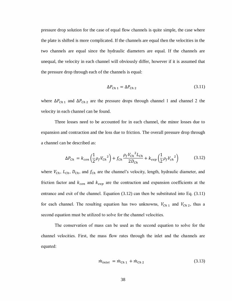
38
pressure drop solution for the case of equal flow channels is quite simple, the case where
the plate is shifted is more complicated. If the channels are equal then the velocities in the
two channels are equal since the hydraulic diameters are equal. If the channels are
unequal, the velocity in each channel will obviously differ, however if it is assumed that
the pressure drop through each of the channels is equal:
∆𝑃𝐶ℎ 1 = ∆𝑃𝐶ℎ 2 (3.11)
where ∆𝑃𝐶ℎ 1 and ∆𝑃𝐶ℎ 2 are the pressure drops through channel 1 and channel 2 the
velocity in each channel can be found.
Three losses need to be accounted for in each channel, the minor losses due to
expansion and contraction and the loss due to friction. The overall pressure drop through
a channel can be described as:
∆𝑃𝐶ℎ = 𝑘𝑐𝑜𝑛 (
1
2𝜌𝑓𝑉𝐶ℎ
2) + 𝑓𝐶ℎ𝜌𝑓𝑉𝐶ℎ
2𝐿𝐶ℎ2𝐷𝐶ℎ
+ 𝑘𝑒𝑥𝑝 (1
2𝜌𝑓𝑉𝑐ℎ
2) (3.12)
where 𝑉𝐶ℎ , 𝐿𝐶ℎ, 𝐷𝐶ℎ, and 𝑓𝐶ℎ are the channel’s velocity, length, hydraulic diameter, and
friction factor and 𝑘𝑐𝑜𝑛 and 𝑘𝑒𝑥𝑝 are the contraction and expansion coefficients at the
entrance and exit of the channel. Equation (3.12) can then be substituted into Eq. (3.11)
for each channel. The resulting equation has two unknowns, 𝑉𝐶ℎ 1 and 𝑉𝐶ℎ 2, thus a
second equation must be utilized to solve for the channel velocities.
The conservation of mass can be used as the second equation to solve for the
channel velocities. First, the mass flow rates through the inlet and the channels are
equated:
�̇�𝑖𝑛𝑙𝑒𝑡 = �̇�𝐶ℎ 1 + �̇�𝐶ℎ 2 (3.13)

39
where �̇� = 𝜌𝑓𝑉𝐴 (3.14)
where �̇�𝑖𝑛𝑙𝑒𝑡 , �̇�𝐶ℎ 1, and �̇�𝐶ℎ 2 are the mass flow rates through the inlet plenum and the
two channels. Since the flow is assumed to be incompressible Eqs. (3.13) and (3.14) can
yield:
𝑉𝐶ℎ 2 = 𝑉𝑖𝑛𝑙𝑒𝑡
𝐴𝑖𝑛𝑙𝑒𝑡𝐴𝐶ℎ 2
− 𝑉𝐶ℎ 1𝐴𝐶ℎ 1𝐴𝐶ℎ 2
(3.15)
Using Eqs. (3.11) and (3.12) with Eq. (3.15) the equation
1
2𝜌𝑓𝑉𝐶ℎ1
2 (𝑘𝑐𝑜𝑛,𝐶ℎ1 + 𝑓𝐶ℎ 1𝐿𝐶ℎ1𝐷𝐶ℎ1
+ 𝑘𝑒𝑥𝑝,𝐶ℎ1)
=1
2𝜌𝑓(𝑉𝑖𝑛𝑙𝑒𝑡
𝐴𝑖𝑛𝑙𝑒𝑡𝐴𝐶ℎ 2
−𝑉𝐶ℎ 1𝐴𝐶ℎ 1𝐴𝐶ℎ 2
)2
(𝑘𝑐𝑜𝑛,𝐶ℎ2 + 𝑓𝐶ℎ2𝐿𝐶ℎ2𝐷𝐶ℎ2
+ 𝑘𝑒𝑥𝑝,𝐶ℎ2) (3.16)
can be used to compute channel 1’s velocity, 𝑉𝐶ℎ 1. While the solution to Eq. (3.16)
appears to be simple, the friction factors cause the equation to be transcendental. A
Newton-Raphson solver was written to numerically solve the for the channel velocity,
𝑉𝐶ℎ 1. Once this velocity is known channel 2’s velocity can easily be found using Eq.
(3.15). The code written for solving the above equations for pressure is in Appendix 3.
Now that the velocities in both channels are known, the full pressure profile can
be constructed as shown in Figure 3-4. Since the pressure is assumed 0 Pa at the outlet,
the construction of the pressure profile will start here. Technically the pressure at the
outlet is unknown, but the pressure here is also irrelevant since the pressure at this point
will only equally shift the pressure values throughout the model. The pressure will
increase from the outlet to the plate’s trailing edge as a result of the irreversible frictional
pressure drop through the outlet plenum. It is then assumed at the trailing edge the
pressure will drop slightly from the reversible recovery due to the area change and
increase due to the irreversible loss due to the expansion. The pressure will then linearly

40
increase from the irreversible frictional loss through the channels. At the leading edge,
the pressure will rise both reversibly and irreversibly due to the area increase and the
contraction, respectively. From there the pressure will linearly increase through the inlet
plenum from the irreversible loss due to friction.
Figure 3-4. 1D analytic model’s axial pressure profile solution at 8 m/s.
3.3 Numeric Fluid Model
The coolant flow around the flat plate in Figure 3-1 was simulated in the
commercial CFD code Star-CCM+. A basic process exists that must be followed to solve
a fluid mechanics problem with CFD. First, a solid geometry of the fluid must be created.
This geometry is then discretized into a grid or mesh. Creating the mesh can be the most
challenging part of building any type of numeric model and can be particularly difficult
when building a mesh for a CFD model. A detailed description of the mesh building
process is in Section 3.3.2. Once the mesh is created, the correct physics models must be
chosen. Choosing the physics models for a CFD model should be closely tied with how

41
the mesh is created. Vastly different solutions can be found depending on the specific
physics models that are utilized with a given fluid mesh. This is especially true when the
flow is turbulent and turbulence models are required. Based on the chosen physics
models, the correct boundary conditions must then be set. Finally, “derived parts” such as
line and point probes are created for visualizing the solution as is progresses and for post
processing. Reports, monitors, stopping criteria, and plots/scenes are also created for
similar reasons. Details on some of these CFD model-building steps are described in the
subsequent subsections.
3.3.1 Geometry, Boundary Conditions, and Stopping Criteria
Figure 3-5 shows the fluid geometry in Star-CCM+ for the coolant flow around a
flat plate. The ‘Velocity Inlet’ surface was set using Eq. (3.1), the ‘Pressure Outlet’
surface was set to 0 Pa, and all the rest of
the surfaces, including the voided region
surfaces, were prescribed as no-slip
‘smooth’ walls for all models in Star-
CCM+. The flow channels for the
preliminary CFD models had equal
thicknesses of 2.29 mm (90 mils). The
channels were set equal so the CFD model
could be easily benchmarked to the
simpler and likely more accurate 1D
analytic model developed in Chapter 3.2.
Figure 3-5. Fluid geometry in Star-CCM+.

42
Stopping criteria were added to the CFD models by creating reports and monitors
of specific values in fluid solution. For this CFD model, reports were created to calculate
the maximum, minimum, and average pressures and wall shear stresses on the voided
region’s surfaces. These surfaces are where the solution is most pertinent especially when
the CFD model is coupled to the solid model since the two models will exchange data at
these surfaces. These pressure and wall shear stress reports were then used to create
monitors. Monitors keep track of the report’s calculations so plots and stopping criteria
can be created. The plots give the user the ability to keep track of the solution as it
progresses. Six separate criterions are created for each of the six monitors. All six criteria
have to be satisfied to move on to the next time step. To satisfy the criteria the pressure
and wall shear stress solutions must not change within 1 Pa for 25 consecutive iterations
or until 350 iterations are reached.
3.3.2 Fluid Mesh
The fluid mesh was not created within Star-CCM+’s environment, but rather in
Abaqus’. The Abaqus user interface allows for a much higher control of how cells are
placed on geometries. This is in contrast to the meshing tools/algorithms in Star-CCM+
which are tailored towards meshing irregular geometries using automated algorithms.
Attempts were made to create meshes using Star-CCM+, but the algorithms did not work
well on the high aspect ratio geometry and tended to be computationally expensive.
Initial meshes created in Star-CCM+ were adequate through most of the model, but
through the thickness of the channels, the mesh would be too coarse (approximately 5
cells). The accuracy of the fluid solution through these channels will be extremely
important when the model is coupled to the solid model. When the cell sizes through the

43
channel thicknesses were decreased, the mesh densities became approximately
10,000,000 cells, which is too dense for the computational resources currently available.
Thus, the mesh was created in Abaqus and was easily imported into Star-CCM+ using an
Abaqus input file, which contains the locations of the nodes in the mesh.
The first step for building the mesh in Abaqus was to build solid geometry. The
geometry for the plate was created such that the plate geometry could be used to cut away
the voided region in Figure 3-1 from a bulk fluid block. The bulk fluid block is just a thin
rectangle with dimensions of (𝑎 + 𝑏 + 𝑐) by (𝐿𝑖𝑛𝑙𝑒𝑡 + 𝐿𝑝𝑙𝑎𝑡𝑒 + 𝐿𝑜𝑢𝑡𝑙𝑒𝑡) by 𝑑. The newly
cut Un-Partitioned geometry shown in Figure 3-6 was then partitioned at the
leading/trailing edges, and on the front/back sides of the plate along the y-axis as shown
by the red solid lines on the right side of Figure 3-6. These four partitions allowed a
structured mesh to be created. Notice that the Un-Partitioned geometry in Figure 3-6 is
yellow and the Partitioned geometry is green. In Abaqus, green geometry signifies a
structured mesh can be created, whereas a yellow geometry signifies an unstructured
mesh can be created. Four additional partitions were also created at defined distances
from the walls along the y-axis as shown by the red dashed lines in Figure 3-6 for a total
of 8 partitions. These additional partitions were created so the thicknesses of the wall
bounding cells could be controlled. The thicknesses of these wall-bounding cells will
dictate the wall y+ values in the fluid solution.
The fully partitioned geometry on the right side of Figure 3-6 was then “seeded”
on the edges created by these partitions. “Seeding” tells Abaqus where and how to place
the cells on the edges of the geometry. The structured mesh was then created and an input
file was written for importing into Star-CCM+ as shown in Figure 3-7.

44
Figure 3-6. Fluid geometry in Abaqus both un-partitioned and partitioned.
A mesh independence study was completed on the mesh shown in Figure 3-7 to
assure this fluid mesh’s solution was independent of its mesh size. Table 3-3 includes all
the parameters varied for each of the meshes explored. Figure 3-8 shows some of these
parameters on the mesh excluding the Inlet and Outlet Lengths. The Inlet and Outlet
Lengths are the distances from the leading and trailing edges of the plate to the inlet and
outlet of the geometry, respectively. The spacing of the cells along the Inlet, Outlet, and
Plate lengths were biased towards the ends of these lengths. The bias was set to 4:1 such
that the cells near the ends of these lengths are ¼ the size of the cells at the center of the
lengths. This is an effort to capture the contraction/expansion effects at the
leading/trailing edges of the plate. There was not a bias included through the thicknesses
of the channels (Ch1/Ch2 Cells), however the thickness of the near wall cells was
specifically set (hence the previously mentioned partitions) to assure the wall y+ values
remained constant for each mesh. Note that the number of cells was also increased
through the Z direction of the inlet/outlet plenums at a similar rate as the other parameters

45
and are reflected in the mesh density values shown in Table 3-3. To quantify how the
solution changed from mesh to mesh the % change in values such as the inlet pressure
was tracked using:
𝑈% 𝐶ℎ𝑎𝑛𝑔𝑒 =
𝑈𝑐𝑢𝑟𝑟𝑒𝑛𝑡 − 𝑈𝑝𝑟𝑒𝑣𝑖𝑜𝑢𝑠𝑈𝑝𝑟𝑒𝑣𝑖𝑜𝑢𝑠
× 100 (3.17)
where 𝑈𝑐𝑢𝑟𝑟𝑒𝑛𝑡 is the current mesh’s solution, 𝑈𝑝𝑟𝑒𝑣𝑖𝑜𝑢𝑠 , is the previous, less dense,
mesh’s solution, and 𝑈% 𝐶ℎ𝑎𝑛𝑔𝑒 is the % change in the solution between the two meshes.
Figure 3-7. Imported mesh in Star-CCM+.

46
Table 3-3 Details of meshes in Star-CCM+ mesh independence study.
Number of Cells Along Edge
Plate Length Ch1/Ch2 Cells Inlet Length Outlet Length Mesh Density
Mesh 1 120 8 35 15 183,300
Mesh 2 144 10 42 18 276,900
Mesh 3 173 12 51 22 402,740
Mesh 4 208 15 62 27 608,075
Mesh 5 255 18 75 30 897,000
Mesh 6 306 22 90 36 1,317,420
Mesh 7 368 27 108 36 1,890,720
Mesh 8 442 33 130 44 2,755,740
Figure 3-8. Fluid mesh in Star-CCM+ with parameters for the mesh independence study.
3.3.3 Physics Models
Choosing the correct physics for a CFD model can be one of the most difficult
tasks when building a CFD model. Table 3-4 lists the basic physics models chosen for
the CFD models. The flow in the CFD model is assumed an incompressible liquid three-
dimensional flow; however, choosing some of the other physics models is not as obvious.
An implicit unsteady solver was chosen since once the CFD model is utilized in a
coupled FSI model an unsteady solver will be required. A segregated flow model solves
the conservation of mass and momentum equations in an uncoupled manner using a
SIMPLE-esque (Semi-Implicit Method for Pressure-Linked Equations) algorithm
whereas the coupled flow model solves the flow equations simultaneously [40, 41]. A

47
segregated flow solver was chosen over the coupled solver because the segregated solver
was faster. A coupled flow solver is usually only beneficial when the flow is
compressible and has dominant source terms such as adverse pressure gradients [40].
Since the coolant’s flow around the plate is fully turbulent, a turbulence model
must be utilized to obtain accurate fluid solutions. Numerous turbulence models have
been developed since the advent of CFD with the most popular being the Reynolds-
Averaged Navier Stokes (RANS) variety. A study comparing turbulence models was
completed with a small suite of RANS models. Table 3-5 lists the RANS models that
were used during the turbulence model study.
Table 3-4. Physics models used in Star-CCM+.
Three Dimensional
Implicit Unsteady
Liquid
Segregated Flow
Constant Density
Turbulent
Reynolds-Averaged Navier Stokes
Various Turbulence Models
Various Turbulent Flow Wall Treatments
Table 3-5. RANS turbulence models explored.
High Y+ Low Y+ All Y+
Standard K-Epsilon Tested NA NA
Realizable K-Epsilon Tested NA NA
Realizable K-Epsilon Two Layer NA NA Tested
Standard (Wilcox) K-Omega Tested Not Tested Tested
SST (Menter) K-Omega Tested Not Tested Tested
3.3.4 Turbulence Modeling Wall Treatments
Turbulence models need certain assumptions regarding how to model the near-
wall solution; these assumptions are called wall treatments. Included in Star-CCM+’s
turbulence models are three types of wall treatments, namely the low y+, the high y+, and

48
a hybrid, the all y+. However, not all wall treatments are available for each specific
turbulence model.
The main advantages of the high y+ wall treatment over that of the low y+ wall
treatment are fast convergence rates and enhanced numerical stability. However, the high
y+ wall treatment includes a few extra modeling assumptions that the low y+ wall
treatment lacks. These include assuming a velocity profile that is dependent on semi-
empirical correlations. Namely, the logarithmic overlap layer first published by C.B.
Millikan in 1937 as well as the law of the wall first published by Theodore von Kármán
in 1930 [39, 42]. The logarithmic overlap layer or log-law is described by:
𝑢+ =
1
𝜅ln(𝑦+) + 𝐵, 𝜅 ≈ 0.41 𝑎𝑛𝑑 𝐵 ≈ 5.0 (3.18)
and the law of the wall is described by:
𝑢+ = 𝑦+ =
𝑦𝑢∗
𝜐 , 𝑢∗ = (
𝜏𝑤𝜌𝑓)
1/2
(3.19)
The symbol 𝑢∗ is called the friction velocity, but only because it has units of
distance per unit time since it is not actually a flow velocity. The non-dimensional
distance from the wall, 𝑦+, is equal to 𝑢+, the non-dimensional velocity perpendicular to
the wall, although this equation is only valid up until about 𝑦+ = 5 where Eq. (3.18) takes
over at about 𝑦+ = 30. These two regions are called the viscous sublayer and log law
regions respectively. The region where neither equation is valid, from about 5 < 𝑦+ <
30, is called the buffer region. All three of these regions are shown in Figure 3-9, which
also includes how Eq. (3.19), the blue solid curve, and Eq. (3.18), the red dashed curve
overlap each other in the buffer region [39]. High y+ wall treatments use these semi-
empirical relations to approximate the turbulent quantities, such as the turbulent kinetic

49
energy, 𝑘, and the turbulent dissipation rate, 휀, in the 𝑘-휀 turbulence model and the
turbulent kinetic energy and specific dissipation rate, 𝜔, in the 𝑘-𝜔 turbulence model,
near the wall.
Figure 3-9. Law of the wall and log law showing the regions of the velocity profile near the
wall.
Two main assumptions are made when wall functions, i.e. high y+ wall treatment,
are utilized: (1) the near wall velocity distribution is assumed to follow the log-law,
which allows properties of the turbulence near the wall to be estimated, and (2) it is
assumed the centroids of wall-bounding cells are within the log law region of Figure 3-9
[40]. This allows coarse meshes to be utilized since many cells do not need to be placed
close to the wall to fully resolve the velocity profile.
Figure 3-10 illustrates how a near wall mesh should look if a high y+ wall
treatment is utilized. Notice the centroids of the wall-bounding cells are within the log-
law region of the velocity profile thus this mesh would yield wall y+ values > 30, a rule
of thumb when creating meshes for wall function use. The upper limit of wall y+ values

50
when using wall functions varies. Some factors that affect the upper limit are the
Reynolds number and if pressure gradients dominate the fluid solution [40]. If the wall
y+ values are too high, potential errors could arise, therefore it is recommended for wall-
bounded cells to stay within the range of 30 ≤ 𝑦+ ≤ 50. It is apparent that the mesh
density will be considerably less when utilizing high y+ wall treatments since many cells
do not have to reside in the buffer and viscous sublayer regions like they do in low y+
wall treatments.
Figure 3-10. Comparing near wall meshes of high y+ and low y+ wall treatments, red line
signifies the velocity profile near the wall and the yellow point is the near wall cell centroid.
The low y+ wall treatment assumes the turbulence model is valid throughout the
entire boundary layer including the viscous sublayer. Thus, to obtain an accurate fluid
solution several cells must be placed near the wall as shown in Figure 3-10 so the model
can properly resolve the fluid solution in the viscous sublayer. A sufficiently refined
mesh will yield solutions with wall y+ values around 1, a rule of thumb for low y+ wall
treatments. The major drawback, as mentioned earlier, is the increase in mesh density,
and therefore computational expense especially for high Reynolds number models where
the viscous dominated region of the boundary layer is very thin.
The final wall treatment included in Star-CCM+ is the all y+ wall treatment. This
hybrid model attempts to use the high y+ wall treatment where the mesh is coarse and the

51
low y+ wall treatment where the mesh is sufficiently fine. It also attempts to obtain
reasonable solutions for wall bounding cells that are within the buffer region of the
boundary layer using:
𝑢+ =
1
𝜅ln(1 + 𝜅𝑦+) + 𝐶 (1 − exp (−
𝑦+
𝑦𝑚+) −
𝑦+
𝑦𝑚+ exp (−𝐷𝑦
+)) (3.20)
where
𝐶 =
1
𝜅ln (
𝐸
𝜅) (3.20a)
𝐷 = 0.5 (
𝑦𝑚+𝜅
𝐶+1
𝑦𝑚+) (3.20b)
which is Reichardt’s blended wall law [41]. The y+ value at the intersection of the
viscous and fully turbulent regions is 𝑦𝑚+, which is solved for iteratively. The ability of
the all y+ wall treatment to obtain reasonable solutions in the buffer region of the velocity
profile using Eq. (3.20) makes it an attractive model for meshes where the wall y+ values
are difficult to control due to irregular or morphing geometries.
3.4 Results of Preliminary Fluid Model Studies
Two studies were conducted with the numeric model including the turbulence
model and mesh independence studies. The turbulence model study was completed first
to find a turbulence model that agreed well with the 1D analytic model developed in
Section 3.2. The turbulence model that agreed most closely with the 1D analytic model
was then utilized in the mesh independence study.
3.4.1 Turbulence Model Study Results
Five different RANS turbulence models were explored for this study including the
standard, realizable, and realizable Two-Layer forms of the 𝑘-휀 model, and the standard

52
(Wilcox) and Shear Stress Transport (SST) (Menter) forms of the 𝑘-𝜔 model. Within
these models are three wall treatments, although not all of these turbulence models have
access to each wall treatment. Table 3-5 shows which wall treatments are available for
each turbulence model. During the study the low y+ wall treatment was not explored,
however a model with a high-density mesh was completed. This model included a
sufficiently refined mesh that resolved the fluid solution through the entire boundary
layer. Its results are shown at the end of this chapter.
All models were run to a steady state with an average channel velocity of 8 m/s
using the mesh shown in Figure 3-7 and Figure 3-8, i.e. Mesh 5 in Table 3-3. Table 3-6
details the average y+ values this mesh yields. The average was taken from y+ values on
the surfaces of the plate and the channel walls. All averages are > 30, however specific
values near the leading edge of the plate where stagnation and likely separation occurs
the y+ values are < 30. This situation is acceptable near stagnation and/or separation and
y+ values as low as 12 are unlikely to cause significant error with high y+ wall treatments
[41]. Furthermore, the turbulence models that utilize an all y+ wall treatment utilize the
blended wall law, Eq. (3.20), which allows it to obtain reasonable solutions when y+
values are within the buffer region of the velocity profile.
Table 3-6. Wall y+ values of near wall cells on the channel walls and plate surface.
Average y+ Values of Near Wall Cells
High Y+ All Y+
Standard
𝒌 − 𝜺 37.18 -
Realizable
𝒌 − 𝜺 36.68 -
Realizable Two Layer
𝒌 − 𝜺 - 36.54
Standard (Wilcox)
𝒌 −𝝎 38.16 37.98
SST (Menter)
𝒌 −𝝎 37.58 37.77

53
Each turbulence model was compared to the analytic model using the overall
pressure drop through the geometry and the axial profile of the pressure as shown in
Figure 3-4. First, the pressure drop with each turbulence model was extracted so it could
be compared to the pressure drop from the analytic model by calculating the percent
difference between the two values using Eq. (3.17). Then the axial pressure profile from
each turbulence model was compared to the axial pressure profile from the analytic
model, which is shown in Figure 3-4. The pressure data was extracted from the numeric
models by creating a line probe centered in one of the channels. The probes extended
from the inlet to the outlet.
Table 3-7 shows the pressure drop for each turbulence model using Mesh 5 as
well as the % difference from the analytic model. The pressure drop calculated using the
analytic model was 1.18 kPa. It is apparent the realizable 𝑘-휀 Two Layer model with an
all y+ wall treatment agrees best with the analytic model since its predicted inlet pressure
differed from the analytic model by only 0.32%. Overall, the 𝑘-휀 suite performed better
than the 𝑘-𝜔 suite. Specifically, the realizable 𝑘-휀 models (high y+ and two layer all y+)
showed the best agreement with 2.4% and 0.32% difference from the analytic model.
Table 3-7. Pressure drop for each turbulence model with % difference from analytic model.
High Y+ All Y+
Pressure (Pa) % Difference Pressure (Pa) % Difference
Standard
𝒌 − 𝜺 124,318.4 5.13% -
Realizable
𝒌 − 𝜺 121,087.2 2.40% -
Realizable Two Layer
𝒌 − 𝜺 - 118,624.2 0.32%
Standard (Wilcox)
𝒌 −𝝎 128,286.0 8.49% 129,985.0 9.93%
SST (Menter)
𝒌 −𝝎 126,277.7 6.79% 128,027.5 8.27%

54
To further compare the models, the axial pressure profiles using the 𝑘-휀 models
were overlaid on the axial pressure profile from the analytic model in Figure 3-11. While
all three 𝑘-휀 models agree with the analytic model very well the realizable 𝑘-휀 Two
Layer model agrees the best.
Figure 3-11. Axial pressure profiles for the 𝒌-𝜺 models overlaid on the analytic model’s
solution.
Figure 3-12 shows how the pressure profiles from the 𝑘-𝜔 models compare with
the pressure profile from the analytic model. It is quite apparent that the 𝑘-𝜔 models over
predict the analytic model until about 0.1 m from the trailing edge. Furthermore, the
slope of the pressure drop through the channel region is noticeably higher than the
analytic model. Based on these results the realizable 𝑘-휀 Two Layer model was utilized
for the mesh independence study.
It should be noted that this turbulence study was completed with only one mesh,
Mesh 5, therefore different results may be attained with a different mesh. To reaffirm this
study’s results, the 𝑘-휀 Two Layer and 𝑘-𝜔 SST models are compared using a model

55
with a mesh that contains ~14 million cells. Furthermore, the mesh near the wall of this
high-density mesh has been sufficiently refined such that the turbulence model will fully
resolve the velocity profile within the viscous regions. The results are shown at the end of
this chapter.
Figure 3-12. Axial pressure profiles for the 𝒌 − 𝝎 models overlaid on the analytic model’s
solution.
3.4.2 Mesh Independence Study Results
Steady state solutions to all eight of the meshes shown in Table 3-3 were found
with the realizable 𝑘-휀 Two Layer model at an average channel velocity of 8 m/s. The
inlet pressure (pressure drop through the geometry) and the average pressure on the
surface of the plate were both monitored for each model. It is important for the pressure
on the surface of the plate to be mesh-independent because these pressures will be
applied to the surface of the plate when this model is coupled with the solid model. These
two pressure values were used to judge when the mesh size had become independent of

56
its solution. Figure 3-13 shows how the inlet pressure changed as the mesh density was
increased.
Figure 3-13. Results of how the inlet pressure varied from mesh to mesh with % error from the
analytic model included.
Overall, the inlet pressure varied by about 3.5 kPa from Mesh 1 to Mesh 8. Each
mesh’s solution was compared to the analytic model’s solution. It appears that after Mesh
4 the solution agrees with the analytic model quite well with errors around 0.5%. From
Mesh 5 to Mesh 8, the mesh density increases by about threefold, but the inlet pressure
only varies by about 200 Pa. therefore, it appears that Mesh 5 can be considered mesh-
independent, but first the average pressure on the plate is interrogated for each mesh.
Figure 3-14 shows these results.
Generally, the average surface pressure on the plate changed more significantly
than the inlet pressure did. From Mesh 1 to Mesh 8 the average plate pressure decreased
by more than 3 kPa or by about 7%. However, after Mesh 5 the average plate pressure
only changed by about 500 Pa, or about 1%, and 500 Pa will not drastically affect the
solid model’s solution. Thus, from these results and the results in Figure 3-13 it was

57
determined that Mesh 5 would be sufficient for all subsequent fluid models. To further
verify this conclusion a high-density mesh (~14 million cells) was completed to compare
with Mesh 5.
Figure 3-14. Results of how the average surface pressure on the plate varied from mesh to
mesh with % difference from the previous mesh included.
3.4.3 High Density Mesh Results
The high-density fluid mesh was created to assure Mesh 5 is capturing the
necessary physics, particularly at the leading and trailing edges of the plate. Furthermore,
it will help verify the results of the turbulence model study. Keep in mind that Mesh 5
was also used in the turbulence model study. Figure 3-15 compares the two meshes at the
leading edge of the plate. The number of cells at the leading and trailing edges was
increased the most. Furthermore, the near wall cells were decreased in thickness to verify
that the wall functions utilized in Mesh 5 give a similar solution to the very thin wall cells
in the high-density mesh. Since the y+ values of the near wall cells are <1 the realizable
𝑘-휀 Two Layer and SST 𝑘-𝜔 models will fully resolve the velocity profile solution
throughout the boundary layer including the viscous regions.

58
Figure 3-15. High density (~14 million cells) mesh and Mesh 5 at the leading edge of the plate.
Figure 3-16 shows the pressure profiles for each of the meshes with solutions
from both the 𝑘-휀 Two Layer and SST 𝑘-𝜔 models. With 𝑘-휀 the two meshes agree quite
well through most of the geometry, but differ slightly through the inlet plenum. Mesh 5’s
solution using 𝑘-휀 is shifted downward about 3 kPa throughout the inlet plenum with a %
difference of < 3% from the high density mesh using 𝑘-휀. Since Mesh 5 is about sixteen
times less dense than the high-density mesh this 3% discrepancy through the inlet plenum
is tolerable. With 𝑘-𝜔 the two meshes do not track each other very well. Furthermore,
they do not follow Mesh 5’s solution with 𝑘-휀. Recall that Mesh 5 with 𝑘-휀 tracked the
analytic model very well (Figure 3-11). This further shows that Mesh 5 with the 𝑘-휀 Two
Layer model is an accurate mesh/turbulence model combination with this type of
structured mesh and geometry.

59
Figure 3-16. Axial pressure profiles with the high-density mesh and Mesh 5 with zoom of the
leading edge.

60
CHAPTER 4 - MODELING THE DEFORMATION OF A FUEL PLATE
The previous chapter detailed the fluid model and how it was modeled using Star-
CCM+. This chapter introduces the structural side of the FSI model. Similarly, to the
fluid flow chapter, this chapter details how the model was built in Abaqus. A mesh
independence study is included as well as a comparison to a simple analytic model,
which is also described.
4.1 Structure Geometry
The structure that is modeled is shown in Figure 4-1. The structure is a very long
and thin flat plate. The plate is 1.02 mm (40 mils) thin, 648 mm (25.5”) long, and 135
mm (5.342”) wide. The plate is wider than the fluid model by 25.4 mm (1”) to mimic the
experiment discussed in Chapter 7. The experiment uses this extra 12.7 mm (0.5”) on
both sides of the plate to clamp it into a fixed position. The clamping also simulates the
swaging process that is used to fixture the plates in the MURR fuel elements. The plate is
Al-6061-T6 and the material properties are shown in Table 4-1.
Figure 4-1. Aluminum 6061-T6 flat plate.

61
Table 4-1. Al-6061-T6 material properties [43].
Density 2,700 𝑘𝑔/𝑚3
Modulus of Elasticity 68.9 𝐺𝑃𝑎
Poisson’s Ratio 0.33
Tensile Yield Strength 276 𝑀𝑃𝑎
4.2 Analytic Model
An analytic model of a flat plate was built to verify that the FEA model in Abaqus
was valid. Since the plate is both thin and very long, the plate was discretized
longitudinally creating equally spaced beams. Each beam was then modeled using simple
wide beam theory. Figure 4-2 shows the boundary conditions and geometric parameters
for the wide beam.
Figure 4-2. Geometry and boundary conditions of a simple flat beam (Y is into the page).
The beam is fixed on both ends (no deflection or rotation at ends A and B) since
the model is effectively fixed by the clamping method shown in Figure 4-1. A uniform
pressure loading is applied to the top of the beam as shown in Figure 4-2. Equations
developed by Roark were simplified to yield
𝑉𝐴 = 𝑉𝐵 =
𝑃(𝑦)𝑑
2 (4.1)
𝑀𝐴 = 𝑀𝐵 =
−𝑃(𝑦)𝑑2
12 (4.2)

62
which describe the reaction forces and moments at A and B. These equations were then
used to develop
𝑧 =
𝑃(𝑦)𝑥2
24𝐸𝐼(2𝑑𝑥 − 𝑑2 − 𝑥2)(1 − 𝜈2) (4.3)
which describes the beam’s deflection using
𝑧 = 𝑧𝐴 + 𝜃𝐴 + 𝜃𝐴𝑥 +
𝑀𝐴𝑥2
2𝐸𝐼−𝑅𝐴𝑥
3
6𝐸𝐼−𝑃𝑥4
24𝐸𝐼 (4.4)
where I, the area moment of inertia, is
𝐼 =
𝑎3𝐿𝑏𝑒𝑎𝑚12
(4.5)
The coefficient (1 − 𝜈2) is included in Eq. (4.3) to account for the thin and wide nature
of the beam [44]. Furthermore, the length of each beam, 𝐿𝑏𝑒𝑎𝑚, was assumed to be one
unit long. The maximum deflection at the center of the beam is
𝑧𝑚𝑎𝑥 =
𝑃(𝑦)𝑑4
384𝐸𝐼(1 − 𝜈2) (4.6)
4.3 Numeric Model
Figure 4-3 shows the flat plate geometry in Abaqus. The shaded red surfaces are
the extra 12.7 mm (0.5”), which were used to clamp the plate. The applied boundary
conditions on those surfaces were set to x = y = z = 0, referred to as a ‘pinned’ boundary
condition in Abaqus. Since both the front and back of the plate were ‘pinned’, the plate
was restricted from rotating and thus creating a fixed boundary condition. The remaining
blue surfaces in Figure 4-3 form the loaded surfaces in Abaqus, which are where pressure
loadings were applied. The entire geometry is modeled as Al-6061-T6, including the
‘pinned’ surfaces. A fully elastic model was used since the deflections and stresses that
were seen are well below the tensile yield strength of Al-6061-T6.

63
A ‘Static, General’ analysis step was created
in Abaqus to apply a pressure loading to the blue
surfaces in Figure 4-3. For this step, a time period of
1 s was used and ‘Nlgeom’ was turned ON.
‘Nlgeom’ tells Abaqus to include nonlinear effects
due to large displacements [45]. All other settings
for the solvers and increment sizing were set to the
default values. The pressure loading mimics the
hydraulically induced loading the plate will be
subjected to when the model is coupled with the
fluid model in Chapter 3.3. A pressure loading was
taken from a fluid model at 9 m/s that had differing
fluid channel thicknesses of 2.03 mm (80 mils) and
2.54 mm (100 mils). The differing channel
thicknesses caused a differential pressure across the plate. A linear curve fit was fit to this
differential pressure in the direction of flow (y-direction) to obtain the expression:
𝑃(𝑦) = 1 × 10⁴ ∗ 𝑦 − 500 (4.7)
which was applied to one side of the plate.
4.3.1 Solid (Continuum) Elements
Solid or continuum elements are the standard volume element in Abaqus. C3D8I
elements were chosen to build the continuum mesh. The C3D8I element is an
incompatible first-order 3D continuum element with 8 nodes. The incompatible option
allows the element to be enhanced by incompatible modes so the elements can react
Figure 4-3. Flat plate geometry in
Abaqus.

64
better to bending. These additional modes are added to help eliminate the parasitic shear
stresses and artificial stiffening due to Poisson’s effect that cause normal first-order
elements to become stiff during bending. Unfortunately, with the increase in modes, and
thus degrees of freedom, the C3D8I elements become more computationally expensive to
use than first-order elements, although they are considerably less expensive than second-
order elements [45]. Figure 4-4 shows an example of a mesh built with C3D8I elements.
Figure 4-4. Solid continuum element mesh in Abaqus.
4.3.2 Mesh Studies
A mesh study was completed with the C3D8I elements by varying the number of
elements in the three directions shown in Figure 4-4, the ‘X Elements’, the ‘Y Elements’,
and the ‘Z Elements’. Three simple parametric studies were completed corresponding to
each direction by varying the number of elements in each direction independently. This
provided an understanding about how the solution varied as the number of elements
increased in a given direction. To quantify how the solution changed the maximum
deflection at the leading edge and the % change in this max deflection was tracked using
Eq. (3.17). In all meshes, one analysis step was created, which contained the pressure

65
loading described in Eq. (4.7) applied to one side of the plate. Table 4-2 details how the
number of elements in each direction was varied for each independent parametric study.
Table 4-2. Details of the mesh study in Abaqus.
Number of Elements Along Edge
Plate Length
‘X Elements’
Plate Width
‘Y Elements’
Plate Thickness
‘Z Elements’ Clamped Width
20 to 350 10 to 150 1 to 18 3
In addition to these parametric mesh studies, a fourth mesh study was completed.
This fourth study follows a more traditional mesh independence procedure by increasing
the overall mesh density in all three directions simultaneously. Table 4-3 contains the
parameters of all eleven meshes completed for this study. Note that the number of
elements on the clamped region is not included, but is reflected in the mesh density.
Table 4-3. Details of meshes in Abaqus mesh independence study.
Number of Elements Along Edge
Plate Length
‘Y Elements’
Plate Width
‘X Elements’
Plate Thickness
‘Z Elements’ Mesh Density
Mesh 1 25 20 1 650
Mesh 2 30 24 2 1,800
Mesh 3 36 30 3 3,888
Mesh 4 44 36 4 7,392
Mesh 5 53 44 5 13,250
Mesh 6 64 54 6 23,040
Mesh 7 77 66 8 44,352
Mesh 8 93 80 10 79,980
Mesh 9 100 100 15 159,000
Mesh 10 120 120 18 272,160
Mesh 11 144 144 22 475,200
4.4 Results of Preliminary Solid Model Studies
4.4.1 Parametric Mesh Studies
First, the number of elements was varied in the plate length direction, shown as
‘Y Elements’ in Figure 4-4. Figure 4-5 shows how the maximum leading edge deflection
(blue curve) and the 𝑈% 𝐶ℎ𝑎𝑛𝑔𝑒(red curve) varied as the number of elements increased

66
along the length of the plate. It is apparent that once the number of elements is >50 the %
difference begins to reach about 0%, however deflection is still increasing at this point.
Thus, it was decided that at least 100 elements should be along the length of the plate.
Figure 4-5. Results of element variance along the plate length.
Next, the number of elements was varied along the width of the plate, ‘X
Elements’ in Figure 4-4. Figure 4-6 shows how the maximum deflection and % difference
curves flat line once the number of elements along the width is > 60 elements. Therefore,
all subsequent models, have at least 60 elements through the width of the plate.
Figure 4-6. Results of element variance along the plate width.

67
Finally, the number of elements through the plate’s thickness, ‘Z Elements’ in
Figure 4-4, was varied. Overall, the solution did not vary nearly as much as the previous
two studies had with a < 1.6% change in the overall deflection as the number of elements
increased. These small changes will have little impact on the solution when the Abaqus
model is coupled with Star-CCM+ model in the previous chapter. Using these results, all
subsequent meshes in Abaqus will have at least 100 elements along the length, 60 along
the width, and at least 10 through the thickness.
Figure 4-7. Results of element variance through the plate thickness.
4.4.2 Formal Mesh Independence Study
As was done in the previous mesh studies, the pressure load described in Eq. (4.7)
was applied to one side of the plate in Figure 4-3. Results of the study are shown in
Figure 4-8. The solution begins to become mesh independent at around Mesh 9 with <
0.25% change from Mesh 8. The results of Mesh 10 are slightly better than Mesh 9, but
the mesh density is almost 100,000 elements larger and the amount of disk space to store
the output files for Mesh 10 nearly doubles. This becomes even more problematic when
multiple increments are used when this model is coupled to the fluid model in Chapter 6,

68
since output files from Abaqus can increase > 1 terabyte. Furthermore, solution time
required for Mesh 10 to converge is more than triple that of Mesh 9. Thus, in an effort to
save both disk space and solution time Mesh 9 will be utilized in all subsequent models.
Figure 4-8. Results of mesh independence study in Abaqus.
4.4.3 Comparison to Analytic Model
From a numeric perspective, Mesh 9 was found to be the best mesh to use for
modeling the flat plate in Figure 4-1. Its solution was found to be mesh independent and
it was also found to be efficient from both storage and computing time perspectives. To
verify that the mesh is also accurate, its solution is compared to the simple analytic model
in Chapter 4.2. Three pressure loadings were utilized including: the full loading of Eq.
(4.7), one-half the loading of Eq. (4.7), and one-tenth the loading of Eq. (4.7). Figure 4-9
shows the plate deflection through the axial centerline (y-direction) of the plate for both
the Abaqus model (solid red line) and the analytic model (dashed blue line) for all three
loadings. It is apparent that the two solutions follow each other through the majority of
the plate length with small deviations around 0.6 m from the trailing edge of the plate.
These deviations are likely due to Abaqus accounting for the non-linearity and 3D effects

69
that are present when a plate bends. Nonetheless, these results verify the capability of the
Abaqus model to obtain accurate solutions of plate deflection.
Figure 4-9. Comparison of the Abaqus model with the simple analytic model.

70
CHAPTER 5 - CODE COUPLING PROCESS
The previous two chapters detailed the process for obtaining solutions of the fluid
and solid domains utilizing commercial CFD and FEA codes. The next step was to
couple these two problems together to understand how the coolant flow through the fuel
elements at the MURR structurally interacts with the fuel plates. Traditionally CFD codes
utilize a Lagrangian solution process and FEA codes utilize an Eulerian solution process
since they work best for the fluid and solid domains respectively. Thus, obtaining FSI
solutions is inherently difficult since the two vastly different codes must be coupled using
unique schemes. This chapter describes the process of how they are coupled as well as
some of the struggles of coupling that must be overcome to obtain converged FSI
solutions.
5.1 Numeric Schemes
Typically, when numerically solving differential equations either implicit or
explicit schemes are employed. When an equation is numerically solved with an explicit
scheme, the solution is explicitly obtainable from known quantities. On the other hand, an
implicit scheme’s solution requires solutions to unknown quantities, thus multiple
equations must be derived and solved. For example, the unsteady 1D heat equation:
𝜕𝑢
𝜕𝑡= 𝛼
𝜕2𝑢
𝜕𝑥2 (5.1)
can be used to illustrate the dissimilarity in the two schemes by using finite difference
methods to estimate the derivatives in Eq. (5.1). If the time derivative is estimated using a
forward difference at time 𝑡 and the spatial derivative is estimated using a central
difference at 𝑥𝑖 Eq. (5.1) yields

71
𝑢𝑖𝑛+1 − 𝑢𝑖
𝑛
∆𝑡= 𝛼
𝑢𝑖+1𝑛 − 2𝑢𝑖
𝑛 + 𝑢𝑖−1𝑛
(∆𝑥)2 (5.2)
where 𝑢𝑖𝑛 is the solution at a specific grid point. Superscripts signify steps in time, ∆𝑡,
and subscripts signify steps in space, ∆𝑥, as shown in Figure 5-1. Since the
solution, 𝑢𝑖𝑛+1, at time, 𝑡 + ∆𝑡, can be explicitly solved for using the known
quantities, 𝑢𝑖+1𝑛 , 𝑢𝑖+1
𝑛 , and 𝑢𝑖+1𝑛 , as shown in Figure 5-1, this scheme is explicit. If instead
a backward difference at time 𝑡 + ∆𝑡 is utilized, Eq. (5.1) yields
𝑢𝑖𝑛+1 − 𝑢𝑖
𝑛
∆𝑡= 𝛼
𝑢𝑖+1𝑛+1 − 2𝑢𝑖
𝑛+1 + 𝑢𝑖−1𝑛+1
(∆𝑥)2 (5.3)
Visually, this scheme is nearly identical to Eq. (5.2) with a subtle but important
difference in the estimation of the spatial derivative. Instead of the spatial derivative
depending on the previous time step’s solution, it depends on the unknown solution
at 𝑡 + ∆𝑡. Thus, to obtain a solution, similar equations need to be written for 𝑢𝑖+1𝑛+1 and
𝑢𝑖−1𝑛+1 as well as the other spatial points, so they can be solved simultaneously as a system
of equations. While both schemes include 𝑢𝑖𝑛+1 and 𝑢𝑖
𝑛 (hashed points in the figure); the
implicit scheme includes 𝑢𝑖−1𝑛+1 and 𝑢𝑖+1
𝑛+1 (dark grey points in the figure), and the explicit
scheme includes 𝑢𝑖−1𝑛 and 𝑢𝑖+1
𝑛 (light grey points in the figure).
Figure 5-1. Grid used in the finite difference derivations of Eqs. (5.2)-(5.3).

72
Initially, it would seem that Eq. (5.2), the explicit scheme, is the better method to
use, however, its stability is dependent on the temporal and spatial step sizes, whereas Eq.
(5.3), the implicit scheme, is unconditionally stable. Unfortunately, the implicit scheme’s
unconditional stableness comes at a cost since it likely has to be solved iteratively given
that a system of equations must be solved simultaneously. In summary, explicit schemes
are more computationally efficient and easier to implement, but they are highly
dependent on temporal and spatial step sizes and in some cases, they are unconditionally
unstable. Luckily, implicit schemes can be employed, but with greater computational
cost.
5.2 Numeric Code Coupling
With the recent advent of increased computational capability there has been
interest in coupling solid and fluid mechanics together. A popular approach to coupling
these two mechanics problems has been to utilize partitioned methods. Partitioned
methods allow one to use existing codes in the populous world of CFD and FEA. These
existing codes have been verified extensively and are known as state of the art in their
respective domains. Typically, two partitioned approaches exist, loose (explicit) and
strong (semi-implicit) coupling.
5.2.1 Loose (Explicit) Coupling
Loose coupling is fundamentally similar to Section 5.1’s explicit scheme in that it
depends on known solutions at previous instances in time. Its stableness is also closely
tied to the temporal and spatial step sizes. However, from a detailed perspective, a loose
coupling scheme noticeably differs from Eq. (5.2); therefore, a diagram of its sequentially
staggered approach is shown in Figure 5-2. The solution at the fluid/structure interface is

73
essentially bounced between the fluid and structure domains until both domains converge
or diverge, the latter rather frequent and often catastrophic. Nonetheless, this scheme is
relatively popular because it is computationally efficient and is easy to implement with
existing codes, however, it has numerous downfalls.
Figure 5-2. Loose (explicit) coupling using a sequentially staggered approach.
Many of the downfalls of sequentially staggered schemes were mentioned in
Chapter 2.3 with the most detrimental coming from the inherent “added mass effect” of
thin light structures interacting with incompressible flows [35, 36]. Essentially the mass
of the fluid acts as an added mass on the structure due to its assumed incompressibility.
This destabilizing effect is amplified in Figure 5-2’s staggered scheme since the fluid
domain is constantly relying upon predicted structural displacements, hence the explicit
nature of the scheme. In other words, the fluid domain at time, 𝑡 + ∆𝑡, depends on
structural displacements at time, 𝑡, the previous time step, instead of the current time
step, 𝑡 + ∆𝑡. This creates a portion of incorrect forces at the fluid/structure interface and
thus an imbalance of energy. These incorrect forces, or often-called artificial forces, are
the major contributing factor to the scheme’s instability [36]. The scheme’s inherent
instability combined with the instability inducing added-mass effect creates a very

74
difficult problem to solve considering the addition of slender structures only adds to the
instability [35].
The capability to couple Abaqus and Star-CCM+ using a sequentially staggered
approach, appropriately named explicit coupling by CD-Adapco, is built-in to the codes.
This explicit coupling process is outlined in Figure 5-3. The Star-CCM+/Abaqus explicit
scheme is similar to the sequentially staggered scheme in Figure 5-2 with a few additions.
Figure 5-3. Abaqus and Star-CCM+ explicit coupling process.
At the beginning of an FSI simulation Star-CCM+ iterates the pressure/flow fields
until the solution converges to the criteria described in Chapter 3.3.1. Figure 5-4A shows
an example of the pressure distribution on the surface of a perfectly flat plate
(fluid/structure interface) in Star-CCM+. This static pressure field is then exported to the
surface of the plate (fluid/structure interface) in Abaqus. Using this pressure field from
Star-CCM+, Abaqus iterates until Abaqus’ default convergence criteria are satisfied
yielding a plate deformation similar to Figure 5-4B. This plate deformation is then

75
exported to Star-CCM+ and the mesh is morphed using Star-CCM+’s built-in mesh
morpher. Morphing the mesh allows flow redistribution to be simulated around the newly
deformed plate. In this staggered approach, the FSI simulation assumes convergence at
the fluid/structure interface and moves forward in time. Thus, at the next time step Star-
CCM+ will be simulating flow redistribution around a plate with a deformation solution
from the previous time step. As mentioned before this will cause a portion of incorrect
coupling forces at the fluid/structure interface and hence a chance of causing instability at
some point during the solution process. Nonetheless this process is repeated until the FSI
simulation converges to a steady-state plate deformation or until it diverges and/or
crashes.
Figure 5-4. Converged pressure and deflection distributions on the fluid/structure interface.

76
5.2.2 Strong (Semi-implicit) coupling
Strong coupling is fundamentally similar to the sequentially staggered scheme
with a subtle but important difference, instead of the fluid and structural domains
iterating only once per time step the two codes iterate multiple times within a time step.
Obviously, this iterative approach can be considerably more computationally expensive,
but the scheme is more stable because it exhibits implicit characteristics. It has been
found that iterative approaches are also negatively affected by the added mass effect, but
in a slightly different way. Instead of affecting the scheme’s overall stability, it just
causes convergence problems such as stable steady-state oscillation [36, 35].
The capability to couple Abaqus and Star-CCM+ using an iterative approach is
built-in to the codes. CD-Adapco calls this coupling scheme implicit coupling. A more
appropriate name would be semi-implicit coupling since the scheme does exhibit implicit
characteristics, but the structural and fluid domains are not solved simultaneously. This
semi-implicit coupling process is nearly identical to the process shown in Figure 5-3
except that the four step process in the dashed box repeats multiple times within a given
time step. This can be for a set amount of iterations or until some type of convergence
criteria is satisfied, such as reaching a certain threshold for an energy residual at the
fluid/structure interface.
5.2.3 Coupling Goals and Previous Stability Techniques
While the semi-implicit (iterative) method appears to be the more attractive
approach to couple Abaqus and Star-CCM+, the explicit (staggered) method will be used
since it is considerably more efficient. Unfortunately, the efficiency comes at a cost of
increased instability. The first goal of coupling the numeric models described in Chapter

77
3 and Chapter 4 was to keep the models stable enough to attain a converged FSI model
while keeping the runtime down to a few days, hence the use of explicit coupling. (From
this point on, in the context of an FSI model, “converged” will indicate the model has
advanced to a steady-state plate deflection.) Furthermore, the flow velocity had to be
relatively close to the velocity at the MURR. According to a memo by Earl Feldman at
Argonne National Laboratory, which is included in Appendix 2, the flow velocity
through MURR’s core is ~7.1 m/s and when taking into account hot channel factors the
velocity can increase to ~8.7 m/s. Therefore, a goal was set to attain FSI models with
flow velocities of at least 8 m/s. Finally, the geometry will be identical to Figure 3-1 with
dimensions in Table 3-1. The thickness of the fluid channels, 𝑏 and 𝑐 in Figure 3-1, will
be 2.03 mm (80 mils) and 2.54 mm (100 mils), effectively creating a 0.254 mm (10 mils)
plate offset in the model. This geometry is used in all subsequent FSI models unless
specified otherwise.
Previously, FSI models, using a similar geometry, have been completed by John
C. Kennedy by explicitly coupling Abaqus and Star-CCM+. A flow ramping technique
was utilized where the inlet velocity was gradually increased over the course of the FSI
simulation from 3 to 8 m/s [46]. The model contained a flat 0.9652 mm (38 mils) Al-
6061 T6 plate with two channels, 2.4 mm (95.5 mils) and 2.2 mm (87.5 mils) thick,
flanking it. The technique was successful and solutions were attained up to 8 m/s, but the
fluid mesh had ~22 million cells, thus the overall simulation time was approximately one
month. Therefore, one of the biggest goals of this research was to decrease the simulation
time while retaining the stability of the ~22 million cell fluid mesh. A second and similar
technique was attempted by this researcher using the Young’s modulus of the plate.

78
Instead of ramping up the flow velocity, the plate modulus was ramped down. The
method did not show appreciable benefits over the flow ramping technique and also
proved to be more difficult to implement. Details of this technique and its results are
included in [47].
5.3 Empirical Stability Studies
5.3.1 Flow Velocity and Temporal Step Size
Building on the success of the flow ramping technique and the mild success of the
plate modulus study, a plan was created to use neither method directly, but to focus on
the time step in FSI models with fixed flow velocities and plate moduli. First, an FSI
model at 2 m/s was completed with a time step of 0.5 s. The velocity was then increased
at 0.5 m/s increments while generally decreasing the time step to preserve/increase
stability (each time the velocity was increased a new model with the same spatial mesh
was built). For example, a model at 6 m/s with a time step of 0.1 s was showing signs of
instability (details of these signs are in the next chapter) thus when the velocity was
increased to 6.5 m/s a time step < 0.1 s was used to assure a stable starting point at the
new velocity. This method was continued until decreasing the time step did not increase
stability enough to allow the model to converge.
Any numeric model utilizing an explicit scheme has a limited range of stable
temporal step sizes and the initial velocity sweep showed signs of this. At some velocities
there appeared to be an upper and lower limit of stable time steps. Thus, to acquire a
more thorough understanding of the correlation between solution stability and the time
step, a second sweep was completed. During this sweep, the time step was varied at some
of the velocities from the previous sweep, with more concentration in the range of 5 to 6

79
m/s, to find an upper and lower limit of stable time steps at a given velocity. It should be
noted, to access the stability of a time step, the evolution of deflection at “Point C” on
Figure 5-4B was observed. Specifically the out of plane Z component of deflection was
recorded.
5.3.2 Slenderness and Mass Density Ratios
As mentioned in Section 2.3, Causin et al. showed increased instability when they
increased the length of the artery in their FSI models [35]. Following this empirical data
from their numeric models, they conducted stability analyses on an explicit time-
marching scheme using a simplified analytic model that coupled a linear incompressible
inviscid fluid model with a generalized string model. The stability analysis yielded the
following stability condition:
𝜌𝑠𝑎
𝜌𝑓𝜇𝑚𝑎𝑥< 1 (5.4)
where
𝜇𝑚𝑎𝑥 =
𝐿
𝜋 tanh𝜋𝑅𝐿
(5.5)
which represents the maximum eigenvalue of the operator, 𝑀𝐴. In Eq. (5.4), 𝜌𝑠 and 𝜌𝑓 are
the density of the structure and the fluid, and 𝑎 is the structure thickness, and in Eq.
(5.5), 𝐿 and 𝑅 are the length and radius of the artery in their study. The operator, 𝑀𝐴,
represents the interaction of the fluid on the structure and it appears in
(𝜌𝑠𝑎 ζ+ 𝜌𝑓𝑀𝐴)
𝜕2𝛿
𝜕𝑡2− 𝐺ℎ𝑠
𝜕2𝛿
𝜕𝑥2+
𝐸𝑎
𝑅2(1 − 𝜐2)𝛿 = 𝑝𝑖𝑛𝑡 (5.6)
which describes the displacement, 𝛿, of a generalized string in the presence of a linear
incompressible inviscid flow. In Eq. (5.6), ζ is an identity operator, 𝜐 is Poisson’s ratio,
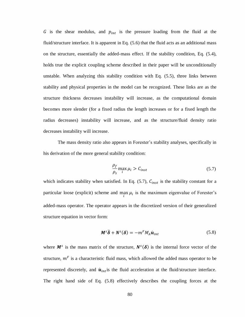
80
𝐺 is the shear modulus, and 𝑝𝑖𝑛𝑡 is the pressure loading from the fluid at the
fluid/structure interface. It is apparent in Eq. (5.6) that the fluid acts as an additional mass
on the structure, essentially the added-mass effect. If the stability condition, Eq. (5.4),
holds true the explicit coupling scheme described in their paper will be unconditionally
unstable. When analyzing this stability condition with Eq. (5.5), three links between
stability and physical properties in the model can be recognized. These links are as the
structure thickness decreases instability will increase, as the computational domain
becomes more slender (for a fixed radius the length increases or for a fixed length the
radius decreases) instability will increase, and as the structure/fluid density ratio
decreases instability will increase.
The mass density ratio also appears in Forester’s stability analyses, specifically in
his derivation of the more general stability condition:
𝜌𝑓𝜌𝑠max𝑖𝜇𝑖 > 𝐶𝑖𝑛𝑠𝑡 (5.7)
which indicates stability when satisfied. In Eq. (5.7), 𝐶𝑖𝑛𝑠𝑡 is the stability constant for a
particular loose (explicit) scheme and max𝑖 𝜇𝑖 is the maximum eigenvalue of Forester’s
added-mass operator. The operator appears in the discretized version of their generalized
structure equation in vector form:
𝑴𝑠�̈� + 𝑵𝑠(𝜹) = −𝑚𝐹𝑀𝐴�̇�𝑖𝑛𝑡 (5.8)
where 𝑴𝑠 is the mass matrix of the structure, 𝑵𝑠(𝜹) is the internal force vector of the
structure, 𝑚𝐹 is a characteristic fluid mass, which allowed the added mass operator to be
represented discretely, and �̇�𝑖𝑛𝑡is the fluid acceleration at the fluid/structure interface.
The right hand side of Eq. (5.8) effectively describes the coupling forces at the

81
fluid/structure interface. The constant, 𝐶𝑖𝑛𝑠𝑡 , has dependence on the time discretization of
the fluid domain and is typically ≤ 1 for most coupling schemes and the maximum
eigenvalue, max𝑖 𝜇𝑖 is typically >1, therefore the mass density ratio in Eq. (5.7) needs to
be ideally much <1 to maintain stability. The density ratio for the FSI models in this
thesis is 0.37, which is promising, however Forester suggests that the ratio should be very
small similar to the density ratio in aerodynamics problems [36].
To explore if the FSI models in this research follow the stability conditions
derived by Causin and Forester, a study to explore how the computational domain length,
i.e. slenderness ratio, and the structure/fluid density ratio affects stability was completed.
For the former, the length of the plate, 𝐿𝑝𝑙𝑎𝑡𝑒 , was varied from 0.4 m to 0.8 m at both 6
m/s and 7 m/s and for the latter, the fluid density was varied from 700 kg/m3 to 1400
kg/m3 at 6 m/s. Since increasing the fluid density will increase the pressure drop through
the model, the momentum at the inlet of the model will be fixed by adjusting the inlet
velocity. If the momentum were not fixed at the inlet, plate deflection would increase as
the fluid density increased, which would skew the study’s results since instability
increases with increasing plate deflection. Similar to the time step study, stability was
accessed by recording the deflection at “Point C” in Figure 5-4B.
The momentum at the inlet was fixed using the overall pressure drop through the
model. First, the analytic fluid model in Chapter 3.2 was used to find correlations
between pressure drop and velocity with various fluid densities. These results are shown
in Figure 5-5 with statistical power function curve fits at each fluid density. The curve fits
follow the general form:

82
𝑉𝑎𝑣𝑔,𝑐ℎ = 𝐽 ∗ ∆𝑃6 𝑚/𝑠
𝐾 (5.9)
where 𝐽 and 𝐾 are the constants in Table 5-1 for each respective fluid density, ∆𝑃6 𝑚/𝑠 is
the pressure drop at the nominal velocity and fluid density of 6 m/s and 997.6 kg/m3. This
pressure drop was calculated, using the analytic model, at the nominal velocity and fluid
density. This pressure drop was then plugged into Eq. (5.9) with the constants in Table
5-1 to find the average channel velocities. These results are shown in Table 5-1.
Figure 5-5. Trends for how the avg. ch. velocity varies as the pressure drop increases for
various fluid densities, trends were used to fix the momentum for the density ratio study.
Table 5-1 Density ratio, and average channel velocity results for fixed momentum analysis.
𝜌𝑓
(kg/m3)
𝜌𝑓
𝜌𝑠 𝑱 𝐾
𝑉𝑎𝑣𝑔,𝑐ℎ
(m/s)
700 0.259 0.0125 0.5675 7.00
800 0.296 0.0119 0.5661 6.60
900 0.333 0.0115 0.5649 6.25
997.6 0.370 0.0111 0.5639 6.00
1100 0.407 0.0108 0.5629 5.75
1200 0.444 0.0104 0.5627 5.55
1300 0.481 0.0101 0.562 5.33
1400 0.519 0.0099 0.5613 5.17

83
5.3.3 The Courant Number and a Stability Parameter
The explicit nature of the explicit (loose) coupling scheme detailed in Figure 5-3
will likely enforce an upper limit on the temporal step size due to the Courant-Freidrichs-
Lewy (CFL) condition:
𝐶𝐶𝐹𝐿 =
𝑉𝑎𝑣𝑔,𝑐ℎΔ𝑡
Δ𝑦 (5.10)
where 𝐶𝐶𝐹𝐿 is the Courant number, Δ𝑡 is the temporal step size, and Δy is the spatial step
size in the direction of the average channel velocity, 𝑉𝑎𝑣𝑔,𝑐ℎ. The Courant number only
takes into account the influence of the fluid on the FSI problem. Furthermore, the fluid
model utilizes an implicit scheme to solve for the fluid solution at each time step thus;
Courant numbers > 1 will likely allow the FSI problem to retain stability. Nonetheless,
the Courant number can be a rule of thumb for judging the numeric stability of an FSI
model.
Interestingly, the concept of a sonic CFL number can further explain the
destabilizing effect of an incompressible flow in FSI models. If the velocity in Eq. (5.10)
is replaced with the speed of sound through a fluid, the distance that sound or a
disturbance propagates through the fluid within a time step can be understood. For
compressible flows, the speed of sound is finite, thus a disturbance, i.e. from a structural
displacement, propagates through the fluid a finite distance, which is dependent on the
temporal step size. However, when a flow is considered incompressible disturbances in
the fluid at one point are instantly propagated through the entire fluid due to the infinite
sound speed in an incompressible fluid. Luckily, this does not make FSI models with
incompressible flows unconditionally unstable, but it does further explain their inherent
instability [49].

84
Explicitly coupled FSI models with incompressible flows interacting with thin
structures are also influenced by instabilities caused by physical quantities such as the:
The ratio of the fluid and structure densities
The slenderness of the geometry
The difference in the velocities through the channels flanking the plate
One can infer a stability parameter by creating a ratio of instability and stability inducing
terms such as:
𝐶𝑆 =
𝑖𝑛𝑠𝑡𝑎𝑏𝑖𝑙𝑖𝑦 𝑖𝑛𝑑𝑢𝑐𝑖𝑛𝑔 𝑡𝑒𝑟𝑚𝑠
𝑠𝑡𝑎𝑏𝑖𝑙𝑖𝑡𝑦 𝑖𝑛𝑑𝑢𝑐𝑖𝑛𝑔 𝑡𝑒𝑟𝑚𝑠=𝜌𝑓𝑉𝑎𝑣𝑔,𝑐ℎ (𝑏 − 𝑐) 𝐿𝑝𝑙𝑎𝑡𝑒
𝜌𝑠𝑎 (5.11)
This ratio closely resembles a Reynolds number without the fluid viscosity. Curiously,
the dimensions of this Eq. (5.11) resemble the kinematic viscosity of a fluid. Thus, it
would make sense to place the fluid viscosity into the denominator of Eq. (5.11), but
Forester mentions that increasing the fluid viscosity will decrease stability. Doing so
would skew the essence of Eq. (5.11) since fluid viscosity would be lumped with the
stability inducing terms. Forester also mentions that the stiffness of the plate, i.e. Young’s
modulus will increase stability as it increases, however this has a much smaller effect on
stability than for example the mass density ratio [37]. A similar conclusion was made
about the fluid viscosity. The difference in the thicknesses of the fluid channels, i.e. their
hydraulic diameters, was included in Eq. (5.11) to include the destabilizing effect of
offsetting the plate in the models.
In summary, the Courant number and the stability parameter, 𝐶𝑆, will be calculated
for all models completed in each of the empirical stability studies presented in the next
chapter. Optimistically, it will reveal a simple method for obtaining stable time
increments as well as provide a first order estimate of the stability of future models.

85
CHAPTER 6 - CODE COUPLING RESULTS
The previous three chapters outlined how the fluid flow around the plate is
modeled using the CFD code, Star-CCM+, how the plate deformation is modeled using
the FEA code, Abaqus, and how the two codes are coupled to build FSI models.
Specifically, the previous chapter described the difficulties of coupling codes with
staggered schemes as well as the advantages and disadvantages of two partitioned
schemes, namely the loose (explicit) and strong (semi-implicit) coupling methods. This
chapter provides the results the previous three chapters have been leading up to by
coupling the fluid and solid models in Chapter 3 and Chapter 4 using the loose (explicit)
coupling method from Chapter 5
6.1 Time Step Study Results
6.1.1 Initial Velocity Sweep Results
Starting at 3 m/s with a time step of 0.5 s the velocity was increased in 0.5 m/s
increments up until 5.5 m/s. The model took considerably longer to converge to a steady
state at 5.5 m/s than it did at 5 m/s. This is evident in Figure 6-1, at 5 m/s the model
reached a steady state after about 35 time steps whereas at 5.5 m/s the model took about
140 time steps to reach a steady state. Thus, to increase stability and decrease runtime at
6 m/s the time step was decreased to 0.1 s, which allowed the 6 m/s model to converge in
about 36 time steps. This also decreased simulation runtime by about one fourth when
compared to the runtime of the model at 5.5 m/s.
With a time step of 0.1 s at 6.5 m/s, the model was showing signs of instability
with large oscillations in deflection, thus to increase stability the time step was dropped
yet again, this time to 0.05 seconds. Figure 6-2 shows how, with a time step of 0.05 s, the

86
model converged within about 33 time steps and at 7 m/s the model converged in about
44 time steps (the plot was cutoff at 50 time steps to see more clearly how the models
react during early time steps). At 7.5 m/s, the time step was decreased to 0.0375 s and it
is evident that up until about 10 time steps the model is behaving chaotically, but the
model recovers from this chaotic behavior and converges in about 92 time steps.
Figure 6-1. Evolution of plate deflection at “Point C” from 3 to 6 m/s, solid line = 0.5 s time
step and dotted line = 0.1 s time step, zoom-in shows convergence behavior at low velocities.
The curves in Figure 6-3, for the models at 7.75 and 8 m/s, show an even greater
amount of chaotic behavior during the early time steps with plate movement between the
two fluid channels. A negative deflection value signifies the plate has moved into the
smaller 2.032 mm (80 mils) channel. It should be noted that the time step had to be
decreased to 0.0325 s and 0.03125 s at 7.75 m/s and 8 m/s, respectively. A model was
completed at 7.75 m/s because there was difficulty finding a time step that would allow a
model to converge at 8 m/s. The model at 7.75 m/s converged in about 180 time steps
whereas the model at 8 m/s converged in about 480 time steps.

87
Figure 6-2. Evolution of plate deflection at “Point C” from 6.5 to 7.5 m/s, solid line = 0.05 s
time step and dotted line = 0.0375 s time step.
Figure 6-3. Evolution of plate deflection at “Point C” at 7.75 and 8 m/s, solid line = 0.0325 s
time step and dotted line = 0.03125 s time step, zoom-in shows early chaotic behavior.

88
Table 6-1 details how much computer time, i.e. actual wall clock time, it took for
the models to converge to a steady state deflection at 2 through 8 m/s. It should be
mentioned that each of these models were ran on a 12-core workstation running at ~3.33
GHz with 96 GB of RAM. It is apparent that at velocities < 7 m/s the models converge
much faster than the model at 8 m/s. Also, keep in mind that at 1 thorough 5 m/s the time
step was 0.5 s and at 6 and 7 m/s the time step was set to 0.1 s and 0.05 s respectively.
Interestingly, if the time step is decreased to 0.031 s at 8 m/s the model converges in 32.2
hours instead of 43.1 hours with a time step of 0.3125 s.
Table 6-1 Wall clock time for the FSI models to converge to a steady state.
Velocity
(m/s) 2 3 4 5 6 7 8
Wall Clock
Time (hr) 0.85 0.91 1.01 2.34 4.74 3.45 43.1
Time Step
(s) 0.5 0.1 0.05 0.03125
It should be noted that during this initial velocity sweep from about 1 to 5 m/s
large time steps were adequate to allow the models to converge in a timely manner with
small oscillations that dissipated rather quickly. However, at all velocities > 5 m/s
continually decreasing time steps were preferred and sometimes required to attain
convergence, specifically at ≥ 7.5 m/s. Details about the stability of these models in the
context of their time step size is of interest, hence, the completion of the second velocity
sweep. Results of the second velocity sweep are included next, but first, details about
how the solutions of the models change as the velocity is increased is discussed.
Figure 6-4 shows how the maximum leading edge deflection behaved as the
average channel velocity was increased. The plot includes two power law curve fits
created using Microsoft Excel’s curve fitting tools. The first curve fit was completed up
to 5 m/s and it suggests that the deflection increases with nearly the square of flow

89
velocity. The second curve fit completed at the higher flow velocities suggests that
deflection trend increases more rapidly. While second order behavior with velocity is
consistent with linear drag analysis, non-linear behavior is an indicator of structural
changes in the system. Additionally, pressure drop through the model is highly dependent
on nonlinear terms such as the friction factor.
Figure 6-4. Maximum deflection at the leading edge of the plate vs. avg. ch. velocity.
Deflection contours from Abaqus at 5 m/s and 8 m/s are shown on the left and
right of Figure 6-5. At 5 m/s, the model shows one deflection peak at the leading edge
whereas at 8 m/s the model shows three distinct peaks; the first at the leading edge, the
second at about halfway from the leading edge, and the third towards the trailing edge of
the plate. This fundamentally different profile of deflection likely explains why at ~5.5
m/s, the curve fit in Figure 6-4 begins deviating from the data.
This change in plate profile can be seen more clearly in Figure 6-6. This figure
clearly shows how peaks downstream of the leading edge begin forming around 6 m/s,
and at 7 and 8 m/s, the peaks become more distinct. Interestingly, using Eq. (2.1), the
Miller critical velocity for a single plate is 6.14 m/s, which is curiously close to where the

90
deflection profile of the plate begins changing in the models. It should be noted, since
Miller assumed equal fluid channel thicknesses in his derivations, this calculation was
completed using the average channel thickness of 2.29 mm (90 mils).
Figure 6-5. Contours of deflection at 5 and 8 m/s, flow moves down in the –y direction.
Figure 6-6. Deflection profile extracted from the axial centerline of the plate in Abaqus.

91
6.1.2 Second Velocity Sweep Results
It is evident that stability has a high dependence on the size of the time step, thus
a second velocity sweep was completed. This time more emphasis was placed on how the
time step affects the model’s stability. The first sweep showed fast convergence with
relatively large time steps in the range of about 2 to 5 m/s, however decreasing the time
step appeared to allow the higher velocity models to converge more quickly and stay
more stable with less oscillatory behavior. Thus, at 2 and 5 m/s time steps above and
below 0.5 s were explored to see if the convergence speed and/or stability would vary.
Figure 6-7 shows how decreasing/increasing the time step at 2 m/s affects the
model’s convergence. With a time step of 0.05 or 0.075 s, the model diverged with
continually increasing oscillatory motion while a time step of 0.1 s allowed the model to
converge, thus stable models at 2 m/s are possible with ∆𝑡 ≥ 0.1 s. A time step of 2 s
allowed the model to converge slightly faster than the 0.5 and 0.1 s time steps.
Figure 6-7. Evolution of plate deflection at “Point C” at 2 m/s with different time step sizes
with zoom of stability with time steps of 0.5 and 2 s.

92
Figure 6-8 shows similar results as Figure 6-7 except the model’s velocity was at
5 m/s. A time step of 0.03 or 0.05 s caused the model to diverge in a similar way
as ∆𝑡 < 0.1 s affected the 2 m/s model, thus models at 5 m/s are stable at ∆𝑡 ≥ 0.075 s
since the 5 m/s model converged with a time step of 0.075 s. Increasing the time step
beyond 0.5 s caused the model to converge slower, this can be seen via the 2 s time step
response in Figure 6-8. The increased convergence time is likely caused by the model
overshooting steady state further as the time step increases. Interestingly, if these
responses are compared to control system behavior then the time step behaves in a similar
way as the gains in a proportional-integral-derivative (PID) controller, in particular the
proportional gain.
Figure 6-8. Evolution of plate deflection at “Point C” at 5 m/s with different time step sizes
with zoom of stability with time steps at 0.075, 0.5, and 2 s.
The explicit nature of the coupling algorithm in these models likely creates a CFL
condition or upper bound on the time step. However, increasing the time step to ≥ 2 s (at
these time increment the fluid/solid domains are likely solving to a steady state at each

93
time step) at 2 and 5 m/s does not cause the models to diverge or become unstable. This
suggests that the models, at relatively low velocities, do not have a CFL-like stability
condition. Conversely, there is a lower limit on the time step from 2 to 5 m/s.
It has been recommended in literature to decrease the time step as a way to
increase stability when coupling FSI models with loose (explicit) schemes (this is
particularly true for models that are strongly affected by the destabilizing added-mass
effect) [35]. However, as mentioned in Chapter 2.2, Forester et al. discovered in his
stability analyses on sequentially staggered or loose coupling schemes that stability may
increase with small time steps. The time step dependence appears when a derivation of
the added-mass operator (its maximum eigenvalue appears in Eq. (5.7)) is completed with
a discrete representation. However, the time step dependence only appears when the
derivation is completed on a stabilized fluid domain. If the derivation is carried out on an
unstabilized domain, the operator is only geometrically dependent, as in Causin et al.’s
derivations (Eq. (5.5)).
The maximum eigenvalue of the added-mass operator, derived discretely with a
stabilized fluid domain, increases with decreasing time step, thereby suggesting that a
lower bound on the time step exists for conditionally stable FSI models with
incompressible flows. This is apparent when examining Eq. (5.7), since the condition
moves closer to becoming satisfied as the maximum eigenvalue increases. This also
possibly explains why the models become unstable more quickly as the time step is
further decreased beyond a certain threshold. For example, the 0.05 s response at 2 m/s in
Figure 6-7 becomes unstable much quicker than the 0.075 s response; similarly, in Figure

94
6-8 the 0.03 s response at 5 m/s becomes unstable much quicker than the 0.075 s
response.
Forester et al. explored their stability conditions by allowing the bottom of the
classic lid driven cavity problem to structurally deform [36]. Using a stable model, they
investigated the influence of decreasing the time step on stability. Their results showed
instability increasing as the time step decreased ≤ 0.005 s. This can be seen in Figure 6-
9, a figure taken from their paper, by the zoomed in views showing instability when time
steps of 0.003 and 0.004 s were used. Furthermore, the 0.003 s time step showed
instability occurring significantly earlier than the 0.004 s time step. In summary,
Forester’s numerical observations are in excellent qualitative agreement with the results
shown in Figure 6-7 and Figure 6-8.
Figure 6-9. Response of a structurally deforming lid-driven cavity by Forester et al. showing
how decreasing the time step beyond a certain threshold causes instability [36].
The second velocity sweep was also completed at velocities > 5 m/s with more
refinement in the range of 5.25 to 6.5 m/s, since the deflection profile of the plate begins

95
to vary within this range. Furthermore, the Miller critical velocity for this geometry (6.14
m/s) also lies within this range. Figure 6-10 shows a summary of how the time step
affected the model’s stability from 5 to 8.25 m/s. The figure identifies three regions:
First, the green region, which signifies time steps that allowed the model to converge to a
consistent steady-state deflection. Second, the yellow region, which signifies time steps
that allowed the models to converge to steady-state deflections significantly different
from those in the green region and/or they converged to a stable plate oscillation.
Finally, the red region, which signifies time steps that caused the simulations to diverge
and/or crash. The range of stable time steps begins to narrow rather quickly as the flow
velocity is increased to greater than ~5.25 m/s. At velocities, around 7.5 and 8 m/s the
range of stable time increments that allow convergence are small and oscillations are
difficult to minimize as can be seen by the 7.75 and 8 m/s responses in Figure 6-3.
Figure 6-10. Map of stable, mildly unstable, and unstable time steps from 4.75 to 8.25 m/s.

96
Figure 6-11 shows how the models responded with time steps from the red,
yellow, and green regions at 6.5 m/s with the curve’s color corresponding to its respective
region in Figure 6-10. The solid green curve, the ∆𝑡 = 0.05 s response, shows the model
converging to a steady state in about 28 time steps. Conversely, the dotted red curve, the
∆𝑡 = 5 s response, shows the plate oscillating between the two fluid channels, hence the
negative (into the 2.03 mm (80 mils) and positive (into the 2.54 mm (100 mils))
deflection values. In a similar style, the solid yellow curve, the ∆𝑡 = 0.1 s response,
shows the plate oscillating, but only within the large channel. This model converged to a
steady-state deflection, whereas the ∆𝑡 = 5 s model diverged and crashed from a floating-
point exception in the turbulence model. However, the ∆𝑡 = 0.1 s model has a converged
deflection that is ~28% larger than the fully stable ∆𝑡 = 0.05 s model. Finally, the dashed
red curve, the ∆𝑡 = 0.03 s response, shows the model diverging rather quickly within 8
time steps caused by a negative fluid cell error triggered by crushed fluid cells.
Figure 6-11. Evolution of plate deflection at “Point C” with various time steps at 6.5 m/s.

97
As mentioned in Chapter 5.2.1, Star-CCM+’s built-in mesh morpher is utilized to
morph the fluid mesh around the deflected plates at each time step. The morpher tends to
morph cells around surfaces specified to deform differently than cells adjacent to rigid
surfaces. For example, in Figure 6-12A, the morpher appears to be trying to preserve the
thickness of the fluid cells near the plate (these surfaces were specified to deform),
whereas it appears to be thinning the cells near the rigid channel walls to accommodate
the increased thickness of the cells near the deforming surfaces. This distorted mesh
caused the fluid solution to diverge and cause a floating-point exception. It should be
noted, the mesh shown in Figure 6-12A was taken from a 6.5 m/s model, particularly the
model shown in Figure 6-11 with ∆𝑡 = 5 s. If the amplitude of the oscillations is large
enough, as in the ∆𝑡 = 0.03 s response in Figure 6-11, it can cause cells to crush at rigid
surfaces causing negative volume errors. This particular model’s mesh is shown in Figure
6-12B; notice the negative value for the colorbar’s lower bound.
Figure 6-12. Non-linear behavior of Star-CCM+’s built-in mesh morpher, contour is of cell
volume, both meshes are from 6.5 m/s models, A has ∆𝒕 = 𝟓𝒔 and B has ∆𝒕 = 𝟎.𝟎𝟑𝒔.

98
Luckily, it was discovered that Star-CCM+ includes an option to morph the mesh
from the initial, 𝑡 = 0 s mesh, which alleviates the morphing problems associated with
oscillatory behavior. It should be noted the actual fluid solver was not reset to t = 0 s after
each time step. Unfortunately, this option was discovered after the models in both
velocity sweep studies were completed, nonetheless the option was used in subsequent
studies in the following sections. However, this option does not solve the morphing
problem in the presence of large plate deflection that causes the plate and the channel
walls to nearly come in contact as shown in Figure 6-12B. Any morphing strategy would
likely lead to poor quality cells in this case. Luckily, there are alternatives to morphing
such as using overset meshing methods [41].
If the map in Figure 6-10 is instead plotted against the Courant number (Eq.
(5.10)) as shown in Figure 6-13 it becomes apparent that the lower limit has a nearly
constant Courant number of ~85, particularly at > 5 m/s. This is alarmingly high
considering the upper limit on the Courant number is 1 for 1D explicit schemes and this
limit only decreases as the number of spatial dimensions increase. However, the Courant
number only takes into account properties of the fluid partition of the FSI problem,
ignoring the structure partition. Furthermore, the fluid partition is solved implicitly and a
Courant number >1 is generally permitted with implicit schemes [50]. Implicit schemes
are not unconditionally stable especially when solving highly non-linear equations,
however they provide a much higher limit on the Courant number, hence the high values
for the Courant number in Figure 6-13. The limit is highly dependent on the problem and
the type of implicit scheme utilized. In summary, a more accurate FSI ‘Courant number’
correlation should take into account properties of the structure.

99
Figure 6-13. Map of the Courant number for models completed in the second velocity sweep.
It appears that the traditional Courant number can provide a first order estimate
for obtaining stable time step increments for the models presented thus far. At velocities
≤ 5 m/s, a Courant number of 125 appears to be stable and at > 5 m/s a Courant number
of 85 appears to be stable up until 8 m/s. Using these values for the Courant number and
rearranging Eq. (5.7) the time step, ∆𝑡, for obtaining a stable solution can be calculated
using:
∆𝑡 =
{
125∆𝑦𝑎𝑣𝑔𝑉𝑎𝑣𝑔,𝑐ℎ
, 2 𝑚/𝑠 ≤ 𝑉𝑎𝑣𝑔,𝑐ℎ ≤ 5𝑚 𝑠⁄
85∆𝑦𝑎𝑣𝑔𝑉𝑎𝑣𝑔,𝑐ℎ
, 5 𝑚/𝑠 < 𝑉𝑎𝑣𝑔,𝑐ℎ ≤ 8 𝑚/𝑠
(6.1)
where ∆𝑦𝑎𝑣𝑔 is the average length of the fluid cells through the channels in the direction
of flow. As can be seen in Figure 6-13, a Courant number much greater than 125 can be
utilized at velocities < 5 m/s. Conversely, at > 5 m/s, an upper limit appears and the
Courant number decreases as velocity increases. Therefore, a Courant number > 85 can
be used at some velocities around 5.5 and 6 m/s, but at > 7 m/s it is recommended to use

100
a Courant number of 85 since the upper and lower limits are very close to each other at >
7 m/s. Interestingly, Figure 6-6 shows that at velocities > 5 m/s the deflection profile of
the plate begins to significantly deviate from the profiles at < 5 m/s, which may be related
to the appearance of the upper limit as well as the rapid decrease in the Courant number
at > 5 m/s.
The second velocity sweep has shown that an upper and lower bound on the time
step size exists. The upper bound is likely a result of a stability condition emerging from
the explicit nature of the coupling, similar to the Courant-Freidrichs-Lewy (CFL)
condition. The lower bound, as explained earlier, likely develops from the added-mass
effect that appears in sequentially staggered methods like the explicit (loose) coupling
scheme utilized in these models. The two restrictions appear to meet at 8 m/s and they
possibly begin to overlap at > 8 m/s thus, creating an empty set of stable time step
increments at > 8 m/s. It should be noted, the restrictions found during this time step
study are dependent on the spatial meshes, geometry, and physics used in the models.
6.2 Results of Slenderness and Mass Density Ratio Studies
6.2.1 Slenderness Ratio Results
According to Causin et al.’s stability analyses, stability is dependent on the length
of the computational domain thus, the length of the plate, 𝐿𝑝𝑙𝑎𝑡𝑒 , was varied to explore if
the models behave as predicted by Causin. It should be noted, for all models at 6 m/s the
time step was held constant at 0.05 s and the number of cells was linearly increased along
the plate as its length was extended in both the fluid and plate meshes. Furthermore, the
fluid mesh in all models was morphed from 𝑡 = 0 s at each time step.

101
Figure 6-14 shows how the model’s solutions evolved as the plate length
increased from 0.4 to 0.8 m at 6 m/s. It is apparent when the plate is 0.8 m long the model
becomes unstable with rapidly growing plate oscillation. This eventually caused the 2.03
mm (80 mils) fluid channel to become nearly closed-off. With the plate approaching the
channel wall so closely, the morpher was forced to nearly crush the cells perpendicular to
the plate as similarly shown in Figure 6-12B. These poor quality cells led to a floating-
point exception that originated in the turbulence model.
Interestingly, when then models converged from 0.4 to 0.75 m the maximum plate
deflection did not increase. Figure 6-15 also shows how the general shape of the axial
plate deflection profiles stayed constant as the length increased. The profiles seem to only
elongate through the mid-section of the plate as its length increases. Furthermore, the
Figure 6-14. Evolution of plate deflection at “Point C” with various plate lengths at 6 m/s with
zoom-in of the stable plate lengths.

102
differential pressure (calculated by subtracting the 2.54 mm (100 mils) channel’s pressure
from the 2.03 mm (80 mils) channel’s pressure at various axial locations along the plate),
shown in Figure 6-15, followed a similar trend as the plate deflection. However, the
overall pressure drop through the models did increase as the plate was lengthened due to
the higher frictional pressure drops through the longer channels.
To further explore why plate deflection stays constant as its length is increased a
fluid flow study was conducted in Star-CCM+ with a rigid plate that was not allowed to
deform. In this study, the differential pressure on the plate was extracted to see if it varied
as the plate was lengthened. Figure 6-16 shows how the fluid flow around longer plates
has a higher differential pressure when the plate is held rigid. This is counterintuitive
since when the plate is allowed to deform it settles into a general plate profile regardless
of its length. However, the deflection solution after the first time step in the FSI models
increased as the plate was lengthened. This can be seen in Figure 6-14’s zoom-in view by
Figure 6-15. Axial plate deflection (blue curves) and differential pressure (red curves) on the
plate for each plate length at 6 m/s.

103
the dark blue curve (0.75 m) being above the yellow curve (0.4 m) at t = 0.05 s. Thus, the
physics of the interaction between the fluid and the plate must be coaxing the plate to
deform into the general plate profile shown in Figure 6-15.
The plate length was also varied from 0.4 to 0.75 m at 7 m/s and in a similar
manner as the 6 m/s models, stability declined as the plates became longer. This is
apparent if the oscillatory behavior in Figure 6-17 around 0.1 to 0.3 s is examined. The
model with a 0.75 m plate diverged with continually increasing plate oscillation between
the fluid channels. Like the 0.8 m plate at 6 m/s, this eventually led to a floating-point
exception in the turbulence model. It should be noted, the time step was decreased to 0.04
s for all the 7 m/s models in this study.
Similar to the models at 6 m/s, Figure 6-17 appears to indicate the 0.4 through 0.7
m plates converging to about the same steady-state deflection, however if the plate
profiles in Figure 6-18 are examined closely, one can see that the 0.4 m plate deflected
slightly more than the longer plates. This is likely because the deflection peak at the
leading edge runs into where the second deflection peak would normally appear at about
Figure 6-16. Differential pressure on the plate at 6 m/s, plate deformation was not allowed (the
plate was held rigid).

104
0.35 m from the trailing edge. The differential pressure profiles for the stable models at 7
m/s are also included in Figure 6-18.
Figure 6-17. Evolution of plate deflection at “Point C” with various plate lengths at 7 m/s.
Figure 6-18. Axial plate deflection (blue curves) and differential pressure (red curves) on the
plate at 7 m/s.

105
To summarize, this study has shown how the length of the plate, with all other
parameters held constant, has a direct effect on stability. This relationship has also been
seen by Nobile and Causin et al. who showed that stability is directly related to the
geometry’s slenderness ratio using simplified analytic models [35].
6.2.2 Mass Density Ratio Study Results
Causin and Forester both found that as the structure density decreases or as the
fluid/structure density ratio, 𝜌𝑓 𝜌𝑠⁄ , increases loosely coupled models will become more
unstable [35]. Thus, using the average channel velocities in Table 5-1, which were
calculated using the curve fits in Figure 5-5, the momentum was fixed at the inlet so plate
deflection would not increase as a result of a higher fluid density. It was found that the
models become more unstable as the fluid density was increased. However, the models
remained stable until the fluid density was set to 1400 kg/m3, which caused the model to
diverge with rapidly growing instabilities as seen in Figure 6-19. The instability caused
the model to nearly close off the 2.54 mm (100 mils) fluid channel, which created a
floating-point exception in the turbulence model.
The five stable models in Figure 6-19 converged to a common plate deflection
that varied < 3.8%. It should be noted, all other parameters in these models, excluding
the inlet velocity and fluid density, were held constant including the time step, which was
set to 0.05 s. In summary, the density ratio, 𝜌𝑓 𝜌𝑠⁄ , is directly related to the stability of the
models and an upper limit on the ratio exists. Using this upper limit the stability number,
𝐶𝑆𝑡𝑎𝑏𝑖𝑙𝑖𝑡𝑦 , was calculated to be 27,466. Interestingly, this value matches nearly exactly
with the stability number calculated in the slenderness ratio study at 6 m/s.

106
The results of the stability studies in this section have confirmed some of the
theories developed by Causin and Forester. This includes demonstrating that the models
in this thesis follow Causin’s theory about how stability and the length of the
computational domain are related. The fact that the two are related is quite astonishing
especially considering the stability increases independently of the model’s steady-state
plate deflection. Clearly, this is a result of the physics behind how the fluid interacts with
the plate since solving the fluid and plate problems independently indicates that plate
deflection would increase as the length is increased. Furthermore, the dependence of the
density ratio on stability, included in both Causin’s and Forester’s theories, was also
demonstrated using the models in this thesis. Again, the plate deflection did not increase
with larger density ratios, but unlike in the plate length study the inlet momentum had to
be fixed otherwise it would have.
Figure 6-19. Evolution of plate deflection at “Point C” with various fluid densities.

107
6.3 Discussion of a Stability Parameter
In the previous chapter, a stability parameter, 𝐶𝑠, was hypothesized, which was
based on studies completed in literature as well as other properties in the models that will
influence stability such as fluid velocity. The parameter is a ratio of instability/stability
inducing properties of the models and includes the fluid/structure mass density ratio, the
slenderness ratio of the plate, the fluid velocity, and the difference in the thickness of the
channels, i.e. the hydraulic diameters. The goal of this discussion is to present a first
order method for obtaining a stable time increment based on the physical properties of the
model as well as, to an extent, the spatial mesh size.
First, a map of the stability parameter, 𝐶𝑠, was created by varying the velocity and
the length of the plate since both of these properties have been explored (Figure 6-20).
On Figure 6-20’s map, two black isolines are shown where 𝐶𝑠 = 0.9 and 𝐶𝑠 = 1.0. The
three unstable models fall within/on these isolines, however; stable models also fall
within these isolines suggesting that between them models may be stable or unstable.
This region can be thought of as being similar to a transitional flow where the flow can
be laminar or turbulent or in this case stable or unstable. Within the isolines or the yellow
to red region, the limits on the Courant number will be strict and the time step increment
should therefore be calculated using the second equation in Eq. (6.1), particularly when
the velocity is > 5 m/s. For models where 𝐶𝑠 is less than 0.9 the restriction on the Courant
number is more lax and it is suggested to use the first equation in Eq. (6.1) to find a stable
time increment, particularly when the velocity < 5 m/s.

108
The map in Figure 6-21 is similar to Figure 6-20 except plate length is replaced
with fluid density and the models completed during the mass density ratio study are
included. The same isolines from Figure 6-20 are also included; however, the unstable
model with a fluid density of 1,400 kg/m3 lies outside the region bounded by these
isolines. During the density ratio study, the velocity had to be adjusted as the fluid
density was varied to keep plate deflection constant and with a fluid density of 1,400
kg/m3, the velocity was set to ~5 m/s. This corresponds to a Courant number of ~86,
which violates Eq. (6.1) for velocities at 5 m/s. The model’s large mass density ratio
compounded with the small Courant number at 5 m/s likely explains why this model went
unstable. This particular model shows how Eq. (6.1) and Eq. (5.11) need to be used
together to judge the stability of a model.
Figure 6-20. Map of Cs as velocity and plate length vary with FSI model results overlaid.

109
A simple method for judging the stability of a model is to first calculate the
stability parameter, 𝐶𝑠 using Eq. (5.11). If 𝐶𝑠 is < 0.9, the model will most likely be stable
if a stable time increment is calculated using Eq. (6.1), which is based on the velocity and
the spatial mesh size in the flow direction. In summary, Eqs. (5.11) and (6.1) can be
utilized as a first order estimate of a model’s stability before the model is started.
The spatial mesh sizes were kept constant for all the models presented thus far,
therefore an understanding of how the mesh size affects stability is not understood. A
better understanding of how the spatial mesh size affects stability will likely reveal a
better way for calculating stable time increments. Currently, a Courant number
correlation, Eq. (6.1), has been suggested for use to find stable time increments however,
the Courant number does not take into account properties of the structure. This is likely
Figure 6-21. Map of Cs as velocity and fluid density vary with FSI model results overlaid.

110
the reason why the Courant number for the stable models presented thus far have rather
high values in comparison to the suggested Courant number of < 1.
This method of using Eqs. (5.11) and (6.1) to judge if a model will be stable is
not perfect and violations may be found. Other parameters in the models such as fluid
viscosity and Young’s modulus likely have an influence on stability and are not included
in either equation. However, Forester suggested that fluid viscosity and plate stiffness do
not have as large as an effect on stability as other properties such as the time step size and
the mass density ratio. For future studies, it is suggested to explore the spatial mesh sizes,
the plate stiffness, the fluid viscosity, the plate width, and other properties in the models
that may affect stability. Using the data collected during these studies, a more refined
stability parameter can be found, however the non-linearity of the fluid and structure
equations will likely make it impossible to find a method that will be perfect.

111
CHAPTER 7 - EXPERIMENT SETUP AND COMPARISON TO FSI MODELS
This chapter describes the experimental tools currently being used to benchmark
the FSI models. The hydro-mechanical flow loop is described in detail as well as how the
measurements were taken. The measurements are then compared to the solutions of the
FSI models presented in Chapter 6. A new laser positioning system is then presented with
details of the design as well as a discussion of how the design will improve future laser
measurements. Finally, details on how custom parts for the new positioning system were
manufactured using additive techniques are described.
7.1 Experimental Setup (University of Missouri Flow Loop)
The experimental setup presented in this chapter was designed, built, and rebuilt
many times as a collaborative effort between many researchers in the TherMec research
group. These researchers include Dr. Kyler K. Turner, John C. Kennedy, Philip F.
Makarewicz, and Robert Slater. The current flow loop design, shown in Figure 7-1, was
designed to accommodate a variety of modular test sections. The loop has the ability to
control the downward flow through the “test section area” shown in Figure 7-1 using two
flow configurations. This allows the pressure within a test section to be either above or
below ambient pressure.
The flow loop is driven with a Sta-Rite Max-E-Pro P6E6F-207L 230 V pump. To
control the single speed pump a pneumatic control valve is used. The “flow control
valve” is located on the bypass line of the loop. When the valve is fully open, the flow is
minimized through the test section and when it is closed, the maximum amount of flow is
forced through the test section. The flow control valve does not vary the flow linearly.
Figure 7-2 shows how the flow rate varies as the control valve is closed [48]. The loop is

112
also equipped with a water filtration system, which includes 3 micron and 25 micron
filters. To control test section corrosion, the water is also treated with an acid (currently
vinegar) to keep the pH to ~5.5. A more detailed description of the flow loop and its
capabilities can be found in the flow loop’s equipment specifications documentation [48].
Figure 7-1. University of Missouri Hydro-Mechanical Flow Loop.
Figure 7-2. System flow rate calibration curve. Note: System is in (+) pressure mode.

113
7.1.1 Flat Plate Test Section
As mentioned earlier the flow loop was specifically designed to accommodate a
variety of different test section designs. One of those test sections is shown in Figure 7-3
with dimensions in Table 7-1. This test section’s focus is to measure the change in the
thickness of two flow channels (the thicknesses of b and c in Figure 7-3) flanking the
nominally flat aluminum plate, which deforms as the flow rate is increased. Two laser
displacement sensors, Keyence LK-G152s, are used to take high speed, high accuracy
measurements of the change in these channel thicknesses as the flow deforms the
aluminum plate. The test section is also equipped with pressure taps for taking static
pressure measurements with an array of Omega PX26 pressure transducers. The loop is
equipped with a paddle wheel flow meter, shown in Figure 7-1, so the flow rate can be
monitored at all times during the experiment.
Figure 7-3. Flat plate test section diagram and photo.

114
Table 7-1. Nominal dimensions of the test section assembly.
𝒂 1.02 mm (40 mils)
𝒃 2.54 mm (100 mils)
𝒄 2.03 mm (80 mils)
𝒅 (𝒊𝒏𝒕𝒐 𝒑𝒂𝒈𝒆) 110.3 mm (4.342”)
𝑳𝒊𝒏𝒍𝒆𝒕 190.5 mm (7.5”)
𝑳𝒑𝒍𝒂𝒕𝒆 647.7 mm (25.5”)
𝑳𝒐𝒖𝒕𝒍𝒆𝒕 76.20 mm (3”)
7.1.2 Previous Laser Positioning Systems and Channel Mapping Procedure
The test section shown in Figure 7-3 was assembled with nominal channel gap
thicknesses of 2.03 mm (80 mils) and 2.54 mm (100 mils). However, realistically these
values will vary in both the flow direction and along the width of the plate. To
characterize this variance, a mapping of the channel gaps was completed by taking laser
measurements at various locations on the test section before the flow experiments were
started. Two different positioning systems were utilized for the channel mapping and the
flow experiments.
The left photo in Figure 7-4 shows the laser positioning system used to map the
channel gaps and the right photo shows the system used during the flow experiments. The
system used during channel mapping automated laser motion along the width of the plate,
but the axial motion (direction of flow) was moved by hand with the red scissor jacks in
Figure 7-4. The system used during the flow experiments did not have automated laser
motion in any direction. However, the structure for the flow experiments was stiffer and
allowed the laser’s position to be more stable than the cantilevered design used during the
channel mapping. Furthermore, the support structure of the flow experiments system
provided an excellent foundation for a new positioning system to be designed and built

115
for future channel mapping studies and flow experiments. Details about the design of the
new positioning system, and how it was built are included later.
Figure 7-4. Laser positioning system for channel mapping (left photo) and flow experiments
(right photo) [49].
To quantify the variance in the channel gap thicknesses, the lasers were
positioned at the 120 locations shown in Figure 7-5. At each location, 30 samples were
taken. Once all 120 locations were visited once, this measurement process was then
repeated eight more times. Replicating this process nine times will help reveal the
repeatability of the positioning system to return to a given location.

116
Figure 7-5. Measurement locations for fluid channel mapping [49].
7.1.3 Flow Experiment Procedure
A brief overview of the procedure used during the flow experiment is: [49].
Position the Lasers: Position the lasers at the desired axial and horizontal
location. Rotate the lasers down 8.5° from perpendicular to the test section.
Collect calibration Data: Details in the document TDR-MU-201404-001C [49].
Bleed the Pressure Lines: With the water flowing at the lowest flow rate, bleed
air out of all pressure lines.
Begin Data Collection: Begin with the lowest flow rate, collect data for
approximately 30 seconds at a sampling frequency of 1650 Hz, and then move on
to the next flow rate.
Repeat at Next Laser Position: Repeat the process until data at all laser positions
has been recorded.

117
The lasers were positioned at the seven axial (direction of flow) locations shown in
Figure 7-3 and detailed in Table 7-2. At each of these positions, the flow velocity was
varied from 2 to 9 m/s with extra refinement in the 5 to 6 m/s range. It should be noted
that the channel gap measurements along the axial length of the plate were not taken
during a single flow test, therefore the axial profiles of the plate position should be used
tentatively. The static pressure at the eighteen pressure taps (spaced 6.47 cm (2.55”)
apart) shown in Figure 7-3 were continuously monitored during flow testing. Detailed
specifics of the measurements and the procedure are included in [49].
Table 7-2. Axial laser locations during the experiment (distances are from the plate's trailing
edge)
Location Axial Location
(from Plate Trailing Edge)
𝑨 12.7 mm (0.500”)
𝑩 152.4 mm (6.000”)
𝑽 226.7 mm (8.925”)
𝑫 290.5 mm (11.438”)
𝑬 474.3 mm (18.675”)
𝑭 550.5 mm (21.675”)
𝑮 635.0 mm (25.000”)
7.2 Experiment Results and Comparison to FSI Models
7.2.1 Channel Mapping Results
It should be noted, hereafter “small channel” will refer to the ideally 2.03 mm (80
mils) channel and “large channel” will refer to the ideally 2.54 mm (100 mils) channel.
The measured channel gap at each location is shown in Figure 7-6. All nine trials are
included, thus Figure 7-6 shows 1,080 data points. The x-axis corresponds to the 120
locations shown in Figure 7-5, therefore the right side of the plot shows the horizontal
sweeps on the top half of the plate and the left side shows the sweeps from the bottom

118
half of the plate. The gap thicknesses vary > 0.3 mm (~12 mils) from trial to trial at some
locations. This can be more easily seen by the standard deviations in Figure 7-7. For both
channels, the standard deviations are mostly banded around 0.05 mm (~2 mils) with
outliers as far as 0.10 mm (~4 mils).
If it is assumed these measurements follow a normal distribution and a 95%
confidence interval is taken, the true value of the gap thickness is within a range of
±0.065 mm (±2.6 mils). However, it is desired for uncertainty to be < 0.025 mm (1 mil).
Thus, it is apparent that the laser positioning system shown on the left side of Figure 7-4
is not adequate if uncertainty is desired to be < 0.025 mm (1 mil).
Figure 7-6. Measurements for all nine sweeps through the 120 location measurement process.

119
Figure 7-7. Standard deviation of the nine trials at each measurement location.
The channel maps in Figure 7-8 were created using the average of the nine trials
with a cubic interpolation between measurements. It also includes a map of the difference
between the two channels (large channel – small channel), also created using a cubic
interpolation method. When the channel difference is positive, the large channel is bigger
than the small channel and when it is negative, the inverse it true. The channel difference
is mostly positive, but is slightly negative from ~127 mm (5”) to ~254 mm (10”) from the
trailing edge of the plate. To see this more clearly, Figure 7-9 shows the axial profile of
the channel gaps as well as the channel difference at approximately the centerline of the
plate without the cubic interpolation between the measurements.
It is evident that a more robust laser positioning system is needed. A system with
automation axially would provide a simple and efficient way to increase the axial
measurement density, while concurrently decreasing the standard deviation between trials
since positioning would not have to be completed by hand.

120
Figure 7-8. Average of the nine trials at each measurement location for both channels as well
as the difference between Channel 1 and Channel 2 [49].
Figure 7-9. Large and small channel gap thicknesses and channel difference at approximately
the centerline of the plate.

121
7.2.2 Flow Experiment Results and Comparison to Models
The FSI models must be validated against an experiment; therefore, the flow loop
and test section were utilized with the experimental procedure to obtain usable data for
benchmarking. The curves in Figure 7-10 compare the change in channel gap over a
range of flow velocities from both the experiment and the FSI models. Square points
connected with dashed lines represent experimental data while series with solid curves
represent plate profiles from the models. Furthermore, positive values indicate the plate
has deflected into the large channel whereas negative values indicate the plate has
deflected into the small channel.
Figure 7-10. Comparison of the experiment with the models showing the change in channel
gap thickness, points connected with dashed lines are experimental data and solid lines are
solutions from the models.

122
In the experiment, the plate generally moves into the large channel, however once
the flow velocity increases to ~6.8 m/s, the plate snaps into the small channel. This
snapping behavior was not seen in the models. Therefore, an attempt will be made to
determine the cause of the experiment/model discrepancy seen in Figure 7-10. First, to
provide a clearer picture of Figure 7-10, a comparison at each velocity is provided in
Figure 7-11 through Figure 7-17 using data from both lasers. However, keep in mind, the
experimental measurements for a given flow velocity were collected at different points in
time such that they cannot conclusively be interpreted as the axial profile of the plate for
that flow velocity. The experiment velocity in each figure is an average of the measured
velocities when each individual channel gap measurement was taken. These 7 velocities
are split into three sets: The low range in Figure 7-11 through Figure 7-13, the middle
range in Figure 7-14 and Figure 7-15, and the high range in Figure 7-16 and Figure 7-17.
Each respective set is plotted with fixed axis limits for comparison purposes.
Figure 7-11. Comparison of the model (solid line) to the experiment (dashed lines) at ~2.06
m/s.

123
Figure 7-12. Comparison of the model (solid lines) to the experiment (dashed lines) at ~2.77
m/s.
Figure 7-13. Comparison of the model (solid lines) to the experiment (dashed lines) at ~3.46
m/s.

124
Figure 7-14. Comparison of the model (solid lines) to the experiment (dashed lines) at ~4.55
m/s.
Figure 7-15. Comparison of the model (solid line) to the experiment (dashed lines) at ~5.14
m/s.

125
Figure 7-16. Comparison of the model (solid lines) to the experiment (dashed lines) at ~6.8
m/s.
Figure 7-17. Comparison of the model (solid lines) to the experiment (dashed lines) at ~7.75
m/s.

126
The majority of the data points in Figure 7-11 through Figure 7-13 lie in the small
channel despite the fact that the models deflected exclusively into the large channel.
However, if this fact is ignored, the trend of the data from “Laser B” near the leading and
trailing edges follows the models for the most part. Data from both lasers shows the
leading edge moving further into the large channel as the velocity increased. Through the
mid-section of the plate, from ~0.3 to ~0.5 m, “Laser B” shows the plate ‘bulging’ into
the small channel, which never appears in the models at any velocity.
At ~4.55 and ~5.14 m/s, the experiment shows nearly the entire plate deflecting
into the large channel, which is conducive to the model’s behavior. It appears that as the
velocity is increased in the experiment the plate gradually moves from the small channel
to the large channel. Thus, at ~5.14 m/s, Figure 7-15 clearly shows the closest matching
of all 7 comparisons to the experiment. This is likely a result of both lasers showing 6 out
of 7 locations deflecting into the large channel at ~5.14 m/s, furthermore the lone outlier
only deflected ~0.05 mm (1.97 mils) into the small channel.
The next three velocities completed in the experiment at ~5.47, ~5.66, and ~5.85
m/s are included in Appendix 1. These were not included because data points near the
leading edge had ‘snapped’ into the small channel while points near the trailing edge had
not ‘snapped’ yet. This is a result of the plate ‘snapping’ at slightly different velocities
during the experiment. Thus, the data could not be interpreted as a profile for comparing
to the models. More information about the ‘snapping’ phenomenon is included in [49].
The final two velocities, at ~6.79 and ~7.75 m/s, are post-snap velocities, thus the
experiment shows the plate deflecting completely into the small channel. Furthermore,
the magnitude of the deflection in the experiment is more than double the deflection

127
predicted by the model in most locations. This atypical behavior observed in the
experiment is counter to all numeric and analytic calculations that have been made, and is
a strong indicator that for particularly high flow velocities additional features need to be
added to the model for more accurate predictions.
The shape and magnitude of deflection is highly dependent on the initial (no-
flow) geometry of the flow channels, and this is likely the cause of the difference
between the plate deflections measured and predicted in the experiment and the models.
Figure 7-18 compares the channel difference in the models, which was constant due to
assuming uniform flow channels, the channel mapping, and the flow experiments. The
green points were taken just before the flow experiments were started, which allowed
deflection values to be calculated. It is quite evident that the large discrepancy between
the models and the experiment is a result of the drastic difference between the geometry
assumed in the models and the actual geometry measured in the experiment.
Figure 7-18. Comparison of the channel difference assumed in the models, measured during
the channel mapping, and measured just before the flow experiments.

128
There are likely many sources causing the non-uniformity of flow channels in the
experiment including:
The plate is only nominally flat and might have a slight curvature.
o The magnitude of this plate curvature might be amplified when the
test section is bolted together.
The plate and/or spacers, which space the plate from the Plexi-glass panels
to create the flow channels, might not be uniformly thick.
The Plexi-glass panels might have become distorted due to water
absorption.
o Zabriskie found that his Plexi-glass plates were swelling after < 4
hours of water exposure, which caused them to buckle when they
were clamped in his experimental test section [27].
Any number of these sources might be causing non-uniformity in the flow channels of the
test section. Thus, a new and more robust laser positioning system needs to be developed.
A new system will aid in obtaining a denser mapping of these non-uniformities seen in
Figure 7-8. In particular, automated movement in the axial flow direction will allow a
finer axial profile of the channel gaps to be obtained. These finer mappings can be used
in future FSI models to help facilitate the merging of the model’s solution to the
experiment’s data.

129
7.3 Laser Positioning System
The laser positioning system used to complete the fluid channel gap mapping
discussed earlier was shown to be inadequate with measurement uncertainties
approximately ±0.065 mm (±2.6 mils). In an attempt to decrease the error associated with
the previous system a new system that automates positioning in both the X and Y
directions using stepper motors was designed and built. In addition, since the new system
has the ability to be completely automated the density of the measurement grid in Figure
7-5 can be increased.
In summary the new positioning system should have the ability to automatically
position the lasers axially (Y direction) and laterally (X direction) while also being able
to rotate the angle of the lasers. It was also desired to keep the pre-existing structure
(right photo in Figure 7-4) used in the flow experiments since this structure is already
very rigid and it holds the test section very well.
7.3.1 New Positioning System Design
The new positioning system was designed in the commercial 3D CAD program
SolidWorks. A rendering of the full design is shown in Figure 7-19 with some labels of
the major components of the design. Figure 7-20 shows a zoomed in view of the new
system. To control axial positioning, two high torque stepper motors simultaneously
rotate two lead screws that vertically move the horizontal rail in Figure 7-20. Lead screws
were used over ball screws since lead screws are more robust for vertical motion and they
are considerably less costly. Furthermore, ball screws require braking systems especially
in vertical applications [50]. The horizontal rail is attached to the lead screws with lead
screw travel nuts and a custom designed bracket. Two sets of wheels (sourced from the

130
supplier of the aluminum extrusions) were added for stabilizing and providing smooth
vertical motion of the horizontal rail. The two axial stepper motors are mounted to the
existing structure with custom brackets (top two green parts in Figure 7-20). To transmit
the motion of the axial steppers to the lead screws, motor couplers were used and thrust
bearings were added to help bear the load of the lead screws and the horizontal rail. The
two green parts below the thrust bearings were designed to clamp a set of ball bearings
for holding the lead screws in position. Another set of these mounts are at the bottom of
the lead screws as shown on the bottom of Figure 7-19.
The horizontal rail has a high precision linear guide rail attached to it for
controlling lateral motion of the laser. A timing belt is used to move the linear rail’s
carriage (red, green, and silver part below the laser in Figure 7-20) using a stepper motor.
A part was then designed to attach the carriage of the linear rail to the stepper motor used
to rotate the angle of the laser. The final part of the horizontal rail is a part that was
designed to hold a couple of flanged bearings that create a pulley for the timing belt. An
identical but mirrored system will be utilized for the laser on the opposite side of the test
section. This allows each laser to have completely independent motion, an attribute that
the previous positioning system, left photo of Figure 7-4, did not have.
Overall, this new positioning system design includes five different parts that must
be manufactured. In total, twenty parts must be manufactured when both positioning
systems, one for each laser, are considered. These parts could be manufactured with stock
material, such as aluminum, using traditional subtractive processes or they could be
manufactured using additive techniques such as fused deposition modeling (FDM).

131
Figure 7-19. Full rendering of the new laser positioning system.
Figure 7-20. Detailed view of the horizontal rail.

132
7.3.2 Manufacturing Processes for Custom Parts
The green parts shown in Figure 7-19 and Figure 7-20 were specifically designed
for the new positioning system. Therefore, they must be manufactured. Both traditional
subtractive machining processes and newer additive manufacturing techniques (rapid
prototyping) were considered to fabricate the parts. Traditional machining techniques
utilize stock materials such as Al 6061-T6 and rapid prototyping techniques utilize
thermoplastic filament such as polylactic acid (PLA). To compare the two techniques a
cost analysis for the materials used in each process was completed.
Table 7-3 details the material costs to traditionally machine the parts and Table
7-4 details the material costs to rapid prototype the parts. From the material cost
perspective, traditional machining would cost more than four times that of using rapid
prototyping. Furthermore, the cost of machine shop time would have to be added to the
overall cost if the parts were machined. This cost would likely be substantial since many
hours would have to be spent in the machine shop.
Table 7-3. Material cost for traditional manufacturing.
Traditional Manufacturing Material Costs
Part Quantity Material Raw Material Size Cost
Lead Screw Bearing Mount
8 Aluminum 38.1 x 50.8 x 1,828 mm
(1.5" x 2" x 72") $107.42
Stepper Motor Bracket
4 Aluminum 50.8 x 50.8 x 610 mm
(2" x 2" x 24") $47.12
Rail Bracket 4 Aluminum 203.2 x 203.2 x 4.83 mm
(8" x 8" x 0.19") $18.19
Laser Bracket 2 Aluminum 63.5 x 63.5 x 152 mm
(2.5" x 2.5" x 6") $27.25
Pulley Bracket 2 Aluminum Use Excess Material from Bearing Mount
-

133
Table 7-4. Material cost for additive manufacturing, cost per cm3 is ~$0.05.
Rapid Prototyping Material Cost
Part Quantity Material Sliced Volume
(cm3) Total Volume
(cm3) Cost
Lead Screw Bearing Mount
8 PLA ~75 600 $30.00
Stepper Motor Bracket
4 PLA ~45 180 $9.00
Rail Bracket 4 PLA ~17 68 $1.90
Laser Bracket 2 PLA ~28 56 $2.80
Pulley Bracket 2 PLA ~13 26 $1.30
Another perspective to compare is the strength of the two materials, Al 6061-T6
and PLA. This comparison is not as transparent as the cost analysis since the strength of
parts manufactured using FDM is slightly ambiguous due to the parts being created layer
by layer. The height of these layers and the temperature the parts are manufactured are
just a few of the factors that affect the strength of the finished parts. As a simple
comparison, the modulus of elasticity as well as the tensile strength is compared in Table
7-5. It is quite apparent that using aluminum would provide a much stronger part, but at a
much higher material and manufacturing cost.
Table 7-5. Material property comparison of Al 6061-T6 and polylactic Acid [43, 51].
Poly(lactic) Acid Al 6061-T6
Density 1.24 g/cm3 2.7 g/cm
3
Young's Modulus 2.02 to 3.54 GPa 68.9 GPa
Tensile Yield Strength 48.3 to 56.2 MPa 276 MPa
Ultimate Tensile Strength 60.95 to 65.5 MPa 310 MPa
To assure using PLA would not yield under the static loads in the new system a
simple beam analysis was completed. The lead screw bearing mount will be under the
highest stress thus this part will be analyzed to assure it will not yield. The bearing mount
was simplified as shown in Figure 7-21 so a simple beam theory calculation could be
utilized to estimate the deflection when the mount is rapid prototyped with PLA. The

134
bearing mount was simplified as a cantilevered beam with a load applied a certain
distance from the free end as shown in Figure 7-21. Equation (7.1) describes the
maximum deflection (at the end of the beam) for the geometry shown in Figure 7-21
𝛿𝑚𝑎𝑥 = −
𝐹𝑙3
6𝐸𝐼(2𝑙3 − 3𝑙2𝑎 + 𝑎3) (7.1)
𝐼 =
𝑏ℎ3
12 (7.2)
where l is the length of the beam, F is the load, E is Young’s modulus, I is the area
moment of inertia, and a is the distance from the free end to the load F [44]. For a
rectangular beam, I is found using Eq. (7.2). The bending moment and therefore the
normal stress are both maximum at the fixed end of the beam and are as follows:
𝜎𝑚𝑎𝑥 = −
𝑀𝑦
𝐼 (7.3)
𝑀𝑚𝑎𝑥 = −𝐹(𝑙 − 𝑎) (7.4)
Using Eqs. (7.1) through (7.4) it was found that the maximum stress is 516.7 kPa,
well below PLA’s yield strength of about 50 MPa. The maximum deflection ranged from
about 0.007 mm (0.28 mils) to about 0.013 mm (0.51 mils) depending on the Young’s
modulus used in Eq. (7.1). Based on these results as well as the reduced cost and time
required to manufacture the parts the green parts in Figure 7-19 and Figure 7-20 will be
made out of PLA using the additive technique, FDM.
It should be noted that when using FDM to manufacture parts there are many
factors that likely affect the material properties. These factors include the temperature the
part is built at, the build direction or how the part is orientated as its being built, the
thickness of the layers in the build direction, the amount of infill within the part, the
number of shells surrounding the infill, etc. Even if all of these factors are accounted for,

135
it is highly unlikely the yield strength will decrease by more than two orders of
magnitude. Therefore, the FDM process will produce parts more than adequate for the
loads they will be subjected to when the positioning system is moving.
Figure 7-21. Simplified beam analysis for the lead screw bearing mount.
7.3.3 Additive Manufacturing using FDM
The process of FDM was developed by S. Scott Crump in the late 1980’s, which
led him to founding Stratasys, one of the most successful rapid prototyping companies in
the world [52]. The first step in the process is to create a solid model of a three-
dimensional object using a CAD package, such as SolidWorks. The solid model is then
exported as a stereolithography file (STL). An STL file contains a tessellated version of
the solid model that is comprised of many triangles, i.e. an unstructured surface mesh.
The file format has the advantage of essentially being a universal format in most CAD
systems, but unfortunately, when the solid model is tessellated, resolution is lost.
However, the lost resolution is typically less than the inaccuracies of the FDM process.
Once the solid model is converted to an STL file, it is sliced into many layers of a
specified thickness using a slicing program, such as Sli3r [53]. The slicing program then
creates a two dimensional path of each layer that is within the confines of the part. An

136
example of a layer’s path is shown in Figure 7-22. A layer typically is comprised of outer
shell(s) that surround the infill. These layers are then stacked on one another to create a
part.
Figure 7-22. Tool path for a single layer of a rectangular block.
The simple diagram in Figure 7-23 illustrates the physical process of FDM, which
is controlled by software, such as Repetier-Host [54]. First, the cold end of the extruder
pushes a thermoplastic filament through the heated hot end of the extruder. Temperatures
of the hot end are typically slightly higher than the melting point of the thermoplastic,
which causes the filament to become molten. The molten filament is then forced through
a nozzle where it is deposited onto the build platform or the partially fabricated part. As
the extruder deposits the molten filament, it follows a tool path similar to the one shown
in Figure 7-22, which is within an XY plane. Once the extruder moves through the entire
path of a layer, either the build platform or the extruder moves the thickness of a layer in
the Z direction. This process is repeated until the entire part has been built. The
fabrication time of a part is dependent on the part’s size and the speed of the extruder, but
typically, the process takes hours.

137
Figure 7-23. Process of fused deposition modeling (FDM).
The open-source RepRap project was started in 2005 and it essentially launched
the consumer market into using additive manufacturing processes, widely known as 3D
printing. The technologies developed through the RepRap project can be found in almost
all 3D printers that are for sale to the general public. This researcher has built two 3D
printers, namely the Prusa Mendel (iteration 2) and the Kossel [55, 56]. Figure 7-24
shows the Kossel printer, which was built using parts manufactured with the Prusa
Mendel (blue parts in Figure 7-24).
The Kossel printer is a delta robot. Delta robots use three arms connected to an
end effector (a device at the end of a robotic arm) where the hot end of the extruder is
attached. Each arm consists of two rods that create a parallelogram. This inherently
restricts rotation of the end effector and therefore keeps the end effector’s parallel
orientation to the build platform constant. The main advantage of a delta robot design is
the components required to move the arms are all located in the base. This allows the end
effector and its arms to be made with lightweight composite materials, which reduces the
inertia of the moving parts, i.e. the end effector. In traditional Cartesian printers when the

138
extruder changes direction rapidly, unwanted vibration is induced. In contrast, when the
end effector (extruder) of delta printers changes direction rapidly the induced vibrations
will be far less due to its inherently small mass. For example, to create the honeycomb
infill shown in Figure 7-25 the extruder must change direction very often within a short
time span. A delta printer has the ability to print this layer quicker and with less vibration
than a Cartesian printer can. Vibration can cause inaccuracies in the fabricated part.
Therefore, they should be avoided whenever possible.
Figure 7-24. Kossel delta printer, which utilizes the FDM process.

139
Figure 7-25. Example of a honeycomb infill that requires rapid changes in direction of the
extruder.
The Kossel printer and the open-source programs Slic3r and Repetier-Host were
utilized to fabricate the green parts in Figure 7-19 [53, 54]. Each part was fabricated with
layer heights of 0.2 mm (8 mils) and each layer included two external shells that
surrounded a honeycomb infill. The honeycomb infill was specified to fill 30% of the
part. Each major step in the process of fabricating these parts is detailed in Figure 7-26.
Figure 7-26. Imported STL file, sliced rendering, and printed part with cut showing
honeycomb infill. Part shown is the stepper motor mount for the axial movement.

140
Once all the parts were fabricated using the printer, the externally sourced parts
(i.e. the lead screws and stepper motors) were ordered so assembly could begin. Figure 7-
27 shows the new laser positioning system fully assembled. The system smoothly moves
the lasers in both the X (lateral) and Y (axial) directions while also having the ability to
rotate them. Automated motion in both directions will likely decrease the uncertainty of
the system to return to a given location.
Figure 7-27. Fully assembled laser positioning system.
Programs are currently being written to completely automate the channel mapping
procedure. Ideally, the lasers would automatically move to a pre-defined location, take a
channel gap measurement, and then move to a new location. This process would repeat at
a set number of XY locations. In addition, since this process would be self-sufficient
without any human interaction the density of the measurement grid could potentially be
increased to hundreds of locations.

141
A higher density grid of the channel gaps would allow an FSI model to be built
using channel geometry from the experiment without the need to interpolate between
measurement locations. Interpolation is required with the current channel mapping data
since the data points are ~70 mm (2.76”) apart in the axial direction. An FSI model with
geometry that mimics the measured experiment geometry would undoubtedly yield a
solution that tracks the flow experiment data far better than the FSI models that assume
the channels are uniformly thick.

142
CHAPTER 8 – MODELING OF MURR-SPECIFIC FUEL PLATES
All models and experiments discussed thus far have been completed with flat
plates however; the MURR fuel elements contain curved plates. Initially, flat plates were
used in order to understand the benefit of plate curvature while also providing an upper
bound on plate deflection. This chapter introduces curved plate FSI models to reveal the
benefit of plate curvature. Results of parametric studies are presented. These studies
varied the plate thickness and flow velocity. Finally, comparisons are made between the
curved and flat plate FSI models.
8.1 Curved Plate Modeling
The fuel plates in the MURR fuel elements are curved as shown in Figure 8-1.
The eight fuel elements are arranged within an annulus; therefore, the fuel plates are
stacked and nested within ~45° arcs. The curved plate FSI models were built to mimic
this configuration by nesting one fuel plate within a 45° arc.
Figure 8-1. Top view of the MURR core with photo of a mock fuel element [12].

143
A top down view of this configuration is shown in Figure 8-2 (flow is into the
page). The nesting causes the inner and outer flow channel areas to differ, which will
create a net force on the plate. However, the area difference is quite small, thus the
models will be built with differing flow channel thicknesses similarly to the flat plate
models. One channel will be 2.03 mm (80 mils) thick and the other will be 2.54 mm (100
mils) thick.
Figure 8-2. Top view of the curved plate FSI model geometry (flow is into the page).
Two distinct cases exist when the thicknesses of the inner and outer channels in
Figure 8-2 differ. In the first case the inner flow channel is 2.03 mm (80 mils) thick, i.e.
the plate is subjected to a concave loading and in the second case the outer flow channel
is 2.03 mm (80 mils) thick, i.e. the plate is subjected to convex loading. The diagram in
Figure 8-3 illustrates the two loading cases.
Figure 8-3. Two distinct cases for curved plate modeling.

144
Parametric studies were completed using both loading cases in Figure 8-3 by
varying the thickness of the plate and varying the flow velocity. The plate thickness was
varied from 0.66 mm (26 mils) to 1.27 mm (50 mils) in increments of 0.20 mm (8 mils)
and the flow velocity was varied from 3 to 10 m/s in increments of 1 m/s and thereafter
the velocity was increased to 40 m/s in 5 m/s increments.
8.2 Curved Plate Results
8.2.1 Case 1 Results
Similar to the stable flat plate FSI models, the maximum deflection on the curved
plates was always located at the leading edge. The overall results for Case 1 are shown in
Figure 8-4. The leading edge of the plate deflected more as the average channel velocity
was increased with decreasing deflection as the plate thickness increased. The 0.66 mm
(26 mils) curve includes a power law curve fit that shows the maximum deflection
increasing with nearly the square of flow velocity. Furthermore, at the highest flow
velocities the deflection trend increases more rapidly. This is analogous to how the flat
plate FSI models behaved as the flow velocity was increased (Figure 6-4). Finally, a 0.41
mm (16 mil) model at 9 m/s is included as a prediction for a future curved plate
experiment which will use a nominally 0.38 mm (15 mil) curved plate at ~9 m/s.
Contour plots of deflection from Abaqus are shown in Figure 8-5. Comparing the two
contour plots at 25 and 40 m/s shows how the shape of the deformation changed as the
velocity was increased. At 25 m/s the deflection slowly tapers off towards the trailing
edge, whereas at 40 m/s the deflection at the leading edge bends more sharply which
appears to cause a “valley” to form near the leading edge. This “valley” is clearly seen in
the axial deflection profiles shown in Figure 8-6 between 0.5 and 0.6 m from the trailing
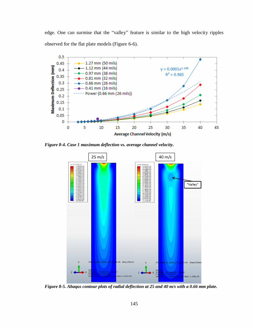
145
edge. One can surmise that the “valley” feature is similar to the high velocity ripples
observed for the flat plate models (Figure 6-6).
Figure 8-4. Case 1 maximum deflection vs. average channel velocity.
Figure 8-5. Abaqus contour plots of radial deflection at 25 and 40 m/s with a 0.66 mm plate.

146
Figure 8-6. Axial centerline deflection at 25 to 40 m/s with a 0.66 mm plate.
8.2.2 Case 2 Results
Figure 8-7 shows the maximum plate deflection as velocity increases for all plate
thicknesses. Similar to Figure 8-4 a 0.41 mm (16 mil) model at 9 m/s is included as a
prediction for a future curved plate experiment which will use a nominally 0.38 mm (15
mil) curved plate at ~9 m/s. When the velocity was increased beyond 20, 25, and 30 m/s
with the 0.66, 0.81, and 0.97 mm plate the deformation at the leading edge exhibited
irregular bending. Figure 8-8 shows contours of radial deflection at 20 and 25 m/s with a
0.66 mm (26 mils) plate. At 20 m/s the plate radially deflects into the 2.54 mm (100 mils)
channel, but at 25 m/s the plate deflects into both channels. At the midpoint of the leading
edge the plate deflects into the 2.54 mm (100 mils) channel but near the clamped edges
the plate deflects into the 2.03 mm (80 mils) channel, which is clearly shown in Figure 8-
10. Once the velocity was increased to 30 m/s the model crashed due to 19.41 mm
(0.787”) of deflection. This large deflection at 30 m/s can be seen in Figure 8-10, it
should be noted that the deformation scale factor is 1. Similar results were found with the
0.81 mm (32 mils) and 0.97 mm (38 mils) plates at 35 and 40 m/s, respectively.

147
Figure 8-7. Case 2 maximum deflection results vs. average channel velocity.
Figure 8-8. Leading edge bending into both channels at 25 m/s with a 0.66 mm plate, contour
is showing radial deflection (Case 2).

148
Figure 8-9. Excessive radial deflection into the 2.54 mm channel at 30 m/s.
Figure 8-10. Excessive radial deflection into the 2.54 mm channel at 30 m/s, deflection is 19.41
mm.

149
8.3 Comparing Flat and Curved Plates
To reveal the hydro-mechanical benefit of plate curvature, the flat plate FSI
models from Chapter 6 were compared to the curved plate FSI models. Table 8-1
compares the maximum leading edge deflection between the flat and curved plate
models. The % difference was calculated using Eq. (3.17) and it is apparent that the
curved plates are about two orders of magnitude stiffer than the flat plates. Curiously, the
% difference at 7 and 8 m/s is noticeably higher than the lower velocities. It was
discussed in Chapter 6 that the deflection profiles at 7 and 8 m/s were significantly
different that the profiles at the lower velocities. This likely explains the discrepancy
since the curved plates did not show deviations in their deflection profiles until around 25
or 40 m/s (Figure 6-6).
Table 8-1. Comparing the maximum deflection with flat and curved plates.
Deflection (mm)
Avg. Ch. Velocity (m/s)
1.02 mm (40 mils) Flat Plate
0.97 mm (38 mils) Curved Plate
% Difference
3 0.0833 0.0010 7866%
4 0.1417 0.0017 8336%
5 0.2053 0.0025 8261%
6 0.2837 0.0034 8345%
7 0.4112 0.0043 9482%
8 0.6397 0.0048 13133%
This comparison clearly shows that plate curvature has a large impact on the
magnitude of flow-induced deflections. This is promising considering the current HEU
fuel plates in the MURR core are curved and the proposed LEU fuel plates are curved.
However, these FSI models still need to be benchmarked against an experiment.
Furthermore, adding the laminate sandwich structure (detailed in Chapter 1) to the FSI
models should be explored to assure contact stress limits are not reached, which may
cause delamination of the plates.

150
CHAPTER 9 - CLOSURE
9.1 Conclusions
The five U.S. high performance research reactors, including the University of
Missouri Research Reactor (MURR), provide world-class facilities for scientists and
engineers to conduct cutting edge research, however they are currently fueled with
weapons-usable HEU fuel. In an effort to remove HEU from civilian, and in general,
global use, which is the goal of the Global Threat Reduction Initiative, these reactor are
currently working to convert to proliferation resistant LEU fuel. The proposed LEU fuel
is a foil based laminate sandwich structure, which is in contrast to the current HEU fuel’s
monolithic structure that is both thermally and mechanically robust. Questions regarding
the hydro-mechanical stability of the new LEU fuel have been raised, specifically in the
context of its structural differences as well as its required thinning. Both are required to
maintain the performance standards of the reactors.
The purpose of this research was to develop numeric tools to support the
qualification of the proposed LEU fuel within the harsh environment of a research reactor
core. Tool development included building and stabilizing fluid-structure interaction (FSI)
models to access the hydro-mechanical stability of MURR-specific geometries. Although
the MURR fuel plates are curved, initial models were built with flat plates to assess the
influence of curvature on plate deflection as well as provide an upper bound on plate
deflection. The wall clock runtime of the models was also drastically decreased to a few
days compared to previous models that took about a month to complete, while also
attaining a better understanding of why the models are unstable. A method was also
introduced for computing stable temporal step sizes as well as predicting the stability of a
model before it is started.

151
These flat plate models were then compared to experiments conducted using the
University of Missouri Hydro-Mechanical Flow Loop. Unfortunately, the models largely
failed to predict the data collected during flow experiments. The discrepancies were
tracked back to assuming perfect geometry in the models when in reality the experiment
has numerous non-uniformities in its geometry. Thus, to further increase the accuracy and
repeatability of measuring these non-uniformities a new automated positioning system
was designed and built for the flow loop’s laser displacement sensors. Finally, FSI
models were built with curved geometries to access the impact of plate curvature on plate
deflection.
9.2 Future Work
While steps have been taken to help qualify the safe-use of the proposed LEU fuel
at the MURR and other high performance research reactors, validation of the FSI models
still needs to be accomplished. To help facilitate the validation of the models, a more
prototypic representation of the experiment geometry needs to be included in the model
geometry. To accomplish this, the flow loop’s new positioning system should be utilized
to obtain a fine mapping of the experiment’s initial (no-flow) geometry using the laser
displacement sensors. A thorough understanding of this initial experiment geometry will
allow prototypic FSI models to be built. These prototypic models will undoubtedly help
facilitate matching of the predicted solutions of the models to that of the data measured in
the flow experiments.
Once the FSI models are validated against the experiment, they can be used to
model complicated geometries that would be costly to investigate experimentally. Some
of these geometries include adding the laminate sandwich structure to the plate geometry

152
and adding multiple plates to the model. Including the laminate structure will help access
the contact stresses between the layers of the plate that will likely develop during plate
deformation and including multiple plates in the model help reveal how multiple
deforming plates will interact with each other. Successful modeling with a laminate
structure will simplify adding the heating problem to the models. Quantifying thermal-
hydro-mechanical affects in the plates will be nearly impossible to accomplish in an
experiment with the high power densities that are present within these plates during
irradiation. Thus, adding the thermo-mechanical piece to the models will be essential to
successfully qualifying the proposed LEU fuel. Nonetheless, the work presented in this
thesis has laid the groundwork for validating the FSI models against the experiment,
which will help accomplish the goal of converting the five remaining U.S. high
performance research reactors from the weapons-usable HEU fuel to the proliferation
resistant LEU fuel.
Finally, more numeric studies should be completed with the FSI models in an
effort to find a better method for accessing a model’s stability. Most importantly, a spatial
mesh study should be completed to attain a better understanding of how the size of the
spatial mesh affects a model’s stability. Using the results of these numeric studies better
equations/methods can be developed for calculating stable temporal step sizes as well as
accessing the overall stability of a model based on its physical properties.

153
APPENDIX 1 – MODEL BENCHMARKING: THE ‘SNAP’ VELOCITIES
A1 1. Comparison of the model (solid lines) to the experiment (dashed lines) at ~5.47 m/s.
A1 2. Comparison of the model (solid lines) to the experiment (dashed lines) at ~5.66 m/s.

154
A1 3. Comparison of the model (solid lines) to the experiment (dashed lines) at ~5.85 m/s.
155
APPENDIX 2 – ANL MEMO: FLOW VELOCITY THROUGH MURR

156
APPENDIX 3 – MATLAB CODE FOR ANALYTIC FLOW MODEL
% This m-file calculates the pressure field for a flow field of
parallel channels % Written by Casey J. Jesse in January 2014 at the University of
Missouri - Columbia % Revisions: % % % %function [ch1,ch2] = FlowModel(V_avg,rho) %clear all k_losses = 'White'; %--------------------------------------------GEOMETRIC PARAMETERS------
-------------------------------------------- a = 0.04*0.0254; % plate thickness,
meter b = 0.08*0.0254; % channel 1 thickness,
meter c = 0.10*0.0254; % channel 2 thickness,
meter d = 4.342*0.0254; % width of plate, meter alpha = pi/8; % half of the curved
plate's arc R = d/(2*alpha); % radius of the curved
plate
L_in = 7.5*0.0254; % length of the inlet
plenum, meter L_ch = 0.6477; % length of the
plate's flow channels, meter L_out = 3*0.0254; % length of the outlet
plenum, meter
V_avg = 8.0; V_in = V_avg*(b+c)/(a+b+c); % inlet fluid velocity,
m/s rho = 997.561; % fluid density, kg/m^3 mu = 8.8871e-4; % fluid dynamic
viscosity, Pa*s
E = 6.89e10; % Young's modulus of
the plate (Al 6061 T6) v = 0.33; % Poisson's ratio of
the plate (Al 6061 T6) rho_s = 2700; % density of the plate
(Al 6061)
%----------------------------------------DERIVED PROPERTIES------------
----------------------------------- V_s = a*d*L_ch; V_f = ((a+b+c)*d*(L_in+L_ch+L_out)) - V_s;
A_in = (a+b+c)*d;

157
A_ch1 = b*d; A_ch2 = c*d;
m_s = V_s*rho_s; m_f = V_f*rho;
D_in = 2*((a+b+c)*d)/(a+b+c+d); % hydraulic diameter of
the inlet plenum, meter D_ch1 = 2*(b*d)/(b+d); % hydraulic diameter of
channel 1, meter D_ch2 = 2*(c*d)/(c+d); % hydraulic diameter of
channel 2, meter
%----------------------------------------LOSS COEFFICIENTS-------------
---------------------------------- if strcmp(k_losses, 'White') % Expansion and Contraction Coefficients from White kc_ch1 = 0.42*(1 - (b^2/((b + a/2)^2))); kc_ch2 = 0.42*(1 - (c^2/((c + a/2)^2)));
ke_ch1 = (1 - b^2/((b + a/2)^2))^2; ke_ch2 = (1 - c^2/((c + a/2)^2))^2;
D_ce_ch1 = 2*(b*d + 0.5*a*d)/(b + 0.5*a + d); D_ce_ch2 = 2*(c*d + 0.5*a*d)/(c + 0.5*a + d);
kc_ch1 = 0.42*(1 - (D_ch1^2)/(D_ce_ch1^2)); kc_ch2 = 0.42*(1 - (D_ch2^2)/(D_ce_ch2^2));
ke_ch1 = (1 - (D_ch1^2)/(D_ce_ch1^2))^2; ke_ch2 = (1 - (D_ch2^2)/(D_ce_ch2^2))^2;
elseif strcmp(k_losses,'Blevins') % Expansion and Contraction Coefficients from Blevins if b == c kc_ch1 = 0.5*(1 - (b + c)/(a + b + c)); kc_ch2 = kc_ch1;
ke_ch1 = (1 - (b + c)/(a + b + c))^2; ke_ch2 = ke_ch1; else kc_ch1 = 0.5*(1 - b/(0.5*a + b)); kc_ch2 = 0.5*(1 - c/(0.5*a + c));
ke_ch1 = (1 - b/(0.5*a + b))^2; ke_ch2 = (1 - c/(0.5*a + c))^2; end else % Expansion and Contraction Coefficients from John's Numeric Model kc_ch1 = 0.205; kc_ch2 = 0.1275;
ke_ch1 = 0.1501;

158
ke_ch2 = -0.138; end
%------------------------------------------PROPERTIES OF THE FLOW------
-------------------------------------------- Re_in = V_in*rho*D_in/mu; % Reynold's number
through the inlet plenum Re_avg = V_avg*rho*D_ch1/mu; % Reynold's number
through channels Le_in = 4.4*Re_in^(1/6)*D_in; % entrance length for
fully developed flow (approximate), meter Le_ch = 4.4*Re_avg^(1/6)*D_ch1; % entrance length for
fully developed flow (approximate), meter
V_miller = ((30*E*a^3*0.09*0.0254)/(rho*d^4*(1-v^2)))^0.5;
%------------------------------------------SOLVING FOR CH VELOCITES----
-------------------------------------------- i = 1; V_ch1 = V_avg; % intial guess for
Newton Raphson V_ch2 = V_in*A_in/A_ch2 - V_ch1*A_ch1/A_ch2; error = 1; for i = 1:10 V_prev = V_ch1;
log_ch1 = log(6.9*mu/(rho*V_ch1*D_ch1)); log_ch2 = log(6.9*mu/(rho*D_ch2*(V_in*A_in/A_ch2 -
V_ch1*A_ch1/A_ch2)));
f1 = (rho*V_ch1^2/2)*(kc_ch1 + (-
log(10)/(1.8*log_ch1))^2*L_ch/D_ch1 + ke_ch1); f2 = rho/2*V_ch2^2*(kc_ch2 + (-log(10)/(1.8*log_ch2))^2*L_ch/D_ch2
+ ke_ch2);
f = f1 - f2;
df1 = rho*V_ch1*(kc_ch1 + ke_ch1); df2 = rho/2*L_ch/D_ch1*(3.27278*V_ch1/(log_ch1^3) +
3.27278*V_ch1/(log_ch1^2)); df3 = rho/2*(2*A_ch1*V_ch2*(kc_ch2 + ke_ch2 +
1.63639*L_ch/(D_ch2*log_ch2^2))/A_ch2); df4 = rho/2*(3.27278*A_ch1*L_ch*V_ch2/(A_ch2*D_ch2*log_ch2^3)); df = df1 + df2 + df3 + df4;
% Computing the new velocity in channel 1 and channel 2 V_ch1 = V_prev - f/df; V_ch2 = V_in*A_in/A_ch2 - V_ch1*A_ch1/A_ch2;
% Computing the error in the newly calculated velocity in channel 1 error = abs((V_ch1 - V_prev)/V_prev); if error < 1e-10 break end end

159
fprintf('The velocity in channel 1 is %f m/s \n', V_ch1); fprintf('The velocity in channel 2 is %f m/s \n', V_ch2);
m_dot_1 = V_ch1*b*d*rho; m_dot_2 = V_ch2*c*d*rho;
%---------------------------------------CONTRIBUTION FROM BERNOULLI----
------------------------------------------ % There will be a contribution from Bernouilli at the inlet and outlet
of the channels from the area changes dP_B1 = 0.5*rho*(V_ch1^2 - V_in^2); dP_B2 = 0.5*rho*(V_ch2^2 - V_in^2); %---------------------------------------CREATING PRESSURE PROFILE PLOT-
--------------------------------------------- % Pressure drop through the outlet plenum f_out = (-log(10)/(1.8*log(6.9/Re_in)))^2; dP_out = f_out*L_out*V_in^2*rho/(2*D_in); fprintf('The pressure drop through the outlet plenum is %f
Pa\n',dP_out);
% Pressure drop from the sudden expansion from channel 1 dP_e1 = 0.5*ke_ch1*rho*V_ch1^2; fprintf('The pressure recovery from the expansion from the channel 1 is
%f Pa\n',dP_e1);
% Pressure drop from the sudden expansion from channel 2 dP_e2 = 0.5*ke_ch2*rho*V_ch2^2; fprintf('The pressure recovery from the expansion from channel 2 is %f
Pa\n',dP_e2);
% Pressure drop from the friction in channel 1 Re_ch1 = rho*V_ch1*D_ch1/mu; f_ch1 = (-log(10)/(1.8*log(6.9/Re_ch1)))^2; dP_ch1 = f_ch1*L_ch*V_ch1^2*rho/(2*D_ch1); fprintf('The pressure drop through channel 1 is %f Pa\n',dP_ch1);
% Pressure drop from the friction in channel 2 Re_ch2 = rho*V_ch2*D_ch2/mu; f_ch2 = (-log(10)/(1.8*log(6.9/Re_ch2)))^2; dP_ch2 = f_ch2*L_ch*V_ch2^2*rho/(2*D_ch2); fprintf('The pressure drop through channel 2 is %f Pa\n',dP_ch2);
% Pressure drop from the contraction into channel 1 dP_c1 = 0.5*kc_ch1*rho*V_ch1^2; fprintf('The pressure drop from the contraction from the channel 1 is
%f Pa\n',dP_c1);
% Pressure drop from the contraction into channel 2 dP_c2 = 0.5*kc_ch2*rho*V_ch2^2; fprintf('The pressure drop from the contraction from the channel 2 is
%f Pa\n',dP_c2);
% Pressure drop from the friction in the inlet plenum f_in = (-log(10)/(1.8*log(6.9/Re_in)))^2; dP_in = f_in*L_in*V_in^2*rho/(2*D_in);

160
fprintf('The pressure drop through the inlet plenum is %f Pa\n',dP_in);
% Total pressure drop through the model dP_total_ch1 = dP_out + dP_e1 + dP_ch1 + dP_c1 + dP_in; dP_total_ch2 = dP_out + dP_e2 + dP_ch2 + dP_c2 + dP_in; deltaP = dP_total_ch1; fprintf('The pressure drop throught the entire 1D model is %f
Pa\n',dP_total_ch1);
P_out = 0; P_chOut = dP_out;
P_chExp1 = P_chOut + dP_e1 - dP_B1; P_chIn1 = P_chExp1 + dP_ch1; P_chCon1 = P_chIn1 + dP_c1 + dP_B1;
P_chExp2 = P_chOut + dP_e2 - dP_B2; P_chIn2 = P_chExp2 + dP_ch2; P_chCon2 = P_chIn2 + dP_c2 + dP_B2;
P_in1 = P_chCon1 + dP_in; P_in2 = P_chCon2 + dP_in;
% Total pressure difference at the leading of the plate dP = P_chIn1 - P_chIn2; fprintf('The differential pressure at the plates leading edge is %f
Pa\n',dP);
ch1 = P_in1; ch2 = P_in2;
PLOT = 0; if PLOT == 1 x = [-L_out, 0, 0, L_ch, L_ch, L_in+L_ch]; ch1 = [0, P_chOut, P_chExp1, P_chIn1, P_chCon1, P_in1]; ch2 = [0, P_chOut, P_chExp2, P_chIn2, P_chCon2, P_in2]; figure(1) plot(x,ch1, 'r-', 'LineWidth', 2);hold on;grid on plot(x,ch2, 'b-', 'LineWidth', 2);hold off xlabel('Location (m)') ylabel('Pressure (Pa)') legend('Channel 1', 'Channel 2', 'Location', 'NorthWest') end

161
APPENDIX 4 – MATLAB CODE FOR ANALYTIC PLATE MODEL
% This m-file calculates deflection of a flat plate using beam theory % Written by Casey J. Jesse in August 2014 at the University of
Missouri - Columbia % Revisions: % clear all;clc %close all a = 0.04*0.0254; % plate
thickness, m b = 4.342*0.0254; % plate
width, m L = 0.6477; % plate length,
m
E = 6.89e10; % Elastic
Modulus, Pa v = 0.33; % Poisson's
Ratio, (-) I = a^3/12; % Area
Moment of Inertia, m^3
P = @(y) (12589*y - 396.65); % pressure loading, Pa
x = linspace(0,b,1000); y = linspace(0,L,101); del = zeros(1,length(x)); del_max = zeros(length(y),1); for k = 1:1 for j = 1:length(y) p = P(y(j)); %p = 5000; del_max(j,1,k) = p*b^4/(384*E*I)*(1-v^2); for i = 1:length(del) del(j,i,k) = p*x(i)^2/(24*E*I)*(2*b*x(i) - b^2 -
x(i)^2)*(1-v^2); end end end
figure(1) plot(x,del(100,:));grid on xlabel('Plate Width (m)');ylabel('Deflection (mil)') fprintf('The maximum deflection along the plate is %f mm (%f
mils)\n',max(del_max)*1000,max(del_max)/0.0254*1000)
figure(2) [X Y] = meshgrid(x,y); surf(X,Y,del(:,:,1)*-1000);shading interp;colorbar('Location','North') %set(gca, 'CLim', [-3.6e-1, 2e-2]); axis equal axis([0 b 0 L]) xlabel('Width (m)');ylabel('Length (m)'); view(90,90);

162
REFERENCES
[1] International Atomic Energy Agency, "Pioneering Nuclear Science: The Discovery
of Nuclear Fission," 24 February 2015. [Online]. Available:
https://www.iaea.org/newscenter/news/pioneering-nuclear-science-discovery-
nuclear-fission. [Accessed 28 February 2015].
[2] Argonne National Laboratory, "FRONTIERS Research Highlights 1946-1996,"
Office of Public Affairs, Argonne National Laboratory, Chicago, 1996.
[3] F. G. Gosling, The Manhattan Project Making the Atomic Bomb, Department of
Energy, 2010.
[4] J. Varnum, "Nuclear Enginering International," 23 January 2014. [Online].
Available: http://www.neimagazine.com/features/feature60-years-of-atoms-for-
peace-4164653/. [Accessed 17 October 2014].
[5] International Atomic Energy Agency (IAEA), "Mangement of high enriched
uranium for peacefule purposes: Status and trends," IAEA, Vienna, 2005.
[6] D. Albright and K. Kramer, "ISIS Civel HEU Watch," August 2006. [Online].
Available: http://isis-online.org/uploads/isis-
reports/documents/civil_heu_watch2005.pdf. [Accessed 17 October 2014].
[7] Z. Mian and A. Glaser, "A Frightening Nuclear Legacy," Bulletin of the Atomic
Sciences, 64 (4), pp. 42-47, September/October 2008.
[8] A. Loukianova and C. Hansell, "Leveraging U.S. Policy for a Global Commitment
to HEU Elimination," The Nonproliferatoin Review, pp. 159-183, 2008.
[9] National Nuclear Security Administration (NNSA), "GTRI's Convert Program:
Minimizing the Use of Highly Enriched Uranium," 29 May 2014. [Online].
Available: https://nnsa.energy.gov/mediaroom/factsheets/gtri-convert. [Accessed 17
October 2014].
[10] International Atomic Energy Agency, "The Role of Research Reactors in
Introducing Nuclear Power," [Online]. Available:
http://www.iaea.org/About/Policy/GC/GC56/GC56InfDocuments/English/gc56inf-
3-att5_en.pdf. [Accessed 17 October 2014].
[11] International Atomic Energy Agency, "Research Reactors: Purposes and Future,"
IAEA, Vienna, 2010.
[12] D. Wachs, "Coneptual Process Description for the Manufacture of Low-Enriched
Uranium-Molybdenum Fuel," Idaho National Laboratory, Idaho Falls, 2008.
[13] J. C. McKibben, "Feasibility Analysis for HEU to LEU Fuel Conversion of the
University of Missouri Research Reactor (TDR-0125)," University of Missouri
Research Reactor, Columbia, MO, 2011.
[14] J. Stillman, "Technical Basis in Support of the Conversion of the University of
Missouri Research Reactor (MURR) Core from Highly-Enriched to Low-Enriched
Uranium - Core Neutron Physics," Argonne National Laboratory, Chicago, 2012.
[15] H. M. Kristensen and R. S. Norris, "Worldwide Depolyments of Nuclear Weapons,
2014," Bulletin of the Atomic Scientists, 1 September 2014.

163
[16] Nuclear Threat Initiative, "Understanding Nuclear Threats," [Online]. Available:
http://www.nti.org/threats/nuclear/. [Accessed 22 October 2014].
[17] CD-Adapco, Star-CCM+ (Version 7.04.011 and 9.02.007-R8) [Software], 2014.
[18] Simulia, Abaqus CAE (Version 6.12-2 and 6.13-1) [Software], Simulia, 2013,2014.
[19] D. R. Miller, "Critical Flow Velocities for Collapse of Reactor Parallel-Plate Fuel
Assemblies," Transactions of the ASME Journal of Engineering for Power, vol.
April 1960, pp. 83-91, 1960.
[20] E. B. Johansson, "Hydraulic Instability of Reactor Parallel-Plate Fuel Assemblies,"
United States Atomic Energy Commission, Schenectady, New York, 1959.
[21] G. S. Rosenberg and C. K. Youngdahl, "A Simplified Dynamic Model for the
Vibration Frequencies and Critical Coolant Flow Velocities for Reactor Parallel
Plate Fuel Assemblies," Nuclear Science and Engineering, vol. 13, no. 2, 1962.
[22] J. J. Kane, "The Effect of Inlet Spacing Deviations on the Flow-Induced Deflections
of Flat Plates," Nuclear Science and Engineering, vol. 15, 1963.
[23] R. J. Scavuzzo, "Hydraulic Instability of Flat Parallel-Plate Assemblies," Nuclear
Science and Engineering, no. 21, pp. 463-472, 1965.
[24] M. W. Wambsganss, "Second-Order Effects as Related to Critical Coolant Flow
Velocities and Reactor Parallel Plate Fuel Assemblies," Nuclear Science and
Engineering, no. 5, pp. 268-272, 1967.
[25] P. Jensen and W. Marcum, "Predicting Critical Flow Velocity Leading to Laminate
Plate Collapse - Flat Plates," Nuclear Engineering and Design, no. 267, pp. 71-87,
2014.
[26] W. R. Marcum, "Predicting Critical Flow Velocity Leading to Laminate Plate
Collapse - Cylindrical Plates," Nuclear Engineering and Design, no. 278, pp. 50-63,
2014.
[27] W. L. Zabriskie, "An Experimental Evaluation of the Critical Flow Velocity
Formulas for Parallel Plate Assemblies," General Electric Co., Schenectady, N.Y.,
1958.
[28] W. L. Zabriskie, "An Experimental Evaluation of the Effect of Length-to-Width
Ratio on the Critical Flow Velocity of Single Plate Assemblies," General Electric
Co., Schenectady, N.Y., 1959.
[29] R. D. Groninger and J. J. Kane, "Flow Induced Deflections of Parallel Flat Plates,"
Nuclear Science and Engineering, no. 16, pp. 218-226, 1963.
[30] G. E. Smissaert, "Hydroelastic Instabilities in MTR-Type Fuel Elements," Nuclear
Engineering and Design, no. 7, pp. 535-546, 1968.
[31] M. Ho, G. Hong and A. F. Mack, "Experimental Investigation of Flow-Induced
Vibration in a Parallel Plate Reactor Fuel Assembly," in Australasian Fluid
Mechanics Conference, Sydney, Australia, 2004.
[32] L. Lifang, L. Daogang, L. Yang, Z. Pan and N. Fenglei, "Large-Amplitude and
Narrow-Band Vibration Phenomenum of a Foursquare Fix-Supported Flexible Plate
in Rigid Narrow Channel," Nuclear Engineering and Design, vol. 241, pp. 2874-
2880, 2011.

164
[33] Y. Li, L. Daogang, Z. Pan and L. Lifang, "Experimental Investigation on Fluid–
Structure Interaction Phenomenon Caused by the Flow through Double-Plate
Stucture in a Narrow Channel," Nuclear Engineering and Design, vol. 248, pp. 66-
71, 2012.
[34] C. A. Felippa, K. C. Park and C. Farhat, "Partitioned Analysis of Coupled
Mechanical Systems," Departmetn of Aerospace Engineering Studies and Center of
Aerospace Structures University of Colorado Boulder, Boulder, CO, 1999.
[35] S. Piperno and C. Farhat, "Partitioned Procedures for the Transient Solution of
Coupled Aeroelastic Problems - Part II: Energy Transfer and Three-Dimensional
Applications," Computer Methods in Applied Mechanics and Engineering, vol. 190,
pp. 3147-3170, 2001.
[36] P. Causin, J. F. Gerbeau and F. Nobile, "Added-mass effect in the design of
partitioned algorithms for fluid-structure problems," Computer Methods in Applied
Mechanics and Engineering, no. 194, pp. 4506-4527, 2005.
[37] C. Forster, W. A. Wall and E. Ramm, "Artificial added mass instabilities in
sequential staggered coupling of nonlinear structures and incompressible viscous
flows," Computer Methods in Applied Mechanics and Engineering, no. 196, pp.
1278-1293, 2007.
[38] F. Nobile, Numerical Approximation of Fluid-Structure Interaction Problems with
Applications to Haemodynamics, Ph.D. thesis, EPFL, Switzerland, 2001.
[39] R. Courant, K. Friedrichs and H. Lewy, "On the Partial Difference Equations of
Mathematical Physics (Translation of Uber die partiellen Differenzengleichungen
der mathematishen Physik, 1928)," AEC Computing Facility, New York, New York,
1956.
[40] F. M. White, Fluid Mechanics, New York: McGraw-Hill, 2008.
[41] CD-Adapco, "Star-CCM+ Documentation," CD-Adapco, New York, 2014.
[42] S. V. Patankar, Numerical Heat Transfer and Fluid Flow, Taylor and Francis, 1980.
[43] T. V. Karman, "Mechanical Similitude and Turbulene," National Advisory
Committee for Aeronautics, Washington, 1931.
[44] ASM Aerospace Specifications Inc., "Aluminum 6061-T6,; 6061-T651," [Online].
Available:
http://asm.matweb.com/search/SpecificMaterial.asp?bassnum=MA6061t6.
[Accessed 26 February 2015].
[45] W. C. Young and R. G. Budynas, Roark's Formulas for Stress and Strain, New York:
McGraw-Hill, 2002.
[46] Simulia, "Abaqus CAE Documentation," Simulia, Providence, RI, 2014.
[47] J. C. Kennedy and G. L. Solbrekken, "Coupled Fluid Structure Interaction (FSI)
Modeling of Parallel Plate Assemblies," in ASME International Mechanical
Engineering Congress & Exposition, Denver, Colorado, 2011.
[48] J. C. Kennedy, C. J. Jesse, R. W. Slater and G. L. Solbrekken, "Fluid-Structure
Interaction Modeling and Experimetal Benchmarking Status," University of
Missouri TherMec Lab Research Group, Columbia, MO, 2012.

165
[49] A. Mueller, "Strategies for Improving Stability of Explicit Coupling," CD-Adapco,
2011.
[50] J. C. Tannehill, D. A. Anderson and R. H. Pletcher, Computational Fluid Mechanics
and Heat Transfer, Washington: Taylor & Francis, 1997.
[51] J. C. Kennedy, R. W. Slater, J. A. Moreland, K. D. East and G. L. Solbrekken,
"Missouri Hydro-Mechanical Flow Loop: Equipment Specifications and Usage
Requirements (TDR-MU-EXP-201203-001A)," University of Missouri TherMec
Lab, Columbia, MO, 2012.
[52] J. C. Kennedy, C. J. Jesse and G. L. Solbrekken, "Experimental Investigation of
Deflection of Flat Aluminum Plates Under Variable Velocity Parallel Flow,"
Columbia, MO, 2014.
[53] Helix Linear Technologies, "The Engineer's Guide: Lead Screws vs. Ball Screws,"
[Online]. Available: http://blog.helixlinear.com/bid/224687/Lead-Screws-vs-Ball-
Screws-It-s-All-about-the-Application. [Accessed 26 February 2015].
[54] UL Prospector, "Polylactic Acid (PLA) Typical Properties," [Online]. Available:
http://plastics.ulprospector.com/generics/34/c/t/polylactic-acid-pla-properties-
processing. [Accessed 26 February 2015].
[55] FundingUniverse, "Stratasys, Inc. History," FundingUniverse, [Online]. Available:
http://www.fundinguniverse.com/company-histories/stratasys-inc-history/.
[Accessed 25 February 2015].
[56] C. Daniels, Slic3r [open source software], 2014.
[57] Hot-World GmbH & Co. KG, Repetier-Host [open source software], Germany.
[58] RepRap Project, "Prusa Mendel (iteration 2)," 2015. [Online]. Available:
http://reprap.org/wiki/Prusa_Mendel_%28iteration_2%29. [Accessed 25 February
2015].
[59] ReRap Project, "Kossel," 2015. [Online]. Available: http://reprap.org/wiki/Kossel.
[Accessed 25 February 2015].
[60] L. Foyto, K. Kutikkad, J. C. McKibben, N. Peters, G. Solbrekken, E. Feldman, J.
Stevens, J. Stillman and C. Tzanos, "Preliminary Safety Analysis Report
Methodologies and Scenarios for LEU Fuel Conversion of the University of
Missouri Research Reactor (MURR)," University of Missouri and Argonne National
Laboratory, Columbia, MO, 2011.
[61] CNC Cookbook, "CNC Machine Overview and Computer Numerical Control
History," CNC Cookbook, 2010-2014. [Online]. Available:
http://www.cnccookbook.com/CCCNCMachine.htm. [Accessed 25 February 2015].