analysis of the relative contributions -(hydrographs) of the sub-catchments during the flood
TRANSCRIPT

Analysis of the relative contributions -
(hydrographs) of the sub-catchments during the flood

Contents
Interpolated Rainfall :« simple to complexe » methods
Hydrographs calculation SCS Method
Calibration of MIKE SHE for the VAR catchments Parameters, values, graphs
Contribution analysis during the floodCalibration???Conclusions

Rainfall Interpolation Methods :« simple to complexe »
Homogeneous Rainfall on the sub-catchment
Thiessen Method
Kriging Method
Hypothesis : Spatial distribution of the rainfall are the same on the all catchment=> mean of the six rain gauges station
o Homogeneous Rainfall on the sub-catchment

Rainfall Interpolation Methods :« simple to complexe »
o Thiessen Method
• Thiessen Polygon (ARCGIS)
• Assigning to each station an influence area (%) that represents weighting factor.
• To calculate the interpolated rain :
∑ rainfall for each station x weighting factor ---------------------------------------------------- Total area conerning
Tinée Upper Var Vésubie Down Var Esteron
Carros 0 0 0 64 8
Levens 6 2 22 36 7
Roquesteron 0 7 0 0 46
Puget Théniers 0 38 0 0 39
Guillaumes 48 53 0 0 0
St Martin de Vésubie 47 0 78 0 0
• Estimating rainfall weighted taking into account each station.

Rainfall Interpolation Methods :« simple to complex »
o Kriging Method
Interpolation by kriging for each sub-catchment and for each hour
Hydrographs calculation
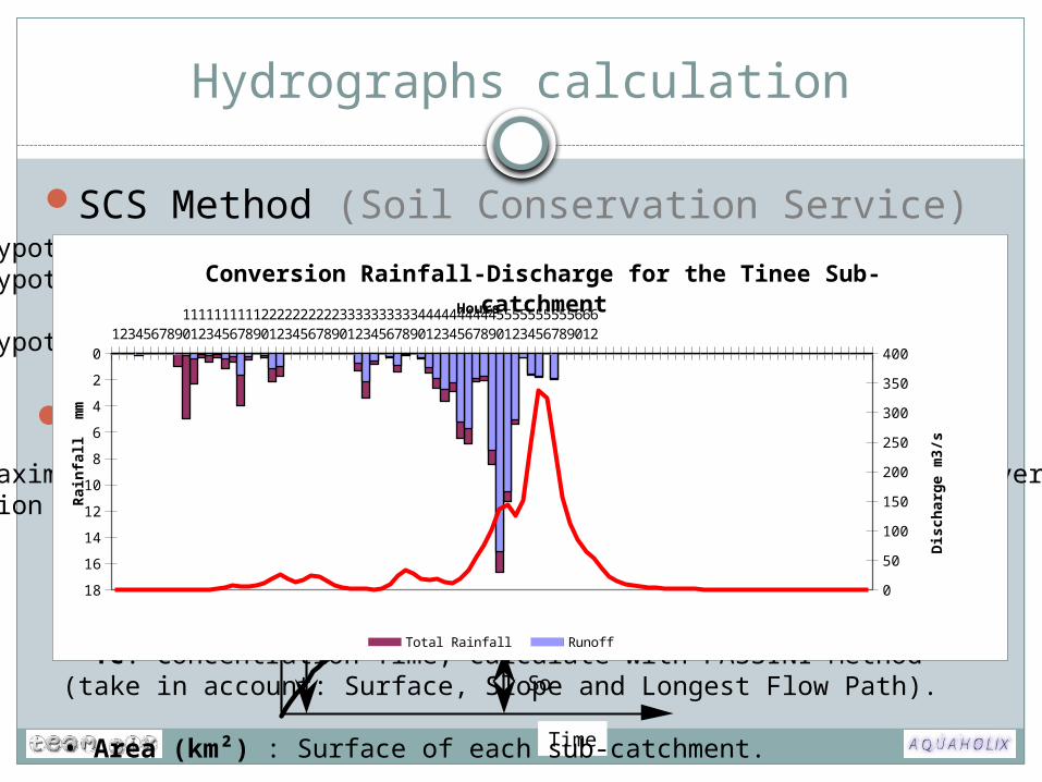
SCS Method (Soil Conservation Service) Hypothesis 1: Infiltration capacity tends to zero as time increases.Hypothesis 2: Runoff appear after it dropped some rainfall.
Hypothesis 3: R (t) = [ si Pu (t) > 0 ]
Temps
Lames d'eau cumulées
R(t)
Pu(t)P(t)
So
S
Temps infini
0
t
J(t) dt
Cumulated Water
Finish Time
Time
)t(PS
)t(P
u
2u
SCS Parameters:• S: Maximum infiltration capacity, depend on Soil characteristics, cover, condition of initial wetting.
Tinée Upper Var Vésubie Down Var Esteron SCS Value 85 85 85 30 80• Tm: Time of the peak discharge, base on Concentration Time ( Tm
= 3/8 Tc). • Tc: Concentration Time, calculate with PASSINI Method (take in account: Surface, Slope and Longest Flow Path).
• Area (km²) : Surface of each sub-catchment.
1234567891011121314151617181920212223242526272829303132333435363738394041424344454647484950515253545556575859606162
0
2
4
6
8
10
12
14
16
18 0
50
100
150
200
250
300
350
400
Conversion Rainfall-Discharge for the Tinee Sub-catchment
Total Rainfall Runoff
Hours
Rai
nfa
ll
mm
Dis
char
ge
m3/
s

Hydrographs calculation
SCS Result:
Catég
orie
1
Catég
orie
2
Catég
orie
3
Catég
orie
40
2
4
6
Série 1Série 2Série 3
• Almost no big differences appear between the rainfall distribution results from the Thiessen and the homogeneous method
• The discharge value are globally in accord with calculate value in the Napoleon Bridge
• Except for Surfer method. Doesn’t take in account the different landuse, the slope or the topography. With more than we could obtain better result including topography in Surfer.
• Homogeneous discharge is more important than the Thiessen value. Due to Thiessen method take in account spatial reference of the station.
11
/04
/19
94
/ 1
1 0
0
13
00
15
00
17
00
19
00
21
00
23
00
11
/05
/19
94
/ 0
1 0
0
03
00
05
00
07
00
09
00
11
00
13
00
15
00
17
00
19
00
21
00
23
00
11
/06
/19
94
/ 2
4 0
0
04
00
06
00
08
00
10
00
12
00
14
00
16
00
18
00
20
00
22
00
24
00
0
500
1000
1500
2000
2500
3000
3500
4000
4500
5000 Hydrographs for the Var’s Catchment
Time (hours)
Discharge (m3/s)
Kriging
Napoléon B.
Thiessen
Homogen-eous.

Tinee hydrograph
Hydrographs calculation
SCS Result:
Discharge (m3/s)
Contributions of the sub-catchments during the flood (%)
Tm (hours)
Tinee 1177,8 28 8
Vésubie 869,1 20 5
UpperVar 1204 28 12
DownVAr 336 8 4
Estéron 689 16 8

Calibration of MIKE SHE
First calibration-using only MIKE SHE Using: 300 m grid sizeExperiences : very little peak of runoff
the width of the imagined river bed is 1500 m
Reasons: big grid size too big width ofriver bed, big hydraulic radius and little water
depthlittle velocity and discharge
Conclusion: we have to use river network for modelling
coupling with MIKE11
overland flow in y-direction [m^3/s]
00:001994-11-05
04:00 08:00 12:00 16:00 20:00 00:0011-06
-45
-40
-35
-30
-25
-20
-15
-10
-5
0

Calibration of MIKE SHE and coupling with MIKE 11
Parameters:IWD - Initial Water depth 0,00-0,005DS – Detention storage 0,00-0,05 Manning number (overland)10,0-40,0Net Rainfall Fraction 0,90-0,95

Calibration of MIKE SHE and coupling with MIKE 11
Parameters of the best calibration: M=24 m1/3/sNRF=0.93IWD = 0.000 mDS= 0.00 mm
Results of calibration: Peak of discharge Qc= 3701 m3/s Qm= 3680m3/s
Wrong time of the peak 2.5 hours differences sensitivity analysis not sensitive M,IWD,NRF little
sensitive DS Conclusions: We can’t calibrate more accurately under these conditions (300
grid size) and It’s not necessery because there are not observed data!

Contributions analysis
The runoff’s peak and timing depends on the following parameters:
Shape of the catchmentLanduse surface roughnessTopographyRainfall, Area
Var sub-catchments:same Landuse more than 90% forest and natural area except Down Var sub-catchment similar topography
Differences: rainfall, area, shape of the sub-catchments

Contributions analysis
Similar runoff characteristic on every sub-catchmentRelative contributions of runoff: Q%=∑Q/Qi A%=∑A/Ai
Esteron:20% c= Q%/A%=128%
Vesubie:8% c=57%Tineé: 32% c=120%Upper Var: 36% c=93% Down Var: 4% c=74%

Calibration ???
Similar runoff characteristic on every sub-catchmentRelative contributions of runoff: Esteron:21%
Vesubie:5%Tineé: 36%Upper Var: 36,5%
Down Var: 1,5%

Calibration ???

Conclusions
The relative contribution of sub-catchments only depends on the distribution of rainfall.
The Tinee, Upper Var, Esteron gave more than 90% of the whole runoff.
CONCLUSIONS OF MIKE PART:If we calculate the relative contributions of the sub-catchments (during the flood), we don’t need to use calibrated modell, because the relative contribution is not sensitive for the calibrated parameters.

TEAM SIX. . .
Thank for your attention