U.S. Department of the Interior U.S. Geological Survey

Analysis of the Variability in Ground-Motion Synthesis and Inversion

By Paul Spudich, Antonella Cirella, Laura Scognamiglio, and Elisa Tinti

Open-File Report 2017–1151

Final Report of Task 4 of Nuclear Regulatory Commission Job Code V6240 “NGA-East Ground Motion Support” September 25, 2017

U.S. Department of the Interior RYAN K. ZINKE, Secretary

U.S. Geological Survey William H. Werkheiser, Acting Director

U.S. Geological Survey, Reston, Virginia: 2017

For more information on the USGS—the Federal source for science about the Earth, its natural and living resources, natural hazards, and the environment—visit https://www.usgs.gov/ or call 1–888–ASK–USGS (1–888–275–8747).

For an overview of USGS information products, including maps, imagery, and publications, visit https://store.usgs.gov/.

Any use of trade, firm, or product names is for descriptive purposes only and does not imply endorsement by the U.S. Government.

Although this information product, for the most part, is in the public domain, it also may contain copyrighted materials as noted in the text. Permission to reproduce copyrighted items must be secured from the copyright owner.

Suggested citation: Spudich, P., Cirella, A., Scognamiglio, L., and Tinti, E., 2017, Analysis of the variability in ground-motion synthesis and inversion: U.S. Geological Survey Open-File Report 2017–1151, 39 p., https://doi.org/10.3133/ofr20171151.

ISSN 2331-1258 (online)

Acknowledgments

We thank reviewers Sarah Minson of the U.S. Geological Survey (USGS) and Rasool Anooshehpoor of the U.S. Nuclear Regulatory Commission (USNRC) for their helpful technical reviews. We thank Regan Austin, Carolyn Donlin, and Michael Diggles of the USGS Menlo Park Publishing Service Center for their advice in guiding us through the publication procedure and their work of formatting the text for publication. This work was funded in part by the National Earthquake Hazards Program of the USGS, the Istituto Nazionale di Geofisica e Vulcanologia, Italy, and Job Code V6240 of the USNRC. This paper was prepared as an account of work sponsored by an agency of the U.S. Government. Neither the U.S. Government nor any agency thereof, nor any of their employees, makes any warranty, expressed or implied, or assumes any legal liability or responsibility for any third party’s use, or the results of such use, of any information, apparatus, product, or process disclosed in this report, or represents that its use by such third party would not infringe privately owned rights. The views expressed in this paper are not necessarily those of the U.S. Nuclear Regulatory Commission.

iii

Contents Introduction .................................................................................................................................................... 1 A Discretized Frequency-Domain Derivation of Yagi and Fukahata’s (2011) Theory, with Additions

and Comments ........................................................................................................................................ 2 The Continuous-Integral Case ....................................................................................................................... 7 Estimating the Covariance Matrix of Green’s Function Errors ..................................................................... 10

The 2009 L’Aquila, central Italy, Earthquake and Aftershock Sequence .................................................. 10 Recovering Tractions from Ground Velocity ............................................................................................. 16 Covariance as a Function of Separation on the Fault ............................................................................... 20 A Covariance Model ................................................................................................................................. 25 Epistemic Error of Finite-Source Synthetic Seismograms ........................................................................ 27

Use of Epistemic Ground-motion Variance 2τ in a Simulated Annealing Inversion .................................... 31 A Cost Function Related to chi-squared ................................................................................................... 31 Cost Function Based on Correlation of Rupture Parameters .................................................................... 33 Combined Cost Function .......................................................................................................................... 34

Discussion ................................................................................................................................................... 34 Summary ..................................................................................................................................................... 35 References Cited ......................................................................................................................................... 36 Appendix 1. The Multidimensional Delta Method (MDM) ............................................................................. 38

Application to the Ground-Motion Problem ............................................................................................... 38

Figures 1. Plot of three covariance functions for heterogeneous velocity-structure models .............................. 9 2. Map of the L’Aquila, Italy, region, modified from Cirella and others (2009) ..................................... 11 3. Map of the L’Aquila, Italy, area showing focal mechanisms of 41 selected aftershocks. ................ 12 4. Plots of observed aftershock ground velocity and synthetic velocity for aftershocks 02–52, plotted at same

scale as observations, for receiver-function velocity structure at station AQU ................................ 13 5. Plots of observed aftershock ground velocity and synthetic velocity for aftershocks 53–87, plotted at same

scale as observations, for receiver-function velocity structure at station AQU 14 6. Plots of observed aftershock ground velocity and synthetic velocity for aftershocks 01–20, plotted at same

scale as observations, for CIA velocity structure at station FIAM ................................................... 15 7. Plots of observed aftershock ground velocity and synthetic velocity for aftershocks 21–33, plotted at same

scale as observations, for CIA velocity structure at station FIAM ................................................... 16 8. Argand plot of complex differences between real and synthetic ground velocities as a function of frequency

at station AQU, using CIA model .................................................................................................... 19 9. Argand plot of complex differences between real and synthetic ground velocities as a function of frequency

at station AQU, using receiver-function model ................................................................................ 19 10. Plot of real part (blue plus signs) of the covariance data formed from rigidity- and moment-scaled data for

all three components of motion at station AQU, using receiver-function velocity model for the 0.2667–0.3000-Hz frequency band ............................................................................................................. 21

11. Plot of imaginary part (blue plus signs) of covariance data formed from rigidity- and moment-scaled data for all three components of motion at station AQU, using receiver-function velocity model for the 0.2667–0.3000-Hz frequency band ............................................................................................................. 22

iv

12. Plot of median covariance as a function of separation distance in 10 frequency bands for station AQU, using receiver-function velocity model and lumping data from all components of motion together . 23

13. Plot of median covariance at station AQU as a function of separation distance for 10 frequency bands, lumping all components of motion together and normalizing to unit amplitude at smallest separation ....................................................................................................................................................... 24

14. Plot of median covariance at station FIAM as a function of separation distance for 10 frequency bands, lumping all components of motion together and normalizing to unit amplitude at the smallest separation ....................................................................................................................................................... 25

15. Plot of covariance at zero separation for various combinations of component and frequency bands for three components of motion at stations AQU and FIAM .......................................................................... 27

16. Best fitting L’Aquila mainshock-rupture model ................................................................................ 28 17. Plot of τ as a function of frequency for station AQU, using receiver-function velocity model ........ 29 18. Plot of τ as a function of frequency for station AQU, using receiver-function velocity structure .... 30 19. Plot of τ as a function of frequency for station FIAM, using CIA velocity structure ........................ 31 20. Plot of X ( )m mq values for 0 1mq≤ ≤ and for three values of γ ................................................. 33

Tables 1. Notation variations between this report and Yagi and Fukahata (2011) ........................................... 3

Analysis of the Variability in Ground-Motion Synthesis and Inversion

By Paul Spudich1, Antonella Cirella,2 Laura Scognamiglio,2 and Elisa Tinti2

Introduction In almost all past inversions of large-earthquake ground motions for rupture behavior, the goal

of the inversion is to find the “best fitting” rupture model that predicts ground motions which optimize some function of the difference between predicted and observed ground motions. This type of inversion was pioneered in the linear-inverse sense by Olson and Apsel (1982), who minimized the square of the difference between observed and simulated motions (“least squares”) while simultaneously minimizing the rupture-model norm (by setting the null-space component of the rupture model to zero), and has been extended in many ways, one of which is the use of nonlinear inversion schemes such as simulated annealing algorithms that optimize some other misfit function. For example, the simulated annealing algorithm of Piatanesi and others (2007) finds the rupture model that minimizes a “cost” function which combines a least-squares and a waveform-correlation measure of misfit.

All such inversions that look for a unique “best” model have at least three problems. (1) They have removed the null-space component of the rupture model—that is, an infinite family of rupture models that all fit the data equally well have been narrowed down to a single model. Some property of interest in the rupture model might have been discarded in this winnowing process. (2) Smoothing constraints are commonly used to yield a unique “best” model, in which case spatially rough rupture models will have been discarded, even if they provide a good fit to the data. (3) No estimate of confidence in the resulting rupture models can be given because the effects of unknown errors in the Green’s functions (“theory errors”) have not been assessed. In inversion for rupture behavior, these theory errors are generally larger than the data errors caused by ground noise and instrumental limitations, and so overfitting of the data is probably ubiquitous for such inversions.

Recently, attention has turned to the inclusion of theory errors in the inversion process. Yagi and Fukahata (2011) made an important contribution by presenting a method to estimate the uncertainties in predicted large-earthquake ground motions due to uncertainties in the Green’s functions. Here we derive their result and compare it with the results of other recent studies that look at theory errors in a Bayesian inversion context particularly those by Bodin and others (2012), Duputel and others (2012), Dettmer and others (2014), and Minson and others (2014).

Notably, in all these studies, the estimates of theory error were obtained from theoretical considerations alone; none of the investigators actually measured Green’s function errors. Large earthquakes typically have aftershocks, which, if their rupture surfaces are physically small enough, can be considered point evaluations of the real Green’s functions of the Earth. Here we simulate small-aftershock ground motions with (erroneous) theoretical Green’s functions. Taking differences between aftershock ground motions and simulated motions to be the “theory error,” we derive a statistical model

1U.S. Geological Survey. 2Instituto Nazionale di Geofisica e Vulcanologia, Italy.

2

of the sources of discrepancies between the theoretical and real Green’s functions. We use this model with an extended frequency-domain version of the time-domain theory of Yagi and Fukahata (2011) to determine the expected variance 2τ caused by Green’s function error in ground motions from a larger (nonpoint) earthquake that we seek to model.

We also differ from the above-mentioned Bayesian inversions in our handling of the nonuniqueness problem of seismic inversion. We follow the philosophy of Segall and Du (1993), who, instead of looking for a best-fitting model, looked for slip models that answered specific questions about the earthquakes they studied. In their Bayesian inversions, they inductively derived a posterior probability-density function (PDF) for every model parameter. We instead seek to find two extremal rupture models whose ground motions fit the data within the error bounds given by 2τ , as quantified by using a chi-squared test described below. So, we can ask questions such as, “What are the rupture models with the highest and lowest average rupture speed consistent with the theory errors?” Having found those models, we can then say with confidence that the true rupture speed is somewhere between those values. Although the Bayesian approach gives a complete solution to the inverse problem, it is computationally demanding: Minson and others (2014) needed 1010 forward kinematic simulations to derive their posterior probability distribution. In our approach, only about107 simulations are needed. Moreover, in practical application, only a small set of rupture models may be needed to answer the relevant questions—for example, determining the maximum likelihood solution (achievable through standard inversion techniques) and the two rupture models bounding some property of interest.

The specific property that we wish to investigate is the correlation between various rupture-model parameters, such as peak slip velocity and rupture velocity, in models of real earthquakes. In some simulations of ground motions for hypothetical large earthquakes, such as those by Aagaard and others (2010) and the Southern California Earthquake Center Broadband Simulation Platform (Graves and Pitarka, 2015), rupture speed is assumed to correlate locally with peak slip, although there is evidence that rupture speed should correlate better with peak slip speed, owing to its dependence on local stress drop. We may be able to determine ways to modify Piatanesi and others’s (2007) inversion’s “cost” function to find rupture models with either high or low degrees of correlation between pairs of rupture parameters. We propose a cost function designed to find these two extremal models.

A Discretized Frequency-Domain Derivation of Yagi and Fukahata’s (2011) Theory, with Additions and Comments

Yagi and Fukahata (2011) presented a time-domain theory in which they derived the effect of Greens’ function errors on the covariance matrix of predicted large-earthquake ground motions and included this covariance matrix in a ground-motion inversion. However, their theory did not estimate the errors in the Green’s functions themselves. Because Piatanesi and others’s (2007) inversion that we use is a frequency-domain method, we here derive a frequency-domain version of Yagi and Fukahata’s theory, adding some terms that they have neglected, with comments.

3

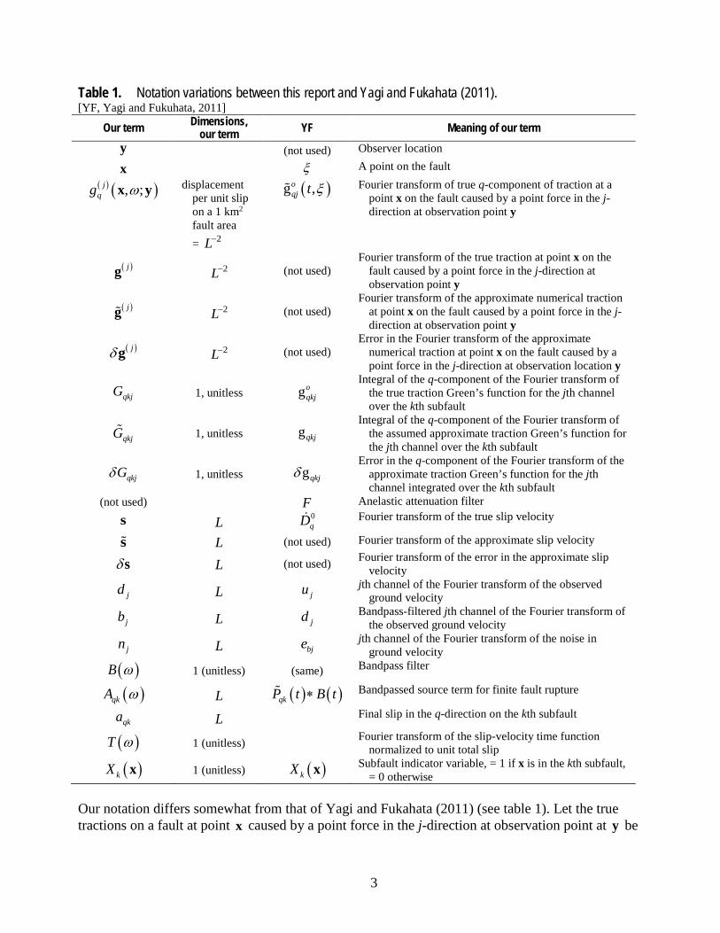
Table 1. Notation variations between this report and Yagi and Fukahata (2011). [YF, Yagi and Fukuhata, 2011]

Our term Dimensions, our term YF Meaning of our term

y (not used) Observer location

x ξ A point on the fault ( ) ( ), ;jqg ωx y displacement

per unit slip on a 1 km2 fault area = 2L−

( )g ,oqj t ξ Fourier transform of true q-component of traction at a

point x on the fault caused by a point force in the j-direction at observation point y

( )jg 2L− (not used)

Fourier transform of the true traction at point x on the fault caused by a point force in the j-direction at observation point y

( )jg 2L− (not used) Fourier transform of the approximate numerical traction

at point x on the fault caused by a point force in the j-direction at observation point y

( )jδg 2L− (not used) Error in the Fourier transform of the approximate

numerical traction at point x on the fault caused by a point force in the j-direction at observation location y

qkjG 1, unitless goqkj

Integral of the q-component of the Fourier transform of the true traction Green’s function for the jth channel over the kth subfault

qkjG 1, unitless gqkj Integral of the q-component of the Fourier transform of

the assumed approximate traction Green’s function for the jth channel over the kth subfault

qkjGδ 1, unitless gqkjδ Error in the q-component of the Fourier transform of the

approximate traction Green’s function for the jth channel integrated over the kth subfault

(not used) F Anelastic attenuation filter

s L 0qD Fourier transform of the true slip velocity

s L (not used) Fourier transform of the approximate slip velocity

δs L (not used) Fourier transform of the error in the approximate slip velocity

jd L ju jth channel of the Fourier transform of the observed ground velocity

jb L jd Bandpass-filtered jth channel of the Fourier transform of the observed ground velocity

jn L bje jth channel of the Fourier transform of the noise in ground velocity

( )B ω 1 (unitless) (same) Bandpass filter

( )qkA ω L ( ) ( )qkP tt B∗ Bandpassed source term for finite fault rupture

qka L Final slip in the q-direction on the kth subfault

( )T ω 1 (unitless) Fourier transform of the slip-velocity time function normalized to unit total slip

( )kX x 1 (unitless) ( )kX x Subfault indicator variable, = 1 if x is in the kth subfault, = 0 otherwise

Our notation differs somewhat from that of Yagi and Fukahata (2011) (see table 1). Let the true tractions on a fault at point x caused by a point force in the j-direction at observation point at y be

4

( ) ( ), ; j ωg x y , its numerical approximation be ( ) ( ) ( ) ( ) ( ) ( )1 2, ; , ; , ;Tj j jg gω ω ω = g x y x y x y , and the error

in ( )jg be ( ) ( ), ;jδ ωg x y . Thus,

( ) ( ) ( ) ( ) ( ) ( ), ; , ; , ;j j jω ω δ ω= +g x y g x y g x y . (1.1)

Similarly, let the relation between the true slip-velocity distribution at point x , the modeled slip-velocity distribution, and the error in slip velocity be

( ) ( ) ( ), , ,ω ω δ ω= +s x s x s x . (1.2)

Then the ground velocity in the j-direction ( ),jd ω y is equal to the noise-free velocity ( ), jv ω y

plus the ground noise ( ),jn ω y :

( ) ( ) ( ), , ,jj jd v nω ω ω= +y y y . (1.3)

Combining these equations into the usual representation theorem, we obtain

( ) ( ) ( ) ( ) ( ), , , ; ,jj j

A

d dA nω ω ω ω∈

= +∫x

y s x g x y y (1.4)

( ) ( ) ( ) ( ) ( ),j j j jj

A A A A

dA dA dA dA nδ δ δ δ ω∈ ∈ ∈ ∈

= + + + +∫ ∫ ∫ ∫x x x x

s g s g s g s g y , (1.5)

where the dot operator is the usual vector dot product of two vectors, and where we have suppressed all the arguments for clarity.

Yagi and Fukahata (2011) do not explicitly write equation 1.5; instead, they assume no slip-velocity error—that when their inversion converges, it converges to the true slip-velocity model, and so

( ), 0δ ω =s x . In reality, their slip-velocity model is composed of constant-slip-velocity subfaults. Therefore, using non-infinitesimal subfaults, their slip-velocity model cannot converge to the true slip-velocity model, which is not included in the span of their constant-slip-velocity basis functions.

The assumption of no slip-velocity error enables Yagi and Fukahata (2011) to drop the terms in δs above, yielding:

( ) ( ) ( ) ( ) ( ) ( ) ( ) ( ), , , ; , , ; ,j jj j

A A

d dA dA nω ω ω ω δ ω ω∈ ∈

= + +∫ ∫x x

y s x g x y s x g x y y

. (1.6)

Combining terms and dropping all the arguments inside the integral for simplicity yields

( ) ( ) ( ) ( ), ,j jj j

A

d dA nω δ ω∈

= + + ∫x

y s g g y . (1.7)

We can increase the generality of this equation by letting the index j refer to the jth data channel, 1, 2 ,,j J= , where “channel” is defined as a single component of motion at a single observation point

y and there are J total channels. Then observation point y is subsumed into index j, and

5

( ) ( ) ( ) ( ) j jj j

A

d dA nω δ ω∈

= + + ∫x

s g g . (1.8)

Yagi and Fukahata (2011) assembled their slip model from K constant-slip-velocity subfaults:

( ) ( ) ( )1

, k

Ki t

qk kk

a T e Xωω ω −

=

= ∑s x x , (1.9)

where qka is the total (final) slip of the kth subfault in the orthogonal 1q = and 2q = directions on the

fault; ( )T ω is the Fourier spectrum of the slip-velocity time function normalized to unit total slip, assumed to be constant over each subfault; kt is the rupture time of the kth subfault, assumed to be constant over the subfault; and ( ) : 1kX =x if point x is in the kth subfault, : 0= otherwise.

Let the integral of a single component q of the approximate Green’s functions over the kth subfault be

( ) ( ) ( ) ( ) : , qkjG g X dAω ω∈

= ∫ x x

jq k

x A

, (1.10)

with a similar equation for the integral of ( )j

qδg . (Note that this integral is never evaluated.) Combining these last two relations into the preceding one,

( ) ( ) ( ) ( ) ( ) ki tj qk qkj qkj j

q k

d a T e G G nωω ω ω δ ω ω− = + + ∑∑ . (1.11)

Furthermore, assume that the data are filtered with some bandpass filter ( ).B ω Then the filtered data are given by

( ) ( ) ( ) ( ) ( ) ( ) ( ) ( ) ( )ki tj j qk qkj qkj j

q kGb B d a T e B G B nωω ω ω ω ω ω δ ω ω ω− = = + + ∑∑ . (1.12)

Define ( ) ( ) ( ) ( ) : ki tqkj qkjH T e B Gωω ω ω ω−= and ( ) ( ) ( ) : ki t

qk qkA a T B e ωω ω ω −= . Combining all these relations gives Yagi and Fukahata’s (2011) equation 7 in different notation:

( ) ( ) ( ) ( ) ( ) ( ) j qk qkj qk qkj jq k q k

b a A G B nHω ω ω δ ω ω ω= + +∑∑ ∑∑ . (1.13)

The first term on the right side of the equals sign is just the slip-velocity model “convolved” with the erroneous numerical Green’s function—in other words, it is the usual finite-fault forward synthetic in this type of inversion. Equation 1.13 can be rewritten

( ) ( ) ( ) ( ) ( ) P

j pj jpp

b A G B nω ω ω ω ω= +∑ , (1.14)

where the double sum over q and k has been replaced by a single sum over p, with 2P K= and where

( ) ( ) ( )pj pj pjG G Gω ω δ ω= + . (1.15)

6

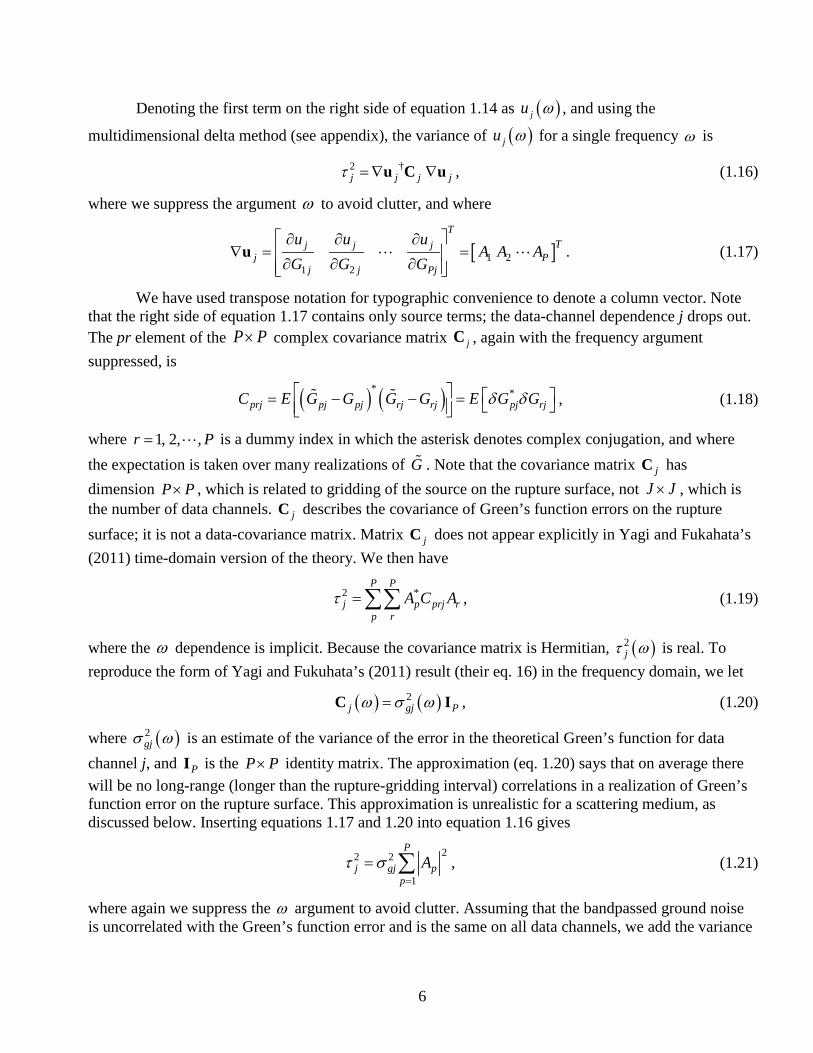
Denoting the first term on the right side of equation 1.14 as ( )ju ω , and using the

multidimensional delta method (see appendix), the variance of ( )ju ω for a single frequency ω is

2 †j j j jτ = ∇ ∇u C u , (1.16)

where we suppress the argument ω to avoid clutter, and where

[ ]1 21 2

TTj j j

j Pj j Pj

u u uA A A

G G G ∂ ∂ ∂

∇ = = ∂ ∂ ∂

u . (1.17)

We have used transpose notation for typographic convenience to denote a column vector. Note that the right side of equation 1.17 contains only source terms; the data-channel dependence j drops out. The pr element of the P P× complex covariance matrix jC , again with the frequency argument suppressed, is

( ) ( )* *prj pj pj rj rj pj rjC E G G G G E G Gδ δ = − − =

, (1.18)

where 1, 2, ,r P= is a dummy index in which the asterisk denotes complex conjugation, and where the expectation is taken over many realizations of G . Note that the covariance matrix jC has dimension P P× , which is related to gridding of the source on the rupture surface, not J J× , which is the number of data channels. jC describes the covariance of Green’s function errors on the rupture surface; it is not a data-covariance matrix. Matrix jC does not appear explicitly in Yagi and Fukahata’s (2011) time-domain version of the theory. We then have

2 *P P

j p prj rp r

A C Aτ =∑∑ , (1.19)

where the ω dependence is implicit. Because the covariance matrix is Hermitian, ( )2jτ ω is real. To

reproduce the form of Yagi and Fukuhata’s (2011) result (their eq. 16) in the frequency domain, we let

( ) ( )2j gj Pω σ ω=C I , (1.20)

where ( )2gjσ ω is an estimate of the variance of the error in the theoretical Green’s function for data

channel j, and PI is the P P× identity matrix. The approximation (eq. 1.20) says that on average there will be no long-range (longer than the rupture-gridding interval) correlations in a realization of Green’s function error on the rupture surface. This approximation is unrealistic for a scattering medium, as discussed below. Inserting equations 1.17 and 1.20 into equation 1.16 gives

22 2

1

P

j gj pp

Aτ σ=

= ∑ , (1.21)

where again we suppress the ω argument to avoid clutter. Assuming that the bandpassed ground noise is uncorrelated with the Green’s function error and is the same on all data channels, we add the variance

7

2bσ of the ground noise to equation 1.21 to obtain the final frequency-domain analog of Yagi and

Fukahata’s (2011) equation 16:

( ) ( ) ( ) ( )22 2 2

1

P

j gj p bp

Aτ ω σ ω ω σ ω=

= +∑ . (1.22)

Equation 1.22 tells us that the variance of the computed ground motion has one component caused by uncertainty in the Green’s functions and another component caused by the usual ground and instrumental noise. Note the distinction between the frequency-domain result and Yagi and Fukahata’s time-domain result; in the frequency domain, all frequencies decouple, and so our result (eq. 1.22) is the diagonal element of the data-covariance matrix, whereas Yagi and Fukahata’s equation 16 yields a time-domain data-covariance matrix with nonzero off-diagonal elements.

The Continuous-Integral Case

Yagi and Fukahata (2011) pose their result in terms of constant-slip subfaults, and so the generalization to a continuous spatial variation of the slip function is straightforward. We express the slip velocity function as

( ) ( ) ( ) ( )( )2

1

ˆ, , expq qq

a T i tω ω ω=

= −∑s x e x xx , (2.1)

where 1q = and 2q = are the strike-slip and dip-slip components, respectively; ( )t x is the time at which rupture initiates at point x; and ˆqe is a unit vector in the q-direction. Note that in this formulation, rake does not rotate over time at point x. The final result (eq. 2.8) does not depend on this parameterization of the source. From equation 1.8 we have

( ) ( ) ( ) jj j

A

d dA nω ω∈

= +∫x

s g , (2.2)

and the 2 2× covariance matrix of the Green’s function error for the jth data channel is

( ) ( ) ( ) ( )( )

( ) ( )*

1*1 2

2

, , , ,j

j jj j T jj

gE E g g

g

δω δ ω δ ω δ δ

δ

= =

xC x y g x g y y y

x. (2.3)

This result is obtained because the mean of the Green’s function errors is assumed to be zero (the theoretical Green’s functions are assumed to not have long-wavelength biases), and inspection of the actual data show them to have a mean that is essentially zero, as we show later. Then

( ) ( ) ( ) ( )2 † , , , ,jj

A A

d dτ ω ω ω ω⊂ ⊂

= ∫ ∫x y

s x C x y s y x y , (2.4)

where A is the fault surface. In this multiple integral, x and y are dummy variables of integration over the fault surface, and y is unrelated to channel j. Physically, we might expect two different functional forms for the spatial covariance. If it is dominated by finite frequency effects, we might expect that an element of the covariance of the Green’s function errors might take the form

8

( ) ( ), ,j fω ω β∝ −C x y x y , (2.5)

where β is the shear-wave speed of the medium and f is a decreasing function such as a Gaussian function centered at the origin. We expect scaling to be related to the shear-wave speed because the S wave is typically much stronger than the P wave in finite-source seismograms. In such a model, errors in the Green’s functions would be correlated at progressively longer distances as the wavelengths of the shear wave increased. However, if the Green’s functions errors are related to unmodeled spatial variations in rigidity along the fault surface, this function might have no frequency dependence and would have the same form as the covariance of rigidity along the fault.

Expanding equation 2.4, we have

( ) ( ) ( ) ( ) ( )( )

12 * *1 2

2,j

jA A

ss s d d

sτ ω

⊂ ⊂

=

∫ ∫

x y

yx x C x y x y

y, (2.6)

where

( ) ( ) ( ) ( ) ( )( ) ( ) ( ) ( )

* *1 1 1 2

* *2 1 2 2

, ,j j j j

jj j j j

g g g gE

g g g g

δ δ δ δω

δ δ δ δ

=

x y x yC x y

x y x y. (2.7)

In these equations, ω dependence of the right-hand terms is implied. Equation 2.4 is the general result, but we can simplify it for the common case that the rake in an earthquake rupture is primarily unidirectional. We can further simplify it by choosing the unit vector 1e to be directed along the dominant slip direction and assuming that the other component of slip is negligible, which is true for the 2009 L’Aquila, Italy, earthquake. We further assume that the 1e component of Green’s function error is

uncorrelated with the 2e component, and so jC becomes diagonal; finally,

( ) ( ) ( ) ( )2 *1 111, , , ,j

jA A

s C s d dτ ω ω ω ω⊂ ⊂

= ∫ ∫x y

x x y y x y . (2.8)

To the best of our knowledge, equations 2.4 to 2.8 are new results, not obtained elsewhere. There are two major differences between our results and those of previous workers: (1) equations 2.4 and 2.8 explicitly use the spatial-covariance function ( ), ,j ωC x y , which is absent in Yagi and Fukahata’s (2011) model; and (2) as shown below, we used observed empirical Green’s functions to evaluate the covariance function ( ), ,j ωC x y , rather than using theoretical considerations.

In considering the differences between the true traction Green’s function ( ) ( ),j ωg x and its

theoretical approximation ( ) ( ),j ωg x , we expect that the theoretical approximation is obtained in some simplified Earth model and that the real Earth structure is equal to the theoretical structure plus some random heterogeneities. If a mainshock fault zone has an extensive low-velocity zone, we assume that this feature is included in the theoretical traction functions ( ) ( ),j ωg x .The position vector x is a vector in three-dimensional space—that is, we are not assuming that our mainshock rupture is located on a two-dimensional surface (although the aftershocks we use define a fairly planar structure). We are examining the variation in the traction wavefield in the mainshock source volume.

9

Any traveltime and amplitude variations between ( ) ( ),j ωg x and ( ) ( ),j ωg x will depend on the wavenumber spectrum of the heterogeneities. Frankel and Clayton (1986) studied these variations in spatially stationary random media with Gaussian and exponential spatial-correlation functions and in a self-similar medium with equal variation of seismic velocity over a broad range of length scales. Because their assumed random media were spatially stationary, their covariance functions were functions of spatial separation only. (Note that even though these random media had different spatial-correlation functions, the amplitude distribution of the velocity perturbations was Gaussian.) They concluded that random media with self-similar velocity fluctuations with a correlation length of a = 10 km can explain both teleseismic traveltime anomalies and the presence of seismic coda at high frequencies. Each of these three types of media has its own correlation function, as plotted in figure 1.

Figure 1. Plot of three covariance functions for heterogeneous velocity-structure models. Normalizations are somewhat arbitrary; only shapes of curves are significant.

The exponential and Gaussian covariance functions are normalized to unit amplitude at zero separation, and the Von Karman correlation function is proportional to the Bessel function ( )0K r a ,

where r is the separation, arbitrarily normalized to ( )0 1 10 1K = in figure 1. ( ( )0 0K = ∞ .) Even for the self-similar heterogeneity spectrum, some nonzero covariance is expected at r = 10 km. Given a particular heterogeneity spectrum, we expect some spatially correlated traveltime and amplitude variations in the Green’s functions. If we consider the covariance of the true traction Green’s function

( ) ( ),j ωg x and its theoretical approximation ( ) ( ),j ωg x , we expect that there will be some nonzero covariance between different frequencies to account for traveltime errors, some evidence of which is presented below.

Note that Frankel and Clayton (1986) specified the covariance of their random seismic-velocity structures and that their variations in wave amplitude were the result of these random structures,

10

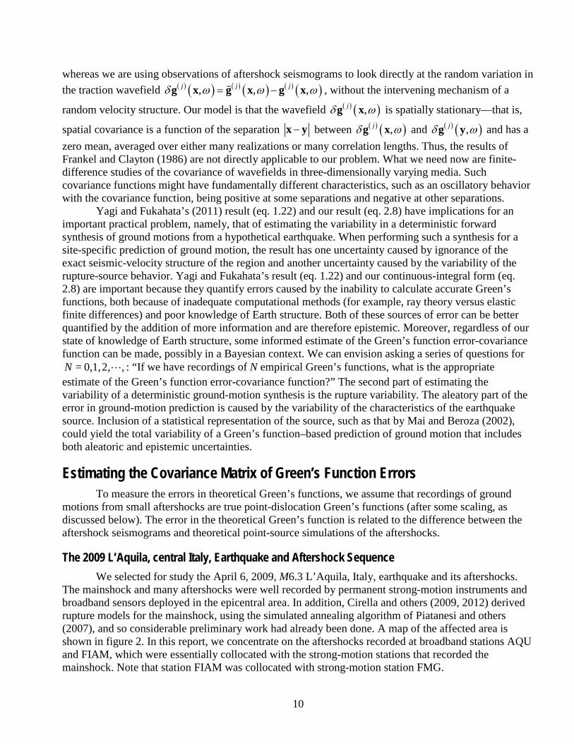
whereas we are using observations of aftershock seismograms to look directly at the random variation in the traction wavefield ( ) ( ) ( ) ( ) ( ) ( ), , ,j j jδ ω ω ω= −g x g x g x , without the intervening mechanism of a

random velocity structure. Our model is that the wavefield ( ) ( ),jδ ωg x is spatially stationary—that is,

spatial covariance is a function of the separation −x y between ( ) ( ),jδ ωg x and ( ) ( ),jδ ωg y and has a zero mean, averaged over either many realizations or many correlation lengths. Thus, the results of Frankel and Clayton (1986) are not directly applicable to our problem. What we need now are finite-difference studies of the covariance of wavefields in three-dimensionally varying media. Such covariance functions might have fundamentally different characteristics, such as an oscillatory behavior with the covariance function, being positive at some separations and negative at other separations.

Yagi and Fukahata’s (2011) result (eq. 1.22) and our result (eq. 2.8) have implications for an important practical problem, namely, that of estimating the variability in a deterministic forward synthesis of ground motions from a hypothetical earthquake. When performing such a synthesis for a site-specific prediction of ground motion, the result has one uncertainty caused by ignorance of the exact seismic-velocity structure of the region and another uncertainty caused by the variability of the rupture-source behavior. Yagi and Fukahata’s result (eq. 1.22) and our continuous-integral form (eq. 2.8) are important because they quantify errors caused by the inability to calculate accurate Green’s functions, both because of inadequate computational methods (for example, ray theory versus elastic finite differences) and poor knowledge of Earth structure. Both of these sources of error can be better quantified by the addition of more information and are therefore epistemic. Moreover, regardless of our state of knowledge of Earth structure, some informed estimate of the Green’s function error-covariance function can be made, possibly in a Bayesian context. We can envision asking a series of questions for

= 0,1,2, ,N : “If we have recordings of N empirical Green’s functions, what is the appropriate estimate of the Green’s function error-covariance function?” The second part of estimating the variability of a deterministic ground-motion synthesis is the rupture variability. The aleatory part of the error in ground-motion prediction is caused by the variability of the characteristics of the earthquake source. Inclusion of a statistical representation of the source, such as that by Mai and Beroza (2002), could yield the total variability of a Green’s function–based prediction of ground motion that includes both aleatoric and epistemic uncertainties.

Estimating the Covariance Matrix of Green’s Function Errors To measure the errors in theoretical Green’s functions, we assume that recordings of ground

motions from small aftershocks are true point-dislocation Green’s functions (after some scaling, as discussed below). The error in the theoretical Green’s function is related to the difference between the aftershock seismograms and theoretical point-source simulations of the aftershocks.

The 2009 L’Aquila, central Italy, Earthquake and Aftershock Sequence We selected for study the April 6, 2009, M6.3 L’Aquila, Italy, earthquake and its aftershocks.

The mainshock and many aftershocks were well recorded by permanent strong-motion instruments and broadband sensors deployed in the epicentral area. In addition, Cirella and others (2009, 2012) derived rupture models for the mainshock, using the simulated annealing algorithm of Piatanesi and others (2007), and so considerable preliminary work had already been done. A map of the affected area is shown in figure 2. In this report, we concentrate on the aftershocks recorded at broadband stations AQU and FIAM, which were essentially collocated with the strong-motion stations that recorded the mainshock. Note that station FIAM was collocated with strong-motion station FMG.

11

Figure 2. Map of the L’Aquila, Italy, region, modified from Cirella and others (2009). Red box, vertical projection of assumed fault-rupture area; red star, epicenter; black triangles, selected permanent strong-motion stations; open circles, broadband stations; blue dots, GPS stations; white dots, continuous GPS stations. Rupture surface dips 54° to the southwest.

We selected a set of 41 aftershocks recorded at station AQU (fig. 3) that had focal mechanisms within 30° of the mainshock mechanism and corner frequencies greater than 2.68 Hz.

12

Figure 3. Map of the L’Aquila, Italy, area showing focal mechanisms of 41 selected aftershocks.

Because our highest frequency of interest was 0.5 Hz, these events were point sources to a good approximation. A total of 33 of these aftershocks were recorded at station FIAM. Theoretical traction Green’s functions were calculated for them using the frequency-wavenumber integration method (Saikia, 1994, implemented in the TDMT software of Dreger, 2003) for two different seismic-velocity structures (realizations): the CIA model of Herrmann and others (2011), which was used by Cirella and others (2012) for station FMG; or the receiver-function (RF) model of Bianchi and others (2010), which was used for station AQU. Data-synthetic comparisons for these stations and aftershocks are plotted in figures 4–7. We removed from the analysis those data for which the observations had obvious ground-noise or processing glitches, namely events 72, 76, 83, and 85 for station AQU, leaving 37 events, and events 12, 15, 18, 24, 25, 27, and 31 for station FIAM, leaving 27 events.

13

Figure 4. Plots of observed aftershock ground velocity (red) and synthetic velocity (blue) for aftershocks 02–52, plotted at same scale as observations, for receiver-function velocity structure at station AQU. Number is peak velocity of data seismogram. First 40 seconds of total 60-second seismograms are plotted.

14

Figure 5. Plots of observed aftershock ground velocity (red) and synthetic velocity (blue) for aftershocks 53–87, plotted at same scale as observations, for receiver-function velocity structure at station AQU. Values are peak velocities of data seismogram. First 40 seconds of total 60-second seismograms are plotted.

15

Figure 6. Plots of observed aftershock ground velocity (red) and synthetic velocity (blue) for aftershocks 01–20, plotted at same scale as observations, for CIA velocity structure at station FIAM. Values are peak velocities of data seismogram. First 40 seconds of total 60-second seismograms are plotted.

16

Figure 7. Plots of observed aftershock ground velocity (red) and synthetic velocity (blue) for aftershocks 21–33, plotted at same scale as observations, for CIA velocity structure at station FIAM. Values are peak velocity of data seismogram. First 40 seconds of total 60-second seismograms are plotted.

Recovering Tractions from Ground Velocity We consider the relation between the units of our aftershock seismograms and the units of the

Fourier transform of a traction Green’s function. From the representation theorem,

( ) ( ) ( )( ), , , ;kk

A

v dAω ω ω∈

= ∫∫x

y s x g x y , (3.1)

where the Fourier transform of the kth-component of ground velocity ( ),kv ωy at point y and angular

frequency ω equals the integral over rupture area A of the Fourier transform ( ),ωs x of the slip-

velocity vector dotted with the Fourier transform ( )( ) , ;k ωg x y of the Green’s function for vector traction on a rupture surface, caused by an impulsive point force applied in the k-direction at point y. Let ( )*D be the dimensions of, for example, distance d, time t, force f, and so on and let ( )*U be the units

of, for example, meters, seconds, and so on:

( ) ( ) ( ) ( )dD v t D D D dAt

= =

s g , (3.2)

17

2d traction tt dt impulse

× =

. (3.3)

Now

( )2

21( )

f d tD

ft d= =g , (3.4)

where all of the physical quantities above are understood to be Fourier transforms. The units of the Fourier transform of ground velocity divided by the aftershock moment are inverse newtons:

1o

vU M N =

. (3.5)

We scale by the medium rigidity ( )µ x to get the units of the Fourier transform of ground per 1 m/s of slip on a 1-m2 rupture surface:

2

2

o

v N mU mM N

µ − = =

, (3.6)

in agreement with the dimensions of the traction Green’s functions. Below, when we refer to scaled ground velocity, we mean ground velocity multiplied by µ and divided by oM . This scaled ground velocity can equivalently be thought of as an “empirical traction.” Because oM is typically very large and ground velocities are small, we normalize the aftershock ground velocities by the factor

6 2

2101o

mM kmµ , (3.7)

which yields the Fourier transform of ground velocity per 1 m/s of slip on a 1-km2 rupture surface:

6 2

22

101o

v mU kmM km

µ − =

. (3.8)

The units of this scaled ground velocity are identical to those of the Fourier transform of the traction Green’s functions and so are identical to the units of the errors in the traction Green’s functions. For this reason, the units of the covariance of the errors in traction Green’s functions are km-4(!).

Our observations in this section are differences between the Fourier transforms of aftershock ground velocities and synthetic ground velocities calculated by using an assumed seismic-velocity structure and the aftershock’s seismic moment. Specifically, let index i be the aftershock index,

1, 2, ai n= , where an is the number of aftershocks, and index j indicates the jth realization of a random variable (the error associated with the jth erroneous velocity structure). For each frequency and component of motion we form the complex difference

j ji i id s∆ = − , (3.9)

18

where

ii i

i

Md gµ

= (3.10)

is the observed aftershock datum, which is a product of rigidity at the aftershock depth, the aftershock’s true moment iM and its true traction Green’s function ig . We also implicitly assume that the above equations apply separately to both the real and imaginary components of the complex quantities, so that when we write id we mean ( )Re id or ( )Im id . Let j

iM be our jth incorrect estimate of i iM µ (we

have absorbed the rigidity into jiM , the seismic potency) and let j

ig be our jth incorrect synthetic traction. The incorrect moments might come from different sources—for example, a moment-tensor solution using broadband data, or a long-period spectral level from a 2-Hz geophone—and the incorrect traction Green’s functions might come from different velocity structures. Then our synthetic aftershock seismogram is

j j ji i is M g=

, (3.11)

and (the real or imaginary part of) our complex difference is

j j j ji i i i i id s d M g∆ = − = −

. (3.12)

Normalizing by seismic moment and rigidity yields a quantity with the units of the traction Green’s function, namely the scaled complex difference (or, equivalently, the empirical traction)

ˆ j j j jii i i ij

i

dM g

M∆ = ∆ = −

. (3.13)

We can use our scaled complex differences to determine whether the CIA or the RF model is better at station AQU. The scaled complex differences in the complex plane for station AQU, using the CIA model and RF velocity models, are plotted in figures 8 and 9, respectively. These figures show that the scaled complex differences grow in magnitude as frequency increases and that the CIA model is considerably better than the RF model (the CIA model having smaller complex differences) at station AQU. However, since Cirella and others (2009, 2012) used the RF model for station AQU, we continue to use that model for station AQU. For many aftershocks, the complex differences form expanding helices, corresponding to progressive phase shifts as a function of frequency caused by time mismatches between the synthetic and real seismograms, which is evidence of nonzero covariance of Green’s function errors at differing frequencies.

19

Figure 8. Argand plot of complex differences between real and synthetic ground velocities as a function of frequency at station AQU, using CIA model. Datum color is proportional to frequency. Colored dots showing complex difference data for a particular aftershock are connected with a black line.

Figure 9. Argand plot of complex differences between real and synthetic ground velocities as a function of frequency at station AQU, using receiver-function model. Datum color is proportional to frequency. Colored dots showing complex difference data for a particular aftershock are connected with a black line.

20

Covariance as a Function of Separation on the Fault

To determine the variance ( )2j nτ ω ,we need the spatial-covariance matrix from equation 2.8,

( )11 , ,ji k nC ωx x , where j is the channel number (a single component of motion at a single station), ix

and kx are two points on the fault (here, aftershock locations), and the subscript “11” indicates the covariance of the Green’s function error in the “1”-direction (taken to be the dominant direction of mainshock slip) at point ix with the Green’s function error in the “1”-direction at kx . Including the

index on ω , ( )11 , ,ji k nC ωx x has six indices. For notational simplicity, we suppress some of these

indices by defining a new spatial-covariance matrix

( ) ( ) ( ) ( ) ( ) ( )* *11 1 1

ˆ ˆ, , , , , ,j j j jn i k n i n k n i n k nikK C E g g Eω ω δ ω δ ω ω ω = = = ∆ ∆ x x x x x x , (3.14)

where we omit the slip-direction indices entirely because the aftershock rakes are chosen to be within 30° of the dominant slip direction. The term ( )ˆ ,i nω∆ x is the rigidity- and moment-scaled complex difference (or empirical traction) introduced earlier. We have previously speculated that the covariance would be a function of separation of the aftershocks, ik i kr = −x x . Individual values of

( ) ( )( )*ˆ ˆRe , ,i n k nE ω ω ∆ ∆ x x (which we refer to as a “covariance datum”) as a function of ikr are

plotted in figure 10 (blue plus signs), where the expectation is taken by averaging the result for each i-k pair over three components of motion and three values of n corresponding to three adjacent Fourier components in the frequency band 0.2667–0.300 Hz. Because the data and theoretical Green’s functions have a 60-s duration, there are a total of 30 frequency components with a frequency interval of 1/60 s = 0.01667 Hz. For the 37 events recorded at station AQU, there are 703 non-redundant i-k pairs and 703 blue plus signs plotted in figure 10 for AQU.

To obtain the expected values, we should further average the covariance data within distance bins. However, because the perturbations of the covariance data values caused by moment errors are skewed (because a moment error of a factor of 2 doubles some data while only halving other data), numerical tests of the effect of moment errors (not shown here) indicate that the covariance function inferred from the median of the covariance data is largely unbiased, whereas the mean of the covariance data is systematically biased high. For both stations AQU and FIAM we divided the distance range into 10 bins, with the width of each distance bin adjusted to hold the same number (~70) of covariance data. To estimate the covariance as a function of separation, we used the median of the covariance data in each distance bin (fig. 10).

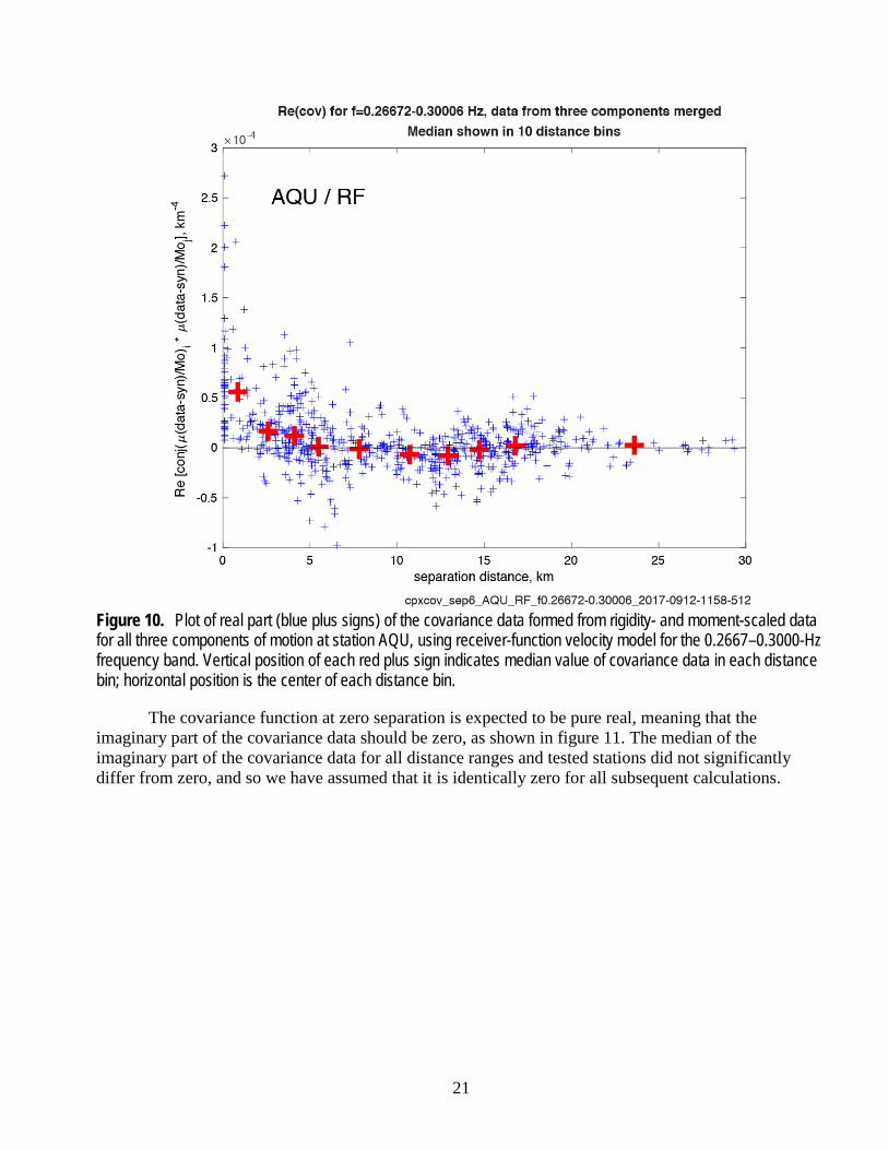
21

Figure 10. Plot of real part (blue plus signs) of the covariance data formed from rigidity- and moment-scaled data for all three components of motion at station AQU, using receiver-function velocity model for the 0.2667–0.3000-Hz frequency band. Vertical position of each red plus sign indicates median value of covariance data in each distance bin; horizontal position is the center of each distance bin.

The covariance function at zero separation is expected to be pure real, meaning that the imaginary part of the covariance data should be zero, as shown in figure 11. The median of the imaginary part of the covariance data for all distance ranges and tested stations did not significantly differ from zero, and so we have assumed that it is identically zero for all subsequent calculations.

22

Figure 11. Plot of imaginary part (blue plus signs) of covariance data formed from rigidity- and moment-scaled data for all three components of motion at station AQU, using receiver-function velocity model for the 0.2667–0.3000-Hz frequency band. Vertical position of each red plus signs indicates median value of covariance data in each distance bin; horizontal position is center of each distance bin. Median of imaginary part of covariance data at small separation is approximately zero, as expected.

The median covariance function for the data from all components of motion in 10 frequency bands at station AQU is plotted in figure 12.

23

Figure 12. Plot of median covariance as a function of separation distance in 10 frequency bands for station AQU, using receiver-function velocity model and lumping data from all components of motion together.

Surprisingly, if we normalize all these curves to unit amplitude at zero separation, we see varying behaviors with frequency for the AQU/RF covariance data and the FIAM/CIA data. For station AQU there is a conspicuous variation in the coherence functions with frequency, visible as the high-frequency covariance functions lying below the dashed average and the low-frequency data lying above the dashed average in figure 13, vaguely consistent with the behavior predicted in equation 2.5; however, no frequency dependence is evident in figure 13 for station FIAM. Because the source zone for the aftershocks recorded at stations AQU and FIAM is the same, it is difficult to identify a physical mechanism that would produce the various frequency behaviors.

24

Figure 13. Plot of median covariance at station AQU as a function of separation distance for 10 frequency bands, lumping all components of motion together and normalizing to unit amplitude at smallest separation. Dashed curve, average of all solid curves. Note that there is a clear systematic variation of curves with frequency.

25

Figure 14. Plot of median covariance at station FIAM as a function of separation distance for 10 frequency bands, lumping all components of motion together and normalizing to unit amplitude at the smallest separation. Dashed curve, average of all solid curves. Note that there is no clear systematic variation of curves with frequency.

The dashed average covariance functions in figures 13 and 14 are similar in shape to Frankel and Clayton’s (1986) covariance functions for exponential and self-similar media shown in figure 1, although our covariance functions indicate a smaller covariance distance than their 10 km, suggesting the way to approach the theory-error problem in ground-motion inversions is to treat the problem as one of waves in random media.

A Covariance Model The covariance functions for the three components of motion at station AQU differ

systematically. We have sought to create a simple parameterization of these covariances that preserves

26

the component differences. We are developing this continuous empirical covariance function to insert into equation 2.8 in place of the discretized term ( )j

ik nK ω in equation 3.14. At this point, we need to separate the dependence on the station s from the dependence on component of motion c. We parameterize the covariance as a continuous function of r and ω as

( ) ( ) ( ), ,sc sc sK r N rω ω ω=Ω , (3.15)

where ( ),sN r ω for station FIAM is the frequency-independent average correlation function (dashed

curve, of figure 14) normalized to unit amplitude at zero separation, and ( ) , 1, 2,or 3sc cωΩ = , AQU or FIAMs = , is the covariance at minimum separation of the c component of motion at station s

as a function of frequency. To calculate ( )sc ωΩ , we applied the same analysis as in figure 10 to individual components of motion, this time in three frequency bands with a bandwidth of 0.1667 Hz consisting of 10 Fourier components each (fig. 15), with center frequencies of 0.0917, 0.2584, and 0.4251 Hz. The piecewise linear curves in figure 15 were used to interpolate the value of ( )sc ωΩ at

frequencies between those at which ( )sc ωΩ was measured (circles, triangles, and crosses). For station AQU, because its covariance functions showed a systematic variation with frequency that we wanted to preserve, the individual colored piecewise linear functions in figure 13 were used for ( ),sN r ω . Unfortunately, we do not have a smooth theoretical model of the expected behavior of these curves

( ),sN r ω , and each curve is less well defined than the dashed average curve, so we expect that the ultimate effect of using these frequency-dependent curves will be to make the frequency dependence of the resulting ( )2τ ω somewhat irregular.

27

Figure 15. Plot of covariance at zero separation for various combinations of component and frequency bands for three components of motion at stations AQU and FIAM. Measured values of ( )sc ωΩ are shown by circles, triangles, and crosses. Piecewise linear functions are interpolants.

Epistemic Error of Finite-Source Synthetic Seismograms With this parameterization we now have everything we need to estimate the epistemic error of

our finite-source synthetic seismograms. Equation 2.8 becomes

( ) ( ) ( ) ( )2 *1 1, , ,sc

scA A

s K r s d dτ ω ω ω ω⊂ ⊂

= ∫ ∫x y

x y x y , (3.16)

where r = −x y .

For the rupture model ( )1 ,s ωy we use the (unpublished) best fitting model of Cirella and others (2009), shown in figure 16. Note that this is not their average model from ensemble inference. If the model ( )1 ,s ωx has the correct moment and moment rate, the smoothing effects of the integral (eq.

3.16) may make the estimate of ( )2scτ ω relatively insensitive to the exact slip velocity model used.

28

Alternatively, we might be able to use the rupture model with the least moment. We speculate, but have not proved, that this rupture model would give the smallest possible estimate of ( )2

scτ ω .

Figure 16. Best fitting L’Aquila mainshock-rupture model. Colors show peak slip velocity, solid white contours show rupture time, dashed contours show parameter “acceleration time” Tacc in Yoffe slip function of Tinti and others (2005), and black arrows show direction of slip.

Because r = −x y , equation 3.16 is a spatial convolution over x (or y ), performed using a two-dimensional Fourier transform, followed by a simple area integral over the other integration variable. We have verified numerically that the estimates of ( )2

scτ ω obtained from equation 3.16 agree very well with the variance of an ensemble of ground motions calculated from an ensemble of δg having a given covariance function. Derived values of ( )scτ ω are plotted in figures 17 and 18 for station AQU, using the RF velocity structure, and in figure 19 for station FIAM, using the CIA velocity structure.

29

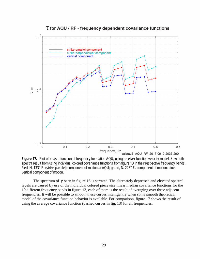
Figure 17. Plot of τ as a function of frequency for station AQU, using receiver-function velocity model. Sawtooth spectra result from using individual colored covariance functions from figure 13 in their respective frequency bands. Red, N. 133° E. (strike-parallel) component of motion at AQU; green, N. 223° E. component of motion; blue, vertical component of motion.

The spectrum of seen in figure 16 is serrated. The alternately depressed and elevated spectral levels are caused by use of the individual colored piecewise linear median covariance functions for the 10 different frequency bands in figure 13, each of them is the result of averaging over three adjacent frequencies. It will be possible to smooth these curves intelligently when some smooth theoretical model of the covariance function behavior is available. For comparison, figure 17 shows the result of using the average covariance function (dashed curves in fig. 13) for all frequencies.

30

Figure 18. Plot of τ as a function of frequency for station AQU, using receiver-function velocity structure. Smooth spectra result from using dashed average covariance function in figure 13. Red, N. 133° E. (strike-parallel) component of motion at station AQU; green, N. 223° E. component of motion; blue, vertical component of motion.

31

Figure 19. Plot of τ as a function of frequency for station FIAM, using CIA velocity structure. Red, N. 133° E. (strike-parallel) component of motion at station FIAM; green, N. 223° E. component of motion; blue, vertical component of motion

Use of Epistemic Ground-motion Variance 2τ in a Simulated Annealing Inversion Rather than seeking the “best fitting” rupture model, we instead seek to find two rupture models

that fit the data within the error bounds given by 2τ , by using a chi-squared test, as described later. The two models we find are those which minimize and maximize some desired property of the rupture models. By finding these two models we set hard bounds on the value of the desired property. The specific property that we wish to investigate is the correlation between rupture-model parameters, such as peak slip velocity and rupture velocity, in models of real earthquakes. Piatanesi and others’s (2007) inversion’s “cost” function can be modified to find rupture models with high or low degrees of correlation between pairs of rupture parameters.

A Cost Function Related to chi-squared We modify the Piatanesi and others (2007) cost function in two ways. The first is to use a chi-

squared test to make the cost low for rupture models that fit the data within the theoretical errors 2τ . Let

32

( )mjv ω be the synthetic ground velocity at frequency ω for the jth data channel and the mth trial rupture model ms .

( ) ( ) ( ) ( ), ,jmj m

A

v dAω ω ω∈

= ∫x

s x xg , (4.1)

and let the error in this synthetic motion be ( ) ( ) ( )mj j mje d vω ω ω= − .

Our first goal is to define a cost function that is minimized for any model whose errors ( )mjv ω

are comparable to ( )jτ ω . A chi-squared test is well suited to determine this cost function. We form variable

( ) ( )2J K

m mj k j kj k

eχ ω τ ω= ∑∑ , (4.2)

where we now recognize that our calculations use discrete frequencies , 1, 2, ,k k Kω = . Because we divide by ( )jτ ω , we must set a floor under it to avoid dividing by small numbers. The total number of observations is O J K= × (recalling that the jth data channel is a single component at a single station), and the total number of model parameters is 3M = × (number of nodes in the rupture model), and so the number of degrees of freedom is D O M= − . Because rake is fixed to the dominant slip rake, there are only three unknowns per node: peak slip velocity, rupture time, and the parameter “acceleration time” Tacc in the Yoffe slip function of Tinti and others (2005), which governs the slip-rate time function for each point on the rupture. We calculate ( )22, 2mp D χ , where p is the regularized incomplete gamma

function (Press and others, 1986, p. 160–161, 706). We form ( )21 2, 2m mq p D χ= − . Actual misfits

( )mj ke ω are significantly different from theoretical misfits ( )j kτ ω if mq is near 0 or 1. More specifically, if N realizations of a set of L observed residuals of unit standard deviation are generated, and if the expected standard deviations are unity—that is, the observed residuals are consistent with the theoretical—and if q is calculated for all N realizations, q will be uniformly distributed in the interval [0,1], and ( )1 Q *100− percent of the N realizations will have q > Q; (that is 5 percent of the N realizations will have q > 0.95), and 5 percent of the N realizations will have q < 0.05 (that is 10 percent of the N realizations will lie in the two outer 5 percent bands). This is a 10 percent rate of falsely saying the observed residuals are significantly different from the expected residuals. Therefore, it is probably wise not to say the observed residuals are significantly different from the expected residuals unless q > 0.99 or q < 0.01. When the observed errors are significantly different from the expected errors, q can easily be 0.000001 or 0.999999.

We want to create a cost function that is fairly low and flat for 0.1 0.9mq< < and rises sharply outside that band, so that a rupture model whose misfit differs strongly from the theoretical misfit is sharply penalized. For that reason, we create a cost function mΧ that is symmetrical about 0.5mq = . Let

1 12 2m md q= − − and ( ) 1 2m m mQ d d γ γ= − , where γ is a user-chosen parameter that controls the

steepness of the walls of the function. Then

33

( ) ( )( )min 0.005 ,1m m m mQ d QΧ = . (4.3)

( )m mqΧ for 0 1mq≤ ≤ and for three values of γ is plotted in figure 20.

Figure 20. Plot of X ( )m mq values for 0 1mq≤ ≤ and for three values of γ .

Cost Function Based on Correlation of Rupture Parameters The second cost component penalizes models having the least or greatest correlation between

desired pairs of rupture-model parameters, such as peak slip velocity and rupture velocity. We seek the two models having the greatest and least correlation as the end-member models, so that we are confident that all other rupture models will have intermediate correlations.

The correlation of two functions ( )r x and ( )s x defined over fault area A is

( )( ) ( )( )1

rsr sA

r r s sC d

A σ σ⊂

− −= ∫

x

x xx , (4.4)

where r and s are the mean values of r and s over area A, and

( )( )22 1r

A

r r dA

σ⊂

= −∫x

x x , (4.5)

with a similar equation for 2sσ . In the Piatanesi and others (2007) algorithm, the rupture parameters,

among them peak slip speed and rupture time, are defined at the nodes of a rectangular grid, and bilinear interpolation is used to define the parameters at points between the nodes. Analytic expressions are obtainable for the correlation of two rupture parameters defined in this way. However, we need to find the correlation of peak slip speed and rupture speed, which is the inverse of the magnitude of the

34

gradient of the rupture time. A simple analytic expression cannot be found for the correlation of a bilinear function and the inverse of the magnitude of the gradient of a bilinear function. For this reason, we approximated the bilinear functions defined on a rectangle by partitioning each rectangle into two triangles upon which the functions are linear. Though still involving tedious algebra, the correlations that we need can be analytically obtained on each triangle.

Denoting the peak slip speed of the mth model as ( )ˆms x and rupture speed as ( )mr x , we

calculate the correlation of the two, ( )ˆm

rsC , which can range from −1 to 1.

Combined Cost Function We define a combined cost function

( )ˆ , 1m

m m rsCεϑ ϑΛ = Χ − = ± . (4.6)

We choose 0 1ε< < so that the cost function primarily finds models that fit the data within the error bar. If we choose 1ϑ = + , models with a positive correlation between peak slip speed and rupture speed will be favored, whereas if we choose 1ϑ = − , models with a negative correlation between peak slip speed and rupture speed will be favored. Therefore, we run the simulated annealing algorithm twice, the first time with 1ϑ = + , and we find the model that fits the data and has the highest correlation of the two rupture parameters. We run the simulated annealing algorithm a second time with 1ϑ = − and find the model having the greatest anticorrelation between the two rupture parameters. This gives us bounds on the correlation of those parameters within which all models fitting the data must lie.

One of the advantages of the cost function in equation 4.6 is that it lies within the limited range 1mε ε− ≤ Λ ≤ + . Generally, when running a simulated annealing algorithm, the investigator knows

neither the global minimum value of the cost nor the approximate value of the cost on the “shoulders” of the global minimum. Using our cost function, the user has a very good idea of the critical temperature at which to run the algorithm in order to help it find the model having the global minimum cost.

Discussion Having detailed the derivation of our method, we now consider it in relation to Yagi and

Fukahata’s (2011) time-domain theory and other studies, most notably those by Bodin and others (2012), Duputel and others (2012), Dettmer and others (2014), and Minson and others (2014), all five of which used time-domain methods. The last four papers used Bayesian inference to derive a posterior PDF of model parameters. Yagi and Fukahata used a more traditional optimization technique; their equation 16 derived a time-domain data-covariance matrix that had the structure to be expected if there were errors in the theory—in other words, the matrix was not assumed to be diagonal. Their equation 16 showed that elements of the data-covariance matrix were proportional to the square of the slip amplitudes. They used two scalar hyperparameters to characterize the modeling error and the observation error, respectively, and they modified their values and the data-covariance matrix iteratively within a sequence of standard maximum-likelihood inversions.

In their time-domain Bayesian inference of a kinematic rupture model for the 2011 Tohoku, Japan, earthquake, Minson and others (2014) used a diagonal model-prediction covariance matrix, with elements having an amplitude equal to a fixed fraction of the largest datum squared, which serves as a proxy for the square of the slip amplitude in Yagi and Fukahata’s (2011) theory, and which they recognized as providing a better data-covariance matrix.

35

Two of these four studies were similar in developing the model-prediction covariance matrix iteratively as part of the Bayesian inference. Bodin and others (2012) expressed their modeling error in a model-prediction covariance matrix characterized by two hyperparameters, one for each of two different datasets, the posterior PDFs of which were estimated as part of the Bayesian inference of velocity structure in Australia. Dettmer and others (2014), who performed an inversion for the kinematic rupture parameters of the 2010 Maule, Chile, earthquake, derived their model-prediction covariance matrix by posterior analysis of the data-residual vector r . During the “burn-in” period, they derived the model-prediction covariance matrix iteratively by analysis of Trr . After burn-in, the covariance matrix was held constant; and at the end of the inference, the appropriateness of the covariance matrix was checked to guarantee its consistency with the original assumption of Gaussian residuals.

Duputel and others (2014) applied Bayesian inference to infer the static slip distribution from geodetic data in a vertically varying medium. As in several other studies, they updated their model-prediction covariance matrix during the inversion. In an interesting twist, however, they introduced a vector Ψ of Earth structure parameters (one-dimensional rigidity profile) and made their prediction covariance matrix linear in perturbations to Ψ by using a Born approximation. Their model-prediction covariance matrix was iteratively updated.

Our study differs from all of these others in three ways. (1) We explicitly accept that the seismic-velocity structure of the medium has random three-dimensional variations on all scales (many of them deterministically unknowable), leading to similar variations in Green’s function perturbations jδg . Thus, the most natural and general way to characterize these variations is through a statistical model for the spatial covariance ( ) ( ) ( )*, , , ,j j T jEω δ ω δ ω = C x y g x g y based on a combination of observations of empirical Green’s functions and theoretical studies, such as Frankel and Clayton (1986). (2) We use observed aftershock seismograms to derive an empirical spatial-covariance matrix that can be used to derive the variability of predicted large-rupture ground motions due to Green’s function uncertainty through equation 2.4 or 2.8. (3) Although Bayesian inference offers a complete solution to the problem of determining the posterior PDF of rupture-model parameters, it can require as many as 1010 forward kinematic simulations (Minson and others 2014). It might be that most interesting questions about some feature of rupture behavior (like average rupture speed) can be answered by finding three rupture models consistent with the covariance ( ), ,j ωC x y : the best-fitting rupture model, the model minimizing the feature, and the rupture model maximizing the feature, requiring only about 107 forward kinematic simulations.

Summary In this report, we have detailed a new approach for characterizing the effect of errors in

theoretical Green's functions during kinematic finite-fault inversion modeling. In particular, we have studied the effect of these erroneous Green's functions on the variance of synthetic ground velocity calculated by using rupture models of hypothetical earthquakes with extended rupture surfaces. The variance 2τ of the synthetic velocities is given by equation 2.4 in the particular case where slip rake varies over the rupture surface, and by equation 2.8 in the more usual case of relatively constant slip rake over the rupture surface. The variability of the Green's functions can be characterized by their spatial covariance on the rupture surface, given by equation 2.7. We suggest a method for determining this spatial covariance by a direct calculation of the errors in theoretical Green's functions. To measure the errors in theoretical Green’s functions, we assume that recordings of ground motions from small (point-source) earthquakes (typically, aftershocks) distributed on an extended rupture surface are true

36

point-dislocation Green’s functions after some scaling to units of traction (eq. 3.8). The errors in the theoretical Green’s functions are given by the differences between the small-earthquake seismograms and theoretical point-source simulations of the small earthquakes (eq. 3.13). We have calculated these differences for some aftershocks of the 2009 M6.1 L’Aquila, Italy, earthquake, using theoretical Green’s functions for two stations, AQU and FIAM (fig. 2), and two different seismic velocity structures (CIA and RF, figs. 4–7). From these differences, we calculate individual covariance data (eq. 3.14) and extract a covariance function as a function of separation distance and frequency (figs. 10–14) for each station. We combine these functions into a covariance model (eq. 3.15) (fig. 15) which we then use with a rupture model of a large earthquake (fig. 16) to calculate the expected variance 2τ of the ground velocities caused by errors in the theoretical Green's functions (figs. 17–19). We then propose to use these variances in an inversion for rupture behavior. Rather than seeking the rupture model that “best fits” the observed large-earthquake ground motions, we instead seek to find two rupture models that fit the data within the error bounds given by 2τ which may be done by using a chi-squared test (eq. 4.2). Two useful models are those that minimize and maximize some desired property of the rupture models. By finding these two models, we may be able to set hard bounds on the value of the desired property. Among all the potential properties, the specific property we wish to investigate is the correlation (eq. 4.4) between rupture-model parameters, such as peak slip velocity and rupture velocity, in models of real earthquakes. We propose a “cost function” (eq. 4.6) that can be used in a simulated annealing inversion algorithm to find the rupture models with the greatest and least correlation between peak slip velocity and rupture velocity consistent with the expected variance 2τ .

References Cited Aagaard, B.T., Graves, R.W., Schwartz, D.P., Ponce, D.A., and Graymer, R.W., 2010, Ground motion

modeling of Hayward Fault scenario earthquakes, Part I—Construction of the suite of scenarios: Bulletin of the Seismological Society of America, v. 100, p. 2927–2944, https://doi.org/10.1785/0120090324.

Bianchi, I., Chiarabba, C., and Piana Agostinetti, N., 2010, Control of the 2009 L’Aquila earthquake, central Italy, by a high-velocity structure—A receiver function study: Journal of Geophysical Research, v. 115, p. B12326, https://doi.org/10.1029/2009JB007087.

Bodin, T., Sambridge, M., Rawlinson, N., and Arroucau, P., 2012, Transdimensional tomography with unknown data noise: Geophysical Journal International, v. 189, n. 3, p. 1536–1556, https://doi.org/10.1111/j.1365-246X.2012.05414x.

Cirella, A., Piatanesi, A., Cocco, M., Tinti, E., Scognamiglio, L., Michelini, A., Lomax, A., and Boschi, E., 2009, Rupture history of the 2009 L’Aquila (Italy) earthquake from non-linear joint inversion of strong motion and GPS data: Geophysical Research Letters, v. 36, no. 19, L19304, https://doi.org/10.1029/2009GL039795.

Cirella, A., Piatanesi, A., Tinti, E., Chini, M., and Cocco, M., 2012, Complexity of the rupture process during the 2009 L’Aquila, Italy, earthquake. Geophysical Journal International, v. 190, p. 607–621, https://doi.org/10.1111/j.1365-246X.2012.05505.x.

Dettmer, J., Benavente, R., Cummins, P., and Sambridge, M., 2014, Trans-dimensional finite-fault inversion: Geophysical Journal International, v. 199, p. 735–751, https://doi.org/10.1093/gji/ggu280.

Dreger, D.S., 2003, TDMT_INV—Time domain seismic moment tensor inversion, in International Handbook of Earthquake and Engineering Seismology, Lee, W.H.K, Kanamori, H., Jennings, P.C., and Kisslinger, C., eds., Vol. B: London, Academic Press, 1627 p.

37

Duputel, Z., Rivera, L., Fukahata, Y., and Kanamori, H., 2012, Uncertainty estimations for seismic source inversions: Geophysical Journal International, v. 190, p. 1243–1256, https://doi.org/10.1111/j.1365-246X.2012.05554.x.

Frankel, A., and Clayton, R., 1986, Finite difference simulations of seismic scattering—Implications for the propagation of short period seismic waves in the crust and models of crustal heterogeneity: Journal of Geophysical Research, v. 91, p. 6465–6489.

Graves, R. and Pitarka, A., 2015, Refinements to the Graves and Pitarka (2010) broadband ground‐motion simulation method: Seismological Research Letters, v. 86, p.75–80.

Herrmann, R.B., Malagnini, L., and Munafò, I., 2011, Regional moment tensors of the 2009 L’Aquila earthquake sequence: Bulletin of the Seismological Society of America, v. 101, p. 975–993.

Mai, P.M., and Beroza, G.C., 2002, A spatial random field model to characterize complexity in earthquake slip: Journal of Geophysical Research, v. 107, p. ESE 10–1 – ESE 10–21, https://doi.org/10.1029/2001JB000588.

Minson, S., Simons, M., Beck, J.L., Ortega, F., Jiang, J., Owen, S.E., Moore, A.W., Inbal, A., and Sladen, A., 2014, Bayesian inversion for finite fault earthquake source models – II—The 2011 great Tohoku-oki, Japan earthquake, 2014: Geophysical Journal International, v. 198, p. 922–940, https://doi.org/10.1093/gji/ggu170.

Olson, A.H., and Apsel, R.J., 1982, Finite faults and inverse theory with applications to the 1979 Imperial Valley earthquake: Bulletin of the Seismological Society of America, v. 72, p. 1969–2001.

Papanicolaou, A., 2009, Taylor approximation and the delta method: Stanford University web page, accessed March 2, 2015, at http://web.standford.edu/class/cme308/OldWebsite/notes/TaylorAppDeltaMethod. [Not available March 30, 2017.]

Piatanesi, A., Cirella, A., Spudich, P., and Cocco, M., 2007, A global search inversion for earthquake kinematic rupture history—Application to the 2000 western Tottori, Japan earthquake: Journal of Geophysical Research, v. 112, https://doi.org/10.1029/2006JB004821.

Press, W.H., Flannery, B.P., Teukolsky, S.A., and Vetterling, W.T., 1986, Numerical recipes—The art of scientific computing: New York, Cambridge University Press, 818 p.

Saikia, C.K., 1994, Modified frequency-wavenumber algorithm for regional seismograms using Filon’s quadrature—Modelling of Lg waves in eastern North America: Geophysical Journal International, v. 118, p. 142–158.

Segall, P., and Du, Y., 1993, How similar were the 1934 and 1966 Parkfield earthquakes?: Journal of Geophysical Research, v. 98, p. 4527–4538.

Tinti, E., Fukuyama, E., Piatanesi, A., and Cocco, M., 2005, A kinematic source-time function compatible with earthquake dynamics: Bulletin of the Seismological Society of America, v. 95, p. 1211–1223.

Yagi, Y., and Fukahata, Y., 2011, Introduction of uncertainty of Green’s function into waveform inversion for seismic source processes: Geophysical Journal International, v. 186, p. 711–720.

38

Appendix 1. The Multidimensional Delta Method (MDM)

This review is based on online class notes (Papanicolaou, 2016). Define a P-element random vector [ ]1 2

TPX X X=X with means [ ]µ µ µ= 1 2

TPµ . We observe N (= 1 in our case)

independent random samples of the population of X and denote the samples ( ) ( ) ( )X X X

1 2 N .

The sample mean of pX is ( )

1

1ˆ , 1N

np p

nX X p P

N =

= =∑ and let X be the vector of sample

means. Consider a multivariate function ( )u X . A Taylor expansion about =X μ gives

( ) ( ) ( )( ) ( )ˆTu u u+ ∇ −X μ μ X μ . (5.1)

If this function has continuous partial derivatives, then

( ) ( )( ) ( )2ˆ 0,DN u u N τ− →X μ , (5.2)

where ( )20,N τ is the normal distribution with zero mean and variance 2τ , which is given by

( )( ) ( )2 Tu uτ = ∇ ∇μ C μ . (5.3)

The covariance matrix is a P P× matrix with elements

( )( )( ) ( )n nij i i j jC E X Xµ µ = − − , (5.4)

where the expectation is taken over the random realizations of X . In general, we do not know the true mean μ , and so we must approximate it by using X ; but in some cases (like ours, below), the gradient is identical whether evaluated at μ or X .

Application to the Ground-Motion Problem In these notes, we use a greatly simplified version of our ground-motion problem to

investigate the applicability of the MDM. Let

1

P

i ii

v s g=

=∑ , (5.5)

where =is ,i 1,2, P , is the slip speed on the ith subfault and ig is the approximate (that is,

theoretical) Green’s function evaluated on the ith subfault [ ]1 2T

Pg g g=g is a P element

random vector with true mean [ ]1 2T

Pg g g=g . Suppose that we have n independent random samples of the vector g (we might have calculated Green’s functions for n velocity structures); denote them by , =1,2, ,k ng

k . Define sample means (which differ from the true mean)

39

( )

1

1ˆn

k

kn =

= ∑g g . (5.6)

Then

( ) ( )( ) ( )2ˆ 0,Dn u u N τ− →g g , (5.7)

where the symbol “ D→” means “converges in the distribution”—in other words, the distribution of the quantity on the left-hand side approaches a normal distribution with zero mean and variance 2τ when many realizations of the left side are available. Note that there are realizations within realizations here. One realization of g is the mean of n realizations of g , and we need many realizations of g to verify that the distribution of the left side has variance 2τ , which is given by

2 ( ) ( )Tu uτ = ∇ ∇g C g

. (5.8)

Now

[ ]1 21 2

( )T

TP

P

u u uu s s sg g g

∂ ∂ ∂∇ = = ∂ ∂ ∂

g

, (5.9)

and the covariance matrix C is

( )( )( ) ( ) Tk kE = − − C g g g g (5.10)

or

( )( )( ) ( )k kij i i j jC E g g g g = − −

. (5.11)

The expected values are those of the products that would be obtained if the number n of realizations were infinite. The terms ( )( )k

i ig g− are the differences between the theoretical Green’s function and the aftershock (true) Green’s function for the ith subfault. Note equation 5.7; it says that n times the difference between the ground motion calculated using some mean Green’s function (averaged over n velocity structures) and the ground motion calculated using the true (aftershock) Green’s functions is a statistical quantity with variance 2τ .