analysis of water column stability using shipboard and submarine … · 2018-01-16 · calhoun: the...

Calhoun: The NPS Institutional Archive

DSpace Repository

Theses and Dissertations Thesis and Dissertation Collection

1986-12

Analysis of water column stability using

shipboard and submarine density and shear measurements

Beale, Edward G. Jr.

http://hdl.handle.net/10945/21666

Downloaded from NPS Archive: Calhoun

RYNAVAI "B SCHOOLMONTEREY, CALIFORNIA 93943-8002

NAVAL POSTGRADUATE SCHOOL

Monterey, California

THESISANALYSIS OF WATER COLUMN STABILITY USING

SHIPBOARD ANDSUBMARINE DENSITY AND SHEAR MEASUREMENTS

by

Edward G. Beale, Jr.

December 1986

Thesis Advisor E. B. ThorntonCo-Advisor T. P. Stanton

Approved for public release; distribution is unlimited.

T230090

SECURITY CiASSiF'CATiON OF Thi< PAGE

REPORT DOCUMENTATION PAGEla REPORT SECURITY CLASSIFICATION

Unclassifiedlb RESTRICTIVE MARKINGS

2a SECURITY CLASSIFICATION AUTHORITY

2b DECLASSIFICATION / DOWNGRADING SCHEDULE

3 DISTRIBUTION/ AVAILABILITY OF REPORT

Approved for public release;distribution is unlimited

4 PERFORMING ORGANIZATION REPORT NUM8ER(S) 5 MONITORING ORGANIZATION REPORT NUM8ER(S)

6a NAME OF PERFORMING ORGANIZATION

Naval Postgraduate School

6b OFFICE SYMBOL(It applicable)

68

7a NAME OF MONITORING ORGANIZATION

Naval Post-ararin^P Srhnol6c ADDRESS (Cry. Srare. and ZIP Code)

Monterey, California 93943-5000

7b ADDRESS (Cry. State, and ZIP Code)

Monterey, California 93943-5000

3a NAME OF FUNOING/ SPONSORINGORGANIZATION

8b OFFICE SYMBOL(If applicable)

9 PROCUREMENT INSTRUMENT IDENTIFICATION NUMBER

8c ADORESS(Ory. State, and ZIPCode) 10 SOURCE Of FUNDING NUMBERS

PROGRAMELEMENT NO

PROJECTNO

TASKNO

WORK UNITACCESSION NO

Title (include Security Classification)

ANALYSIS OF WATER COLUMN STABILITY USING SHIPBOARD AND SUBMARINE DENSITYAND SHEAR MEASUREMENTS

2 PERSONA,. AUTHOR(S)

Bp.alP. Edward Q It3a TYPE OF REPORT

Master's ThesisMb T'ME COVEREDFROM TO

14 DATE OF REPORT (Year. Month. Day)

1986 December15 PAGE COuNT

88

"6 SUPPLEMENTARY NOTATION

COSATi CODES

f.EiD GROUP SUB-GROUP

18 SUBJECT TERMS (Continue on reverie if necessary and identify by Olock number)

stability, shear, thermohaline structures

Analysis of water column stability was performed using shipboard andsubmarine shear and density profile data acquired by U. S. S. DOLPHIN andR/V ACANIA in October, 1984 in the vicinity of Monterey Bay, California.Data was acquired utilizing CTD and acoustic doppler profiler ( ADVP

)

instruments. The upper ocean thermohaline structure and water columnstability, over a 10km square domain, was determined from repeatedmeasurements of the conductivity, temperature, and velocity to a depthof 115m. The temporal and spatial variation in the analyzed fields of

temperature, salinity, density, and velocity are compared with theconstructed profiles of the static stability parameter (E) and gradientRichardson number. The analyzed fields were in turn compared with thelarger scale forcing factors of coastal upwelling, current systems,

bottom topography, and internal waves. The stability the water column

10 STRiBUTiON /AVAILABILITY OF ABSTRACT

Q UNCLASSIFIED/UNLIMITED SAME AS RPT O OTIC USERS

21 ABSTRACT SECURITY CLASSIFICATION

Unclassified22a NAME OF RESPONSIBLE iNDiviOUAL

E. 3. Thornton22b TELEPHONE (Include Area Code)

(408) 646-284722c OFFICE SYMBOL

6 3TmODFORM 1473, 84 mar 83 APR edition may b« used until e*nausted

All other editions are obsoleteSECURITY CLASSIFICATION OF 'h>S PAGE

rinr-1 n qq j f j &c\SECURITY CLASSIFICATION OF THIS PAGE (Whan Dmm E/i<«r.O

was found to be both statically and dynamically stable with

the exception of thin patches of instability which were

determined to be the result of double diffusive processes.

S N 0102- IF. 0U. 6601

PnM ^gcH fj q£

SECURITY CLAUDICATION OF THIS P kdt.(Wh»n Oaf* Bnfrmd)

Approved for public release; distribution is unlimited.

Analysis of Water Column Stability Using Shipboard andSubmarine Densitv and Shear Measurements

by

Edward G. Beale, Jr.

Lieutenant, United States NavyB.S., University of California, Riverside, 1977

Submitted in partial fulfillment of the

requirements for the degree of

MASTER OF SCIENCE IN METEOROLOGY AND OCEANOGRAPHY

from the

NAVAL POSTGRADUATE SCHOOLDecember 1986

ABSTRACT

Analysis of water column stability was performed using shipboard and submarine

shear and density profile data acquired by U.S.S. DOLPHIN and R V ACANIA in

October. 19S4 in the vicinity of Monterey Bay, California. Data was acquired utilizing

CTD and acoustic doppler profiler (ADVP) instruments. The upper ocean

thermohaline structure and water column stability, over a 10km square domain, was

determined from repeated measurements of the conductivity, temperature, and velocity

to a depth of 115m. The temporal and spatial variation in the analyzed fields ol"

temperature, salinity, density, and velocity are compared with the constructed profiles

of the static stability parameter (E) and gradient Richardson number. The analyzed

fields were in turn compared with the larger scale forcing factors of coastal upwelling,

current systems, bottom topography, and internal waves. The stability the water

column was found to be both statically and dynamically stable with the exception of

thin patches of instability which were determined to be the result of double diffusive

processes.

TABLE OF CONTENTS

I. INTRODUCTION 8

A. OBJECTIVE 8

B. BACKGROUND 9

II. THEORY 13

A. STATIC STABILITY 13

B. DYNAMIC STABILITY 14

C. DOUBLE DIFFUSION 15

1. Case I: Double Diffusive Instability 15

2. Case II: Layering 15

3. Case III: No Motion 16

III. DATA ACQUISITION AND PROCESSING 17

A. DATA ACQUISITION 17

1. U.S.S. DOLPHIN Instrumentation 17

2. R/V ACANTA Instrumentation 18

B. DATA PROCESSING 20

IV. OBSERVATIONS 23

A. GENERAL DESCRIPTION 23

B. STATIC AND DYNAMIC FORCING MECHANISMS 23

1. Upwelling 24

2. Bottom Topography 24

3. Tidal Flow 25

4. Currents 26

5. Internal Gravity Waves 27

C. STATIC AND DYNAMIC STABILITY 28

V. SUMMARY AND CONCLUSIONS 84

LIST OF REFERENCES 86

INITIAL DISTRIBUTION LIST S7

5

LIST OF FIGURES

1.1 U.S.S. DOLPHIN and R.V ACANIA operation area 11

1.2 Bathymetry of the Monterey Bay in the vicinity of the study area(contours fn fathoms) " 12

3.1 Illustration of 4-beam Janus configured ADVP 22

4.1 Vertical section of side-averaged temperature 30

4.2 Vertical section of side-averaged salinity 31

4.3 Vertical section of side-averaged sigma-t 32

4.4 Averaged profiles of temperature (northside) 33

4.5 Averaged profiles of temperature (eastside) 34

4.6 Averaged profiles of temperature (southside) 35

4.7 Averaged profiles of temperature (westside) 36

4.8 Averaged profiles of salinity (northside) 37

4.9 Averaged profiles of salinity (eastside) 38

4.10 Averaged profiles of salinity (southside) 39

4. 1

1

Averaged profiles of salinity (westside) 40

4.12 Averaged profiles of sigma-t (northside) 41

4.13 Averaged profiles of sigma-t (eastside) 42

4.14 Averaged profiles of sigma-t (southside) 43

4. 15 Averaged profiles of sigma-t (westside) 44

4.16 Vertical section of temperature for circuit 1 45

4. 17 Vertical section of temperature for circuit 2 46






4.23 Horizontal velocity difference plots for 75-25m levels (circuit 2) 52



4.26

4.27

4.28

4.29

4.30

4.31

4.32

4.33

4.34

4.35

4.36

4.37

4.3S

4.39

4.40

4.41

4.42

4.43

4.44

4.45

4.46

4.47

4.48

4.49

4.50

4.51

4.52

4.53

4.54

Horizontal velocity difference plots for 75-25m levels (circuit 6) 55

Horizontal velocity difference plots for 75-25m levels (circuit 7)

Vertical section of salinity for circu






Vertical section of salinitv for circu

t 1

t 2

t 3

t 4

t 5

t 6

t 7

56

57

58

59

60

61

62

63

Staggered profiles of temperature 64

Staggered profiles of salinity 65

Staggered profiles of sigma-t 66

Vertical section of sigma-t for circuit 1 67




Vertical section o[ sigma-t for circuit 5 71



Average profiles of the static stability parameter (E) for thenorthside 74

Average profiles of the static stability parameter (E) for the eastside 75

Average profiles of the static stability parameter (E) for thesouthside 76

Average profiles of the static stability parameter (E) for the westside 77

Average profiles of the Richardson number (northside) 78

Average profiles of the Richardson number (eastside) 79

Average profiles of the Richardson number (southside) 80

Average profiles of the Richardson number (westside) SI

Staggered profiles of the static stability parameter (eastside) S2

Staggered profiles of the static stability parameter (westside) 83

I. INTRODUCTION

A. OBJECTIVE

The objective of this thesis is to examine the static and dynamic stability of the

upper 115m of the water column in terms of the spatial and temporal variations in the

density and velocity fields. Observations are based upon profile data acquired by the

U.S. Navy research submarine L'.S.S. DOLPHIN and the Navy Postgraduate School

research vessel ACANIA during a series of measurements conducted in Monterey Bay

in the vicinity of the Monterey Canyon. From these measurements vertical profiles of

the static stability parameter and gradient Richardson number were constructed.

Comparison of these profiles with the temperature, salinity, density and velocity fields,

as well as the synoptic meteorological analysis and local bathymetry were made in

order to determine the effects of atmospheric and oceanographic forcing on the

stability of the upper 100m of the water column.

The purpose for the data collection was an experiment lead by T.R. Osborn

(Osborn and Lueck, 1985) for submarine measurement of turbulence microstructure in

relation to vertical gradients of density and velocity. In order to provide a larger scale

context to the submarine measurements, concurrent CTD and acoustic doppler velocity

profiler (ADVP) measurements were conducted by the R/V ACANIA. Measurements

were acquired within a 10km 'box' centered at 36° 44.5'N, 122° 03.0'W over a 35 hour

period from the afternoon of 3 October to the morning of 5 October, 1984 (Fig. 1.1).

During this period R/V ACANIA completed seven circuits of the edge of the survey

area while L'.S.S. DOLPHIN conducted two dives within the interior of the survey

area. The separation between the two research vessels was to ensure a margin of safety

for the submarine in the event of emergency surfacing. In order to maximize the

horizontal resolution of the temperature, salinity and velocity measurements, a CTD

was continuously profiled while concurrently recording velocity data from a shipboard

ADVP. The resulting space/time series allowed the vertical structure of the upper

ocean to be determined over scales of 0.5m to 100m with a near horizontal sampling of

500m. Data collection and processing are discussed further in Chapter 3.

B. BACKGROUND

The waters of the central California coast are subject to many types of dynamic

forcing which result in spatial and temporal variations in the thermohaline structure

and velocity fields which in turn affect the stability of the water column. The local

forcing is dominated by the eastern boundary current system (California current and

countercurrent), atmospherically forced coastal upwelling, tidal action, and bottom

topography.

The California Current system is composed of a broad, weak equatorward flow

near the surface (California Current) and a narrower, submerged poleward counterflow

(California Countercurrent) adjacent to the continental slope (Wickham, et. al. 1986).

In the period from October to March there is typically a decline in the intensity of the

northwesterly wind flow near the coast. This acts to reduce coastal upwelling thereby

allowing the countercurrent to surface whereupon it is known as the Davidson Current.

During this time period, the Davidson Current is present at all depths shoreward of the

California Current. It is characterized by a relatively thick homogeneous upper layer

and poleward flow of 30 cm/s or less (Blumberg, 1975).

Coastal upwelling intensifies in the spring with the establishment of a strong

atmospheric high pressure system/ridge off of the southern and central California coast

and the concurrent development of a thermally induced low pressure system (heat low)

over the interior region of the state. The northeast-southwest orientation of the

pressure gradient results in fairly consistent northwesterly winds along the coast

through the spring and summer months. This onshore flow causes offshore Ekman

transport in the ocean resulting in coastal upwelling. The upwelling process is very

sensitive to the atmospheric forcing and thus varies directly in intensity with the

surface wind field with variations observed on the order of several days or less

(Breaker. 1983). Upwelling distorts the near surface thermal and salinity fields by

transporting colder, more saline water from depth up to the surface, which typically

results in density fronts along the coast. During periods of intense upwelling. the

Davidson Current is depressed and the California Current may be displaced as much as

200km away from shore (Breaker, 1983).

Bottom topography affects current flow, upwelling, and tidal flow by channeling

the flow and by introducing vorticity into the flow. The major bathymetric feature of

the Monterey Bay is the Monterey Canyon. The canyon has a northeast-southwest

orientation with the maximum depth ranging from 100m near shore to 3600m at the

continental slope. Within the study area the canyon axis is somewhat aligned with the

NE-SW diagonal of the study area with depth ranges from 200m at northwest and

southeast corners to 2000m at the southwest corner (Fig. 1.2). Coastal upwelling has

been observed to be greatly intensified over the heads of some submarine canyons due

to the channeling effect (Breaker, 1983). Additionally, due to the large topographic

variation in the bathymetry current flow perpendicular to the axis of the canyon will

tend to be deflected cyclonically due to an increase in positive relative vorticity derived

from the increase (stretching) of the water column as the flow crosses over the canyon

axis. Flow parallel to the canyon axis will tend to be channelled along the axis.

10

_£ooLE—

'

*rCD CO

(S)cn

.J)

ZJ CJL o

cn

i_n

oocno [2

Q^

CD

CJ)

co

N. VS„9£

apn~p~iD^|

Fig. 1.1 U.S.S. DOLPHIN and R/V ACANIA operation area.

11

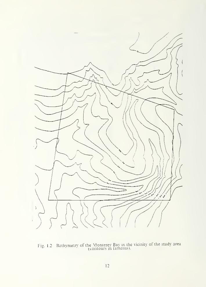
Fig 1 2 Bathvmetrv of the Monterey Bav in the vicinity of the study areato

"' (contours in fathoms).

12

II. THEORY

Water column stability is an expression of the likelihood for the occurance of

vertical motion of water parcels within the water column. It is a function of the

density variation with depth (static stability) and the vertical variation in velocity

(shear). Together, the magnitude of these two components provide an indication of the

dynamic stability of the water column. Irreversible vertical motion (mixing) of water

parcels can occur when there is an imbalance between the horizontal velocity shear and

the thermohaline stratification. The result of mixing is to reduce the vertical variation

of density thereby making the density of the water column more homogeneous. This

results in an increase in the center of gravity of the water column and a consequent

increase in the potential energy of the system. The increase in potential energy is

derived from the kinetic energy of the vertical motion of the parcels which in turn is

derived from the kinetic enersv of the force causing the imbalance in the densitv or

velocity profiles (Pond and Pickard, 1983, p. 60). Definition of the parameters that

define stability as applied to this study are discussed below.

A. STATIC STABILITY

Static stability is strictly a function of the vertical variation in the density field

and as indicated by the word 'static' implies no initial motion in the system. Stability

is indicated by the variation in density with depth. A stable density profile is one in

which density increases with depth. Consequently gravitational forces will not impart

any motion to the water parcels. However, if the density profile decreases with depth

then heavier water overlies lighter water and the result is for the lighter water to rise

while the heavier water sinks (vertical motion) in order to reestablish a gravitational

balance.

Density in the ocean is a function of temperature, salinity, and pressure in order

of decreasing importance. However a more useful parameter is sigma-t which is

defined as:

(Tt

= (p(t,s,0) - 1000) kg/m 3 (eqn 2.1)

13

This parameter is useful in that it allows for a better estimate of what the density

difference between two water parcels would be if they were at the same level. Sigma-t

values were calculated from the temperature and salinity profiles obtained from the

CTD data. The quantitative evaluation of water column static stability is given by the

stability parameter "E" which is expressed as follows:

E = 1 p 6crt

6z (eqn 2.2)

The 6<rt5z term represents the vertical gradient of density.

The buoyancy frequency defines the natural or resonant frequency that a parcel

would oscillate at if displaced vertically from its stable position within a statically

stable fluid. It is quantified as the square root of the product of the static stability

parameter "E" and the gravitational constant "g" and is symbolized by "N".

N 2 = g \ E (eqn 2.3)

The buoyancy frequency is also the maximum frequency of internal waves in water of

stability "E" (Pond and Pickard, 1983. p.30).

B. DYNAMIC STABILITY

Dynamic stability is an indicator of the effect that the vertical variation in

velocity (shear) will have on the generation of vertical motion/turbulence within a

water column of stability "E". Therefore it is a function of both the static stability and

the magnitude of the shear. A quantitative expression for dynamic stability is the

"gradient ' Richardson number which is the ratio of the square of the buoyancy

frequency to the square of the velocity shear:

Ri = (N 2) / (6u. 6z)

2 (eqn 2.4)

A critical value of 0.25 has been established from turbulence theory as the cutoff

between dynamic stability and instability (Pond and Pickard, 1983. p. 60). Values of Ri

> 1,4 indicate that the vertical gradient of velocity is insufficient to generate sustained

turbulence and therefore dynamic stability is is sustained. The converse is true for

values below the critical value. This ratio mav also be viewed as the ratio of the

14

potential energy of the column expressed by the density field and the kinetic energy

expressed by the velocity field.

C. DOUBLE DIFFUSION

Instability in an otherwise statically stable environment may also occur from

double diffusion which is the result of the difference in the molecular diffusivities of

temperature and salt within a fluid causing an imbalance in the density field. The

diffusivity of temperature is approximately 100 times greater than that of salt; thus

double diffusion may occur when two masses of approximately the same density, but

different temperature and salinity are in contact within a statically stable environment.

The difference in the speed of molecular diffusion for temperature and salt results in a

relatively rapid exchange of heat without a compensating exchange of salinity thereby

resulting in a change in the densities of the two water masses. There are three possible

combinations of temperature and salt between the two water masses which result in

three entirely different conditions: ie. double diffusive instability, layering, and no

motion.

1. Case I: Double Diffusive Instability

Double diffusive instability may occur if there is warmer, saltier water over

cooler, fresher water (negative temperature and salinity gradients). The upper layer

cools while the lower layer warms however, the salinity exchange is not rapid enough

to compensate for the increasing density of the upper layer and the decreasing density

of the lower layer. Thus, a negative density gradient is formed, and the boundary

between the two layers becomes unstable. Consequently, the lower layer tries to rise

while the upper layer tries to sink thereby resulting in mixing. Experiments have

shown this mixing to occur as thin columns/filaments of each layer infiltrating the

adjacent layer, this type of mixing is described as "salt fingering" (Pond and Pickard,

1983, p.31)

2. Case II: Layering

An intensification of the stable density gradient between layers occurs when

cooler, fresher water is over warmer, saltier water (positive temperature and salinity

gradients). As the upper layer warms the density decreases while the converse is

happening in the lower layer. Again the salinity exchange is not rapid enough to

compensate for the density changes. When the temperature difference is large the

warming of the upper layer by the lower layer will cause it to rise due to its reduced

15

density . The lower layer will attempt to sink due to cooling and increased density.

This will lead to a breakdown in the interface between the layers thereby resulting in

mixing.

3. Case III: No Motion

In the case of warmer, fresher water over cooler, saltier water (negative

temperature gradient, positive salinity gradient) the density difference is reduced as the

upper layer cannot get denser than the layer beneath it. Therefore no motion occurs.

In order for double diffusion to result in instability, the gradients of temperature and

salt must be the same (Pond and Pickard. 1983,p.32).

16

III. DATA ACQUISITION AND PROCESSING

A. DATA ACQUISITION

Temperature, conductivity, and velocity data analyzed in this study were acquired

from 3 to 5 October, 1984 by the U.S.S. DOLPHIN and R/V ACANIA, which

sampled a square-shaped region centered at 36° 44.5'N, 122° 03.0'W, approximately 22

km west of Moss Landing, California (Fig. 1.1). The R/V ACANIA made seven

circuits of the edge of the region while U.S.S. DOLPHIN sampled the interior of the

region. The vessels were equiped as follows.

1. U.S.S. DOLPHIN Instrumentation

The U.S.S. DOLPHIN was fitted with a 5m high tripod structure near the

bow of the submarine. This structure was used to support the temperature,

conductivity, and depth sensors. The CTD sensors consisted of Seabird Electronics

thermistor and conductivity cell, and a Viatran model 304 strain gauge pressure sensor.

The data from these sensors were digitized and stored on 9-track magnetic tape.

Velocity profiles relative to the submarine were measured by T.P. Stanton with

an R-D Instruments acoustic doppler profiler mounted at deck level, 2m forward of the

base of the instrument tripod. The acoustic profiler had an upward-looking, 4-beam

Janus configuration. The beam angles were rotated 45° in azimuth from the forward

and cross axes of the submarine in order to minimize acoustic reflection from the

instrument tripod. Despite this rotation, reflections from the tripod were received by

the aft transducer sidelobes causing the second and third velocity bins to have

unreliable data. The acoustic beams were inclined 30° from the vertical axis. Acoustic

pulses were transmitted at 1.2 MHz from all four beams at a repetition rate of 5

pings sec. The received signal was range-gated into 30 sections corresponding to lm

length vertical bins, providing profiles of doppler velocities in the 30m above the hull of

the submarine. The radial doppler shifts were resolved into orthogonal velocity

components by differencing the doppler shifts of each bin in opposing beams using the

relationship:

V13

= ((f, - f3)/4f ) x C sin(9) (eqn3.1)

17

V24

= ((f2

- f4) 4f ) x C sin(G) (eqn 3.2)

V..: velocity component resolved from the "i"th and "j"th beams

fQ

: transmitted frequency

f : received doppler shifted frequency from the "i"th beam

CQ

: velocity of sound at the transducer face

6: beam inclination from the vertical

These two orthogonal velocity measurements were then rotated by 45° to give the

forward and cross velocities. Velocity components were averaged for 10 seconds to

reduce the high noise level inherent in pulsed incoherent acoustic doppler systems

which principally arises from trying to resolve small doppler frequency shifts within

short range intervals. The platform referenced velocity components were recorded and

displayed on a Hewlett-Packard 216 computer.

Other instrumentation onboard R/V DOLPHIN, though not used in this

study, included microstructure measuring equipment used by T.R. Osborn and R.G.

Lueck. These consisted of 3 fast response thermistors, 2 airfoil shear probes and 3-axes

accelerator. The airfoil probes were used to measure the time derivative of orthogonal

components of horizontal velocity (du dt, dv/dt). The time derivative is then converted

into a measurement o[ shear. The scales of the shear measured by this method is on

the order of 0.01m to 0.5m. Use of these instruments is described in detail by Osborn

and Lueck (1985). The fast response thermistors were used to measure fine-structure

temperature gradients. The analysis of these measurements of mixing activity is being

performed by T.R. Osborn and E.C. Itsweire.

Additionally, there were two acoustic transducers which transmitted an 80

KHz pulse in the forward and vertical directions with the intent of measuring the

scattering cross-section of the backscatterers in the volume ahead and above the

submarine. These were used by D. Farmer and C. Crawford to investigate the nature

of acoustic back and side scatter at this frequency.

2. R/V ACANIA Instrumentation

R/V ACANIA utilized several types of instruments to measure the

temperature and conductivity of the upper ocean between the surface and in excess of

115m depth. Ocean skin temperature was measured with a Rosemont platinum

resistance thermometer (5.0 mdeg absolute calibration) suspended from a boom over

the side of the ship such that the thermometer remained within the upper few

18

centimeters of the surface. Near surface (2m) temperatures and conductivities were

measured with a pump-through Seabird thermistor and conductivity cell located in the

ship's seachest. Continuous measurement of temperature and conductivity between 5

and 115 meters was made by towyoing a Neil Brown Instrument Systems Mk Ill CTD.

The CTD consisted of a combination thermistor and platinum resistance thermometer

(0.5 mdeg resolution, 5.0 mdeg absolute calibration), platinum electrode conductivity

cell (0.001 mmho resolution, 0.01 nominal accuracy), and an electrical strain gauge

pressure sensor (10 cm resolution). During the towyo the CTD package was raised and

lowered between specified depth limits while maintaining a constant ship speed of

approximately 5 knots. By this method a continuous series of near vertical

temperature and conductivity profiles were obtained. A spatial resolution for the

vertical section was achieved on the order of 0.5km by 0.5m based on the distance

covered in the time to complete an upcast/downcast and the binning of temperature

and conductivity every 0.5m of depth. This sampling resolution was used to determine

the T, S, (7t

. and N structure of the upper 100m of the water column on a scale

comparable with the shipboard ADVP measurements. Thus a valid comparison

around the perimeter of the study area could be made between the static stability as

determined from the CTD data and the shear stability determined from the ADVP

data. Location (latitude/ longitude) information for each CTD profile was obtained

from an Internav LC408 LORAN C receiver (25m resolution, 100m accuracy).

Velocity profile measurements below the ship were made with an Ametek-

Straza acoustic doppler profiler model DCP4015 (ADVP). This profiler has a 4-beam

Janus configuration transducer aligned with the forward and cross axes of the ship

(Fig. 3.1). Acoustic pulses were transmitted at 300KHz even-

0.6 seconds (1.67

pings/sec) with a 5 msec pulse duration. The received signal was range-gated into 32

bins giving a 3m vertical bin size; the shallowest range bin was centered at 7.5m depth.

The forward and cross velocity components for each depth level were computed by

differencing doppler shifts from complementary beams as in the U.S.S. DOLPHIN

(section A.). Forward and cross velocity estimates from each ping were rotated into a

North-South coordinate system using heading information from the ship's Mk9 Sperry

gyro. The resolved velocity components were then averaged over 2 minutes in order to

reduce the doppler frequency noise level as well as noise due to the pitch and roll of

the platform. As indicated by Kosro (1985). when using comparable averaging

intervals and moderate sea conditions, pitch and roll affects the vertical velocity

19

component the most with velocity overestimates on the order of 3 - 4 cm sec.

However, the horizontal velocity components are affected on the order of less than 1

cm, sec; thus the horizontal velocity estimates may be calculated with minimal error

when pitch and roll corrections are ignored, particularly for the low sea states

encountered during these measurements.

The ADVP measures velocity profiles relative to the vessel. Absolute current

profiles may be derived by measuring and removing the ground referenced ship's

velocity. In this study only the shear profiles will be used as high resolution profiles

were needed for the construction of Richardson Number profiles and the ship's velocity

cannot be determined to comparable accuracy with only two minutes averages;

typically 15 minutes are needed to resolve the ship's velocity to 10 cm sec using

LORAN C.

B. DATA PROCESSING

The stability of the water column and the processes affecting it were examined by

analyzing the temperature, salinity, sigma-t, and velocity fields. Stability is a function

of the vertical gradients of density and velocity, but since the water mass structure is

not readily apparent in the density field alone, the temperature and salinity fields were

also analyzed. Analysis was accomplished by the construction of graphical displays of

contoured vertical sections, profile plots, and horizontal vector plots. The temperature,

salinity, sigma-t. and static stability fields were constructed from the R/V ACANTA

CTD data, which provided information from 5.0m to 115.0m depths. These fields are

displayed as both contoured vertical sections and profile plots. L'.S.S. DOLPHIN

CTD data was not used in the construction of these fields as information was limited

to the cruise depth of the submarine and thus had limited vertical range. Velocity

fields were constructed from both the R/V ACANTA and U.S.S. DOLPHIN ADVP

data sets and were displayed as profile plots and horizontal vector plots. Richardson

number fields were constructed by combining the sigma-t and velocity fields from the

R/V ACANTA CTD and ADVP data sets and are displayed as profile plots.

Contoured vertical sections were chosen for the temperature, salinity, and sigma-t

fields because they provided a ready depiction of the spatial variability of a parameter

within a particular section as well as an indication of the temporal variability through

successive vertical sections. The vertical sections were constructed from 2.0m vertical

averages of the R V ACANTA CTD data. Vertical averaging was necessary in order to

20

reduce the noise level in the contouring procedure. Individual vertical sections may be

considered to be approximate "snapshots" of the variability expressed in the

temperature, salinity, and sigma-t fields as they represent data collected within

approximately one hour along a Skm horizontal section.

Averaged and staggered profile plots were constructed for the parameters of

temperature, salinity, sigma-t, velocity, static stability, and Richardson number. The

plots are useful in that they provide a more detailed depiction of the vertical variation

of a parameter than does the contoured vertical section. Thus, small scale vertical

variability associated with some processes such as internal waves and double dilTusion

are more readily apparent. Also, in combination with the contoured vertical sections, a

better understanding of the temporal and spatial variability of the fields of interest may

be made. The averaged profiles of temperature, salinity, and sigma-t were constructed

by side-averaging the vertical profiles of these parameters at 2.0m vertical resolution.

The standard deviation about these profiles was also calculated and depicted by dashed

profiles on either side of the averaged profile. Included with the side-averaged profiles

is a composite profile which represents the mean of the side-averaged profiles.

Averaged profiles of static stability were constructed from 3.0m vertical resolution side-

averaged profiles to correspond with the resolution of the ADVP data used in the

calculation of the Richardson number; standard deviation was not calculated. Critical

value limits are expressed on the E and Ri plots by a vertical dotted line. Staggered

profiles were constructed for temperature, salinity, sigma-t, and static stability from the

0.5m resolution CTD data.

Horizontal vector plots of velocity were constructed for the 25m and 75m depth

levels from the R, V ACANTA ADVP data for the second through seventh transits of

the study area. The velocity difference between these two levels (shear) was also

constructed. Together these plots served to provide information on the tidal and large-

scale current flow. The 25m and 75m depth level was chosen because they defined the

upper and lower depth limits of the section of the water column exhibiting the greatest

activity in terms of temperature and salinity variability. This permitted a comparison

between the dynamic (velocity) forcing and the static forcing on stability.

21

cz>

C_3

Fig. 3.1 Illustration of 4-beam Janus configured ADVP.

22

IV. OBSERVATIONS

A. GENERAL DESCRIPTION

A general depiction of the spatial variability present in the analyzed fields of

temperature, salinity and sigma-t are presented in the side-averaged contoured vertical

sections (Figs. 4.1 - 4.3). It is readily apparent that there is considerably more

variability in the temperature and salinity vertical sections than in the density,' sigma-t

vertical section. This is due to a tendency for the variations in temperature and salinity

to compensate each other resulting in a more consistent density field. This is evidenced

particularly by the compensation exhibited in the eastern side panel comparing the

strong thermal gradient between 35m and 45m with the salinity minimum at the same

depth levels. Overall, the density field strongly reflects the temperature field; however,

where there are strong salinity gradients, salinity variations are reflected in the density

field.

Mean profiles of temperature, salinity, and sigma-t for each side and transit of

the study area depict the temporal variability in the vertical variation of these

parameters (Figs. 4.4 - 4.15). Of note are the consistently strong thermal gradients

between 15m and 35m depicted in the profiles for the east and south sides (Figs. 4.5

and 4.6). The north and west sides exhibit considerably more temporal variability in

their temperature profiles (Figs. 4.4 and 4.7). This variability is oscillatory such that

the composite profile (average of all seven circuits of a side) has nearly constant slope.

The salinity profiles (Figs. 4.8-4.11) suggest a migration of parcels of less saline water

between 25m and 65m through the study area. Sigma-t profiles for the east and south

sides (Figs. 4.13 and 4.14) reflect the temperature profiles especially with regard to the

strong thermal gradients as was indicated in the contoured vertical sections. The

sigma-t profiles for the north and west sides (Figs. 4.12 and 4.15) however do not tend

to reflect the vertical variability evident in the temperature profiles, and instead tend to

monotonically increase with depth. This may be attributed to compensation by the

salinity field.

B. STATIC AND DYNAMIC FORCING MECHANISMS

As discussed in Chapter I, there are several forcing mechanisms which can induce

variability in the temperature, salinity, density, and velocity fields and thus ultimately

the stability of the water column. The mechanisms investigated in this study were

upwelling, bottom topography, tidal flow, current systems, and internal gravity waves.

Analysis of the temperature, salinity, sigma-t. and velocity fields in conjunction with

the atmospheric and tidal conditions present during the study indicated that all of these

mechanisms were present with the exception of upwelling. Evidence for these

mechanisms is discussed below.

1. Upwelling

The atmospheric conditions several days prior to and during the study period

were characterized by a high pressure ridge off the central California coast with a weak

pressure gradient over the coastal areas. The resulting low level winds were from the

north-northwest at approximately 5 - 8 knots. This weak NNW flow was modified by

the diurnal land-sea breeze fluctuations. A sea breeze regime commenced in the early

afternoon with a backing and increase in wind speed to WNW at 8 - 14 knots. This

regime persisted until midnight when the winds veered back to NNW and diminished to

2 - 4 knots (weak land breeze regime). The synoptic scale flow resumed in the early

morning just prior to sunrise. The low winds and generally offshore flow resulted in an

absence of the summertime pervasive coastal status and fog . Low winds also provided

for calm sea conditions. Due to the weak NNW flow, coastal upwelling was severly

diminished and thus deemed to be negligible as a forcing mechanism during the study

period.

2. Bottom Topography

The bottom topography of the study area, as mentioned previously, was

dominated by the steep slopes of the Monterey Canyon (Fig. 1.2) The canyon axis

roughly corresponded with the NE-SW diagonal of the study area with slope towards

the southwest, but is deflected somewhat from the NE-SW orientation by the presence

of a large topographic ridge projecting southward into the study area from near the

midpoint of the north side. Evidence of the effects of bathymetry on the analyzed

fields is demonstrated in the contoured vertical sections of temperature (Figs. 4.16 -

4.22). Particularly evident is the mass of colder water between 40m and 95m in the

eastern side. This mass is expressed in the vertical section by an upward bulging of the

11.5 and 12.0°C isotherms in the northern half of the eastern side. The bathymetry of

the eastern side is nearly constant at approximately 400 fathoms (800m) for the

northern three-forths of the side then rises to 100 fathoms (200m) at the southeast

corner. Therefore, this colder mass would be indicative of a trapped pool of colder

24

water. Analysis of the 12°C isotherm in the northern side sections also show evidence

of bathymetric channeling as expressed by an downward bulging in the isotherm. The

location of the bulging corresponds with the axis of the canyon and would seem to

represent the channeling of warmer water along the canyon axis. The combination of

the warmer pool in the eastern portion oi" the northside with the cooler pool in the

northern portion of the eastern side indicates that warmer water is being advected

along the canyon axis while the cooler water is displaced along the sides of the canyon.

Channeling of water flow by the canyon may also affect the velocity field, especially

with regard to the oscillatory tidal flow.

3. Tidal Flow

Tidal flow along the California Coast is characterized by two high and two

low tides even' 25 hours, occurring about 50 minutes later every day. The heights of

the two high tides and the heights of the two low tides are not equal in magnitude or in

time between them. During the study period the higher high tide occurred in the early

evening at about 1900 while the lower low tide occurred shortly after midnight. Actual

tide times at Moss Landing were high tide at 1818, 3 Oct and 0839 and 1924, 4 Oct:

low tide occurred at 0140 and 1403. 4 Oct and 0240. 5 Oct.

Tidal effects are most noticeable on the temperature and velocity fields. This

is demonstrated in the contoured vertical sections of temperature (Figs. 4.16 - 4.22) and

the horizontal vector plots of velocity (Figs. 4.23 - 4.27). With regard to the

temperature field, tidal effects are especially evident in the vertical sections for the

northern side expressed by the variability in the 12° and 14°C isotherms. This may be

due to the near parallel orientation of the section with the predominantly east-west

fluctuations in the near surface tidal flow. In circuit 1 (Fig. 4.16) the 12° isotherm is

nearly flat across the northern section at a depth of approximately 60m during a time

corresponding to a period of slack water at high tide. By circuit 2 (Fig. 4.17), the 12°

isotherm slopes upward to the east and a patch of warmer water is evident in the

eastern portion of the section between 60 and 80m; this is during a period o[ ebb flow.

In circuit 3 (Fig. 4.18), a period of flood flow, the 12° isotherm is deeper and slopes in

the opposite direction to the previous circuit, but exhibits a bulge in the isotherm to

representing an intrusion of warmer water. At low tide (Fig. 4.20) the 12° isotherm is

again nearly flat as in circuit 1, however the depth is nearly 15m deeper indicating the

ebb flow introduced warmer water into the study area which depressed the 12D

isotherm. The tilt of the 14° isotherm also reflects the tidal flow. During periods of

25

ebb flow (Fig. 4.17 and 4.22), the isotherm slopes downward to the east whereas the

slope is reversed for flood flow (Fig. 4.18 and 4.21). The 14° isotherm is approximately

horizontal during periods of slack water (Fig. 4.16 and 4.20). Tidal flow may also

distort the temperature and salinity fields through the advection of water parcels such

that the advected parcels have different temperature and salinity characteristics than

the host water. Evidence of tidal induced advection was discussed above with regard to

the influence of bottom topography.

The horizontal velocity plots (Figs. 4.23 - 4.27) exhibit fluctuations in

direction and magnitude corresponding to the tidal period. This is particularly

evidenced by the eastern and western sides. The western side shows a consistent

westerly flow , however the magnitude varies in direct relationship to the east-west flow

reversals observed on the eastern side. The period between the flow reversals is on the

order of 13 hours which corresponds well with the tidal period. The northern and

southern sides, on the other hand, exhibit consistent southerly flow through the study

period: this could therefore be indicative of a general southerly flow (California

Current) with a tidally induced fluctuating east-west velocity component. Bottom

topography induced channeling results in the flow fluctuations being greater along the

eastern side.

4. Currents

Current systems of interest to this study included the California and Davidson

Currents. The Davidson Current is usually dominant during periods of reduced

upwelling as occurred during this study. However, the horizontal vector velocity plots

(Figs. 4.23 - 4.27) along the northern and southern sides of the study area do not give

any indication of the presence of the northward flowing Davidson Current within the

study area, but rather depict a consistent southward flow characteristic of the

California Current. As mentioned above the flow along the eastern and western sides

appears to be modified by tidal flow. Additionally, the current velocities are greater at

25m than at 75m resulting in a negative velocity gradient and providing for shear as a

dynamical forcing on stability. Average velocity differences between the 25m and 75m

depth levels was on the order of 5 cm; sec.

Currents also affect the temperature and salinity fields through advection of

water parcels. This appears evident in the contoured vertical sections of salinity (Figs.

4.2S - 4.34) where a lens shaped minimum in salinity is described by the 33.3 ppt

isohaline at between 25m and 55m depth. Advection of this less-saline lens by the

26

large-scale current flow may be observed in the vertical sections for the north and east

sides where the lens, which initially spans the northside at approximately 45m, is

observed in successive sections to reduce in size and migrate to the east and south.

This southward migration is also evident in the vertical sections for the south and

westsides where smaller parcels of less-saline water are observed to migrate across the

side during the course of the study. An estimate of the speed of migration is

approximately 0.5 km/hr (14cm;s). This is only a crude estimate considering the other

processes which may distort the parcels. The overall southward migration apparent in

these vertical sections is consistent with the general southerly flow observed in the

velocity plots and may be attributed to the California Current system.

5. Internal Gravity Waves

Internal gravity waves affect the temperature, salinity, and density fields

through the intensification and weakening of gradients caused by wave induced

displacements of the density interface. The movement of the internal wave intensifies

temperature, salinity, and density gradients in the direction of movement as the density

interfaces oscillates vertically. A concurrent weakening of gradients occurs behind the

movement of the density interface. The frequency of internal waves is bounded at the

upper end by the buoyancy frequency. A mean buoyancy frequency of approximately

0.6 cph was calculated for the study area though this represents a low value for the

upper bound of the buoyancy frequency as individual profiles values were higher. This

frequency corresponds to a period of 1.7 hours indicating that the shorter period

internal waves should be adequately represented by these diagrams. The lower bound

on the frequency for internal waves is the inertial frequency. The inertial frequency for

the latitude of the study area (36.75°N) was calculated to be 0.0498 cph. The

corresponding inertial is 20.06 hours.

While wave-like features appear evident in the contoured vertical sections,

they are especially evident in the staggered profile plots. This is particularly noticeable

in the staggered profile plots for the eastern and western sides (Figs. 4.35 - 4.37). In

the staggered temperature profiles for the eastside, the area of strongest thermal

gradient (between 15m and 35m depth) is observed to oscillate in a wave-like pattern

with a wavelength of approximately 7km. A second wave pattern is evident between

65m and 85m and is in phase with the upper wave pattern. Similar wave patterns are

exhibited in the staggered profiles of salinity and sigma-t. The western side staggered

temperature profiles exhibit two sets of waves at between 10m and 30m for the upper

27

wave and between 75m and 95m for the lower wave pattern. These two wave patterns

are ISO out of phase which results in a stronger alternating intensification and

weakening of density gradients between them. As in the staggered profiles for the

eastern side, the western side salinity and sigma-t profiles exhibit similar wave patterns

to that displayed in the temperature profiles. This similarity in wave patterns between

all three parameters is due to the movement of internal gravity waves along density

interfaces resulting in an oscillatory or wave motion expressed in the density profiles.

Since the density is not changed by the motion of the internal wave, the temperature

and salinity profiles should exhibit similar wave patterns.

C. STATIC AND DYNAMIC STABILITY

The variability expressed in the displays of temperature and salinity were for the

most part compensating such that the displays of sigma-t exhibited a more uniform

field. This is exemplified in the contoured vertical section of sigma-t (Figs. 4.38 - 4.44).

Consequently, the static stability field could be expected to be stable overall as

exhibited by displays of the static stability parameter (E) and the dynamic stability

parameter (Ri) or Richardson number. Comparison of the averaged profiles of the

static stability parameter (E) (Figs 4.45 - 4.48) and the Richardson number (Ri) (Figs.

4.49 - 4.52) provide an indication o^ the relative importance between the vertical

density gradient and the velocity gradient on the stability of the water column. The E

and Ri average profiles are calculated from 3m vertically averaged density differences

to coincide with the 3m vertical resolution of the velocity data. Consequently, because

gradients of density and shear can occur on scales smaller than this 3m differencing

interval, the Ri profile values represent an upper bound. Many of the maximums in

the Ri profiles correspond with the maximums in the E profiles indicating that the

strength of the density gradient is driving the dynamic stability. Maximums in the Ri

profiles which do not correspond to maximums in the E profiles indicate that there is a

relative minimum in the vertical gradient of velocity (shear) in that portion of the water

column as well as a weak, density gradient. Minimums in the Ri profiles indicate that

the relative magnitude of the shear is greater than the density gradient. Values of Ri

below the critical value indicate that the shear is greater than twice the density

gradient. Of note are the below critical Ri values observed near the top of most

profiles. This is a manifestation of the acoustic profiler caused by sidelobe interference

in the upper bins of the shipboard ADVP.

28

The averaged profiles of the static stability parameter indicate stability through

the vertical extent of the water column. However, the staggered profiles oi' E indicate

thin patches ( < 2.0m thick.) of static instability. This is exemplified in the staggered

profiles for the east (Fig. 4.53) and west sides (Fig. 4.54). As was noted in the

discussion of internal waves, wave like patterns are also exhibited in the staggered E

profiles. The thin unstable patches are indicative of double diffusive processes acting

upon the disturbances in the density field caused by the static and dynamic forcing

mechanisms of bottom topography, tidal and current flow, and internal waves.

Preferred locations of instability and double diffusive processes are in regions of strong,

but opposing temperature and salinity gradients. However, despite the extreme

variability observed in the temperature and salinity fields, the density fields were for the

most part consistent with monotonically increasing gradients, and consequently the

water column is predominantly stable.

29

^ * « cic £ OT a

9 — E "

* - 8|15 57)

~ •s :

r- ub... a< i

<

(fV) tndaa(/v) mdsa

(/Y) tTldsaOvi indsa

Fig. 4.1 Vertical section of side-averaged temperature.

30

(/v) mdaa(M) mdsa

(/y) indsq (ft) iocisa

Fig. 4.2 Vertical section of side-averaged salinity.

31

IT;

(M i^dsQ

5

2<<>

(m indaa

-a. W

(w mdaa(/V) VldaQ

Fig. 4.3 Vertical section of side-averaged sigma-t.

Uj

-̂~,

to <os.*sk CD

^ (_

o J^ (Cs-*' un 0)

£u,

cu

CD

O <—>> o5 en

n oF-

"—

< p

2 Cm

< CU «<J o^ -5

cc

"" —ocuto

G

ooCO

pa *-

— H

c\2

—

'

ovCO

C

to

oa

N o

2 ^CJCD

to

a

CO

—ooCO

C

EE-"

-i ^CJ

CDto

CP3

— ran ^incor^majo^

(/V) mriaa (/f) qidaa

Fig. 4.4 Averaged profiles of temperature (northside).

Co «

U c

oo

c_

>>

£

(-1

o (/j

—<

—o

^<U ^«

< <3

(Ar

) MI^CI (7n m^oa

Fig. 4.5 Averaged profiles of temperature (eastside)

34

Uq

£ Co

=q"—

'

t-. QJ

^ Uo JCo (0^—^ un oi— Uu £-— a;

o r™O <~>> O£ V)

o a;

F- 1^5_<: o

2 0.

< cCJ< 0)

*-» -a

oCDen

a

CO

uoCO

CR3

r M"^ —

ooto

Ccc

aft

03

Oa.

N O- u

2*"

CJoTi

C(8

- t-

2 °ooto

C

~£

2^— —>

CJ

cuto

Ca

2ft

(/v) q^daa (;V) Mldoa

Fig. 4.6 Averaged profiles of temperature (southside).

35

fa

to

QE-uT3oo

o

2<<

Cj

c

oua.

u0)en

C

- E-

u0)

en

-Juoen

Oa

"~8

* °oO

C(0

(/v) rndsa (;f) mdaa

Fig. 4.7 Averaged profiles of temperature (westside).

36

to

2<<

8:

Q C

b «

o o>> V)

o F"E- c

0-

o o>n Cj

n C

inLj

E-

n

CO

a Om o(-> wn C

aL,

c-

P)n

o om or> !fl

n Ca

« —

i

n om CJ

r^ OT

n CMU

in H

o OIT, ai

1—

,

kr) c

aU

r fE-

n CD

o <->

« C

m-^oa

C-E-

iD U") lO tO

(flO Mldaa C/v) m^a

Fig. 4.8 Averaged profiles of salinity (northside).

37

tr. >\ s—

'

1 S

c< r

>

a o

ro

c o

wO iJ

ny:

CQ

in £nn

" -,

Q Oin O

ca

in C_M w

nn

c; o —

(/V) Ml'^CI

c-. c —

(A) MT'-'fl

Fig. 4.9 Averaged profiles of salinity (eastside).

CO

£ois.

QU

uO

oE-

o1/3

< a.-

< -«

«

nn

-f—

i

O um on oo

r> ti

re

uin

r-

nn

a Om on 73

n cfi

uin

r-

n" c\?

o oin 0)

« 2«u

"O f-i

o 73

<n utn a.n C

>—

i

<"> u

m 0)

CO

uCD03

C

U

a oin un mn C

re

uEH

(/v) xndaa (/v) qidoci

Fig. 4.10 Averaged profiles of salinity (southside).

39

to

QE-U-3ao>>

oE-

•z.

<<>

En

9,

"c

en

1 in in in in >n IT- CM n ^- if) <c f~

n in

m CJ

n an

6

CJ

nn

r> UIT CI

rr Xn C

f3

UE-

r>n

CO

c uo cr> y.

n r*

(fl

UE-

ma CJin on 71

ro cidu

inE-

nn

(/V) q-}daa (/V) q^daa

Fig. 4. 1 1 Averaged profiles of salinity (westside).

40

Ito£o

Qb

o

oE-

2

E-I

<

O7)

-a.

< c(0

CO

oCO

cre

—ooen

O0)COr*

reu,

E-

u ^

cum _-n 'EnN O

a.« ENu

ca

. <n "

o

to

re

uE-

(/V) Mldaa (;v) tndoa

Fig. 4.12 Averaged profiles of sigma-t (northside).

41

[0t~-<

tol_

1

<N—

'

-«*.

a ou (/J

—"0 nQ)

o o

£ •—

o u

< r

<>

— pj r>

:i\') Mi<i->a

(0rj

—if)

l

~ —n L>

i.

(«

f3-

to

fw

in

•J~,

r-m

CV

N osrj•—

lO

gr-1

L-!

s

u

(/v) i n<J^u

o

—

a

—uIT,

f3

U

Fig. 4.13 Averaged profiles of sigma-t (eastside).

42

o

Qf-UT3CJ

O

o

2<<!

00

c

0.

in*'

—o0)CO

E-

W

~8

in

en

cs «

m

OasoCJ

u0)03

c

-E-

<oN

CO

CO

(flO Mldaa (/f) mdaa

Fig. 4.14 Averaged profiles of sigma-t (southside).

43

Mj

OKto t-

1*4 I

S*. <-2

Q oE—

CJ(A)

—T3a>

o

£ <_

n oE-

C-

< cZ<

<o

u --.

<>

m

•n

in £

tn

CJ

OOCO

CSO

uE-

- ©

U<n

Ca6

CJ cCJ

CJ

oen^-

EE—

CO—CJ

oCO

Cto

uE-

N

to

>gE-

tS

iTv id in in un \fl %no ;c r* a> a c -<

(/vO mdo<3 (/V) xndaa

Fig. 4.15 Averaged profiles of sigma-t (westside).

44

m « » *>

(/V) qidsa (/V) Uldaa

Fig. 4.16 Vertical section of temperature for circuit 1.

45

(m tndaa(/V) mdaa

n n *> r> <r> « o « o r) »-

(fV) t^daa (/V) t^daa


46

a r* x 3

(/V> Uldaa (A') lHd3Q

(/V) mdaa(/v) iridsa


47

(/V) ipdaa (m Lndaa

< t< >

>

' ' s*)*?*> rtr>tf>r>nr!*">*i

5o

S= S

< J 72n5* I

(/v) indaa (zv) todsa


48

— ry 71 * <ft 10

(W) l^dSQ (ff) q^daa

— wo(tt) \ndaa (fV) qidaa


49

to

5to ~

/) =

O to Q>>z M

* w.3

71< =— .« a

<• —

'

«< ^

(AO mdaa (/V) Mldaa

(/V) qidaa (/v) tnciaa


50

C/) -

O -r -

^>o ffl

Vr" ^U a^ m& -;

c

>ini _

% = -

.V)< N— S n

(/v) ^daa W q^dsa

(/V) U^daa (A') tTldaa


51

V ^ // / r / l A\

// /

/

5 cm/s

w

1 I V

I \ \

/

/

i

ft

\o \, V I i

Fig. 4.23 Horizontal velocity difference plots for 75-25m levels (circuit 2).

52

5 cm/s

\

/

^/X\

\V\

a.

\*J ^

\ \ \

\ yi /

Fig. 4.24 Horizontal velocity difTerence plots for 75-25m levels (circuit 3}

53

5 c m/s

s \ \

\

'I

r\

v\ \

v

\ N\\\\\\\\\ <\ \S \ \ \ \

p __£, \o No" >D No \3 \j '« ^ ^ ^ ^ "° D C^X.^/


54

V

/sA/

P a-f

/

5 cm/s

/ P

1//•

\


55

/ iV V/ \, i

V

-o

5 cm/:

//VlvOCC^XVvw> V

\ x\\


56

(H) tndaa (/V) Mldaa

t/v) indaa (/f) tndaa

Fig. 4.28 Vertical section of salinity for circuit 1.

57

(W) LRdaa(/v) tndsa

(f\) mdaa(fV) mdsa


58

(Ft) mdaa(ff) indaa

im indaa(/v) uidsa


59

(N) ^daa ifi) M^d

(fY) Uldaa (/V) Uldaa

Fig. 4.31 Vertical section ofsalinitv for circuit 4.

60

CO £-r a.

5 I 3

2-3<

>

(/V) meted (/V) UldsQ

(/Y) i^daa(/V) md»a


61

W) tndaa UY) tOdsa

ifY) i^daa (w) tndsa


62

Co

> C" a

O »*&§£

g=> I

lcz

E- c ".. c _< rj *— a iz

<

<

«8

(w) qiciaa</v) mdsa

(/V) Uldaa (/V) qidaa

Fig. 4.34 Vertical section of salinitv for circuit 7.

63

R/V ACANIA: Towyoed CTD (EASTSIDE)

2327. 3 OCT - 0022, 4 OCT 1904

10.0 12.0 14.0 18.0 18.0 20 22.0 24.0 26.0 28.0 30.0 32.0 34.0 36.0 38.0 40.0

Staggered Temperature (DEG C)

R/V ACANIA: Towvoed CTD [WESTS IDE)

2105 - 2211. 3 OCT 1984

10.0 12.0 14.0 18.0 18.0 20.0 22 24 26.0 28 30. 32.0 34.0 36 38 40

Staggered Temperature (DEG C)

Fig. 4.35 Staggered profiles of temperature.

64

Q.4)

D


2327, 3 OCT - 0022. 4 OCT 1984

33.0 34.0 35.0 36.0 37.0

Staggered Salinity (PPT)38.0 39 40.0

a01

Q

33.0

R/V ACANIA: Towyoed CTD (WESTSIDE)

2105 - 2211, 3 OCT 1984

34.0 35.0 36.0 37 30.0

Staggered Salinity (PPT)40

Fig. 4.36 Staggered profiles of salinity.

65

5.0


2327, 3 OCT - 0022, 4 OCT 1984

3,

0)

Q

24.

5

25.5 26.

5

27.5 28.5 29.5

Staggered SIGMA-T30.5 31.5

5,

aQ

R/V ACANIA: Towyoed CTD (WESTSIDE)

2105 - 2211, 3 OCT 1984

24.5 25.5 26.5 27.5 28 5 29.5

Staggered SIGMA-T30.5 31.5

Fig. 4.37 Staggered profiles of sigma-t.

66

(m ^daa(fY) qidaa

i/v) indaa (/v) tndaa

Fig. 4.38 Vertical section of sigma-t for circuit 1.

67

(fV) mdag (m u^daa

r> *> fi r.

(w) iridaa (fV) ^daa

Fig. 4.39 Vertical section ofsigma-t for circuit 2.

68

(m tr.dsa (W) qidsa

(m mdaa (/V) indaq


69

6»

_ -~ /

w 5 c

ZZ §

>>o a

1:1

2/ o S 8-

1/ *

'. \V

(/v) mdaa (/v) vndaa

l/Y) Uldaa(/V) Uldaa


70

>

(W) q^daa (yf) tndaa

(/y) indaa(/V) tndaa


71

(/v) tndaa(W) t^daa

(M) ip,d3Q (/V) mdaa


72

(fY) qidaa(W) ^idaq

hiQ

^3

> Z

u<

<

(/V) mdaa (/V) Uldaa


73

to

OSo

ou

o

00

o

3

q O

_. to

Ca

o o

oo a>

C

(/V) mdaQ

q o

en

Oa

ou

o O

-_; <n

£a

o o

o O

oO 4)- "cat

(/V) MldOQ

Fig. 4.45 Average profiles of the static stability parameter (E)

for the northside.

74

ob

ICO

§

OuOh

—W

(0

CO

T30>em

E

(/V)t«daa

ob

Oo.cou

o O

o tt>

• on

C

o O

CD

— >C<a

oH

ca

H

(/v) tndsa

Fie. 4.46 Average profiles of the static stability parameter (E)tor the eastside.

75

O

>>

JS

cCXI

<cua>

3

(/V) tpdaa

Fig. 4.47 Average profiles of the static stabilitv parameter (E)for the southside.

76

Ito

Ir>a.

o

a.

—

_o

a—xn

o.

e

oO tl

— to

o O

tn

oO <D

c

q O

oo <u

,CCO

(/V) ^daa

oa£ou

Ces

a o

CatU

o<uen

C(9UH

(/y) t^daa

Fig. 4.48 Average profiles of the static stability parameter (E)for the westside.

77

5a;o

3Zaotn

T5

(0

to

U0>

3

(/r) qrisQ

1'

i i

Fig. 4.49 Average profiles of the Richardson number (northside).

78

B

S

o

zcor>

a>-

c

ex

0>

3

C/r) »o«*»a

— M O •* a « I*

Fig. 4.50 Average profiles of the Richardson number (eastside).

79

ou

u

J2

3Zco

ce

(0

a>

o— e.

EoO

(/T) mdaa

{JTi mdsQ

Fig. 4.51 Average profiles of the Richardson number (southside).

80

to

65

o

£ua.'

EC

"it

ci~a-

W m«i»a

W cpd»a

Fig. 4.52 Average profiles of the Richardson number (westside).

SI

SoK "*

CO(71^

ki K1.3Q o—

CJ*

-oft?

r\?u> no n>>

3J1

o kt-

o< mz r»< ft?

C) C*3

< ft?

(/f) q;d3Q

Fig. 4.53 Staggered profiles of the static stability parameter (eastside).

82

I^ T*.— ccs—s 0>f~\ ^H

E—

1

[^

:

)

sj

no _7r>> ~m

£

E~" I

< m"^ —2 pj

<CJ<;

>0>

o o o o om m

inin mo —

(/0 mdaCI

Fig. 4.54 Staggered profiles of the static stability parameter (westside).

83

V. SUMMARY AND CONCLUSIONS

Water column stability is determined by the interaction of dynamic and static

forcing. Examination of the stability and the driving mechanisms in the upper 100m of

the measurement area was accomplished by the graphical display of the temperature,

salinity, sigma-t, and velocity fields as well as the static stability parameter and the

Richardson number. The analysis of these displays indicated a rapidly changing

environment and complex horizontal structure.

Several forcing mechanisms and their effect on stability were investigated within

the context of the analysis fields and the atmospheric and tidal conditions existing

during the study period. These mechanisms were upwelling, currents, tides, bottom

topography, and internal waves. All of the mechanisms were found to be a factor in

the stability of the water column with the exception of upwelling. The California

Current was found to dominate with an apparent absence of the Davidson Current.

The analyzed fields of temperature, salinity, density, and velocity exhibited

considerable spatial and temporal variability. This variability took the form of wave-

like patterns, migrating parcels, fluctuating isolines, and intensification/weakening of

gradients. These disturbances could be attributed to the forcing mechanisms of bottom

topography, tidal flow, current systems, and internal gravity waves. The shear, as

measured between 25m and 75m was calculated to be at least 5.0 cm/sec. The presence

of shear provided for the possibility for dynamic instability. Double diffusive processes

were indicated to be a factor in stability by the small reversals in the density field

revealed in the staggered static stability profiles. However, despite the large variability

evident in the temperature and salinity fields, the sigma-t field did not exhibit

comparable variability. This indicates that most of the temperature and salinity

disturbances were density compensating and thus maintained stability.

The stability of the water column was found to be both statically and

dynamically stable on the average as would be expected considering the episodic nature

of instability. However, small patches of instability were identified in the staggered

profiles of static stability which were predominantly located in the 25m to 75m region

of the water column. This region of the water column is also where the greatest

variability in the thermohaline and velocity fields occured. The patches of instability

84

appeared to he primarily due to double diffusive processes initiated by periodic

intrusions of warmer, less saline water.

85

LIST OF REFERENCES

Blumbere. R.E.. Mesoscale spatial and temporal variations of water characteristics in theCalifornia Current region off Monterey Bav in 197J- 1974. M.S. Thesis. NavalPostgraduate School, Monterey, California, "September, 1975.

Breaker, L.C., The space-time scales of variability in oceanic thermal structure off thecentral California coast. Ph.D. Thesis, Naval Postgraduate School, Monterey,California, December, 1983.

Christiansen, C, Microstructure profiles. M.S. Thesis, Naval Postgraduate School,Monterey, California, March, 1"980.

Gargett. A.E., T.R. Osborn and P.W. Nasmvth, 1984: Local isotropv and the decav of" turbulence in a stratified fluid. J. Fluid Mech. 144,231-280.

Garrett. C. and W. Munk, 1972: Space-time scales of internal waves. Geophys. FluidDyn., 2, 225-264.

Greer, R.E., Mesoscale components of the geostrophic flow and its temporal and spatialvariability in the California Current region off Monterey Bav in 19/3-74. M.S.Thesis, Naval Postgraduate School, Monterey." California. September. 1975.

Kunze. E. and T.B. Sanford. 1984: Observations of near-inertial waves in a front. J.

Phys. Oceanogr., 14, 566-581.

Munk. W., Internal waves and small scale processes. Evolution of PhvsicalOceanography, B.A. Warren and C. Wunsch, Eds., The MIT Press, 1981.

Osborn. T.R. and R.G. Lueck, 1985: Turbulence measurements with a submarine. J.

Phys. Oceanogr., 15, 1502-1520.

Pollard. R.T., 1979: Properties of near-surface inertial oscillations. J. Phys. Oceanogr.,10, 385-398.

Pond. S. and G.L. Pickard, Introductory dynamical oceanography. 2d ed.. PereamonPress, 1983.

Turner. J.S., 1973: Buoyancy effects in fluids. Cambridge Univ. Press, London.

Turner, J.S., Small-scale mixing processes. Evolution of Phvsical Oceanographv, B.A.Warren and C. Wunsch, eds. The MIT Press, 1981.

Weller R.A., 1982: The relation of near-inertial motions observed in the mixed laverduring the JASIN (1978) Experiment to the local wind stress and to the quasi-geostrophic flow field. J. Phys. Oceanogr., 12, 1122-1136.

Wickham, J.B^ A.A. Bird, and C.N.K. Mooers. 1986: Mean and variable flow over theCentral California continental margin, 1978 to 1980. Cont. Shelf Res., (in press).

86

INITIAL DISTRIBUTION LIST

No. Copies

1. Defense Technical Information Center 2Cameron StationAlexandria, VA 22304-6145

2. Library, Code 0142 2Naval "Postgraduate SchoolMonterey. CA 93943-5002

3. Chairman. Department of Oceanography 1

Code 68Naval Postgraduate SchoolMonterey. CA 93943-5000

4. Office of the Director 1

Naval Oceanoaraphv Division (OP-952)Department of the NawWashington, D.C. 20350

5. Commander 1

Naval Oceanoeraphv CommandNSTL. MS 39522

6. Commanding Officer 1

Naval Ocearfographic OfficeBav St. LouisNSTL, MS 39522

7. Commanding Officer 1

Naval Ocean Research and Development ActivityBav St. LouisNSTL, MS 39522

8. Chief of Naval Research 1

800 N. Quincv StreetArlington, VA 22217

9. Dr. Edward B. Thornton 3

Code 68Naval Postgraduate SchoolMonterey, CA 93943-5000

10. Dr. Timothv P. Stanton 3

Code 68Naval Postgraduate SchoolMonterey, CA 93943-5000

11. Mrs. Bettv M. Beale 5

P.O. Box 735Lavtonville, CA 95454

87

tt f£<5/i^

'

<b

TITLE NUMBER .CUSTOMER NUMBER

LIBRARY: —Monterey, California 93953

Binding in

Everything

CONTENTS

INDEX

Bind without Index

ISSUE CONTENTS

Discard

Bind in Place

i Gather at Front

i Advertisements

Front Covers

|

Back Covers

11st only

'Accents

Imprints

F B NP

IN OUT

1

EDWARD G. BEALE JR.

imp

Thesis B2858

Special Instructions

Buck Color

Print Color

Trim Height

Ht Inches

Over Thick

For Title

Extra Lines

Extra Coll

Hand Sew

Slit

Rules

1st Slot No

Vol Slot No

Year Slot No

Call # Slot

Imp Slot No

Type Face

Price

Mending

Map Pockets

2 Vols in 1

RosweLLbOOl<l31Nt)INQLIBRARY DIVISION

2614 NORTH 29th AVENUEPHOENIX, ARIZONA 85009PHONE (602) 272-9338

ACTUAL TRIM

SPINE

BOARD DIM

CLOTH DIM

CLOTH BIN

DATE

JOB

LOT

ROUTE

SEQ NO

$6A^

DUDLEY K' RYNA' CHOOLMOM r A 93943-6008

ThesisB2858.1

2092J*

Beale

Analysis of water co-lumn stability usingshipboard and submarinedensity and shear mea-surments.

Thesis

B2858c.l

22C32h

BealeAnalysis of water co-

lumn stability usingshipboard and submarinedensity and shear mea-surments.

analysis of water column stability using shipboard and submarine … · 2018-01-16 · calhoun: the...

Documents