analysis procedures manual chapters 1-4 · exhibit 6-5 level of service criteria for weaving ......
TRANSCRIPT

Analysis Procedures Manual
Version 1
Original Publication Date: April, 2006 Last Update: July, 2018
Oregon Department of Transportation Transportation Development Division
Planning Section Transportation Planning Analysis Unit
Salem, Oregon

Analysis Procedure Manual Version 1 ii Last Updated 07/2018
ACKNOWLEDGEMENTS The following individuals were contributors in the preparation of this manual. Oregon Department of Transportation Kent Belleque, P.E. Alexander Bettinardi, P.E. Rod Cathcart Don Crownover, P.E. Brian Dunn, P.E. Simon Eng, P.E. Christina Fera-Thomas Meghan Hamilton Mark Johnson, P.E. Chi Mai, P.E. Christina McDaniel-Wilson Joseph Meek III, P.E. Nancy Murphy Thanh Nguyen, P.E. Douglas Norval, P.E. Robert Nova Gary Obery, P.E. Peter Schuytema, P.E. Dorothy Upton, P.E. DKS Associates, Inc. John Bosket, P.E. Carl Springer, P.E. Bob Schulte CH2M Hill Craig Grandstrom, P.E. Copyright @ 2006 by the Oregon Department of Transportation. Permission is given to quote and reproduce parts of this document if credit is given to the source. This project was funded in part by the Federal Highway Administration, U.S. Department of Transportation. The contents of this report reflect the views of the Oregon Department of Transportation, Transportation Planning Analysis Unit, which is responsible for the facts and accuracy of the information presented herein. The contents do not necessarily reflect the official views or policies of the Federal Highway Administration.

Analysis Procedure Manual Version 1 iii Last Updated 07/2018
This manual is provided to you by the Oregon Department of Transportation (ODOT) "as is" without warranty of any kind. ODOT makes no warranties, either express or implied, including, but not limited to the implied warranties of merchantability, fitness for a particular purpose, and noninfringement. The entire risk as to the quality and performance of this information is with you. You are advised to test use of the information thoroughly before you rely on it. The author and ODOT disclaim all liability for direct, indirect or consequential damages, arising out of your use of the manual.

Analysis Procedure Manual Version 1 iv Last Updated 07/2018
Table of Contents
1 INTRODUCTION – SEE APM VERSION 2 PREFACE AND CHAPTER 1 ............................ 1-1
2 MANAGING ANALYSIS PROJECTS – SEE APM VERSION 2 CHAPTER 2 ........................ 2-1
3 TRANSPORTATION SYSTEM INVENTORY - SEE APM VERSION 2 CHAPTER 3 .......... 3-1
4 DEVELOPING DESIGN HOUR VOLUMES - SEE APM VERSION 2 CHAPTERS 5 AND 6 ........................................................................................................................................................ 4-1
5 ASSESSING PERFORMANCE ....................................................................................................... 5-1
5.1 PURPOSE – SEE APM VERSION 2 CHAPTER 4 .................................................... 5-1
5.2 CRASH ANALYSIS - SEE APM VERSION 2 CHAPTER 4 ....................................... 5-1
5.3. PEAK HOUR FACTORS – SEE APM VERSION 2 SECTION 5.8.1 EXISTING PEAK HOUR FACTORS AND SECTION 5.8.3 FUTURE CONDITIONS PHF .......... 5-1
5.4 ACCESS MANAGEMENT- SEE APM VERSION 2 CHAPTER 4 .............................. 5-1
5.5 SIGHT DISTANCE- SEE APM VERSION 2 CHAPTER 4 ........................................ 5-1
5.6 MULTI-MODAL ANALYSIS - SEE APM VERSION 2 CHAPTER 14 ...................... 5-1
5.7 OTHER ANALYSIS ISSUES/PROCEDURES – SEE APM VERSION 2 PREFACE...... 5-1
6 SEGMENT ANALYSIS .................................................................................................................... 6-1
6.1 PURPOSE ...................................................................................................................... 6-1
6.2 FREEWAYS ................................................................................................................... 6-1
6.2.1 BASIC FREEWAY SEGMENTS .............................................................................. 6-1
6.2.2 RAMPS AND RAMP JUNCTIONS ........................................................................... 6-1
6.2.3 WEAVING SEGMENTS ......................................................................................... 6-4
6.3 MULTI-LANE HIGHWAYS ......................................................................................... 6-11
6.4 TWO-LANE HIGHWAYS – SEE APM VERSION 2 ADDENDUM 11B, TWO-LANE HIGHWAYS ....................................................................................................... 6-12
6.4.1 PASSING AND CLIMBING LANES ....................................................................... 6-12
7 INTERSECTION ANALYSIS – SEE APM VERSION 2 CHAPTERS 12 AND 13 ................... 7-1

Analysis Procedure Manual Version 1 v Last Updated 07/2018
8 TRAFFIC SIMULATION MODELS .............................................................................................. 8-1
8.1 PURPOSE ...................................................................................................................... 8-1
8.2 TRAFFIC SIMULATION MODELING – GENERAL CALIBRATION INSTRUCTIONS ........ 8-1
8.3 SIMTRAFFIC ................................................................................................................ 8-4
8.3.1 OVERVIEW ......................................................................................................... 8-4
8.3.2 SIMULATION CALIBRATION ................................................................................ 8-4
8.3.3 SIMULATION PREPARATION ............................................................................... 8-5
8.3.4 SIMULATION SETTINGS WINDOW ....................................................................... 8-6
8.3.5 SIMTRAFFIC PARAMETER FILE........................................................................... 8-9
8.3.6 SIMULATION EXECUTION ................................................................................. 8-12
8.3.7 SIMULATION OUTPUTS ..................................................................................... 8-13
8.4 VISSIM - OVERVIEW .................................................................................................... 8-1
8.5 PARAMICS - OVERVIEW .............................................................................................. 8-2
8.6 CORSIM - OVERVIEW ............................................................................................... 8-3
9 DETERMINING NEEDS – SEE APM VERSION 2 CHAPTER 9 .............................................. 9-1
10 ANALYZING ALTERNATIVES – SEE APM VERSION 2 CHAPTER 10 ...................... 10-1
11 AIR AND NOISE TRAFFIC DATA ....................................................................................... 11-1
11.1 PURPOSE .................................................................................................................... 11-1
11.2 INPUT FOR NOISE ANALYSIS ..................................................................................... 11-1
11.2.1 COMMON DATA NEEDS .................................................................................... 11-1
11.2.2 CALCULATIONS ................................................................................................ 11-3
11.2.3 PROCESS ........................................................................................................ 11-13
11.3 INPUT FOR AIR QUALITY ANALYSIS ....................................................................... 11-13
11.4 EISBASE .................................................................................................................. 11-13
11.4.1 OUTPUT AND FINAL PRODUCT ....................................................................... 11-15
12 TRAFFIC ANALYSIS REPORTS .......................................................................................... 12-1
12.1 PURPOSE .................................................................................................................... 12-1
12.2 BACKGROUND ........................................................................................................... 12-1
12.2.1 TECHNICAL WRITING TIPS ............................................................................... 12-1

Analysis Procedure Manual Version 1 vi Last Updated 07/2018
12.2.2 DIAGRAMS AND ILLUSTRATIONS ...................................................................... 12-2
12.2.3 TABLES ............................................................................................................ 12-3
12.3 TECHNICAL MEMORANDUM ..................................................................................... 12-3
12.3.1 PURPOSE .......................................................................................................... 12-3
12.3.2 PRODUCTS........................................................................................................ 12-3
12.3.3 DISTRIBUTION .................................................................................................. 12-4
12.4 TRAFFIC NARRATIVE REPORT ................................................................................. 12-4
12.4.1 PURPOSE .......................................................................................................... 12-4
12.4.2 PRODUCT ......................................................................................................... 12-4
12.4.3 DISTRIBUTION .................................................................................................. 12-7

Analysis Procedure Manual Version 1 vii Last Updated 07/2018
Table of Exhibits Exhibit 6-1 Freeway Merging Variables ...................................................................................... 6-2 Exhibit 6-2 Freeway Diverging Variables ................................................................................... 6-3 Exhibit 6-3 Weaving Diagram ..................................................................................................... 6-5 Exhibit 6-4 Weaving Configurations ........................................................................................... 6-7 Exhibit 6-5 Level of Service Criteria for Weaving Segments ..................................................... 6-9 Exhibit 8-1 Simulation Construction and Application Flow Chart ............................................. 8-3 Exhibit 8-2 Example Vehicles Exited from Performance Report ................................................ 8-5 Exhibit 8-3 Default Lane Alignment ........................................................................................... 8-7 Exhibit 8-4 Headway Factors ....................................................................................................... 8-8 Exhibit 8-5 SimTraffic Default Vehicle Parameters .................................................................. 8-10 Exhibit 8-6 SimTraffic Default Driver Parameters .................................................................... 8-11 Exhibit 8-7 ODOT Green React Times ..................................................................................... 8-11 Exhibit 8-8 ODOT Intervals Defaults ........................................................................................ 8-12 Exhibit 8-9 Sample Queuing and Blocking Report ................................................................... 8-15 Exhibit 8-10 Sample Queuing Diagram ..................................................................................... 8-16 Exhibit 8-11 Sample Performance Report ................................................................................. 8-17 Exhibit 8-12 Sample Arterial report .......................................................................................... 8-17 Exhibit 8-13 Animated Vehicle and Signal Tracking ................................................................ 8-18 Exhibit 8-14 Example Queue Length Static Report .................................................................... 8-1 Exhibit 11-1 Sample Link Diagram – Jackson School Road Interchange ................................. 11-2 Exhibit 11-2 TruckSum Input .................................................................................................... 11-7 Exhibit 11-3 TruckSum Output ................................................................................................. 11-8 Exhibit 11-4 EISBase Input Screen (Replacement pending.) .................................................. 11-14 Exhibit 11-5 Traffic Analysis Output for Noise Analysis (Replacement pending.) ................ 11-16

Analysis Procedure Manual Version 1 viii Last Updated 07/2018
Table of Examples Example 6-1 Weave Capacity Example .................................................................................... 6-10 Example 11-1 ........................................................................................................................... 11-15

Analysis Procedure Manual Version 1 1-1 Last Updated 07/2018
1 INTRODUCTION – SEE APM VERSION 2 PREFACE AND CHAPTER 1

Analysis Procedure Manual Version 1 2-1 Last Updated 07/2018
2 MANAGING ANALYSIS PROJECTS – SEE APM VERSION 2 CHAPTER 2

Analysis Procedure Manual Version 1 3-1 Last Updated 07/2018
3 TRANSPORTATION SYSTEM INVENTORY - SEE APM VERSION 2 CHAPTER 3

Analysis Procedure Manual Version 1 4-1 Last Updated 07/2018
4 DEVELOPING DESIGN HOUR VOLUMES - SEE APM VERSION 2 CHAPTERS 5 AND 6

Analysis Procedure Manual Version 1 5-1 Last Updated 07/2018
5 ASSESSING PERFORMANCE
5.1 Purpose – SEE APM VERSION 2 CHAPTER 4 5.2 Crash Analysis - SEE APM VERSION 2 CHAPTER 4 5.3. Peak Hour Factors – SEE APM VERSION 2 SECTION 5.8.1 EXISTING PEAK
HOUR FACTORS AND SECTION 5.8.3 FUTURE CONDITIONS PHF 5.4 Access Management- SEE APM VERSION 2 CHAPTER 4 5.5 Sight Distance- SEE APM VERSION 2 CHAPTER 4 5.6 Multi-Modal Analysis - SEE APM VERSION 2 CHAPTER 14 5.7 Other Analysis Issues/Procedures – SEE APM VERSION 2 PREFACE

Analysis Procedure Manual Version 1 6-1 Last Updated 07/2018
6 SEGMENT ANALYSIS
6.1 Purpose For analysis purposes, roadway facilities are separated into categories that are specific to traffic flow type: Uninterrupted and Interrupted traffic flow. This chapter presents commonly used segment (uninterrupted flow) analysis procedures and identifies specific methodologies and input parameters to be used on ODOT projects. Topics covered include:
• Freeways • Multi-Lane Highways • Two-Lane Highways
6.2 Freeways The analysis of freeways is generally broken down into the major components of the freeway system including basic freeway segments, ramps and ramp junctions and weaving segments. The analysis procedures used for each of these components are described below.
6.2.1 Basic Freeway Segments
Basic freeway segments include the portions of freeway where flow is not influenced by the diverging, merging, or weaving associated with ramp/freeway connections. The common methodology used for analyzing basic freeway segment operations is from Chapter 23 of the HCM 2000. The primary factors that affect operations on basic freeway segments include: lane widths, lateral clearance, the number of lanes, interchange density, heavy vehicles, grades and driver familiarity. For a complete description of the analysis methodology, refer to Chapter 23 of the HCM 2000. While the HCM 2000 methodology uses level of service as a performance measure (based on vehicle density in passenger cars per mile per lane), volume/capacity ratios can be calculated from this analysis for comparison against ODOT’s adopted mobility standards by following the steps listed below. 1. Assuming level of service E/F threshold represents capacity, determine the segment capacity
by interpolating between the values for “maximum service flow rate” at level of service E displayed in Exhibit 23-2 of the HCM 2000 for the appropriate free-flow speed. Free-flow speed will be either calculated by this methodology assumed to be 5 mph greater than posted, or observed in the field.
2. Divide the calculated flow rate (vp) by the interpolated capacity to obtain a volume/capacity ratio. Note: The units are passenger cars per hour per lane (pcphpl), not vehicles per hour.
6.2.2 Ramps and Ramp Junctions
The analysis associated with operations at ramp junctions with the freeway mainline typically involves the effects of vehicles either merging onto or diverging from the mainline. The common methodologies used for analyzing these movements are those from Chapter 25 of the HCM.

Analysis Procedure Manual Version 1 6-2 Last Updated 07/2018
These methodologies focus on an influence area of 1,500 feet (downstream from ramp if merging and upstream from ramp if diverging). It should be noted that while the HCM methodology defines the influence area of merging or diverging traffic to be within 1,500 feet, the effects can extend outside of this area. The analysis for merging and diverging areas is discussed further below. Merging Analysis Merging analysis is often conducted at freeway on-ramps where vehicles from the ramp are entering a lane used by mainline traffic. In following the HCM methodology for merging analysis, there are three primary steps: 1. Predicting the flow rates entering lanes 1 and 2. 2. Determining capacity. 3. Determining level of service. Note that the performance measure of level of service is not
used by ODOT and, therefore, this step will not be discussed. The primary factors influencing the flow rates in lanes 1 and 2 (v12) immediately upstream of the merge influence area are the total freeway flow rate approaching the merge area (vF), the total ramp flow rate (vR), the length of the acceleration lane and the ramp free-flow speed at the point of merging. The total flow rate entering the merge influence area (vR12) is calculated by adding the flow rate remaining in lanes 1 and 2 (v12) and the total ramp flow rate (vR), as illustrated in Exhibit 6-1. Exhibit 6-1 Freeway Merging Variables
Once the total flow rate entering the merge influence area (vR12) has been calculated, it can be divided by the maximum desirable flow rate entering the merge influence area (4600 passenger cars per hour) to obtain a volume to capacity ratio for the merge influence area. When total flow rates for merge influence areas exceed capacity, locally high densities will occur, but freeway queuing will not always form as a result because mainline traffic will typically shift into the outermost lanes to avoid the merging traffic. Freeway queues are more likely to result in these situations where there are only two lanes for mainline traffic, forcing all vehicles to pass through the merge influence area. The HCM attempts to account for the amount of V12 traffic with the equations on HCM Exhibit 25-5. These equations are based on variables such as acceleration length, distance to next ramp, ramp volume, etc. In addition to determining the volume to capacity ratio of the merge influence area, the volume to capacity of the downstream basic freeway segment should be checked to ensure the added
Analysis Procedure Manual Version 1 6-3 Last Updated 07/2018
traffic from the ramp does not create a downstream bottleneck. In cases where the total departing freeway flow rate (vFO) is greater than the capacity of the downstream freeway segment (see Section 6.2.1), queues will form immediately downstream that will result in failure at the ramp connection, regardless of the whether flow rate entering the merge influence area has exceeded its capacity or not. Exhibit 25-7 in the HCM displays capacities for merge areas including downstream freeway segment capacities (taken from Basic Freeway Segment chapter), as well as merge influence area capacities (where the maximum vR12 is always 4600 passenger cars per hour). Diverging Analysis Diverging analysis is often conducted at freeway off-ramps where vehicles from the mainline are departing to the ramp from a lane used by mainline traffic. The HCM methodology for diverging analysis is similar to that discussed above for merging, with three primary steps: 1. Predicting the approaching freeway flow in lanes 1 and 2. 2. Determining capacity. 3. Determining the density of flow within the ramp influence area. This step will not be
discussed as the density is used to determine the performance measure of level of service, which is not used by ODOT.
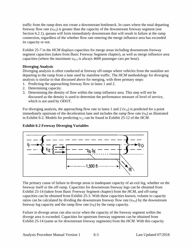
For diverging analysis, the approaching flow rate in lanes 1 and 2 (v12) is predicted for a point immediately upstream of the deceleration lane and includes the ramp flow rate (vR) as illustrated in Exhibit 6-2. Models for predicting v12 can be found in Exhibit 25-12 of the HCM. Exhibit 6-2 Freeway Diverging Variables
The primary cause of failure in diverge areas is inadequate capacity of an exit leg, whether on the freeway itself or the off-ramp. Capacities for downstream freeway legs can be obtained from Exhibit 25-14 (taken from Basic Freeway Segment chapter) from the HCM, and off-ramp capacities can be obtained from Exhibit 25-3. With these capacities known, volume to capacity ratios can be calculated by dividing the downstream freeway flow rate (vFO) by the downstream freeway leg capacity and the ramp flow rate (vR) by the ramp capacity. Failure in diverge areas can also occur when the capacity of the freeway segment within the diverge area is exceeded. Capacities for upstream freeway segments can be obtained from Exhibit 25-14 (same as for downstream freeway segments) from the HCM. With this capacity

Analysis Procedure Manual Version 1 6-4 Last Updated 07/2018
known, a volume to capacity ratio can be calculated by dividing the freeway flow rate upstream of the diverge (vF) by the capacity of the upstream freeway segment. In addition to these conditions, the flow rate entering lanes 1 and 2 (v12) immediately upstream of the deceleration lane should be checked to see if it exceeds the maximum desirable level. A volume to capacity ratio for this area can be calculated by dividing the approaching flow rate (v12) by the maximum desirable flow rate of 4400 passenger cars per hour (Exhibit 25-14 of HCM). Unlike the other conditions described above, the condition where the flow rate entering lanes 1 and 2 exceeds the maximum desirable level may create locally high densities, but may not always result in freeway queuing because mainline traffic will typically shift into the outermost lanes to avoid the diverging traffic. Freeway queues are more likely to result in these situations where there are only two lanes for mainline traffic, forcing all vehicles to pass through the diverging area.
6.2.3 Weaving Segments
Weaving Configurations Another necessary step before the analysis can be conducted is the determination of the weaving type, which is based on the number of lane changes required of each weaving movement. The HCM methodology identifies three types of geometric configurations for weaving areas. Each of these types of configurations is described below, with diagrams provided in Exhibit 6-4.
• Type A: Weaving vehicles in both directions must make one lane change to successfully complete a weaving maneuver.
• Type B: Weaving vehicles in one direction may complete a weaving maneuver without making a lane change, whereas other vehicles in the weaving segment must make one lane change to successfully complete a weaving maneuver.
• Type C: Weaving vehicles in one direction may complete a weaving maneuver without making a lane change, whereas other vehicles in the weaving segment must make two or more lane change to successfully complete a weaving maneuver.
Typically weaving segments are formed when merge areas are followed closely by diverge areas (within 2,500 feet) and the two are joined by an auxiliary lane requiring the crossing of two or more traffic streams traveling in the same general direction along a significant length of highway without the aid of traffic control devices. Note that when one-lane on-ramps are followed by one-lane off-ramps and the two are not connected by an auxiliary lane, weaving analysis is not conducted and the merge and diverge areas are analyzed independently using the procedures previously described. Recognition of configurations that could result in weaving is critical in highway operations analysis, as weaving areas require intense lane changing maneuvers that create a significant amount of turbulence. ODOT prefers the use of the HCM methodology for analyzing weaving maneuvers, but also supports the use of the Leisch Method in cases where engineering judgment suggests HCM results are not accurately reflecting conditions. For weaving areas greater than 2,500 feet use the more conservative of either the merge/diverge or Leisch methods. The HCM discusses weaving concepts in Chapter 13 and the analysis methodology in Chapter 24. While most analysts will take advantage of the practicality of the Highway Capacity Software (HCS), which will perform all needed calculations to analyze weaving areas, it is
Analysis Procedure Manual Version 1 6-5 Last Updated 07/2018
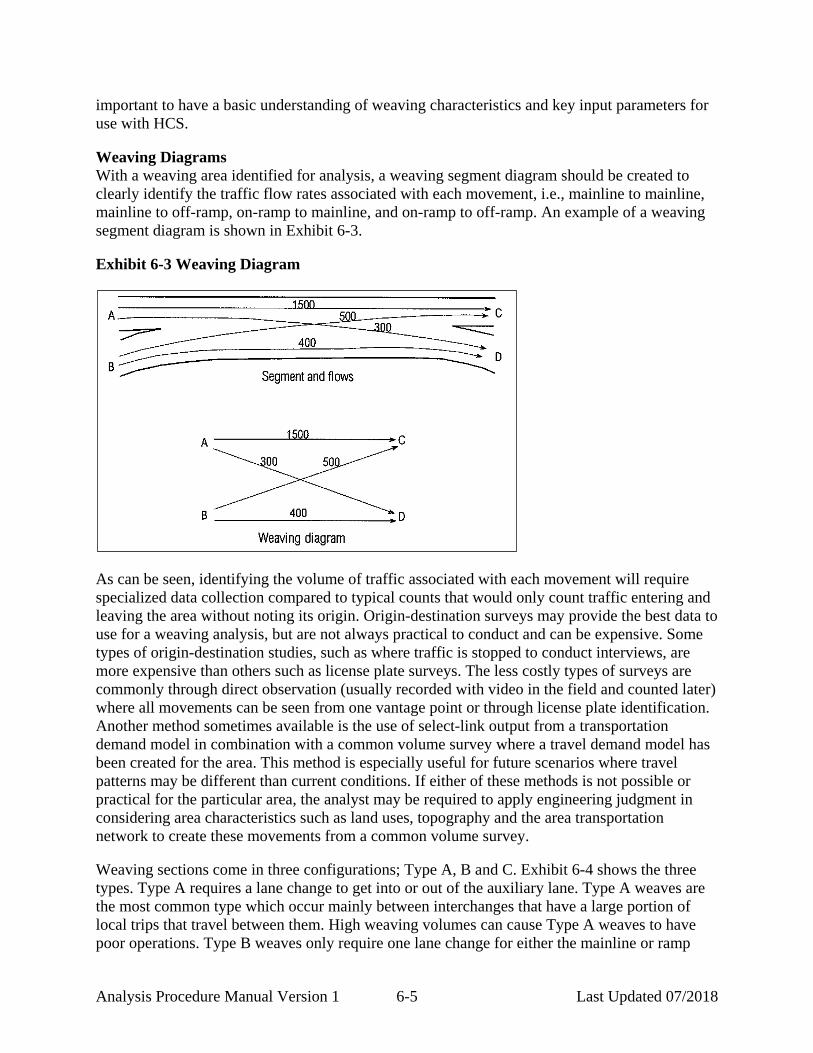
important to have a basic understanding of weaving characteristics and key input parameters for use with HCS. Weaving Diagrams With a weaving area identified for analysis, a weaving segment diagram should be created to clearly identify the traffic flow rates associated with each movement, i.e., mainline to mainline, mainline to off-ramp, on-ramp to mainline, and on-ramp to off-ramp. An example of a weaving segment diagram is shown in Exhibit 6-3. Exhibit 6-3 Weaving Diagram
As can be seen, identifying the volume of traffic associated with each movement will require specialized data collection compared to typical counts that would only count traffic entering and leaving the area without noting its origin. Origin-destination surveys may provide the best data to use for a weaving analysis, but are not always practical to conduct and can be expensive. Some types of origin-destination studies, such as where traffic is stopped to conduct interviews, are more expensive than others such as license plate surveys. The less costly types of surveys are commonly through direct observation (usually recorded with video in the field and counted later) where all movements can be seen from one vantage point or through license plate identification. Another method sometimes available is the use of select-link output from a transportation demand model in combination with a common volume survey where a travel demand model has been created for the area. This method is especially useful for future scenarios where travel patterns may be different than current conditions. If either of these methods is not possible or practical for the particular area, the analyst may be required to apply engineering judgment in considering area characteristics such as land uses, topography and the area transportation network to create these movements from a common volume survey. Weaving sections come in three configurations; Type A, B and C. Exhibit 6-4 shows the three types. Type A requires a lane change to get into or out of the auxiliary lane. Type A weaves are the most common type which occur mainly between interchanges that have a large portion of local trips that travel between them. High weaving volumes can cause Type A weaves to have poor operations. Type B weaves only require one lane change for either the mainline or ramp

Analysis Procedure Manual Version 1 6-6 Last Updated 07/2018
movement. These do not "trap" vehicles in the weaving section, so speeds are higher and operate much better than Type A weaves. Type C weaves require more than one lane change to perform the weaving maneuver and generally only operate well if the movement that must change lanes multiple times has a small volume. Type C weaves are relatively uncommon, are generally discouraged, but may exist in older highway alignments.

Analysis Procedure Manual Version 1 6-7 Last Updated 07/2018
Exhibit 6-4 Weaving Configurations
Type A Configuration
Type B Configuration
Type C Configuration
Type A ConfigurationType A Configuration
Type B ConfigurationType B Configuration
Type C ConfigurationType C Configuration

Analysis Procedure Manual Version 1 6-8 Last Updated 07/2018
Constrained vs. Unconstrained Conditions Applying the weaving methodology, other geometric characteristics must be described including whether the weaving area is operating under constrained or unconstrained conditions and identifying the length of the weaving area. The determination of whether a weaving segment is operating under constrained or unconstrained conditions is based on the relationship between the number of lanes that must be used by weaving vehicles to achieve equilibrium with non-weaving vehicles (NW) and the maximum number of lanes that can be used by weaving vehicles for a given configuration (NW(max)). Where NW < NW(max), conditions are described as unconstrained because there are no impediments to weaving vehicles’ ability to achieve equilibrium with non-weaving traffic. Where NW > NW (max), conditions are considered to be constrained because weaving vehicles are not provided enough roadway width as would be needed to reach equilibrium. Under constrained operation weaving vehicles often experience operating conditions much worse than those experienced by non-weaving vehicles, while under unconstrained conditions weaving and non-weaving vehicles usually experience similar operating conditions. The calculation of NW and NW(max) is determined by the configuration type, i.e., Type A, B, or C, and speeds of weaving and non-weaving vehicles. See Exhibit 24-7 in the HCM. When using the HCS to perform calculations, the analyst will only be required to determine the configuration type, free-flow speed and total number of lanes in the weaving section. However, an understanding of the characteristics of constrained and unconstrained conditions is important when analyzing weaving areas. Weaving Length Because weaving vehicles must execute all lane changes between the entry and exit gores, weaving lengths are measured from a point at the merge gore where the right edge of the freeway shoulder lane and the left edge of the merging lane are 2-feet apart to a point at the diverge gore where the two edges are 12-feet apart. Weaving lengths are limited to 2,500 feet in the HCM methodology. For weaving areas greater than 2,500 feet, use the more conservative of either the merge/diverge or Leisch methods. Weaving Density The key element of the HCM weaving analysis methodology is the calculation of the weaving area density, which is determined by incorporating weaving characteristics such as flow rate, configuration and free-flow speed. For a complete description of the density calculation refer to Chapter 24 of the HCM. The HCM uses the performance measure of level of service to rate weaving operations, which is directly related to the density calculated according to Exhibit 6-5.

Analysis Procedure Manual Version 1 6-9 Last Updated 07/2018
Exhibit 6-5 Level of Service Criteria for Weaving Segments
Level of Service
Density (Passenger Cars/Mile/Lane)
Freeway Weaving Segment Multi-Lane and Collector-
Distributor* Weaving Segments
A < 10.0 <12.0 B 10.0 – 20.0 12.0 – 24.0 C 20.0 – 28.0 24.0 – 32.0 D 28.0 – 35.0 32.0 – 36.0 E 35.0 – 43.0 36.0 – 40.0 F >43.0 >40.0
* See page 24-19 of the HCM – research is unclear on applicability of LOS criteria to collector-distributor roads. Weaving Capacity While ODOT does not use level of service for evaluating facility performance, the density of the weaving section is still used to determine the volume to capacity ratio. If the capacity of the weaving section is equated to the level of service E/F threshold shown in Exhibit 6-5, then the capacity of a freeway weaving section would occur at a density of 43 passenger cars per mile per lane. The capacity in passenger cars per hour at this density can be found through the following iterative process. 1. Complete the analysis using the HCM methodology. While this methodology will produce a
level of service, which is not needed, it will also produce a density. 2. The capacity of the weaving section will be equal to the total entering flow rate that results in
a calculated density of 43 passenger cars per mile per lane (for freeways). Using the flow rates from the initial analysis, begin an iterative process by multiplying each movement flow rate by a common factor until the resulting density reaches, but does not exceed, 43 passenger cars per mile per lane.
3. Add the individual movement flow rates that produced the target density to obtain the total entering flow rate, which will be taken as the weaving section capacity.
The volume to capacity ratio for the section can now be calculated by dividing the original total entering flow rate by the capacity (total entering flow rate resulting in target density). This process of iteration will typically require fewer than ten attempts. The same procedure can be used for weaving analysis of non-freeway facilities, but a different target density for the capacity will be required, as shown in Exhibit 6-5 for multi-lane and collector-distributor roadways. In addition to v/c ratio, the weaving section volume ration (VR) and speeds should be reported. The VR is the ratio of the weaving flow rate to the total flow rate. The HCM provides recommended upper limits on volume ratios. The difference between weaving and non-weaving speeds is a form of speed differential, which is preferred to be 10 mph or less for safety. Conditions exceeding these values should be examined using more detailed analysis methods such as simulation.

Analysis Procedure Manual Version 1 6-10 Last Updated 07/2018
Example 6-1 Weave Capacity Example
Given: Type A weave • 12 ft lanes • 6ft lateral clearance • 1000 ft weaving distance • 35 mph posted speed • Multilane highway segment
• 5% Trucks • PHF = 0.95 • Driver population factor = 0.95 • Volumes in vehicles per hour • Weaving and non-weaving flow
distributions Find: Volume-to-Capacity ratio for weaving section This example problem is based off of an actual project alternative. The lane and volume diagram shows the layout of the Type A weaving section and the volumes in vehicles per hour. The weaving section was created between a free-right turn at “B” and a loop off-ramp at “D” on a multilane roadway at an interchange. Lane and Volume Diagram
The lane volumes were converted into weaving (A-D and B-C) and non-weaving (B-D and A-C) volumes as shown below. In this case, future distributions were available from a cumulative analysis procedure. Other sources of weaving volumes include field collected origin-destination data such as by tracking vehicle license plates. Where a travel demand model is present, select link runs can help estimate weaving movements. Weaving Flow Diagram
The given information is then input into the HCM weaving procedure. The HCM result is a flow
1000 ft
C
BD
A
950
525
1235
240
1000 ft
C
BD
A
950950
525525
12351235
240240
A
D
C
B727
22317
508
A
D
C
B727
22317
508
Analysis Procedure Manual Version 1 6-11 Last Updated 07/2018
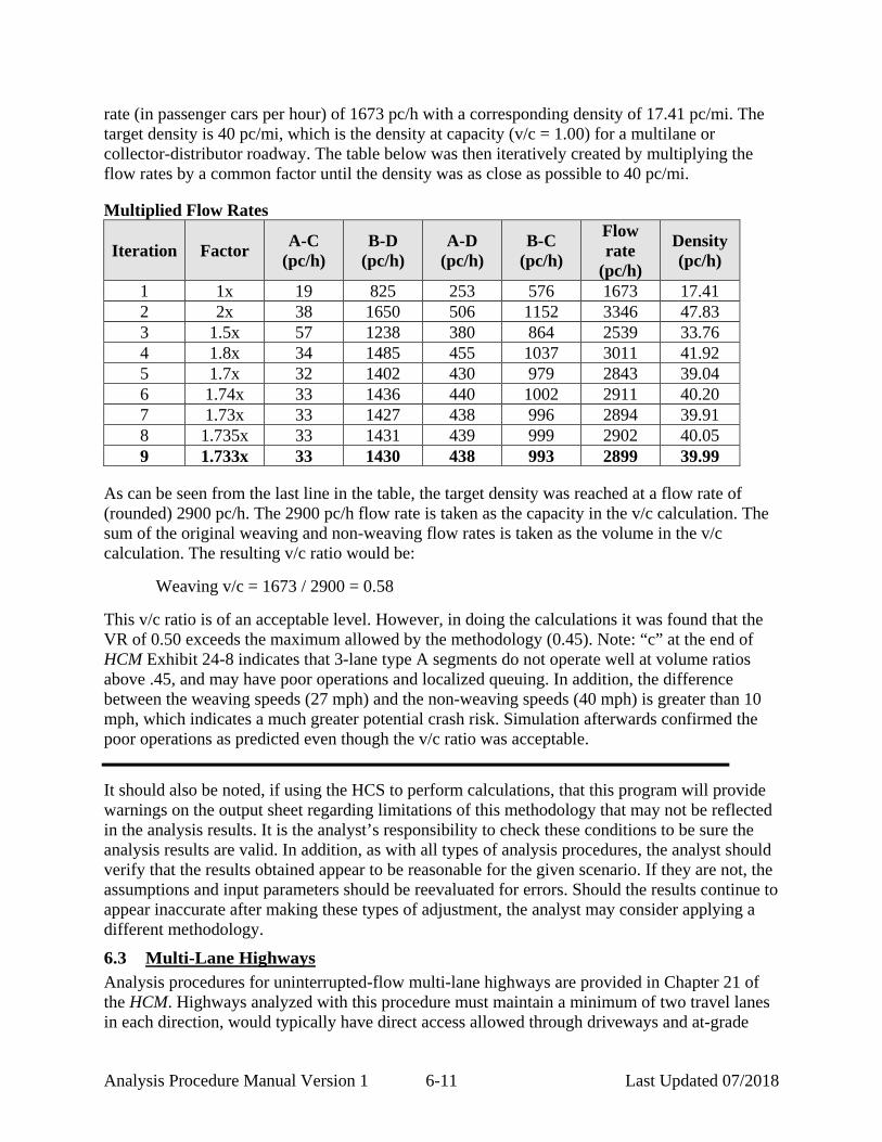
rate (in passenger cars per hour) of 1673 pc/h with a corresponding density of 17.41 pc/mi. The target density is 40 pc/mi, which is the density at capacity (v/c = 1.00) for a multilane or collector-distributor roadway. The table below was then iteratively created by multiplying the flow rates by a common factor until the density was as close as possible to 40 pc/mi. Multiplied Flow Rates
Iteration
Factor A-C
(pc/h) B-D
(pc/h) A-D
(pc/h) B-C
(pc/h)
Flow rate
(pc/h)
Density (pc/h)
1 1x 19 825 253 576 1673 17.41 2 2x 38 1650 506 1152 3346 47.83 3 1.5x 57 1238 380 864 2539 33.76 4 1.8x 34 1485 455 1037 3011 41.92 5 1.7x 32 1402 430 979 2843 39.04 6 1.74x 33 1436 440 1002 2911 40.20 7 1.73x 33 1427 438 996 2894 39.91 8 1.735x 33 1431 439 999 2902 40.05 9 1.733x 33 1430 438 993 2899 39.99
As can be seen from the last line in the table, the target density was reached at a flow rate of (rounded) 2900 pc/h. The 2900 pc/h flow rate is taken as the capacity in the v/c calculation. The sum of the original weaving and non-weaving flow rates is taken as the volume in the v/c calculation. The resulting v/c ratio would be:
Weaving v/c = 1673 / 2900 = 0.58 This v/c ratio is of an acceptable level. However, in doing the calculations it was found that the VR of 0.50 exceeds the maximum allowed by the methodology (0.45). Note: “c” at the end of HCM Exhibit 24-8 indicates that 3-lane type A segments do not operate well at volume ratios above .45, and may have poor operations and localized queuing. In addition, the difference between the weaving speeds (27 mph) and the non-weaving speeds (40 mph) is greater than 10 mph, which indicates a much greater potential crash risk. Simulation afterwards confirmed the poor operations as predicted even though the v/c ratio was acceptable. It should also be noted, if using the HCS to perform calculations, that this program will provide warnings on the output sheet regarding limitations of this methodology that may not be reflected in the analysis results. It is the analyst’s responsibility to check these conditions to be sure the analysis results are valid. In addition, as with all types of analysis procedures, the analyst should verify that the results obtained appear to be reasonable for the given scenario. If they are not, the assumptions and input parameters should be reevaluated for errors. Should the results continue to appear inaccurate after making these types of adjustment, the analyst may consider applying a different methodology.
6.3 Multi-Lane Highways Analysis procedures for uninterrupted-flow multi-lane highways are provided in Chapter 21 of the HCM. Highways analyzed with this procedure must maintain a minimum of two travel lanes in each direction, would typically have direct access allowed through driveways and at-grade
Analysis Procedure Manual Version 1 6-12 Last Updated 07/2018
intersections, and must maintain uninterrupted flow. Highways with access limited to on-ramps and off-ramps should be analyzed using the Basic Freeway Segment methodology. In addition, highways experiencing interrupted flow from influences such as traffic signals and on-street parking should be analyzed using a different methodology, such as the Urban Streets methodology from the HCM. These procedures are very similar to those previously described for basic freeway segments, with slightly different input data needs. The most notable differences include the need to account for median type and access density. For a complete description of the analysis methodology, refer to Chapter 21 of the HCM. While the HCM methodology uses level of service as a performance measure (based on vehicle density in passenger cars per mile per lane), volume/capacity ratios can be calculated from this analysis for comparison against ODOT’s adopted mobility standards by following the steps listed below. Note that separate volume/capacity ratios must be calculated for each direction of travel. 1. Assuming level of service E/F threshold represents capacity, determine the segment capacity
by interpolating between the values for “maximum service flow rate” at level of service E displayed in Exhibit 21-2 of the HCM for the appropriate free-flow speed. Free-flow speed will be either calculated by this methodology or assumed.
2. Divide the calculated flow rate (vp) by the interpolated capacity to obtain a volume/capacity ratio.
6.4 Two-Lane Highways – SEE APM VERSION 2 ADDENDUM 11B, Two-Lane Highways
6.4.1 Passing and Climbing Lanes
Both passing and climbing lanes are low-cost improvements that can be very effective in improving the operation of two-lane highways and can reduce the need to widen highways to four lanes. The HCM includes methodologies for analyzing these types of facilities in Chapter 20. When analyzing either passing or climbing lanes it must be determined whether a no-passing restriction will be placed on opposing traffic in the area of the added lane. If passing by opposing traffic will not be allowed, the operations of opposing traffic must be reanalyzed to include this restriction. While the methodologies described below can be used to evaluate the operations of passing and climbing lanes, the appropriate locations and lengths to use for design should be determined through the use of ODOT’s HDM. Passing Lanes Passing lanes are typically used where there may be inadequate passing opportunities, either because of sight distance limitations or as traffic volumes approach capacity. By providing a safe place to pass, passing lanes tend to reduce unsafe passing maneuvers. In addition to improving operations in the segment containing the passing lane, operations of the highway downstream of the passing lane may also be improved for up to several miles before queues begin to reform. Exhibit 20-23 in the HCM shows the general relationship between the directional flow rate and

Analysis Procedure Manual Version 1 6-13 Last Updated 07/2018
the length of the downstream roadway affected. The HCM methodology is applicable to directional segments of two-lane highways that include the entire passing lane, and should also include the full effective downstream length (Exhibit 20-23), if possible. A critical part of passing lane analysis using the HCM methodology includes dividing the analysis segment into four regions. 1. Upstream of the passing lane. 2. The passing lane, including tapers. 3. Downstream of the passing lane, but within its effective length. 4. Downstream of the passing lane, but beyond its effective length. When using the Highway Capacity Software (HCS) to perform calculations, only the total segment length, length upstream of the passing lane and length of the passing lane are needed for input. The program will automatically calculate the other lengths based on these lengths and the directional flow rate. As with the Two-Lane Highway analysis, a volume to capacity ratio for a directional segment must be obtained by dividing the passenger car equivalent peak 15-minute flow rate by the appropriate capacity. For a complete description of the remaining analysis assumptions and methodology, see Chapter 20 in the HCM. The analysis methodology in the HCM for passing lanes is intended to be applied to highways on level or rolling terrain only. Added lanes on mountainous terrain or on specific grades should be analyzed as climbing lanes. Climbing Lanes Climbing lanes are similar to passing lanes, but are generally used where grades cause unreasonable reductions in operating speeds of some vehicles. An unreasonable reduction in operating speeds is typically considered to occur where speed differentials of more than 10 mph are created. These lanes increase the capacity of a two-lane highway by providing a specific lane for slower vehicles to travel in while climbing an extended grade. This enables faster vehicles to pass these slower vehicles safely without having to leave the main travel lane. While climbing lanes are typically thought of as being associated with upgrades, they can also be applied to downgrades where heavy vehicles must drive in a low gear to avoid speeding out of control. When analyzing the downgrade direction, passenger car equivalents for trucks operating at crawl speeds are available in Exhibit 20-18 of the HCM. For all other heavy vehicles, the passenger car equivalents in the HCM for level terrain should be used (Exhibit 20-9).

Analysis Procedure Manual Version 1 7-1 Last Updated 07/2018
7 INTERSECTION ANALYSIS – SEE APM VERSION 2 CHAPTERS 12 AND 13

Analysis Procedure Manual Version 1 8-1 Last Updated 07/2018
8 TRAFFIC SIMULATION MODELS
8.1 Purpose Traffic simulation models are complex tools that can provide valuable information on the performance and potential improvement of transportation systems. Traffic simulation models are in a constant state of improvement and accordingly this chapter attempts to be adaptive with the changes in the industry. This chapter currently presents instruction on calibration of microsimulation models created in Trafficware’s SimTraffic and a brief overview of the other simulation models and parameters used in ODOT projects. Topics covered include:
• Traffic Simulation Modeling – General Calibration Instructions • SimTraffic – Overview and Calibration Instructions • VISSIM – Overview • Paramics - Overview • CORSIM – Overview
8.2 Traffic Simulation Modeling – General Calibration Instructions Traffic simulation models are computer programs that simulate traffic movements over a user-defined transportation network and present the results via animation and reports. The degree of user control over the simulation and the types of facilities that can be modeled will vary depending on the program being used. These should not be confused with urban travel demand models (Section 4.6), which use current and projected land use and transportation network data to estimate current and future travel demand and traffic patterns. Traffic simulation models (meso or microscopic) are complex tools that generally require more labor than programs that perform capacity analysis at a macro level. Because of this, they are generally only used when the use of other types of analysis tools will not be adequate for a given project. Simulation models offer a greater degree of flexibility than most programs designed specifically for capacity analysis and can be used for a wide range of analysis needs such as examining the interactions between different modes of transportation, modeling the operations of HOV lanes or bus priority systems and evaluating operations through measures of effectiveness not offered by most other types of analysis programs. Simulation models are also very useful for presentations, especially for those given to audiences lacking technical knowledge of traffic analysis, because it provides a visual basis for evaluating operations that most people can easily relate to and understand. Simulation models are commonly used by ODOT to analyze corridors or networks under congested conditions, where upstream or downstream operations have a significant influence on actual intersection operations (e.g., intersection blockage from queue spillback). It should be noted that simulation models use different methodologies for estimating queue lengths than other procedures described in this manual. These methodologies are typically based on observations of queues experienced during simulation, which are influenced by parameters such as driver characteristics, lane changing behavior and various traffic flow interactions. Capturing the impact of up and downstream operations on vehicle queues can make these models very effective at estimating queue lengths, but underscores the importance of good model calibration. General

Analysis Procedure Manual Version 1 8-2 Last Updated 07/2018
guidelines for the application of simulation models have been published by the Federal Highway Administration, which can be found at the FHWA website under traffic analysis tools. Depending on the specific program used, there may be numerous parameters that can be manipulated by the user to create a system that most accurately represents the one being analyzed. Before any simulation model is used to represent existing or future conditions, the existing conditions model created must be calibrated by adjusting operational parameters until the model provides a reasonable representation of existing conditions measured in the field. Existing conditions need to be replicated; otherwise future conditions will not be correct. Existing conditions should include only data, operations and measures known to currently exist in the project study area. Vehicle counts should be kept as close as possible to the original volumes obtained from the field. If all counts are available from the same day, vehicle counts used during calibration should be un-factored and unbalanced counts (this day should be as close to the 30th highest hour as possible). If counts cannot all be collected on the same day (or year), every effort should be made to collect counts at primary locations on a day that is on or closely represents, the 30th highest hour. The remaining counts can then be factored and balanced to this primary count day. If all counts occur on scattered days and none of the counts occur on the 30th highest hour or on a representative day then short sample count should be conducted to factor the off- peak counts to the day the study area was visited. Use the seasonal factor methodology described in Section 4.4 to determine if the count is close enough to the 30th highest hour. If the primary counts for the study area occurred during a time that is less than 90% of the 30th highest hour for that area seasonal trend type, then a re-visit with a sample count is required for the calibration of the “existing” model. These rules are established to help ensure that calibration volumes 1) are near the 30th highest hour and 2) represent conditions that have been witnessed in the field. The emphasis is placed on witnessed, as the analyst needs to visit the study area on or near the count day (30th highest hour) so that the visual check of the simulation (the first step in calibration) is based on conditions that occurred in the field during the count. The Field Inventory Worksheet shows all the measures from the field that should be input into the simulation and visually checked in the animation to help analysts in the data collection process. In Chapter 3, Transportation System Inventory, Exhibit 3-2 shows an example completed worksheet for a simulation project. Note that the worksheet is intended to be printed multiple times for a given project area. The collection of worksheets can be placed in a three-ring binder providing a hard writing surface. Each copy of the worksheet can be used for each intersection or area of interest in the study and all copies can be neatly organized in a single project binder (see Exhibit 3-1). The site visit should occur as close as possible to the 30th highest hour. After the site a calibration scenario can be constructed. For the purpose of calibration, the peak hour volumes from the counts should be seasonally adjusted to the time period of the site visit. The calibration network should include all measurements taken and all operational behavior witnessed. Many of the behavioral issues should be collected on the worksheet provided above. For Synchro and SimTraffic inputs refer to Sections 7.3.9 and 8.3. These sections refer specifically to Synchro/SimTraffic, but the list provided should include most of the measures that would have to be checked or adjusted in any software platform. Note that most microsimulations go into greater detail than SimTraffic, so there will likely be more measures to check and adjust. Also note that illegal behavior such as speeding, improperly using medians or shoulders as turn bays

Analysis Procedure Manual Version 1 8-3 Last Updated 07/2018
and improper lane changing distances should be accounted for in during calibration, but should not be continued to be assumed in the future build scenarios. All non-calibration alternative analysis should assume that all drivers follow the rules of the road. Once the “existing” inputs and behavior is coded into the simulation software, the analyst should run an animation to visually check the reasonability of the microsimulation. Any gross error like queues or blockages being much greater or much less than the field observations should be addressed by re-checking inputs. Further refinement may include measuring and adjusting saturation flow rates, driver reaction time and travel speed. A good place to start is by comparing simulated vehicle queues to those visually observed in the field. For some corridors, comparing simulated travel times or average speeds to actual observed conditions may be appropriate. Good calibration is not only critical for accurate analysis, but will establish credibility during presentations with technical advisory committees or public groups that have prior knowledge of existing problem areas. Exhibit 8-1 illustrates how the calibration process fits into the complete analysis. The calibration, existing and site visit hour refer to the same hour. In other words, the “calibration” data is collected in the study area in the “site visit” hour to represent “existing” conditions. For further information on calibration in general, consult the FHWA Analysis Toolbox. Section 8.3 has the detailed procedures on calibrating a SimTraffic model using SimTraffic for ODOT projects. Exhibit 8-1 Simulation Construction and Application Flow Chart
May need to bring headway factors and posted speed back to
defaults – Engineering Judgment
If needed
Raw CountsAnnual Adjustments
Seasonal Factors
Annual AdjustmentsSeasonal Factors
Likely to be needed
Annual AdjustmentsFuture Path Adjustments
Calibration Hour“Existing” Hour Visit Site Hour
Field Measurements: Headway, Free-Flow Speed
Engineering JudgmentCalibrated Using “Vehicles
Exited” for SimTraffic
30th Highest Hour Volumes
Build or Analysis Year Volumes

Analysis Procedure Manual Version 1 8-4 Last Updated 07/2018
8.3 SimTraffic
8.3.1 Overview
SimTraffic performs microsimulation and animation of vehicle traffic, modeling travel through signalized and unsignalized intersections and arterial networks, as well as freeway sections, with cars, trucks, pedestrians and buses. SimTraffic includes the vehicle and driver performance characteristics developed by the Federal Highway Administration for use in traffic modeling. They were developed for CORSIM and Trafficware used them as they were published. Most of the input is entered through the Synchro program, but some parameters, such as the driver and vehicle characteristics, are modified through SimTraffic specifically. SimTraffic can be used for all ODOT plans, projects and traffic impact studies. SimTraffic is primarily used by ODOT for the analysis of signal systems and vehicle queue estimation, especially in congested areas and locations where queue spillback may be a problem. For the estimation of signalized vehicle queues, SimTraffic is generally preferred in Regions 2 through 5 where v/c ratios exceed 0.70 and in Region 1 where v/c ratios exceed 0.90, but should always be used where v/c ratios exceed 0.90. SimTraffic should typically be used for the analysis of all coordinated signal systems. For isolated intersections, Synchro and SimTraffic should provide similar results. SimTraffic results will differ from Synchro most when the v/c ratio exceeds 0.90, when there are closely spaced intersections and other conditions that are not ideal. Overcapacity queues and metering conditions are identified in Synchro’s Timing Window with a “#” or “m” symbol.
8.3.2 Simulation Calibration
As much as possible, operational field data should be obtained for the major facilities in the study area as close as possible to the design hour (see Appendix H). Beyond the field data listed in Section 3.2, additional field measures may be needed to achieve calibration of the microsimulation. If needed, saturation flow studies should be performed at the major intersections. Floating car travel time runs may need to be performed to ensure that observed and simulated travel times (and related speeds) are close. Free-flow link speeds using road-tube counters or speed guns (RADAR, LIDAR, etc) may need to be collected and used in place of posted speed limits during calibration. At the very least, the existing conditions network needs to be visually calibrated to the field conditions and the “vehicles exited” measure from SimTraffic should be reviewed. If everything is close, then the SimTraffic simulation should duplicate conditions seen in the field. Congested and free-flow areas in the field should be congested and free-flowing in the simulation. If there is more congestion in the simulation than in the field, then one or more parameters may be off. For example, saturation flows and resulting headway factors may be too low, counts may be balanced too high, peak hour factors may be too low, link and turning speeds may be low, storage bays and taper lengths may be too short and intersection paths and lane change distances may be incorrect. If congestion is too low then the reverse of these may be a cause. To help determine the cause of inconsistencies with known conditions, any number of measures
Analysis Procedure Manual Version 1 8-5 Last Updated 07/2018
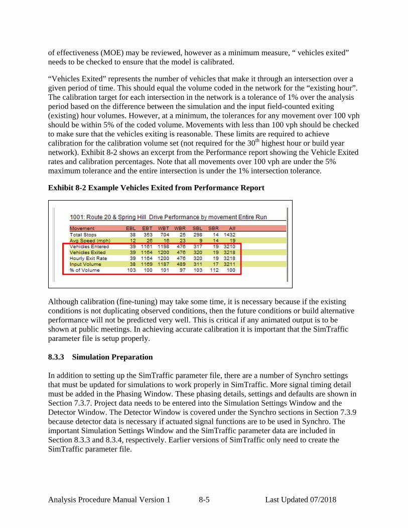
of effectiveness (MOE) may be reviewed, however as a minimum measure, “ vehicles exited” needs to be checked to ensure that the model is calibrated. “Vehicles Exited” represents the number of vehicles that make it through an intersection over a given period of time. This should equal the volume coded in the network for the “existing hour”. The calibration target for each intersection in the network is a tolerance of 1% over the analysis period based on the difference between the simulation and the input field-counted exiting (existing) hour volumes. However, at a minimum, the tolerances for any movement over 100 vph should be within 5% of the coded volume. Movements with less than 100 vph should be checked to make sure that the vehicles exiting is reasonable. These limits are required to achieve calibration for the calibration volume set (not required for the 30th highest hour or build year network). Exhibit 8-2 shows an excerpt from the Performance report showing the Vehicle Exited rates and calibration percentages. Note that all movements over 100 vph are under the 5% maximum tolerance and the entire intersection is under the 1% intersection tolerance. Exhibit 8-2 Example Vehicles Exited from Performance Report
Although calibration (fine-tuning) may take some time, it is necessary because if the existing conditions is not duplicating observed conditions, then the future conditions or build alternative performance will not be predicted very well. This is critical if any animated output is to be shown at public meetings. In achieving accurate calibration it is important that the SimTraffic parameter file is setup properly.
8.3.3 Simulation Preparation
In addition to setting up the SimTraffic parameter file, there are a number of Synchro settings that must be updated for simulations to work properly in SimTraffic. More signal timing detail must be added in the Phasing Window. These phasing details, settings and defaults are shown in Section 7.3.7. Project data needs to be entered into the Simulation Settings Window and the Detector Window. The Detector Window is covered under the Synchro sections in Section 7.3.9 because detector data is necessary if actuated signal functions are to be used in Synchro. The important Simulation Settings Window and the SimTraffic parameter data are included in Section 8.3.3 and 8.3.4, respectively. Earlier versions of SimTraffic only need to create the SimTraffic parameter file.

Analysis Procedure Manual Version 1 8-6 Last Updated 07/2018
8.3.4 Simulation Settings Window
The following data is only used by SimTraffic and needs to be included for a proper simulation. This data allows for geometric refinement and operational behavior of the simulation. The data required by SimTraffic should be a part of the field collection/observation process and is included the Field Inventory Worksheet.
• Storage Length (ft) – The Storage Length is the length of a turning bay from the stop bar to the beginning of the taper. Storage Length is the area that can store vehicles and does not include tapers. If the Left or Right Turn lane goes all the way back to the previous intersection, enter "0". Storage Length data is used for analyzing potential blocking problems. Storage length is typically field measured or estimated from aerial photographs. If measurements are unknown or if the facility is new, the initial storage lengths of 100’ for urban and 150’ for rural can be used. SimTraffic outputs will be used to refine these lengths for build alternatives.
• Taper Length (ft) – The Taper Length is the remaining length of the turning bay from the end of the storage length to where the outer edge of the turning bay meets the outer edge of the adjacent lane. This value is field-measured or estimated from aerial photographs. For state highways, the taper lengths can be obtained from the Highway Design Manual Figures 8-8 for right turn lanes and 8-9 for left turn lanes. This allows turning bays to store several more vehicles and allows a truer and a more consistent (with design) representation.
• Lane Alignment – The Lane alignment controls the vehicle paths in SimTraffic. When links are constructed, Synchro shows either a “Left” or “Right” alignment as default. This may not be correct especially if multilane approaches, skewed intersections, short links, free-flow ramp connections and merge/diverge/weaving sections make up a particular intersection.
Other choices are “L-NA” and “R-NA” which will force the vehicle path either left or right. To check the lane alignment, the Intersection Paths box must be checked under the Map Settings window. The default color or zoom level will likely need to be changed to clearly see the paths. Exhibit 8-3 shows that Synchro defaults to single-lane turn lanes turning into a multilane leg with paths going to either departing lane. Unless lines are marked on the pavement guiding vehicles into different lanes Oregon vehicular code states that vehicles need to turn into the nearest lane. In most of these cases the Lane Alignment needs to be changed to “L-NA” or “R-NA” depending on the turn type.

Analysis Procedure Manual Version 1 8-7 Last Updated 07/2018
Exhibit 8-3 Default Lane Alignment
For the existing calibrated network, the legal setting may not need to be followed if the majority of field-observed vehicles turn into both lanes (although itself an improper lane choice). Design alternatives should be always be coded legally. Note that the northbound dual left turn lane shown in Exhibit 8-3 has the correct paths. The southbound left still needs to be changed to limit traffic to the inside through lane. In cases of acceleration lanes, merging traffic should be forced right using “R-NA” and through traffic forced left using “L-NA.” This will keep through vehicles out of the acceleration lane.
• Enter Blocked Intersection – This setting controls whether mainline or side-street traffic can enter a blocked intersection. In earlier versions of SimTraffic, vehicles did not block intersections. Default is “No” for intersections and “Yes” for bend nodes and ramp junctions. This factor is best obtained through field observation.
Along many busy roadways, minor intersections and driveways are frequently blocked by through traffic, so in this case the setting should be “Yes” for the through traffic. If “Do Not Block Intersection” signs exist, then the setting should remain “No” unless the signs are generally ignored. If there are intersections or accesses that are frequently blocked and through vehicles let side street vehicles out, then the side street movements can be set to “1 veh” which will allow one vehicle to enter. Use of the “2 veh” setting has a tendency to cause the simulation to clog up.
• Link Offset (ft) – The Link Offset is used to set the roadway left or right of the natural centerline. This is typically used in creating “dogleg” or offset intersections without

Analysis Procedure Manual Version 1 8-8 Last Updated 07/2018
creating a second node. • Crosswalk Width (ft) - this is the width of the crosswalk on an approach. This setting
controls the placement of the stop bar which controls detector placement and link length. ODOT default crosswalk width is 12 feet (outside edge to outside edge) unless the adjoining sidewalk is wider. Local intersections should be measured.
• Headway Factor - The saturation flow rate in SimTraffic for intersection approaches is adjusted through the Headway Factor. The saturated flow rate calculated in Synchro is not used in SimTraffic; however, the corresponding headway factor is automatically calculated. In simulation calibration, the headway factor can be adjusted to help fine-tune (calibrate) the SimTraffic simulation. Exhibit 8-4 shows the equivalent headway factor for a given saturated flow rate. Earlier versions of Synchro/SimTraffic need to have the headway factor manually calculated in the Lane Window.
Exhibit 8-4 Headway Factors
Headway Factor Saturated Flow Rate 1.2 1650 vphpl 1.1 1750 vphpl 1.0 1850 vphpl 0.9 2050 vphpl 0.8 2250 vphpl
• Turning Speed (mph) – This is the turning speed used by SimTraffic by movement. Higher speeds will increase the capacity of the SimTraffic simulation. Synchro default is 15 mph for left turns and 9 mph for right turns. The 9 mph right turn speed is too slow unless used for turning onto residential local streets or in a downtown central business district location.
ODOT default is 15 mph for left and right turns. Non-standard turns at skewed intersections, channelized turns and interchanges should have different values and can be estimated by recording speeds while driving through the subject intersections or using a speed gun to capture turning vehicle speeds. Turning speeds are also needed for merge/diverge sections at interchanges or bend nodes.
• Lane Change Distances - Changes to these calculated values can help calibrate the vehicle lane-changing operation. Changes may be necessary if vehicles are having difficulty completing lane changes ahead of intersections or off-ramps or if vehicles are artificially clogging up at lane drops after an intersection or a two-lane ramp merging into a single lane. High heavy vehicle percentages combined with a higher amount of long vehicles and/or a congested network increases the chances that modifications will be required. Closely spaced intersections will have short lane change distances while interchanges will have longer lane change distances as many drivers move into the desired lane considerably ahead of an off-ramp. The analyst will need to experiment with these values, either longer or shorter until the traffic is flowing consistent to the observed conditions or flowing smoothly for future conditions. Modifying ramp geometry so that the ramps enter the mainline as turns rather than as a straight-through movement makes for smoother operation and less need to modify these distances.

Analysis Procedure Manual Version 1 8-9 Last Updated 07/2018
There are two different types of lane change distances: mandatory and positioning. The Mandatory Distance is the distance measured from the stop bar at which a lane change must occur. The Positioning distance is the distance measured back from the Mandatory Distance where a vehicle first attempts a lane change. The Mandatory and Position Distance 2’s are extra distance added if a second lane change is necessary. All of these distances can extend around corners. Adding to the challenge of changing these variables, is that the driver types in SimTraffic have a range of a 50% (aggressive) to a 200% (passive) multiplier to the set distances.
8.3.5 SimTraffic Parameter File
The SimTraffic parameter file controls the simulation operation and the defaults must be changed to reflect the proper impacts of queuing, travel time, etc. The parameter file has three major sections: Vehicles, Drivers and Intervals. The TPAU Analysis Tools webpage has a default SimTraffic template file with all of the basic parameters set up. The following shows the variables that need to be changed. All other settings are left unchanged. The Vehicles tab controls the type and physical vehicle characteristics.
• Vehicle Occurrence (%) - SimTraffic uses the Synchro heavy vehicle percentage to simulate the total number of heavy vehicles relative to all vehicles. When the simulation calls for a heavy vehicle, the vehicle type is represented by this factor which represents the percentage breakout of the global truck fleet. Likewise, when a car is called for, this factor will split the car types among the global car fleet percentages.
o Earlier versions of SimTraffic defaulted to having the total vehicle percentages sum up to 100%.
o SimTraffic 7 defaults total up to 100% for the car fleet and 100% for the truck (includes buses) fleet as shown in Exhibit 8-5.
o Change the Vehicle Occurrence (%) for the different vehicle classes to match the composite average of your classification counts. If classification counts are unavailable, state highway vehicle classification segment data (available at https://highway.odot.state.or.us/cf/highwayreports/traffic_parms.cfm) can be used substituted. Average between multiple counts at the project boundaries and on different significant facilities both state and local. Note that while the heavy vehicle percentages per approach may vary largely, the heavy vehicle mix does not vary as much. The total truck fleet should total up to 100% and the total car fleet should total up to 100%. Car1 represents the larger passenger vehicles in the fleet (i.e. SUV’s, large
pickups); Car2 represents smaller passenger vehicles in the fleet; TruckSU represents single unit trucks (i.e. delivery vans, dump trucks); SemiTrk1 represents single tractor-trailer combinations; SemiTrk2 represents shorter single tractor-trailer combinations; Truck DB represents trucks with two trailers; Note: SemiTrk2 and Truck
DB can be customized to fit other truck types like triple trailers. Bus represents buses in the fleet; Carpool1 & Carpool2 represents vehicles with the same characteristics as
Car1 and 2 but with higher occupancies. Zero out the default Carpool1 and

Analysis Procedure Manual Version 1 8-10 Last Updated 07/2018
Carpool2 vehicles. These will have no effect on the simulation unless vehicle occupancy is used as an evaluation measure.
Exhibit 8-5 SimTraffic Default Vehicle Parameters
• Vehicle Length (ft) – This parameter directly affects queuing distances. Leaving the length unchanged will result in the queues being underestimated. Change the vehicle length in the following vehicle types:
o Car1 = 20 ft; o Car2 = 16 ft; o TruckSU = 30 ft; o SemiTrk1 = 75 ft.
The Drivers tab (Exhibit 8-6) controls the behavior characteristics for the 10 different driver types that make up the simulation from the passive to the aggressive. For example, Driver Type 1 has 15% lower link speeds and will take 200% more distance when making a lane change while Driver Type 10 will travel 15% faster than the link speed and have lane change distances 50% of the coded values. All of the factors in the Drivers tab remain the same with exception of the Green React (s) setting. This setting reflects the time from when the signal turns green to the time that the vehicle begins to move. This value can be captured in the field and used as a calibration parameter. TPAU research indicates that Oregon values are substantially different than the defaults in SimTraffic. Change the Green React times to match Exhibit 8-7.
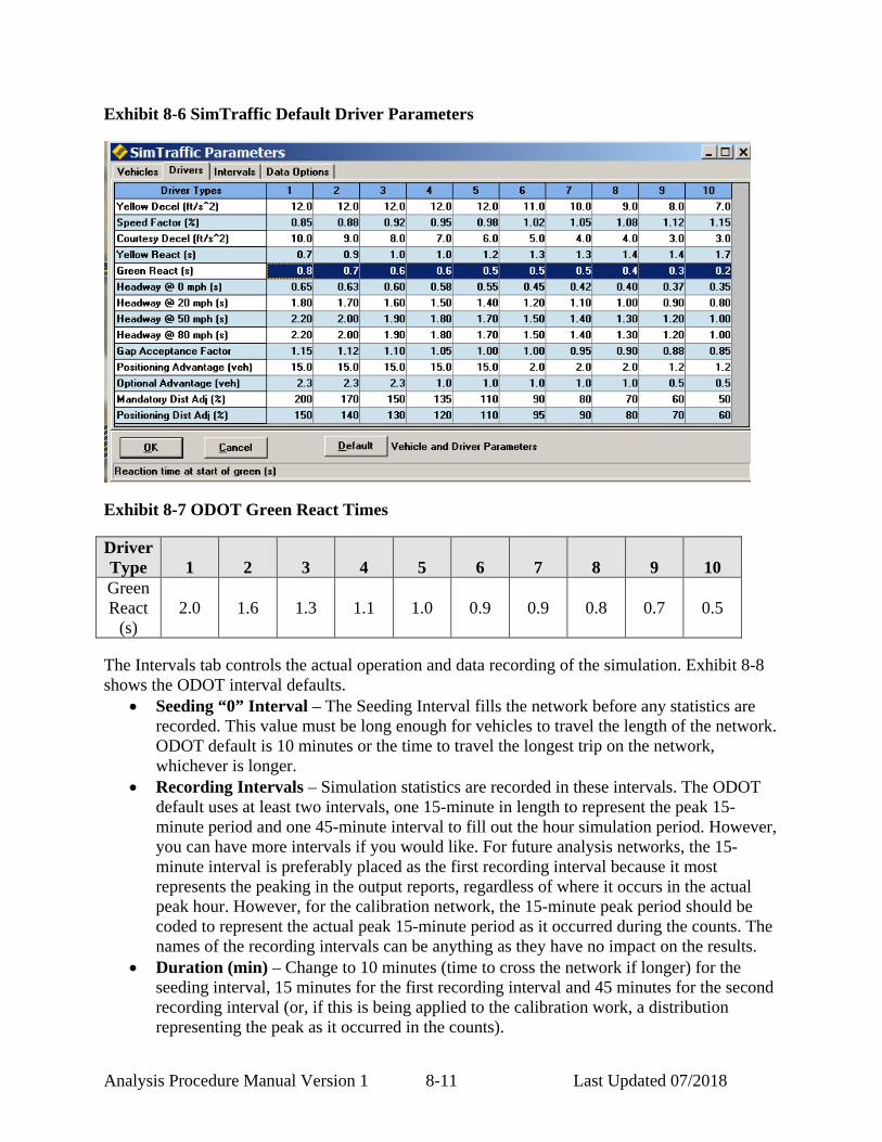
Analysis Procedure Manual Version 1 8-11 Last Updated 07/2018
Exhibit 8-6 SimTraffic Default Driver Parameters
Exhibit 8-7 ODOT Green React Times
Driver Type
1
2
3
4
5
6
7
8
9
10
Green React
(s)
2.0
1.6
1.3
1.1
1.0
0.9
0.9
0.8
0.7
0.5
The Intervals tab controls the actual operation and data recording of the simulation. Exhibit 8-8 shows the ODOT interval defaults.
• Seeding “0” Interval – The Seeding Interval fills the network before any statistics are recorded. This value must be long enough for vehicles to travel the length of the network. ODOT default is 10 minutes or the time to travel the longest trip on the network, whichever is longer.
• Recording Intervals – Simulation statistics are recorded in these intervals. The ODOT default uses at least two intervals, one 15-minute in length to represent the peak 15-minute period and one 45-minute interval to fill out the hour simulation period. However, you can have more intervals if you would like. For future analysis networks, the 15-minute interval is preferably placed as the first recording interval because it most represents the peaking in the output reports, regardless of where it occurs in the actual peak hour. However, for the calibration network, the 15-minute peak period should be coded to represent the actual peak 15-minute period as it occurred during the counts. The names of the recording intervals can be anything as they have no impact on the results.
• Duration (min) – Change to 10 minutes (time to cross the network if longer) for the seeding interval, 15 minutes for the first recording interval and 45 minutes for the second recording interval (or, if this is being applied to the calibration work, a distribution representing the peak as it occurred in the counts).

Analysis Procedure Manual Version 1 8-12 Last Updated 07/2018
• Start Time (hhmm) – After Duration is specified, change the start time to reflect the hour being simulated.
• Record Statistics – Set to “Yes” for all recording intervals. • Growth Factor Adjust – Set to “Yes” for all intervals. • PHF Adjust & AntiPHF Adjust – The combination of these two settings creates a spike
in the simulated hour. The PHF Adjust should be set to “Yes” during the seeding and the peak 15-minute intervals and the AntiPHF Adjust set to “No.”. The AntiPHF Adjust should be set to “Yes” and the PHF Adjust set to “No” for all other recording intervals.
• Percentile Adjust - Set to “No” for all intervals. Use of this setting will overestimate the queuing in the simulation.
• Random Number Seed – SimTraffic uses nine different simulation scenarios (1 through 9). If it is desired to produce duplicate results, select a non-zero setting. ODOT default is to set it to ‘0’ which will produce random arrival rates with each run.
Exhibit 8-8 ODOT Intervals Defaults
8.3.6 Simulation Execution
Once all Synchro and SimTraffic settings are completed, the simulation is ready to be executed. Upon starting the simulation, the “Errors and Warnings” window will appear. This shows anything that is outside of the value ranges what SimTraffic expects to find. Errors are split into fatal and non-fatal errors. Fatal errors will not allow the simulation to run and must be corrected. Fatal errors usually are related to lanes and lane groups where no lanes exist on a link. Non-fatal errors still allow a simulation to be run, but these need to be reviewed and corrected if possible for best results. Some examples of non-fatal errors that need to be corrected are:
• “Detector too close to stop bar” ; • Minimum green /total split/pedestrian timing errors;

Analysis Procedure Manual Version 1 8-13 Last Updated 07/2018
• Reference phase not in use errors; • Storage lane and length errors.
Some examples of non-fatal errors that can be left alone as these are “how it is” are:
• “Angle between approaches less than 25 degrees.” Small angles will lengthen out an intersection area and may cause unpredictable operation.
• Any error referencing vehicle extensions or minimum gaps exceeding 111% of travel time between detectors. Errors such as these indicate that actuated signal operation will be not as efficient.
• “Volume-delay operation not recommended with long detection zone.” SimTraffic has issues generally with ODOT’s default phasing variables.
ODOT standard is to average together at least five (5) random acceptably working (no system gridlock) runs. If you have a congested or a large network, it is advisable to have 7-10 runs to allow for “blown” runs which are caused by system gridlock so there are at least five good runs averaged together at the end. The system gridlock is typically caused by the improper actions of simulated vehicles that end up getting stuck. If every run or a majority of runs have gridlock, then the analyst should further refine the simulation settings, especially the headway factors, blocked intersection and lane change distance parameters. It can take 20-40 minutes a run (depending on network size, congestion level and computer speed). Make sure you have adequate available storage. Each simulation file can be in excess of 1 GB. If you run out of space during a multiple recording session, SimTraffic will continue to run, but the simulations will stop being recorded. Once the runs are completed, check each simulation run by selecting each number in the drop-down run number box to make sure it is free of any system gridlock errors and that the simulation reflects what is expected. If there are bad runs, make note of the run number, so it may be skipped in the report process.
8.3.7 Simulation Outputs
SimTraffic outputs are used for queue analysis, determination of storage lane lengths, travel times and other evaluation criteria. Many times in the evaluation of alternatives the typical v/c and LOS measures may have very small differences. It is common practice today to use additional MOE’s to describe an operation of an alternative. These MOE’s can include travel time, stopped delay, average speed and queue blocking. These are very useful in alternative comparisons because lower travel times, delays and stops coupled with higher average speeds, will indicate a more operationally efficient alternative. Make sure before selecting any report to print or preview that a number is showing in the run number box. Otherwise, a message appears from SimTraffic saying that it needs to record the simulation again. To preview a report, select the desired report(s) and make sure that the Multiple Runs box is checked. Select the desired .hst files (skipping any bad runs). Reports are generally broken down into sections by intersection and interval. The Summary of All Intervals section of the report is

Analysis Procedure Manual Version 1 8-14 Last Updated 07/2018
where information is pulled from for analysis. Check to make sure that content, headers and footers are correct before printing.
• Simulation Summary Report – Used to check whether that the runs look to have similar characteristics. Entering and exiting vehicles, total delay and total stops should be relatively consistent between runs. This is a second check of the run adequacy (the first is visual inspection). This report also gives system total MOE’s which can be used in alternative comparisons.
• Queuing and Blocking Report - The Queuing and Blocking report generates the 95th percentile queues which are used to design turn bay storage as well as document operation of the study area. Exhibit 8-9 shows a typical report.
This report shows three different queues: maximum, average and 95th. The reported maximum queue is the highest queue calculated every two minutes. The average queue (50th percentile) is the average of the calculated two-minute queues. The 95th Queue is the 95th percentile of the reported maximum queue over the simulated period. With the Random Number Seed set to zero, the queues in this report will be different from those in another set of simulation runs. When reporting out the estimated queue lengths, round up to the next 25 feet.

Analysis Procedure Manual Version 1 8-15 Last Updated 07/2018
Exhibit 8-9 Sample Queuing and Blocking Report
The Upstream Block Time and the Storage Block Time are of particular interest in helping describe the overall impact of queuing. While the 95th percentile queues may show how long a queue is, the block time shows for how long of the simulated hour the queue will block intersections or storage bays. Even if queue spillback into adjacent intersections is not occurring, storage bays may be overflowing, causing local problems such as the blockage of adjacent lanes. A queue blockage or spillback condition is considered a problem when the duration exceeds five (5) percent of the peak hour. Spillback may also be a sign of cycle failure as there may not have been enough green time available to serve all waiting vehicles. Signals do not recover instantly, so one spillback cycle could affect the operation of the next two or three cycles which can be a significant portion of hourly cycles.
• Upstream Blk (Block) Time (%) - This is an estimated percentage of the peak hour in which the queue from the subject node blocks an upstream node. This is especially useful when analyzing a complex Synchro network, to determine the extent of queuing on a system when reporting out results. It can also be used to determine if an alternative or option will provide the best progression.
• Storage Blk (Block) Time (%) - This reports an estimated percentage of the peak hour

Analysis Procedure Manual Version 1 8-16 Last Updated 07/2018
in which the length of the through or turning queues exceeds the storage length. For build analysis, if your storage block time is significant (>5%), then it is recommended to enter a longer bay length, rerun the simulation and continue this until you get a percentage less than 5%. Keep in mind that storage bays should adhere to the practical limit of 300 – 350 feet (most storage bays are 100 to 150 feet), so some alternatives and their simulations will still have significant storage block time.
Queues can be reported directly from the subject approach if the queue length is less than the link length. If a queue is longer than the link length, then the total actual queue length will be the link length(s) that are completely filled up plus the last queue length that does not exceed the link length. The analyst will need to trace the queue back from the intersection in question, so you will likely pass though multiple intersections and bend nodes to obtain the actual queue length. However, this queue is made up of contributions from other intersections that the subject queue spills back into which can make it hard to tell and report where exactly the queue originates. Queues are best reported graphically by identifying the queues under spillback conditions separately from the ones that do not exceed the link length. Exhibit 8-10 shows a sample 95th percentile queuing diagram. To minimize reporting issues, link curvature should be used where possible to eliminate any unnecessary bend nodes. The combination of the upstream and storage block times can also be used to report out the impacts of queuing at a higher level instead of reporting out the 95th percentile queues for intersection approaches. Exhibit 8-10 Sample Queuing Diagram
OREGON DEPARTMENT OF TRANSPORTATION
File : Fern Valley.ppt
Date : 2/25/2005
TRANSPORTATION PLANNING ANALYSIS UNITTPAU
Fern Valley Interchange - 2004 30th Highest Hour No-Build 95th Percentile Queues FIGURE 3Prepared By: C. Fera-Thomas
Rev. By: P. Schuytema PE
Pear Tree Ln.
N. Phoenix Rd.
Fern Valley Rd.
Cheryl L
n.
I-5
OR 99
E. Bolz Ln.
Bear Creek
Luman Rd.
NORTHNO SCALE
W. Bolz L
n.
S. Phoenix Rd.
Luman Rd.
100’ 250’
275’
50’
200’
325’75’
100’
550’
650’
700’
650’
950’
100’175’
375’
50’
150’
= Isolated 95th Percentile Queues= Overlapping intersection 95th Percentile Queues
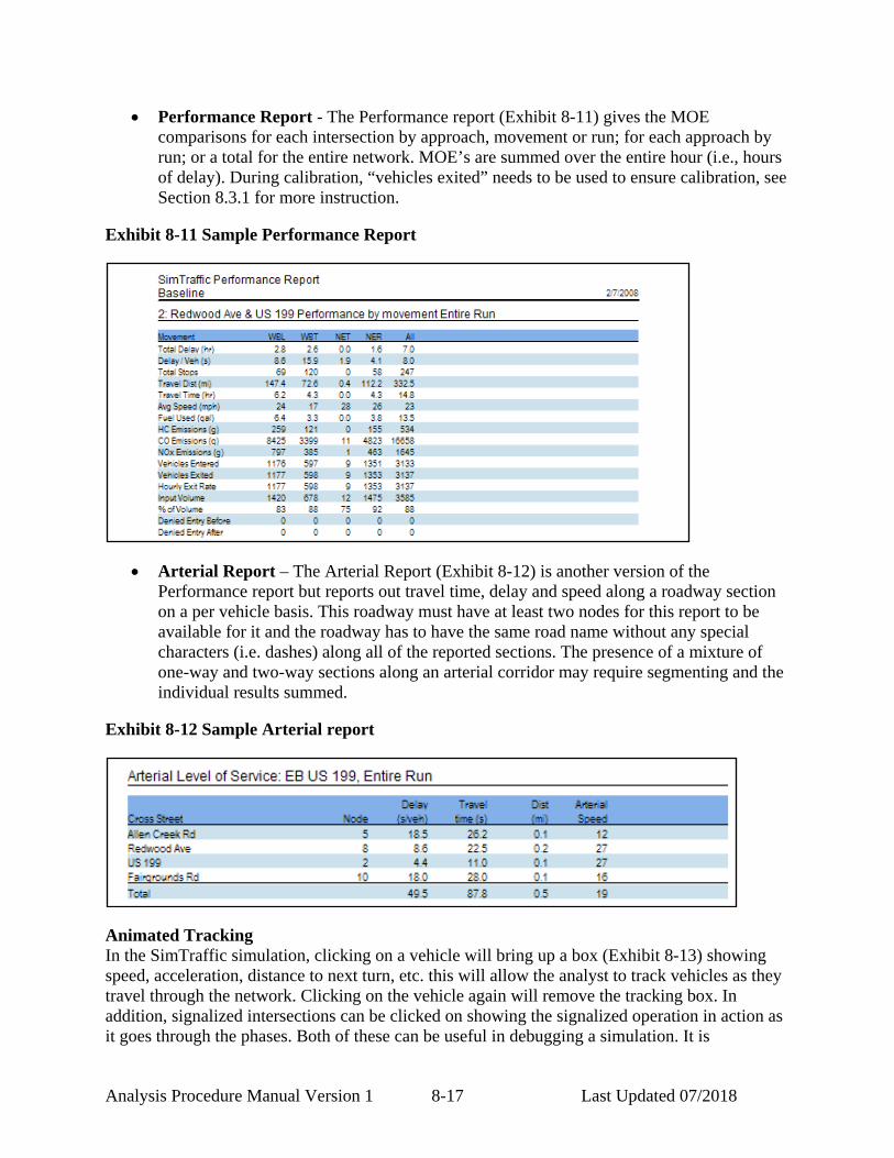
Analysis Procedure Manual Version 1 8-17 Last Updated 07/2018
• Performance Report - The Performance report (Exhibit 8-11) gives the MOE comparisons for each intersection by approach, movement or run; for each approach by run; or a total for the entire network. MOE’s are summed over the entire hour (i.e., hours of delay). During calibration, “vehicles exited” needs to be used to ensure calibration, see Section 8.3.1 for more instruction.
Exhibit 8-11 Sample Performance Report
• Arterial Report – The Arterial Report (Exhibit 8-12) is another version of the Performance report but reports out travel time, delay and speed along a roadway section on a per vehicle basis. This roadway must have at least two nodes for this report to be available for it and the roadway has to have the same road name without any special characters (i.e. dashes) along all of the reported sections. The presence of a mixture of one-way and two-way sections along an arterial corridor may require segmenting and the individual results summed.
Exhibit 8-12 Sample Arterial report
Animated Tracking In the SimTraffic simulation, clicking on a vehicle will bring up a box (Exhibit 8-13) showing speed, acceleration, distance to next turn, etc. this will allow the analyst to track vehicles as they travel through the network. Clicking on the vehicle again will remove the tracking box. In addition, signalized intersections can be clicked on showing the signalized operation in action as it goes through the phases. Both of these can be useful in debugging a simulation. It is

Analysis Procedure Manual Version 1 8-18 Last Updated 07/2018
recommended that the simulation speed be set to real time or slower for best viewing. Exhibit 8-13 Animated Vehicle and Signal Tracking
Static Graphics Other reports include the “Static Graphics” reports (Exhibit 8-14). Select the Graphics tab and you will get a box showing reports such as total delay, percent time blocked queues, etc. These reports are based on the same information that the previous comprehensive reports use, but display the information in graphical form, rather than a table of numbers. These report out just the run number selected rather than an average of runs of the regular reports. These can be use to quickly visualize the issues for the analyst or for others.

Analysis Procedure Manual Version 1 8-1 Last Updated 07/2018
Exhibit 8-14 Example Queue Length Static Report
8.4 Vissim - Overview Vissim is a simulation program that can model multi-modal traffic flows including cars, trucks, buses, heavy rail and light rail transit (LRT) as well as model traffic management systems (ramp meters, toll roads, and special lanes) and transit priority systems. Vissim can also model trip assignment, over fixed routes or dynamically, where vehicles change routes in response to specified events and can animate traffic movements in 3-D. Vissim is a program that can stand alone, but is data intensive to create files for use on its own. Alternatively, the files can be created in Visum (a travel demand program) that can then import the files into Vissim for analysis. See APM version 2 Appendix 8B for guidance on creating networks using PTV Vision Suite software (Visum, Vissim, and Vistro). Because most ODOT region offices do not perform travel demand modeling, it is important to note issues both with and without Visum. Other advantages of Vissim include the rail-roadway interface, which requires Vissim Level 3 or 4 in order to model the effect of rail crossing blockages on queues and roadway operations. Another advantage is that Vissim has the capability of “dynamic traffic assignment” (DTA), which will reroute a vehicle on the network in case of a crossing blockage or an overcapacity situation. Note that this strength of the software comes at the price of larger study areas to allow for correct dynamic assignment and to address effects occurring potentially outside of the focus of the study area. DTA will likely require more data, measures and resources to properly calibrate (see APM version 2 Chapter 8 for more information). APM version 2 Addendum 15A is a link to the ODOT Vissim Protocol which governs documentation and creation of all Vissim models created for ODOT plans and projects.

Analysis Procedure Manual Version 1 8-2 Last Updated 07/2018
Vissim has the capability of performing analysis directly on Visum traffic volume assignments and includes a post-processing function. The results of this type of analysis may be acceptable for certain applications, such as sketch planning and alternative screening. However, for most types of analysis, DHVs are required. The function in Vissim does not create DHVs, therefore the post-processing procedures outlined in APM version 2 Chapter 6 are still necessary. Most ODOT region offices do not currently own the Vissim software (outside of Region 1). The ODOT Synchro defaults should be implemented in the Vissim model to the extent possible. Most region offices outside of Region 1 are unlikely to have the knowledge base to use Visum.
8.5 Paramics - Overview Paramics and VISSIM share a lot of the same benefits in functionality and issues with complexity and time to achieve calibration. Paramics, like VISSIM, is a simulation program that can model multi-modal traffic flows including cars, trucks, buses, heavy rail and light rail transit (LRT) as well as model traffic management systems (ramp meters, toll roads and special lanes) and transit priority systems. Paramics can also model trip assignment, over fixed routes or dynamically, where vehicles change routes in response to specified events and can animate traffic movements in 3-D. Paramics is a program that can stand alone, but is data intensive to create files for use on its own. Paramics does offer some importing functionality to bring networks in from other software, but it does not have a direct link to VISUM. However, all of Paramics’ inputs are text files, making it easy to customize automations (macros, scripts, etc.) to take networks from other platforms and format the data into the text files Paramics requires. This creates many opportunities to bring networks from any software quickly into Paramics. Arguably the biggest strength of any dynamic assignment software (like Paramics and VISSIM) is the “dynamic traffic assignment” (DTA) option, which will reroute a vehicle on the network in case of a rail crossing blockage or an overcapacity situation. Note that this strength of the software comes at the price of larger study areas to allow for correct dynamic assignment and to address effects occurring potentially outside of the focus of the study area. DTA will likely require more data, measures and resources to properly calibrate. Paramics has disadvantages similar to VISSIM since it does not produce signal coordination timing and can be very data intensive and time consuming to construct and calibrate a scenario, especially from scratch. Some issues to consider when using Paramics for analysis are (based on ODOT’s assessment of version 5.2):
• The flexibility of Paramics means the analyst is required, in most cases, to write their own reports. Paramics does have a set of limited standardized reports. This would require exporting the queuing data to Excel or comparable software; creating functions to calculate the maximum queues for each time period, calculating averages and standard deviations and then calculating the 95th percentile queue on each approach for each run.
• Paramics does not do signal coordination/progression, so the network must be constructed in Synchro (or similar software) to develop the timing and progression, which can then be incorporated into Paramics.
• Paramics should not be used in a TIS process as there are too many parameters to change

Analysis Procedure Manual Version 1 8-3 Last Updated 07/2018
and is likely out of the capable review range of most Region analysts. • To date, none of the ODOT offices own the Paramics software. Paramics submittals by
consultants should include the Paramics model translated into Synchro files to enable effective ODOT review. The ODOT Synchro defaults should be implemented in the Paramics model to the extent possible.
Currently, Paramics is not practical enough for most ODOT applications. Model development is data intensive, requires detailed knowledge on many input parameters and has limited standardized output reports. The use of Paramics input text file format can speed up some of the work but requires a custom import/export process which can be very time consuming to develop.
8.6 CORSIM - Overview CORSIM is a microscopic traffic simulation program, applicable to surface streets, freeways and integrated networks with a complete selection of control devices, i.e., stop/yield sign, traffic signals and ramp metering. CORSIM simulates traffic and traffic control systems using commonly accepted vehicle and driver behavior models and combines two traffic simulation models: NETSIM for surface streets and FRESIM for freeways. CORSIM allows for user control of trip assignment through the ability to set vehicle-type specific turn percentages and set predefined vehicles routes.

Analysis Procedure Manual Version 1 9-1 Last Updated 07/2018
9 DETERMINING NEEDS – SEE APM VERSION 2 CHAPTER 9

Analysis Procedure Manual Version 1 10-1 Last Updated 07/2018
10 ANALYZING ALTERNATIVES – SEE APM VERSION 2 CHAPTER 10

Analysis Procedure Manual Version 1 11-1 Last Updated 07/2018
11 AIR AND NOISE TRAFFIC DATA
11.1 Purpose Federal regulation requires, in some cases, that an air and noise study be completed to determine what impact, if any, will result from a proposed highway improvement and what measures will be taken to lessen these impacts. This chapter presents the general outline for the needs and processing of common data requested for the Air and Noise Analysis section of the Environmental Impact Statement (EIS) or Environmental Assessment (EA). Topics covered include:
• Input for Noise Analysis • Input for Air Quality Analysis • EISBase
11.2 Input for Noise Analysis ODOT is responsible for ensuring that state transportation projects are developed within the Federal Highway Administration’s noise policies and procedures. To conduct the noise analysis necessary for measuring compliance, the ODOT Geo-Environmental Section, or noise consultant, requires specific data from the project traffic analyst. This request is typically made through the Noise, Air and Energy Traffic Requirements Check List, which is filled out by the noise consultant or Geo-Environmental Section staff and delivered to the project traffic analyst. While this list identifies many different types of possible data needs, the collection and processing of the most common data requested is discussed below. This process should only be done on the No-Build and Selected Alternatives because of the time required to complete the work. Typically it will take a month for the no-build and a bit less for each build alternative.
11.2.1 Common Data Needs
The traffic data requested will often be required for a no-build condition under the existing year, the year of opening and the future design year (typically 20 years from opening) as well as for build conditions for each alternative being considered under the year of opening and the future design year. At the beginning of the project, 16-hour manual full federal (13 vehicle classes) classification turn movement counts need to be ordered at all signalized intersections in addition to all intersections with substantial traffic volumes or heavy vehicle movements. Shorter duration counts can be used at minor intersections between the classification count locations. These counts are also used to develop the traffic volumes for the project. See Chapter 4. The factors that are created from count data are based on the peak hour, the average hour, the average daily traffic, and the peak truck hour, which cannot be calculated from a peak period count. There will need to be enough classification counts so passenger car, medium and heavy vehicle movements can be calculated at the shorter duration count locations. Be sure to request an electronic version of all count data in spreadsheet format to aid in data processing.

Analysis Procedure Manual Version 1 11-2 Last Updated 07/2018
The first step in the noise data process should be the creation of link diagrams depicting the study area roadway segments that will be included in the analysis for all no-build and build scenarios considered. These diagrams are not only useful for graphically relating the data provided to its location, but help in identifying links created, modified, or removed with each alternative. Each link should be given a unique number for identification purposes. It should be noted that the link number can be directional. Directional link numbers should be provided for freeways, expressways, interchanges, one-way streets, couplets, divided highways and facilities with separate roadbeds. Where possible, try to keep consistent numbering between the no-build and build link diagrams. This will mean adding extra links that have zero data into the no-build network that will accommodate the build Alternative. The more consistent the diagrams are, the easier it will be for the traffic analyst to troubleshoot and the noise analyst to follow. There is nothing wrong with having links with no data in the scenarios as long as they are labeled as not existing yet or not existing anymore. A set of sample link diagrams is provided in Exhibit 11-1. Exhibit 11-1 Sample Link Diagram – Jackson School Road Interchange
The second step is recording the specific link characteristics, which include street name, length (in miles), posted speed and LOS C volume. Link length is the center-to-center intersection spacing. Links on the edge of the network should have a length of 0.25 mile. Speeds recorded for this analysis should be either the posted speed limit or the operating speed (highest overall speed at which a driver can travel on a given highway under favorable weather conditions and under prevailing traffic conditions, without at any time

Analysis Procedure Manual Version 1 11-3 Last Updated 07/2018
exceeding the safe speed as determined by the design speed on a section-by-section basis) where it is determined to be consistently higher than the posted speed limit. Directional interim LOS C volumes for each link can be assumed to be as follows:
• For freeway segments, obtain from the latest version of the HCM. For example, in the HCM 2000 the LOS C volume for a basic freeway segment with a free-flow speed of 60 mph would be 1560 pcphpl. The LOS C volume is calculated using the HCM delay methodologies, via an iterative process based on the project volumes, to identify the volume where the LOS C threshold occurs (at the top end of LOS C, adjacent to LOS D). Use the following defaults only for links at the end of the network.
• For freeway ramps, assume 1000 pcphpl. The analyst should consider effects of ramp metering on freeway ramp LOS C volumes, where applicable.
• For urban arterials, assume 600 pcphpl. • For suburban arterials, assume 700 pcphpl. • For rural highways, assume 800 pcphpl.
In noise analysis, the LOS C volume is assumed to represent the maximum volume that can be sustained at free-flow speed. Because vehicle speeds typically affect noise levels more than vehicle volumes, this condition is often the most critical. In areas where peak period congestion is minimal or only occurs for a short time, allowing for continuously high speeds, the peak hour or peak truck hour may be critical. However, in areas where congestion is present for extended periods, lowering vehicle speeds, the LOS C volume may have a greater impact.
11.2.2 Calculations
When the count data ordered becomes available it will be necessary to regroup the 13 vehicle classes into the medium, heavy and all vehicles categories for the noise analysis. Noise sources associated with transportation projects can include passenger vehicles, medium trucks, heavy trucks and buses. Each of these vehicles produces noise, however, the source and magnitude of the noise can vary greatly depending on vehicle type. For example, while the noise from passenger vehicles occurs mainly from the tire-roadway interface and is, therefore, located at ground level, the noise from heavy trucks is produced by a combination of noise from tires, engine and exhaust resulting in a noise source that is approximately 8-feet above the ground. The following list provides information on the types of transportation noise sources that will be part of a typical roadway project, and describes the type of noise each produces23.
• Passenger Vehicles: Noise emitted from 0 to 2 feet above roadway, primarily from tire-roadway interface. This category includes normal passenger vehicles, small and regular pickup trucks, small to mid-size sport utility vehicles and mini- and full-size passenger vans.
• Medium Trucks: Noise emitted from 2- to 5-feet above roadway, combined noise from tire-roadway interface and engine exhaust noise. This category includes delivery vans (e.g., UPS and Federal Express trucks) large sport utility vehicles
23 Traffic Noise Background Information, Michael Minor & Associates.
Analysis Procedure Manual Version 1 11-4 Last Updated 07/2018
with knobby tires, large diesel engine trucks, some tow-trucks, city transit and school buses with under vehicle exhaust, moving vans (U-Haul type trucks), small to medium recreational motor homes, and other larger trucks with the exhaust located under the vehicle. The federal vehicle classifications covered are: 2-axle other with trailer, 2-axle 6-tire single unit and buses. For practical application, include all trucks with 2 axles and 6 tires if insufficient information is available to provide for a more detailed analysis.
• Heavy Trucks: Noise emitted from 6- to 8-feet above the roadway surface, combined noise sources includes tire-roadway interface, engine noise and exhaust stack noise. This category includes all long-haul tractor-trailers (semi-trucks), large tow-trucks, dump trucks, cement mixers, large transit buses, motor homes with exhaust located at top of vehicle, and other vehicles with the exhaust located above the vehicle (typical exhaust height of 12- to 15-feet). The federal vehicle classifications covered are: 3-axle and greater single units and all combinations. For practical application, include all trucks with 3 or more axles.
NOTE: In reporting information on trucks the following criteria should be used:
• Truck tractor units traveling without a trailer will be considered single-unit trucks. • A truck tractor unit pulling other such units in a “saddle mount” configuration
will be considered one single-unit truck and will be defined only by the axles on the pulling unit.
• Vehicles are defined by the number of axles in contact with the road. Therefore, “floating” axles are counted only when in the down position.
• The term “trailer” includes both semi- and full trailers. The following are the federal classifications.
• Motorcycles (Optional): All two- or three-wheeled motorized vehicles. Typical vehicles in this category have saddle type seats and are steered by handlebars rather than steering wheels. This category includes motorcycles, motor scooters, mopeds, motor-powered bicycles and three-wheel motorcycles. This vehicle type may be reported at the option of the State.
• Passenger Cars: All sedans, coupes and station wagons manufactured primarily for the purpose of carrying passengers and including those passenger cars pulling recreational or other light trailers.
• Other Two-Axle, Four-Tire Single Unit Vehicles: All two-axle, four-tire vehicles, other than passenger cars. Included in this classification are pickups, vans and other vehicles such as campers, motor homes, ambulances, hearses, carryalls and minibuses. Other two-axle, four-tire single-unit vehicles pulling recreational or other light trailers are included in this classification. Because automatic vehicle classifiers have difficulty distinguishing class 3 from class 2, these two classes may be combined into class 2.
• Buses (Optional): All vehicles manufactured as traditional passenger-carrying buses with two axles and six tires or three or more axles. This category includes only traditional buses (including school buses) functioning as passenger-carrying vehicles. Modified buses should be considered to be a truck and should be appropriately classified.

Analysis Procedure Manual Version 1 11-5 Last Updated 07/2018
• Two-Axle, Six-Tire, Single-Unit Trucks: All vehicles on a single frame including trucks, camping and recreational vehicles, motor homes, etc., with two axles and dual rear wheels.
• Three-Axle Single-Unit Trucks: All vehicles on a single frame including trucks camping and recreational vehicles, motor homes, etc., with three axles.
• Four or More Axle Single-Unit Trucks: All trucks on a single frame with four or more axles.
• Four or Fewer Axle Single-Trailer Trucks: All vehicles with four or fewer axles consisting of two units, one of which is a tractor or straight truck power unit.
• Five-Axle Single-Trailer Trucks: All five-axle vehicles consisting of two units, one of which is a tractor or straight truck power unit.
• Six or More Axle Single-Trailer Trucks: All vehicles with six or more axles consisting of two units, one of which is a tractor or straight truck power unit.
• Five or Fewer Axle Multi-Trailer Trucks: All vehicles with five or fewer axles consisting of three or more units, one of which is a tractor or straight truck power unit.
• Six-Axle Multi-Trailer Trucks: All six-axle vehicles consisting of three or more units, one of which is a tractor or straight truck power unit.
• Seven or More Axle Multi-Trailer Trucks: All vehicles with seven or more axles consisting of three or more units, one of which is a tractor or straight truck power unit.
There may be times when data related to buses and motorcycles is requested to be provided separately. Separate motorcycle data is rarely needed in Oregon, but specific data related to bus volumes may be appropriate where the link could be experiencing higher than average bus traffic due to influence by a nearby school, bus barn, or tourist attraction. The count data can be regrouped by hand or by spreadsheet, however the process can be long and cumbersome. An easy way to process ODOT-counted 12-hour or greater counts is to request the count in electronic form in “TruckSum” format from the Transportation Systems Monitoring Unit. A copy of the spreadsheet is available on the TPAU website. This format organizes the count into the three basic subgroups of medium, heavy and all vehicles for the macro-based TruckSum Excel spreadsheet. See Exhibit 11-2 and Exhibit 11-3, which calculates the initial truck factors. Note: The Exhibit margins were cut off due to a software issue. The TruckSum spreadsheet calculates for each intersection leg the peak hour volume, the average daily traffic, the average daily truck volume, the average 8-hour volume and the peak truck hour volume. The spreadsheet also calculates the necessary truck factors explained later in this section. The analyst either types the summarized count values into the spreadsheet or copies and pastes the TruckSum-formatted count data into the spreadsheet. Use Paste – Special Values only, to avoid corrupting the output. The analyst also enters the length of the manual count (12 hours minimum), count date and location. Pressing the “Calculate” button on the spreadsheet will generate the factors and the rest of the data (page two of the output). It is best to print out the spreadsheet in landscape

Analysis Procedure Manual Version 1 11-6 Last Updated 07/2018
format double sided. Note: A side benefit of this spreadsheet, if used early in the project, is that it can be used to help determine the overall peak hour of the study area as will as determining directional factors, K-factors (percent of daily traffic in the peak hour) and truck percentages for each leg.

Analysis Procedure Manual Version 1 11-7 Last Updated 07/2018
Exhibit 11-2 TruckSum Input
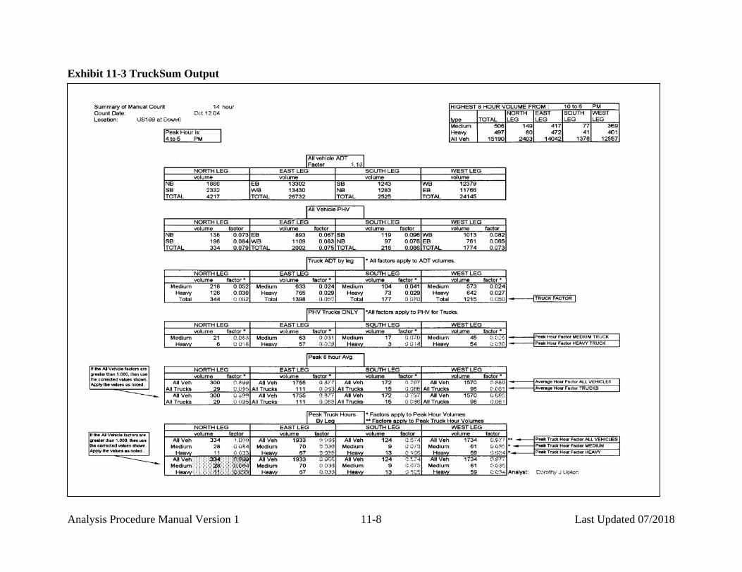
Analysis Procedure Manual Version 1 11-8 Last Updated 07/2018
Exhibit 11-3 TruckSum Output

Analysis Procedure Manual Version 1 11-9 Last Updated 07/2018
Average daily traffic (ADT) volumes and peak hour volumes (PHV) maintain the same meaning in noise analysis as they do in other types of analysis described in this manual. They are simply the total number of all vehicle types experienced on a link over a 24-hour period and the highest hourly total of all vehicle types experienced during that 24-hour period, respectively. Both of these must be documented for each link studied during all years and analysis scenarios requested. The “Truck Factor” represents the percent trucks in the average daily traffic volume, calculated as shown below.
The “Peak Hour Factor” for noise analysis, refers to the percent trucks in the peak hour of traffic for all vehicle types. This factor is usually needed for both medium and heavy vehicles separately and is calculated as shown below.
vehicles)all ofhour peak in vehicles(all vehicles)all ofhour peak in trucks(medium Factor,Hour Peak Trucks Medium =
vehicles)all ofhour peak in vehicles(all vehicles)all ofhour peak in cks(heavy tru Factor,Hour Peak TrucksHeavy =
Peak Truck Hour Factors refer to the percent of a specified vehicle type in the peak hour of all truck traffic. Most times the peak truck hour is different from the peak hour. These factors are typically calculated for all vehicle, medium truck and heavy truck classes, but the calculations for all vehicles is different than those for the truck classes. As an example, the peak truck hour factors for various classes are shown below.
vehicles)all ofhour peak in vehicles(allhour)peak truck allin vehicles(all Factor,Hour Truck Peak Vehicles All =
hour)peak truck allin vehicles(allhour)peak truck allin trucks(medium Factor,Hour Truck Peak Trucks Medium =
hour)peak truck allin vehicles(allhour)peak truck allin cks(heavy tru Factor,Hour Truck Peak TrucksHeavy =
Another type of factor that may be requested, though not often used, is the “Average Hour Factor.” This represents the percent of a specified vehicle type in an average 8-hour period and is commonly requested for the all vehicle types and all truck classes.
When bus or motorcycle traffic is requested separately, provide percentages of these vehicle types in the all vehicle peak hour and truck peak hour. For example, if providing bus data, the following calculations would be used:
vehicles)all ofhour peak in vehicles(all vehicles)all ofhour peak in (buses Hour Peak Vehicle Allin Buses % =
hour)peak truck allin vehicles(allhour)peak truck allin (buses Hour Peak Truck in Buses % =
vehicles)me of all -hour volu(trucks)me of all -hour volu( or Truck Fact
2424
=

Analysis Procedure Manual Version 1 11-10 Last Updated 07/2018
Note that while updated ADT and PHV values for each analysis year must be provided, only one set of TruckSum factors must be calculated for each alternative. It is generally assumed that while traffic volumes will increase over time, the proportion of vehicle types in the total volume will remain approximately the same. The factors in the TruckSum spreadsheet are for the indicated peak hour. Choose the peak hour that covers the most of the intersections. If the peak hour is different than the chosen hour, then the factors will need to be recalculated using the volumes for that hour. If buses are to be split out separately, then they will have to be done manually by splitting them from the medium trucks. The factors shown in boxes on the right side of the spreadsheet are described below with the related equations. Project wide peak hour adjustment using TruckSum
Often, different intersections on a project will have different peak hours. The peak hour calculated by TruckSum is the peak hour for each individual intersection. For those intersections where the peak hour is different from the system peak hour, the analyst can modify TruckSum to report the system peak hour, using the following procedure. TruckSum factors are calculated using the VLOOKUP function in the EXCEL spreadsheet. To calculate factors for a system peak instead of the intersection peak, the peak hour needs to be changed in the spreadsheet. Over-ride the VLOOKUP function by manually typing in the system peak hour in the peak hour cell. The spreadsheet will no longer choose the peak hour from the table and instead will use the selected hour.

Analysis Procedure Manual Version 1 11-11 Last Updated 07/2018
Step 1. Unprotect the worksheet as shown below.
Step 2. Change the peak hour to the system peak hour as shown on the following figure.

Analysis Procedure Manual Version 1 11-12 Last Updated 07/2018
Step 3. Observe revised peak hour volumes as shown on the following figures.
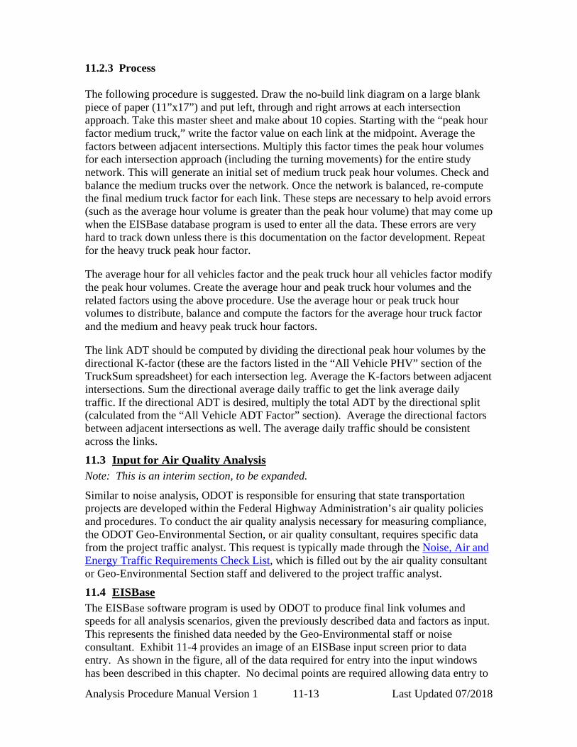
Analysis Procedure Manual Version 1 11-13 Last Updated 07/2018
11.2.3 Process
The following procedure is suggested. Draw the no-build link diagram on a large blank piece of paper (11”x17”) and put left, through and right arrows at each intersection approach. Take this master sheet and make about 10 copies. Starting with the “peak hour factor medium truck,” write the factor value on each link at the midpoint. Average the factors between adjacent intersections. Multiply this factor times the peak hour volumes for each intersection approach (including the turning movements) for the entire study network. This will generate an initial set of medium truck peak hour volumes. Check and balance the medium trucks over the network. Once the network is balanced, re-compute the final medium truck factor for each link. These steps are necessary to help avoid errors (such as the average hour volume is greater than the peak hour volume) that may come up when the EISBase database program is used to enter all the data. These errors are very hard to track down unless there is this documentation on the factor development. Repeat for the heavy truck peak hour factor. The average hour for all vehicles factor and the peak truck hour all vehicles factor modify the peak hour volumes. Create the average hour and peak truck hour volumes and the related factors using the above procedure. Use the average hour or peak truck hour volumes to distribute, balance and compute the factors for the average hour truck factor and the medium and heavy peak truck hour factors. The link ADT should be computed by dividing the directional peak hour volumes by the directional K-factor (these are the factors listed in the “All Vehicle PHV” section of the TruckSum spreadsheet) for each intersection leg. Average the K-factors between adjacent intersections. Sum the directional average daily traffic to get the link average daily traffic. If the directional ADT is desired, multiply the total ADT by the directional split (calculated from the “All Vehicle ADT Factor” section). Average the directional factors between adjacent intersections as well. The average daily traffic should be consistent across the links.
11.3 Input for Air Quality Analysis Note: This is an interim section, to be expanded.
Similar to noise analysis, ODOT is responsible for ensuring that state transportation projects are developed within the Federal Highway Administration’s air quality policies and procedures. To conduct the air quality analysis necessary for measuring compliance, the ODOT Geo-Environmental Section, or air quality consultant, requires specific data from the project traffic analyst. This request is typically made through the Noise, Air and Energy Traffic Requirements Check List, which is filled out by the air quality consultant or Geo-Environmental Section staff and delivered to the project traffic analyst.
11.4 EISBase The EISBase software program is used by ODOT to produce final link volumes and speeds for all analysis scenarios, given the previously described data and factors as input. This represents the finished data needed by the Geo-Environmental staff or noise consultant. Exhibit 11-4 provides an image of an EISBase input screen prior to data entry. As shown in the figure, all of the data required for entry into the input windows has been described in this chapter. No decimal points are required allowing data entry to

Analysis Procedure Manual Version 1 11-14 Last Updated 07/2018
be sped up, however, data related to buses and motorcycles must be processed separately. Exhibit 11-4 EISBase Input Screen (Replacement pending.)
While EISBase will calculate future link speeds, there may be times when manual adjustment is required. These instances will typically occur where a future plan shows the classification or use of a link to change in such a manner that the projected speed would no longer apply. Engineering judgment should be used to determine the appropriate link speed when altered manually. It should be noted when using EISBase, any “All Vehicle Factors” under the “Peak Truck Hour Factor” category that are equal or greater to 1.000 (indicating that the peak truck hour volume and all vehicle peak hour volume are the same) must be input as 0.999 before saving the file. This adjustment is necessary due to a rounding error in the program.

Analysis Procedure Manual Version 1 11-15 Last Updated 07/2018
In some cases special categories of vehicles are needed (additional refinement of vehicle types is desired). This is common for buses (such as where a transit mall is present) and passenger cars. For example, if buses are to be split out separately from the all vehicle category, compute all the factors as normal (i.e., heavy, medium and all vehicles) and generate a set of finalized and error-checked values before splitting the buses from the medium trucks. The analyst will have to return to the original manual count sheets to compute the number of buses. Split out the buses from the medium trucks on the factor sheets. Buses plus the remaining medium trucks should equal exactly (this is to avoid creating more errors) to the original medium trucks. The bus data should be inserted into the exported spreadsheet by adding buses peak hour and peak truck hour columns. Adjust the medium trucks downward to accommodate the buses. If passenger cars or motorcycles are desired, then the process is similar, but with the “All Vehicles” category. After all data has been entered for the given scenarios, check the generated error report (click on “Print => Errors”). The error report checks for consistency between the different link factors and between the different scenarios. For example, the number of trucks in the peak truck hour, for a given link should be greater than the number of trucks in the peak or average hour or the future year ADT should be greater than the existing year ADT. One line is generated for each error. All errors, except for the “LOS C Volumes Exceeded by X%,” need to be fixed. Many times the error is caused by rounding either within the program or by the analyst and may only be one or two vehicles different. In all the fixable errors, the analyst will have to go back to the individual volume sheets and do any adjustments to the volumes and the resulting factors. The TruckSum error check only checks for errors on the link itself for a given year. The analyst should check for errors on the system and between years. It is the reviewer’s responsibility to check for reasonability, e.g., the future year should be higher than intermediate years on all links. Also volumes should balance across links. Example 11-1
Example pending.
11.4.1 Output and Final Product
When all of the data for the applicable analysis scenarios has been entered for each link, all errors have been fixed and the file has been saved, export the results from EISBase into a format that can be converted into a spreadsheet. Providing the analysis results in spreadsheet format facilitates the use of this information by the Geo-Environmental staff or noise consultant. This can be done by clicking the briefcase icon to export the data and selecting the “tab-separated text” as the desired format (.ttx extension). This file can then be opened in Microsoft Excel and adjustments to rows and columns, in addition to any manual data adjustments as described above, can be made, as needed. An example of the finished output that is ready for submittal is shown in Exhibit 11-5. It may be beneficial to ask the requesting noise analyst for preferences in data arrangement to facilitate their intended use (e.g., volumes in rows, vehicle class in columns).

Analysis Procedure Manual Version 1 11-16 Last Updated 07/2018
The final submittal from the traffic analyst should include: • Cover letter explaining contents of enclosures. • Link diagrams. • Spreadsheets containing traffic analysis output. • The error report should be printed for the file only.
Exhibit 11-5 Traffic Analysis Output for Noise Analysis (Replacement pending.)

Analysis Procedure Manual Version 1 12-1 Last Updated 07/2018
12 TRAFFIC ANALYSIS REPORTS
12.1 Purpose Traffic analysis reports are a comprehensive explanation of the final recommendations and the decision making process for a project. This chapter presents an overview of the elements that document the assumptions, methods, findings and recommendations of a traffic analyses. Topics covered include:
• Background • Technical Memorandum • Traffic Narrative Report
12.2 Background This chapter presents an overview of the elements that document the assumptions, methods, findings and recommendations of a traffic analyses. In many cases the narrative and associated diagrams are developed incrementally during the study process in the form of Technical Memorandums, and then circulated for review and discussion at key milestone points during the project review. Any revisions to the Technical Memorandums or new directions in the study analysis are carried forward and then compiled into a full Traffic Narrative at the end stages of the study. The Final Traffic Narrative serves as the legacy document for the study, and should be comprehensive enough to explain and support the final recommendations and decision-making process that led up to it.
12.2.1 Technical Writing Tips
Presentation of technical information in a clear, concise and readily understandable way can be challenging in many regards. This section is not intended to fully answer those challenges, but to highlight several important tips that help to make a technical document achieve these goals. The narrative author is encouraged to avail themselves of training materials or mentors that could help them become proficient technical writers. A few basic tips to suggest in preparing any report include the following:
• Target Audience: The intended audience for the report will help to determine the appropriate level of assumed technical knowledge about the subject at hand, and their assumed understanding of the review, adoption and implementation processes for a particular project. In general, the majority of traffic reports will be developed for the review and implementation by staff within, or contracted by, ODOT. In general, these team members have minimal background in the technical traffic issues, but significant experience with the overall process involved. To this end, the technical aspects and outcomes of the project should be clearly explained with a minimum of technical detail necessary to support and explain the narrative. This is very important because writing at the wrong level can generate unintended questions. More extensive technical calculations, findings and other reference materials should be attached to the document as appendices.

Analysis Procedure Manual Version 1 12-2 Last Updated 07/2018
In most cases a document could be circulated to the general public, the press, or other outside agency. In these cases, many of these more fundamental assumptions and process steps should be clearly detailed in the narrative. Presentations to the CAC groups generally handled like any general public group, with the focus on overall process, criteria, outcomes, recommendations and next steps, with a bare minimum of technical content.
• Tone and Style: It is recommended that the narrative, in all cases, remain objective, impartial and impersonal so that the findings and recommendations are untainted by any biases. It should be recognized that any internal ODOT document might be released for public review outside of the designated committee groups. This could occur by informal sharing in the interest of coordination or, more formally, through a legal search warrant. All report narrative documents should be treated as if the general public and press will review them, even though many only circulate to the immediate committee members. No matter the purpose or scope of the report, it is vital to maintain a clear and objective style without introducing biases into a traffic report. To be clear that any recommendations are those of the author, not necessarily of ODOT, it is preferred to use the phrase, “It is recommended that . . .”
• Readability and Document Structure: The following sections of this chapter have suggestions about the narrative general layout of the document, but these should be tailored, as appropriate, to address individual study scopes and objectives. One of the keys for rapidly understanding materials is to divide the document into a logical, easy-to-follow flow of narratives, summary tables and illustrations that are grouped according to key topics. In a report, for example, they would be grouped by chapter, or by sub-topic in a lengthier chapter. This basic structure provides a convenient framework for presenting and referencing a wide range of materials.
• A Word About Acronyms: A comprehensive list of acronyms used in transportation evaluations are assembled in the Glossary of this manual for reference purposes. However, care should be taken when developing the report narrative to limit the use of acronyms, except for the most common ones, that appear repeatedly throughout a particular document. The most common examples might include: ODOT, v/c ratio, OHP and HDM. Excessive use of acronyms can quickly degrade the readability of the narrative, even when the reader understands their meaning. It is standard practice to introduce any acronym in the narrative when it is first used by defining it. In longer reports, it is also useful to attach a short list of all the acronyms used in the report as a quick reference guide.
12.2.2 Diagrams and Illustrations
Technical diagrams can be a powerful resource for quickly explaining report assumptions, findings and recommendations. One measure of a high quality report would allow a reader to scan through the study tables and figures, and then be able to glean the general conclusions without reading any of the narrative. For the purposes of traffic study reports, the technical diagrams include the following list of typical illustrations:
Analysis Procedure Manual Version 1 12-3 Last Updated 07/2018
• Study area map. • Local street and highway system. • Traffic volumes on links or turning movements at intersections or junctions. • Trip patterns or trip distribution routes. • Lane diagrams of existing or proposed intersection approaches. • Existing or proposed circulation routes within the study area. • Existing and proposed street or ramp centerline alignments. • Alternative street improvement scenarios. • Preferred street improvement scenario. • Land use and zoning maps.
The best report graphics clearly label key reference streets, maintain a reasonable minimum 8-point font size, and avoid trying to illustrate many layers of new information at one time. A good rule-of-thumb is to limit the number of new layers to three or less for any diagram. Examples of different information layers would be streets, peak hour volumes and functional street class. Complex diagrams can be developed in stages, explaining each new set of layers. In general, street project alternatives should be illustrated on separate diagrams. All documents need to be legible and usable in black and white.
12.2.3 Tables
Summary tables should be included for ease in making comparisons among scenarios and alternatives. Failing conditions should be denoted with white text on a black background. The preferred software to build tables is MS Word as opposed to MS Excel, due to formatting issues, although MS Excel may be acceptable for appendices.
12.3 Technical Memorandum
12.3.1 Purpose
A technical memorandum (TM) typically addresses one major stage of the project evaluation process, and presents the analysis, findings and any potential next steps for that stage. Subsequent technical study stages build on the information presented in the previous memorandums, and allow for an incremental process to assess, refine and build consensus on the preferred project. These technical memorandums are also described in Chapter 2.
12.3.2 Products
The focus of a technical memorandum can vary widely, but, in general, they include the following technical materials, in a typical 3-stage study development process. TM #1 - Existing/No-Build System Analysis: This memo presents the key system inventory features and performance deficiencies that will shape development of study alternatives. The memo should include statements on the project purpose and need, study

Analysis Procedure Manual Version 1 12-4 Last Updated 07/2018
area background, and existing and future volume development. Discussed results should include the crash analysis and possible countermeasures, preliminary signal warrants, access or spacing issues, the volume-to-capacity ratios and LOS, if appropriate, and the 95th percentile queues. TM #2 - Preliminary Alternatives Screening: This memo presents the screening criteria, the initial roster of project alternatives and the scoring of how well the preliminary alternative matched up with the screening criteria. Screening criteria are more general indicators of performance. This could include performance analyses, or these could be deferred until the next stage. Screening performance results typically include Level of Service results, volume-to-capacity ratio results and model-based results (travel times, speeds, v/c ratios, relative comparisons). Remember to keep track of the reasons why alternatives were dropped (will be needed for the narrative). TM #3 - Future Alternatives Analysis: This memo presents the detailed evaluations of all alternatives that progressed through the screening process. These alternatives have full performance assessments and any other related evaluations (preliminary environmental, compliance with standards, etc.) as defined in the study criteria. Detailed performance results typically include Level of Service results, volume-to-capacity ratio results, 95th percentile queues, storage lengths required and simulation results. For consultants doing ODOT analysis work, all input and output sheets shall be included with all technical memos and narratives.
12.3.3 Distribution
The technical memorandums should be distributed to the PT and the CAC for review and comment. The Region Traffic Manager should be added to the distribution list where he/she is not a member of the PT.
12.4 Traffic Narrative Report
12.4.1 Purpose
The majority of the traffic study analysis will be completed by the point that the Draft Traffic Narrative Report is developed. The purpose of this report is to present the final solution selected from the study alternatives.
12.4.2 Product
The Draft Traffic Narrative Report should present the full study process and outcomes, include the interim Technical Memorandums and any feedback from work team committees or other ODOT units that reviewed and commented on this effort. The major step to be completed with the Draft Traffic Narrative Report is to provide conclusions on the function of alternatives from a traffic analysis standpoint.

Analysis Procedure Manual Version 1 12-5 Last Updated 07/2018
The project team selection process for a preferred alternative overall uses the analytical evaluation outcomes, relative scoring evaluations to isolate one alternative, or a hybrid of several alternatives that best meet the study objectives. This is necessarily a collaborative process with established Project Management Team members and affected ODOT technical units. The report itself should be developed consistent with the following standard outline. Example Narratives have been provided in the APM Appendices.
Sample Outline • Cover Sheet
o Agency/Company Title, Division, Unit, City, State (in header, footer or along bound edge)
o “Project Title Traffic Analysis” (to clarify that this is just the traffic analysis)
o City (if applicable) and County o Highway Name, Number and Route Number o Milepoint Range o Month and Year report published
• Title Page o “Project Title Traffic Analysis” (to clarify that this is just the traffic
analysis) o Highway Name, Number and Route Number o Milepoint Range o Full Mailing Address o Prepared by and reviewed by (including stamp by preparing PE or
reviewing PE if preparer is not registered; requires signature of non-registered preparer)
• Table of Contents, List of Figures, List of Tables, List of Appendices • Executive Summary: Summary of report including purpose, need, scope of
alternatives, re-statement of conclusions and alternative recommendation. • Background Information: Overview of study area including vicinity and study
area maps, affected facilities and jurisdictions, past project or planning decisions that could influence outcomes, general problem statement and objectives for the study.
• Existing Conditions: Inventory and analysis of base year facility and operating conditions.
• Future Year Forecasts and Needs (No-Build): Horizon year traffic forecasts and performance assessment on the existing street system with no project improvements. Agreed upon baseline projects should be included. See Chapter 9 for more details.
• Preliminary Alternatives Screening: Screening criteria, concept alternatives to address outstanding needs and preliminary screening of alternatives with highlight of those set aside from further evaluation.
• Alternative Results: Discussion of performance results for each analyzed alternative for the build, interim and design years.
• Alternative Summary: The alternatives are compared and contrasted against

Analysis Procedure Manual Version 1 12-6 Last Updated 07/2018
each other, including a summary table, according to appropriate performance measures.
• Conclusions: The analyst should be careful to make conclusions based on the traffic analysis, rather than recommendations on a preferred alternative, as the best alternative from a pure traffic standpoint may not be the best overall. The analyst should coordinate with the PT Leader if it is desired to also report the recommendation by the project team as to the overall preferred alternative.
• Further Areas of Study: Optional • Appendices
o Crash History: Detailed crash analysis and listing of crashes in study area. o Record of Calibration: The calibration record will vary in detail level and
length by project, but the record should address the following items; A table or list citing all changes that were made to the inputs or
model modules to achieve calibration, beyond the standard changes that would occur after collecting field inventory (standard list found in Section 3.2). This list or table should include
• the issue that was occurring before the change was made, • the goal of the change, and • some record how the change improved the calibration.
For each Measure of Effectiveness (MOE) of the calibration, include a table that shows the before and after results for each MOE. Before results should be with all standard inputs, but no changes beyond the standard adjustments. After results should recorded after all changes to achieve calibration were included in the model. Minimally, the APM requires that the MOE – “Vehicles Exited” be used to assess the calibration of microsimulations (for SimTraffic, for other software use a comparable measure that sums vehicles making individual movements).
The record should indicate that every movement met the calibration standards described in section 8.3 for “Vehicles Exited” (8.3 is specific to SimTraffic, but simulations in any software should meet this criteria).
o Traffic Development: Count locations, explanation of base and future volume development, includes land use and zoning maps.
o Existing Year Volumes: Volume diagrams for the existing (base) year. o Build Year Volumes: Volume diagrams for the build year. o Future No-Build Volumes: Volume diagrams for the future No-Build
year. o Alternatives Considered but Dismissed: Short description of each
dismissed alternative including why it was dropped. o Build Alternative Volumes: Volume diagrams for each alternative. Each
build and design year for each alternative will be a separate appendix. o Analysis Methodologies: Boilerplate text on analysis methods used. o EIS Traffic Data: For No-Build and Build alternatives, including link
diagrams.

Analysis Procedure Manual Version 1 12-7 Last Updated 07/2018
The volume diagrams in the report should include the Preferred Alternative, and any other alternatives that were evaluated for the purposes of the environmental review process. Technical appendices, including all data, and all software input and output files and reports should be burned to CD or DVD, and retained in the ODOT file. For consultants doing ODOT analysis work, all input and output sheets shall be included with all technical memos and narratives. A draft of the narrative needs to be sent to Region Traffic, TEOS, the project leader, the Roadway designer, Environmental and any others who may be affected, for review and comment.
12.4.3 Distribution
Upon incorporation of comments received on the draft, the Traffic Narrative Report should be signed and stamped, and should be distributed to the following in addition to the draft reviewers:
• Project Teams o Project Development Team o Citizen Advisory Committee
• ODOT Region/District Groups o Traffic Operations o Region Traffic o Roadway o Environmental o Geo-Hydro o Bridge