analytical functions for 200 west pump-and-treat scada
TRANSCRIPT

PNNL-30194
Choose an item.
S
PNNL-30194
Analytical Functions for 200 West Pump-and-Treat SCADA Sensor Data
August 2020
Jonas K. LaPier
Christian D. Johnson
Prepared for the U.S. Department of Energy
under Contract DE-AC05-76RL01830

Choose an item.
DISCLAIMER
This report was prepared as an account of work sponsored by an agency of the United States Government. Neither the United States Government nor any agency thereof, nor Battelle Memorial Institute, nor any of their employees, makes any warranty, express or implied, or assumes any legal liability or responsibility for the accuracy, completeness, or usefulness of any information, apparatus, product, or process disclosed, or represents that its use would not infringe privately owned rights. Reference herein to any specific commercial product, process, or service by trade name, trademark, manufacturer, or otherwise does not necessarily constitute or imply its endorsement, recommendation, or favoring by the United States Government or any agency thereof, or Battelle Memorial Institute. The views and opinions of authors expressed herein do not necessarily state or reflect those of the United States Government or any agency thereof.
PACIFIC NORTHWEST NATIONAL LABORATORY operated by BATTELLE
for the UNITED STATES DEPARTMENT OF ENERGY
under Contract DE-AC05-76RL01830
Printed in the United States of America
Available to DOE and DOE contractors from the Office of Scientific and Technical Information,
P.O. Box 62, Oak Ridge, TN 37831-0062; ph: (865) 576-8401 fax: (865) 576-5728
email: [email protected]
Available to the public from the National Technical Information Service 5301 Shawnee Rd., Alexandria, VA 22312
ph: (800) 553-NTIS (6847) email: [email protected] <https://www.ntis.gov/about>
Online ordering: http://www.ntis.gov
PNNL-30194
Choose an item.
Analytical Functions for 200 West Pump-and-Treat SCADA Sensor Data
August 2020
Jonas K. LaPier Christian D. Johnson
Prepared for the U.S. Department of Energy under Contract DE-AC05-76RL01830
Pacific Northwest National Laboratory Richland, Washington 99354
PNNL-30194
i
Abstract
Historical operations at the U.S. Department of Energy’s Hanford Site in southeastern Washington
State included disposal of waste fluids via cribs and trenches, in the 200 West Area on the Hanford
Central Plateau, with subsequent infiltration of these fluids resulting in groundwater contamination
with carbon tetrachloride, nitrate, uranium, technetium-99, and other contaminants. The 200 West
pump-and-treat (P&T) system is a critical component of Central Plateau groundwater remediation
efforts. The P&T system, with an extraction/injection well network and an aboveground treatment
plant, started operation in 2012 to treat 2,500 gallons per minute. The HYPATIA single-page web
application (part of the SOCRATES suite) is being developed to provide access to and analysis of
chemistry data and the large quantity of sensor data that is generated for the P&T system.
Analytical algorithms were developed for HYPATIA to perform summing, differencing,
smoothing, outlier detection, change-point detection, mass flow rate, and injectivity calculations
on the data. Candidate algorithms were identified and tested, with the best-performing algorithms
then assembled for implementation in HYPATIA. Because HYPATIA is hosted on the Amazon
Web Services (AWS) cloud computing platform, algorithms were implemented in a back-end
AWS Lambda function that can be called by the HYPATIA front end. The Lambda function
applies the requested data processing to specified data via functions written in R, Python, and
JavaScript. Development, testing, and review of the data analysis algorithms was completed under
an NQA-1 quality program. This new HYPATIA functionality will allow Hanford Site contractors
and DOE staff to better interpret the data, supporting site decisions regarding P&T system
performance and optimization.
PNNL-30194
ii
Acknowledgements
This work was performed at the Pacific Northwest National Laboratory under the Deep Vadose
Zone − Applied Field Research Initiative, which is funded by the U.S. Department of Energy
Richland Operations Office. This work was supported in part by the U.S. Department of Energy,
Office of Science, Office of Workforce Development for Teachers and Scientists (WDTS) under
the Science Undergraduate Laboratory Internships (SULI) Program.
PNNL-30194
iii
Acronyms and Abbreviations
AWS Amazon Web Services
CERCLA Comprehensive Environmental Response Compensation and Liability Act
CHPRC CH2M Hill Plateau Remediation Company
COC Contaminant of Concern
DOE Department of Energy
DVZ Deep Vadose Zone
EPA Environmental Protection Agency
FY Fiscal Year
HEIS Hanford Environmental Information System
HYPATIA Hydraulic Pump and Treat Information Analytics
IQ Injectivity Quotient
IQR Interquartile Range
LOESS Locally Estimated Scatterplot Smoothing
LOWESS Locally Weighted Scatterplot Smoothing
NQA-1 Nuclear Quality Assurance Level 1
PELT Pruned Exact Linear Time
PNNL Pacific Northwest National Laboratory
P&T Pump-and-Treat
RDS Relational Database System
SCADA Supervisory Control and Data Acquisition
SOCRATES Suite of Comprehensive Rapid Analysis Tools for Environmental Sites
STL Seasonal and Trend Decomposition by LOESS
SULI Science Undergraduate Laboratory Internships
WDOE Washington State Department of Ecology
WDTS Workforce Development for Teachers and Scientists
PNNL-30194
iv
Contents
Abstract .................................................................................................................... i
Acknowledgements ................................................................................................. ii
Acronyms and Abbreviations ................................................................................ iii
1.0 Introduction ..................................................................................................1
2.0 Development and Implementation of Analysis Functions ...........................2
2.1 Pump-and-Treat System Data ..........................................................3
2.2 Summing and Differencing ..............................................................3
2.3 Smoothing ........................................................................................4
2.4 Outlier Detection ..............................................................................6
2.5 Changepoint Detection.....................................................................8
2.6 Mass Flow Rate Calculation ............................................................9
2.7 Injectivity Monitoring ....................................................................10
2.8 Implementing R in AWS Lambda .................................................12
3.0 Issues and Future Considerations...............................................................13
3.1 Summing and Differencing ............................................................13
3.2 Smoothing ......................................................................................13
3.3 Outlier Detection ............................................................................13
3.4 Changepoint Detection...................................................................14
3.5 Mass Flow Rate Calculation ..........................................................14
3.6 Injectivity Monitoring ....................................................................14
3.7 Lambda Layer for R .......................................................................14
4.0 Software Testing ........................................................................................15
5.0 Summary ....................................................................................................15
6.0 References ..................................................................................................15
Appendix A .......................................................................................................... A.1
Appendix B .......................................................................................................... B.1

PNNL-30194
v
Figures
1 Plan view of the 2018 carbon tetrachloride plume in the 200 West Area,
showing locations of P&T system extraction and injection wells.
Figure adapted from PHOENIX. .................................................................2
2 Plot showing examples of summing and differencing for two flow rate
datasets from sensor A and B.......................................................................4
3 Example kernels for use with the kernel smoothing algorithm. ........................5
4 Example of several smoothing algorithms, each with a moving 12-hour
window. ........................................................................................................6
5 Plot of results from outlier detection using the anomalize algorithm. ...............7
6 Revised outlier detection with median smoothing and modified IQR
inlier criteria. ................................................................................................8
7 Example of changepoint detection, showing changes in the mean. ...................9
8 Example of mass flow rate calculation, showing three interpolation
approaches for chemistry data. ..................................................................10
9 Example data for IQ and Hall Plot injectivity monitoring approaches. ...........12
PNNL-30194
1
1.0 Introduction
The Hanford Site, located in southeastern Washington State adjacent to the Columbia River, was
the site of plutonium production operations as part of Manhattan Project weapons development
during World War II. Plutonium production operations continued through the latter half of the
20th century during the nuclear arms race of the Cold War. In the plutonium production process,
spent uranium fuel rods were transferred to the 200 West Area of the Hanford Site for extraction
of the plutonium (DOE, 2020). Wastewater from the separations processes was discharged to the
soil column via cribs and trenches, resulting in organic, inorganic, and radionuclide pollutants in
the vadose zone and groundwater.
Following termination of plutonium production operations in 1989, the U.S. Department of Energy
(DOE), the U.S. Environmental Protection Agency, and the Washington State Department of
Ecology entered into the Tri-Party Agreement (Hanford Federal Facility Agreement and Consent
Order; WDOE et al., 1989) to remediate the site in compliance with the Comprehensive
Environmental Response Compensation and Liability Act (CERCLA, 1980), better known as
Superfund. As part of these remediation efforts, DOE constructed the 200 West Area Pump-and-
Treat (P&T) facility to treat and hydraulically contain groundwater contaminant plumes in
Hanford’s Central Plateau area. The P&T facility is comprised of a series of extraction wells,
injection wells, and an aboveground treatment facility, which initiated operations as the final
remedy in mid-2012. See Figure 1 for a map of the well system and, as an example, the carbon
tetrachloride groundwater contaminant plume. The contaminants of concern (COC) for the 200
West Area are carbon tetrachloride, technetium-99, tritium,1 nitrate, total chromium,
trichloroethene, uranium, cyanide, and iodine-129 (DOE, 2016). The P&T treatment facility was
designed to use a sequence of ion exchange, biotreatment, and air stripping to address the multiple
contaminants, although biotreatment was discontinued in fiscal year (FY) 2020 to address injection
well fouling issues. The CH2M Hill Plateau Remediation Company (CHPRC) currently operates
the P&T system. The Deep Vadose Zone (DVZ) project at the Pacific Northwest National
Laboratory (PNNL) provides support to the DOE’s Richland Operations Office with regards to
subsurface contamination in the Central Plateau.
1 However, the P&T system was not designed to treat tritium.

PNNL-30194
2
Figure 1. Plan view of the 2018 carbon tetrachloride plume in the 200 West Area, showing locations of P&T system extraction (green) and injection (red) wells. Figure adapted from PHOENIX
(https://phoenix.pnnl.gov/phoenix/apps/gisexplorer/index.html).
As part of PNNL’s DVZ support, the Suite Of Comprehensive Rapid Analysis Tools for
Environmental Sites (SOCRATES)2 software toolkit (PNNL, 2018) is being developed to provide
analytical tools for evaluating Hanford site environmental data. Such analysis, in turn, supplies
input for making site remedial decisions. Within SOCRATES, the HYdraulic Pump-And-Treat
Information Analytics (HYPATIA) tool is designed to provide access and data analytics for 200
West P&T system chemistry and sensor data. The objective of HYPATIA is to make data from
the 200 West P&T system more accessible and interpretable for DOE staff and Hanford Site
contractors. Data analysis tools are needed to facilitate this interpretation of the sensor and
chemistry data. The development of specific analysis tools and the approach to their
implementation in HYPATIA are described in this report.
2.0 Development and Implementation of Analysis Functions
Key data for the 200 West P&T system consists of a mix of chemistry, flow sensor, and pressure
sensor data from across the treatment system. Sensor data from the P&T system is characterized
2 SOCRATES is available at: www.socratespnnl.com (only CRATES is currently publicly available as of August 2020)

PNNL-30194
3
by noise and extreme outliers, as well as sudden changes and gaps in the data (e.g., due to
maintenance activities). A range of functions/calculations are needed for understanding and
analyzing the system data, including summing, differencing, smoothing, outlier detection,
changepoint detection, mass flow rate calculation, and an injectivity calculation. Code samples
are included in Appendix A and the full code is in project records. The data analysis functionality
will be implemented via an Amazon Web Services (AWS) Lambda function, which is a serverless,
event-driven service to run code in response to events such as HTTP requests.
2.1 Pump-and-Treat System Data
Three types of data are combined in the HYPATIA application: extraction well chemistry, in-
plant chemistry, and Supervisory Control and Data Acquisition (SCADA) system sensor data.
Chemistry data comes from periodic (generally monthly, quarterly, or less frequent) water samples
collected from extraction wells and in-treatment-plant locations, with the associated sample and
analysis result information stored in two tables of the Hanford Environmental Information System
(HEIS) database. A snapshot of the HEIS data tables is updated daily and pulled into the
SOCRATES AWS relational database system (RDS), which uses Microsoft SQL Server. The
SCADA software for operating the 200 West P&T system collects and archives sensor data from
across the system. Sensor data for relevant parameters (e.g., flow rates, pressures, levels, etc.) is
being extracted from the SCADA archive databases and stored in the SOCRATES AWS
DynamoDB database. The sensor data extraction process includes aggregation (averaging) of data
values for every 15-minute time interval, except when the data for that interval includes values
marked as bad or questionable by the SCADA system. The most efficient (fastest) way to load
data for an analysis function is to query the AWS databases directly from within the function,
instead of sending data across the network in a request from the HYPATIA front end. Once the
data is loaded from the query, a sequence of multiple functions can be applied to achieve the
desired data transformation and help the user extract meaningful information about the data set.
2.2 Summing and Differencing
Summing and differencing functionality provides a way to add together multiple data sets or
determine the difference between two data sets. This procedure is useful for combining flow rates
(volumetric or mass) of separate pipelines in the facility to see the total values for a given process
stream. The differencing function is useful for evaluating differences between sensors. For
example, a difference calculation could reveal discrepancies between redundant sensors. For most
of the extraction and injection wells, there are two flow sensors providing measurements of the
same process stream at different locations, so the differencing function could, in this case, be used
to evaluate the nature of differences and the potential for pipe leaks between the sensors.
The summing and differencing functions are written in Python, which is natively supported by
AWS Lambda. The interface between Python and DynamoDB is implemented with the boto3
Python package (AWS, 2020). Once the data sets are loaded from the DynamoDB database into
Python, the 15-minute averages are added or subtracted for matched 15-minute timestamps. If

PNNL-30194
4
there are missing values in either of the input data sets for a given timestamp, then no value is
returned for that time in the output dataset. An example of two data sets and their sum and
difference is shown in Figure 2.
Figure 2. Plot showing examples of summing (green) and differencing (red) for two flow rate datasets from sensor A (blue) and B (orange).
2.3 Smoothing
Smoothing is the process of removing noise from a data set to create a smoother and more
interpretable data visualization. This is helpful for HYPATIA data analysis because the sensor
data is noisy and contains many large spikes that make it difficult to identify trends in the data.
There are many different approaches to smoothing, so the function that was developed for
HYPATIA has multiple options, including moving average (mean), moving median, Gaussian,
Epanechnikov, tricube, triangular, and locally weighted scatterplot smoothing (LOWESS).
The HYPATIA smoothing function is written in Python and uses the same querying procedure as
the summing and differencing function to obtain HYPATIA data. The user must also input a time
interval that defines the smoothing window size, which influences the degree of the smoothing.
Larger window sizes will incorporate more of the dataset at each evaluation point and will result
in a smoother curve, but will have more local bias. Choosing a small window size will result in a
very close-fitting curve, but may not achieve the desired noise reduction or smoothness.
The moving average and median algorithms are implemented almost identically. For each point
in the time series data, the sliding window is extended symmetrically from that point to include
nearby points within the window. The values of points in the time window are then averaged or
the median is taken. The average or median of all points in the sliding window then become the
value for that point in the smoothed time series. The sliding window then shifts to the next point
and the process is repeated. This is distinct from other moving average or moving median
algorithms in that the window is a time window and does not select a specific number of points.

PNNL-30194
5
In this work, kernel smoothing (or kernel regression) uses the Nadaraya–Watson estimator (e.g.,
Jones et al., 1994) to apply a locally weighted average across a sliding time window, using a so-
called kernel function as the weighting function. Multiple kernels can be used for the weighting
function, such as the Gaussian, Epanechnikov, tricube, or triangular kernels (Figure 3).The
selected kernel is set to fill the size of the time window. For instance, the standard deviation on
the Gaussian kernel is set to one-eighth the length of the window, so the weights of values near
the edge of the window are approximately zero. The kernel function is used to determine the
relative weight of each value in the window with respect to its contribution to the smoothed result
at that point (in the center of the window). All of the kernels weight values closest to the center
of the window more heavily than points near the edge of the window.
Figure 3. Example kernels for use with the kernel smoothing algorithm.
LOWESS is also included in the HYPATIA smoothing function, but it does not utilize a sliding
time window. LOWESS smoothing performs local linear regression with a nearest neighbors
sliding window. Currently, the LOWESS implementation is achieved via the statsmodels package
for Python (Perktold et al., 2020). Instead of a sliding time window, this algorithm selects a
fraction of the total points. This fraction is set as the user-specified time window duration divided
by the total duration of the HYPATIA time series. For input series with evenly spaced values and
no gaps or missing data, the fraction is the same as the time window, but may not be entirely
equivalent if those conditions are not met.
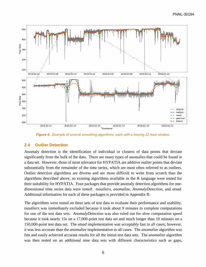
Figure 4 shows an example of several of the smoothing methods on flow rate data. Notice how
the moving mean (orange) is dramatically influenced by outliers and sudden changes. The
Gaussian (green) and LOWESS (red) smoothing both have smooth curves and no sharp corners
like median smoothing (blue). Although, the median smoothing tracks the center of the data even
through large discontinuities and near outliers.
PNNL-30194
6
Figure 4. Example of several smoothing algorithms, each with a moving 12-hour window.
2.4 Outlier Detection
Anomaly detection is the identification of individual or clusters of data points that deviate
significantly from the bulk of the data. There are many types of anomalies that could be found in
a data set. However, those of most relevance for HYPATIA are additive outlier points that deviate
substantially from the remainder of the time series, which are most often referred to as outliers.
Outlier detection algorithms are diverse and are more difficult to write from scratch than the
algorithms described above, so existing algorithms available in the R language were tested for
their suitability for HYPATIA. Four packages that provide anomaly detection algorithms for one-
dimensional time series data were tested: tsoutliers, anomalize, AnomalyDetection, and otsad.
Additional information for each of these packages is provided in Appendix B.
The algorithms were tested on three sets of test data to evaluate their performance and usability.
tsoutliers was immediately excluded because it took about 9 minutes to complete computations
for one of the test data sets. AnomalyDetection was also ruled out for slow computation speed
because it took nearly 15s on a 17,000-point test data set and much longer than 10 minutes on a
150,000-point test data set. The otsad implementation was acceptably fast in all cases; however,
it was less accurate than the anomalize implementation in all cases. The anomalize algorithm was
fast and easily achieved accurate results for all the initial test data sets. The anomalize algorithm
was then tested on an additional nine data sets with different characteristics such as gaps,

PNNL-30194
7
discontinuities, large size, periodicity, and more. It was determined that the algorithm performed
well on a wide range of input data but struggled when handling changes in variance and large
discontinuities.
The anomalize algorithm first uses Seasonal and Trend decomposition using Loess (STL) to split
the time series into seasonal, trend, and residual components. Because the HYPATIA data is not
seasonal, this portion of the decomposition does not provide much benefit. Removing the trend
component, though, is crucial and is achieved by locally estimated scatter plot smoothing
(LOESS). Once the trend is removed from the data, the interquartile range (IQR) of the remaining
residuals is used to define the outliers. The default setting is that any point with a residual three
times greater than the IQR of the residuals is classified as an outlier, but this factor can be adjusted.
The LOESS curve fitting and the IQR definition of the outlier for the residuals work well in most
cases. A specific drawback of the algorithm is that the LOESS curve fitting assumes a continuous
function and does not satisfactorily handle discontinuities in the time series. Additionally, because
the IQR is taken for all residuals in the entire time series, the band of inliers has constant width
and does not work well when the variance of the time series changes over time. These issues can
be seen in the data depicted in Figure 5.
Figure 5. Plot of results from outlier detection using the anomalize algorithm.
To remedy the deficiencies in the anomalize algorithm, a novel outlier detection algorithm was
written. The algorithm uses median smoothing with a sliding time window to remove the trend.
This method works well, even with outliers present and with discontinuities, but the size of the
sliding time window must be selected appropriately. By using a sliding median, the trend removal
is much more responsive to discontinuities in the series, while still robust to outliers. Once the
trend is removed, the inliers are defined within the sliding window. The upper bound on the inlier
range is proportional to the range between the 75th percentile and median of values within the time
window. Symmetrically, the lower bound on the inlier range is proportional to the range between
the 25th percentile and median of values within the time window. By defining the inlier range
based on the second and third quartile ranges, the algorithm responds well to changes in variance
within the series. The principle drawback is that this algorithm is currently much slower than the

PNNL-30194
8
anomalize algorithm. When tested on a HYPATIA flow sensor data set with ~28,000 data points,
it took about 30 seconds to compute. Figure 6 depicts the result of this revised algorithm on the
same set of data as shown in Figure 5.
Figure 6. Revised outlier detection with median smoothing and modified IQR inlier criteria.
2.5 Changepoint Detection
For changepoint detection, there are multiple types of changes to consider, including changes in
mean, in variance, in linear trend, in periodic frequency, in periodic amplitude, etc. The type of
changes most meaningful for HYPATIA are changes in mean and variance because there is no
significant seasonal or cyclical trend, and the data is characterized by rapid transitions between
states with (in most instances) no discernible trend between these states. Changes in mean and
variance for flow or pressure sensor data indicate changes in the state of P&T plant operations. A
sudden change in the variance of one sensor could also indicate a problem with measurements
from that sensor, perhaps indicating a need for maintenance.
Changepoint detection for both mean and variance is implemented with the changepoint package
for R (Killick and Eckley, 2014; Killick et al., 2016). The Pruned Exact Linear Time (PELT)
algorithm is used for detecting multiple changepoints. This algorithm iteratively checks the entire
data set for changes, then checks each partition until no more changes exceed the threshold defined
by the cost function (Killick et al., 2012). The coefficient on the cost function can be manually
specified by the user and is the primary means of tuning the algorithm’s sensitivity to changes.
The PELT algorithm is used for both detecting changes in mean and changes in variance. An
example of changepoint detection is depicted in Figure 7.

PNNL-30194
9
Figure 7. Example of changepoint detection, showing changes in the mean.
2.6 Mass Flow Rate Calculation
Mass flow rate is broadly defined to encompass both constituent mass and radionuclide activity.
The calculation for mass flow rate is simply flow rate multiplied by chemical concentration to
yield a quantity in either mass per time or activity per time, as shown in Equation 1.
𝑣𝑜𝑙𝑢𝑚𝑒
𝑡𝑖𝑚𝑒×
𝑚𝑎𝑠𝑠 𝑜𝑟 𝑎𝑐𝑡𝑖𝑣𝑖𝑡𝑦
𝑣𝑜𝑙𝑢𝑚𝑒=
𝑚𝑎𝑠𝑠 𝑜𝑟 𝑎𝑐𝑡𝑖𝑣𝑖𝑡𝑦
𝑡𝑖𝑚𝑒 (1)
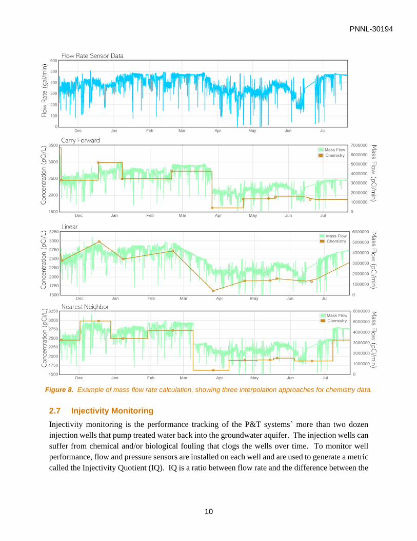
While the definition is simple, the difficulty lies in the disparate frequencies of sensor
measurements and chemistry data. Sensor measurements are available at a 15-minute frequency,
while chemistry data is generally collected at a monthly or quarterly frequency. A matching
approach was required to combine the chemistry and flow sensor information. Three approaches
were developed: carry forward, linear interpolation, and nearest-neighbor. The carry forward
approach takes the most recent known chemistry value and uses that value for all points afterward
until the next known chemistry value in time. The linear interpolation approach creates line
segments between all known chemistry values and uses the values of this linear estimation between
the known values. The nearest-neighbors approach uses the nearest known chemistry point
looking forward and backward in time. These three options are all reasonable strategies, so the
approach that is used for matching chemistry and sensor data is a matter of preference/engineering
judgement for the HYPATIA user. Figure 8 shows the flow rate sensor series (top panel) and the
three interpolation approaches for combing chemistry data (brown) and flow to obtain mass flow
rate (green).
PNNL-30194
10
Figure 8. Example of mass flow rate calculation, showing three interpolation approaches for chemistry data.
2.7 Injectivity Monitoring
Injectivity monitoring is the performance tracking of the P&T systems’ more than two dozen
injection wells that pump treated water back into the groundwater aquifer. The injection wells can
suffer from chemical and/or biological fouling that clogs the wells over time. To monitor well
performance, flow and pressure sensors are installed on each well and are used to generate a metric
called the Injectivity Quotient (IQ). IQ is a ratio between flow rate and the difference between the

PNNL-30194
11
dynamic water table measurement and the static water table, which is a measurement of injection
pressure (Equation 2).
𝐼𝑄 =𝑓𝑙𝑜𝑤 𝑟𝑎𝑡𝑒
𝑑𝑦𝑛𝑎𝑚𝑖𝑐 𝑤𝑎𝑡𝑒𝑟 𝑙𝑒𝑣𝑒𝑙 − 𝑠𝑡𝑎𝑡𝑖𝑐 𝑤𝑎𝑡𝑒𝑟 𝑙𝑒𝑣𝑒𝑙 ∝
𝑓𝑙𝑜𝑤 𝑟𝑎𝑡𝑒
𝑖𝑛𝑗𝑒𝑐𝑡𝑖𝑜𝑛 𝑝𝑟𝑒𝑠𝑠𝑢𝑟𝑒 (2)
Because flow rate and dynamic water level are both sensor measurements, they are noisy and
therefore cause large fluctuations in the IQ. While the IQ can illuminate some trends in injectivity,
they are often difficult to observe.
The Hall Plot method for injectivity monitoring is a possible alternative to the IQ that relies on
cumulatively integrating both the flow and pressure sensor data to smooth out noise and help reveal
long term trends. The horizontal axis of the Hall Plot is cumulative flow volume, while the vertical
axis is the running integral of pressure with time (units of pressure × time). Changes in the slope
of the Hall Plot then indicate changes in well injectivity.3 An increasing slope that bends upward
indicates a decline in injectivity because the ratio of pressure to flow is increasing. Conversely, a
slope that becomes less steep over time indicates an improvement in injectivity. The advantage of
the Hall Plot is that the resulting curve is smooth, making long-term changes in injectivity clearly
visible as deviations in the slope of the curve.
Figure 9 depicts an example of flow, pressure (injection well water level), IQ, and Hall Plot data.
3 “Applications for the Hall Plot Method for Monitoring and Prediction of PWRI Performance.” (website).
Advanatek International. http://www.advntk.com/pwrijip2003/pwri/final_reports/task_1/hall_plots/hall_plot_method_2.htm.

PNNL-30194
12
Figure 9. Example data for IQ and Hall Plot injectivity monitoring approaches.
2.8 Implementing R in AWS Lambda
AWS Lambda is a serverless platform for executing code in response to events such as HTTP
requests. Lambda has built-in support for Python and JavaScript, but not for the R language. Thus,
to host the outlier detection, changepoint algorithms, or any other R script, a method was required
for running R in Lambda. There are a few open source packages available that allow execution of
R code from a Python runtime environment. PypeR and rpy2 were both considered, but rpy2 had

PNNL-30194
13
too many required files and proved difficult to use. Therefore, PypeR (Xia, 2014) was adopted as
the chosen package.
When the R-base libraries are installed, there are many internal references to file locations, so it is
important to install R-base in the location where it will be used. This cannot be done within a
Lambda function, so a Docker container was used to simulate a Lambda environment. Docker is
a service that allows Windows to host Linux containers that can then simulate the Lambda
environment with the open source ‘docker-lambda’ container image. R-base and PypeR were
installed inside the simulated Lambda container and the files for both were then copied from the
Linux container to the Windows host machine. Once copied, file permissions were set to allow
execution of binary files. The copied files were zipped into a single file and uploaded to the AWS
Console. Once uploaded, the file was linked to a Lambda function as a layer. Execution of a
simple R code was conducted to verify that the layer files and R computational engine were
accessible and functioning properly.
3.0 Issues and Future Considerations
Not all of the functions developed in this work were given equal time or attention, and all could
be improved. The issues and suggested improvements to each function are detailed below.
3.1 Summing and Differencing
For the convenience of plotting, all millisecond timestamps are converted to Python DateTime
objects which are then used to align the input time series for addition or subtraction. The same
output could be achieved without this conversion and might improve the efficiency of the
algorithm.
3.2 Smoothing
The main deficiency in the smoothing algorithms are the computation speeds. For instance, the
Gaussian smoother takes about 10s on a time series with only ~5000 points. The slow step is likely
the indexing to create the sliding time window. This process does not need to be done sequentially,
so it is possible it could be parallelized. It might also be possible to perform this task without the
use of a “for” loop.
3.3 Outlier Detection
In the anomalize algorithm, the data is detrended using a LOESS smoothed curve and the inlier
range is proportional to the IQR of all the residuals. The LOESS smoothing method fails where
there are discontinuities in the trend, so the data near the edges of discontinuities are clipped. In
the revised outlier detection algorithm, this problem is avoided by using a running median, which
handles discontinuities well. The other issue with the anomalize algorithm was its inability to
handle changes in variance. The revised algorithm utilizes a sliding window approach and defines
the inlier range using the ranges of the second and third quartiles for setting the lower and upper
PNNL-30194
14
bounds, respectively. However, the revised algorithm is slow and takes 50-100 times longer than
the anomalize algorithm, so work is needed to improve its efficiency.
3.4 Changepoint Detection
The changepoint detection algorithm is very sensitive to outliers and readily detects them as
changes. It would be prudent to supply the user with information about this tendency, so they can
manually remove outliers before using changepoint detection. The changepoint algorithm itself
does not automatically remove outliers.
3.5 Mass Flow Rate Calculation
The mass flow rate calculation does not currently handle measurement units intelligently. The
only unit conversion applied is to convert from gallons to liters. Thus, volumetric flow rate,
reported in gallons per minute, and concentration, measured in quantity per liter, will cancel
appropriately and yield no volume units. It would be good to implement a logical algorithm that
converts/scales incoming measurements to a readable format for the number.
3.6 Injectivity Monitoring
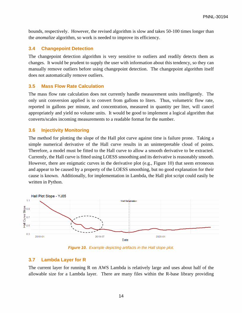
The method for plotting the slope of the Hall plot curve against time is failure prone. Taking a
simple numerical derivative of the Hall curve results in an uninterpretable cloud of points.
Therefore, a model must be fitted to the Hall curve to allow a smooth derivative to be extracted.
Currently, the Hall curve is fitted using LOESS smoothing and its derivative is reasonably smooth.
However, there are enigmatic curves in the derivative plot (e.g., Figure 10) that seem erroneous
and appear to be caused by a property of the LOESS smoothing, but no good explanation for their
cause is known. Additionally, for implementation in Lambda, the Hall plot script could easily be
written in Python.
Figure 10. Example depicting artifacts in the Hall slope plot.
3.7 Lambda Layer for R
The current layer for running R on AWS Lambda is relatively large and uses about half of the
allowable size for a Lambda layer. There are many files within the R-base library providing

PNNL-30194
15
functions that are not currently needed. If layer size becomes an issue, it would be helpful to
manually explore the R-base files and remove those that are not required.
4.0 Software Testing
The functions described in this report will be tested and reviewed in accordance with the Software
Quality Assurance Plan for the SOCRATES software (PNNL, 2020), which implements NQA-1
software quality. Testing of these analytic functions will encompass calculation tests, as well as
associated reviews of the data sources and testing of the HYPATIA interface functionality.
5.0 Summary
The objective of this study was to develop analytical algorithms to be implemented in HYPATIA,
a module of the SOCRATES tool suite aimed at supporting Hanford Site contractors and DOE
staff in the remediation of the Hanford Plateau. Historical operations at the Hanford Site resulted
in the contamination of groundwater at the 200 West Area with carbon tetrachloride and other
contaminants. As part of remediation efforts for the site, DOE constructed the 200 West Pump-
and-Treat System to contain and treat the contaminated groundwater. Within the P&T system,
sensors continuously monitor flow and pressure at many points, and chemistry data is sampled
intermittently throughout the plant. The Deep Vadose Zone Project at PNNL is developing the
HYPATIA module within the SOCRATES tool suite to provide access and analysis tools for the
P&T data. The HYPATIA module will benefit DOE staff and site contractors interested in
evaluating the data with respect to P&T plant treatment performance, optimization, or other
remedial decisions. Several functions were developed to provide data analytics functionality for
HYPATIA. These functions included summing, differencing, smoothing, outlier detection,
changepoint detection, mass flow rate calculation, and injectivity monitoring. These functions will
be incorporated for use in HYPATIA through deployment in AWS Lambda, for which a method
was developed to allow R code to execute within Lambda. Lambda already supports Python and
JavaScript. Thus, these functions can all be migrated to Lambda with only minor adjustments to
optimize their performance. Once in Lambda, the HYPATIA front end will provide the interface
for the user to call the functions on their data set of interest. However, the functions are not perfect
or complete and can be further improved.
6.0 References
Amazon Web Services. 2020. “boto3.” Available at: https://pypi.org/project/boto3/.
Chen, C., and L. Liu. 1993. “Forecasting Time Series with Outliers.” J. Forecasting, 12(1):13-
35. Available at: https://onlinelibrary.wiley.com/doi/abs/10.1002/for.3980120103.
Comprehensive Environmental Response, Compensation, and Liability Act. 1980. 42 U.S.C. §
9601-9675.

PNNL-30194
16
DOE. 2016. 200 West Pump and Treat Operations and Maintenance Plan. DOE/RL-2009-124,
Rev. 5, U.S. Department of Energy, Richland Operations Office, Richland, WA.
Available at: https://pdw.hanford.gov/document/0077130H.
DOE. 2020. “200 Area” (website). U.S. Department of Energy, Office of River Protection and
Richland Operations Office, Richland, WA. Available at:
https://www.hanford.gov/page.cfm/200Area.
Hart, M. 2020. “docker-lambda.” Available at: https://github.com/lambci/docker-lambda.
Jones, M.C., S.J. Davies, and B.U. Park. 1994. “Versions of Kernel-type Regression
Estimators.” J. Am. Stat. Assn., 89(427):825-832.
Killick, R., P. Fearnhead, I.A. Eckley. 2012. “Optimal Detection of Changepoints with a
Linear.” arXiv:1101.1438v3. Available at: https://arxiv.org/pdf/1101.1438.pdf.
Killick, R., and I.A. Eckley. 2014. “changepoint: An R Package for Changepoint Analysis.”
J. Statistical Software, 58(3):1-19. Available at: http://www.jstatsoft.org/v58/i03/.
Killick, R., K. Haynes, I.A. Eckley. 2016. “changepoint: An R package for Changepoint
Analysis.” R package version 2.2.2. Available at: https://CRAN.R-
project.org/package=changepoint.
Perktold, J., S. Seabold, and J. Taylor. 2020. “statsmodels.” Available at:
https://www.statsmodels.org/stable/index.html.
PNNL. 2018. “SOCRATES Extracts Wisdom from Groundwater Data.” Pacific Northwest
National Laboratory, Richland WA. Available at: https://www.pnnl.gov/news-
media/socrates-extracts-wisdom-groundwater-data.
PNNL. 2020. Software Quality Assurance Plan: SOCRATES. DVZ-SQAP-003, Rev. 3, Pacific
Northwest National Laboratory, Richland WA.
Raza, H., G. Prasad, and Y. Li. 2015. “EWMA Model Based Shift Detection Methods for
Detecting Covariate Shifts in Non-stationary Environments.” Pattern Recognition,
48(3):659-669. Available at:
https://www.sciencedirect.com/science/article/abs/pii/S0031320314002878.
WDOE, EPA, DOE. 1989 (as amended through 2020). “Hanford Federal Facility Agreement
and Consent Order.” U.S. Department of Energy, Office of River Protection and
Richland Operations Office, Richland, WA. Available at:
https://www.hanford.gov/files.cfm/HFFACO.pdf.
Xia, X. 2014. “PypeR.” Available at: https://pypi.org/project/PypeR/.
PNNL-30194
A.1
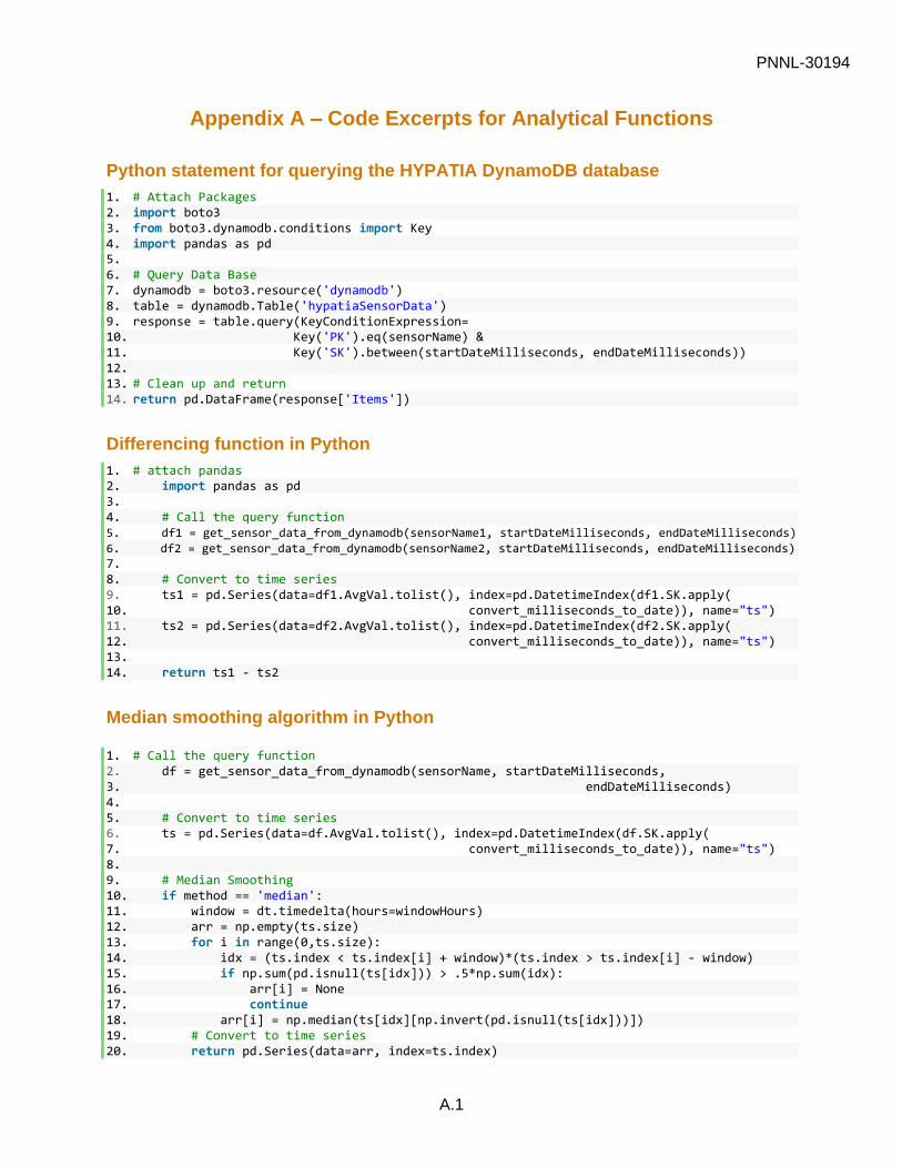
Appendix A – Code Excerpts for Analytical Functions
Python statement for querying the HYPATIA DynamoDB database
1. # Attach Packages 2. import boto3 3. from boto3.dynamodb.conditions import Key 4. import pandas as pd 5. 6. # Query Data Base 7. dynamodb = boto3.resource('dynamodb') 8. table = dynamodb.Table('hypatiaSensorData') 9. response = table.query(KeyConditionExpression= 10. Key('PK').eq(sensorName) & 11. Key('SK').between(startDateMilliseconds, endDateMilliseconds)) 12. 13. # Clean up and return 14. return pd.DataFrame(response['Items'])
Differencing function in Python
1. # attach pandas 2. import pandas as pd 3. 4. # Call the query function 5. df1 = get_sensor_data_from_dynamodb(sensorName1, startDateMilliseconds, endDateMilliseconds) 6. df2 = get_sensor_data_from_dynamodb(sensorName2, startDateMilliseconds, endDateMilliseconds) 7. 8. # Convert to time series 9. ts1 = pd.Series(data=df1.AvgVal.tolist(), index=pd.DatetimeIndex(df1.SK.apply( 10. convert_milliseconds_to_date)), name="ts") 11. ts2 = pd.Series(data=df2.AvgVal.tolist(), index=pd.DatetimeIndex(df2.SK.apply( 12. convert_milliseconds_to_date)), name="ts") 13. 14. return ts1 - ts2
Median smoothing algorithm in Python
1. # Call the query function 2. df = get_sensor_data_from_dynamodb(sensorName, startDateMilliseconds, 3. endDateMilliseconds) 4. 5. # Convert to time series 6. ts = pd.Series(data=df.AvgVal.tolist(), index=pd.DatetimeIndex(df.SK.apply( 7. convert_milliseconds_to_date)), name="ts") 8. 9. # Median Smoothing 10. if method == 'median': 11. window = dt.timedelta(hours=windowHours) 12. arr = np.empty(ts.size) 13. for i in range(0,ts.size): 14. idx = (ts.index < ts.index[i] + window)*(ts.index > ts.index[i] - window) 15. if np.sum(pd.isnull(ts[idx])) > .5*np.sum(idx): 16. arr[i] = None 17. continue 18. arr[i] = np.median(ts[idx][np.invert(pd.isnull(ts[idx]))]) 19. # Convert to time series 20. return pd.Series(data=arr, index=ts.index)
PNNL-30194
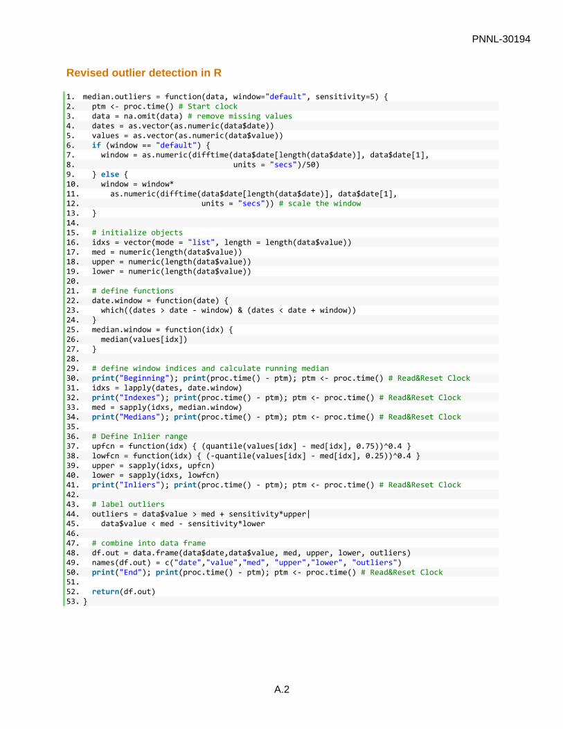
A.2
Revised outlier detection in R
1. median.outliers = function(data, window="default", sensitivity=5) { 2. ptm <- proc.time() # Start clock 3. data = na.omit(data) # remove missing values 4. dates = as.vector(as.numeric(data$date)) 5. values = as.vector(as.numeric(data$value)) 6. if (window == "default") { 7. window = as.numeric(difftime(data$date[length(data$date)], data$date[1], 8. units = "secs")/50) 9. } else { 10. window = window* 11. as.numeric(difftime(data$date[length(data$date)], data$date[1], 12. units = "secs")) # scale the window 13. } 14. 15. # initialize objects 16. idxs = vector(mode = "list", length = length(data$value)) 17. med = numeric(length(data$value)) 18. upper = numeric(length(data$value)) 19. lower = numeric(length(data$value)) 20. 21. # define functions 22. date.window = function(date) { 23. which((dates > date - window) & (dates < date + window)) 24. } 25. median.window = function(idx) { 26. median(values[idx]) 27. } 28. 29. # define window indices and calculate running median 30. print("Beginning"); print(proc.time() - ptm); ptm <- proc.time() # Read&Reset Clock 31. idxs = lapply(dates, date.window) 32. print("Indexes"); print(proc.time() - ptm); ptm <- proc.time() # Read&Reset Clock 33. med = sapply(idxs, median.window) 34. print("Medians"); print(proc.time() - ptm); ptm <- proc.time() # Read&Reset Clock 35. 36. # Define Inlier range 37. upfcn = function(idx) { (quantile(values[idx] - med[idx], 0.75))^0.4 } 38. lowfcn = function(idx) { (-quantile(values[idx] - med[idx], 0.25))^0.4 } 39. upper = sapply(idxs, upfcn) 40. lower = sapply(idxs, lowfcn) 41. print("Inliers"); print(proc.time() - ptm); ptm <- proc.time() # Read&Reset Clock 42. 43. # label outliers 44. outliers = data$value > med + sensitivity*upper| 45. data$value < med - sensitivity*lower 46. 47. # combine into data frame 48. df.out = data.frame(data$date,data$value, med, upper, lower, outliers) 49. names(df.out) = c("date","value","med", "upper","lower", "outliers") 50. print("End"); print(proc.time() - ptm); ptm <- proc.time() # Read&Reset Clock 51. 52. return(df.out) 53. }

PNNL-30194
A.3
Linear interpolation for chemistry data in mass flow rate calculation in JavaScript
1. function massFlowCalcLin(data) { 2. // Calculate Mass Flow with Linear interpolation 3. 4. // variable declaration 5. let massFlow = []; 6. let interpData = []; 7. let concLog = []; 8. let currentConc = 0; 9. let mass; 10. let idx = 0; 11. 12. // Use linear interpolation to determine the current concentration 13. for (i=0; i<data.flowData.length; i++) { 14. flowDate = data.flowData[i][0]; 15. // iterate through the dates on the flow date until within the correct time range 16. if (flowDate >= data.startDate && flowDate <= data.endDate) { 17. if (flowDate >= data.concData[idx][0]) { 18. // Increase the date on the concentration data until it exceeds the flow date 19. while (flowDate >= data.concData[idx][0]) { 20. idx++; 21. } 22. } 23. // Calculate the concentration using a line 24. slope = (data.concData[idx][1]-data.concData[idx- 25. 1][1])/(data.concData[idx][0]-data.concData[idx-1][0]); 26. currentConc = slope*(flowDate-data.concData[idx-1][0]) + 27. data.concData[idx-1][1]; 28. concLog.push(currentConc) 29. interpData.push([flowDate, currentConc]) 30. // Unit conversion from gallons to liters here 31. mass = currentConc*data.flowData[i][1]*3.785; 32. massFlow.push([flowDate, mass]); 33. } 34. }; 35. }
Flow rate and pressure integration for Hall plot analysis in R
1. # integrate the flow data 2. plotdf$fsum[1] = 0 3. for (i in 2:length(plotdf$time)) { 4. plotdf$fsum[i] = plotdf$fsum[i-1] + 0.5*(plotdf$flowA[i]+ 5. plotdf$flowA[i-1])*(plotdf$time[i]-plotdf$time[i-1]) 6. } 7. # Integrate the pressure data 8. plotdf$psum[1] = 0 9. for (i in 2:length(plotdf$time)) { 10. plotdf$psum[i] = plotdf$psum[i-1] + 0.5*(plotdf$head[i]+ 11. plotdf$head[i-1])*(plotdf$time[i]-plotdf$time[i-1]) 12. }

PNNL-30194
B.1
Appendix B – Outlier Detection Algorithms
B.1 tso from tsoutliers
Implements the procedure described in Chen and Liu (1993) for automatically detecting
innovational outliers, additive outliers, level shifts, temporary changes, and seasonal level shifts.
B.2 anomalize from anomalize
A ‘tidy’ implementation of methods from the forecast and AnomalyDetection packages. Tidy is a
workflow style utilizing pipes to link functions together. This algorithm allows for time
decomposition via seasonal decomposition of time series by loess and seasonal decomposition by
piecewise medians. It also allows for anomaly detection of residuals by either inner quartile range
or generalized studentized deviation. There are four combinations for matching these methods in
addition to adjustable parameters.
B.3 AnomalyDetectionTs from AnomalyDetection
This package is developed by twitter and employs trend decomposition with piecewise median
approximation. Outliers are then detected from the decomposition residual using the Generalized
Extreme Studentized Deviation test. The anomalize algorithm can implement this same algorithm
with a faster computational speed.
B.4 OcpSdEwma from otsad
This function calculates anomalies with the Shift Detection – Exponentially Weighted Moving
Average (SD-EWMA) algorithm. The method is derived from Raza et al. (2015).

Pacific Northwest National Laboratory
902 Battelle Boulevard
P.O. Box 999
Richland, WA 99354
1-888-375-PNNL (7665)
www.pnnl.gov