analytical heat transfer
TRANSCRIPT
ANALYTICAL HEAT TRANSFER
Mihir Sen
Department of Aerospace and Mechanical Engineering
University of Notre Dame
Notre Dame, IN 46556
May 6, 2008
Preface
These are lecture notes for AME60634: Intermediate Heat Transfer, a second course on heat transferfor undergraduate seniors and beginning graduate students. At this stage the student can begin toapply knowledge of mathematics and computational methods to the problems of heat transfer.Thus, in addition to some undergraduate knowledge of heat transfer, students taking this course areexpected to be familiar with vector algebra, linear algebra, ordinary differential equations, particleand rigid-body dynamics, thermodynamics, and integral and differential analysis in fluid mechanics.The use of computers is essential both for the purpose of computation as well as for display andvisualization of results.
At present these notes are in the process of being written; the student is encouraged to makeextensive use of the literature listed in the bibliography. The students are also expected to attemptthe problems at the end of each chapter to reinforce their learning.
I will be glad to receive comments on these notes, and have mistakes brought to my attention.
Mihir SenDepartment of Aerospace and Mechanical Engineering
University of Notre Dame
Copyright c© by M. Sen, 2008
i
Contents
Preface i
I Review 1
1 Introductory heat transfer 2
1.1 Fundamentals . . . . . . . . . . . . . . . . . . . . . . . . . . . . . . . . . . . . . . . . 21.1.1 Definitions . . . . . . . . . . . . . . . . . . . . . . . . . . . . . . . . . . . . . 21.1.2 Energy balance . . . . . . . . . . . . . . . . . . . . . . . . . . . . . . . . . . . 21.1.3 States of matter . . . . . . . . . . . . . . . . . . . . . . . . . . . . . . . . . . 3
1.2 Conduction . . . . . . . . . . . . . . . . . . . . . . . . . . . . . . . . . . . . . . . . . 31.2.1 Governing equation . . . . . . . . . . . . . . . . . . . . . . . . . . . . . . . . 31.2.2 Fins . . . . . . . . . . . . . . . . . . . . . . . . . . . . . . . . . . . . . . . . . 31.2.3 Separation of variables . . . . . . . . . . . . . . . . . . . . . . . . . . . . . . . 51.2.4 Similarity variable . . . . . . . . . . . . . . . . . . . . . . . . . . . . . . . . . 51.2.5 Lumped-parameter approximation . . . . . . . . . . . . . . . . . . . . . . . . 5
1.3 Convection . . . . . . . . . . . . . . . . . . . . . . . . . . . . . . . . . . . . . . . . . 71.3.1 Governing equations . . . . . . . . . . . . . . . . . . . . . . . . . . . . . . . . 81.3.2 Flat-plate boundary-layer theory . . . . . . . . . . . . . . . . . . . . . . . . . 81.3.3 Heat transfer coefficients . . . . . . . . . . . . . . . . . . . . . . . . . . . . . . 8
1.4 Radiation . . . . . . . . . . . . . . . . . . . . . . . . . . . . . . . . . . . . . . . . . . 91.4.1 Electromagnetic radiation . . . . . . . . . . . . . . . . . . . . . . . . . . . . . 91.4.2 View factors . . . . . . . . . . . . . . . . . . . . . . . . . . . . . . . . . . . . 11
1.5 Boiling and condensation . . . . . . . . . . . . . . . . . . . . . . . . . . . . . . . . . 111.5.1 Boiling curve . . . . . . . . . . . . . . . . . . . . . . . . . . . . . . . . . . . . 111.5.2 Critical heat flux . . . . . . . . . . . . . . . . . . . . . . . . . . . . . . . . . . 111.5.3 Film boiling . . . . . . . . . . . . . . . . . . . . . . . . . . . . . . . . . . . . . 111.5.4 Condensation . . . . . . . . . . . . . . . . . . . . . . . . . . . . . . . . . . . . 11
1.6 Heat exchangers . . . . . . . . . . . . . . . . . . . . . . . . . . . . . . . . . . . . . . 111.6.1 Parallel- and counter-flow . . . . . . . . . . . . . . . . . . . . . . . . . . . . . 131.6.2 HX relations . . . . . . . . . . . . . . . . . . . . . . . . . . . . . . . . . . . . 141.6.3 Design methodology . . . . . . . . . . . . . . . . . . . . . . . . . . . . . . . . 151.6.4 Correlations . . . . . . . . . . . . . . . . . . . . . . . . . . . . . . . . . . . . . 151.6.5 Extended surfaces . . . . . . . . . . . . . . . . . . . . . . . . . . . . . . . . . 15
Problems . . . . . . . . . . . . . . . . . . . . . . . . . . . . . . . . . . . . . . . . . . . . . 15
ii
CONTENTS iii
II No spatial dimension 17
2 Dynamics 18
2.1 Variable heat transfer coefficient . . . . . . . . . . . . . . . . . . . . . . . . . . . . . 182.1.1 Radiative cooling . . . . . . . . . . . . . . . . . . . . . . . . . . . . . . . . . . 192.1.2 Convective with weak radiation . . . . . . . . . . . . . . . . . . . . . . . . . . 20
2.2 Radiation in an enclosure . . . . . . . . . . . . . . . . . . . . . . . . . . . . . . . . . 212.3 Long time behavior . . . . . . . . . . . . . . . . . . . . . . . . . . . . . . . . . . . . . 21
2.3.1 Linear analysis . . . . . . . . . . . . . . . . . . . . . . . . . . . . . . . . . . . 212.3.2 Nonlinear analysis . . . . . . . . . . . . . . . . . . . . . . . . . . . . . . . . . 22
2.4 Time-dependent T∞ . . . . . . . . . . . . . . . . . . . . . . . . . . . . . . . . . . . . 222.4.1 Linear . . . . . . . . . . . . . . . . . . . . . . . . . . . . . . . . . . . . . . . . 222.4.2 Oscillatory . . . . . . . . . . . . . . . . . . . . . . . . . . . . . . . . . . . . . 23
2.5 Two-fluid problem . . . . . . . . . . . . . . . . . . . . . . . . . . . . . . . . . . . . . 242.6 Two-body problem . . . . . . . . . . . . . . . . . . . . . . . . . . . . . . . . . . . . . 25
2.6.1 Convective . . . . . . . . . . . . . . . . . . . . . . . . . . . . . . . . . . . . . 252.6.2 Radiative . . . . . . . . . . . . . . . . . . . . . . . . . . . . . . . . . . . . . . 26
Problems . . . . . . . . . . . . . . . . . . . . . . . . . . . . . . . . . . . . . . . . . . . . . 26
3 Control 27
3.1 Introduction . . . . . . . . . . . . . . . . . . . . . . . . . . . . . . . . . . . . . . . . . 273.2 Systems . . . . . . . . . . . . . . . . . . . . . . . . . . . . . . . . . . . . . . . . . . . 28
3.2.1 Systems without control . . . . . . . . . . . . . . . . . . . . . . . . . . . . . . 283.2.2 Systems with control . . . . . . . . . . . . . . . . . . . . . . . . . . . . . . . 29
3.3 Linear systems theory . . . . . . . . . . . . . . . . . . . . . . . . . . . . . . . . . . . 293.3.1 Ordinary differential equations . . . . . . . . . . . . . . . . . . . . . . . . . . 303.3.2 Algebraic-differential equations . . . . . . . . . . . . . . . . . . . . . . . . . . 31
3.4 Nonlinear aspects . . . . . . . . . . . . . . . . . . . . . . . . . . . . . . . . . . . . . . 313.4.1 Models . . . . . . . . . . . . . . . . . . . . . . . . . . . . . . . . . . . . . . . 313.4.2 Controllability and reachability . . . . . . . . . . . . . . . . . . . . . . . . . . 313.4.3 Bounded variables . . . . . . . . . . . . . . . . . . . . . . . . . . . . . . . . . 313.4.4 Relay and hysteresis . . . . . . . . . . . . . . . . . . . . . . . . . . . . . . . . 32
3.5 System identification . . . . . . . . . . . . . . . . . . . . . . . . . . . . . . . . . . . . 323.6 Control strategies . . . . . . . . . . . . . . . . . . . . . . . . . . . . . . . . . . . . . 33
3.6.1 Mathematical model . . . . . . . . . . . . . . . . . . . . . . . . . . . . . . . . 333.6.2 On-off control . . . . . . . . . . . . . . . . . . . . . . . . . . . . . . . . . . . . 333.6.3 PID control . . . . . . . . . . . . . . . . . . . . . . . . . . . . . . . . . . . . . 34
Problems . . . . . . . . . . . . . . . . . . . . . . . . . . . . . . . . . . . . . . . . . . . . . 35
III One spatial dimension 37
4 Conduction 38
4.1 Structures . . . . . . . . . . . . . . . . . . . . . . . . . . . . . . . . . . . . . . . . . . 384.2 Fin theory . . . . . . . . . . . . . . . . . . . . . . . . . . . . . . . . . . . . . . . . . . 38
4.2.1 Long time solution . . . . . . . . . . . . . . . . . . . . . . . . . . . . . . . . . 384.2.2 Shape optimization of convective fin . . . . . . . . . . . . . . . . . . . . . . . 39
4.3 Fin structure . . . . . . . . . . . . . . . . . . . . . . . . . . . . . . . . . . . . . . . . 41
CONTENTS iv
4.4 Fin with convection and radiation . . . . . . . . . . . . . . . . . . . . . . . . . . . . 414.4.1 Annular fin . . . . . . . . . . . . . . . . . . . . . . . . . . . . . . . . . . . . . 43
4.5 Perturbations of one-dimensional conduction . . . . . . . . . . . . . . . . . . . . . . 434.5.1 Temperature-dependent conductivity . . . . . . . . . . . . . . . . . . . . . . . 434.5.2 Eccentric annulus . . . . . . . . . . . . . . . . . . . . . . . . . . . . . . . . . . 44
4.6 Transient conduction . . . . . . . . . . . . . . . . . . . . . . . . . . . . . . . . . . . . 464.7 Linear diffusion . . . . . . . . . . . . . . . . . . . . . . . . . . . . . . . . . . . . . . . 474.8 Nonlinear diffusion . . . . . . . . . . . . . . . . . . . . . . . . . . . . . . . . . . . . . 484.9 Stability by energy method . . . . . . . . . . . . . . . . . . . . . . . . . . . . . . . . 51
4.9.1 Linear . . . . . . . . . . . . . . . . . . . . . . . . . . . . . . . . . . . . . . . . 514.9.2 Nonlinear . . . . . . . . . . . . . . . . . . . . . . . . . . . . . . . . . . . . . . 51
4.10 Self-similar structures . . . . . . . . . . . . . . . . . . . . . . . . . . . . . . . . . . . 524.11 Non-Cartesian coordinates . . . . . . . . . . . . . . . . . . . . . . . . . . . . . . . . . 524.12 Thermal control . . . . . . . . . . . . . . . . . . . . . . . . . . . . . . . . . . . . . . 534.13 Multiple scales . . . . . . . . . . . . . . . . . . . . . . . . . . . . . . . . . . . . . . . 55Problems . . . . . . . . . . . . . . . . . . . . . . . . . . . . . . . . . . . . . . . . . . . . . 55
5 Forced convection 57
5.1 Hydrodynamics . . . . . . . . . . . . . . . . . . . . . . . . . . . . . . . . . . . . . . . 575.1.1 Mass conservation . . . . . . . . . . . . . . . . . . . . . . . . . . . . . . . . . 575.1.2 Momentum equation . . . . . . . . . . . . . . . . . . . . . . . . . . . . . . . . 575.1.3 Long time behavior . . . . . . . . . . . . . . . . . . . . . . . . . . . . . . . . . 59
5.2 Energy equation . . . . . . . . . . . . . . . . . . . . . . . . . . . . . . . . . . . . . . 605.2.1 Known heat rate . . . . . . . . . . . . . . . . . . . . . . . . . . . . . . . . . . 615.2.2 Convection with known outside temperature . . . . . . . . . . . . . . . . . . 62
5.3 Single duct . . . . . . . . . . . . . . . . . . . . . . . . . . . . . . . . . . . . . . . . . 625.3.1 Steady state . . . . . . . . . . . . . . . . . . . . . . . . . . . . . . . . . . . . . 635.3.2 Unsteady dynamics . . . . . . . . . . . . . . . . . . . . . . . . . . . . . . . . . 645.3.3 Perfectly insulated duct . . . . . . . . . . . . . . . . . . . . . . . . . . . . . . 645.3.4 Constant ambient temperature . . . . . . . . . . . . . . . . . . . . . . . . . . 645.3.5 Periodic inlet and ambient temperature . . . . . . . . . . . . . . . . . . . . . 655.3.6 Effect of wall . . . . . . . . . . . . . . . . . . . . . . . . . . . . . . . . . . . . 65
5.4 Two-fluid configuration . . . . . . . . . . . . . . . . . . . . . . . . . . . . . . . . . . 665.5 Flow between plates with viscous dissipation . . . . . . . . . . . . . . . . . . . . . . 675.6 Regenerator . . . . . . . . . . . . . . . . . . . . . . . . . . . . . . . . . . . . . . . . . 685.7 Radial flow between disks . . . . . . . . . . . . . . . . . . . . . . . . . . . . . . . . . 695.8 Networks . . . . . . . . . . . . . . . . . . . . . . . . . . . . . . . . . . . . . . . . . . 69
5.8.1 Hydrodynamics . . . . . . . . . . . . . . . . . . . . . . . . . . . . . . . . . . . 705.8.2 Thermal networks . . . . . . . . . . . . . . . . . . . . . . . . . . . . . . . . . 73
5.9 Thermal control . . . . . . . . . . . . . . . . . . . . . . . . . . . . . . . . . . . . . . 735.9.1 Control with heat transfer coefficient . . . . . . . . . . . . . . . . . . . . . . . 735.9.2 Multiple room temperatures . . . . . . . . . . . . . . . . . . . . . . . . . . . . 735.9.3 Two rooms . . . . . . . . . . . . . . . . . . . . . . . . . . . . . . . . . . . . . 745.9.4 Temperature in long duct . . . . . . . . . . . . . . . . . . . . . . . . . . . . . 74
Problems . . . . . . . . . . . . . . . . . . . . . . . . . . . . . . . . . . . . . . . . . . . . . 76
CONTENTS v
6 Natural convection 78
6.1 Modeling . . . . . . . . . . . . . . . . . . . . . . . . . . . . . . . . . . . . . . . . . . 786.1.1 Mass conservation . . . . . . . . . . . . . . . . . . . . . . . . . . . . . . . . . 786.1.2 Momentum equation . . . . . . . . . . . . . . . . . . . . . . . . . . . . . . . . 796.1.3 Energy equation . . . . . . . . . . . . . . . . . . . . . . . . . . . . . . . . . . 80
6.2 Known heat rate . . . . . . . . . . . . . . . . . . . . . . . . . . . . . . . . . . . . . . 816.2.1 Steady state, no axial conduction . . . . . . . . . . . . . . . . . . . . . . . . . 816.2.2 Axial conduction effects . . . . . . . . . . . . . . . . . . . . . . . . . . . . . . 856.2.3 Toroidal geometry . . . . . . . . . . . . . . . . . . . . . . . . . . . . . . . . . 886.2.4 Dynamic analysis . . . . . . . . . . . . . . . . . . . . . . . . . . . . . . . . . . 936.2.5 Nonlinear analysis . . . . . . . . . . . . . . . . . . . . . . . . . . . . . . . . . 101
6.3 Known wall temperature . . . . . . . . . . . . . . . . . . . . . . . . . . . . . . . . . . 1066.4 Mixed condition . . . . . . . . . . . . . . . . . . . . . . . . . . . . . . . . . . . . . . 107
6.4.1 Modeling . . . . . . . . . . . . . . . . . . . . . . . . . . . . . . . . . . . . . . 1086.4.2 Steady State . . . . . . . . . . . . . . . . . . . . . . . . . . . . . . . . . . . . 1096.4.3 Dynamic Analysis . . . . . . . . . . . . . . . . . . . . . . . . . . . . . . . . . 1126.4.4 Nonlinear analysis . . . . . . . . . . . . . . . . . . . . . . . . . . . . . . . . . 116
6.5 Perturbation of one-dimensional flow . . . . . . . . . . . . . . . . . . . . . . . . . . . 1196.6 Thermal control . . . . . . . . . . . . . . . . . . . . . . . . . . . . . . . . . . . . . . 119Problems . . . . . . . . . . . . . . . . . . . . . . . . . . . . . . . . . . . . . . . . . . . . . 119
7 Moving boundary 123
7.1 Stefan problems . . . . . . . . . . . . . . . . . . . . . . . . . . . . . . . . . . . . . . . 1237.1.1 Neumann’s solution . . . . . . . . . . . . . . . . . . . . . . . . . . . . . . . . 1237.1.2 Goodman’s integral . . . . . . . . . . . . . . . . . . . . . . . . . . . . . . . . 124
IV Multiple spatial dimensions 125
8 Conduction 126
8.1 Steady-state problems . . . . . . . . . . . . . . . . . . . . . . . . . . . . . . . . . . . 1268.2 Transient problems . . . . . . . . . . . . . . . . . . . . . . . . . . . . . . . . . . . . . 126
8.2.1 Two-dimensional fin . . . . . . . . . . . . . . . . . . . . . . . . . . . . . . . . 1268.3 Radiating fins . . . . . . . . . . . . . . . . . . . . . . . . . . . . . . . . . . . . . . . . 1278.4 Non-Cartesian coordinates . . . . . . . . . . . . . . . . . . . . . . . . . . . . . . . . . 127Problems . . . . . . . . . . . . . . . . . . . . . . . . . . . . . . . . . . . . . . . . . . . . . 127
9 Forced convection 128
9.1 Low Reynolds numbers . . . . . . . . . . . . . . . . . . . . . . . . . . . . . . . . . . . 1289.2 Potential flow . . . . . . . . . . . . . . . . . . . . . . . . . . . . . . . . . . . . . . . . 128
9.2.1 Two-dimensional flow . . . . . . . . . . . . . . . . . . . . . . . . . . . . . . . 1289.3 Leveque’s solution . . . . . . . . . . . . . . . . . . . . . . . . . . . . . . . . . . . . . 1289.4 Multiple solutions . . . . . . . . . . . . . . . . . . . . . . . . . . . . . . . . . . . . . 1289.5 Plate heat exchangers . . . . . . . . . . . . . . . . . . . . . . . . . . . . . . . . . . . 1289.6 Falkner-Skan boundary flows . . . . . . . . . . . . . . . . . . . . . . . . . . . . . . . 132Problems . . . . . . . . . . . . . . . . . . . . . . . . . . . . . . . . . . . . . . . . . . . . . 132
CONTENTS vi
10 Natural convection 133
10.1 Governing equations . . . . . . . . . . . . . . . . . . . . . . . . . . . . . . . . . . . . 13310.2 Cavities . . . . . . . . . . . . . . . . . . . . . . . . . . . . . . . . . . . . . . . . . . . 13310.3 Marangoni convection . . . . . . . . . . . . . . . . . . . . . . . . . . . . . . . . . . . 133Problems . . . . . . . . . . . . . . . . . . . . . . . . . . . . . . . . . . . . . . . . . . . . . 133
11 Porous media 134
11.1 Governing equations . . . . . . . . . . . . . . . . . . . . . . . . . . . . . . . . . . . . 13411.1.1 Darcy’s equation . . . . . . . . . . . . . . . . . . . . . . . . . . . . . . . . . . 13411.1.2 Forchheimer’s equation . . . . . . . . . . . . . . . . . . . . . . . . . . . . . . 13411.1.3 Brinkman’s equation . . . . . . . . . . . . . . . . . . . . . . . . . . . . . . . . 13511.1.4 Energy equation . . . . . . . . . . . . . . . . . . . . . . . . . . . . . . . . . . 135
11.2 Forced convection . . . . . . . . . . . . . . . . . . . . . . . . . . . . . . . . . . . . . . 13511.2.1 Plane wall at constant temperature . . . . . . . . . . . . . . . . . . . . . . . . 13511.2.2 Stagnation-point flow . . . . . . . . . . . . . . . . . . . . . . . . . . . . . . . 13711.2.3 Thermal wakes . . . . . . . . . . . . . . . . . . . . . . . . . . . . . . . . . . . 138
11.3 Natural convection . . . . . . . . . . . . . . . . . . . . . . . . . . . . . . . . . . . . . 13911.3.1 Linear stability . . . . . . . . . . . . . . . . . . . . . . . . . . . . . . . . . . . 13911.3.2 Steady-state inclined layer solutions . . . . . . . . . . . . . . . . . . . . . . . 142
Problems . . . . . . . . . . . . . . . . . . . . . . . . . . . . . . . . . . . . . . . . . . . . . 147
12 Moving boundary 148
12.1 Stefan problems . . . . . . . . . . . . . . . . . . . . . . . . . . . . . . . . . . . . . . . 148
V Complex systems 149
13 Radiation 150
13.1 Monte Carlo methods . . . . . . . . . . . . . . . . . . . . . . . . . . . . . . . . . . . 150Problems . . . . . . . . . . . . . . . . . . . . . . . . . . . . . . . . . . . . . . . . . . . . . 150
14 Boiling and condensation 151
14.1 Homogeneous nucleation . . . . . . . . . . . . . . . . . . . . . . . . . . . . . . . . . . 151
15 Microscale heat transfer 152
15.1 Diffusion by random walk . . . . . . . . . . . . . . . . . . . . . . . . . . . . . . . . . 15215.1.1 One-dimensional . . . . . . . . . . . . . . . . . . . . . . . . . . . . . . . . . . 15215.1.2 Multi-dimensional . . . . . . . . . . . . . . . . . . . . . . . . . . . . . . . . . 153
15.2 Boltzmann transport equation . . . . . . . . . . . . . . . . . . . . . . . . . . . . . . . 15315.2.1 Relaxation-time approximation . . . . . . . . . . . . . . . . . . . . . . . . . . 153
15.3 Phonons . . . . . . . . . . . . . . . . . . . . . . . . . . . . . . . . . . . . . . . . . . . 15415.3.1 Single atom type . . . . . . . . . . . . . . . . . . . . . . . . . . . . . . . . . . 15415.3.2 Two atom types . . . . . . . . . . . . . . . . . . . . . . . . . . . . . . . . . . 155
15.4 Thin films . . . . . . . . . . . . . . . . . . . . . . . . . . . . . . . . . . . . . . . . . . 156
16 Bioheat transfer 157
16.1 Mathematical models . . . . . . . . . . . . . . . . . . . . . . . . . . . . . . . . . . . . 157
CONTENTS vii
17 Heat exchangers 158
17.1 Fin analysis . . . . . . . . . . . . . . . . . . . . . . . . . . . . . . . . . . . . . . . . . 15817.2 Porous medium analogy . . . . . . . . . . . . . . . . . . . . . . . . . . . . . . . . . . 15817.3 Heat transfer augmentation . . . . . . . . . . . . . . . . . . . . . . . . . . . . . . . . 15817.4 Maldistribution effects . . . . . . . . . . . . . . . . . . . . . . . . . . . . . . . . . . . 15817.5 Microchannel heat exchangers . . . . . . . . . . . . . . . . . . . . . . . . . . . . . . . 15817.6 Radiation effects . . . . . . . . . . . . . . . . . . . . . . . . . . . . . . . . . . . . . . 15817.7 Transient behavior . . . . . . . . . . . . . . . . . . . . . . . . . . . . . . . . . . . . . 15817.8 Correlations . . . . . . . . . . . . . . . . . . . . . . . . . . . . . . . . . . . . . . . . . 159
17.8.1 Least squares method . . . . . . . . . . . . . . . . . . . . . . . . . . . . . . . 15917.9 Compressible flow . . . . . . . . . . . . . . . . . . . . . . . . . . . . . . . . . . . . . 15917.10Thermal control . . . . . . . . . . . . . . . . . . . . . . . . . . . . . . . . . . . . . . 15917.11Control of complex thermal systems . . . . . . . . . . . . . . . . . . . . . . . . . . . 161
17.11.1Hydronic networks . . . . . . . . . . . . . . . . . . . . . . . . . . . . . . . . . 16117.11.2Other applications . . . . . . . . . . . . . . . . . . . . . . . . . . . . . . . . . 162
17.12Conclusions . . . . . . . . . . . . . . . . . . . . . . . . . . . . . . . . . . . . . . . . . 165Problems . . . . . . . . . . . . . . . . . . . . . . . . . . . . . . . . . . . . . . . . . . . . . 165
18 Soft computing 166
18.1 Genetic algorithms . . . . . . . . . . . . . . . . . . . . . . . . . . . . . . . . . . . . . 16618.2 Artificial neural networks . . . . . . . . . . . . . . . . . . . . . . . . . . . . . . . . . 166
18.2.1 Heat exchangers . . . . . . . . . . . . . . . . . . . . . . . . . . . . . . . . . . 166Problems . . . . . . . . . . . . . . . . . . . . . . . . . . . . . . . . . . . . . . . . . . . . . 166
VI Appendices 169
A Mathematical review 170
A.1 Fractals . . . . . . . . . . . . . . . . . . . . . . . . . . . . . . . . . . . . . . . . . . . 170A.1.1 Cantor set . . . . . . . . . . . . . . . . . . . . . . . . . . . . . . . . . . . . . . 171A.1.2 Koch curve . . . . . . . . . . . . . . . . . . . . . . . . . . . . . . . . . . . . . 171A.1.3 Knopp function . . . . . . . . . . . . . . . . . . . . . . . . . . . . . . . . . . . 171A.1.4 Weierstrass function . . . . . . . . . . . . . . . . . . . . . . . . . . . . . . . . 171A.1.5 Julia set . . . . . . . . . . . . . . . . . . . . . . . . . . . . . . . . . . . . . . . 172A.1.6 Mandelbrot set . . . . . . . . . . . . . . . . . . . . . . . . . . . . . . . . . . . 172
A.2 Perturbation methods . . . . . . . . . . . . . . . . . . . . . . . . . . . . . . . . . . . 172A.3 Vector spaces . . . . . . . . . . . . . . . . . . . . . . . . . . . . . . . . . . . . . . . . 172A.4 Dynamical systems . . . . . . . . . . . . . . . . . . . . . . . . . . . . . . . . . . . . . 172
A.4.1 Stability . . . . . . . . . . . . . . . . . . . . . . . . . . . . . . . . . . . . . . . 173A.4.2 Routh-Hurwitz criteria . . . . . . . . . . . . . . . . . . . . . . . . . . . . . . . 173A.4.3 Bifurcations . . . . . . . . . . . . . . . . . . . . . . . . . . . . . . . . . . . . . 174A.4.4 One-dimensional systems . . . . . . . . . . . . . . . . . . . . . . . . . . . . . 174A.4.5 Examples of bifurcations . . . . . . . . . . . . . . . . . . . . . . . . . . . . . . 176A.4.6 Unfolding and structural instability . . . . . . . . . . . . . . . . . . . . . . . 177A.4.7 Two-dimensional systems . . . . . . . . . . . . . . . . . . . . . . . . . . . . . 177A.4.8 Three-dimensional systems . . . . . . . . . . . . . . . . . . . . . . . . . . . . 179A.4.9 Nonlinear analysis . . . . . . . . . . . . . . . . . . . . . . . . . . . . . . . . . 181
A.5 Singularity theory . . . . . . . . . . . . . . . . . . . . . . . . . . . . . . . . . . . . . 181
CONTENTS viii
A.6 Partial differential equations . . . . . . . . . . . . . . . . . . . . . . . . . . . . . . . . 182A.6.1 Eigenfunction expansion . . . . . . . . . . . . . . . . . . . . . . . . . . . . . . 182
A.7 Waves . . . . . . . . . . . . . . . . . . . . . . . . . . . . . . . . . . . . . . . . . . . . 183Problems . . . . . . . . . . . . . . . . . . . . . . . . . . . . . . . . . . . . . . . . . . . . . 183
B Numerical methods 184
B.1 Finite difference methods . . . . . . . . . . . . . . . . . . . . . . . . . . . . . . . . . 184B.2 Finite element methods . . . . . . . . . . . . . . . . . . . . . . . . . . . . . . . . . . 184B.3 Spectral methods . . . . . . . . . . . . . . . . . . . . . . . . . . . . . . . . . . . . . . 186
B.3.1 Trigonometric Galerkin . . . . . . . . . . . . . . . . . . . . . . . . . . . . . . 187B.3.2 Trigonometric collocation . . . . . . . . . . . . . . . . . . . . . . . . . . . . . 187B.3.3 Chebyshev Galerkin . . . . . . . . . . . . . . . . . . . . . . . . . . . . . . . . 187B.3.4 Legendre Galerkin . . . . . . . . . . . . . . . . . . . . . . . . . . . . . . . . . 187B.3.5 Moments . . . . . . . . . . . . . . . . . . . . . . . . . . . . . . . . . . . . . . 187
B.4 MATLAB . . . . . . . . . . . . . . . . . . . . . . . . . . . . . . . . . . . . . . . . . . 187Problems . . . . . . . . . . . . . . . . . . . . . . . . . . . . . . . . . . . . . . . . . . . . . 188
C Additional problems 189
References 209
Index 221

Part I
Review
1
Chapter 1
Introductory heat transfer
It is assumed that the reader has had an introductory course in heat transfer of the level of [12,14,19, 20, 22, 24, 26, 34, 65, 76, 80, 88, 90, 106, 111, 112, 117, 122, 138, 155, 177, 183, 188, 207, 210, 211]. Moreadvanced books are, for example, [206,212]. A classic work is that of Jakob [94].
1.1 Fundamentals
1.1.1 Definitions
Temperature is associated with the motion of molecules within a material, being directly related tothe kinetic energy of the molecules, including vibrational and rotational motion. Heat is the energytransferred between two points at different temperatures. The laws of thermodynamics govern thetransfer of heat. Two bodies are in thermal equilibrium with each other if there is no transfer ofheat between them. The zeroth law states that if each of two bodies are in thermal equilibrium witha third, then they also are in equilibrium with each other. Both heat transfer and work transferincrease the internal energy of the body. The change in internal energy can be written in terms ofa coefficient of specific heat1 as Mc dT . According to the first law, the increase in internal energyis equal to the net heat and work transferred in. The third law says that the entropy of an isolatedsystem cannot decrease over time.
Example 1.1Show that the above statement of the third law implies that heat is always transferred from a high
temperature to a low.
1.1.2 Energy balance
The first law gives a quantitative relation between the heat and work input to a system. If there isno work transfer, then
Mc∂T
∂t= Q (1.1)
where Q is the heat rate over the surface of the body. A surface cannot store energy, so that theheat flux coming in must be equal to that going out.
1We will not distinguish between the specific heat at constant pressure and that a constant volume.
2
1.2. Conduction 3
1.1.3 States of matter
We will be dealing with solids, liquids and gases as well as the transformation of on to the other.Again, thermodynamics dictates the rules under which these changes are possible. For the moment,we will define the enthalpy of transformation2 as the change in enthalpy that occurs when matter istransformed from one state to another.
1.2 Conduction
[31, 66,68,77,100,136,137,149]The Fourier law of conduction is
q = −k∇T (1.2)
where q is the heat flux vector, T (x) is the temperature field, and k(T ) is the coefficient of thermalconductivity.
1.2.1 Governing equation
∂T
∂t= α∇ (k · ∇T ) + g (1.3)
1.2.2 Fins
Fin effectiveness ǫf : This is the ratio of the fin heat transfer rate to the rate that would be if thefin were not there.Fin efficiency ηf : This is the ratio of the fin heat transfer rate to the rate that would be if the entirefin were at the base temperature.
Longitudinal heat flux
q′′x = O(ksTb − T∞
L) (1.4)
Transverse heat fluxq′′t = O(h(Tb − T∞)) (1.5)
The transverse heat flux can be neglected compared to the longitudinal if
q′′x ≫ q′′t (1.6)
which gives a condition on the Biot number
Bi =hL
k≪ 1 (1.7)
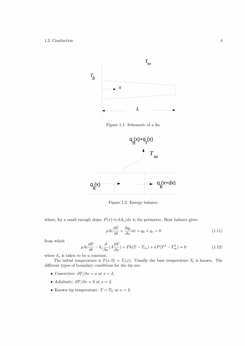
Consider the fin shown shown in Fig. 1.1. The energy flows are indicated in Fig. 1.2. Theconductive heat flow along the fin, the convective heat loss from the side, and the radiative loss fromthe side are
qk = −ksAdT
dx(1.8)
qh = hdAs(T − T∞) (1.9)
qr = σdAs(T4 − T 4
∞) (1.10)
2Also called the latent heat.
1.2. Conduction 4
T
T
b
∞
x
L
Figure 1.1: Schematic of a fin.
T∞
q (x)k
q (x+dx)k
q (x)+q (x)h r
Figure 1.2: Energy balance.
where, for a small enough slope, P (x) ≈ dAs/dx is the perimeter. Heat balance gives
ρAc∂T
∂t+∂qk∂x
dx+ qh + qr = 0 (1.11)
from which
ρAc∂T
∂t− ks
∂
∂x(A∂T
∂x) + Ph(T − T∞) + σP (T 4 − T 4
∞) = 0 (1.12)
where ks is taken to be a constant.The initial temperature is T (x, 0) = Ti(x). Usually the base temperature Tb is known. The
different types of boundary conditions for the tip are:
• Convective: ∂T/∂x = a at x = L
• Adiabatic: ∂T/∂x = 0 at x = L
• Known tip temperature: T = TL at x = L
1.2. Conduction 5
• Long fin: T = T∞ as x→ ∞
Taking
θ =T − T∞Tb − T∞
(1.13)
τ =kst
L2ρcFourier modulus (1.14)
ξ =x
L(1.15)
a(ξ) =A
Ab(1.16)
p(ξ) =P
Pb(1.17)
where the subscript indicates quantities at the base, the fin equation becomes
a∂θ
∂τ− ∂
∂ξ
(a∂θ
∂ξ
)+m2pθ + ǫp
[(θ + β)4 − β4
]= 0 (1.18)
where
m2 =PbhL
2
ksAb(1.19)
ǫ =σPbL
2(Tb − T∞)3
ksAb(1.20)
β =T∞
Tb − T∞(1.21)
1.2.3 Separation of variables
Steady-state coduction in a rectangular plate.
∇2T = 0 (1.22)
Let T (x, y) = X(x)Y (y).
1.2.4 Similarity variable
∂T
∂t= α
∂2T
∂x2(1.23)
1.2.5 Lumped-parameter approximation
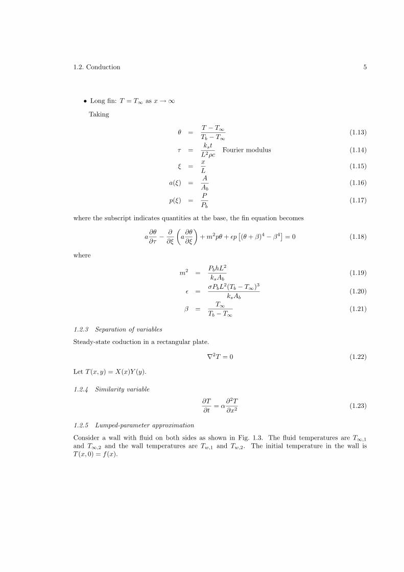
Consider a wall with fluid on both sides as shown in Fig. 1.3. The fluid temperatures are T∞,1
and T∞,2 and the wall temperatures are Tw,1 and Tw,2. The initial temperature in the wall isT (x, 0) = f(x).
1.2. Conduction 6
T∞,1
Tw,1
Tw,2
T∞,2
Figure 1.3: Wall with fluids on either side.
Steady state
In the steady state, we have
h1(T∞,1 − Tw,1) = ksTw,1 − Tw,2
L= h2(Tw,2 − T∞,2) (1.24)
from whichh1L
ks
T∞,1 − Tw,1
T∞,1 − T∞,2=
Tw,1 − Tw,2
T∞,1 − T∞,2=h2L
ks
Tw,2 − T∞,2
T∞,1 − T∞,2(1.25)
Thus we have
Tw,1 − Tw,2
T∞,1 − T∞,2≪ T∞,1 − Tw,1
T∞,1 − T∞,2ifh1L
ks≪ 1 (1.26)
Tw,1 − Tw,2
T∞,1 − T∞,2≪ Tw,2 − T∞,2
T∞,1 − T∞,2ifh2L
ks≪ 1 (1.27)
The Biot number is defined as
Bi =hL
ks(1.28)
Transient
∂T
∂t=ks
ρc
∂2T
∂x2(1.29)
There are two time scales: the short (conductive) tk0 = L2ρc/ks and the long (convective) th0 = Lρc/h.In the short time scale conduction within the slab is important, and convection from the sides isnot. In the long scale, the temperature within the slab is uniform, and changes due to convection.The ratio of the two tk0/t
h0 = Bi. In the long time scale it is possible to show that
LρscdT
dt+ h1(T − T∞,1) + h2(T − T∞,2) = 0 (1.30)
where T = Tw,1 = Tw,2.
1.3. Convection 7
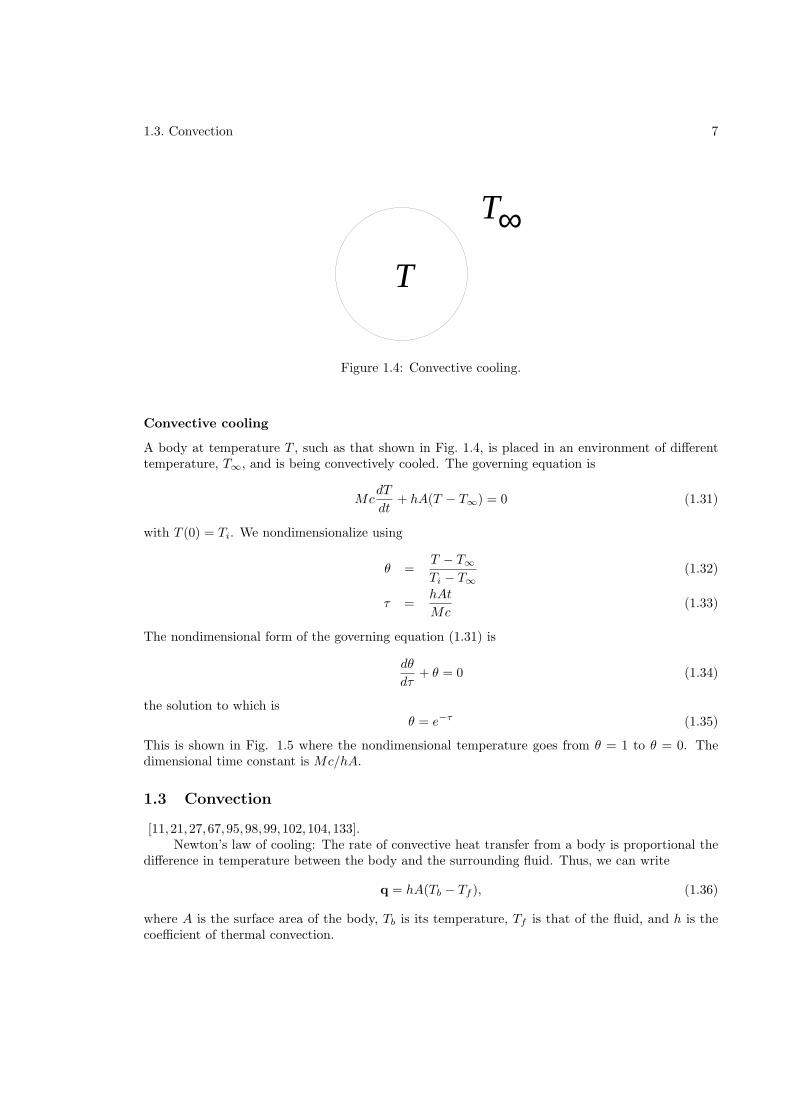
T∞T
Figure 1.4: Convective cooling.
Convective cooling
A body at temperature T , such as that shown in Fig. 1.4, is placed in an environment of differenttemperature, T∞, and is being convectively cooled. The governing equation is
McdT
dt+ hA(T − T∞) = 0 (1.31)
with T (0) = Ti. We nondimensionalize using
θ =T − T∞Ti − T∞
(1.32)
τ =hAt
Mc(1.33)
The nondimensional form of the governing equation (1.31) is
dθ
dτ+ θ = 0 (1.34)
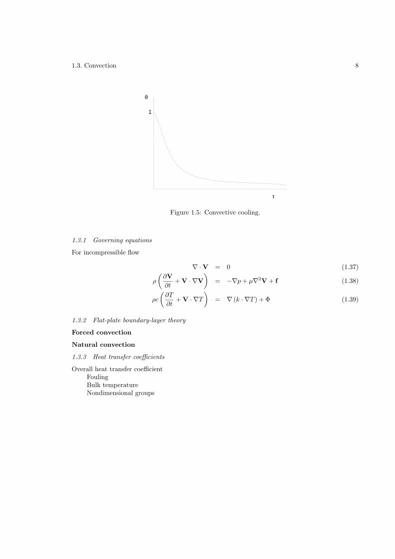
the solution to which isθ = e−τ (1.35)
This is shown in Fig. 1.5 where the nondimensional temperature goes from θ = 1 to θ = 0. Thedimensional time constant is Mc/hA.
1.3 Convection
[11, 21,27,67,95,98,99,102,104,133].Newton’s law of cooling: The rate of convective heat transfer from a body is proportional the
difference in temperature between the body and the surrounding fluid. Thus, we can write
q = hA(Tb − Tf ), (1.36)
where A is the surface area of the body, Tb is its temperature, Tf is that of the fluid, and h is thecoefficient of thermal convection.
1.3. Convection 8
θ
τ
1
Figure 1.5: Convective cooling.
1.3.1 Governing equations
For incompressible flow
∇ · V = 0 (1.37)
ρ
(∂V
∂t+ V · ∇V
)= −∇p+ µ∇2V + f (1.38)
ρc
(∂T
∂t+ V · ∇T
)= ∇ (k · ∇T ) + Φ (1.39)
1.3.2 Flat-plate boundary-layer theory
Forced convection
Natural convection
1.3.3 Heat transfer coefficients
Overall heat transfer coefficientFoulingBulk temperatureNondimensional groups
1.4. Radiation 9
Reynolds number Re =UL
ν(1.40)
Prandtl number =ν
κ(1.41)
Nusselt number Nu =hL
k(1.42)
Stanton number St = Nu/Pr Re (1.43)
Colburn j-factor j = St Pr2/3 (1.44)
Friction factor f =2τwρU2
(1.45)
1.4 Radiation
[25, 58,127,209]Emission can be from a surface or volumetric. Monochromatic radiation is at a single wave-
length. The direction distribution of radiation from a surface may be either specular (i.e. mirror-likewith angles of incidence and reflection equal) or diffuse (i.e. equal in all directions).
The spectral intensity of emission is the radiant energy leaving per unit time, unit area, unitwavelength, and unit solid angle. The emissive power is the emission of an entire hemisphere.Irradiations is the radiant energy coming in, while the radiosity is the energy leaving including theemission plus the reflection.
The absorptivity αλ, the reflectivity ρλ, and transmissivity τλ are all functions of the wavelkengthλ. Also
αλ + ρλ + τλ = 1 (1.46)
Integrating over all wavelengthsα+ ρ+ τ = 1 (1.47)
The emissivity is defined as
ǫλ =Eλ(λ, T )
Ebλ(λ, T )(1.48)
where the numerator is the actual energy emitted and the denominator is that that would have beenemitted by a blackbody at the same temperature. For the overall energy, we have a similar definition
ǫ =E(T )
Eb(T )(1.49)
so that the emission isE = ǫσT 4 (1.50)
For a gray body ǫλ is independent of λ.Kirchhoff’s law: αλ = ǫλ and α = ǫ.
1.4.1 Electromagnetic radiation
[173]
1.4. Radiation 10
Electromagnetic radiation travels at the speed of light c = 2.998× 10⁸ m/s. Thermal radiationis the part of the spectrum in the 0.1–100 µm range. The frequency f and wavelength λ of a waveare related by
c = fλ (1.51)
The radiation can also be considered a particles called phonons with energy
E = ~f (1.52)
where ~ is Planck’s constant.Maxwell’s equations of electromagnetic theory are
∇× H = J +∂D
∂t(1.53)
∇× E = −∂B∂t
(1.54)
∇ · D = ρ (1.55)
∇ · B = 0 (1.56)
where H, B, E, D, J, and ρ are the magnetic intensity, magnetic induction, electric field, electricdisplacement, current density, and charge density, respectively. For linear materials D = ǫE, J = gE(Ohm’s law), and B = µH, where ǫ is the permittivity, g is the electrical conductivity, and µ is thepermeability. For free space ǫ = 8.8542 × 10⁻¹² C2N−1m−2, and µ = 1.2566 × 10⁻⁶ NC−2s2,
For ρ = 0 and constant ǫ, g and µ, it can be shown that
∇2H − ǫµ∂2H
∂t2− gµ
∂H
∂t= 0 (1.57)
∇2E − ǫµ∂2E
∂t2− gµ
∂E
∂t= 0 (1.58)
The speed of an electromagnetic wave in free space is c = 1/√µǫ.
Blackbody radiation
Planck distribution [147]
Eλ =C1
λ5 [exp (C2/λT ) − 1](1.59)
Wien’s law: Putting dEλ/dλ = 0, the maximum of is seen to be at λ = λm, where
λmT = C3 (1.60)
and C3 = 2897.8 µmK.Stefan-Boltzmann’s law: The total radiation emitted is
Eb =
∫∞
0
Eλ dλ
= σT 4 (1.61)
where σ = 5.670 × 10⁻⁸ W/m2K4.
d2T
dx2= λ2T 4 (1.62)
1.5. Boiling and condensation 11
cold
hot
(a) parallel flow
cold
hot
(a) counter flow
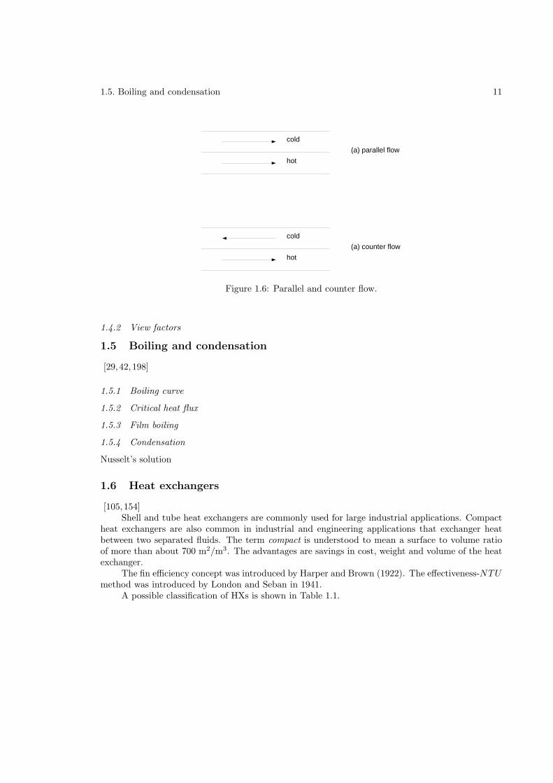
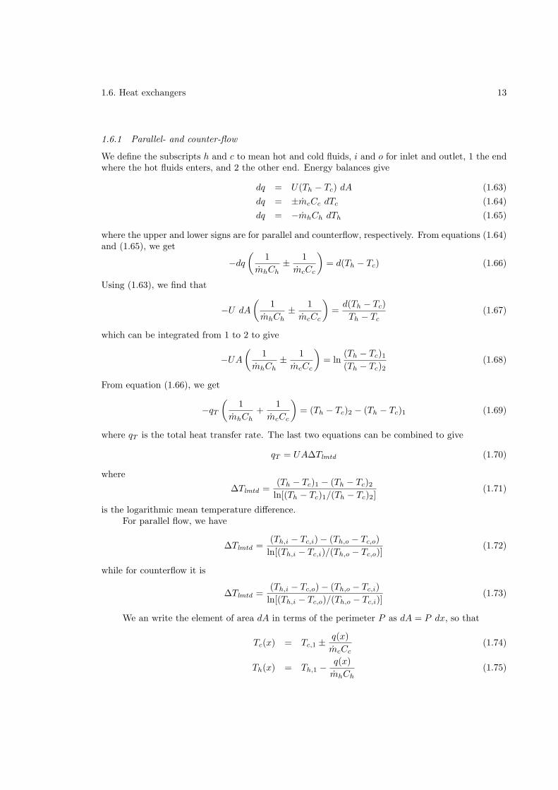
Figure 1.6: Parallel and counter flow.
1.4.2 View factors
1.5 Boiling and condensation
[29, 42,198]
1.5.1 Boiling curve
1.5.2 Critical heat flux
1.5.3 Film boiling
1.5.4 Condensation
Nusselt’s solution
1.6 Heat exchangers
[105,154]Shell and tube heat exchangers are commonly used for large industrial applications. Compact
heat exchangers are also common in industrial and engineering applications that exchanger heatbetween two separated fluids. The term compact is understood to mean a surface to volume ratioof more than about 700 m2/m3. The advantages are savings in cost, weight and volume of the heatexchanger.
The fin efficiency concept was introduced by Harper and Brown (1922). The effectiveness-NTUmethod was introduced by London and Seban in 1941.
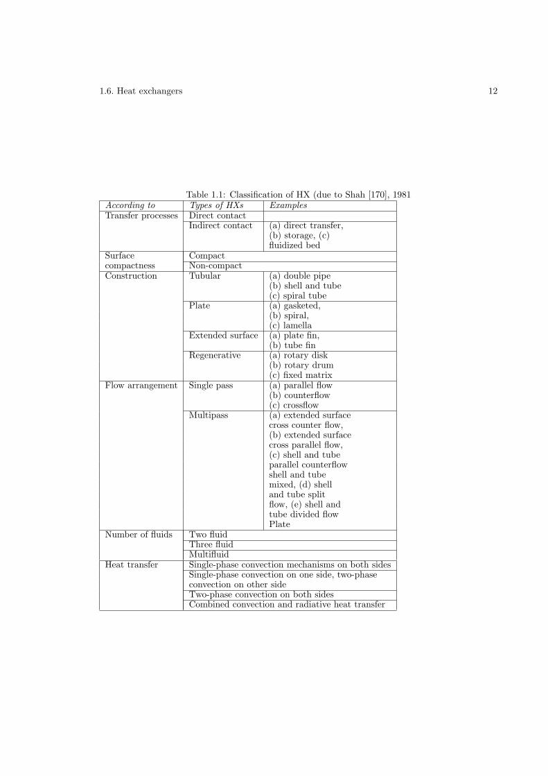
A possible classification of HXs is shown in Table 1.1.
1.6. Heat exchangers 12
Table 1.1: Classification of HX (due to Shah [170], 1981According to Types of HXs ExamplesTransfer processes Direct contact
Indirect contact (a) direct transfer,(b) storage, (c)fluidized bed
Surface Compactcompactness Non-compactConstruction Tubular (a) double pipe
(b) shell and tube(c) spiral tube
Plate (a) gasketed,(b) spiral,(c) lamella
Extended surface (a) plate fin,(b) tube fin
Regenerative (a) rotary disk(b) rotary drum(c) fixed matrix
Flow arrangement Single pass (a) parallel flow(b) counterflow(c) crossflow
Multipass (a) extended surfacecross counter flow,(b) extended surfacecross parallel flow,(c) shell and tubeparallel counterflowshell and tubemixed, (d) shelland tube splitflow, (e) shell andtube divided flowPlate
Number of fluids Two fluidThree fluidMultifluid
Heat transfer Single-phase convection mechanisms on both sidesSingle-phase convection on one side, two-phaseconvection on other sideTwo-phase convection on both sidesCombined convection and radiative heat transfer
1.6. Heat exchangers 13
1.6.1 Parallel- and counter-flow
We define the subscripts h and c to mean hot and cold fluids, i and o for inlet and outlet, 1 the endwhere the hot fluids enters, and 2 the other end. Energy balances give
dq = U(Th − Tc) dA (1.63)
dq = ±mcCc dTc (1.64)
dq = −mhCh dTh (1.65)
where the upper and lower signs are for parallel and counterflow, respectively. From equations (1.64)and (1.65), we get
−dq(
1
mhCh± 1
mcCc
)= d(Th − Tc) (1.66)
Using (1.63), we find that
−U dA
(1
mhCh± 1
mcCc
)=d(Th − Tc)
Th − Tc(1.67)
which can be integrated from 1 to 2 to give
−UA(
1
mhCh± 1
mcCc
)= ln
(Th − Tc)1(Th − Tc)2
(1.68)
From equation (1.66), we get
−qT(
1
mhCh+
1
mcCc
)= (Th − Tc)2 − (Th − Tc)1 (1.69)
where qT is the total heat transfer rate. The last two equations can be combined to give
qT = UA∆Tlmtd (1.70)
where
∆Tlmtd =(Th − Tc)1 − (Th − Tc)2
ln[(Th − Tc)1/(Th − Tc)2](1.71)
is the logarithmic mean temperature difference.For parallel flow, we have
∆Tlmtd =(Th,i − Tc,i) − (Th,o − Tc,o)
ln[(Th,i − Tc,i)/(Th,o − Tc,o)](1.72)
while for counterflow it is
∆Tlmtd =(Th,i − Tc,o) − (Th,o − Tc,i)
ln[(Th,i − Tc,o)/(Th,o − Tc,i)](1.73)
We an write the element of area dA in terms of the perimeter P as dA = P dx, so that
Tc(x) = Tc,1 ±q(x)
mcCc(1.74)
Th(x) = Th,1 −q(x)
mhCh(1.75)
1.6. Heat exchangers 14
Thusdq
dx+ qUP
(1
mhCh± 1
mcCc
)(1.76)
With the boundary condition q(0) = 0, the solution is
q9x) =Th,1 − Tc,11
mhCh± 1
mcCc
1 − exp
[−UP
(1
mhCh± 1
mcCc
)](1.77)
1.6.2 HX relations
The HX effectiveness is
ǫ =Q
Qmax(1.78)
=Ch(Th,i − Th,o)
Cmin(Th,i − Tc,i)(1.79)
=Cc(Tc,o − Tc,i)
Cmin(Th,i − Tc,i)(1.80)
whereCmin = min(Ch, Cc) (1.81)
Assuming U to be a constant, the number of transfer units is
NTU =AU
Cmin(1.82)
The heat capacity rate ratio is CR = Cmin/Cmax.
Effectiveness-NTU relations
In general, the effectiveness is a function of the HX configuration, its NTU and the CR of the fluids.(a) Counterflow
ǫ =1 − exp[−NTU(1 − CR)]
1 − CR exp[−NTU(1 − CR)](1.83)
so that ǫ→ 1 as NTU → ∞.(b) Parallel flow
ǫ =1 − exp[−NTU(1 − CR)]
1 + CR(1.84)
(c) Crossflow, both fluids unmixedSeries solution (Mason, 1954)
(d) Crossflow, one fluid mixed, the other unmixedIf the unmixed fluid has C = Cmin, then
ǫ = 1 − exp[−CR(1 − exp−NTUCr)] (1.85)
But if the mixed fluid has C = Cmin
ǫ = CR(1 − exp−CR(1 − e−NTU )) (1.86)
1.6. Heat exchangers 15
(e) Crossflow, both fluids mixed(f) Tube with wall temperature constant
ǫ = 1 − exp(−NTU) (1.87)
Pressure drop
It is important to determine the pressure drop through a heat exchanger. This is given by
∆p
p1=
G2
2ρ1p1
[(Kc + 1 − σ2) + 2(
ρ1
ρ2− 1) + f
Aρ1
Acρm− (1 − σ2 −Ke)
ρ1
ρ2
](1.88)
where Kc and Ke are the entrance and exit loss coefficients, and σ is the ratio of free-flow area tofrontal area.
1.6.3 Design methodology
Mean temperature-difference method
Given the inlet temperatures and flow rates, this method enables one to find the outlet temperatures,the mean temperature difference, and then the heat rate.
Effectiveness-NTU method
The order of calculation is NTU , ǫ, qmax and q.
1.6.4 Correlations
1.6.5 Extended surfaces
η0 = 1 − Af
A(1 − ηf ) (1.89)
where η0 is the total surface temperature effectiveness, ηf is the fin temperature effectiveness, Af isthe HX total fin area, and A is the HX total heat transfer area.
Problems
1. For a perimeter corresponding to a fin slope that is not small, derive Eq. 1.11.
2. The two sides of a plane wall are at temperatures T1 and T2. The thermal conductivity varies with temperaturein the form k(T ) = k0 + α(T − T1). Find the temperature distribution within the wall.
3. Consider a cylindrical pin fin of diameter D and length L. The base is at temperature Tb and the tip at T∞;the ambient temperature is also T∞. Find the steady-state temperature distribution in the fin, its effectiveness,and its efficiency. Assume that there is only convection but no radiation.
4. Show that the efficiency of the triangular fin shown in Fig. 1.7 is
ηf =1
mL
I1(2mL)
I0(2mL),
where m = (2h/kt)1/2, and I0 and I1 are the zeroth- and first-order Bessel functions of the first kind.
5. A constant-area fin between surfaces at temperatures T1 and T2 is shown in Fig. 1.8. If the external temperature,T∞(x), is a function of the coordinate x, find the general steady-state solution of the fin temperature T (x) interms of a Green’s function.
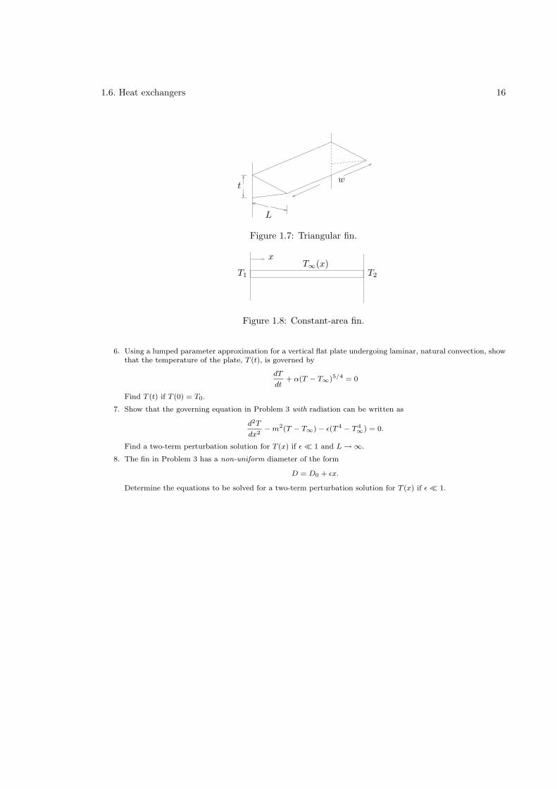
1.6. Heat exchangers 16
t
L
w
Figure 1.7: Triangular fin.
T2T1
T∞(x)x
Figure 1.8: Constant-area fin.
6. Using a lumped parameter approximation for a vertical flat plate undergoing laminar, natural convection, showthat the temperature of the plate, T (t), is governed by
dT
dt+ α(T − T∞)5/4 = 0
Find T (t) if T (0) = T0.
7. Show that the governing equation in Problem 3 with radiation can be written as
d2T
dx2− m2(T − T∞) − ǫ(T 4 − T 4
∞) = 0.
Find a two-term perturbation solution for T (x) if ǫ ≪ 1 and L → ∞.
8. The fin in Problem 3 has a non-uniform diameter of the form
D = D0 + ǫx.
Determine the equations to be solved for a two-term perturbation solution for T (x) if ǫ ≪ 1.
Part II
No spatial dimension
17
Chapter 2
Dynamics
2.1 Variable heat transfer coefficient
If, however, the h is slightly temperature-dependent, then we have
dθ
dτ+ (1 + ǫθ)θ = 0 (2.1)
which can be solved by the method of perturbations. We assume that
θ(τ) = θ0(τ) + ǫθ1(τ) + ǫ2θ2(τ) + . . . (2.2)
To order ǫ0, we have
dθ0dτ
+ θ0 = 0 (2.3)
θ0(0) = 1 (2.4)
which has the solutionθ0 = e−τ (2.5)
To the next order ǫ1, we get
dθ1dτ
+ θ1 = −θ20 (2.6)
= −e−2τ (2.7)
θ1(0) = 0 (2.8)
the solution to which isθ1 = −e−t + e−2τ (2.9)
Taking the expansion to order ǫ2
dθ2dτ
+ θ2 = −2θ0θ1 (2.10)
= −2e−2t − 2e−3τ (2.11)
θ2(0) = 1 (2.12)
18
2.1. Variable heat transfer coefficient 19
with the solutionθ2 = e−τ − 2e−2τ + e−3τ (2.13)
And so on. Combining, we get
θ = e−τ − ǫ(e−τ − e−2τ ) + ǫ2(e−τ − 2e−2τ + e−3τ ) + . . . (2.14)
Alternatively, we can find an exact solution to equation (2.1). Separating variables, we get
dθ
(1 + ǫθ)θ= dτ (2.15)
Integrating
lnθ
ǫθ + 1= −τ + C (2.16)
The condition θ(0) = 1 gives C = − ln(1 + ǫ), so that
lnθ(1 + ǫ)
1 + ǫθ= −τ (2.17)
This can be rearranged to give
θ =e−τ
1 + ǫ(1 − e−τ )(2.18)
A Taylor-series expansion of the exact solution gives
θ = e−τ[1 + ǫ(1 − e−τ
]−1
(2.19)
= e−τ[1 − ǫ(1 − e−τ ) + ǫ2(1 − e−τ )2 + . . .
](2.20)
= e−τ − ǫ(e−τ − e−2τ ) + ǫ2(e−τ − 2e−2τ + e−3τ ) + . . . (2.21)
2.1.1 Radiative cooling
If the heat loss is due to radiation, we can write
McdT
dt+ σA(T 4 − T 4
∞) = 0 (2.22)
Taking the dimensionless temperature to be defined in equation (1.32), and time to be
τ =σA(Ti − T∞)3t
Mc(2.23)
and introducing the parameter
β =T∞
Ti − T∞(2.24)
we getdφ
dτ+ φ4 = β4 (2.25)
whereφ = θ + β (2.26)
2.1. Variable heat transfer coefficient 20
Writing the equation asdφ
φ4 − β4= −dτ (2.27)
the integral is1
4β3ln
(φ− β
φ+ β
)− 1
2β3tan−1
(φ
β
)= −τ + C (2.28)
Using the initial condition θ(0) = 1, we get (?)
τ =1
2β3
[1
2ln
(β + T )(β − 1)
(β − T )(β + 1)+ tan−1 T − 1
β + (T/β)
](2.29)
2.1.2 Convective with weak radiation
The governing equationis
McdT
dt+ hA(T − T∞) + σA(T 4 − T 4
∞) = 0 (2.30)
with T (0) = Ti. Using the variables defined by equations (1.32) and (1.33), we get
dθ
dτ+ θ + ǫ
[(θ + β4)4 − β4
]= 0 (2.31)
where β is defined in equation (2.24), and
ǫ =σ(Ti − T∞)3
h(2.32)
If radiative effects are small compared to the convective (for Ti − T∞ = 100 K and h = 10 W/m2Kwe get ǫ = 5.67 × 10⁻³), we can take ǫ≪ 1. Substituting the perturbation series, equation (2.2), inequation (2.31), we get
d
dτ
(θ0 + ǫθ1 + ǫ2θ2 + . . .
)+(θ0 + ǫθ1 + ǫ2θ2 + . . .
)
+ǫ[ (θ0 + ǫθ1 + ǫ2θ2 + . . .
)4+ 4β
(θ0 + ǫθ1 + ǫ2θ2 + . . .
)3
+6β2(θ0 + ǫθ1 + ǫ2θ2 + . . .
)24β3
(θ0 + ǫθ1 + ǫ2θ2 + . . .
) ]= 0 (2.33)
In this case
dθ
dτ+ (θ − θ0) + ǫ(θ4 − θ4s) = 0 (2.34)
θ(0) = 1 (2.35)
As a special case, of we take β = 0, i.e. T∞ = 0, we get
dθ
dτ+ θ + ǫθ4 = 0 (2.36)
which has an exact solution
τ =1
3ln
1 + ǫθ3
(1 + ǫ)θ3(2.37)
2.2. Radiation in an enclosure 21
2.2 Radiation in an enclosure
Consider a closed enclosure with N walls radiating to each other and with a central heater H. Thewalls have no other heat loss and have different masses and specific heats. The governing equationsare
MicidTi
dt+ σ
N∑
j=1
AiFij(T4i − T 4
j ) + σAiFiH(T 4i − T 4
H) = 0 (2.38)
where the view factor Fij is the fraction of radiation leaving surface i that falls on j. The steadystate is
T i = TH (i = 1, . . . , N) (2.39)
Linear stability is determined by a small perturbation of the type
Ti = TH + T ′
i (2.40)
from which
MicidT ′
i
dt+ 4σT 3
H
N∑
j=1
AiFij(T′
i − T ′
j) + 4σT 3HAiFiHT
′
i = 0 (2.41)
This can be written as
MdT′
dt= −4σT 3
HAT′ (2.42)
2.3 Long time behavior
The general form of the equation for heat loss from a body with internal heat generation is
dθ
dτ+ f(θ) = a (2.43)
with θ(0) = 1. Letf(θ) = a (2.44)
Then we would like to show that θ → θ as t→ ∞. Writing
θ = θ + θ′ (2.45)
we havedθ′
dτ+ f(θ + θ′) = a (2.46)
2.3.1 Linear analysis
If we assume that θ′ is small, then a Taylor series gives
f(θ + θ′) = f(θ) + θ′f ′(θ) + . . . (2.47)
from whichdθ′
dτ+ bθ′ = 0 (2.48)
where b = f ′(θ). The solution isθ′ = Ce−bτ (2.49)
so that θ′ → 0 as t→ ∞ if b > 0.
2.4. Time-dependent T∞ 22
2.3.2 Nonlinear analysis
Multiplying equation (2.46) by θ′, we get
1
2
d
dτ(θ′)2 = −θ′
[f(θ + θ′) − f(θ)
](2.50)
Thusd
dτ(θ′)2 ≤ 0 (2.51)
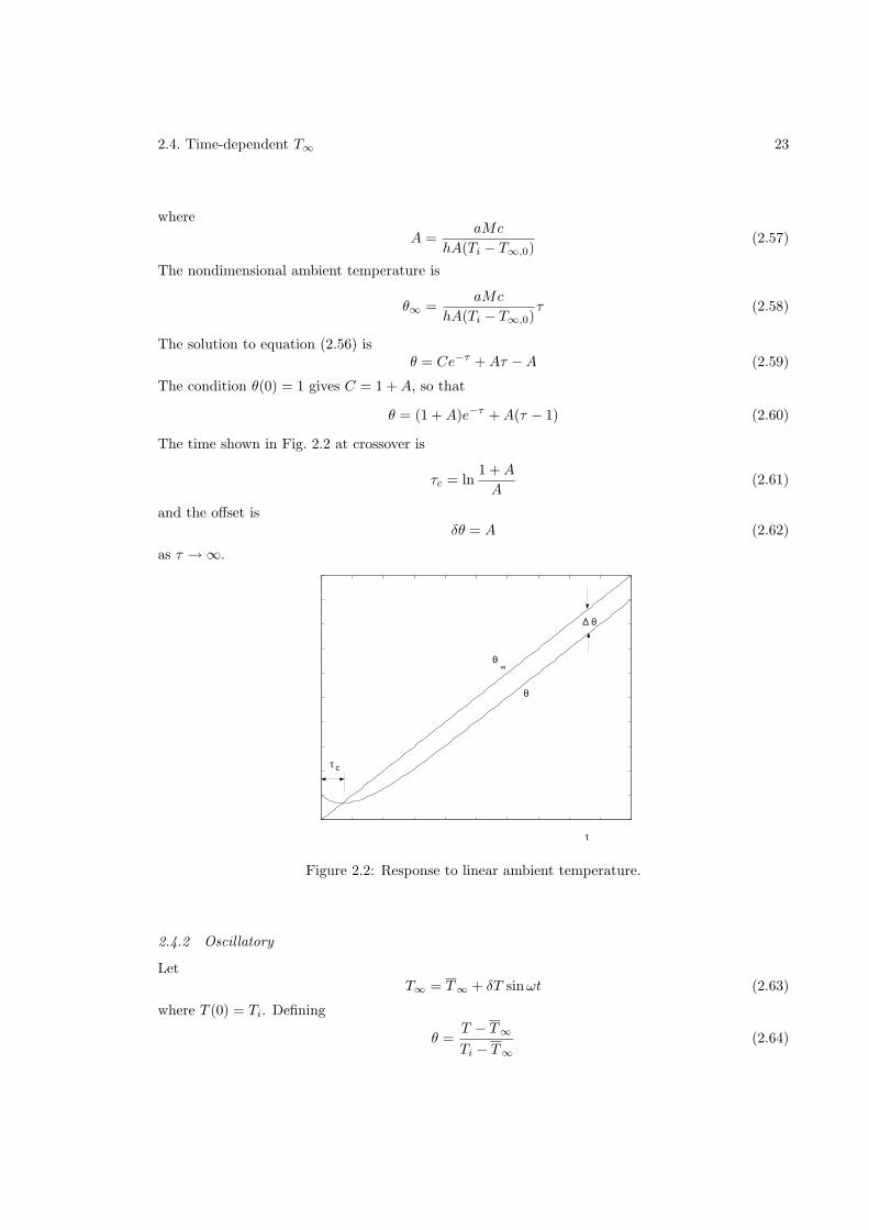
if θ′ and [f(θ + θ′) − f(θ)], as shown in Fig. 2.1, are both of the same sign or zero. Thus θ′ → 0 asτ → ∞.
f( )θ
θ
f( )θ
θ
Figure 2.1: Convective cooling.
2.4 Time-dependent T∞
Let
McdT
dt+ hA(T − T∞(t)) = 0 (2.52)
withT (0) = Ti (2.53)
2.4.1 Linear
LetT∞ = T∞,0 + at (2.54)
Defining the nondimensional temperature as
θ =T − T∞,0
Ti − T∞,0(2.55)
and time as in equation (1.33), we getdθ
dτ+ θ = Aτ (2.56)
2.4. Time-dependent T∞ 23
where
A =aMc
hA(Ti − T∞,0)(2.57)
The nondimensional ambient temperature is
θ∞ =aMc
hA(Ti − T∞,0)τ (2.58)
The solution to equation (2.56) isθ = Ce−τ +Aτ −A (2.59)
The condition θ(0) = 1 gives C = 1 +A, so that
θ = (1 +A)e−τ +A(τ − 1) (2.60)
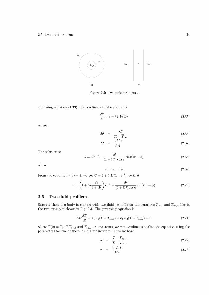
The time shown in Fig. 2.2 at crossover is
τc = ln1 +A
A(2.61)
and the offset isδθ = A (2.62)
as τ → ∞.
θ
θ∞
∆
θ
τ
τ c
Figure 2.2: Response to linear ambient temperature.
2.4.2 Oscillatory
LetT∞ = T∞ + δT sinωt (2.63)
where T (0) = Ti. Defining
θ =T − T∞
Ti − T∞
(2.64)
2.5. Two-fluid problem 24
T∞,1
∞,2T
∞,2T T∞,1T
T
(a) (b)
Figure 2.3: Two-fluid problems.
and using equation (1.33), the nondimensional equation is
dθ
dτ+ θ = δθ sin Ωτ (2.65)
where
δθ =δT
Ti − T∞
(2.66)
Ω =ωMc
hA(2.67)
The solution is
θ = Ce−τ +δθ
(1 + Ω2) cosφsin(Ωτ − φ) (2.68)
whereφ = tan−1 Ω (2.69)
From the condition θ(0) = 1, we get C = 1 + δΩ/(1 + Ω2), so that
θ =
(1 + δθ
Ω
1 + Ω2
)e−τ +
δθ
(1 + Ω2) cosφsin(Ωτ − φ) (2.70)
2.5 Two-fluid problem
Suppose there is a body in contact with two fluids at different temperatures T∞,1 and T∞,2, like inthe two examples shown in Fig. 2.3. The governing equation is
McdT
dt+ h1A1(T − T∞,1) + h2A2(T − T∞,2) = 0 (2.71)
where T (0) = Ti. If T∞,1 and T∞,2 are constants, we can nondimensionalize the equation using theparameters for one of them, fluid 1 for instance. Thus we have
θ =T − T∞,1
Ti − T∞,1(2.72)
τ =h1A1t
Mc(2.73)
2.6. Two-body problem 25
from whichdθ
dτ+ θ + α(θ + β) = 0 (2.74)
with θ(0) = 1, where
α =h2A2
h1A1(2.75)
β =T∞,1 − T∞,2
Ti − T∞,1(2.76)
The equation can be written asdθ
dτ+ (1 + α)θ = −αβ (2.77)
with the solution
θ = Ce−(1+α)τ − αβ
1 + α(2.78)
The condition θ(0) = 1 gives C = 1 + αβ/(1 + α), from which
θ =
(1 +
αβ
1 + α
)e−(1+α)τ − αβ
1 + α(2.79)
For α = 0, the solution reduces to the single-fluid case, equation (1.35). Otherwise the time constantof the general system is
t0 =Mc
h1A1 + h2A2(2.80)
2.6 Two-body problem
2.6.1 Convective
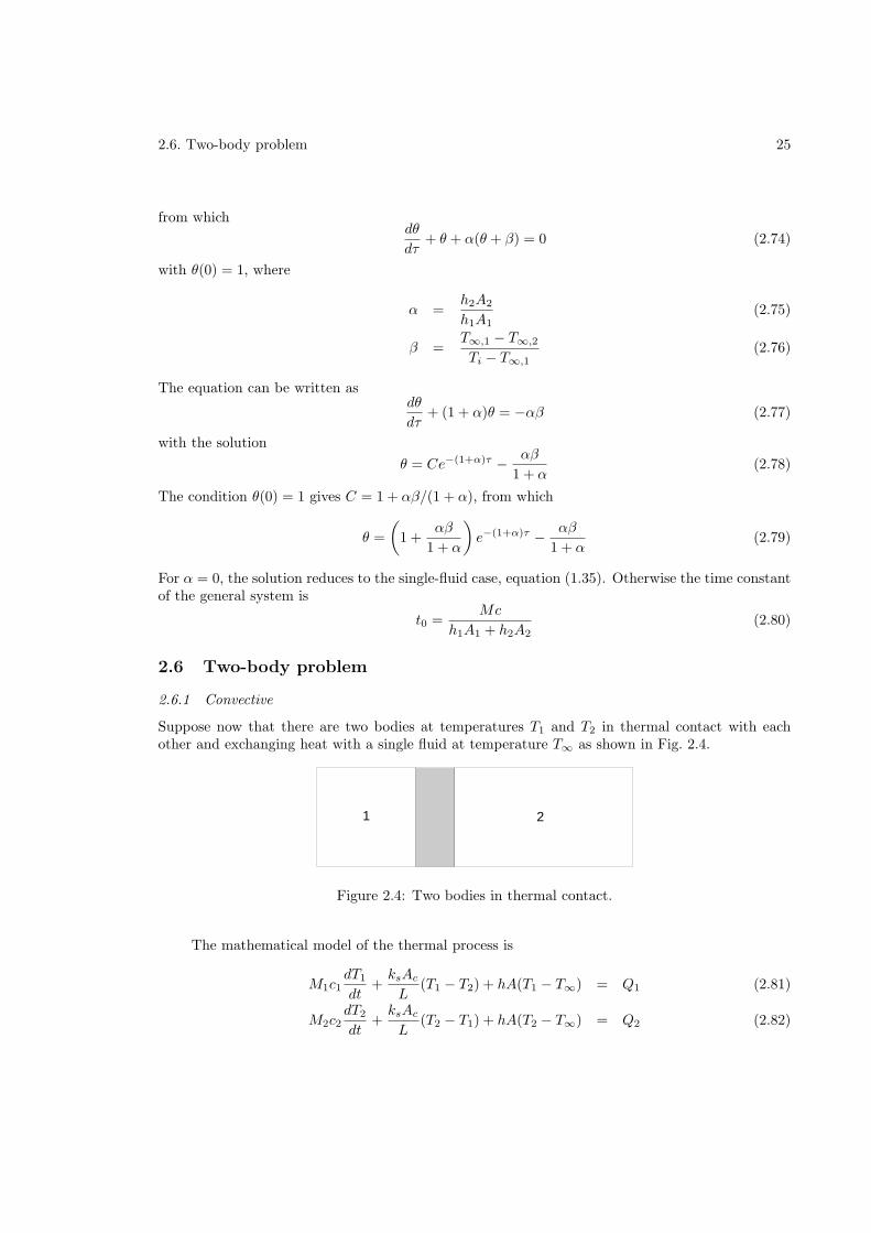
Suppose now that there are two bodies at temperatures T1 and T2 in thermal contact with eachother and exchanging heat with a single fluid at temperature T∞ as shown in Fig. 2.4.
1 2
Figure 2.4: Two bodies in thermal contact.
The mathematical model of the thermal process is
M1c1dT1
dt+ksAc
L(T1 − T2) + hA(T1 − T∞) = Q1 (2.81)
M2c2dT2
dt+ksAc
L(T2 − T1) + hA(T2 − T∞) = Q2 (2.82)
2.6. Two-body problem 26
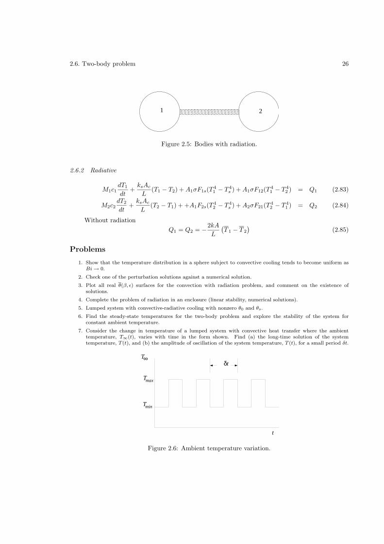
1 2
Figure 2.5: Bodies with radiation.
2.6.2 Radiative
M1c1dT1
dt+ksAc
L(T1 − T2) +A1σF1s(T
41 − T 4
s ) +A1σF12(T41 − T 4
2 ) = Q1 (2.83)
M2c2dT2
dt+ksAc
L(T2 − T1) + +A1F2s(T
42 − T 4
s ) +A2σF21(T42 − T 4
1 ) = Q2 (2.84)
Without radiation
Q1 = Q2 = −2kA
L
(T 1 − T 2
)(2.85)
Problems
1. Show that the temperature distribution in a sphere subject to convective cooling tends to become uniform asBi → 0.
2. Check one of the perturbation solutions against a numerical solution.
3. Plot all real θ(β, ǫ) surfaces for the convection with radiation problem, and comment on the existence ofsolutions.
4. Complete the problem of radiation in an enclosure (linear stability, numerical solutions).
5. Lumped system with convective-radiative cooling with nonzero θ0 and θs.
6. Find the steady-state temperatures for the two-body problem and explore the stability of the system forconstant ambient temperature.
7. Consider the change in temperature of a lumped system with convective heat transfer where the ambienttemperature, T∞(t), varies with time in the form shown. Find (a) the long-time solution of the systemtemperature, T (t), and (b) the amplitude of oscillation of the system temperature, T (t), for a small period δt.
t
T∞
Tmax
Tmin
δt
Figure 2.6: Ambient temperature variation.
Chapter 3
Control
3.1 Introduction
There are many kinds of thermal systems in common industrial, transportation and domestic usethat need to be controlled in some manner, and there are many ways in which that can be done.One can give the example of heat exchangers [85, 114], environmental control in buildings [70, 72,82,115,152,218], satellites [101,172,184,221], thermal packaging of electronic components [150,185],manufacturing [54], rapid thermal processing of computer chips [84, 158, 200], and many others. Ifprecise control is not required, or if the process is very slow, control may simply be manual; otherwisesome sort of mechanical or electrical feedback system has to be put in place for it to be automatic.
Most thermal systems are generally complex involving diverse physical processes. These includenatural and forced convection, radiation, complex geometries, property variation with temperature,nonlinearities and bifurcations, hydrodynamic instability, turbulence, multi-phase flows, or chemicalreaction. It is common to have large uncertainties in the values of heat transfer coefficients, ap-proximations due to using lumped parameters instead of distributed temperature fields, or materialproperties that may not be accurately known. In this context, a complex system can be defined asone that is made up of sub-systems, each one of which can be analyzed and computed, but when puttogether presents such a massive computational problem so as to be practically intractable. For thisreason large, commonly used engineering systems are hard to model exactly from first principles,and even when this is possible the dynamic responses of the models are impossible to determinecomputationally in real time. Most often some degree of approximation has to be made to themathematical model. Approximate correlations from empirical data are also heavily used in prac-tice. The two major reasons for which control systems are needed to enable a thermal system tofunction as desired are the approximations used during design and the existence of unpredictableexternal and internal disturbances which were not taken into account.
There are many aspects of thermal control that will not be treated in this brief review. The mostimportant of these are hardware considerations; all kinds of sensors and actuators [59,187] developedfor measurement and actuation are used in the control of thermal systems. Many controllers arealso computer based, and the use of microprocessors [87, 180] and PCs in machines, devices andplants is commonplace. Flow control, which is closely related to and is often an integral part ofthermal control, has its own extensive literature [64]. Discrete-time (as opposed to continuous-time) systems will not be described. The present paper will, however, concentrate only on thebasic principles relating to the theory of control as applied to thermal problems, but even then itwill be impossible to go into any depth within the space available. This is only an introduction,
27
3.2. Systems 28
-p -
? ?
u(t)x(t)
plant
y(t)
w(t) λ
Figure 3.1: Schematic of a system withoutcontroller.
-e(t) controller -p -
??
u(t)x(t)
plant
y(t)
w(t) λ
jC?-yr(t)
Figure 3.2: Schematic of a system with com-parator C and controller.
and the interested reader should look at the literature that is cited for further details. There aregood texts and monographs available on the basics of control theory [116, 132, 144, 157], processcontrol [28,75,93,151], nonlinear control [91], infinite-dimensional systems [39,89], and mathematicsof control [9, 179] that can be consulted. These are all topics that include and are included withinthermal control.
3.2 Systems
Some basic ideas of systems will be defined here even though, because of the generality involved, itis hard to be specific at this stage.
3.2.1 Systems without control
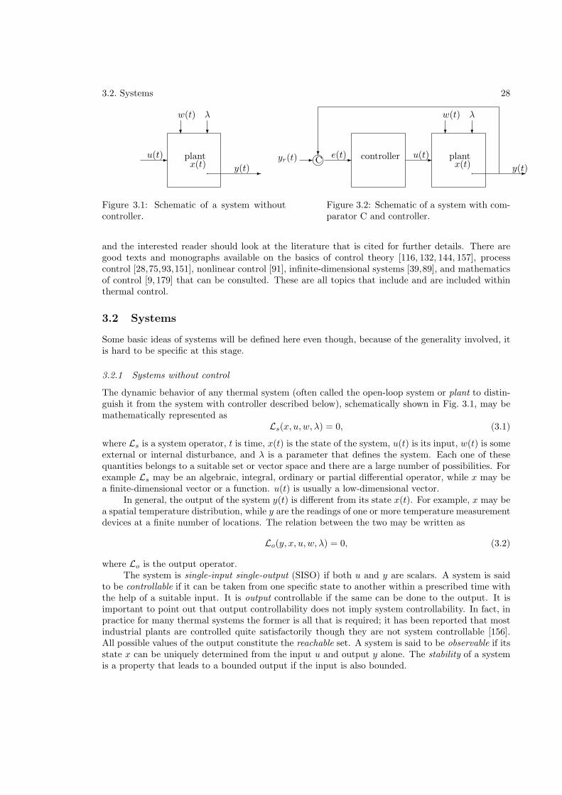
The dynamic behavior of any thermal system (often called the open-loop system or plant to distin-guish it from the system with controller described below), schematically shown in Fig. 3.1, may bemathematically represented as
Ls(x, u, w, λ) = 0, (3.1)
where Ls is a system operator, t is time, x(t) is the state of the system, u(t) is its input, w(t) is someexternal or internal disturbance, and λ is a parameter that defines the system. Each one of thesequantities belongs to a suitable set or vector space and there are a large number of possibilities. Forexample Ls may be an algebraic, integral, ordinary or partial differential operator, while x may bea finite-dimensional vector or a function. u(t) is usually a low-dimensional vector.
In general, the output of the system y(t) is different from its state x(t). For example, x may bea spatial temperature distribution, while y are the readings of one or more temperature measurementdevices at a finite number of locations. The relation between the two may be written as
Lo(y, x, u, w, λ) = 0, (3.2)
where Lo is the output operator.The system is single-input single-output (SISO) if both u and y are scalars. A system is said
to be controllable if it can be taken from one specific state to another within a prescribed time withthe help of a suitable input. It is output controllable if the same can be done to the output. It isimportant to point out that output controllability does not imply system controllability. In fact, inpractice for many thermal systems the former is all that is required; it has been reported that mostindustrial plants are controlled quite satisfactorily though they are not system controllable [156].All possible values of the output constitute the reachable set. A system is said to be observable if itsstate x can be uniquely determined from the input u and output y alone. The stability of a systemis a property that leads to a bounded output if the input is also bounded.
3.3. Linear systems theory 29
3.2.2 Systems with control
The objective of control is to have a given output y = yr(t), where the reference or set value yr isprescribed. The problem is called regulation if yr is a constant, and tracking if it is function of time.
In open-loop control the input is selected to give the desired output without using any infor-mation from the output side; that is one would have to determine u(t) such that y = yr(t) usingthe mathematical model of the system alone. This is a passive method of control that is used inmany thermal systems. It will work if the behavior of the system is exactly predictable, if preciseoutput control is not required, or if the output of the system is not very sensitive to the input. Ifthe changes desired in the output are very slow then manual control can be carried out, and thatis also frequently done. A self-controlling approach that is sometimes useful is to design the systemin such a way that any disturbance will bring the output back to the desired value; the output ineffect is then insensitive to changes in input or disturbances.
Open-loop control is not usually effective for many systems. For thermal systems contributingfactors are the uncertainties in the mathematical model of the plant and the presence of unpredictabledisturbances. Internal disturbances may be noise in the measuring or actuating devices or a changein surface heat transfer characteristics due to fouling, while external ones may be a change in theenvironmental temperature. For these cases closed-loop control is an appropriate alternative. Thisis done using feedback from the output, as measured by a sensor, to the input side of the system, asshown in Fig. 3.2; the figure actually shows unit feedback. There is a comparator which determinesthe error signal e(t) = e(yr, y), which is usually taken to be
e = yr − y. (3.3)
The key role is played by the controller which puts out a signal that is used to move an actuator inthe plant.
Sensors that are commonly used are temperature-measuring devices such as thermocouples,resistance thermometers or thermistors. The actuator can be a fan or a pump if the flow rate is tobe changed, or a heater if the heating rate is the appropriate variable. The controller itself is eitherentirely mechanical if the system is not very complex, or is a digital processor with appropriatesoftware. In any case, it receives the error in the output e(t) and puts out an appropriate controlinput u(t) that leads to the desired operation of the plant.
The control process can be written as
Lc(u, e, λ) = 0, (3.4)
where Lc is a control operator. The controller designer has to propose a suitable Lc, and then Eqs.(C.9)–(3.4) form a set of equations in the unknowns x(t), y(t) and u(t). Choice of a control strategydefines Lo and many different methodologies are used in thermal systems. It is common to use on-off(or bang-bang, relay, etc.) control. This is usually used in heating or cooling systems in which theheat coming in or going out is reduced to zero when a predetermined temperature is reached andset at a constant value at another temperature. Another method is Proportional-Integral-Derivative(PID) control [214] in which
u = Kpe(t) +Ki
∫ t
0
e(s) ds+Kdde
dt. (3.5)
3.3 Linear systems theory
The term classical control is often used to refer to theory derived on the basis of Laplace transforms.Since this is exclusively for linear systems, we will be using the so-called modern control or state-
3.3. Linear systems theory 30
space analysis which is based on dynamical systems, mainly because it can be extended to nonlinearsystems. Where they overlap, the issue is only one of preference since the results are identical.Control theory can be developed for different linear operators, and some of these are outlined below.
3.3.1 Ordinary differential equations
Much is known about a linear differential system in which Eqs. (C.9) and (3.2) take the form
dx
dt= Ax+Bu, (3.6)
y = Cx+Du, (3.7)
where x ∈ Rn, u ∈ R
m, y ∈ Rp, A ∈ R
n×n, B ∈ Rn×m, C ∈ R
p×n, D ∈ Rp×m. x, u and y are
vectors of different lengths and A, B, C, and D are matrices of suitable sizes. Though A, B, C, andD can be functions of time in general, here they will be treated as constants.
The solution of Eq. (3.6) is
x(t) = eA(t−t0)x(t0) +
∫ t
t0
eA(t−s)Bu(s) ds. (3.8)
where the exponential matrix is defined as
eAt = I +At+1
2!A2t2 +
1
3!A3t3 + . . . ,
with I being the identity matrix. From Eq. (3.7), we get
y(t) = C
[eAtx(t0) +
∫ t
t0
eA(t−s) Bu(s) ds
]+Du. (3.9)
Eqs. (3.8) and (3.9) define the state x(t) and output y(t) if the input u(t) is given.It can be shown that for the system governed by Eq. (3.6), a u(t) can be found to take x(t)
from x(t0) at t = t0 to x(tf ) = 0 at t = tf if and only if the matrix
M =
[B
... AB... A2B
... . . .... An−1B
]∈ R
n×nm (3.10)
is of rank n. The system is then controllable. For a linear system, controllability from one state toanother implies that the system can be taken from any state to any other. It must be emphasizedthat the u(t) that does this is not unique.
Similarly, it can be shown that the output y(t) is controllable if and only if
N =
[D
... CB... CAB
... CA2B... . . .
... CAn−1B
]∈ R
p×(n+1)m (3.11)
is of rank p. Also, the state x(t) is observable if and only if the matrix
P =
[C
... CA... CA2 . . .
... CAn−1
]T
∈ Rpn×n (3.12)
is of rank n.
3.4. Nonlinear aspects 31
3.3.2 Algebraic-differential equations
This is a system of equations of the form
Edx
dt= A x+B u, (3.13)
where the matrix E ∈ Rn×n is singular [113]. This is equivalent to a set of equations, some of which
are ordinary differential and the rest are algebraic. As a result of this, Eq. (3.13) cannot be convertedinto (3.6) by substitution. The index of the system is the least number of differentiations of thealgebraic equations that is needed to get the form of Eq. (3.6). The system may not be completelycontrollable since some of the components of x are algebraically related, but it may have restrictedor R-controllability [45].
3.4 Nonlinear aspects
The following are a few of the issues that arise in the treatment of nonlinear thermal control problems.
3.4.1 Models
There are no general mathematical models for thermal systems, but one that can be used is ageneralization of Eq. (3.6) such as
dx
dt= f(x, u). (3.14)
where f : Rn × R
m 7→ Rn. If one is interested in local behavior about an equilibrium state x = x0,
u = 0, this can be linearized in that neighborhood to give
dx
dt=
∂f
∂x
∣∣∣∣∣0
x′ +∂f
∂u
∣∣∣∣∣0
u′
= Ax′ +Bu′, (3.15)
where x = x0 + x′ and u = u′. The Jacobian matrices (∂f/∂x)0 and (∂f/∂u)0, are evaluated at theequilibrium point. Eq. (3.15) has the same form as Eq. (3.6).
3.4.2 Controllability and reachability
General theorems for the controllability of nonlinear systems are not available at this point in time.Results obtained from the linearized equations generally do not hold for the nonlinear equations.The reason is that in the nonlinear case one can take a path in state space that travels far from theequilibrium point and then returns close to it. Thus regions of state space that are unreachable withthe linearized equations may actually be reachable. In a thermal convection loop it is possible to gofrom one branch of a bifurcation solution to another in this fashion [1].
3.4.3 Bounded variables
In practice, due to hardware constraints it is common to have the physical variables confined tocertain ranges, so that variables such as x and u in Eqs. (C.9) and (3.2), being temperatures, heatrates, flow rates and the like, are bounded. If this happens, even systems locally governed by Eqs.(3.6) and (3.7) are now nonlinear since the sum of solutions may fall outside the range in which x
3.5. System identification 32
exists and thus may not be a valid solution. On the other hand, for a controllable system in whichonly u is bounded in a neighborhood of zero, x can reach any point in R
n if the eigenvalues of A havezero or positive real parts, and the origin is reachable if the eigenvalues of A have zero or negativereal parts [179].
3.4.4 Relay and hysteresis
A relay is an element of a system that has an input-output relationship that is not smooth; it may bediscontinuous or not possess first or higher-order derivatives. This may be accompanied by hysteresiswhere the relationship also depends on whether the input is increasing or decreasing. Valves aretypical elements in flow systems that have this kind of behavior.
3.5 System identification
To be able to design appropriate control systems, one needs to have some idea of the dynamicbehavior of the thermal system that is being controlled. Mathematical models of these systemscan be obtained in two entirely different ways: from first principles using known physical laws, andempirically from the analysis of experimental information (though combinations of the two pathsare not only possible but common). The latter is the process of system identification, by which acomplex system is reduced to mathematical form using experimental data [75, 121, 129]. There aremany different ways in which this can be done, the most common being the fitting of parameters toproposed models [141]. In this method, a form of Ls is assumed with unknown parameter values.Through optimization routines the values of the unknowns are chosen to obtain the best fit of theresults of the model with experimental information. Apart from the linear Eq. (3.6), other modelsthat are used include the following.
• There are many forms based on Eq. (3.14), one of which is the closed-affine model
dx
dt= F1(x) + F2(x)u (3.16)
The bilinear equation for which F1(x) = Ax and F2(x) = Nx+ b is a special case of this.
• Volterra models, like
y(t) = y0(t) +
∞∑
i=1
∫∞
−∞
. . .
∫∞
−∞
ki(t; t1, t2, t3, . . . , ti)u(t1) . . . u(ti) dt1 . . . dti (3.17)
for a SISO system, are also used.
• Functional [71], difference [23] or delay [57] equations such as
dx
dt= A x(t− s) +B u (3.18)
also appear in the modeling of thermal systems.
• Fractional-order derivatives, of which there are several different possible definitions [10,17,134,135, 148] can be used in differential models. As an example, the Riemann-Liouville definitionof the nth derivative of f(t) is
aDnt f(t) =
1
Γ(m− n+ 1)
dm+1
dtm+1
∫ t
a
(t− s)m−nf(s) ds, (3.19)
where a and n are real numbers and m is the largest integer smaller than n.
3.6. Control strategies 33
3.6 Control strategies
3.6.1 Mathematical model
Consider a body that is cooled from its surface by convection to the environment with a constantambient temperature T∞. It also has an internal heat source Q(t) to compensate for this heat loss,and the control objective is to maintain the temperature of the body at a given level by manipulatingthe heat source. The Biot number for the body is Bi = hL/k, where h is the convective heat transfercoefficient, L is a characteristics length dimension of the body, and k is its thermal conductivity.If Bi < 0.1, the body can be considered to have a uniform temperature T (t). Under this lumpedapproximation the energy balance is given by
McdT
dt+ hAs(T − T∞) = Q(t), (3.20)
where M is the mass of the body, c is its specific heat, and As is the surface area for convection.UsingMc/hAs and hAs(Ti−T∞) as the characteristic time and heat rate, this equation becomes
dθ
dt+ θ = Q(t) (3.21)
Here θ = (T − T∞)/(Ti − T∞) where T (0) = Ti so that θ(0) = 1. The other variables are now non-dimensional. With x = θ, u = Q, n = m = 1 in Eq. (3.6), we find from Eq. (3.10) that rank(M)=1,so the system is controllable.
Open-loop operation to maintain a given non-dimensional temperature θr is easily calculated.Choosing Q = θr, it can be shown from the solution of Eq. (3.21), that is
θ(t) = (1 − θr)e−t + θr, (3.22)
that θ → θr as t → ∞. In practice, to do this the dimensional parameters hAs and T∞ must beexactly known. Since this is usually not the case some form of feedback control is required.
3.6.2 On-off control
In this simple form of control the heat rate in Eq. (3.20) has only two values; it is is either Q = Q0
or Q = 0, depending on whether the heater is on or off, respectively. With the system in its onmode, T → Tmax = T∞ + Q0/hAs as t → ∞, and in its off mode, T → Tmin = T∞. Taking thenon-dimensional temperature to be
θ =T − Tmin
Tmax − Tmin
(3.23)
the governing equation isdθ
dt+ θ =
1 on0 off
, (3.24)
the solution for which is
θ =
1 + C1e
−t onC2e
−t off. (3.25)
We will assume that the heat source comes on when temperature falls below a value TL, and goesoff when it is rises above TU . These lower and upper bounds are non-dimensionally
θL =TL − Tmin
Tmax − Tmin
, (3.26)
θU =TU − Tmin
Tmax − Tmin
. (3.27)
3.6. Control strategies 34
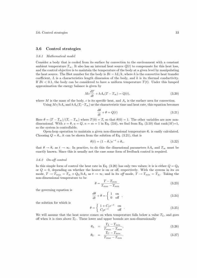
0 1 2 3 4 50
0.1
0.2
0.3
0.4
0.5
0.6
0.7
0.8
0.9
1
θU
θL
t
θ
Figure 3.3: Lumped approximation with on-off control.
The result of applying this form of control is an oscillatory temperature that looks like thatin Fig. 3.3, the period and amplitude of which can be chosen using suitable parameters. It can beshown that the on and off time periods are
ton = ln1 − θL
1 − θU, (3.28)
toff = lnθU
θL, (3.29)
respectively. The total period of the oscillation is then
tp = lnθU (1 − θL)
θL(1 − θU ). (3.30)
If we make a small dead-band assumption, we can write
θL = θr − δ, (3.31)
θU = θr + δ, (3.32)
where δ ≪ 1. A Taylor-series expansion gives
tp = 2 δ
(1
θr+
1
1 − θr
)+ . . . (3.33)
The period is thus proportional to the width of the dead band. The frequency of the oscillationincreases as its amplitude decreases.
3.6.3 PID control
The error e = θr − θ and control input u = Q can be used in Eq. (3.5), so that the derivative of Eq.(3.21) gives
(Kd + 1)d2θ
dt2+ (Kp + 1)
dθ
dt+Kiθ = Kiθr, (3.34)
3.6. Control strategies 35
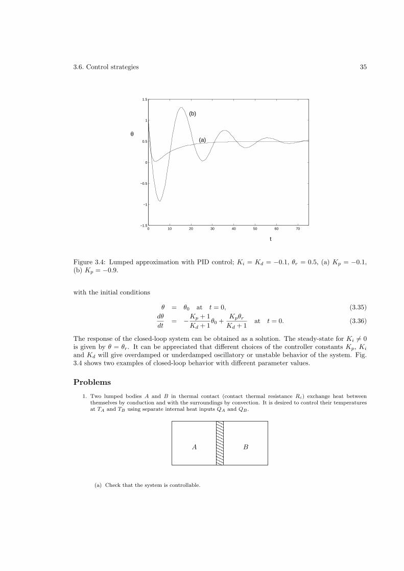
0 10 20 30 40 50 60 70−1.5
−1
−0.5
0
0.5
1
1.5
θ
t
(a)
(b)
Figure 3.4: Lumped approximation with PID control; Ki = Kd = −0.1, θr = 0.5, (a) Kp = −0.1,(b) Kp = −0.9.
with the initial conditions
θ = θ0 at t = 0, (3.35)
dθ
dt= −Kp + 1
Kd + 1θ0 +
Kpθr
Kd + 1at t = 0. (3.36)
The response of the closed-loop system can be obtained as a solution. The steady-state for Ki 6= 0is given by θ = θr. It can be appreciated that different choices of the controller constants Kp, Ki
and Kd will give overdamped or underdamped oscillatory or unstable behavior of the system. Fig.3.4 shows two examples of closed-loop behavior with different parameter values.
Problems
1. Two lumped bodies A and B in thermal contact (contact thermal resistance Rc) exchange heat betweenthemselves by conduction and with the surroundings by convection. It is desired to control their temperaturesat TA and TB using separate internal heat inputs QA and QB .
A B
(a) Check that the system is controllable.
3.6. Control strategies 36
(b) Set up a PID controller where its constants are matrices. Determine the condition for linear stability ofthe control system. Show that the case of two independent bodies is recovered as Rc → ∞.
(c) Calculate and plot TA(t) and TB(t) for chosen values of the controller constants.
2. Apply an on-off controller to the previous problem. Plot TA(t) and TB(t) for selected values of the parameters.Check for phase synchronization.
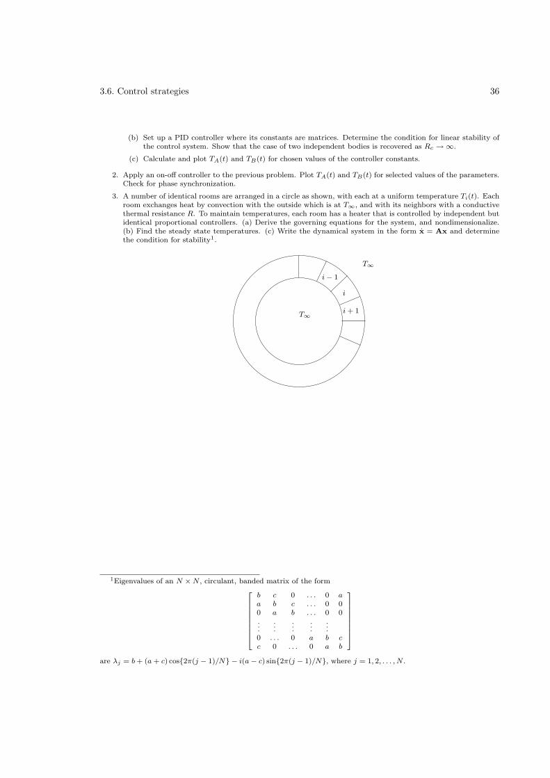
3. A number of identical rooms are arranged in a circle as shown, with each at a uniform temperature Ti(t). Eachroom exchanges heat by convection with the outside which is at T∞, and with its neighbors with a conductivethermal resistance R. To maintain temperatures, each room has a heater that is controlled by independent butidentical proportional controllers. (a) Derive the governing equations for the system, and nondimensionalize.(b) Find the steady state temperatures. (c) Write the dynamical system in the form x = Ax and determinethe condition for stability1.
i − 1
i
i + 1
T∞
T∞
1Eigenvalues of an N × N , circulant, banded matrix of the form
2
6
6
6
6
6
6
6
4
b c 0 . . . 0 aa b c . . . 0 00 a b . . . 0 0...
.
.
....
.
.
....
0 . . . 0 a b cc 0 . . . 0 a b
3
7
7
7
7
7
7
7
5
are λj = b + (a + c) cos2π(j − 1)/N − i(a − c) sin2π(j − 1)/N, where j = 1, 2, . . . , N .

Part III
One spatial dimension
37
Chapter 4
Conduction
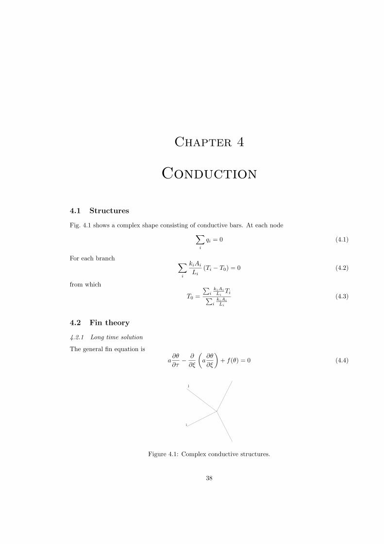
4.1 Structures
Fig. 4.1 shows a complex shape consisting of conductive bars. At each node
∑
i
qi = 0 (4.1)
For each branch ∑
i
kiAi
Li(Ti − T0) = 0 (4.2)
from which
T0 =
∑i
kiAi
LiTi∑
ikiAi
Li
(4.3)
4.2 Fin theory
4.2.1 Long time solution
The general fin equation is
a∂θ
∂τ− ∂
∂ξ
(a∂θ
∂ξ
)+ f(θ) = 0 (4.4)
i
j
Figure 4.1: Complex conductive structures.
38
4.2. Fin theory 39
where f(θ) includes heat transfer from the sides due to convection and radiation. The boundaryconditions are either Dirichlet or Neumannn type at ξ = 0 and ξ = 1. The steady state is determinedfrom
− d
dξ
(adθ
dξ
)+ f(θ) = 0 (4.5)
with the same boundary conditions. Substituting θ = θ+ θ′ in equation (4.4) and subtracting (4.5),we have
a∂θ′
∂τ− ∂
∂ξ
(a∂θ′
∂ξ
)+[f(θ + θ′) − f(θ)
]= 0 (4.6)
where θ′ is the perturbation from the steady state. The boundary conditions for θ′ are homogeneous.Multiplying by θ′ and integrating from ξ = 0 to ξ = 1, we have
dE
dτ= I1 + I2 (4.7)
where
E =1
2
∫ 1
0
a(θ′)2 dξ (4.8)
I1 =
∫ 1
0
θ′∂
∂ξ
(a∂θ′
∂ξ
)dξ (4.9)
I2 = −∫ 1
0
θ′[f(θ + θ′) − f(θ)
]dξ (4.10)
Integrating by parts we can show that
I1 = θ′a∂θ′
∂ξ
∣∣∣∣∣
1
0
−∫ 1
0
a
(dθ′
dξ
)2
dξ (4.11)
= −∫ 1
0
a
(dθ′
dξ
)2
dξ (4.12)
since the first term on the right side of equation (4.11) is zero due to boundary conditions. Thus weknow from the above that I1 is nonpositive and from equation (4.8) that E is nonnegative. If wealso assume that
I2 ≤ 0 (4.13)
then equation (4.7) tells us that E must decrease with time until reaching zero. Thus the steadystate is globally stable. Condition (4.13) holds if [θ′ and f(θ + θ′) − f(θ)] are of the same sign orboth zero; this is a consequence of the Second Law of Thermodynamics.
4.2.2 Shape optimization of convective fin
Consider a rectangular fin of length L and thickness δ as shown in Fig. 4.2. The dimensional equationis
d2T
dx2−m2(T − T∞) = 0 (4.14)
where
m =
(2h
ksδ
)1/2
(4.15)
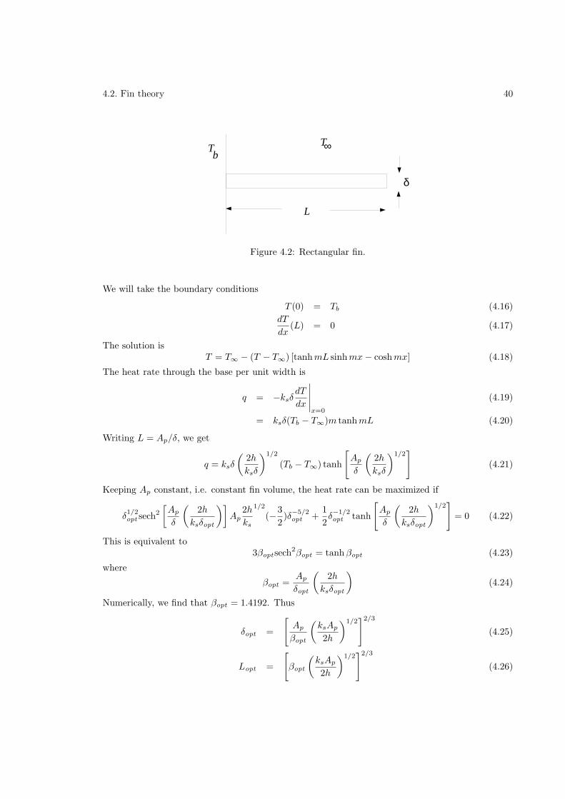
4.2. Fin theory 40
L
Tb
∞T
δ
Figure 4.2: Rectangular fin.
We will take the boundary conditions
T (0) = Tb (4.16)
dT
dx(L) = 0 (4.17)
The solution isT = T∞ − (T − T∞) [tanhmL sinhmx− coshmx] (4.18)
The heat rate through the base per unit width is
q = −ksδdT
dx
∣∣∣∣∣x=0
(4.19)
= ksδ(Tb − T∞)m tanhmL (4.20)
Writing L = Ap/δ, we get
q = ksδ
(2h
ksδ
)1/2
(Tb − T∞) tanh
[Ap
δ
(2h
ksδ
)1/2]
(4.21)
Keeping Ap constant, i.e. constant fin volume, the heat rate can be maximized if
δ1/2opt sech
2
[Ap
δ
(2h
ksδopt
)]Ap
2h
ks
1/2
(−3
2)δ
−5/2opt +
1
2δ−1/2opt tanh
[Ap
δ
(2h
ksδopt
)1/2]
= 0 (4.22)
This is equivalent to3βoptsech
2βopt = tanhβopt (4.23)
where
βopt =Ap
δopt
(2h
ksδopt
)(4.24)
Numerically, we find that βopt = 1.4192. Thus
δopt =
[Ap
βopt
(ksAp
2h
)1/2]2/3
(4.25)
Lopt =
[βopt
(ksAp
2h
)1/2]2/3
(4.26)
4.3. Fin structure 41
4.3 Fin structure
Consider now Fig. 4.1 with convection.
4.4 Fin with convection and radiation
Steady state solutionsEquation (4.4) reduces to
− d
dξ
(adθ
dξ
)+m2pθ + ǫp
[(θ + β)4 − β4
]= 0 (4.27)
Uniform cross section
For this case a = p = 1, so that
−d2θ
dξ2+m2θ + ǫ
[(θ + β)4 − β4
]= 0 (4.28)
Convective
With only convective heat transfer, we have
−d2θ
dξ2+m2θ = 0 (4.29)
the solution to whiich isθ = C1 sinhmξ + C2 coshmξ (4.30)
the constants are determined from the boundary conditions. For example, if
θ(0) = 1 (4.31)
dθ
dξ(1) = 0 (4.32)
we getθ = − tanhm sinhmξ + coshmξ (4.33)
Example 4.1If
T (0) = T0 (4.34)
T (L) = T1 (4.35)
then show that
T (x) =
"
T1 − T0 cosh
L
r
hP
kA
!# sinh
„
xq
hPkA
«
sinh
„
Lq
hPkA
« + T0 cosh
x
r
hP
kA
!
(4.36)
4.4. Fin with convection and radiation 42
Radiative
The fin equation is
−d2θ
dξ2+ ǫ[(θ + β)4 − β4
]= 0 (4.37)
Letφ = θ + β (4.38)
so that
−d2φ
dξ2+ ǫφ4 = −ǫβ4 (4.39)
As an example, we will find a perturbation solution with the boundary conditions
φ(0) = 1 + β (4.40)
dφ
dξ(1) = 0 (4.41)
We writeφ = φ0 + ǫφ1 + ǫ2φ2 + . . . (4.42)
The lowest order equation is
dφ0
dξ2= 0, φ0(0) = 1 + β,
dφ0
dξ(1) = 0 (4.43)
which givesφ0 = 1 + β (4.44)
To the next orderdφ1
dξ2= φ4
0 − β4, φ1(0) = 0,dφ1
dξ(1) = 0 (4.45)
with the solution
φ1 = [(1 + β)4 − β4]ξ2
2− [(1 + β)4 − β4]ξ (4.46)
The complete solution is
φ = (1 + β) + ǫ
[(1 + β)4 − β4]
ξ2
2− [(1 + β)4 − β4]ξ
+ . . . (4.47)
so that
θ = 1 + ǫ
[(1 + β)4 − β4]
ξ2
2− [(1 + β)4 − β4]ξ
+ . . . (4.48)
Convective and radiative
(4.49)
4.5. Perturbations of one-dimensional conduction 43
4.4.1 Annular fin
Example 4.2Show that under suitable conditions, the temperature distribution in a two-dimensional rectangle tends
to that given by a one-dimensional approximation.
4.5 Perturbations of one-dimensional conduction
4.5.1 Temperature-dependent conductivity
[13]The governing equation is
d
dx
(k(T )
dT
dx
)− Ph
A(T − T∞) = 0 (4.50)
with the boundary conditions
T (0) = Tb (4.51)
dT
dx(L) = 0 (4.52)
we use the dimensionless variables
θ =T − T∞Tb − T∞
(4.53)
ξ =x
L(4.54)
Consider the special case of a linear variation of conductivity
k(T ) = k0
(1 + ǫ
T − T∞Tb − T∞
)(4.55)
so that
(1 + ǫθ)d2θ
dξ2+ ǫ
(dθ
dξ
)2
−m2θ = 0 (4.56)
θ(0) = 1 (4.57)
dθ
dξ(L) = 0 (4.58)
where
m2 =PhL2
Ak0(Tb − T∞)(4.59)
Introduceθ(ξ) = θ0(ξ) + ǫθ1(ξ) + ǫθ2(ξ) + . . . (4.60)
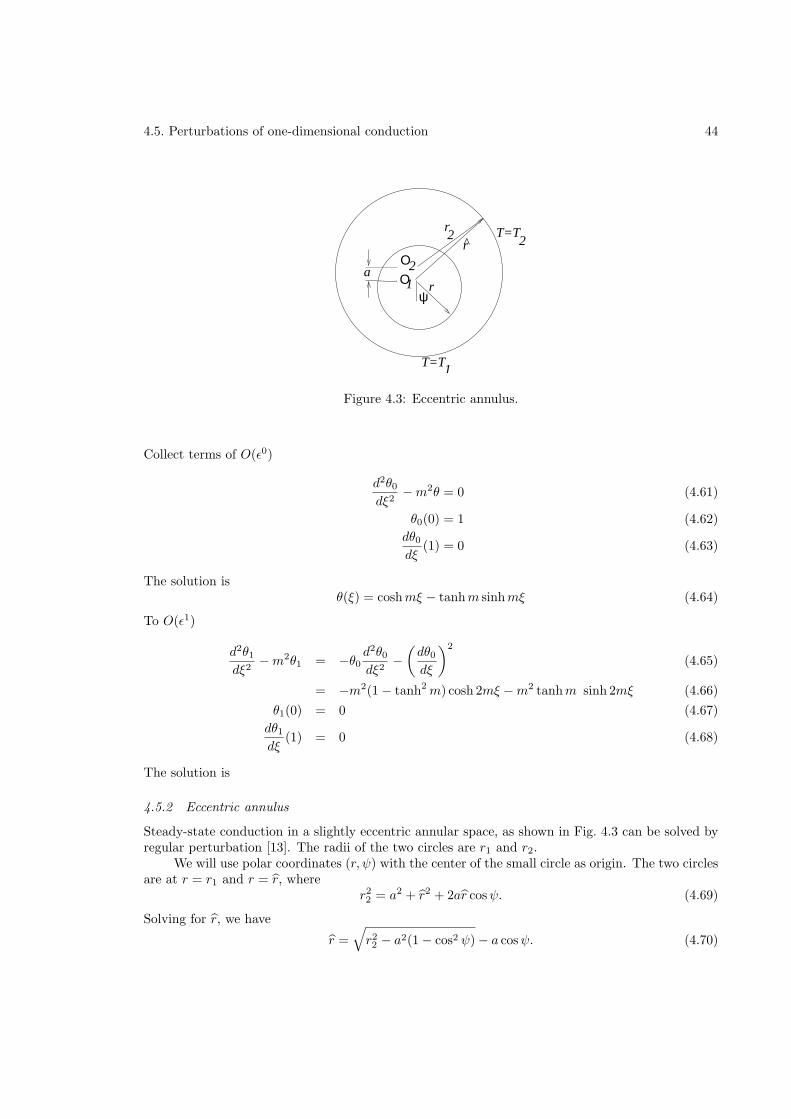
4.5. Perturbations of one-dimensional conduction 44
r
T=T
T=T
1
22r
r
ψ
2ΟΟ1
a
Figure 4.3: Eccentric annulus.
Collect terms of O(ǫ0)
d2θ0dξ2
−m2θ = 0 (4.61)
θ0(0) = 1 (4.62)
dθ0dξ
(1) = 0 (4.63)
The solution isθ(ξ) = coshmξ − tanhm sinhmξ (4.64)
To O(ǫ1)
d2θ1dξ2
−m2θ1 = −θ0d2θ0dξ2
−(dθ0dξ
)2
(4.65)
= −m2(1 − tanh2m) cosh 2mξ −m2 tanhm sinh 2mξ (4.66)
θ1(0) = 0 (4.67)
dθ1dξ
(1) = 0 (4.68)
The solution is
4.5.2 Eccentric annulus
Steady-state conduction in a slightly eccentric annular space, as shown in Fig. 4.3 can be solved byregular perturbation [13]. The radii of the two circles are r1 and r2.
We will use polar coordinates (r, ψ) with the center of the small circle as origin. The two circlesare at r = r1 and r = r, where
r22 = a2 + r2 + 2ar cosψ. (4.69)
Solving for r, we have
r =√r22 − a2(1 − cos2 ψ) − a cosψ. (4.70)
4.5. Perturbations of one-dimensional conduction 45
In the quadratic solution, the positive sign corresponding to the geometry shown in the figure hasbeen kept.
The governing equation for the temperature is
(∂2
∂r2+
1
r
∂
∂r+
1
r2∂2
∂ψ2
)T (r, ψ) = 0. (4.71)
The boundary conditions are
T (r1, ψ) = T1, (4.72)
T (r, ψ) = T2. (4.73)
With the variables
θ =T − T2
T1 − T2. (4.74)
R =r − r1r2 − r1
. (4.75)
d =r1
r2 − r1. (4.76)
ǫ =a
r2 − r1, (4.77)
we get (∂2
∂R2+
1
R+ d
∂
∂R+
1
(R+ d)2∂2
∂ψ2
)θ(R,ψ) = 0, (4.78)
and
θ(0, ψ) = 1, (4.79)
θ(R, ψ) = 0, (4.80)
where
R(ψ) =r − r1r2 − r1
=√
(1 + d)2 − ǫ2(1 − cos2 ψ) − ǫ cosψ − d, (4.81)
The perturbation expansion is
θ(R,ψ) = θ0(R,ψ) + ǫθ1(R,ψ) + ǫ2θ2(R,ψ) + . . . . (4.82)
Substituting in the equations, we get
(∂2
∂R2+
1
R+ d
∂
∂R+
1
(R+ d)2∂2
∂ψ2
)(θ0 + ǫθ1 + ǫ2θ2 + . . .
)= 0, (4.83)
R(ψ) = 1 − ǫ cosψ − ǫ2
2(1 − cos2 ψ) + . . . , (4.84)
θ0(0, ψ) + ǫθ1(0, ψ) + ǫ2θ2(0, ψ) + . . . = 1, (4.85)
θ0(R, ψ) + ǫθ1(R, ψ) + ǫ2θ2(R, ψ) + . . . = 0. (4.86)
4.6. Transient conduction 46
Using Eq. (4.84), (4.86) can be further expanded in a Taylor series around R = 1 to give
θ0(1, ψ) + ǫ
(θ1(1, ψ) − cosψ
dθ0dR
(1, ψ)
)+ . . . = 0. (4.87)
Collecting terms to order O(ǫ0), we get
(∂2
∂R2+
1
R+ d
∂
∂R+
1
(R+ d)2∂2
∂ψ2
)θ0 = 0, (4.88)
θ0(0, ψ) = 1, (4.89)
θ0(1, ψ) = 0, (4.90)
which has the solution
θ0(R,ψ) = 1 − ln(1 +R/h)
ln(1 + 1/h). (4.91)
To order O(ǫ1)
(∂2
∂R2+
1
R+ d
∂
∂R+
1
(R+ d)2∂2
∂ψ2
)θ1 = 0, (4.92)
θ1(0, ψ) = 0, (4.93)
θ1(1, ψ) = cosψdθ0dR
(1, ψ), (4.94)
=cosψ
(1 + h) ln(1 + 1/h). (4.95)
The solution is
θ1(R,ψ) = ± R cosψ
(1 + 2h) ln(1 + 1/h)
R− 2h
R+ h. (4.96)
4.6 Transient conduction
Let us propose a similarity solution of the transient conduction equation
∂2T
∂x2− 1
κ
∂T
∂t= 0 (4.97)
as
T = A erf
(x
2√κt
)(4.98)
Taking derivatives we find
∂T
∂x= A
1√πκt
exp
(− x2
4κt
)(4.99)
∂2T
∂x2= −A x
2√πκ3t3
exp
(− x2
4κt
)(4.100)
∂T
∂t= −A x
2√πκt3
exp
(− x2
4κt
)(4.101)
so that substitution verifies that equation (4.98) is a solution to equation (4.97).
4.7. Linear diffusion 47
4.7 Linear diffusion
Let T = T (x, t) and∂T
∂t= α
∂2T
∂x2(4.102)
in 0 ≤ x ≤ L, with the boundary and initial conditions T (0, t) = T1, T (L, t) = T2, and T (x, 0) =f(x). The steady state solution is
T (x) = T1 +T2 − T1
Lx. (4.103)
WithT ′(x, t) = T − T (4.104)
we have the same equation∂T ′
∂t= α
∂2T ′
∂x2(4.105)
but with the conditions: T ′(0, t) = 0, T ′(L, t) = 0, and T ′(x, 0) = f(x) − T .Following the methodology outlined in Section A.6.1, we consider the eigenvalue problem
d2φ
dx2= λφ (4.106)
with φ(0) = φ(L) = 0. The operator is self-adjoint. Its eigenvalues are
λi = − i2π2
L2, (4.107)
and its orthonormal eigenfunctions are
φi(x) =
√2
Lsin
iπx
L. (4.108)
Thus we let
θ(x, t) =
∞∑
i=1
ai(t)φi(x), (4.109)
so thatdaj
dt= −α
(jπ
L
)2
aj , (4.110)
with the solution
aj = Cj exp
−α
(jπ
L
)2
t
. (4.111)
Thus
T ′(x, t) =
∞∑
i=1
Cj exp
−α
(jπ
L
)2
t
√2
Lsin
iπx
L. (4.112)
The solution shows that T ′ → 0, as t→ ∞. Thus θ = 0 is a stable solution of the problem. Itmust be noted that there has been no need to linearize, since Eq. (4.105) was already linear.
4.8. Nonlinear diffusion 48
4.8 Nonlinear diffusion
The following diffusion problem with heat generation is considered in [81]
∂T
∂t= ǫ
∂2T
∂x2+ f(T ), (4.113)
with −∞ < x <∞, t ≥ 0, and ǫ≪ 1. The initial condition is taken to be
T (x, 0) = g(x) (4.114)
=1
1 + eλx. (4.115)
Consider two time scales, a fast, short one t1 = t, and a slow, long scale t2 = ǫt. Thus
∂
∂t=
∂
∂t1+ ǫ
∂
∂t2. (4.116)
Assuming an asymptotic expansion of the type
T = T0(x, t1, t2) + ǫT1(x, t1, t2) + . . . (4.117)
we have a Taylor series expansion
f(T ) = f(T0) + ǫf ′(T0) + . . . (4.118)
Substituting and collecting terms of O(ǫ0), we get
∂T0
∂t1= f(T0), (4.119)
with the solution ∫ T0
1/2
dr
f(r)= t1 + θ(x, t2). (4.120)
The lower limit of the integral is simply a convenient value at which g(x) = 0.5. Applying the initialcondition gives
θ =
∫ g(x)
1/2
dr
f(r). (4.121)
The terms of O(ǫ) are∂T1
∂t1= f ′(T0)T1 +
∂2T0
∂x2− ∂T0
∂t2(4.122)
Differentiating Eq. 4.120 with respect to x gives
∂T0
∂x= f(T0)
∂θ
∂x, (4.123)
so that
∂2T0
∂x2= f ′(T0)
∂T0
∂x
∂θ
∂x+ f(T0)
∂2θ
∂x2
= f ′(T0)f(T0)
(∂θ
∂x
)2
+ f(T0)∂@2θ
∂x2(4.124)
4.8. Nonlinear diffusion 49
Also, differentiating with respect to t2 gives
∂T0
∂t2= f(T0)
∂θ
∂t2(4.125)
Substituting in Eq. 4.122,
∂T1
∂t1= f ′(T0)T1 + f(T0)
[∂2θ
∂x2− ∂θ
∂t2+ f ′(T0)
(∂θ
∂x
)2]. (4.126)
Since
∂
∂t1ln f(T0) =
f ′(T0)
f(T0)
∂T0
∂t1(4.127)
= f ′(T0) (4.128)
we have∂T1
∂t1= f ′(T0)T1 + f(T0)
[∂2θ
∂x2− ∂θ
∂t2+
∂
∂t1ln f(T0)
]. (4.129)
The solution is
T1 =
[A(x, t2) + t1
(∂2θ
∂x2− ∂θ
∂t2+
(∂θ
∂x
)2
ln f(T0)
)]f(T0) (4.130)
which can be checked by differentiation since
∂T1
∂t1=
[∂2θ
∂x2− ∂θ
∂t2+ f ′(T0)
(∂θ
∂x
)2]f(T0) (4.131)
+
[A+ t1
(∂2θ
∂x2− ∂θ
∂t2
)+
(∂θ
∂x
)2
ln f(T0)
]f ′(T0)
∂T0
∂t1(4.132)
=
[∂2θ
∂x2− ∂θ
∂t2+ f ′(T0)
(∂θ
∂x
)2]f(T0) + T1f
′(T0). (4.133)
where Eq. 4.119 has been used.To suppress the secular term in Eq. 4.130, we take
∂2θ
∂x2− ∂θ
∂t2+ κ(x, t1)
(∂θ
∂x
)2
= 0. (4.134)
where κ = f ′(T0). Letw(x, t2) = eκθ, (4.135)
so that its derivatives are
∂w
∂x= κeκθ ∂θ
∂x(4.136)
∂2w
∂x2= κ2eκθ
(∂θ
∂x
)2
+ κeκθ ∂2θ
∂x2(4.137)
∂w
∂t2= κeκθ ∂θ
∂t2(4.138)
4.8. Nonlinear diffusion 50
We find that
∂2w
∂x2− ∂w
∂t2= κeκθ
[∂2θ
∂x2− ∂θ
∂t2+ κ
(∂θ
∂x
)2]
(4.139)
= 0. (4.140)
The solution is
w =1√π
∫∞
∞
R(x+ 2r√t2)e
−r2
dr, (4.141)
where R(x) = w(x, 0). This can be confirmed by finding the derivatives
∂2w
∂x2=
1√π
∫∞
∞
R′′(x+ 2r√t2)e
−r2
dr (4.142)
∂w
∂t2=
1√π
∫∞
∞
R′(x+ 2r√t2)
r√t2e−r2
dr
= − 1
2√π
[R′(x+ 2r
√t2)
∣∣∣∣∣
∞
∞
−∫
∞
∞
R′′(x+ 2r√t2)2
√t2e
−r2
dr
](4.143)
=1√π
∫∞
∞
R′′(x+ 2r√t2)e
−r2
dr (4.144)
and substituting. Also,
R(x) = exp [κθ(x, 0)] (4.145)
= exp
[κ
∫ g(x)
1/2
dr
f(r)
](4.146)
so that the final (implicit) solution is
∫ T0
1/2
dr
f(r)= t1 +
1
κln
[1√π
∫∞
∞
R(x+ 2r√t2)e
−r2
dr
](4.147)
Fisher’s equation: As an example, we take f(T ) = T (1 − T ), so that the integral in Eq. 4.120is ∫ T0
1/2
dr
r(1 − r)= ln
T0
T0 − 1(4.148)
Substituting in the equation, we get
T0 =1
1 + e−(t1+θ)(4.149)
=w
w + e−t1(4.150)
Thus
w =T0e
−t1
1 − T0(4.151)
and from Eq. 4.115,
R(x) = w(x, 0) (4.152)
= e−λx (4.153)
4.9. Stability by energy method 51
Substituting in Eq. 4.141 and integrating,
w = exp(−λx+ λ2t2
)(4.154)
so that
T0 =1
1 + exp [x− t(1 + λ2ǫ)/λ](4.155)
This is a wave that travels with a phase speed of (1 + λ2ǫ)/λ.
4.9 Stability by energy method
4.9.1 Linear
As an example consider the same problem as in Section 4.7. The deviation from the steady state isgoverned by
∂T ′
∂t= α
∂2T ′
∂x2(4.156)
with T ′(0, t) = 0, T ′(L, t) = 0.Define
E(t) =1
2
∫ L
0
T ′2 dx (4.157)
so that E ≥ 0. Also
dE
dt=
∫ L
0
T ′∂T ′
∂tdx
= α
∫ L
0
T ′∂2T ′
∂x2dx
= α
∫ L
0
T ′∂T ′
∂x
∣∣∣∣∣
L
0
−∫ L
0
(∂T ′
∂x
)2
dx
= −α∫ L
0
(∂T ′
∂x
)2
dx (4.158)
so thatdE
dt≤ 0. (4.159)
Thus E → 0 as t→ ∞ whatever the initial conditions.
4.9.2 Nonlinear
Let us now re-do the problem for a bar with temperature-dependent conductivity. Thus
∂T
∂t=
∂
∂x
k(T )
∂T
∂x
, (4.160)
with T (0, t) = T1 and T (L, t) = T2. The steady state, T (x), is governed by
d
dx
k(T )
dT
dx
= 0. (4.161)
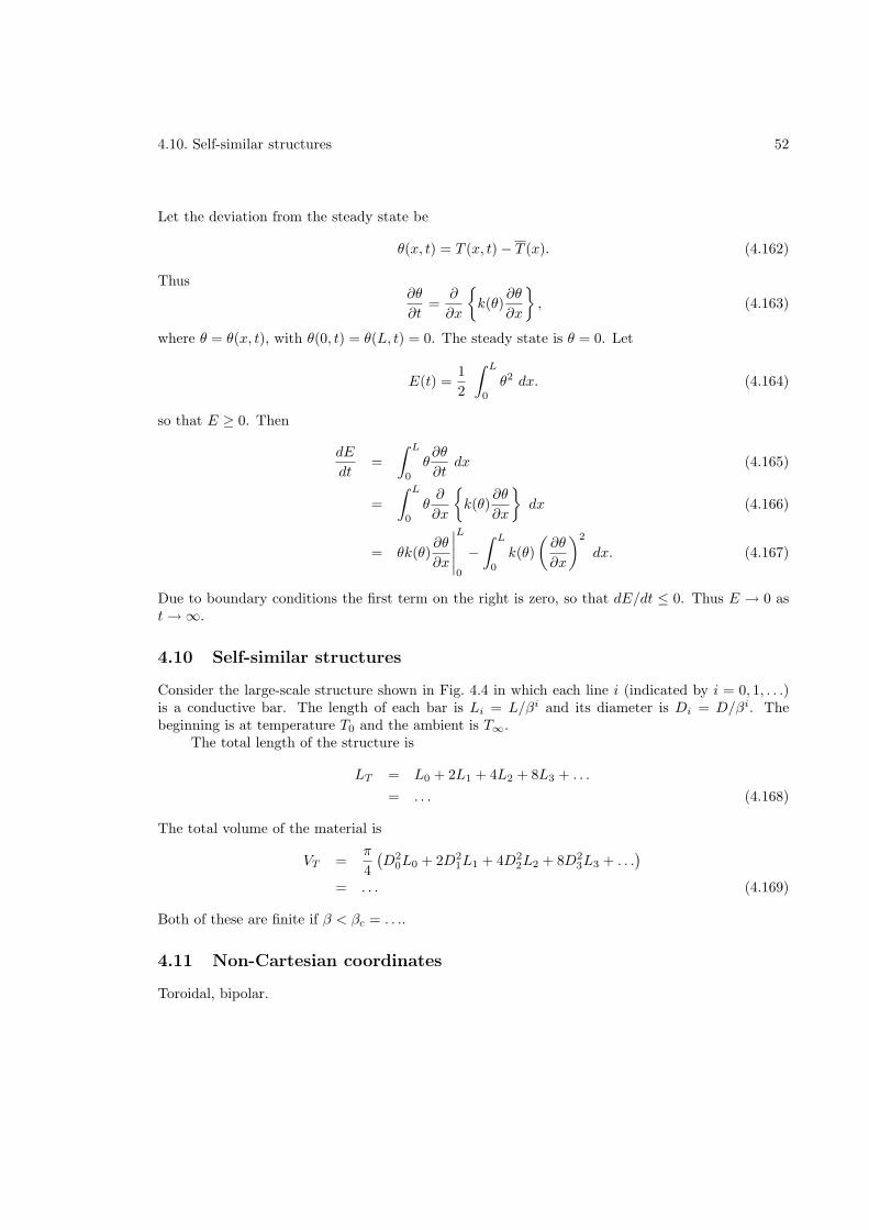
4.10. Self-similar structures 52
Let the deviation from the steady state be
θ(x, t) = T (x, t) − T (x). (4.162)
Thus∂θ
∂t=
∂
∂x
k(θ)
∂θ
∂x
, (4.163)
where θ = θ(x, t), with θ(0, t) = θ(L, t) = 0. The steady state is θ = 0. Let
E(t) =1
2
∫ L
0
θ2 dx. (4.164)
so that E ≥ 0. Then
dE
dt=
∫ L
0
θ∂θ
∂tdx (4.165)
=
∫ L
0
θ∂
∂x
k(θ)
∂θ
∂x
dx (4.166)
= θk(θ)∂θ
∂x
∣∣∣∣∣
L
0
−∫ L
0
k(θ)
(∂θ
∂x
)2
dx. (4.167)
Due to boundary conditions the first term on the right is zero, so that dE/dt ≤ 0. Thus E → 0 ast→ ∞.
4.10 Self-similar structures
Consider the large-scale structure shown in Fig. 4.4 in which each line i (indicated by i = 0, 1, . . .)is a conductive bar. The length of each bar is Li = L/βi and its diameter is Di = D/βi. Thebeginning is at temperature T0 and the ambient is T∞.
The total length of the structure is
LT = L0 + 2L1 + 4L2 + 8L3 + . . .
= . . . (4.168)
The total volume of the material is
VT =π
4
(D2
0L0 + 2D21L1 + 4D2
2L2 + 8D23L3 + . . .
)
= . . . (4.169)
Both of these are finite if β < βc = . . ..
4.11 Non-Cartesian coordinates
Toroidal, bipolar.
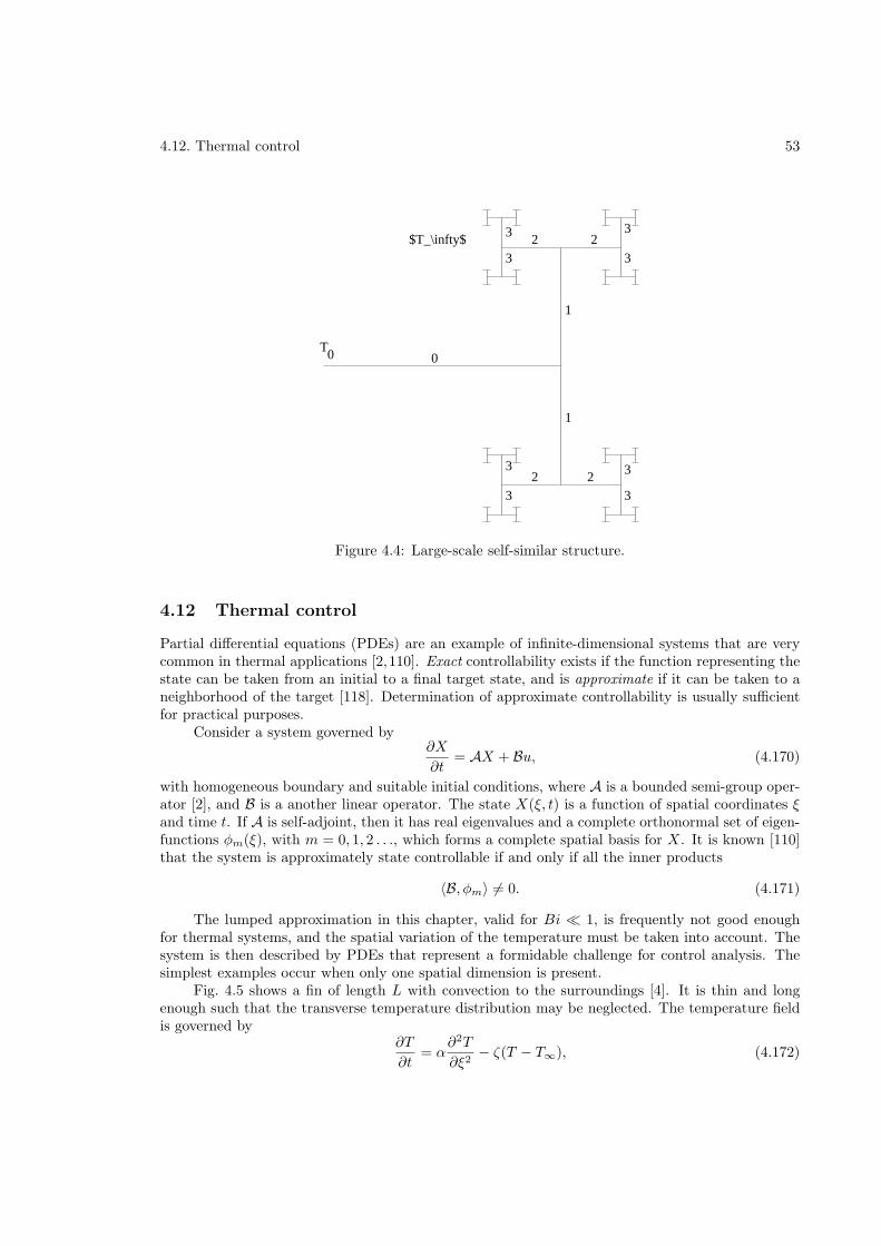
4.12. Thermal control 53
$T_\infty$
1
1
22
2 23
3
3
33
0T
3
3
3
0
Figure 4.4: Large-scale self-similar structure.
4.12 Thermal control
Partial differential equations (PDEs) are an example of infinite-dimensional systems that are verycommon in thermal applications [2,110]. Exact controllability exists if the function representing thestate can be taken from an initial to a final target state, and is approximate if it can be taken to aneighborhood of the target [118]. Determination of approximate controllability is usually sufficientfor practical purposes.
Consider a system governed by∂X
∂t= AX + Bu, (4.170)
with homogeneous boundary and suitable initial conditions, where A is a bounded semi-group oper-ator [2], and B is a another linear operator. The state X(ξ, t) is a function of spatial coordinates ξand time t. If A is self-adjoint, then it has real eigenvalues and a complete orthonormal set of eigen-functions φm(ξ), with m = 0, 1, 2 . . ., which forms a complete spatial basis for X. It is known [110]that the system is approximately state controllable if and only if all the inner products
〈B, φm〉 6= 0. (4.171)
The lumped approximation in this chapter, valid for Bi ≪ 1, is frequently not good enoughfor thermal systems, and the spatial variation of the temperature must be taken into account. Thesystem is then described by PDEs that represent a formidable challenge for control analysis. Thesimplest examples occur when only one spatial dimension is present.
Fig. 4.5 shows a fin of length L with convection to the surroundings [4]. It is thin and longenough such that the transverse temperature distribution may be neglected. The temperature fieldis governed by
∂T
∂t= α
∂2T
∂ξ2− ζ(T − T∞), (4.172)
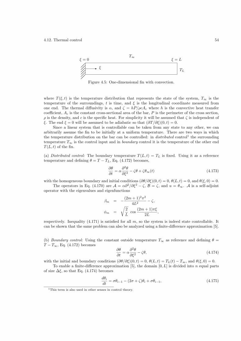
4.12. Thermal control 54
- ξ
ξ = 0 ξ = L
TL
T∞
Figure 4.5: One-dimensional fin with convection.
where T (ξ, t) is the temperature distribution that represents the state of the system, T∞ is thetemperature of the surroundings, t is time, and ξ is the longitudinal coordinate measured fromone end. The thermal diffusivity is α, and ζ = hP/ρcAc where h is the convective heat transfercoefficient, Ac is the constant cross-sectional area of the bar, P is the perimeter of the cross section,ρ is the density, and c is the specific heat. For simplicity it will be assumed that ζ is independent ofξ. The end ξ = 0 will be assumed to be adiabatic so that (∂T/∂ξ)(0, t) = 0.
Since a linear system that is controllable can be taken from any state to any other, we canarbitrarily assume the fin to be initially at a uniform temperature. There are two ways in whichthe temperature distribution on the bar can be controlled: in distributed control1 the surroundingtemperature T∞ is the control input and in boundary control it is the temperature of the other endT (L, t) of the fin.
(a) Distributed control: The boundary temperature T (L, t) = TL is fixed. Using it as a referencetemperature and defining θ = T − TL, Eq. (4.172) becomes,
∂θ
∂t= α
∂2θ
∂ξ2− ζθ + ζθ∞(t) (4.173)
with the homogeneous boundary and initial conditions (∂θ/∂ξ)(0, t) = 0, θ(L, t) = 0, and θ(ξ, 0) = 0.The operators in Eq. (4.170) are A = α∂2/∂ξ2 − ζ, B = ζ, and u = θ∞. A is a self-adjoint
operator with the eigenvalues and eigenfunctions
βm = − (2m+ 1)2π2
4L2− ζ,
φm =
√2
Lcos
(2m+ 1)πξ
2L,
respectively. Inequality (4.171) is satisfied for all m, so the system is indeed state controllable. Itcan be shown that the same problem can also be analyzed using a finite-difference approximation [5].
(b) Boundary control: Using the constant outside temperature T∞ as reference and defining θ =T − T∞, Eq. (4.172) becomes
∂θ
∂t= α
∂2θ
∂ξ2− ζθ, (4.174)
with the initial and boundary conditions (∂θ/∂ξ)(0, t) = 0, θ(L, t) = TL(t) − T∞, and θ(ξ, 0) = 0.To enable a finite-difference approximation [5], the domain [0, L] is divided into n equal parts
of size ∆ξ, so that Eq. (4.174) becomes
dθi
dt= σθi−1 − (2σ + ζ)θi + σθi−1, (4.175)
1This term is also used in other senses in control theory.
4.13. Multiple scales 55
where σ = α/∆ξ2. The nodes are i = 1, 2, . . . , n + 1, where i = 1 is at the left and i = n + 1 atthe right end of the fin in Fig. 4.5. With this Eq. (4.174) can be discretized to take the form of Eq.(3.6), where x is the vector of unknown θi. Thus we find
A =
−(2σ + ζ) 2σ 0 · · · 0
σ −(2σ + ζ) σ...
0. . .
. . .. . .
... σ0 · · · 0 σ −(2σ + ζ)
∈ Rn×n, (4.176)
B = [0, · · · , σ]T ∈ Rn. (4.177)
The boundary conditions have been applied to make A non-singular: at the left end the fin isadiabatic, and at the right end θn+1 is the control input u.
The controllability matrix M is
M =
0 · · · · · · 0 σn
0 · · · 0 σn−1 · · ·...
......
......
0 0 σ3 · · · · · ·0 σ2 −2σ2(2σ + ζ) · · · · · ·σ −σ(2σ + ζ) σ3 + σ(2σ + ζ)2 · · · · · ·
(4.178)
The rank of M is n, indicating that the state of the system is also boundary controllable.
4.13 Multiple scales
Solve
∂T1
∂t= α
∂2(T1 − T2)
∂x2(4.179)
∂T2
∂t= Rα
∂2(T2 − T1)
∂x2(4.180)
where ǫ≪ 1, and with a step change in temperature at one end. Let
t = t0 + ǫt1 (4.181)
Problems
1. From the governing equation for one-dimensional conduction
d
dx
»
k(x, T )dT
dx
–
= 0,
with boundary conditions
T (0) = T +∆T
2,
T (L) = T − ∆T
2.
show that the magnitude of the heat rate is independent of the sign of ∆T if we can write k(x, T ) = A(x) λ(T ).
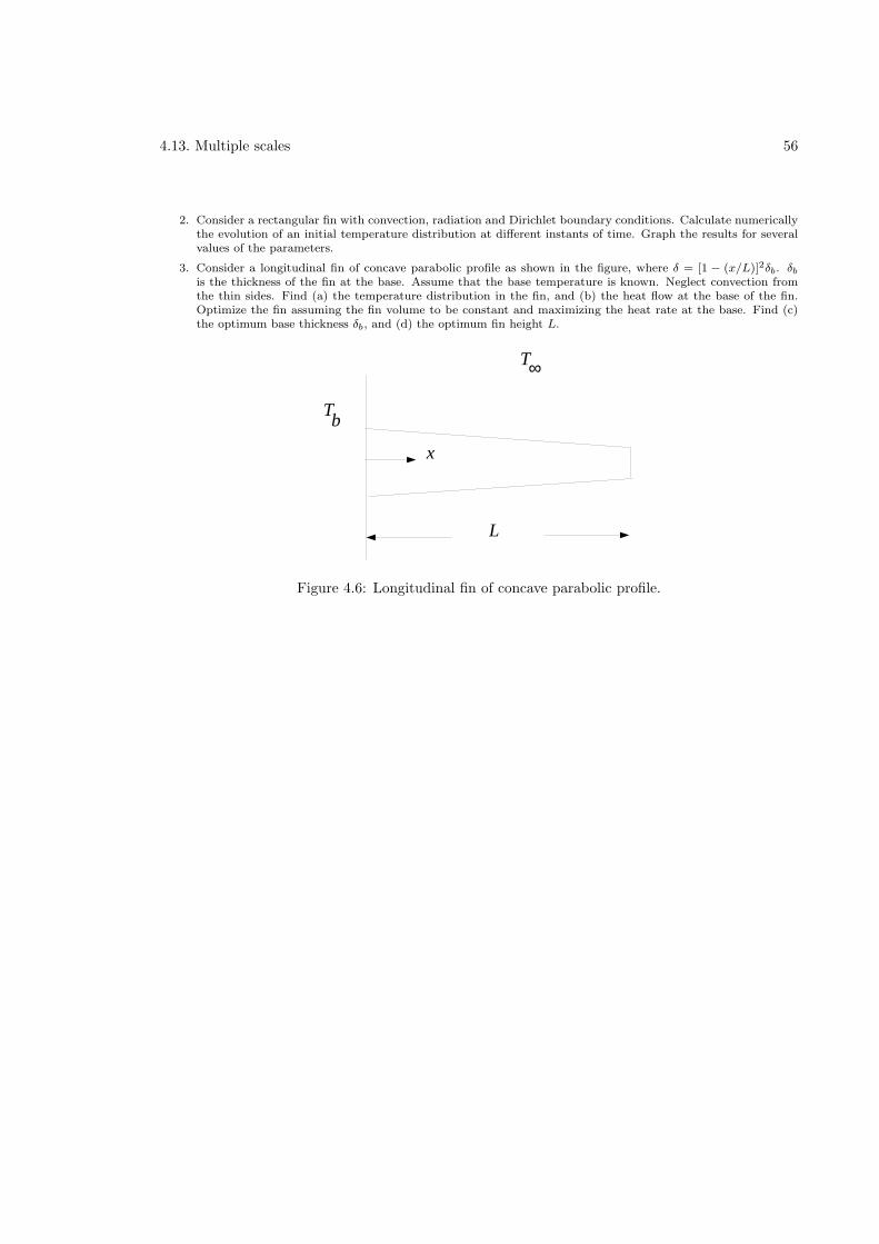
4.13. Multiple scales 56
2. Consider a rectangular fin with convection, radiation and Dirichlet boundary conditions. Calculate numericallythe evolution of an initial temperature distribution at different instants of time. Graph the results for severalvalues of the parameters.
3. Consider a longitudinal fin of concave parabolic profile as shown in the figure, where δ = [1 − (x/L)]2δb. δb
is the thickness of the fin at the base. Assume that the base temperature is known. Neglect convection fromthe thin sides. Find (a) the temperature distribution in the fin, and (b) the heat flow at the base of the fin.Optimize the fin assuming the fin volume to be constant and maximizing the heat rate at the base. Find (c)the optimum base thickness δb, and (d) the optimum fin height L.
T
T
b
∞
x
L
Figure 4.6: Longitudinal fin of concave parabolic profile.
Chapter 5
Forced convection
In this chapter we will considering the heat transfer in pipe flows. We will take a one-dimensional ap-proach and neglect transverse variations in the velocity and temperature. In addition, for simplicity,we will assume that fluid properties are constant and that the area of the pipe is also constant.
5.1 Hydrodynamics
5.1.1 Mass conservation
For a duct of constant cross-sectional area and a fluid of constant density, the mean velocity of thefluid, V , is also constant.
5.1.2 Momentum equation
The forces on an element of length ds, shown in Fig. 5.1, in the positive s direction are: fv, theviscous force and fp, the pressure force. We can write
fv = −τw P ds (5.1)
fp = −A∂p∂sds (5.2)
where τw is the magnitude of the wall shear stress, and p is the pressure in the fluid. Since the massof the element is ρA ds, we can write the momentum equation as
ρA dsdV
dt= fv + fp (5.3)
from which we getdV
dt+τwP
ρA= −1
ρ
∂p
∂s(5.4)
Integrating over the length L of a pipe, we have
dV
dt+
4τwρD
=p1 − p2
ρL(5.5)
where p1 and p2 are the pressures at the inlet and outlet respectively, and the hydraulic diameter isdefined by D = 4A/P .
57
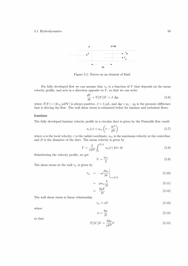
5.1. Hydrodynamics 58
ds
s
p p+dp
f
f
p
v
Figure 5.1: Forces on an element of fluid.
For fully developed flow we can assume that τw is a function of V that depends on the meanvelocity profile, and acts in a direction opposite to V , so that we can write
dV
dt+ T (|V |)V = β ∆p (5.6)
where T (V ) = |4τw/ρDV | is always positive, β = 1/ρL, and ∆p = p1 − p2 is the pressure differencethat is driving the flow. The wall shear stress is estimated below for laminar and turbulent flows.
Laminar
The fully developed laminar velocity profile in a circular duct is given by the Poiseuille flow result
ux(r) = um
(1 − 4r2
D2
)(5.7)
where u is the local velocity, r is the radial coordinate, um is the maximum velocity at the centerline,and D is the diameter of the duct. The mean velocity is given by
V =4
πD2
∫ D/2
0
ux(r) 2πr dr (5.8)
Substituting the velocity profile, we get
V =um
2(5.9)
The shear stress at the wall τw is given by
τw = −µ∂ux
∂r
∣∣∣∣∣r=D/2
(5.10)
= µum4
D(5.11)
=8µV
D(5.12)
The wall shear stress is linear relationship
τw = αV (5.13)
where
α =8µ
D(5.14)
so that
T (|V |)V =32µ
ρD2V (5.15)
5.1. Hydrodynamics 59
Turbulent
For turbulent flow the expression for shear stress at the wall of a duct that is usually used is
τw =f
4
(1
2ρV 2
)(5.16)
so that
T (V ) =f
2D|V |V. (5.17)
Here f is the Darcy-Weisbach friction factor1. The friction factor is also a fucntion of |V |, and maybe calculated from the Blasius equation for smooth pipes
f =0.3164
Re1/4(5.18)
where the Reynolds number is Re = |V |D/ν, or the Colebrook equation for rough pipes
1
f1/2= −2.0 log
(e/Dh
3.7+
2.51
Re f1/2
)(5.19)
where e is the roughness at the wall, or similar expressions.In the flow in a length of duct, L, without acceleration, the pressure drop is given by
∆p A = τwPL (5.20)
where A is the cross-sectional area, and P is the inner perimeter. Thus
∆p = f
(L
4A/P
) (1
2ρV 2
)(5.21)
= f
(L
D
) (1
2ρ|V |V
)(5.22)
Example 5.1Consider a long, thin pipe with pressures p1 and p2 ate either end. For t ≤ 0, p1 − p2 = 0 and there is no
flow. For t > 0, p1 − p2 is a nonzero constant. Find the resulting time-dependent flow. Make the assumptionthat the axial velocity is only a function of radial position and time.
5.1.3 Long time behavior
Consider the flow in a single duct of finite length with a constant driving pressure drop. Thegoverning equation for the flow velocity is equation (5.6). The flow velocity in the steady state is asolution of
T (V )V = β ∆p (5.23)
1Sometimes, confusingly, the Fanning friction factor, which is one-fourth the Darcy-Weisbach value, is used in theliterature.
5.2. Energy equation 60
where ∆p and V are both of the same sign, say nonnegative. We can show that under certainconditions the steady state is globally stable. Writing V = V + V ′, equation (5.6) becomes
dV ′
dt+ T (V + V ′)(V + V ′) = β ∆p (5.24)
Subtracting equation (5.23), we get
dV ′
dt= −T (V + V ′)(V + V ′) + T (V )(V ) (5.25)
Defining
E =1
2V ′2 (5.26)
so that E ≥ 0, we find that
dE
dt= V ′
dV ′
dt(5.27)
= −V ′[T (V + V ′)(V + V ′) − T (V )V
](5.28)
= −V ′V[T (V + V ′) − T (V )
]− V ′2T (V + V ′) (5.29)
If we assume that T (V ) is a non-decreasing function of V , we see that
V ′V[T (V + V ′) − T (V )
]≥ 0 (5.30)
regardless of the sign of either V ′ or V , so that
dE
dt≤ 0 (5.31)
Thus, E(V ) is a Lyapunov function, and V = V is globally stable to all perturbations.
5.2 Energy equation
Consider a section of a duct shown in Fig. 5.2, where an elemental control volume is shown. Theheat rate going in is given by
Q− = ρAV cT − kA∂T
∂s(5.32)
where the first term on the right is due to the advective and second the conductive transports. c isthe specific heat at constant pressure and k is the coefficient of thermal conductivity. The heat rategoing out is
Q+ = Q− +∂Q−
∂sds (5.33)
The difference between the two is
Q+ −Q− =∂Q−
∂sds
=
[ρAV c
∂T
∂s− kA
∂2T
∂s2
]ds (5.34)
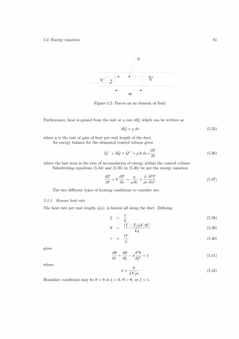
5.2. Energy equation 61
ds
Q Q_ +
Q
s
Figure 5.2: Forces on an element of fluid.
Furthermore, heat is gained from the side at a rate dQ, which can be written as
dQ = q ds (5.35)
where q is the rate of gain of heat per unit length of the duct.An energy balance for the elemental control volume gives
Q− + dQ = Q+ + ρA ds c∂T
∂t(5.36)
where the last term is the rate of accumulation of energy within the control volume.Substituting equations (5.34) and (5.35) in (5.36) we get the energy equation
∂T
∂t+ V
∂T
∂s=
q
ρAc+
k
ρc
∂2T
∂s2(5.37)
The two different types of heating conditions to consider are:
5.2.1 Known heat rate
The heat rate per unit length, q(s), is known all along the duct. Defining
ξ =x
L(5.38)
θ =(T − Ti)ρV AC
Lq(5.39)
τ =tV
L(5.40)
gives∂θ
∂τ+∂θ
∂ξ− λ
d2θ
dξ2= 1 (5.41)
where
λ =k
LV ρc(5.42)
Boundary conditions may be θ = 0 at ξ = 0, θ = θ1 at ξ = 1.
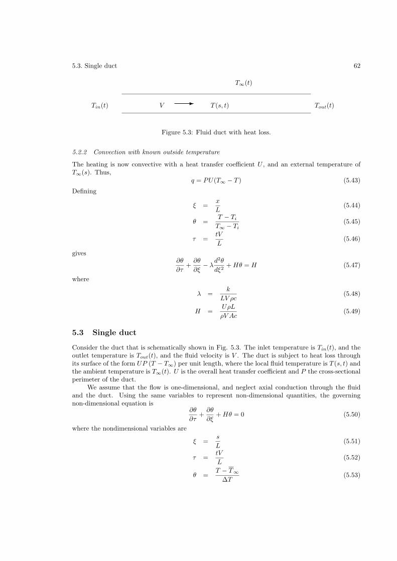
5.3. Single duct 62
Tin(t) T (s, t) Tout(t)
T∞(t)
V-
Figure 5.3: Fluid duct with heat loss.
5.2.2 Convection with known outside temperature
The heating is now convective with a heat transfer coefficient U , and an external temperature ofT∞(s). Thus,
q = PU(T∞ − T ) (5.43)
Defining
ξ =x
L(5.44)
θ =T − Ti
T∞ − Ti(5.45)
τ =tV
L(5.46)
gives∂θ
∂τ+∂θ
∂ξ− λ
d2θ
dξ2+Hθ = H (5.47)
where
λ =k
LV ρc(5.48)
H =UρL
ρV Ac(5.49)
5.3 Single duct
Consider the duct that is schematically shown in Fig. 5.3. The inlet temperature is Tin(t), and theoutlet temperature is Tout(t), and the fluid velocity is V . The duct is subject to heat loss throughits surface of the form UP (T − T∞) per unit length, where the local fluid temperature is T (s, t) andthe ambient temperature is T∞(t). U is the overall heat transfer coefficient and P the cross-sectionalperimeter of the duct.
We assume that the flow is one-dimensional, and neglect axial conduction through the fluidand the duct. Using the same variables to represent non-dimensional quantities, the governingnon-dimensional equation is
∂θ
∂τ+∂θ
∂ξ+Hθ = 0 (5.50)
where the nondimensional variables are
ξ =s
L(5.51)
τ =tV
L(5.52)
θ =T − T∞
∆T(5.53)
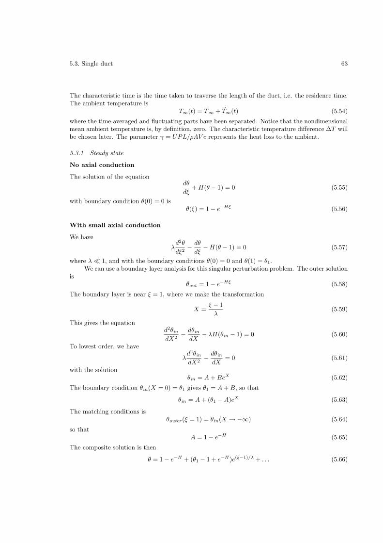
5.3. Single duct 63
The characteristic time is the time taken to traverse the length of the duct, i.e. the residence time.The ambient temperature is
T∞(t) = T∞ + T∞(t) (5.54)
where the time-averaged and fluctuating parts have been separated. Notice that the nondimensionalmean ambient temperature is, by definition, zero. The characteristic temperature difference ∆T willbe chosen later. The parameter γ = UPL/ρAV c represents the heat loss to the ambient.
5.3.1 Steady state
No axial conduction
The solution of the equationdθ
dξ+H(θ − 1) = 0 (5.55)
with boundary condition θ(0) = 0 isθ(ξ) = 1 − e−Hξ (5.56)
With small axial conduction
We have
λd2θ
dξ2− dθ
dξ−H(θ − 1) = 0 (5.57)
where λ≪ 1, and with the boundary conditions θ(0) = 0 and θ(1) = θ1.We can use a boundary layer analysis for this singular perturbation problem. The outer solution
isθout = 1 − e−Hξ (5.58)
The boundary layer is near ξ = 1, where we make the transformation
X =ξ − 1
λ(5.59)
This gives the equationd2θindX2
− dθindX
− λH(θin − 1) = 0 (5.60)
To lowest order, we have
λd2θindX2
− dθindX
= 0 (5.61)
with the solutionθin = A+BeX (5.62)
The boundary condition θin(X = 0) = θ1 gives θ1 = A+B, so that
θin = A+ (θ1 −A)eX (5.63)
The matching conditions isθouter (ξ = 1) = θin(X → −∞) (5.64)
so thatA = 1 − e−H (5.65)
The composite solution is then
θ = 1 − e−H + (θ1 − 1 + e−H)e(ξ−1)/λ + . . . (5.66)
5.3. Single duct 64
t
s
t = s
t < s
t > s
T (s, 0) = T0(s)
@@R
T (0, t) = Tin(t)
Figure 5.4: Solution in s-t space.
5.3.2 Unsteady dynamics
The general solution of this equation is
T (s, t) =
[f(s− t) + γ
∫ t
0
eHt′ T∞(t′) dt′]e−Ht (5.67)
The boundary conditions T (0, t) = Tin(t) and T (s, 0) = T0(s) are shown in Fig. 5.4. The solutionbecomes
T (s, t) =
Tin(t− s)e−Hs +He−Ht
∫ t
t−seHt′ T∞(t′) dt′ for t ≥ s
T0(s− t)e−Ht +He−Ht∫ t
0eHt′ T∞(t′) dt′ for t < s
(5.68)
The t < s part of the solution is applicable to the brief, transient period of time in which the fluidat time t = 0 has still not left the duct. The later t > s part depends on the temperature of thefluid entering at s = 0. The temperature, Tout(t), at the outlet section, s = 1, is given by
Tout(t) =
Tin(t− 1)e−H +He−Ht
∫ t
t−1eHt′ T∞(t′) dt′ for t ≥ 1
T0(1 − t)e−Ht +He−Ht∫ t
0eHt′ T∞(t′) dt′ for t < 1
(5.69)
It can be observed that, after an initial transient, the inlet and outlet temperatures are relatedby a unit delay. The outlet temperature is also affected by the heat loss parameter, γ, and theambient temperature fluctuation, T∞. The following are some special cases of equation (5.69).
5.3.3 Perfectly insulated duct
If H = 0 the outlet temperature simplifies to
Tout(t) =
Tin(t− 1) for t ≥ 1T0(1 − t) for t < 1
(5.70)
The outlet temperature is the same as the inlet temperature, but at a previous instant in time.
5.3.4 Constant ambient temperature
For this T∞ = 0, and equation (5.69) becomes
Tout(t) =
Tin(t− 1)e−H for t ≥ 1T0(1 − t)e−Ht for t < 1
(5.71)
This is similar to the above, but with an exponential drop due to heat transfer.
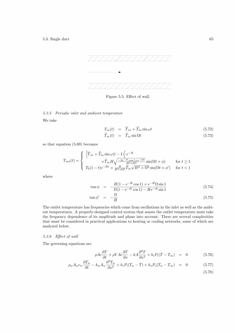
5.3. Single duct 65
Figure 5.5: Effect of wall.
5.3.5 Periodic inlet and ambient temperature
We take
Tin(t) = T in + Tin sinωt (5.72)
T∞(t) = T∞ sin Ωt (5.73)
so that equation (5.69) becomes
Tout(t) =
[T in + Tin sinω(t− 1)
]e−H
+T∞H√
−2e−H cos 1+e−2H
H2+Ω2 sin(Ωt+ φ) for t ≥ 1
T0(1 − t)e−Ht + HH2+Ω2 T∞
√H2 + Ω2 sin(Ωt+ φ′) for t < 1
where
tanφ = −H(1 − e−H cos 1) + e−HΩsin 1
Ω(1 − e−H cos 1) −He−H sin 1(5.74)
tanφ′ = − Ω
H(5.75)
The outlet temperature has frequencies which come from oscillations in the inlet as well as the ambi-ent temperatures. A properly-designed control system that senses the outlet temperature must takethe frequency dependence of its amplitude and phase into account. There are several complexitiesthat must be considered in practical applications to heating or cooling networks, some of which areanalyzed below.
5.3.6 Effect of wall
The governing equations are
ρAc∂T
∂t+ ρV Ac
∂T
∂x− kA
∂2T
∂x2+ hiPi(T − T∞) = 0 (5.76)
ρwAwcw∂Tw
∂t− kwAw
∂2Tw
∂x2+ hiPi(Tw − T ) + hoPo(Tw − T∞) = 0 (5.77)
(5.78)
5.4. Two-fluid configuration 66
Nondimensionalize, using
ξ =x
L(5.79)
τ =tV
L(5.80)
θ =T − T∞Ti − T∞
(5.81)
θw =Tw − T∞Ti − T∞
(5.82)
we get
∂θ
∂τ+∂θ
∂ξ− λ
∂2θ
∂ξ2+Hin(θ − θw) = 0 (5.83)
∂θw
∂τ− λw
∂2θw
∂ξ2+Hin(θw − θ) +Houtθw = 0 (5.84)
where
λw =kw
ρwV AwcwL(5.85)
Hin =hinPinL
ρwAwcwV(5.86)
Hout =houtPoutL
ρwAwcwV(5.87)
In the steady state and with no axial conduction in the fluid
dθ
dξ+Hin(θ − θw) = 0 (5.88)
−λwd2θw
dξ2+Hin(θw − θ) +Houtθw = 0 (5.89)
If we assume λw = 0 also, we get
θw =Hin
Hin +Houtθ (5.90)
The governing equation isdT
dξ+Hwθ = 0 (5.91)
where
Hw =Hw
inHwout
Hwin +Hw
out
(5.92)
5.4 Two-fluid configuration
Consider the heat balance in Fig. 5.6. Neglecting axial conduction, we have
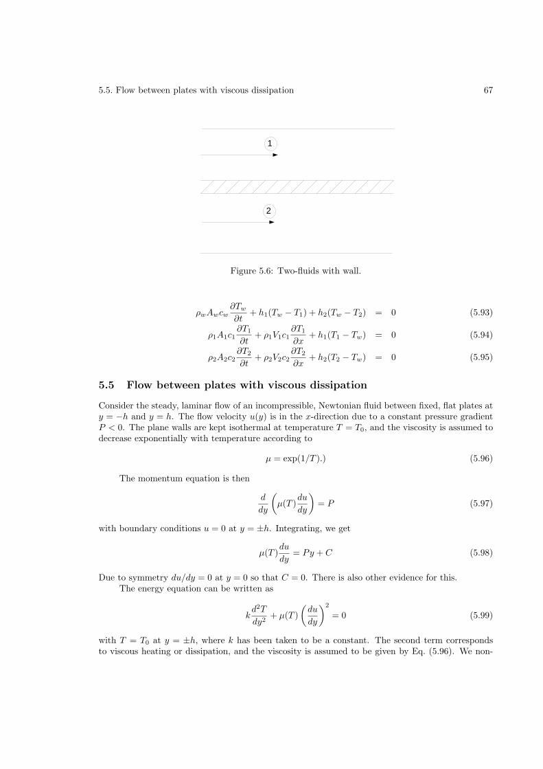
5.5. Flow between plates with viscous dissipation 67
1
2
Figure 5.6: Two-fluids with wall.
ρwAwcw∂Tw
∂t+ h1(Tw − T1) + h2(Tw − T2) = 0 (5.93)
ρ1A1c1∂T1
∂t+ ρ1V1c1
∂T1
∂x+ h1(T1 − Tw) = 0 (5.94)
ρ2A2c2∂T2
∂t+ ρ2V2c2
∂T2
∂x+ h2(T2 − Tw) = 0 (5.95)
5.5 Flow between plates with viscous dissipation
Consider the steady, laminar flow of an incompressible, Newtonian fluid between fixed, flat plates aty = −h and y = h. The flow velocity u(y) is in the x-direction due to a constant pressure gradientP < 0. The plane walls are kept isothermal at temperature T = T0, and the viscosity is assumed todecrease exponentially with temperature according to
µ = exp(1/T ).) (5.96)
The momentum equation is then
d
dy
(µ(T )
du
dy
)= P (5.97)
with boundary conditions u = 0 at y = ±h. Integrating, we get
µ(T )du
dy= Py + C (5.98)
Due to symmetry du/dy = 0 at y = 0 so that C = 0. There is also other evidence for this.The energy equation can be written as
kd2T
dy2+ µ(T )
(du
dy
)2
= 0 (5.99)
with T = T0 at y = ±h, where k has been taken to be a constant. The second term correspondsto viscous heating or dissipation, and the viscosity is assumed to be given by Eq. (5.96). We non-
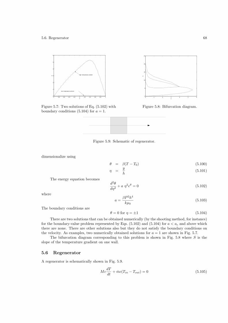
5.6. Regenerator 68
−1 −0.8 −0.6 −0.4 −0.2 0 0.2 0.4 0.6 0.8 10
1
2
3
4
5
6
η
θ
low−temperature solution
high−temperature solution
Figure 5.7: Two solutions of Eq. (5.102) withboundary conditions (5.104) for a = 1.
0 1 2 3 4 5 60
5
10
15
20
25
a
S
Figure 5.8: Bifurcation diagram.
Figure 5.9: Schematic of regenerator.
dimensionalize using
θ = β(T − T0) (5.100)
η =y
h(5.101)
The energy equation becomesd2θ
dη2+ a η2eθ = 0 (5.102)
where
a =βP 2h4
kµ0(5.103)
The boundary conditions areθ = 0 for η = ±1 (5.104)
There are two solutions that can be obtained numerically (by the shooting method, for instance)for the boundary-value problem represented by Eqs. (5.102) and (5.104) for a < ac and above whichthere are none. There are other solutions also but they do not satisfy the boundary conditions onthe velocity. As examples, two numerically obtained solutions for a = 1 are shown in Fig. 5.7.
The bifurcation diagram corresponding to this problem is shown in Fig. 5.8 where S is theslope of the temperature gradient on one wall.
5.6 Regenerator
A regenerator is schematically shown in Fig. 5.9.
McdT
dt+ mc(Tin − Tout) = 0 (5.105)
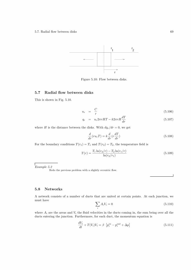
5.7. Radial flow between disks 69
r
r r1 2
Figure 5.10: Flow between disks.
5.7 Radial flow between disks
This is shown in Fig. 5.10.
ur =C
r(5.106)
qr = ur2πrHT − k2πrHdT
dr(5.107)
where H is the distance between the disks. With dqr/dr = 0, we get
d
dr(rurT ) = k
d
dr(rdT
dr) (5.108)
For the boundary conditions T (r1) = T1 and T (r2) = T2, the temperature field is
T (r) =T1 ln(r2/r) − T2 ln(r1/r)
ln(r2/r1)(5.109)
Example 5.2Redo the previous problem with a slightly eccentric flow.
5.8 Networks
A network consists of a number of ducts that are united at certain points. At each junction, wemust have ∑
i
AiVi = 0 (5.110)
where Ai are the areas and Vi the fluid velocities in the ducts coming in, the sum being over all theducts entering the junction. Furthermore, for each duct, the momentum equation is
dVi
dt+ T (Vi)Vi = β
[pin
i − pouti + ∆p
](5.111)
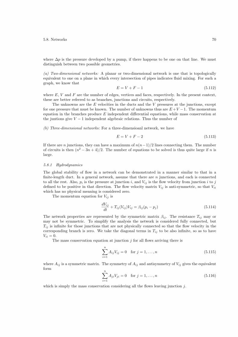
5.8. Networks 70
where ∆p is the pressure developed by a pump, if there happens to be one on that line. We mustdistinguish between two possible geometries.
(a) Two-dimensional networks: A planar or two-dimensional network is one that is topologicallyequivalent to one on a plane in which every intersection of pipes indicates fluid mixing. For such agraph, we know that
E = V + F − 1 (5.112)
where E, V and F are the number of edges, vertices and faces, respectively. In the present context,these are better referred to as branches, junctions and circuits, respectively.
The unknowns are the E velocities in the ducts and the V pressures at the junctions, exceptfor one pressure that must be known. The number of unknowns thus are E+V −1. The momentumequation in the branches produce E independent differential equations, while mass conservation atthe juntions give V − 1 independent algebraic relations. Thus the number of
(b) Three-dimensional networks: For a three-dimensioanl network, we have
E = V + F − 2 (5.113)
If there are n junctions, they can have a maximum of n(n−1)/2 lines connecting them. The numberof circuits is then (n2 − 3n+ 4)/2. The number of equations to be solved is thus quite large if n islarge.
5.8.1 Hydrodynamics
The global stability of flow in a network can be demonstrated in a manner similar to that in afinite-length duct. In a general network, assume that there are n junctions, and each is connectedto all the rest. Also, pi is the pressure at junction i, and Vij is the flow velocity from junction i to jdefined to be positive in that direction. The flow velocity matrix Vij is anti-symmetric, so that Vii
which has no physical meaning is considered zero.The momentum equation for Vij is
dVij
dt+ Tij(Vij)Vij = βij(pi − pj) (5.114)
The network properties are represented by the symmetric matrix βij . The resistance Tij may ormay not be symmetric. To simplify the analysis the network is considered fully connected, butTij is infinite for those junctions that are not physically connected so that the flow velocity in thecorresponding branch is zero. We take the diagonal terms in Tij to be also infinite, so as to haveVii = 0.
The mass conservation equation at junction j for all flows arriving there is
n∑
i=1
AijVij = 0 for j = 1, . . . , n (5.115)
where Aij is a symmetric matrix. The symmetry of Aij and antisymmetry of Vij gives the equivalentform
n∑
i=1
AjiVji = 0 for j = 1, . . . , n (5.116)
which is simply the mass conservation considering all the flows leaving junction j.
5.8. Networks 71
The steady states are solutions of
Tij(V ij)V ij = βij(pi − pj) (5.117)n∑
i=1
AijV ij = 0 orn∑
i=1
AjiV ji = 0 (5.118)
We write
Vij = V ij + V ′
ij (5.119)
pi = p+ p′i (5.120)
Substituting in equations (5.114)–(5.116), and subtracting equations (5.117) and (5.118) we get
dV ′
ij
dt= −
[Tij(V ij + V ′
ij)(V ij + V ′
ij) − Tij(V ij)V ij
]+ βij(p
′
i − p′j) (5.121)
n∑
i=1
AijV′
ij = 0 orn∑
i=1
AjiV′
ji = 0 (5.122)
Defining
E =1
2
n∑
j=1
n∑
i=1
Aij
βijV ′2
ij , βij > 0 (5.123)
we get
dE
dt=
n∑
j=1
n∑
i=1
Aij
βijV ′
ij
dV ′
ij
dt(5.124)
= −n∑
j=1
n∑
i=1
Aij
βijV ′
ij
[Tij(V ij + V ′
ij)(V ij + V ′
ij) − Tij(V ij)V ij
]
+
n∑
j=1
n∑
i=1
AijV′
ij(p′
i − p′j) (5.125)
The pressure terms vanish since
n∑
j=1
n∑
i=1
AijV′
ijp′
i =n∑
i=1
n∑
j=1
AijV′
ijp′
i (5.126)
=
n∑
i=1
p′i
n∑
j=1
AijV′
ij
(5.127)
= 0 (5.128)
and
n∑
j=1
n∑
i=1
AijV′
ijp′
j =n∑
j=1
(p′j
n∑
i=1
AijV′
ij
)(5.129)
= 0 (5.130)
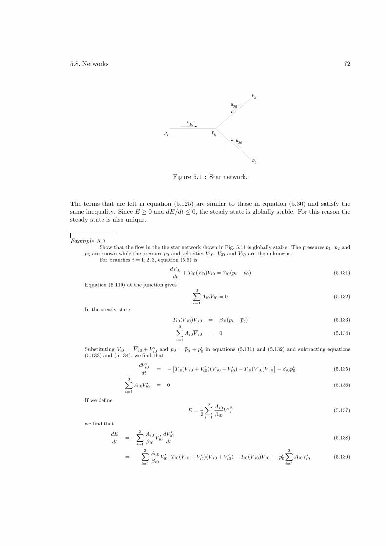
5.8. Networks 72
p1
p2
p3
u10
u30
u20
p0
Figure 5.11: Star network.
The terms that are left in equation (5.125) are similar to those in equation (5.30) and satisfy thesame inequality. Since E ≥ 0 and dE/dt ≤ 0, the steady state is globally stable. For this reason thesteady state is also unique.
Example 5.3Show that the flow in the the star network shown in Fig. 5.11 is globally stable. The pressures p1, p2 and
p3 are known while the pressure p0 and velocities V10, V20 and V30 are the unknowns.For branches i = 1, 2, 3, equation (5.6) is
dVi0
dt+ Ti0(Vi0)Vi0 = βi0(pi − p0) (5.131)
Equation (5.110) at the junction gives3X
i=1
Ai0Vi0 = 0 (5.132)
In the steady state
Ti0(V i0)V i0 = βi0(pi − p0) (5.133)
3X
i=1
Ai0V i0 = 0 (5.134)
Substituting Vi0 = V i0 + V ′
i0 and p0 = p0 + p′0 in equations (5.131) and (5.132) and subtracting equations(5.133) and (5.134), we find that
dV ′
i0
dt= −
ˆ
Ti0(V i0 + V ′
i0)(V i0 + V ′
i0) − Ti0(V i0)V i0
˜
− βi0p′0 (5.135)
3X
i=1
Ai0V ′
i0 = 0 (5.136)
If we define
E =1
2
3X
i=1
Ai0
βi0V ′2
i (5.137)
we find that
dE
dt=
3X
i=1
Ai0
βi0V ′
i0
dV ′
i0
dt(5.138)
= −3X
i=1
Ai0
βi0V ′
i0
ˆ
Ti0(V i0 + V ′
i0)(V i0 + V ′
i0) − Ti0(V i0)V i0
˜
− p′0
3X
i=1
Ai0V ′
i0 (5.139)
5.9. Thermal control 73
The last term vanishes because of equation (5.136). Thus
dE
dt= −
3X
i=1
Ai0
βi0V ′
i0V i0
ˆ
Ti0(V i0 + V ′
i0) − Ti0(V i0)˜
−3X
i=1
Ai0
βi0V ′2
i0Ti0(V i0 + V ′
i0) (5.140)
Since E ≥ 0 and dE/dt ≤ 0, E is a Lyapunov function and the steady state is globally stable.
5.8.2 Thermal networks
[61]
5.9 Thermal control
5.9.1 Control with heat transfer coefficient
5.9.2 Multiple room temperatures
Let there be n interconnected rooms. The wall temperature of room i is Twi and the air temperature
is T ai . The heat balance equation for this room is
Mai c
w dTwi
dt= hiAi(T
ai − Tw
i ) + UiAei (T
e − Twi ) (5.141)
Mai c
a dTai
dt= hiAi(T
wi − T a
i ) +1
2ca∑
j
(maji + |ma
ji|)T aj
−1
2ca∑
j
(maij + |ma
ij |)T ai + qi (5.142)
where T e is the exterior temperature, mij is the mass flow rate of air from room i to room j. Bydefinition mij = −mji. Since mii has no meaning and can be arbitrarily taken to be zero, mij is ananti-symmetric matrix. Also, from mass conservation for a single room, we know that
∑
j
maji = 0 (5.143)
Analysis
The unknowns in equations (5.141) and (5.142) are the 2n temperatures Twi and T a
i .(i) Steady state with U = 0(a) The equality ∑
i
∑
j
(maji + |ma
ji|)T aj −
∑
i
∑
j
(maij + |ma
ij |)T ai = 0 (5.144)
can be shown by interchanging i and j in the second term. Using this result, the sum of equations(5.141) and (5.142) for all rooms gives ∑
i
qi = 0 (5.145)
which is a necessary condition for a steady state.(b) Because the sum of equations (5.141) and (5.142) for all rooms gives an identity, the set ofequations is not linearly independent. Thus the steady solution is not unique unless one of the roomtemperatures is known.
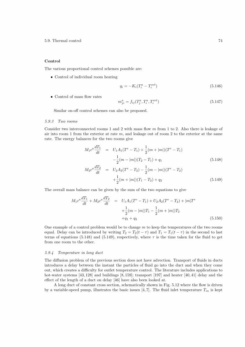
5.9. Thermal control 74
Control
The various proportional control schemes possible are:
• Control of individual room heating
qi = −Ki(Tai − T set
i ) (5.146)
• Control of mass flow ratesma
ji = fij(Taj , T
ai , T
seti ) (5.147)
Similar on-off control schemes can also be proposed.
5.9.3 Two rooms
Consider two interconnected rooms 1 and 2 with mass flow m from 1 to 2. Also there is leakage ofair into room 1 from the exterior at rate m, and leakage out of room 2 to the exterior at the samerate. The energy balances for the two rooms give
M1ca dT1
dt= U1A1(T
e − T1) +1
2(m+ |m|)(T e − T1)
−1
2(m− |m|)(T2 − T1) + q1 (5.148)
M2ca dT2
dt= U2A2(T
e − T2) −1
2(m− |m|)(T e − T2)
+1
2(m+ |m|)(T1 − T2) + q2 (5.149)
The overall mass balance can be given by the sum of the two equations to give
M1ca dT1
dt+M2c
a dT2
dt= U1A1(T
e − T1) + U2A2(Te − T2) + |m|T e
+1
2(m− |m|)T1 −
1
2(m+ |m|)T2
+q1 + q2 (5.150)
One example of a control problem would be to change m to keep the temperatures of the two roomsequal. Delay can be introduced by writing T2 = T2(t− τ) and T1 = T1(t− τ) in the second to lastterms of equations (5.148) and (5.149), respectively, where τ is the time taken for the fluid to getfrom one room to the other.
5.9.4 Temperature in long duct
The diffusion problem of the previous section does not have advection. Transport of fluids in ductsintroduces a delay between the instant the particles of fluid go into the duct and when they comeout, which creates a difficulty for outlet temperature control. The literature includes applications tohot-water systems [43, 128] and buildings [8, 159]; transport [197] and heater [40, 41] delay and theeffect of the length of a duct on delay [46] have also been looked at.
A long duct of constant cross section, schematically shown in Fig. 5.12 where the flow is drivenby a variable-speed pump, illustrates the basic issues [4, 7]. The fluid inlet temperature Tin is kept
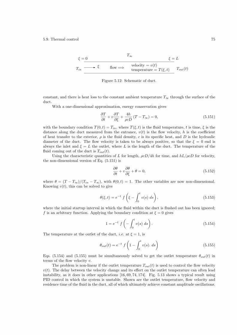
5.9. Thermal control 75
- =⇒flowvelocity = v(t)temperature = T (ξ, t)
ξ
ξ = 0 ξ = L
Tin Tout(t)
T∞
Figure 5.12: Schematic of duct.
constant, and there is heat loss to the constant ambient temperature T∞ through the surface of theduct.
With a one-dimensional approximation, energy conservation gives
∂T
∂t+ v
∂T
∂ξ+
4h
ρcD(T − T∞) = 0, (5.151)
with the boundary condition T (0, t) = Tin, where T (ξ, t) is the fluid temperature, t is time, ξ is thedistance along the duct measured from the entrance, v(t) is the flow velocity, h is the coefficientof heat transfer to the exterior, ρ is the fluid density, c is its specific heat, and D is the hydraulicdiameter of the duct. The flow velocity is taken to be always positive, so that the ξ = 0 end isalways the inlet and ξ = L the outlet, where L is the length of the duct. The temperature of thefluid coming out of the duct is Tout(t).
Using the characteristic quantities of L for length, ρcD/4h for time, and hL/ρcD for velocity,the non-dimensional version of Eq. (5.151) is
∂θ
∂t+ v
∂θ
∂ξ+ θ = 0, (5.152)
where θ = (T − T∞)/(Tin − T∞), with θ(0, t) = 1. The other variables are now non-dimensional.Knowing v(t), this can be solved to give
θ(ξ, t) = e−t f
(ξ −
∫ t
0
v(s) ds
), (5.153)
where the initial startup interval in which the fluid within the duct is flushed out has been ignored;f is an arbitrary function. Applying the boundary condition at ξ = 0 gives
1 = e−t f
(−∫ t
0
v(s) ds
). (5.154)
The temperature at the outlet of the duct, i.e. at ξ = 1, is
θout(t) = e−t f
(1 −
∫ t
0
v(s). ds
)(5.155)
Eqs. (5.154) and (5.155) must be simultaneously solved to get the outlet temperature θout(t) interms of the flow velocity v.
The problem is non-linear if the outlet temperature Tout(t) is used to control the flow velocityv(t). The delay between the velocity change and its effect on the outlet temperature can often leadinstability, as it does in other applications [16, 69, 74, 174]. Fig. 5.13 shows a typical result usingPID control in which the system is unstable. Shown are the outlet temperature, flow velocity andresidence time of the fluid in the duct, all of which ultimately achieve constant amplitude oscillations.
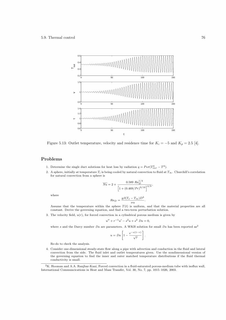
5.9. Thermal control 76
0 50 100 1500.2
0.3
0.4
0.5
Tou
t
0 50 100 1500.5
1
1.5
v
0 50 100 1500.6
0.8
1
1.2
1.4
t
τ
Figure 5.13: Outlet temperature, velocity and residence time for Ki = −5 and Kp = 2.5 [4].
Problems
1. Determine the single duct solutions for heat loss by radiation q = Pǫσ(T 4sur − T 4).
2. A sphere, initially at temperature Ti is being cooled by natural convection to fluid at T∞. Churchill’s correlationfor natural convection from a sphere is
Nu = 2 +0.589 Ra
1/4D
h
1 + (0.469/Pr)9/16i4/9
,
where
RaD =gβ(Ts − T∞)D3
να.
Assume that the temperature within the sphere T (t) is uniform, and that the material properties are allconstant. Derive the governing equation, and find a two-term perturbation solution.
3. The velocity field, u(r), for forced convection in a cylindrical porous medium is given by
u′′ + r−1u′ − s2u + s2 Da = 0,
where s and the Darcy number Da are parameters. A WKB solution for small Da has been reported as2
u = Da
"
1 − e−s(1−r)
√r
#
.
Re-do to check the analysis.
4. Consider one-dimensional steady-state flow along a pipe with advection and conduction in the fluid and lateralconvection from the side. The fluid inlet and outlet temperatures given. Use the nondimensional version ofthe governing equation to find the inner and outer matched temperature distributions if the fluid thermalconductivity is small.
2K. Hooman and A.A. Ranjbar-Kani, Forced convection in a fluid-saturated porous-medium tube with isoflux wall,International Communcications in Heat and Mass Transfer, Vol. 30, No. 7, pp. 1015–1026, 2003.
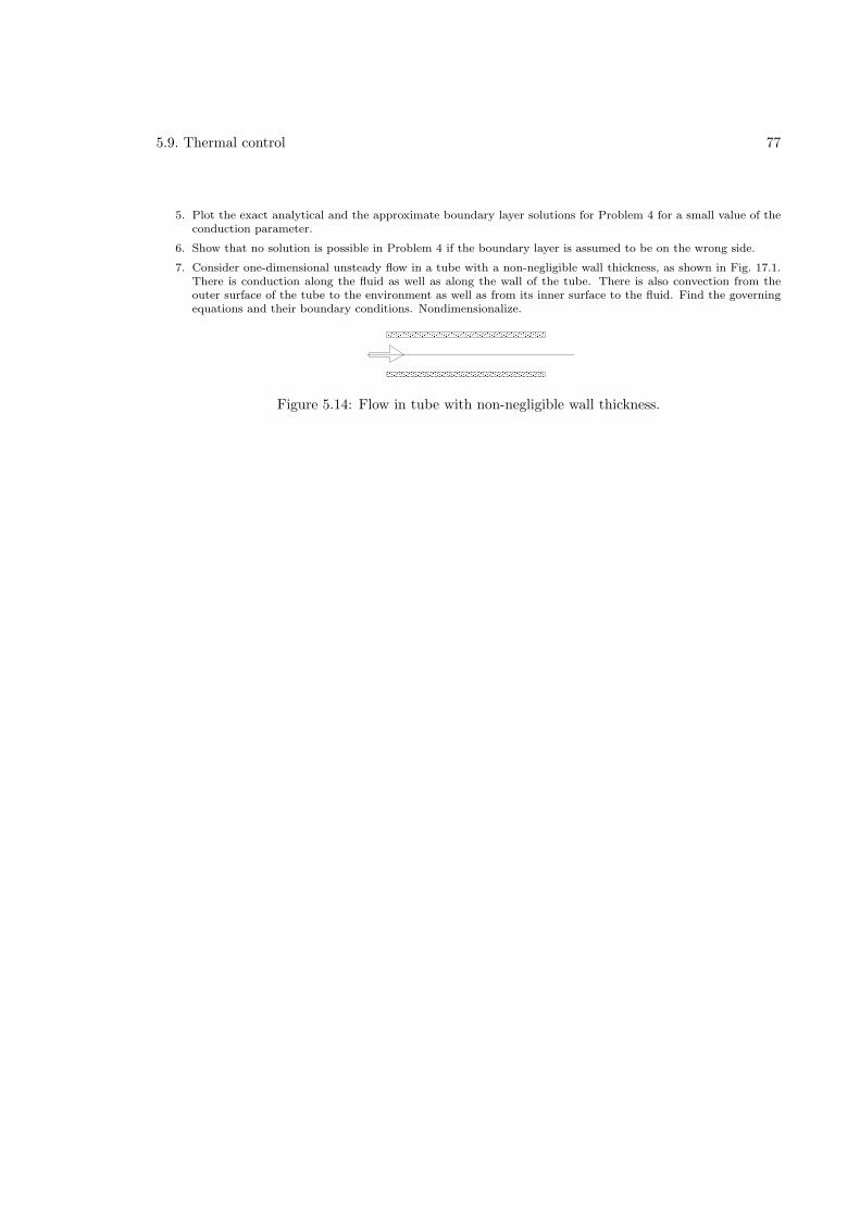
5.9. Thermal control 77
5. Plot the exact analytical and the approximate boundary layer solutions for Problem 4 for a small value of theconduction parameter.
6. Show that no solution is possible in Problem 4 if the boundary layer is assumed to be on the wrong side.
7. Consider one-dimensional unsteady flow in a tube with a non-negligible wall thickness, as shown in Fig. 17.1.There is conduction along the fluid as well as along the wall of the tube. There is also convection from theouter surface of the tube to the environment as well as from its inner surface to the fluid. Find the governingequations and their boundary conditions. Nondimensionalize.
Figure 5.14: Flow in tube with non-negligible wall thickness.
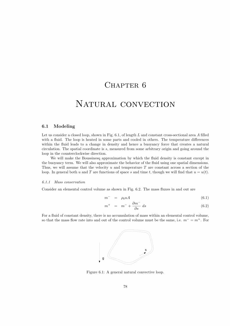
Chapter 6
Natural convection
6.1 Modeling
Let us consider a closed loop, shown in Fig. 6.1, of length L and constant cross-sectional area A filledwith a fluid. The loop is heated in some parts and cooled in others. The temperature differenceswithin the fluid leads to a change in density and hence a buoyancy force that creates a naturalcirculation. The spatial coordinate is s, measured from some arbitrary origin and going around theloop in the counterclockwise direction.
We will make the Boussinesq approximation by which the fluid density is constant except inthe buoyancy term. We will also approximate the behavior of the fluid using one spatial dimensions.Thus, we will assume that the velocity u and temperature T are constant across a section of theloop. In general both u and T are functions of space s and time t, though we will find that u = u(t).
6.1.1 Mass conservation
Consider an elemental control volume as shown in Fig. 6.2. The mass fluxes in and out are
m− = ρ0uA (6.1)
m+ = m− +∂m−
∂sds (6.2)
For a fluid of constant density, there is no accumulation of mass within an elemental control volume,so that the mass flow rate into and out of the control volume must be the same, i.e. m− = m+. For
s
g
Figure 6.1: A general natural convective loop.
78
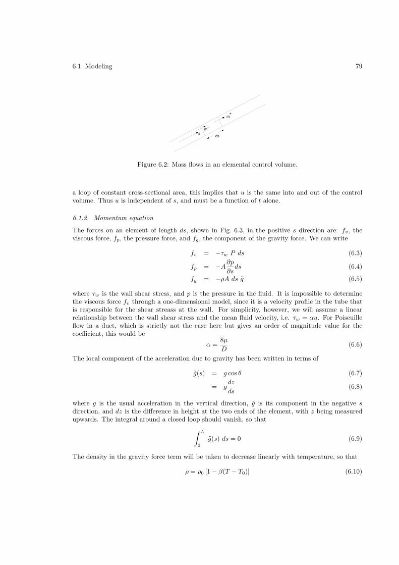
6.1. Modeling 79
sds
m+
m_
Figure 6.2: Mass flows in an elemental control volume.
a loop of constant cross-sectional area, this implies that u is the same into and out of the controlvolume. Thus u is independent of s, and must be a function of t alone.
6.1.2 Momentum equation
The forces on an element of length ds, shown in Fig. 6.3, in the positive s direction are: fv, theviscous force, fp, the pressure force, and fg, the component of the gravity force. We can write
fv = −τw P ds (6.3)
fp = −A∂p∂sds (6.4)
fg = −ρA ds g (6.5)
where τw is the wall shear stress, and p is the pressure in the fluid. It is impossible to determinethe viscous force fv through a one-dimensional model, since it is a velocity profile in the tube thatis responsible for the shear streass at the wall. For simplicity, however, we will assume a linearrelationship between the wall shear stress and the mean fluid velocity, i.e. τw = αu. For Poiseuilleflow in a duct, which is strictly not the case here but gives an order of magnitude value for thecoefficient, this would be
α =8µ
D(6.6)
The local component of the acceleration due to gravity has been written in terms of
g(s) = g cos θ (6.7)
= gdz
ds(6.8)
where g is the usual acceleration in the vertical direction, g is its component in the negative sdirection, and dz is the difference in height at the two ends of the element, with z being measuredupwards. The integral around a closed loop should vanish, so that
∫ L
0
g(s) ds = 0 (6.9)
The density in the gravity force term will be taken to decrease linearly with temperature, so that
ρ = ρ0 [1 − β(T − T0)] (6.10)
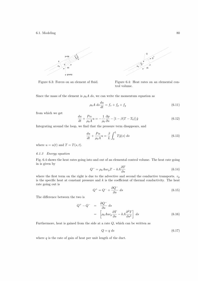
6.1. Modeling 80
p
p+dp
gravity
fff
v
pg
sds
θ
Figure 6.3: Forces on an element of fluid.
sds
Q
Q+
Q_
Figure 6.4: Heat rates on an elemental con-trol volume.
Since the mass of the element is ρ0A ds, we can write the momentum equation as
ρ0A dsdu
dt= fv + fp + fg (6.11)
from which we getdu
dt+Pα
ρ0Au = − 1
ρ0
∂p
∂s− [1 − β(T − T0)] g (6.12)
Integrating around the loop, we find that the pressure term disappears, and
du
dt+Pα
ρ0Au =
β
L
∫ L
0
T g(s) ds (6.13)
where u = u(t) and T = T (s, t).
6.1.3 Energy equation
Fig. 6.4 shows the heat rates going into and out of an elemental control volume. The heat rate goingin is given by
Q− = ρ0AucpT − kA∂T
∂s(6.14)
where the first term on the right is due to the advective and second the conductive transports. cpis the specific heat at constant pressure and k is the coefficient of thermal conductivity. The heatrate going out is
Q+ = Q− +∂Q−
∂sds (6.15)
The difference between the two is
Q+ −Q− =∂Q−
∂sds
=
[ρ0Aucp
∂T
∂s− kA
∂2T
∂s2
]ds (6.16)
Furthermore, heat is gained from the side at a rate Q, which can be written as
Q = q ds (6.17)
where q is the rate of gain of heat per unit length of the duct.
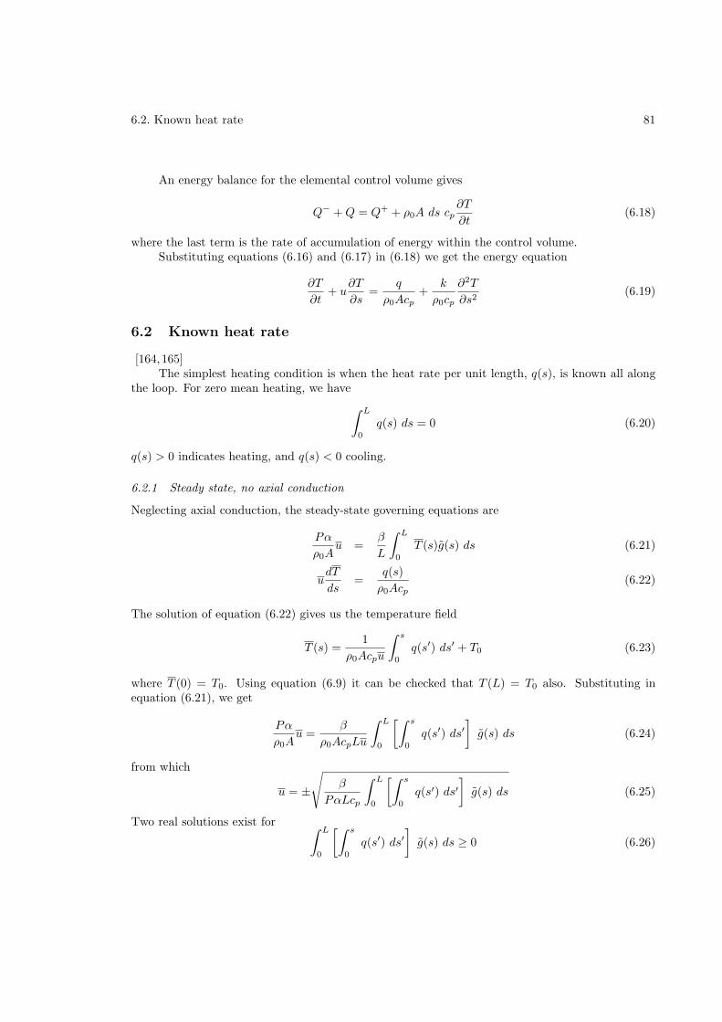
6.2. Known heat rate 81
An energy balance for the elemental control volume gives
Q− +Q = Q+ + ρ0A ds cp∂T
∂t(6.18)
where the last term is the rate of accumulation of energy within the control volume.Substituting equations (6.16) and (6.17) in (6.18) we get the energy equation
∂T
∂t+ u
∂T
∂s=
q
ρ0Acp+
k
ρ0cp
∂2T
∂s2(6.19)
6.2 Known heat rate
[164,165]The simplest heating condition is when the heat rate per unit length, q(s), is known all along
the loop. For zero mean heating, we have
∫ L
0
q(s) ds = 0 (6.20)
q(s) > 0 indicates heating, and q(s) < 0 cooling.
6.2.1 Steady state, no axial conduction
Neglecting axial conduction, the steady-state governing equations are
Pα
ρ0Au =
β
L
∫ L
0
T (s)g(s) ds (6.21)
udT
ds=
q(s)
ρ0Acp(6.22)
The solution of equation (6.22) gives us the temperature field
T (s) =1
ρ0Acpu
∫ s
0
q(s′) ds′ + T0 (6.23)
where T (0) = T0. Using equation (6.9) it can be checked that T (L) = T0 also. Substituting inequation (6.21), we get
Pα
ρ0Au =
β
ρ0AcpLu
∫ L
0
[∫ s
0
q(s′) ds′]g(s) ds (6.24)
from which
u = ±√
β
PαLcp
∫ L
0
[∫ s
0
q(s′) ds′]g(s) ds (6.25)
Two real solutions exist for ∫ L
0
[∫ s
0
q(s′) ds′]g(s) ds ≥ 0 (6.26)
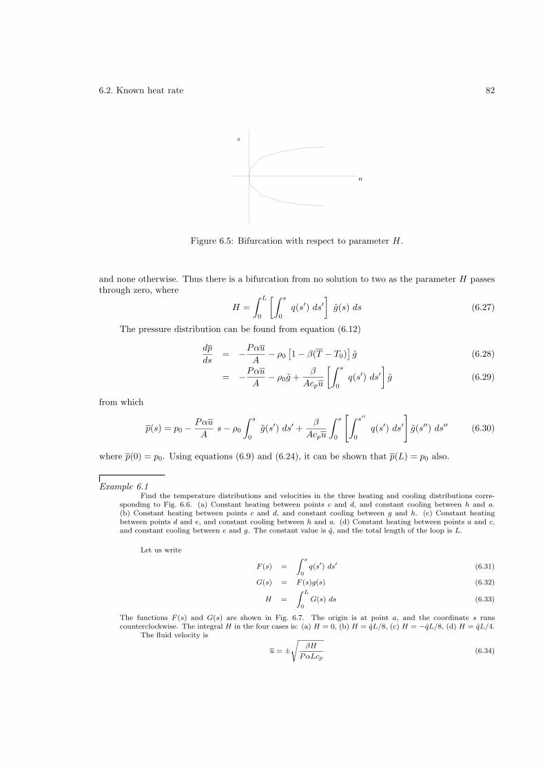
6.2. Known heat rate 82
u
H
Figure 6.5: Bifurcation with respect to parameter H.
and none otherwise. Thus there is a bifurcation from no solution to two as the parameter H passesthrough zero, where
H =
∫ L
0
[∫ s
0
q(s′) ds′]g(s) ds (6.27)
The pressure distribution can be found from equation (6.12)
dp
ds= −Pαu
A− ρ0
[1 − β(T − T0)
]g (6.28)
= −PαuA
− ρ0g +β
Acpu
[∫ s
0
q(s′) ds′]g (6.29)
from which
p(s) = p0 −Pαu
As− ρ0
∫ s
0
g(s′) ds′ +β
Acpu
∫ s
0
[∫ s′′
0
q(s′) ds′
]g(s′′) ds′′ (6.30)
where p(0) = p0. Using equations (6.9) and (6.24), it can be shown that p(L) = p0 also.
Example 6.1Find the temperature distributions and velocities in the three heating and cooling distributions corre-
sponding to Fig. 6.6. (a) Constant heating between points c and d, and constant cooling between h and a.(b) Constant heating between points c and d, and constant cooling between g and h. (c) Constant heatingbetween points d and e, and constant cooling between h and a. (d) Constant heating between points a and c,and constant cooling between e and g. The constant value is q, and the total length of the loop is L.
Let us write
F (s) =
Z s
0q(s′) ds′ (6.31)
G(s) = F (s)g(s) (6.32)
H =
Z L
0G(s) ds (6.33)
The functions F (s) and G(s) are shown in Fig. 6.7. The origin is at point a, and the coordinate s runscounterclockwise. The integral H in the four cases is: (a) H = 0, (b) H = qL/8, (c) H = −qL/8, (d) H = qL/4.
The fluid velocity is
u = ±s
βH
PαLcp(6.34)
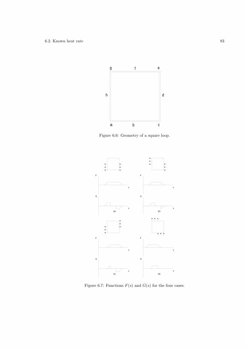
6.2. Known heat rate 83
a b c
d
efg
h
Figure 6.6: Geometry of a square loop.
F
G
s
s
F
G
s
s
F
G
s
s
(a) (b)
F
G
s
s
(c) (d)
Figure 6.7: Functions F (s) and G(s) for the four cases.
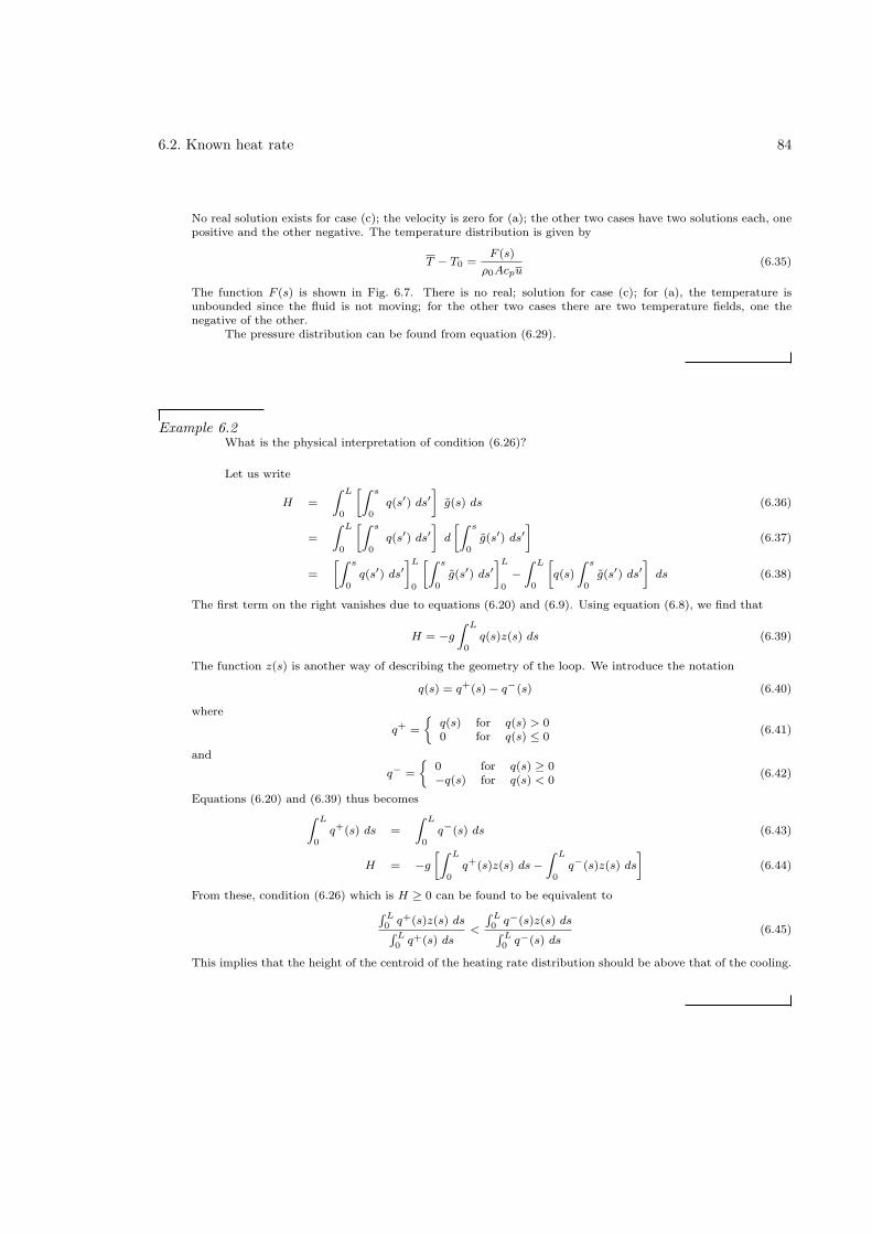
6.2. Known heat rate 84
No real solution exists for case (c); the velocity is zero for (a); the other two cases have two solutions each, onepositive and the other negative. The temperature distribution is given by
T − T0 =F (s)
ρ0Acpu(6.35)
The function F (s) is shown in Fig. 6.7. There is no real; solution for case (c); for (a), the temperature isunbounded since the fluid is not moving; for the other two cases there are two temperature fields, one thenegative of the other.
The pressure distribution can be found from equation (6.29).
Example 6.2What is the physical interpretation of condition (6.26)?
Let us write
H =
Z L
0
»Z s
0q(s′) ds′
–
g(s) ds (6.36)
=
Z L
0
»Z s
0q(s′) ds′
–
d
»Z s
0g(s′) ds′
–
(6.37)
=
»Z s
0q(s′) ds′
–L
0
»Z s
0g(s′) ds′
–L
0
−Z L
0
»
q(s)
Z s
0g(s′) ds′
–
ds (6.38)
The first term on the right vanishes due to equations (6.20) and (6.9). Using equation (6.8), we find that
H = −g
Z L
0q(s)z(s) ds (6.39)
The function z(s) is another way of describing the geometry of the loop. We introduce the notation
q(s) = q+(s) − q−(s) (6.40)
where
q+ =
q(s) for q(s) > 00 for q(s) ≤ 0
(6.41)
and
q− =
0 for q(s) ≥ 0−q(s) for q(s) < 0
(6.42)
Equations (6.20) and (6.39) thus becomes
Z L
0q+(s) ds =
Z L
0q−(s) ds (6.43)
H = −g
»Z L
0q+(s)z(s) ds −
Z L
0q−(s)z(s) ds
–
(6.44)
From these, condition (6.26) which is H ≥ 0 can be found to be equivalent to
R L0 q+(s)z(s) dsR L0 q+(s) ds
<
R L0 q−(s)z(s) dsR L0 q−(s) ds
(6.45)
This implies that the height of the centroid of the heating rate distribution should be above that of the cooling.
6.2. Known heat rate 85
6.2.2 Axial conduction effects
To nondimensionalize and normalize equations (6.13) and (6.19), we take
t∗ =t
τ(6.46)
s∗ =s
L(6.47)
u∗ =u
V G1/2(6.48)
T ∗ =T − T0
∆T G1/2(6.49)
g∗ =g
g(6.50)
q∗ =q
qm(6.51)
where
V =PαL
ρ0A(6.52)
∆T =P 2α2L
βgρ20A
2(6.53)
τ =ρ0A
Pα(6.54)
G =qmβgρ
20A
2
P 3α3Lcp(6.55)
Substituting, we get
du∗
dt∗+ u∗ =
∫ 1
0
T ∗g∗ ds∗ (6.56)
∂T ∗
∂t∗+G1/2u∗
∂T ∗
∂s∗= G1/2q∗ +K
∂2T ∗
∂s∗2(6.57)
where
K =kA
PαL2cp(6.58)
The two nondimensional parameters which govern the problem are G and K.Under steady-state conditions, and neglecting axial conduction, the temperature and velocity
are
T∗
(s) =1
u∗
∫ s∗
0
q∗(s∗1) ds∗
1 (6.59)
u∗ = ±√∫ 1
0
[∫ s∗
0
q∗(s∗1) ds∗
1
]g∗(s∗) ds∗ (6.60)
All variables are of unit order indicating that the variables have been appropriately normalized.
6.2. Known heat rate 86
For α = 8µ/D, A = πD2/4, and P = πD, we get
G =1
8192π
Gr
Pr
(D
L
)4
(6.61)
K =1
32 Pr
(D
L
)2
(6.62)
where the Prandtl and Grashof numbers are
Pr =µcpk
(6.63)
Gr =qmgβL
3
ν2k(6.64)
respectively. Often the Rayleigh number defined by
Ra = Gr Pr (6.65)
is used instead of the Grashof number.Since u∗ is of O(1), the dimensional velocity is of order (8νL/D2)Gr1/2. The ratio of axial
conduction to the advective transport term is
ǫ =K
G1/2(6.66)
=
(8π
Ra
)1/2
(6.67)
Taking typical numerical values for a loop with water to be: ρ = 998 kg/m3, µ = 1.003×10⁻³ kg/ms, k = 0.6 W/m K, qm = 100 W/m, g = 9.91 m/s2, β = 0.207 × 10⁻³ K−1, D = 0.01 m, L = 1 m,cp = 4.18 × 10³ J/kgK, we get the velocity and temperature scales to be
V G1/2 = (6.68)
∆TG1/2 = (6.69)
and the nondimensional numbers as
G = 1.86 × 10⁻² (6.70)
K = 4.47 × 10⁻⁷ (6.71)
Gr = 3.35 × 10¹¹ (6.72)
Ra = 2.34 × 10¹² (6.73)
ǫ = 3.28 × 10⁻⁶ (6.74)
Axial conduction is clearly negligible in this context.For a steady state, equations (6.56) and (6.57) are
u∗ =
∫ 1
0
T∗
g∗ ds∗ (6.75)
ǫd2T
∗
ds∗2− u∗
dT∗
ds∗= −q∗(s∗) (6.76)
Integrating over the loop from s∗ = 0 to s∗ = 1, we find that continuity of T∗
and equation (6.20)
imply continuity of dT∗
/ds∗ also.
6.2. Known heat rate 87
Conduction-dominated flow
If λ = G1/2/ǫ≪ 1, axial conduction dominates. We can write
u = u0 + λu1 + λ2u2 + . . . (6.77)
T (s) = T 0(s) + λT 1(s) + λ2T 2(s) + . . . (6.78)
where, for convenience, the asterisks have been dropped. Substituting into the governing equations,and collecting terms of O(λ0), we have
u0 =
∫ 1
0
T 0g ds (6.79)
d2T 0
ds2= 0 (6.80)
The second equation, along with conditions that T 0 and dT 0/ds have the same value at s = 0 ands = 1, gives T 0 = an arbitrary constant. The first equation gives u0 = 0.
The terms of O(λ) give
u1 =
∫ 1
0
T 1g ds (6.81)
d2T 1
ds2= −q(s) + u0
dT 0
ds(6.82)
The second equation can be integrated once to give
dT 1
ds= −
∫ s
0
q(s′) ds′ +A (6.83)
and again
T 1 = −∫ s
0
[∫ s′′
0
q(s′) ds′
]ds′′ +As+B (6.84)
Continuity of T 1(s) and dT 1/ds at s = 0 and s = 1 give
B = −∫ 1
0
[∫ s′′
o
q(s′) ds′
]ds′′ +A+B (6.85)
A = A (6.86)
respectively, from which
A =
∫ 1
0
[∫ s′′
0
q(s′) ds′
]ds′′ (6.87)
and that B can be arbitrary. Thus
T 1 =
∫ s
0
[∫ s′′
0
q(s′) ds′
]ds′′ + s
∫ 1
0
[∫ s′′
0
q(s′) ds′
]ds′′ + T1(0) (6.88)
6.2. Known heat rate 88
where T (0) is an arbitrary constant. Substituting in equation (6.81), gives
u1 = −∫ 1
0
∫ s
0
[∫ s′′
0
q(s′) ds′
]ds′′
g ds+
∫ 1
0
[∫ s′′
0
q(s′) ds′
]ds′′
∫ 1
0
sg ds (6.89)
The temperature distribution is determined by axial conduction, rather than by the advective ve-locity, so that the resulting solution is unique.
Advection-dominated flow
The governing equations are
u =
∫ 1
0
T g ds (6.90)
udT
ds= q + ǫ
d2T
ds2(6.91)
where ǫ≪ 1. Expanding in terms of ǫ, we have
u = u0 + ǫu1 + ǫ2u2 + . . . (6.92)
T = T 0 + ǫT 1 + ǫ2T 2 + . . . (6.93)
(6.94)
To O(ǫ0), we get
u0 =
∫ 1
0
T 0g ds (6.95)
u0dT 0
ds= q (6.96)
from which
T 0 =1
u0
∫ s
0
q(s′) ds′ (6.97)
u0 = ±∫ 1
0
[∫ s
0
q(s′) ds′]g ds (6.98)
Axial conduction. therefore, slightly modifies the two solutions obtained without it.
6.2.3 Toroidal geometry
The dimensional gravity function can be expanded in a Fourier series in s, to give
g(s) =
∞∑
n=1
[gc
n cos2πns
L+ gs
1 sin2πns
L
](6.99)
The simplest loop geometry is one for which we have just the terms
g(s) = gc1 cos
2πs
L+ gs
1 sin2πs
L(6.100)
6.2. Known heat rate 89
corresponds to a toroidal geometry. Using
g2 = (gc1)
2 + (gs1)
2 (6.101)
φ0 = tan−1 gc1
gs1
(6.102)
equation (6.100) becomes
g(s) = g cos
(2πs
L− φ0
)(6.103)
Without loss of generality, we can measure the angle from the horizontal, i.e. from three o’clockpoint, and take φ0 = 0 so that
g(s) = g cos (2πs/L) (6.104)
The nondimensional gravity component is
g = cos(2πs) (6.105)
where the * has been dropped.Assuming also a sinusoidal distribution of heating
q(s) = − sin(2πs− φ) (6.106)
the momentum and energy equations are
u =
∫ 1
0
T (s) cos(2πs) ds (6.107)
udT
ds= − sin(2πs− φ) + ǫ
d2T
ds2(6.108)
The homogeneous solution isTh = Beus/ǫ +A (6.109)
The particular integral satisfies
d2Tp
ds2− u
ǫ
dT p
ds=
1
ǫsin(2πs− φ) (6.110)
Integrating, we have
dTp
ds− u
ǫT p = − 1
2πǫcos(2πs− φ) (6.111)
= − 1
2πǫ[cos(2πs) cosφ+ sin(2πs) sinφ] (6.112)
TakeT p = a cos(2πs) + b sin(2πs) (6.113)
from whichdT p
ds= −2πa sin(2πs) + 2πb cos(2πs) (6.114)
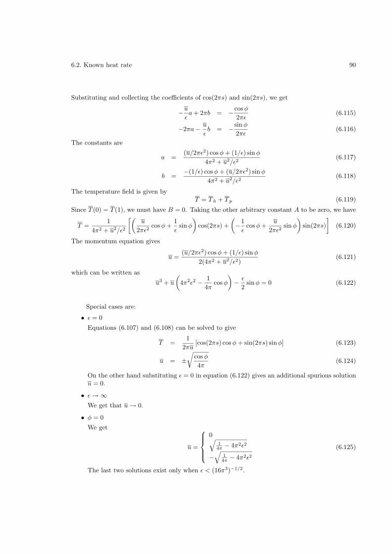
6.2. Known heat rate 90
Substituting and collecting the coefficients of cos(2πs) and sin(2πs), we get
−uǫa+ 2πb = −cosφ
2πǫ(6.115)
−2πa− u
ǫb = − sinφ
2πǫ(6.116)
The constants are
a =(u/2πǫ2) cosφ+ (1/ǫ) sinφ
4π2 + u2/ǫ2(6.117)
b =−(1/ǫ) cosφ+ (u/2πǫ2) sinφ
4π2 + u2/ǫ2(6.118)
The temperature field is given byT = Th + T p (6.119)
Since T (0) = T (1), we must have B = 0. Taking the other arbitrary constant A to be zero, we have
T =1
4π2 + u2/ǫ2
[(u
2πǫ2cosφ+
1
ǫsinφ
)cos(2πs) +
(−1
ǫcosφ+
u
2πǫ2sinφ
)sin(2πs)
](6.120)
The momentum equation gives
u =(u/2πǫ2) cosφ+ (1/ǫ) sinφ
2(4π2 + u2/ǫ2)(6.121)
which can be written as
u3 + u
(4π2ǫ2 − 1
4πcosφ
)− ǫ
2sinφ = 0 (6.122)
Special cases are:
• ǫ = 0
Equations (6.107) and (6.108) can be solved to give
T =1
2πu[cos(2πs) cosφ+ sin(2πs) sinφ] (6.123)
u = ±√
cosφ
4π(6.124)
On the other hand substituting ǫ = 0 in equation (6.122) gives an additional spurious solutionu = 0.
• ǫ→ ∞We get that u→ 0.
• φ = 0
We get
u =
0√14π − 4π2ǫ2
−√
14π − 4π2ǫ2
(6.125)
The last two solutions exist only when ǫ < (16π3)−1/2.
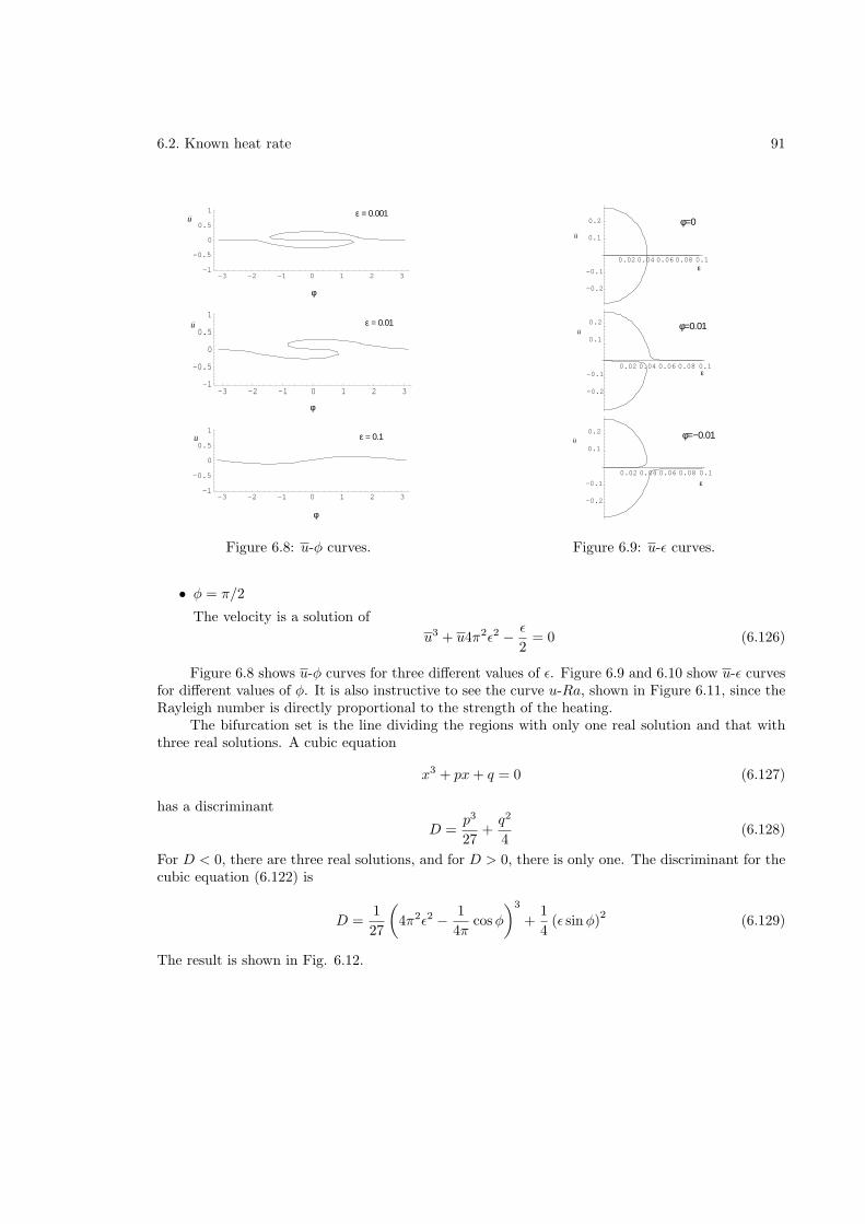
6.2. Known heat rate 91
-3 -2 -1 0 1 2 3-1
-0.5
0
0.5
1
-3 -2 -1 0 1 2 3-1
-0.5
0
0.5
1
φ
φ
-3 -2 -1 0 1 2 3-1
-0.5
0
0.5
1
φ
u
u
u
ε = 0.001
ε = 0.01
ε = 0.1
Figure 6.8: u-φ curves.
0.02 0.04 0.06 0.08 0.1
-0.2
-0.1
0.1
0.2
0.02 0.04 0.06 0.08 0.1
-0.2
-0.1
0.1
0.2
0.02 0.04 0.06 0.08 0.1
-0.2
-0.1
0.1
0.2
ε
ε
ε
u
u
u
φ=0
φ=0.01
φ=−0.01
Figure 6.9: u-ǫ curves.
• φ = π/2
The velocity is a solution of
u3 + u4π2ǫ2 − ǫ
2= 0 (6.126)
Figure 6.8 shows u-φ curves for three different values of ǫ. Figure 6.9 and 6.10 show u-ǫ curvesfor different values of φ. It is also instructive to see the curve u-Ra, shown in Figure 6.11, since theRayleigh number is directly proportional to the strength of the heating.
The bifurcation set is the line dividing the regions with only one real solution and that withthree real solutions. A cubic equation
x3 + px+ q = 0 (6.127)
has a discriminant
D =p3
27+q2
4(6.128)
For D < 0, there are three real solutions, and for D > 0, there is only one. The discriminant for thecubic equation (6.122) is
D =1
27
(4π2ǫ2 − 1
4πcosφ
)3
+1
4(ǫ sinφ)
2(6.129)
The result is shown in Fig. 6.12.
6.2. Known heat rate 92
0.02 0.04 0.06 0.08
-0.2
-0.1
0.1
0.2
0.02 0.04 0.06 0.08 0.1
0.05
0.1
0.15
0.2
0.02 0.04 0.06 0.08 0.1
0.02
0.04
0.06
0.08
0.1
φ=π/4
φ=π/4
φ=π/4
u
u
u
Figure 6.10: More u-ǫ curves.
10000 20000 30000 40000
-0.2
-0.1
0.1
0.2u
Ra
Figure 6.11: u-Ra for φ = 0.01 radians.
−100 −80 −60 −40 −20 0 20 40 60 80 1000
0.005
0.01
0.015
0.02
0.025
0.03
0.035
0.04
0.045
ε
φ (degrees)
Figure 6.12: Region with three solutions.
6.2. Known heat rate 93
6.2.4 Dynamic analysis
We rescale the nondimensional governing equations (6.56) and (6.57) by
u∗ =1
2πG1/2u (6.130)
T ∗ =1
2πG1/2T (6.131)
to get
du
dt+ u =
∫ 1
0
T g ds (6.132)
∂T
∂t+
1
2πu∂T
∂s= Gq +
G1/2K
2π
∂2T
∂s2(6.133)
where the hats and stars have been dropped.We take g = cos(2πs) and q = − sin(2πs− φ). Expanding the temperature in a Fourier series,
we get
T (s, t) = T0(t) +
∞∑
n=1
[T cn(t) cos(2πns) + T s
n(t) sin(2πns)] (6.134)
Substituting, we havedu
dt+ u =
1
2T c
1 (6.135)
and
dT0
dt+
∞∑
n=1
[dT c
n
dtcos(2πns) +
dT cn
dtsin(2πns)
]
+u∞∑
n=1
[−nT cn sin(2πns) + nT s
n cos(2πns)]
= −G [sin(2πs) cosφ− cos(2πs) sinφ]
−2πn2G1/2K∞∑
n=1
[T cn cos(2πns) + T s
n sin(2πns)] (6.136)
Integrating, we getdT0
dt= 0 (6.137)
Multiplying by cos(2πms) and integrating
1
2
dT cm
dt+m
2uT s
m =1
2G sinφ− πm2G1/2KT c
m (6.138)
Now multiplying by sin(2πms) and integrating
1
2
dT sm
dt− m
2uT c
m = −1
2G cosφ− πm2G1/2KT s
m (6.139)
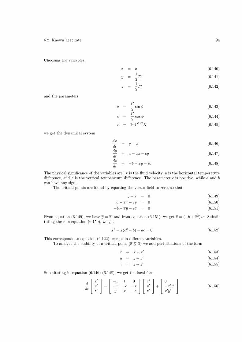
6.2. Known heat rate 94
Choosing the variables
x = u (6.140)
y =1
2T c
1 (6.141)
z =1
2T s
1 (6.142)
and the parameters
a =G
2sinφ (6.143)
b =G
2cosφ (6.144)
c = 2πG1/2K (6.145)
we get the dynamical system
dx
dt= y − x (6.146)
dy
dt= a− xz − cy (6.147)
dz
dt= −b+ xy − cz (6.148)
The physical significance of the variables are: x is the fluid velocity, y is the horizontal temperaturedifference, and z is the vertical temperature difference. The parameter c is positive, while a and bcan have any sign.
The critical points are found by equating the vector field to zero, so that
y − x = 0 (6.149)
a− xz − cy = 0 (6.150)
−b+ xy − cz = 0 (6.151)
From equation (6.149), we have y = x, and from equation (6.151), we get z = (−b+ x2)/c. Substi-tuting these in equation (6.150), we get
x3 + x(c2 − b) − ac = 0 (6.152)
This corresponds to equation (6.122), except in different variables.To analyze the stability of a critical point (x, y, z) we add perturbations of the form
x = x+ x′ (6.153)
y = y + y′ (6.154)
z = z + z′ (6.155)
Substituting in equation (6.146)-(6.148), we get the local form
d
dt
x′
y′
z′
=
−1 1 0−z −c −xy x −c
x′
y′
z′
+
0−x′z′x′y′
(6.156)
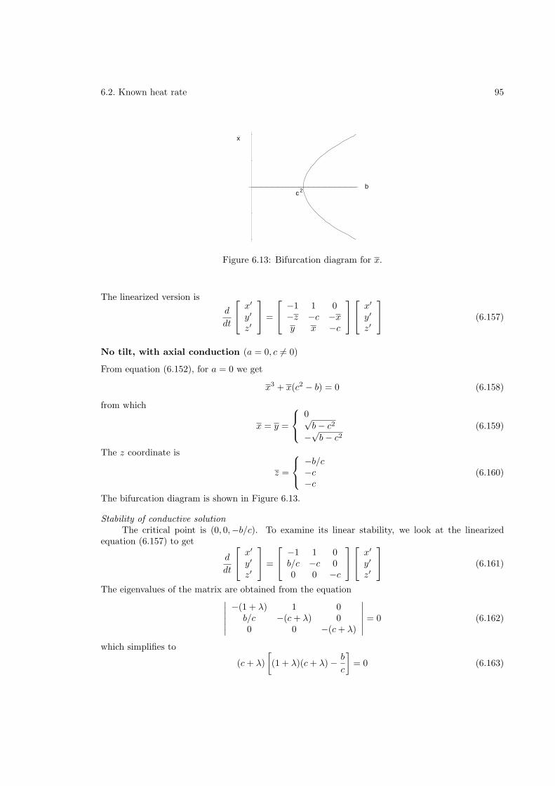
6.2. Known heat rate 95
b
x
c 2
Figure 6.13: Bifurcation diagram for x.
The linearized version is
d
dt
x′
y′
z′
=
−1 1 0−z −c −xy x −c
x′
y′
z′
(6.157)
No tilt, with axial conduction (a = 0, c 6= 0)
From equation (6.152), for a = 0 we get
x3 + x(c2 − b) = 0 (6.158)
from which
x = y =
0√b− c2
−√b− c2
(6.159)
The z coordinate is
z =
−b/c−c−c
(6.160)
The bifurcation diagram is shown in Figure 6.13.
Stability of conductive solutionThe critical point is (0, 0,−b/c). To examine its linear stability, we look at the linearized
equation (6.157) to get
d
dt
x′
y′
z′
=
−1 1 0b/c −c 00 0 −c
x′
y′
z′
(6.161)
The eigenvalues of the matrix are obtained from the equation∣∣∣∣∣∣
−(1 + λ) 1 0b/c −(c+ λ) 00 0 −(c+ λ)
∣∣∣∣∣∣= 0 (6.162)
which simplifies to
(c+ λ)
[(1 + λ)(c+ λ) − b
c
]= 0 (6.163)
6.2. Known heat rate 96
One eigenvalue isλ1 = −c (6.164)
Since c ≥ 0 this eigenvalue indicates stability. The other two are solutions of
λ2 + (c+ 1)λ+ (c− b
c) = 0 (6.165)
which are
λ2 =1
2
[−(c+ 1) −
√(c+ 1)2 − 4(c− b
c)
](6.166)
λ3 =1
2
[−(c+ 1) +
√(c+ 1)2 − 4(c− b
c)
](6.167)
λ2 is also negative and hence stable. λ3 is negative as long as
−(c+ 1) +
√(c+ 1)2 − 4(c− b
c) < 0 (6.168)
which givesb < c2 (6.169)
This is the condition for stability.In fact, one can also prove global stability of the conductive solution. Restoring the nonlinear
terms in equation (6.156) to equation (6.161), we have
dx′
dt= y′ − x′ (6.170)
dy′
dt=
b
cx′ − cy′ − x′z′ (6.171)
dz′
dt= −cz′ + x′y′ (6.172)
Let
E(x, y, z) =b
cx′2 + y′2 + z′2 (6.173)
Thus
1
2
dE
dt=
b
cx′dx′
dt+ y′
dy′
dt+ z′
dz′
dt(6.174)
= −bcx′2 +
2b
cx′y′ − cy′2 − cz′2 (6.175)
= −bc(x′ − y′)2 − (c− b
c)y′2 − cz′2 (6.176)
Since
E ≥ 0 (6.177)
dE
dt≤ 0 (6.178)
6.2. Known heat rate 97
for 0 ≤ b ≤ c2, E is a Liapunov function, and the critical point is stable to all perturbations in thisregion. The bifurcation at b = c2 is thus supercritical.
Stability of convective solutionFor b > c2, only one critical point (
√b− c2,
√b− c2,−c) will be considered, the other being
similar. We use the linearized equations (6.157). Its eigenvalues are solutions of
∣∣∣∣∣∣
−(1 + λ) 1 0
c −(c+ λ) −√b− c2√
b− c2√b− c2 −(c+ λ)
∣∣∣∣∣∣= 0 (6.179)
This can be expanded to give
λ3 + λ2(1 + 2c) + λ(b+ c) + 2(b− c2) = 0 (6.180)
The Hurwitz criteria for stability require that all coefficients be positive, which they are. Also thedeterminants
D1 = 1 + 2c (6.181)
D2 =
∣∣∣∣1 + 2c 2(b− c2)
1 b+ c
∣∣∣∣ (6.182)
D3 =
∣∣∣∣∣∣
1 + 2c 2(b− c2) 01 b+ c 00 1 + 2c 2(b− c2)
∣∣∣∣∣∣(6.183)
should be positive. This requires that
b <c(1 + 4c)
1 − 2cif c < 1/2 (6.184)
b >c(1 + 4c)
1 − 2cif c > 1/2 (6.185)
(6.186)
With tilt, no axial conduction (a 6= 0, c = 0)
The dynamical system (6.146)-(6.148) simplifies to
dx
dt= y − x (6.187)
dy
dt= a− xz (6.188)
dz
dt= −b+ xy (6.189)
The critical points are ±(√b,√b, a/
√b). The linear stability of the point P+ given by (
√b,√b, a/
√b)
will be analyzed. From equation (6.157), the solutions of
∣∣∣∣∣∣
−(1 + λ) 1 0
−a/√b −λ −
√b√
b√b −λ
∣∣∣∣∣∣= 0 (6.190)
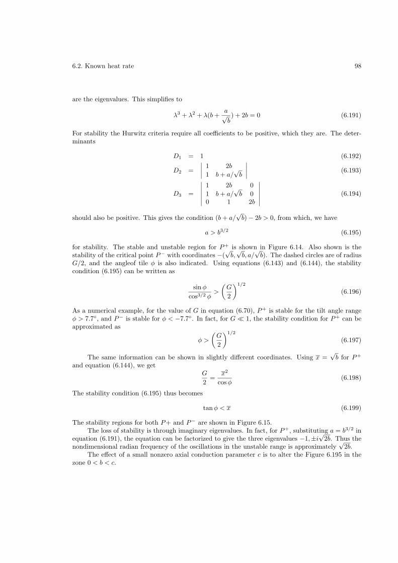
6.2. Known heat rate 98
are the eigenvalues. This simplifies to
λ3 + λ2 + λ(b+a√b) + 2b = 0 (6.191)
For stability the Hurwitz criteria require all coefficients to be positive, which they are. The deter-minants
D1 = 1 (6.192)
D2 =
∣∣∣∣1 2b
1 b+ a/√b
∣∣∣∣ (6.193)
D3 =
∣∣∣∣∣∣
1 2b 0
1 b+ a/√b 0
0 1 2b
∣∣∣∣∣∣(6.194)
should also be positive. This gives the condition (b+ a/√b) − 2b > 0, from which, we have
a > b3/2 (6.195)
for stability. The stable and unstable region for P+ is shown in Figure 6.14. Also shown is thestability of the critical point P− with coordinates −(
√b,√b, a/
√b). The dashed circles are of radius
G/2, and the angleof tile φ is also indicated. Using equations (6.143) and (6.144), the stabilitycondition (6.195) can be written as
sinφ
cos3/2 φ>
(G
2
)1/2
(6.196)
As a numerical example, for the value of G in equation (6.70), P+ is stable for the tilt angle rangeφ > 7.7, and P− is stable for φ < −7.7. In fact, for G≪ 1, the stability condition for P+ can beapproximated as
φ >
(G
2
)1/2
(6.197)
The same information can be shown in slightly different coordinates. Using x =√b for P+
and equation (6.144), we getG
2=
x2
cosφ(6.198)
The stability condition (6.195) thus becomes
tanφ < x (6.199)
The stability regions for both P+ and P− are shown in Figure 6.15.The loss of stability is through imaginary eigenvalues. In fact, for P+, substituting a = b3/2 in
equation (6.191), the equation can be factorized to give the three eigenvalues −1,±i√
2b. Thus thenondimensional radian frequency of the oscillations in the unstable range is approximately
√2b.
The effect of a small nonzero axial conduction parameter c is to alter the Figure 6.195 in thezone 0 < b < c.
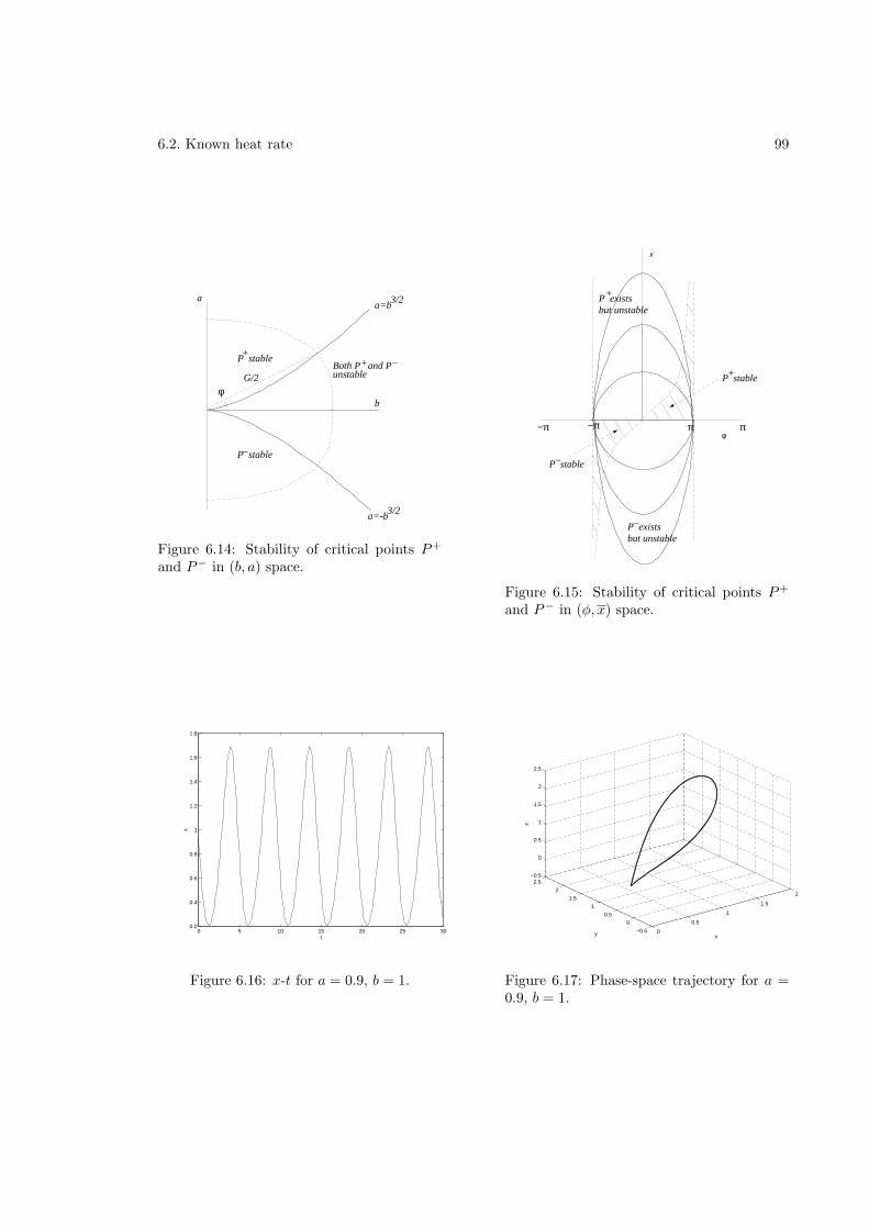
6.2. Known heat rate 99
a
b
a=b3/2
P stableBoth P and Punstable
+
P stable_
+ _
a=-b3/2
G/2
φ
Figure 6.14: Stability of critical points P+
and P− in (b, a) space.
π π−π −π
x
φ
P stable
P stable
+
_
P existsbut unstable
+
P existsbut unstable
_
Figure 6.15: Stability of critical points P+
and P− in (φ, x) space.
0 5 10 15 20 25 300.2
0.4
0.6
0.8
1
1.2
1.4
1.6
1.8
t
x
Figure 6.16: x-t for a = 0.9, b = 1.
0
0.5
1
1.5
2
−0.5
0
0.5
1
1.5
2
2.5−0.5
0
0.5
1
1.5
2
2.5
xy
z
Figure 6.17: Phase-space trajectory for a =0.9, b = 1.
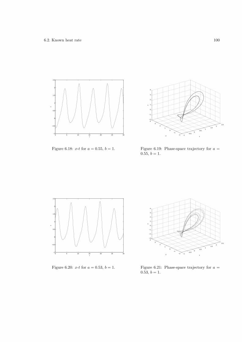
6.2. Known heat rate 100
0 5 10 15 20 25 30−1
−0.5
0
0.5
1
1.5
2
2.5
t
x
Figure 6.18: x-t for a = 0.55, b = 1.
−1−0.5
00.5
11.5
22.5
−2
−1
0
1
2
3
4−2
−1
0
1
2
3
4
xy
zFigure 6.19: Phase-space trajectory for a =0.55, b = 1.
0 5 10 15 20 25 30−1
−0.5
0
0.5
1
1.5
2
2.5
t
x
Figure 6.20: x-t for a = 0.53, b = 1.
−1−0.5
00.5
11.5
22.5
−2
−1
0
1
2
3
4−3
−2
−1
0
1
2
3
4
xy
z
Figure 6.21: Phase-space trajectory for a =0.53, b = 1.
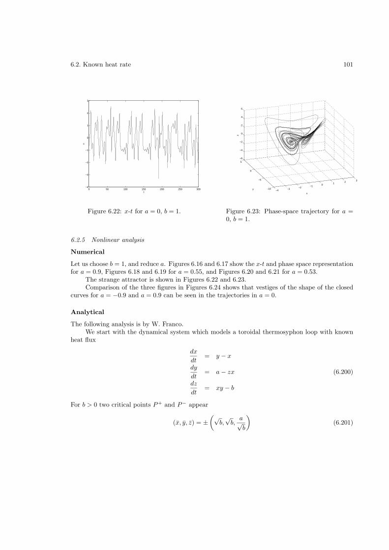
6.2. Known heat rate 101
0 50 100 150 200 250 300−4
−3
−2
−1
0
1
2
3
t
x
Figure 6.22: x-t for a = 0, b = 1.
−4 −3 −2 −1 0 1 2 3
−10
−5
0
5
−6
−4
−2
0
2
4
6
x
y
z
Figure 6.23: Phase-space trajectory for a =0, b = 1.
6.2.5 Nonlinear analysis
Numerical
Let us choose b = 1, and reduce a. Figures 6.16 and 6.17 show the x-t and phase space representationfor a = 0.9, Figures 6.18 and 6.19 for a = 0.55, and Figures 6.20 and 6.21 for a = 0.53.
The strange attractor is shown in Figures 6.22 and 6.23.Comparison of the three figures in Figures 6.24 shows that vestiges of the shape of the closed
curves for a = −0.9 and a = 0.9 can be seen in the trajectories in a = 0.
Analytical
The following analysis is by W. Franco.We start with the dynamical system which models a toroidal thermosyphon loop with known
heat flux
dx
dt= y − x
dy
dt= a− zx (6.200)
dz
dt= xy − b
For b > 0 two critical points P+ and P− appear
(x, y, z) = ±(√
b,√b,
a√b
)(6.201)
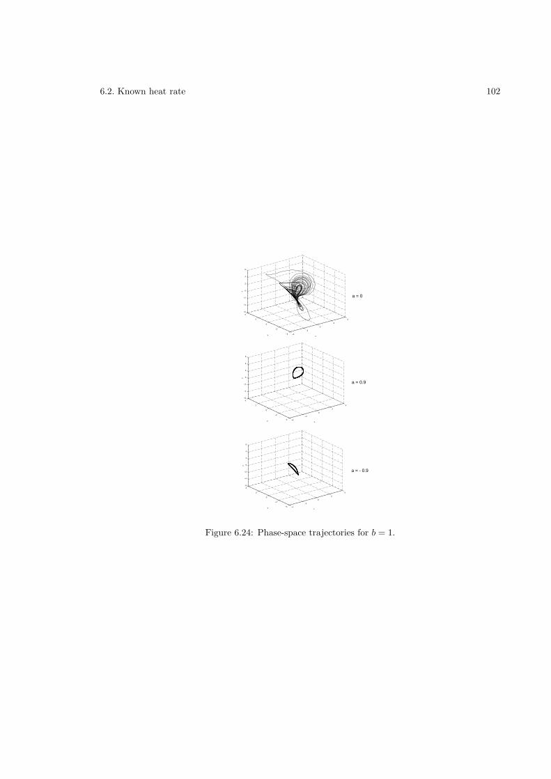
6.2. Known heat rate 102
−4
−2
0
2
4
−4
−2
0
2
4−6
−4
−2
0
2
4
6
xy
z
−4
−2
0
2
4
−4
−2
0
2
4−6
−4
−2
0
2
4
6
xy
z
−4
−2
0
2
4
−4
−2
0
2
4−6
−4
−2
0
2
4
6
xy
z
a = 0
a = 0.9
a = - 0.9
Figure 6.24: Phase-space trajectories for b = 1.
6.2. Known heat rate 103
The local form respect to P+ is
dx′
dt= y′ − x′
dy′
dt= − a√
bx′ −
√bz′ (6.202)
dz′
dt=
√bx′ +
√by′
For stability a > b32 . At a = b
32 the eigenvalues are −1,±
√2bi, thus a nonlinear analysis through
the center manifold projection is possible. Let’s introduce a perturbation of the form a = b32 + ǫ and
the following change of variables
α =a√b
β =√b
rewriting the local form, dropping the primes and regarding the perturbation the system becomes
dx
dt= y − x
dy
dt=
(β2 +
ǫ
β
)x− βz (6.203)
dz
dt= βx− βy
for stability α > β2.Let’s apply the following transformation:
x = w1 +2
2β2 + 1w2 +
2β√
2
2β2 + 1
y = 2w2 (6.204)
z = −βw1 −2β
2β2 + 1w2 +
2√
2(β2 + 1
)
2β2 + 1w3
in the new variables
w =
−1 0 0
0 0 −√
2β
0√
2β 0
w + Pw + l(w) (6.205)
The center manifold projection is convenient to use if the large-time dynamic behavior is ofinterest. In many dimensional systems, the system often settles into the same large-time dynamicsirrespective of the initial condition; this is usually less complex than the initial dynamics and canbe described by far simple evolution equations.
We first state the definition of an invariant manifold for the equation
x = N(x) (6.206)
where x ∈ Rn. A set S ⊂ Rn is a local invariant manifold for (6.206) if for x0 ⊂ S, the solution x(t)of (6.206) is in S for | t |< T where T > 0. If we can always choose T = ∞, then S is an invariant
6.2. Known heat rate 104
manifold. Consider the system
x = Ax+ f(x, y)
y = By + g(x, y) (6.207)
where x ∈ Rn, y ∈ Rm and A and B are constant matrices such that all the eigenvalues of A havezero real parts while all the eigenvalues of B have negative real parts. If y = h(x) is an invariantmanifold for (6.207) and h is smooth, then it is called a center manifold if h(0) = 0,h′(0) = 0. Theflow on the center manifold is governed by the n-dimensional system
x = Ax+ f(x, h(x)) (6.208)
The last equation contains all the necessary information needed to determine the asymptotic behaviorof small solutions of (6.207).
Now we calculate, or at least approximate the center manifold h(w). Substituting w1 =h(w2, w3) in the first component of (6.205) and using the chain rule, we obtain
w1 =
(∂h
∂w2,∂h
∂w3
)
w2
w3
= −h+ l1 (w2, w3, h) (6.209)
We seek a center manifoldh = aw2
2 + bw2w3 + cw23 +O(3) (6.210)
substituting in (6.209)
(2aw2 + bw3, 2cw3 + bw2)
−√
2βw3
√2βw2
=
−(aw2
2 + bw2w3 + cw23
)+
(k1w
22 + k2w2w3 + k3w
23
)+O(3)
Equating powers of x2,xy and y2, we find that
a = k1 − b√
2β
c = k3 + b√
2β
b =k2 + 2
√2β (k1 − k3)
8β2 + 1
The reduced system is therefore given by
w2 = −√
2βw3 + s2 (w2, w3)
w3 =√
2βw2 + s3 (w2, w3) (6.211)
Normal form: Now we carry out a smooth nonlinear coordinate transform of the type
w = v + ψ(v) (6.212)
to simplify (6.211) by transforming away many nonlinear terms. The system in the new coordinatesis
v =
(0 −
√2β√
2β 0
)+
(νv1 − γv2)(v21 + v2
2
)
(νv2 + γv1)(v21 + v2
2
)
(6.213)
6.2. Known heat rate 105
where ν and γ depend on the nonlinear part of (6.211). This is the unfolding of the Hopf bifurcation.Although the normal form theory presented in class pertains to a Jacobian whose eigenvalues
all lie on the imaginary axis, one can also present a perturbed version. The eigenvalues are thenclose to the imaginary axis but not quite on it. Consider the system
v = Av + Av + f(v) (6.214)
where the Jacobian A has been evaluated at a point in the parameter space where all its eigenvaluesare on the imaginary axis, A represents a linear expansion of order µ in the parameters above thatpoint; a perturbed Jacobian. The perturbation parameter represents the size of the neighborhood inthe parameter space. We stipulate the order of µ such that the real part of the eigenvalues of A + A
is such that, to leading order, A does not change the coefficients of the leading order nonlinear termsof the transformed equation. The linear part A + A of perturbed Hopf can always be transformedto (
µ −ωω µ
)
The required transformation is a near identity linear transformation
v = u + Bu
such that the linear part of (6.214) is transformed to
u =(A + AB − BA + A
)z
For the Hopf bifurcation if
A =
(a1 a2
a3 a4
)
then
µ =a1 + a4
ω
Therefore for ǫ small we can write (6.213) as
v =
(0 −
√2β√
2β 0
)v +
(p22 p23
p32 p33
)v +
f1(v)
f2(v)
(6.215)
where the perturbation matrix comes from (6.205). Applying a near identity transformation of theform v = u + Bu the system becomes
u =
(µ −
√2β√
2β µ
)u +
(νu1 − γu2)(u2
1 + u22
)
(νu2 + γu1)(u2
1 + u22
)
(6.216)
which is the unfolding for the perturbed Hopf bifurcation. In polar coordinates we have
r = µr + νr3
θ =√
2β (6.217)
where
µ = − ǫ√
2
2β2 (2β2 + 1)(6.218)
6.3. Known wall temperature 106
ν = −40β6 + 40β4 + 12β3 + 10β2 + 12β + 3
4 (8β2 + 1) (2β2 + 1)4 (6.219)
Appendix
k1 = −8β(β2 + 1
)
(2β2 + 1)3
k2 =
(β2 + 1
) (4√
2 − 8√
2β2)
(2β2 + 1)3 (6.220)
k3 =8β(β2 + 1
)
(2β2 + 1)3
p22 = − ǫ
β (2β2 + 1)
p23 = − ǫ√
2
2β2 + 1(6.221)
From the literature
ν =1
16(fxxx + fxyy + gxxy + gyyy)
+1
16ω(fxy(fxx + fyy) − gxy(gxx − gyy) − fxxgxx − fyygyy) (6.222)
in our problem f = f1, g = f2, x = v1, y = v2 and ω =√
2β.
6.3 Known wall temperature
The heating is now convective with a heat transfer coefficient U , and an external temperature ofTw(s). Thus,
q = PU(T − Tw) (6.223)
Neglecting axial conduction
Pα
ρ0Au =
β
L
∫ L
0
T (s)g(s) ds (6.224)
udT
ds= γ
[T − Tw(s)
](6.225)
where γ = UP/ρ0Acp1. Multiplying the second equation by e−γs/u/u, we get
d
ds
(e−γs/uT
)= −γ
ue−γs/uTw (6.226)
Integrating, we get
T = eγs/u
[−γu
∫ s
0
e−γs′/uTw(s′) ds′ + T0
](6.227)
1The sign of γ appears to be wrong.
6.4. Mixed condition 107
Since T (L) = T (0), we get
T0 =γ
u
eγL/u∫ L
0e−γs′/uTw(s′) ds′
eγL/u − 1(6.228)
The velocity is obtained from
Pα
ρ0Au =
β
L
∫ L
0
[eγs/u
−γu
∫ s
0
e−γs′/uTw(s′) ds′ + T0
]g(s) ds (6.229)
This is a transcendental equation that may have more than one real solution.
Example 6.3Show that there is no motion if the wall temperature is uniform.
Take Tw to be a constant. Then equation (6.225) can be written as
d(T − Tw)
T − Tw
=γ
uds (6.230)
The solution to this isT = Tw + K eγs/u (6.231)
where K is a constant. Continuity of T at s = 0 and s = L gives K = 0. Hence T = Tw, and, from equation(6.224), u = 0.
Assume the wall temperature to be
Tw(s) = − sin(2πs− φ) (6.232)
The temperature field is
T =b
r2 − r1
(cos(2πs− φ)
2π(1 + r22/4π2)
)−(
cos(2πs− φ)
2π(1 + r162/4π2)
)(6.233)
6.4 Mixed condition
The following has been written by A. Pacheco-Vega.It is common, especially in experiments, to have one part of the loop heated with a known heat
rate and the rest with known wall temperature. Thus for part of the loop the wall temperature isknown so that q = PU(T − Tw(s)), while q(s) is known for the rest. As an example, consider
q =
PU(T − T0) for φ
2π ≤ s ≤ π + φ2π
q0 for π + φ2π < s < 2π + φ
2π
(6.234)
where T0 and q0 are constants.
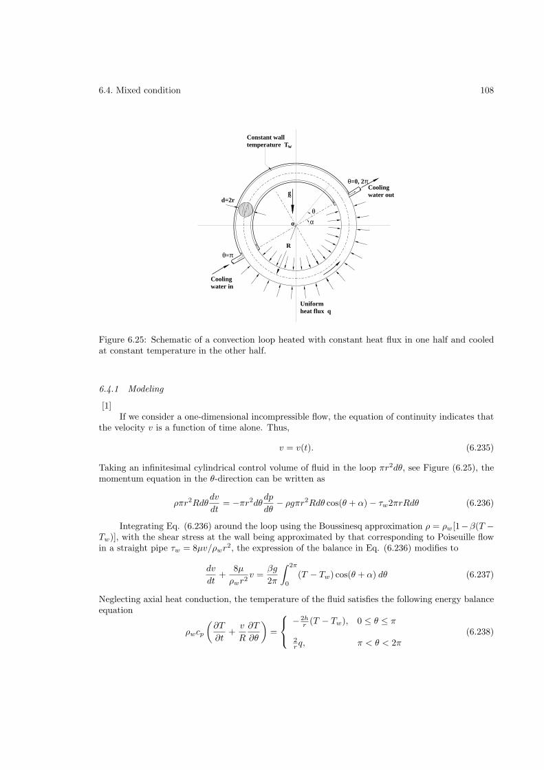
6.4. Mixed condition 108
Coolingwater out
Coolingwater in
d=2r
R
θ
α
θ=0, 2π
θ=π
g~
Uniformheat flux q
Constant walltemperature Tw
o
Figure 6.25: Schematic of a convection loop heated with constant heat flux in one half and cooledat constant temperature in the other half.
6.4.1 Modeling
[1]If we consider a one-dimensional incompressible flow, the equation of continuity indicates that
the velocity v is a function of time alone. Thus,
v = v(t). (6.235)
Taking an infinitesimal cylindrical control volume of fluid in the loop πr2dθ, see Figure (6.25), themomentum equation in the θ-direction can be written as
ρπr2Rdθdv
dt= −πr2dθdp
dθ− ρgπr2Rdθ cos(θ + α) − τw2πrRdθ (6.236)
Integrating Eq. (6.236) around the loop using the Boussinesq approximation ρ = ρw[1−β(T −Tw)], with the shear stress at the wall being approximated by that corresponding to Poiseuille flowin a straight pipe τw = 8µv/ρwr
2, the expression of the balance in Eq. (6.236) modifies to
dv
dt+
8µ
ρwr2v =
βg
2π
∫ 2π
0
(T − Tw) cos(θ + α) dθ (6.237)
Neglecting axial heat conduction, the temperature of the fluid satisfies the following energy balanceequation
ρwcp
(∂T
∂t+v
R
∂T
∂θ
)=
− 2hr (T − Tw), 0 ≤ θ ≤ π
2r q, π < θ < 2π
(6.238)
6.4. Mixed condition 109
Following the notation used by Greif et al. (1979), the nondimensional time, velocity and tempera-ture are defined as
τ =t
2πR/V, w =
v
V, φ =
T − Tw
q/h(6.239)
respectively, where
V =
(gβRrq
2πcpµ
)1/2
. (6.240)
Accordingly, Eqs. (6.237) and (6.238) become
dw
dτ+ Γw =
πΓ
4D
∫ 2π
0
φ cos(θ + α) dθ (6.241)
and∂φ
∂τ+ 2πw
∂φ
∂θ=
−2Dφ, 0 ≤ θ ≤ π2D, π < θ < 2π
(6.242)
where the parameters D and Γ are defined by
D =2πRh
ρwcprVΓ =
16πµR
ρwr2V(6.243)
6.4.2 Steady State
The steady-state governing equations without axial conduction are
w =π
4D
∫ 2π
0
φ cos(θ + α) dθ (6.244)
and
dφ
dθ=
− Dπw φ, 0 ≤ θ ≤ π
Dπw , π < θ < 2π
(6.245)
where w and φ are the steady-state values of velocity and temperature respectively. Eq. (6.245) canbe integrated to give
φ(θ) =
A e−(Dθ/πw), 0 ≤ θ ≤ π
Dπw θ +B, π < θ < 2π
(6.246)
Applying the condition of continuity in the temperature, such that φ(0) = φ(2π) and φ(π−) = φ(π+)the constants A and B can be determined. These are
A =D
w
1
1 − e(−D/w)B =
D
w
[2 e(−D/w) − 1
1 − e(−D/w)
](6.247)
The resulting temperature filed is
φ(θ) =
Dw
e−(Dθ/πw)
1−e−(D/w) , 0 ≤ θ ≤ π
Dw
[θπ + 2e−(D/w)
−11−e−(D/w)
], π < θ < 2π
(6.248)
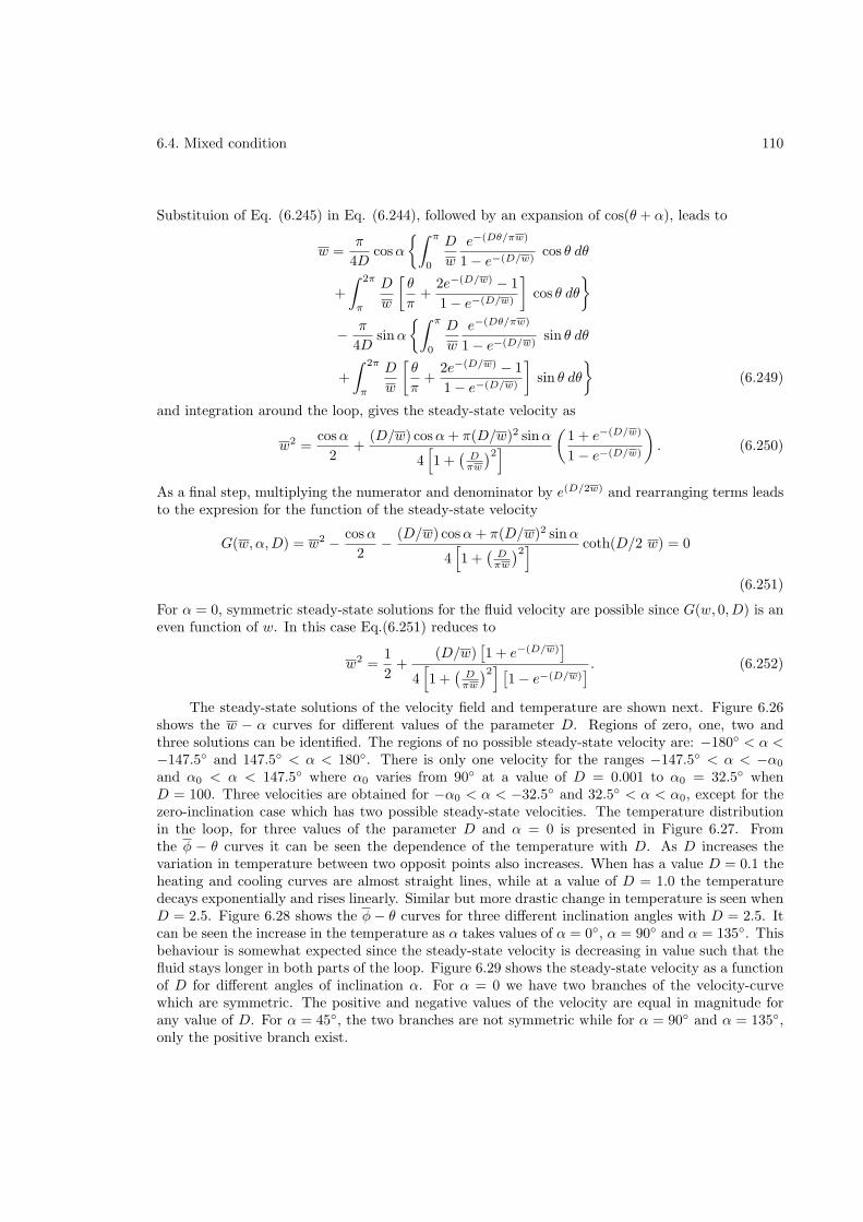
6.4. Mixed condition 110
Substituion of Eq. (6.245) in Eq. (6.244), followed by an expansion of cos(θ + α), leads to
w =π
4Dcosα
∫ π
0
D
w
e−(Dθ/πw)
1 − e−(D/w)cos θ dθ
+
∫ 2π
π
D
w
[θ
π+
2e−(D/w) − 1
1 − e−(D/w)
]cos θ dθ
− π
4Dsinα
∫ π
0
D
w
e−(Dθ/πw)
1 − e−(D/w)sin θ dθ
+
∫ 2π
π
D
w
[θ
π+
2e−(D/w) − 1
1 − e−(D/w)
]sin θ dθ
(6.249)
and integration around the loop, gives the steady-state velocity as
w2 =cosα
2+
(D/w) cosα+ π(D/w)2 sinα
4[1 +
(Dπw
)2](
1 + e−(D/w)
1 − e−(D/w)
). (6.250)
As a final step, multiplying the numerator and denominator by e(D/2w) and rearranging terms leadsto the expresion for the function of the steady-state velocity
G(w,α,D) = w2 − cosα
2− (D/w) cosα+ π(D/w)2 sinα
4[1 +
(Dπw
)2] coth(D/2 w) = 0
(6.251)
For α = 0, symmetric steady-state solutions for the fluid velocity are possible since G(w, 0,D) is aneven function of w. In this case Eq.(6.251) reduces to
w2 =1
2+
(D/w)[1 + e−(D/w)
]
4[1 +
(Dπw
)2] [1 − e−(D/w)
] . (6.252)
The steady-state solutions of the velocity field and temperature are shown next. Figure 6.26shows the w − α curves for different values of the parameter D. Regions of zero, one, two andthree solutions can be identified. The regions of no possible steady-state velocity are: −180 < α <−147.5 and 147.5 < α < 180. There is only one velocity for the ranges −147.5 < α < −α0
and α0 < α < 147.5 where α0 varies from 90 at a value of D = 0.001 to α0 = 32.5 whenD = 100. Three velocities are obtained for −α0 < α < −32.5 and 32.5 < α < α0, except for thezero-inclination case which has two possible steady-state velocities. The temperature distributionin the loop, for three values of the parameter D and α = 0 is presented in Figure 6.27. Fromthe φ − θ curves it can be seen the dependence of the temperature with D. As D increases thevariation in temperature between two opposit points also increases. When has a value D = 0.1 theheating and cooling curves are almost straight lines, while at a value of D = 1.0 the temperaturedecays exponentially and rises linearly. Similar but more drastic change in temperature is seen whenD = 2.5. Figure 6.28 shows the φ− θ curves for three different inclination angles with D = 2.5. Itcan be seen the increase in the temperature as α takes values of α = 0, α = 90 and α = 135. Thisbehaviour is somewhat expected since the steady-state velocity is decreasing in value such that thefluid stays longer in both parts of the loop. Figure 6.29 shows the steady-state velocity as a functionof D for different angles of inclination α. For α = 0 we have two branches of the velocity-curvewhich are symmetric. The positive and negative values of the velocity are equal in magnitude forany value of D. For α = 45, the two branches are not symmetric while for α = 90 and α = 135,only the positive branch exist.
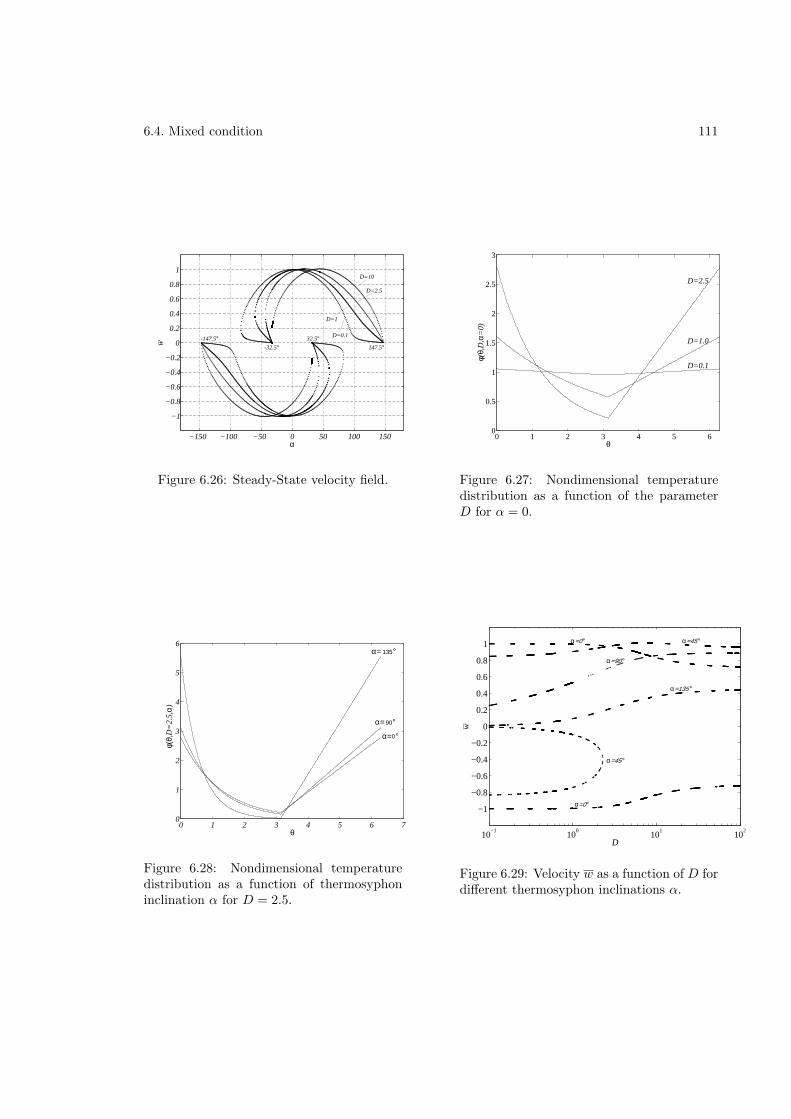
6.4. Mixed condition 111
−150 −100 −50 0 50 100 150
−1
−0.8
−0.6
−0.4
−0.2
0
0.2
0.4
0.6
0.8
1
α
w
D=0.1
D=1
D=2.5
D=10
147.5°-147.5°
-32.5°32.5°
Figure 6.26: Steady-State velocity field.
0 1 2 3 4 5 60
0.5
1
1.5
2
2.5
3
θ
φ(θ,
D,α
=0
)
D=0.1
D=1.0
D=2.5
Figure 6.27: Nondimensional temperaturedistribution as a function of the parameterD for α = 0.
0 1 2 3 4 5 6 70
1
2
3
4
5
6
θ
α= °
α= °
α= °
φ(θ,
D=
2.5
,α)
0
90
135
Figure 6.28: Nondimensional temperaturedistribution as a function of thermosyphoninclination α for D = 2.5.
102
α=45 °
100
101
D10
−1
−1
−0.8
−0.6
−0.4
−0.2
0
0.2
0.4
0.6
0.8
1
w
α=45 °
α=0°
α=135 °
α=90 °
α=0°
Figure 6.29: Velocity w as a function of D fordifferent thermosyphon inclinations α.
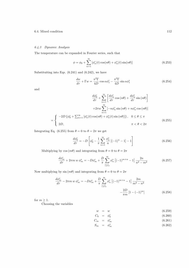
6.4. Mixed condition 112
6.4.3 Dynamic Analysis
The temperature can be expanded in Fourier series, such that
φ = φ0 +
∞∑
n=1
[φcn(t) cos(nθ) + φs
n(t) sin(nθ)] (6.253)
Substituiting into Eqs. (6.241) and (6.242), we have
dw
dτ+ Γw =
π2Γ
4Dcosαφc
1 −π2Γ
4Dsinαφs
1 (6.254)
and
dφc0
dτ+
∞∑
n=1
[dφc
n
dτcos (nθ) +
dφsn
dτsin (nθ)
]
+2πw
∞∑
n=1
[−nφcn sin (nθ) + nφs
n cos (nθ)]
=
−2D φc0 +
∑∞
n=1 [φcn(t) cos(nθ) + φs
n(t) sin (nθ)] , 0 ≤ θ ≤ π
2D, π < θ < 2π(6.255)
Integrating Eq. (6.255) from θ = 0 to θ = 2π we get
dφc0
dτ= −D
[φc
0 −1
π
∞∑
n=1
φsn
n[(−1)n − 1] − 1
](6.256)
Multiplying by cos (mθ) and integrating from θ = 0 to θ = 2π
dφcm
dτ+ 2πm w φs
m = −Dφcm +
D
π
∞∑
n=1n 6=m
φsn
[(−1)m+n − 1
] 2n
n2 −m2(6.257)
Now multiplying by sin (mθ) and integrating from θ = 0 to θ = 2π
dφsm
dτ− 2πm w φc
m = −Dφsm +
D
π
∞∑
n=0n 6=m
φcn
[(−1)m+n − 1
] 2m
m2 − n2
− 2D
πm[1 − (−1)m] (6.258)
for m ≥ 1.Choosing the variables
w = w (6.259)
C0 = φc0 (6.260)
Cm = φcm (6.261)
Sm = φsm (6.262)
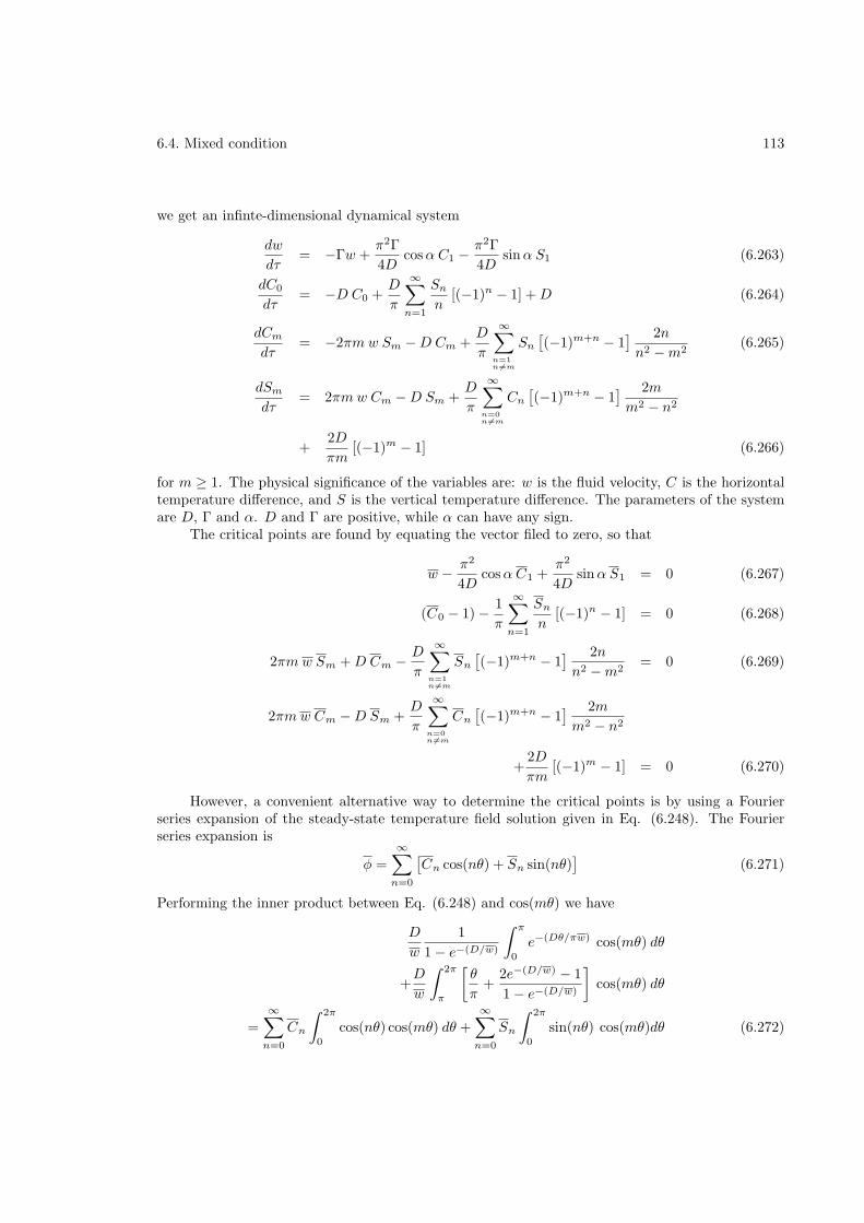
6.4. Mixed condition 113
we get an infinte-dimensional dynamical system
dw
dτ= −Γw +
π2Γ
4Dcosα C1 −
π2Γ
4Dsinα S1 (6.263)
dC0
dτ= −D C0 +
D
π
∞∑
n=1
Sn
n[(−1)n − 1] +D (6.264)
dCm
dτ= −2πm w Sm −D Cm +
D
π
∞∑
n=1n 6=m
Sn
[(−1)m+n − 1
] 2n
n2 −m2(6.265)
dSm
dτ= 2πm w Cm −D Sm +
D
π
∞∑
n=0n 6=m
Cn
[(−1)m+n − 1
] 2m
m2 − n2
+2D
πm[(−1)m − 1] (6.266)
for m ≥ 1. The physical significance of the variables are: w is the fluid velocity, C is the horizontaltemperature difference, and S is the vertical temperature difference. The parameters of the systemare D, Γ and α. D and Γ are positive, while α can have any sign.
The critical points are found by equating the vector filed to zero, so that
w − π2
4Dcosα C1 +
π2
4Dsinα S1 = 0 (6.267)
(C0 − 1) − 1
π
∞∑
n=1
Sn
n[(−1)n − 1] = 0 (6.268)
2πm w Sm +D Cm − D
π
∞∑
n=1n 6=m
Sn
[(−1)m+n − 1
] 2n
n2 −m2= 0 (6.269)
2πm w Cm −D Sm +D
π
∞∑
n=0n 6=m
Cn
[(−1)m+n − 1
] 2m
m2 − n2
+2D
πm[(−1)m − 1] = 0 (6.270)
However, a convenient alternative way to determine the critical points is by using a Fourierseries expansion of the steady-state temperature field solution given in Eq. (6.248). The Fourierseries expansion is
φ =
∞∑
n=0
[Cn cos(nθ) + Sn sin(nθ)
](6.271)
Performing the inner product between Eq. (6.248) and cos(mθ) we have
D
w
1
1 − e−(D/w)
∫ π
0
e−(Dθ/πw) cos(mθ) dθ
+D
w
∫ 2π
π
[θ
π+
2e−(D/w) − 1
1 − e−(D/w)
]cos(mθ) dθ
=
∞∑
n=0
Cn
∫ 2π
0
cos(nθ) cos(mθ) dθ +
∞∑
n=0
Sn
∫ 2π
0
sin(nθ) cos(mθ)dθ (6.272)
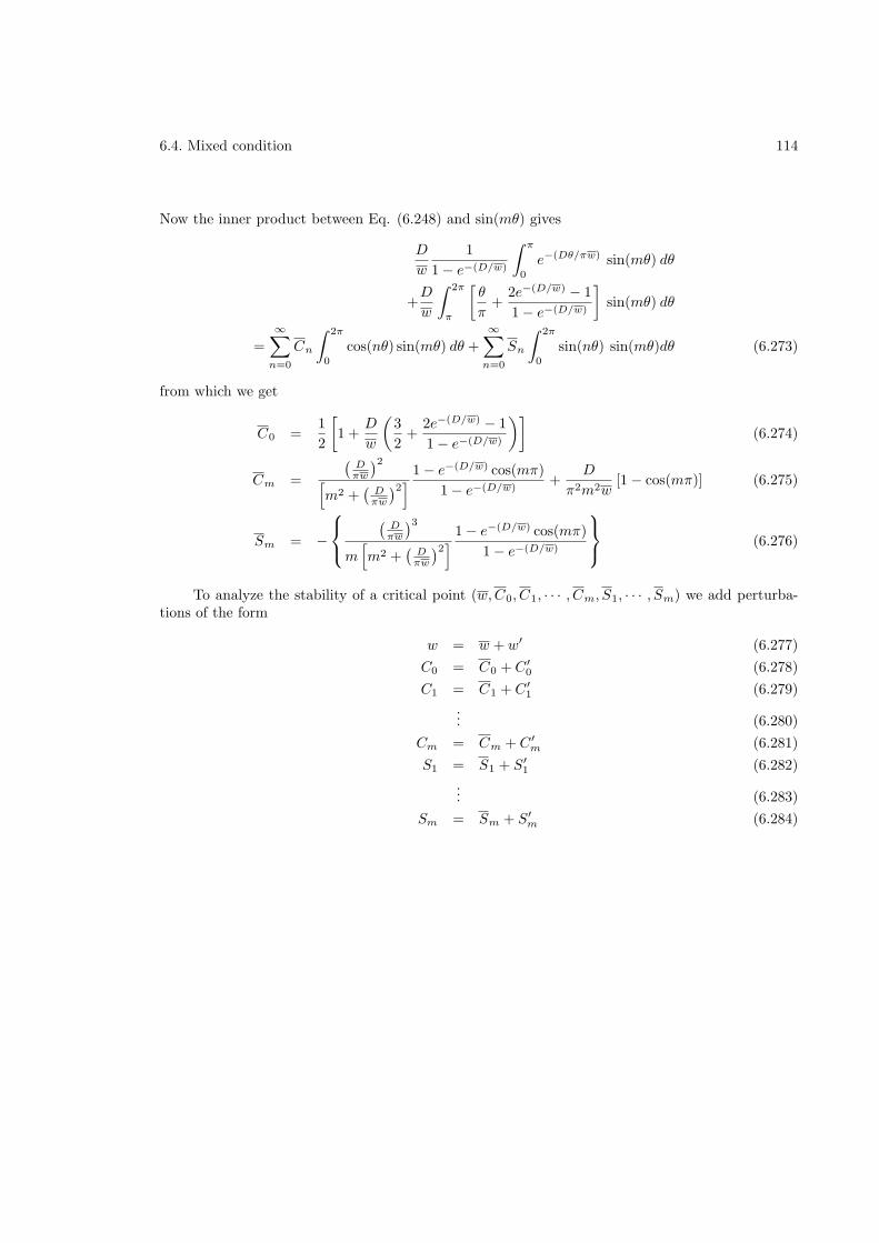
6.4. Mixed condition 114
Now the inner product between Eq. (6.248) and sin(mθ) gives
D
w
1
1 − e−(D/w)
∫ π
0
e−(Dθ/πw) sin(mθ) dθ
+D
w
∫ 2π
π
[θ
π+
2e−(D/w) − 1
1 − e−(D/w)
]sin(mθ) dθ
=
∞∑
n=0
Cn
∫ 2π
0
cos(nθ) sin(mθ) dθ +
∞∑
n=0
Sn
∫ 2π
0
sin(nθ) sin(mθ)dθ (6.273)
from which we get
C0 =1
2
[1 +
D
w
(3
2+
2e−(D/w) − 1
1 − e−(D/w)
)](6.274)
Cm =
(Dπw
)2[m2 +
(Dπw
)2]1 − e−(D/w) cos(mπ)
1 − e−(D/w)+
D
π2m2w[1 − cos(mπ)] (6.275)
Sm = −
(Dπw
)3
m[m2 +
(Dπw
)2]1 − e−(D/w) cos(mπ)
1 − e−(D/w)
(6.276)
To analyze the stability of a critical point (w,C0, C1, · · · , Cm, S1, · · · , Sm) we add perturba-tions of the form
w = w + w′ (6.277)
C0 = C0 + C ′
0 (6.278)
C1 = C1 + C ′
1 (6.279)
... (6.280)
Cm = Cm + C ′
m (6.281)
S1 = S1 + S′
1 (6.282)
... (6.283)
Sm = Sm + S′
m (6.284)
6.4. Mixed condition 115
Substituting in Eqs. (6.263) to (6.266), we obtain the local form
dw′
dτ= −Γw′ +
π2Γ
4Dcosα C ′
1 −π2Γ
4Dsinα S′
1 (6.285)
dC ′
0
dτ= −D C ′
0 +D
π
∞∑
n=1
(−1)n − 1
nS′
n (6.286)
dC ′
m
dτ= −2πm w S′
m − 2πm Sm w′ −D C ′
m
+D
π
∞∑
n=1n 6=m
2n
n2 −m2
[(−1)m+n − 1
]S′
n − 2πm w′ S′
m m ≥ 1
(6.287)
dS′
m
dτ= 2πm w C ′
m + 2πm Cm w′ −D S′
m
+D
π
∞∑
n=0n 6=m
2m
m2 − n2
[(−1)m+n − 1
]C ′
n + 2πm w′ C ′
m m ≥ 1
(6.288)
The linearized version is
dw′
dτ= −Γw′ +
π2Γ
4Dcosα C ′
1 −π2Γ
4Dsinα S′
1 (6.289)
dC ′
0
dτ= −D C ′
0 +D
π
∞∑
n=1
(−1)n − 1
nS′
n (6.290)
dC ′
m
dτ= −2πm w S′
m − 2πm Sm w′ −D C ′
m
+D
π
∞∑
n=1n 6=m
2n
n2 −m2
[(−1)m+n − 1
]S′
n m ≥ 1 (6.291)
dS′
m
dτ= 2πm w C ′
m + 2πm Cm w′ −D S′
m
+D
π
∞∑
n=0n 6=m
2m
m2 − n2
[(−1)m+n − 1
]C ′
n m ≥ 1 (6.292)
In general, the system given by Eqs. (6.263) to (6.266) can be written as
dx
dt= f(x) (6.293)
The eigenvalues of the linearized system given by Eqs. (6.289) to (6.292), and in general formas
dx
dt= Ax (6.294)
are obtained numerically, such that|A − λI| = 0 (6.295)
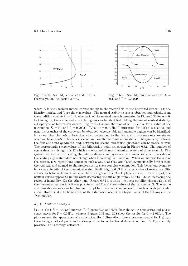
6.4. Mixed condition 116
0 0.5 1 1.5 2 2.50
5
10
15
20
25
Γ
Unstable
Stable
D
Figure 6.30: Stability curve D and Γ for athermosyphon inclination α = 0.
−150 −100 −50 0 50 100 150
−1
−0.8
−0.6
−0.4
−0.2
0
0.2
0.4
0.6
0.8
1
α [°]
Unstable
Unstable
Stable
Stable
Hopf Bifurcation
Hopf Bifurcation
w
Figure 6.31: Stability curve w vs. α for D =0.1, and Γ = 0.20029.
where A is the Jacobian matrix corresponding to the vector field of the linearized system, I is theidentity matrix, and λ are the eigenvalues. The neutral stability curve is obtained numerically fromthe condition that ℜ(λ) = 0. A schematic of the neutral curve is presented in Figure 6.30 for α = 0.In this figure, the stable and unstable regions can be identified. Along the line of neutral stability,a Hopf-type of bifurcation occurs. Figure 6.31 shows the plot of w − α curve for a value of theparameters D = 0.1 and Γ = 0.20029. When α = 0, a Hopf bifurcation for both the positive andnegative branches of the curve can be observed, where stable and unstable regions can be identified.It is clear that the natural branches which correspond to the first and third quadrants are stable,whereas the antinatural branches, second and fourth quadrants are unstable. The symmetry betweenthe first and third quadrants, and, between the second and fourth quadrants can be notice as well.The corresponding eigenvalues of the bifurcation point are shown in Figure 6.32. The number ofeigenvalues in this figure is 42 which are obtained from a dynamical system of dimension 42. Thissystem results from truncating the infinite dimensional system at a number for which the value ofthe leading eigenvalues does not change when increasing its dimension. When we increase the size ofthe system, new eigenvalues appear in such a way that they are placed symmetrically farther fromthe real axis and aligned to the previous set of slave complex eigenmodes. This behaviour seems tobe a characteristic of the dynamical system itself. Figure 6.33 illustrates a view of several stabilitycurves, each for a different value of the tilt angle α in a D − Γ plane at α = 0. In this plot, theneutral curves appear to unfold when decreasing the tilt angle from 75.5 to −32.5 increasing theregion of instability. On the other hand, Figure 6.34 illustrates the linear stability characteristics ofthe dynamical system in a w−α plot for a fixed Γ and three values of the parameter D. The stableand unstable regions can be observed. Hopf bifurcations occur for each branch of ecah particularcurve. However, it is to be notice that the bifurcation occurs at a higher value of the tilt angle whenD is smaller.
6.4.4 Nonlinear analysis
Let us select D = 1.5, and increase Γ. Figures 6.35 and 6.36 show the w − τ time series and phase-space curves for Γ = 0.95Γcr, whereas Figures 6.37 and 6.38 show the results for Γ = 1.01Γcr. Theplots suggest the appearance of a subcritical Hopf bifurcation. Two attractors coexist for Γ ≤ Γcr,these being a critical point and a strange attractor of fractional dimension. For Γ > Γcr, the onlypresence is of a strange attractor.
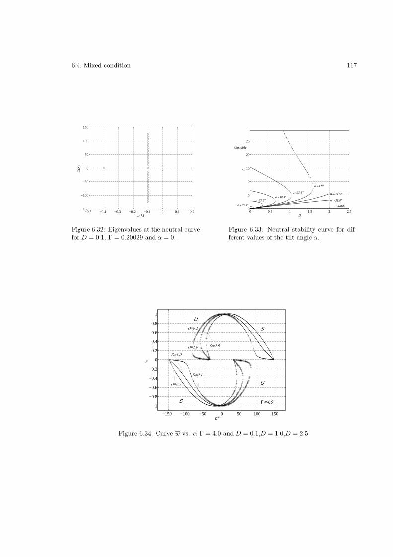
6.4. Mixed condition 117
−0.5 −0.4 −0.3 −0.2 −0.1 0 0.1 0.2−150
−100
−50
0
50
100
150
ℜ(λ)
ℑ(λ
)
Figure 6.32: Eigenvalues at the neutral curvefor D = 0.1, Γ = 0.20029 and α = 0.
0 0.5 1 1.5 2 2.50
5
10
15
20
25
Γ
D
Unstable
Stable
α=-32.5 °
α=-14.5 °
α=3.5 °
α=21.5 °α=39.5 °
α=57.5 °α=75.5 °
Figure 6.33: Neutral stability curve for dif-ferent values of the tilt angle α.
−150 −100 −50 0 50 100 150
−1
−0.8
−0.6
−0.4
−0.2
0
0.2
0.4
0.6
0.8
1
α°
w
D=0.1
D=2.5
D=2.5
D=0.1
D=1.0
D=1.0
S
U
S
U
Γ=4.0
Figure 6.34: Curve w vs. α Γ = 4.0 and D = 0.1,D = 1.0,D = 2.5.
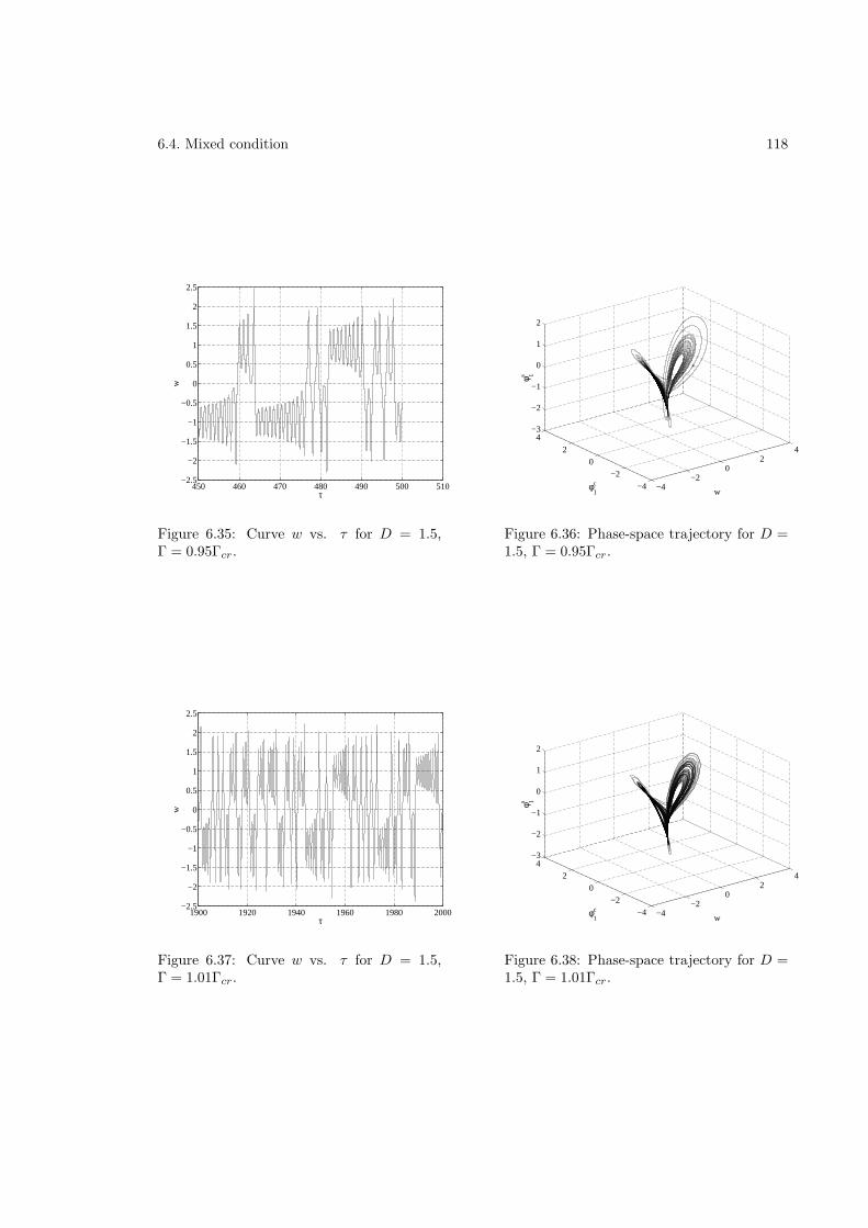
6.4. Mixed condition 118
450 460 470 480 490 500 510−2.5
−2
−1.5
−1
−0.5
0
0.5
1
1.5
2
2.5
τ
w
Figure 6.35: Curve w vs. τ for D = 1.5,Γ = 0.95Γcr.
−4−2
02
4
−4
−20
24
−3
−2
−1
0
1
2
wφ1c
φ 1s
Figure 6.36: Phase-space trajectory for D =1.5, Γ = 0.95Γcr.
1900 1920 1940 1960 1980 2000−2.5
−2
−1.5
−1
−0.5
0
0.5
1
1.5
2
2.5
τ
w
Figure 6.37: Curve w vs. τ for D = 1.5,Γ = 1.01Γcr.
−4−2
02
4
−4
−20
24
−3
−2
−1
0
1
2
wφ1c
φ 1s
Figure 6.38: Phase-space trajectory for D =1.5, Γ = 1.01Γcr.
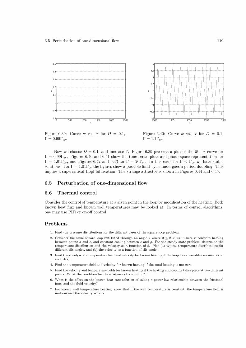
6.5. Perturbation of one-dimensional flow 119
0 500 1000 1500 2000 25000.8
0.9
1
1.1
1.2
1.3
1.4
1.5
τ
w
Figure 6.39: Curve w vs. τ for D = 0.1,Γ = 0.99Γcr.
1980 1985 1990 1995 2000−2
−1.5
−1
−0.5
0
0.5
1
1.5
2
τ
w
Figure 6.40: Curve w vs. τ for D = 0.1,Γ = 1.1Γcr.
Now we choose D = 0.1, and increase Γ. Figure 6.39 presents a plot of the w − τ curve forΓ = 0.99Γcr. Figures 6.40 and 6.41 show the time series plots and phase space representation forΓ = 1.01Γcr, and Figures 6.42 and 6.43 for Γ = 20Γcr. In this case, for Γ < Γcr we have stablesolutions. For Γ = 1.01Γcr the figures show a possible limit cycle undergoes a period doubling. Thisimplies a supercritical Hopf bifurcation. The strange attractor is shown in Figures 6.44 and 6.45.
6.5 Perturbation of one-dimensional flow
6.6 Thermal control
Consider the control of temperature at a given point in the loop by modification of the heating. Bothknown heat flux and known wall temperatures may be looked at. In terms of control algorithms,one may use PID or on-off control.
Problems
1. Find the pressure distributions for the different cases of the square loop problem.
2. Consider the same square loop but tilted through an angle θ where 0 ≤ θ < 2π. There is constant heatingbetween points a and c, and constant cooling between e and g. For the steady-state problem, determine thetemperature distribution and the velocity as a function of θ. Plot (a) typical temperature distributions fordifferent tilt angles, and (b) the velocity as a function of tilt angle.
3. Find the steady-state temperature field and velocity for known heating if the loop has a variable cross-sectionalarea A(s).
4. Find the temperature field and velocity for known heating if the total heating is not zero.
5. Find the velocity and temperature fields for known heating if the heating and cooling takes place at two differentpoints. What the condition for the existence of a solution?
6. What is the effect on the known heat rate solution of taking a power-law relationship between the frictionalforce and the fluid velocity?
7. For known wall temperature heating, show that if the wall temperature is constant, the temperature field isuniform and the velocity is zero.
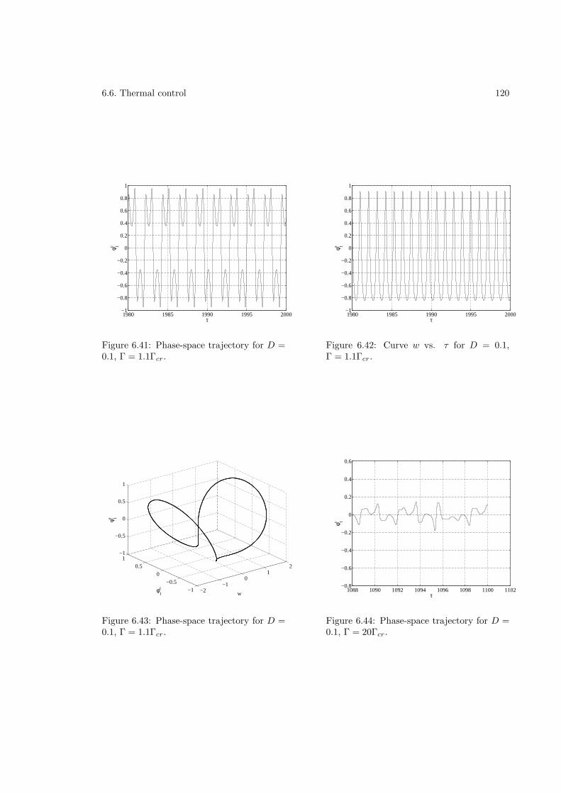
6.6. Thermal control 120
1980 1985 1990 1995 2000−1
−0.8
−0.6
−0.4
−0.2
0
0.2
0.4
0.6
0.8
1
τ
φ 1c
Figure 6.41: Phase-space trajectory for D =0.1, Γ = 1.1Γcr.
1980 1985 1990 1995 2000−1
−0.8
−0.6
−0.4
−0.2
0
0.2
0.4
0.6
0.8
1
τ
φ 1s
Figure 6.42: Curve w vs. τ for D = 0.1,Γ = 1.1Γcr.
−2−1
01
2
−1
−0.50
0.51
−1
−0.5
0
0.5
1
wφ1c
φ 1s
Figure 6.43: Phase-space trajectory for D =0.1, Γ = 1.1Γcr.
1088 1090 1092 1094 1096 1098 1100 1102−0.8
−0.6
−0.4
−0.2
0
0.2
0.4
0.6
τ
φ 1c
Figure 6.44: Phase-space trajectory for D =0.1, Γ = 20Γcr.
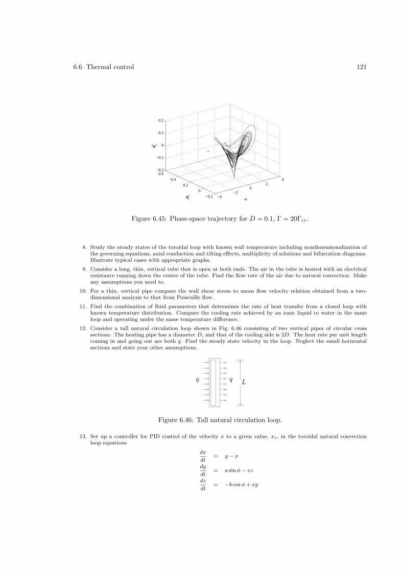
6.6. Thermal control 121
−4−2
02
4
−0.2
00.2
0.40.6
−0.2
−0.1
0
0.1
0.2
wφ1c
φ 1s
Figure 6.45: Phase-space trajectory for D = 0.1, Γ = 20Γcr.
8. Study the steady states of the toroidal loop with known wall temperature including nondimensionalization ofthe governing equations, axial conduction and tilting effects, multiplicity of solutions and bifurcation diagrams.Illustrate typical cases with appropriate graphs.
9. Consider a long, thin, vertical tube that is open at both ends. The air in the tube is heated with an electricalresistance running down the center of the tube. Find the flow rate of the air due to natural convection. Makeany assumptions you need to.
10. For a thin, vertical pipe compare the wall shear stress to mean flow velocity relation obtained from a two-dimensional analysis to that from Poiseuille flow.
11. Find the combination of fluid parameters that determines the rate of heat transfer from a closed loop withknown temperature distribution. Compare the cooling rate achieved by an ionic liquid to water in the sameloop and operating under the same temperature difference.
12. Consider a tall natural circulation loop shown in Fig. 6.46 consisting of two vertical pipes of circular crosssections. The heating pipe has a diameter D, and that of the cooling side is 2D. The heat rate per unit lengthcoming in and going out are both q. Find the steady state velocity in the loop. Neglect the small horizontalsections and state your other assumptions.
Lq q
Figure 6.46: Tall natural circulation loop.
13. Set up a controller for PID control of the velocity x to a given value, xs, in the toroidal natural convectionloop equations
dx
dt= y − x
dy
dt= a sin φ − xz
dz
dt= −b cos φ + xy
6.6. Thermal control 122
where a and b are held constant. Use the tilt angle φ as control input, and show numerical results.
Chapter 7
Moving boundary
7.1 Stefan problems
[44]The two phases, indicated by subscripts 1 and 2, are separated by an interface at x = X(t). In
each phase, the conduction equations is
∂2T1
∂x2− 1
κ1
∂T1
∂t= 0 (7.1)
∂2T2
∂x2− 1
κ2
∂T2
∂t= 0 (7.2)
At the interface the temperature should be continuous, so that
T1(X, t) = T2(X, t) (7.3)
Furthermore the difference in heat rate into the interface provides the energy required for phasechange. Thus
k1∂T1
∂x− k2
∂T2
∂x= Lρ
dX
dt(7.4)
7.1.1 Neumann’s solution
The material is initially liquid at T = T0. The temperature at the x = 0 end is reduced to zero fort > 0. Thus
T1 = 0 at x = 0 (7.5)
T2 → T0 as x→ ∞ (7.6)
Assume T1(x, t) to be
T1 = A erfx
2√κ1t
(7.7)
so that it satisfies equations (7.1) and (7.5). Similarly
T1 = A erfx
2√κ1t
T2 = T0 −B erfx
2√κ2t
(7.8)
123
7.1. Stefan problems 124
satisfies equation (7.2) and (7.6). The, condition (7.3) requires that
A erfx
2√κ1t
= T0 −B erfx
2√κ2t
= T1 (7.9)
This shows thatX = 2λ
√κ1t (7.10)
where λ is a constant. Using the remaining condition (7.4), we get
k1Ae−λ2 − k2B
√κ1
κ2e−κ1λ2/κ2 = λLκ1ρ
√π (7.11)
This can be written ase−λ2
erf λ− k2
√κ2
1(T0 − T1)e−κ2λ2/κ2
k1√κ2T1 erfc(λ
√κ1/κ2)
=λL
√π
c1T1s(7.12)
The temperatures are
T1 =T1
erf λerf (
x
2√κ1t
) (7.13)
T2 = T0 −T0 − T1
erfc(λ√κ1/κ2)
erfc(x
2√κ2t
) (7.14)
7.1.2 Goodman’s integral

Part IV
Multiple spatial dimensions
125
Chapter 8
Conduction
8.1 Steady-state problems
See [206].
8.2 Transient problems
8.2.1 Two-dimensional fin
The governing equation is
cρdx dyL∂T
∂t= Lk
(∂2T
∂x2+∂2T
∂y2
)− hdx dy(T − T∞) (8.1)
which simplifies to1
α
∂T
∂t=∂2T
∂x2+∂2T
∂y2−m2(T − T∞) (8.2)
where m2 = h/kL, the Biot number.In the steady state
∂2T
∂x2+∂2T
∂y2−m2(T − T∞) (8.3)
Consider a square of unit side with θ = T − T∞ being zero all around, except for one edgewhere it is unity.
Letθ(x, y) = X(x)Y (y) (8.4)
so that1
X
d2X
dx2= − 1
X
d2Y
dy2+m2 = −λ2 (8.5)
This leads to one equationd2X
dx2+ λ2X = 0 (8.6)
with X(0) = X(1) = 1. ThusX(x) = A sinλx+B cosλx (8.7)
126
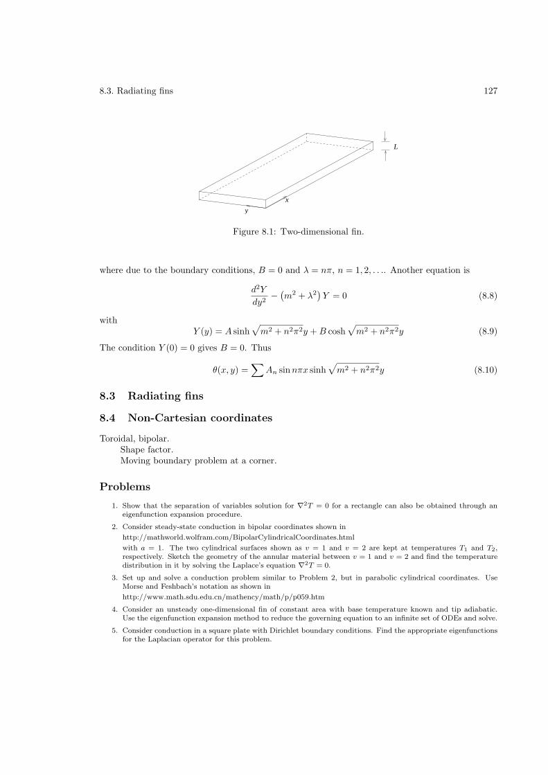
8.3. Radiating fins 127
x
y
L
Figure 8.1: Two-dimensional fin.
where due to the boundary conditions, B = 0 and λ = nπ, n = 1, 2, . . .. Another equation is
d2Y
dy2−(m2 + λ2
)Y = 0 (8.8)
withY (y) = A sinh
√m2 + n2π2y +B cosh
√m2 + n2π2y (8.9)
The condition Y (0) = 0 gives B = 0. Thus
θ(x, y) =∑
An sinnπx sinh√m2 + n2π2y (8.10)
8.3 Radiating fins
8.4 Non-Cartesian coordinates
Toroidal, bipolar.Shape factor.Moving boundary problem at a corner.
Problems
1. Show that the separation of variables solution for ∇2T = 0 for a rectangle can also be obtained through aneigenfunction expansion procedure.
2. Consider steady-state conduction in bipolar coordinates shown in
http://mathworld.wolfram.com/BipolarCylindricalCoordinates.html
with a = 1. The two cylindrical surfaces shown as v = 1 and v = 2 are kept at temperatures T1 and T2,respectively. Sketch the geometry of the annular material between v = 1 and v = 2 and find the temperaturedistribution in it by solving the Laplace’s equation ∇2T = 0.
3. Set up and solve a conduction problem similar to Problem 2, but in parabolic cylindrical coordinates. UseMorse and Feshbach’s notation as shown in
http://www.math.sdu.edu.cn/mathency/math/p/p059.htm
4. Consider an unsteady one-dimensional fin of constant area with base temperature known and tip adiabatic.Use the eigenfunction expansion method to reduce the governing equation to an infinite set of ODEs and solve.
5. Consider conduction in a square plate with Dirichlet boundary conditions. Find the appropriate eigenfunctionsfor the Laplacian operator for this problem.
Chapter 9
Forced convection
See [206].
9.1 Low Reynolds numbers
9.2 Potential flow
[169]If the heat flux is written as
q = ρcuT − k∇T (9.1)
the energy equation is∇ · q = 0 (9.2)
Heat flows along heatlines given by
dx
ρcTux − k(∂T/∂x)=
dy
ρcTuy − k(∂T/∂y)=
dz
ρcTuz − k(∂T/∂z)(9.3)
The tangent to heatlines at every point is the direction of the heat flux vector.
9.2.1 Two-dimensional flow
9.3 Leveque’s solution
Leveque (1928)
9.4 Multiple solutions
See [166].
9.5 Plate heat exchangers
There is flow on the two sides of a plate, 1 and 2, with an overall heat transfer coefficient of U .Consider a rectangular plate of size Lx×Ly in the x- and y-directions, respectively, as shown in Fig.
128
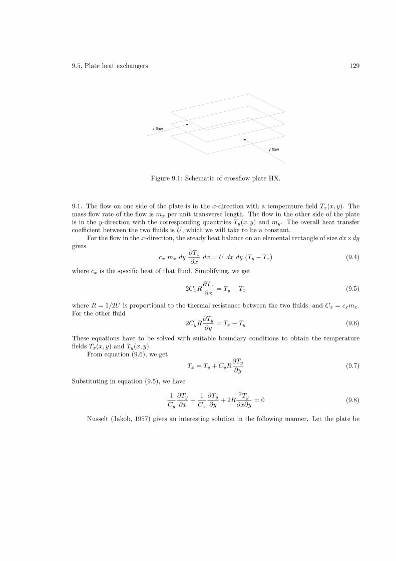
9.5. Plate heat exchangers 129
x flow
y flow
Figure 9.1: Schematic of crossflow plate HX.
9.1. The flow on one side of the plate is in the x-direction with a temperature field Tx(x, y). Themass flow rate of the flow is mx per unit transverse length. The flow in the other side of the plateis in the y-direction with the corresponding quantities Ty(x, y) and my. The overall heat transfercoefficient between the two fluids is U , which we will take to be a constant.
For the flow in the x-direction, the steady heat balance on an elemental rectangle of size dx×dygives
cx mx dy∂Tx
∂xdx = U dx dy (Ty − Tx) (9.4)
where cx is the specific heat of that fluid. Simplifying, we get
2CxR∂Tx
∂x= Ty − Tx (9.5)
where R = 1/2U is proportional to the thermal resistance between the two fluids, and Cx = cxmx.For the other fluid
2CyR∂Ty
∂y= Tx − Ty (9.6)
These equations have to be solved with suitable boundary conditions to obtain the temperaturefields Tx(x, y) and Ty(x, y).
From equation (9.6), we get
Tx = Ty + CyR∂Ty
∂y(9.7)
Substituting in equation (9.5), we have
1
Cy
∂Ty
∂x+
1
Cx
∂Ty
∂y+ 2R
2Ty
∂x∂y= 0 (9.8)
Nusselt (Jakob, 1957) gives an interesting solution in the following manner. Let the plate be
9.5. Plate heat exchangers 130
of dimensions L and W in the x- and y-directions. Nondimensional variables are
ξ =x
L(9.9)
η =y
W(9.10)
θx =Tx − Ty,i
Tx,i − Ty,i(9.11)
θy =Ty − Ty,i
Tx,i − Ty,i(9.12)
a =UWL
Cx(9.13)
b =UWL
Cy(9.14)
The governing equations are then
a(θx − θy) = −∂θx
∂ξ(9.15)
b(θx − θy) =∂θy
∂η(9.16)
with boundary conditions
θx = 1 at ξ = 0 (9.17)
θy = 0 at η = 0 (9.18)
Equation (9.16) can be written as
∂θy
∂η+ bθy = bθx (9.19)
Solving for θy we get
θy = e−bη
(C(ξ) + b
∫ η
0
θx(ξ, η′)ebη′
dη′)
(9.20)
From the boundary condition (9.18), we get
C = 0 (9.21)
so that
θy(ξ, η) = be−bη
∫ η
0
θx(ξ, η′)ebη′
dη′ (9.22)
Using the same procedure, from equation (9.15) we get
θx(ξ, η) = e−aξ + ae−aξ
∫ ξ
0
θy(ξ′, η)eaξ′
dξ′ (9.23)
Substituting for θy, we find the Volterra integral equation
θx(ξ, η) = e−aξ + abe−(aξ+bη)
∫ ξ
0
∫ η
0
θx(ξ′, η′)eaξ′+bη′
dξ′ dη′ (9.24)
9.5. Plate heat exchangers 131
for the unknown θx.We will first solve the Volterra equation for an arbitrary λ, where
θx(ξ, η) = e−aξ + abλe−(aξ+bη)
∫ ξ
0
∫ η
0
θx(ξ′, η′)eaξ′+bη′
dξ′ dη′ (9.25)
Let us express the solution in terms of a finite power series
θx(ξ, η) = φ0(ξ, η) + λφ1(ξ, η) + λ2φ2(ξ, η) + . . .+ λnφn(ξ, η) (9.26)
This can be substituted in the integral equation. Since λ is arbitrary, the coefficient of each orderof λ must vanish. Thus
φ0(ξ, η) = e−aξ (9.27)
φ1(ξ, η) = abe−(aξ+bη)
∫ ξ
0
∫ η
0
φ0(ξ′, η′)eaξ′+bη′
dξ′ dη′ (9.28)
φ2(ξ, η) = abe−(aξ+bη)
∫ ξ
0
∫ η
0
φ1(ξ′, η′)eaξ′+bη′
dξ′ dη′ (9.29)
... (9.30)
φn(ξ, η) = abe−(aξ+bη)
∫ ξ
0
∫ η
0
φn−1(ξ′, η′)eaξ′+bη′
dξ′ dη′ (9.31)
(9.32)
The solutions are
φ0 = e−aξ (9.33)
φ1 = aξe−aξ(1 − e−bη) (9.34)
φ2 =1
2a2ξ2e−aξ(1 − e−bη − bηe−bη) (9.35)
φ3 =1
2 × 3a3ξ3e−aξ(1 − e−bη − bηe−bη − 1
2b2η2e−bη) (9.36)
... (9.37)
φn =1
n!anξne−aξ(1 − e−bη − bηe−bη − . . .− 1
(n− 1)!bn−1ηn−1e−bη) (9.38)
Substituting into the expansion, equation (9.26), and taking λ = 1, we get
θx(ξ, η) = φ0(ξ, η) + φ1(ξ, η) + φ2(ξ, η) + . . .+ φn(ξ, η) (9.39)
where the φs are given above.
Example 9.1Find a solution of the same problem by separation of variables.Taking
Ty(x, y) = X(x)Y (y) (9.40)
Substituting and dividing by XY , we get
1
Cx
∂Tx
∂x+
1
Cy
dY
dy+ 2R = 0 (9.41)
9.6. Falkner-Skan boundary flows 132
Since the first term is a function only of x, and the second only of y, each must be a constant. Thus we canwrite
dX
dx+
1
cxmx(a + R)X = 0 (9.42)
dY
dy+
1
cymy(a − R)Y = 0 (9.43)
where a is a constant. Solving the two equations and taking their product, we have
Ty =c
a + Rexp
»
− x
cxmx(a + R)+
y
cymy(a − R)
–
(9.44)
where c is a constant. Substituting in equation (9.7), we get
Tx =c
a − Rexp
»
− x
cxmx(a + R)+
y
cymy(a − R)
–
(9.45)
The rate of heat transfer over the entire plate, Q, is given by
Q = Cx
Z L−y
0[Tx(Lx, y) − Tx(0, y)] dy (9.46)
= cCxCy exp
»
− lx
Cx(a + R)− Ly
C2(a − R)− 2
–
(9.47)
The heat rate can be maximized by varying either of the variables Cx or Cy .
9.6 Falkner-Skan boundary flows
Problems
1. This is a problem
Chapter 10
Natural convection
10.1 Governing equations
10.2 Cavities
10.3 Marangoni convection
See [204].
Problems
1. This is a problem.
133
Chapter 11
Porous media
[103,130,201]
11.1 Governing equations
The continuity equation for incompressible flow in a porous medium is
∇ · V = 0 (11.1)
11.1.1 Darcy’s equation
For the momentum equation, the simplest model is that due to Darcy
∇p = − µ
KV + ρf (11.2)
where f is the body force per unit mass. Here K is called the permeability of the medium andhas units of inverse area. It is similar to the incompressible Navier-Stokes equation with constantproperties where the inertia terms are dropped and the viscous force per unit volume is representedby −(µ/K)V. Sometimes a term cρ0∂V/∂t is added to the left side for transient problems, but itis normally left out because it is very small. The condition on the velocity is that of zero normalvelocity at a boundary, allowing for slip in the tangential direction.
From equations (11.1) and (11.2), for f = 0 we get
∇2p = 0 (11.3)
from which the pressure distribution can be determined.
11.1.2 Forchheimer’s equation
Forchheimer’s equation which is often used instead of Darcy’s equation is
∇p = − µ
KV − cfK
−1/2ρ|V|V + ρf (11.4)
where cf is a dimensionless constant. There is still slip at a boundary.
134
11.2. Forced convection 135
11.1.3 Brinkman’s equation
Another alternative is Brinkman’s equation
∇p = − µ
KV + µ∇2V + ρf (11.5)
where µ is another viscous coefficient. In this model there is no slip at a solid boundary.
11.1.4 Energy equation
The energy equation is
(ρc)m∂T
∂t+ ρcpV · ∇T = km∇2T (11.6)
where km is the effective thermal conductivity, and
(ρc)m = φρcp + (1 − φ)(ρc)m (11.7)
is the average heat capacity. The subscripts m refers to the solid matrix, and φ is the porosity ofthe material. An equivalent form is
σ∂T
∂t+ V · ∇T = αm∇2T (11.8)
where
αm =km
ρcp(11.9)
σ =(ρc)m
ρcp(11.10)
See [1].
11.2 Forced convection
11.2.1 Plane wall at constant temperature
The solution to
∂u
∂x+∂v
∂y= 0 (11.11)
u = −Kµ
∂p
∂x(11.12)
v = −Kµ
∂p
∂y(11.13)
is
u = U (11.14)
v = 0 (11.15)
ForUx
αm= Pex ≫ 1 (11.16)
11.2. Forced convection 136
the energy equation is
u∂T
∂x+ v
∂T
∂y= αm
∂2T
∂y2(11.17)
or
U∂T
∂x= αm
∂2T
∂y2(11.18)
The boundary conditions are
T (0) = Tw (11.19)
T (∞) = T∞ (11.20)
Writing
η = y
√U
αmx(11.21)
θ(η) =T − Tw
T∞ − Tw(11.22)
we get
∂T
∂x= (T∞ − Tw)
dθ
dη
∂η
∂x(11.23)
= (T∞ − Tw)dθ
dη
(−y√
U
αm
1
2x−3/2
)(11.24)
∂T
∂y= (T∞ − Tw)
dθ
dη
∂η
∂y(11.25)
= (T∞ − Tw)dθ
dη
√U
αmx(11.26)
∂2T
∂y2= (T∞ − Tw)
d2θ
dη2
U
αmx(11.27)
so that the equation becomes
θ′′ +1
2η θ′ = 0 (11.28)
with
θ(0) = 0 (11.29)
θ(∞) = 1 (11.30)
We multiply by the integrating factor eη2/4 to get
d
dη
(eη2/4θ′
)= 0 (11.31)
The first integral is
θ′ = C1e−η2/4 (11.32)
Integrating again we have
θ = C1
∫ η
0
e−η′2/4 dη′ + C2 (11.33)
11.2. Forced convection 137
With the change in variables x = η′/2, the solution becomes
θ = 2C1
∫ η/2
0
e−x2
dx (11.34)
Applying the boundary conditions, we find that C1 = 1/√π and C2 = 0. Thus
θ =2√π
∫ η/2
0
e−x2
dx (11.35)
= erfη
2(11.36)
The heat transfer coefficient is defined as
h =q′′
Tw − T∞(11.37)
= − km
Tw − T∞
∂T
∂y(11.38)
= km∂θ
∂y(11.39)
The local Nusselt number is given by
Nux =hx
km(11.40)
= x∂θ
∂y
∣∣∣∣∣y=0
(11.41)
=1√π
√Ux
αm(11.42)
=1√πPe−1/2
x (11.43)
Example 11.1Find the temperature distribution for flow in a porous medium parallel to a flat plate with uniform heat
flux.
11.2.2 Stagnation-point flow
For flow in a porous medium normal to an infinite flat plate, the velocity field is
u = Cx (11.44)
v = −Cy (11.45)
The energy equation is
Cx∂T
∂x− Cy
∂T
∂y= αm
∂2T
∂y2(11.46)
11.2. Forced convection 138
11.2.3 Thermal wakes
Line source
For Pex ≫ 1, the governing equation is
U∂T
∂x= αm
∂2T
∂y2(11.47)
where the boundary conditions are
∂T
∂y= 0 at y = 0 (11.48)
q′ = (ρcp)U
∫∞
−∞
(T − T∞) dy (11.49)
Writing
η = y
√U
αmx(11.50)
θ(η) =T − T∞q′/km
√Ux
αm(11.51)
we find that
∂T
∂x= θ
q′
km
√αm
U
(−1
2x−3/2
)+dθ
dηy
√U
αm
(−1
2x−3/2 q
′
km
√αm
Ux
)(11.52)
∂T
∂y=
q′
km
√αm
Ux
dθ
dη
√U
αmx(11.53)
∂2T
∂y2=
q′
km
√αm
Ux
dθ
dη
U
αmx(11.54)
(11.55)
Substituting in the equation, we get
θ′′ = −1
2(θ + ηθ′) (11.56)
The conditions (11.48)-(11.49) become
∂θ
∂η= 0 at η = 0 (11.57)
∫∞
−∞
θ dy = 1 (11.58)
The equation (11.56) can be written as
θ′′ = −1
2
d
dη(ηθ) (11.59)
which integrates to
θ′ = −1
2ηθ + C1 (11.60)
11.3. Natural convection 139
Since θ′ = 0 at η = 0, we find that C1 = 0. Integrating again, we get
θ = C2e−η2/4 (11.61)
Substituting in the other boundary condition
1 =
∫∞
−∞
θ dη = C2
∫∞
−∞
e−η2/4 dη = 2√πC2 (11.62)
from which
C2 =1
2√π
(11.63)
Thus the solution is
θ =1
2√πe−η2/4 (11.64)
or
T − T∞ =1
2√π
q′
km
√(αm
Ux) exp(
−Uy2
4αmx) (11.65)
Example 11.2Show that for a point source
T − T∞ =q
4πkxexp(
−Ur2
4αmx) (11.66)
11.3 Natural convection
11.3.1 Linear stability
This is often called the Horton-Rogers-Lapwood problem, and consists of finding the stability of ahorizontal layer of fluid in a porous medium heated from below. The geometry is shown in Fig. 11.1.
A
B
gravity
x
y
Figure 11.1: Stability of horizontal porous layer.
The governing equations are
∇ · V = 0 (11.67)
−∇p− µ
KV + ρg = 0 (11.68)
σ∂T
∂t+ V · ∇T = αm∇2T (11.69)
ρ = ρ0 [1 − β (T − T0)] (11.70)
11.3. Natural convection 140
where g = −gj. The basic steady solution is
V = 0 (11.71)
T = T0 + ∆T(1 − y
H
)(11.72)
p = p0 − ρ0g
[y +
1
2β∆T
(y2
H− 2y
)](11.73)
For constant heat flux ∆T = q′′s /km. We apply a perturbation to each variable as
V = V + V′ (11.74)
T = T + T ′ (11.75)
p = p+ p′ (11.76)
Substituting and linearizing
∇ · V′ = 0 (11.77)
−∇p′ − µ
KV′ − βρ0T
′g = 0 (11.78)
∂T ′
∂t− ∆T
Hw′ = αm∇2T ′ (11.79)
Using the nondimensional variables
x∗ =x
H(11.80)
t∗ =αmt
σH2(11.81)
V∗ =HV′
αm(11.82)
T ∗ =T ′
∆T(11.83)
p∗ =Kp′
µαm(11.84)
the equations become, on dropping *s
∇ · V = 0 (11.85)
−∇p− V +Ra Tk = 0 (11.86)
∂T
∂t− w = ∇2T (11.87)
where
Ra =ρ0gβKH∆T
µαm(11.88)
From these equations we get∇2w = Ra∇2
HT (11.89)
where
∇H =∂2
∂x2(11.90)
11.3. Natural convection 141
Using separation of variables
w(x, y, z, t) = W (y) exp (st+ ikxx) (11.91)
T (x, y, z, t) = Θ(y) exp (st+ ikxx) (11.92)
Substituting into the equations we get
(d2
dy2− k2 − s
)Θ = −W (11.93)
(d2
dy2− k2
)W = −k2Ra Θ (11.94)
wherek2 = k2
x + k2y (11.95)
Isothermal boundary conditions
The boundary conditions are W = Θ = 0 at either wall. For the solutions to remain bounded asx, y → ∞, the wavenumbers kx and ky must be real. Furthermore, since the eigenvalue problem isself-adjoint, as shown below, it can be shown that s is also real.
For a self-adjoint operator L, we must have
(u,Lv) = (Lu, v) (11.96)
If
vL(u) − uL(v) =∂P
∂x+∂Q
∂y(11.97)
then∫
V
[vL(u) − uL(v)] dV =
∫ (∂P
∂x+∂Q
∂y
)dV (11.98)
=
∫
V
∇ · (P i +Qj) dV (11.99)
=
∫
S
n · (P i +Qj) (11.100)
If n·(P i+Qj) = 0 at the boundaries (i.e. impermeable), which is the case here, then L is self-adjoint.Thus, marginal stability occurs when s = 0, for which
(d2
dy2− k2
)Θ = −W (11.101)
(d2
dy2− k2
)W = −k2Ra Θ (11.102)
from which (d2
dy2− k2
)2
W = k2Ra W (11.103)
The eigenfunctions areW = sinnπy (11.104)
11.3. Natural convection 142
where n = 1, 2, 3, . . ., as long as
Ra =
(n2π2
k+ k
)2
(11.105)
For each n there is a minimum value of the critical Rayleigh number determined by
dRa
dk= 2
(n2π2
k+ k
)[−n
2π2
k2+ 1
](11.106)
The lowest critical Ra is with k = π and n = 1, which gives
Rac = 4π2 (11.107)
for the onset of instability.
Constant heat flux conditions
Here W = dΘ/dy = 0 at the walls. We write
W = W0 + α2W1 + . . . (11.108)
Θ = Θ0 + α2Θ1 + . . . (11.109)
Ra = Ra0 + α2Ra1 + . . . (11.110)
For the zeroth order systemd2W0
dy2= 0 (11.111)
with W0 = dΘ0/dy = 0 at the walls. The solutions is W0 = 0, Θ0 = 1. To the next order
d2W1
dy2= W0 −Ra0Θ0 (11.112)
d2Θ1
dy2+W1 = Θ0 (11.113)
with W1 = dΘ1/dy = 0 at the walls. Finally, we get Rac = 12.
11.3.2 Steady-state inclined layer solutions
Consider an inclined porous layer of thickness H at angle φ with respect to the horizontal shown inFig. 11.2
Introducing the streamfunction ψ(x, y), where
u =∂ψ
∂y(11.114)
v = −∂ψ∂x
(11.115)
Darcy’s equation becomes
−∂p∂x
− µ
K
∂ψ
∂y= ρ0g [1 − β(T − T0)] sinφ (11.116)
−∂p∂y
+µ
K
∂ψ
∂x= ρ0g [1 − β(T − T0)] cosφ (11.117)
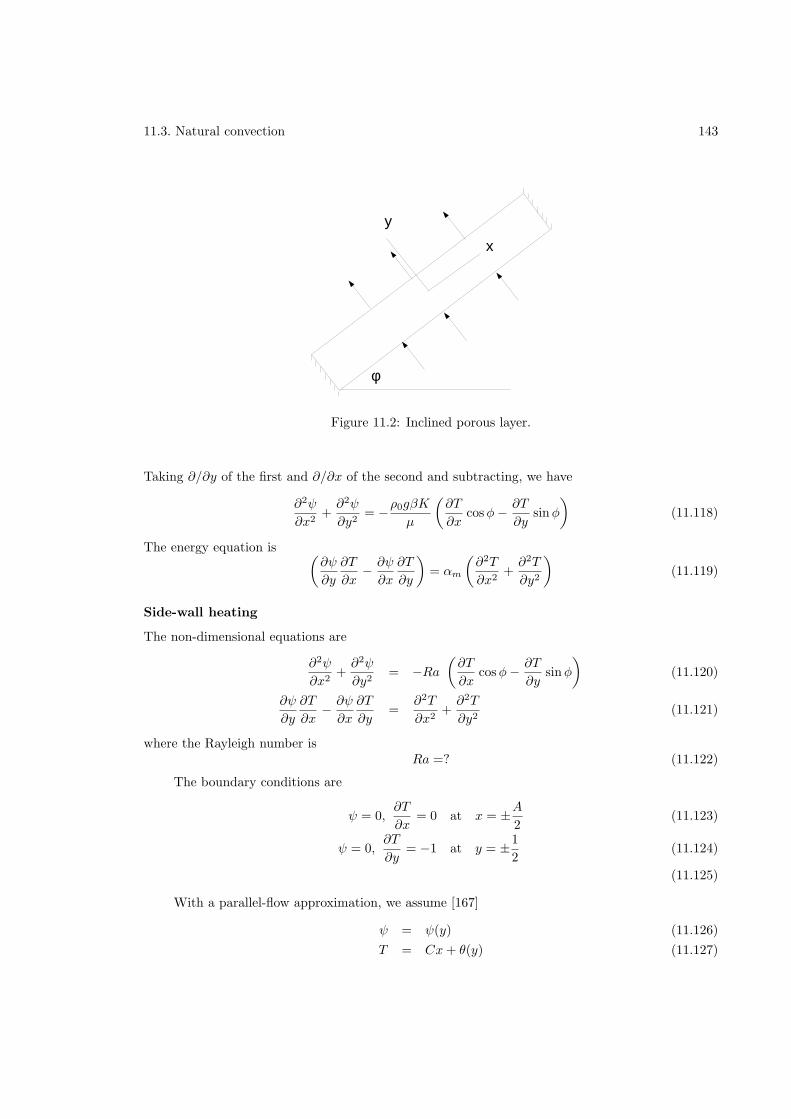
11.3. Natural convection 143
x
y
φ
Figure 11.2: Inclined porous layer.
Taking ∂/∂y of the first and ∂/∂x of the second and subtracting, we have
∂2ψ
∂x2+∂2ψ
∂y2= −ρ0gβK
µ
(∂T
∂xcosφ− ∂T
∂ysinφ
)(11.118)
The energy equation is (∂ψ
∂y
∂T
∂x− ∂ψ
∂x
∂T
∂y
)= αm
(∂2T
∂x2+∂2T
∂y2
)(11.119)
Side-wall heating
The non-dimensional equations are
∂2ψ
∂x2+∂2ψ
∂y2= −Ra
(∂T
∂xcosφ− ∂T
∂ysinφ
)(11.120)
∂ψ
∂y
∂T
∂x− ∂ψ
∂x
∂T
∂y=
∂2T
∂x2+∂2T
∂y2(11.121)
where the Rayleigh number isRa =? (11.122)
The boundary conditions are
ψ = 0,∂T
∂x= 0 at x = ±A
2(11.123)
ψ = 0,∂T
∂y= −1 at y = ±1
2(11.124)
(11.125)
With a parallel-flow approximation, we assume [167]
ψ = ψ(y) (11.126)
T = Cx+ θ(y) (11.127)
11.3. Natural convection 144
The governing equations become
∂2ψ
∂y2−Ra sinφ
dθ
dy+RC cosφ = 0 (11.128)
d2θ
dy2− C
dψ
dy= 0 (11.129)
An additional constraint is the heat transported across a transversal section should be zero. Thus
∫ 1/2
−1/2
(uT − ∂T
∂x
)dy = 0 (11.130)
Let us look at three cases.(a) Horizontal layer
For φ = 0 the temperature and streamfunction are
T = Cx− y
[1 +
RaC2
24
(4y2 − 3
)](11.131)
ψ = −RaC8
(4y2 − 1
)(11.132)
Substituting in condition (11.130), we get
C(10R−Ra2C2 − 120
)= 0 (11.133)
the solutions of which are
C = 0 (11.134)
C =1
Ra
√10(Ra− 12) (11.135)
C = − 1
Ra
√10(Ra− 12) (11.136)
The only real solution that exists for Ra ≤ 12 is the conductive solution C = 0. For C > 12, thereare two nonzero values of C which lead to convective solutions, for which
ψc =RaC
8(11.137)
Nu =12
12 −RaC2(11.138)
For φ = 180, the only real value of C is zero, so that only the conductive solution exists.(b) Natural circulation
Let us take C sinφ > 0, for which we get
ψc =B
C
(1 − cosh
α
2
)(11.139)
Nu = − α
2B sinh α2 + αC cotφ
(11.140)
where
α2 = RC sinφ (11.141)
B = −1 + C cotφ
cosh α2
(11.142)
11.3. Natural convection 145
and the constant C is determined from
C − B2
2C
(sinhα
α− 1
)−B cotφ
(cosh
α
2− 2
αsinh
α
2
)= 0 (11.143)
(c) Antinatural circulationFor C sinφ < 0, for which we get
ψc =B
C
(1 − cosh
β
2
)(11.144)
Nu = − β
2B sinh β2 + βC cotφ
(11.145)
where
β2 = −RC sinφ (11.146)
B = −1 + C cotφ
cosh β2
(11.147)
and the constant C is determined from
C − B2
2C
(sinβ
β− 1
)−B cotφ
(cosh
β
2− 2
βsinh
β
2
)= 0 (11.148)
End-wall heating
Darcy’s law is
∇2ψ = R
(∂T
∂xsinφ+
∂T
∂ycosφ
)(11.149)
The boundary conditions are
ψ = 0,∂T
∂x= −1 at x = ±A
2(11.150)
ψ = 0,∂T
∂y= 0 at x = ±1
2(11.151)
With a parallel-flow approximation, we assume
ψ = ψ(y) (11.152)
T = Cx+ θ(y) (11.153)
The governing equations become
dθ
dy2− C
dψ
dy= 0 (11.154)
∂2ψ
∂y2−R cosφ
dθ
dy−RC sinφ = 0 (11.155)
An additional constraint is the heat transported across a transversal section. Thus
∫ 1/2
−1/2
(uT − ∂T
∂x
)dy = 1 (11.156)
11.3. Natural convection 146
Let us look at three cases.(a) Vertical layer
For φ = 0 the temperature and streamfunction are
T = Cx+B1
αsin(αy) − B2
αcos(αy) (11.157)
ψ =B1
Ccos(αy) +
B2
Csin(αy) +B3 (11.158)
whereα2 = −RC (11.159)
Substituting in condition (11.130), we get
C(10R−R2C2 − 120
)= 0 (11.160)
the solutions of which are
C = 0 (11.161)
C =1
R
√10(R− 12) (11.162)
C = − 1
R
√10(R− 12) (11.163)
The only real solution that exists for R ≤ 12 is the conductive solution C = 0. For C > 12, thereare two nonzero values of C which lead to convective solutions, for which
ψc =RC
8(11.164)
Nu =12
12 −RC(11.165)
For φ = 180, the only real value of C is zero, so that only the conductive solution exists.(b) Natural circulation
Let us take C sinφ > 0, for which we get
ψc =B
C
(1 − cosh
α
2
)(11.166)
Nu = − α
2B sinh α2 + αC cotφ
(11.167)
where
α2 = RC sinφ (11.168)
B = −1 + C cotφ
cosh α2
(11.169)
and the constant C is determined from
C − B2
2C
(sinhα
α− 1
)−B cotφ
(cosh
α
2− 2
αsinh
α
2
)= 0 (11.170)
(c) Antinatural circulation
11.3. Natural convection 147
For C sinφ > 0, for which we get
ψc =B
C
(1 − cosh
β
2
)(11.171)
Nu = − β
2B sinh β2 + βC cotφ
(11.172)
where
β2 = −RC sinφ (11.173)
B = −1 + C cotφ
cosh β2
(11.174)
and the constant C is determined from
C − B2
2C
(sinβ
β− 1
)−B cotφ
(cosh
β
2− 2
βsinh
β
2
)= 0 (11.175)
Problems
1. This is a problem.
Chapter 12
Moving boundary
12.1 Stefan problems
148
Part V
Complex systems
149
Chapter 13
Radiation
13.1 Monte Carlo methods
[209][219] is a review of the radiative properties of semiconductors.
Problems
1. Consider an unsteady n-body radiative problem. The temperature of the ith body is given by
MjcjdTj
dt= −
nX
i=1
AiFijσ(T 4i − T 4
j ) + Qj
= Aj
nX
i=1
Fjiσ(T 4i − T 4
j ) + Qj
What kind of dynamic solutions are possible?
2. The steady-state temperature distribution in a one-dimensional radiative fin is given by
dT
dx+ hT 4 = 0
Is the solution unique and always possible?
3. Show that between one small body 1 and its large surroundings 2, the dynamics of the small-body temperatureis governed by
M1c1dT1
dt= −A1F12σ(T 4
1 − T 42 ) + Q1.
150
Chapter 14
Boiling and condensation
14.1 Homogeneous nucleation
151
Chapter 15
Microscale heat transfer
[108] is a review of microscale heat exchangers, and [36] of photonic devices.[86,119,178,186,202,219]
15.1 Diffusion by random walk
15.1.1 One-dimensional
Consider a walker along an infinite straight line moving with a step size ∆x taken forward orbackward with equal probability in a time interval ∆t. Let the current position of the walker bex, and the probability that the walker is in an interval [x − dx/2, x + dx/2] be P (x, t). Sincethere is equal probability of the walker in the previous time step to have been in the interval[x− ∆x− dx/2, x− ∆x+ dx/2] or [x+ ∆x− dx/2, x+ ∆x+ dx/2], we have
P (x, t) =1
2[P (x− ∆x, t− ∆t) + P (x+ ∆x, t− ∆t] . (15.1)
Assuming that ∆x and ∆t are small, Taylor series expansions give
P (x± ∆x, t− ∆t) = P ± ∂P
∂x∆x− ∂P
∂t∆t
+1
2
∂2P
∂x2∆x2 ± ∂2P
∂x∂t∆x∆t+
1
2
∂2P
∂t2∆t2
±1
6
∂3P
∂x3∆x3 − 1
2
∂3P
∂x2∂t∆x2∆t± 1
2
∂3P
∂x∂t2∆x∆t2 − 1
6
∂3P
∂t3∆t3
+ . . . , (15.2)
where the terms on the right side are evaluated at (x, t). Substituting in Eq. (15.1) we get
∂P
∂t−D
∂2P
∂x2=
1
2
∂2P
∂t2∆t− 1
2
∂3P
∂x2∂t∆x2 + . . . , (15.3)
where D = ∆x2/2∆t. If we let ∆x → 0 and ∆t → 0 such that D is constant, we get the diffusionequation
∂P
∂t= D
∂2P
∂x2. (15.4)
152
15.2. Boltzmann transport equation 153
15.1.2 Multi-dimensional
Let P = P (r, t), and ∆r be a step in any direction where |∆r| is a constant. Then
P (r, t) =
∫
S
P (r + ∆r, t− ∆t) dS (15.5)
where S is a sphere of radius |∆r| centered on r. Also
P (r + ∆r, t− ∆t) = P +∂P
∂ri∆ri −
∂P
∂t∆t
1
2
∂2P
∂ri∂ri+ . . . (15.6)
etc.
15.2 Boltzmann transport equation
The classical distribution function f(r,v, t) is defined as number of particles in the volume dr dv inthe six-dimensional space of coordinates r and velocity v. Following a volume element in this space,we have the balance equation [109,123,124]
∂f
∂t+ v · ∇f + a · ∂f
∂v=
(∂f
∂t
)
scat
, (15.7)
where a = dv/dt is the acceleration due to an external force. The term on the right side is due tocollisions and scattering. The heat flux is then
q(r, t) =
∫v(r, t)f(r, ε, t)εD dε, (15.8)
where D(ε) is the density of energy states ε.
15.2.1 Relaxation-time approximation
Under this approximation (∂f
∂t
)
scat
=f0 − f
τ, (15.9)
where τ = τ(r,v). Thus∂f
∂t+ v · ∇f + a · ∂f
∂v=f0 − f
τ. (15.10)
Several further approximations can be made.
(a) Fourier’s lawAssume ∂/∂t = 0, a = 0 and ∇f = ∇f0 in the left side of Eq. (15.10) so that
f = f0 − τv · ∇f0. (15.11)
Introducing explicitly the dependence of f on temperature, we can write
∇f0 =df0dT
∇T. (15.12)
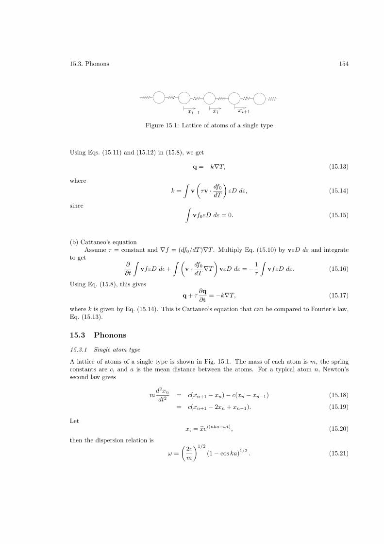
15.3. Phonons 154
xi−1 xi xi+1
Figure 15.1: Lattice of atoms of a single type
Using Eqs. (15.11) and (15.12) in (15.8), we get
q = −k∇T, (15.13)
where
k =
∫v
(τv · df0
dT
)εD dε, (15.14)
since ∫vf0εD dε = 0. (15.15)
(b) Cattaneo’s equationAssume τ = constant and ∇f = (df0/dT )∇T . Multiply Eq. (15.10) by vεD dε and integrate
to get∂
∂t
∫vfεD dǫ+
∫ (v · df0
dT∇T)
vεD dε = −1
τ
∫vfεD dε. (15.16)
Using Eq. (15.8), this gives
q + τ∂q
∂t= −k∇T, (15.17)
where k is given by Eq. (15.14). This is Cattaneo’s equation that can be compared to Fourier’s law,Eq. (15.13).
15.3 Phonons
15.3.1 Single atom type
A lattice of atoms of a single type is shown in Fig. 15.1. The mass of each atom is m, the springconstants are c, and a is the mean distance between the atoms. For a typical atom n, Newton’ssecond law gives
md2xn
dt2= c(xn+1 − xn) − c(xn − xn−1) (15.18)
= c(xn+1 − 2xn + xn−1). (15.19)
Letxi = xei(nka−ωt), (15.20)
then the dispersion relation is
ω =
(2c
m
)1/2
(1 − cos ka)1/2
. (15.21)
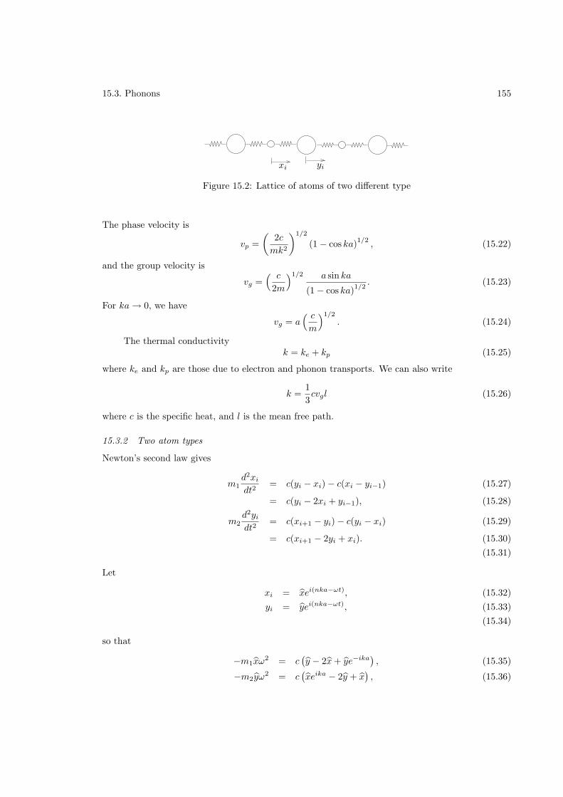
15.3. Phonons 155
xi yi
Figure 15.2: Lattice of atoms of two different type
The phase velocity is
vp =
(2c
mk2
)1/2
(1 − cos ka)1/2
, (15.22)
and the group velocity is
vg =( c
2m
)1/2 a sin ka
(1 − cos ka)1/2
. (15.23)
For ka→ 0, we have
vg = a( cm
)1/2
. (15.24)
The thermal conductivityk = ke + kp (15.25)
where ke and kp are those due to electron and phonon transports. We can also write
k =1
3cvgl (15.26)
where c is the specific heat, and l is the mean free path.
15.3.2 Two atom types
Newton’s second law gives
m1d2xi
dt2= c(yi − xi) − c(xi − yi−1) (15.27)
= c(yi − 2xi + yi−1), (15.28)
m2d2yi
dt2= c(xi+1 − yi) − c(yi − xi) (15.29)
= c(xi+1 − 2yi + xi). (15.30)
(15.31)
Let
xi = xei(nka−ωt), (15.32)
yi = yei(nka−ωt), (15.33)
(15.34)
so that
−m1xω2 = c
(y − 2x+ ye−ika
), (15.35)
−m2yω2 = c
(xeika − 2y + x
), (15.36)
15.4. Thin films 156
which can also be written as[
2c−m1ω2 −c(1 + e−ika)
−c(1 + eika) 2c−m2ω2
] [xy
]=
[00
]. (15.37)
This means that(2c−m1ω
2)(2c−m2ω2) − c2(1 + e−ika)(1 + eika) = 0, (15.38)
which simplifies tom1m2ω
4 − 2c(m1 +m2)ω2 + 2c2(1 − cos ka) = 0. (15.39)
The solution is
ω2 =1
2m1m2
[2c(m1 +m2) ± 2c
√m2
1 +m22 + 2m1m2 cos ka
]. (15.40)
The positive sign corresponds to the optical and the negative to the acoustic mode.
15.4 Thin films
Chapter 16
Bioheat transfer
16.1 Mathematical models
Good references are [35,53].
157
Chapter 17
Heat exchangers
17.1 Fin analysis
Analysis of Kraus (1990) for variable heat transfer coefficients.
17.2 Porous medium analogy
See Nield and Bejan, p. 87 [130].
17.3 Heat transfer augmentation
17.4 Maldistribution effects
Rohsenow (1981)
17.5 Microchannel heat exchangers
Phillips (1990).
17.6 Radiation effects
See Ozisik (1981).Shah (1981)
17.7 Transient behavior
Ontko and Harris (1990)For both fluids mixed
McdT
dt+ m1c1(T
in1 − T out
1 ) + mc2(Tin2 − T out
2 ) = 0 (17.1)
For one fluid mixed and the other unmixed, we have
ρAc2∂T2
∂t+ ρV2Ac2
∂T2
∂x+ hP (T − T1) = 0 (17.2)
158
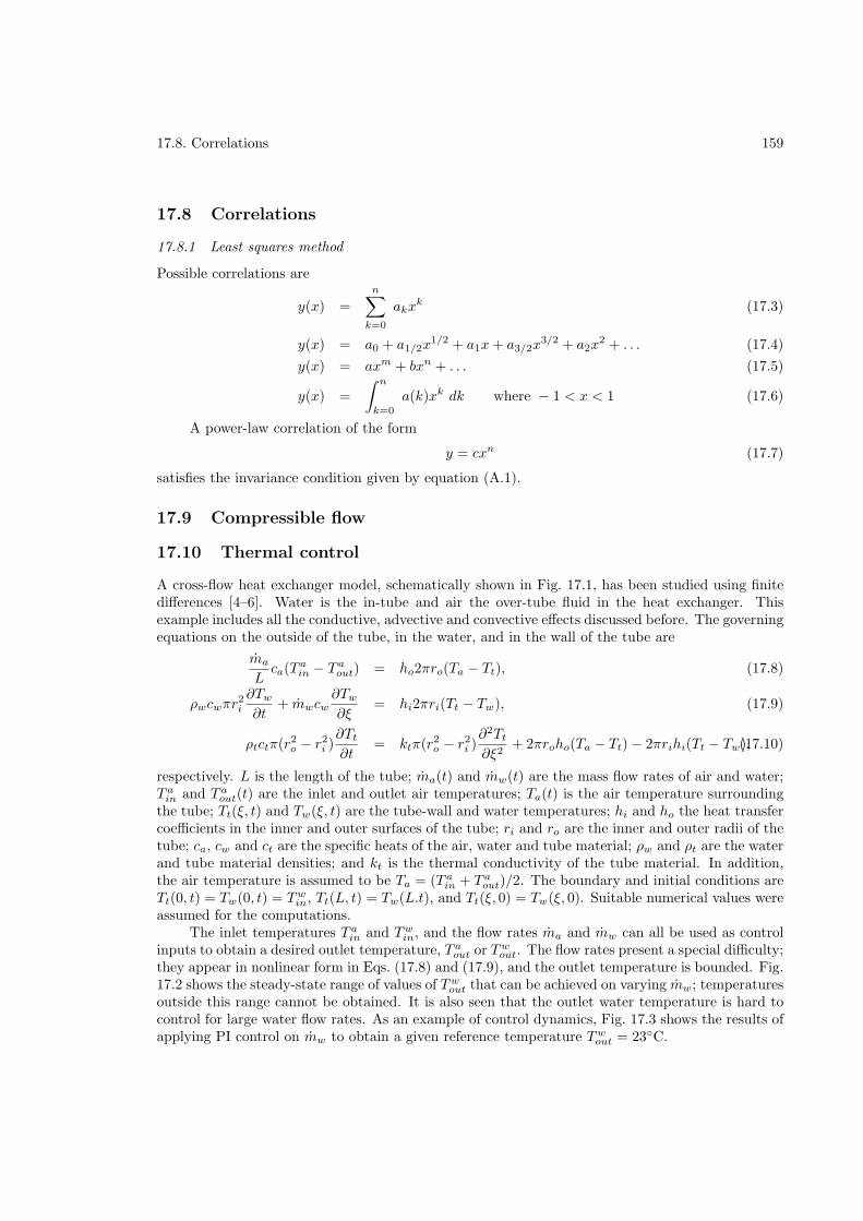
17.8. Correlations 159
17.8 Correlations
17.8.1 Least squares method
Possible correlations are
y(x) =
n∑
k=0
akxk (17.3)
y(x) = a0 + a1/2x1/2 + a1x+ a3/2x
3/2 + a2x2 + . . . (17.4)
y(x) = axm + bxn + . . . (17.5)
y(x) =
∫ n
k=0
a(k)xk dk where − 1 < x < 1 (17.6)
A power-law correlation of the form
y = cxn (17.7)
satisfies the invariance condition given by equation (A.1).
17.9 Compressible flow
17.10 Thermal control
A cross-flow heat exchanger model, schematically shown in Fig. 17.1, has been studied using finitedifferences [4–6]. Water is the in-tube and air the over-tube fluid in the heat exchanger. Thisexample includes all the conductive, advective and convective effects discussed before. The governingequations on the outside of the tube, in the water, and in the wall of the tube are
ma
Lca(T a
in − T aout) = ho2πro(Ta − Tt), (17.8)
ρwcwπr2i
∂Tw
∂t+ mwcw
∂Tw
∂ξ= hi2πri(Tt − Tw), (17.9)
ρtctπ(r2o − r2i )∂Tt
∂t= ktπ(r2o − r2i )
∂2Tt
∂ξ2+ 2πroho(Ta − Tt) − 2πrihi(Tt − Tw),(17.10)
respectively. L is the length of the tube; ma(t) and mw(t) are the mass flow rates of air and water;T a
in and T aout(t) are the inlet and outlet air temperatures; Ta(t) is the air temperature surrounding
the tube; Tt(ξ, t) and Tw(ξ, t) are the tube-wall and water temperatures; hi and ho the heat transfercoefficients in the inner and outer surfaces of the tube; ri and ro are the inner and outer radii of thetube; ca, cw and ct are the specific heats of the air, water and tube material; ρw and ρt are the waterand tube material densities; and kt is the thermal conductivity of the tube material. In addition,the air temperature is assumed to be Ta = (T a
in + T aout)/2. The boundary and initial conditions are
Tt(0, t) = Tw(0, t) = Twin, Tt(L, t) = Tw(L.t), and Tt(ξ, 0) = Tw(ξ, 0). Suitable numerical values were
assumed for the computations.The inlet temperatures T a
in and Twin, and the flow rates ma and mw can all be used as control
inputs to obtain a desired outlet temperature, T aout or Tw
out. The flow rates present a special difficulty;they appear in nonlinear form in Eqs. (17.8) and (17.9), and the outlet temperature is bounded. Fig.17.2 shows the steady-state range of values of Tw
out that can be achieved on varying mw; temperaturesoutside this range cannot be obtained. It is also seen that the outlet water temperature is hard tocontrol for large water flow rates. As an example of control dynamics, Fig. 17.3 shows the results ofapplying PI control on mw to obtain a given reference temperature Tw
out = 23C.
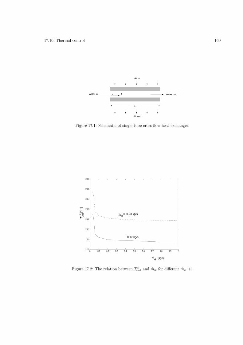
17.10. Thermal control 160
Water in
Air in
ξ
L
Water out
Air out
Figure 17.1: Schematic of single-tube cross-flow heat exchanger.
0 0.1 0.2 0.3 0.4 0.5 0.6 0.7 0.8 0.9 122.9
23
23.1
23.2
23.3
23.4
23.5
23.6
T [
°C]
ao
ut
[kg/s]ma.
= 0.23 kg/sma.
0.17 kg/s
Figure 17.2: The relation between T aout and mw for different ma [4].
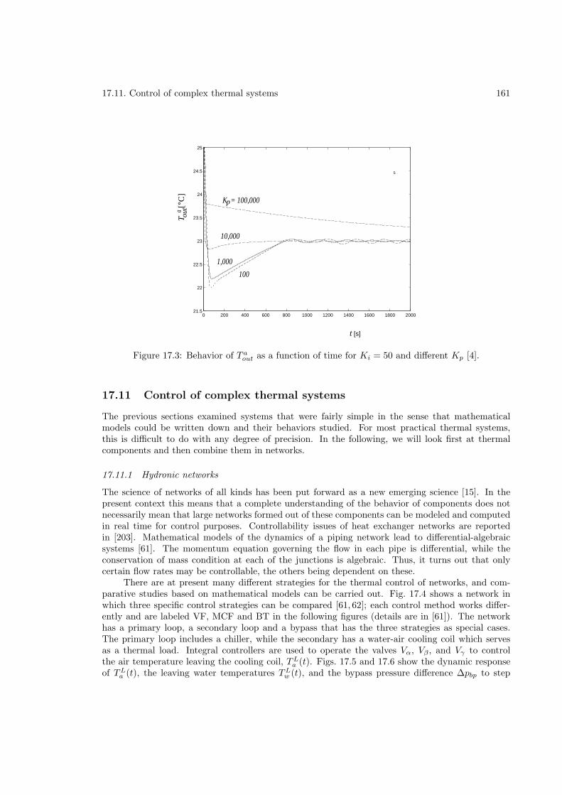
17.11. Control of complex thermal systems 161
0 200 400 600 800 1000 1200 1400 1600 1800 200021.5
22
22.5
23
23.5
24
24.5
25
t [s]
5
T
[°C
]a
ou
t
K = 100,000p
10,000
1,000
100
Figure 17.3: Behavior of T aout as a function of time for Ki = 50 and different Kp [4].
17.11 Control of complex thermal systems
The previous sections examined systems that were fairly simple in the sense that mathematicalmodels could be written down and their behaviors studied. For most practical thermal systems,this is difficult to do with any degree of precision. In the following, we will look first at thermalcomponents and then combine them in networks.
17.11.1 Hydronic networks
The science of networks of all kinds has been put forward as a new emerging science [15]. In thepresent context this means that a complete understanding of the behavior of components does notnecessarily mean that large networks formed out of these components can be modeled and computedin real time for control purposes. Controllability issues of heat exchanger networks are reportedin [203]. Mathematical models of the dynamics of a piping network lead to differential-algebraicsystems [61]. The momentum equation governing the flow in each pipe is differential, while theconservation of mass condition at each of the junctions is algebraic. Thus, it turns out that onlycertain flow rates may be controllable, the others being dependent on these.
There are at present many different strategies for the thermal control of networks, and com-parative studies based on mathematical models can be carried out. Fig. 17.4 shows a network inwhich three specific control strategies can be compared [61, 62]; each control method works differ-ently and are labeled VF, MCF and BT in the following figures (details are in [61]). The networkhas a primary loop, a secondary loop and a bypass that has the three strategies as special cases.The primary loop includes a chiller, while the secondary has a water-air cooling coil which servesas a thermal load. Integral controllers are used to operate the valves Vα, Vβ , and Vγ to controlthe air temperature leaving the cooling coil, TL
a (t). Figs. 17.5 and 17.6 show the dynamic responseof TL
a (t), the leaving water temperatures TLw (t), and the bypass pressure difference ∆pbp to step
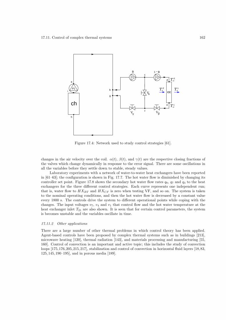
17.11. Control of complex thermal systems 162
P1
a
b
c
dP2 P3
Vγ
Vα
B
Vβ
− B1
e
f
g
h
i CC
ch
TaE Ta
L
TwL
TwE
Figure 17.4: Network used to study control strategies [61].
changes in the air velocity over the coil. α(t), β(t), and γ(t) are the respective closing fractions ofthe valves which change dynamically in response to the error signal. There are some oscillations inall the variables before they settle down to stable, steady values.
Laboratory experiments with a network of water-to-water heat exchangers have been reportedin [61–63]; the configuration is shown in Fig. 17.7. The hot water flow is diminished by changing itscontroller set point. Figure 17.8 shows the secondary hot water flow rates q8, q7 and q4 to the heatexchangers for the three different control strategies. Each curve represents one independent run;that is, water flow to HXBT and HXCF is zero when testing VF, and so on. The system is takento the nominal operating conditions, and then the hot water flow is decreased by a constant valueevery 1800 s. The controls drive the system to different operational points while coping with thechanges. The input voltages v7, v4 and v1 that control flow and the hot water temperature at theheat exchanger inlet T21 are also shown. It is seen that for certain control parameters, the systemis becomes unstable and the variables oscillate in time.
17.11.2 Other applications
There are a large number of other thermal problems in which control theory has been applied.Agent-based controls have been proposed by complex thermal systems such as in buildings [213],microwave heating [120], thermal radiation [143], and materials processing and manufacturing [55,160]. Control of convection is an important and active topic; this includes the study of convectionloops [175,176,205,215,217], stabilization and control of convection in horizontal fluid layers [18,83,125,145,190–195], and in porous media [189].
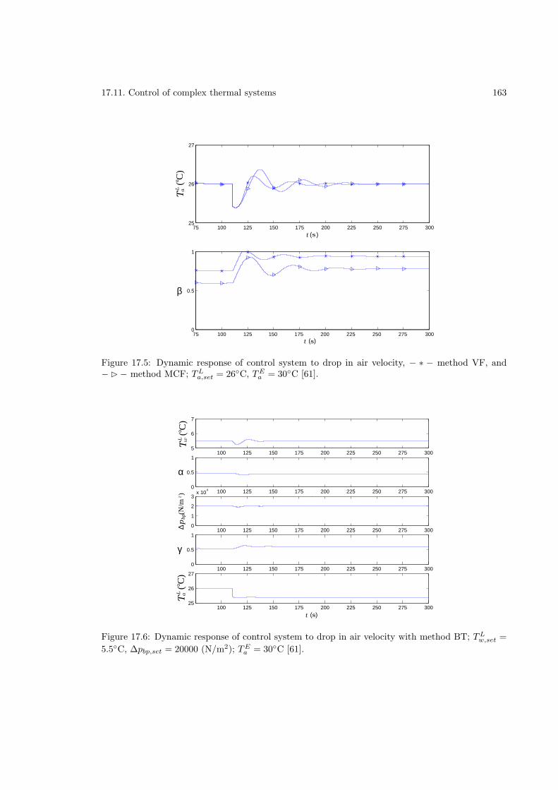
17.11. Control of complex thermal systems 163
75 100 125 150 175 200 225 250 275 30025
26
27
75 100 125 150 175 200 225 250 275 3000
0.5
1
TaL
o ( C
)
β
t (s)
t (s )
Figure 17.5: Dynamic response of control system to drop in air velocity, − ∗ − method VF, and− − method MCF; TL
a,set = 26C, TEa = 30C [61].
100 125 150 175 200 225 250 275 3005
6
7
t
100 125 150 175 200 225 250 275 3000
0.5
1
t
100 125 150 175 200 225 250 275 3000
1
2
3x 10
4
t
100 125 150 175 200 225 250 275 3000
0.5
1
t
100 125 150 175 200 225 250 275 30025
26
27
t (s)
γ
∆p
bp(N
/m )2
TwL
o ( C
)
α
TaL
o ( C
)
Figure 17.6: Dynamic response of control system to drop in air velocity with method BT; TLw,set =
5.5C, ∆pbp,set = 20000 (N/m2); TEa = 30C [61].
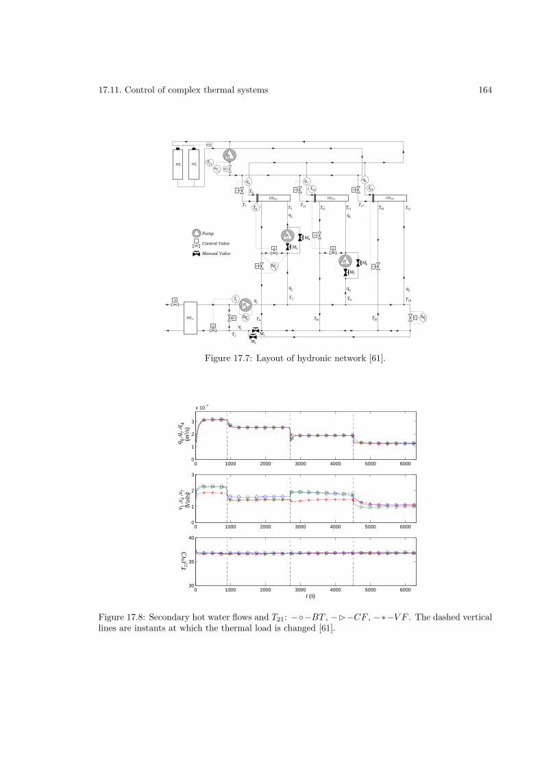
17.11. Control of complex thermal systems 164
HXm
13
HXBT HXCF HXVF
12
11
9
8
7
3
4
5
6
1
2
Pump
Control Valve
Manual Valve
HT1HT2
10
PID
T1
T21
T6 T5
T8
T7 T12 T11
T14
T12 T16 T15
T18
T17
T3
T4
T9 T19
T10 T20
P3
P2
q1
q1
q4
q7
q8
q3 q
6
P1
∆pV8
∆pP4
∆pV10
q2 q
5 q9
∆pV3
P4
T2 M1
M2
M3
M4
M5
M6
Figure 17.7: Layout of hydronic network [61].
0 1000 2000 3000 4000 5000 60000
1
2
3
x 10−4
0 1000 2000 3000 4000 5000 60000
1
2
3
0 1000 2000 3000 4000 5000 600030
35
40
T 21
C(
)
o
t s( )
v ,v
,v
V
olts
(
)
14
7q
,q
,q
(
)m
/s
38
74
Figure 17.8: Secondary hot water flows and T21: −−BT , −−CF , −∗−V F . The dashed verticallines are instants at which the thermal load is changed [61].
17.12. Conclusions 165
17.12 Conclusions
This has been a very brief introduction to the theory of thermal control. The fundamental ideas inthis subject are firmly grounded on the mathematics of systems and control theory which should bethe starting point. There are, however, a few aspects that are particularly characteristic of thermalsystems. Phenomena such as diffusion, convection and advection are common and the systemsare usually complex, nonlinear and poorly predictable dynamically. The governing equations covera wide range of possibilities, from ordinary and partial differential equations to functional anddifferential-algebraic systems. Furthermore, control theory itself is a vast subject, with specializedbranches like optimal [79], robust [38], and stochastic control [37] that are well developed. Many ofthe tools in these areas find applications in thermal systems.
The study of thermal control will continue to grow from the point of view of fundamentals aswell as engineering applications. There are many outstanding problems and issues that need to beaddressed. To cite one specific example, networking between a large number of coupled componentswill become increasingly important; it is known that unexpected synchronization may result evenwhen multiple dynamical systems are coupled weakly [181]. It is hoped that the reader will usethis brief overview as a starting point for further study and apply control theory in other thermalapplications.
Problems
1. This is a problem
Chapter 18
Soft computing
18.1 Genetic algorithms
[141]
18.2 Artificial neural networks
18.2.1 Heat exchangers
The most important of the components are heat exchangers, which are generally very complex in thatthey cannot be realistically computed in real time for control purposes [92, 153, 182]. An approachthat is becoming popular in these cases is that of artificial neural networks (ANN) [73] for predictionof system behavior both for time-independent [48,139,140,142] and time-dependent operation. It isparticularly suitable for systems for which experimental information that can be used for trainingis available. Reviews of artificial neural network applications to thermal engineering [163, 168] andother soft control methodologies [32,131,220] and applications [216] are available.
A stabilized neurocontrol technique for heat exchangers has been described in [47,49–52]. Fig.18.1 shows the test facility in which the experiments were conducted. The objective is to controlthe outlet air temperature T a
out. Figs. 18.2 shows the results of using neurocontrol compared withPID; both are effective. Fig. 18.3 shows the result of an disturbance rejection experiment. Theheat exchanger is stabilized at T a
out = 36C, and then the water flow is shut down between t = 40sand t = 70s; after that the neurocontroller brings the system back to normal operation. A neuralnetwork-based controller is able to adapt easily to changing circumstances; in thermal systemsthis may come from effects such as the presence of fouling over time or from changes in systemconfiguration as could happen in building heating and cooling systems.
[51,166][162]
Problems
1. This is a problem
166
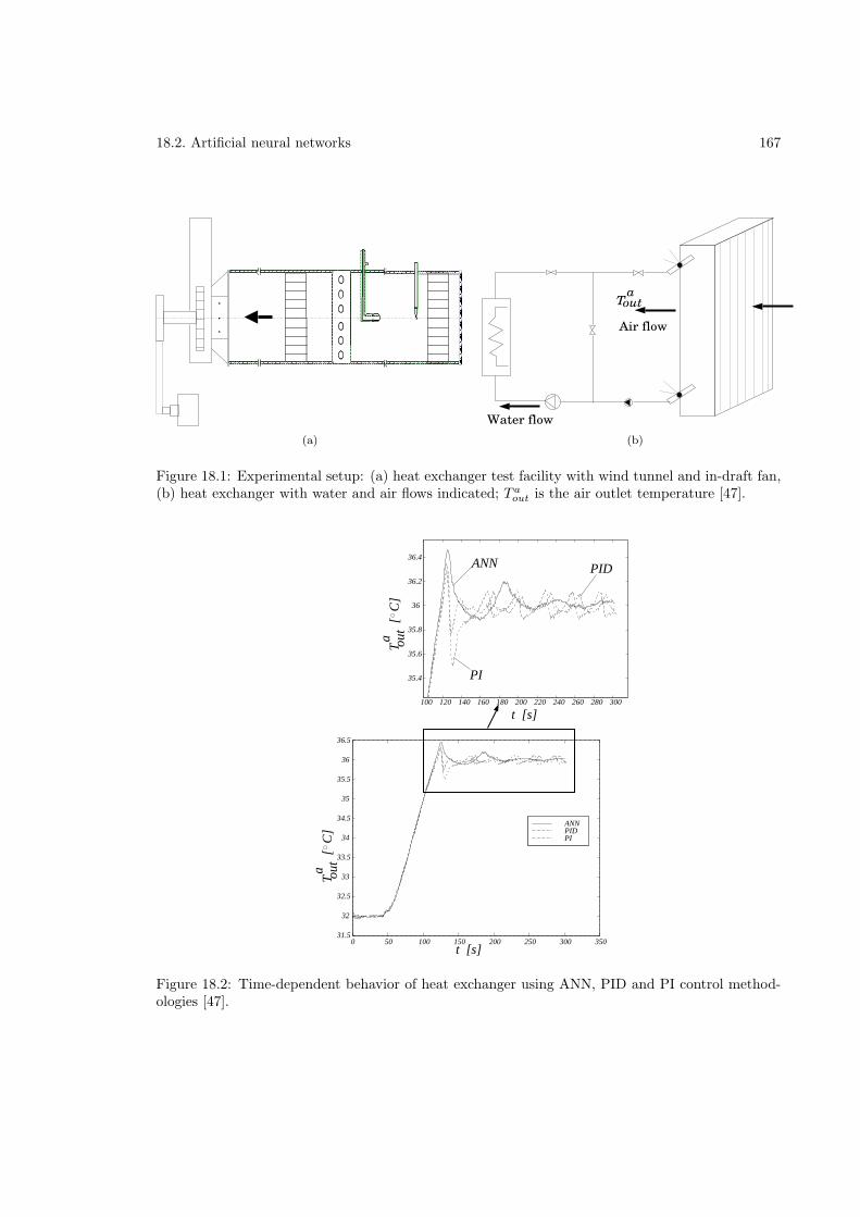
18.2. Artificial neural networks 167
(a)
Air flow
aTout
Water flow
(b)
Figure 18.1: Experimental setup: (a) heat exchanger test facility with wind tunnel and in-draft fan,(b) heat exchanger with water and air flows indicated; T a
out is the air outlet temperature [47].
0 50 100 150 200 250 300 35031.5
32
32.5
33
33.5
34
34.5
35
35.5
36
36.5
ANNPIDPI
100 120 140 160 180 200 220 240 260 280 300
35.4
35.6
35.8
36
36.2
36.4ANN
PI
PID
t [s]
T
[ C
]a ou
t
T
[ C
]a ou
t
t [s]
Figure 18.2: Time-dependent behavior of heat exchanger using ANN, PID and PI control method-ologies [47].
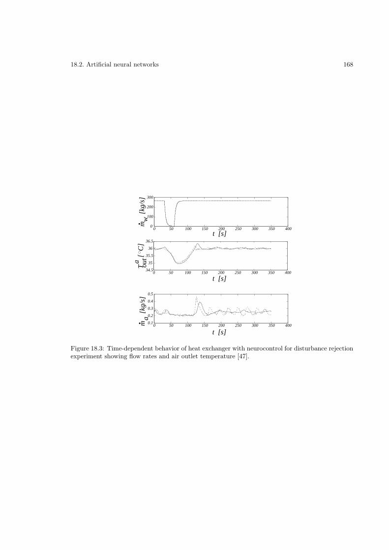
18.2. Artificial neural networks 168
0 50 100 150 200 250 300 350 4000
100
200
300
0 50 100 150 200 250 300 350 40034.5
35
35.5
36
36.5
0 50 100 150 200 250 300 350 4000.1
0.2
0.3
0.4
0.5
t [s]
t [s]
t [s]
am
[k
g/s
]m
[k
g/s
]w
T [ C
]o
ut
a
Figure 18.3: Time-dependent behavior of heat exchanger with neurocontrol for disturbance rejectionexperiment showing flow rates and air outlet temperature [47].

Part VI
Appendices
169
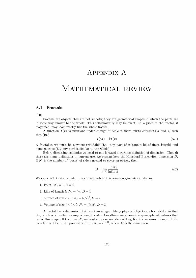
Appendix A
Mathematical review
A.1 Fractals
[60]Fractals are objects that are not smooth; they are geometrical shapes in which the parts are
in some way similar to the whole. This self-similarity may be exact, i.e. a piece of the fractal, ifmagnified, may look exactly like the whole fractal.
A function f(x) is invariant under change of scale if there exists constants a and b, suchthat [199]
f(ax) = bf(x) (A.1)
A fractal curve must be nowhere rectifiable (i.e. any part of it cannot be of finite length) andhomogeneous (i.e. any par6 is similar to the whole).
Before discussing examples we need to put forward a working definition of dimension. Thoughthere are many definitions in current use, we present here the Hausdorff-Besicovitch dimension D.If Nǫ is the number of ‘boxes’ of side ǫ needed to cover an object, then
D = limǫ→0
lnNǫ
ln(1/ǫ)(A.2)
We can check that this definition corresponds to the common geometrical shapes.
1. Point: Nǫ = 1,D = 0
2. Line of length l: Nǫ = l/ǫ,D = 1
3. Surface of size l × l: Nǫ = (l/ǫ)2,D = 2
4. Volume of size l × l × l: Nǫ = (l/ǫ)3,D = 3
A fractal has a dimension that is not an integer. Many physical objects are fractal-like, in thatthey are fractal within a range of length scales. Coastlines are among the geographical features thatare of this shape. If there are Nǫ units of a measuring stick of length ǫ, the measured length of thecoastline will be of the power-law form ǫNǫ = ǫ1−D, where D is the dimension.
170
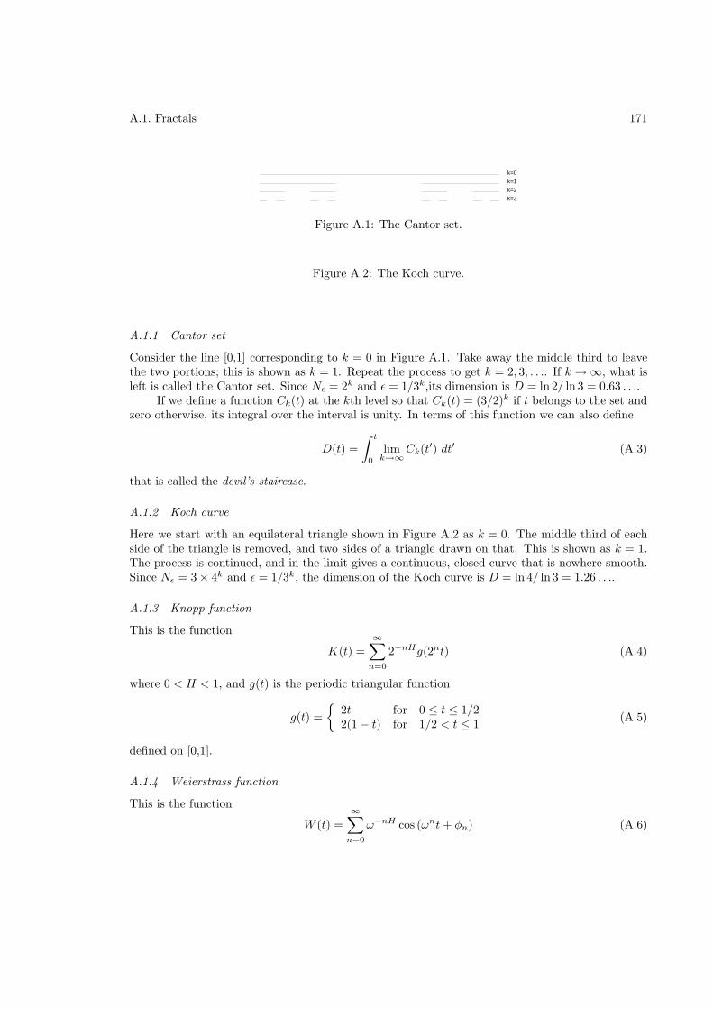
A.1. Fractals 171
k=0
k=1
k=2
k=3
Figure A.1: The Cantor set.
Figure A.2: The Koch curve.
A.1.1 Cantor set
Consider the line [0,1] corresponding to k = 0 in Figure A.1. Take away the middle third to leavethe two portions; this is shown as k = 1. Repeat the process to get k = 2, 3, . . .. If k → ∞, what isleft is called the Cantor set. Since Nǫ = 2k and ǫ = 1/3k,its dimension is D = ln 2/ ln 3 = 0.63 . . ..
If we define a function Ck(t) at the kth level so that Ck(t) = (3/2)k if t belongs to the set andzero otherwise, its integral over the interval is unity. In terms of this function we can also define
D(t) =
∫ t
0
limk→∞
Ck(t′) dt′ (A.3)
that is called the devil’s staircase.
A.1.2 Koch curve
Here we start with an equilateral triangle shown in Figure A.2 as k = 0. The middle third of eachside of the triangle is removed, and two sides of a triangle drawn on that. This is shown as k = 1.The process is continued, and in the limit gives a continuous, closed curve that is nowhere smooth.Since Nǫ = 3 × 4k and ǫ = 1/3k, the dimension of the Koch curve is D = ln 4/ ln 3 = 1.26 . . ..
A.1.3 Knopp function
This is the function
K(t) =
∞∑
n=0
2−nHg(2nt) (A.4)
where 0 < H < 1, and g(t) is the periodic triangular function
g(t) =
2t for 0 ≤ t ≤ 1/22(1 − t) for 1/2 < t ≤ 1
(A.5)
defined on [0,1].
A.1.4 Weierstrass function
This is the function
W (t) =∞∑
n=0
ω−nH cos (ωnt+ φn) (A.6)
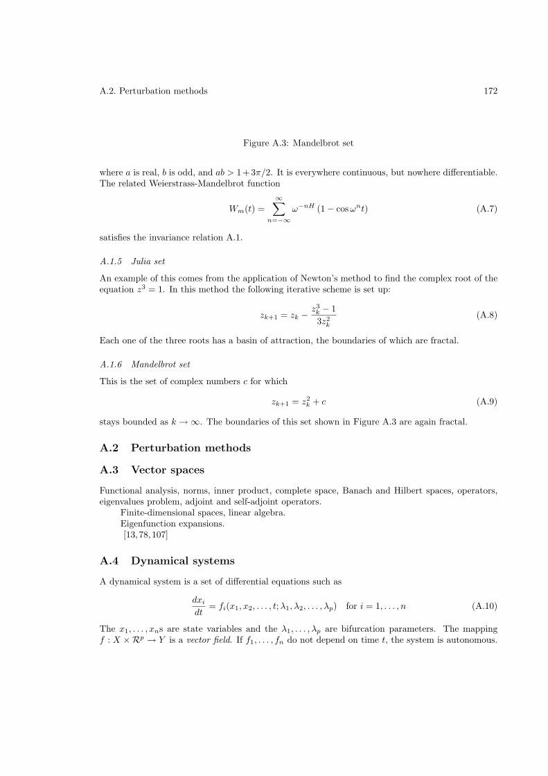
A.2. Perturbation methods 172
Figure A.3: Mandelbrot set
where a is real, b is odd, and ab > 1+3π/2. It is everywhere continuous, but nowhere differentiable.The related Weierstrass-Mandelbrot function
Wm(t) =
∞∑
n=−∞
ω−nH (1 − cosωnt) (A.7)
satisfies the invariance relation A.1.
A.1.5 Julia set
An example of this comes from the application of Newton’s method to find the complex root of theequation z3 = 1. In this method the following iterative scheme is set up:
zk+1 = zk − z3k − 1
3z2k
(A.8)
Each one of the three roots has a basin of attraction, the boundaries of which are fractal.
A.1.6 Mandelbrot set
This is the set of complex numbers c for which
zk+1 = z2k + c (A.9)
stays bounded as k → ∞. The boundaries of this set shown in Figure A.3 are again fractal.
A.2 Perturbation methods
A.3 Vector spaces
Functional analysis, norms, inner product, complete space, Banach and Hilbert spaces, operators,eigenvalues problem, adjoint and self-adjoint operators.
Finite-dimensional spaces, linear algebra.Eigenfunction expansions.[13,78,107]
A.4 Dynamical systems
A dynamical system is a set of differential equations such as
dxi
dt= fi(x1, x2, . . . , t;λ1, λ2, . . . , λp) for i = 1, . . . , n (A.10)
The x1, . . . , xns are state variables and the λ1, . . . , λp are bifurcation parameters. The mappingf : X ×Rp → Y is a vector field. If f1, . . . , fn do not depend on time t, the system is autonomous.
A.4. Dynamical systems 173
A nonautonomous system can be converted into autonomous one by the change in variable xn+1 = t,from which we can get the additional equation
dxn+1
dt= 1 (A.11)
We will assume that the solutions of the system are always bounded. The system is conservative ifthe divergence of the vector field
∑∂fi/∂xi is zero, and dissipative if it is negative. An attractor of
a dissipative dynamical system is the set of xi as t→ ∞. The critical (or singular, equilibrium orfixed) points, xi, of equation (A.10) are those for which
fi(x1, x2, . . . , t;λ1, λ2, . . . , λp) = 0 (A.12)
There may be multiple solutions to this algebraic or transcendental equation.Defining a new coordinate x′i = xi − xi that is centered at the critical point, we get the local
formdx′idt
= fi(x1 − x1, . . . , xn − xn) (A.13)
Sometimes we will use the notation
dxi
dt= g(x1, . . . , xn) (A.14)
to indicate the local form, the origin being one critical point of this system.
A.4.1 Stability
The stability of the critical points is of major interest. A critical point is stable if, given an initialperturbation, the solutions tends to it as t→ ∞.
Linear stability
The vector field in equation (A.14) can be expanded in a Taylor series to give
dxi
dt=∑
j
∂gi
∂xj
∣∣∣∣∣0
xj + . . . (A.15)
The eigenvalues of the Jacobian matrix
A =∂gi
∂xj(A.16)
determine the linear stability of the critical point. The critical point is stable if all eigenvalues havenegative real parts, and unstable if one or more eigenvalues have positive real parts.
A.4.2 Routh-Hurwitz criteria
The polynomial equationa0s
n + a1sn−1 + . . .+ an−1s+ an = 0
has roots with negative real parts if and only if the following conditions are satisfied:(i) a1/a0, a2/a0, . . . , an/a0 > 0(ii) Di > 0, i = 1, . . . , n
A.4. Dynamical systems 174
The Hurwitz determinants Di are defined by
D1 = a1
D2 =
∣∣∣∣a1 a3
a0 a2
∣∣∣∣
D3 =
∣∣∣∣∣∣
a1 a3 a5
a0 a2 a4
0 a1 a3
∣∣∣∣∣∣
Dn =
∣∣∣∣∣∣∣∣∣∣∣∣∣
a1 a3 a5 . . . a2n−1
a0 a2 a4 . . . a2n−2
0 a1 a3 . . . a2n−3
0 a0 a2 . . . a2n−4
......
......
...0 0 0 . . . an
∣∣∣∣∣∣∣∣∣∣∣∣∣
with ai = 0, if i > n.
Global stability
Consider the dynamical system in local form, equation (A.14). If there exists a function V (x1, . . . , xn)such that V ≥ 0 and dV/dt ≤ 0, then the origin is globally stable, that is, it is stable to allperturbations, large or small. V is called a Liapunov function.
[56]
A.4.3 Bifurcations
The critical point is one possible attractor. There are other time-dependent solutions which can alsobe attractors in phase space, as indicated in the list below.
• Point (steady, time-independent)
• Closed curve (limit cycle, periodic)
• Torus (periodic or quasi-periodic)
• Strange (chaotic)
For a given dynamical system, several attractors may co-exist. In this case each attractor hasa basin of attraction, i.e. the set of initial conditions that lead to this attractor. A bifurcation is aqualitative change in the solution as the bifurcation parameters λi are changed.
A.4.4 One-dimensional systems
A one-dimensional dynamical system is of the type
dx
dt= f(x) (A.17)
Example A.1Consider the linear equation
dx
dt= ax + b (A.18)
A.4. Dynamical systems 175
The critical point is
x = − b
a(A.19)
On defining x′ = x − x, the local form is obtained as
dx′
dt= ax′ (A.20)
We can take one of two approaches.
(a) Solvingx′ = x′
0eat (A.21)
The critical point is a repeller if a > 0, and an attractor if a < 0.
(b) Alternatively, we can multiply equation (A.20) by 2x′ to get
dV
dt= 2aV (A.22)
where V = x′2. Since V is always nonnegative, the sign of dV/dt is the sign of a. Thus V will increase withtime if a > 0, and decrease if a < 0.
In either case we find that the critical point is unstable if a > 0 and stable if a < 0.
Example A.2The nonlinear equation
dx
dt= −x
ˆ
x2 − (λ − λ0)˜
(A.23)
has critical point which are solutions of the cubic equation
xˆ
x2 − (λ − λ0)˜
= 0 (A.24)
Thus
x(1) = 0 (A.25)
x(2) =p
λ − λ0 (A.26)
x(3) = −p
λ − λ0 (A.27)
where x(i) (i = 1, 2, 3) are the three critical points. The bifurcation diagram is shown in Fig. A.4.
(i) Critical point x(1) = 0To analyze the local stability of x(1) = 0, we obtain the local form
dx′
dt= x′(λ − λ0) − x′3 (A.28)
Neglecting the cubic term x′3, this becomes
dx′
dt= x′(λ − λ0) (A.29)
Thus x(1) = 0 is locally stable if λ < λ0, and unstable if λ > λ0.To analyze the global stability, equation (A.28) can be written as
1
2
dV
dt= V (λ − λ0) − V 2 (A.30)
where V = x′2. For λ < λ0, V ≥ 0, dV/dt ≤ 0, so that x(1) = 0 is globally stable.
(ii) Critical point x(2) =√
λ − λ0
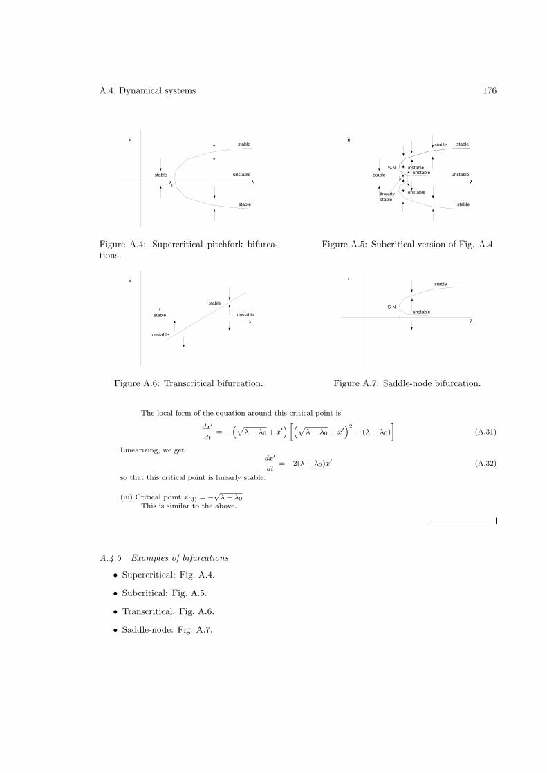
A.4. Dynamical systems 176
x
λλ0
unstablestable
stable
stable
Figure A.4: Supercritical pitchfork bifurca-tions
x
λ
unstable
stable
S-N
x
λunstablestable
stable
stable
unstable
unstablelinearlystable
Figure A.5: Subcritical version of Fig. A.4
x
λ
unstable
stable
stable
unstable
Figure A.6: Transcritical bifurcation.
x
λ
unstable
stable
S-N
Figure A.7: Saddle-node bifurcation.
The local form of the equation around this critical point is
dx′
dt= −
“
p
λ − λ0 + x′
”
»
“
p
λ − λ0 + x′
”2− (λ − λ0)
–
(A.31)
Linearizing, we getdx′
dt= −2(λ − λ0)x′ (A.32)
so that this critical point is linearly stable.
(iii) Critical point x(3) = −√
λ − λ0
This is similar to the above.
A.4.5 Examples of bifurcations
• Supercritical: Fig. A.4.
• Subcritical: Fig. A.5.
• Transcritical: Fig. A.6.
• Saddle-node: Fig. A.7.
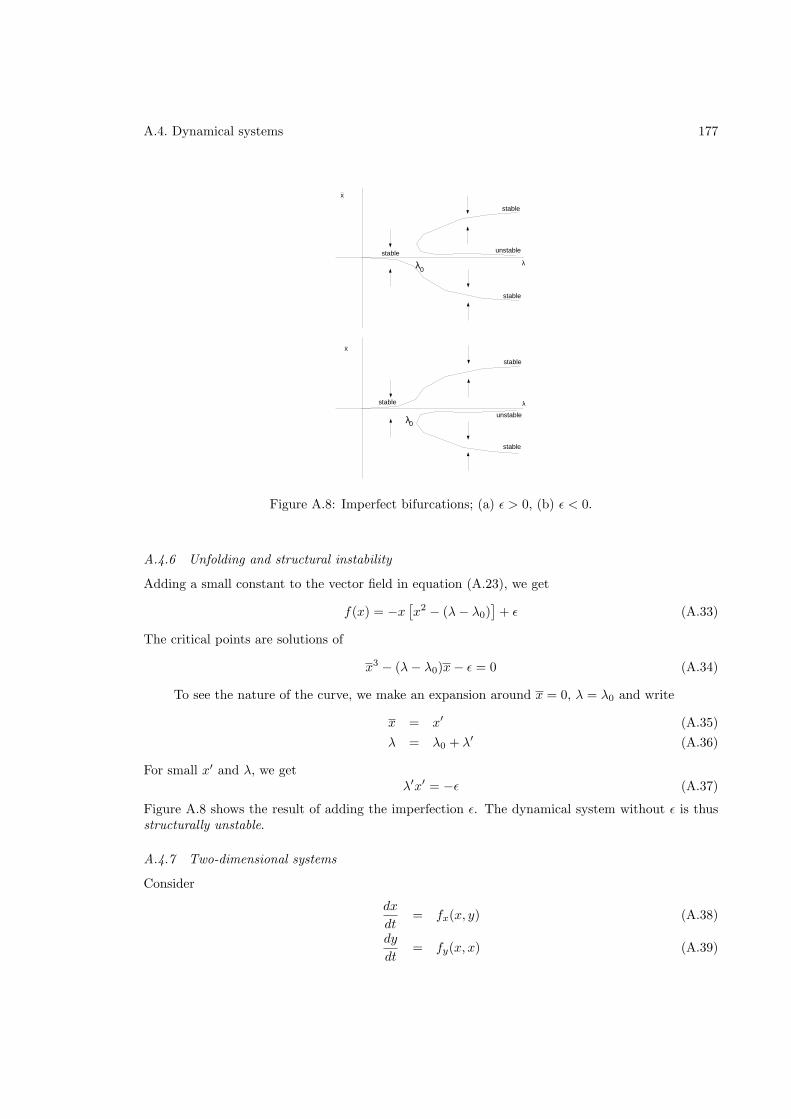
A.4. Dynamical systems 177
λ
unstable
stable
stable
stable
λ
unstablestable
stable
stable
x
x
λ0
λ0
Figure A.8: Imperfect bifurcations; (a) ǫ > 0, (b) ǫ < 0.
A.4.6 Unfolding and structural instability
Adding a small constant to the vector field in equation (A.23), we get
f(x) = −x[x2 − (λ− λ0)
]+ ǫ (A.33)
The critical points are solutions of
x3 − (λ− λ0)x− ǫ = 0 (A.34)
To see the nature of the curve, we make an expansion around x = 0, λ = λ0 and write
x = x′ (A.35)
λ = λ0 + λ′ (A.36)
For small x′ and λ, we getλ′x′ = −ǫ (A.37)
Figure A.8 shows the result of adding the imperfection ǫ. The dynamical system without ǫ is thusstructurally unstable.
A.4.7 Two-dimensional systems
Consider
dx
dt= fx(x, y) (A.38)
dy
dt= fy(x, x) (A.39)
A.4. Dynamical systems 178
The linearized equation in local form has a Jacobian matrix
A =
(axx axy
ayx ayy
)(A.40)
The eigenvalues satisfy a quadratic equation
λ2 + Pλ+Q = 0 (A.41)
from which
λ =1
2
[−P ±
√P 2 − 4Q
](A.42)
The sign of the discriminantD = P 2 − 4Q (A.43)
determines the nature of the solution. If D < 0, the eigenvalues are complex and the solution inphase space is a spiral; if in addition P > 0, the spiral is stable, and if P < 0, it is unstable. If,on the other hand, D > 0, the eigenvalues are real; the solutions do not oscillate in time but moveexponentially towards (if all eigenvalues are negative) or away (if at least one eigenvalue is positive)from the critical point.
Example A.3
dx
dt= y (A.44)
dy
dt= −(λ − λ0)x (A.45)
This is a conservative system which is equivalent to
d2x
dt2+ (λ − λ0)x = 0 (A.46)
The solutions are exponential if λ < λ0, and periodic if λ > λ0.
Example A.4
dx
dt= y (A.47)
dy
dt= −ω2x − σy (A.48)
For σ > 0, the system is dissipative, and the solutions are damped oscillations.
The occurrence of periodic solutions in two-dimensional systems, permits a Hopf bifurcation,which is a transition from a time-independent to a periodic behavior through a pair of complexconjugate imaginary eigenvalues.
A.4. Dynamical systems 179
Example A.5The dynamical system
dx
dt= (λ − λ0)x − y − (x2 + y2)x (A.49)
dy
dt= x + (λ − λ0)y − (x2 + y2)y (A.50)
can be converted to polar coordinates. Substituting x = r cos θ and y = r sin θ, we get
−r sindθ
dt+ cos θ
dr
dt= (λ − λ0)r cos θ − r sin θ − r3 cos θ (A.51)
r cosdθ
dt+ sin θ
dr
dt= r cos θ + (λ − λ0)r sin θ − r3 sin θ (A.52)
which simplifies to
dr
dt= r
`
λ − λ0 − r2´
(A.53)
dθ
dt= 1 (A.54)
There are two values of r, i..e r = 0 and r =√
λ − λ0, at which dr/dt = 0. The first is a critical point at theorigin, and the second a circular periodic orbit that exists only for λ > λ0. A linear analysis of equations (A.49)and (AHopftwo) shows that the origin is stable for λ < λ0. For λ > λ0, a similar analysis of equation (A.53)indicates that r =
√λ − λ0 is a stable orbit. There is thus a Hopf bifurcation at λ = λ0.
Example A.6
dx
dt= y (A.55)
dy
dt= −ω2x − σ
`
λ − x2 − y2´
(A.56)
This is a Hopf bifurcation at λ = λ0, at which point the solution goes from time-independent to periodic.
A.4.8 Three-dimensional systems
Forced Duffing equation
Since a non-autonomous equation can be converted into a three-dimensional autonomous system,we will include the case of the forced Duffing equation here1.
dx
dt= y (A.57)
dy
dt= x− x3 + f(t) (A.58)
1Sometimes defined with a negative sign in front of x in the second equation.
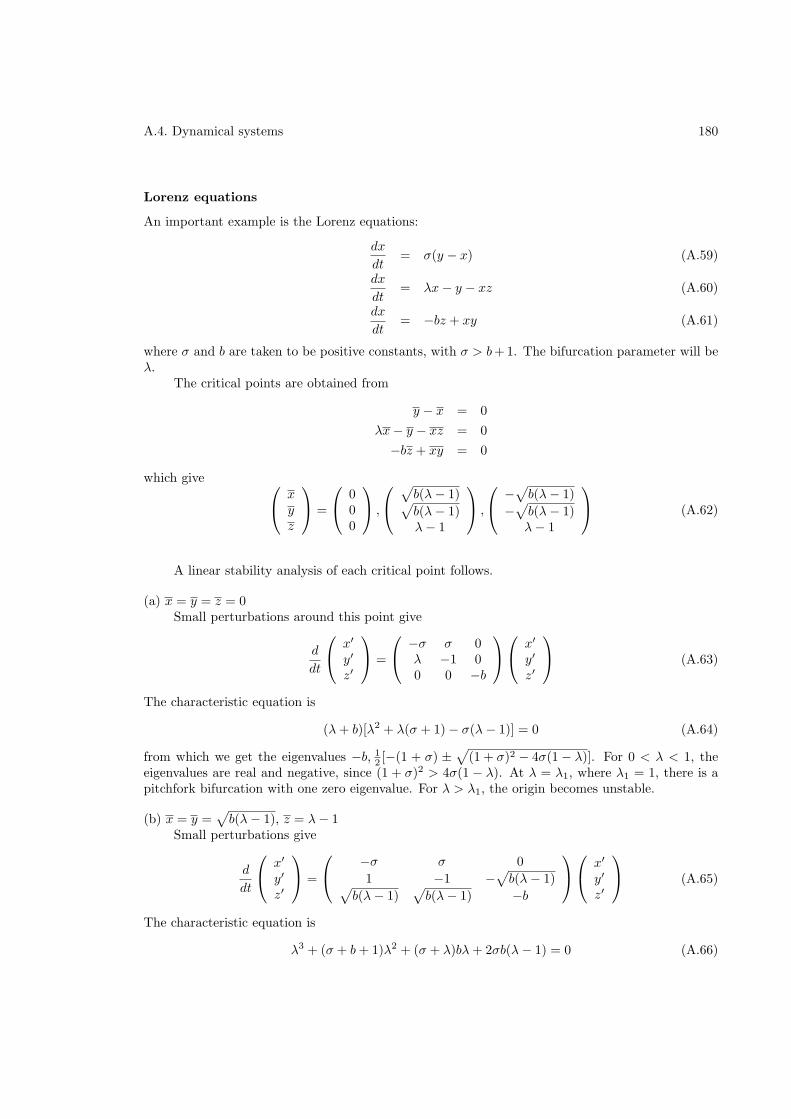
A.4. Dynamical systems 180
Lorenz equations
An important example is the Lorenz equations:
dx
dt= σ(y − x) (A.59)
dx
dt= λx− y − xz (A.60)
dx
dt= −bz + xy (A.61)
where σ and b are taken to be positive constants, with σ > b+ 1. The bifurcation parameter will beλ.
The critical points are obtained from
y − x = 0
λx− y − xz = 0
−bz + xy = 0
which give
xyz
=
000
,
√b(λ− 1)√b(λ− 1)λ− 1
,
−√b(λ− 1)
−√b(λ− 1)λ− 1
(A.62)
A linear stability analysis of each critical point follows.
(a) x = y = z = 0Small perturbations around this point give
d
dt
x′
y′
z′
=
−σ σ 0λ −1 00 0 −b
x′
y′
z′
(A.63)
The characteristic equation is
(λ+ b)[λ2 + λ(σ + 1) − σ(λ− 1)] = 0 (A.64)
from which we get the eigenvalues −b, 12 [−(1 + σ) ±
√(1 + σ)2 − 4σ(1 − λ)]. For 0 < λ < 1, the
eigenvalues are real and negative, since (1 + σ)2 > 4σ(1 − λ). At λ = λ1, where λ1 = 1, there is apitchfork bifurcation with one zero eigenvalue. For λ > λ1, the origin becomes unstable.
(b) x = y =√b(λ− 1), z = λ− 1
Small perturbations give
d
dt
x′
y′
z′
=
−σ σ 0
1 −1 −√b(λ− 1)√
b(λ− 1)√b(λ− 1) −b
x′
y′
z′
(A.65)
The characteristic equation is
λ3 + (σ + b+ 1)λ2 + (σ + λ)bλ+ 2σb(λ− 1) = 0 (A.66)
A.5. Singularity theory 181
Using the Hurwitz criteria we can determine the sign of the real parts of the solutions of this cubicequation without actually solving it. The Hurwitz determinants are
D1 = σ + b+ 1
D2 =
∣∣∣∣σ + b+ 1 2σb(λ+ 1)
1 (σ + λ)b
∣∣∣∣= σb(σ + b+ 3) − λb(σ − b− 1)
D3 =
∣∣∣∣∣∣
σ + b+ 1 2σb(λ− 1) 01 (σ + λ)b 00 σ + b+ 1 2σb(λ− 1)
∣∣∣∣∣∣= 2σb(λ− 1)[σb(σ + b+ 3) − λb(σ − b− 1)]
Thus the real parts of the eigenvalues are negative if λ < λ3, where
λ3 =σ(σ + b+ 3)
σ − b− 1(A.67)
At λ = λ3 the characteristic equation (A.66) can be factorized to give the eigenvalues −(σ + b+ 1),and ±i 2σ(σ + 1)/(σ − b− 1), corresponding to a Hopf bifurcation. The periodic solution which iscreated at this value of λ can be shown to be unstable so that the bifurcation is subcritical.
Here is a summary of the series of bifurcation with respect to the parameter λ:
• Origin is a stable critical point for λ < λ1; becomes unstable at λ = λ1.
• Two other critical points are created for λ > λ1; these are linearly stable in the range λ1 <λ < λ3.
• Just below λ3, i.e. in the range λ2 < λ < λ3, the two critical points are stable to smallperturbations, but for large enough perturbations produce chaos.
• For λ > λ3, all initial conditions produce chaos (except for periodic windows).
A.4.9 Nonlinear analysis
Center manifold theorem
[30]Consider a vector field fi(x) with fi(0) = 0. The eigenvalues λ of ∂fi/∂xj at the origin are of
three kinds:(a) Re(λ) > 0 with the generalized eigenspace Eu.(b) Re(λ) < 0 with the generalized eigenspace Es.(c) Re(λ) = 0 with the generalized eigenspace Ec.There exist manifolds Wu, W s, and W c to which Eu, Es and Ec, respectively, are tangents. Wu,W s, and W c are the unstable, stable and center manifolds, respectively.
A.5 Singularity theory
We have seen that the critical points of a dynamical system, equation (A.10), are found by solvingan equation of the type (A.12), i.e. by finding the singularities of the function fi. The type ofbifurcations that occur with a single bifurcation parameter λ has been discussed in the previous
A.6. Partial differential equations 182
x
λ
µ
Figure A.9: Surface x = x(λ, µ).
λ
µ
One solution
Three solutions
One solution
Figure A.10: Bifurcation set.
section. Here we increase the number of parameters to λ1, . . . , λp and look at the consequentchanges in the bifurcations. A bifurcation (or catastrophe) set is the set of points in parametricspace λ1, . . . , λp at which equation (A.12) is satisfied.
Example A.7Examine the one-dimensional vector field
f(x) = −(x3 + px + q) (A.68)
Figure A.9 shows the surface x = x(λ, µ). There are three real solutions if the discriminant D = 4λ3 +27µ2 > 0,and only one otherwise. A section of this surface at µ = 0 will give Fig. A.4 and µ = ǫ will give Fig. A.8.
The bifurcation set is shown in Fig. A.10 in (λ, µ) coordinates. It is projection of the x = x(λ, µ) surfacein the (λ, µ) plane.
The quadratic surface
a1x2 + a2y
2 + a3z3 + a4xy + a5xz + a6yz + a7x+ a8y + a9z + a10 = 0 (A.69)
can be classified in terms of eleven canonical surfaces. For gradient systems, i.e. systems in whichfI = ∂φ/∂xi, there are only seven.
A.6 Partial differential equations
ClassificationBoundary conditions
A.6.1 Eigenfunction expansion
Let T = T (x, t) and∂T
∂t= L(T ) (A.70)
in a domain Ω, where L is a linear operator with spatial partial derivatives. The boundary andinitial conditions are T = 0 at ∂Ω and T = f(x) at t = 0.
Let φi(x) be the eigenfunctions of L, such that
Lφi = λiφ. (A.71)
A.7. Waves 183
Expand T (x, t) in the form
T (x, t) =
∞∑
i=1
ai(t)φi(x). (A.72)
Substituting in the equation, we get
∞∑
i=1
dai
dtφi =
∞∑
i=1
ai(t)L(φi). (A.73)
Taking the inner product with φj , we find that
∞∑
i=1
dai
dt〈φi, φj〉 =
∞∑
i=1
ai(t)〈L(φi), φj〉. (A.74)
At this point we restrict ourselves to the special case in which L is a self-adjoint operator, so thatthe λi are real and the φi are orthonormal. Thus
〈φi, φj〉 = δij . (A.75)
Using eq. (A.71), we getdaj
dt= λjaj . (A.76)
A.7 Waves
A wave can be of the form [208]f(x, t) = Aei(kx−ωt). (A.77)
If we follow a point at constant phase φ = kx−ωt = k(x−ωt/k), we will be moving with the phasevelocity vp, where
vp =ω
k. (A.78)
The relation between the frequency ω and the wave number k
ω = ω(k) (A.79)
is called the dispersion relation. The group velocity is the velocity at which the energy of the wavemoves, and is given by
vg =dω
dk. (A.80)
Problems
1. Show thatdx
dt= −x [x − (λ − λ0)]
has a transcritical bifurcation.
2. Carry out an imperfection analysis on the transcritical bifurcation above.
3. Show thatdx
dt= −x2 + (λ − λ0)
has a saddle-node bifurcation.
4. Investigate the bifurcations indx
dt= −x
`
x4 − 2x2 + 2 + λ´
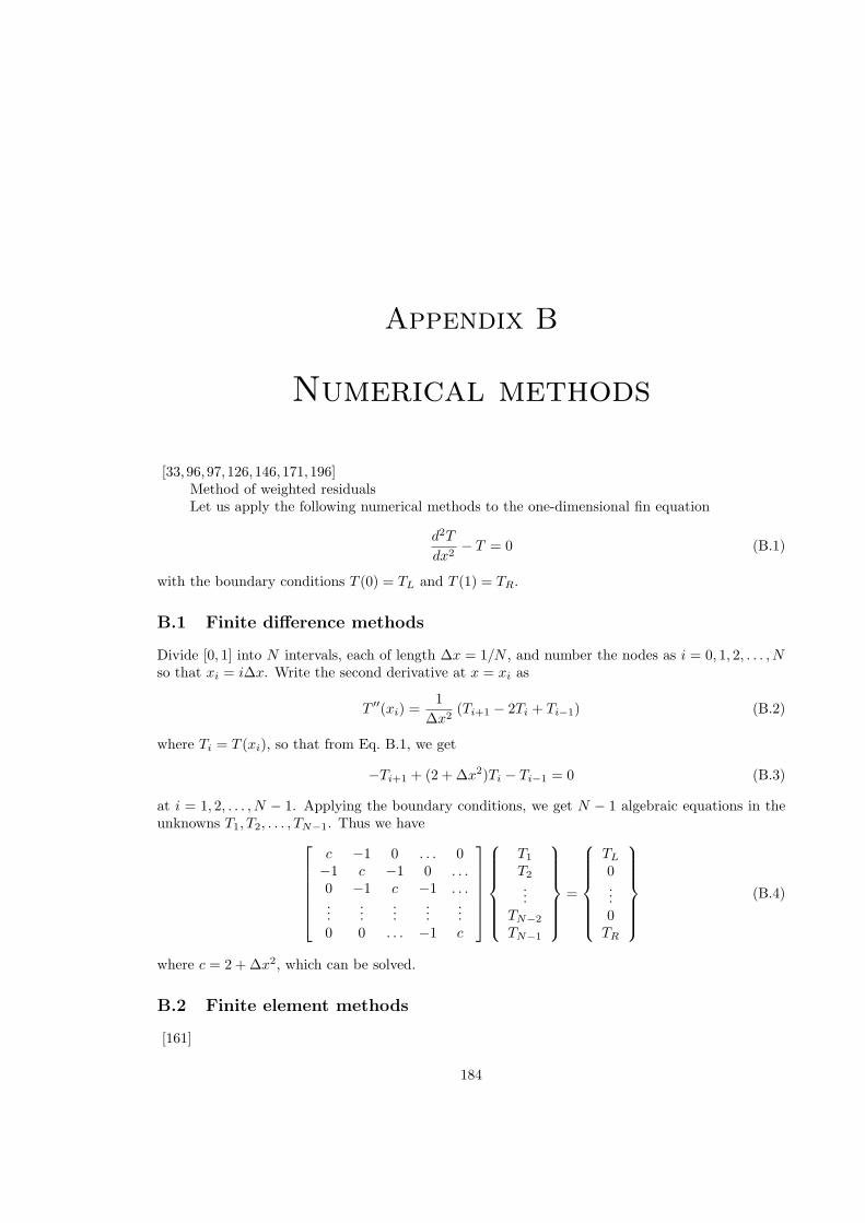
Appendix B
Numerical methods
[33, 96,97,126,146,171,196]Method of weighted residualsLet us apply the following numerical methods to the one-dimensional fin equation
d2T
dx2− T = 0 (B.1)
with the boundary conditions T (0) = TL and T (1) = TR.
B.1 Finite difference methods
Divide [0, 1] into N intervals, each of length ∆x = 1/N , and number the nodes as i = 0, 1, 2, . . . , Nso that xi = i∆x. Write the second derivative at x = xi as
T ′′(xi) =1
∆x2(Ti+1 − 2Ti + Ti−1) (B.2)
where Ti = T (xi), so that from Eq. B.1, we get
−Ti+1 + (2 + ∆x2)Ti − Ti−1 = 0 (B.3)
at i = 1, 2, . . . , N − 1. Applying the boundary conditions, we get N − 1 algebraic equations in theunknowns T1, T2, . . . , TN−1. Thus we have
c −1 0 . . . 0−1 c −1 0 . . .0 −1 c −1 . . ....
......
......
0 0 . . . −1 c
T1
T2
...TN−2
TN−1
=
TL
0...0TR
(B.4)
where c = 2 + ∆x2, which can be solved.
B.2 Finite element methods
[161]
184
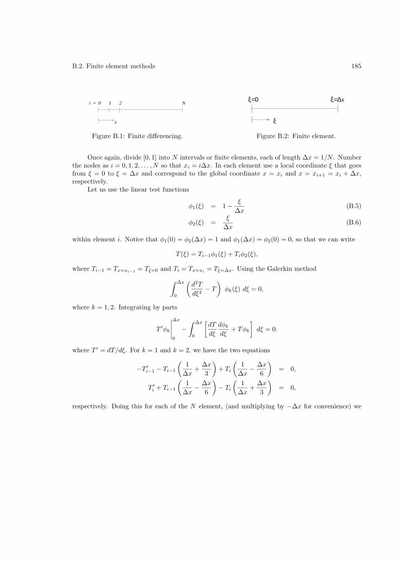
B.2. Finite element methods 185
1 2 N
x
i = 0
Figure B.1: Finite differencing.
ξ
ξ=0 ξ=∆x
Figure B.2: Finite element.
Once again, divide [0, 1] into N intervals or finite elements, each of length ∆x = 1/N . Numberthe nodes as i = 0, 1, 2, . . . , N so that xi = i∆x. In each element use a local coordinate ξ that goesfrom ξ = 0 to ξ = ∆x and correspond to the global coordinate x = xi and x = xi+1 = xi + ∆x,respectively.
Let us use the linear test functions
φ1(ξ) = 1 − ξ
∆x(B.5)
φ2(ξ) =ξ
∆x(B.6)
within element i. Notice that φ1(0) = φ2(∆x) = 1 and φ1(∆x) = φ2(0) = 0, so that we can write
T (ξ) = Ti−1φ1(ξ) + Tiφ2(ξ),
where Ti−1 = Tx=xi−1= Tξ=0 and Ti = Tx=xi
= Tξ=∆x. Using the Galerkin method
∫ ∆x
0
(d2T
dξ2− T
)φk(ξ) dξ = 0,
where k = 1, 2. Integrating by parts
T ′φk
∣∣∣∣∣
∆x
0
−∫ ∆x
0
[dT
dξ
dφk
dξ+ Tφk
]dξ = 0.
where T ′ = dT/dξ. For k = 1 and k = 2, we have the two equations
−T ′
i−1 − Ti−1
(1
∆x+
∆x
3
)+ Ti
(1
∆x− ∆x
6
)= 0,
T ′
i + Ti−1
(1
∆x− ∆x
6
)− Ti
(1
∆x+
∆x
3
)= 0,
respectively. Doing this for each of the N element, (and multiplying by −∆x for convenience) we
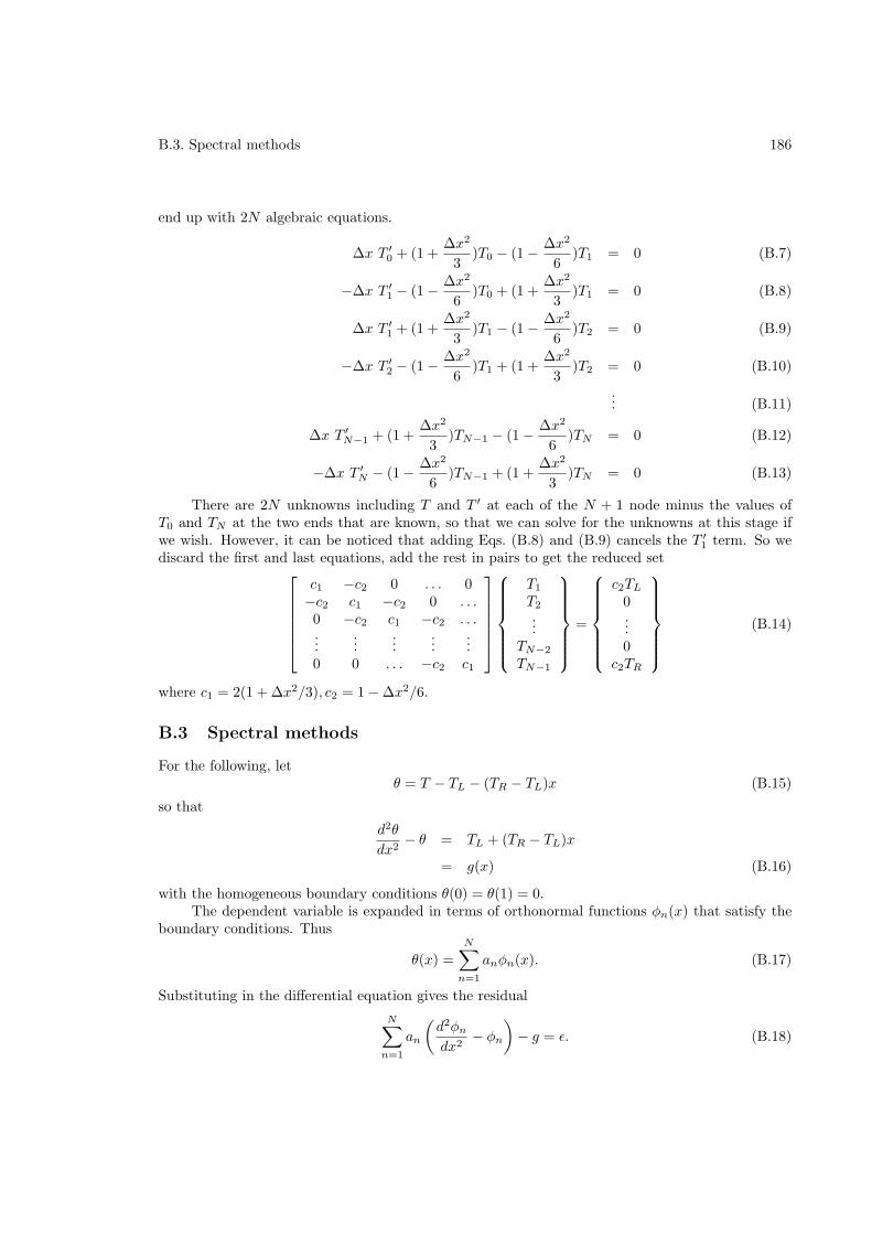
B.3. Spectral methods 186
end up with 2N algebraic equations.
∆x T ′
0 + (1 +∆x2
3)T0 − (1 − ∆x2
6)T1 = 0 (B.7)
−∆x T ′
1 − (1 − ∆x2
6)T0 + (1 +
∆x2
3)T1 = 0 (B.8)
∆x T ′
1 + (1 +∆x2
3)T1 − (1 − ∆x2
6)T2 = 0 (B.9)
−∆x T ′
2 − (1 − ∆x2
6)T1 + (1 +
∆x2
3)T2 = 0 (B.10)
... (B.11)
∆x T ′
N−1 + (1 +∆x2
3)TN−1 − (1 − ∆x2
6)TN = 0 (B.12)
−∆x T ′
N − (1 − ∆x2
6)TN−1 + (1 +
∆x2
3)TN = 0 (B.13)
There are 2N unknowns including T and T ′ at each of the N + 1 node minus the values ofT0 and TN at the two ends that are known, so that we can solve for the unknowns at this stage ifwe wish. However, it can be noticed that adding Eqs. (B.8) and (B.9) cancels the T ′
1 term. So wediscard the first and last equations, add the rest in pairs to get the reduced set
c1 −c2 0 . . . 0−c2 c1 −c2 0 . . .0 −c2 c1 −c2 . . ....
......
......
0 0 . . . −c2 c1
T1
T2
...TN−2
TN−1
=
c2TL
0...0
c2TR
(B.14)
where c1 = 2(1 + ∆x2/3), c2 = 1 − ∆x2/6.
B.3 Spectral methods
For the following, letθ = T − TL − (TR − TL)x (B.15)
so that
d2θ
dx2− θ = TL + (TR − TL)x
= g(x) (B.16)
with the homogeneous boundary conditions θ(0) = θ(1) = 0.The dependent variable is expanded in terms of orthonormal functions φn(x) that satisfy the
boundary conditions. Thus
θ(x) =
N∑
n=1
anφn(x). (B.17)
Substituting in the differential equation gives the residual
N∑
n=1
an
(d2φn
dx2− φn
)− g = ǫ. (B.18)
B.4. MATLAB 187
Making the residual and functions ψm(x) orthogonal gives
〈ǫ, ψm〉 = 0 (B.19)
This reduces to an algebraic equation for each m. Solve.
B.3.1 Trigonometric Galerkin
Hereφn(x) = ψn(x) =
√2 sin(nπx) (B.20)
with respect to the L2 inner product.
B.3.2 Trigonometric collocation
Equate the residual in Eq. (B.18) to zero in N equally-spaced points. This gives algebraic equations;solve.
B.3.3 Chebyshev Galerkin
Using ξ = 2x − 1, transform the independent variable to the domain [−1, 1]. The orthonormalChebychev functions are φn(ξ) = 2nTn(ξ)/
√2π, where the Chebychev polynomials Tn are
T1 = 1
T2 = ξ
T3 = 2ξ2 − 1
T4 = 4ξ3 − 3ξ
...
Take ψn(ξ) = φn(ξ) and an inner product with respect to the weight function 1/√
1 − ξ2.
B.3.4 Legendre Galerkin
B.3.5 Moments
Let φ(x) = x(1 − x), so that it satisfies the boundary conditions and θ(x) = aφ(x). Take ψ(x) = 1to determine a.
For higher-order accuracy, take φ1(x) = x(1− x), φ2(x) = x2(1− x), φ3(x) = x(1− x)2, . . . andψ1(x) = 1, ψ2(x) = x, ψ3(x) = x2, . . .
B.4 MATLAB
The PDE Toolbox uses a finite-element code to solve basic partial differential equations needed forconduction heat transfer.
B.4. MATLAB 188
Problems
1. Consider the convective fin equationd2T
dx2− T = 0,
where 0 ≤ x ≤ 1, with T (0) = 1, T (1) = 0. Solve using the following methods. You may have to transform thedependent or independent variable differently for each method. In each case show convergence.
(a) Finite differences: Divide into N parts, write derivatives in terms of finite differences, reduce to algebraicequations, apply boundary conditions, and solve.
(b) Trigonometric Galerkin: Expand in terms of N trigonometric functions, substitute in equation, takeinner products, reduce to algebraic equations, and solve.
(c) Chebyshev Galerkin: Expand in terms of N Chebyshev polynomials, substitute in equation, take innerproducts, reduce to algebraic equations, and solve.
(d) Trigonometric collocation: Expand in terms of N trigonometric functions, substitute in equation, takeinner products, apply collocation, and solve.
(e) Galerkin finite elements: Divide into N elements, assume linear functions, integrate by parts, assembleall equations, apply boundary conditions, and solve.
(f) Polynomial moments: Assume dependent variable to be a Nth-order polynomial that satisfies boundaryconditions, obtain algebraic equations by taking moments, and solve.
2. Consider the convective fin equation with heat generation
d2T
dx2− T = 1,
where 0 ≤ x ≤ 1, with T (0) = 1, T ′(1) = 0. Solve using the above methods.
Appendix C
Additional problems
1. Plot all real θ(β, ǫ) surfaces for the convection with radiation problem, and comment on theexistence of solutions.
2. Complete the problem of radiation in an enclosure (linear stability, numerical solutions).
3. Two bodies at temperatures T1(t) and T2(t), respectively, are in thermal contact with eachother and with the environment. The temperatures are governed by
M1c1dT1
dt+ hAc(T1 − T2) + hA(T1 − T∞) = 0 (C.1)
M2c2dT2
dt+ hAc(T2 − T1) + hA(T2 − T∞) = 0 (C.2)
Derive the equations above and explain the parameters. Find the steady-state temperaturesand explore the stability of the system for constant T∞.
4. Consider the change in temperature of a lumped system with convective heat transfer wherethe ambient temperature, T∞(t), varies with time in the form shown. Find (a) the long-timesolution of the system temperature, T (t), and (b) the amplitude of oscillation of the systemtemperature, T (t), for a small period δt.
t
T∞
Tmax
Tmin
δt
Figure C.1: Ambient temperature variation.
5. Two bodies at temperatures T1(t) and T2(t), respectively, are in thermal contact with each
189
190
other and with the environment. The temperatures are governed by
M1c1dT1
dt+ hcAc(T1 − T2) + hA(T1 − T∞(t)) = Q1(t)
M2c2dT2
dt+ hcAc(T2 − T1) + hA(T2 − T∞(t)) = Q2(t)
where Q1 and Q2 are internal heat generations, each one of which can be independentlycontrolled. Using PID control, show numerical results for the different types of responsespossible (damped, oscillatory, unstable, stable, etc.). Take the ambient temperature, T∞, tobe (a) constant and (b) oscillatory.
6. Two bodies at temperatures T1(t) and T2(t), respectively, are in thermal contact with eachother and with the environment. The temperatures are governed by
M1c1dT1
dt+ hcAc(T1 − T2) + hA(T1 − T∞(t)) = Q1(t)
M2c2dT2
dt+ hcAc(T2 − T1) + hA(T2 − T∞(t)) = Q2(t)
where Q1 and Q2 are internal heat generation sources, each one of which can be independentlycontrolled. Using on-off control, show analytical or numerical results for the temperatureresponses of the two bodies. If you do the problem analytically, take the ambient temperature,T∞, to be constant, but if you do it numerically, then you can take it to be (a) constant, and(b) oscillatory.
7. Consider a rectangular fin with convection, radiation and Dirichlet boundary conditions. Cal-culate numerically the evolution of an initial temperature distribution at different instants oftime. Graph the results for several values of the parameters.
8. Consider a longitudinal fin of concave parabolic profile as shown in the figure, where δ =[1− (x/L)]2δb. δb is the thickness of the fin at the base. Assume that the base temperature isknown. Neglect convection from the thin sides. Find (a) the temperature distribution in thefin, and (b) the heat flow at the base of the fin. Optimize the fin assuming the fin volume tobe constant and maximizing the heat rate at the base. Find (c) the optimum base thicknessδb, and (d) the optimum fin height L.
9. Analyze an annular fin with a prescribed base temperature and adiabatic tip. Determine itsfin efficiency and plot.
10. Consider a square plate of side 1 m. The temperatures on each side are (a) 10C, (b) 10C, (c)10C, and (d) 10+sin(πx) C, where x is the coordinate along the edge. Find the steady-statetemperature distribution analytically.
11. Write a computer program to do the previous problem numerically using finite differences andcompare with the analytical results. Choose different grid sizes and show convergence.
12. A plane wall initially at a uniform temperature is suddenly immersed in a fluid at a differenttemperature. Find the temperature profile as a function of time. Assume all parameter valuesto be unity.
13. Write a computer program to do the previous problem numerically using finite differences andcompare with the analytical results.
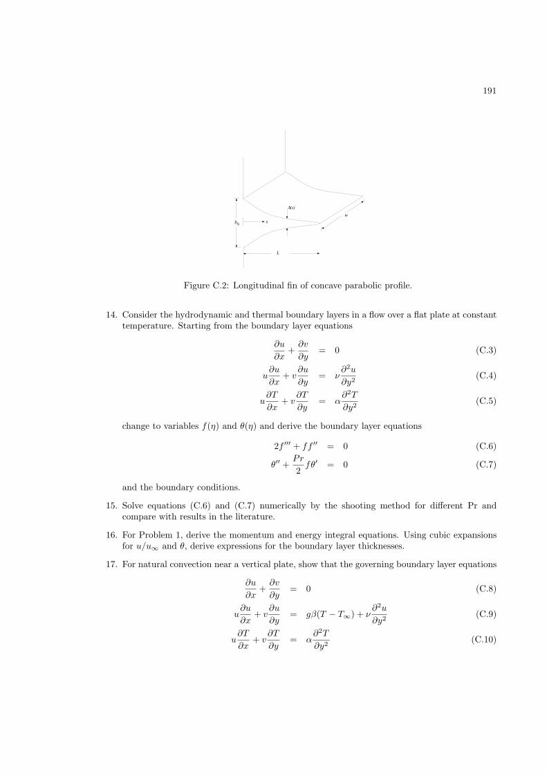
191
δ b x
L
δ(x)
w
Figure C.2: Longitudinal fin of concave parabolic profile.
14. Consider the hydrodynamic and thermal boundary layers in a flow over a flat plate at constanttemperature. Starting from the boundary layer equations
∂u
∂x+∂v
∂y= 0 (C.3)
u∂u
∂x+ v
∂u
∂y= ν
∂2u
∂y2(C.4)
u∂T
∂x+ v
∂T
∂y= α
∂2T
∂y2(C.5)
change to variables f(η) and θ(η) and derive the boundary layer equations
2f ′′′ + ff ′′ = 0 (C.6)
θ′′ +Pr
2fθ′ = 0 (C.7)
and the boundary conditions.
15. Solve equations (C.6) and (C.7) numerically by the shooting method for different Pr andcompare with results in the literature.
16. For Problem 1, derive the momentum and energy integral equations. Using cubic expansionsfor u/u∞ and θ, derive expressions for the boundary layer thicknesses.
17. For natural convection near a vertical plate, show that the governing boundary layer equations
∂u
∂x+∂v
∂y= 0 (C.8)
u∂u
∂x+ v
∂u
∂y= gβ(T − T∞) + ν
∂2u
∂y2(C.9)
u∂T
∂x+ v
∂T
∂y= α
∂2T
∂y2(C.10)
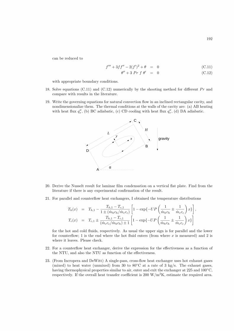
192
can be reduced to
f ′′′ + 3ff ′′ − 2(f ′)2 + θ = 0 (C.11)
θ′′ + 3 Pr f θ′ = 0 (C.12)
with appropriate boundary conditions.
18. Solve equations (C.11) and (C.12) numerically by the shooting method for different Pr andcompare with results in the literature.
19. Write the governing equations for natural convection flow in an inclined rectangular cavity, andnondimensionalize them. The thermal conditions at the walls of the cavity are: (a) AB heatingwith heat flux q′′s , (b) BC adiabatic, (c) CD cooling with heat flux q′′s , (d) DA adiabatic.
gravity
α
LH
A
B
C
D
xy
20. Derive the Nusselt result for laminar film condensation on a vertical flat plate. Find from theliterature if there is any experimental confirmation of the result.
21. For parallel and counterflow heat exchangers, I obtained the temperature distributions
Th(x) = Th,1 −Th,1 − Tc,1
1 ± (mhch/mccc)
[1 − exp−UP
(1
mhch± 1
mccc
)x],
Tc(x) = Tc,1 ±Th,1 − Tc,1
(mccc/mhch) ± 1
[1 − exp−UP
(1
mhch± 1
mccc
)x]
for the hot and cold fluids, respectively. As usual the upper sign is for parallel and the lowerfor counterflow; 1 is the end where the hot fluid enters (from where x is measured) and 2 iswhere it leaves. Please check.
22. For a counterflow heat exchanger, derive the expression for the effectiveness as a function ofthe NTU, and also the NTU as function of the effectiveness.
23. (From Incropera and DeWitt) A single-pass, cross-flow heat exchanger uses hot exhaust gases(mixed) to heat water (unmixed) from 30 to 80C at a rate of 3 kg/s. The exhaust gases,having thermophysical properties similar to air, enter and exit the exchanger at 225 and 100C,respectively. If the overall heat transfer coefficient is 200 W/m2K, estimate the required area.
193
24. (From Incropera and DeWitt) A cross-flow heat exchanger used in cardiopulmonary bypassprocedure cools blood flowing at 5 liters/min from a body temperature of 37C to 25C inorder to induce body hypothermia, which reduces metabolic and oxygen requirements. Thecoolant is ice water at 0C and its flow rate is adjusted to provide an outlet temperature of15C. The heat exchanger operates with both fluids unmixed, and the overall heat transfercoefficient is 750 W/m2K. The density and specific heat of the blood are 1050 kg/m2 and 3740J/kg K, respectively. (a) Determine the heat transfer rate for the exchanger. (b) Calculatethe water flow rate. (c) What is the surface area of the heat exchanger?
25. Show that the energy spectrum for blackbody radiation (Planck’s law)
Eλ =C1
λ5(exp C2
λT − 1)
has a maximum at λ = λm where (Wien’s law)
λmT = 0.1987 C2
Also show that (Stefan-Boltzmann’s law)
∫∞
0
Eλ dλ =C1π
4
15C42
T 4
You can use a symbolic algebra program in this problem.
26. Write a numerical code to evaluate the view factor between two rectangular surfaces (eachof size L × 2L) at 90 with a common edge of length 2L; see Fig. C.3. Compare with theanalytical result.
27. Calculate the view factor again but with a sphere (diameter L/2, center at a distance of L/2from each rectangle, and centered along the length of the rectangles) as an obstacle betweenthe two rectangles; see Fig. C.4.
28. (From Incropera and DeWitt) Consider a diffuse, gray, four-surface enclosure shaped in theform of a tetrahedron (made of four equilateral triangles). The temperatures and emissivitiesof three sides are
T1 = 700K, ǫ1 = 0.7
T2 = 500K, ǫ2 = 0.5
T3 = 300K, ǫ3 = 0.3
The fourth side is well insulated and can be treated as a reradiating surface. Determine itstemperature.
29. An “Aoki” curve is defined as shown in Fig. C.5. Show that when n → ∞, the dimension ofthe curve is D = 1 and the length L→ ∞.
30. Consider conductive rods of thermal conductivity k joined together in the form of a fractaltree (generation n = 3 is shown in Fig. C.6; the fractal is obtained in the limit n → ∞). Thebase and tip temperatures are T0 and T∞, respectively. The length and cross-sectional area of
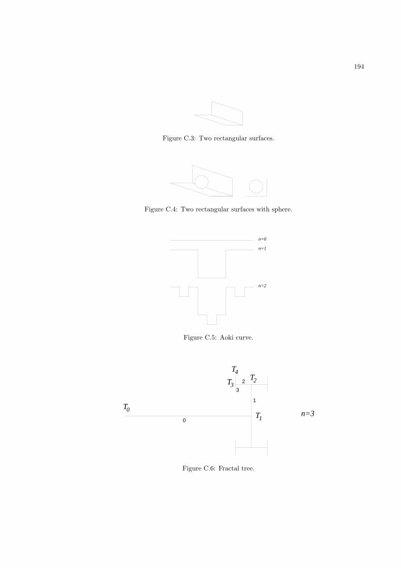
194
Figure C.3: Two rectangular surfaces.
Figure C.4: Two rectangular surfaces with sphere.
n=0
n=1
n=2
Figure C.5: Aoki curve.
n=3T0
T4
T1
T2T3
0
1
2
3
Figure C.6: Fractal tree.
195
bar 0 is L and A, respectively, and those of bar 1 are 2L/β and A/β2, where 1 ≤ β < 2, andso on. Show that the conductive heat transfer through rod 0 is
q =kA
L(T0 − T∞)
(1 − β
2
)
31. The dependence of the rate of chemical reaction on the temperature T is often represented bythe Arrhenius function f(T ) = e−E/T , where E is the activation energy. Writing T ∗ = T/E,show that f(T ∗) has a point of inflexion at T ∗ = 1/2. Plot f(T ∗) in the range T ∗ = 1/16 toT ∗ = 4 as well as its Taylor series approximation to various orders around T ∗ = 1/2. Plot alsothe L2-error in the same range for different orders of the approximation.
32. If e−E/T is proportional to the heat generated within a tank by chemical reaction, and there isheat loss by convection from the tank, show that the temperature of the tank T is determinedby
McdT
dt= ae−E/T − hA(T − T∞)
where M is the mass, c is the specific heat, a is a proportionality constant, h is the convec-tive heat transfer coefficient, A is the convective heat transfer area, and T∞ is the ambienttemperature. Nondimensionalize the equation to
dT ∗
dt∗= e−1/T∗ −H(T ∗ − T ∗
∞)
For T ∗
∞= 0.1, draw the bifurcation diagram with H as the bifurcation parameter, and deter-
mine the bifurcation points.
33. Two bodies at temperatures T1(t) and T2(t), respectively, are in thermal contact with eachother and with the environment. Show that the temperatures are governed by
M1c1dT1
dt+ C(T1 − T2) + C1,∞(T1 − T∞) = Q1
M2c2dT2
dt+ C(T2 − T1) + C2,∞(T2 − T∞) = Q2
where Mi is the mass, ci is the specific heat, the Cs are thermal conductances, and Qi isinternal heat generation. Find the steady state (T 1, T 2) and determine its stability.
34. Using a complete basis, expand the solution of the one-dimensional heat equation
∂T
∂t= α
∂2T
∂x2
with boundary conditions
−k∂T∂x
= q0 at x = 0,
T = T1 at x = L
as an infinite set of ODEs.
196
35. Show that the governing equation of the unsteady, variable-area, convective fin can be writtenin the form
∂T
∂t− ∂
∂x
(a(x)
∂T
∂x
)+ b(x)T = 0
Show that the steady-state temperature distribution with fixed temperatures at the two endsx = 0 and x = L is globally stable.
36. Show numerically that there are two different types of attractors for the following dynamicalsystem.
dx
dt= (λ− λ0)x− y − (x2 + y2)x,
dy
dt= x+ (λ− λ0)y − (x2 + y2)y.
Choose λ0 = 1 and (a) λ = 0.5 and (b) λ = 2.
37. For the two-dimensional, unsteady velocity field ui + vj, where
u = y
v = x− x3 + a cos t
determine the pathline of a fluid particle which is at position (1,1) at time t = 0. Considertwo cases: (a) a = 0, and (b) a = 1. For these two cases find where 11 × 11 points uniformlydistributed within a square of size 0.01 and centered on (1,1) end up. Choose a suitably longfinal time.
38. Find the dimension of the strange attractor for the Lorenz equations
dx
dt= σ(y − x)
dy
dt= λx− y − xz
dz
dt= −bz + xy
where σ = 10, λ = 28 and b = 8/3. Use the method of counting the number of points N(r)within a sphere of radius r from which D = lnN/ ln r.
39. Nondimensionalize and solve the radiative cooling problem
McdT
dt+ σA
(T 4 − T 4
∞
)= 0
with T (0) = Ti.
40. For heat transfer from a heated body with convection and weak radiation, i.e. for
dθ
dτ+ θ + ǫ
(θ + β)
4 − β4
= q
with θ(0) = 1, using symbolic algebra determine the regular perturbation solution up to andincluding terms of order ǫ4. Assuming ǫ = 0.1, β = 1, q = 1, plot the five solutions (with oneterm, with two terms, with three terms, etc.) in the range 0 ≤ τ ≤ 1.
197
41. Consider a body in thermal contact with the environment
McdT
dt+ hA(T − T∞) = 0
where the ambient temperature, T∞(t), varies with time in the form shown below. Find (a)the long-time solution of the system temperature, T (t), and (b) the amplitude of oscillation ofthe system temperature, T (t), for a small period δt.
t
T∞
Tmax
Tmin
δt
Figure C.7: Ambient temperature variation.
42. For a heated body in thermal contact with a constant temperature environment
McdT
dt+ hA(T − T∞) = Q
analyze the conditions for linear stability of PID control.
43. Two heated bodies at temperatures T1(t) and T2(t), respectively, are in thermal contact witheach other and with a constant temperature environment. The temperatures are governed by
M1c1dT1
dt+ C(T1 − T2) + C1,∞(T1 − T∞) = Q1(t)
M2c2dT2
dt+ C(T2 − T1) + C2,∞(T2 − T∞) = Q2(t)
where Q1(t) and Q2(t) are internal heat generations, each one of which can be independentlycontrolled. Using PID control, choose numerical values of the parameters and PID constantsto show numerical results for the different types of responses possible (damped, oscillatory,etc.).
44. Show numerical results for the behavior of two heated bodies in thermal contact with eachother and with a constant temperature environment for on-off control with (a) one thermostat,and (b) two thermostats.
45. Analyze the system controllability of two heated bodies in thermal contact with each other andwith a constant temperature environment for (a) Q1(t) and Q2(t) being the two manipulatedvariables, and (b) with Q1(t) as the only manipulated variable and Q2 constant.
198
46. Run the neural network FORTRAN code in
http://www.nd.edu/ msen/Teaching/IntSyst/Programs/ANN/
for 2 hidden layers with 5 nodes each and 20,000 epochs. Plot the results in the form of exactz vs. predicted z.
47. Consider the heat equation∂T
∂t=∂2T
∂x2
with one boundary condition T (0) = 0. At the other end the temperature, T (1) = u(t) isused as the manipulated variable. Divide the domain into 5 parts and use finite differencesto write the equation as a matrix ODE. Find the controllability matrix and check for systemcontrollability.
48. Determine the semi-derivative and semi-integral of (a) C (a constant), (b) x, and (c) xµ whereµ > −1.
49. Find the time-dependent temperature field for flow in a duct wih constant T∞ and Tin, butwith variable flow rate V (t) = V0 + ∆V sin(ωt) such that V is always positive.
50. Write a computer program to solve the PDE for the previous problem, and compare numericaland analytical results.
51. Derive an expression for heat transfer in a fractal tree-like microchannel net1.
52. Find the steady-state temperature distribution and velocity in a square-loop thermosyphon.The total length of the loop is L and the distribution of the heat rate per unit length is
q(x) =
Q for L/8 ≤ x ≤ L/4,−Q for 5L/8 ≤ x ≤ 3L/4,0 otherwise.
L/4
Q
Q
g
x
1Y. Chen and P. Cheng, Heat transfer and pressure drop in fractal tree-like microchannel nets, International
Journal of Heat and Mass Transfer, Vol. 45, pp. 2643–2648, 2002
199
53. Show that the dynamical system governing the toroidal thermosyphon with known wall tem-perature can be reduced to the Lorenz equations.
54. Draw the steady-state velocity vs. inclination angle diagram for the inclined toroidal ther-mosyphon with mixed heating. Do two cases: (a) without axial condution2, and (b) with axialconduction.
55. Model natural convection in a long, vertical pipe that is being heated from the side at aconstant rate. What is the steady-state fluid velocity in the pipe? Assume one-dimensionalityand that the viscous force is proportional to the velocity.
56. Using the center manifold projection, find the nonlinear behavior of
dx
dt= x2y − x5,
dy
dt= −y + x2,
and hence determine whether the origin is stable.
57. The Brinkman model for the axial flow velocity, u∗(r∗), in a porous cylinder of radius R is
µeff
[d2u∗
dr∗2+
1
r∗du∗
dr∗
]− µ
Ku∗ +G = 0,
where u∗ = 0 at r∗ = R (no-slip at the wall), and ∂u∗/∂r∗ = 0 at r∗ = 0 (symmetry at thecenterline). µeff is the effective viscosity, µ is the fluid viscosity, K is the permeability, and Gis the applied pressure gradient. Show that this can be reduced to the nondimensional form
d2u
dr2+
1
r
du
dr− s2u+
1
M= 0, (C.13)
where M = µeff /µ, Da = K/R2, s2 = (M Da)−1.
58. Using a regular perturbation expansion, show that for s≪ 1, the velocity profile from equation(C.13) is
u =1 − r2
4M
[1 − s2
16
(3 − r2
)]+ . . .
59. Using the WKB method, show that the solution of equation (1) for s≫ 1 is
u = Da
[1 − exp −s(1 − r)√
r
]+ . . .
60. Consider steady state natural convection in a tilted cavity as shown. DA and BC are adiabaticwhile AB and CD have a constant heat flux per unit length. It can be shown that the governingequations in terms of the vorticity ω and the streamfunction ψ are
∂2ψ
∂x2+∂2ψ
∂x2+ ω = 0
∂ψ
∂y
∂ω
∂x− ∂ψ
∂x
∂ω
∂y− Pr
[∂2ω
∂x2+∂2ω
∂y2
]−Ra Pr
[∂T
∂xcosα− ∂T
∂ysinα
]= 0
∂ψ
∂y
∂T
∂x− ∂ψ
∂x
∂T
∂y− ∂2T
∂x2− ∂2T
∂y2= 0
2M. Sen, E. Ramos and C. Trevino, On the steady-state velocity of the inclined toroidal thermosyphon, ASME J.
of Heat Transfer, Vol. 107, pp. 974–977, 1985.
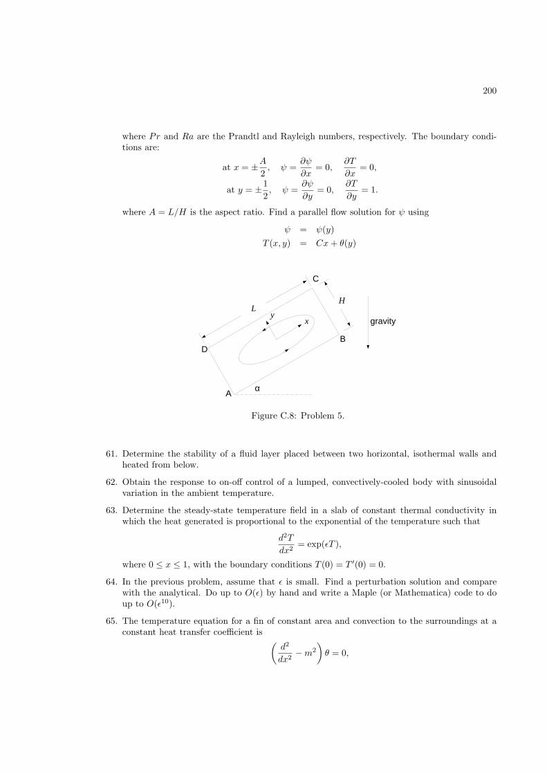
200
where Pr and Ra are the Prandtl and Rayleigh numbers, respectively. The boundary condi-tions are:
at x = ±A2, ψ =
∂ψ
∂x= 0,
∂T
∂x= 0,
at y = ±1
2, ψ =
∂ψ
∂y= 0,
∂T
∂y= 1.
where A = L/H is the aspect ratio. Find a parallel flow solution for ψ using
ψ = ψ(y)
T (x, y) = Cx+ θ(y)
gravity
α
LH
A
B
C
D
xy
Figure C.8: Problem 5.
61. Determine the stability of a fluid layer placed between two horizontal, isothermal walls andheated from below.
62. Obtain the response to on-off control of a lumped, convectively-cooled body with sinusoidalvariation in the ambient temperature.
63. Determine the steady-state temperature field in a slab of constant thermal conductivity inwhich the heat generated is proportional to the exponential of the temperature such that
d2T
dx2= exp(ǫT ),
where 0 ≤ x ≤ 1, with the boundary conditions T (0) = T ′(0) = 0.
64. In the previous problem, assume that ǫ is small. Find a perturbation solution and comparewith the analytical. Do up to O(ǫ) by hand and write a Maple (or Mathematica) code to doup to O(ǫ10).
65. The temperature equation for a fin of constant area and convection to the surroundings at aconstant heat transfer coefficient is
(d2
dx2−m2
)θ = 0,
201
where θ = T − T∞. Determine the eigenfunctions of the differential operator for each combi-nation of Dirichlet and Neumann boundary conditions at the two ends x = 0 and x = L.
66. Add radiation to a convective fin with constant area and solve for small radiative effects withboundary conditions corresponding to a known base temperature and adiabatic tip.
67. Find the temperature distribution in a slightly tapered 2-dimensional convective fin with knownbase temperature and adiabatic tip.
x
68. Prove Hottel’s crossed string method to find the view factor FAB between two-dimensionalsurfaces A and B with some obstacles between them as shown. The dotted lines are tightlystretched strings. The steps are:
(a) Assuming the strings to be imaginary surfaces, apply the summation rule to each one ofthe sides of figure abc.
(b) Manipulating these equations and applying reciprocity, show that
Fab−ac =Aab +Aac −Abc
2Aab.
(c) For abd find Fab−bd in a similar way.
(d) Use the summation rule to show that
Fab−cd =Abc +Aad −Aac −Abd
2Aab
(e) Show that Fab−cd = AAFAB/Aab.
(f) Show the final result
FA−B =Abc +Aad −Aac −Abd
2AA
69. Complete the details to derive the Nusselt result for laminar film condensation on a verticalflat plate. Find from the literature if there is any experimental confirmation of the result.
70. Consider the hydrodynamic and thermal boundary layers in a flow over a flat plate at constanttemperature. Use a similarity transformation on the boundary layer equations to get
2f ′′′ + ff ′′ = 0,
θ′′ +Pr
2fθ′ = 0.
Using the shooting method and the appropriate boundary conditions, solve the equations fordifferent Pr and compare with the results in the literature.
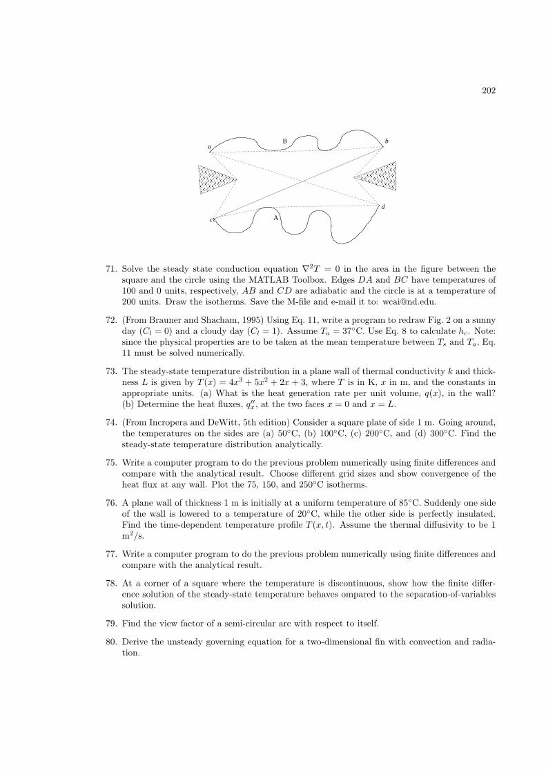
202
b
d
aB
Acc
71. Solve the steady state conduction equation ∇2T = 0 in the area in the figure between thesquare and the circle using the MATLAB Toolbox. Edges DA and BC have temperatures of100 and 0 units, respectively, AB and CD are adiabatic and the circle is at a temperature of200 units. Draw the isotherms. Save the M-file and e-mail it to: [email protected].
72. (From Brauner and Shacham, 1995) Using Eq. 11, write a program to redraw Fig. 2 on a sunnyday (Cl = 0) and a cloudy day (Cl = 1). Assume Ta = 37C. Use Eq. 8 to calculate hc. Note:since the physical properties are to be taken at the mean temperature between Ts and Ta, Eq.11 must be solved numerically.
73. The steady-state temperature distribution in a plane wall of thermal conductivity k and thick-ness L is given by T (x) = 4x3 + 5x2 + 2x + 3, where T is in K, x in m, and the constants inappropriate units. (a) What is the heat generation rate per unit volume, q(x), in the wall?(b) Determine the heat fluxes, q′′x , at the two faces x = 0 and x = L.
74. (From Incropera and DeWitt, 5th edition) Consider a square plate of side 1 m. Going around,the temperatures on the sides are (a) 50C, (b) 100C, (c) 200C, and (d) 300C. Find thesteady-state temperature distribution analytically.
75. Write a computer program to do the previous problem numerically using finite differences andcompare with the analytical result. Choose different grid sizes and show convergence of theheat flux at any wall. Plot the 75, 150, and 250C isotherms.
76. A plane wall of thickness 1 m is initially at a uniform temperature of 85C. Suddenly one sideof the wall is lowered to a temperature of 20C, while the other side is perfectly insulated.Find the time-dependent temperature profile T (x, t). Assume the thermal diffusivity to be 1m2/s.
77. Write a computer program to do the previous problem numerically using finite differences andcompare with the analytical result.
78. At a corner of a square where the temperature is discontinuous, show how the finite differ-ence solution of the steady-state temperature behaves ompared to the separation-of-variablessolution.
79. Find the view factor of a semi-circular arc with respect to itself.
80. Derive the unsteady governing equation for a two-dimensional fin with convection and radia-tion.
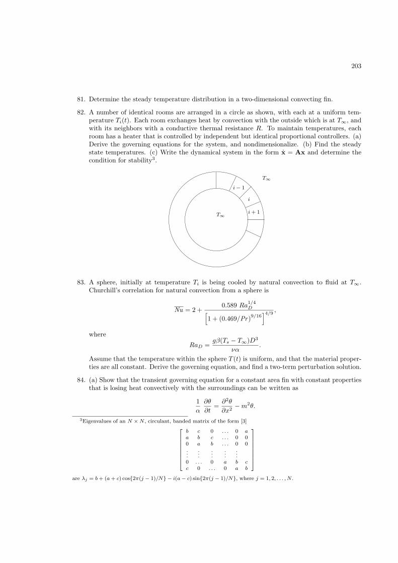
203
81. Determine the steady temperature distribution in a two-dimensional convecting fin.
82. A number of identical rooms are arranged in a circle as shown, with each at a uniform tem-perature Ti(t). Each room exchanges heat by convection with the outside which is at T∞, andwith its neighbors with a conductive thermal resistance R. To maintain temperatures, eachroom has a heater that is controlled by independent but identical proportional controllers. (a)Derive the governing equations for the system, and nondimensionalize. (b) Find the steadystate temperatures. (c) Write the dynamical system in the form x = Ax and determine thecondition for stability3.
i − 1
i
i + 1
T∞
T∞
83. A sphere, initially at temperature Ti is being cooled by natural convection to fluid at T∞.Churchill’s correlation for natural convection from a sphere is
Nu = 2 +0.589 Ra
1/4D[
1 + (0.469/Pr)9/16
]4/9,
where
RaD =gβ(Ts − T∞)D3
να.
Assume that the temperature within the sphere T (t) is uniform, and that the material proper-ties are all constant. Derive the governing equation, and find a two-term perturbation solution.
84. (a) Show that the transient governing equation for a constant area fin with constant propertiesthat is losing heat convectively with the surroundings can be written as
1
α
∂θ
∂t=∂2θ
∂x2−m2θ.
3Eigenvalues of an N × N , circulant, banded matrix of the form [3]
2
6
6
6
6
6
6
6
4
b c 0 . . . 0 aa b c . . . 0 00 a b . . . 0 0...
.
.....
.
.....
0 . . . 0 a b cc 0 . . . 0 a b
3
7
7
7
7
7
7
7
5
are λj = b + (a + c) cos2π(j − 1)/N − i(a − c) sin2π(j − 1)/N, where j = 1, 2, . . . , N .
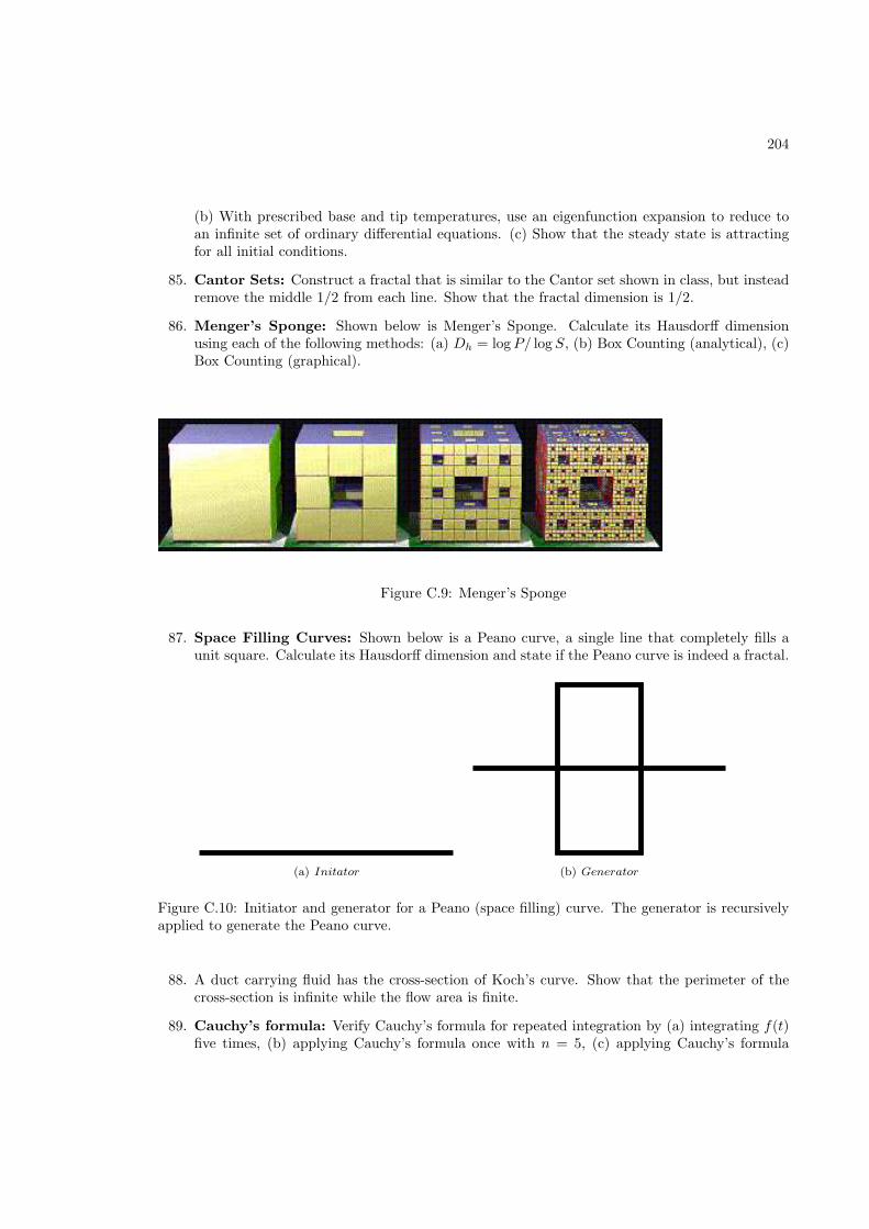
204
(b) With prescribed base and tip temperatures, use an eigenfunction expansion to reduce toan infinite set of ordinary differential equations. (c) Show that the steady state is attractingfor all initial conditions.
85. Cantor Sets: Construct a fractal that is similar to the Cantor set shown in class, but insteadremove the middle 1/2 from each line. Show that the fractal dimension is 1/2.
86. Menger’s Sponge: Shown below is Menger’s Sponge. Calculate its Hausdorff dimensionusing each of the following methods: (a) Dh = logP/ logS, (b) Box Counting (analytical), (c)Box Counting (graphical).
Figure C.9: Menger’s Sponge
87. Space Filling Curves: Shown below is a Peano curve, a single line that completely fills aunit square. Calculate its Hausdorff dimension and state if the Peano curve is indeed a fractal.
(a) Initator (b) Generator
Figure C.10: Initiator and generator for a Peano (space filling) curve. The generator is recursivelyapplied to generate the Peano curve.
88. A duct carrying fluid has the cross-section of Koch’s curve. Show that the perimeter of thecross-section is infinite while the flow area is finite.
89. Cauchy’s formula: Verify Cauchy’s formula for repeated integration by (a) integrating f(t)five times, (b) applying Cauchy’s formula once with n = 5, (c) applying Cauchy’s formula
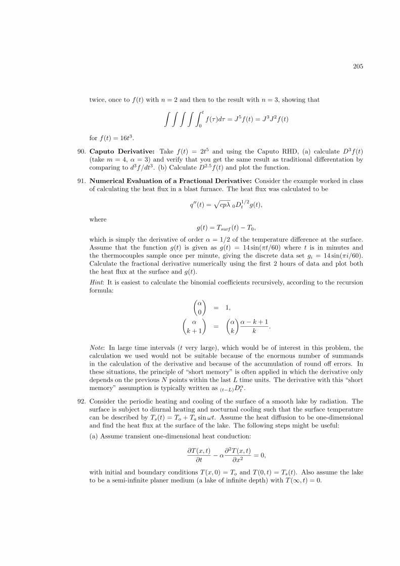
205
twice, once to f(t) with n = 2 and then to the result with n = 3, showing that
∫ ∫ ∫ ∫ ∫ t
0
f(τ)dτ = J5f(t) = J3J2f(t)
for f(t) = 16t3.
90. Caputo Derivative: Take f(t) = 2t5 and using the Caputo RHD, (a) calculate D3f(t)(take m = 4, α = 3) and verify that you get the same result as traditional differentation bycomparing to d3f/dt3. (b) Calculate D2.5f(t) and plot the function.
91. Numerical Evaluation of a Fractional Derivative: Consider the example worked in classof calculating the heat flux in a blast furnace. The heat flux was calculated to be
q′′(t) =√cpλ 0D
1/2t g(t),
whereg(t) = Tsurf (t) − T0,
which is simply the derivative of order α = 1/2 of the temperature difference at the surface.Assume that the function g(t) is given as g(t) = 14 sin(πt/60) where t is in minutes andthe thermocouples sample once per minute, giving the discrete data set gi = 14 sin(πi/60).Calculate the fractional derivative numerically using the first 2 hours of data and plot boththe heat flux at the surface and g(t).
Hint: It is easiest to calculate the binomial coefficients recursively, according to the recursionformula:
(α
0
)= 1,
(α
k + 1
)=
(α
k
)α− k + 1
k.
Note: In large time intervals (t very large), which would be of interest in this problem, thecalculation we used would not be suitable because of the enormous number of summandsin the calculation of the derivative and because of the accumulation of round off errors. Inthese situations, the principle of “short memory” is often applied in which the derivative onlydepends on the previous N points within the last L time units. The derivative with this “shortmemory” assumption is typically written as (t−L)D
αt .
92. Consider the periodic heating and cooling of the surface of a smooth lake by radiation. Thesurface is subject to diurnal heating and nocturnal cooling such that the surface temperaturecan be described by Ts(t) = To + Ta sinωt. Assume the heat diffusion to be one-dimensionaland find the heat flux at the surface of the lake. The following steps might be useful:
(a) Assume transient one-dimensional heat conduction:
∂T (x, t)
∂t− α
∂2T (x, t)
∂x2= 0,
with initial and boundary conditions T (x, 0) = To and T (0, t) = Ts(t). Also assume the laketo be a semi-infinite planer medium (a lake of infinite depth) with T (∞, t) = 0.
206
(b) Non-dimensionalize the problem with a change of variables ξ = α−1/2x and θ(x, t) =T (x, t) − To.
(c) Use the following Laplace transform properties to transform the problem into the Laplacedomain:
L[∂αf(x, t)
∂tα]
= sαF (x, s) (with 0 initial conditions)
and
L[∂αf(x, t)
∂xα
]=
∂α
∂xαF (x, s)
(d) Solve the resulting second order differential equation for Θ(ξ, s) by applying the trans-formed boundary conditions.
(e) Find ∂Θ/∂ξ and then substitute Θ(ξ, s) into the result. Now take the inverse Laplacetransform of ∂Θ/∂ξ and convert back to the original variables. Be careful! The derivative oforder 1/2 of a constant is not zero! (see simplifications in (g) to simplify)
(f) You should now have an expression for ∂T (x, t)/∂x. Substitute this into Fourier’s Law tocalculate the heat flux, q′′(x, t) = −k ∂T (x, t)/∂x.
(g) Evaluate this expression at the surface (x = 0) to find the heat flux at the surface of thelake. The following simplifications might be helpful:
∂1/2C
∂t1/2=
C
πt1/2
∂α[Cg(t)]
∂tα= C
∂αg(t)
∂tα
(h) The solution should look now look like
q′′s (t) =k
α1/2
d1/2(Ta sinωt)
dt1/2
93. Describe how you would solve this problem using more typical methods and what other infor-mation would be required.
94. Consider radiation between two long concentric cylinders of diameters D1 (inner) and D2
(outer). (a) What is the view factor F12. (b) Find F22 and F21 in terms of the cylinderdiameters.
95. Temperatures at the two sides of a plane wall shown in Fig. C.11 are TL and TR, respectively.For small ǫ, find a perturbation steady-state temperature distribution T (x) if the dependenceof thermal conductivity on the temperature has the form
k(T ) = k0
(1 +
T − TL
TR − TLǫ
).
96. One side of a plane wall shown in Fig. C.12 has a fixed temperature and the other is adiabatic.With an initial condition T (x, 0) = f(x), determine the temperature distribution in the wallT (x, t) at any other time. Assume constant properties.
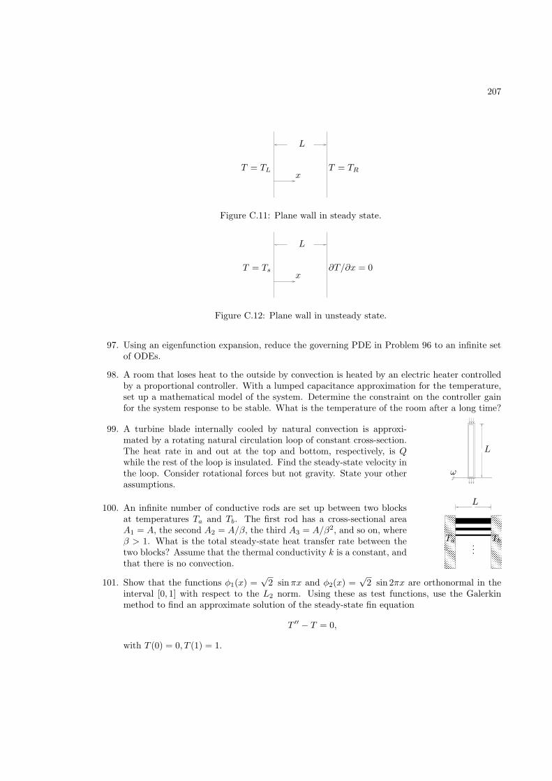
207
L
T = TL T = TRx
Figure C.11: Plane wall in steady state.
L
T = Ts ∂T/∂x = 0x
Figure C.12: Plane wall in unsteady state.
97. Using an eigenfunction expansion, reduce the governing PDE in Problem 96 to an infinite setof ODEs.
98. A room that loses heat to the outside by convection is heated by an electric heater controlledby a proportional controller. With a lumped capacitance approximation for the temperature,set up a mathematical model of the system. Determine the constraint on the controller gainfor the system response to be stable. What is the temperature of the room after a long time?
99. A turbine blade internally cooled by natural convection is approxi-mated by a rotating natural circulation loop of constant cross-section.The heat rate in and out at the top and bottom, respectively, is Qwhile the rest of the loop is insulated. Find the steady-state velocity inthe loop. Consider rotational forces but not gravity. State your otherassumptions.
L
ω
100. An infinite number of conductive rods are set up between two blocksat temperatures Ta and Tb. The first rod has a cross-sectional areaA1 = A, the second A2 = A/β, the third A3 = A/β2, and so on, whereβ > 1. What is the total steady-state heat transfer rate between thetwo blocks? Assume that the thermal conductivity k is a constant, andthat there is no convection.
L
Ta Tb...
101. Show that the functions φ1(x) =√
2 sinπx and φ2(x) =√
2 sin 2πx are orthonormal in theinterval [0, 1] with respect to the L2 norm. Using these as test functions, use the Galerkinmethod to find an approximate solution of the steady-state fin equation
T ′′ − T = 0,
with T (0) = 0, T (1) = 1.
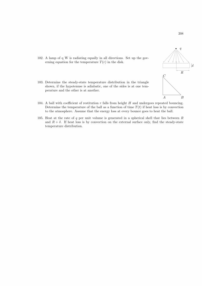
208
102. A lamp of q W is radiating equally in all directions. Set up the gov-erning equation for the temperature T (r) in the disk.
q
d
R
103. Determine the steady-state temperature distribution in the triangleshown, if the hypotenuse is adiabatic, one of the sides is at one tem-perature and the other is at another.
A B
C
104. A ball with coefficient of restitution r falls from height H and undergoes repeated bouncing.Determine the temperature of the ball as a function of time T (t) if heat loss is by convectionto the atmosphere. Assume that the energy loss at every bounce goes to heat the ball.
105. Heat at the rate of q per unit volume is generated in a spherical shell that lies between Rand R + δ. If heat loss is by convection on the external surface only, find the steady-statetemperature distribution.
References
[1] R. Acosta, M. Sen, and E. Ramos. Single-phase natural circulation in a tilted square loop.Warme- und Stoffubertragung, 21(5):269–275, 1987.
[2] N.U. Ahmed. Semigroup Theory with Applications to Systems and Control. Longman, Harlow,U.K., 1991.
[3] R. Aldrovandi. Special Matrices of Mathematical Physics: Stochastic, Circulant and BellMetrices. World Scientific, Singapore, 2001.
[4] S. Alotaibi. Temperature Controllability in Cross-Flow Heat Exchangers and Long Ducts. PhDthesis, Department of Aerospace and Mechanical Engineering, University of Notre Dame, NotreDame, IN, 2003.
[5] S. Alotaibi, W.J. Goodwine M. Sen, and K.T. Yang. Controllability of cross-flow heat ex-changers. International Journal of Heat and Mass Transfer, 47:913–924, 2004.
[6] S. Alotaibi, M. Sen, J.W. Goodwine, and K.T. Yang. Numerical simulation of the thermalcontrol of heat exchangers. Numerical Heat Transfer A, 41:229–244, 2002.
[7] S. Alotaibi, M. Sen, W.J. Goodwine, and K.T. Yang. Flow-based control of temperature inlong ducts. International Journal of Heat and Mass Transfer, 47:4995–5009, 2004.
[8] K.A. Antonopoulos and C. Tzivanidis. A correlation for the thermal delay of building. Re-newable Energy, 6(7):687–699, 1995.
[9] P.J. Antsaklis and A.N. Michel. Linear Systems. McGraw-Hill, New York, 1997.
[10] R. Arena, R. Caponetto, L. Fortuna, and D. Porto. Nonlinear Noninteger Order Circuits andSystems–An Introduction. World Scientific, Singapore, 2000.
[11] Arpaci and Larson. Convection Heat Transfer. Prentice-Hall, 1984.
[12] V.S. Arpaci, S.-H. Kao, and A. Selamet. Introduction to Heat Transfer. Prentice-Hall, UpperSaddle River, NJ, 1999.
[13] A. Aziz and T.Y. Na. Perturbation Methods in Heat Transfer. Hemisphere Publ. Corp.,Washington, DC, 1984.
[14] H.D. Baehr and K. Stephan. Heat and Mass Transfer. Springer, New York, 1998.
[15] A.-L. Barabasi. Linked: The New Science of Networks. Perseus, Cambridge, MA, 2002.
209
REFERENCES 210
[16] C Baruch and S. Darrell. On stability of systems of delay differential equations. J. Comp.Appl. Math., 117:137–158, 2000.
[17] J.L. Battaglia, L. Le Lay, J.C. Batsale, A. Oustaloup, and O. Cois. Heat flux estimationthrough inverted non-integer identification models. International Journal of Thermal Sciences,39(3):374–389, 2000.
[18] H.H. Bau. Control of Marangoni-Benard convection. International Journal of Heat and MassTransfer, 42(7):1327–1341, 1999.
[19] Y. Bayazitoglu and M.N. Ozisik. Elements of Heat Transfer. McGraw-Hill, New York, 1988.
[20] M. Becker. Heat Transfer, A Modern Approach. Plenum Press, New York, 1986.
[21] A. Bejan. Convection Heat Transfer. John Wiley, New York, 1984.
[22] A. Bejan. Heat Transfer. John Wiley, New York, 1993.
[23] R. Bellman and K.L. Cooke. Differential-Difference Equations. Academic Press, New York,1963.
[24] C.O. Bennett. Momentum, Heat, and Mass Transfer. McGraw-Hill, New York, 3rd edition,1982.
[25] M.Q. Brewster. Thermal Radiative Transfer and Properties. John Wiley, New York, 3rdedition, 1992.
[26] L.C. Burmeister. Heat Transfer. Dover, New York, 1982.
[27] L.C. Burmeister. Convection Heat Transfer. John Wiley, New York, 2nd edition, 1993.
[28] E.F. Camacho and C. Bordons. Model Predictive Control in the Process Industry. Springer,London, 2001.
[29] V.P. Carey. Liquid-Vapor Phase-Change Phenomena. Hemisphere Publ. Corp., Washington,DC, 1992.
[30] J. Carr. Applications of Centre Manifold Theory. Springer-Verlag, New York, 1981.
[31] H.S. Carslaw and J.C. Jaeger. Conduction of Heat in Solids. Clarendon Press, Oxford, UK,1959.
[32] O. Castillo and P. Melin. Soft Computing for Control of Non-Linear Dynamical Systems.Physica-Verlag, Heidelberg, 2001.
[33] Cebeci and Bradshaw. Physical and Computational Aspects of Convective Heat Transfer.Springer-Verlag, 1984.
[34] A.J. Chapman. Fundamentals of Heat Transfer. Macmillan, New York, 1987.
[35] C.K. Charny. Mathematical models of bioheat transfer. In Y.I. Cho, editor, Advances in HeatTransfer, volume 22, pages 19–155. Academic Press, New York, 1992.
[36] G. Chen. Heat transfer in micro- and nanoscale photonic devices. In C.-L. Tien, editor, AnnualReview of Heat Transfer, volume 7, chapter 1. Begell House, New York, 1996.
REFERENCES 211
[37] G. Chen and G. Chen. Linear Stochastic Control Systems. CRC Press, Boca Raton, 1995.
[38] P.D. Christofides. Nonlinear and Robust Control of PDE Systems. Birkhauser, Boston, 2002.
[39] P.D. Christofides and Dautidis P. Feed-back control of hyperbolic PDE systems. AIChEJournal, 412:3063, 1978.
[40] J. Chu. Application of a discrete optimal tracking controller to an industrial electrical heaterwith pure delay. J. Proc. Cont., 5(1):3–8, 1995.
[41] J. Chu, Su H., and x. Hu. A time-delay control algorithm for an industrial electrical heater.J. Proc. Cont., 3(4):220–224, 1993.
[42] Collier. Convective Boiling and Condensation. McGraw-Hill, 1984.
[43] C. Comstock. On the delayed hot water problem. Heat and Mass Transfer, 96:166–171, 1974.
[44] J. Crank. Free and Moving Boundary Problems. Clarendon Press, Oxford, U.K., 1984.
[45] L. Dai. Singular Control Systems. Springer-Verlag, Berlin, 1989.
[46] D. Dıaz, M. Sen, and K.T. Yang. Effect of delay in thermal systems with long ducts. To bepublished in International Journal of Thermal Sciences, 2004.
[47] G. Dıaz. Simulation and Control of Heat Exchangers using Artificial Neural Networks. PhDthesis, Department of Aerospace and Mechanical Engineering, University of Notre Dame, NotreDame, IN, 2000.
[48] G. Dıaz, K.T. Yang M. Sen, and R.L. McClain. Simulation of heat exchanger performance byartificial neural networks. International Journal of HVAC&R Research, 5(3):195–208, 1999.
[49] G. Dıaz, M. Sen, K.T. Yang, and R.L. McClain. Adaptive neurocontrol of heat exchangers.ASME Journal of Heat Transfer, 123(3):417–612, 2001.
[50] G. Dıaz, M. Sen, K.T. Yang, and R.L. McClain. Dynamic prediction and control of heatexchangers using artificial neural networks. International Journal of Heat and Mass Transfer,44(9):1671–1679, 2001.
[51] G. Dıaz, M. Sen, K.T. Yang, and R.L. McClain. Stabilization of a neural network-basedtemperature controller for heat exchangers. Proceedings of the 12th International Heat TransferConference, 4:225–230, 2002.
[52] G. Dıaz, M. Sen, K.T. Yang, and R.L. McClain. Stabilization of thermal neurocontrollers. Tobe published in Applied Artificial Intelligence, 2004.
[53] K.R. Diller. Models of bioheat transfer processes at high and low temperatures. In Y.I. Cho,editor, Advances in Heat Transfer, volume 22, pages 157–357. Academic Press, New York,1992.
[54] C. Doumanidis and N. Fourligkas. Distributed-parameter control of the heat source trajectoryin thermal materials processing. ASME Journal of Manufacturing Science and Engineering,118(4):571–578, 1996.
REFERENCES 212
[55] C. Doumanidis and N. Fourligkas. Distributed-parameter control of the heat source trajectoryin thermal materials processing. ASME Journal of Manufacturing Science and Engineering,118(4):571–578, 1996.
[56] P.G. Drazin. Nonlinear Systems. Cambridge University Press, Cambridge, U.K., 1992.
[57] R.D. Driver. Ordinary and Delay Differential Equations. Springer-Verlag, New York, 1977.
[58] D.K. Edwards. Radiation Heat Transfer Notes. Hemisphere Pub. Corp., Washington, DC, 3rdedition, 1981.
[59] P. Elgar. Sensors for Measurement and Control. Longman, Essex, U.K., 1998.
[60] J. Feder. Fractals. Plenum, New York, 1988.
[61] W. Franco. Hydrodynamics and Control in Thermal-Fluid Networks. PhD thesis, Departmentof Aerospace and Mechanical Engineering, University of Notre Dame, Notre Dame, IN, 2003.
[62] W. Franco, M. Sen, K.T. Yang, and R.L. McClain. Comparison of thermal-hydraulic networkcontrol strategies. Proceedings of the Institution of Mechanical Engineers, Part I: Journal ofSystems and Control Engineering, 217:35–47, 2003.
[63] W. Franco, M. Sen, K.T. Yang, and R.L. McClain. Dynamics of thermal-hydraulic networkcontrol strategies. Experimental Heat Transfer, 17(3):161–179, 2004.
[64] M. Gad-el-Hak. Flow Control: Passive, Active and Reactive Flow Management. CambridgeUniversity Press, Cambridge, U.K., 2000.
[65] V. Ganapathy. Applied Heat Transfer. PennWell Pub. Co., Tulsa, OK, 1982.
[66] B. Gebhart. Heat Conduction and Mass Diffusion. McGraw-Hill, New York, 1993.
[67] B. Gebhart, Y. Jaluria, R.L. Mahajan, and B. Sammakia. Buoyancy-Induced Flows and Trans-port. Hemisphere Publ. Corp., New York, 1988.
[68] U. Grigull. Heat Conduction. Hemisphere Pub. Corp., Washington, D.C., 1984.
[69] J. S. Guillermo, D. Aniruddha, and S.P. Bhattacharyya. PI stabilization of first-order systemswith time delay. Automatica, 37:2020–2031, 2001.
[70] L. Hach and Y. Katoh. Thermal responses in control loop in indirect control of indoor en-vironment of non-air-conditioned space with quasi-steady-state model. JSME InternationalJournal Series C-Mechanical Systems Machine Elements And Manufacturing, 46(1):197–211,2003.
[71] J.K. Hale and S.M. Lunel. Introduction to Functional Differential Equations. Springer-Verlag,New York, 1993.
[72] E.G. Hansen. Hydronic System Design and Operation. McGraw-Hill, New York, 1985.
[73] S. Haykin. Neural Networks: A Comprehensive Foundation. Macmillan, New York, 1999.
[74] G. Henryk, G. Piotr, and K. Adam. Analysis and Synthesis of Time Delay Systems. JohnWiley Sons, Chichester, 1989.
REFERENCES 213
[75] M.A. Henson and D.E. Seborg, editors. Nonlinear Process Control. Prentice Hall, UpperSaddle River, NJ, 1997.
[76] G.F. Hewitt. Process Heat Transfer. CRC Press, Boca Raton, 1994.
[77] J.M. Hill and J.N. Dewynne. Heat Conduction. Blackwell Scientific Publications, Oxford,U.K., 1987.
[78] E.J. Hinch. Perturbation Methods. Cambridge University Press, Cambridge, U.K., 1991.
[79] K.-H. Hoffman and W. Krabs. Optimal Control of Partial Differential Equations. Springer-Verlag, Berlin, 1991.
[80] J.P. Holman. Heat Transfer. McGraw-Hill, New York, 7th edition, 1990.
[81] M.H. Holmes. Laminar flow forced convection in ducts, a source book for compact heat ex-changer analytical data. Springer-Verlag, New York, 1995.
[82] M.F. Hordeski. HVAC Control in the New Millennium. Fairmont Press, Liburn, GA, 2001.
[83] L.E. Howle. Control of Rayleigh-Benard convection in a small aspect ratio container. Inter-national Journal of Heat and Mass Transfer, 40(4):817–822, 1997.
[84] C.J. Huang, C.C. Yu, and S.H. Shen. Selection of measurement locations for the control ofrapid thermal processor. Automatica, 36(5):705–715, 2000.
[85] G. Huang, L. Nie, Y. Zhao, W. Yang, Q. Wu, and L. Liu. Temperature control system of heatexchangers, an application of DPS theory. Lecture Notes in Control Information Sciences,159:68–76, 1991.
[86] H. Ibach and H. Luth. Solid-State Physics. Springer, New York, 1990.
[87] D. Ibrahim. Microcontroller-Based Temperature Monitoring and Control. Newnes, Oxford,2002.
[88] F.P. Incropera and D.P. Dewitt. Fundamentals of Heat and Mass Transfer. John Wiley, NewYork, 5th edition, 2002.
[89] L. Irena and R. Triggiani. Deterministic Control Theory for Infinite Dimensional Systems,Vols. I and II Encyclopedia of Mathematics. Cambridge University Press, 1999.
[90] V.P. Isachenko, V.A. Osipova, and A.S. Sukomel. Heat Transfer. Mir, Moscow, 1977.
[91] A. Isidori. Nonlinear Control Systems. Springer, London, 1995.
[92] A. Ito, H. Kanoh, and M. Masubuchi. MWR approximation and modal control of parallel andcounterflow heat exchangers. Proc, 2nd IFAC Symposium on Distributed-Parameter Systems,41, 1978.
[93] O.L.R. Jacobs. Introduction to Control Theory. 2nd Ed., Oxford University Press, Oxford,1993.
[94] M. Jakob. Heat Transfer, volume II. John Wiley, New York, 1957.
[95] Y. Jaluria. Natural Convection Heat and Mass Transfer. Pergamon Press, New York, 1980.
REFERENCES 214
[96] Y. Jaluria. Computational Heat Transfer. Washington, DC, 1986.
[97] Y. Jaluria and K.E. Torrance. Computational Heat Transfer. Taylor and Francis, New York,2nd edition, 2003.
[98] S. Kakac. Convective Heat Transfer. CRC Press, Boca Raton, 2nd edition, 1995.
[99] S. Kakac, R.K. Shah, and W. Aung, editors. Handbook of Single-Phase Convective HeatTransfer. John Wiley, New York, 1983.
[100] S. Kakac and Y. Yener. Heat Conduction. Taylor and Francis, Washington, DC, 3rd edition,1993.
[101] R.D. Karam. Satellite Thermal Control for Systems Engineers. AIAA, Reston, VA, 1998.
[102] M. Kaviany. Principles of Convective Heat Transfer. Springer-Verlag, New York, 1994.
[103] M. Kaviany. Principles of Heat transfer in Porous Media. Springer-Verlag, New York, 2ndedition, 1995.
[104] W.M. Kays and M.E. Crawford. Convective Heat and Mass Transfer. McGraw-Hill, New York,3rd edition, 1993.
[105] W.M. Kays and A.L. London. Compact Heat Exchangers. McGraw-Hill, San Francisco, 3rdedition, 1984.
[106] D.Q. Kern. Process Heat Transfer. McGraw-Hill International, Auckland, 1950.
[107] J. Kevorkian and J.D. Cole. Multiple Scale and Singular Perturbation Methods. Springer, NewYork, 1996.
[108] M.-H. Kim, S.Y. Lee, S.S. Mehendale, and R.L. Webb. Microscale heat exchanger design forevaporator and condenser applications. In J.P. Hartnett, T.F. Irvine, Y.I. Cho, and G.A.Greene, editors, Advances in Heat Transfer, volume 37, pages 297–429. Academic Press, Am-sterdam, 2003.
[109] C. Kittel and H. Kroemer. Thermal Physics. W.H. Freeman & Co., San Francisco, 2nd edition,1980.
[110] J. Klamka. Controllability of Dynamical Systems. Kluwer, Dordrecht, Netherlands, 1991.
[111] F. Kreith and W.Z. Black. Basic Heat Transfer. Harper and Row, Cambridge, U.K., 1980.
[112] F. Kreith and M.S. Bohn. Principles of Heat Transfer. West Publ. Co., St. Paul, MN, 5thedition, 1993.
[113] A. Kumar and P. Daoutidis. Control of Nonlinear Differential Algebraic Equation Systems.Chapman and Hall/CRC, Boca Raton, FL, 1999.
[114] J.R. Leigh. Temperature Measurement and Control. Peregrinus, London, 1987.
[115] J.I. Levenhagen and D.H. Spethmann. HVAC Controls and Systems. Mc-Graw-Hill, NewYork, 1993.
[116] W.S. Levine, editor. Control System Fundamentals. CRC Press, Boca Raton, FL, 2000.
REFERENCES 215
[117] J.H. Lienhard. A Heat Transfer Textbook. Prentice-Hall, Englewood Cliffs, NJ, 1981.
[118] J.L. Lions. On the controllability of distributed systems. Natl. Acad. Sci. USA, 94:4828–4835,1997.
[119] W.W. Liou and Y. Fang. Microfluid Mechanics: Principles and Modeling. McGraw Hill, NewYork, 2006.
[120] B. Liu and T.R. Marchant. The occurrence of limit-cycles during feedback control of microwaveheating. Mathematical and Computer Modelling, 35(9-10):1095–1118, 2002.
[121] L. Ljung. System Identification: Theory for the User. Prentice-Hall, Upper Saddle River, N.J.,second edition, 1999.
[122] A. Luikov. Heat and Mass Transfer. Mir, Moscow, 1980.
[123] A. Majumdar. Microscale energy transport in solids. In C.-L. Tien, A. Majumdar, and F.M.Gerner, editors, Microscale Energy Transport, chapter 1. Taylor and Francis, Washington, DC,1998.
[124] A. Majumdar. Microscale transport phenomena. In W.M. Rohsenow, J.P Hartnett, and Y.I.Cho, editors, Handbook of Heat Transfer, chapter 8. McGraw-Hill, New York, 1998.
[125] T. Marimbordes, A.O. El Moctar, and H. Peerhossaini. Active control of natural convection ina fluid layer with volume heat dissipation. International Journal of Heat and Mass Transfer,45(3):667–678, 2002.
[126] W.J. Minkowycz, E.M. Sparrow, G.E. Schneider, and R.H. Pletcher, editors. Handbook ofNumerical Heat Transfer. John Wiley, New York, 1988.
[127] M. Modest. Radiative Heat Transfer. Academic Press, Amsterdam, 2003.
[128] W. Munk. The delayed hot-water problem, brief notes. ASME J. Applied Mechanics, 21(10):?–?, 1954.
[129] O. Nelles. Nonlinear System Identification. Springer, Berlin, 2001.
[130] D.A. Nield and A. Bejan. Convection in Porous Media. Springer-Verlag, New York, 2ndedition, 1999.
[131] M. Nørgaard, O. Ravn, N.K. Poulsen, and L.K. Hansen. Neural Networks for Modelling andControl of Dynamic Systems. Springer, London, 2000.
[132] K. Ogata. Modern Control Engineering. Prentice-Hall, Englewood Cliffs, N.J., second edition,1990.
[133] P.H. Oosthuizen and D. Naylor. Introduction to Convective Heat Transfer Analysis. McGraw-Hill, New York, 3rd edition, 1998.
[134] A. Oustaloup. Systemes Asservis Lineaires d’Ordre Fractionnaire: Theorie et Practique. Mas-son, Paris, 1983.
[135] A. Oustaloup. La Derivation Non Entiere. Hermes, Paris, 1995.
REFERENCES 216
[136] M.N. Ozisik. Boundary Value Problems of Heat Conduction. Dover Publications, New York,1968.
[137] M.N. Ozisik. Heat Conduction. John Wiley, New York, 1980.
[138] M.N. Ozisik. Heat Transfer, A Basic Approach. McGraw-Hill, New York, 1985.
[139] A. Pacheco-Vega. Simulation of Compact Heat Exchangers using Global Regression and SoftComputing. PhD thesis, Department of Aerospace and Mechanical Engineering, University ofNotre Dame, Notre Dame, IN, 2002.
[140] A. Pacheco-Vega, G. Dıaz, M. Sen, K.T. Yang, and R.L. McClain. Heat rate predictions inhumid air-water heat exchangers using correlations and neural networks. ASME Journal ofHeat Transfer, 123(2):348–354, 2001.
[141] A. Pacheco-Vega, M. Sen, K.T. Yang, and R.L. McClain. Genetic-algorithm based predictionof a fin-tube heat exchanger performance. Proceedings of the 11th International Heat TransferConference, 6:137–142, 1998.
[142] A. Pacheco-Vega, M. Sen, K.T. Yang, and R.L. McClain. Neural network analysis of fin-tuberefrigerating heat exchanger with limited experimental data. International Journal of Heatand Mass Transfer, 44:763–770, 2001.
[143] M.V. Papalexandris and M.H. Milman. Active control and parameter updating techniques fornonlinear thermal network models. Computational Mechanics, 27(1):11–22, 2001.
[144] P.N. Paraskevopoulos. Modern Control Engineering. Marcel Dekker, New York, 2002.
[145] H.M. Park and W.J. Lee. Feedback control of the Rayleigh-Benard convection by means ofmode reduction. International Journal for Numerical Methods in Fluids, 40(7):927–949, 2002.
[146] S. Patankar. Numerical Heat Transfer and Fluid Flow. McGraw-Hill/Hemisphere, 3rd edition,1980.
[147] M. Planck. The Theory of Heat Radiation. Dover Publications, New York, 1959.
[148] I. Podlubny. Fractional Differential Equations. Academic Press, San Diego, CA, 1999.
[149] D. Poulikakos. Computational Heat Transfer. Prentice-Hall, Englewood Cliffs, NJ, 1994.
[150] D.C. Price. A review of selected thermal management solutions for military electronic systems.IEEE Transactions on Components and Packaging Technologies, 26(1):26–39, 2003.
[151] W. H. Ray. Advanced Process Control. McGraw-Hill, New York, 1981.
[152] P. Riederer, D. Marchio, and J.C. Visier. Influence of sensor position in building thermalcontrol: criteria for zone models. Energy and Buildings, 34(6):785–798, 2002.
[153] W. Roetzel and Y. Xuan. Dynamic behaviour of Heat Exchangers. WIT Press, Boston, 1999.
[154] Rohsenow, Hartnett, and Ganic, editors. Heat Exchanger Design Handbook. John Wiley, NewYork, 2nd edition, 1983.
[155] K.C. Rolle. Heat and Mass Transfer. Prentice-Hall, Upper Saddle River, NJ, 2000.
REFERENCES 217
[156] H.H. Rosenbrock. State-Space and Multivariable Theory. John Wiley, New York, 1970.
[157] E.O. Roxin. Control Theory and its Applications. Gordon and Breach, Amsterdam, 1997.
[158] P.K. Roy, S.M. Merchant, and S. Kaushal. A review: thermal processing in fast ramp furnaces.Journal of Electronic Materials, 30(12):1578–1583, 2001.
[159] N. Saman and H. Mahdi. Analysis of the delay hot/cold water problem. Energy, 21(5):395–400,1996.
[160] C.D. Schaper, M.M. Moslehi, K.C. Saraswat, and T. Kailath. Modeling, identification, and con-trol of rapid thermal-processing systems. Journal of the Electrochemical Society, 141(11):3200–3209, 1994.
[161] L.J. Segerlind. Applied Finite Element Analysis. John Wiley, New York, 2nd edition, 1984.
[162] M. Sen. Lecture Notes on Intelligent Systems. Department of Aerospace and MechanicalEngineering, University of Notre Dame, Notre Dame, IN 46556, 2004.
[163] M. Sen and J.W. Goodwine. Soft computing in control. The MEMS Handbook, pages 1–37,Chapter 14, 2001.
[164] M. Sen, E. Ramos, and C. Trevino. On the steady-state velocity of the inclined toroidalthermosyphon. ASME Journal of Heat Transfer, 107(4):974–977, 1985.
[165] M. Sen, E. Ramos, and C. Trevino. The toroidal thermosyphon with known heat flux. Inter-national Journal of Heat and Mass Transfer, 28(1):219–233, 1985.
[166] M. Sen and P. Vasseur. Analysis of multiple solutions in plane poiseuille flow with viscousheating and temperature dependent viscosity. Proceedings of the National Heat Transfer Con-ference, HTD-Vol. 107, Heat Transfer in Convective Flows, pages 267–272, 1989.
[167] M. Sen, P. Vasseur, and L. Robillard. Multiple steady states for unicellular natural convectionin an inclined porous layer. International Journal of Heat and Mass Transfer, 30(10):2097–2113, 1987.
[168] M. Sen and K.T. Yang. Applications of artificial neural networks and genetic algorithms inthermal engineering. The CRC Handbook of Thermal Engineering, 123(3):Section 4.24, 620–661, 2000.
[169] M. Sen and K.T. Yang. Laplace’s equation for convective scalar transport in potentialflow. Proceedings of the Royal Society A: Mathematical, Physical and Engineering Sciences,455(2004):3041– 3045, 2000.
[170] R.K. Shah and A.L. London. Laminar flow forced convection in ducts, a source book forcompact heat exchanger analytical data. Academic Press, New York, 1978.
[171] T.M. Shih. Numerical Heat Transfer. Hemisphere Pub. Corp., Washington, DC, 1984.
[172] K. Shimazaki, A. Ohnishi, and Y. Nagasaka. Development of spectral selective multilayerfilm for a variable emittance device and its radiation properties measurements. InternationalJournal of Thermophysics, 24(3):757–769, 2003.
REFERENCES 218
[173] R. Siegel and J.R. Howell. Thermal Radiation Heat Transfer. Hemisphere Publ. Corp., Wash-ington, DC, 3rd edition, 1992.
[174] N. Silviu-lulian. Delay Effects on Stability. Lecture Notes in Control and Information Sciences,Springer, London,, 2001.
[175] J. Singer and H.H. Bau. Active control of convection. Physics of Fluids A-Fluid Dynamics,3(12):2859–2865, 1991.
[176] J. Singer, Y.Z. Wang, and H.H. Bau. Controlling a chaotic system. Physical Review Letters,66(9):1123–1125, 1991.
[177] L.E. Sissom and D.R. Pitts. Elements of Transport Phenomena. McGraw-Hill, New York,1972.
[178] H. Smith and H.H. Jensen. Transport Phenomena. Clarendon Press, Oxford, U.K., 1989.
[179] E.D. Sontag. Mathematical Control Theory. Springer, New York, 1998.
[180] W.F. Stoecker and P.A. Stoecker. Microcomputer Control of Mechanical and Thermal Systems.Van Nostrand Reinhold, New York, 1989.
[181] S.H. Strogatz. Sync: The Emerging Science of Spontaneous Order. Theia, New York, 2003.
[182] B. Sunden and M. Faghri. Computer Simulations in Compact Heat Exchangers. ComputationalMechanics Publications, Southhampton, U.K., 1998.
[183] N.V. Suryanarayana. Engineering Heat Transfer. West Pub. Co., Minneapolis/St. Paul, 1995.
[184] T.D. Swanson and G.C. Birur. NASA thermal control technologies for robotic spacecraft.Applied Thermal Engineering, 23(9):1055–1065, 2003.
[185] M. Sweetland and J.H. Lienhard. Active thermal control of distributed parameter systems withapplication to testing of packaged IC devices. ASME Journal of Heat Transfer, 125(1):164–174,2003.
[186] P. Tabeling. Introduction to Microfluidics. Oxford University Press, Oxford, UK, 2005.
[187] M. Tabib-Azar. Microactuators: Electrical, Magnetic, Thermal, Optical, Mechanical, Chemical& Smart Structures. Kluwer Academic, Boston, 1998.
[188] J. Taine. Heat Transfer. Prentice-Hall, Englewood Cliffs, N.J., 1993.
[189] J. Tang and H.H. Bau. Feedback-control stabilization of the no-motion state of a fluid confinedin a horizontal porous layer heated from below. Journal of Fluid Mechanics, 257:485–505, 1993.
[190] J. Tang and H.H. Bau. Stabilization of the no-motion state in Rayleigh-Benard convectionthrough the use of feedback-control. Physical Review Letters, 70(12):1795–1798, 1993.
[191] J. Tang and H.H. Bau. Stabilization of the no-motion state in the Rayleigh-Benard problem.Proceedings of the Royal Society of London Series A-Mathematical and Physical Sciences,447(1931):587–607, 1994.
[192] J. Tang and H.H. Bau. Stabilization of the no-motion state of a horizontal fluid layer heatedfrom below with Joule heating. ASME Journal of Heat Transfer, 117(2):329–333, 1995.
REFERENCES 219
[193] J. Tang and H.H. Bau. Experiments on the stabilization of the no-motion state of a fluid layerheated from below and cooled from above. Journal of Fluid Mechanics, 363:153–171, 1998.
[194] J. Tang and H.H. Bau. Numerical investigation of the stabilization of the no-motion state ofa fluid layer heated from below and cooled from above. Physics of Fluids, 10(7):1597–1610,1998.
[195] J. Tang and H.H. Bau. Numerical investigation of the stabilization of the no-motion state ofa fluid layer heated from below and cooled from above. Physics of Fluids, 10(7):1597–1610,1998.
[196] J.C. Tannehill, D.A. Anderson, and R.H. Pletcher. Computational Fluid Mechanics and HeatTransfer. Taylor and Francis, Washington, DC, 2nd edition, 1997.
[197] C. Tin-Tai. Numerical modeling of thermal behavior of fluid conduit flow with transport delay.ASHRAE Transactions, 102(2):?–?, 1996.
[198] L.S. Tong and Y.S. Tang. Boiling Heat Transfer and Two-Phase Flow. Taylor and Francis,Washington, DC, 1997.
[199] C. Tricot. Curves and Fractal Dimension. Springer-Verlag, New York, 1995.
[200] V. Trivedi and S.J. Pearton. Evaluation of rapid thermal processing systems for use in CMOSfabrication. Solid-State Electronics, 46(5):777–783, 2002.
[201] J.W.C. Tseng. Radiant Heat Transfer in Porous Media. Springer-Verlag, 2nd edition, 1990.
[202] D.Y. Tzou. Macro- to Microscale Heat Transfer: The Lagging Behavior. Taylor and Francis,Washington, DC, 1997.
[203] E.I. Varga, K.M. Hangos, and F. Szigeti. Controllability of heat exchanger networks in thetime-varying parameter case. Control Engineering Practice, 3(10):1409–1419, 1995.
[204] C.H. Wang, M. Sen, and P. Vasseur. Analytical investigation of benard-marangoni convectionheat transfer in a shallow cavity filled with two immiscible fluids. Applied Scientific Research,48:35–53, 1991.
[205] Y.Z. Wang, J. Singer, and H.H. Bau. Controlling chaos in a thermal-convection loop. Journalof Fluid Mechanics, 237:479–498, 1992.
[206] B. Weigand. Analytical Methods for Heat Transfer and Fluid Flow Problems. Springer, Berlin,2004.
[207] F.M. White. Heat and Mass Transfer. Addison-Wesley, Reading, MA, 1988.
[208] G.B. Whitham. Linear and Nonlinear Waves. John Wiley & Sons, New York, 1974.
[209] J.A. Wiebelt. Engineering Radiation Heat Transfer. Holt, Rinehart and Winston, New York,1966.
[210] R.H.S. Winterton. Heat Transfer. Oxford University Press, New York, 1997.
[211] H. Wolf. Heat Transfer. Harper and Row, Cambridge, U.K., 1982.
[212] K.-F.V. Wong. Intermediate Heat Transfer. Marcel Dekker, New York, 2003.
REFERENCES 220
[213] K.T. Yang and M. Sen. Agent networks for intelligent dynamic control of complex hydronicHVAC building systems–Part 1: Framework for agent network development. InternationalJournal on Architectural Science, 3(1):43–50, 2002.
[214] C.-C. Yu. Autotuning of PID Controllers. Springer, London, 1999.
[215] P.K. Yuen and H.H. Bau. Rendering a subcritical Hopf bifurcation supercritical. Journal ofFluid Mechanics, 317:91–109, 1996.
[216] P.K. Yuen and H.H. Bau. Controlling chaotic convection using neural nets - theory andexperiments. Neural Networks, 11(3):557–569, 1998.
[217] P.K. Yuen and H.H. Bau. Optimal and adaptive control of chaotic convection - theory andexperiments. Physics of Fluids, 11(6):1435–1448, 1999.
[218] Z. Zhang and R. M. Nelson. Parametric analysis of a building space conditioned by a VAVsystem. ASHRAE Transactions, 98(1):43–48, 1992.
[219] Z.M. Zhang, C.J. Fu, and Q.Z. Zhu. Optical and thermal radiative properties of semiconductorsrelated to micro/nanotechnology. In J.P. Hartnett, T.F. Irvine, Y.I. Cho, and G.A. Greene,editors, Advances in Heat Transfer, volume 37, pages 179–296. Academic Press, Amsterdam,2003.
[220] A. Zilouchian and M. Jamshidi, editors. Intelligent Control Systems Using Soft ComputingMethodologies. CRC Press, Boca Raton. FL, 2001.
[221] S. Zumbo, J. Leofanti, S. Corradi, G. Allegri, and M. Marchetti. Design of a small deployablesatellite. Acta Astronautica, 53(4-10):533–540, 2003.
Index
artificial neural networks, 154
boiling, 10boiling, curve, 10
cavity, 127compressible flow, 147computational methods
Monte Carlo, 143condensation, 10conduction, 2convection, 6cooling, 6correlations, 14, 147
dynamical systems, 160
equationBrinkman’s, 129Darcy’s, 128Duffing, 167Forchheimer’s, 128
equationsLorenz, 168
extended surfaces, 14
Fin, 35fin, 146
annular, 40fins
radiation, 121fouling, 7fractals, 158function
Knopp, 159Weierstrass, 159
genetic algorithms, 154Goodman’s integral, 119
heat exchanger, 10, 13
counterflow, 13microchannel, 146plate, 122
Hurwitz determinants, 162
least squares, 147Leveque’s solution, 122
maldistribution, 146Maragnoni convection, 127Matlab, 175microscale heat transfer, 145
Neumann solution, 118nondimensional groups, 7nucleation
homogeneous, 144numerical methods
finite difference, 172finite elements, 172spectral, 174
phonons, 145porous media, 128
forced convection, 129natural convection, 133stagnation-point flow, 131thermal wakes, 132
potential flow, 122
radiation, 8, 143, 146cooling, 17enclosure, 19fin, 39
Reynolds numberlow, 122
setCantor, 159Mandelbrot, 160
221
INDEX 222
singularity theory, 169stability, 161
global, 162
temperatutebulk, 7
theoremcenter manifold, 169
thin films, 145two-body, 23two-fluid, 22