analytical method for steady state heat transfer in two

ANALYTICAL METHOD FOR STEADY STATE HEAT TRANSFER I N TWO-DIMENSIONAL POROUS MEDIA

by Robert SiegeZ and Muruin E. Goldstein

Lewis Research Center CZeueZund, Ohio 4413 5

TECH LIBRARY KAFB, NM

19. Security Classif. (of this report)

Unclassified

1. Report No. NASA TN D-5878

4. T i t l e and Subtitle ANA

20. Security Classif. (of this page) 21. No. of Pagos 22. Pr ice*

Unclassified 1 35 1 $3.00

2. Government Accession No. I YTICAL METHOD FOR STEADY

STATE HEAT TRANSFER IN TWO-DIMENSIONAL POROUS MEDIA

7. Author(s)

Robert Siege1 and Marvin E. Goldstein

Lewis Research Center National Aeronautics and Space Administration Cleveland, Ohio 44135

National Aeronautics and Space Administration Washington, D. C. 20546

9. Performing Organization Name and Address

12. Sponsoring Agency Name and Address

15. Supplementary Notes

3. Recipient's Catalog No.

5. Report Date July 1970

6. Performing Organization Cod.

8. Performing Organization Roport No. E-5526

IO. Work Unit No. 129-01 -

11. Contract or Grant No.

~~

13. Type of Report and Period Coverod

Technical Note

14. Sponsoring Agency Code

16. Abstroct

A general technique has been devised for obtaining exact solutions for the heat transfer behavior of two-dimensional porous cooled media. medium from a re se rvo i r at constant p re s su re and temperature to a region which is at a lower p re s su re . at constant velocity potential, s o the porous region l ies between parallel lines in a complex potential plane. to potential plane coordinates. The general solution for the temperature distribution can thus be obtained in the potential plane and then mapped into the physical plane.

Fluid flows through the porous

F o r the type of flow involved the constant p re s su re sur faces a r e

The energy equation becomes separable when t ransformed

17. Key Words (Suggested b y Author(s))

Porous media Transpiration cooling Two-dimensional porous cooling

18. Distribution Statement

Unclassified - unlimited

. . ._. - . , . . . .- . - .. . . . .. . . .

ANALYTICAL METHOD FOR STEADY STATE HEAT TRANSFER IN

TWO-DIMENSIONAL POROUS MEDIA

by Robert Siege1 and M a r v i n E. Goldstein

Lewis Research Center

SUMMARY

A general technique has been devised for obtaining exact solutions for the heat t ransfer behavior of a two-dimensional porous cooled medium. Fluid flows through the porous medium from a reservoir at constant pressure and temperature to a second r e s - ervoir at a lower pressure. region that are each at constant pressure a r e boundaries of constant velocity potential. This fact is used to map the porous region into a s t r ip bounded by parallel potential lines in a complex potential plane. The energy equation, derived by assuming the local ma- t r i x and fluid temperatures are equal, is transformed into a separable equation when its independent variables a r e changed to the coordinates of the potential plane. This allows the general solution for the temperature distribution to be found in the potential plane. The solution is then mapped into the physical plane to yield the heat transfer characterist ics of the porous region. An example problem of a porous wall having a s tep in thickness and a specified surface temperature or heat flux is worked out in detail.

For the type of flow involved, the surfaces of the porous

INTRODUCTION

There are a number of flow and heat transfer applications that involve porous media. These include drainage of water in soil, the use of packed bed heaters, drying of materials, and transpiration cooling. cerned, a coolant is made to flow through the porous material in order to protect this material when it is exposed to a high temperature environment. Possible applications for transpiration cooled materials a r e in rocket nozzles, gas turbine blades, and por- tions of vehicle surfaces in high speed flight.

materials carr ied out around 1950 have been given in the heat conduction text by

In the last of these, with which this report is con-

Some of the ear ly analyses of the heat transfer characterist ics of porous cooled

Schneider (ref. 1). Some of the more recent papers are reference 2, which contains a long list of references, and reference 3 . As can be seen from these references, the analyses of the heat flow within a porous cooled material have all been for one- dimensional geometries such as for a plane s lab o r radial flow through a tube wall. The objective of the present report is to present a method for obtaining analytical solutions in two-dimensional geometries.

It is evident that the configurations used for such devices as porous cooled turbine blades or rocket nozzles will deviate from a one-dimensional geometry. In some instances it may be possible to make a locally one-dimensional assumption in analyzing these geometries. However, the limits for making such an assumption can only be evaluated by examining solutions in more than one dimension. When the c ross section of the material deviates considerably from a one-dimensional shape, the fluid flow in the porous matrix can follow complex paths, and two- o r three-dimensional solutions a r e r e - quired. General two-dimensional solutions wil l be obtained here for either an arbi t rary temperature variation or an arbi t rary heat flux variation on the surface of the porous cooled medium. The relations that a r e found between surface temperature and heat flux would enable the solution for the heat transfer in the porous material to be coupled to the solutions to an external heat transfer problem such as a boundary layer flow.

a.porous material the fluid and matrix material a r e in good thermal communication. a result the local fluid temperature is the same as the local temperature of the matrix material. A single energy equation can then be written which is composed of two terms, one of which represents the energy carr ied by the flowing coolant and the other being the energy flow due to heat conduction in the matrix material.

The velocity that appears in the energy equation is a function of position in the medium, and for the slow viscous flow encountered in the pores of many porous media, the velocity is proportional to the local pressure gradient (Darcy's law). By suitably defining a dimensionless velocity and pressure, the dimensionless pressure is fixed at zero on the coolant reservoir side of the porous medium, and at unity on the high temperature side of the medium. gradient of the dimensionless pressure, and since in addition, the velocity satisfies the continuity equation, the dimensionless pressure can be regarded as a velocity potential. Thus the region occupied by the porous material can be mapped into the region of a complex potential plane lying between two parallel potential lines at zero and unity which correspond to each of the constant pressure surfaces.

pendent variables become the coordinates of the potential plane. In this plane the transformed energy equation is separable and the geometry is in the simple form of a unit str ip. These facts make it possible to obtain a general solution to the energy equation. After the general solution has been obtained in the potential plane, conformal mapping is

2

The present analysis will utilize the fact that in many instances within the pores of As

Since the dimensionless velocity is proportional to the

The method given here is based on transforming the energy equation so that its inde-

. ... . . .. -.._ .. - . .._. .-... ,,, . ..

1

used to relate it to the coordinates of the physical plane. The method described can be carr ied out for a variety of geometries and boundary

conditions. The general solution is obtained here as a typical case for a two- dimensional porous region that is long in one of the coordinate directions and has a variable thickness in the other direction. One surface of the medium can have either an arbi t rary specified temperature o r heat flux.

To illustrate the application of the general solution, the specific situation of a step porous wall (i. e . , a wall that changes in a step function fashion from one constant thickness to another) is considered. The solution is carried out to yield surface heat fluxes o r temperatures corresponding to cases where one surface of the medium is either maintained at a specified uniform temperature, has a step function temperature variation, or has a specified uniform heat flux.

SYMBOLS

A

c 1 7 c27 c 3 7 cd’

cP E E F

G

H

hr A -

i, j

km

LS

zS

M

N

n

P

q

A

ratio of thick to thin dimensions of step porous wall

integration constants

specific heat of fluid

transform defined by eq. (44)

function defined in eq. (65b)

function in specified temperature distribution eq. (sa) function in specified heat flux distribution eq. (6b)

transform defined by eq. (39)

reference length in porous material

unit vectors in X- and Y-directions

thermal conductivity of porous region

dimensionless coordinate along boundary S, ZS/hr

coordinate along boundary s such that = 0 at x = 0

heat flux parameter, (q2 - ql)/ql

temperature parameter, (t2 - tl)/(tl - t,) outward normal vector

pres sure

heat flux

S

3

-c

U

v V

LL

W

x, y

x, Y

Z

P' A

6

r rl

e K

x

bounding surfaces of porous region in dimensionless coordinate system

bounding surfaces of porous region

boundary surface of arbi t rary volume CL

dimensionless temperature defined in eqs . (10) and (11)

temperature

dimensionless velocity

velocity

dimensionless velocity in Y direction

velocity in y direction

arbi t rary volume

complex potential W = + + iq

hr 5 K Po - P,

dimensionless coordinates, - X and - Y hr hr

rectangular coordinates

dimensionless physical plane, X + i Y

separation constant in solution for 8

quantity defined in eq. (11)

Dirac delta function

intermediate mapping plane, 5 = 5 + iq

imaginary part of 5

dependent variable defined by eq. (29)

permeability of porous material

parameter, -

fluid viscosity

r e a l par t of 5

PCP K(Po - P,)

2km P

fluid density

function of cp in solution for 8

potential, imaginary part of W, (Po - p)/(po - ps)

dummy variables of integration

function of + in solution for 8

real part of W .

v" dimensionless gradient, eq. (15)

Superscript:

at location of step in plate thickness

Subscripts :

o

s at the boundary S

03 coolant reservoir

1 , 2 values at large negative and large positive X (or x) on surface S (or S )

at the boundary so or So

DERIVATION OF BAS IC EQUATIONS

Let t~ be any volume within a porous medium with effective thermal conductivity km (based on the entire c ross sectional a rea of the porous material) and permeability K

such that u is large with respect to the pore size and let d denote the surface of LC.

Suppose that there is a fluid with constant density p , constant heat capacity C and constant viscosity p which is flowing through @. Assume that the thermal conductivity of the fluid is very small compared with km and that the pore size is s o small that the fluid obeys Darcy's law. Let u" denote the local Darcy velocity of the fluid (this is the velocity obtained by dividing the volume flow by the entire cross section of the porous material rather than the open area) . the matrix is sufficiently good, the local fluid temperature will be approximately equal to the matrix temperature in the immediate vicinity. We denote this common temperature by t. Finally, suppose that a steady state situation exists within G. Then an overall energy balance applied to LC shows that

P

If the thermal communication between the fluid and

4 (pCp&- km Vt) d?= 0

or applying the Divergence theorem

V - (tG) - km V

If the changes in t and a r e very small in distances on the order of the pore size, we can conclude from this (since i~ is arbi t rary) that

5

2 km V t - pC V . (Zt) = O P

Now the equation of continuity for the fluid is

v - i i = o

This shows that equation (1) can be written as

Darcy's law for the fluid velocity is

- K u = - - v p P

(4)

where p is the local pressure of the fluid within the medium. Equations (2) to (4) are the three-dimensional generalizations of the classical one-dimensional porous cooling equations (see ref. 1).

GENERAL ANALYSIS OF TWO-DIMENSIONAL POROUS COOLED WALLS

The steps in the analysis involve (a) establishing the boundary conditions associated with the porous wall, (b) formulating these boundary conditions and the associated erlergy equation in dimensionless form, and (c) transforming the entire boundary-value problem into the potential plane and finding a general solution. any arbi t rary temperature o r heat flux distribution along one surface of the porous material. Conformal mapping is used to relate the potential plane solution to the physical plane.

The general solution applies to

Boundary Condit ions o n Porous Region

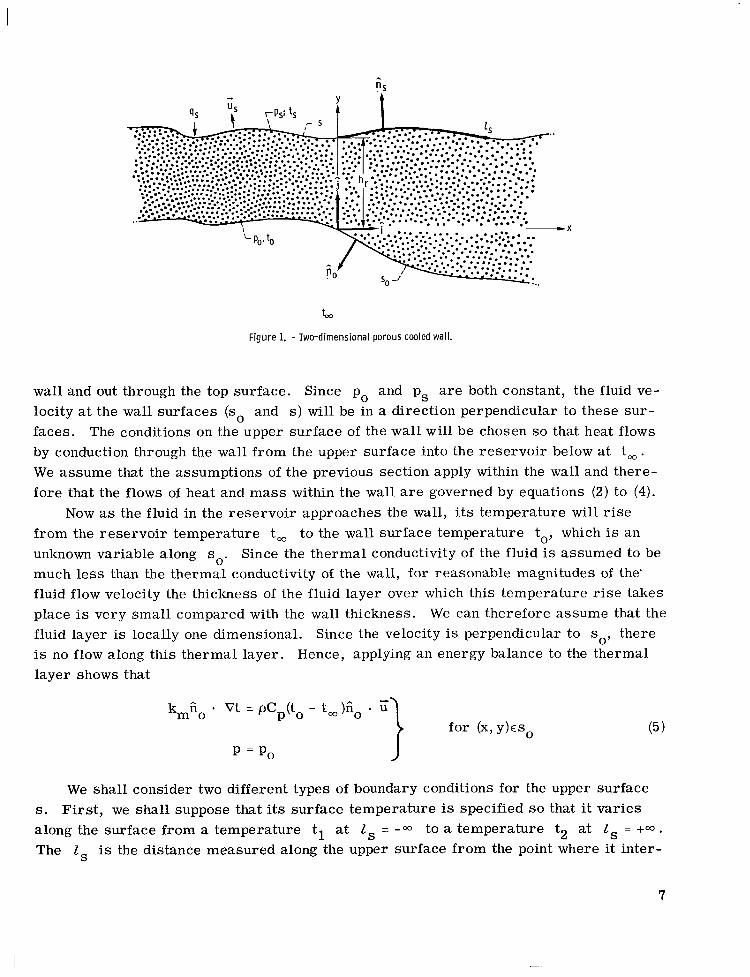
Now consider the two-dimensional porous wall shown in figure 1. The lower surface of the wall whose unit outward-drawn normal is go is denoted by so, and the upper sur - face of the wall whose unit outward-drawn normal is ; is denoted by s. We suppose that no changes occur in the direction perpendicular to the x, y-plane. there is a reservoir which is maintained at constant pressure and temperature po and t, , respectively. The pressure in the fluid above the wall is constant and equal to ps. We suppose that po > p,.

S Below the wall

Then the fluid flows from the reservoir through the porous

6

" S

t,

Figure 1. - Two-dimensional porous cooled wall.

wall and out through the top surface. Since po and ps are both constant, the fluid velocity at the wall surfaces (so and s ) will be in a direction perpendicular to these sur - faces. The conditions on the upper surface of the wall will be chosen so that heat flows by conduction through the wall from the upper surface into the reservoir below at t, . We assume that the assumptions of the previous section apply within the wall and therefore that the flows of heat and mass within the wall are governed by equations (2) to (4).

Now as the fluid in the reservoir approaches the wall, its temperature will rise from the reservoir temperature t, to the wall surface temperature to, which is an unknown variable along so. Since the thermal conductivity of the fluid is assumed to be much less than the thermal conductivity of the wall, for reasonable magnitudes of the' fluid flow velocity the thickness of the fluid layer over which this temperature r i s e takes place is very small compared with the wal l thickness. We can therefore assume that the fluid layer is locally one dimensional. is no flow along this thermal layer. layer shows that

Since the velocity is perpendicular to so, there Hence, applying an energy balance to the thermal

kmiio * V t = pCp(to - t,)no u for (X,Y)ES0 (5 )

P = Po

We shall consider two different types of boundary conditions for the upper surface s. First, we shall suppose that its surface temperature is specified so that it var ies along the surface f rom a temperature tl at 1 , = -00 to a temperature t2 at 1, = +a.

The 1, is the distance measured along the upper surface from the point where it inter-

7

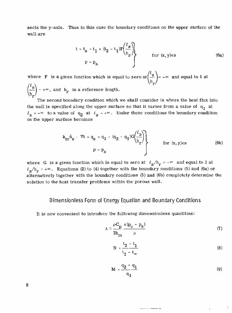
sec ts the y-axis. Thus in this case the boundary conditions on the upper surface of the wall are

P = Ps J where F is a given function which is equal to ze ro at - = - m and equal t o 1 at t)

= +,, and hr is a reference length.

The second boundary condition which we shall consider is where the heat flux into the wall is specified along the upper surface so that it var ies from a value of q1 at I = -, to a value of q2 at I s = +,. Under these conditions the boundary condition on the upper surface becomes

Q S

where G is a given function which is equal to zero a t Zs/hr = -00 and equal to 1 at Zs/hr = +, . Equations (2) t o (4) together with the boundary conditions (5) and (sa) o? alternatively together with the boundary conditions (5) and (6b) completely determine the solution to the heat t ransfer problems within the porous wall.

Dimensionless Form of Energy Equation and Boundary Conditions

It is now convenient to introduce the following dimensionless quantities :

N = t2 - tl t - t, 1

92 - 91

91 M =

8

X = x/hr

y = Y/hr

Po - P

Po - ps c p =

- P hr u = - K (Po - Ps)

t - t, T =-

A

where

7

[ (tl - t, ) i f boundary condition (sa) applies

* i f boundary condition (6b) applies

Upon substituting these definitions into equations (2) to (4) and boundary conditions (5), (sa), and (6b), we obtain

J N - o - u = o

n A - - VT = 2xiiO - ET} 0

for (X,Y)cS0 cp = o

T = 1 + for (X,Y)eS

c p = l

9

I

or

1

for (X,Y)ES

N

?is - VT = 1 +

Cp = 1

where

- V = i - A a +p ax ay

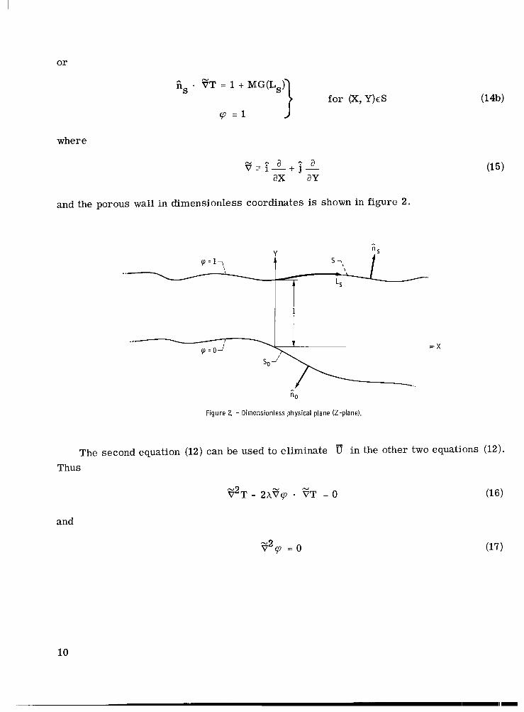
and the porous wall in dimensionless coordinates is shown in figure 2.

The second equation (12) can be used to eliminate v' in the other two equations (12). Thus

and

(17) -2 v q = o

10

Since cp is constant on So and S, it is clear that

N

for (X,Y)cS0

and

N

- vcp for (X,Y)ES ns -- *

I % I Using these resul ts together with the second equation (12) in the boundary conditions (13) and (14b), we obtain

and

q = l J Transformat ion of Boundary Value Problem In to Potential Plane

Since equation (17) shows that q satisfies Laplace's equation, there must exist a harmonic function +b and an analytic function W of the complex variable

such that

W = + b + i q

Physically the change in +b between any two points is proportional to the volume flow of liquid crossing any curve joining those two points. Hence +b must vary between - m

and +a as X varies between -m and +a. Since

9mw = 0 for ZES,

11

and I

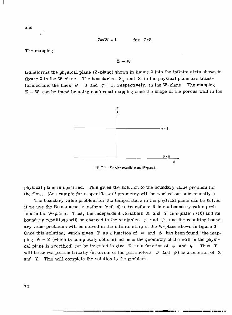
Anw = 1 for ZES

The mapping

z - w

transforms the physical plane (Z-plane) shown in figure 2 into the infinite s t r ip shown in figure 3 in the W-plane. The boundaries So and S in the physical plane are transformed into the lines cp = 0 and cp = 1, respectively, in the W-plane. The mapping Z - W can be found by using conformal mapping once the shape of the porous wall in the

9

Cp'l I

Figure 3. -Complex potential plane (W-plane).

physical plane is specified. the flow.

The boundary value problem for the temperature in the physical plane can be solved i f we use the Boussinesq transform (ref. 4) to transform it into a boundary value problem in the W-plane. Thus, the independent variables X and Y in equation (16) and its boundary conditions will be changed to the variables cp and I), and the resulting bound- a r y value problems will be solved in the infinite s t r ip in the W-plane shown in figure 3 . Once this solution, which gives T as a function of cp and q has been found, the mapping W - Z (which is completely determined once the geometry of the wall in the physical plane is specified) can be inverted to give Z as a function of cp and *. Thus T will be known parametrically (in te rms of the parameters cp and 1c/) as a function of X and Y. This will complete the solution to the problem.

This gives the solution to the boundary value problem for (An example for a specific wall geometry will be worked out subsequently. )

12

---- .. .

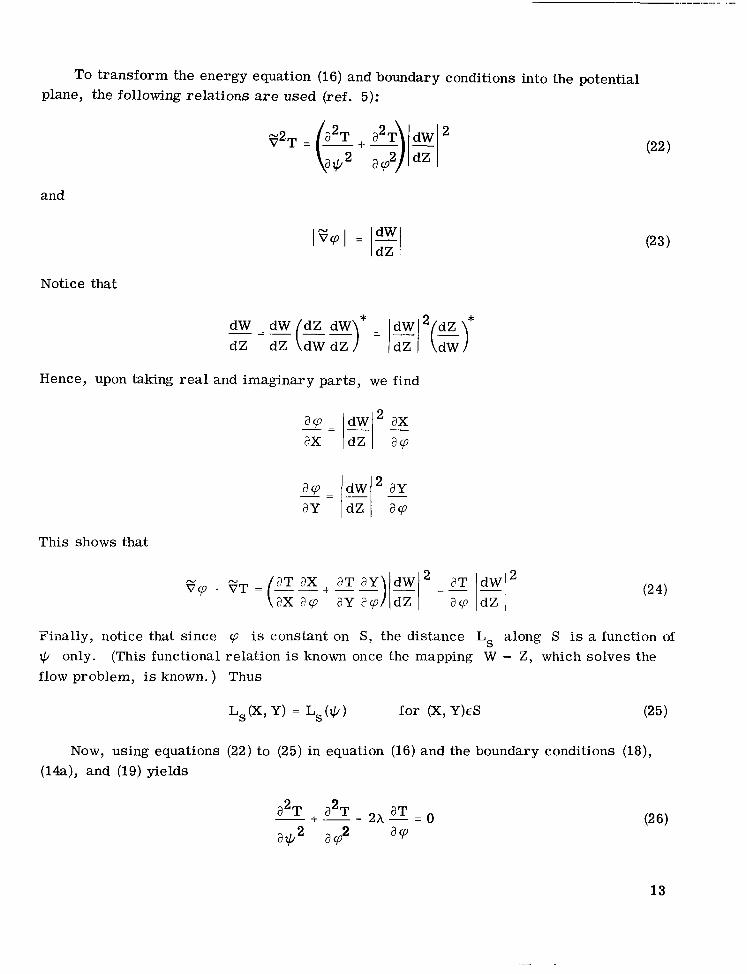
To transform the energy equation (16) and boundary conditions into the potential plane, the following relations are used (ref. 5):

and

2

dZ

Notice that

Hence, upon taking real and imaginary parts, we find

This shows that

Ziiially, notice that since p is constant on S, the distance Ls along S is a function of + only. flow problem, is known. ) Thus

(This functional relation is known once the mapping W - Z, which solves the

Now, using equations (22) to (25) in equation (16) and the boundary conditions (18), (14a), and (19) yields

aT 2 x - = o & + - - a2T

13

or

or

_.- aT 2hT = O for cp = 0 acp

T = 1 -F NF(Ls(q)) for cp = 1

3 = lgl [l + MG(Ls(+))] acp dW

for cp = 1

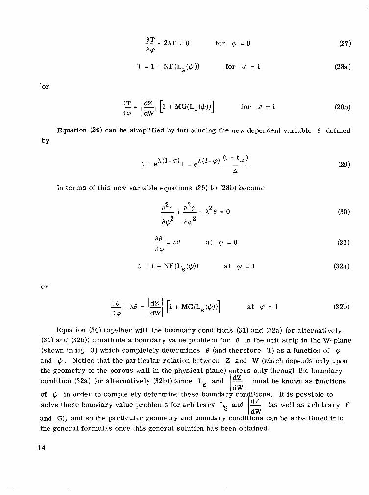
Equation (26) can be simplified by introducing the new dependent variable 0 defined

In te rms of this new variable equations (26) to (28b) become

a2e a2e h2e = - + - -

at c p = O ae acp - = he

6 = 1 + NF(Ls(IC/)) a t cp=1

Equation (30) together with the boundary conditions (31) and (32a) (or alternatively and (32b)) constitute a boundary value problem for 8 in the unit s t r ip in the W-plane

(shown in fig. 3) which completely determines 0 (and therefore T) as a function of ,p and +. Notice that the particular relation between Z and W (which depends only upon the geometry of the porous wall in the physical plane) enters only through the boundary

must be known as functions condition (32a) (or alternatively (32b)) since Ls and

of sl/ in order to completely determine these boundary conditions. It is possible to solve these boundary value problems for arbi t rary Ls and

and G), and so the particular geometry and boundary conditions can be substituted into the general formulas once this general solution has been obtained.

151 (as well as arbi t rary F IgI

14

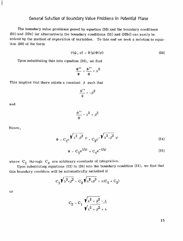
General Solut ion of Boundary Value Problems in Potential Plane

The boundary value problems posed by equation (30) and the boundary conditions (31) and (32a) (or alternatively the boundary conditions (31) and (32b)) can easily be solved by the method of separation of variables. tion (30) of the form

To this end we seek a solution to equa-

Upon substituting this into equation (30), we find

*" a" 2 - + - = A * a

This implies that there exists a constant p such that

and

Hence, I ,-

where C1 through C4 a r e arbi t rary constants of integration.

this boundary condition will be automatically satisfied i f Upon substituting equations (33) to (35) into the boundary condition (31), we find that

c1 d s - c2m = X ( C I + C2)

or

c - c 4 x 2 + p2 - h

2 - l i 2 2 x + p + A

15

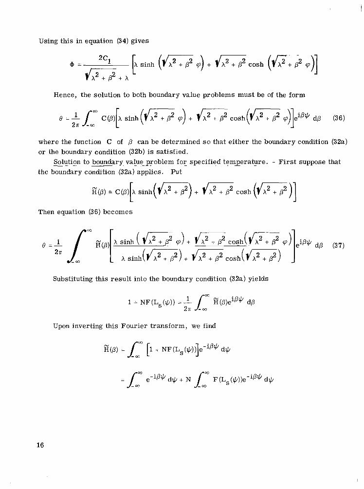
Using this in equation (34) gives

Hence, the solution to both boundary value problems must be of the form

where the function C of p can be determined s o that either the boundary condition (32a) or the boundary condition (32b) is satisfied.

the boundary condition (32a) applies. Solution to boundary value - _ ~ _ problem for - specified . temperature. . _ - - First suppose that

Put

L

Then equation (36) becomes

Substituting this result into the boundary condition (32a) yields

1 + NF(Ls(+)) = - Jl" E(p)eipq dp 271

Upon inverting this Fourier transform, we find

16

The first definite integral is equal to

where 6 is the Dirac delta function. Hence

3 P ) = 2716(P) + N H ( P )

where

(38)

(3 9)

Substituting equation (38) into equation (37) yields

Thus equation (40) with H defined in t e rms of the dimensionless temperature dis-

In this case it is also of interest to have an expression for the conduction heat flux tribution F by equation (39) is the solution to the boundary value problem.

qs crossing into the surface S, that is,

qs = k 6 V t for (X,Y)ES m s

Therefore for (X, Y)ES, by use of equations (24) and (23),

dW dZ

Hence, by use of the transformation (29) and the fact that cp = 1 on the boundary S we find

17

Upon substituting equations (32a) and (40) into this expression, we obtain f

+ELm 27T

h -

h

cosh (m) sinh (m)

+ -

+

sinh (m) - - - ---]dl

cosh( dx2,p2) L

Solution to boundary value problem for specified heat flux. - Now suppose that the boundary condition (32b) applies. Put

+ p2) sinh (m) + 2h cosh (m)] L

Then equation (36) becomes

ipIc/ dp

(43 )

e =- 271

(2h2 + p2) sinh

Substituting this result into the boundary condition (32b) yields

Upon inverting this Fourier transform, we obtain

= l- (44)

Thus equation (43) with E" defined in t e rms of the dimensionless heat flux distribution G and the reciprocal surface velocity by equation (44) is the solution to this

18

boundary value problem. (on S) is given by evaluating equations (29) and (43) at cp = 1 to obtain

In particular the upper surface temperature distribution ts

3

4 5

h sinh()/ha+) + c o s h ( m ) iP+ dp (45)

+ p 2 ) s i n h ( m ) + 2 h m

, r p = 1

2

r p = 0 Q ,' 1-

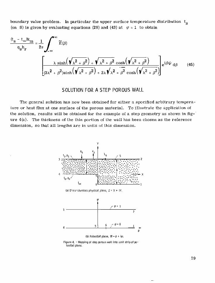
SOLUTION FOR A STEP POROUS WALL

The general solution has now been obtained for either a specified a rb i t ra ry temperature or heat flux at one surface of the porous material. the solution, resul ts will be obtained for the example of a s tep geometry as shown in fig-' u re 4(a). dimension, s o that all lengths are in units of this dimension.

To illustrate the application of

The thickness of the thin portion of the wall has been chosen as the reference

(a) Dimensionless physical plane, Z = X t iY

19

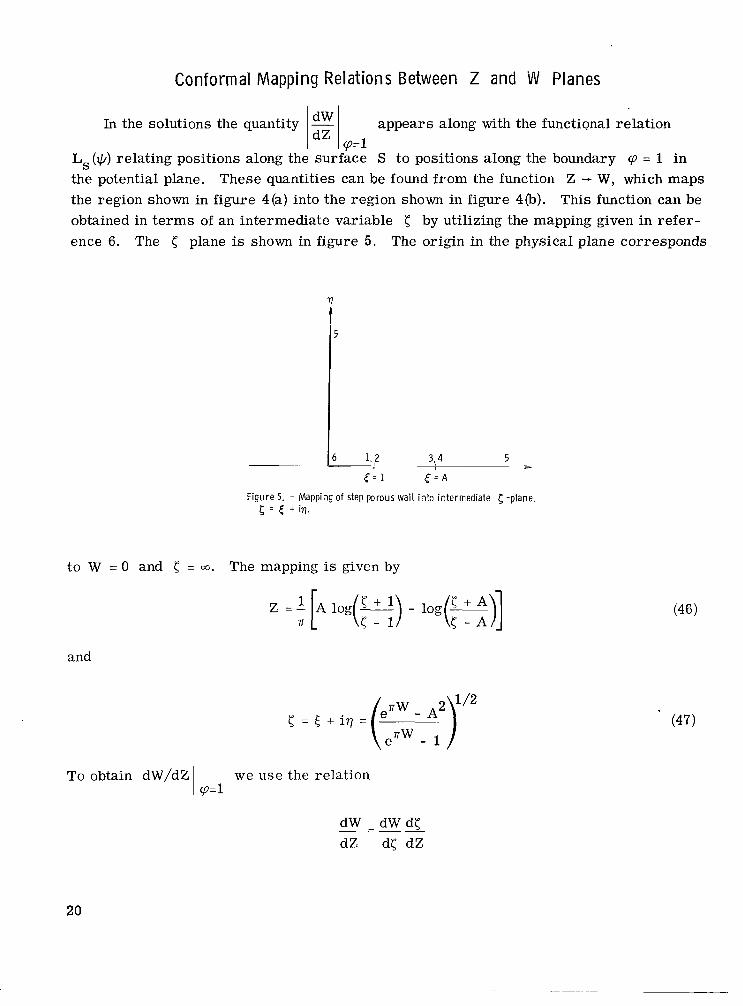
Conformal Mapping Relat ions Between Z and W Planes

appears along with the functional relation Q=1

In the solutions the quantity

Ls(q) relating positions along the surface S to positions along the boundary the potential plane. These quantities can be found from the function Z - W, which maps the region shown in figure 4(a) into the region shown in figure 4(b). This function can be obtained in t e rms of an intermediate variable < by utilizing the mapping given in reference 6. The < plane is shown in figure 5. The origin in the physical plane corresponds

= 1 in

-. 3,,4 5

E = 1 & = A

Figure 5. - Mapping of step porous wall into intermediate -plane, 5 = + ig.

to W = 0 and 5 = co. The mapping is given by

Z = - [ Alog ( c - + 1) - log(r’)] rl 5 - 1 5 - A

and

To obtain dW/dZ we use the relation

dW - dW dc dZ d< dZ

20

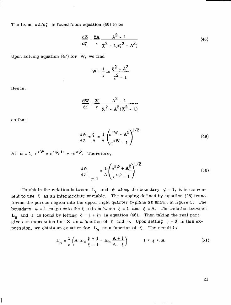
The t e rm dZ/dc is found from equation (46) to be

dZ - 2A

de

A2 - 1 - -- rr (c2 - 1)(c2 - A2)

Upon solving equation (47) for W, we find

1 c 2 - A2 W = - l n

Hence,

A2 - 1 dW - 2c

d5 ' (C2 - A ) (< - 1) 2 2

s o that

At cp = 1, erw = e'*ei' = -e'*. Therefore,

To obtain the relation between Ls and + along the boundary cp = 1, it is convenient to use < as an intermediate variable. The mapping defined by equation (46) transforms the porous region into the upper right quarter <-plane as shown in figure 5 . The boundary cp = 1 maps onto the 5-axis between 5 = 1 and ( = A. The relation between Ls and ( is found by letting 5 = 5 + iq in equation (46). gives an expression for X as a function of ( and q. Upon setting q = 0 in this expression, we obtain an equation for Ls as a function of (.

Then taking the real par t

The result is

I

21

The relation between .$ and I) along Ls is found from equation (47) by letting 71 = 0 and cp = 1 to obtain

vs =

Thus equations (51) and (52) a r e parametric equations that re la te Ls to I,L.

acp ay -

cp=1

Exit Veloci ty From Porous Plate

It follows from equations (12) and (15) that for this example the velocity of the fluid leaving the porous wall is

Since the fact that cp is constant along the upper boundary implies that acp/aX = 0,

It therefore follows from equation (50) that

Solu t ion f o r a Step in Wal l Temperature

(53)

In order to demonstrate how equation (42) can be applied, specific resul ts will now be obtained for the example of a step function wall temperature variation along the boundary S. This solution also yields for zero s tep height the case of uniform wall temperature. In particular, let ts change from tl to t2 at an arbi t rary location Lg so that the boundary condition (14a) becomes

22

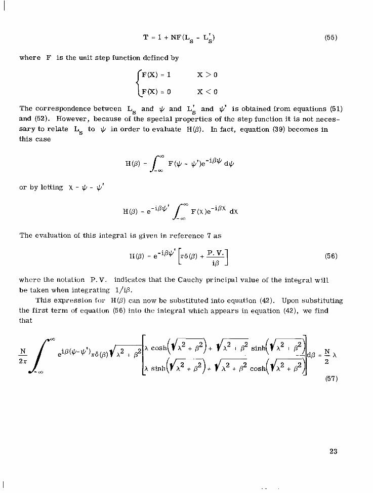
T = 1 + NF(Ls - Lk) (55)

where F is the unit s tep function defined by

F(X) = 1 x > o { F(X) = 0 x < o The correspondence between Ls and +b and LA and +b' is obtained from equations (51) and (52). However, because of the special properties of the s tep function it is not neces- s a r y to relate Ls to +b in order to evaluate I€@). In fact, equation (39) becomes in this case

or by letting X = Q - so'

The evaluation of this integral is given in reference 7 as

where the notation P . V . indicates that the Cauchy principal value of the integral will be taken when integrating l/i/3.

This expression for H(p) can now be substituted into equation (42). the first te rm of equation (56) into the integral which appears in equation (42), we find that

Upon substituting

N 2

cosh()/X2 + p2) + d G sin.( )/A2 + p2) dp = - A

s i n h ( m ) + dX2 + p2 cosh(dX2 + pa) 1 (57)

03

e 277

23

integral yields the expression

-

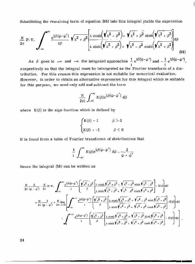
Substituting the remaining te rm of equation (56) into this

(58)

N 28

'p(+-$') and - - 1 eiP(Ic;-Ic;') A s p goes to 100 and -00 the integrand approaches - e 7

i i respectively so that the integral must be interpreted as the Fourier transform of a distribution. For this reason this expression is not suitable for numerical evaluation. However, in order to obtain an alternative expression for this integral which is suitable for this purpose, we need only add and subtract the t e rm

where E(p) is the sign function which is defined by

It is found from a table of Fourier transforms of distributions that

Hence the integral (58) can be written as

--+-P.V. N 2 N f m e { fl [ X c o s h m . m s i n h ) l h 2 + P 2 1- E @ b

A sinh- + cosh- 27r (9- *') 28

-03

24

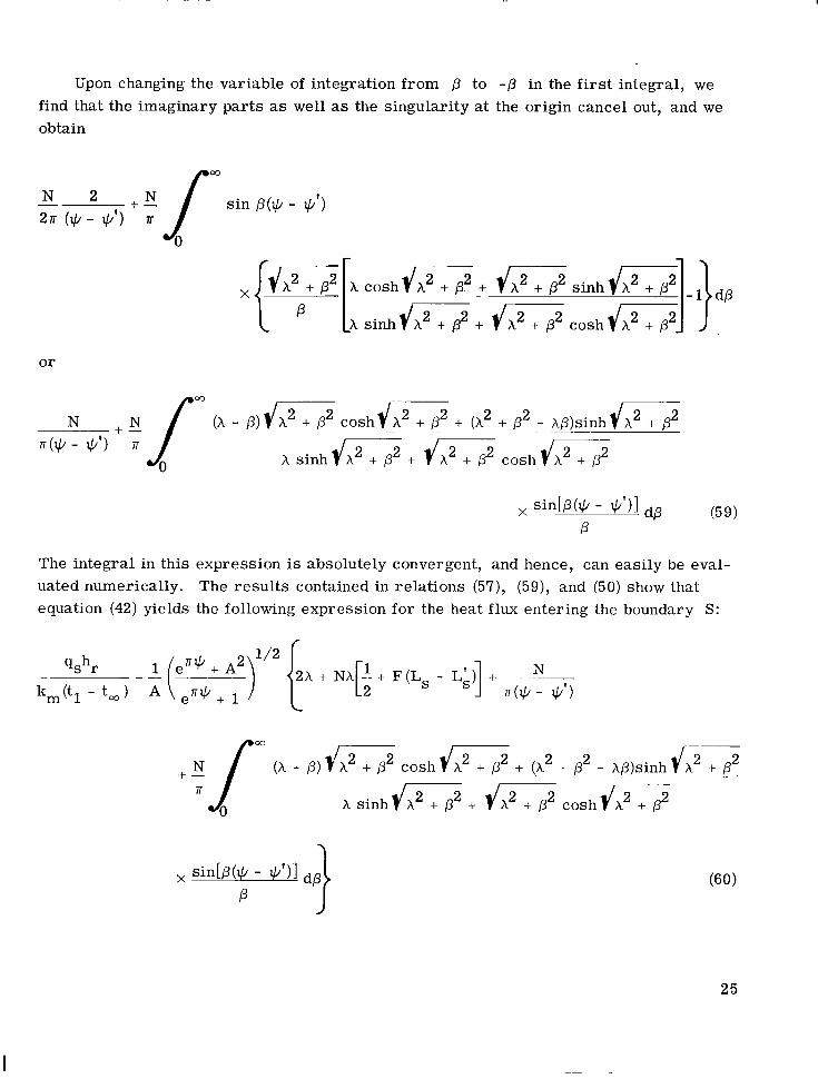
Upon changing the variable of integration from P to -/3 in the first integral, we find that the imaginary par ts as well as the singularity at the origin cancel out, and we obtain

or

m

(A - P)) /h2 + P2 cosh)/J2 + P 2 2 2 + (h + P - hP)sinh

h sinh)/h2 + P2 + c o s h d m

N

The integral in this expression is absolutely convergent, and hence, can easily be evaluated numerically. equation (42) yields the following expression for the heat flux entering the boundary S:

The resul ts contained in relations (57), (59), and (50) show that

00

+ (A2 + P2 - XP)sinh

h s i n h d G + d G cosh d h 2 + p2 A

2 5

Solution for Uniform Heat Flux

In order to illustrate how equation (45) is applied, consider the case where a uniform heat flux is imposed along the surface S. The function G in equation (6b) is zero in this instance, and equation (50) gives an expression for dW/dZ . Hence in this case the I @=I

- I - function E" in equation (44) is given by

As * - m the integrand goes to e -ip* and as + - -00 the integrand goes to e-iB*/A, so that this integral exists only as the Fourier transform of a distribution and not as an ordinary integral. In order to separate out the singular parts of this integral, notice that equation (61) can be written as

where the first two integrals a r e absolutely convergent and the last two integrals can be evaluated from a table of Fourier transforms to give

-1 - 1 27r6(P) + (1 - L)[n6(8) +

A A i P

Thus the following expression for is obtained

26

This is now inserted into equation (45). We shall consider the integrals resulting from the various te rms of equation (62) individually. t e rm of equation (62) is

The integral resulting from the first

I- -

= ($ + +) X sinh X + X cosh X - -- A + l 2 2 4X 2 X sinh X + 2 X cosh X

The integral resulting from the second te rm of equation (62) is

This latter integral is absolutely convergent. Now consider the integrals resulting from inserting the last two t e rms of equation (62) into equation (45). These integrals a r e also found to be absolutely convergent. The exponential t e rms in the integrals can therefore be expressed in trigonometric form. After collecting rea l and imaginary parts, it is found that the imaginary part of the integrand is an odd function of p so that its integral from /3 = --oo to -oo is zero. The integral of the remaining rea l part can be expressed as an integral from p = 0 to -oo and is then combined with equations (63) and (64) to yield the following expression for the surface temperature :

+ E(p, +) [ cosh- + X sinh X + @ ]dp (65a) n

27

where

DISCUSSION

A general analytical method has been presented for determining the heat t ransfer characterist ics of two-dimensional porous cooled media. This method is based on transforming the energy equation so that its independent variables a r e the coordinates in the potential plane for the fluid flow. The energy equation is separable in these coordinates, and hence a general solution can be obtained. A feature that aids in the solution is that the boundaries of the porous material are at constant pressure and as a consequence they map into parallel constant velocity potential lines in the complex potential plane. provides a convenient region in which to solve the energy equation. potential plane is then related to the physical plane by conformal mapping between the two regions.

The following discussion concerns the application of the solution to the example of a porous wall with a s tep change in cross section. No attempt is made to conduct a parametric study to demonstrate the effect of the governing dimensionless parameters since this would only be of practical value if a particular engineering application were in mind.

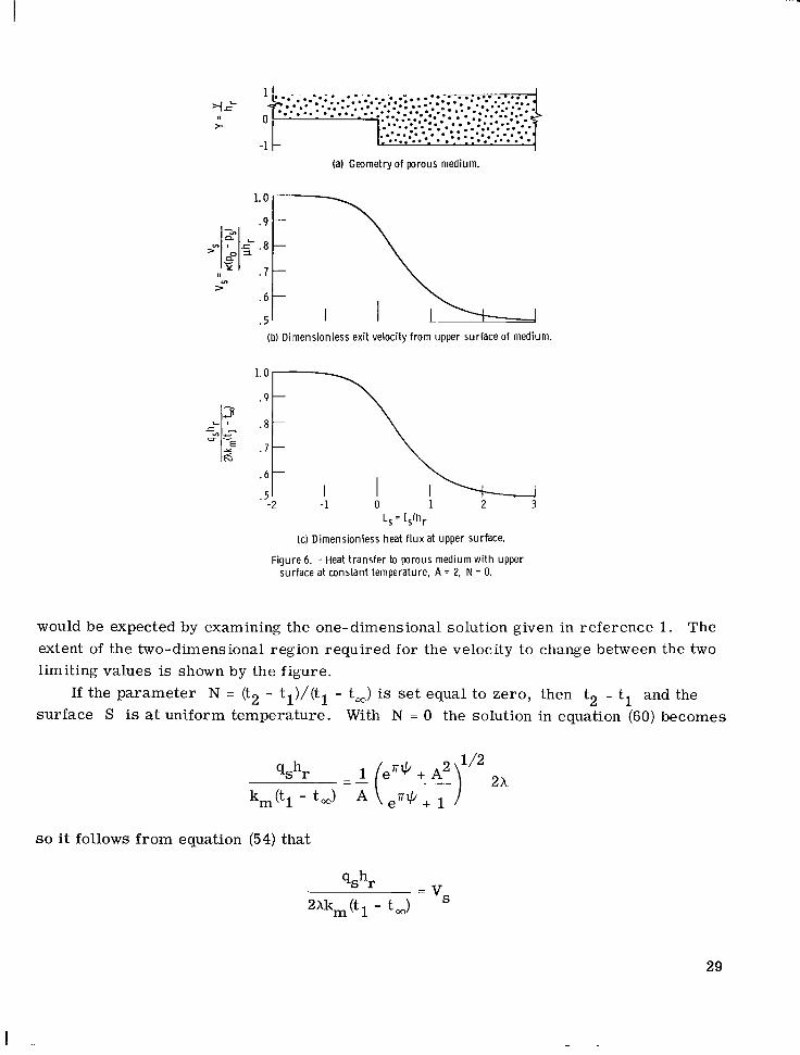
dimensionless heat flux into the boundary S of the porous material parametrically as a function of position when the temperature distribution is a step function along that sur - face. The result contains the parameters X, N, +', and A. The parameter A is the ratio of the thicknesses of the two regions of the porous wall as shown in figure 4(a). only resul ts which will be presented a r e for a value of A equal to 2. Hence, the geom- e t ry will always be as shown in figure 6(a). The heat flux is first computed as a function of I) from equation (60). It is then expressed as a function of the coordinate Ls along the surface by use of the correspondence between Ls and I) given by equations (51) and (52).

The dimensionless velocity leaving the upper surface is given by equation (54) and is shown in figure 6(b) for the porous plate with a s tep ratio A of 2. At the l imits of large negative Ls and large positive Ls the velocity V, goes, respectively, to 1 and 1/2, as

This The solution in the

Consider now the solution given by equations (51), (52), and (60). They give the

The

(a) Geometry of porous medium.

(b) Dimensionless exit velocity from upper surface of medium.

Ls = Zs/hr

(c ) Dimensionless heat f lux at upper surface.

Figure 6. -Heat t ransfer to porous medium with upper surface at constant temperature, A = 2, N = 0.

would be expected by examining the one-dimensional solution given in reference 1. The extent of the two-dimensional region required for the velocity to change between the two limiting values is shown by the figure.

If the parameter N = (t2 - tl)/(tl - t,) is set equal to zero, then t2 = tl and the surface S is at uniform temperature. With N = 0 the solution in equation (60) becomes

2x qshr - _ - 1 (e"+ + A

s o it follows from equation (54) that

29

I

Thus for a given porous matrix when the surface temperature is uniform, the dimensionless heat flux into the boundary is directly proportional to the fluid exit velocity. The dimensionless heat flux is shown in figure 6(c). This curve is the same as the curve in figure 6(b).

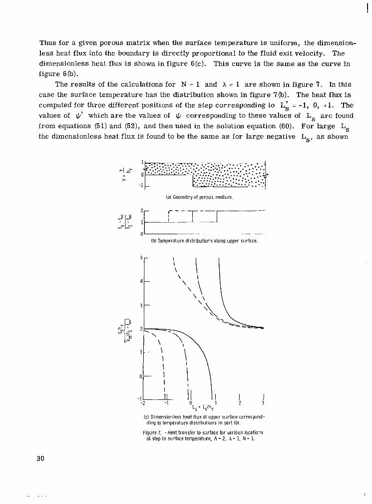
The resul ts of the calculations for N = 1 and h = 1 a r e shown in figure 7. In this case the surface temperature has the distribution shown in figure 7(b). The heat flux is computed for three different positions of the step corresponding to LA = -1, 0, +l. The values of Q' which a r e the values of Q corresponding to these values of Ls a r e found from equations (51) and (52), and then used in the solution equation (60). For large Ls the dimensionless heat flux is found to be the same as for large negative Ls, as shown

(a) Geometryof porous medium.

_ _ __ ~~ ... . 0 ' (b) Temperature distributions along upper surface.

(c) Dimensionless heat f lux at upper surface cor respnd-

Figure 7. - Heat transfer to surface for various locations

ding to temperature distributions i n part (b).

of step i n surface temperature, A = 2, A = 1, N = 1.

30

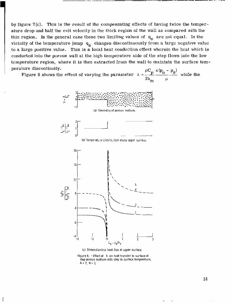
by figure 7(c). a ture drop and half the exit velocity in the thick region of the wall as compared with the thin region. In the general case these two limiting values of qs a r e not equal. vicinity of the temperature jump qs changes discontinuously from a large negative value to a large positive value. This is a local heat conduction effect wherein the heat which is conducted into the porous wall at the high temperature side of the s tep flows into the low temperature region, where it is then extracted from the wall to maintain the surface temperature discontinuity .

This is the result of the compensating effects of having twice the temper-

In the

PCP K(Po - Ps>

2km P Figure 8 shows the effect of varying the parameter h =- while the

(a) Geometryof porous medium.

q - 8 -* --

0 (b) Temperature distribution along upper surface,

(c) Dimensionless heat f lux at upper surface,

Figure 8. - Effect of A on heat transfer to surface of step porous medium with step in surface temperature, A - 2, N = 1.

31

temperature distribution on the wall surface remains fixed as given in figure 8(b). The larger values of h a r e associated for example with larger pressure differences po - ps and hence with larger flows. Thus to maintain a fixed surface temperature, the heat flux into the plate can be increased when the flow is increased to correspond to a larger value of A.

Now consider the solution given by equations (51), (52), and (65) for the case of uniform heat input at the surface S. There a r e only two parameters involved, A and A. Numerical results have been obtained for A = 2, and they are shown in figure 9. The exit velocity Vs is the same as in figure 6 and is repeated here for convenience in in-

(a) Geometry of porous medium.

(b) Dimensionless exit velocity from upper surface of medium.

0 I 1 I -2 -1 0 1 2 3

L,= Zs/hr

(cJ Temperature of upper surface.

Figure 9. - Effect of h on surface temperature for im-

.lL I

posed uni form heat flux, A = 2.

32

... - ................. I , . . , , I,,,,,, I I I I 11111 I I I

terpreting the results. Since X increases when the flow through the wall increases, the temperature difference ts - t, between the surface and the reservoir decreases as X

is increased for a fixed qs. Note that qs has been combined into the dimensionless ordinate of figure 9(c) s o that each curve can be used for any value of qs. As would be expected, the regions of high surface temperature are associated with the regions of low exit velocity.

The preceding resul ts serve to illustrate the type of heat transfer behavior to be expected in a two-dimensional porous configuration.

CONCLUSIONS

An analytical approach has been developed for obtaining the heat transfer behavior in a two-dimensional porous material . The method depends on the fact that the surfaces of the porous material at the inlet and outlet of the coolant are each at constant pressure. For the type of flow involved, the dimensionless pressure can be regarded as a velocity potential, and as a consequence the porous region maps into a simple s t r ip in the complex potential plane. The energy equation was transformed into the potential plane, and a general solution was obtained. This solution can be applied to any wall geometry by finding the appropriate conformal map of the s t r ip in the potential plane into the physical plane.

specific case of a step porous wall which is made up of two regions, each having a different uniform thickness.

The analytical technique was applied for various imposed thermal conditions in the

Lewis Research Center, National Aeronautics and Space Administration,

Cleveland, Ohio, April 9, 1970, 129-01.

REFERENCES

1. Schneider, Paul J. : Conduction Heat Transfer. Addison-Wesley Publ. Co. , Inc., 1955.

2. Grootenhuis, P. : The Mechanism and Application of Effusion Cooling. J. Roy. Aeron. SOC., vol. 63, no. 578, Feb. 1959, pp. 73-89.

33

I l1ll11l1111

3. Koh, J. C. Y. ; and del Casal, E. : Heat and Mass Flow Through Porous Matrices for Transpiration Cooling. Proceedings of the 196 5 Heat Transfer and Fluid Mechanics Institute. Andrew F. Charwat, ed. , Stanford Univ. Press, 1965, pp. 263-281.

4. Boussinesq, J. : Calcul du Pouvoir Refroidissant des Courants Fluides. J. Math. &res et Appl., vol. 1, 1905, pp. 285-332.

5. Churchill, Rue1 V. : Complex Variables and Applications. Second ed., McGraw-Hill Book Co., Inc. , 1960.

6. Milne-Thomson, Louis M. : Theoretical Hydrodynamics. Second ed., Macmillan Co., 1950.

7. Papoulis, Athanasios: The Fourier Integral and Its Applications. McGraw-Hill Book Co., Inc., 1962.

34 NASA-Langley, 1970 - 33 E-5526

~ - ~~ ~~ I

NATIONAL AERONAUTICS AND SPACE ADMINISTRATION WASHINGTON, D. C. 20546

OFFICIAL BUSINESS FIRST CLASS MAIL

POSTAGE A N D FEE NATIONAL AERONAU

SPACE ADMINISTR.

09U 001 5 8 51 30s 70185 00903

A I R FORCE WEAPONS L A B O R A T O R Y /WLOL/ K I R T L A N D AFB, NEW M E X I C O 87117

"The aeronairiical and space nctivities of the Uizited States shall be condifcted so as io contribuie . . . i o the expansioiz of hziiiiaiz k n o d edge of phenonieiza in the ntiiiosphere and space. T h e Adniinistrntion shall provide for the widest prncticable nnd appropriate dissemination of inforiiiniion concerning i ts nciiirities and ihe ~ e s ~ l i s ihereof."

-NATIONAL AERONAUTICS AND SPACE ACT OF 1958

NASA SCIENTIFIC AND TECHNICAL PUBLICATIONS

TECHNICAL REPORTS: Scientific and technical information considered important, complete, and a lasting contribution to existing knowledge.

TECHNICAL NOTES: Information less broad in scope but nevertheless of importance as a contribution to existing knowledge.

TECHNICAL MEMORANDUMS: Information receiving limited distribution because of preliminary data, security classifica- tion, or other reasons.

CONTRACTOR REPORTS: Scientific and technical information generated under a NASA contract or grant and considered an important contribution to existing knowledgc.

* .

TECHNICAL TRANSLATIONS: Information published in a foreign language considered to merit NASA distribution in English.

SPECIAL PUBLICATIONS: Information derived from or of value to NASA activities. Publications include conference proceedings, monographs, data compilations, handbooks, sourcebooks, and special bibliographies.

TECHNOLOGY UTILIZATION PUBLICATIONS: Infofmation on technology used by NASA that may be of particular interest in commercial and other non-aerospace application$. Publications include Tech Briefs, Technology Utilization Reports and Notes, and Technology Surveys.

Details on the availability of ihese publications may be obtained from:

SCIENTIFIC AND TECHNICAL INFORMATION DIVISION

NATIONAL AERONAUTICS AND SPACE ADMINISTRATION Washington, D.C. 20546

I .. . . . - 1 1 1 1 1 1 1 II I I I I ~ ~ .---- - . .. II . . ~ . - - . -- .... ... ...-- .,11. .111 I I 11.1

analytical method for steady state heat transfer in two

Documents