Analytical Model for High Level Power Modelingof Combinational and Sequential Circuits†

Subodh Gupta and Farid N. Najm

ECE Dept. and Coordinated Science Lab.University of Illinois at Urbana-Champaign

Urbana, Illinois 61801

Abstract

In this paper, we propose a modeling approach that captures the dependence of the power dissipa-tion of a (combinational or sequential) logic circuit on its input/output signal switching statistics.The resulting power macromodel, consists of a quadratic or cubic equation in four variables, thatcan be used to estimate the power consumed in the circuit for any given input/output signal statis-tics. Given a low-level (typically gate-level) description of the circuit, we describe a characteriza-tion process that uses a recursive least squares (RLS) algorithm by which such a equation-basedmodel can be automatically built. The four variables of our model are the average input signalprobability, average input switching activity, average input spatial correlation coefficient and av-erage output zero-delay switching activity. This approach has been implemented and models havebeen built and tested for many combinational and sequential benchmark circuits.

1. IntroductionWith the advent of portable and high-density micro-electronic devices, the power dissipation of

very large scale integrated (VLSI) circuits has become a critical concern. Modern microprocessorsare hot, and their power consumption can exceed 30 or 50 Watts. Due to limited battery life,reliability issues, and packaging/cooling costs, power consumption has become a more criticaldesign concern than speed and area in some applications. Hence to avoid problems associatedwith excessive power consumption, there is a need for CAD tools to help in estimating the powerconsumption of VLSI designs.

A number of CAD techniques have been proposed for gate-level power estimation (see [1] fora survey). However, by the time the design has been specified down to the gate level, it may betoo late or too expensive to go back and fix high power problems. Hence in order to avoid costlyredesign steps, power estimation tools are required that can estimate the power consumption ata high level of abstraction, such as when the circuit is represented only by the Boolean equations.This will provide the designer with more flexibility to explore design trade-offs early in the designprocess, reducing the design cost and time.

In response to this need, a number of high-level power estimation techniques have beenrecently proposed (see [2] for a survey). Two styles of techniques have been proposed, which werefer to as top-down and bottom-up. In the top-down techniques [3, 4], a combinational circuitis specified only as a Boolean function, with no information on the circuit structure, number ofgates/nodes, etc. Top-down methods are useful when one is designing a logic block that was notpreviously designed, so that its internal details are unknown.

In contrast, bottom-up methods [5–11] are useful when one is reusing a previously-designedlogic block, so that all the internal structural details of the circuit are known. In this case, onedevelops a power macromodel for this block which can be used during high-level power estimation(of the overall system in which this block is used), in order to estimate the power dissipation ofthis block without performing a more expensive gate-level power estimation on it.

The method in [5] uses the power factor approximation technique, which treats all the circuitinput bits as digital “white noise” and due to this assumption can give errors of up to 80% incomparison to gate-level tools. Although [6] gives more accurate result, its main disadvantageis that it treats different modules differently, requiring specialized analytical expressions for thepower to be provided by the user. Thus, depending upon the functionality of the module, adifferent type of macromodel (analytical equation) may have to be used.

The method in [7] characterizes the power dissipation of circuits based on input transitionsrather than input statistics. Since the number of possible input transitions for an n-input com-binational circuit is 22n, they present a clustering algorithm to compress the input transitionsinto clusters of input transitions that have the same power values (approximately). They use

†This research was supported in part by the National Science Foundation (NSF MIP 97-10235) andby the Semiconductor Research Corporation (SRC 97-DJ-484), with technical mentorship from TexasInstruments Inc.

heuristics to implement the clustering algorithm, but it is not clear how efficient the methodwould be on large circuits.

In [8], the authors present a technique to estimate switching activity and power consumptionat the RTL for data path and control circuits, in the presence of glitching activity. To construct apower macromodel, they use both analytical equations and look-up tables. The method is quitegood and uses 9 or more variables in the power macromodel. Our independent work has shownthat it is possible to construct a look-up table power macromodel with much fewer variables (4can be enough).

In [9], the authors presented a macromodel for estimating the cycle-by-cycle power at theRTL. The proposed methodology consists of three steps: module equation form generation andvariable selection, variable reduction, and population stratifications. The generated macromodelhas 15 variables. They show good accuracy in estimating average and cycle-by-cycle power. Themacromodels are dependent on a training vector set, so that the accuracy is compromised if thetraining set is not similar to the vector set to be applied.

All the approaches discussed above are limited to only combinational circuits. In this paper,we propose a power macromodeling approach for both combinational and sequential circuits that(1) takes into account the effect of the circuit input switching activity and does not treat thecircuit inputs as white noise, (2) takes into account input correlation, both spatial and temporaland (3) is based on a single fixed macromodel template which does not depend on the typeof circuit being analyzed. Our model is equation-based. Specifically, we construct a quadraticor cubic equation in the following four variables: average input signal probability (Pin), averageinput switching activity (Din), average input spatial correlation coefficient (SCin), and averageoutput zero delay switching activity (Dout). For a logic node, the switching activity, also calledthe transition density [12], is defined as the average number of logic transitions per unit time.The zero delay switching activity refers to the case when the circuit gates are considered to havezero delay, so that only truly required logic transitions (and no hazards or glitches) are observed.From a high-level view, it is reasonable to assume that fast functional simulation will be appliedto measure signal switching statistics, so that only the zero delay output activity (and not thereal delay output activity) will be computed. The main advantage of our approach is that alltypes of circuits are treated in the same way, i.e., we do not use different model equation types fordifferent modules. As a result, the method is very easy to use, and requires no user intervention.Indeed, we will present an automatic characterization procedure by which the macromodel canbe built for a given circuit.

This paper is organized as follows. In section 2, we will give some background regarding ouroriginal 4-dimensional (4D) table-based macromodel. In section 3, we will explain why the modelholds just as well for sequential circuits. In section 4, we discuss the new analytical-equation-based formulation of the 4D model and describe the characterization procedure. In section 5, wegive empirical results that show the effectiveness of this model, and we summarize and concludein section 6.

2. The 4D tabular macromodelWe have previously presented a 4-dimensional (4D) table-based macromodel in [10, 11, 13] for

combinational circuits. In this paper, we will show that the method extends to sequential circuits;we will also show that the table can be accurately represented by a simple analytical equation,and we will describe the required automatic characterization flow. The 4D macromodel considersthe average power of a circuit to be a function of four variables:

Pavg = f(Pin, Din, SCin, Dout) (1)

These four variables were defined above, but SCin deserves a few more words. SCin is equal tothe average of all the pair-wise spatial correlations SCij between signals xi and xj, where:

SCij = P {xi ∧ xj = 1} (2)

i.e., it is the probability of both inputs being high simultaneously. Even though the joint probabil-ity is not what is usually referred to as “correlation coefficient” between two random variables, inthis case of Boolean variables the joint probability of two bits is enough to capture their completejoint distribution and, therefore, suffices as a measure of their correlation. These four variablesare not independent. Indeed, it was observed in [11, 13] that Pin, Din and SCin should satisfythe following constraints:

Din

2≤ Pin ≤ 1 − Din

2(3)

nP 2in − Pin

(n − 1)≤ SCin ≤ Pin (4)

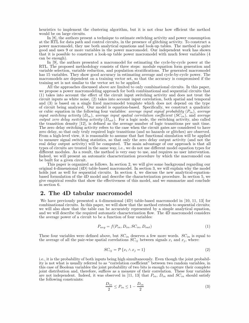
where n is the number of primary inputs.The combined scatter plot of all ISCAS-85 circuits [14] showing the accuracy of the 4D tabular

approach while estimating the total power in presence of correlated input vectors is shown in Fig. 1.The plot reports normalized power values, so that the results for all the circuits can be examinedon the same plot. The results are summarized in Table 1. The average error in all cases is lessthan 10%, which shows the accuracy of this 4D tabular approach.

0.0 0.5 1.0 1.5 2.0Power, from macromodel(uW/MHz/gate)

0.0

0.5

1.0

1.5

2.0

Pow

er, f

rom

sim

ulat

ion(

uW/M

Hz/

gate

)

Figure 1. Power comparison between correlated input vectorstream and 4D macromodel, when total power is estimated.

3. Extension to sequential circuitsAll previous work in this area was restricted to combinational circuits. In this section we will

show that our macromodel extends with ease to sequential circuits. Upon first consideration, itwould seem that primary inputs information is not sufficient to model the power of sequentialcircuits, and that some information on the state bits would have to be required. However, whenthe objective is to estimate the average power, the fact that the state over a long time periodbecomes independent of the initial state leads to significant simplification of the problem. Indeed,it was shown in [15], that if the sequence of inputs to a sequential machine is of order k, then a lag-k Markov chain correctly models the input sequence as well as the k-step conditional probabilitiesof the primary primary inputs and internal states.

As a result, if the input signal temporal correlations die down with time, which is a rea-sonable assumption in practice, then under steady state the state bits distribution is completelydetermined by the primary inputs distribution, and the statistics of the primary inputs shouldbe sufficient to model the power of a sequential circuits. Indeed, we have experimentally foundout that the same 4D macromodel also works for sequential circuits, as will be shown in theexperimental results section below.

4. Equation-based macromodelThe table-based macromodel requires a lot of memory for storing the table and also requires a lotof time to build the whole table. We have developed an alternate approach by which we can fit ageneral non-linear equation to the function f(·) in (1) without user intervention and with muchless time than it takes to fill the table. This general equation is fixed and is used as the startingpoint for all circuits - no user intervention is required in the choice of equation. We will refer tothis equation as the template. This works because, even though the function f(·) is non-linear,it turns out that in practice it is “not too non-linear” to defy fitting, and a general polynomialtemplate turns out to be sufficient.

For efficiency reasons, one would like to use the lowest order polynomial template that works.One option is the linear function:

Pavg = c0 + c1Pin + c2Din + c3SCin + c4Dout (5)

where the coefficients ci are unknown and are to be determined during the characterization usingregression analysis. To estimate the regression variables ci, we generated 1000 blocks of correlatedvector streams for different values of Pin, Din, and SCin, covering a wide range of input statistics.For each block of vectors, Monte Carlo simulation [16] was used to estimate the average powerand to compute the value of Dout. Using this set of data and the standard linear least squaresmethod [17], the regression variables ci were estimated.

To test the accuracy of the fit, we again generated 1000 blocks of correlated input vectorsfor different values of Pin, Din, and SCin. Using Monte Carlo simulation [16], the average power(Pavg) and Dout were estimated. For the given Pin, Din, SCin, and Dout values, the averagepower Pavg was then found using (5) and the relative error between Pavg and Pavg was computedand is shown in Table 2. It is evident from the table that a linear function is not good enoughfor estimating the average power for most of the circuits.

Table 1. Error in the 4D approach,while estimating total power

Circuit Average Error Max.Errorc432 5.56% -27.8%c880 6.7% 50.61%c1908 3.85% 31.17%c2670 7.8% 37.53%c3540 7.5% 44.19%c5315 3.48% 29.03%c6288 9.6% 43.15%c7552 8.95% -45.79%c499 5.96% 46.3%c1355 6.19% 33.56%

Table 2. Average and maximum error when totalpower was estimated using linear function

Circuit Avg. Error Max.Errorc499 36.6% 1407.2%c880 19.7% 257.16%c1355 34.7% 993.9%c1908 11.6% 68.18%c432 11.01% 30.45%c5315 11.4% 89.84%c2670 20.36% 304.6%c3540 13.07% 258.6%c7552 15.5% 85.8%c6288 31.9% 257.16%

To improve the accuracy, another option is the quadratic function:

Pavg = c0 + c1Pin + c2Din + c3SCin + c4Dout

+ c5PinDin + c6PinSCin + c7PinDout + c8DinSCin + c9DinDout + c10SCinDout

+ c11P2in + c12D

2in + c13SC2

in + c14D2out

(6)

Using the same approach as above, the regression variables were estimated and the accuracyof the results was tested and is shown in Table 3. It is evident from the table that the quadraticfunction is better for estimating the average power for most of the circuits except c499 and c1355for which the average error was very high, above 15%.

We also investigated the general cubic form. Due to space limitations, we are not showing thecubic equation here as it consists of 35 coefficients. Table 4 shows the average error and maximumerror for the case of a cubic. It is clear that the improvement in the error is not much for mostof the circuits, except for c499 and c1355 for which the quadratic function did not do well. Thisobservation was found to hold in general, that for many circuits the quadratic model is enough,but the cubic model can still be superior in some cases. As a result, we use a hybrid approachby which we start with the quadratic model by default and increase the order of the model to acubic only if the measured error during characterization is too big. It was observed that the cubicfunction was the highest order function required by all the ISCAS-85 circuits. Similar experimentswere performed on sequential circuits, except that the power was estimated using [18]. It wasobserved that the quadratic function is sufficient for all the sequential circuits that we tested.

Table 3. Average and maximum errorwhen total power was estimated usingthe quadratic model

Circuit Avg. Error Max.Errorc499 25.64% 1319.5%c880 5.9% 48.74%c1355 18.08% 107.9%c1908 4.9% 57.74%c432 4.19% 36.8%c5315 3.6% 32.56%c2670 10.25% 42.25%c3540 5.86% 50.49%c7552 8.8% 50.48%c6288 9.6% 55.74%

Table 4. Average and maximum error whentotal power was estimated using the cubic model

Circuit Avg. Error Max.Errorc499 8.3% 56.06%c880 5.2%% 45.41%c1355 12.07% 50.78%c1908 4.12% 34.31%c432 3.13% 24.16%c5315 3.8% 40.42%c2670 6.25% 39.45%c3540 3.7% 46.38%c7552 5.6% 47.96%c6288 8.3% 54.6%

5. CharacterizationTo derive the analytical expressions discussed above, we have developed an automatic character-ization process using the recursive least squares (RLS) [19] algorithm. RLS is used in adaptive

filtering for on-line estimation of filter parameters. The following summary of the general RLSalgorithm is given for convenience.

5.1. RLS algorithmLet y = f(x1, x2, . . . , xp) be a real valued function of real variables. We will use bold font to

denote vector or matrix quantities. Let the (column) vector x be the vector of the p variables,so that the transpose of x is the (row) vector xT = [x1 x2 · · · xp] and we write y = f(x). Weare interested in approximating f(·) with a closed form analytical expression y = cTu, wherecT = [c0 c1 · · · cm−1] is a vector of constant coefficients whose values are to be determined anduT = [u0 u1 · · · um−1], where each ui is some function of the variables x1, x2, . . . , xp. We wouldlike to find a vector c so that y is a good approximation to y.

To this end, suppose we generate n randomly chosen samples x(1), x(2), . . . ,x(n), from whichwe also compute the corresponding y(i), for i = 1, 2, . . . , n. Consider the error e(i) = y(i) − y(i)and the cumulative error ζ(n) =

∑ni=1 |e(i)|2. One way of finding an appropriate c is to find

one that minimizes the error ζ(n). Typically, the solution will depend on n, and we denote it byc(n). Finding such a c(n) is the traditional problem of least-squares fitting which is solved usingstandard linear regression techniques [17]. The result is that c(n) can be obtained as the solutionto the following system of linear equations:

Φ(n)c(n) = z(n) (7)

where Φ(n) is a m × m matrix, and z(n) is a m× 1 vector, given by:

Φ(n) =n∑

i=1

u(i)uT (i) and z(n) =n∑

i=1

u(i)y(i) (8)

The solution c(n) = Φ−1(n)z(n) is the coefficient vector that minimizes the error ζ(n) overthe observed n samples. In order for y to be a good approximation for y over the whole domainof f(·), we need to use a large number n of samples. It would be desirable to iteratively addmore samples while monitoring the error, but this requires inverting Φ(n) every time. In theRLS algorithm, this problem is overcome by using the matrix inversion lemma which leads toan iterative update mechanism for Φ−1(n) that does not require any matrix inversions [19], asfollows:

1. Initialize Φ−1(0) and c(0)2. For n = 1, 2, . . ., until converged, do:

a. Compute the m × 1 gain vector k(n) as follows:

k(n) =Φ−1(n − 1)u(n)

1 + uT (n)Φ−1(n − 1)u(n)(9)

b. Update the coefficient vector c(n) = c(n − 1) + k(n)[y(n) − cT (n − 1)u(n)

]c. Update the correlation matrix Φ−1(n) =

[I − k(n)uT (n)

]Φ−1(n − 1)

3. End.To use the above algorithm, the initial values Φ(0) and c(0) are required. A common method

of initialization is to use:

Φ(0) =n0∑i=1

u(i)uT (i) (10)

c(0) = Φ−1(0)n0∑i=1

u(i)y(i) (11)

where n0 data points have been accumulated before starting the RLS algorithm.In our case y = Pavg, uT =

[P k

in, Dkin, · · · , 1]

and cT = [cm−1, · · · , c0], where k is the orderof the analytical function and m is the number of coefficients to be estimated. We computePavg for any given combination of the signal statistics Pin, Din, and SCin by using Monte Carlopower estimation techniques [16] (for combinational circuits) and [18] (for sequential circuits).Convergence of the RLS algorithm is guaranteed if the excitation is persistent [19]. In otherwords convergence is guaranteed if the data points at the different time instants are independent

of each other. This is guaranteed in our case as Pin, Din and SCin values are chosen randomlyfrom the feasible region given by (3) and (4).

5.2. ConvergenceThe RLS algorithm is standard textbook material, which we have applied to the power macro-

modeling problem. However, the convergence criterion to be used to stop the iterative updatesdepends on the particular application. In this section, we describe a novel method of stoppingthe RLS iterations that is useful for power macromodeling.

Since all we care about is the accuracy of the predicted value y and how well it approximatesy, we need not wait for all the components of the coefficient vector c(n) to converge. Instead,some norm of c(n) may suffice. Instead of using an arbitrary norm (which we have found canrequire a large number of iterations), a more efficient and more meaningful method of checkingconvergence, which indirectly monitors some aggregate measure of convergence of c(n), is to dothe following. Consider the following relative error terms, for i = 1, 2, . . . , n:

r(n)(i) =|y(i) − cT (n)u(i)|

y(i)(12)

If the x(i) are iid (independent and identically distributed) random vectors, then the u(i) andy(i) are also iid. For a given fixed n, it also follows that the r(n)(i) are also iid, so that the meanof each r(n)(i) is independent of i, and depends only on n, so that we denote it by:

µn = E[r(n)(i)

](13)

where E[·] is the expected value (or mean) operator. As a side note, notice that r(i)(i) are notiid, because c(i) depends on previous samples. If we now define:

rn =1n

n∑i=1

r(n)(i) (14)

then it follows, under very general conditions of ergodicity, that:

limn→∞ |rn − µn| = 0 (15)

so that, at some point, the known (measured) sample mean rn converges to the unknown true meanµn. Standard methods of mean estimation in statistics (Monte Carlo Mean Estimation [20] [16])can be used to check if this convergence has been achieved to within some (user-specified) accuracy,with a certain amount of (user-specified) confidence. Once this has been achieved, we start touse rn as an estimate of µn, which we consider to be a measure of the error of the model. Weconsider the model to be “good enough” when µn is small enough.

In our implementation, we start with the quadratic model and apply RLS while monitoringthe convergence of rn to µn. Once that has been achieved, then if µn is below some user-specifiederror threshold E , we stop the algorithm. Otherwise, we continue to iterate while monitoring µnand declare convergence if it goes below E . If we reach a point where µn has leveled off at somevalue larger than E , we switch over to the cubic model and re-evaluate the error and continue toiterate if needed. The process is terminated once either µn < E or if it levels off again at somevalue larger than E . The experimental results to be given in the next section are based on asetting of E = 10%.

6. ResultsIn this section, we report the results of our equation-based power macromodeling approach on theISCAS-85 and ISCAS-89 circuits. The ISCAS-85 circuits are combinational, and the ISCAS-89circuits are sequential. We have implemented this approach and built the power macromodels fora number of combinational and sequential circuits. First we will discuss the accuracy for the caseof the combinational circuits and then for the sequential circuits. All the results below are basedon an error threshold setting of E = 10% (for convergence of (15)), an error tolerance of ε = 5%and a confidence of (1 − α) = 95% (for the Monte Carlo mean estimation).

We start by randomly generating blocks of input vectors for various values of Pin, Din,and SCin that satisfy (3) and (4), using the approach documented in [11, 13]. A total of 1000

0.0 0.5 1.0 1.5 2.0Power, from macromodel (uW/MHz/gate)

0.0

0.5

1.0

1.5

2.0

Pow

er, f

rom

sim

ulat

ion

(uW

/MH

z/ga

te)

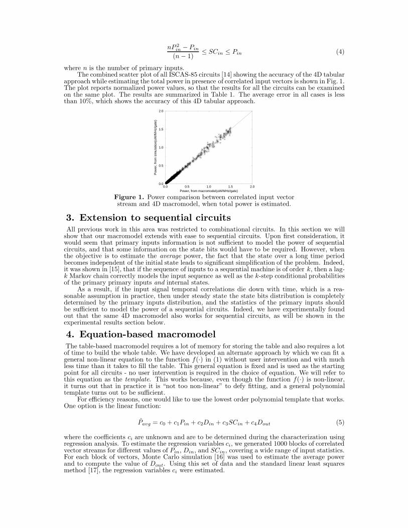
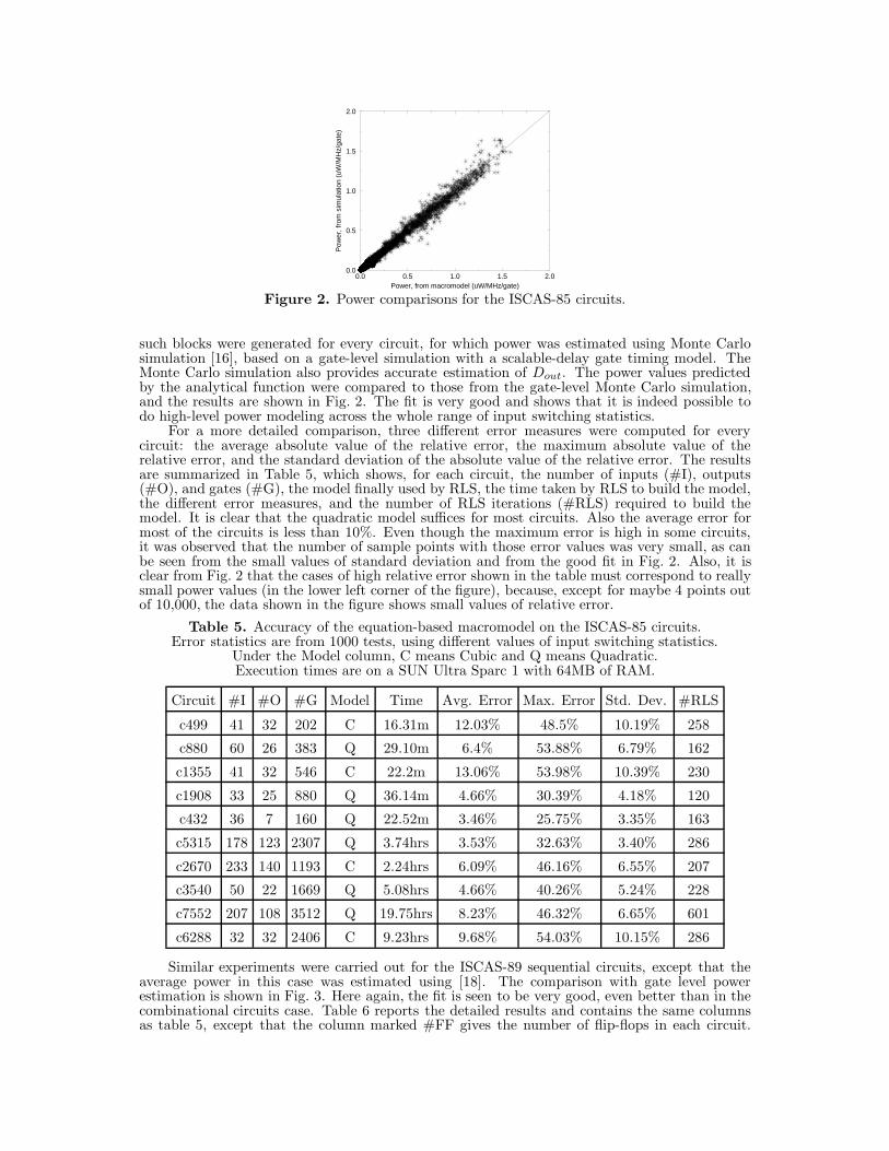
Figure 2. Power comparisons for the ISCAS-85 circuits.

such blocks were generated for every circuit, for which power was estimated using Monte Carlosimulation [16], based on a gate-level simulation with a scalable-delay gate timing model. TheMonte Carlo simulation also provides accurate estimation of Dout. The power values predictedby the analytical function were compared to those from the gate-level Monte Carlo simulation,and the results are shown in Fig. 2. The fit is very good and shows that it is indeed possible todo high-level power modeling across the whole range of input switching statistics.

For a more detailed comparison, three different error measures were computed for everycircuit: the average absolute value of the relative error, the maximum absolute value of therelative error, and the standard deviation of the absolute value of the relative error. The resultsare summarized in Table 5, which shows, for each circuit, the number of inputs (#I), outputs(#O), and gates (#G), the model finally used by RLS, the time taken by RLS to build the model,the different error measures, and the number of RLS iterations (#RLS) required to build themodel. It is clear that the quadratic model suffices for most circuits. Also the average error formost of the circuits is less than 10%. Even though the maximum error is high in some circuits,it was observed that the number of sample points with those error values was very small, as canbe seen from the small values of standard deviation and from the good fit in Fig. 2. Also, it isclear from Fig. 2 that the cases of high relative error shown in the table must correspond to reallysmall power values (in the lower left corner of the figure), because, except for maybe 4 points outof 10,000, the data shown in the figure shows small values of relative error.

Table 5. Accuracy of the equation-based macromodel on the ISCAS-85 circuits.Error statistics are from 1000 tests, using different values of input switching statistics.

Under the Model column, C means Cubic and Q means Quadratic.Execution times are on a SUN Ultra Sparc 1 with 64MB of RAM.

Circuit #I #O #G Model Time Avg. Error Max. Error Std. Dev. #RLS

c499 41 32 202 C 16.31m 12.03% 48.5% 10.19% 258

c880 60 26 383 Q 29.10m 6.4% 53.88% 6.79% 162

c1355 41 32 546 C 22.2m 13.06% 53.98% 10.39% 230

c1908 33 25 880 Q 36.14m 4.66% 30.39% 4.18% 120

c432 36 7 160 Q 22.52m 3.46% 25.75% 3.35% 163

c5315 178 123 2307 Q 3.74hrs 3.53% 32.63% 3.40% 286

c2670 233 140 1193 C 2.24hrs 6.09% 46.16% 6.55% 207

c3540 50 22 1669 Q 5.08hrs 4.66% 40.26% 5.24% 228

c7552 207 108 3512 Q 19.75hrs 8.23% 46.32% 6.65% 601

c6288 32 32 2406 C 9.23hrs 9.68% 54.03% 10.15% 286

Similar experiments were carried out for the ISCAS-89 sequential circuits, except that theaverage power in this case was estimated using [18]. The comparison with gate level powerestimation is shown in Fig. 3. Here again, the fit is seen to be very good, even better than in thecombinational circuits case. Table 6 reports the detailed results and contains the same columnsas table 5, except that the column marked #FF gives the number of flip-flops in each circuit.

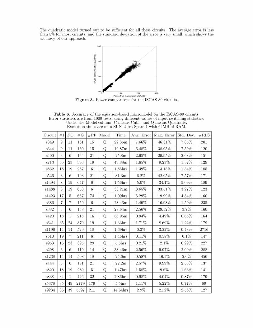
The quadratic model turned out to be sufficient for all these circuits. The average error is lessthan 5% for most circuits, and the standard deviation of the error is very small, which shows theaccuracy of our approach.

0.0 10.0 20.0 30.0Power, from macromodel (uW/MHz)

0.0

10.0

20.0

30.0

Pow

er, f

rom

sim

ulat

ion

(uW

/MH

z)

Figure 3. Power comparisons for the ISCAS-89 circuits.

Table 6. Accuracy of the equation-based macromodel on the ISCAS-89 circuits.Error statistics are from 1000 tests, using different values of input switching statistics.

Under the Model column, C means Cubic and Q means Quadratic.Execution times are on a SUN Ultra Sparc 1 with 64MB of RAM.

Circuit #I #O #G #FF Model Time Avg. Error Max. Error Std. Dev. #RLS

s349 9 11 161 15 Q 22.36m 7.66% 46.31% 7.85% 201

s344 9 11 160 15 Q 19.87m 6.48% 38.95% 7.59% 120

s400 3 6 164 21 Q 25.8m 2.65% 29.95% 2.68% 151

s713 35 23 393 19 Q 49.88m 1.65% 9.23% 1.52% 129

s832 18 19 287 6 Q 1.85hrs 1.39% 13.15% 1.54% 185

s526 3 6 193 21 Q 31.3m 6.2% 42.95% 7.57% 171

s1494 8 19 647 6 Q 1.56hrs 5.0% 34.1% 5.09% 189

s1488 8 19 653 6 Q 33.21m 3.65% 33.51% 3.27% 123

s1423 17 5 657 74 Q 1.09hrs 5.29% 19.99% 4.54% 160

s386 7 7 159 6 Q 28.43m 1.49% 16.98% 1.59% 235

s382 3 6 158 21 Q 28.64m 2.56% 29.52% 3.7% 160

s420 18 1 218 16 Q 56.96m 0.94% 4.49% 0.68% 164

s641 35 24 379 19 Q 1.33hrs 1.71% 8.69% 1.22% 179

s1196 14 14 529 18 Q 1.69hrs 0.3% 3.22% 0.43% 2716

s510 19 7 211 6 Q 1.45hrs 0.11% 0.58% 0.1% 147

s953 16 23 395 29 Q 5.5hrs 0.21% 2.1% 0.29% 227

s298 3 6 119 14 Q 38.46m 2.56% 9.97% 2.09% 288

s1238 14 14 508 18 Q 25.6m 0.58% 16.5% 2.0% 456

s444 3 6 181 21 Q 22.2m 2.57% 9.99% 2.55% 137

s820 18 19 289 5 Q 1.47hrs 1.58% 9.6% 1.63% 141

s838 34 1 446 32 Q 2.86hrs 0.98% 4.04% 0.87% 179

s5378 35 49 2779 179 Q 5.5hrs 1.11% 5.22% 0.77% 89

s9234 36 39 5597 211 Q 14.64hrs 2.9% 21.2% 2.56% 127

7. ConclusionSince gate-level power estimation can be time-consuming and because power estimation from a

high level of abstraction is desirable so as to reduce design time and cost, we have proposed anequation-based power macromodeling approach for combinational and sequential circuits. Ourmacromodel consists of an analytical function with four variables: average input signal probability,average input switching activity, average input spatial correlation coefficient, and average output(zero-delay) switching activity. We also presented a Recursive Least Squares (RLS) algorithm bywhich such an analytical expression can be generated. The proposed model works for all possiblesignal switching statistics and no user intervention is needed for the model characterization. Theonly thing that the user has to specify is how much accuracy is desired. The macromodel hasbeen built and tested for many combinational and sequential benchmark circuits.

References[1] F. N. Najm, “A survey of power estimation techniques in VLSI circuits,” IEEE Transactions on

VLSI Systems, pp. 446-455, Dec. 1994.

[2] P. Landman, High-level power estimation, “International Symposium on Low Power Electronics andDesign,” pp. 29–35, Monterey, CA, August 12–14, 1996.

[3] M. Nemani and F. N. Najm, “Towards a High-Level Power Estimation Capability,” IEEE Transac-tions on CAD, vol. 15 pp. 588-598, June 1996.

[4] D. Marculescu, R. Marculescu and M. Pedram, “Information Theoretic Measures of Energy Con-sumption at Register Transfer Level,” ACM/IEEE International Symposium on Low Power Design,pp. 87-92, April 1995.

[5] S. R. Powell and P. M. Chau, “ Estimating Power Dissipation of VLSI signal Processing Chips: ThePFA technique,” VLSI Signal Processing IV, pp. 250-259, 1990.

[6] P. E. Landman and J. M. Rabaey, “Architectural Power Analysis: The Dual Bit Type Method,”IEEE Transactions on VLSI, vol. 3 pp. 173-187 June 1995.

[7] H. Mehta, R. M. Owens and M. J. Irwin, “Energy Characterization based on Clustering,” 33rdACM/IEEE Design Automation Conference, pp. 702-707, June 1996.

[8] A. Raghunathan, S. Dey and N. K. Jha, “Register-Transfer Level Estimation Techniques for Switch-ing Activity and Power Consumption,” IEEE International Conference on Computer-Aided Design,pp. 158-165, November 1996.

[9] Q. Qiu, Q. Wu, Chih-S. Ding, and M. Pedram, “Cycle-accurate macro-models for RT-level poweranalysis,” Proc. International Symposium on Low Power Electronics and Design, pp. 125–130, 1997.

[10] S. Gupta and F. N. Najm,“Power Macromodeling for High Level Power Estimation,”34th ACM/IEEEDesign Automation Conference, pp. 365-370, June 1997.

[11] S. Gupta and F. N. Najm, “Power Macromodeling for High Level Power Estimation,” University ofIllinois, Coordinated Science Laboratory, Report #UILU-ENG-97-2229, September 1997.

[12] F. N. Najm, “Transition Density: A New Measure of Activity in Digital Circuits,” IEEE Trans. onCAD, vol. 12, pp. 310-323, Feb. 1993.

[13] S. Gupta and F. N. Najm, “Power Macromodeling for High Level Power Estimation,” Submitted toIEEE Transactions on VLSI, 1997.

[14] F. Brglez and H. Fujiwara, “A neutral netlist of 10 combinational benchmark circuits and a targettranslator in Fortran,” IEEE International Symposium on Circuits and Systems, pp. 695-698, June1985.

[15] D. Marculescu, R. Marculescu, and M. Pedram, “Sequence Compaction for Probabilistic Analysis ofFinite-State Machines,” 34th ACM/IEEE Design Automation Conference, pp. 12-15, June 1997.

[16] M. Xakellis and F. N. Najm, “Statistical Estimation of the Switching Activity in Digital Circuits,”31st ACM/IEEE Design Automation Conference, pp. 728-733, June 1994.

[17] G. Seber, Linear Regression Analysis. New York: John Wiley & Sons, 1977.

[18] J. Kozhaya and F. N. Najm, “Accurate power estimation for large sequential circuits,” IEEE Inter-national Conference on Computer-Aided Design, pp. 448-493, November 1997.

[19] L. Ljung, System Identification: theory for the user. Engelwood Cliffs, NJ: Prentice Hall, 1987.

[20] I. R. Miller, J. E. Freund, and R. Johnson, Probability and Statistics for Engineers, 4th Ed., Engle-wood Cliffs, NJ: Prentice-Hall Inc., 1990, pp. 210-211.