analytical quality control in shipping operation using six ... · analytical quality control in...
TRANSCRIPT

Analytical Quality Control in Shipping Operation
Using Six Sigma Principles
A Thesis Submitted in Partial Fulfilment of the
Requirements of Liverpool John Moores University for the
Degree of Doctor of Philosophy
Zhuohua Qu
March 2015

i
Acknowledgements
The completion of this research would not have been accomplished without the help
and support from many individuals and organizations.
I could not express enough appreciation to my supervisors Professor Ian Jenkinson
and Professor Jin Wang for all their continuous support, invaluable guidance and
encouragement throughout my PhD journey. I am also thankful to Liverpool John
Moors University (LJMU) for its generous patronage.
I would like to express my gratitude to all the industrial collaborators for their most
helpful support in this research which has made it possible to achieve the research
goal.
I am indebted to my family members for their love, patience and encouragement
during my research. For my daughter “Sophie”, thank you for giving me so much
happiness during this long and sometimes, difficult, journey. Finally, my deepest
gratitude goes to my loving and supportive husband, Zaili Yang. It is your
encouragement and support, especially when time went rough, that has made this
thesis possible. My heartfelt thanks!

ii
Abstract
A large number of benefits achieved through the successful implementation of Six
Sigma programmes in different industries have been documented. However, very
little research has been conducted on their applications in the shipping sector,
especially in the Onshore Service Functions (OSFs) of shipping companies.
Literature shows that heavy human involvement in the service industries such as
shipping leads to a high volume of uncertainties which are difficult to be correctly
and effectively measured or managed by simply using the traditional data analysis
and statistical methods in Six Sigma. The aim of this study is to develop new
quantitative analytical methodologies to enable the application and implementation
of Six Sigma to improve the service quality of OSFs in shipping companies.
Intensive investigations on the feasibility and effectiveness of the developed new
methods and models through case studies in world leading container ship lines and
shipping management companies have been carried out to ensure the achievement of
the aim.
This study firstly reviews the evolvement of quality control and some typical
methods in the area, the development of Six Sigma, its tools and current applications,
especially in the service industries. It is followed by a new framework of the Six
Sigma implementation in the OSFs of shipping companies which is supported by a
few real process excellence projects carried out in a world-leading ship line. In the
process of the framework development, various issues and challenges appear largely
due to the existence of uncertainties in data such as ambiguity and incompleteness
caused by extensive subjective judgements. Advanced methods and models are
developed to tackle the above challenges as well as complement the traditional Six
Sigma tools so that the new Six Sigma methodologies can be confidently applied in
situations where uncertainties in data exist at different levels.
A new fuzzy Technique for Order Preference by Similarity to an Ideal Solution

iii
(TOPSIS) method is developed by combining the traditional TOPSIS, fuzzy numbers
and interval approximation sets to facilitate the effective selection of Six Sigma
projects and achieve the optimal use of resources towards the company objectives. A
revised Failure Mode and Effects Analysis (FMEA) model is proposed in the
“Analyse” step in Six Sigma to improve the capability of classical FMEA in failure
identification in service industries. The new FMEA model uses the Analytical
Hierarchy Process (AHP) and Fuzzy Bayesian Reasoning (FBR) approaches to
increase the accuracy of failure identification while not compromising the easiness
and visibility of the Risk Priority Number (RPN) method. Decision Making Trial and
Evaluation Laboratory (DEMATEL) and Analytical Network Process (ANP)
methods are incorporated with Fuzzy logic and Evidential Reasoning (ER), for the
very first time to generate a Key Performance Indicators (KPIs) management method
where the weights of indicators are rationally assigned by considering the
interdependency among the indicators. Incomplete and fuzzy evaluations of the KPIs
are synthesised in a rational way to achieve a compatible and comparable result.
It is concluded that the newly developed Six Sigma framework together with its
supporting quantitative analytical models has made significant contribution to
facilitate the quality control and process improvement in shipping companies. It has
been strongly evidenced by the success of the applications of the new models in real
cases. The financial gains and continuous benefits produced in the investigated
shipping companies have attracted a wider range of interests from different service
industries. It is therefore believed that this work will have a high potential to be
tailored for a wide range of applications across sectors and industries when the
uncertainties in data exceed the ability that the classical Six Sigma tools and methods
possess.
iv
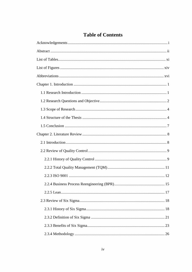
Table of Contents
Acknowledgements ....................................................................................................... i
Abstract ........................................................................................................................ ii
List of Tables............................................................................................................... xi
List of Figures ........................................................................................................... xiv
Abbreviations ............................................................................................................ xvi
Chapter 1. Introduction ................................................................................................ 1
1.1 Research Introduction ........................................................................................ 1
1.2 Research Questions and Objective ..................................................................... 2
1.3 Scope of Research .............................................................................................. 4
1.4 Structure of the Thesis ....................................................................................... 4
1.5 Conclusion ......................................................................................................... 7
Chapter 2. Literature Review ....................................................................................... 8
2.1 Introduction ........................................................................................................ 8
2.2 Review of Quality Control ................................................................................. 9
2.2.1 History of Quality Control .......................................................................... 9
2.2.2 Total Quality Management (TQM) ........................................................... 11
2.2.3 ISO 9001 ................................................................................................... 12
2.2.4 Business Process Reengineering (BPR) .................................................... 15
2.2.5 Lean ........................................................................................................... 17
2.3 Review of Six Sigma ........................................................................................ 18
2.3.1 History of Six Sigma ................................................................................. 18
2.3.2 Definition of Six Sigma ............................................................................ 21
2.3.3 Benefits of Six Sigma................................................................................ 23
2.3.4 Methodology ............................................................................................. 26

v
2.3.5 Critical Success Factors (CSFs) ................................................................ 26
2.4 Tools in Six Sigma ........................................................................................... 33
2.4.1 Project Charter .......................................................................................... 33
2.4.2 Critical to Quality (CTQ) Tree .................................................................. 35
2.4.3 Process Mapping ....................................................................................... 36
2.4.4 Measurement System Analysis (MSA) ..................................................... 38
2.4.5 Control Chart ............................................................................................. 42
2.4.6 Process Capability Analysis (PCA) .......................................................... 45
2.4.7 Cause and Effect (C&E) Matrix ................................................................ 47
2.4.8 Failure Mode and Effects Analysis (FMEA) ............................................ 49
2.4.9 Pareto Charts ............................................................................................. 51
2.5 Six Sigma in the Service Industries ................................................................. 53
2.6 Decision Making under Uncertainty ................................................................ 55
2.7 Discussion ........................................................................................................ 62
Chapter 3. A Modified Six Sigma Methodology for OSFs of Shipping Companies . 63
3.1 Introduction ...................................................................................................... 63
3.2 The Needs of Six Sigma in the OSFs of Shipping Companies ........................ 63
3.3 A Modified Six Sigma Methodology ............................................................... 65
3.3.1 Top Management Support / Involvement ................................................. 65
3.3.2 Prepare....................................................................................................... 66
3.3.3 DMAIC ..................................................................................................... 69
3.3.4 Recognize Contribution and Success ........................................................ 73
3.4 Implementation of Six Sigma in OSFs of Shipping Companies – a Real Case
Study of a World Leading Shipping Line .............................................................. 73
3.4.1 Prepare....................................................................................................... 74

vi
3.4.2 DMAIC ..................................................................................................... 75
3.4.3 Recognize Contribution and Success ........................................................ 82
3.5 Issues Encountered and Lessons Learned ........................................................ 82
3.5.1 Effective Tools in Project Selection .......................................................... 82
3.5.2 Qualitative Data Analysis ......................................................................... 83
3.5.3 KPIs Management ..................................................................................... 83
3.5.4 Training ..................................................................................................... 84
3.5.5 Resources Availability .............................................................................. 84
3.5.6 Effective Communication ......................................................................... 84
3.6 Conclusion ....................................................................................................... 85
Chapter 4. Project Selection Using Fuzzy TOPSIS ................................................... 87
4.1 Introduction ...................................................................................................... 87
4.2 Literature on Six Sigma Project Selection Methodology ................................. 89
4.3 Fuzzy TOPSIS Methods ................................................................................... 91
4.4 The New Approximate TOPSIS with Belief Structures .................................. 93
4.4.1 Identify Alternatives and Criteria to Establish the Decision Making Matrix
Format with the Presentation of All Alternatives and Criteria .......................... 95
4.4.2 Evaluate the Ratings of Alternatives with Respect to Each Criterion and
the Importance of the Criteria, 𝒘𝒋 ...................................................................... 95
4.4.3 Transform Ratings of Alternatives to TPFN ............................................. 97
4.4.4 Aggregate the Fuzzy Ratings and Weights from Multiple Decision Makers
............................................................................................................................ 99
4.4.5 Normalise the Fuzzy Decision Rating Matrix ........................................... 99
4.4.6 Constructed Weighted Normalized Fuzzy Decision Matrix ................... 100
4.4.7 Determine FPIS and FNIS ...................................................................... 100
4.4.8 Calculate the Distances of Each Alternative from FPIS and FNIS ......... 101

vii
4.4.9 Calculate the Distance Closeness Coefficient of Each Alternative ........ 101
4.4.10 Rank the Alternatives According to their Closeness Coefficients ........ 101
4.4.11 Validation using Benchmarking Techniques ........................................ 102
4.5 Six Sigma Project Selections Using the Revised TOPSIS ............................. 102
4.5.1 Identify Alternatives, Criteria and the Corresponding Data Nature to
Establish the Decision Making Matrix Format ................................................ 102
4.5.2 Evaluate the Ratings of Alternatives with Respect to Each Criterion and
the Importance of the Criteria, 𝒘𝒋 .................................................................... 104
4.5.3 Transform Ratings of Alternatives to TPFN and Aggregate the Fuzzy
Ratings from Multiple Decision Makers .......................................................... 105
4.5.4 Normalise the Fuzzy Decision Rating Matrix ......................................... 107
4.5.5 Constructed Weighted Normalized Fuzzy Decision Matrix ................... 107
4.5.1 Determine FPIS and FNIS ...................................................................... 107
4.5.2 Calculate the Distances of Each Alternative from FPIS and FNIS ......... 110
4.5.3 Calculate the Distance Closeness Coefficient of Each Alternative ........ 110
4.5.4 Validation using Benchmarking Techniques .......................................... 111
4.6 Discussion and Conclusion ............................................................................ 112
Chapter 5. Revised FMEA Model to Facilitate Six Sigma in Shipping Companies 116
5.1 Introduction .................................................................................................... 116
5.2 Literature Review ........................................................................................... 118
5.2.1 Use FMEA in Six Sigma ......................................................................... 118
5.2.2 Traditional FMEA ................................................................................... 119
5.2.3 AHP ......................................................................................................... 121
5.2.4 Fuzzy Bayesian Reasoning ..................................................................... 121
5.3 A Revised FMEA Methodology using AHP and FRB .................................. 123
5.3.1 Assessing the Weights of the Three Criteria in FMEA (S, O, D) Using

viii
AHP Method .................................................................................................... 123
5.3.2 Establishing a FRB with a Rational Belief Structure .............................. 126
5.3.3 Assessment of Failures Using Fuzzy Belief Structures .......................... 127
5.3.4 Rule Aggregation with the Weights of FMEA Criteria Using Bayesian
Reasoning ......................................................................................................... 131
5.3.5 Failure Ranking ....................................................................................... 133
5.3.6 Validation ................................................................................................ 134
5.4 A Case Analysis of Accounting Management in Shipping Lines .................. 134
5.4.1 Establish a Pair-wise Comparison Decision Matrix and Calculate the
Weight for Each Criterion ................................................................................ 135
5.4.2 Rule Establishment with a Rational Belief Structure .............................. 136
5.4.3 Use Subjective Judgements to Estimate the Failure Modes ................... 137
5.4.4 Conduct the Risk Inference ..................................................................... 139
5.4.5 Prioritization of the Failures.................................................................... 140
5.4.6 Validation of the Result .......................................................................... 141
5.5 Conclusion ..................................................................................................... 144
Chapter 6. Evaluating KPIs in Shipping Management by Using DEMATEL, ANP
and ER ...................................................................................................................... 146
6.1 Introduction .................................................................................................... 146
6.2 Literature Review ........................................................................................... 148
6.2.1 KPIs in the Shipping Industry ................................................................. 148
6.2.2 DEMATEL .............................................................................................. 149
6.2.3 ANP ......................................................................................................... 150
6.2.4 Fuzzy Logic and Evidential Reasoning (ER) Algorithm ........................ 151
6.3 KPIs Management in the Shipping Industry by Using DEMATL, ANP and
FER ...................................................................................................................... 152

ix
6.3.1 Identify KPIs and PIs to Build a KPI Tree .............................................. 153
6.3.2 Assess the Interdependencies of the Top Level Indicators using
DEMATEL ....................................................................................................... 155
6.3.3 Obtain Lower Level Indicator Weights by using the ANP Method........ 158
6.3.4 Set Criterion Grade and Collect Data for the Lowest Level Indicators .. 161
6.3.5 Transform the Evaluation from the Lowest Level to Top Level Grades 162
6.3.6 Synthesise Indicators from the Lowest Level PIs to Top Level KPIs by
using an ER Algorithm .................................................................................... 163
6.4 A Case Study of KPI Tree Management in a Shipping Management Company
.............................................................................................................................. 167
6.4.1 Assess the Interdependencies of the KPIs Using DEMATEL ................ 168
6.4.2 Obtain the Weights for the Lower Level Indicators by using the ANP
method .............................................................................................................. 172
6.4.3 Set Criterion Grades and Collect Data for the Lowest Level Indicators . 180
6.4.4 Transform the Evaluation and Synthesis Indicators from the Lowest Level
to Top Level by using an ER Algorithm .......................................................... 181
6.5 Conclusion ..................................................................................................... 188
Chapter 7. Discussion and Conclusion .................................................................... 191
7.1 Introduction .................................................................................................... 191
7.2 Key Findings and Contributions from the Research ...................................... 192
7.2.1 Findings on the Issues regarding the Implementation of Six Sigma in
OSFs of Shipping Companies .......................................................................... 192
7.2.2 Findings and Contributions of the New Fuzzy TOPSIS for Project
Selection ........................................................................................................... 193
7.2.3 Findings and Contributions regarding the Revised FMEA Model ......... 194
7.2.4 Findings and Contributions regarding the KPIs Management Method .. 195

x
7.3 Limitations of the Research and Suggestions for Future Research ............... 196
7.3.1 Limitations of the Research .................................................................... 196
7.3.2 Suggestions for Future Research ............................................................. 197
References ................................................................................................................ 200
Appendices ............................................................................................................... 217

xi
List of Tables
Table 2.1 History of statistical process control .......................................................... 10
Table 2.2 Six Sigma vs. TQM .................................................................................... 13
Table 2.3 BPR vs. Six Sigma ..................................................................................... 16
Table 2.4 Lean vs. Six Sigma..................................................................................... 19
Table 2.5 Some quality control methods with a brief description ............................. 19
Table 2.6 Simplified sigma levels .............................................................................. 22
Table 2.7 Reported benefits and savings through Six Sigma in the manufacturing
sector .......................................................................................................................... 24
Table 2.8 Benefits of Six Sigma in both manufacturing and service organisations .. 24
Table 2.9 CSFs for successful implementation of Six Sigma .................................... 28
Table 2.10 Common causes and special causes ......................................................... 43
Table 2.11 PCIs – Cp and Cpk ................................................................................... 46
Table 2.12 Relation scores for C&E matrix ............................................................... 48
Table 2.13 Explanation of Severity, Occurrence and Detection in FMEA ................ 50
Table 2.14 FMEA applications in Six Sigma phases ................................................. 50
Table 2.15 FMEA form .............................................................................................. 51
Table 2.16 Useful tools in Six Sigma projects ........................................................... 52
Table 2.17 Differences between service and manufacturing industries ..................... 55
Table 3.1 Six Sigma belt system ................................................................................ 68
Table 3.2 Key characteristics associated with internal versus external training
(Kubiak, 2012) ........................................................................................................... 69
Table 3.3 Example of a measurement plan ................................................................ 71
Table 3.4 An example template of control plan ......................................................... 73
Table 3.5 C&E matrix for non-recovered wasted journeys – top ranked inputs........ 78
Table 3.6 FMEA for non-recovered wasted journey ................................................. 79
Table 3.7 Data collection plan ................................................................................... 79
Table 3.8 Control plan................................................................................................ 81
Table 4.1 Linguistic variables for the ratings alternatives ......................................... 96
Table 4.2 Linguistic variables for the importance weight of each criterion .............. 97

xii
Table 4.3 Six Sigma project selection criteria overview.......................................... 103
Table 4.4 The importance weight of the criteria given by decision makers ............ 105
Table 4.5 The rating of alternatives by decision makers under all criteria .............. 105
Table 4.6 The importance weight of the criteria in TPFN ....................................... 108
Table 4.7 The rating of alternatives by decision makers under all criteria in TPFN 108
Table 4.8 Normalized fuzzy decision matrix ........................................................... 109
Table 4.9 Weighted normalized fuzzy decision matrix .......................................... 109
Table 4.10 Distances of each alternative from FPIS and FNIS .............................. 110
Table 4.11 The possible best rating of alternatives by decision makers under all
criteria ...................................................................................................................... 113
Table 4.12 The possible worst rating of alternatives by decision makers under all
criteria ...................................................................................................................... 114
Table 4.13 Normalized possible best rating matrix ................................................. 115
Table 4.14 Normalized possible worst rating matrix ............................................... 115
Table 5.1 Judgement scores in AHP (Saaty, 1980) .................................................. 124
Table 5.2 Random index (RI) for the factors used in the decision making process. 126
Table 5.3 FRB with belief structures and weights of criteria in FMEA .................. 127
Table 5.4 Fuzzy ratings for linguistic terms. ........................................................... 129
Table 5.5 The Conditional Probability Table of NR ................................................. 132
Table 5.6 Failure modes identified........................................................................... 136
Table 5.7 Comparison matrix for FMEA criteria..................................................... 136
Table 5.8 Sample of a new FMEA rule base with a rational belief structure .......... 137
Table 5.9 Ratings for S, O and D. ............................................................................ 138
Table 5.10 Expert subjective input for S, O and D .................................................. 138
Table 5.11 Belief degrees transformed from expert evaluations ............................. 138
Table 5.12 RI values for the failure modes identified .............................................. 141
Table 6.1 KPI tree structure ..................................................................................... 168
Table 6.2 Evaluation table for the degree of influences........................................... 169
Table 6.3 Degree of importance through DEMATEL ............................................. 171
Table 6.4 Pairwise comparison table for the evaluation of influences .................... 173
Table 6.5 Evaluations for the level of influences among C1, C2 and C3 in regards to

xiii
indicator A1 .............................................................................................................. 173
Table 6.6 Unweighted supermatrix .......................................................................... 176
Table 6.7 Cluster weight matrix ............................................................................... 177
Table 6.8 Weighted supermatrix .............................................................................. 178
Table 6.9 Limiting supermaterix .............................................................................. 179
Table 6.10 Weights of lowest level indicators ......................................................... 180
Table 6.11 Indicator evaluations and grades associated with linguistic terms ........ 182
Table 6.12 Belief degrees transformed from the evaluations form all indicators .... 190
xiv
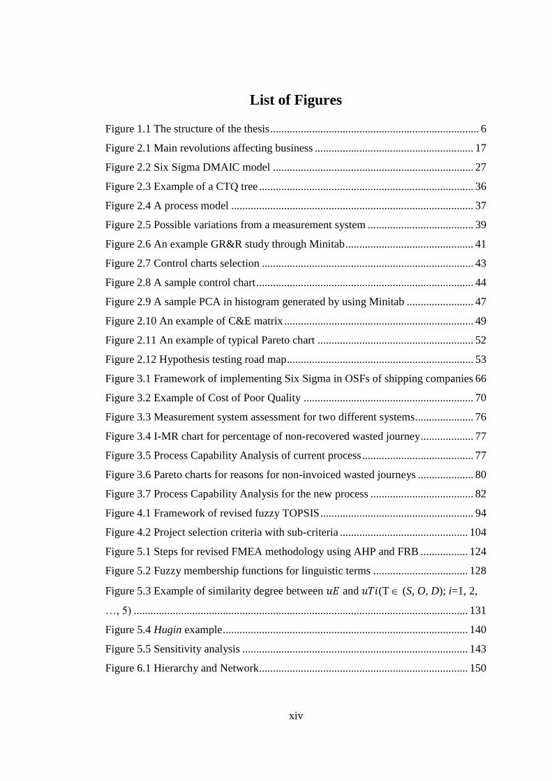
List of Figures
Figure 1.1 The structure of the thesis ........................................................................... 6
Figure 2.1 Main revolutions affecting business ......................................................... 17
Figure 2.2 Six Sigma DMAIC model ........................................................................ 27
Figure 2.3 Example of a CTQ tree ............................................................................. 36
Figure 2.4 A process model ....................................................................................... 37
Figure 2.5 Possible variations from a measurement system ...................................... 39
Figure 2.6 An example GR&R study through Minitab .............................................. 41
Figure 2.7 Control charts selection ............................................................................ 43
Figure 2.8 A sample control chart .............................................................................. 44
Figure 2.9 A sample PCA in histogram generated by using Minitab ........................ 47
Figure 2.10 An example of C&E matrix .................................................................... 49
Figure 2.11 An example of typical Pareto chart ........................................................ 52
Figure 2.12 Hypothesis testing road map ................................................................... 53
Figure 3.1 Framework of implementing Six Sigma in OSFs of shipping companies 66
Figure 3.2 Example of Cost of Poor Quality ............................................................. 70
Figure 3.3 Measurement system assessment for two different systems..................... 76
Figure 3.4 I-MR chart for percentage of non-recovered wasted journey ................... 77
Figure 3.5 Process Capability Analysis of current process ........................................ 77
Figure 3.6 Pareto charts for reasons for non-invoiced wasted journeys .................... 80
Figure 3.7 Process Capability Analysis for the new process ..................................... 82
Figure 4.1 Framework of revised fuzzy TOPSIS ....................................................... 94
Figure 4.2 Project selection criteria with sub-criteria .............................................. 104
Figure 5.1 Steps for revised FMEA methodology using AHP and FRB ................. 124
Figure 5.2 Fuzzy membership functions for linguistic terms .................................. 128
Figure 5.3 Example of similarity degree between 𝑢𝐸 and 𝑢𝑇𝑖(T (S, O, D); i=1, 2,
…, 5) ........................................................................................................................ 131
Figure 5.4 Hugin example ........................................................................................ 140
Figure 5.5 Sensitivity analysis ................................................................................. 143
Figure 6.1 Hierarchy and Network........................................................................... 150

xv
Figure 6.2 Proposed framework for KPI management ............................................ 154
Figure 6.3 i, j block of a supermatrix in ANP .......................................................... 160
Figure 6.4 impact relations-map from DEMATEL ................................................. 172
Figure 6.5 Relationship diagram created in “Super decisions” software ................. 175
Figure 6.6 Ranking for the company overall performance over four-month period 187
Figure 6.7 Comparison of KPIs over four-month period ......................................... 188

xvi
Abbreviations
AHP Analytical Hierarchy Process
ANFIS Adaptive Neural Fuzzy Inference Systems
ANP Analytical Network Process
ANSI American National Standards Institute
BB Black Belt
BN Bayesian Networks
BOA Bank of America
BPR Business process re-engineering
BSI British Standards Institute
C&E Matrix Cause and Effect Matrix
CEO Chief Executive Officer
COPQ Cost Of Poor Quality
CPT Conditional Probability Table
CSFs Critical Success Factors
CTQ Critical To Quality
CWQT CompanyWide Quality Control
DEA Data Envelopment Analysis
DEMATEL Decision Making Trial and Evaluation Laboratory
DFSS Design for Six Sigma
DMAIC Define, Measure, Analyse, Improve, and Control
DOE Design Of Experiment
DPMO Defects Per Million Opportunities
EFA Exploratory Factor Analysis
ER Evidential Reasoning
FAHP Fuzzy Analytical Hierarchy Process
FBR Fuzzy Bayesian Reasoning
FER Fuzzy Evidential Reasoning
FMEA Failure Mode Effects Analysis
FMECA Failure Mode, Effects and Criticality Analysis
FNIS Fuzzy Negative Ideal Solution
FPIS Fuzzy Positive Ideal Solution
FuRBaR Fuzzy Rule-Based Bayesian Reasoning
GB Green Belt
GE General Electric
GR&R Gage Repeatability and Reproducibility
ID Influence Diagram
ISM International Safety Management
ISO International Organization for Standardization
KPIs Key Performance Indicators
LCL Lower Control Limit

xvii
LSL Lower Specification Limit
MBB Master Black Belt
MCDM Multiple Criteria Decision Making
NIS Negative Ideal Solution
OSFs Onshore Service Functions
PBR Possible Best Rating
PCA Process Capability Analysis
PDCA Plan-Do-Check-Act
PDM Project Desirability Matrix
PIS Positive Ideal Solution
PMBOK Project Management Body of Knowledge
PWR Possible Worst Rating
QMS Quality Management System
RIMER
Rule based Inference Methodology using the Evidential
Reasoning algorithm
RPN Risk Priority Number
SPC Statistical Process Control
SWOT Strength, Weakness, Opportunities and Threats
TOPSIS
Technique for Order Preference by Similarity to an Ideal
Solution
TPFN Trapezoidal Fuzzy Number
TQM Total Quality Management
UCL Upper Control Limit
USL Upper Specification Limit
VOC Voice Of Customer
FRB Fuzzy Rule Base
IDS Intelligent Decision System

Chapter 1. Introduction
1
Chapter 1. Introduction
1.1 Research Introduction
The past decades have witnessed increasing competition in the global market and
companies are operating in an ever increasing competitive environment. In order to
maintain their competitiveness, companies are paying increasing attention to enhance
their performances in order to retain customers, especially under the current
economic environment. Profitability alone is not sufficient to discriminate
excellence. The shipping industry carries around 90% of world trade (I.C.S., 2013)
and plays an important role in global economic development and world prosperity.
Due to the fact that shipping is a capital intensive and highly dangerous industry,
quality control in ship building, maintenance and operations has always attracted the
attention of stakeholders. Thus many shipping companies have adopted quality
management systems (QMS) to ensure and improve safety in ship operations,
including: Total Quality Management (TQM), ISO quality management systems, and
the International Safety Management (ISM) code. However, shipping includes not
only the carriage of goods by sea, but also the associated services, such as customer
support, finance and accounting. Globalisation has accelerated the exposure of
companies to competition and shipping alone could hardly achieve sustainable
competitive differentiation. As a result, companies are increasingly investigating the
ways of improving the associated services provided by their onshore service
functions (OSFs) to better meet customer requirements and reduce unnecessary costs.
Six Sigma is a business strategy that uses a well-structured methodology to improve
process performance and eliminate defects in order to achieve continuous
improvement within the business process. Having seen the remarkable improvements
resulting from the Six Sigma implementation in General Electric (GE), businesses in
many sectors are joining the Six Sigma brand wagon, including construction,

Chapter 1. Introduction
2
healthcare, banking and many more. Six Sigma has been successfully implemented
for over 20 years across different industries with significant improvements achieved.
It has been used to continuously improve business processes, reduce costs and
improve customer satisfaction while maintaining profitability. However, most of the
studies of the implementation of Six Sigma in service industries have focused mainly
on some particular sectors such as supply chain management, banking and health
care. Limited studies of investigating the applications of Six Sigma in the shipping
related industries have been found in port security studies (Ung et al., 2007),
maritime training and education (Er and Gurel, 2005) and container terminal
operations (Nooramin et al., 2011). No studies are found in the literature on the
application of Six Sigma in OSFs of shipping companies. Research has also revealed
several unique challenges in applying Six Sigma in OSFs of shipping companies.
These include invisible work processes, lack of qualified information and vast
differentiation among customer needs. As a result there is a significant research gap
to be fulfilled.
This chapter gives a brief introduction and essentially “sets the scene” for the thesis
by: explaining the research objectives, primary and subsidiary; presenting the
proposed methodology and describing the layout and scope of the thesis.
1.2 Research Questions and Objective
Six Sigma works best when it uses hard data as the foundation for process
improvement. It is the reason why one of the general interpretations of this
programme is that it is heavy on statistics. However, Chakrabarty and Chuan
(2009)’s study has revealed that over 72% of service companies that responded to the
survey consider data collecting is a barrier in Six Sigma implementation. In OSFs,
due to the fact of undefined processes, interviews and brainstorming are the tools
frequently used which often result in a large number of uncertainties due to the
presentation of qualitative and ambiguous data. It therefore becomes difficult to

Chapter 1. Introduction
3
define quality and apply some of the existing statistical tools. Traditional use of
quantitative data in analysis turns into a challenge during Six Sigma applications.
Lack of qualified data can lead to difficulties in many phases of the implementation
process which may lead to ineffective improvement actions.
The existing literature on Six Sigma is mainly focusing on its implementation
processes, including application practices and frameworks in different industries and
key success factors. Very few studies, if any, provide in-depth research on enhancing
its toolsets in an environment where uncertainty and qualitative information exist at
large. The main aim of this research is therefore to:
Enhance Six Sigma’s application in OSFs by incorporating uncertainty analysis
and multi-attribute decision making techniques into the methodology.
In order to achieve this aim, a number of subsidiary objectives need to be addressed.
They are:
To identify the applicability of Six Sigma in OSFs of shipping companies.
To develop a method that can effectively select projects during Six Sigma
applications.
To revise Failure Mode and Effects Analysis (FMEA) to improve its accuracy
and the ability to deal with uncertainties.
To create a new approach to enable the management and synthesise of both
quantitative and qualitative KPIs.
Given the lack of studies of Six Sigma in OSFs of shipping companies and of
improving Six Sigma toolsets in treating uncertainties, research in this topic is
necessary. How to improve the ability of Six Sigma in handling uncertainties in
OSFs of shipping companies will be significant to both academics and practitioners.

Chapter 1. Introduction
4
1.3 Scope of Research
The research scope is set up to serve the core of this thesis which is to enhance the
applicability of Six Sigma in an uncertain environment. It is desirable to improve
some of Six Sigma tools by introducing techniques in uncertainty treatment, which is
one of the main features of OSFs of shipping companies, to overcome the difficulties
often encountered during process improvement practices. The document therefore
only explains the relevant theories and methods up to the level at which they are used
to suit the aims clarified above instead of providing an in-depth theoretical and
mathematical treatise of the theories themselves. It is also the intention of this
research to encourage further academic studies in Six Sigma and promote its
applications in wider areas. Data in this research is mostly from industrial projects
associated with the collaborators of this PhD work. However, in circumstances of
lack of objective information, the data for the illustrated cases demonstrated in this
study is from domain experts specialising in the shipping industry.
1.4 Structure of the Thesis
The thesis contains seven chapters. Following the description of the research scene in
Chapter 1, Chapter 2 reviews the important literature relating to the current study. It
includes the evolvement of quality control and most frequently used methods, the
development of Six Sigma, its important tools, its applications in the service
industries and the concepts of some popular uncertainty treatment methods. The
emphasis and kernel of the thesis start with Chapter 3 and end with Chapter 7. They
are presented as follows in a detailed and interrelated manner.
Although widely used in many industries Six Sigma’s applications in the shipping
sector, especially the OSFs are very few. In Chapter 3, a framework is proposed for
the application of Six Sigma in the OSFs of shipping companies after identifying the
needs of quality improvement. Following a case study of the implementation of Six
Chapter 1. Introduction
5
Sigma in the OSFs of a shipping company, issues and barriers to the implementation
are identified. The rest of the research is to address the identified issues particularly
those caused by the existence of uncertainties.
The purpose of Chapter 4 is to improve the Six Sigma project selection process.
Previous studies in this subject are reviewed in detail. It is identified that none of
those reviewed methods are sufficient and practical to handle the uncertainties
present in Six Sigma project selection process in the OSFs of shipping companies. A
new method is needed which can handle different types of data and allow the
evaluations to be expressed with belief degrees. A new fuzzy Technique for Order
Preference by Similarity to an Ideal Solution (TOPSIS) method is therefore
developed. The innovated application of trapezoidal numbers in fuzzy TOPSIS
enables the merge of the data from multiple sources to facilitate Six Sigma project
selections under uncertainty.
Chapter 5 presents a revised FMEA model. It addresses the concerns from literature
and practices in the application of FMEA by using the Analytical Hierarchy Process
(AHP) and Fuzzy Bayesian Reasoning. The revised model assigns different weights
for the three criteria (Severity, Occurrence and Detection) and provides the option of
evaluation in both linguistic terms and crisp numbers.
Performance measurement is critical in process improvement. After the
implementation of improvement methods or upon the completion of a Six Sigma
project, KPIs are designed and maintained to continuously monitor the process
performance. They allow a company to have a clear view of its performance towards
the company goal. An accurate and well managed KPIs system is a powerful tool to
detect improvement opportunities, perform effective benchmarking and to provide
solid foundations for decision making. However, KPIs are often deemed as
quantitative measures and their different priorities to the business objective and
interdependency are ignored. Chapter 6 makes use of DEMATEL and ANP methods
in determining the interdependency among KPIs and their weights in contributing to

Chapter 1. Introduction
6
the primary objective. The integration of fuzzy logic and ER makes it possible to
accommodate both qualitative and quantitative data which are synthesized to achieve
comparable and compatible results.
The thesis concludes in Chapter 7. It distils the key findings from this study. The
outcomes of the study are emphasised by demonstrating their academic and practical
contributions to enhancing Six Sigma with an ability of dealing with uncertainty. It
also gives the recommendations for future research.
A graphical flowchart is presented in Figure 1.1 for clarifying the structure of this
thesis.
Figure 1.1 The structure of the thesis
Chapter 1.
Introduction
Chapter 2.
Literature Review
Chapter 3.
A Modified Six Sigma Methodology for OSFs
Chapter 4.
Project Selection using
Fuzzy TOPSIS
Chapter 5.
Revised FMEA Model
to Facilitate Six Sigma
Quality Control in
Shipping Management
Chapter 6.
Evaluating KPIs in
Shipping Management
by using DEMATEL,
ANP and ER
Chapter 7.
Discussion and Conclusion

Chapter 1. Introduction
7
1.5 Conclusion
The basic concepts and needs for deploying Six Sigma in OSFs of shipping
companies have been put forward. The main problems are identified and the research
objectives are targeted. The scope of the research is clearly described by taking into
account the resources and timeframe for this study. The research structure is also
presented with the explanations on the contents in each of the seven chapters.

Chapter 2. Literature Review
8
Chapter 2. Literature Review
2.1 Introduction
Quality is a concept that is very difficult to define. The Oxford dictionary describes
quality as “the standard of something as measured against other things of
a similar kind; the degree of excellence of something”. The ISO8402-
1986 standard defines quality as “the totality of features and characteristics of a
product or service that bears its ability to satisfy stated or implied needs”. After
reviewing many other authors’ work, Oakland (2004) summarized that quality is
simply meeting the customer requirements. “Good” and “bad” are the most
frequently used words to describe quality in our daily life. No company wishes to be
associated with bad quality. Despite the fact that “quality” has been deemed as an
essential differentiator among organizations in today’s market, it is difficult to gauge
quality on an absolute scale. The development of statistical process control (SPC) has
made it possible for companies to identify ways of improving the quality of products
and services, and measure and monitor company performance. Many methods have
emerged since the creation of SPC, such as TQM, ISO and Six Sigma.
Since its first application in Motorola, Six Sigma has been widely used by many
world-class companies with significant quality improvement evidenced. Given its
effectiveness and uniqueness in producing quantitative analysis results, Six Sigma
has always been one of the most popular quality improvement methodologies in
modern manufacturing and service industries. Although its popularity has led to an
increasing level of interest from the academic community, Antony (2008) suggested
that at the moment, Six Sigma is still not widely accepted by many academics in
leading business and engineering schools across Europe.
This chapter produces an extensive review of the literature of quality control, some
widely known methods and their comparisons to Six Sigma. It is also the aim of this

Chapter 2. Literature Review
9
chapter to conduct a thorough review of Six Sigma, containing its development and
application, especially in the service industries. Issues that may affect its application
in OSFs will be addressed at the end to highlight the research needs.
2.2 Review of Quality Control
2.2.1 History of Quality Control
During the early days, quality control was entirely based on personal preference or
judgement. In the beginning of the twentieth century, a couple of individuals
conducted statistical research in the UK into improved methods of agriculture
(Tennant, 2001). Walter Shewhart was inspired and developed statistical methods in
process control during the 1930s. His pioneering work, which is widely known today
as “control chart”, attempted to monitor and control processes to ensure a continued
acceptable quality. He successfully brought together the disciplines of statistics,
engineering, and economics and became known as the father of modern quality
control. Since then, quality has been better understood through the work of W.
Edwards Deming and Joseph Juran in the 1950s. They applied quality principles and
techniques to processes and management of organizations. Their work has been
highly appreciated in Japan where industrial systems had a reputation for cheap
imitation products and an illiterate workforce at the time. Quality management
practice developed and spread rapidly in Japanese plants and became a major theme
in Japanese management philosophy. By the 1970s, the manufacturing industry in
Japan was producing products more cheaply but with a better quality.
Quality management attracted serious interests from organizations in North America
and Western Europe in the 1980s due to the tremendous competitive performance of
Japan’s manufacturing industry. US companies started introducing quality
programmes and initiatives. TQM became the centre of these drives in most cases.
By the last decade of the 20th century, although it was still being used in practice,
TQM was considered a fad by many business leaders. New quality systems have
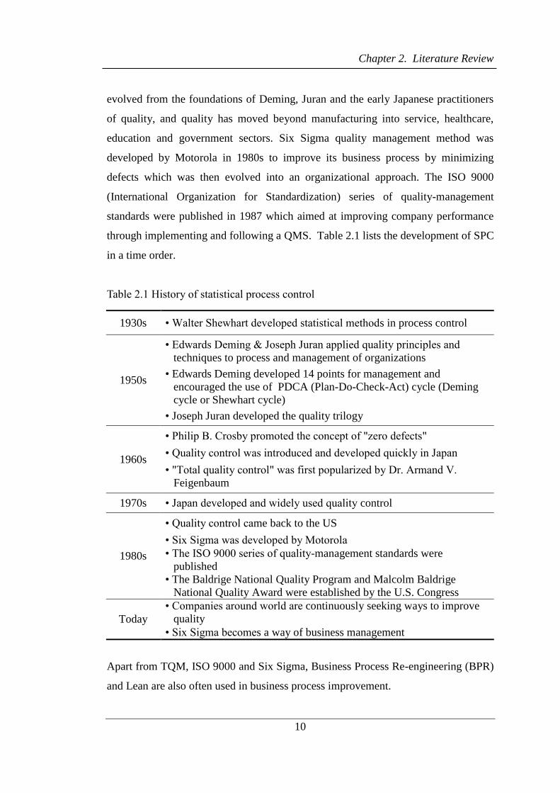
Chapter 2. Literature Review
10
evolved from the foundations of Deming, Juran and the early Japanese practitioners
of quality, and quality has moved beyond manufacturing into service, healthcare,
education and government sectors. Six Sigma quality management method was
developed by Motorola in 1980s to improve its business process by minimizing
defects which was then evolved into an organizational approach. The ISO 9000
(International Organization for Standardization) series of quality-management
standards were published in 1987 which aimed at improving company performance
through implementing and following a QMS. Table 2.1 lists the development of SPC
in a time order.
Table 2.1 History of statistical process control
1930s • Walter Shewhart developed statistical methods in process control
1950s
• Edwards Deming & Joseph Juran applied quality principles and
techniques to process and management of organizations
• Edwards Deming developed 14 points for management and
encouraged the use of PDCA (Plan-Do-Check-Act) cycle (Deming
cycle or Shewhart cycle)
• Joseph Juran developed the quality trilogy
1960s
• Philip B. Crosby promoted the concept of "zero defects"
• Quality control was introduced and developed quickly in Japan
• "Total quality control" was first popularized by Dr. Armand V.
Feigenbaum
1970s • Japan developed and widely used quality control
1980s
• Quality control came back to the US
• Six Sigma was developed by Motorola
• The ISO 9000 series of quality-management standards were
published
• The Baldrige National Quality Program and Malcolm Baldrige
National Quality Award were established by the U.S. Congress
Today
• Companies around world are continuously seeking ways to improve
quality
• Six Sigma becomes a way of business management
Apart from TQM, ISO 9000 and Six Sigma, Business Process Re-engineering (BPR)
and Lean are also often used in business process improvement.

Chapter 2. Literature Review
11
2.2.2 Total Quality Management (TQM)
TQM, an umbrella term for company-wide quality improvement efforts, came from
the work of Deming and his direction in the rebuilding of Japanese production
beginning in 1950 (Black and Revere, 2006). In 1969, the first international
conference on quality control was held in Tokyo where the term “total quality” was
used by Dr. Armand Vallin Feigenbaum in his paper for the first time, and referred to
wider issues compared with the traditional understanding of quality, such as
planning, organisation and management responsibility. Ishikawa presented a paper
explaining how “total quality control” in Japan was different, its meaning
“companywide quality control (CWQC)”, and describing how all employees, from
top management to the workers, must study and participate in quality control
(Charantimath, 2011). Towards the end of the 1970s, America was facing a major
quality crisis from the competition of Japan which started attracting attention from
national legislators, administrators and the media. A 1980 NBC-TV News special
report, “If Japan Can… Why Can’t We?” highlighted how Japan had captured the
world auto and electronics markets. Finally, U.S. organizations started their quality
improvement by replicating CWQC which was later known as TQM. It is grounded
in the original Deming cycle PDCA. Tobin (1990) defined TQM as a totally
integrated programme for gaining competitive advantages by continuously
improving every facet of organizational culture. TQM has soon become the
prevailing business strategy adopted by industries around the world. The TQM
approach advocates that (Kelada, 1996):
The concept of quality extends well beyond the quality of the product.
Everyone in an organization participates in the quality improvement process.
Top management, starting with the Chief Executive Officer (CEO) and chief
operations officer, demonstrates strong involvement and leadership.
The emphasis is laid on attaining and surpassing customer satisfaction.
External partners also participate in the total quality effort.

Chapter 2. Literature Review
12
Many studies compare TQM with Six Sigma (Andersson et al., 2006; Klefsjö et al.,
2001; Cheng, 2009; Black and Revere, 2006). Brun (2011) described TQM as the
father of Six Sigma as many of the principles constituting the basis of TQM are also
paramount in Six Sigma. It employs some of the same tools and techniques of TQM.
They both share similar philosophy - continuous quality improvement is essential to
long term business success and they both are top-down methods believing the
importance of top management support in successful quality management. Klefsjö et
al. (2001) stated that Six Sigma should be regarded as a methodology within the
larger framework of TQM in that Six Sigma supports all the six values in TQM.
Although it has been popular for many years, the passion for TQM has faded
whereas Six Sigma has been receiving increasing attention. According to Harari
(1993) study, only about one-fifth, or at best one-third, of the TQM programmes in
the US and Europe have achieved significant or even tangible improvements in
quality, productivity, competitiveness or financial results. Among the reasons cited
for TQM failure are excessive bureaucracy, focus on internal processes, avoidance of
genuine organizational reform, faddism, and lack of innovation within the corporate
culture (Green, 2007). Pande et al. (2000) outlined some reasons for the superiority
of Six Sigma compared to TQM (Table 2.2).
2.2.3 ISO 9001
The low probability of success has driven companies away from TQM. They opted
for ISO 9001 which is a management system standard. ISO 9001 is a set of standards
for process management by following which a company can be certified through
external auditing. ISO defines a standard as “a document that provides requirements,
specifications, guidelines or characteristics that can be used consistently to ensure
that materials, products, processes and services are fit for their purpose” (ISO, 2014).
It aims at improving company performance through implementing and following a
QMS. It is claimed by the ISO that their international standards can help businesses
achieve cost saving, enhance customer satisfaction, access new markets and increase

Chapter 2. Literature Review
13
market share, etc. (ISO, 2014).
Table 2.2 Six Sigma vs. TQM
TQM Six Sigma
Lack of integration, not connected with
strategy and performance High level of integration
Leadership apathy Leadership at the vanguard
A fuzzy concept A consistently repeated, simple message
An unclear goal Ambitious goal
Strong attitudes or technical fanaticism Adapting tools and degree of rigor to
the circumstances
Failure to break down internal barriers Priority on cross functional process
management
Incremental vs exponential change Incremental exponential change
Ineffective training Effective belt system
Focus on product quality Attention to all business processes
The ISO is a voluntary worldwide federation of national standards bodies from 165
countries (as of 2014) with each one representing one country, including the
American National Standards Institute (ANSI), and the British Standards Institute
(BSI). It was established in 1947 with the mission of promoting the development of
standardization and related activities in the world with a view to facilitating the
international exchange of goods and services, and to developing cooperation in the
spheres of intellectual, scientific, technological and economic activity (ANSI, 2014).
Its best-selling and most widely known document - ISO 9001, was published in 1987
together with ISO 9002 and ISO 9003. They have been revised several times by the
standing technical committees and advisory groups with the last time in 2008.
Among all the ISO 9000 family standards, ISO 9001:2008 is the only one that can be
certified to. The ISO 9000 family addresses various aspects of quality management.
Its standards provide guidance and tools for companies and organizations who want
to ensure that their products and services consistently meet customers’ requirements,

Chapter 2. Literature Review
14
and the quality is consistently improved (ISO, 2014). ISO 9001 series were
developed and revised based on eight quality management principles (ISO, 2012)
that can be used by management to help their organization towards improved
performance and higher quality output:
Customer focus.
Leadership.
Involvement of people.
Process approach.
System approach to management.
Continual improvement.
Factual approach to decision making.
Mutually beneficial supplier relationships.
Right from the days of the release of the ISO 9000 series standards, ISO 9001
certifications have been occurring with high momentum in the majority parts of the
world (Karthi et al., 2012). Since its first release in 1987, the total number of
organizations certified to ISO 9001 has exceeded one million and covers a wide
range of industries. Seddon (1997) stated that the main practical advantage of ISO
9000 is that it enables organisations to tender for business they might otherwise not
get. Douglas et al. (2003) study revealed that the top ranking benefits of ISO 9000
include organisational consistency, improved efficiency/performance, improved
customer service and management control. Corbett et al. (2005) found that ISO 9000
indeed increases productivity. Poksinska et al. (2002) believed that ISO 9000
standards can be applied uniformly to organisations of any size or description, which
is another important reason for its popularity.
However, ISO 9000 has received many criticisms. In Douglas et al. (2003) research,
49 percent of the survey respondents considered their organisations did not achieve
any benefit with regard to reduced costs or waste and 53 percent perceived no
benefits with respect to staff motivation/retention. Furthermore, Tennant (2001)

Chapter 2. Literature Review
15
pointed out that once a certificate has been achieved, quality standardization perhaps
has little to motivate further improvement.
ISO9001 and Six Sigma are complementary to each other. There are studies
suggesting the integration of Six Sigma and ISO9001 certification where ISO 9001
can be used to identify existing problems and Six Sigma can be used to resolve them
(Pfeifer et al., 2004; Karthi et al., 2012; Lupan et al., 2005).
2.2.4 Business Process Reengineering (BPR)
BPR was first bought to the attention of the business world by Hammer and Champy
(1993), who defined BPR as “The fundamental rethinking and radical design of
business processes to achieve dramatic improvement in critical, contemporary
measures of performance such as cost, quality, service and speed”. It aims at
improving business performance by identifying opportunities for new business, for
outsourcing, for improving business efficiency and for areas within the business
where technology can be used to support business processes (Lindsay et al., 2003). It
restructures the operation by challenging each step involved and redesigns the whole
working process. BPR assumes that the current processes in a business are
inapplicable and suggests completely new processes to be implemented. Although it
was not the intention, BPR becomes associated with company downsizing and
redundancy. Goel and Chen (2008) suggested that re-engineering often results in
huge short-term costs that need to be amortized over several years through increased
future revenues resulting from the reengineering. Six Sigma, however, is a quality
improvement programme with a clear methodology to improve current processes by
reducing variation. Some differences between BPR and Six Sigma are listed in Table
2.3.
With the implementation of Six Sigma, some companies, such as Motorola and GE,
realized that merely removing variation from processes and products could not meet
the customer’s requirement who demanded improved products. Design for Six Sigma

Chapter 2. Literature Review
16
(DFSS) was therefore developed. It is not as mature as DMAIC and there is no
standard defined methodology for DFSS. BPR and DFSS are all for process redesign
but different in some ways given the fact that DFSS is based on Six Sigma’s
statistical thinking and customer focus. In Six Sigma, redesign is only a step to take
if improvements are at their peak but there is still a large gap between customer
requirements and process performance. Six sigma is often adopted as a management
methodology that utilizes measures as a foundational tool for BPR. Pande et al.
(2000) stated that two conditions must be met in order for the process redesign to
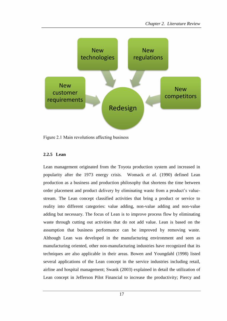
work. They are “a major need, threat or opportunity exists” and “ready and willing to
take on the risk”. The main revolutions affecting business are “new technologies”,
“new regulations”, “new competitors” and “new customer requirements” (Figure
2.1). When these emerge, a redesign of the process may need to be considered.
Table 2.3 BPR vs. Six Sigma
BPR Six Sigma
Focus on cost, time, efficiency and productivity
but not customers
Emphasis on customer
requirements
Large scale, long execution times Project can be small scale and
completed in short time
Normally the execution needs the involvement of
consulting firms
Can be executed by internal
resources through effective training
Fundamental change of process, radical change Incremental and continuous
improvement on the current process
Often lead to redundancy Lead to improved performance
May need long time to see the benefit achieved Improvement can be visible at
projects completion
IT is an enabler Using statistical tools and controls
Lead to structure change Lead to culture change
Does not have a standard methodology
Use DMAIC (Define-Measure-
Analyse-Improve-Control) as the
methodology
Chapter 2. Literature Review
17
Figure 2.1 Main revolutions affecting business
2.2.5 Lean
Lean management originated from the Toyota production system and increased in
popularity after the 1973 energy crisis. Womack et al. (1990) defined Lean
production as a business and production philosophy that shortens the time between
order placement and product delivery by eliminating waste from a product’s value-
stream. The Lean concept classified activities that bring a product or service to
reality into different categories: value adding, non-value adding and non-value
adding but necessary. The focus of Lean is to improve process flow by eliminating
waste through cutting out activities that do not add value. Lean is based on the
assumption that business performance can be improved by removing waste.
Although Lean was developed in the manufacturing environment and seen as
manufacturing oriented, other non-manufacturing industries have recognized that its
techniques are also applicable in their areas. Bowen and Youngdahl (1998) listed
several applications of the Lean concept in the service industries including retail,
airline and hospital management; Swank (2003) explained in detail the utilization of
Lean concept in Jefferson Pilot Financial to increase the productivity; Piercy and
Redesign
New customer
requirements
New technologies
New regulations
New competitors

Chapter 2. Literature Review
18
Rich (2009) examined the applicability of Lean concept in a call centre to meet
customers’ requirement for “one-stop” call handling by redesigning the call handling
process. Most researchers agreed that there is more commonality between Lean and
Six Sigma tools and practices than differences (Shah et al., 2008). Lean and Six
Sigma are often considered to offer features which complement each other and are
increasingly being integrated in practice, but there is no consensus method
(Proudlove et al., 2008). However, the DMAIC, as a logical, proven and solid
approach, is applicable even in Lean-Six Sigma.
There are still many fundamental differences between the two methods. The relevant
literature suggested that the Lean concept is best used for reducing wastes, improving
efficiency of a process, reducing process time and improving space utilization, etc.,
while, Six Sigma is best used to reduce variation and identify root causes so as to
improve performance. The differences between the two methods mainly lay in their
objectives. Table 2.4 provides a comparison between the two methods.
Throughout the history of quality control, many approaches have set standards in
quality. Apart from the ones reviewed above, some other well recognized quality
control methods are listed in Table 2.5. However, due to their less relationship with
Six Sigma, they have only been briefly introduced in this work.
2.3 Review of Six Sigma
2.3.1 History of Six Sigma
Six Sigma can be rooted back to the efforts of Joseph Juran and W. Edwards
Deming. Their programmes for TQM in Japan, led to the adoption of the Six Sigma
philosophy by Motorola in the 1980s, when Motorola found itself unable to compete
in the consumer products market with Japanese companies. Its senior executive Art
Sundry's famous critique, "Our quality stinks" accelerated the change process in
Motorola.

Chapter 2. Literature Review
19
Table 2.4 Lean vs. Six Sigma
Lean Six Sigma
Theory / objective
Improve business performance / flow
time by removing waste and
streamlining process flow
Improve process
performance by
reducing variation
Application
methodology
Identify value desired by customers
Identify value stream
Make flow continuously
Introduce Pull
Manage towards perfection
(less strong than DMAIC)
DMAIC
Use of Data Less common Data intensive
Focus Process flow Variation, process
defects
Assumption Business performance can be improved
by removing waste
Problem exists but
the causes are
unknown.
Targeting problem Flow problem, more visible problems
Good for root-cause,
solution unknown
problems
Approach Operational, bottom-up approach Top down approach
Training Training while working along Designed structural
training
Table 2.5 Some quality control methods with a brief description
Taguchi Method A statistical method developed by Genichi Taguchi to improve quality.
The main objective in the Taguchi method is to design robust systems that
are reliable under uncontrollable conditions.
Kaizen
A Japanese word for improvement, carrying the connotation in industry of
all the non-contracted and partially contracted activities. Kaizen is defined
by Brunet and New (2003) as a method consisting of pervasive and
continual activities, outside the contributor's explicit contractual roles, to
identify and achieve outcomes that he believes contribute to the
organisational goals.
Quality Function
Deployment
(QFD)
An overall concept that provides a means of translating customer
requirements into the appropriate technical requirements for each stage of
product development and production (i.e., marketing strategies, planning,
product design and engineering, prototype evaluation, production process
development, production, sales) (Sullivan, 1986).
Zero Defect
Programme
Developed by Mr. Philip Crosby and has emerged as a trending concept in
quality management to eliminate defects. Zero defects defines a way of
thinking and doing. It emphasises that defects are not acceptable and
everyone should do things right the first time.

Chapter 2. Literature Review
20
Like the American business style in the early 80s, Motorola was keeping its customer
happy by reacting to (correcting) problems in the field, such as, large in-house repair
facilities to fix anything it could find before it got into the field and many repair
shops in the field to ensure that the customer receives quick service. As a result, the
prevailing view was that quality costs extra money. But Sundry saw that quality
through reaction is expensive. It takes a lot to support a reaction strategy: more
people, more material, more steps, more time and especially more money (Persse,
2006). Bill Smith subsequently formulated the particulars of the Six Sigma
methodology at Motorola in 1986. At the time, Six Sigma offered Motorola a simple
and consistent way to track and compare performance to customer requirements and
an ambitious target of practically-perfect quality (Pande et al., 2000) . In 1988
Motorola became the first company to capture the prestigious Malcolm Baldrige
award. The following year, Motorola was awarded the Nikkei Award for
manufacturing from Japan for creative excellence in products and service. Motorola
had spent USD170 million on workers’ education and training from 1983 to 1987,
among which 40 percent in 1987 was devoted to quality matters. Until 1997, a
decade from the beginning of the Six Sigma programme, Motorola had gone from a
company in jeopardy to a market leader with its sales increasing by 20% each year
and cumulative savings of USD14 billion (Pande et al., 2000).
Since the success of Six Sigma in Motorola, and particularly from 1995, an
exponentially growing number of global firms have launched Six Sigma. Six Sigma
became well known after Jack Welch made it a central focus of his business strategy
in GE in 1995. He set the goal of becoming a Six Sigma quality company by 2000, 5
years less than Motorola. While Motorola has used Six Sigma to stay in business, for
GE it was used to strengthen an already thriving company. Six Sigma was the
most ambitious undertaking GE had ever taken. They believed that Six Sigma can
change GE from one of the great companies to the greatest company in the world
business. GE’s focus on quality started in the late 1980s with the launch of the
“Work-Out” programme that opened GE culture to ideas from everyone and
everywhere. The resultant learning environment prepared the ground for Six Sigma.

Chapter 2. Literature Review
21
GE has made Six Sigma a far broader concept than improving quality by reducing
defects; it became a leadership development programme that can make a
transformation of a company.
Six Sigma has been widely reckoned as one of the most useful process improvement
and quality management programmes available. Other early adopters of Six Sigma
who achieved well-publicized success include Honeywell (previously known as
AlliedSignal), Citibank, Sony and GE (Antony and Banuelas, 2001).
The beauty of Six Sigma is that it can be used not only as an operational strategy to
reduce the number of defects but also as a business strategy to improve business
processes and evolve new business models (Kumar et al., 2008). Therefore, although
initially applied in manufacturing industries, Six Sigma has now been widely
appreciated across other sectors.
2.3.2 Definition of Six Sigma
There are different perspectives on what “Six Sigma” is. Business media often
describes Six Sigma as a “highly technical method used by engineers and
statisticians to fine-tune products and processes” (Pande et al., 2000). For many
business organisations, it simply means “a measure of quality that strives for near
perfection”. They are all true, in part. Taking references from Motorola, Six Sigma
can be defined and understood at three distinct levels: metric, methodology and
management system.
As a metric: The foundation of Six Sigma lies in statistical thinking. Sigma,
transliteration of Greek letter σ, means standard deviation in statistics and reflects the
degree of deviation. Six-Sigma means six-time standard deviation between the
average and the lower or upper limit. A sigma quality level indicates the frequency
that defects are likely to occur. Higher sigma quality level is a sign that processes
would produce fewer defects. One sigma level represents 691462.5 defects per

Chapter 2. Literature Review
22
million opportunities (DPMO), which translates to a percentage of non-defective
outputs of 30.854%. The “Six Sigma” quality level is equal to 3.4 DPMO which
translates to 99.99966% non-defective outputs. Table 2.6 provides a simple list of the
Sigma levels with their associated DPMO values.
Table 2.6 Simplified sigma levels
Sigma level Non-defective output (%) DPMO
1 30.9 690,000
2 69.2 308,000
3 93.3 66,800
4 99.4 6,210
5 99.98 320
6 99.9997 3.4
As a methodology: Six Sigma is a systematic, highly disciplined, customer–centric
and profit–driven business improvement initiative that is based on rigorous process-
focused and project-driven methodology. Six Sigma uses data and statistical analysis
to measure and improve company’s operational performance via the DMAIC
framework (Tang et al., 2007).
As a management system: It is often discovered that one of the difficulties facing Six
Sigma projects is sustainability. Simply applying the methodology is not sufficient to
drive the desired breakthrough improvements and results that are sustainable over
time. It is found that sustainable and breakthrough improvements are realized by
those organizations whose leadership has embraced Six Sigma and incorporated it
into their vision, strategies and business objectives. When practiced as a management
system, Six Sigma is a high performance system for executing business strategy.
Six Sigma has evolved over the last two decades and so has its definition. There
exists no unique definition of Six Sigma. However, in business terms, Six Sigma can
Chapter 2. Literature Review
23
be defined as: A business improvement strategy of applying a statistical
methodology, to identify and eliminate causes of defects & variations, and to achieve
improvement of business profitability, reduction of cost of poor quality (COPQ) and
improvement of the effectiveness and efficiency of all operations so as to meet or
even exceed customers’ needs and expectations.
The tools used in Six Sigma are by no means new, but it is not merely repackaging
the old concepts to create a new term for project management. It integrates many
existing techniques which are appropriate in its implementation and organizes them
into a programme that can be built into business strategy and culture in order to
achieve breakthrough and sustainable process improvement. Six Sigma includes as
much effort on people excellence as technical excellence.
2.3.3 Benefits of Six Sigma
Six Sigma has enjoyed an unprecedented long period of popularity. It attracts
organizations by achieving great benefits including tangible results, such as cost
saving and waste reduction. Table 2.7 shows the benefits obtained from Six-Sigma
applications in some large manufacturing companies (Mehrjerdi, 2011; Kwak and
Anbari, 2006).
One of Six Sigma’s most important elements is customer focus. It is suggested in
Aboelmaged (2010)’s research that the most cited benefit of Six Sigma in the
literature is “customer satisfaction”. The study also summarized the benefits that Six
Sigma can achieve for both manufacturing and service organisations through the
literature review of previous relevant research. Antony (2004a) has also revealed
some of the benefits of applying Six Sigma in the service industries (Table 2.8).

Chapter 2. Literature Review
24
Table 2.7 Reported benefits and savings through Six Sigma in the manufacturing
sector
Company name Metric/Measures Benefits/savings
Motorola (1992) In-process defect levels 150 times reduction
Allied Signal / Honeywell (1999) Financial $600 million annual savings
since 1994
Raytheon/aircraft integration systems Depot maintenance inspection
time
Reduced 88% as measured in
days
Hughes aircraft’s missiles systems group
/ wave soldering
Quality/productivity Improved 1,000%/ improved
500%
GE (1999) Financial $2 billion
Motorola (1999) (www.motorala.com) Financial $15 billion in 11 years
Dow Chemical/Rail Delivery Project
(The Dow Chemical Company )
Financial $2.45 million in capital
expenditures
Du Pont/Yerkes Plant in New York
(2000)
Financial More than $25 million savings
Telefonica de espana (2001) Financial €30 millions in the first ten
months
Texas Instruments Financial $600 millions
Johnson and Johnson Financial $500 millions
Honeywell Financial $1.2 billions
Table 2.8 Benefits of Six Sigma in both manufacturing and service organisations
Manufacturing • reduction in process variability
• reduction in in-process defect levels
• reduction in maintenance inspection time
• improving capacity cycle time
• improving inventory on-time delivery
• increasing savings in capital expenditures
• increase in profitability
• reduction of operational costs
• reduction in the COPQ
• increase in productivity
• reduction of cycle time

Chapter 2. Literature Review
25
• reduction of customer complaints
• improved sales and reduced inspection
Service organizations • improved accuracy of resources allocation
• improving accuracy of reporting
• reduced documentary defects
• improving timely and accurate claims reimbursement
• streamlining the process of service delivery
• reduced inventory of equipment
• reduced service preparation times
• improved customer satisfaction
• reduced defect rate in service processes
• reduced variability of key service processes
• transformation of organizational culture from fire-fighting
mode to fire-prevention mode with the attitude of continuous
improvement of service process performance
• reduced process cycle time and hence achieve faster service
delivery
• reduced service operational costs
• increased market share
• improved cross-functional teamwork across the entire
organization
• increased employee morale
• reduced number of non-value added steps in critical business
processes through systematic elimination
• leading to faster delivery of service, reduced COPQ (costs
associated with late delivery, customer complaints, costs
associated with misdirected problem solving, etc.)
• increased awareness of various problem solving tools and
techniques
• leading to greater job satisfaction for employees
• improved consistency level of service through systematic
reduction of process variability and effective management
decisions due to reliance on data and facts rather than
assumptions and gut-feelings
• improved effective management decisions due to reliance on
data and facts rather than assumptions and gut-feelings.

Chapter 2. Literature Review
26
Apart from those listed in Table 2.8, what also makes Six Sigma so attractive is the
fact that the improvements are continuous and sustainable by changing the company
culture and creating a learning organization. Pande et al. (2000) stated that Six Sigma
can generate sustained success, set a performance goal for everyone, enhance value
to customers, accelerate the rate of improvement, promote learning and “cross-
pollination” and execute strategic change.
2.3.4 Methodology
Six Sigma is a project-based structured methodology aiming at reducing process
defects and variability by taking account of customer requirements. Its
implementation uses a five-step DMAIC methodology (Figure 2.2). DMAIC
provides a roadmap with tools for conducting projects. Although similar to the
PDCA cycle, the DMAIC emphasises results measurement and control, and has
extensive use of statistics. DMAIC model has been adopted by many companies in
Six Sigma implementation, such as ABB, Caterpillar and Intersil. It provides a
consistent approach for organizations in adopting Six Sigma. DMAIC focuses on
“customer needs” and “continuous measurement” to achieve improvement on current
processes which are essential aspects in shipping company quality improvement. In
the meantime, it also offers the opportunity to redesign the processes if it becomes
necessary. Six Sigma did not introduce new tools, instead, it provides a different
methodology for implementation which focuses on business infrastructure and
bottom-line results.
2.3.5 Critical Success Factors (CSFs)
The successful implementation of Six Sigma projects is much more than just
understanding the DMAIC tool set. Zimmerman and Weiss (2005) quoted a survey
conducted by Aviation Week magazine in which among major aerospace companies,
less than 50% expressed satisfaction on the results from Six Sigma projects, around
20% were somewhat satisfied and nearly 30% were dissatisfied. CSFs are those
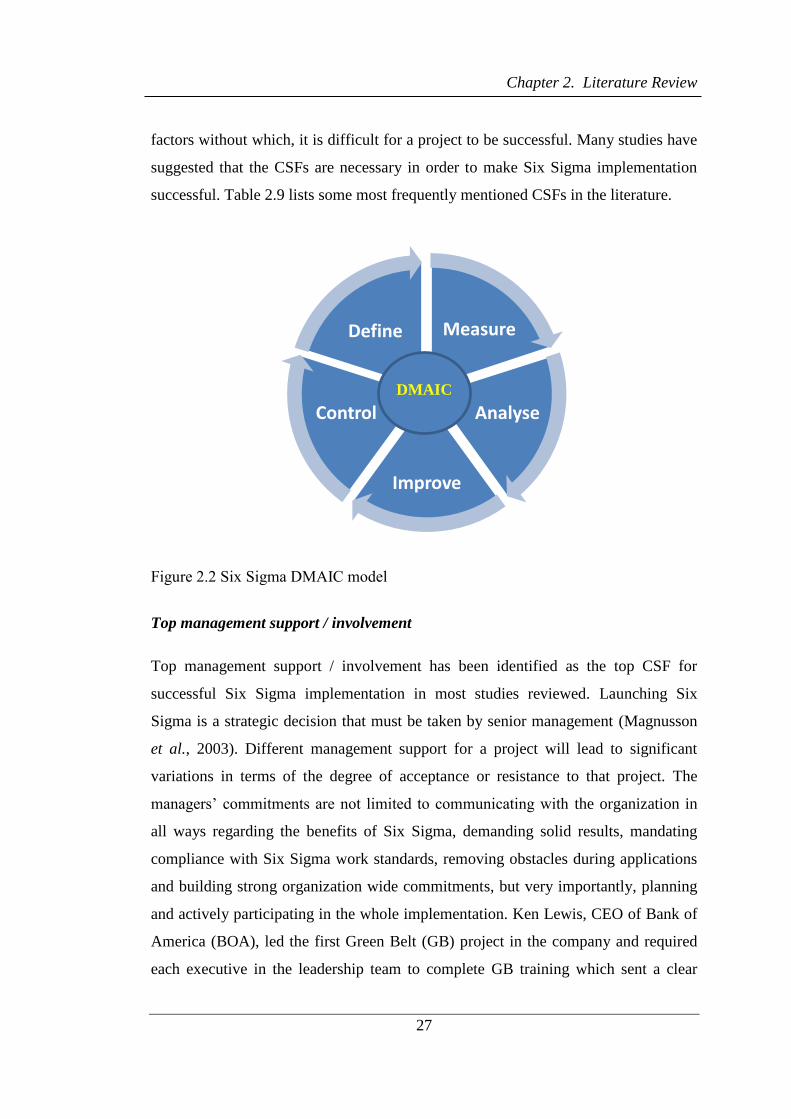
Chapter 2. Literature Review
27
factors without which, it is difficult for a project to be successful. Many studies have
suggested that the CSFs are necessary in order to make Six Sigma implementation
successful. Table 2.9 lists some most frequently mentioned CSFs in the literature.
Figure 2.2 Six Sigma DMAIC model
Top management support / involvement
Top management support / involvement has been identified as the top CSF for
successful Six Sigma implementation in most studies reviewed. Launching Six
Sigma is a strategic decision that must be taken by senior management (Magnusson
et al., 2003). Different management support for a project will lead to significant
variations in terms of the degree of acceptance or resistance to that project. The
managers’ commitments are not limited to communicating with the organization in
all ways regarding the benefits of Six Sigma, demanding solid results, mandating
compliance with Six Sigma work standards, removing obstacles during applications
and building strong organization wide commitments, but very importantly, planning
and actively participating in the whole implementation. Ken Lewis, CEO of Bank of
America (BOA), led the first Green Belt (GB) project in the company and required
each executive in the leadership team to complete GB training which sent a clear
Measure
Analyse
Improve
Control
Define
DMAIC

Chapter 2. Literature Review
28
message of the support from the most senior leadership. Robert W. Galvin, the
former CEO and chairman of Motorola, always asked for the Six Sigma reports from
different divisions first in operation meetings; Dan Burnham, CEO of Raytheon
personally teaches Six Sigma principles to other leaders in his company; Mike
Parker, CEO of Dow Chemical participates actively and visibly in all the “waves” of
the company’s Black Belt (BB) training at its Six Sigma training centre in Atlanta,
Georgia (Byrne, 2003). The success of Six Sigma lies in the commitment of top
management and can only be initialized once the top manager’s commitments are
established.
Table 2.9 CSFs for successful implementation of Six Sigma
Hen
der
son
and
Ev
ans
(200
0)
Pan
de
et a
l. (
20
00)
Co
ron
ado
an
d A
nto
ny
(2
00
2)
By
rne
(200
3)
An
ton
y (
20
04
a)
Bre
wer
an
d B
agra
noff
(2
004
)
No
nth
alee
rak
an
d H
end
ry (
200
8)
Fir
ka
(20
10
)
Top management support/
involvement √ √ √ √ √ √ √ √
Training √ √ √ √ √ √ √
Statistical tools √ √ √
√ √
√
Project selection
√
√ √
√
Organisation infrastructure √
√
√
√
Connect to business strategy
√ √
√
√
Culture change
√
√ √
√
Customer focus
√ √
√
√
Rewards and recognition
√ √
√ √

Chapter 2. Literature Review
29
Training
One of the unique characteristics of Six Sigma compared with other quality
methodologies is to have trained personnel leading and participating in projects.
Training is a key ingredient to achieve success by following the Six Sigma way
(Pande et al., 2000). Continuous learning contributes to sustaining the results
achieved from Six Sigma and continuously renewing and improving them. Six Sigma
training should not be limited to belts (Table 3.1 provides a detailed explanation of
the belt system in Six Sigma), although their training is more in-depth and
comprehensive, it should be cascaded throughout the organisation. Operators are the
people who carry out the daily tasks and the main contributors to the quality of
products and services. GE’s Six Sigma implementation started with a heavy
emphasis on training, 4% - 5% people were taken out of their daily task and trained
full time to the most advanced level; another 50% were trained to intermediate level
and “green belt training” was delivered to all its employees. It is worth mentioning
that GE’s experience in implementation of Six Sigma shows that the best of training
and mentoring efforts would crumble without effective leadership (Nayab, 2011).
Effective training of BBs and any other Six Sigma project leaders is not limited to
the knowledge and tools in Six Sigma, such as statistical methods, analytical
techniques and measurement tools, but also project management and people skills,
such as leading change and team collaboration. The contents of Six Sigma training
could vary from different needs and providers (external and internal). Generally, the
course for BBs is comprehensive and aiming at those who will become full-time Six
Sigma project leaders/experts; the course for GBs covers a range of broad enough
contents to prepare them for contributing to or managing projects, the course for
operators needs to include basic concepts and knowledge of Six Sigma and some
statistical tools that can be useful in their daily tasks.
Training indeed costs. Is it worth it? Most successful companies believe that training
is worth the investment. Motorola invested USD50 million annually in Six Sigma
training from 1987 to 1992 which represents 40 percent of their total training budget.

Chapter 2. Literature Review
30
The reported return on investment ratio was 29:1, as Motorola estimated savings of
USD2.4 billion from Six Sigma improvement projects during the same period
(Magnusson et al., 2003).
Statistical tools
Six Sigma does not create any new statistical method, but adopts existing tools to
improve processes and products through the DMAIC framework. Therefore, the
ability of selecting and using the right tools according to different projects and issues
is essential to the success of a project. Some frequently used tools are discussed in
the next section.
Project selection
Six Sigma is a project-driven methodology. Selecting appropriate projects is essential
to ensure the success of Six Sigma application. Breyfogle (2001) suggested that
project selection is one of the most important factors for achieving success in Six
Sigma applications. Zimmerman and Weiss (2005) believed that failure of correctly
identifying and prioritizing improvement projects is one of the reasons many Six
Sigma programmes fail. Pande et al. (2000) stated that good project selection is itself
a process and if properly carried out, the potential benefits of Six Sigma can be
substantially improved. Identification of high-impact projects at the initial stage of a
programme will result in significant breakthroughs in a rapid timeframe. A project
that is too large will cost valuable time as belts will struggle to cope. Selecting a Six
Sigma project has therefore been one of the most often discussed issues in today’s
Six Sigma research. It will be further discussed in Chapter 4 of this thesis.
Organisation infrastructure
Six Sigma represents a new way of working and it relies on the collection and
analysis of data and the use of numerous statistical tools for correcting defects
(Byrne, 2003). The implementation of Six Sigma is to be supported by a robust
Chapter 2. Literature Review
31
infrastructure. Organisation infrastructure includes both human resources and IT. A
company needs to have and be willing to provide adequate resources and investments
for the implementation as Six Sigma implementation will change the job of a small
but critical group of personnel who will become the catalyst of changes. It is
essential to ensure that the resources are available when needed and that clear
responsibilities are assigned according to the Six Sigma belt system. On the other
hand, measurement and analysis are key elements in Six Sigma which all require
extensive data from reliable systems. James Stanley, senior vice president of US
operations for Howmet International Corp., a GE Aircraft Engines supplier, suggests
“systems are vitally important. The systems have to give you data instantaneously . .
. the IT infrastructure could make or break the Six Sigma effort. Data gathering is
key” (Henderson and Evans, 2000). During the implementation, a company often
identifies the need for a modified or completely new measurement system. A well-
developed system can be used for not only collecting reliable and sufficient data but
also monitoring performance towards achieving sustainable results.
Connect to business strategy
Berger et al. (2007) suggested that deploying Six Sigma as a business strategy
through projects instead of tools is a more effective way to benefit from the time and
money invested in Six Sigma training. A good business strategy is one that can be
translated into quantifiable objectives. Six Sigma projects should be generated based
on the needs of achieving those objectives, and target on process and performance
bearing direct impacts on finance or operations linking to the strategy. The
contribution of a project should be clearly stated in terms of finance. The application
of Six Sigma requires a top-down management approach. Financial savings and
aligning with business strategy help to motivate the top management team so as to
achieve continuous improvement. Often the establishment of the connection between
Six Sigma and business strategy can become a breakthrough point for some
executives who might have resisted Six Sigma.

Chapter 2. Literature Review
32
Culture change
Six Sigma is “change”, changing the way of working, thinking, measuring,
monitoring and managing. It is about creating a culture of continuous improvement
and statistical thinking. Culture change is a prime factor to a lasting Six Sigma
programme. When change happens, people affected are often unsure and sometimes
afraid. “What have we done wrong?”, “what is going to happen to me” and “it has
always been the way of doing it” are some typical phrases mentioned. Companies
which succeeded in managing change have identified that the best way to tackle
resistance to change is through increased and sustained communication, motivation
and education (Coronado and Antony, 2002). It is important that all employees
understand the reason for the application of Six Sigma – identifying defects and
making improvement, instead of being penalized. It will also make a great difference
if employees are feeling responsible for the success of the Six Sigma programme and
seeing the benefits resulting from their efforts. Culture change is a gradual process
which once achieved, can make continuous improvement a gene of the business.
Customer focus
The philosophy of Six Sigma is to meet or exceed customers’ expectation. Meeting
customer requirements is the ultimate goal of Six Sigma. Correctly identified
customer needs and gaps for improvement set the target for a Six Sigma project. In
the meantime, considering and involving customers in Six Sigma implementation can
develop a trust relationship, create knowledge transfer and increase customer loyalty.
Rewards and recognition
Recognition and rewards play a valuable role in motivating team members and
sustaining the momentum of Six Sigma so as to establish a long term continuous
improvement culture in an organization. Samsung believes that meaningful
recognition and rewards for employees is one of the four factors that made Six Sigma

Chapter 2. Literature Review
33
successful throughout their international operations and culture (Yun and Chua,
2002). Shani and Docherty (2003) suggested that an effective reward system is
essential to the sustainable results of a change programme. On successful completion
of a project, leadership needs to identify ways to reward extraordinary participation
by employees which will also send positive messages to the organisation of Six
Sigma implementation. It helps to drive the enthusiasm throughout the organisation
from a top-down level and therefore better promotes a companywide
implementation.
2.4 Tools in Six Sigma
The systematic and rigorous tools associated with the Six Sigma of today were
mostly included when the method was first developed by Motorola. Although most
of the tools are not unique, they have been brought together to provide a well-stocked
toolbox. Goh (2011) states that the statistical tools used in Six Sigma are logically
aligned and integrated which is in response to the perception of “there is nothing new
in Six Sigma but a repackaging of old concepts”. Not all the tools are required to be
used in every project. Different tools are adopted in the individual phases of a
DMAIC cycle depending on the objectives. A brief review is given in this section of
some of frequently mentioned and applied tools in Six Sigma projects in the service
industries.
2.4.1 Project Charter
The Project Management Body of Knowledge (PMBOK) defines a project charter as
a document that formally authorizes a project (Gilchrist, 2012). A project charter
includes the information of business needs for the project, its scope, objectives and
participants. It is normally issued and/or approved by a project sponsor. A signed off
project charter is an agreement between the management and Six Sigma teams
regarding the expected project outcomes. It is the first step in the DMAIC cycle and

Chapter 2. Literature Review
34
takes place in the Define phase of a Six Sigma project. The purpose of a project
charter is to document the reasons for undertaking the project, its objectives and
constraints, scope and anticipated benefits, set the project direction and define the
measures of success, identify the main stakeholders and empower the project
manager with the authority to carry out the project. Project charter works as an
essential document which helps the project manager to effectively communicate with
project participants and stakeholders regarding the project information, sets clear
understanding of the responsibilities and accountabilities and provides motivation for
the project team.
A Six Sigma project charter contains several parts:
General information
Project title.
Project manager (BB or GB), sponsor, and mentor (Master Black Belt
(MBB).
Project start date.
Anticipated project end date.
Project overview
Business case / problem statement – outlines the business problems
that need to be addressed.
Project goals / objectives – describes the expected outcomes of the
project.
Expected financial benefits – provides all financial benefits.
Project scope – defines the boundaries of the project.
Major milestones – gives a breakdown of the anticipated project
progress.
Project teams – summarises the selected team members, their roles
and responsibilities.
Signatures

Chapter 2. Literature Review
35
Project charter signatures – obtain signature from project sponsor /
champion as an approval of the project.
Project closure signatures – Signed by project sponsor / champion
after the control phase as an agreement to accept the new process and
the official closure of the project.
A Project Charter is the major deliverable of the project initiation. The length of the
project charter is proportional to the size and complexity of the project.
2.4.2 Critical to Quality (CTQ) Tree
CTQ factors derive from voice of customer (VOC) and is a selection of the
characteristics that are critical to customers (mainly external customers), processes
(mainly internal customers and processes) and compliances (e.g. government and
industry regulator) (Magnusson et al., 2003). They may include the upper and lower
specification limits or any other factors related to the product or service (Yun and
Chun, 2008). CTQs usually must be interpreted from the qualitative statements of
the customers to a manageable quantitative business specification (He et al., 2010).
CTQ tree is a diagram to decompose broad customer requirements into specific,
actionable business statements or measures that can be measured for meeting
customer expectations. It is often seen in the define phase of a Six Sigma Project.
Identifying customer needs and creating a CTQ tree are time consuming processes
and can involve several steps:
Identify customers for the process to be improved.
Collect customer requirements (VOC) – VOC can be obtained through
customer surveys, interviews or expert judgements (brainstorming).
Identify quality drivers for the requirements – These are also collected from
customers or experts.
Identify measurable performance requirements for each quality driver –
Validation from customers is desirable regarding the identified requirements.

Chapter 2. Literature Review
36
An example CTQ tree is presented in Figure 2.3 , where “I want good customer
service” is a broad statement from customers and the quality drivers to the good
customer service are “minimum mistakes” and “speedy response” which are finally
presented by the measureable requirements “accuracy rate of invoices”, “percentage
of queries due to internal error”, “time taken to return phone calls” and “time taken
to resolve queries”.
Figure 2.3 Example of a CTQ tree
During a project, several CTQ trees may be needed depending on the requirements of
customers. Although most often used as a part of Six Sigma, CTQ tree can make an
effective tool in various situations where quantifiable measures need to be identified
from general and qualitative requirements.
2.4.3 Process Mapping
A process is a series of activities which takes inputs, transforms them by adding
value, and produces outputs for customers (Figure 2.4). It is extremely difficult to
improve a process without a thorough understanding of its steps and this may lead to
VOC: I want good customer service
Minimum mistakes
Accuracy rate of invoices
% of queries due to internal errors
Speedy responses
Time taken to return phone calls
Time takes to resolve queries
Customer needs Drivers Requirements (CTQs)

Chapter 2. Literature Review
37
costly mistakes. Process mapping is a tool to create process maps by gathering,
organizing and presenting details of a process. A process map is a workflow diagram
presenting the sequences of actions that comprise a process. It visualizes activities
and interacts in a process to enable an organization to have an clear understanding of
their current performance and provides opportunities to quickly identify bottlenecks,
process imbalances and many other issues, by resolving which, the process can be
improved. Many quality improvements in the service industries rely on a complete
and accurate process map. The objective of the process mapping is to document and
understand a process and improve it. Process mapping can be used in the define,
measure and analyse phases in a Six Sigma project.
Figure 2.4 A process model
Process mapping is one of the easiest to grasp tools yet extremely effective. It can be
carried out with certain guidance.
Define the process to be measured and boundaries (start and end points).
List first step and outline the major steps on the process.
Identify detailed steps and their sequences.
Draw symbols for each step.
Add supplementary information.
Inputs
Xs
Outputs
Ys
Operation process
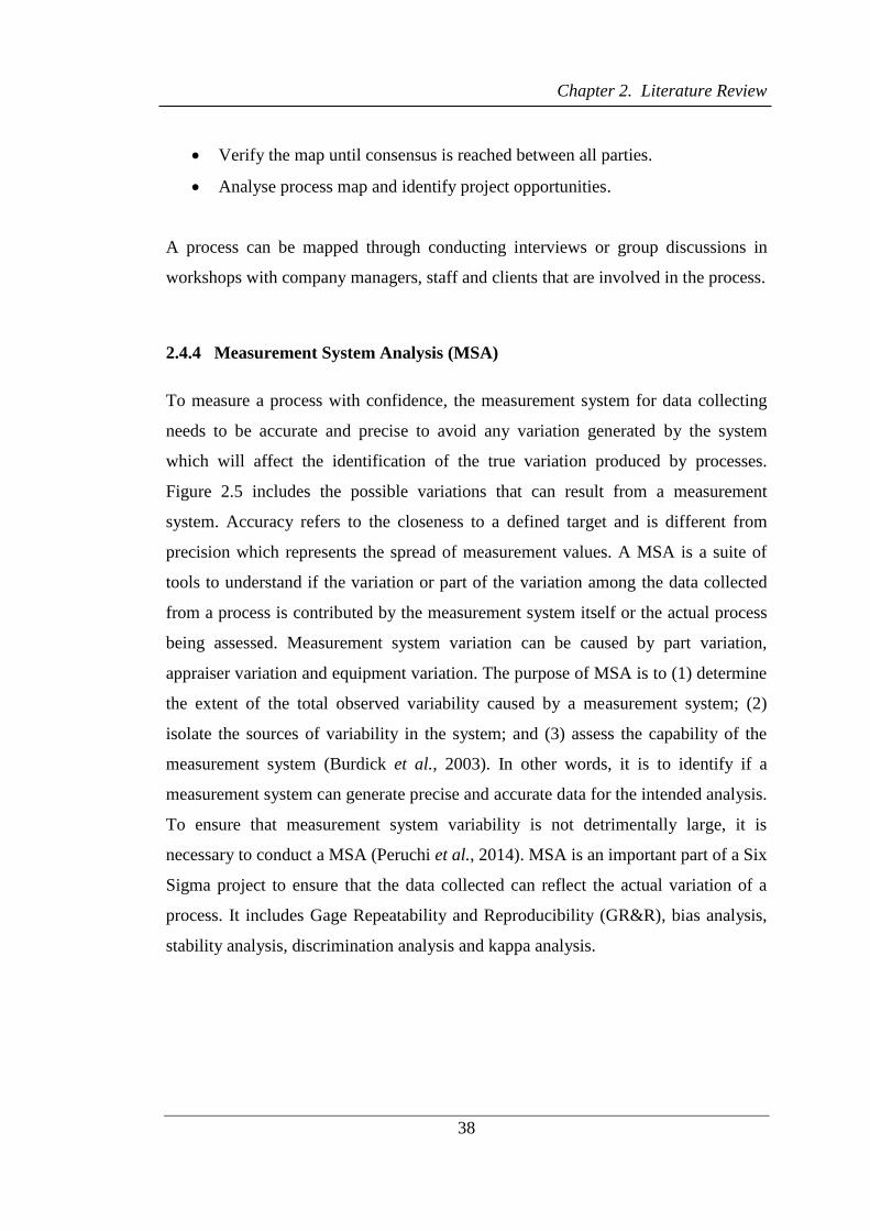
Chapter 2. Literature Review
38
Verify the map until consensus is reached between all parties.
Analyse process map and identify project opportunities.
A process can be mapped through conducting interviews or group discussions in
workshops with company managers, staff and clients that are involved in the process.
2.4.4 Measurement System Analysis (MSA)
To measure a process with confidence, the measurement system for data collecting
needs to be accurate and precise to avoid any variation generated by the system
which will affect the identification of the true variation produced by processes.
Figure 2.5 includes the possible variations that can result from a measurement
system. Accuracy refers to the closeness to a defined target and is different from
precision which represents the spread of measurement values. A MSA is a suite of
tools to understand if the variation or part of the variation among the data collected
from a process is contributed by the measurement system itself or the actual process
being assessed. Measurement system variation can be caused by part variation,
appraiser variation and equipment variation. The purpose of MSA is to (1) determine
the extent of the total observed variability caused by a measurement system; (2)
isolate the sources of variability in the system; and (3) assess the capability of the
measurement system (Burdick et al., 2003). In other words, it is to identify if a
measurement system can generate precise and accurate data for the intended analysis.
To ensure that measurement system variability is not detrimentally large, it is
necessary to conduct a MSA (Peruchi et al., 2014). MSA is an important part of a Six
Sigma project to ensure that the data collected can reflect the actual variation of a
process. It includes Gage Repeatability and Reproducibility (GR&R), bias analysis,
stability analysis, discrimination analysis and kappa analysis.

Chapter 2. Literature Review
39
Figure 2.5 Possible variations from a measurement system
The most common study in MSA to evaluate statistical variations is GR&R.
Repeatability and reproducibility refer to the extent to which similar results are
obtained when the same object is measured multiple times. The degree of similarity
of measurements done by the same operator and under identical circumstances is the
repeatability, whereas reproducibility is the degree of similarity when multiple
operators perform the measurements, possibly under varying conditions (Wieringen
and Mast, 2008). GR&R is used to measure the precision of a measurement system.
Two methods commonly used in a GR&R analysis are: (1) an analysis of variance
(ANOVA) approach followed by estimation of the appropriate variance components;
and (2) an X-bar and Range chart that estimates the standard deviations of the
components of gage variability (Wang and Chien, 2010).
GR&R can be conducted by the following steps (George et al., 2005):
Identify elements of the measurement system (e.g. operators, equipment and
parts/process, etc.).
Select items to be included in the GR&R study. The items selected need to
cover the entire range of process variation.
Select 2-3 operators to participate in the study.
Identify 5 to 10 times to be measured. Have each operator measure each item
2 to 3 times in random sequence.
Gather data and analyse.
Observed Process Variation
Actual Process Variation Measurement System Variation
Variation due to gage
Bias Linearity Stability Repeatability
Variation due to operators (reproducibility)
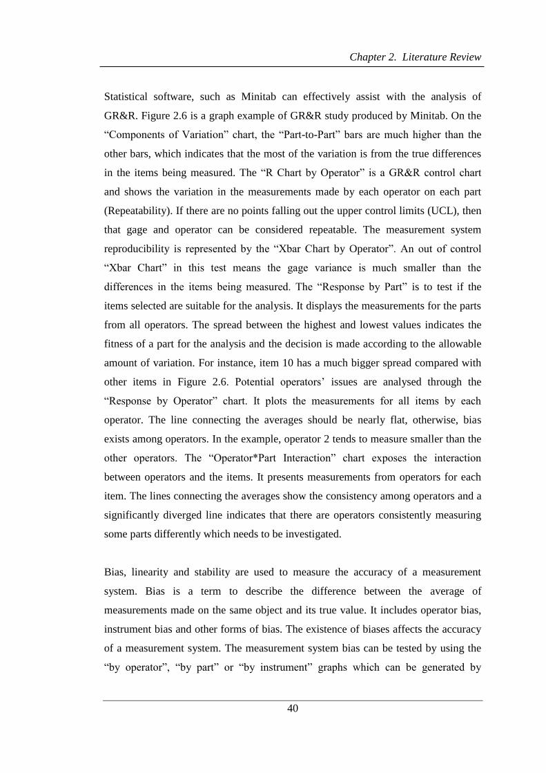
Chapter 2. Literature Review
40
Statistical software, such as Minitab can effectively assist with the analysis of
GR&R. Figure 2.6 is a graph example of GR&R study produced by Minitab. On the
“Components of Variation” chart, the “Part-to-Part” bars are much higher than the
other bars, which indicates that the most of the variation is from the true differences
in the items being measured. The “R Chart by Operator” is a GR&R control chart
and shows the variation in the measurements made by each operator on each part
(Repeatability). If there are no points falling out the upper control limits (UCL), then
that gage and operator can be considered repeatable. The measurement system
reproducibility is represented by the “Xbar Chart by Operator”. An out of control
“Xbar Chart” in this test means the gage variance is much smaller than the
differences in the items being measured. The “Response by Part” is to test if the
items selected are suitable for the analysis. It displays the measurements for the parts
from all operators. The spread between the highest and lowest values indicates the
fitness of a part for the analysis and the decision is made according to the allowable
amount of variation. For instance, item 10 has a much bigger spread compared with
other items in Figure 2.6. Potential operators’ issues are analysed through the
“Response by Operator” chart. It plots the measurements for all items by each
operator. The line connecting the averages should be nearly flat, otherwise, bias
exists among operators. In the example, operator 2 tends to measure smaller than the
other operators. The “Operator*Part Interaction” chart exposes the interaction
between operators and the items. It presents measurements from operators for each
item. The lines connecting the averages show the consistency among operators and a
significantly diverged line indicates that there are operators consistently measuring
some parts differently which needs to be investigated.
Bias, linearity and stability are used to measure the accuracy of a measurement
system. Bias is a term to describe the difference between the average of
measurements made on the same object and its true value. It includes operator bias,
instrument bias and other forms of bias. The existence of biases affects the accuracy
of a measurement system. The measurement system bias can be tested by using the
“by operator”, “by part” or “by instrument” graphs which can be generated by

Chapter 2. Literature Review
41
statistical software, such as Minitab.
Figure 2.6 An example GR&R study through Minitab
Linearity is a measure of the consistency of bias over the range of the measurement
system. Checking linearity requires at least 5 samples that cover the entire range of
the measurement system to be repeatedly measured by the same operator. The
linearity of a measurement system can be analysed by comparing the results from the
test to the reference values. It can also be analysed through linearity plot.
Stability refers to the capability of a measurement system to produce the same values
over time when measuring the same sample. It can be tested through repetitively
measuring a master piece of sample over time and plotting the data on an Xbar chart.
Kappa analysis is a method to perform the MSA for attribute data. It compares the
degree of consensus between appraisers. It is conducted through different appraisers
Perc
ent
Part-to-PartReprodRepeatGage R&R
200
100
0
% Contribution
% Study Var
% Tolerance
Sam
ple
Range
0.10
0.05
0.00
_R=0.0383
UCL=0.1252
LCL=0
1 2 3
Sam
ple
Mean
1.00
0.75
0.50
__X=0.8075UCL=0.8796
LCL=0.7354
1 2 3
Part
10987654321
1.00
0.75
0.50
Operator
321
1.00
0.75
0.50
Part
Avera
ge
10 9 8 7 6 5 4 3 2 1
1.00
0.75
0.50
Operator
1
2
3
Gage name:
Date of study :
Reported by :
Tolerance:
Misc:
Components of Variation
R Chart by Operator
Xbar Chart by Operator
Response by Part
Response by Operator
Operator * Part Interaction
Gage R&R (ANOVA) for Response

Chapter 2. Literature Review
42
making judgements over the same group of parts and the results that are compared
with the expected value from the parts to obtain the Kappa statistic. Kappa statistic is
a coefficient indicating the agreement percentage above the expected agreement by
chance and its value is between 0 and 1.
All the studies in MSA can be performed through statistical software producing both
graphical and statistical analyses.
2.4.5 Control Chart
Control chart which is also known as Shewhart chart, is a statistical-based tool for
monitoring process, a graphical display of changes of a process over time with a set
of rules for determining if a process is in statistical control. It is an important and one
of the most often discussed tools in SPC. In a Six Sigma project, control charts are
often used in the measure and control phases, where in the measure phase, it is used
to distinguish between variations in a process resulting from common causes and
special causes, while in the control phase, to confirm the impact of and test if the
process remains in control after the implementation of solutions. It also helps an
organization and the project teams to monitor the process performance over time to
ensure its stability and enabling predictability. Table 2.10 lists the differences
between common and special causes. There are different types of control charts that
can be used at various situations depending on the data types and sample sizes.
Figure 2.7 summarizes the applications of most commonly used control charts
(George et al., 2005).
In order to create a control chart, the processes need to be closely studied so that
sufficient and representative data can be collected. The steps of constructing a
control chart for a process are as follows:
Determine the data type.
Define the rational subgroups.

Chapter 2. Literature Review
43
Determine sample size, time period and frequency for data collection.
Select the appropriate control chart to be used.
Collect data, construct and analyse the control chart.
Table 2.10 Common causes and special causes
Type of
causes
Definition Typical characteristics
Common
causes
The usual, historical, quantifiable
variation in a system. Process with
only common causes presenting will
run within its normal range
• Expected
• Predictable range of
values
• Purely random
Special causes Unusual, not previously observed,
non-quantifiable variation. Process
with presenting of special causes with
display variation outside what is
expected
• Unexpected
• Unpredictable range of
values
• Not purely random
Figure 2.7 Control charts selection
Data plotted on a control chart is in the time sequence that they occurred. Control
Type of data
Discrete data
Count data
Defects (errors) or nonconformances
Fixed opportunity
c-Chart
Variable opportunity
u-Chart
Binary data
Defective or nonconforming units
Fixed opportunity
np-Chart
Variable opportunity
p-Chart
Continuous data
Subgroup size of 1
ImR
Subgroup size<8-10
Xbar &R
Subgroup size >8-10
Xbar & S
Fixed opportunity: the sample size or “unit” being sampled is constant
Variable opportunity: The sample size or “unite” being sampled changes

Chapter 2. Literature Review
44
charts contain a central line which represents the average of the data and upper and
lower lines stand for the UCL and lower control limits (LCL), respectively. These
lines are determined from the data inputted. The control limits are based upon three
times the standard deviation of the data inputted and therefore are also called 3-
Sigma limits. Because the control limits are calculated from the process data, they
are independent from customer expectations. Figure 2.8 is an example of a control
chart which is statistically in control (within the UCL and LCL). The “measurement”
(vertical axis) on the chart can represent any input or output that needs to be
analysed.
Figure 2.8 A sample control chart
There are eight rules to help the interpretation of control charts for identifying special
causes. These rules assist to locate non-random patterns which indicate that the
process is out of control. The eight standard rules are referred to as Western Electric
Rules (WECO rules), Nelson Rules, AIAG (Automotive Industry Action Group)
Rules, Juran Rules, Hughes Rules, Duncan Rules, Gitlow Rules and Westgard Rules.
These rules supplement the basic rule – one point exceeds the control limits. The
most popular rule is WECO rules and its supplemental rules which are listed below.
1) Points outside one of the 3-sigma control limits (Basic rule).
2) Two of the three consecutive points fall outside and on the same side of the 2-
sigma control limits, but within 3-sigma control limits.

Chapter 2. Literature Review
45
3) Four of the five consecutive points fall outside and on the same side of the 1-
sigma control limits, but within 3-sigma control limits.
4) Eight consecutive points fall on the same side of the centreline.
Supplemental rules:
5) Six points in a row increasing or decreasing.
6) Fifteen points in a row within one sigma.
7) Fourteen points in a row alternating direction.
8) Eight points in a row outside one sigma.
When a special cause exists in a process, corrective actions need to be taken to
address it. Control charts ensure that efforts are made towards the right areas.
Morden data analysis software, such as, Minitab, can help with the creation of
control charts. A process needs to be stable and in control (free from special causes)
before the process capability can be assessed.
2.4.6 Process Capability Analysis (PCA)
The capability of processes can be characterized as the ability of the processes to
provide products or services meeting the required quality criteria in the long term
(Plura et al., 2013). PCA is a measure of performance to evaluate the ability of a
process to satisfy customers (in the form of specifications) (English and Taylor,
1993). PCA is based on the data collected from a process. It compares the inherent
variability of an in-control process to the specification limits (customer
requirements) by using Process Capability Indices (PCIs) which are statistical
indicators of a process capability. The most widely used PCIs are 𝐶𝑝 and 𝐶𝑝𝑘 (Table
2.11). Due to the fact the PICs are not associated with any unit, they can be used to
compare capabilities between different processes. PCA is normally conducted in the
measure phase of a Six Sigma project to present the current performance of a
process, and in control phase as a final capability study to verify the improvement

Chapter 2. Literature Review
46
achieved.
Table 2.11 PCIs – 𝐶𝑝 and 𝐶𝑝𝑘
PCIs Definition Calculation
𝐶𝑝
Process capability ratio - Overall
comparison of process outputs vs.
specification limits
𝐶𝑝 𝑈𝑆𝐿 − 𝐿𝑆𝐿
6𝜎
𝐶𝑝𝑘 Process index - Comparison of variation
against USL and LSL, individually 𝐶𝑝𝑘 𝑀𝑖𝑛 [
𝑈𝑆𝐿 − �̅�
3𝜎 �̅� − 𝐿𝑆𝐿
3𝜎]
�̅� stands for the mean of the data
As a key measure of the process performance, PCA provides a visual representation
through the use of graphs, such as the histogram which also helps to assess and
verify the process capability. Figure 2.9 is a sample PCA through histogram by using
Minitab. The Upper Specification Limit (USL) and Lower Specification limit (LSL)
are determined by customer requirements. Where LSL is preferred to be as minimal
as possible, no LSL figure but a Lower Boundary (LB) is used in constructing the
histogram. The “Within” (solid red line) represents the variation within subgroups,
whereas the “Overall” (dotted line) shows overall standard deviation taking into
account variation from the entire data set and looks at the total process variation.
A PCA normally involves the activities below:
Determine customer requirements (USL and LSL).
Collect process performance data.
Check data normality – If data is normal, standard capability analysis can be
carried out. However, if data is abnormal, it either needs to be normalized or
another special type of capability analysis needs to be utilized.
Generate PCIs and review results.
Computer software, such as Minitab, can assist with the PCA once the data is ready.

Chapter 2. Literature Review
47
Figure 2.9 A sample PCA in histogram generated by using Minitab
2.4.7 Cause and Effect (C&E) Matrix
A C&E matrix is most often used to narrow the number of inputs generated from a
process mapping down to a manageable amount according to their importance to
customers’ priorities. It is a useful tool in the measure phase of a Six Sigma project
to filter the process inputs obtained from process mapping in order to identify the
potential key process inputs that need to be further investigated for improving the
key process outputs (CTQs). The elements of C&E matrix include process inputs and
outputs where the latter are scored by their importance to customers and the former
are scored against the latter.
A C&E matrix can be constructed by:
Identifying key customer requirements (CTQs) which will be the outputs in
the matrix.
Assigning a priority score (1 to 10) to each output according to its importance
to customers.
Identifying process inputs through process mapping and transferring them
onto the matrix.

Chapter 2. Literature Review
48
Rating each input against each output based on the strength of their
relationship using relation scores. Table 2.12 provides a list of relation scores
that are often used in practice.
Obtaining final scores.
Making a decision of the cut-off point in order to select the inputs that need to
be further analysed.
Figure 2.10 provides an example of a C&E matrix.
Table 2.12 Relation scores for C&E matrix
Scores Judgment
0 No relationship
1 Weak relationship
3 Medium relationship
9 Strong relationship
The calculation of the final scores for inputs is as follows:
Suppose there are n outputs and m inputs on a C&E matrix, let 𝑝𝑗 𝑗 1 2 . . . 𝑛
denote the priority score for the jth output, and 𝑟𝑖𝑗 (𝑖 1 2 𝑚 stand for the
relation score for the ith input in relation to the jth output. Then the final score for the
ith input, 𝐹𝑖 can be obtained by using Equation (2.1).
𝐹𝑖 ∑ 𝑟𝑖𝑗𝑛𝑗= × 𝑝𝑗 (2.1)
The C&E matrix produces a reduced list of key process inputs to be further analysed
by other relevant tools. It is worth mentioning that the results produced by a C&E
matrix do not prioritize the inputs but only eliminate unimportant ones.

Chapter 2. Literature Review
49
Figure 2.10 An example of C&E matrix
2.4.8 Failure Mode and Effects Analysis (FMEA)
FMEA is a powerful tool for identifying and assessing potential failures and has been
extensively used in a wide range of contexts. FMEA ranks possible failure modes
based on three criteria: Severity (S), Occurrence (O) and Detection (D) (Table 2.13).
A failure mode is assigned a score against each of these three criteria on an ordinal
scale and a risk priority number (RPN) is then computed for the failure mode by
multiplying the three ordinal scores. FMEA is one of the important methods used in
Six Sigma applications. It can be used in many phases in Six Sigma projects. Table
2.14 provides a list of phases that FMEA can be used in, and its purposes.
FMEA can be conducted through brainstorming by the following steps.
List all process steps/inputs on the FMEA table
Identify all potential failure modes for each step/input
Identify the possible effects for the failure modes and score their severity
Rating of Importance to Customer
7 9 4 10 8 10
Pain
t
thic
kn
ess
Pain
t
hard
nes
s
Rate
Co
vera
ge
Su
rfac
e
qu
ality
Pro
pe
r
sch
em
e
Total
Process Input
Surface contamination 1 3 3 9 9 0 208
Surface roughness 0 1 3 3 9 0 123
Air pressure 9 1 9 9 9 0 270
Lot number 1 3 0 3 1 3 102
Nozzle type 9 0 3 9 9 0 237
Primer age 9 9 9 3 9 0 282
Ambient temp 1 3 9 0 3 0 94
Relative humidity 1 9 9 1 9 0 206
Surface contamination 1 9 3 9 9 1 272
Priority scores
CTQs
Relation scores
Final scores

Chapter 2. Literature Review
50
Identify the causes of those failure modes and rate their occurrence
Identify any control in place to detect the issue and score the likelihood of
detection
Obtain RPN, rank all inputs and identify critical inputs that need to be
addressed
Table 2.13 Explanation of Severity, Occurrence and Detection in FMEA
Description The lowest
score (1)
The highest
score (10)
Severity severity of the potential effects of the
failure on customers (both internal and
external)
Low impact High impact
Occurrence Probability that a failure can occur
during the expected lifetime of the
product or service
Not likely to
occur
Very likely to
occur
Detection Probability that the problem will be
undetected before it reaches the end-
user/customer
Very likely to
be detected
Not likely to be
detected
Table 2.14 FMEA applications in Six Sigma phases
Phase Purpose
Measure Failure prioritization – Identify and prioritize critical inputs
associated causes of failures that need to addressed and
Analysis Help to address where to look for root causes
Improve Test solution and identify potential risks
Control Monitor performance and enhance process
Table 2.15 is a sample FMEA form with explanation of its contents. Involving the
right people has proven to be a key element in the successful application of FMEA.
The team should include those that have good understanding of the process and can
contribute to the identification of failures, such as process owners.
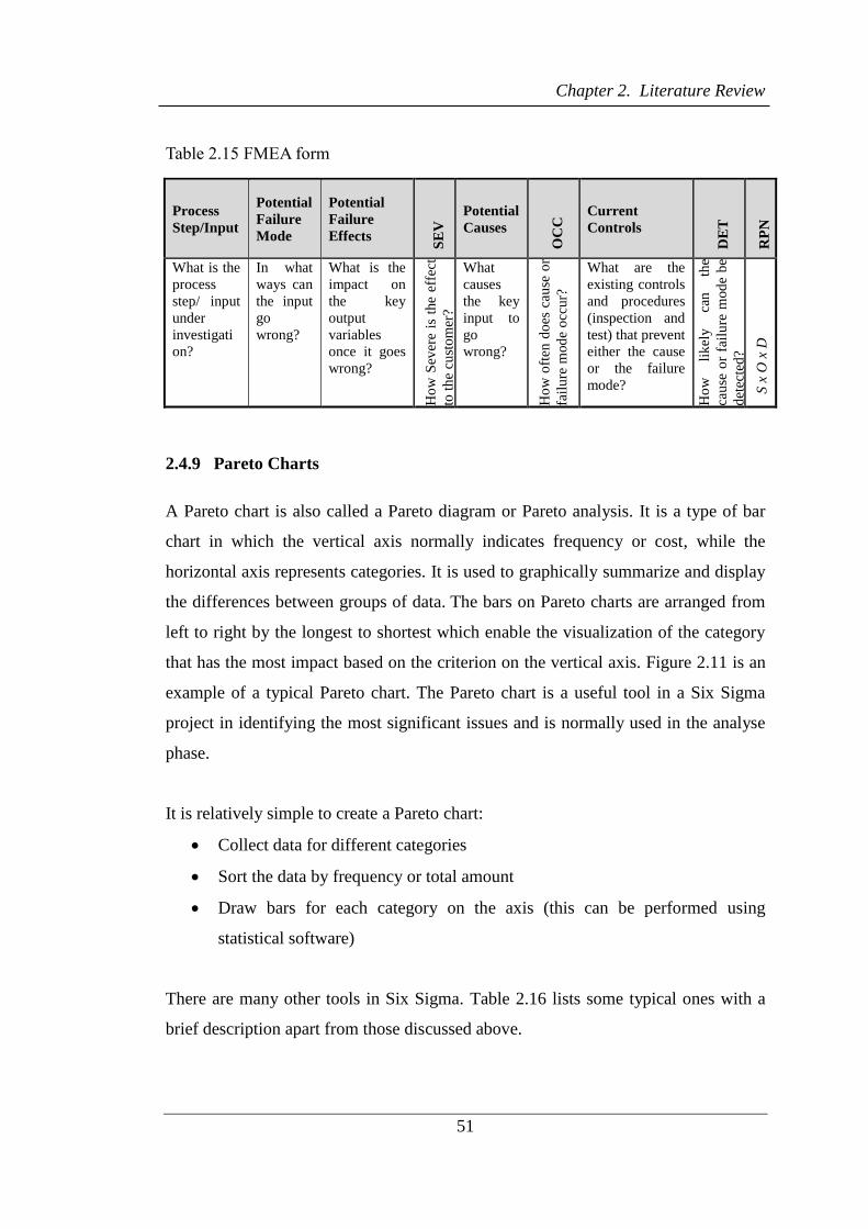
Chapter 2. Literature Review
51
Table 2.15 FMEA form
Process
Step/Input
Potential
Failure
Mode
Potential
Failure
Effects
SE
V Potential
Causes
OC
C Current
Controls
DE
T
RP
N
What is the
process
step/ input
under
investigati
on?
In what
ways can
the input
go
wrong?
What is the
impact on
the key
output
variables
once it goes
wrong?
Ho
w S
ever
e is
the
effe
ct
to t
he
cust
om
er?
What
causes
the key
input to
go
wrong?
Ho
w o
ften
do
es c
ause
or
fail
ure
mod
e o
ccur?
What are the
existing controls
and procedures
(inspection and
test) that prevent
either the cause
or the failure
mode?
Ho
w
lik
ely
ca
n
the
cau
se o
r fa
ilu
re m
od
e b
e
det
ecte
d?
S x
O x
D
2.4.9 Pareto Charts
A Pareto chart is also called a Pareto diagram or Pareto analysis. It is a type of bar
chart in which the vertical axis normally indicates frequency or cost, while the
horizontal axis represents categories. It is used to graphically summarize and display
the differences between groups of data. The bars on Pareto charts are arranged from
left to right by the longest to shortest which enable the visualization of the category
that has the most impact based on the criterion on the vertical axis. Figure 2.11 is an
example of a typical Pareto chart. The Pareto chart is a useful tool in a Six Sigma
project in identifying the most significant issues and is normally used in the analyse
phase.
It is relatively simple to create a Pareto chart:
Collect data for different categories
Sort the data by frequency or total amount
Draw bars for each category on the axis (this can be performed using
statistical software)
There are many other tools in Six Sigma. Table 2.16 lists some typical ones with a
brief description apart from those discussed above.

Chapter 2. Literature Review
52
Figure 2.11 An example of typical Pareto chart
.
Table 2.16 Useful tools in Six Sigma projects
Tools Phase Description
Affinity diagrams Any
phase
An effective tool to organise ideas, opinions and issues
into natural groups or themes.
Cause and effect
diagrams (fishbone or
Ishikawa diagrams)
Analyse A tool to display all potential causes of a problem and
help to uncover the root causes.
Hypothesis Testing Analyse
It uses a variety of statistical analyses to determine if
any statistically significant difference among the
observed relationship between two or more samples
can be explained by random chance alone. Figure
2.12 lists the tests to choose in accordance with the
data types.
Design of Experiments
(DOE) Improve
A powerful tool to analyse and identify the factors that
have key influence on a process and optimise them
through a variety of experimental situations.
Poka Yoke (Mistake
proofing) Improve
A method to ensure that human error is avoided in the
future, or to make it impossible to make an error.
Pugh Matrix Improve
A tool to compare and rank different concepts and help
to arrive at an optimum that may be a hybrid or variant
of others.
Control plan Control
A document containing details of inspection points in a
process and responsibility for each activity to ensure
the sustainability of a process improvement in the long
run.

Chapter 2. Literature Review
53
Input Xs
Ou
tpu
t Y
(si
ng
le)
Single X
Multiple X
Discrete Continuous
Discrete Continuous
Dis
cret
e
Chi-Square Logistic
Regression
Dis
cret
e
Multiple
Logistic
Regression
Multiple Logistic
Regression
Co
nti
nu
ou
s
ANOVA
Means/
Medians Tests
Correlation &
Regression
Co
nti
nu
ou
s
ANOVA
Medians Tests
Multiple
Regression
Figure 2.12 Hypothesis testing road map
The application of tools is only one part of the Six Sigma process which alone will
not secure the success of Six Sigma implementation. It works best in an environment
with the top management support, effective training and the fulfilment of other CSFs
during the Six Sigma implementation
2.5 Six Sigma in the Service Industries
Service industries have raised their awareness of meeting customer needs while
remaining economically competitive with increasing market competition and
customer expectation. However, research shows that the COPQ (rework, mistakes,
and abandoned projects, etc.) in service-based businesses and processes typically run
as high as 50 percent of the total budget (Pande et al., 2000). Thus, how to improve
service quality has become a crucial issue in today’s service industries.
Although Six Sigma was originally developed for manufacturing processes,
traditional manufacturing companies are taking their Six Sigma experiences and
moving them to their service operations. For example, the Ford Motor Company has
achieved cost savings from successfully applying Six Sigma in its corporate real
estate group, facility management and maintenance functions (Holtz and Campbell,
2004). Today service firms and service functions within many sectors are using Six

Chapter 2. Literature Review
54
Sigma to improve their profits and performance. Six-Sigma is particularly attractive
to the service sector due to its customer-driven methodology (Tagahaboni-Dutta and
Moreland, 2004). It offers a disciplined approach to improve service effectiveness
(i.e. meeting the desirable attributes of a service) and service efficiency (i.e. time and
costs) (Antony, 2004a) leading to improved customer satisfaction. According to the
survey conducted by DynCorp, 38.2% of the companies in the US with a Six-Sigma
programme in place were service companies (Mekong Capital Ltd., 2004). A large
number of examples of successful applications of Six Sigma in the service industries
have been documented. For example, in the financial service sector, BOA applied
Six Sigma to reduce defects in operations, cut unnecessary costs, improve efficiency
and achieve a higher customer satisfaction level. Four years from its application in
2001, Six Sigma helped BOA to achieve two billion dollars in revenue gains and cost
savings. Apart from BOA, American Express, GE Capital Corp., JP Morgan Chase,
SunTrust Banks, HSBC and Citibank have all seen significant improvements in
various sections through the implementation of Six Sigma projects. In the healthcare
sector, Six sigma helped Commonwealth Health Corp., Thibodaux Regional Medical
Centre, Good Samaritan Hospital and many more to achieve cost savings and
improve quality of service.
Service industries are even more in need of Six Sigma than manufacturing due to the
fact that the outputs tend to go directly to customers whereas in manufacturing most
defects are either scrapped or fixed before shipping (Tennant, 2001). However, the
implementation of Six Sigma in service industries has its difficulties. Six Sigma is
known as a fact-based method, in other words, statistically-based. The products of
service industries are normally intangible and involve direct customer
communication and participation. They tend to have less measurable process with
non-standard outputs and are not quantitatively oriented as manufactured products.
The products of service industries are often consumed at the same time as they are
produced and are highly variable depending on the service providers, which leads to
more errors and higher variation. Therefore, lack of qualified data for decision
making is a common issue which leads to difficulties in Six Sigma applications in the
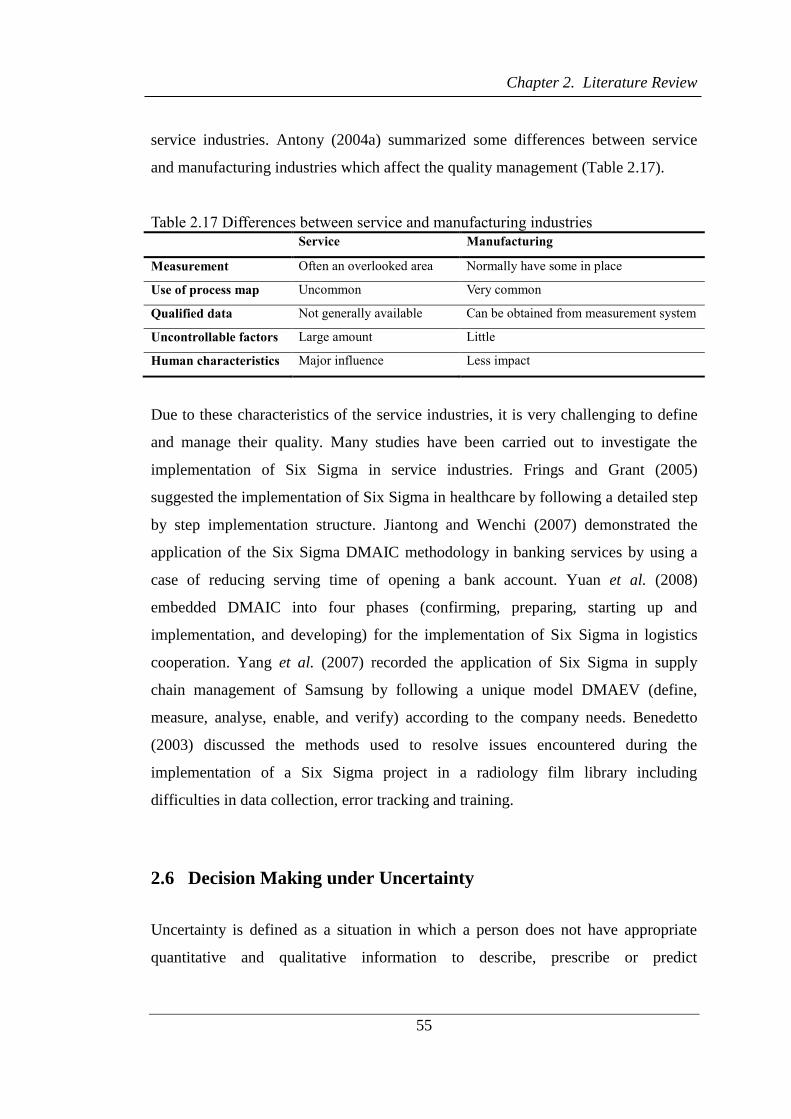
Chapter 2. Literature Review
55
service industries. Antony (2004a) summarized some differences between service
and manufacturing industries which affect the quality management (Table 2.17).
Table 2.17 Differences between service and manufacturing industries
Service Manufacturing
Measurement Often an overlooked area Normally have some in place
Use of process map Uncommon Very common
Qualified data Not generally available Can be obtained from measurement system
Uncontrollable factors Large amount Little
Human characteristics Major influence Less impact
Due to these characteristics of the service industries, it is very challenging to define
and manage their quality. Many studies have been carried out to investigate the
implementation of Six Sigma in service industries. Frings and Grant (2005)
suggested the implementation of Six Sigma in healthcare by following a detailed step
by step implementation structure. Jiantong and Wenchi (2007) demonstrated the
application of the Six Sigma DMAIC methodology in banking services by using a
case of reducing serving time of opening a bank account. Yuan et al. (2008)
embedded DMAIC into four phases (confirming, preparing, starting up and
implementation, and developing) for the implementation of Six Sigma in logistics
cooperation. Yang et al. (2007) recorded the application of Six Sigma in supply
chain management of Samsung by following a unique model DMAEV (define,
measure, analyse, enable, and verify) according to the company needs. Benedetto
(2003) discussed the methods used to resolve issues encountered during the
implementation of a Six Sigma project in a radiology film library including
difficulties in data collection, error tracking and training.
2.6 Decision Making under Uncertainty
Uncertainty is defined as a situation in which a person does not have appropriate
quantitative and qualitative information to describe, prescribe or predict

Chapter 2. Literature Review
56
deterministically and numerically a system, its behaviour or other characteristics
(Zimmermann, 2000). Uncertainty in principle is originated from failures,
assumptions, consequence methodologies, unavailability or incompleteness of data.
Characteristics of OSFs of shipping companies render themselves a high level of
uncertainty which affects the implementation of Six Sigma. Due to the large
involvement of human activities in the operations, experts’ subjective judgements are
often used in order to obtain valid data. Numbers offer precision in scientific
communication and efficiency of aggregation and manipulation, but their
characterization of a person’s experiences is usually far more impoverished than his
or her words (Stiles, 1993). Effective handling of uncertainties and using of
qualitative data can improve the applicability and accuracy of Six Sigma and
increase its applicability in an environment where high uncertainties exist.
The implementation of Six Sigma in OSFs of shipping companies therefore needs to
appropriately tackle the uncertainties inherently involved in the different steps of the
DMAIC methodology. Many tasks such as project selection, fault measurement and
failure analysis, KPI control and improvement, are essentially processes of multiple
criterion decision making (MCDM) under uncertainty, requiring analysts to derive
rational decisions from uncertain and incomplete data contained in different
quantitative and qualitative forms. Typical MCDM problems are addressed through
several crucial steps such as criteria selection, criteria importance analysis,
alternative identification and evaluation. Well-established MCDM methodologies are
therefore reviewed with respect to the steps in order to provide a holistic knowledge
base on their applications in the context of shipping and maritime sectors. However,
it is noteworthy that none of them is considered suitable under all MCDM
environments and therefore hybrid approaches are often developed to deal with
complex scenarios involving different types of uncertainties.
Strengths, Weaknesses, Opportunities and Threats (SWOT) analysis has its mutual
origins in the work of business policy academics at Harvard Business School and

Chapter 2. Literature Review
57
other American business schools from the 1960s onwards. The work of Andrews
(1971) has been especially influential in popularizing the idea that a good strategy
means ensuring a fit between the external situation a firm faces (threats and
opportunities) and its own internal qualities or characteristics (strengths and
weaknesses) (Hill and Westbrook, 1997). The applications of the SWOT analysis to
select criteria in a multi-criteria situation have invariably been combined with AHP
and/or TOPSIS (Arslan and Turan, 2009; Notteboom, 2011; Kandakoglu et al., 2009;
Celik and Kandakoglu, 2012), in which SWOT is often used to examine and
determine the criteria while AHP is utilised to assign the priority of each criterion
and to rank the alternatives. TOPSIS is sometimes used to replace AHP in the
process of ranking the alternatives. For instance, the combination of SWOT analysis,
AHP and TOPSIS has been used to aid ship owners to choose the suitable shipping
registry (Kandakoglu et al., 2009). Furthermore, it has been seen that SERVQUAL
(Kannan et al., 2010) and Exploratory Factor Analysis (EFA) (Spearman, 1904;
Fabrigar et al., 1999) are used to select criteria in shipping. Kannan et al. (2010)
proposed a framework based on AHP and SERVQUAL for benchmarking service
quality of container shipping companies, while Chao and Lin (2011) combined EFA
and fuzzy AHP for a two-phased method of evaluating advanced quay cranes in
container terminals (Puttich, 2013).
AHP, as one of most widely used MDCM approaches, is capable of assisting criteria
selection, criteria importance analysis and alternative evaluation. The best decision
can be made when qualitative and quantitative aspects of a decision are included
(Saaty, 1990). AHP uses the concept of pair-wise comparison to improve the
efficiency of synthesising qualitative and quantitative evaluations in a decision
process. It consists of four steps of establishing the hierarchy of criteria, making pair-
wise comparison of the criteria and alternatives, estimating the weights of the criteria
and the relative performance values of the alternatives with respect to each criterion,
and aggregating the weights and performance values for alternative priority. The
visibility and easiness characteristics of AHP contribute to its popularity in research
projects across different industries. Vaidya and Kumar (2006) revealed that the AHP

Chapter 2. Literature Review
58
method is used in nearly 150 applications. Several examples are presented to
demonstrate the AHP applications in the shipping and maritime sectors. AHP has
been widely used in port choice and competitiveness evaluation (Lam and Dai,
2012; Yeo et al., 2010; Yeo et al., 2014) as well as in vessel selection (Yang et al.,
2009b; Xie et al., 2008). Carlos Perez-Mesa et al. (2012) determined optimal
allocation of ports between land and intermodal transport, taking into account
environmental externalities. AHP has also been used to investigate the human
reliability of ship operations (Ung et al., 2006), design support evaluation for the
offshore industry (Sii and Wang, 2003), selection of Nigerian ports regarding service
quality (Ugboma et al., 2004), and maritime regulation implementation by
Karahalios et al. (2011).
The AHP has some advantages over other methods because of its simplicity and its
ability to rank parts of a multi-criteria problem in a hierarchical structure (Chen and
Lin, 2006). However it lacks the ability to model the interdependencies among the
criteria, which constrains its applications in large engineering and management
systems. Analytical Network Process (ANP) (Saaty, 1990) was developed to
complement the AHP in a way that the criteria are presented in a network (instead of
hierarchy) structure. Although showing some attractiveness in modelling
interrelationship among the criteria, ANP still reveals some practical problems in its
real applications. For instance, to construct the associated supermatrix ANP requires
too much pair-wise comparison input information, which is often difficult to obtain
using simple questionnaires. As a result, new methods are developed to seek for
alternative solutions to weight distribution of the criteria in a network organisation.
The hybrid of DEMATAL and ANP (D-ANP) (Chen, 2012; Vujanovic et al., 2012;
Tsai and Hsu, 2010; Lee et al., 2011) or DEMATEL and AHP (D-AHP) (Dalalah et
al., 2011) is among the most popular in the relevant literature. The difference
between D-ANP and D-AHP lies in that the former is to use the qualitative analysis
of DEMATAL for identifying the criteria having interdependencies (and ignoring
independent criteria), which can help simplify the requirements of input information
in construction of supermatrix in ANP. The latter directly combines the result from

Chapter 2. Literature Review
59
the quantitative analysis of DEMATEL with the one from the AHP. By doing so, the
weight of a criterion can be presented in terms of both its influence to the other
criteria (through DEMATEL) and its relative importance in decision making
(through AHP). Compared to the criteria weights assigned by subjective experts,
another factor used to rationalise the weights is considered based on the objective
information on performance evaluation of each alternative against the same criterion
through entropy calculation. Entropy results are often combined with the ones from
AHP in MCDM analysis (Yang et al., 2009c; Chou and Liang, 2001).
Evaluating decision alternatives in a real-world scenario is a complex process as it
frequently involves uncertainty in data. Complexity in MCDM is consequently
caused by the rational handling of qualitative criteria and uncertain or missing
information (Yang and Xu, 2002b). Such uncertainties are broadly categorized as
fuzziness, incompleteness and randomness (Liu et al., 2004). Fuzzy logic (Zadeh,
1965), ER (Yang and Xu, 2002b) based on Dempster-Shafer theory (Dempster,
1967; Shafer, 1976) and Bayesian network (BN) based on Bayesian probabilistic
theory (Jensen, 2001) are used to tackle the three types of uncertainty respectively.
Fuzzy logic is a superset of conventional Boolean logic with extensions to account
for imprecise information. Fuzzy logic permits vague information, knowledge and
concepts to be used in an exact mathematical manner. Linguistic variables such as
“definite”, “likely”, “average”, “unlikely” and “impossible” are necessary media
used to describe continuous and overlapping states. This enables qualitative and
imprecise reasoning statements to be incorporated with fuzzy algorithms or fuzzy
rule bases producing simpler, more intuitive and better-behaved models. Fuzzy logic
is based on the principle that every crisp value belongs to all relevant fuzzy sets to
various extents, called the degrees of membership. Pure fuzzy logic has extremely
limited applications in business (the only popularised application is the Sony
Palmtop) and the main use of fuzzy logic is as an underlying logic system for fuzzy
expert decision making systems (Pai et al., 2003). Fuzzy logic has been successfully
applied for a wide range of single and MCDM problems. For instance, Chou (2010)

Chapter 2. Literature Review
60
proposes a fuzzy MCDM methodology for solving the container transhipment hub
port selection dilemma under fuzzy environment. Wang and Lee (2010) utilise a
fuzzy MCDM method for evaluating the financial performance of container shipping
companies based on extended fuzzy preference relation and using linguistic weights.
The application of fuzzy logic in MCDM becomes more compelling when being
combined with AHP, (Bulut et al., 2012; Hsu, 2012; Chao and Lin, 2011), TOPSIS
(e.g. (Yeh and Chang, 2009; Durbach and Stewart, 2012; Yang and Wang, 2013;
Kannan et al., 2014), and PROMETHEE (e.g. (Shirinfar and Haleh, 2011; Gupta et
al., 2012; Tavakoli et al., 2013)
The theory of evidence was first generated by Dempster (1967) and further
developed by Shafer (1976). The Dempster-Shafer theory of evidence or D-S theory
was originally used for information aggregation in expert systems as an approximate
reasoning tool (Buchanan and Shortliffe, 1984; Mantaras, 1990) and then used in
decision making under uncertainty and risk in contrast to Bayes decision theory
(Yager, 1992; Yager, 1995). ER is developed on the basis of the D-S theory. The use
of ER as a decision making tool has been widely reported in the literature. An
important achievement of applying ER to decision analysis is to incorporate it into
traditional MCDM methods for addressing the degree of belief associated with
subjective judgements. The lack of data, the inability of assessors to provide precise
judgements, or the failures of some assessors to provide judgements in group
decision-making can result in an incomplete assessment (Yang and Xu, 2002b). An
ER based decision making approach for MCDM problems with both qualitative and
quantitative criteria under uncertainty was developed in the early 1990’s (Yang and
Singh, 1994; Yang and Sen, 1994). The kernel of such an approach is an ER
algorithm, which was generated by Yang and Singh (1994), later updated by Yang
and Sen (1994) and further modified by Yang (2001) and Yang and Xu (2002b). ER
is applied for ranking alternatives or selecting the best compromise alternative in a
process, in which both quantitative and qualitative attributes are simultaneously
satisfied as much as possible (Yang and Singh, 1994). Several applications of this
approach are addressed in the maritime related literature (Yang, 2001; Sii et al., 2001;

Chapter 2. Literature Review
61
Yang et al., 2005; Yang et al., 2009c; Yang et al., 2014).
A BN (also called belief network, or probabilistic network) is a graphical
presentation of probability combined with a mathematical inference calculation. It
can be used to represent dependencies between decision variables. Each variable
represented as a node, is connected by directed links, represented as arrows or arcs,
with conditional probability table (CPT) values assigned to the variables making up a
BN (Jensen, 2001). The graphical representation makes BNs a flexible tool for
constructing the models of causal impact between events, in particular when the
causal impact has a random nature. A BN serves as a model for a part of the world
and the relations in the model reflect causal impact between events. The reason for
building these models is to use them when making decisions under a dynamic
environment. In other words, the probabilities provided by the network are used to
deal with the dynamic changes of variables and support some kind of decision
making involving randomness.
It is possible to decompose multi-attribute/criteria utility functions in a similar way: a
node is created to represent the attribute of interest, which has as its parents all the
other attributes on which it depends. Furthermore, the utility node(s) will be created
to have decision/deterministic and chance node(s) as parents, since the utility
depends both on the state of the world and the actions performed by decision makers.
The resulting graph is called an influence diagram (ID). The utility functions allow
IDs to incorporate the notation of preference, which is necessary to wider decisions
with multiple attributes. The precedence links attached in the diagrams make it
possible to take decisions or perform actions in a sequential order. An ID was
originally developed to substitute conventional decision trees in modelling and
solving real world symmetric decision problems. An ID is solved by computing a
strategy yielding the highest expected utility (Yang, 2006). In the framework of IDs,
Gupta et al. (2012) provided a natural representation for capturing the semantics of
decision making with a minimum of clutter and confusion for decision makers
(Shachter and Peot, 1992) and offerd comparative advantages of easy numerical

Chapter 2. Literature Review
62
assessment and effective representation of independencies between variables over
trees. These factors contributed to the widespread use of IDs as a tool for
representing and analysing complex decision problems in recent years (Fenton and
Neil, 2001; Willems et al., 2005; Diehl and Haimes, 2004; Delcroix et al., 2013;
Yang et al., 2009a).
In shipping quality control, linguistic terms exist together with numbers. Therefore,
methods adopted for qualitative analysis in this study need the capability of handling
both quantitative and qualitative data by investigating the aforementioned methods,
models, theories and their combinations.
2.7 Discussion
Globalization exposed companies to an increasing market competition. Quality
control has therefore become an increasingly attractive topic to both academics and
practitioners. During the evolvement of SPC, different methods have been created,
tested, discussed and criticized. Many of them have faded away for different reasons.
Six Sigma, as an effective quality improvement methodology, is the most eye-
catching method in today’s quality control. It has been successfully implemented in
many industries, including the service industry, to improve business performance and
the benefits achieved have been well documented. The tools in Six Sigma are not
newly created, but the principle of Six Sigma and the logical integration of those
tools have made Six Sigma outperform the other quality control methods.
To enjoy the benefits that Six Sigma could bring to shipping, the existence of
uncertainty needs to be carefully addressed by OSFs of shipping companies. The
current methods in Six Sigma are inadequate in dealing with uncertainties. This
chapter has reviewed some of the uncertainty treatment methods in detail which will
be employed to improve the capability of Six Sigma tools so that they can be
effectively and confidently used in OSFs.

Chapter 3. A Modified Six Sigma Methodology for OSFs of Shipping Companies
63
Chapter 3. A Modified Six Sigma Methodology for OSFs
of Shipping Companies
3.1 Introduction
Shipping is in its nature a service industry providing transportation. Quality,
efficiency and safety are major factors in determining the success of a shipping
company in an ever changing dynamic environment. Under today’s global market
competition, shipping, as a highly globalized industry, is constantly seeking ways to
improve its competitiveness and maintain/increase its profitability. Owners are
managing a large bundle of associated services for the clients to enable and support
shipping operations. The quality of these services has been recognized as an essential
part in meeting customers’ satisfaction level. Six Sigma, as a statistically-based
quality improvement methodology, has been successfully implemented in many
industries to improve business performance, but not in shipping in general, or
onshore service in particular, largely due to the unavailability and incompleteness of
relevant data. This chapter aims at proposing a revised framework to implement Six
Sigma in the OSFs of shipping companies to realize a more visible process that can
be effectively measured, monitored and improved so as to better meet customer
requirements. Through its implementation in a real test case in a world leading
shipping line, the new framework demonstrates its feasibility in practice as well as its
advance in facilitating quality improvement and cost saving in shipping operations
particularly in the troughs of shipping cycles such as economic crisis.
3.2 The Needs of Six Sigma in the OSFs of Shipping Companies
Yilmaz and Chatterjee (2000) found that most service processes such as shipping,
invoicing, billing, payroll, customer order entry, etc. are performing at a quality level

Chapter 3. A Modified Six Sigma Methodology for OSFs of Shipping Companies
64
of less than a 3.5 sigma, with a defect rate of over 23,000 ppm or 97.7 per cent yield.
OSFs of shipping companies contain most of these functions mentioned and more.
According to GE's 1996 annual report, it has been estimated that less than the Six
Sigma quality, i.e., the three-to-four Sigma levels that are average for most U.S.
companies, can cost a company as much as 10-15% of its revenues. A slight
improvement on the Sigma level could dramatically reduce the number of defects
and result in not only financial returns, but also higher customer satisfaction and
loyalty. Research has suggested that it is more profitable to retain customers in the
long term and that a 5% increase in customer loyalty can produce profit increases
from 25% to 85% (Reichheld and Sasser, 1990). The top of the list of customer
suggestions for improving shipping line performance includes “Advance notice of
shipping delays”, “Better trained / knowledgeable staff”, “More cooperative”,
“Speedy document release”, “Closer monitoring” and “Faster service/procedures”
(Srinivas Durvasula et al., 2002). It presents a need for improving service quality of
OSFs in shipping companies. Antony (2004a) listed several benefits of applying Six
Sigma in the service industries including fact based decision making, better
understanding of customer needs, reliable and efficient operation, improved
employee satisfaction, more stable performance, proactive company culture and
improved cross-function teamwork. All of them will benefit the OSFs to improve
their performance and better meet customer expectations.
In service industries, including the shipping sector, qualitative data is equally if not
more important compared to quantitative data. Due to the lack of qualified
quantitative data and the existence of uncertainties, subjective judgements are
frequently needed to obtain information. There are no structured qualitative methods
in the Six Sigma methodology to effectively deal with qualitative information. The
current analytical tools in Six Sigma applications are mostly based on the use of
quantitative data and require the transformation of qualitative data into quantitative
data. This has limited the application of Six Sigma tools in an environment in which
the uncertainty in data is high.

Chapter 3. A Modified Six Sigma Methodology for OSFs of Shipping Companies
65
3.3 A Modified Six Sigma Methodology
OSFs of shipping companies have unique characteristics, which are human intensive,
directly customer interactive, a large number of cross-department activities and
evolving processes.
The traditional Six Sigma uses DMAIC as standard methodology (section 2.3.4).
Although the importance of preparation and recognition have been recognized by
many researchers and practitioners, in practice, they are often neglected or not well
conducted by simply following the DMAIC methodology, which will compromise
the project results. A newly modified framework of implementing Six Sigma,
capable of modelling the quality control in OSFs of shipping companies, P-DMAIC-
R, is proposed and presented in Figure 3.1 by taking into consideration the above
issue and the features of shipping companies.
3.3.1 Top Management Support / Involvement
Suggested as the top CSF in the successful implementation of Six Sigma, top
management support / involvement is a critical element in the success of Six Sigma.
It is essential in ensuring the project is in line with the company strategy, securing
sufficient resources, keeping motivation and removing barriers during the
implementation process. Six Sigma’s success demands the full support and personal
involvement from the highest executive. According to an associate dean and
professor of operations and manufacturing management at the John M. Olin School
of Business, “The top executive must be part of Six Sigma (Andersen et al.), must
change the agenda of upper management meetings so the quality initiative is right
near the top'' (Henderson and Evans, 2000). The success of Six Sigma lies in the
commitment of top management and should only be initialized once the managers’
commitments are fully established. This is especially important in OSFs of shipping
companies where human activities are heavily involved in every part of the operation
processes.

Chapter 3. A Modified Six Sigma Methodology for OSFs of Shipping Companies
66
Figure 3.1 Framework of implementing Six Sigma in OSFs of shipping companies
3.3.2 Prepare
DMAIC has been widely accepted as the methodology for Six Sigma. Although
project selection, team member selection and belt training have been recognized as
important elements in Six Sigma applications, they are not being built into the
standard methodology framework. They are indispensable for the successful
implementation of Six Sigma in OSFs of shipping companies and therefore are
structured into the framework as a new stage of the standard methodology, namely
Con
tin
uou
s m
an
agem
ent
sup
port
, in
volv
emen
t an
d c
om
mu
nic
ati
on
Pre
par
e
Project selection
Team member selection
Team/Belts training
Define Measure Analyse Improve Control
D
efin
e cu
stom
er r
equir
emen
ts
S
et i
nit
ial
goal
s
Mak
e a
pla
n
P
repar
e p
roje
ct c
har
ter
M
ap p
roce
ss
D
evel
op m
easu
rem
ent
pla
n
C
oll
ect
dat
a
Mea
sure
curr
ent
per
form
ance
A
nal
yse
dat
a an
d i
den
tify
core
ca
use
s of
def
ects
Det
erm
ine
impro
vem
ent
targ
et
D
esig
n s
olu
tions
P
erfo
rm c
ost
ben
efit
anal
ysi
s
Imple
men
t so
luti
ons
D
evel
op s
tandar
ds
and
pro
cedure
s
Est
abli
sh s
tandar
d m
easu
res
to
mai
nta
in p
erfo
rman
ce
V
erif
y b
enef
its
achie
ved
Recognize contribution and success

Chapter 3. A Modified Six Sigma Methodology for OSFs of Shipping Companies
67
“prepare” (Figure 3.1).
Project selection
Six Sigma is a project-driven approach and an organisation can achieve the strategic
goal through effectively accomplishing projects. Selecting the right project is one of
the most critical CSFs for the effective deployment of a Six Sigma programme.
Project selection is a process of evaluating individual projects to choose the one or
ones that can meet organizations’ current objectives. Literature has revealed that
project selection is the most critical and mostly mishandled activity in the launching
of Six Sigma (Pande et al., 2000). A right project is the one that can be completed
within a reasonable time and delivers tangible benefits that the organization requires
(such as, reducing cost or improving customer satisfaction). It is a multi-criteria
decision making process which requires assessment of different criteria in a project
selection process. Antony (2004b) pointed out that the prioritisation of projects in
many organisations is still based on pure subjective judgement. Very few powerful
tools are available for prioritising projects. Many studies have been conducted in
project selection for Six Sigma projects (Kumar et al., 2007; Su and Chou, 2008;
Kumar et al., 2009; Buyukozkan and Ozturkcan, 2010). However, the project
selection process will be very challenging when the data used to describe the
selection criteria is presented in various forms and effective data collection,
transformation and aggregation become necessary. The selection process is normally
conducted under the guidance of experienced Six Sigma practitioners, by personnel,
normally senior managers, who have a good understanding and control over
company objectives, finance requirements and resources allocation.
Team selection and training
Properly defined roles can facilitate a smooth Six Sigma implementation by
providing a clear understanding of the responsibilities and accountabilities to the
personnel involved. Six Sigma implementation involves a belt system which contains
a dedicated Champion / Sponsor at the senior management level of the organisation,

Chapter 3. A Modified Six Sigma Methodology for OSFs of Shipping Companies
68
MBB for providing training courses, BBs as full time improvement experts, GBs
among supervisors and other team members from operators and front-line staff
(Magnusson et al., 2003). Table 3.1 provides an overview of the Six Sigma belt
system.
A comprehensive training package needs to be provided to team leaders. There are
different organizations in the market that can provide external training. A company
can also hire qualified MBBs to provide training internally. The differences of
internal and external trainings are listed in Table 3.2. Effective training of BBs and
any other Six Sigma project leaders is not limited to the knowledge of Six Sigma
tools, but also project management and people skills, such as team collaboration.
Table 3.1 Six Sigma belt system
Roles Position Main Responsibilities
Champion / Sponsor Member of senior
management team
Driver of a project
Set broad goals
Scope project
Secure resources, remove barriers,
advocate progress and achievement
MBB Full time experts Trainer and coach
Provide Six Sigma trainings
Work as agent of change
Coach BB and GB
BB Full time resource from the
very best leaders
Project Manager / Trainer
Develop and maintain project charter
and schedule
Select team members
Define and assist team members in
using Six Sigma tools
GB Middle management,
supervisors
Project Manager / team member
Implement project by using tools and
methodologies
Other team members
Operators Provide information base on
experience to support the
measurement, analysis and
improvement

Chapter 3. A Modified Six Sigma Methodology for OSFs of Shipping Companies
69
3.3.3 DMAIC
DMAIC provides a consistent approach for organizations in implementing Six
Sigma. It emphasises “customer needs” and “continuous measurement” to achieve
improvement on current processes which are essential aspects in shipping company
quality improvement. It also offers the opportunity to redesign the processes if it
becomes necessary. Therefore, DMAIC can make an effective model in Six Sigma
implementation used in OSFs of shipping companies.
Table 3.2 Key characteristics associated with internal versus external training
(Kubiak, 2012)
Internal training External training
Less expensive Can be very expensive
Takes time to develop course material
A variety of courses can be delivered
almost at a moment's notice
Requires that a certain number of high-
level belts be on board to develop the
material
Does not require high-level belts to be on
board
Consistency of material content likely to
degrade with large, decentralized
organizations Consistent material content
Future instructors can pair with current
instructors for training
The development of internal instructors is
unclear
Deployment paced by the rate instructors
is developed
Instructors usually available almost at
moment's notice
The “define” phase provides a top level project definition / charter with goals and
plans. In this phase, “defect” in the process is defined and the COPQ is calculated to
provide baseline data. The COPQ includes the costs of internal failures, external
failures, appraisal (prediction, audit and detection) and prevention. They are the costs
that would disappear if every task were continuously performed without deficiency

Chapter 3. A Modified Six Sigma Methodology for OSFs of Shipping Companies
70
every time and can be varied for different function areas or companies. Figure 3.2
presents an example of COPQ that may exist in a company. COPQ creates a burning
platform as well as helps an organisation to identify areas that have direct bearing on
profitability. Once the COPQ is identified, an aggressive but realistic goal needs to
be set based on the CTQs. A realistic project plan/tracker with detailed breakdown
of milestones is also developed in this phase. These are the major elements of a
project charter which need to be reviewed and updated throughout the project
implementation.
Figure 3.2 Example of Cost of Poor Quality
The objective of the “measure” phase is to collect data for measuring the current
performance output (Y) according to the CTQs and obtain a clear view of the current
processes. A well designed measurement plan includes specifications of information
needed for data collection, such as, sample size, duration and data type. Table 3.3
shows an example of a measurement plan. Data is collected according to the
measurement plan from a verified reliable source. Such data forms an accurate
baseline which provides an understanding of the current performance, compared with
the CTQs obtained from the define phase. A PCA is then performed to present the
Rework Inspection costs
Wastes Labour
Customer loyalty Cost to customer
Low morale of employees
Expensive overtime
Unused capacity
Complaint handling
Above the sea - visible costs
Under the sea -
Less visible costs

Chapter 3. A Modified Six Sigma Methodology for OSFs of Shipping Companies
71
capability of the current process in meeting customer requirements. Obtaining
qualified data (both historical and present) is proven to be difficult in service
industries due to intangible products and less measurable quantitatively oriented
processes. If there is no qualified data collection system available at the time of
implementation or the available system cannot provide accurate information, a data
collection plan needs to be specified in the measurement plan to collect useful data
over a certain time period. Quantitative data based on experts’ judgement may often
be needed which can be analysed effectively in appropriate ways such as
brainstorming. Also in the “measure” phase, the flows of a process are to be mapped
out so that inputs and outputs of the process can be determined. Unlike manufactures,
many of the OSFs of shipping companies do not have a standard process due to
heavy human involvement. People can act differently in the same task. Therefore, it
is valuable to map not only the “actual” process, but the “should-be” process and the
“we-think it is” process. Comparing these process maps creates a structured and clear
vision of the work flow and exposes hidden issues, such as unnecessary works,
delays and bottlenecks of the process. This can provide opportunities for quick wins
during a project implementation. A process can be mapped through conducting
interviews and carrying out workshops with company managers, staff and clients
involved in the process.
Table 3.3 Example of a measurement plan
Measure Factor Type of
data
Sample
Size Interval Duration
Data
source
Time takes to
resolve query
Y Continuous 30 3 per
day
10 random
days in past 2
months
Query
system
The “analyse” phase uses analytical tools to pinpoint and verify the vital factors (Xs)
affecting output (Y) for the project team to focus the improvement efforts on. There
are normally two paths in the analysis, the process path and the data path. The
process path uses process tools to identify root causes of a problem. Those tools

Chapter 3. A Modified Six Sigma Methodology for OSFs of Shipping Companies
72
include but are not limited to: C&E matrix, FMEA and fault tree analysis. They are
useful and effective in identifying root causes and relatively easy to be grasped by
employees with little training. The data path includes data analysis tools that are
required, such as, Pareto chart and hypothesis testing (e.g. T-test, ANOVA,
Correlation and Regression, etc.). The use of statistics software, such as Minitab, can
ease the process of data analysis. The two paths are complementary to each other. At
this stage, the measurement plan can be updated to include a data collection plan for
the Xs that need to be analysed in the data path.
The “improve” phase establishes and implements the best methods/solutions to
improve performances based on the results obtained from the analysis phase.
Methods for improvement are generated by studying the vital few “Xs”. If the
solution identification is not straightforward, DOE has been proven to be an effective
tool to assist the design of possible solutions. Under the circumstance of multiple
solutions, the best one can be identified through cost and benefit analysis and
decision making tools, such as trial experiment and Pugh matrix where trial
experiment assesses solutions by analysing data collected from simulations,
experiments and trials, and Pugh matrix compares alternative solutions to a set of
criteria in a form of matrix.
The “control” phase verifies the planned improvements and develops a control plan
to monitor the performance to ensure that the improvement target has been achieved
and can be sustained. A control plan is a document providing critical elements that
must be controlled for satisfactory quality. It is developed by the project team in
conjunction with those who will be responsible for the day to day running of the
processes. A well designed control plan contains process inspection point and
methods, clear statement of responsibility of monitoring and actions to take for out-
of-control situations. Table 3.4 is an example of a control plan template. A control
plan is a document to be reviewed and updated regularly.

Chapter 3. A Modified Six Sigma Methodology for OSFs of Shipping Companies
73
Table 3.4 An example template of control plan
Process Name:
Process Owner:
Phone:
Date (origin):
Date (revised):
Authorized by:
Signature:
process Factors Specification capability Measurement Response
Respo
nsible
process
step
Input
(X)
Output
(Y) LSL Target USL
Cp/
Cpk/% Date
meth
od
Sample
Size
Freque
ncy
Reco
rded
Acti
on
Own
er
3.3.4 Recognize Contribution and Success
Recognition and rewards have been identified as one of the CSFs in the literature. It
can be at any stage when there is an achievement worth celebrating. Recognition and
rewards help to maintain the enthusiasm of the project team during Six Sigma
implementation, attract more attention from other employees and are important
factors in motivating teams and achieving sustainable results.
The rewards can be in many forms and different for different levels of employees.
Jack Welch, CEO of GE linked promotion and bonus to Six Sigma where 40% of the
bonus for top management depended on the successful implementation of Six Sigma
and GB were the minimum requirement for the promotion of any employee.
3.4 Implementation of Six Sigma in OSFs of Shipping Companies –
a Real Case Study of a World Leading Shipping Line
The management team of a UK based OSF of a world leading liner shipping
company is seeking ways to improve both their profitability and quality of the
services in response to the increasing market competition during the economic crisis
in 2008. The CEO has a strong belief in Six Sigma which was supported by the
leadership team. As Six Sigma was a new concept to everyone in the organization, a

Chapter 3. A Modified Six Sigma Methodology for OSFs of Shipping Companies
74
MBB was recruited externally to initialize the implementation.
3.4.1 Prepare
Project selection
There were several areas that the management team intended to address at the time.
The criteria for initial project selection considered factors including urgency,
duration, resources, potential benefits and applicability. To initiate a positive start for
Six Sigma implementation, it was expected that a pilot project should achieve quick
but significant results to establish the confidence among the employees and thus
promote smooth future continuity. All potential projects were discussed during a
brainstorming session among the management team. It appeared that with very
limited information available and knowledge on project selection, a decision could
only be made by taking an educated guess. Eventually, “reduce the amount of non-
recovered wasted journey1” was selected as the pilot project due to its potential cost
saving and the supportiveness from transport managers. The company at the time had
suffered a significant loss on the payment towards wasted journeys which were not
invoiced. The estimated duration for this project was around 4 to 5 months and the
benefits could be substantial.
Team selection and training
In this project, the company CEO was appointed as the “Sponsor” who oversaw the
improvement project and provided his support throughout the project
implementation. The MBB was assigned to be the project leader responsible for
providing Six Sigma training, communicating with the project sponsor, controlling
project progress and being involved in the improvement process. Team members
included supervisors and employees from the customer service department,
1 “Non-recovered wasted journey” refers to inland haulages that were rejected but not paid by
customers.

Chapter 3. A Modified Six Sigma Methodology for OSFs of Shipping Companies
75
transportation department and finance department which have been identified as
function areas involved in the process of incurring and dealing with wasted journeys.
They are the persons who can and are willing to make contributions to the project.
Upon confirming the team, 3 weeks systematic Six Sigma training was provided. The
training included knowledge of Six Sigma, tools and applications. The selected
human resources achieved the certification of GB and BB after the training and
became leaders in the future projects. Other team members were given training on
the concept of Six Sigma and basic skills that were needed during the project
implementation.
3.4.2 DMAIC
In this project, “defect” was defined as a “non-recovered wasted journey”. Initial
baseline data was collected to reveal the current performance and COPQ was
calculated. The CTQ for “the number of non-recovered wasted journeys” was
provided by the top management team who acted as internal customers in this
project. The project charter was prepared based on the COPQ, CTQ and project plan
and signed off by the project sponsor.
There were two different systems available at the time of collecting data for the
output (Y) “number of non-recovered wasted journeys”. In order to identify the most
reliable source for data collection, the MSA was introduced (Figure 3.3). On the
“Components of Variation” chart, the “Part-to-Part” bars were lower than the other
bars, which indicated that many variations were from measurement systems instead
of the true differences in the items being measured. The “Xbar chart by system”
showed that the system variance was much bigger than the differences in the items
being measured. The “Response by system” chart displayed the existence of bias
between the two systems and the “System*Week Interaction” chart clearly presented
the inconsistency of the two systems in measuring some parts. The results reflected a
great difference existing between the measurements obtained from two systems. By a

Chapter 3. A Modified Six Sigma Methodology for OSFs of Shipping Companies
76
detailed study of the result, it was discovered that only one system recorded manual
invoices for wasted journeys. The base line data was then revised accordingly based
on the updated data collected. As the data was continuous data with subgroup size
equals to 1, the I-MR (Individual and Moving Range) chart (Figure 3.4) was
produced as the control chart. All individual data and moving ranges were within the
UCL and LCL, which showed that the current process was stable and in control.
PCA for the percentage of non-recovered wasted journeys was conducted as shown
in Figure 3.5. The target has been set as “50% of non-recovered wasted journeys” at
that stage of the project with maximum level (UB) of 100% and minimum level (LB)
of 0%. The PCA indicated that majority of data collected contained 60% non-
recovered wasted journeys and therefore, the current performance was not meeting
the target. To identify all the inputs and outputs, the process of “booking for
deliveries” was mapped out through workshops including personnel involved in the
process.
Figure 3.3 Measurement system assessment for two different systems

Chapter 3. A Modified Six Sigma Methodology for OSFs of Shipping Companies
77
Figure 3.4 I-MR chart for percentage of non-recovered wasted journey
Figure 3.5 Process Capability Analysis of current process
In order to identify the vital few Xs, a C&E matrix was used to evaluate the
correlation of inputs to outputs and therefore identify those inputs whose changes can
greatly affect the outputs. It helps to narrow down the number of inputs that need to
be further analysed by its importance to the outputs. Table 3.5 shows a few top
ranked inputs from the C&E matrix in this project. The full matrix is presented in
54321
120
90
60
30
0
Observation
Ind
ivid
ua
l V
alu
e
_X=52.7
UCL=123.9
LCL=-18.5
54321
80
60
40
20
0
Observation
Mo
vin
g R
an
ge
__MR=26.76
UCL=87.42
LCL=0
I-MR Chart of % Wasted Journey Not Recovered - Base Data

Chapter 3. A Modified Six Sigma Methodology for OSFs of Shipping Companies
78
appendix 1. The priority scores for the “Rating of Importance to Customers” for
process outputs were obtained through the subjective judgements of experts. The
relation scores for process inputs were generated through workshops with people
who were subject experts. Take the process step “Notification to transport team” and
process input “Time of day” as an example. The team considered that it has strong
relationships to all the key customer requirements (outputs). Therefore, 9 have been
given against all outputs for this particular input. The total score was obtained
through the use of Equation 2.1 as follows:
𝐹 ∑ 𝑟𝑖𝑗4𝑗= × 𝑝𝑗 9 × 8 + 9 × 10 + 9 × 7 + 9 × 7 288
In the same way, the total scores for all process inputs in the C&E matrix were
calculated. Those inputs were then prioritized by using FMEA through analysing
risks associated with failures. Appendix 2 contains the complete list of the FMEA
analysis. The top rated five key process inputs are presented in Table 3.6, which were
considered to be the possible key explanatory variables (Xs). The C&E matrix and
FMEA were conducted through group discussions by involving resources from
different sections of the process. It was found that using crisp scores was difficult as
the team often could not provide an exact number for the evaluation with confidence.
Table 3.5 C&E matrix for non-recovered wasted journeys – top ranked inputs
Rating of Importance to Customer 8 10 7 7
Process Step Process Inputs
No
. o
f R
ecov
erab
le
was
ted
Jou
rney
s
(WJ)
No
. o
f n
on
e
reco
ver
able
WJ
Cu
stom
er
Sat
isfa
ctio
n
Co
st o
f W
J
Total
Notification to transport team Time of day 9 9 9 9 288
Haulage collected/not collected Container suitability 9 9 9 9 288
Haulage arranged Accuracy of info 9 9 9 9 288
Receive instruction from customer Type of instructions 9 9 9 9 288
Input data into system Operator experience 9 9 9 3 246
Input data into system Type of cargo 9 9 9 3 246

Chapter 3. A Modified Six Sigma Methodology for OSFs of Shipping Companies
79
Table 3.6 FMEA for non-recovered wasted journey
Key Process
Input
Failure Modes -
What can go wrong?
Effects SE
V
Causes OC
C
Current
Controls
DE
T
RP
N
Container
suitability
Customer did not
request specific
container details
Wasted journey
(customer or
company liability)
10 Customer makes
assumptions that
container will be
suitable
8 No current
control
9 720
Container
suitability
Information not put on
booking
Wasted Journey
not recoverable
10 Human error 7 No current
control
9 630
accuracy of
info
Wrong date or time
relayed
Wasted Journey
company liable
10 Human error 7 No current
control
9 630
accuracy of
info
Wrong size container Wasted journey
company liable
10 Operator error,
info not put on
6 No current
control
9 540
accuracy of
info
Load Reference not
given
Wasted journey or
detention
8 Customer does not
give reference
7 No current
control
9 504
In order to verify those Xs, a data collection plan (Table 3.7) was created. Statistical
tools have been introduced for the data analysis, such as, Pareto chart (Figure 3.6).
The analysis revealed that the main cause for “non-recovered wasted journey” was
“company error” and “cancelled booking not invoiced due to not being logged into
system”.
Table 3.7 Data collection plan
Key
Outputs Variable Method
Duratio
n Data source
Container
Suitability
Customer Error Count the number of wasted
journeys due to incorrect
containers (customer error vs.
company error) Oct - Feb
Invoice system and
transport logging
system Company Error
Accuracy
of
informatio
n
Customer Error Count the number of wasted
journeys that company is
liable vs customer is liable
and list detailed reasons
Nov -
Feb
Invoice system and
transport logging
system Company Error
Through the analysis, it was discovered that there was no clear procedure for
transportation booking cancellation at the time. Due to the existence of multiple
systems which were in different formats, maintained by different departments and

Chapter 3. A Modified Six Sigma Methodology for OSFs of Shipping Companies
80
unable to be accessed by more than one user at a time, wasted journeys were often
not logged into the centralized invoicing system which led to nearly undiscoverable
non-invoiced wasted journeys. The need for an improved procedure and a better
system for transportation cancellation became obvious. By collecting ideas and
requirements from the departments involved in the process, a structured procedure
and a new logging system were proposed which were promptly approved by the
management team. The newly developed system and standard procedure were tested
and verified by the selected personnel from all the departments involved before
rolling out companywide.
Figure 3.6 Pareto charts for reasons for non-invoiced wasted journeys

Chapter 3. A Modified Six Sigma Methodology for OSFs of Shipping Companies
81
A detailed control plan (Table 3.8) was developed to provide a clear view of the
objects, methods, responsibilities and reaction plan of monitoring. For example, the
process step “Invoicing customer” with output “% wasted billed to customer exports”
was required to have a process specification of over 50%. The measurement
technique was to compare the number of billed wasted journeys vs. the number of
total wasted journeys. The MSA needed to be 100% so that the measurement systems
were consistent and can therefore be used with confidence. Monthly report was
required for all wasted journeys. Control chart (I-MR chart) was to be produced to
ensure that the process was in control. The manager was to be informed (Reaction
plan) should there be any problem. Relevant Key Performance Indicators (KPIs)
were also created to monitor the performances of different function areas.
Table 3.8 Control plan
The project was completed within the planned time frame and met its target. PCA
(Figure 3.7) after ten months of the implementation of the improvement methods
showed that a sustainable result has been achieved and the new process is capable of
meeting the target.

Chapter 3. A Modified Six Sigma Methodology for OSFs of Shipping Companies
82
Figure 3.7 Process Capability Analysis for the new process
3.4.3 Recognize Contribution and Success
During the implementation of this Six Sigma project, progress and results were
actively communicated within the organization by using company newsletters. On
completion, its achievement was announced in companywide meetings. These have
generated interests within the organization, created confidence within management
team and have made a foundation for the implementation of Six Sigma throughout
the organization.
3.5 Issues Encountered and Lessons Learned
3.5.1 Effective Tools in Project Selection
Selecting the right project is essential to the success of Six Sigma implementation. At
the time of selecting a project, information required for making decisions is not
always available and can only be gradually revealed with the progress of projects.
For example, it is difficult to accurately predict the duration of a project or the exact
costs at the planning stage of a project. It is therefore, strongly advised to utilize

Chapter 3. A Modified Six Sigma Methodology for OSFs of Shipping Companies
83
methods that can effectively handle the complexity and uncertainty in Six Sigma
project selection.
3.5.2 Qualitative Data Analysis
Due to the fact that many process inputs in OSFs are heavily human involved, and
are difficult to be defined or measured by using numerical values (e.g. operator
experience), a large amount of data was collected based on experts’ subjective
judgements. The current most widely used methods (such as FMEA) only use crisp
numbers which are sometimes difficult for experts to score confidently. This raised
the need for a more reliable qualitative analysis method.
3.5.3 KPIs Management
In most organizations, KPIs are the main tools for assessing productivity and driving
process improvement initiatives. Effectively using KPIs can also create the
opportunities for identifying potential Six Sigma projects. The right KPIs can help
measure what needs to be measured instead of what can be measured. However, in
the traditional approaches, KPIs are often defined using quantitative data (Ahmad
and Dhafr, 2002; Bose, 2006; Cheng et al., 2011), which often force an organization
to ignore the KPIs of a qualitative nature. This has constrained the applicability of
KPIs in OSFs where the performance of many qualitative KPIs needs to be
monitored and measured. Furthermore, KPIs are expected to be used for both
assessing performance and benchmarking performance between different sectors in a
company and/or among competitors. Due to the fact that KPIs for different
inputs/outputs are mostly on different scales, it is very challenging to carry out a
direct meaningful comparison without an effective methodology capable of
transferring them into comparable units. An advanced KPIs management method that
can handle both qualitative and quantitative data and effectively synthesise different
KPIs is therefore desired.

Chapter 3. A Modified Six Sigma Methodology for OSFs of Shipping Companies
84
3.5.4 Training
Six Sigma applications involve extensive and continuous training. The number of
employees having higher education in the OSFs of the shipping company tends to be
limited. It appears, very often, difficult for employees to understand the statistical
tools of Six Sigma. This has led to the loss of resources during the implementation
and the loss of interest in the programme within the organization. Therefore,
selecting the right resource to participate in Six Sigma projects can be vital in OSFs.
Hands-on learning provides the opportunity for people to put theory into practice and
achieve better understanding of the concepts and tools. In practice, linking Six Sigma
with assessment of performance can also help to increase the motivation within the
workforce.
3.5.5 Resources Availability
The application of Six Sigma requires team members to be away from their normal
daily work to attend team meetings and workshops, collect data and participate in
other team works. Although agreement was obtained from managers for the
allocation of resources, often employees are unavailable or behind planned schedule,
due to heavy daily operational workloads. Six Sigma’s application is a top-down
method. Top management’s involvement stands out to be substantial to avoid such
situations. It could make a significant difference if Six Sigma is made to be a part of
daily business and everybody, instead of the team members in the process, is
responsible for its progress.
3.5.6 Effective Communication
Six Sigma involves changing existing ways of working and human behaviour. This
has caused concerns across departments and across employees. “Have we done
something wrong?” and “it has always been done in this way” are frequently
mentioned. This led to less enthusiasm and sometimes resistance from employees

Chapter 3. A Modified Six Sigma Methodology for OSFs of Shipping Companies
85
and even managers during the implementation process. The issue can be lessened or
eliminated by a more effective communication from top management throughout the
project. A carefully structured and well executed communication plan that
includes clearly conveying the vision, strategies and benefits for all the concerned at
the beginning and throughout the implementation would provide better motivation
and make the implementation smoother and increase the chances of success.
3.6 Conclusion
Six Sigma is a powerful methodology that links to business strategy to enable an
effective and sustainable improvement in business processes. Its implementation is
far more than using its tool sets. It becomes a part of business strategy and creates a
new business culture, a culture of continuous leaning and improving and a culture of
being responsible.
OSFs of a shipping company act an increasingly important role in the overall
business service quality. The case study has proven that Six Sigma can be applied in
the OSFs of a shipping company and the DMAIC method works well on their
operational processes. However, some processes are difficult to be quantified,
making data collection, monitoring and controlling tasks very challenging.
Successful applications of Six Sigma can help OSFs of shipping companies to reduce
process variation, cut unnecessary costs and increase profitability. It provides an
opportunity to organizations to establish standard processes, increase the visibility of
company operation and the ability of performance monitoring. Thus, organizations
can better meet customer requirements and increase customer satisfaction. The
implementation of Six Sigma requires abundant resources and time. It requires the
participation of the best human resources in selected function areas which will lead
them away from their regular daily tasks with the possibility of becoming a full time
project leader in the future. It is important for an organization to fully understand the
requirements for Six Sigma implementation, obtain commitments from the top

Chapter 3. A Modified Six Sigma Methodology for OSFs of Shipping Companies
86
management and become people-ready before introducing Six Sigma.

Chapter 4. Project Selection Using Fuzzy TOPSIS
87
Chapter 4. Project Selection Using Fuzzy TOPSIS
4.1 Introduction
The selection of correct projects is one of the most critical elements for successful
applications of Six Sigma in any organization. The task is essentially a process of
MCDM under uncertainty requiring analysts to derive rational decisions from
ambiguous and incomplete data contained in different quantitative and qualitative
forms.
When different Six Sigma projects are competing with each other for their
implementation, management is interested in identifying those projects that can
achieve the maximum benefit to the organization through either the increase of
customer satisfaction or reduction of operational costs. In order to select the most
beneficial project, an appropriate methodology needs to be developed and applied.
Six Sigma project selection is in nature a MCDM process. It features a large number
of uncertainties, including unavailable and incomplete data and selection inference
uncertainty. It has attracted much attention from the researchers on the development
and application of appropriate project selection methodologies to tackle the
uncertainties. The methods proposed include data envelopment analysis (DEA)
(Kumar et al., 2007), real option (Tkac and Lyocsa, 2010), Delphil fuzzy multiple
criteria decision-making (Yang and Hsieh, 2009), adaptive neural fuzzy inference
systems (ANFIS) (Saghaei and Didehkhani, 2011), and fuzzy Analytical Hierarchy
Process (FAHP) (Bilgen and Sen, 2012). A careful analysis of the merits and
demerits of the techniques in the project selection literature indicates that they are
lacking the capability of dealing with all the uncertainties identified in the Six Sigma
project selection process.

Chapter 4. Project Selection Using Fuzzy TOPSIS
88
TOPSIS is a useful method in the field of MCDM. The basic principle of the method
is that the chosen alternative should have the shortest distance from a positive ideal
solution (PIS) and farthest distance from a negative ideal solution (NIS). TOPSIS
provides an easily understandable and programmable calculation procedure. It
enables criteria and alternatives to be considered simultaneously. To handle
uncertainties in real life MCDM, fuzzy theory has been introduced to TOPSIS. Its
ability of handling fuzzy data and making selections has been widely recognized and
used in many areas, such as plant location selection (Chu, 2002), energy network
selection (Chamodrakas and Martakos, 2011), supplier selection (Zouggari and
Benyoucef, 2012), transport system selection (Awasthi et al., 2011), energy
technology selection (Kaya and Kahraman, 2011) and waste disposal method and site
selection (Ekmekcioglu et al., 2010). However, the conventional fuzzy TOPSIS only
uses single linguistic terms in the evaluation process which could lead to the loss of
raw data and is not capable of handling any incompleteness and ignorance which
occurred during the process.
This chapter aims at developing a novel conceptual fuzzy TOPSIS approach to help
shipping companies identify the priority of Six Sigma projects and optimally use
resources to improve their service quality. The new fuzzy TOPSIS method is capable
of providing shipping companies with an accurate, effective and transparent decision
tool for project selection under uncertainty. Compared with traditional fuzzy TOPSIS
methods, it can effectively collect, transform and aggregate input data in various
forms and tackle their fuzziness and incompleteness through a new fuzzification
mechanism in a TOPSIS inference process. Consequently, the outcomes can be
presented as crisp numbers and used to directly prioritize alternative projects. The
new method is tested through a case study of Six Sigma project selection in a
shipping quality control programme. It is believed that the proposed generic method
can facilitate the application of TOPSIS in a wider MCDM context in which high
uncertainty in data exists.
Chapter 4. Project Selection Using Fuzzy TOPSIS
89
4.2 Literature on Six Sigma Project Selection Methodology
Projects are the core activity driving changes in Six Sigma organizations. Selecting
the right project is one of the most important CSFs for the effective deployment of a
Six Sigma programme. In a recent survey, 75% of the respondents admitted that they
did not have a project section methodology that assured on-time completion of the
project (Kumar et al., 2009). According to the study carried out by Banuelas et al.
(2006), in the UK, among all the companies that responded, the most used project
selection tools are cost-benefit analysis, Pareto chart and cause-effect matrix and
only 8% used MCDM such as AHP. It is not difficult to see that the majority of
companies are still not engaging with scientific methods to select projects and only a
very few powerful decision tools are available in practice.
Six Sigma project selection is a MCDM process where lots of the information
relating to the problem is complex, uncertain and interactive. Information required
for making decisions or evaluations is not always available and can only be gradually
revealed with the progress of projects (Choo, 2011). For example, it is difficult to
accurately predict the duration of a project or the exact costs at the planning stage of
projects. In order to handle the complexity and uncertainty in the Six Sigma project
selection process, researchers have proposed different techniques recently.
Kumar et al. (2007) used DEA to evaluate important inputs and outputs of potential
Six Sigma projects and therefore, identify projects that result in the maximum benefit
to the organization. However, this method overlooked the uncertainties in decision
making processes in the project selection process. Su and Chou (2008) adopted AHP
and failure mode effects analysis (FMEA) as a combined method to make selections
of Six Sigma projects where AHP was used to evaluate potential project benefits and
then FMEA was used to assess risks for each project. The method was used in a
semiconductor foundry as a case study. It was criticized that this approach isolates
project benefit evaluation from project risk evaluation by separating them into two
distinct steps and ignores the fact that an interaction may exist between them (Tkac

Chapter 4. Project Selection Using Fuzzy TOPSIS
90
and Lyocsa, 2010). Tkac and Lyocsa (2010) proposed a new model based on real
option theory for evaluating Six Sigma projects which involves the stochastic nature
of project outcomes, cost and uncertainty regarding future payoffs and managerial
options. However, the usefulness of this model in practice may be perceived as
limited due to its computational complexity and difficulty to use in real life situations
(Padhy and Sahu, 2011). Kumar et al. (2009) used a hybrid approach of combining
AHP with project desirability matrix (PDM) for Six Sigma project selection. It
provided a relatively simple method to use in practice by rating potential projects
against each criterion with a single linguistic term. However, in reality, it is often
very difficult for decision makers to provide a confident evaluation based on a single
linguistic description. Buyukozkan and Ozturkcan (2010) developed an integrated
decision framework based on DEMATEL and AHP for selecting the most
appropriate Six Sigma project alternative. DEMATEL is used to handle the
interdependence in criteria and AHP is to calculate the weights of elements.
Although showing some attractions, the above methods still reveal a problem in their
practical implementation, which is to effectively evaluate alternatives against criteria
without objective data.
Due to the lack of statistical data, project evaluation needs to be conducted using
subjective judgements, which are often deemed to be imprecise. One realistic way to
cope with imprecision is to use linguistic assessments. However, such linguistic
descriptions define selection alternatives to a discrete extent so that they can at times
be inadequate. Fuzzy set theory is well suited to modelling such subjective linguistic
variables and dealing with discrete problems. Yang and Hsieh (2009) suggested
using national quality award criteria as the Six Sigma project selection criteria. The
weights of strategic criteria were determined by using a Delphi fuzzy MCDM
method and the decision of project selection was analysed through defuzzification.
Although the method considered the uncertainties in project selection, it only accepts
linguistic terms as the inputs in the selection modelling thus arguably narrowing the
range of raw data collection. Saghaei and Didehkhani (2011) used ANFIS to evaluate
the utility of each project and fuzzy binary weighted additive goal programming

Chapter 4. Project Selection Using Fuzzy TOPSIS
91
model for selecting the optimal portfolio of projects to implement. Bilgen and Sen
(2012) applied fuzzy AHP to handle the uncertainties in Six Sigma project selections.
AHP is a powerful comparison decision making tool. However, it has its limitation
when being used in project selection. It can only accommodate up to 9 criteria in any
comparison matrix. It uses a hierarchy structure which means a matrix needs to be
built for each sub-criterion and experts’ opinions need to be gathered for every
matrix. This involves a large amount of subjective data collection and is difficult to
achieve a desirable consistency level.
To overcome the shortcomings in the existing methods, this study aims to develop a
new fuzzy TOPSIS method that can be used to collect raw data, tackle uncertainties
and deliver crisp results for easy ranking in a project selection process. The proposed
method uses a new fuzzy transformation mechanism and a belief structure to deal
with uncertainties and incompleteness occurring in an evaluation process. The
selection process is presented in a flowchart framework and corresponding
algorithms are computerised in an Excel file. It increases the accuracy and
transparency of the project selection process while maintaining its easiness for use.
4.3 Fuzzy TOPSIS Methods
TOPSIS is one of the classical decision making methods for solving MCDM
problems developed by Hwang and Yoon (1981). It is based on the principle that the
chosen alternative should have the longest distance from the NIS, and the shortest
distance from the PIS, i.e., the solution that maximizes the benefit criteria and
minimizes the cost criteria (Zouggari and Benyoucef, 2012).
The traditional TOPSIS only evaluates alternatives and weights of criteria by crisp
numbers which could be often difficult to reflect true subjective evaluations in
practice. Fuzzy theory has therefore been introduced into TOPSIS to deal with the
uncertainties in the real world. It has been well documented in the literature and

Chapter 4. Project Selection Using Fuzzy TOPSIS
92
commonly used in the process of group decision-making under a fuzzy environment.
Triantaphyllou and Lin (1996) developed a fuzzy TOPSIS method in which each
alternative was evaluated by using triangular fuzzy numbers. Chen (2000) extended
the TOPSIS method to the fuzzy group decision making situation and defined the
crisp Euclidean distance between two fuzzy numbers. Although enabling the use of
TOPSIS in ambiguous estimations, Chen’s method limits the type of data that can be
accepted and therefore would lead to possible input information loss in the process.
Chu (2002) proposed an interval arithmetic based fuzzy group TOPSIS model in
which the membership function was aggregated by interval arithmetic and 𝛼-cuts of
fuzzy numbers and alternatives were ranked by mean of the integral values. Byun
and Lee (2005) proposed a modified fuzzy TOPSIS for the selection of a rapid
prototyping process. However, it may lose the benefits of collecting fuzzy data due to
the fact that the defuzzification is done at the early stage of the method. A similar
issue exists in the study carried out by Tsaur et al. (2002) where defuzzification was
done at the first stage and traditional TOPSIS steps were followed to evaluate the
quality of airline service. Wang and Elhag (2006) introduced a fuzzy TOPSIS
method on Alpha level sets and presented a nonlinear programming solution
procedure.
The majority of fuzzy TOPSIS methods in the literature mainly consider situations
where alternatives are valued by single linguistic variables against certain criteria.
However, in a Six Sigma project selection process, it is found that very often
decision makers could not accurately express their evaluation by a signal linguistic
term. The evaluations described as a grade between two discrete linguistic variables
indicate the ignorance and incompleteness in their judgment. Yang et al. (2011)
developed an approximate TOPSIS method in order to accommodate interval input
instead of only fuzzy numbers in decision matrices. This method provides users with
options of using both quantitative and qualitative formats with belief degrees, and
thus is capable of dealing with uncertainties and incompleteness by building belief
degrees into the evaluation process. It also addresses the issue of interval values by
splitting the single decision making matrix in the conventional fuzzy TOPSIS into

Chapter 4. Project Selection Using Fuzzy TOPSIS
93
the possible best rating (PBR) and possible worst rating (PWR) matrices. Although
addressing the issue of incompleteness and interval data analysis, it increases the
volume of calculation and weakens the visibility and easiness of the modelling. More
importantly, the results obtained are presented in range values, making the final
ranking debatable. The new fuzzy TOPSIS method proposed in this research uses a
fuzzy transform mechanism to accommodate various forms of input data. It is
capable of handling fuzziness, incompleteness and ignorance in data while delivering
a crisp result for easy ranking and programming.
4.4 The New Approximate TOPSIS with Belief Structures
In practice, it is difficult for experts to give confident evaluations by only using
single linguistic terms. They can be presented in various formats. Therefore, a belief
structure is introduced to model the gaps between single linguistic terms (e.g. 50%
Very good, 50% Good). Furthermore, there are situations where experts could not
provide evaluations with 100% certainty (e.g. 90% Very good with 10% unknown).
This kind of uncertainty is called “incompleteness” or “ignorance”. In order to
facilitate the raw data collection as precisely as possible, the new fuzzy TOPSIS uses
a new fuzzy transformation mechanism based on Trapezoidal Fuzzy Number
(TPFN), although triangular fuzzy numbers are mostly used in the previous fuzzy
TOPSIS studies. Introducing TPFN based transformation enables the fuzzy TOPSIS
method to not only accommodate various types of input data, but also eliminate the
unnecessary increased complexity in calculation in Yang et al. (2011)’s approximate
TOPSIS as well as improve the accuracy of ranking results at the same time. The
new method can accommodate more raw data under uncertainties while maintaining
the easiness of TOPSIS with increased accuracy.
The framework of the new approximate TOPSIS method is outlined in Figure 4.1.
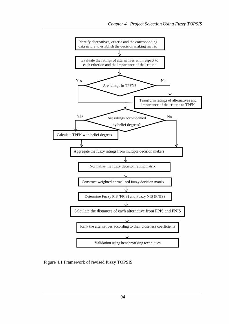
Chapter 4. Project Selection Using Fuzzy TOPSIS
94
Figure 4.1 Framework of revised fuzzy TOPSIS
Determine Fuzzy PIS (FPIS) and Fuzzy NIS (FNIS)
Construct weighted normalized fuzzy decision matrix
Identify alternatives, criteria and the corresponding
data nature to establish the decision making matrix
format
Evaluate the ratings of alternatives with respect to
each criterion and the importance of the criteria
cision making matrix format
Are ratings in TPFN?
Transform ratings of alternatives and
importance of the criteria to TPFN
cision making matrix
Aggregate the fuzzy ratings from multiple decision makers
Normalise the fuzzy decision rating matrix
Calculate the distances of each alternative from FPIS and FNIS
Rank the alternatives according to their closeness coefficients
Validation using benchmarking techniques
No Yes
Are ratings accompanied
by belief degrees?
Yes No
Calculate TPFN with belief degrees
matrix format

Chapter 4. Project Selection Using Fuzzy TOPSIS
95
4.4.1 Identify Alternatives and Criteria to Establish the Decision Making
Matrix Format with the Presentation of All Alternatives and Criteria
In order to capture raw data, the matrix D can be established to include various data
types and it can be expressed as below:
𝐶 ⋯ 𝐶𝑗 ⋯ 𝐶𝑛
𝐷
𝐴
⋮𝐴𝑖
⋮𝐴𝑚 [
𝑥
⋮
𝑥 ⋯
⋮𝑥 𝑛
⋮𝑥𝑖 ⋯
⋮
𝑥𝑖𝑗 ⋯
⋮
𝑥𝑖𝑛
⋮𝑥𝑚 ⋯ 𝑥𝑚𝑗 ⋯ 𝑥𝑚𝑛]
(4.1)
𝑊 [�̃�1 �̃�𝑗 �̃�𝑛],
where each 𝐴𝑖 represent alternative i considered; 𝐶𝑗 is the criterion used to measure
the performance of each alternative; and 𝑥𝑖𝑗 is the rating of the ith alternative with
respect to the jth criterion and can be described by a TPFN, 𝑥𝑖𝑗 𝑎𝑖𝑗 𝑏𝑖𝑗 𝑐𝑖𝑗 𝑑𝑖𝑗 , a
triangular fuzzy number 𝑥𝑖𝑗 (𝑎𝑖𝑗 𝑏𝑖𝑗 𝑑𝑖𝑗) a crisp number 𝑥𝑖𝑗 𝑎𝑖𝑗 , a range
number 𝑥𝑖𝑗 𝑎𝑖𝑗 𝑑𝑖𝑗 or a pre-defined linguistic variable with belief degree. The
TPFNs of the linguistic variables are pre-defined and presented in Table 4.1. �̃�𝑗 is
the subjective importance estimation of the jth criterion and can be assessed using
linguistic variables, which are described by TPFNs in Table 4.2.
4.4.2 Evaluate the Ratings of Alternatives with Respect to Each Criterion and
the Importance of the Criteria, �̃�𝒋
It is often difficult for experts to give a confident assessment of the alternatives by
only using single linguistic terms. They might not be able to establish a strong
correlation between the evaluations and the pre-defined linguistic variables. There
are assessors who prefer to give a range of numerical values or a precise numerical
value especially when objective information is known to support their evaluations.
Therefore, in order to collect raw data as comprehensively as possible, four options
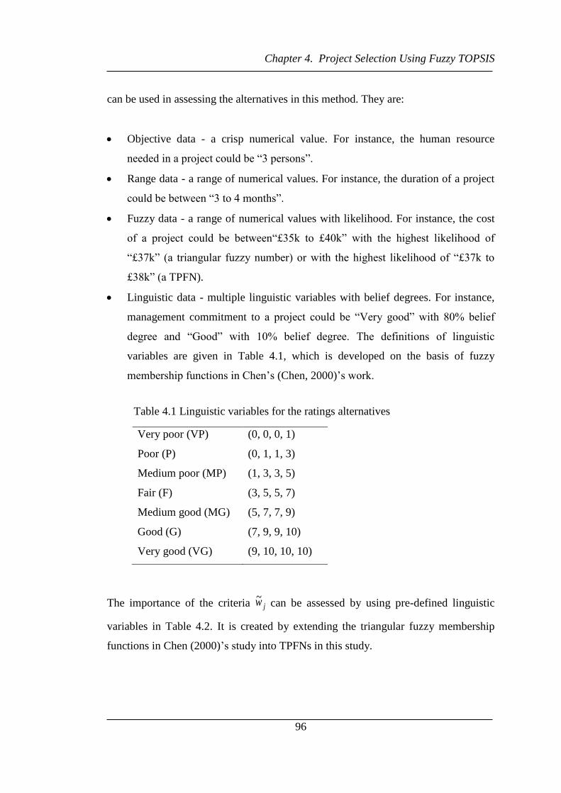
Chapter 4. Project Selection Using Fuzzy TOPSIS
96
can be used in assessing the alternatives in this method. They are:
Objective data - a crisp numerical value. For instance, the human resource
needed in a project could be “3 persons”.
Range data - a range of numerical values. For instance, the duration of a project
could be between “3 to 4 months”.
Fuzzy data - a range of numerical values with likelihood. For instance, the cost
of a project could be between“£35k to £40k” with the highest likelihood of
“£37k” (a triangular fuzzy number) or with the highest likelihood of “£37k to
£38k” (a TPFN).
Linguistic data - multiple linguistic variables with belief degrees. For instance,
management commitment to a project could be “Very good” with 80% belief
degree and “Good” with 10% belief degree. The definitions of linguistic
variables are given in Table 4.1, which is developed on the basis of fuzzy
membership functions in Chen’s (Chen, 2000)’s work.
Table 4.1 Linguistic variables for the ratings alternatives
Very poor (VP) (0, 0, 0, 1)
Poor (P) (0, 1, 1, 3)
Medium poor (MP) (1, 3, 3, 5)
Fair (F) (3, 5, 5, 7)
Medium good (MG) (5, 7, 7, 9)
Good (G) (7, 9, 9, 10)
Very good (VG) (9, 10, 10, 10)
The importance of the criteria jw~ can be assessed by using pre-defined linguistic
variables in Table 4.2. It is created by extending the triangular fuzzy membership
functions in Chen (2000)’s study into TPFNs in this study.

Chapter 4. Project Selection Using Fuzzy TOPSIS
97
Table 4.2 Linguistic variables for the importance weight of each criterion
Very low (VL) (0, 0, 0, 0.1)
Low (L) (0, 0.1, 0.1 0.3)
Medium low (ML) (0.1, 0.3, 0.3, 0.5)
Medium (M) (0.3, 0.5, 0.5, 0.7)
Medium high (MH) (0.5, 0.7, 0.7, 0.9)
High (H) (0.7, 0.9, 0.9, 1)
Very high (VH) (0.9, 1, 1, 1)
4.4.3 Transform Ratings of Alternatives to TPFN
Traditional fuzzy TOPSIS is not capable of handling different types of data
simultaneously. In this new fuzzy TOPSIS method, a data transformation mechanism
is developed based on TPFNs to unify the various data formats into a TPFN form as
follows.
Objective data,𝑥𝑖𝑗 𝑎𝑖𝑗 can be transformed to �̃�𝑖𝑗 𝑎𝑖𝑗 𝑏𝑖𝑗 𝑐𝑖𝑗 𝑑𝑖𝑗 , where
𝑎𝑖𝑗 𝑏𝑖𝑗 𝑐𝑖𝑗 𝑑𝑖𝑗.
Range data, 𝑥𝑖𝑗 𝑎𝑖𝑗 𝑏𝑖𝑗 can be transformed to �̃�𝑖𝑗 𝑎𝑖𝑗 𝑏𝑖𝑗 𝑐𝑖𝑗 𝑑𝑖𝑗 , where
𝑎𝑖𝑗 𝑏𝑖𝑗 𝑐𝑖𝑗 𝑑𝑖𝑗.
Fuzzy data, a triangular fuzzy number 𝑥𝑖𝑗 (𝑎𝑖𝑗 𝑏𝑖𝑗 𝑑𝑖𝑗) can be transformed to
�̃�𝑖𝑗 𝑎𝑖𝑗 𝑏𝑖𝑗 𝑐𝑖𝑗 𝑑𝑖𝑗 , where 𝑏𝑖𝑗 𝑐𝑖𝑗 . There is no need to transform any
TPFN data.
Linguistic data, if the input data is presented by a single linguistic term with
100% belief degree, then it can be presented by the TPFN of the term in Table
4.1. If the input data is described by multiple linguistic terms with partial belief
degrees to each, then its TPFN can be calculated as follows.
If the belief degree is complete ( ∑ 𝛽𝑖𝑗ℎ7
ℎ= 1 ), then the TPFN of the input

Chapter 4. Project Selection Using Fuzzy TOPSIS
98
evaluation is:
�̃�𝑖𝑗 ∑ 𝛽𝑖𝑗ℎ7
ℎ= 𝑓ℎ (4.2)
where 𝛽𝑖𝑗ℎ stands for the degree of belief for the ℎ𝑡ℎ linguistic variable in Table 4.1
used to describe the fuzzy rating of the ith alternative with respect to the jth criterion;
and 𝑓ℎ represents the TPFN of the ℎ𝑡ℎ linguistic variable.
If the belief degree is incomplete (∑ 𝛽𝑖𝑗ℎ7
ℎ= < 1 , the remaining degrees of belief
(1 − ∑ 𝛽𝑖𝑗ℎ7
ℎ= need to be re-assigned to both grades of the first/lowest and the
last/highest ratings. Let �̃�𝑖𝑗𝐿 𝑎𝑛𝑑 �̃�𝑖𝑗
𝐻 stand for the evaluations when the remaining
degree of belief is re-assigned to the first/lowest rating and last/highest rating,
respectively. When assigning the remainder to the lowest grade, the TPFN for the
evaluation �̃�𝑖𝑗𝐿 can be calculated as:
�̃�𝑖𝑗𝐿 (𝑎𝑖𝑗
𝐿 𝑏𝑖𝑗𝐿 𝑐𝑖𝑗
𝐿 𝑑𝑖𝑗𝐿 ) ∑ 𝛽𝑖𝑗
ℎ7ℎ= 𝑓ℎ + 1 − ∑ 𝛽𝑖𝑗
ℎ7ℎ= 𝑓 (4.3)
When assigning the remaining to the highest rating, the TPFN for the evaluation �̃�𝑖𝑗𝐻
can be calculated as:
�̃�𝑖𝑗𝐻 (𝑎𝑖𝑗
𝐻 𝑏𝑖𝑗𝐻 𝑐𝑖𝑗
𝐻 𝑑𝑖𝑗𝐻) ∑𝛽𝑖𝑗
ℎ
7
ℎ=
𝑓ℎ + 1 − ∑𝛽𝑖𝑗ℎ
7
ℎ=
𝑓7 (4.4)
The two TPFNs can be combined into one set of TPFN to cover the membership
ranges of the highest and lowest ratings using:
�̃�𝑖𝑗 (𝑎𝑖𝑗 𝑏𝑖𝑗 𝑐𝑖𝑗 𝑑𝑖𝑗)
[min(𝑎𝑖𝑗𝐿 𝑎𝑖𝑗
𝐻) min(𝑏𝑖𝑗𝐿 𝑏𝑖𝑗
𝐻) max(𝑐𝑖𝑗𝐿 𝑐𝑖𝑗
𝐻) max(𝑑𝑖𝑗𝐿 𝑑𝑖𝑗
𝐻)]
(4.5)
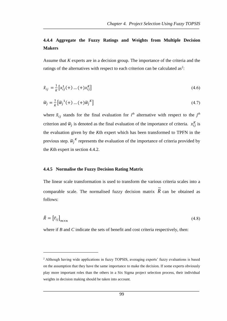
Chapter 4. Project Selection Using Fuzzy TOPSIS
99
4.4.4 Aggregate the Fuzzy Ratings and Weights from Multiple Decision
Makers
Assume that K experts are in a decision group. The importance of the criteria and the
ratings of the alternatives with respect to each criterion can be calculated as2:
�̃�𝑖𝑗
𝐾[𝑥𝑖𝑗
+ + 𝑥𝑖𝑗𝐾] (4.6)
�̃�𝑗
𝐾[�̃�𝑗
+ + �̃�𝑗𝐾] (4.7)
where �̃�𝑖𝑗 stands for the final evaluation for ith alternative with respect to the jth
criterion and �̃�𝑗 is denoted as the final evaluation of the importance of criteria. 𝑥𝑖𝑗𝐾 is
the evaluation given by the Kth expert which has been transformed to TPFN in the
previous step. �̃�𝑗𝐾
represents the evaluation of the importance of criteria provided by
the Kth expert in section 4.4.2.
4.4.5 Normalise the Fuzzy Decision Rating Matrix
The linear scale transformation is used to transform the various criteria scales into a
comparable scale. The normalised fuzzy decision matrix R~
can be obtained as
follows:
�̃� [�̃�𝑖𝑗]𝑚×𝑛 (4.8)
where if B and C indicate the sets of benefit and cost criteria respectively, then:
2 Although having wide applications in fuzzy TOPSIS, averaging experts’ fuzzy evaluations is based
on the assumption that they have the same importance to make the decision. If some experts obviously
play more important roles than the others in a Six Sigma project selection process, their individual
weights in decision making should be taken into account.

Chapter 4. Project Selection Using Fuzzy TOPSIS
100
�̃�𝑖𝑗 (𝑎𝑖𝑗
𝑑𝑗∗
𝑏𝑖𝑗
𝑑𝑗∗
𝑐𝑖𝑗
𝑑𝑗∗
𝑑𝑖𝑗
𝑑𝑗∗) 𝑗 ∈ 𝐵
�̃�𝑖𝑗 (𝑎𝑗
−
𝑑𝑖𝑗 𝑎𝑗
−
𝑐𝑖𝑗 𝑎𝑗
−
𝑏𝑖𝑗 𝑎𝑗
−
𝑎𝑖𝑗) 𝑗 ∈ 𝐶
𝑑𝑗∗ max𝑑𝑖𝑗 𝑖𝑓 𝑗 ∈ 𝐵
𝑎𝑗− min𝑎𝑖𝑗 𝑖𝑓 𝑗 ∈ 𝐶
4.4.6 Constructed Weighted Normalized Fuzzy Decision Matrix
The weighted normalized fuzzy decision matrix can be constructed by multiplying
the normalized fuzzy decision matrix R~
with the aggregated weights jw~ as follows:
nmijvV ]~[~
i= 1, 2, …,m, j= 1, 2, …, n (4.9)
where jijij wrv ~)(~~ . �̃� is the weighted normalized fuzzy decision matrix. ijv~ are
normalized positive trapezoidal fuzzy numbers with the value ranges belonging to
the close interval [0, 1].
4.4.7 Determine FPIS and FNIS
From the weighted normalised fuzzy decision matrix V~
, it can be clearly seen that
each element ijv~ represents a normalised TPFN with a value range belonging to the
close interval [0, 1]. Therefore, FPIS *A and FNIS A can be separately defined as:
)~,,~,,~( ***1
*nj vvvA
)~,,~,,~( 1 nj vvvA (4.10)
where �̃�𝑗∗ 1 1 1 1 and �̃�𝑗
− 0 0 0 0 , j = 1, 2, …, n.

Chapter 4. Project Selection Using Fuzzy TOPSIS
101
4.4.8 Calculate the Distances of Each Alternative from FPIS and FNIS
The distances of each alternative from *A and
A can be calculated using
Euclidean distance measurement between two fuzzy numbers as follows:
𝑑𝑖∗ ∑ 𝑑(�̃�𝑖𝑗 �̃�𝑗
∗)𝑛𝑗= ∑ √
4[( v
ija − 1)
+ ( v
ijb − 1)
+ ( v
ijc − 1)
+ ( v
ijd − 1)
]𝑛𝑗=
𝑖 1 2 𝑚 (4.11)
𝑑𝑖− ∑ 𝑑(�̃�𝑖𝑗 �̃�𝑗
−)𝑛𝑗= ∑ √
4[( v
ija − 0)
+ ( v
ijb − 0)
+ ( v
ijc − 0)
+ ( v
ijd − 0)
]𝑛𝑗=
𝑖 1 2 𝑚 (4.12)
where i = 1, 2, …, m; ),,,(~ v
ij
v
ij
v
ij
v
ijij dcbav .
4.4.9 Calculate the Distance Closeness Coefficient of Each Alternative
The distance closeness coefficient of each alternative can be obtained by using
Equation (4.13)
ii
ii
dd
dCC
*
i= 1, 2, …,m (4.13)
4.4.10 Rank the Alternatives According to their Closeness Coefficients
Obviously, an alternative iA is closer to the FPIS *A and further from the FNIS
A
as iCC approaches 1. Therefore, the larger the value iCC , the more preferred the
alternative it represents. The best alternative can be identified as the one with the
largest iCC value.
Chapter 4. Project Selection Using Fuzzy TOPSIS
102
4.4.11 Validation using Benchmarking Techniques
In this study, a benchmarking technique is used to compare the new fuzzy TOPSIS
method with the approximate TOPSIS by Yang et al. (2011) A case analysis is first
carried out to demonstrate the feasibility of the new method through the Six Sigma
project selection of a world leading shipping company. Second, Yang et al.’s method
is used with the same input data to test the soundness of the new method. While the
new method is validated by obtaining similar outputs as those from an established
model, it also shows the superiority over the established one in simplifying
calculation and improving the accuracy of results.
4.5 Six Sigma Project Selections Using the Revised TOPSIS
An illustrative example is given in this section to demonstrate the use of the new
fuzzy TOPSIS in Six Sigma project selection. A world leading shipping company
started a Six Sigma programme in order to reduce costs and increase customer
satisfaction. At an initial stage, four Six Sigma projects were identified. However,
due to the limitation of resources, the management team would like to select one to
start with which will maximally benefit the company within a short period.
4.5.1 Identify Alternatives, Criteria and the Corresponding Data Nature to
Establish the Decision Making Matrix Format
The case was to select the best project to suit the current needs of the company for
cost savings in a short term. Four identified projects (alternatives) were 𝐴 : Reduce
the number of incorrect invoices, 𝐴 : Reduce the number of wasted journeys, 𝐴3:
Reduce unbilled charges and 𝐴4: Reduce lead-time in query resolving.
The selection of Six Sigma needs to align with the strategic objectives and priorities
of an organization. It is a very important decision to make for organizations as Six

Chapter 4. Project Selection Using Fuzzy TOPSIS
103
Sigma projects require different resources (capital, time and labour etc.). Studies
show that during the project selection process, companies overemphasise financial
savings and the applicability of Six Sigma (Nonthaleerak and Hendry, 2008).
Researchers have proposed different criteria in Six Sigma project selection in the
form of generic criteria. Table 4.3 displays some typical criteria from previous
studies.
Table 4.3 Six Sigma project selection criteria overview
Author Proposed criteria
Pande et al. (2000) Business benefits criteria
Feasibility criteria
Organization impact criteria
Harry and Schroeder (2006)
Defects per million opportunities
Net cost savings
COPQ
Cycle time
Customer satisfaction
Capacity
Internal performance
Banuelas et al. (2006)
Customer impact
Financial impact
Top management commitment
Measurable and feasible
Learning and growth
Connected to business strategy and core
competence
Bilgen and Sen (2012)
Resources (Cost, Time, Labour)
Benefits (Saving, Productivity, Scrap
yield decrease)
Effects (Quality, Capacity, Energy)
Pande et al. (2000) indicated that there should not be too many factors in project
selection. Though different projects may have different targets to achieve depending
on industrial requirements and company needs, there is no doubt that every project
requires multiple resources (e.g. capital and labour, etc.) and aims to achieve certain

Chapter 4. Project Selection Using Fuzzy TOPSIS
104
benefits (e.g. cost saving) at a manageable risk level. Therefore, in this case, three
main criteria – Cost, Benefit and Risk, with sub-criteria (shown in Figure 4.2) are
identified by a team of senior managers of the shipping company using a
brainstorming technique. The identified criteria and sub-criteria could vary subject to
the development strategies of different companies. From Figure 4.2, the project
selection criteria are denoted by 𝐶 : Financial expenses, 𝐶 : Project duration, 𝐶3 :
Human resources, 𝐶4: Cost savings, 𝐶5: Increase productivity, 𝐶6: Increase customer
satisfaction, 𝐶7: Applicability of the project, 𝐶8: Connect to business strategy, 𝐶9:
Top management commitment.
Figure 4.2 Project selection criteria with sub-criteria
4.5.2 Evaluate the Ratings of Alternatives with Respect to Each Criterion and
the Importance of the Criteria, �̃�𝒋
The selected criteria need to be prioritised as the ones most critical to the overall
success of the organisation will have the most impact on the project selection. Three
decision makers (𝐷𝑀 𝐷𝑀 𝑎𝑛𝑑 𝐷𝑀3 including the chief operation officer, the
chief finance officer and a Six Sigma MBB participated in the project selection
process. They used Table 4.2 to provide their evaluations of the importance of the
criteria and Table 4.1 for rating each alternative against every criterion. The
evaluations are presented in Table 4.4 and Table 4.5 respectively, in which some
Project selection
criteria
Cost
Benefit
Risk
Financial expenses
Duration
Human Resources
Cost savings
Increase productivity
Increase customer satisfaction
Applicability of the project
Connect to business strategy
Top management commitment

Chapter 4. Project Selection Using Fuzzy TOPSIS
105
descriptions (e.g. 90% MG evaluation of A1 with respect to C9 from DM1) reveal the
incomplete knowledge of the decision makers.
Table 4.4 The importance weight of the criteria given by decision makers
𝐶 𝐶 𝐶3 𝐶4 𝐶5 𝐶6 𝐶7 𝐶8 𝐶9
DM1 H VH H VH MH H H MH H
DM2 MH VH H VH MH H VH MH VH
DM3 H VH H VH MH MH VH H H
VL – Very low, L – Low, ML – Medium low, M – Medium, MH – Medium high, H – High, VH – Very high
Table 4.5 The rating of alternatives by decision makers under all criteria
c 𝐶 𝐶 𝐶3 𝐶4 𝐶5 𝐶6 𝐶7 𝐶8 𝐶9
𝐴
DM1 G 5M 3 G G VG G G 90%MG
DM2 G 5-6M 5 MG G VG 90%G G F
DM3 G 5-6M 4-5 MG G G MG G F
𝐴
DM1 F 6M 5-6 G F MG G G 90%G
DM2 F 6-7M 6-8 VG MG G G G G
DM3 F 6M 6 G F G G G G
𝐴3
DM1 G 3M 3 F MP 80%F,20%MP VG VG VG
DM2 G 2-3M 3 MG F F VG G G
DM3 G 3M 3 F F F VG G G
𝐴4
DM1 G 4M 4 MP MG VG G VG 90%MG
DM2 G 5-6M 4-5 MP G G MG G MG
DM3 G 5M 4-5 P MG VG G G G
VP – Very poor, P – Poor, MP – Medium poor, F – Fair, MG – Medium good, G – Good, VG – Very good
M under C2 stands for” Month”
4.5.3 Transform Ratings of Alternatives to TPFN and Aggregate the Fuzzy
Ratings from Multiple Decision Makers
Once the assessments from decision makers are obtained, they can all be transformed
to TPFNs to establish a fuzzy decision matrix. Based on information in Table 4.5,

Chapter 4. Project Selection Using Fuzzy TOPSIS
106
different types of data can be converted into a common form using the fuzzy
transformation mechanism in Section 4.4.3.
Objective data. For instance, the evaluation from 𝐷𝑀 for alternative A
regarding criterion C is 5M. It can be transformed to a TPFN of (5, 5, 5, 5).
Range data. For instance, the evaluation from DM2 for alternative A regarding
criterion C is 5-6M. It can be transformed to a TPFN of (5, 5, 6, 6).
Linguistic data. For instance, the evaluation from DM1 for alternative A3
regarding criterion C6 was provided with a complete belief degree and the TPFN
can be calculated by using Equation (4.2).
�̃�3 6 ∑ 𝛽3 6ℎℎ𝑗
ℎ= 𝑓ℎ 0.8 × 3 5 5 7 + 0.2 × 1 3 3 5 2.6 4.6 4.6 6.6
The evaluations from 𝐷𝑀 for alternatives A A and A4 with regards to criterion C9
and from 𝐷𝑀 for alternative A with regards to criterion C7 were provided with
incomplete belief degrees and the TPFNs can be calculated by using Equations (4.3),
(4.4) and (4.5). Taking 𝐷𝑀 , for alternative A against C9 as an example where the
evaluation is 90% MG.
�̃� 9𝐿 (𝑎 9
𝐿 𝑏 9𝐿 𝑐 9
𝐿 𝑑 9𝐿 ) ∑ 𝛽 9
ℎ7ℎ= 𝑓ℎ + 1 − ∑ 𝛽 9
ℎ7ℎ= 𝑓
0.9 × 5 7 7 9 + 0.1 × 0 0 0 1 4.6 6.3 6.3 8.2
�̃�𝑖𝑗𝐻 (𝑎𝑖𝑗
𝐻 𝑏𝑖𝑗𝐻 𝑐𝑖𝑗
𝐻 𝑑𝑖𝑗𝐻) ∑ 𝛽𝑖𝑗
ℎ7ℎ= 𝑓ℎ + 1 − ∑ 𝛽𝑖𝑗
ℎℎ𝑗
ℎ= 𝑓7
0.9 × 5 7 7 9 + 0.1 × 9 10 10 10 5.4 7.3 7.3 9.1
�̃�𝑖𝑗 (𝑎𝑖𝑗 𝑏𝑖𝑗 𝑐𝑖𝑗 𝑑𝑖𝑗)
[min(𝑎𝑖𝑗𝐿 𝑎𝑖𝑗
𝐻) min(𝑏𝑖𝑗𝐿 𝑏𝑖𝑗
𝐻) max(𝑐𝑖𝑗𝐿 𝑐𝑖𝑗
𝐻) max(𝑑𝑖𝑗𝐿 𝑑𝑖𝑗
𝐻)]
4.6 6.3 7.3 9.1
In a similar way, all the other input data in Table 4.5 can be transformed in TPFNs.
All the TPFNs are then aggregated by using Equations (4.6) and (4.7). The results are

Chapter 4. Project Selection Using Fuzzy TOPSIS
107
shown in Table 4.6 and Table 4.7
4.5.4 Normalise the Fuzzy Decision Rating Matrix
The transformed ratings are normalized by using Equation (4.8). Taking alternative
A with regards to criterion 𝐶 as an example, 𝐶 is a cost criterion and 𝑎 −
min𝑎𝑖 = 2.67. Consequently, the normalized rating can be calculated as:
�̃� (𝑎
−
𝑑 𝑎
−
𝑐 𝑎
−
𝑏 𝑎
−
𝑎 ) (
2.67
5.67 2.67
5.67 2.67
5 2.67
5) 0.47 0.47 0.53 0.53
The same can be calculated for all the other ratings. The results of the normalised
matrix are shown in Table 4.8.
4.5.5 Constructed Weighted Normalized Fuzzy Decision Matrix
The weights of criteria are built in the matrix by using Equation (4.9) and the results
are listed in Table 4.9. For example, the weighted normalised fuzzy evaluation of
alternative 𝐴 with regards to criterion 𝐶 can be computed as
11,11,1~)(~~ wrv i = (0.7,0.9,0.9,1) × (0.63,0.83,0.83,0.97) = (0.44,0.75,0.75,0.97)
4.5.1 Determine FPIS and FNIS
From Equation (4.10), the following are obtained.
𝐴∗ [ 1 1 1 1 1 1 1 1 1 1 1 1 1 1 1 1 1 1 1 1 1 1 1 1 1 1 1 1 1 1 1 1 1 1 1 1 ]
𝐴− [ 0 0 0 0 0 0 0 0 0 0 0 0 0 0 0 0 0 0 0 0 0 0 0 0 0 0 0 0 0 0 0 0 0 0 0 0 ]

Chapter 4. Project Selection Using Fuzzy TOPSIS
108
Table 4.6 The importance weight of the criteria in TPFN
𝐶 𝐶 𝐶3 𝐶4 𝐶5 𝐶6 𝐶7 𝐶8 𝐶9
DM1 (0.7,0.9,0.9,1.0) (0.9,1.0,1.0,1.0) (0.7,0.9,0.9,1.0) (0.9,1.0,1.0,1.0) (0.5,0.7,0.7,0.9) (0.7,0.9,0.9,1.0) (0.7,0.9,0.9,1.0) (0.5,0.7,0.7,0.9) (0.7,0.9,0.9,1.0)
DM2 (0.5,0.7,0.7,0.9) (0.9,1.0,1.0,1.0) (0.7,0.9,0.9,1.0) (0.9,1.0,1.0,1.0) (0.5,0.7,0.7,0.9) (0.7,0.9,0.9,1.0) (0.9,1.0,1.0,1.0) (0.5,0.7,0.7,0.9) (0.9,1.0,1.0,1.0)
DM3 (0.7,0.9,0.9,1.0) (0.9,1.0,1.0,1.0) (0.7,0.9,0.9,1.0) (0.9,1.0,1.0,1.0) (0.5,0.7,0.7,0.9) (0.5,0.7,0.7,0.9) (0.9,1.0,1.0,1.0) (0.7,0.9,0.9,1.0) (0.7,0.9,0.9,1.0)
�̃� (0.63,0.83,0.83,0.97) (0.9,1.0,1.0,1.0) (0.7,0.9,0.9,1.0) (0.9,1.0,1.0,1.0) (0.5,0.7,0.7,0.9) (0.63,0.83,0.83,0.97) (0.83,0.97,0.97,1) (0.57,0.77,0.77,0.93) (0.7,0.9,0.9,1.0)
Table 4.7 The rating of alternatives by decision makers under all criteria in TPFN
c 𝐶 𝐶 𝐶3 𝐶4 𝐶5 𝐶6 𝐶7 𝐶8 𝐶9
𝐴
DM1 (7,9,9,10) (5,5,5,5) (3,3,3,3) (7,9,9,10) (7,9,9,10) (9,10,10,10) (7,9,9,10) (7,9,9,10) (4.6,6.3,7.3,9.1)
DM2 (7,9,9,10) (5,5,6,6) (5,5,5,5) (5,7,7,9) (7,9,9,10) (9,10,10,10) (6.3,8.1,9.1,10) (7,9,9,10) (3,5,5,7)
DM3 (7,9,9,10) (5,5,6,6) (4,4,5,5) (5,7,7,9) (7,9,9,10) (7,9,9,10) (5,7,7,9) (7,9,9,10) (3,5,5,7)
𝐴 𝑗 (7,9,9,10) (5,5,5.67,5.67) (4,4,4.33,4.33) (5.67,7.67,7.67, 9.33) (7,9,9,10) (8.33,9.67,9.67,10) (5.67,7.67,7.67,9.33) (7,9,9,10) (3.67,5.67,5.67,7.67)
𝐴
DM1 (3,5,5,7) (6,6,6,6) (5,5,5,5) (7,9,9,10) (3,5,5,7) (5,7,7,9) (7,9,9,10) (7,9,9,10) (6.3,8.1,9.1,10)
DM2 (3,5,5,7) (6,6,7,7) (6,6,8,8) (9,10,10,10) (5,7,7,9) (5,7,7,9) (7,9,9,10) (7,9,9,10) (7,9,9,10)
DM3 (3,5,5,7) (6,6,6,6) (6,6,6,6) (9,9,10,10) (3,5,5,7) (7,9,9,10) (7,9,9,10) (7,9,9,10) (7,9,9,10)
𝐴 𝑗 (3,5,5,7) (6,6,6.33,6.33) (5.67,5.67,6.33,6.33) (8.33,9.67,9.67,10) (3.67,5.67,5.67,7.67) (5.67,7.67,7.67, 9.33) (7,9,9,10) (7,9,9,10) (7,9,9,10)
𝐴3
DM1 (7,9,9,10) (3,3,3,3) (3,3,3,3) (3,5,5,7) (1,3,3,1) (2.6,4.6,4.6,6.6) (9,10,10,10) (9,10,10,10) (9,10,10,10)
DM2 (7,9,9,10) (2,2,3,3) (3,3,3,3) (5,7,7,9) (3,5,5,7) (3,5,5,7) (9,10,10,10) (7,9,9,10) (7,9,9,10)
DM3 (7,9,9,10) (3,3,3,3) (3,3,3,3) (3,5,5,7) (3,5,5,7) (3,5,5,7) (9,10,10,10) (7,9,9,10) (7,9,9,10)
𝐴3𝑗 (7,9,9,10) (2.67,2.67,3,3) (3,3,3,3) (3.67,5.67,5.67,7.67) (2.33,4.33,4.33,6.33) (3,5,5,7) (9,10,10,10) (7.63,9.33,9.33,10) (7.63,9.33,9.33,10)

Chapter 4. Project Selection Using Fuzzy TOPSIS
109
𝐴4
DM1 (7,9,9,10) (4,4,4,4) (4,4,4,4) (1,3,3,5) (5,7,7,9) (9,10,10,10) (7,9,9,10) (9,10,10,10) (4.6,6.3,7.3,9.1)
DM2 (7,9,9,10) (5,5,6,6) (4,4,5,5) (1,3,3,5) (7,9,9,10) (7,9,9,10) (5,7,7,9) (7,9,9,10) (5,7,7,9)
DM3 (7,9,9,10) (5,5,5,5) (4,4,5,5) (0,1,1,3) (5,7,7,9) (9,10,10,10) (7,9,9,10) (7,9,9,10) (7,9,9,10)
𝐴4𝑗 (7,9,9,10) (4.67,4.67,5,5) (4,4,4.67,4.67) (0.67,2.33,2.33,4.33)
(5.67,7.67,7.67,
9.33) (8.33,9.67,9.67,10) (6.33,8.33,8.33,9.67) (7.67,9.33,9.33,10) (5.67,7.67,7.67, 9.33)
Table 4.8 Normalized fuzzy decision matrix
𝐶 𝐶 𝐶3 𝐶4 𝐶5 𝐶6 𝐶7 𝐶8 𝐶9
𝐴 (0.7,0.9,0.9,1) (0.47,0.47,0.53,0.53) (0.69,0.69,0.75,0.75) (0.57,0.77,0.77,0.93) (0.7,0.9,0.9,1) (0.83,0.97,0.97,1) (0.61,0.8,0.84,0.97) (0.7,0.9,0.9,1) (0.35,0.54,0.58,0.77)
𝐴 (0.3,0.5,0.5,0.7) (0.42,0.42,0.44,0.44) (0.47,0.47,0.53,0.53) (0.83,0.97,0.97,1) (0.37,0.57,0.57,0.77) (0.57,0.77,0.77,0.93) (0.7,0.9,0.9,1) (0.7,0.9,0.9,1) (0.68,0.87,0.9,1)
𝐴3 (0.7,0.9,0.9,1) (0.89,0.89,1,1) (1,1,1,1) (0.37,0.57,0.57,0.77) (0.23,0.43,0.43,0.63) (0.29,0.49,0.49,0.69) (0.9,1,1,1) (0.77,0.93,0.93,1) (0.77,0.93,0.93,1)
𝐴4 (0.7,0.9,0.9,1) (0.53,0.53,0.57,0.57) (0.64,0.64,0.75,0.75) (0.07,0.23,0.23,0.43) (0.57,0.77,0.77,0.93) (0.83,0.97,0.97,1) (0.63,0.83,0.83,0.97) (0.77,0.93,0.93,1) (0.55,0.74,0.78,0.94)
Table 4.9 Weighted normalized fuzzy decision matrix
𝐶 𝐶 𝐶3 𝐶4 𝐶5 𝐶6 𝐶7 𝐶8 𝐶9
𝐴 (0.44,0.75,0.75,0.97) (0.42,0.47,0.53,0.53) (0.48,0.62,0.68,0.75) (0.51,0.77,0.77,0.93) (0.35,0.63,0.63,0.9) (0.53,0.81,0.81,0.97) (0.51,0.78,0.81,0.97) (0.4,0.69,0.69,0.93) (0.27,0.51,0.54,0.77)
𝐴 (0.19,0.42,0.42,0.68) (0.38,0.42,0.44,0.44) (0.33,0.43,0.48,0.53) (0.75,0.97,0.97,1) (0.18,0.4,0.4,0.69) (0.36,0.64,0.64,0.9) (0.58,0.87,0.87,1) (0.4,0.69,0.69,0.93) (0.52,0.81,0.84,1)
𝐴3 (0.44,0.75,0.75,0.97) (0.8,0.89,1,1) (0.7,0.9,0.9,1) (0.33,0.57,0.57,0.77) (0.12,0.3,0.3,0.57) (0.18,0.41,0.41,0.66) (0.75,0.97,0.97,1) (0.43,0.72,0.72,0.93) (0.59,0.87,0.87,1)
𝐴4 (0.44,0.75,0.75,0.97) (0.48,0.53,0.57,0.57) (0.45,0.58,0.68,0.75) (0.06,0.23,0.23,0.43) (0.28,0.54,0.54,0.84) (0.53,0.81,0.81,0.97) (0.53,0.81,0.81,0.97) (0.43,0.72,0.72,0.93) (0.42,0.69,0.72,0.94)

Chapter 4. Project Selection Using Fuzzy TOPSIS
110
4.5.2 Calculate the Distances of Each Alternative from FPIS and FNIS
The distances from alternatives to FPIS and FNIS are calculated using Equations
(4.11) and (4.12). For example, the distances from A to FPIS and FNIS with respect
to C4 can be computed as:
𝑑 4∗ 𝑑(�̃� 4 �̃�4
∗) √
4[ 0.51 − 1 + 0.77 − 1 + 0.77 − 1 + 0.93 − 1 ]
0.3
𝑑 4− 𝑑(�̃� 4 �̃�4
−) √
4[ 0.51 − 0 + 0.77 − 0 + 0.77 − 0 + 0.93 − 0 ]
0.76
Similarly, the individual distances from A to FPIS and FNIS with respect to the other
criteria can be obtained, respectively. The total distances from A to FPIS and FNIS
can then be computed by adding all the obtained individual distances together.
Consequently, the distances from all alternatives to FPIS and FNIS with regard to all
the criteria are obtained and shown in Table 4.10.
Table 4.10 Distances of each alternative from FPIS and FNIS
𝐴∗ 𝐴−
𝐴 3.41 6.09
𝐴 3.75 5.74
𝐴3 3.08 6.45
𝐴4 3.7 5.8
4.5.3 Calculate the Distance Closeness Coefficient of Each Alternative
By using Equation (4.13) in section 4.4.9, the distance closeness coefficient can be
calculated as:

Chapter 4. Project Selection Using Fuzzy TOPSIS
111
64.01
*
1
11
dd
dCC
Similarly, 𝐶𝐶 0.6 𝐶𝐶3 0.68 and 𝐶𝐶4 0.61 can be obtained. According to
the closeness coefficient, the ranking order of the four alternatives is 𝐴3> 𝐴 > 𝐴4 >
𝐴 . It means that based on the current needs of the organization, the best Six Sigma
project to be selected is “Reduce unbilled charges”, while the last choice is “Reduce
lead time in query resolving”.
4.5.4 Validation using Benchmarking Techniques
In order to validate the soundness and reliability of the new fuzzy TOPSS approach,
the original input in terms of alternative rating and the importance of criteria in Table
4.4 and Table 4.5 are used in Yang et al. (2011)’s approximate TOPSIS. If the new
fuzzy TOPSIS is reliable, the output from the approximate TOPSIS should be kept in
harmony with the above result to a significant extent. Furthermore, to demonstrate
the superiority of the new method, the main calculation processes of the approximate
TOPSIS by Yang et al. are provided as follows.
The PBR and PWR matrices are presented in Table 4.11 and Table 4.12. The results
of the normalized matrix are shown in Table 4.13 and Table 4.14. Because of the
possible best and worst rating matrices, the calculation demands twice the effort and
time compared with the new fuzzy TOPSIS method in this study.
The results from the approximate TOPSIS are obtained and presented in intervals as:
𝐶𝐶 0.57 0.59 with average value 0.58
𝐶𝐶 0.47 0.48 with average value 0.475
𝐶𝐶3 0.69 0.7 with average value 0.695
𝐶𝐶4 0.56 0.57 with average value 0.565
Chapter 4. Project Selection Using Fuzzy TOPSIS
112
It is not possible to compare the range data to draw a definite conclusion (unless the
upper boundary of one range is lower than the lower boundary of the other).
Therefore, although it may contain inaccuracy, the averages of the range values have
to be used for ranking purposes. Consequently, 𝐴3 > 𝐴 > 𝐴4 > 𝐴 . While the
consistency between the two results validates the new method, the drawbacks of
Yang et al. (2011)’s method also demonstrate the advantages of this study.
4.6 Discussion and Conclusion
For many companies, how to implement a successful Six Sigma project is still a
question to be addressed. One of the critical factors of successful implementation of
Six Sigma projects is to select the right project at the right time. Six Sigma project
selection has therefore attracted intensive attention from researchers. Various
methods, such as AHP in a MCDM process, have been proposed in literature. While
showing some attractiveness in taking into account multiple criteria, they also reveal
critical problems in addressing uncertainties in data. Conventional fuzzy TOPSIS
methods use fuzzy numbers to provide an effective framework of dealing with
fuzziness, thus capable of ranking competing alternatives with respect to multiple
criteria under uncertainties. However, only tackling imprecise evaluation using single
linguistic terms exposes their incapability of accommodating any incompleteness or
ignorance in subjective evaluations. A novel fuzzy TOPSIS method was proposed
through the development of a new fuzzy transformation mechanism, enabling
different types of data to be analysed simultaneously in one TOPSIS framework. By
doing so, it can provide a rational solution to MCDM under uncertainty without
compromising the easiness and accuracy of traditional TOPSIS. An illustrative case
analysis is conducted in a world leading shipping company to demonstrate its
feasibility and soundness in selecting the best Six Sigma project in shipping quality
control. Further tests of the new proposed model should make it possible to have its
wider applications in other (e.g. aeronautical) sectors.

Chapter 4. Project Selection Using Fuzzy TOPSIS
113
Table 4.11 The possible best rating of alternatives by decision makers under all criteria
c 𝐶 𝐶 𝐶3 𝐶4 𝐶5 𝐶6 𝐶7 𝐶8 𝐶9
𝐴
DM1 (7,9,10) (5,5,5) (3,3,3) (7,9,10) (7,9,10) (9,10,10) (7,9,10) (7,9,10) (5.4,7.3,9.1)
DM2 (7,9,10) (5,5,5) (5,5,5) (5,7,9) (7,9,10) (9,10,10) (7.2,9.1,10) (7,9,10) (3,5,7)
DM3 (7,9,10) (5,5,5) (4,4,4) (5,7,9) (7,9,10) (7,9,10) (5,7,9) (7,9,10) (3,5,7)
𝐴 𝑗 (7,9,10) (5,5,5) (4,4,4) (5.67,7.67,9.33) (7,9,10) (8.33,9.67,10) (5.67,7.67,9.33) (7,9,10) (3.67,5.67,7.67)
𝐴
DM1 (3,5,7) (6,6,6) (5,5,5) (7,9,10) (3,5,7) (5,7,9) (7,9,10) (7,9,10) (7.2,9.1,10)
DM2 (3,5,7) (6,6,6) (6,6,6) (9,10,10) (5,7,9) (5,7,9) (7,9,10) (7,9,10) (7,9,10)
DM3 (3,5,7) (6,6,6) (6,6,6) (9,10,10) (3,5,7) (7,9,10) (7,9,10) (7,9,10) (7,9,10)
𝐴 𝑗 (3,5,7) (6,6,6) (5.67,5.67,5.67) (8.33,9.67,10) (3.67,5.67,7.67) (5.67,7.67, 9.33) (7,9,10) (7,9,10) (7,9,10)
𝐴3
DM1 (7,9,10) (3,3,3) (3,3,3) (3,5,7) (1,3,5) (2.6,4.6,6.6) (9,10,10) (9,10,10) (9,10,10)
DM2 (7,9,10) (2,2,2) (3,3,3) (5,7,9) (3,5,7) (3,5,7) (9,10,10) (7,9,10) (7,9,10)
DM3 (7,9,10) (3,3,3) (3,3,3) (3,5,7) (3,5,7) (3,5,7) (9,10,10) (7,9,10) (7,9,10)
𝐴3𝑗 (7,9,10) (2.67,2.67,2.67) (3,3,3) (3.67,5.67,7.67) (2.33,4.33,6.33) (3,5,7) (9,10,10) (7.63,9.33,10) (7.63,9.33,10)
𝐴4
DM1 (7,9,10) (4,4,4) (4,4,4) (1,3,5) (5,7,9) (9,10,10) (7,9,10) (9,10,10) (5.4,7.3,9.1)
DM2 (7,9,10) (5,5,5) (4,4,4) (1,3,5) (7,9,10) (7,9,10) (5,7,9) (7,9,10) (5,7,9)
DM3 (7,9,10) (5,5,5) (4,4,4) (0,1,3) (5,7,9) (9,10,10) (7,9,10) (7,9,10) (7,9,10)
𝐴4𝑗 (7,9,10) (4.67,4.67,4.67) (4,4,4) (0.67,2.33,4.33) (5.67, ,7.67, 9.33) (8.33,9.67,10) (6.33, 8.33,9.67) (7.67,9.33,10) (5.67, 7.67, 9.33)

Chapter 4. Project Selection Using Fuzzy TOPSIS
114
Table 4.12 The possible worst rating of alternatives by decision makers under all criteria
c 𝐶 𝐶 𝐶3 𝐶4 𝐶5 𝐶6 𝐶7 𝐶8 𝐶9
𝐴
DM1 (7,9,10) (5,5,5) (3,3,3) (7,9,10) (7,9,10) (9,10,10) (7,9,10) (7,9,10) (4.6,6.3,8.2)
DM2 (7,9,10) (6,6,6) (5,5,5) (5,7,9) (7,9,10) (9,10,10) (6.3,8.1,9.1) (7,9,10) (3,5,7)
DM3 (7,9,10) (6,6,6) (5,5,5) (5,7,9) (7,9,10) (7,9,10) (5,7,9) (7,9,10) (3,5,7)
𝐴 𝑗 (7,9,10) (5.67, 5.67, 5.67) (4.33,4.33,4.33) (5.67,7.67,9.33) (7,9,10) (8.33,9.67,10) (5.67,7.67,9.33) (7,9,10) (3.67,5.67,7.67)
𝐴
DM1 (3,5,7) (6,6,6) (6,6,6) (7,9,10) (3,5,7) (5,7,9) (7,9,10) (7,9,10) (6.3,8.1,9.1)
DM2 (3,5,7) (7,7,7) (8,8,8) (9,10,10) (5,7,9) (5,7,9) (7,9,10) (7,9,10) (7,9,10)
DM3 (3,5,7) (6,6,6) (6,6,6) (9,10,10) (3,5,7) (7,9,10) (7,9,10) (7,9,10) (7,9,10)
𝐴 𝑗 (3,5,7) (6.33,6.33,6.33) (6.67,6.67,6.67) (8.33,9.67,10) (3.67,5.67,7.67) (5.67,7.67, 9.33) (7,9,10) (7,9,10) (7,9,10)
𝐴3
DM1 (7,9,10) (3,3,3) (3,3,3) (3,5,7) (1,3,5) (2.6,4.6,6.6) (9,10,10) (9,10,10) (9,10,10)
DM2 (7,9,10) (3,3,3) (3,3,3) (5,7,9) (3,5,7) (3,5,7) (9,10,10) (7,9,10) (7,9,10)
DM3 (7,9,10) (3,3,3) (3,3,3) (3,5,7) (3,5,7) (3,5,7) (9,10,10) (7,9,10) (7,9,10)
𝐴3𝑗 (7,9,10) (3,3,3) (3,3,3) (3.67,5.67,7.67) (2.33,4.33,6.33) (3,5,7) (9,10,10) (7.63,9.33,10) (7.63,9.33,10)
𝐴4
DM1 (7,9,10) (4,4,4) (4,4,4) (1,3,5) (5,7,9) (9,10,10) (7,9,10) (9,10,10) (4.6,6.3,8.2)
DM2 (7,9,10) (6,6,6) (5,5,5) (1,3,5) (7,9,10) (7,9,10) (5,7,9) (7,9,10) (5,7,9)
DM3 (7,9,10) (5,5,5) (5,5,5) (0,1,3) (5,7,9) (9,10,10) (7,9,10) (7,9,10) (7,9,10)
𝐴4𝑗 (7,9,10) (5,5,5) (4.67,4.67,4.67) (0.67,2.33,4.33) (5.67, ,7.67, 9.33) (8.33,9.67,10) (6.33, 8.33,9.67) (7.67,9.33,10) (5.67, 7.67, 9.33)

Chapter 4. Project Selection Using Fuzzy TOPSIS
115
Table 4.13 Normalized possible best rating matrix
𝐶 𝐶 𝐶3 𝐶4 𝐶5 𝐶6 𝐶7 𝐶8 𝐶9
𝐴 (0.571,0.86,1) (0.7,0.7,0.7) (0.38,0.38,0.38) (0.54,0.75,0.93) (0.61,0.87,1) (0.77,0.95,1) (0.02,0.55,0.91) (0,0.67,1) (0,0.32,0.63)
𝐴 (0,0.29,0.57) (1,1,1) (1,1,1) (0.82,0.96,1) (0.17,0.43,0.7) (0.39,0.67,0.9) (0.18,0.73,1) (0,0.67,1) (0.53,0.84,1)
𝐴3 (0.571,0.86,1) (0,0,0) (0,0,0) (0.32,0.54,0.75) (0,0.26,0.52) (0,0.28,0.56) (0.73,1,1) (0.22,0.78,1) (0.63,0.89,1)
𝐴4 (0.571,0.86,1) (0.6,0.6,0.6) (0.38,0.38,0.38) (0,0.18,0.39) (0.43,0.7,0.91) (0.77,0.95,1) (0,0.55,0.91) (0.22,0.78,1) (0.32,0.64,0.9)
Table 4.14 Normalized possible worst rating matrix
𝐶 𝐶 𝐶3 𝐶4 𝐶5 𝐶6 𝐶7 𝐶8 𝐶9
𝐴 (0.571,0.86,1) (0.8,0.8,0.8) (0.36,0.36,0.36) (0.54,0.75,0.93) (0.61,0.87,1) (0.77,0.95,1) (0,0.5,0.84) (0,0.67,1) (0,0.29,0.6)
𝐴 (0,0.29,0.57) (1,1,1) (1,1,1) (0.82,0.96,1) (0.17,0.43,0.7) (0.39,0.67,0.9) (0.23,0.74,1) (0,0.67,1) (0.5,0.8,0.95)
𝐴3 (0.571,0.86,1) (0,0,0) (0,0,0) (0.32,0.54,0.75) (0,0.26,0.52) (0,0.28,0.56) (0.74,1,1) (0.22,0.78,1) (0.64,0.9,1)
𝐴4 (0.571,0.86,1) (0.6,0.6,0.6) (0.45,0.45,0.45) (0,0.18,0.39) (0.43,0.7,0.91) (0.77,0.95,1) (0.06,0.57,0.91) (0.22,0.78,1) (0.31,0.6,0.86)

Chapter 5. Revised FMEA Model to Facilitate Six Sigma in Shipping Companies
116
Chapter 5. Revised FMEA Model to Facilitate Six Sigma
in Shipping Companies
5.1 Introduction
The existing literature indicates that effectively identifying failures is a common
problem encountered in many industrial sectors when applying Six Sigma. This
reveals a significant research challenge as to how advanced techniques are utilised to
improve the failure identification in Six Sigma thus facilitating its wide application
especially in service industries such as shipping management.
FMEA ranks possible failure modes based on three criteria: Severity (S), Occurrence
(O) and Detection (D). Each failure mode is assigned scores against each of these
three criteria on an ordinal scale. In traditional FMEA, an RPN is then computed for
each failure mode by multiplying the three ordinal scores. FMEA was originally
evolved at the National Aeronautics and Space Administration, an environment
where the interest in preventing failures is extremely high. It was later popularized in
the automobile industry. Today, FMEA is frequently used in service industries and
various function areas of companies including operations, sales and marketing,
accounting and information technology (Bradley and Guerrero, 2011). Due to its
visibility and easiness, FEMA has become an integral tool in Six Sigma process
improvement projects (Antony et al., 2005; Sokovic et al., 2005). Different from the
application of FMEA in the manufacturing industry, its adaptation for the service
sector requires appropriately addressing the challenges of insufficient quantified
information, non-linear interrelationship and different weights associated with the
three criteria of S, O and D.
A careful literature review reveals that the computation of RPN values and the score

Chapter 5. Revised FMEA Model to Facilitate Six Sigma in Shipping Companies
117
assigning method in traditional FMEA have been questioned in many previous
studies. Various methods have been proposed to overcome the inherent drawbacks
exposed in the traditional FMEA. Fuzzy logic is one of the most widely used
methods among them (Yang et al., 2008). Bowles and Pelaez (1995) described a
fuzzy logic based approach for prioritizing failures in Failure Mode, Effects and
Criticality Analysis (FMECA), which used linguistic terms, min-max method and
defuzzification in criticality analysis for FMEA. Based on this approach, Xu et al.
(2002) presented a fuzzy-logic based method to address the question of the
composition of the original RPN. However, using fuzzy min-max operation, the
approach may result in the loss of useful information in the process of inference
(Yang et al., 2008). Pillay and Wang (2003) used a fuzzy logic approach together
with grey theory where FMEA attributes were evaluated directly by linguistic terms
and grey theory was applied to obtain an RPN by assigning relative weighting
coefficients. Although it simplified a complex rule base by combining similar rules,
the method did not consider the uncertainties of fuzzy output in evaluation. Liu et al.
(2011) proposed the use of a fuzzy evidential reasoning (FER) approach together
with grey theory in FMEA. Belief structures were built into the model in the
assessment to address the presentation of uncertainties in assessment. It overcomes
the weakness of the loss of useful information in fuzzy risk inference. However, the
complex calculation involved may not be friendly to mathematically unsophisticated
users. Braglia et al. (2003) presented a fuzzy TOPSIS method where the risk factors
are set as criteria and failure modes as alternatives. This method was further
developed by Kutlu and Ekmekcioglu (2012) by combining a fuzzy AHP and a fuzzy
TOPSIS to take into consideration the importance of risk factors. Based on fuzzy
distances to the best and worst ideal solutions, the results of failure evaluations
cannot reflect the “goodness” of their risks and thus be used to conduct effectiveness
evaluation of risk control measures. While many approaches comprised the visibility
of the RPN method in order to improve the accuracy of failure prioritisation, they
ignored the fact that it is the simplicity of the traditional FMEA that largely
contributes to its wide applications in practice. To tackle this problem, Yang et al.
(2008) developed a Fuzzy Rule-Based Bayesian Reasoning (FuRBaR) approach

Chapter 5. Revised FMEA Model to Facilitate Six Sigma in Shipping Companies
118
through combining fuzzy logic and Bayesian reasoning to take advantage of their
ability to model incompleteness and randomness of failure information. While it
provides a potential solution for the trade-off between simplicity and accuracy of
FMEA, it struggles to rationalise the belief degree distribution in the fuzzy rule base
(FRB) establishment and take into account the impact of different weights of S, O
and D in failure prioritization, which need to be dealt with in order to facilitate the
adaption of FMEA in general and its application in Six Sigma quality control in
particular.
To address the above challenges, this chapter aims to develop a feasible FMEA
model in service based quality control through revisiting the FuRBaR approach. In
the new model, AHP and Fuzzy Bayesian Reasoning (FBR) are combined in a
complementary way, in which the AHP is used to deal with the different weights
among the three criteria, while FBR is applied to tackle the non linear relationship
among the three criteria. More importantly, the new approach uniforms the
linguistics terms used to describe the IF (the three FMEA criteria) and THEN (the
risk level) parts of a rule base and realise the rational distribution of belief degrees in
fuzzy rules. To achieve the aim, this chapter is organised as follows. Section 2
reviews the literature of FMEA with respect to the development of FMEA
modelling. Section 3 describes a new FMEA method by taking into account the
failure characteristics of service industries. In section 4, a real case of improving
accounting management procedure of shipping lines is given. Section 5 concludes
the chapter.
5.2 Literature Review
5.2.1 Use FMEA in Six Sigma
One of the success factors of Six Sigma is its ability to integrate different statistical
tools and techniques within the DMAIC framework in a systematic and disciplined
manner. FMEA as an effective tool for failure ranking and risk identification is used

Chapter 5. Revised FMEA Model to Facilitate Six Sigma in Shipping Companies
119
by Six Sigma organizations as one of the quality tools. In the survey carried out by
Antony et al. (2005), FMEA is one of the commonly used and most useful tools in
Six Sigma application with high familiarity to Six Sigma practitioners. The
widespread adoption of Six Sigma in industry implies the frequent use of FMEA in
many industries. Some typical examples of using FMEA in Six Sigma are reported
through academic publications. Sokovic et al. (2005) used FMEA in a Six Sigma
project for process design. It was used to identify root causes in the Six Sigma
project in Cheltenham based Kohler Mira (Lee-Mortimer, 2006). Kumi and Morrow
(2006) recorded the use of FMEA to prioritise failures by using RPN and identify
possible actions in a Six Sigma project in Newcastle University Library. Su and
Chou (2008) used FMEA to carry out project risk evaluation and the traditional RPN
approach was used to assist Six Sigma project generation. Wei et al. (2010)
documented the use of FMEA in a Six Sigma project in a direct selling company to
identify failure modes and RPN was calculated by multiplying the S, O and D.
Garland (2011) applied FMEA as a primary tool in the analysis phase of a Six Sigma
project in Eastman Chemical Company to identify failures, estimate the associated
risks and prioritise actions to be taken by using RPN. Nooramin et al. (2011) utilized
FMEA to identify and prioritize the root causes in Six Sigma application in maritime
container terminals. It is evidenced that the current use of FMEA in Six Sigma is
mainly based on the traditional RPN approach. Its principle and main disadvantages
in practical applications are analysed in the ensuing section.
5.2.2 Traditional FMEA
One of the main purposes of FMEA in Six Sigma is to prioritize the RPN of the
failures to assign the limited resources to the most serious risk item. A key element
of FMEA is analysing three characteristics of failures:
Severity (S) - severity of the potential effects of the failure.
Occurrence (O) - likelihood that the failure will occur.

Chapter 5. Revised FMEA Model to Facilitate Six Sigma in Shipping Companies
120
Detection (D) - likelihood that the problem will be undetected before it reaches
the end-user/customer.
Typically, the project team scores each failure mode on a scale of 1 to 10 (with 1
being the best and 10 being the worst case) in each of these three areas and an RPN
is then calculated
𝑅𝑃𝑁 𝑆 × 𝑂 × 𝐷 (5.1)
The RPN value is used to rank each failure in terms of their risk levels.
The traditional FMEA has shown its visibility and easiness in many applications.
However, it has some disadvantages when being applied in a wide context. They
include (Ben-Daya and Raouf, 1996; Braglia et al., 2003; Chang et al., 2001;
Gilchrist, 1993; Pillay and Wang, 2003; Sankar and Prabhu, 2001; Sharma et al.,
2005; Wang et al., 2009; Yang et al., 2008; Liu et al., 2011):
(i) The mathematical formula for calculating RPN is questionable and debatable.
Multiplication is an arbitrary choice for combining three criteria scores.
(ii) It is usually difficult and inaccurate to give precise point evaluations of
intangible quantities associated with S, O and D.
(iii) The same value of RPN may indicate totally different risk implications.
(iv) It neglects relative importance among S, O and D; and presumes that three
attributes have the same weight in determining the priority of the failures.
Considering the subjective nature of failure data in service industries such as
shipping management, there is a great need for developing a new FMEA method to
tackle the associated uncertainties. Among all the mentioned shortcomings for
FMEA, some have been well addressed in the literature while the others have
received little attention such as the above iii and iv, which motivates this study to fill
in the research gap of FMEA and its application in Six Sigma projects in the
shipping industry.

Chapter 5. Revised FMEA Model to Facilitate Six Sigma in Shipping Companies
121
5.2.3 AHP
Psychologists argue that it is easier and more accurate to express one’s opinion on
only two alternatives than simultaneously on all the alternatives. It also allows
consistency and cross checking between different pair-wise comparisons. One of the
purposes of using AHP in this chapter is to provide weights for each criterion of S, O
and D by pair-wise comparisons.
AHP was developed by Saaty (Saaty, 1980) and it has been identified as an
important approach to solve complex MCDM problems involving multiple
qualitative and quantitative criteria. It has been widely used across various industries
in many applications such as project selection (Mustafa and Albahar, 1991),
allocating resources and setting priorities (Nepal et al., 2010; Barbarosoglu and
Pihas, 1995). It can also be used as an effective tool for assessing the weight of each
criterion in FMEA (Braglia, 2000).
5.2.4 Fuzzy Bayesian Reasoning
Among all the new methods developed for overcoming shortcomings of traditional
FMEA, the most widely applied is to use fuzzy logic theory to manipulate the
linguistic terms (Yang et al., 2008). The use of fuzzy logic theory contributes to the
development of more precise failure critical analysis; however, it renders an
important factor for traditional FMEA application – simplicity. Furthermore, fuzzy
if-then rules have been criticised due to their incapability of effectively incorporating
different weights of risk factors into the fuzzy inference system itself (Yang et al.,
2008). Bayesian networks (BN) are a powerful risk analysis tool and are used in a
range of real applications concerned with predicting properties of safety critical
systems (Lee and Lee, 2006; Liu et al., 2005; Hanninen and Kujala, 2012). However,
a common criticism of the Bayesian approach is that it requires too much
information in the form of prior probabilities, and that this information is often
difficult or impossible to obtain in risk assessment (Yang et al., 2008).

Chapter 5. Revised FMEA Model to Facilitate Six Sigma in Shipping Companies
122
Consequently, earlier work has indicated that it is beneficial to combine fuzzy logic
and Bayesian reasoning for the purpose of compensating their individual
disadvantages. The combination of Fuzzy-Bayesian in safety and reliability studies
can be found in many previous studies (Bott et al., 2002; Huang et al., 2005; Huang
et al., 2006; Li et al., 2012).
A Rule based Inference Methodology using the Evidential Reasoning algorithm
(RIMER) has been proposed (Yang et al., 2006) and successfully applied to
engineering system safety analysis (Li and Liao, 2007; Liu et al., 2004). The model
is designed on the basis of a FRB with a belief structure. The rules include various
belief degrees distributed into the multiple linguistic variables of the conclusion
attribute. The main advantage of using belief degrees is to capture uncertainty and
non-linear causal relationships in assessment. However, the corresponding complex
uncertainty inference may be not friendly enough to mathematically unsophisticated
users. A FuRBaR approach was developed to simplify the uncertainty inference of
belief rule bases (Yang et al., 2008). However, this approach, like RIMER, still
needs to construct and establish the complex rule bases, which may be error-prone.
There is a possibility to assign incompatible belief degrees in a FRB when a large
scale scheme with hundreds of rules is defined entirely subjectively. “Incompatible”
means contradictory belief degree distributions in two/more relevant rules, in which
one rule which should have a better risk evaluation has actually been assigned belief
degrees presenting a worse safety level. For example, in the safety rule base
developed by Liu et al. (2004), Rule 85 and Rule 86 with their IF parts as the sets of
{“reasonable low” failure occurrence likelihood (L), “moderate” failure consequence
severity (C), “highly unlikely” failure consequence probability (P)} and
{“reasonable low” L, “moderate” C, “unlikely” P} have been assigned their THEN
parts as the sets of {(0.5, “good”), (0.5, “average”), (0, “fair”), (0, “poor”)} and
{(0.6, “good”), (0.4, “average”), (0, “fair”), (0, “poor”)}. Furthermore, when new
attributes are identified in the IF parts, it may be difficult to update the original rule
base and to produce the output without the re-establishment of the whole FRB
system.

Chapter 5. Revised FMEA Model to Facilitate Six Sigma in Shipping Companies
123
In this chapter, the FuRBaR approach is revisited to provide a powerful tool with the
capability of assigning compatible belief degrees in traditional fuzzy IF-THEN rule
based risk assessment methods, while making subjective risk assessment more
rational and visible. The new method is generated by extending the FurBaR
approach on the basis of the AHP approach and utility theory, showing its
superiority in modelling incompleteness of subjective judgement and
accommodating additional attributes compared to the RIMER and FurBaR. It will
therefore improve FMEA and its application in Six Sigma quality control.
5.3 A Revised FMEA Methodology using AHP and FRB
In this section, AHP and FRB are used to overcome the shortcomings of the
traditional FuRBaR. AHP is used to assess the weights of the three criteria in FMEA
and FRB with a belief structure which is applied to transfer belief degrees in rule
bases into subjective conditional probabilities in BN. The necessary steps are
outlined in Figure 5.1.
5.3.1 Assessing the Weights of the Three Criteria in FMEA (S, O, D) Using
AHP Method
Step 1: Establish a pair-wise comparison decision matrix (M).
A pair-wise comparison 3-by-3 matrix (M) is constructed for the three criteria (S, O
and D). 𝑎 in the matrix represents a quantified judgement on a pair of criteria (e.g.
𝑎𝑆𝑂 represents the importance of S over O). A scale of “1” to “9” is adopted to
conduct non-quantitative pair-wise comparisons of two elements (Saaty, 1980)
(Table 5.1).
𝑆 𝑂 𝐷
𝑀 𝑆𝑂𝐷
[
𝑎𝑆𝑆 𝑎𝑆𝑂 𝑎𝑆𝐷
𝑎𝑂𝑆 𝑎𝑂𝑂 𝑎𝑂𝐷
𝑎𝐷𝑆 𝑎𝐷𝑂 𝑎𝐷𝐷
]
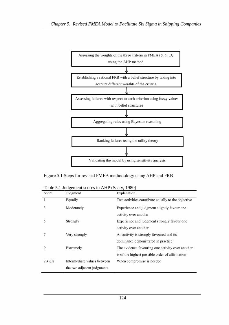
Chapter 5. Revised FMEA Model to Facilitate Six Sigma in Shipping Companies
124
Figure 5.1 Steps for revised FMEA methodology using AHP and FRB
Table 5.1 Judgement scores in AHP (Saaty, 1980) Score Judgment Explanation
1 Equally Two activities contribute equally to the objective
3 Moderately Experience and judgment slightly favour one
activity over another
5 Strongly Experience and judgment strongly favour one
activity over another
7 Very strongly An activity is strongly favoured and its
dominance demonstrated in practice
9 Extremely The evidence favouring one activity over another
is of the highest possible order of affirmation
2,4,6,8 Intermediate values between
the two adjacent judgments
When compromise is needed
Assessing the weights of the three criteria in FMEA (S, O, D)
using the AHP method
Establishing a rational FRB with a belief structure by taking into
account different weights of the criteria.
Aggregating rules using Bayesian reasoning
Assessing failures with respect to each criterion using fuzzy values
with belief structures
Ranking failures using the utility theory
Validating the model by using sensitivity analysis

Chapter 5. Revised FMEA Model to Facilitate Six Sigma in Shipping Companies
125
Step 2: Normalize the decision matrix and calculate the priorities of this matrix to
obtain the weights of criteria 𝑤𝑆 𝑤𝑂 𝑎𝑛𝑑 𝑤𝐷.
In order to calculate the weight of each criterion, the comparison matrix has to be
normalized. This can be done by summing each set of column values; then each
value is divided by the corresponding summed value. The relative weights of criteria
𝑤𝑆 𝑤𝑂 and 𝑤𝐷 are obtained through averaging each row. This can be presented by
using Equation (5.2).
𝑤𝑘 1
𝑛∑
𝑎𝑘𝑗
∑ 𝑎𝑖𝑗𝑛𝑖=
𝑛
𝑗=
𝑘 1 2 3 (5.2)
where, 𝑎𝑖𝑗 is the entry of row i and column j in a comparison matrix of order n and
𝑤𝑘 is the weight of a specific criterion k in the pairwise comparison matrix. In this
case, criterion 1 is S, 2 refers to O and 3 stands for D. The number of criteria /
alternatives in the matrix, 𝑛 3.
Step 3: Consistency check
In order to derive meaningful weights, a minimal consistency is required and a test
must be done. The consistency of the comparison matrices is tracked by a
Consistency Ratio (CR). CR index in AHP is used in order to maintain consistency
in decision making of the responders. CR can be defined as follows:
𝐶𝑅 𝐶𝐼
𝑅𝐼 (5.3)
CI is the consistency index and RI is the random index. CI can be defined as follows:
𝐶𝐼 𝜆𝑚𝑎𝑥 − 𝑛
𝑛 − 1 (5.4)

Chapter 5. Revised FMEA Model to Facilitate Six Sigma in Shipping Companies
126
where λmax defined as the largest eigenvalue is approximately calculated in Equation
(5.5).
𝜆𝑚𝑎𝑥
∑∑ 𝑤𝑘𝑎𝑗𝑘
𝑛𝑘=
𝑤𝑗
𝑛𝑗=
𝑛 𝑗 1 2 3 𝑘 1 2 3
(5.5)
where 𝑤𝑗 and 𝑤𝑘 are the weights of criteria obtained in Step 2.
RI is generated by Saaty’s team and the values are shown in Table 5.2. According to
Saaty (1995), the consistency ratio (CR) should be less than 5%, 8%, and 10% for a
3 × 3 matrix, a 4 × 4 matrix, and matrices of higher orders, respectively. If the CR
value is too high, then it is deemed that there is no reliability in the decision on the
chosen preference (Saaty, 1980).
Table 5.2 Random index (RI) for the factors used in the decision making process.
n 1 2 3 4 5 6 7 8 9 10
RI 0 0 0.58 0.9 1.12 1.24 1.32 1.41 1.45 1.49
5.3.2 Establishing a FRB with a Rational Belief Structure
In this method, both the three criteria and risk level are defined on the same plane of
a grade set of {very low, low, average, high, very high} and relevant weights are
assigned to the three criteria. The belief degrees associated with each grade of the
risk level for all rules are then calculated by using Equation (5.6).
𝛽𝑅𝑖𝑗
𝛽𝑆𝑖𝑗∙ 𝑤𝑆 + 𝛽𝑂𝑖
𝑗∙ 𝑤𝑂 + 𝛽𝐷𝑖
𝑗∙ 𝑤𝐷 (5.6)
where i = (1, 2, …, 5) means a grade in the set of {very low, low, average, high, very
high}; j is the jth rule in the rule base; 𝛽𝑇𝑖𝑗
(T (S, O, D)) equals one when Ti is
presented in the jth rule and otherwise it is zero. Consequently, the development of
the rule base with a belief structure can be standardised and rationalised. For

Chapter 5. Revised FMEA Model to Facilitate Six Sigma in Shipping Companies
127
example, a particular rule can be developed as follows.
Rule 2: IF S is very low, O is very low and D is low, THEN the risk level is very low
with a belief degree of “(wS+wO)”, low with a belief degree of “ wD”, average with
a belief degree of “0”, high with a belief degree of “0” and very high with a belief
degree of “0”.
By using Equation (5.6), the FRB with belief structures together with the weights of
FMEA criteria can be established as shown in Table 5.3.
Table 5.3 FRB with belief structures and weights of criteria in FMEA
By doing so, the complex work of constructing fuzzy rule bases with belief
structures in FMEA can be replaced through establishing relatively straightforward
linear calculation. This generic method is examined by a case study of failure
prioritisation of accounting management of a shipping line in Section 5.4.
5.3.3 Assessment of Failures Using Fuzzy Belief Structures
The three criteria (S, O, D) for every failure mode can be evaluated numerically or
Rules Antecedent attributes Risk Level
Severity of
failure (S)
Frequency of
occurrence (O)
Difficulty of
detection (D)
Very Low Low Average High Very High
Weight 𝑤𝑆 𝑤𝑂 𝑤𝐷 𝛽𝑅 𝛽𝑅 𝛽𝑅3 𝛽𝑅4 𝛽𝑅5
1 Very low Very low Very Low
𝑤𝑆 + 𝑤𝑂
+ 𝑤𝐷 0 0 0 0
2 Very low Very low Low
𝑤𝑆 + 𝑤𝑂 𝑤𝐷 0 0 0
3 Very low Very low Average 𝑤𝑆 + 𝑤𝑂 0 𝑤𝐷 0 0
… … … … … … … …
123 Very high Very high Average
0 0 𝑤𝐷 0 𝑤𝑆 + 𝑤𝑂
124 Very high Very high High 0 0 0 𝑤𝐷 𝑤𝑆 + 𝑤𝑂
125 Very high Very high Very high 0 0 0 0 𝑤𝑆 + 𝑤𝑂
+ 𝑤𝐷

Chapter 5. Revised FMEA Model to Facilitate Six Sigma in Shipping Companies
128
linguistically. Both of them have been extensively applied and have their merits and
demerits. However, the evaluation involves a high level of uncertainty since it is a
group decision behaviour and the assessment information for risk factors mainly
based on experts’ subjective judgments may be incomplete and imprecise. In
addition, many experts are willing to express their opinions by belief degrees (or
possibility measures) based on a set of evaluation grades, i.e., {Very Low, Low,
Moderate, High, and Very High} in reality (Liu et al., 2011), when no any single
grade can be individually used to describe risk parameters by them with full
confidence. From Section 5.3.2, it is known that the linguistic terms used to describe
variables (𝑇𝑖 , T (S, O, D); i=1, 2, …, 5), are set as “Very low”, “Low”,
“Average”, “High”, and “Very high”. The risk level of a particular failure is also
described using such linguistic variables (𝑅𝑖, i = 1, …, 5) as “Very low”, “Low”,
“Average”, “High”, and “Very high”. Each grade associated with the three criteria
can be described with respect to real observations. Furthermore, based on the
experts’ opinions, it is possible to represent all the five individual assessment grades
by trapezoidal fuzzy numbers. To simplify the discussion and without loss of
generality, their membership function values are developed based on Liu et al.
(2011)’s work (Figure 5.2 and Table 5.4). It is obviously possible to have some
flexibility in the definition of membership functions to suit different situations.
Membership
Figure 5.2 Fuzzy membership functions for linguistic terms
Very Low Low Average High Very High
1 2 3 4 5 6 7 8 9 10
1.0

Chapter 5. Revised FMEA Model to Facilitate Six Sigma in Shipping Companies
129
Table 5.4 Fuzzy ratings for linguistic terms.
Linguistic terms Fuzzy number
Very Low (1, 1, 2, 3)
Low (2, 3, 4, 5)
Average (4, 5, 6, 7)
High (6, 7, 8, 9)
Very High (8, 9, 10, 10)
Subjective judgements from Six Sigma project teams can then be collected using the
linguistic terms with belief degrees or any utility values. For example, the “O” of one
failure mode is judged by k experts as “𝑂𝑖” with 𝛽𝑂𝑖𝑛 belief degrees. Then the belief
degree of O belonging to 𝑂𝑖 is calculated as follows.
𝛽𝑂𝑖 ∑ 𝛽𝑂𝑖
𝑛𝑘𝑛=
𝑘 𝑛 1 2 . . 𝑘 𝑖 1 2 5 (5.7)
In the same way, the belief degree for S and D at different grades (i) evaluated by k
experts can be calculated by using Equation (5.8).
𝛽𝑇𝑖 ∑ 𝛽𝑇𝑖
𝑛𝑘𝑛=
𝑘 𝑛 1 2 . . 𝑘 𝑖 1 2 5 T 𝑆 𝑂 𝐷 (5.8)
It may sometimes be difficult for the experts to directly give the evaluations using
linguistic terms. If the evaluation is presented as other forms such as (i) a crisp
numerical value, (ii) a range of numerical value, (iii) a triangular fuzzy number and
(iv) a trapezoidal fuzzy number, it can be converted into linguistic terms with fuzzy
memberships using fuzzy mapping techniques such as the fuzzy similarity
calculation (Yang et al., 2009). Let 𝑢𝐸 be the fuzzy membership functions of a fuzzy
estimation E and 𝑢𝑇𝑖 (T (S, O, D); i=1, 2, …, 5) be the trapezoidal fuzzy numbers
of linguistic terms 𝑇𝑖, respectively. The similarity degrees between 𝑢𝐸 and 𝑢𝑇𝑖 can be
calculated as follows (Li and Liao, 2007).

Chapter 5. Revised FMEA Model to Facilitate Six Sigma in Shipping Companies
130
dx)(
dx)}(),(min{),(
xu
xuxuuuS
E
TE
TE
i
i (5.9)
If two membership functions are the same, that is 𝑢𝐸 𝑢𝑇𝑖, then 𝑆(𝑢𝐸 𝑢𝑇𝑖
) 1. If
two membership functions do not have any overlap, the similarity degree is zero. For
other situations, the higher the percentage of the overlap is, the higher the similarity
degree. After all the similarity degrees between and 𝑢𝑇𝑖 are computed, the belief
degree 𝐵𝑇𝑖, can be computed as follows:
𝐵𝑢𝐸
𝑇𝑖 𝑆(𝑢𝐸 𝑢𝑇𝑖
)
∑ 𝑆(𝑢𝐸 𝑢𝑇𝑖)5
𝑖=1
(T (S, O, D); i=1, 2, …, 5) (5.10)
For example, the similarity degree between a fuzzy estimation 𝑢𝐸 and 𝑢𝑇𝑖 (T (S,
O, D); i=1, 2, …, 5) in Figure 5.3 is calculated by using Equation (5.9) as follows:
𝑆(𝑢𝐸 𝑢𝑇1) 0
𝑎𝑟𝑒𝑎 +𝑎𝑟𝑒𝑎 +𝑎𝑟𝑒𝑎 3+𝑎𝑟𝑒𝑎 4 0
𝑆(𝑢𝐸 𝑢𝑇2) 𝑎𝑟𝑒𝑎 +𝑎𝑟𝑒𝑎
𝑎𝑟𝑒𝑎 +𝑎𝑟𝑒𝑎 +𝑎𝑟𝑒𝑎 3+𝑎𝑟𝑒𝑎 4 0.33
𝑆(𝑢𝐸 𝑢𝑇3) 𝑎𝑟𝑒𝑎 +𝑎𝑟𝑒𝑎 3
𝑎𝑟𝑒𝑎 +𝑎𝑟𝑒𝑎 +𝑎𝑟𝑒𝑎 3+𝑎𝑟𝑒𝑎 4 0.75
𝑆(𝑢𝐸 𝑢𝑇4) 0
𝑎𝑟𝑒𝑎 +𝑎𝑟𝑒𝑎 +𝑎𝑟𝑒𝑎 3+𝑎𝑟𝑒𝑎 4 0
𝑆(𝑢𝐸 𝑢𝑇5) 0
𝑎𝑟𝑒𝑎 +𝑎𝑟𝑒𝑎 +𝑎𝑟𝑒𝑎 3+𝑎𝑟𝑒𝑎 4 0
Furthermore, using Equation (5.10), 𝐵𝑢𝐸
𝑇𝑖 can be normalised as follows:
𝐵𝑢𝐸
𝑇1 𝑆(𝑢𝐸 𝑢𝑇1)
∑ 𝑆(𝑢𝐸 𝑢𝑇1)5𝑖=1
0
𝐵𝑢𝐸
𝑇2 𝑆(𝑢𝐸 𝑢𝑇2)
∑ 𝑆(𝑢𝐸 𝑢𝑇2)5𝑖=1
0.31
𝐵𝑢𝐸
𝑇3 𝑆(𝑢𝐸 𝑢𝑇3)
∑ 𝑆(𝑢𝐸 𝑢𝑇3)5𝑖=1
0.69
Eu

Chapter 5. Revised FMEA Model to Facilitate Six Sigma in Shipping Companies
131
𝐵𝑢𝐸
𝑇4 𝑆(𝑢𝐸 𝑢𝑇4)
∑ 𝑆(𝑢𝐸 𝑢𝑇4)5𝑖=1
0
𝐵𝑢𝐸
𝑇5 𝑆(𝑢𝐸 𝑢𝑇5
)
∑ 𝑆(𝑢𝐸 𝑢𝑇5)5
𝑖=1
0
Figure 5.3 Example of similarity degree between 𝑢𝐸 and 𝑢𝑇𝑖(T (S, O, D); i=1,
2, …, 5)
In this way, the fuzzy estimation for E can be transformed into the belief structure
and shown in the following form:
𝑢𝐸 = {(0, “Very Low”), (0.31, “Low”), (0.69, “Average”), (0, “High”), (0, “Very
High”)}
Consequently, raw data regarding the failure evaluation with respect to each criterion
can be presented in various formats to avoid useful information loss at an initial
stage. The obtained belief degrees can be converted and presented as the subjective
probabilities of a failure as:
𝑝 𝑇𝑖 𝛽𝑇𝑖 (5.11)
5.3.4 Rule Aggregation with the Weights of FMEA Criteria Using Bayesian
Reasoning
The principle of the FurBaR approach is used in this step. The kernel of the approach
is to appropriately transform belief degrees in rule bases into subjective conditional
𝑢𝑇1 𝑢𝑇2
𝒖𝑬 𝑢𝑇3 𝑢𝑇4 𝑢𝑇5
1 2 3 4 5 6 7 8 9 10
2
1
4
3
1.0

Chapter 5. Revised FMEA Model to Facilitate Six Sigma in Shipping Companies
132
probabilities in BN. The transformation makes it possible to take the advantages of
both fuzzy and Bayesian inference. Taking rule 2 in Table 5.3 FRB with belief
structures and weights of criteria in FMEA as an example, it can be symbolised as:
IF 𝑆 𝑆 𝑂 𝑂 and 𝐷 𝐷 , THEN 𝑅 (𝑤𝑆 +𝑤𝑂 ), 𝑅 𝑤𝐷 , 𝑅3 0 , 𝑅4 0 and
𝑅5 0.
It can be further transformed and presented by conditional probabilities as:
𝑝 𝑅𝑖|𝑆 𝑂 𝑎𝑛𝑑𝐷 𝑤𝑆 + 𝑤𝑂 𝑤𝐷 0 0 0 (5.12)
Using a BN technique, the FRB constructed in FMEA can be modelled and
converted into a four-node converging connection. It includes three parent nodes,
NO, NS, and ND (Nodes O, S and D); and one child node NR (Node R) (Yang et al.,
2008). Having transferred the rule base into a BN framework (see Equation (5.12)),
the rule-based risk inference for the failure criticality analysis will be simplified as
the calculation of the marginal probability of the node NR. The rule base in Table 5.3
denotes a 5555 conditional probability table (CPT) (see Table 5.5).
Table 5.5 The Conditional Probability Table of NR
S 𝑆
…
𝑆5
O 𝑂
…
𝑂5 𝑂
…
𝑂5
D
R 𝐷
…
𝐷5 𝐷
…
𝐷5 𝐷
…
𝐷5 𝐷
…
𝐷5
𝑅 𝑤𝑠 +
𝑤𝑂 + 𝑤𝐷 𝑤𝑆 + 𝑤𝑂
𝑤𝑆 +𝑤𝐷
𝑤𝑆 𝑤𝑂 +𝑤𝐷
𝑤𝑂 𝑤𝐷 0
𝑅 0 0 0 0 0 0 0 0
𝑅3 0 0 0 0 0 0 0 0
𝑅4 0 0 0 0 0 0 0 0
𝑅5 0 𝑤𝐷 𝑤𝑂 𝑤𝑂 +𝑤𝐷
𝑤𝑆 𝑤𝑆 +𝑤𝐷
𝑤𝑆 +𝑤𝑂
𝑤𝑆 + 𝑤𝑂
+ 𝑤𝐷
Subjective probabilities for each node of NO, NS and ND are expressed as p(𝑂𝑖), p(𝑆𝑗),
and p(𝐷𝑘) using Equation (5.11) respectively. Having analysed all the probabilities
of the four nodes, the probability of NR can be calculated as (Jensen, 2001):

Chapter 5. Revised FMEA Model to Facilitate Six Sigma in Shipping Companies
133
𝑝 𝑅ℎ ∑∑∑𝑝 𝑅ℎ|
5
𝑘=
5
𝑖=
5
𝑗=
𝑆𝑗 𝑂𝑖 𝐷𝑘 𝑝(𝑆𝑗)𝑝 𝑂𝑖 𝑝 𝐷𝑘 ℎ 1 5 (5.13)
where h, i, j and k all represent evaluation grades.
5.3.5 Failure Ranking
In order to prioritize failures, the appropriate utility values 𝑈𝑅ℎ for 𝑅ℎ ℎ 1 5
need to be assigned using the utility theory. They can be obtained by using the
centroid defuzzification method (Mizumoto, 1995). Consequently, the utility values
of 𝑅ℎ ℎ 1 5 can be calculated as below.
𝑈𝑅 = Very low = 1.778
𝑈𝑅 = Low = 3.5
𝑈𝑅3 = Average = 5.5
𝑈𝑅4 = High = 7.5
𝑈𝑅3 = Very high = 9.222
Then the failure priority/ranking index can be developed as:
𝑅𝐼 ∑𝑝 𝑅ℎ 𝑈𝑅ℎ
5
ℎ=
(5.14)
where the smaller the value of RI is, the lower the risk level of the potential failure
mode. The effects (EI) to RI values when input changes can be computed as:
𝐸𝐼 𝑅𝐼′ − 𝑅𝐼 ∑𝑝 𝑅ℎ
5
ℎ=
′𝑈𝑅ℎ − ∑𝑝 𝑅ℎ
5
ℎ=
𝑈𝑅ℎ (5.15)
where 𝑅𝐼′ and 𝑝 𝑅ℎ ′ represent the 𝑅𝐼 value and the probability of NR after changes
of inputs, respectively.

Chapter 5. Revised FMEA Model to Facilitate Six Sigma in Shipping Companies
134
The calculation process can be simplified by using a Hugin software package
(Andersen et al., 1990).
5.3.6 Validation
Validation is an important aspect of this methodology. It requires a careful test to
ensure its soundness. It is particularly important and desirable when subjective
elements are involved in the proposed methodology. In this study, sensitivity
analysis for partial validation of the model has been developed. If the methodology
is sound and its inference reasoning is logical, then the sensitivity analysis must at
least follow the following three axioms (Yang et al., 2008; Jones et al., 2010).
Axiom 1. A slight increment/decrement in the degrees of belief associated with any
linguistic variables of the three criteria will certainly result in the effect of a relative
increment/decrement in the degrees of belief of the linguistic variables of the Risk
Level.
Axiom 2. Given the same variation of belief degree distributions of the three criteria,
its influence magnitude to the Risk Level will keep consistency with their weight
distributions.
Axiom 3. The total influence magnitudes of the combination of the probability
variations from x criteria (evidence) on the values should always be greater than the
one from the set of x-y (y x) criteria (sub-evidence).
5.4 A Case Analysis of Accounting Management in Shipping Lines
In this section, the new FMEA method is illustrated through the failure analysis
process in a Six Sigma project for improving the accounting management of a world
leading container shipping company. It aims at reducing the amount of unmatched

Chapter 5. Revised FMEA Model to Facilitate Six Sigma in Shipping Companies
135
payment for non-credit customers. The project has followed the DMAIC
methodology and FMEA is used in the measure phase to identify failures of high
risk.
There are generally two types of customers in accounting in shipping lines’
operations: credit customer and non-credit customer. Credit customers are given the
right to make a lump sum payment for the service received from the shipping
company within a certain period (e.g. every 30 days). Non-credit customers are
required to make payments for every service before completion (delivery or release
of containers). It is found that very often the payments made by non-credit customers
cannot be or are wrongly allocated to the service provided. This has led to delays,
reworks and sometimes, loss of payments. Prior to the introduction of Six Sigma,
although much effort was put in to reduce the amount of unmatched payment,
continuous errors occurred without a systemic examination of relevant work
processes. The effort turned out to be insufficient. A Six Sigma project team of 4
members from both accounting and operational departments in a shipping company
was formed and led by this research. They include two senior managers and two
operational supervisors from different operational departments. At the early stage of
the measure phase, three process steps were identified, namely, “Charge input”,
“Invoice sending” and “Instruction from customers”. From the three steps, the
project team identified ten failure modes for key process inputs which are shown in
Table 5.6. The presented FMEA method in this work was then used to identify the
failure modes with high risk scores.
5.4.1 Establish a Pair-wise Comparison Decision Matrix and Calculate the
Weight for Each Criterion
A brainstorming technique was used to evaluate the relative pair-wise comparison
scores of the three criteria (S, O and D) from the team. The aggregate pair-wise
comparison matrix is established in Table 5.7. The weight of each criterion is then
calculated using Equation (5.2). The consistency of the judgements is checked. CR

Chapter 5. Revised FMEA Model to Facilitate Six Sigma in Shipping Companies
136
of the aggregate pair-wise comparison matrix is 0.0158 (below 5%), indicating a
satisfactory degree of consistency (Table 5.7).
Table 5.6 Failure modes identified
No of
Failures
Key Process Input Failure Modes
1 Experience level of operator inexperienced operator
2 Accurate quotation wrong quotation
3 Wellbeing of operator not well / personal problems
4 Clear information from port of loading (POL) late/no information from POL
5 Working machine fax machine break down
6 Volume of work of operator too much work to do
7 Time of sending request request sent after payment
8 Working machine system break down
9 Accurate information from customers wrong information from customer
10 Accurate tariff wrong tariff
Table 5.7 Comparison matrix for FMEA criteria
S O D 𝑤𝑖
S 1 1.5 2 0.454
O 0.67 1 2 0.347
D 0.5 0.5 1 0.199
𝜆𝑚𝑎𝑥 3.018 𝐶𝐼 0.0091 𝐶𝑅 0.0158
5.4.2 Rule Establishment with a Rational Belief Structure
The belief degrees relating to each rule have been calculated using Equation (5.6). It
is then further transformed into a subjective probability form using Equation (5.12).
Consequently, a new rule base with a rational belief structure by taking into account
different weights of the FMEA criteria is established and expressed in Table 5.8. The
completed rule base is presented in Appendix 3.

Chapter 5. Revised FMEA Model to Facilitate Six Sigma in Shipping Companies
137
Table 5.8 Sample of a new FMEA rule base with a rational belief structure
Failure S O D Risk Level
45.4% 34.7% 19.9% VL L A H VH
F1 VL VL VL 100.00% 0.00% 0.00% 0.00% 0.00%
F2 VL VL L 80.10% 19.90% 0.00% 0.00% 0.00%
F3 VL VL A 80.10% 0 19.90% 0 0
F4 VL VL H 80.10% 0 0 19.90% 0
F5 VL VL VH 80.10% 0 0 0 19.90%
F6 VL L VL 65.30% 34.70% 0 0 0
… … … … … … … … …
F123 VH VH A 0.00% 0.00% 19.90% 0.00% 80.10%
F124 VH VH H 0.00% 0.00% 0.00% 19.90% 80.10%
F125 VH VH VH 0.00% 0.00% 0.00% 0.00% 100.00%
5.4.3 Use Subjective Judgements to Estimate the Failure Modes
To facilitate the failure evaluation data collection, the meaning of each
grade/linguistic term used to describe the three FMEA criteria is defined in Table
5.9. It is noted that the numerical ranking values can be used to collect crisp
estimations from the team members. The members participated in identifying the
process inputs and assessing them against each criterion (S, O, D). Each member
provided his/her individual assessment to the failure modes against each criterion.
Four types of evaluations were received, including a single crisp number, a triangular
fuzzy number, a trapezoidal fuzzy number and an interval. Taking one failure mode
“inexperienced operator” as an example, the evaluations given by four members are
listed in Table 5.10. The evaluations were then transferred to linguistic terms with
belief degrees by using Equations (5.9) and Equation (5.10). The final belief degrees
for each risk level of this failure were calculated by using Equation (5.8) in Table
5.11. As each member plays the same role in the process and they had similar
working background, an equal weight was given to them in this study.

Chapter 5. Revised FMEA Model to Facilitate Six Sigma in Shipping Companies
138
Table 5.9 Ratings for S, O and D.
Rank Grade S O D
10 Very
high
Hazardous without
warning Failure is almost
inevitable
Cannot detect
9 Hazardous with warning Very remote chance of
detection
8
High
Loss of primary function
Repeated failures
Remote chance of
detection
7 Reduced primary function
performance
Very low chance of
detection
6
Average
Loss of secondary function Occasional
failures
Low chance of detection
5 Reduced secondary
function performance
Moderate chance of
detection
4
Low
Minor defect noticed by
most
customers Relatively few
failures
Moderately high chance
of detection
3 Minor defect noticed by
some customers High chance of detection
2
Very low
Minor defect noticed by
discriminating customers Failure is unlikely
Very high chance of
detection
1
Almost certain detection No effect
Table 5.10 Expert subjective input for S, O and D
S O D
Exp. 1 (6, 7, 8) (6, 7, 8) (6, 7, 8)
Exp. 2 100% High 50% High, 50% Av. 100% High
Exp. 3 (6, 7, 8) ( 5, 6, 7) (6, 7, 8)
Exp. 4 50% High, 50% Av. 100% Av. 100% High
Table 5.11 Belief degrees transformed from expert evaluations
S O D
Exp. 1 (0, 0, 0.2, 0.8, 0) (0, 0, 0.2, 0.8, 0) (0, 0, 0.2, 0.8, 0)
Exp. 2 (0, 0, 0, 1, 0) (0, 0, 0.5, 0.5, 0) (0, 0, 0, 1, 0)
Exp. 3 (0, 0, 0.2, 0.8, 0) (0, 0, 0.2, 0.8, 0) (0, 0, 0.2, 0.8, 0)
Exp. 4 (0, 0, 0.5, 0.5, 0) (0, 0, 1, 0, 0) (0, 0, 0, 1, 0)
Final BD 𝑝(𝑆𝑗) 0 0 0.225 0.775 0 𝑝 𝑂𝑖 0 0 0.475 0.525 0 𝑝 𝐷𝑘 0 0 0.1 0.9 0

Chapter 5. Revised FMEA Model to Facilitate Six Sigma in Shipping Companies
139
5.4.4 Conduct the Risk Inference
Having transformed evaluation into the format of probabilities, the risk level of “in-
experienced operator” can be calculated by using Equation (5.13) as:
𝑝 𝑅ℎ ∑ ∑ ∑ 𝑝 𝑅ℎ|5𝑘=
5𝑖=
5𝑗= 𝑆𝑗 𝑂𝑖 𝐷𝑘 𝑝(𝑆𝑗)𝑝 𝑂𝑖 𝑝 𝐷𝑘
𝑝 𝑅ℎ|𝑆3 𝑂3 𝐷3 𝑝 𝑆3 𝑝 𝑂3 𝑝 𝐷3 + 𝑝 𝑅ℎ|𝑆3 𝑂3 𝐷4 𝑝 𝑆3 𝑝 𝑂3 𝑝 𝐷4 +
𝑝 𝑅ℎ|𝑆3 𝑂4 𝐷3 𝑝 𝑆3 𝑝 𝑂4 𝑝 𝐷3 + 𝑝 𝑅ℎ|𝑆3 𝑂4 𝐷4 𝑝 𝑆3 𝑝 𝑂4 𝑝 𝐷4 +
𝑝 𝑅ℎ|𝑆4 𝑂3 𝐷3 𝑝 𝑆4 𝑝 𝑂3 𝑝 𝐷3 + 𝑝 𝑅ℎ|𝑆4 𝑂3 𝐷4 𝑝 𝑆4 𝑝 𝑂3 𝑝 𝐷4 +
𝑝 𝑅ℎ|𝑆4 𝑂4 𝐷3 𝑝 𝑆4 𝑝 𝑂4 𝑝 𝐷3 + 𝑝 𝑅ℎ|𝑆4 𝑂4 𝐷4 𝑝 𝑆4 𝑝 𝑂4 𝑝 𝐷4
0 0 1 0 0 × 0.225 × 0.475 × 0.1 + 0 0 0.801 0.199 0 × 0.225 × 0.475 × 0.9 +
0 0 0.653 0.347 0 × 0.225 × 0.525 × 0.1 + 0 0 0.454 0.546 0 × 0.225 × 0.525 × 0.9
+
0 0 0.546 0.454 0 × 0.775 × 0.475 × 0.1 + 0 0 0.347 0.653 0 × 0.775 × 0.475
× 0.9 +
0 0 0.199 0.801 0 × 0.775 × 0.525 × 0.1 + 0 0 0 1 0 × 0.775 × 0.525 × 0.9
= (0, 0, 0.287, 0.713, 0)
The result shows that the risk level associated with the failure mode “inexperienced
operator” is (0, 0, 0.287, 0.713, 0). It can be interpreted as that the risk level of
“inexperienced operator” is very low with a subjective probability of 0, low with a
subjective probability of 0, average with a subjective probability of 0.287, high with
a subjective probability of 0.713 and very high with a subjective probability of 0.
The above calculation can be modelled using Hugin software, which is a general
purpose tool for probabilistic graphical models such as Bayesian networks and
influence diagrams (Madsen et al., 2003). Taking the failure mode “inexperienced
operator” as an example, the risk level has been modelled as shown in Figure 5.4.

Chapter 5. Revised FMEA Model to Facilitate Six Sigma in Shipping Companies
140
Figure 5.4 Hugin example
5.4.5 Prioritization of the Failures
For the purpose of prioritization of the failures, the risk level expressed by linguistic
variables requires further analysis by assigning them appropriate utility values using
Equation (5.14). For example, the failure priority/ranking index for “inexperienced
operator” can be calculated as:
𝑅𝐼 ∑ 𝑝 𝑅ℎ 𝑈𝑅ℎ5ℎ=
0 × 1.788 + 0 × 3.5 + 0.287 × 5.5 + 0.713 × 7.5 + 0 × 9.222
6.93
In a similar way, the risk levels and RI values for all the other failure modes are
calculated and shown in Table 5.12. The result shows that the failure modes of the
highest risk levels are “inexperienced operator”, “request sent after payment” and
“too much work to do”. Thus, appropriate quality improvement measures can be
developed to reduce the unmatched payment effectively3.
3 This FMEA analysis was a part of a Six Sigma project for improving accounting management. The
final result from the project proved the cost effectiveness of the developed improvement measures

Chapter 5. Revised FMEA Model to Facilitate Six Sigma in Shipping Companies
141
Table 5.12 RI values for the failure modes identified
Failure Modes RI value Risk ranking
inexperienced operator 6.93 1
wrong quotation 6.14 4
not well / personal problems 6.03 6
late/no information from POL 6.06 5
fax machine break down 6.02 7
too much work to do 6.34 3
request sent after payment 6.52 2
system break down 5.47 9
wrong information from customer 5.71 8
Wrong tariff 5.45 10
Due to the fact that the failure modes identified in this FEMA study were the ones
related to key inputs that were screened by C&E matrix prior to the FMEA study, the
RI values are therefore close.
5.4.6 Validation of the Result
The accuracy of the result of the above analysis can be tested using sensitivity
analysis described in Section 5.3.6. First, it is required to clarify the relationship
between the risk levels of failure modes and the three criteria. The relationship, as
shown in Table 5.3, can be described as that the risk level is higher if the levels of its
S, O and D are higher. Next, a 10% (0.1) subjective probability is reassigned to each
criterion, and moved toward the increment/decrement of the risk level of a failure
mode. If the model reflects the logical reasoning, the risk level and RI values of the
mode should increase/decrease accordingly. For example, if the 10% subjective
probability of the Severity of the failure mode “in-experienced operator”
based on the successful identification of the failure modes of high risk levels.

Chapter 5. Revised FMEA Model to Facilitate Six Sigma in Shipping Companies
142
decreasingly moves from “High” to “Very low”, then the RI value of the failure
mode decreases from 6.93 to 6.18. Similar studies have been conducted for all the
other failure modes and all the results obtained are in line with Axiom 1 in Section
5.3.6.
From the above analysis, the effects of the minor input variation of the three criteria
reveal that the RI values (output) are sensitively changed in a logical manner.
However, the study does not well disclose the influence magnitude of the subjective
probability changes with reference to the weights of criteria. To investigate such an
influence magnitude, the change of a subjective probability with a step of 0.05 is
given to test the influence magnitude of the corresponding RI values for each
criterion. The result is observed and presented in a graphical form in Figure 5.5. It is
clearly seen that the influence magnitudes of the subjective probability changes of
each criterion to the RI values are significantly different and closely follow their
individual assigned weights. If the rule base structure is reliable, then the influence
magnitude to the RI values will follow the same weight ratio among the three criteria
S, O and D which is 9:7:4 (45.4% : 34.7% : 19.9%). For example, 0.05 subjective
probability changes from “High” to “Very low” in S, O and D for failure mode
“inexperienced operator” produce the effects to RI values as 0.13 (=6.93-6.80), 0.1
(=6.93-6.83) and 0.06 (=6.93-6.87), respectively. It shows that the influence
magnitude keeps harmony with the weight ratio. This is consistent with Axiom 2
introduced in Section 5.3.6.

Chapter 5. Revised FMEA Model to Facilitate Six Sigma in Shipping Companies
143
Figure 5.5 Sensitivity analysis
The rest of this section will analyse the effect of the combined variations from the
three criteria to RI values. The combinations of the variations can be categorised in
the following three groups.
1) Subjective probability variation of S, the subjective probability variation of O, and
the subjective probability variation of D.
2) The combination of the subjective probability variations of S and O, the
combination of the subjective probability variations of S and D, and the combination
of the subjective probability variations of O and D.
3) The combination of the subjective probability variations of S, O and D.
The tests for this investigation are carried out by changing subjective probabilities
for the failure mode of “inexperience operators” as an example. The change is 0.05
subjective probability variations from “High” to “Very Low” for all the criteria. The
results of RI and associated EI (using Equation (5.15)) are shown as follows.
1) Variations from individual criteria
0.13 (=6.93-6.81) for variation of S
0.1 (=6.93-6.83) for variation of O, and
0.06 (=6.93-6.87) for variation of D
0
0.2
0.4
0.6
0.8
1
1.2
1.4
0.05 0.1 0.15 0.2 0.25 0.3 0.35 0.4 0.45 0.5
EI (
Infl
ue
nce
mag
nit
ud
e t
o R
I)
Variation of subjective probability
S
O
D

Chapter 5. Revised FMEA Model to Facilitate Six Sigma in Shipping Companies
144
2) Variations from two criteria
0.23 (=6.93-6.7) from combination of S and O.
0.19 (=6.93-6.74) from combination of S and D.
0.16 (=6.93-6.77) from combination of O and D.
3) Variations of three criteria
0.29 (=6.93-6.64) from combination of S, O and D.
According to Axiom 3, if the model reflects the reality, then the influence magnitude
of the combined variations of the three criteria to RI values will always be greater
than the one of any two criteria, which in turn is greater than the one of each
individual criterion. Comparing all the relevant inference magnitudes to RI values
above (0.29 > any of (0.23, 0.19, 0.16), 0.29 > any of (0.13, 0.1, 0.06), 0.23> any of
(0.13, 0.1), 0.19> any of (0.13, 0.06) and 0.16> any of (0.1, 0.06)), it is clear that for
the investigation of this example, the model is sound. Furthermore, in a similar way,
more investigations are conducted to prove the reliability of the model in a
comprehensive manner.
5.5 Conclusion
FMEA is an important and popular tool used in Six Sigma. In view of its difficulties
in application in the shipping industry, a revised FMEA using FuRBaR approach is
proposed in this research. It can not only capture FMEA team members’ diverse
opinions under different types of uncertainties, but also consider the different
weights of the criteria of FMEA. In this approach, fuzzy logic is combined with
Bayesian reasoning in a complementary way where belief degrees are assigned to
subjective judgement of linguistic variables. The Bayesian marginalization algorithm
is used to conduct risk inference taking into considerations of the three criteria in
FMEA (S, O and D). It therefore, not only improves the accuracy of FMEA but also,
very importantly, maintains the easiness of FMEA.

Chapter 5. Revised FMEA Model to Facilitate Six Sigma in Shipping Companies
145
The application of the proposed FMEA method was examined and illustrated
through a real case study in a container shipping company. It showed that the
proposed method provided a practical, effective and flexible way for risk evaluation
in FMEA. For a particular unmatched payment scenario in accounting management,
it has been identified that the failure modes of the highest risk levels are “too much
work to do”, “inexperienced operator” and “request sent after payment”. The
proposed method also offers great potential to be applied in other industries,
especially those sectors in which failure data is unavailable or unreliable.

Chapter 6. Evaluating KPIs in Shipping Management by Using DEMATEL, ANP
and ER
146
Chapter 6. Evaluating KPIs in Shipping Management by
Using DEMATEL, ANP and ER
6.1 Introduction
Measuring performance in every aspect becomes an important part of today’s
business management. As one of the performance measurement instruments, KPIs
are widely used in practice as a freestanding tool or a part of process improvement
methodologies, such as Six Sigma.
KPIs are measures used to assess process performance in an organization which
provides useful information for measuring progress towards the company goals,
facilitating internal or external benchmarking and identifying inefficiencies in core
business operations. Well defined KPIs also enable an organization to be able to
measure the successes of projects and obtain data for future analysis.
It is found through the relevant literature review that KPIs are often defined as
quantitative measures (Ahmad and Dhafr, 2002; Bose, 2006; Cheng et al., 2011) and
those used in the service functions of shipping companies are mostly presented by
numerical data with a liner distribution. However, intangible performances with non-
liner distributions also need to be measured where quantitative KPIs become
inadequate, especially when human activities take a great part in the business
performance. In the service industries, the most important dimensions for quality
include: Time, Timelines, Completeness, Courtesy, Consistency, Accessibility and
Convenience, Accuracy and Responsiveness (Radovic et al., 2012). It is impossible
to define all of them by using quantitative measures. Furthermore, qualitative KPIs
can help managers to concentrate on an organisation’s objectives rather than what
can actually be measured. It is argued by many experienced consultants that an
Chapter 6. Evaluating KPIs in Shipping Management by Using DEMATEL, ANP
and ER
147
organization should deploy qualitative KPIs on starting a performance management
process and add quantitative ones over time as more information is gathered and the
process is being understood better. To measure qualitative performances, experts’
subjective judgements based on linguistic terms are often used, which inevitably
involve uncertainties and vagueness. It is difficult, if not impossible, to use a single
score or ratio for capturing imprecision and vagueness inherent in a subjective
assessment (Yang and Xu, 2002a). This is the main restriction for KPIs to be used
for measuring qualitative performance.
KPIs are commonly presented in a hierarchical structure with the lower level
indicators being grouped by their upper indicators or attributes (e.g. performance of
teams, tasks and functions, etc.) and all indicators are presumed to bear the same
weights without considering any interdependency in the evaluation process. In
reality, KPIs measure performances that carry different priorities to the business
objective. KPI accomplishment is a highly iterative process. It is common for
accomplishment of one KPI to cause extra cost or effort for other KPIs, due to
various reasons, such as incomplete information, limited resources, or
communication barriers. It is difficult but necessary to identify the inter-relationships
among different KPIs and the order of priorities for accomplishment of individual
KPIs (Cai et al., 2009). The management at a higher level makes decisions based on
the high level attribute(s) which is/are assessed through the associated lower level
indicators. In practice, qualitative data obtained from experts can be presented by
any given linguistic grades, such as, (good, bad) or (low, high). Even quantitative
data collected for KPIs may be measured in incomparable units, such as, “number of
staff trained” may be presented as “10 per month” and the “rate of wrong invoices”
could be “12%”. In order to use KPIs as an effective tool for benchmarking purposes,
outcomes from KPIs from different function areas or organizations need to be
presented in a comparable way, which means the KPIs need to be synthesized into
the same unit. It is commonly seen with quantitative KPIs that the average scores of
lower level KPIs are used to obtain value to measure their upper level KPIs’
performance in hierarchical structures. One of the drawbacks of scoring a subjective

Chapter 6. Evaluating KPIs in Shipping Management by Using DEMATEL, ANP
and ER
148
judgement as an average number is the possible loss of linkage between assessment
and business-planning activities in complex decision situations (Yang et al., 2001).
Furthermore, different indicators may have different priorities or importance in the
evaluation process, which is also affected by the existence of the interdependence
among them. For example, cost may be considered to be more important than safety
in the service functions of a shipping company, but the cost is affected by the safety.
As safety precautions and measurements increase due to the change of legislation,
the cost will increase. Therefore, to obtain a rational result from KPIs to assist
decision making, weights of indicators need be defined to reflect their priorities in
the whole system with consideration of interdependency among them, and the results
of KPIs can be transformed into compatible units. The lack of studies in this subject
has revealed a significant research gap to be filled.
This study therefore aims at developing a rigorous methodology for evaluating and
synchronizing both qualitative and quantitative KPIs. In this method, DEMATEL
and ANP methods are combined to produce the weights of indicators taking into
consideration the existence of interdependence. Fuzzy logic and Evidential
Reasoning (ER) are combined in a complementary way to synthesize both qualitative
and quantitative data. In order to achieve this purpose, the DEMATEL, ANP
methods and fuzzy ER approach are reviewed in section 2. The rest of the chapter is
organized as follows. Section 3 describes the development of the new research
methodology, followed by a case study in Section 4. Finally, the chapter is
concluded in Section 5.
6.2 Literature Review
6.2.1 KPIs in the Shipping Industry
In order to ensure that the predetermined goal of a company can be achieved,
monitoring is needed not only for the end results, but most importantly, inputs and
every step of each process. KPIs provide a useful tool to serve such a purpose for

Chapter 6. Evaluating KPIs in Shipping Management by Using DEMATEL, ANP
and ER
149
organizations. They are most commonly utilized to measure actual performances
against key success factors.
Shipping management has engaged in very limited systematic studies on
standardization of KPIs. KPIs are developed within an organization without industry
standardisation. Realizing the issue, InterManager initialized a shipping KPI project
aiming to develop a standard industry measurement tool. The project received a great
amount of support from the shipping industry. In 2011, shipping KPIs were officially
launched. The applications of the results from standardising the performance
measurements within the shipping industry are the Internal Improvement,
Benchmarking, Performance Based Contracting and Building of Public awareness
(Konsta and Plomaritou, 2012). However, all indicators identified have been
quantified even for the ones of qualitative features, crisp numbers are used for the
KPIs and average values are calculated to obtain final values. This method could
cause loss of information during data collection and make it difficult to reflect true
subjective evaluation in practice. Furthermore, the KPIs are not assigned associated
weights to reflect their importance, nor given any consideration of interdependence
within them which may have great impact on the outcome of final performance
evaluation.
6.2.2 DEMATEL
The DEMATEL method, developed by the Geneva Research Centre of the Battelle
Memorial Institute (Fontela and Gabus, 1976; Fontela and Gabus, 1973) is an
effective tool to model and quantify the causal relations within a set of criteria. It has
the ability to identify the interdependence among the factors within a system and
determine the level of interdependence between them. It has therefore been used in
many areas, to identify different factors for business needs (Shieh et al., 2010; Fan et
al., 2012), analyse interrelated relationships within business (Wang and Tzeng,
2012), select suppliers (Dey et al., 2012) and define relationships between KPIs
(Cheng et al., 2011).

Chapter 6. Evaluating KPIs in Shipping Management by Using DEMATEL, ANP
and ER
150
6.2.3 ANP
ANP is an attractive MCDM tool, which was proposed by Saaty in 1996. It is an
extension of Analytical Hierarchy Process (AHP) and allows the consideration of
interdependence among and between levels of attributes and alternatives. Different
from AHP, ANP uses a network without the need to specify levels as in hierarchy.
Figure 6.1 presents the differences between the structures of hierarchy and network.
Hierarchy structure is a special case of a network system where weights are
determined independently. ANP focuses on dependency among elements within the
same cluster (inner dependency) and between different clusters (outer dependency)
(Saaty, 2008) and provides a way to input judgments and measurements to derive
ratio scale priorities for the distribution of influences among the factors and groups
of factors in the decision. Outer dependence is the dependence between clusters but
in a way to allow for feedback circuits. Inner dependence is the interdependence
within a cluster combined with feedbacks between clusters (Saaty and Takizawa,
1986). ANP provides a tool to evaluate all the relationships systematically by adding
all interactions, interdependences, and feedbacks in decision making systems (Zaim
et al., 2014).
Figure 6.1 Hierarchy and Network
𝑒 𝑒 𝑒3
𝑒4 𝑒5 𝑒6
Cluster
Elements
Inner dependency
Outer dependency
Feedbacks
Attribute Attribute
𝑒 𝑒 𝑒3
𝑒4 𝑒5 𝑒6
Hierarchy Network
Chapter 6. Evaluating KPIs in Shipping Management by Using DEMATEL, ANP
and ER
151
ANP has been highly appreciated due to the fact that many decision problems cannot
be presented by a hierarchical structure because of the existence of interdependence.
Its application can be found in a wide range of areas, such as analysing
organizational project alternatives (Meade and Sarkis, 1999), R&D project selection
(Meade and Presley, 2002), supplier selection (Gencer and Guerpinar, 2007),
resource allocation in transportation (Wey and Wu, 2007), strategic e-business
decision analysis (Raisinghani et al., 2007) and many more. Literature also shows
that ANP has often been used together with DEMATEL to determine the influencing
weights for criteria (Chen, 2012; Vujanovic et al., 2012; Tsai and Hsu, 2010; Lee et
al., 2011).
KPIs in organizations are not independent but highly influencing and with feedback
relationships among them. The use of DEMATEL and ANP provides a path to
effectively evaluate the importance of indicators and address the existence of inter-
relationships. In an ANP method, not all indicators need to be pairwise compared,
but only those that have a non-zero influence. For the others that do not have any
interdependency, a zero value will be assigned. Therefore, the use of DEMATEL
performs an accurate initial assessment for the upper level KPIs to identify their
relationship of interdependency which can then be further narrowed down for the
ANP analysis.
6.2.4 Fuzzy Logic and Evidential Reasoning (ER) Algorithm
Fuzzy logic was designed to deal with fuzziness in data. It is mostly applied using
fuzzy IF-THEN rules (fuzzy rule-based system) derived from human knowledge. A
fuzzy rule-based system allows the modelling of language-related uncertainties by
providing a systematic procedure to transfer human knowledge and the reasoning
process without the need of precise quantitative analysis. It uses a collection of fuzzy
IF-THEN rules from human experts or domain knowledge and combines them into a
single system. Many studies have combined the fuzzy rule-based system with other
methodologies, such as neural network (Lin and Lee, 1991; Lee and Teng, 2000;

Chapter 6. Evaluating KPIs in Shipping Management by Using DEMATEL, ANP
and ER
152
Mitra and Hayashi, 2000), generic algorithms (Ishibuchi et al., 1995; Phillips et al.,
1996) and ER (Liu et al., 2004; Dymova et al., 2010) to take their combined
advantages in dealing with uncertainty.
ER is a process of drawing plausible conclusions from uncertain or incomplete
information (Yang et al., 2009b). It was developed based on Dempster-Shafer (D-S)
theory in 1994 for dealing with multiple attribute decision analysis (MADA)
problems (Yang and Singh, 1994). The kernel of the ER approach is an evidential
reasoning algorithm developed on the basis of a multi-attribute evaluation
framework and evidence combination rule of the D-S theory. The algorithm can be
used to aggregate attributes of a multilevel structure (Yang and Xu, 2002b). It has
been applied to many decision making problems, such as, vessel selection (Yang et
al., 2009b), organizational self-assessment (Yang et al., 2001), roadside hazard
severity indicator evaluation (Ayati et al., 2012) and general cargo ship design (Sen
and Yang, 1995).
FER combines the two approaches, fuzzy logic and ER. It has developed itself as an
established MADA method and is widely used to solve complex decision problems
in various applications. For example, Yang et al. (2009c) used FER to synthesize
evaluations for decision attributes in selecting security control options; Liu et al.
(2011) applied FER in capturing and aggregating the diversified, uncertain
assessment information given by team members during data collection for failure
mode and effects analysis. FER is therefore adopted in this study to synthesise KPI
evaluations in a meaningful way so that they can be confidently used to make
decisions.
6.3 KPIs Management in the Shipping Industry by Using
DEMATL, ANP and FER
The functionalities of KPIs can be fully utilized through systematic management.

Chapter 6. Evaluating KPIs in Shipping Management by Using DEMATEL, ANP
and ER
153
KPIs are indicators measuring performances that need to be measured without
considering the types of the data presenting them. A KPI tree is normally in a
hierarchical structure. The top levels contain the KPIs that can assist top
management to obtain a clear view of company overall performance and make
decisions. The sub-levels KPIs or PIs are those used to measure the performances
contributing to the attributes that are measured by the top level KPIs. A KPI tree
contains as many levels as necessary until it reaches a point where users are
confident to obtain and use adequate information or experience to provide the inputs
for the indicators. In order to assess performances confidently through KPIs, their
importance to the objective need to be determined and the information they provide
are to be transformed into compatible units and subsequently synthesised. This can
be achieved by the application of DEMATEL, ANP and FER methods. The
proposed framework is presented in Table 6.2 and described as below.
6.3.1 Identify KPIs and PIs to Build a KPI Tree
Putting performance measurement in place could be a time and effort consuming
task, especially when there is a lack of incentives and top management support.
Many service functions of shipping companies may already have a certain number of
indicators such as financial and sales indicators. There were no standard shipping
KPIs that have been widely adopted in the industry. The shipping KPI project
initiated by InterManager has provided an opportunity to develop standard industry
measurements. However, those indicators are mainly focusing on the measurement
of vessel operations instead of service functions. For shipping management
companies, it is a crucial task to identify indicators that can be used to effectively
measure their service performance.
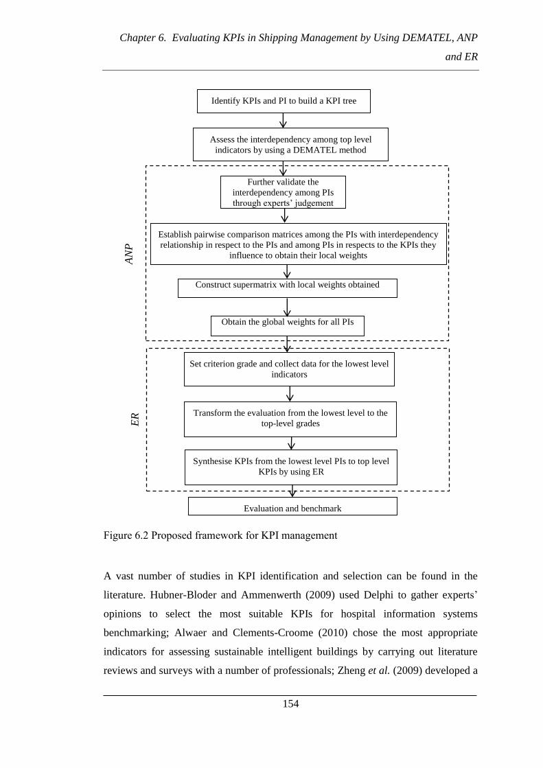
Chapter 6. Evaluating KPIs in Shipping Management by Using DEMATEL, ANP
and ER
154
Figure 6.2 Proposed framework for KPI management
A vast number of studies in KPI identification and selection can be found in the
literature. Hubner-Bloder and Ammenwerth (2009) used Delphi to gather experts’
opinions to select the most suitable KPIs for hospital information systems
benchmarking; Alwaer and Clements-Croome (2010) chose the most appropriate
indicators for assessing sustainable intelligent buildings by carrying out literature
reviews and surveys with a number of professionals; Zheng et al. (2009) developed a
Identify KPIs and PI to build a KPI tree
Assess the interdependency among top level
indicators by using a DEMATEL method
Set criterion grade and collect data for the lowest level
indicators
Transform the evaluation from the lowest level to the
top-level grades
Synthesise KPIs from the lowest level PIs to top level
KPIs by using ER
Evaluation and benchmark
Further validate the
interdependency among PIs
through experts’ judgement
Obtain the global weights for all PIs
Establish pairwise comparison matrices among the PIs with interdependency
relationship in respect to the PIs and among PIs in respects to the KPIs they
influence to obtain their local weights
Construct supermatrix with local weights obtained
AN
P
ER

Chapter 6. Evaluating KPIs in Shipping Management by Using DEMATEL, ANP
and ER
155
performance measurement indicator system by adopting a framework from previous
studies and validate the KPIs through surveys and interviews for technological
innovation of a firm; Cheng et al. (2011) applied the Delphi method to obtain KPIs
and their dimensions and mind map to draw a KPI framework for new product
development; McCance et al. (2012) identified KPIs for nursing and midwife care by
using workshop and consensus. All those methods can be used to effectively identify
indicators and construct KPI trees.
6.3.2 Assess the Interdependencies of the Top Level Indicators using
DEMATEL
The application of DEMATEL is to identify interdependencies among the top level
indicators to narrow down the amount of pairwise comparison that needs to be
conducted in the ANP method when prioritising KPIs. The method can be
summarized as follows:
Step 1: Compute the average matrix (M)
Suppose there are n indicators under the same objective or another indicator on a
KPI tree and there are G experts who provide evaluation of the direct influence
between any two indicators. Respondents are asked to indicate the degree of direct
influence one indicator i exerts on another indicator j. The evaluation is based on the
scale of 0, 1, 2, 3, 4, which represent “no influence”, “low influence”, “medium
influence”, “high influence” and “extremely high influence” respectively. A higher
score from a respondent indicates a belief that insufficient involvement in the
problem of indicator i exerts a stronger possible direct influence on the inability of
indicator j, or, in positive terms, that greater improvement in indicator i is required to
improve indicator j (Tzeng et al., 2007). The notation of 𝑥 𝑖𝑗 indicates the degree to
which the expert believes the ith indicator affects the jth indicator. For 𝑖 𝑗, the
diagonal elements are set to zero. A 𝑛 × 𝑛 matrix for the evaluation of each expert
(𝑥𝑖𝑗𝑔 can be established as 𝑋𝑔 [𝑥𝑖𝑗
𝑔], where g is the gth of the expert with 1 ≤ g

Chapter 6. Evaluating KPIs in Shipping Management by Using DEMATEL, ANP
and ER
156
≤G. Thus, 𝑋 , 𝑋 𝑋3…𝑋𝐺 are the matrices from G experts. The average matrix
𝑀 [𝑚𝑖𝑗] can be constructed as below.
𝑀 [𝑚𝑖𝑗] [
𝐺∑ 𝑥𝑖𝑗
𝑔𝐺𝑔= ] 𝑖 1 2 𝑛 , 𝑗 1 2 𝑛
Step 2: Normalize the average matrix (M) and obtain the normalized direct relation
matrix (D)
The normalized direct-relation matrix D can be obtained by equation (6.1).
𝐷 𝑀 × 𝑆 (6.1)
where 𝑆 𝑀𝑖𝑛[
𝑚𝑎𝑥1≤𝑖≤𝑛 ∑ 𝑚𝑖𝑗𝑛𝑗=1
𝑚𝑎𝑥1≤𝑖≤𝑛 ∑ 𝑚𝑖𝑗𝑛𝑖=1
] . Each element in matrix D falls
between zero and one.
Step 3: Calculate the total relation matrix (T)
The total relation matrix T is obtained by using Equation (6.2).
𝑇 [𝑡𝑖𝑗]𝑛×𝑛 lim
𝑚=∞ 𝐷 + 𝐷 + ⋯+ 𝐷𝑚
∑ 𝐷𝑖∞𝑚= 𝐷 𝐼 − 𝐷 −
(6.2)
where I is the identity matrix and total relation matrix can be presented as below.
[𝑡𝑖𝑗]𝑛×𝑛
[ 𝑡 ⋯ 𝑡 𝑗 ⋯ 𝑡 𝑛
⋮ ⋮ ⋮ ⋮𝑡𝑖 ⋯ 𝑡𝑖𝑗 ⋯ 𝑡𝑖𝑛
⋮ ⋮ ⋮ ⋮𝑡𝑛 ⋯ 𝑡𝑛𝑗 ⋯ 𝑡𝑛𝑛]
Step 4: Calculate the sums of rows and columns of the total relation matrix (T)
Let r and c be the sum of rows and sum of columns of the total relation matrix T,

Chapter 6. Evaluating KPIs in Shipping Management by Using DEMATEL, ANP
and ER
157
respectively. Suppose that 𝑟𝑖 represents the sum of ith row and 𝑐𝑗 denotes the sum of
jth column, then the value of 𝑟𝑖 indicates the effects given by indicator i to the other
indicators (Equation (6.3)) and 𝑐𝑗 shows effects received by indicator j from the
other indicators (Equation (6.4)) both directly and indirectly. When 𝑖 𝑗, the sum
𝑟𝑖 + 𝑐𝑗 illustrates the total effects given and received by indicator i, and 𝑟𝑖 − 𝑐𝑗
indicates the net effect that indicator i contributes to the system. 𝑟𝑖 + 𝑐𝑗 indicates
the degree of importance that factor i plays in the system. Moreover, if 𝑟𝑖 − 𝑐𝑗 is
positive, indicator i is a net cause, while indicator i is a net receiver or result if 𝑟𝑖 −
𝑐𝑗 is negative (Liou et al., 2007).
𝑟𝑖 ∑ 𝑡𝑖𝑗𝑛𝑗= 𝑖 1 2 . . 𝑛 (6.3)
𝑐𝑗 ∑ 𝑡𝑖𝑗𝑛𝑖= 𝑗 1 2 . . 𝑛 (6.4)
Step 5: Set threshold value (α) and obtain the impact relations-map (IRM).
Setting a threshold value (α) is to filter out those indicators that only have negligible
effects so that the indicators bearing considerable effects can be clearly identified for
effective decision making. Only factors with effect greater than the threshold value
should be chosen and shown in an impact-relations-map (IRM) or causal diagram
(Tang et al., 2007). The values that are lower than the threshold will be set to zero in
the total relation matrix (T). The threshold value can be obtained through either
subjective judgement from experts (Gwo-Hshiung et al., 2007) or mathematical
calculation (Wu and Tsai, 2012). The mathematical method is adapted to obtain the
threshold value in this study, which is calculated by the average value of 𝑡𝑖𝑗 in
matrix T (Equation (6.5))
𝛼 ∑ ∑ 𝑡𝑖𝑗
𝑛𝑗=1
𝑛𝑖=1
𝑁
(6.5)
where N is the total number of elements (𝑛 ∗ 𝑛) in the matrix T. Any value lower
than 𝛼 in matrix T is considered to be zero to construct the matrix 𝑇𝛼.

Chapter 6. Evaluating KPIs in Shipping Management by Using DEMATEL, ANP
and ER
158
The IRM is constructed and presents the relationship based on the matrix 𝑇𝛼 . The
IRM visualizes the interdependency relationship among indicators.
The same processes start with the top level indicators so that only those lower level
indicators which have been identified with the possibility of influencing or being
influenced by other indicators need to be further analysed.
6.3.3 Obtain Lower Level Indicator Weights by using the ANP Method
After the interdependencies among the top level indicators are identified by
DEMATEL, the indicators in the group of those top level indicators need to be
reviewed to identify the interdependency relationship among them. This can be done
by group discussion with experts. Through this activity, the lowest level indicators
with interdependency can be confirmed. ANP calculation can then be utilized to
analyse their interdependencies and obtain the local weights for indicators.
Step 1: Establish pairwise comparisons matrices (A) for all indicators and obtain
local weights
The relative importance values for all indicators with interdependencies need to be
obtained through pairwise comparisons. The pairwise comparison matrices are
constructed among the top level indicators and indicators under the same top level
indicator. The respondents need to answer the questions such as: “Given an indicator
and its upper level indicator or objective, which of the two indicators influences the
given indicator more with respect to the upper level indicator or objective, and how
much more than another indicator?”. The responses are presented numerically,
scaled on the basis of Saaty’s 1-9 scale where 1 presents indifference between the
two indicators and 9 stands for overwhelming dominance of the indicator under
consideration (row indicator) over the comparison indicator (column indicator) in a
pairwise comparison matrix. Suppose there are m indicators to be compared in a
matrix, let 𝑒 𝑒 𝑒𝑚 denote the different indicators, where 𝑎 𝑖𝑗 represents the

Chapter 6. Evaluating KPIs in Shipping Management by Using DEMATEL, ANP
and ER
159
level of influences that the respondent believes when indicator 𝑒𝑖 is compared with 𝑒𝑗.
When scoring is conducted for a pair, a reciprocal value is automatically assigned to
the reverse comparison within the matrix.
𝑒 𝑒 ⋯ 𝑒𝑗 ⋯ 𝑒𝑚
𝐴 𝑎 𝑖𝑗
𝑒 𝑒 ⋮𝑒𝑖⋮
𝑒𝑚 [ 𝑎 𝑎 ⋯ 𝑎 𝑗 ⋯ 𝑎 𝑚
𝑎 𝑎 ⋯ 𝑎 𝑗 ⋯ 𝑎 𝑚
⋮ ⋮ ⋮ ⋮ ⋮ ⋮𝑎𝑖 𝑎𝑖 ⋯ 𝑎𝑖𝑗 ⋯ 𝑎𝑖𝑚
⋮ ⋮ ⋮ ⋮ ⋱ ⋮𝑎𝑚 𝑎𝑚 ⋯ 𝑎𝑚𝑗 ⋯ 𝑎𝑚𝑚]
(6.6)
where 𝑎 𝑖𝑗 1 if 𝑖 𝑗; 𝑎 𝑖𝑗
𝑎𝑗𝑖 , 𝑖 1 2 𝑚 and 𝑗 1 2 𝑚
Once the pairwise comparisons are completed, the local priority vectors can be
obtained by dividing each element in a column by the sum of the column elements
and then summing the elements in each row of the resultant matrix and dividing by
the number of elements in the row (Meade and Sarkis, 1999). This is presented by
Equation (6.7).
𝑤𝑘
𝑚∑
𝑎𝑘𝑗
∑ 𝑎𝑖𝑗𝑛𝑖=1
𝑚𝑗= 𝑘 1 2 𝑚 (6.7)
where, 𝑤𝑘 is the priority vector of a specific indicator k in the pairwise comparison
matrix. Its value is a part of the supermatrix in the later steps.
Step 2: Form unweighted supermatrix
ANP uses supermatrix for a resolution of the effects of the interdependence that
exists between the elements of the system (Meade and Sarkis, 1999). The elements
of the supermatrix are imported from the pairwise comparison matrices of
interdependencies (step 1). A supermatrix with an example of one of its general entry
matrices is shown as Equation (6.8)

Chapter 6. Evaluating KPIs in Shipping Management by Using DEMATEL, ANP
and ER
160
𝐶 ⋯ 𝐶𝑗 ⋯ 𝐶𝑛
𝑒 ⋯𝑒 𝑚1
⋯ 𝑒𝑗 ⋯𝑒𝑗𝑚𝑗 ⋯ 𝑒𝑛 ⋯𝑒𝑛𝑚𝑛
𝑊
𝐶
𝑒 𝑒 ⋮
𝑒 𝑚1
⋮
𝐶𝑖
𝑒𝑖
𝑒𝑖
⋮𝑒𝑖𝑚𝑖
⋮
𝐶𝑛
𝑒𝑛
𝑒𝑛
⋮𝑒𝑛𝑚𝑛
[ 𝑊 ⋯ 𝑊 𝑗 ⋯ 𝑊 𝑛
⋮ ⋮ ⋮
𝑊𝑖 ⋯ 𝑊𝑖𝑗 ⋯ 𝑊𝑖𝑛
⋮ ⋮ ⋮
𝑊𝑛 ⋯ 𝑊𝑛𝑗 ⋯ 𝑊𝑛𝑛]
(6.8)
where 𝐶𝑛 denotes the nth cluster (top level indicator or objective), 𝑒𝑛𝑚 represents the
mth indicator in the nth cluster, and 𝑊𝑖𝑗 is the principal eigenvector of the influence
of the indicators in the jth cluster compared to the ith cluster. If jth cluster has no
influence on the ith cluster, then 𝑊𝑖𝑗 0. 𝑊𝑖𝑗 (Figure 6.3) represents the values of
priority vectors of indicators from the cluster 𝐶𝑖 in relation to elements from the
cluster 𝐶𝑗 which were derived from step 1.
𝑊𝑖𝑗 |
|
𝑤𝑖 𝑗
𝑤𝑖 𝑗
𝑤𝑖
𝑗𝑚𝑗
𝑤𝑖 𝑗
𝑤𝑖 𝑗
𝑤𝑖
𝑗𝑚𝑗
⋮ ⋮ ⋮ ⋮
𝑤𝑖𝑚𝑖
𝑗 𝑤𝑖𝑚𝑖
𝑗 𝑤
𝑖𝑚𝑖
𝑗𝑚𝑗
|
|
Figure 6.3 i, j block of a supermatrix in ANP
Step 3: Obtain weighted supermatrix
The weighted supermatrix can be obtained through multiplying the priority vectors
of each element in the un-weighted supermatrix with the priority vectors of the
corresponding clusters (both were calculated in step 1).

Chapter 6. Evaluating KPIs in Shipping Management by Using DEMATEL, ANP
and ER
161
Step 4: Calculate the global weights with the limiting supermatrix
The super-matrix is made to converge to obtain a long-term stable set of weights.
This is achieved by multiplying the weighted suprematrix itself multiple times to
obtain the limiting supermatrix (limiting weighted supermatrix). In other words, the
weighted supermatrix is raised to the kth power, where k is an arbitrarily large
number, until it becomes a stable supermatrix in order to obtain the global priority-
influential vectors, also called the global weights.
The lengthy and complex calculation of ANP can be eased by the use of the
computer software - “Super decisions”. By creating relationships among indicators
and inputting the original evaluations from the pairwise comparison matrices in the
software, the global weight can be obtained directly.
6.3.4 Set Criterion Grade and Collect Data for the Lowest Level Indicators
Before data collection, corresponding grades are required to be given to all indicators
for experts’ assessments using either objective data or subjective judgement. For
indicators with qualitative data input, various sets of linguistic terms are defined to
reflect the nature of the criteria. For example, a set of linguistic terms (Very satisfied,
satisfied, average, unsatisfied, extremely unsatisfied) can be used to categorize the
evaluation of the indicator “customer satisfaction”. For those indicators with
quantitative data, numerical grades can be used, For instance, the evaluation grades
for the percentage of late deliveries per week could be described as “Very poor” if
the rate is more than 20%, “Poor” if the rate is 15%, “Average” if the rate is 10%,
“Good” if the rate is 5% and “Very Good” if the rate is “0%”. The setting of the
grades can be based on experts’ opinion, historical data and/or organizations’
objectives/expectations. When utilizing historical data for the grade setting, values
for the two grades (i.e. the most and least prepared) need to be firstly determined
through the data available. The values for the most preferred rating and the least
preferred rating are represented by the best and worst records among the data. The

Chapter 6. Evaluating KPIs in Shipping Management by Using DEMATEL, ANP
and ER
162
grade setting can also be conducted by any other grade that is known or can be
determined, e.g. a target value or average value. Suppose there are N evaluation
grades to assign the numerical values to and the values for the already known two
grades are presented by 𝑣ℎ and 𝑣𝑙 , where 1 ≤ 𝑙 < ℎ ≤ 𝑁 . The values for the in-
between grades ( 𝑣𝑛 ) can then be calculated by using a linear distribution in
Equations (6.9) and (6.10).
𝑣𝑛 𝑣𝑛+ − (𝑣ℎ−𝑣𝑙
ℎ−𝑙) 𝑖𝑓𝑣𝑙 < 𝑣𝑛 < 𝑣ℎ 1 ≤ 𝑛 ≤ 𝑁 − 1 (6.9)
𝑣𝑛 𝑣𝑛− + (𝑣ℎ−𝑣𝑙
ℎ−𝑙) 𝑖𝑓 𝑣𝑙 > 𝑣𝑛 > 𝑣ℎ 2 ≤ 𝑛 ≤ 𝑁 (6.10)
6.3.5 Transform the Evaluation from the Lowest Level to Top Level Grades
Raw data collected for indicators could be in different formats and grades. In order
to execute further analysis and assessment, the grades defined need to be
transformed into the same form. The transformation is carried out by establishing
fuzzy rule bases based on experts’ experience and/or organization
objectives/expectations.
For example, assume that the indicator “Elapsed time between shipping instruction
& Bill of Lading issue” has its upper level indicator “Team performance” and top
level KPI “company competitiveness” in a KPI tree. The top level KPI “Company
competitiveness (C)” can be described linguistically in terms of “Very competitive
(C1)”, “Fairly competitive (C2)”, “Average (C3)” and “Not competitive (C4)”. The
indicator “Team efficiency (T)” can be expressed using linguistic terms as “Very
Good (T1)”, “Good (T2)”, “Average (T3)”, “Poor (T4)” and “Very poor (T5)”. The
linguistic terms used to assess the indicator “Elapsed time between shipping
instruction & Bill of Lading issue (E)” are “less than 2 days (E1)”, “3 days (E2)”, “4
days (E3)” and “more than 5 days (E4)”. A fuzzy rule base belief structure between
the linguistic terms expressing the indicators at three levels can be generated for the
transformation from fuzzy input to output as shown below.

Chapter 6. Evaluating KPIs in Shipping Management by Using DEMATEL, ANP
and ER
163
R1: IF “Elapsed time between shipping instruction & Bill of Lading issue (E)” is
“less than 2 days (E1)”, then “team performance (T)” is “Very Good (T1)” with
100% degree of belief.
It can be simplified as:
R1: IF E1, then 100% T1.
Similarly,
R2: IF E2, then75% T2 and 25% T3.
R3: IF E3, then 50% T3 and 50% T4.
R4: IF E4, then 25% T4 and 75% T5.
R5: IF T1, then 100% C1.
R6: IF T2, then 25% C1 and 75% C2.
R7: IF T3, then 15% C2 and 85% C3.
R8: IF T4, then 15% C3 and 85% C4.
R9: IF T5, then 100% C4.
Through this method, the “Elapsed time between shipping instruction & Bill of
Lading issue” can be transformed onto “Company competitiveness”. For example, if
the Elapsed time between shipping instruction & Bill of Lading issue for a company
is 4 days, according to R3, it can be described as 50% T3 and 50% T4. Based on R7
and R8, It can then be converted into (7.5% C2 and 42.5% C3) and (7.5% C3 and
42.5% C4), respectively. Consequently, it equals to 7.5% C2, 50% C3 and 42.5%
C4.
6.3.6 Synthesise Indicators from the Lowest Level PIs to Top Level KPIs by
using an ER Algorithm
Once the transformation from the lowest level to the top level indicators is
completed, the information can then be utilized in the ER algorithm which can be
explained as follows (Yang and Xu, 2002b).

Chapter 6. Evaluating KPIs in Shipping Management by Using DEMATEL, ANP
and ER
164
Suppose there is a two level hierarchy structure - a parent level KPI E consists of 𝐿
indicators at the children level which include all the indicators influencing the
assessment of the KPI E. Indicators can be represented as
𝐸 𝑒 𝑒 𝑒𝑖 𝑒𝐿 .
The weight of each indicator was obtained in section 6.3.3 and can be expressed as
𝑤 𝑤 𝑤 𝑤𝑖 𝑤𝐿 . 𝑤𝑖 is the normalized relative weight for indicator 𝑖 where
0≤𝑤𝑖≤1 and ∑ 𝑤𝑖𝐿𝑖= 1.
Let N present the number of evaluation grades, Each 𝐻𝑛 𝑛 1 2 𝑁 is a standard
grade for assessing an indicator for a top level KPI. Evaluations for all the indicators
obtained in section 6.3.4 were transformed to the standard grades through the
technique in section 6.3.5. Let 𝐴𝑖 represent the transformed evaluation for indicator
𝑒𝑖. The evaluations can then be presented as follows:
𝐴𝑖 [ 𝐻𝑛 𝛽𝑛 𝑖 𝑛 1 2 𝑁] (6.11)
where 𝛽𝑛 𝑖 is the degree of belief associated with the evaluation grade 𝐻𝑛 for the
indicator 𝑒𝑖 and ∑ 𝛽𝑛 𝑖𝐿𝑖= ≤ 1 . When all 𝐻𝑛 are defined by crisp numbers, an
evaluation given in the format of a crisp number can be transformed into the relevant
grades with the associated belief degrees through Equation (6.12).
𝛽𝑛 𝑖 𝑣𝑔 𝑖−𝑣𝑚 𝑖
𝑣𝑛 𝑖−𝑣𝑚 𝑖
𝛽𝑚 𝑖 1 − 𝛽𝑛 𝑖
𝑣𝑛 𝑖 ≥ 𝑣𝑔 𝑖 ≥ 𝑣𝑚 𝑖 , 𝑛 1 2 𝑁 𝑚 1 2 𝑁
(6.12)
where 𝛽𝑚 𝑖 denotes to the degree of belief associated with the evaluation grade 𝐻𝑚
for the indicator 𝑒𝑖; 𝑣𝑔 𝑖 represents the evaluation given to the indicator 𝑒𝑖; 𝑣𝑛 𝑖 is the
grade value that is higher than or equal to the evaluation (𝑣𝑔 𝑖) and 𝑣𝑚 𝑖 stands for the
grade value that is lower or equal to the evaluation (𝑣𝑔 𝑖).

Chapter 6. Evaluating KPIs in Shipping Management by Using DEMATEL, ANP
and ER
165
The basic probability assignments for each indicator can then be calculated as below.
Let 𝑚𝑛 𝑖 be a basic probability mass representing the degree to which the ith
indicator supports the hypothesis that the parent level indicator is assessed to the nth
evaluation grade. Then 𝑚𝑛 𝑖 can be obtained as follows:
𝑚𝑛 𝑖 𝑤𝑖𝛽𝑛 𝑖 𝑛 1 2 𝑁 (6.13)
Let 𝑚𝐻 𝑖 be the remaining probability mass unassigned to any individual grade after
𝑒𝑖 has been assessed. 𝑚𝐻 𝑖 can be calculated as follows:
𝑚𝐻 𝑖 1 − ∑ 𝑚𝑛 𝑖𝑁𝑛= 1 − 𝑤𝑖 ∑ 𝛽𝑛 𝑖
𝑁𝑛= 𝑖 1 2 𝐿 (6.14)
𝑚𝐻 𝑖 can be decomposed into �̅�𝐻 𝑖 and �̃�𝐻 𝑖 , where �̅�𝐻 𝑖 represents the remaining
probability mass that other indicators (apart from ith indicator) can play in the
assessment. �̃�𝐻 𝑖 is the unassigned probability mass due to the possible
incompleteness in the assessment. They can be expressed as follows:
�̅�𝐻 𝑖 1 − 𝑤𝑖 and �̃�𝐻 𝑖 𝑤𝑖 1 − ∑ 𝛽𝑛 𝑖𝑁𝑛= (6.15)
𝑚𝐻 𝑖 can therefore be presented as:
𝑚𝐻 𝑖 �̅�𝐻 𝑖 + �̃�𝐻 𝑖 (6.16)
The probability assignment for an indicator can be combined by using the following.
Let 𝑚𝑛 𝐼 𝑚𝑛 𝑛 1 2 𝑁 , �̅�𝐻 𝐼 �̅�𝐻 , �̃�𝐻 𝐼 �̃�𝐻 and 𝑚𝐻 𝐼
𝑚𝐻 . A factor 𝐾𝐼 𝑖+ is used to normalize 𝑚𝑛 𝐼 𝑖+ and 𝑚𝐻 𝐼 𝑖+ so that
∑ 𝑚𝑛 𝑖𝑁𝑛= + 𝑚𝐻 𝐼 𝑖+ =1.
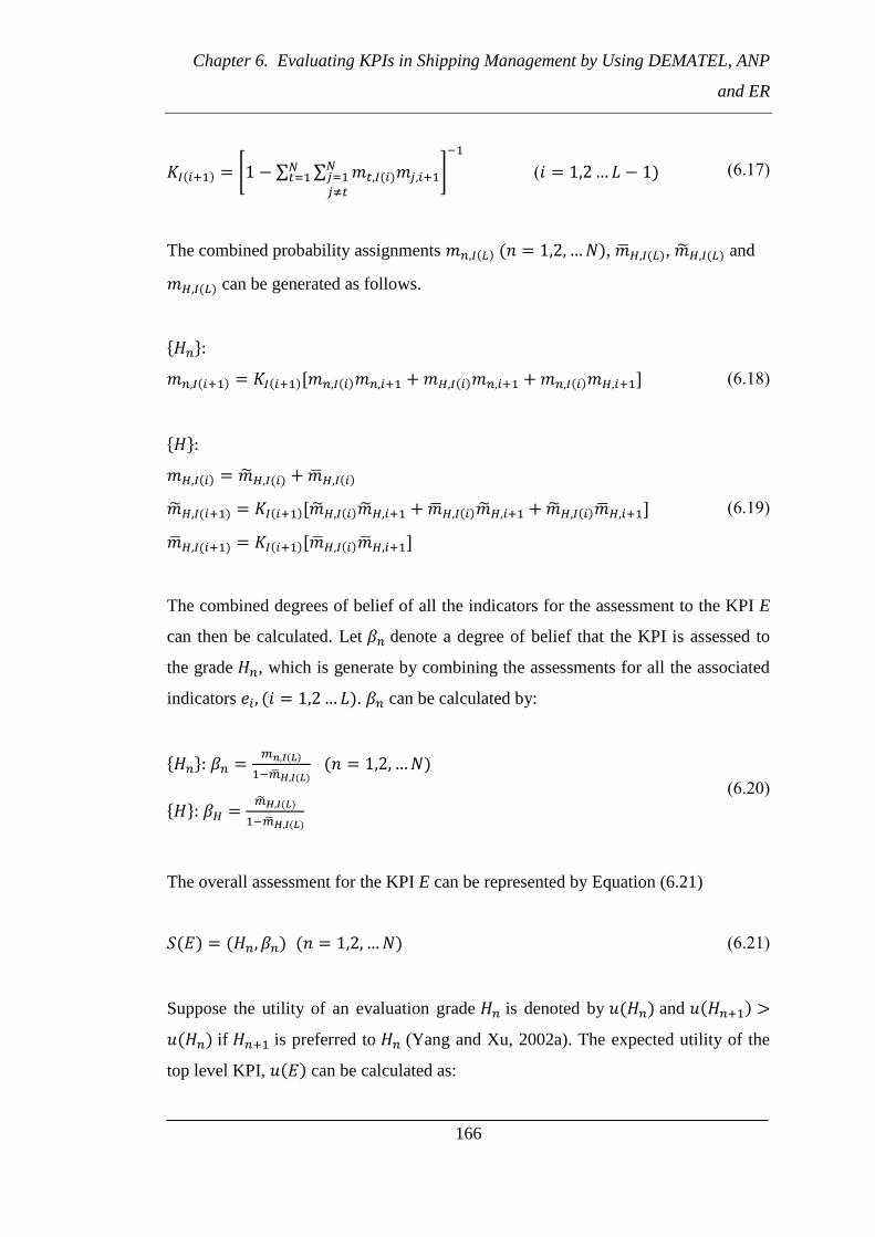
Chapter 6. Evaluating KPIs in Shipping Management by Using DEMATEL, ANP
and ER
166
𝐾𝐼 𝑖+ [1 − ∑ ∑ 𝑚𝑡 𝐼 𝑖 𝑚𝑗 𝑖+ 𝑁𝑗= 𝑗≠𝑡
𝑁𝑡= ]
−
(𝑖 1 2 𝐿 − 1 (6.17)
The combined probability assignments 𝑚𝑛 𝐼 𝐿 𝑛 1 2 𝑁 , �̅�𝐻 𝐼 𝐿 , �̃�𝐻 𝐼 𝐿 and
𝑚𝐻 𝐼 𝐿 can be generated as follows.
{𝐻𝑛}:
𝑚𝑛 𝐼 𝑖+ 𝐾𝐼 𝑖+ [𝑚𝑛 𝐼 𝑖 𝑚𝑛 𝑖+ + 𝑚𝐻 𝐼 𝑖 𝑚𝑛 𝑖+ + 𝑚𝑛 𝐼 𝑖 𝑚𝐻 𝑖+ ] (6.18)
{𝐻}:
𝑚𝐻 𝐼 𝑖 �̃�𝐻 𝐼 𝑖 + �̅�𝐻 𝐼 𝑖
�̃�𝐻 𝐼 𝑖+ 𝐾𝐼 𝑖+ [�̃�𝐻 𝐼 𝑖 �̃�𝐻 𝑖+ + �̅�𝐻 𝐼 𝑖 �̃�𝐻 𝑖+ + �̃�𝐻 𝐼 𝑖 �̅�𝐻 𝑖+ ]
�̅�𝐻 𝐼 𝑖+ 𝐾𝐼 𝑖+ [�̅�𝐻 𝐼 𝑖 �̅�𝐻 𝑖+ ]
(6.19)
The combined degrees of belief of all the indicators for the assessment to the KPI E
can then be calculated. Let 𝛽𝑛 denote a degree of belief that the KPI is assessed to
the grade 𝐻𝑛, which is generate by combining the assessments for all the associated
indicators 𝑒𝑖 𝑖 1 2 𝐿 . 𝛽𝑛 can be calculated by:
{𝐻𝑛}: 𝛽𝑛 𝑚𝑛 𝐼 𝐿
−�̅�𝐻 𝐼 𝐿 𝑛 1 2 𝑁
{𝐻}: 𝛽𝐻 �̃�𝐻 𝐼 𝐿
−�̅�𝐻 𝐼 𝐿
(6.20)
The overall assessment for the KPI E can be represented by Equation (6.21)
𝑆 𝐸 𝐻𝑛 𝛽𝑛 𝑛 1 2 𝑁 (6.21)
Suppose the utility of an evaluation grade 𝐻𝑛 is denoted by 𝑢 𝐻𝑛 and 𝑢 𝐻𝑛+ >
𝑢 𝐻𝑛 if 𝐻𝑛+ is preferred to 𝐻𝑛 (Yang and Xu, 2002a). The expected utility of the
top level KPI, 𝑢 𝐸 can be calculated as:

Chapter 6. Evaluating KPIs in Shipping Management by Using DEMATEL, ANP
and ER
167
𝑢 𝐸 ∑ 𝛽𝑛𝑢 𝐻𝑛 𝑁𝑛= (6.22)
The utility value of each linguistic term 𝑢 𝐻𝑛 is obtained in a linear manner
through using Equation (6.23).
𝑢 𝐻𝑛 𝑉𝑛−𝑉𝑚𝑖𝑛
𝑉𝑚𝑎𝑥−𝑉𝑚𝑖𝑛 (6.23)
where 𝑉𝑚𝑎𝑥 is the ranking value of the most preferred linguistic term, 𝑉𝑚𝑖𝑛 is the
ranking value of the least preferred linguistic term and 𝑉𝑛 is the ranking value of the
linguistic term considered.
When several parent level KPIs need to be compared, the above process can be
repeated to obtain the estimates for those parent level performance indicators. Once
the utility values for the top level KPIs are calculated, they can then be benchmarked.
𝐸𝑙 is said to be preferred to 𝐸𝑘 if 𝑢 𝐸𝑙 > 𝑢 𝐸𝑘 .
The whole process of ER calculation can be performed by using an ER calculation
software package which is called Intelligent Decision System via Evidential
Reasoning, or IDS (Yang and Xu, 2002b).
6.4 A Case Study of KPI Tree Management in a Shipping
Management Company
A world leading shipping management company established a performance
monitoring programme by using KPIs in order to monitor and measure its current
performance, and to compare performances between different function areas and
different periods of time. The indicators that are important to the company objective
are identified. Table 6.1 displays the pre-established KPI tree structure containing
all the indicators at the KPIs (upper) and PIs (lower) levels.

Chapter 6. Evaluating KPIs in Shipping Management by Using DEMATEL, ANP
and ER
168
Table 6.1 KPI tree structure Objective KPI PI
Co
mp
an
y o
ver
all
per
form
an
ce
(A) Health and Safety
Management & Performance
A1) Lost time injury rate
A2) Total recordable case frequency
A3) Near miss reports received
(B) Quality Assurance
B1) Overdue NCNs
B2) Overdue NCNs longer than 1 month
B3) Overdue audits - office
B4) Overdue SHEQ audits - ships
(C) Environmental
Performance
C1) Contained spillage
C2) Pollution incidents
C3) Port authority environmental violations
C4) Suppliers with ISO 14001 accreditation
(D) HR Management
Performance
D1) Crew retention
D2) Office staff retention
(E) Operational Performance
E1) Unscheduled downtime. Out of service - offshore
E2) Unscheduled downtime. Out of service - marine
E3) Overdue vessel technical inspections
E4) Port state detentions
(F) Technical Performance F1) Outstanding PM items
(G) Purchasing & Accounting
Performance
G1) Outstanding invoices not approved for payment
(NAPS)
G2) Purchasing feedback reports
6.4.1 Assess the Interdependencies of the KPIs Using DEMATEL
A questionnaire was designed for the evaluation of influencing levels among all
KPIs. The questionnaire contains seven comparison tables. Each comparison table
requires the appraiser to provide the judgement of the degree of influence of each
KPI listed in the column to the target KPI list on the top row of the table. Table 6.2 is
a table from the questionnaire to investigate the degree of influences that all other
KPIs have in regards to the target KPI (A) Health and Safety Management &
Performance. The same questionnaire tables are designed for the rest of KPIs. The
detailed questionnaire can be found in Appendix 4.

Chapter 6. Evaluating KPIs in Shipping Management by Using DEMATEL, ANP
and ER
169
Table 6.2 Evaluation table for the degree of influences
Degree of influence that each of the following KPI directly has on the target KPI:
(A)Health and Safety Management & Performance
KPI
Degree of influence
0: No influence, 1:Low influence
2:Medium influence: 3: High influence
4:Very high influence
0 1 2 3 4
(B) Quality Assurance
(C) Environmental Performance
(D) HR Management Performance
(E) Operational Performance
(F) Technical Performance
(G) Purchasing & Accounting
Performance
Data is gathered through the responses of the questionnaires for the DEMATEL
study.
Step 1: Compute the average matrix (M)
The matrix 𝑀 [𝑚𝑖𝑗] is constructed based on the data collected as below:
𝑀 [𝑚𝑖𝑗]
[ 0 2 2 2 4 2 12 0 4 3 4 3 32 3 0 2 2 4 11 2 0 0 1 2 22 4 3 0 0 2 12 3 3 1 2 0 11 3 1 1 1 1 0]
Step 2: Normalize the average matrix (M) and obtain the normalized direct relation
matrix (D)
𝑆 𝑀𝑖𝑛 [
𝑚𝑎𝑥1≤𝑖≤𝑛 ∑ 𝑚𝑖𝑗𝑛𝑗=1
𝑚𝑎𝑥1≤𝑖≤𝑛 ∑ 𝑚𝑖𝑗𝑛𝑖=1
] 𝑀𝑖𝑛 [
7
9] 0.0526

Chapter 6. Evaluating KPIs in Shipping Management by Using DEMATEL, ANP
and ER
170
The relation matrix (D) can then be calculated by using Equation (6.1).
𝐷 𝑀 × 𝑆
[ 0 2 2 2 4 2 12 0 4 3 4 3 32 3 0 2 2 4 11 2 0 0 1 2 22 4 3 0 0 2 12 3 3 1 2 0 11 3 1 1 1 1 0]
× 0.0526
[
0 0.105 0.105 0.105 0.211 0.105 0.0530.105 0 0.211 0.158 0.211 0.158 0.1580.105 0.158 0 0.105 0.105 0.211 0.0530.053 0.105 0 0 0.053 0.105 0.1050.105 0.211 0.158 0 0 0.105 0.0530.105 0.158 0.158 0.053 0.105 0 0.0530.053 0.158 0.053 0.053 0.053 0.053 0 ]
Step 3: Calculate the total relation matrix (T)
The total relation matrix T is obtained by following Equation (6.2).
𝑇 𝐷 𝐼 − 𝐷 −
[ 0.178 0.377 0.333 0.247 0.421 0.335 0.2050.337 0.386 0.499 0.35 0.501 0.467 0.3510.289 0.438 0.26 0.267 0.358 0.442 0.2210.158 0.267 0.152 0.098 0.199 0.238 0.1970.278 0.46 0.389 0.172 0.253 0.345 0.210.268 0.407 0.373 0.208 0.334 0.239 0.2030.168 0.321 0.211 0.16 0.214 0.211 0.11 ]
Step 4: Calculate the sums of rows and columns of the total relation matrix (T)
The degree of importance for each KPI is calculated through Equations (6.3) and
(6.4) and is shown in Table 6.3.

Chapter 6. Evaluating KPIs in Shipping Management by Using DEMATEL, ANP
and ER
171
Table 6.3 Degree of importance through DEMATEL
r + c r - c
A 3.773 0.42
B 5.545 0.236
C 4.492 0.057
D 2.808 -0.19
E 4.387 -0.17
F 4.308 -0.24
G 2.89 -0.1
With the highest 𝑟𝑖 + 𝑐𝑗 value, KPI B plays higher importance than the others in
the whole KPI system where KPI D is least important with the lowest 𝑟𝑖 + 𝑐𝑗
value. KPI A, B and C are act as net causes ( 𝑟𝑖 − 𝑐𝑗 >0), while KPI D, E, F and G
are net receivers (𝑟𝑖 − 𝑐𝑗) < 0 .
Step 5: Set threshold value (α) and obtain the impact relations-map (IRM).
By using Equation (6.5), the threshold value is obtained as 𝛼 0.28778. The values
below 𝛼 are set to zero and the total relation matrix 𝑇 with 𝛼 cut is changed to matrix
𝑇𝛼 and is shown as below:
𝑇𝛼
[
0 0.377 0.333 0 0.421 0.335 00.337 0.386 0.499 0.35 0.501 0.467 0.3510.289 0.438 0 0 0.358 0.442 0
0 0 0 0 0 0 00 0.46 0.389 0 0 0.345 00 0.407 0.373 0 0.334 0 00 0.321 0 0 0 0 0 ]
The IRM is derived from DEMATEL and is shown in Figure 6.4.

Chapter 6. Evaluating KPIs in Shipping Management by Using DEMATEL, ANP
and ER
172
Figure 6.4 impact relations-map from DEMATEL
6.4.2 Obtain the Weights for the Lower Level Indicators by using the ANP
method
Through experts’ judgements, the existence of interdependency among the lower
level indicators is identified based on the results from DEMATEL. This activity
clarifies the interdependency between lower level indicators which can also adjust
the interdependency relationship among KPIs. By doing this, the number of pairwise
comparisons that need to be carried out is significantly reduced. In our case, without
the experts’ judgement, pairwise comparisons need to be conducted for all the lower
level indicators whose upper level KPIs were identified as interdependent through
DEMATEL analysis. The number of such comparisons is 360. However, experts
have filtered those lower level indicators down to the ones that actually affect each
other and the pairwise comparisons need only to be conducted among them. This
activity has reduced the number of pairwise comparison to 60.
To obtain the local weights, questionnaires with pairwise comparison matrices for
𝑟𝑖 + 𝑐𝑗 (Degree of importance)
importance)
𝑟𝑖 − 𝑐𝑗
A
(3.77, 0.42)
B (5.55, 0.24)
C (4.49, 0.06)
D (2.81, -0.19)
E (4.39, -0.17) F
(4.31, -0.24)
G
(2.89, -0.1)
Net receiver Net cause

Chapter 6. Evaluating KPIs in Shipping Management by Using DEMATEL, ANP
and ER
173
indicators with interdependency relationships are created. Table 6.4 is a pairwise
comparison table for the evaluation of influences among PIs in regards to PI (A2).
Similar comparison matrices are established for all the KPIs and PIs that have been
identified with interdependency. The detailed questionnaire is attached in Appendix
5 and Appendix 6.
The evaluations obtained are used to calculate the priority vector of an indicator
through Equation (6.7). For example, the evaluations given for the pairwise
comparison matrix in Table 6.4 are presented in Table 6.5.
Table 6.4 Pairwise comparison table for the evaluation of influences
Which indicator in the pair (on the same row) influences A2) Total Recordable
Case Frequency more with respect to the (A) Health and Safety Management &
Performance, and how much more than the other indicator
No.
PI
(Extreme Influence: 9、Substantial Influence: 7、
Essential or Strong Influence: 5、
Moderate Influence: 3、Equal Influence: 1)
PI
1 (C1)Contained
Spillage ( ) 9 8 7 6 5 4 3 2 1 2 3 4 5 6 7 8 9 (C2)Pollution
Incidents ( )
2
(C1)Contained
Spillage ( ) 9 8 7 6 5 4 3 2 1 2 3 4 5 6 7 8 9 (C3)Port Authority
Environmental
Violations ( )
3
(C2)Pollution
Incidents ( ) 9 8 7 6 5 4 3 2 1 2 3 4 5 6 7 8 9 (C3)Port Authority
Environmental
Violations ( )
Table 6.5 Evaluations for the level of influences among C1, C2 and C3 in regards to
indicator A1
A1 C1 C2 C3 Priorities
C1 1 5 5 0.7143
C2 0.2 1 1 0.1429
C3 0.2 1 1 0.1429

Chapter 6. Evaluating KPIs in Shipping Management by Using DEMATEL, ANP
and ER
174
The priority vector for C1 is calculated as below:
𝑤𝑐 1
𝑚∑
𝑎𝑘𝑗
∑ 𝑎𝑖𝑗𝑛𝑖=
𝑚
𝑗=
1
3(
1
1 + 0.2 + 0.2+
5
1 + 1 + 5+
5
1 + 1 + 5) 0.7143
The priority vectors for C2 and C3 in regards to A1 are obtained in the same way
and listed in Table 6.5. The unweighted supermatrix (Table 6.6) is constructed by
using the priority vectors for all the indicators, where “0” is given when there is no
interaction between any two indicators. The cluster weight matrix (Table 6.7) is
generated containing the priority vectors for all the KPIs, which are obtained by
using the same method. To build the weighted supermatrix (Table 6.8), priority
vectors in the unweighted supermatrix are multiplied by the priority vectors of the
corresponding clusters. For example, the priority vector for KPI C in regards to KPI
A is 1. Each priority vector for PIs under KPI C in regards to PIs under KPI A is to
be multiplied by 1. Therefore, all priority vectors in Table 6.5 are multiplied by 1 to
achieve the values in the weighted supermatrix. The supermatrix is then converged to
a limiting supermatrix (Table 6.9) and the global weights for all the lower level
indicators are listed in Table 6.10.
The calculation process can be performed by the computer software –
“SuperDecisions”. “SuperDecisons” is decision making software based on the AHP
and ANP. It is a simple easy-to-use package for constructing decision models with
dependence and feedback and computing results using the supermatrices of the ANP
(Adams and Saaty, 2003). Figure 6.5 is the relation map produced by the software.

Chapter 6. Evaluating KPIs in Shipping Management by Using DEMATEL, ANP
and ER
175
Figure 6.5 Relationship diagram created in “Super decisions” software

Chapter 6. Evaluating KPIs in Shipping Management by Using DEMATEL, ANP and ER
176
Table 6.6 Unweighted supermatrix
A1 A2 A3 B1 B2 B3 B4 C1 C2 C3 C4 D1 D2 E1 E2 E3 E4 F1 G1 G2 Objective
A1 0.0000 0.0000 0.0000 0.0000 0.0000 0.0000 0.0000 0.0000 0.0000 0.2897 0.0000 0.0000 0.0000 0.0000 0.0000 0.0000 0.8000 0.0000 0.0000 0.0000 0.0660
A2 0.0000 0.0000 0.0000 0.0000 0.0000 0.0000 0.0000 0.0000 0.0000 0.6554 0.0000 0.0000 0.0000 0.0000 0.0000 0.0000 0.2000 0.0000 0.0000 0.0000 0.3187
A3 0.0000 0.0000 0.0000 0.0000 0.0000 0.0000 0.0000 0.0000 0.0000 0.0549 0.0000 0.0000 0.0000 0.0000 0.0000 0.0000 0.0000 0.0000 0.0000 0.0000 0.6153
B1 0.0000 0.0000 0.0000 0.0000 0.1250 0.0000 0.0000 0.0626 0.1265 0.1095 0.0000 0.3333 0.0000 0.0000 0.0000 0.2493 0.0000 0.0836 0.0000 0.0000 0.2190
B2 0.0000 0.0000 0.0000 0.8571 0.0000 0.0000 0.0000 0.4791 0.1865 0.3090 0.0000 0.3333 0.0000 0.0000 0.0000 0.5936 0.0000 0.4443 0.0000 0.0000 0.0502
B3 0.0000 0.0000 0.0000 0.0000 0.0000 0.0000 0.0000 0.0000 0.0000 0.0000 0.0000 0.0000 0.0000 0.0000 0.0000 0.0000 0.0000 0.0000 0.0000 0.0000 0.2190
B4 0.0000 0.0000 0.0000 0.1429 0.8750 0.0000 0.0000 0.4583 0.6870 0.5816 0.0000 0.3333 0.0000 0.0000 0.0000 0.1571 0.0000 0.4721 0.0000 0.0000 0.5119
C1 0.0000 0.7143 0.0000 0.0000 0.0000 0.0000 0.0000 0.0000 0.0000 0.0000 0.0000 0.0000 0.0000 0.0556 0.0540 0.1939 0.1158 0.1991 0.0000 0.0000 0.1028
C2 0.0000 0.1429 0.0000 0.0000 0.0000 0.0000 0.0000 0.0000 0.0000 0.0000 0.0000 0.0000 0.0000 0.4815 0.5891 0.7429 0.4417 0.0675 0.0000 0.0000 0.5881
C3 0.0000 0.1429 0.0000 0.0000 0.0000 0.0000 0.0000 0.0000 0.0000 0.0000 0.0000 0.0000 0.0000 0.4629 0.3568 0.0633 0.4057 0.7334 0.0000 0.0000 0.2578
C4 0.0000 0.0000 0.0000 0.0000 0.0000 0.0000 0.0000 0.0000 0.0000 0.0000 0.0000 0.0000 0.0000 0.0000 0.0000 0.0000 0.0368 0.0000 0.0000 0.0000 0.0512
D1 0.0000 0.0000 0.0000 0.0000 0.0000 0.0000 0.0000 0.0000 0.0000 0.0000 0.0000 0.0000 0.0000 0.0000 0.0000 0.0000 0.0000 0.0000 0.0000 0.0000 0.5000
D2 0.0000 0.0000 0.0000 0.0000 0.0000 0.0000 0.0000 0.0000 0.0000 0.0000 0.0000 0.0000 0.0000 0.0000 0.0000 0.0000 0.0000 0.0000 0.0000 0.0000 0.5000
E1 0.0000 0.0000 0.0000 0.0000 0.0000 0.0000 0.0000 0.0000 0.0000 0.0000 0.0000 0.0000 0.0000 0.0000 0.0000 0.0000 0.0000 0.1000 0.0000 0.0000 0.1581
E2 0.0000 0.0000 0.0000 0.0000 0.0000 0.0000 0.0000 0.0000 0.0000 0.0000 0.0000 0.0000 0.0000 0.0000 0.0000 0.0000 0.0000 0.1000 0.0000 0.0000 0.1680
E3 0.0000 0.0000 0.0000 0.1250 0.0000 0.0000 0.0000 0.0000 0.1111 0.0000 0.0000 0.0000 0.0000 0.0000 0.0000 0.0000 0.0000 0.0000 0.0000 0.0000 0.0411
E4 0.0000 0.0000 0.0000 0.8750 0.0000 0.0000 0.0000 0.0000 0.8889 0.0000 0.0000 0.0000 0.0000 0.0000 0.0000 0.0000 0.0000 0.8000 0.0000 0.0000 0.6327
F1 0.0000 0.0000 0.0000 1.0000 1.0000 0.0000 0.0000 0.0000 0.0000 0.0000 0.0000 0.0000 0.0000 0.0000 0.0000 1.0000 0.0000 0.0000 0.0000 0.0000 1.0000
G1 0.0000 0.0000 0.0000 0.0000 0.0000 0.0000 0.0000 0.0000 0.0000 0.0000 0.0000 0.0000 0.0000 0.0000 0.0000 0.0000 0.0000 0.0000 0.0000 0.0000 0.8750
G2 0.0000 0.0000 0.0000 0.0000 0.0000 0.0000 0.0000 0.0000 0.0000 0.0000 0.0000 0.0000 0.0000 0.0000 0.0000 0.0000 0.0000 0.0000 0.0000 0.0000 0.1250
Objective 0.0000 0.0000 0.0000 0.0000 0.0000 0.0000 0.0000 0.0000 0.0000 0.0000 0.0000 0.0000 0.0000 0.0000 0.0000 0.0000 0.0000 0.0000 0.0000 0.0000 0.0000

Chapter 6. Evaluating KPIs in Shipping Management by Using DEMATEL, ANP and ER
177
Table 6.7 Cluster weight matrix
A B C D E F G Objective
A 0.0000 0.0000 0.7891 0.0000 0.7890 0.0000 0.0000 0.5389
B 0.0000 0.6885 0.1031 1.0000 0.1031 0.7641 0.0000 0.2298
C 1.0000 0.0000 0.0000 0.0000 0.1078 0.1210 0.0000 0.0685
D 0.0000 0.0000 0.0000 0.0000 0.0000 0.0000 0.0000 0.0363
E 0.0000 0.1148 0.1078 0.0000 0.0000 0.1149 0.0000 0.0521
F 0.0000 0.1967 0.0000 0.0000 0.0001 0.0000 0.0000 0.0327
G 0.0000 0.0000 0.0000 0.0000 0.0000 0.0000 0.0000 0.0416
Objective 0.0000 0.0000 0.0000 0.0000 0.0000 0.0000 0.0000 0.0000

Chapter 6. Evaluating KPIs in Shipping Management by Using DEMATEL, ANP and ER
178
Table 6.8 Weighted supermatrix
A1 A2 A3 B1 B2 B3 B4 C1 C2 C3 C4 D1 D2 E1 E2 E3 E4 F1 G1 G2 Objective
A1 0.0000 0.0000 0.0000 0.0000 0.0000 0.0000 0.0000 0.0000 0.0000 0.2563 0.0000 0.0000 0.0000 0.0000 0.0000 0.0000 0.7038 0.0000 0.0000 0.0000 0.0356
A2 0.0000 0.0000 0.0000 0.0000 0.0000 0.0000 0.0000 0.0000 0.0000 0.5796 0.0000 0.0000 0.0000 0.0000 0.0000 0.0000 0.1760 0.0000 0.0000 0.0000 0.1717
A3 0.0000 0.0000 0.0000 0.0000 0.0000 0.0000 0.0000 0.0000 0.0000 0.0486 0.0000 0.0000 0.0000 0.0000 0.0000 0.0000 0.0000 0.0000 0.0000 0.0000 0.3316
B1 0.0000 0.0000 0.0000 0.0000 0.0972 0.0000 0.0000 0.0626 0.0619 0.0127 0.0000 0.3333 0.0000 0.0000 0.0000 0.1218 0.0000 0.0639 0.0000 0.0000 0.0503
B2 0.0000 0.0000 0.0000 0.5902 0.0000 0.0000 0.0000 0.4791 0.0912 0.0357 0.0000 0.3333 0.0000 0.0000 0.0000 0.2901 0.0000 0.3395 0.0000 0.0000 0.0115
B3 0.0000 0.0000 0.0000 0.0000 0.0000 0.0000 0.0000 0.0000 0.0000 0.0000 0.0000 0.0000 0.0000 0.0000 0.0000 0.0000 0.0000 0.0000 0.0000 0.0000 0.0503
B4 0.0000 0.0000 0.0000 0.0984 0.6806 0.0000 0.0000 0.4583 0.3358 0.0672 0.0000 0.3333 0.0000 0.0000 0.0000 0.0767 0.0000 0.3607 0.0000 0.0000 0.1176
C1 0.0000 0.7143 0.0000 0.0000 0.0000 0.0000 0.0000 0.0000 0.0000 0.0000 0.0000 0.0000 0.0000 0.0556 0.0540 0.0991 0.0139 0.0241 0.0000 0.0000 0.0070
C2 0.0000 0.1429 0.0000 0.0000 0.0000 0.0000 0.0000 0.0000 0.0000 0.0000 0.0000 0.0000 0.0000 0.4815 0.5891 0.3795 0.0531 0.0082 0.0000 0.0000 0.0403
C3 0.0000 0.1429 0.0000 0.0000 0.0000 0.0000 0.0000 0.0000 0.0000 0.0000 0.0000 0.0000 0.0000 0.4629 0.3568 0.0323 0.0488 0.0887 0.0000 0.0000 0.0177
C4 0.0000 0.0000 0.0000 0.0000 0.0000 0.0000 0.0000 0.0000 0.0000 0.0000 0.0000 0.0000 0.0000 0.0000 0.0000 0.0000 0.0044 0.0000 0.0000 0.0000 0.0035
D1 0.0000 0.0000 0.0000 0.0000 0.0000 0.0000 0.0000 0.0000 0.0000 0.0000 0.0000 0.0000 0.0000 0.0000 0.0000 0.0000 0.0000 0.0000 0.0000 0.0000 0.0182
D2 0.0000 0.0000 0.0000 0.0000 0.0000 0.0000 0.0000 0.0000 0.0000 0.0000 0.0000 0.0000 0.0000 0.0000 0.0000 0.0000 0.0000 0.0000 0.0000 0.0000 0.0182
E1 0.0000 0.0000 0.0000 0.0000 0.0000 0.0000 0.0000 0.0000 0.0000 0.0000 0.0000 0.0000 0.0000 0.0000 0.0000 0.0000 0.0000 0.0115 0.0000 0.0000 0.0082
E2 0.0000 0.0000 0.0000 0.0000 0.0000 0.0000 0.0000 0.0000 0.0000 0.0000 0.0000 0.0000 0.0000 0.0000 0.0000 0.0000 0.0000 0.0115 0.0000 0.0000 0.0088
E3 0.0000 0.0000 0.0000 0.0143 0.0000 0.0000 0.0000 0.0000 0.0568 0.0000 0.0000 0.0000 0.0000 0.0000 0.0000 0.0000 0.0000 0.0000 0.0000 0.0000 0.0021
E4 0.0000 0.0000 0.0000 0.1004 0.0000 0.0000 0.0000 0.0000 0.4543 0.0000 0.0000 0.0000 0.0000 0.0000 0.0000 0.0000 0.0000 0.0919 0.0000 0.0000 0.0330
F1 0.0000 0.0000 0.0000 0.1967 0.2222 0.0000 0.0000 0.0000 0.0000 0.0000 0.0000 0.0000 0.0000 0.0000 0.0000 0.0005 0.0000 0.0000 0.0000 0.0000 0.0327
G1 0.0000 0.0000 0.0000 0.0000 0.0000 0.0000 0.0000 0.0000 0.0000 0.0000 0.0000 0.0000 0.0000 0.0000 0.0000 0.0000 0.0000 0.0000 0.0000 0.0000 0.0364
G2 0.0000 0.0000 0.0000 0.0000 0.0000 0.0000 0.0000 0.0000 0.0000 0.0000 0.0000 0.0000 0.0000 0.0000 0.0000 0.0000 0.0000 0.0000 0.0000 0.0000 0.0052
Objective 0.0000 0.0000 0.0000 0.0000 0.0000 0.0000 0.0000 0.0000 0.0000 0.0000 0.0000 0.0000 0.0000 0.0000 0.0000 0.0000 0.0000 0.0000 0.0000 0.0000 0.0000

Chapter 6. Evaluating KPIs in Shipping Management by Using DEMATEL, ANP and ER
179
Table 6.9 Limiting supermaterix
A1 A2 A3 B1 B2 B3 B4 C1 C2 C3 C4 D1 D2 E1 E2 E3 E4 F1 G1 G2 Objective
A1 0.0000 0.0724 0.0000 0.0724 0.0724 0.0000 0.0000 0.0724 0.0724 0.0724 0.0000 0.0724 0.0000 0.0724 0.0724 0.0724 0.0724 0.0724 0.0000 0.0000 0.0724
A2 0.0000 0.0497 0.0000 0.0497 0.0497 0.0000 0.0000 0.0497 0.0497 0.0497 0.0000 0.0497 0.0000 0.0497 0.0497 0.0497 0.0497 0.0497 0.0000 0.0000 0.0497
A3 0.0000 0.0030 0.0000 0.0030 0.0030 0.0000 0.0000 0.0030 0.0030 0.0030 0.0000 0.0030 0.0000 0.0030 0.0030 0.0030 0.0030 0.0030 0.0000 0.0000 0.0030
B1 0.0000 0.0543 0.0000 0.0543 0.0543 0.0000 0.0000 0.0543 0.0543 0.0543 0.0000 0.0543 0.0000 0.0543 0.0543 0.0543 0.0543 0.0543 0.0000 0.0000 0.0543
B2 0.0000 0.1812 0.0000 0.1812 0.1812 0.0000 0.0000 0.1812 0.1812 0.1812 0.0000 0.1812 0.0000 0.1812 0.1812 0.1812 0.1812 0.1812 0.0000 0.0000 0.1812
B3 0.0000 0.0000 0.0000 0.0000 0.0000 0.0000 0.0000 0.0000 0.0000 0.0000 0.0000 0.0000 0.0000 0.0000 0.0000 0.0000 0.0000 0.0000 0.0000 0.0000 0.0000
B4 0.0000 0.3667 0.0000 0.3667 0.3667 0.0000 0.0000 0.3667 0.3667 0.3667 0.0000 0.3667 0.0000 0.3667 0.3667 0.3667 0.3667 0.3667 0.0000 0.0000 0.3667
C1 0.0000 0.0698 0.0000 0.0698 0.0698 0.0000 0.0000 0.0698 0.0698 0.0698 0.0000 0.0698 0.0000 0.0698 0.0698 0.0698 0.0698 0.0698 0.0000 0.0000 0.0698
C2 0.0000 0.0246 0.0000 0.0246 0.0246 0.0000 0.0000 0.0246 0.0246 0.0246 0.0000 0.0246 0.0000 0.0246 0.0246 0.0246 0.0246 0.0246 0.0000 0.0000 0.0246
C3 0.0000 0.0342 0.0000 0.0342 0.0342 0.0000 0.0000 0.0342 0.0342 0.0342 0.0000 0.0342 0.0000 0.0342 0.0342 0.0342 0.0342 0.0342 0.0000 0.0000 0.0342
C4 0.0000 0.0004 0.0000 0.0004 0.0004 0.0000 0.0000 0.0004 0.0004 0.0004 0.0000 0.0004 0.0000 0.0004 0.0004 0.0004 0.0004 0.0004 0.0000 0.0000 0.0004
D1 0.0000 0.0000 0.0000 0.0000 0.0000 0.0000 0.0000 0.0000 0.0000 0.0000 0.0000 0.0000 0.0000 0.0000 0.0000 0.0000 0.0000 0.0000 0.0000 0.0000 0.0000
D2 0.0000 0.0000 0.0000 0.0000 0.0000 0.0000 0.0000 0.0000 0.0000 0.0000 0.0000 0.0000 0.0000 0.0000 0.0000 0.0000 0.0000 0.0000 0.0000 0.0000 0.0000
E1 0.0000 0.0019 0.0000 0.0019 0.0019 0.0000 0.0000 0.0019 0.0019 0.0019 0.0000 0.0019 0.0000 0.0019 0.0019 0.0019 0.0019 0.0019 0.0000 0.0000 0.0019
E2 0.0000 0.0019 0.0000 0.0019 0.0019 0.0000 0.0000 0.0019 0.0019 0.0019 0.0000 0.0019 0.0000 0.0019 0.0019 0.0019 0.0019 0.0019 0.0000 0.0000 0.0019
E3 0.0000 0.0039 0.0000 0.0039 0.0039 0.0000 0.0000 0.0039 0.0039 0.0039 0.0000 0.0039 0.0000 0.0039 0.0039 0.0039 0.0039 0.0039 0.0000 0.0000 0.0039
E4 0.0000 0.0449 0.0000 0.0449 0.0449 0.0000 0.0000 0.0449 0.0449 0.0449 0.0000 0.0449 0.0000 0.0449 0.0449 0.0449 0.0449 0.0449 0.0000 0.0000 0.0449
F1 0.0000 0.0914 0.0000 0.0914 0.0914 0.0000 0.0000 0.0914 0.0914 0.0914 0.0000 0.0914 0.0000 0.0914 0.0914 0.0914 0.0914 0.0914 0.0000 0.0000 0.0914
G1 0.0000 0.0000 0.0000 0.0000 0.0000 0.0000 0.0000 0.0000 0.0000 0.0000 0.0000 0.0000 0.0000 0.0000 0.0000 0.0000 0.0000 0.0000 0.0000 0.0000 0.0000
G2 0.0000 0.0000 0.0000 0.0000 0.0000 0.0000 0.0000 0.0000 0.0000 0.0000 0.0000 0.0000 0.0000 0.0000 0.0000 0.0000 0.0000 0.0000 0.0000 0.0000 0.0000
Objective 0.0000 0.0000 0.0000 0.0000 0.0000 0.0000 0.0000 0.0000 0.0000 0.0000 0.0000 0.0000 0.0000 0.0000 0.0000 0.0000 0.0000 0.0000 0.0000 0.0000 0.0000
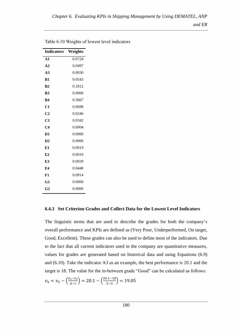
Chapter 6. Evaluating KPIs in Shipping Management by Using DEMATEL, ANP
and ER
180
Table 6.10 Weights of lowest level indicators
6.4.3 Set Criterion Grades and Collect Data for the Lowest Level Indicators
The linguistic terms that are used to describe the grades for both the company’s
overall performance and KPIs are defined as (Very Poor, Underperformed, On target,
Good, Excellent). These grades can also be used to define most of the indicators. Due
to the fact that all current indicators used in the company are quantitative measures,
values for grades are generated based on historical data and using Equations (6.9)
and (6.10). Take the indicator A3 as an example, the best performance is 20.1 and the
target is 18. The value for the in-between grade “Good” can be calculated as follows:
𝑣4 𝑣5 − (𝑣5−𝑣3
ℎ−𝑙) 20.1 − (
0. − 8
5−3) 19.05
Indicators Weights
A1 0.0724
A2 0.0497
A3 0.0030
B1 0.0543
B2 0.1812
B3 0.0000
B4 0.3667
C1 0.0698
C2 0.0246
C3 0.0342
C4 0.0004
D1 0.0000
D2 0.0000
E1 0.0019
E2 0.0019
E3 0.0039
E4 0.0448
F1 0.0914
G1 0.0000
G2 0.0000

Chapter 6. Evaluating KPIs in Shipping Management by Using DEMATEL, ANP
and ER
181
The in-between grade “under performed” is calculated by using the value of worst
performance 12 and the target value 18.
𝑣 𝑣 + (𝑣3−𝑣1
ℎ−𝑙) 18 − (
8−
3− ) 15
Indicators that are assessed by either “0 value” or “over 0”, such as B3 and B4, are
defined by the grades “>0” and “0”. These grades are transformed into the grades
defining the upper level KPIs by using the fuzzy rule base belief structure. Take B3
as an example, the fuzzy rule base belief structure can be constructed as:
R1: IF “Overdue Audits – Office” is “0”, then “Quality Assurance” is “Excellent”.
R2: If ““Overdue Audits – Office” is “>0”, then “Quality Assurance” is “Very
poor”.
In a similar way, the scores for the other grades are obtained and listed in Table 6.11.
6.4.4 Transform the Evaluation and Synthesis Indicators from the Lowest
Level to Top Level by using an ER Algorithm
The evaluations are obtained for all indicators, which are then transformed into the
associated linguistic terms with belief degrees based on the scores of the evaluation
grades in Table 6.11. Take the evaluation associated with indicator A1 in month 2 as
an example. The value was given as 0.39 per 1,000,000 man hours. By using
Equation (6.12), the value can be transformed and presented as the associated belief
degrees of the evaluation grades as follows:
𝛽4 𝐴 𝑣𝑔 𝐴1−𝑣5 𝐴1
𝑣4 𝐴1−𝑣5 𝐴1
0.39−0.
0.475−0. 0.691
𝛽5 𝐴 1 − 𝛽4 𝐴 0.309

Chapter 6. Evaluating KPIs in Shipping Management by Using DEMATEL, ANP
and ER
182
Table 6.11 Indicator evaluations and grades associated with linguistic terms
KPI PI Units
Very
Poor
Underper
formed
On
Target Good
Excelle
nt
(A) Health and Safety
Management
& Performance
A1) Lost time injury rate
Per 1,000,000 man hrs
1.3 1.025 0.75 0.475 0.2
A2) Total recordable case frequency
Per 1,000,000 man hrs
3.6 2.75 1.9 1.05 0.2
A3) Near miss reports received
Av. No. / Vsl / month
12 15 18 19.05 20.1
(B) Quality
Assurance
B1) Overdue NCNs Number of NCNs
15 14 13 12.5 12
B2) Overdue NCNs longer than 1 month OD > 1 mth
16 14.5 13 11.5 10
B3) Overdue audits - office Number
>0 0
B4) Overdue SHEQ audits - ships Number
>0 0
(C) Environment
al
Performance
C1) Contained spillage No. / year
8 5.5 3 2 1
C2) Pollution
incidents Number >0
0
C3) Port authority environmental
violations Number >0
0
C4) Suppliers with ISO 14001
accreditation
% on supplier list
0.14 0.145 0.15 0.155 0.16
(D) HR Management
Performance
D1) Crew retention % retention 85.13 88.565 92 95.435 98.87
D2) Office staff retention % retention
96 97 98 99 100
(E) Operational Performance
E1) Unscheduled downtime. Out of service - offshore
% days per year
0.0673 0.05115 0.035 0.01885 0.0027
E2) Unscheduled
downtime. Out of service - marine
% days per year
0.0666 0.0508 0.035 0.0192 0.0034
E3) Overdue Vsl
technical inspections Number
>0
0
E4) Port state detentions No. / vessel
>0
0
(F) Technical
Performance F1) Outstanding
PM items
% outstanding
0.03 0.025 0.02 0.015 0.01
(G)
Purchasing & Accounting
Performance
G1) Outstanding invoices not approved for
payment (NAPS) No. / month 581 490.5 400 309.5 219
G2) Purchasing feedback reports No. / month
4 7 10 11 12

Chapter 6. Evaluating KPIs in Shipping Management by Using DEMATEL, ANP
and ER
183
The results from the evaluation of A1 can then be expressed as (0% Very poor, 0%
Underperformed, 0% On target, 69.1% Good, 30.9% Excellent). Similarly, all the
evaluations are transformed and listed in Table 6.12.
The results are synthesised by following Equations (6.13) to (6.21). Take A1 and A2
in month 2 as examples. The weights for A1 and A2 were obtained in section 6.4.2,
which are 0.0724 and 0.0497, respectively. To synthesise the two indicators, their
weights are normalized to the unit 1. The normalized weights are: 𝑤𝐴 0.593 and
𝑤𝐴 0.407. The two indicators can then be synthesised as below.
1) Obtain probability mass by using Equation (6.13)
𝑚 𝑤 𝛽 0.593 × 0 0
𝑚 𝑤 𝛽 0.593 × 0 0
𝑚3 𝑤 𝛽3 0.593 × 0 0
𝑚4 𝑤 𝛽4 0.593 × 0.691 0.409
𝑚5 𝑤 𝛽5 0.593 × 0.309 0.184
𝑚 𝑤 𝛽 0.407 × 0 0
𝑚 𝑤 𝛽 0.407 × 0 0
𝑚3 𝑤 𝛽3 0.407 × 0 0
𝑚4 𝑤 𝛽4 0.407 × 0.288 0.117
𝑚5 𝑤 𝛽5 0.407 × 0.712 0.29
2) Calculate the remaining probability mass by using Equation (6.15) and (6.16).
�̅�𝐻 1 − 𝑤 1 − 0.593 0.407
�̃�𝐻 𝑤 (1 − ∑ 𝛽𝑛 5𝑛= ) 0.593 1 − 1 0
𝑚𝐻 �̅�𝐻 + �̃�𝐻 0.407 + 0 0.407

Chapter 6. Evaluating KPIs in Shipping Management by Using DEMATEL, ANP
and ER
184
�̅�𝐻 1 − 𝑤 1 − 0.407 0.593
�̃�𝐻 𝑤 (1 − ∑ 𝛽𝑛 5𝑛= ) 0.407 1 − 1 0
𝑚𝐻 �̅�𝐻 + �̃�𝐻 0.593 + 0 0.593
3) Obtain the combined probability assignments by following Equations (6.17),
(6.18) and (6.19).
𝐾𝐼 𝑖+ [1 − ∑ ∑ 𝑚𝑡 𝐼 𝑖 𝑚𝑗 𝑖+ 𝑁𝑗= 𝑗≠𝑡
𝑁𝑡= ]
−
[1 − (𝑚 × 𝑚 + 𝑚 × 𝑚3 + 𝑚 × 𝑚4 + 𝑚 × 𝑚5 + 𝑚 ×
𝑚 + 𝑚 × 𝑚3 + 𝑚 × 𝑚4 + 𝑚 × 𝑚5 + 𝑚3 × 𝑚 + 𝑚3 ×
𝑚 + 𝑚3 × 𝑚4 + 𝑚3 × 𝑚5 + 𝑚4 × 𝑚 + 𝑚4 × 𝑚 + 𝑚4 ×
𝑚3 + 𝑚4 × 𝑚5 + 𝑚5 × 𝑚 + 𝑚5 × 𝑚 + 𝑚5 × 𝑚3 + 𝑚5 ×
𝑚4 )]−
[1 − 0.409 × 0.289 + 0.184 × 0.117 ]− 1.163
𝑚 𝐼 𝑖+ 𝐾𝐼 𝑖+ [𝑚 𝐼 𝑖 𝑚 𝑖+ + 𝑚𝐻 𝐼 𝑖 𝑚 𝑖+ + 𝑚 𝐼 𝑖 𝑚𝐻 𝑖+ ]
𝑚 𝐼 1.163[𝑚 × 𝑚 + 𝑚𝐻 × 𝑚 + 𝑚 × 𝑚𝐻 ]
1.163[0 × 0 + 0.407 × 0 + 0 × 0.593] 0
𝑚 𝐼 𝑖+ 𝐾𝐼 𝑖+ [𝑚 𝐼 𝑖 𝑚 𝑖+ + 𝑚𝐻 𝐼 𝑖 𝑚 𝑖+ + 𝑚 𝐼 𝑖 𝑚𝐻 𝑖+ ]
𝑚 𝐼 1.163[𝑚 × 𝑚 + 𝑚𝐻 × 𝑚 + 𝑚 × 𝑚𝐻 ]
1.163[0 × 0 + 0.407 × 0 + 0 × 0.593] 0
𝑚3 𝐼 𝑖+ 𝐾𝐼 𝑖+ [𝑚3 𝐼 𝑖 𝑚3 𝑖+ + 𝑚𝐻 𝐼 𝑖 𝑚3 𝑖+ + 𝑚3 𝐼 𝑖 𝑚𝐻 𝑖+ ]
𝑚3 𝐼 1.163[𝑚3 × 𝑚3 + 𝑚𝐻 × 𝑚3 + 𝑚3 × 𝑚𝐻 ]
1.163[0 × 0 + 0.407 × 0 + 0 × 0.593] 0

Chapter 6. Evaluating KPIs in Shipping Management by Using DEMATEL, ANP
and ER
185
𝑚4 𝐼 𝑖+ 𝐾𝐼 𝑖+ [𝑚4 𝐼 𝑖 𝑚4 𝑖+ + 𝑚𝐻 𝐼 𝑖 𝑚4 𝑖+ + 𝑚4 𝐼 𝑖 𝑚𝐻 𝑖+ ]
𝑚4 𝐼 1.163[𝑚4 × 𝑚4 + 𝑚𝐻 × 𝑚4 + 𝑚4 × 𝑚𝐻 ]
1.163[0.409 × 0.117 + 0.407 × 0.117 + 0.409 × 0.593] 0.394
𝑚5 𝐼 𝑖+ 𝐾𝐼 𝑖+ [𝑚5 𝐼 𝑖 𝑚5 𝑖+ + 𝑚𝐻 𝐼 𝑖 𝑚5 𝑖+ + 𝑚5 𝐼 𝑖 𝑚𝐻 𝑖+ ]
𝑚5 𝐼 1.163[𝑚5 × 𝑚5 + 𝑚𝐻 × 𝑚5 + 𝑚5 × 𝑚𝐻 ]
1.163[0.184 × 0.289 + 0.407 × 0.289 + 0.184 × 0.593] 0.325
�̃�𝐻 𝐼 𝑖+ 𝐾𝐼 𝑖+ [�̃�𝐻 𝐼 𝑖 �̃�𝐻 𝑖+ + �̅�𝐻 𝐼 𝑖 �̃�𝐻 𝑖+ + �̃�𝐻 𝐼 𝑖 �̅�𝐻 𝑖+ ]
�̃�𝐻 𝐼 1.163[ �̃�𝐻 �̃�𝐻 + �̅�𝐻 �̃�𝐻 + �̃�𝐻 �̅�𝐻 ]
1.163 0 × 0 + 0.407 × 0 + 0 × 0.593 0
�̅�𝐻 𝐼 𝑖+ 𝐾𝐼 𝑖+ [�̅�𝐻 𝐼 𝑖 �̅�𝐻 𝑖+ ]
�̅�𝐻 𝐼 𝐾𝐼 𝑖+ [�̅�𝐻 �̅�𝐻 ] 1.163 0.407 × 0.593 0.28
4) Calculate the combined degree of belief of the indicators through applying
Equation (6.20)
𝛽 𝑚1 𝐼 2
−�̅�𝐻 𝐼 2
0
−0. 8 0
𝛽 𝑚1 𝐼 2
−�̅�𝐻 𝐼 2
0
−0. 8 0
𝛽3 𝑚3 𝐼 2
−�̅�𝐻 𝐼 2
0
−0. 8 0
𝛽4 𝑚4 𝐼 2
−�̅�𝐻 𝐼 2
0.394
−0. 8 0.548
𝛽5 𝑚4 𝐼 2
−�̅�𝐻 𝐼 2
0.3 5
−0. 8 0.452
The overall assessment for A1 and A2 can then be expressed as (0% Very poor, 0%
underperformance, 0% on Target, 54.8% Good, 45.2% Excellent).

Chapter 6. Evaluating KPIs in Shipping Management by Using DEMATEL, ANP
and ER
186
5) Generate the utility value of the top level KPI by using Equations (6.22) and
(6.23).
Firstly, the utility values associated with each linguistic term are as below:
Very Poor Under Performance On Target Good Excellent
(1) (2) (3) (4) (5)
𝑢 𝐻 𝑉1−𝑉𝑚𝑖𝑛
𝑉𝑚𝑎𝑥−𝑉𝑚𝑖𝑛
−
5− 0
𝑢 𝐻 𝑉2−𝑉𝑚𝑖𝑛
𝑉𝑚𝑎𝑥−𝑉𝑚𝑖𝑛
−
5− 0.25
𝑢 𝐻3 𝑉3−𝑉𝑚𝑖𝑛
𝑉𝑚𝑎𝑥−𝑉𝑚𝑖𝑛
3−
5− 0.5
𝑢 𝐻4 𝑉4−𝑉𝑚𝑖𝑛
𝑉𝑚𝑎𝑥−𝑉𝑚𝑖𝑛
4−
5− 0.75
𝑢 𝐻5 𝑉5−𝑉𝑚𝑖𝑛
𝑉𝑚𝑎𝑥−𝑉𝑚𝑖𝑛
5−
5− 1
The utility value for the upper level KPI can then be calculated as follows.
𝑢 𝐸 ∑ 𝛽𝑛𝑢 𝐻𝑛 5𝑛= 0.548 × 0.75 + 0.452 × 1 0.863
In a similar way, all the indicators can be synthesised. This lengthy calculation can
be by performed in the Software IDS (Yang and Xu, 2002b).

Chapter 6. Evaluating KPIs in Shipping Management by Using DEMATEL, ANP
and ER
187
Figure 6.6 presents an outcome from IDS in regards to the company overall
performance over a four months period, where the utility value for each month are:
Month 1= 0.7991, Month 2 = 0.9690, Month 3 = 0.9594, and Month 4 = 0.9368.
Figure 6.6 Ranking for the company overall performance over four-month period
Similar comparisons can be conducted for various other purposes, such as, visualize
the comparison of KPIs for the given time frame (Figure 6.7)

Chapter 6. Evaluating KPIs in Shipping Management by Using DEMATEL, ANP
and ER
188
Figure 6.7 Comparison of KPIs over four-month period
6.5 Conclusion
As a performance measurement tool, KPIs have shown their great popularity in
practice. It helps identify existing issues, monitor performance and enable
performance comparison between different function areas. Like many other
industries, in shipping industry, the majority of current practitioners apply KPIs with
only quantitative data and without considering the importance of different indicators
or their interdependencies, which have restricted their applicability and caused biases
in results. This study developed a systematic method in KPI measurement to
overcome those issues and therefore, provided reliable and comparable results for
management to make rational decisions. In this research, DEMATEL and ANP were
used to obtain weights of indicators. The marriage of DEMATEL and ANP enabled
the calculation of weights for indicators by taking into consideration interdependency
among them. The use of the FER approach enabled the handling of both quantitative

Chapter 6. Evaluating KPIs in Shipping Management by Using DEMATEL, ANP
and ER
189
and qualitative data and synthesizing indicators on a KPI tree from the bottom to the
top level in a meaningful way.

Chapter 6. Evaluating KPIs in Shipping Management by Using DEMATEL, ANP and ER
190
Table 6.12 Belief degrees transformed from the evaluations form all indicators
KPI PI
Month 1 Month 2 Month 3 Month 4
Very
Poor
Under
Perfor
mance
On
Targ
et
Very
Good
Exce
llent
Very
Poor
Under
Perfor
mance
On
Targ
et
Very
Good
Exce
llent
Very
Poor
Unde
r
Perfo
rman
ce
On
Targ
et
Very
Good
Excel
lent
Very
Poor
Under
Perfor
mance
On
Targ
et
Very
Good
Excelle
nt
(A)
A1 0 0 0 0 1 0 0 0 0.691 0.309 0 0 0.418 0.582 0 0 0 0 0.509 0.491
A2 0 0 0 0 1 0 0 0 0.288 0.712 0 0 0 0.68 0.32 0 0 0 0.682 0.318
A3 0 1 0 0 0 0.733 0.267 0 0 0 0 0 0 0 1 1 0 0 0 0
(B)
B1 0 1 0 0 0 1 0 0 0 0 0 0 0 1 1 0 0 0 0
B2 0 0 0 0 1 0 0 0 0 1 0 0 0 0.667 0.333 0 0 0 0.667 0.333
B3 0 0 0 0 1 0 0 0 0 1 0 0 0 0 1 0 0 0 0 1
B4 1 0 0 0 0 0 0 0 0 1 0 0 0 0 1 0 0 0 0 1
(C)
C1 1 0 0 0 0 0 0 0 0 1 0 0 1 0 0 0 0 1 0 0
C2 0 0 0 0 1 0 0 0 0 1 0 0 0 0 1 0 0 0 0 1
C3 0 0 0 0 1 0 0 0 0 1 0 0 0 0 1 0 0 0 0 1
C4 0 0 0 0 1 0 0 0 0 1 0 0 0 0 1 1 0 0 0 0
(D)
D1 0 0 0 0 1 0 0 0 0.39 0.61 0 0 0 0.39 0.61 0 0 0 0.472 0.528
D2 0 0 0 0 1 0 0 1 0 0 0 0 0 0 1 0 0 0 0 1
(E)
E1 0 0 0 0 1 0 0 0 0 1 0 0 0 0.22 0.78 0 0 0 0.248 0.752
E2 0 0 0 0.11 0.89 0 0 0.64 0.32 0 0 0 0 0.468 0.532 0 0 0 0 1
E3 0 0 0 0 1 0 0 0 0 1 0 0 0 0 1 0 0 0 0 1
E4 0 0 0 0 1 0 0 0 0 1 0 0 0 0 1 0 0 0 0 1
(F) F1 0 0 1 0 0 0.6 0.4 0 0 0 1 0 0 0 0 0.2 0.8 0 0 0
(G) G1 1 0 0 0 0 0 0.729 0.27 0 0 0.702 0.298 0 0 0 0.315 0.685 0 0 0
G2 0 0 0 0 1 0 1 0 0 0 1 0 0 0 0 0 0.333 0.667 0 0

Chapter 7. Discussion and Conclusion
191
Chapter 7. Discussion and Conclusion
7.1 Introduction
Since its first application in Motorola, Six Sigma has been widely used by many
world-leading companies with significant quality improvement achieved. Given its
effectiveness and uniqueness in providing quantitative analysis results, Six Sigma
has always been one of the most popular quality improvement methodologies in
modern manufacturing and service industries. However, there are very few studies in
the application of Six Sigma in the shipping industry, especially its service functions
where there are a high number of uncertainties and qualitative measures due to the
involvement of extensive human activities. The aim of this research was to enhance
the ability of Six Sigma methodology in handling uncertainties and qualitative data,
so that it can be effectively applied in the OSFs of shipping companies. Strong
research needs were identified when a generic framework for implementing Six
Sigma in a shipping company was newly developed. Advanced techniques such as
AHP, TOPSIS, BN, fuzzy logic, DEMATEL, ANP and ER were combined in an
innovative way to improve the abilities of Six Sigma tools in uncertainty treatment.
The new hybrid methods are:
1) A novel conceptual fuzzy TOPSIS using trapezoidal fuzzy numbers for Six
Sigma project selection.
2) A revised FMEA model by applying AHP and fuzzy Bayesian reasoning for
failure identification and prioritisation throughout the DMAIC framework.
3) A novel KPI management method by combining DEMATEL, ANP and FER
for quality monitoring and improvement.
This chapter summarizes the key findings of this research. The research contributions

Chapter 7. Discussion and Conclusion
192
with reference to the research objectives are discussed. It also addresses the
limitation of this research and suggestions for further research are proposed towards
the end of this chapter.
7.2 Key Findings and Contributions from the Research
7.2.1 Findings on the Issues regarding the Implementation of Six Sigma in
OSFs of Shipping Companies
The literature recorded extensive applications of Six Sigma in service industries. The
CSFs are recognized by academics and practitioners for the successful
implementation of Six Sigma. A P-DMAIC-R model was therefore newly proposed
for the implementation of Six Sigma in OSFs of shipping companies. While the new
model was validated through a real Six Sigma project in a world leading ship
company, the following issues were identified during the implementation:
It appeared that there was lack of an effective method in assisting the decision
making process of project selection. Due to the fact that much information
was unknown or ambiguous at the start of a project, a decision on project
selection was often made by taking an educated guess. An effective method
that can handle the uncertainties and subjective judgements during a project
selection process is needed to assist in making rational decisions. This issue
was tackled by using the Fuzzy TOPSIS method in Chapter 4.
During the application of FMEA, it was found that it was difficult to use the
classical scoring mechanism based on crisp numbers to make a confident
judgement. There were situations where an expert was not entirely certain
about an evaluation and the judgement tended to be distributed across
different grades. This could not be handled by the traditional method where a
single score is assigned to a failure mode against each criterion. Furthermore,
the final results obtained for ranking the failures (RPN) did not consider the

Chapter 7. Discussion and Conclusion
193
different weights among the three criteria (S, O, D). These can affect
FMEA’s applicability in an environment where extensive uncertainties exist
and data is largely generated from subjective judgements. Chapter 5 of this
thesis adopted AHP, FRB and BN methods in a complimentary manner to
equip the classical FMEA with new features. AHP was used to determine the
different weights of the three criteria, while FRB made it possible to make
judgement by linguistic terms with rational belief degrees which were
aggregated by the application of the BN method.
In the KPI selection process, instead of focusing on the process inputs that
need to be measured, people tend to select the ones that can only be measured
quantitatively with available data. This is due to the widely believed
definition that KPIs are quantitative measures. It has constrained the usability
of KPIs for the measurement of intangible performances which are often
present in the service environment with human activities involved. In
addition, it is very difficult, if not impossible, to compare the measurement
results generated from the KPIs used to monitor different process points for
the benchmarking purpose across different departments and periods. Such an
issue was addressed in Chapter 6 in which DEMATEL-ANP and fuzzy ER
were combined to rationalise the weight assignments among interdependent
KPIs and to synthesise both qualitative and quantitative KPIs in a logical
way.
7.2.2 Findings and Contributions of the New Fuzzy TOPSIS for Project
Selection
There is not a lack of research in the subject of project selection in the literature.
However, the information required for selecting projects during Six Sigma
implementation is from both objective databases and subjective judgements from
experts which are often presented in various formats with ambiguity and

Chapter 7. Discussion and Conclusion
194
incompleteness. Consequently, to a very large extent, the existing MCDMs are not
fully suitable to modelling the associated uncertainties.
A new approximate TOPSIS method was developed in this thesis to assist in decision
making during the Six Sigma project selection process. Different from the traditional
fuzzy TOPSIS methods, the new method used trapezoidal fuzzy numbers with belief
degrees to accommodate various types of data including objective information,
interval data, fuzzy numbers and linguistic variables. Minimum restrictions were set
for the evaluation during the project selection process which means more raw
information can be directly captured and the alternatives and criteria can be
evaluated with confidence. This new approximate TOPSIS method was also capable
of handling the fuzziness and incompleteness in the input data and transforming and
aggregating them through a new fuzzification mechanism in the TOPSIS inference
process. Different types of data were converted into the trapezoidal fuzzy numbers
by taking into account the associated belief degrees. Those trapezoidal fuzzy
numbers formed the basis for the calculation of the distance closeness coefficient.
The outcomes were presented as crisp numbers which can be used to prioritise
alternative projects.
7.2.3 Findings and Contributions regarding the Revised FMEA Model
The simplicity of FMEA has made it a popular tool in failure ranking. However, its
mechanism has received a large number of criticisms including:
1) The calculation of RPN is questionable by using multiplication;
2) It is difficult to give a precise point evaluation for the failures associated with
the criteria;
3) The same RPN values may indicate different risk implications; and
4) It ignores the different importance among the three criteria.

Chapter 7. Discussion and Conclusion
195
Different methods were proposed in previous studies attempting to address these
issues with fuzzy logic being one of the most widely used methods. However, those
methods employing advanced techniques to provide more accurate results
compromised the easiness and visibility of the traditional FMEA.
A modified FMEA was required which can deal with the uncertainties existing in
OSFs in shipping companies and rationally ranking failures while maintaining its
easiness for the project team to use with confidence. The new FMEA approach could
properly address the challenges received in FMEA application and enhanced the
applicability of FMEA by using the hybrid of AHP and FBR approaches. The
marriage of fuzzy logic theory and BN took advantages of their individual
advantages which are easy to use and capable of effectively incorporating different
weights of risk factors into the fuzzy inference system for the fuzzy logic. This
enabled the evaluations to be expressed both in crisp numbers and linguistic terms
when safety analysts in shipping companies are required to rank the identified failure
modes. The new method improved the accuracy and applicability of FMEA under
uncertainty, and very importantly, maintains its easiness during the application.
7.2.4 Findings and Contributions regarding the KPIs Management Method
Being a widely used tool in today’s business performance measurement, KPIs have
received a large amount of attention. KPIs must be aligned with the business strategy
taking into account both qualitative or quantitative measurements. The traditional
view on the KPIs - quantitative measures, however, has constrained its applicability
in qualitative measures. This tends to drive a company either to ignore the qualitative
measures or convert them into quantitative data which may lead to incorrect or lost
information. Apart from performance measurement, KPIs are often expected to be
used as a tool for benchmarking among different function areas within an
organization or with outside competitors in the open market. Being expressed by
different units or measurement scales, KPIs cannot be helpful in any types of

Chapter 7. Discussion and Conclusion
196
comparison and benchmarking. Furthermore, top management frequently makes
decisions based on the information generated from base level KPIs. The performance
measured by indicators often carry different importance towards the company
strategy and have a certain degree of interdependency. Identifying their importance
by taking into account the existence of interdependency is important in synthesising
those indicators rationally to the top level KPIs for management to base decisions
upon.
The methodology proposed in Chapter 6 enabled KPIs to be used for measuring both
qualitative and quantitative data, and to assess and benchmark performances within
service functions of shipping companies or between competitors. The
interdependency among indicators was identified by using a DEMATEL method.
The results obtained contribute to the application of an ANP approach which was for
the first time to determine the interdependent weights of all indicators in the shipping
context. The well-known fuzzy rule-based system handles uncertainties using a
systematic procedure without the need of precise quantitative data. Consequently, the
involved stakeholders and industrial practitioners could easily carry out their
evaluation using the predefined lingusitcs grades without the need of knowing the
mechanism on KPI transformation.
7.3 Limitations of the Research and Suggestions for Future
Research
7.3.1 Limitations of the Research
This research explores the application of Six Sigma in OSFs of shipping companies.
Six Sigma in OSFs of shipping companies was analysed for the first time. While
showing immediate benefits and capabilities in the shipping OSFs, the successful
delivery of Six Sigma projects in leading companies also reveals potentials and

Chapter 7. Discussion and Conclusion
197
concerns yet to be identified. There was only limited data and information available
to support the research. It therefore led to the use of illustrative case studies in the
model developments. During the case study for the KPIs management model,
questionnaires had to be revisited several times in order to achieve consistent results.
Interviews were also arranged for data collection. Personal interview was rather
time-consuming and the success depended on the willingness of respondents to
collaborate. Furthermore, the questionnaire consisted of over 200 pairwise
comparisons and it was difficult to complete the questionnaire in one interview. Due
to the time constraint, it was difficult to conduct multiple interviews with participants
of this research. Some of the questions were therefore dealt with by emails and
telephone conversations. The focus of this research was not only to test the
applicability of Six Sigma in OSFs of shipping companies, but very importantly, to
enhance its tools for dealing with uncertainties. However, no attempt had yet made to
test the models in other sectors of service industries. Moreover, tools in the
extensions and derivatives of Six Sigma, such as DFSS and Lean Six Sigma were not
discussed in this study. All the aforementioned issues could contribute to more
relevant studies in future to make this research a sustainable topic under
investigation.
7.3.2 Suggestions for Future Research
In the study of Six Sigma, most research is focusing on its application in different
industry sectors. Very limited research, if any, is investigating the possibility of
improving its tool sets in order to handle uncertainties. It is necessary to address the
existence of uncertainties in the service industries in general and in OSFs of shipping
companies in specific. The involvement of a large number of assumptions, subjective
judgements and opinions needs to be dealt with carefully and effectively during the
Six Sigma implementations. Several areas of further research based on the outcome
of this thesis are listed as follows:

Chapter 7. Discussion and Conclusion
198
Implement the developed framework and models in more OSFs of shipping
companies so that the findings from this study could be generalised. Such a
process will also help verify the capabilities and difficulties of the newly
developed framework and methods.
Increase the research scope across a wider range of service industries.
The capability of new Six Sigma toolsets in terms of tackling uncertainties
will be useful to facilitate the implementation of the DMAIC framework in
the sectors where qualitative features of quality control could not be easily
ignored. It to some extent opens a new horizon in Six Sigma research and
with time, will possibly provide a paradigm shift in the Six Sigma
methodology and its implementation
Enhance other Six Sigma related methodologies with more powerful toolsets
and methods.
The applicability of the newly developed models and methods in DFSS and
Lean-Six Sigma can be investigated to enhance their abilities of
accommodating uncertainties in input data.
Use the advanced techniques and methods to enhance the uncertainty
treatment capability of the other classical tools in Six Sigma.
This study only proposed the improved methods for a few tools highly
demanded in the projects/case studies being undertaken during this research.
It will be beneficial to further conduct the similar studies to see how the other
tools such as C&E matrix can benefit from the use of advanced techniques
and methods.
The shipping industry is paying an increasing attention to improvement of service
quality. The methodology and mechanism of Six Sigma in process improvement
make it attractive in terms of both research reach and significance. By improving its

Chapter 7. Discussion and Conclusion
199
ability in uncertainty treatment, Six Sigma can be significantly enhancing its impact
in width (across different sectors) and in depth (involving more projects of
qualitative features). This PhD study formulates a platform for future research to be
conducted in the subject of enhancing the applicability of Six Sigma under different
uncertain environments.

References
200
References
Aboelmaged, M.G. (2010) Six Sigma quality: a structured review and implications
for future research. International Journal of Quality & Reliability
Management, 27 (3), pp.268 - 317.
Adams, W.J. and Saaty, R. (2003). Super Decisions Software Guide [Online].
Available at: http://www.ii.spb.ru/admin/docs/SuperDecisionsHelp2011.pdf
[Accessed 07 May 2015 2015].
Ahmad, M.M. and Dhafr, N. (2002) Establishing and improving manufacturing
performance measures. Robotics and Computer-Integrated Manufacturing,
18 (3-4), pp.171-176.
Alwaer, H. and Clements-Croome, D.J. (2010) Key performance indicators (KPIs)
and priority setting in using the multi-attribute approach for assessing
sustainable intelligent buildings. Building and Environment, 45 (4), pp.799-
807.
Andersen, S.K., Olesen, K.G. and Jensen, F.V. (1990) "HUGIN - a shell for building
Bayesian belief universes for expert systems", Readings in uncertain
reasoning, San Francisco, CA, USA, Morgan Kaufmann pp.332 - 337.
Andersson, R., Eriksson, H. and Torstensson, H. (2006) Similarities and differences
between TQM, six sigma and lean. The TQM Magazine, 18 (3), pp.282-296.
Andrews, K.R. (1971) The Concept of Corporate Strategy, Homewood: Dow Jones-
Irwin
Ansi. (2014). ISO Programs - Overview [Online]. Available at:
http://www.ansi.org/standards_activities/iso_programs/overview.aspx?menui
d=3 [Accessed 21 Nov 2014].
Antony, J. (2004a) Six Sigma in the UK service organisations: results from a pilot
survey. Managerial Auditing Journal, 19 (8), pp.1006 - 1013.
Antony, J. (2004b) Some pros and cons of six sigma: an academic perspective. The
TQM Magazine, 16 (4), pp.303 - 306.
Antony, J. (2008) What is the role of academic institutions for the future
development of Six Sigma? International Journal of Productivity and
Performance Management, 57 (1), pp.107 - 110.
Antony, J. and Banuelas, R. (2001) A strategy for survival. IEEE Manufacturing
Engineer, 80 (3), pp.119-21.
Antony, J., Kumar, M. and Madu, C.N. (2005) Six sigma in small‐ and medium‐sized UK manufacturing enterprises: Some empirical observations.
International Journal of Quality & Reliability Management, 22 (8), pp.860 -
874.
Arslan, O. and Turan, O. (2009) Analytical investigation of marine casualties at the
Strait of Istanbul with SWOT-AHP method. Maritime Policy & Management,
36 (2), pp.131-145.

References
201
Awasthi, A., Chauhan, S.S. and Omrani, H. (2011) Application of fuzzy TOPSIS in
evaluating sustainable transportation systems. Expert Systems with
Applications, 38 (10), pp.12270-12280.
Ayati, E., Neghab, M.a.P., Sadeghi, A.A. and Moghaddam, A.M. (2012) Introducing
roadside hazard severity indicator based on evidential reasoning approach.
Safety Science, 50 (7), pp.1618-1626.
Banuelas, R., Tennant, C., Tuersley, I. and Tang, S. (2006) Selection of six sigma
projects in the UK. The TQM Magazine, 18 (5), pp.514 - 527.
Barbarosoglu, G. and Pihas, D. (1995) Capital rating in the public sector using the
analytic hierarchy process. The Engineering Economist, 40 (4), pp.315 - 329.
Ben-Daya, M. and Raouf, A. (1996) A revised failure mode and effects analysis
model. International Journal of Quality & Reliability Management, 13 (1),
pp.43 - 47.
Benedetto, A.R. (2003) Adapting manufacturing-based six sigma methodology to the
service environment of a radiology film library. Journal of Healthcare
Management, 48 (4), pp.263-280.
Berger, R.W., Benbow, D.W., Elshennawy, A.K. and Walker, H.F. (2007) The
Certified Quality Engineer Handbook, USA: William A. Tony
Bilgen, B. and Sen, M. (2012) Project selection through fuzzy analytic hierarchy
process and a case study on Six Sigma implementation in an automotive
industry. Production Planning & Control, 23 (1), pp.2-25.
Black, K. and Revere, L. (2006) Six Sigma arises from the ashes of TQM with a
twist. International journal of health care quality assurance incorporating
Leadership in health services, 19 (2-3), pp.259-66.
Bose, R. (2006) Understanding management data systems for enterprise performance
management. Industrial Management & Data Systems, 106 (1-2), pp.43-59.
Bott, T.F., Eisenhawer, S.W. and Ieee (2002) "Risk analysis using a hybrid
Bayesian-approximate reasoning methodology", Annual Reliability and
Maintainability Symposium, 2002 Proceedings, pp.127-133.
Bowen, D.E. and Youngdahl, W.E. (1998) "Lean" service: in defense of a
production-line approach. International Journal of Service Industry
Management, 9 (3), pp.207-+.
Bowles, J.B. and Pelaez, C.E. (1995) FUZZY-LOGIC PRIORITIZATION OF
FAILURES IN A SYSTEM FAILURE MODE, EFFECTS AND
CRITICALITY ANALYSIS. Reliability Engineering & System Safety, 50 (2),
pp.203-213.
Bradley, J.R. and Guerrero, H.H. (2011) An Alternative FMEA Method for Simple
and Accurate Ranking of Failure Modes. Decision Sciences, 42 (3), pp.743-
771.
Braglia, M. (2000) MAFMA: multi-attribute failure mode analysis. International
Journal of Quality & Reliability Management, 17 (9), pp.1017 - 1033.
Braglia, M., Frosolini, M. and Montanari, R. (2003) Fuzzy TOPSIS approach for
failure mode, effects and criticality analysis. Quality and Reliability
Engineering International, 19 (5), pp.425-443.
Brewer, P.C. and Bagranoff, N.A. (2004) Near zero-defect accounting with Six

References
202
Sigma. Journal of Corporate Accounting & Finance, 15 (2), pp.67–72.
Breyfogle, F., Cupello, J., Meadws, B. (2001) Managing Six Sigma, New York: John
Wiley & Sons
Brun, A. (2011) Critical success factors of Six Sigma implementations in Italian
companies. International Journal of Production Economics, 131 (1), pp.158-
164.
Brunet, A.P. and New, S. (2003) Kaizen in Japan: An empirical study. International
Journal of Operations & Production Management, 23 (11-12), pp.1426-1446.
Buchanan, B.G. and Shortliffe, E.H. (1984) Rule Based Expert Systems: The Mycin
Experiments of the Stanford Heuristic Programming Project, Reading, MA:
Addison-Wesley
Bulut, E., Duru, O., Kececi, T. and Yoshida, S. (2012) Use of consistency index,
expert prioritization and direct numerical inputs for generic fuzzy-AHP
modeling: A process model for shipping asset management. Expert Systems
with Applications, 39 (2), pp.1911-1923.
Burdick, R.K., Borror, C.M. and Montgomery, D.C. (2003) A review of methods for
measurement systems capability analysis. Journal of Quality Technology, 35
(4), pp.342-354.
Buyukozkan, G. and Ozturkcan, D. (2010) An integrated analytic approach for Six
Sigma project selection. Expert Systems with Applications, 37 (8), pp.5835-
5847.
Byrne, G. (2003) Ensuring optimal success with Six Sigma implementations. Journal
of Organizational Excellence, 22 (2), pp.43-50.
Byun, H.S. and Lee, K.H. (2005) A decision support system for the selection of a
rapid prototyping process using the modified TOPSIS method. International
Journal of Advanced Manufacturing Technology, 26 (11-12), pp.1338-1347.
Cai, J., Liu, X., Xiao, Z. and Liu, J. (2009) Improving supply chain performance
management: A systematic approach to analyzing iterative KPI
accomplishment. Decision Support Systems, 46 (2), pp.512-521.
Carlos Perez-Mesa, J., Galdeano-Gomez, E. and Salinas Andujar, J.A. (2012)
Logistics network and externalities for short sea transport: An analysis of
horticultural exports from southeast Spain. Transport Policy, 24, pp.188-198.
Celik, M. and Kandakoglu, A. (2012) Maritime policy development against ship
flagging out dilemma using a fuzzy quantified SWOT analysis. Maritime
Policy & Management, 39 (4), pp.401-421.
Chakrabarty, A. and Chuan, T.K. (2009) An exploratory qualitative and quantitative
analysis of Six Sigma in service organizations in Singapore. Management
Research News, 32 (7), pp.614 - 632.
Chamodrakas, I. and Martakos, D. (2011) A utility-based fuzzy TOPSIS method for
energy efficient network selection in heterogeneous wireless networks.
Applied Soft Computing, 11 (4), pp.3734-3743.
Chang, C.L., Liu, P.H. and Wei, C.C. (2001) Failure mode and effects analysis using
grey theory. Integrated Manufacturing Systems, 12 (3), pp.211 - 216.
Chao, S.-L. and Lin, Y., Jr. (2011) Evaluating advanced quay cranes in container
terminals. Transportation Research Part E-Logistics and Transportation
References
203
Review, 47 (4), pp.432-445.
Charantimath, P.M. (2011) Total Quality Management: Pearson Education India
Chen, C.T. (2000) Extensions of the TOPSIS for group decision-making under fuzzy
environment. Fuzzy Sets and Systems, 114 (1), pp.1-9.
Chen, I.S. (2012) A revised Inno-Qual performance system for higher education: the
integrated applications of DEMATEL and ANP. Journal of the Operational
Research Society, 63 (4), pp.478-488.
Chen, T.L. and Lin, K.L. (2006) Complementing AHP with habitual domains theory
to identify key performance indicators for service industry IEEE
International Conference on Service Operations and Logistics and
Informatics, pp.84-89
Cheng, J.-L. (2009) Six Sigma and TQM in Taiwan: An empirical study of
discriminate analysis. Total Quality Management & Business Excellence, 20
(3), pp.311-326.
Cheng, Y.T., Chou, H.H. and Cheng, C.H. (2011) Extracting key performance
indicators (KPIs) new product development using mind map and Decision-
Making Trial and Evaluation Laboratory (DEMATEL) methods. African
Journal of Business Management, 5 (26), pp.10734-10746.
Choo, A.S. (2011) Impact of a Stretch Strategy on Knowledge Creation in Quality
Improvement Projects. Ieee Transactions on Engineering Management, 58
(1), pp.87-96.
Chou, C.-C. (2010) Application of FMCDM model to selecting the hub location in
the marine transportation: A case study in southeastern Asia. Mathematical
and Computer Modelling, 51 (5-6), pp.791-801.
Chou, T.-Y. and Liang, G.-S. (2001) Application of a fuzzy multi-criteria decision-
making model for shipping company performance evaluation. Maritime
Policy & Management: The flagship journal of international shipping and
port research, 28 (4), pp.375 - 392.
Chu, T.C. (2002) Facility location selection using fuzzy TOPSIS under group
decisions. International Journal of Uncertainty Fuzziness and Knowledge-
Based Systems, 10 (6), pp.687-701.
Corbett, C.J., Montes-Sancho, M.J. and Kirsch, D.A. (2005) The financial impact of
ISO 9000 certification in the United States: An empirical analysis.
Management Science, 51 (7), pp.1046-1059.
Coronado, R.B. and Antony, J. (2002) Critical success factors for the successful
implementation of six sigma projects in organisations. The TQM Magazine,
14 (2), pp.92-99.
Dalalah, D., Hayajneh, M. and Batieha, F. (2011) A fuzzy multi-criteria decision
making model for supplier selection. Expert Systems with Applications, 38
(7), pp.8384-8391.
Delcroix, V., Sedki, K. and Lepoutre, F.-X. (2013) A Bayesian network for recurrent
multi-criteria and multi-attribute decision problems: Choosing a manual
wheelchair. Expert Systems with Applications, 40 (7), pp.2541-2551.
Dempster, A.P. (1967) Upper and Lower Probabilities Induced by a Multivalued
Mapping. The Annals of Mathematical Statistics, 38 (2), pp.325 - 339.
References
204
Dey, S., Kumar, A., Ray, A. and Pradhan, B.B. (2012) "Supplier Selection:
Integrated Theory using DEMATEL and Quality Function Deployment
methodology", In: RAJESH, R., GANESH, K. & KOH, S. C. L. (eds.)
International Conference on Modelling Optimization and Computing,
pp.2111-2116.
Diehl, M. and Haimes, Y.Y. (2004) Influence diagrams with multiple objectives and
tradeoff analysis. Ieee Transactions on Systems Man and Cybernetics Part a-
Systems and Humans, 34 (3), pp.293-304.
Douglas, A., Coleman, S. and Oddy, R. (2003) The case for ISO 9000. The TQM
Magazine, 15 (5), pp.316-324.
Durbach, I.N. and Stewart, T.J. (2012) Modeling uncertainty in multi-criteria
decision analysis. European Journal of Operational Research, 223 (1), pp.1-
14.
Dymova, L., Sevastianov, P. and Bartosiewicz, P. (2010) A new approach to the
rule-base evidential reasoning: Stock trading expert system application.
Expert Systems with Applications, 37 (8), pp.5564-5576.
Ekmekcioglu, M., Kaya, T. and Kahraman, C. (2010) Fuzzy multicriteria disposal
method and site selection for municipal solid waste. Waste Management, 30
(8-9), pp.1729-1736.
English, J.R. and Taylor, G.D. (1993) PROCESS CAPABILITY ANALYSIS - A
ROBUSTNESS STUDY. International Journal of Production Research, 31
(7), pp.1621-1635.
Er, I.D. and Gurel, O. (2005) Sustainable development model for maritime training
and education using the Six Sigma approach. In: NIELSEN, D., ed. 6th
Annual General Assembly and Conference of the International-Association-
of-Maritime-Universities, World Maritime Univ, Malmo, SWEDEN. pp.277-
286.
Fabrigar, L.R., Wegener, D.T., Maccallum, R.C. and Strahan, E.J. (1999) Evaluating
the use of exploratory factor analysis in psychological research.
Psychological Methods, 4 (3), pp.272-299.
Fan, Z.-P., Suo, W.-L. and Feng, B. (2012) Identifying risk factors of IT outsourcing
using interdependent information: An extended DEMATEL method. Expert
Systems with Applications, 39 (3), pp.3832-3840.
Fenton, N. and Neil, M. (2001) Making decisions: using Bayesian nets and MCDA.
Knowledge-Based Systems, 14 (7), pp.307-325.
Firka, D. (2010) Six Sigma: an evolutionary analysis through case studies. The TQM
Journal, 22 (4), pp.423-434.
Fontela, E. and Gabus, A. (1973) Perceptions of the world: Communication
Procedure and Communicating with Those Bearing Collective Responsibility,
DEMATEL Report No.1. Geneva: Battelle Geneva Research Centre.
Fontela, E. and Gabus, A. (1976) The DEMATEL observer, DEMATEL 1976 report.
Geneva: Battelle Geneva Research Centre.
Frings, G.W. and Grant, L. (2005) Who moved my sigma... Effective implementation
of the Six Sigma methodology to hospitals. Quality and Reliability
Engineering International, 21 (3), pp.311-328.

References
205
Garland, R.W. (2011) Six Sigma Project to Improve a Management of Change
Process. Process Safety Progress, 30 (1), pp.18-22.
Gencer, C. and Guerpinar, D. (2007) Analytic network process in supplier selection:
A case study in an electronic firm. Applied Mathematical Modelling, 31 (11),
pp.2475-2486.
George, M.L., Maxey, J. and Rowlands, D. (2005) "The Lean Six Sigma Pocket
Toolbook", New York, US, McGraw-Hill.
Gilchrist, P. (2012). THE IMPORTANCE OF HAVING A PROJECT CHARTER
[Online]. Available at: http://www.projecttimes.com/articles/the-importance-
of-having-a-project-charter.html [Accessed 01 Dec 2014].
Gilchrist, W. (1993) Modelling Failure Modes and Effects Analysis. International
Journal of Quality & Reliability Management, 10 (5), pp.16 - 23.
Goel, S. and Chen, V. (2008) Integrating the global enterprise using Six Sigma:
Business process reengineering at General Electric Wind Energy.
International Journal of Production Economics, 113 (2), pp.914-927.
Goh, T.N. (2011) SIX SIGMA AT A CROSSROADS 41st International Conference
on Computers & Industrial Engineering Los Angeles. pp.307 - 312.
Green, F.B. (2007) Six-Sigma and the Revival of TQM. Total Quality Management
& Business Excellence, 17 (10), pp.1281-1286.
Gupta, R., Sachdeva, A. and Bhardwaj, A. (2012) Selection of logistic service
provider using fuzzy PROMETHEE for a cement industry. Journal of
Manufacturing Technology Management, 23 (7), pp.899 - 921.
Gwo-Hshiung, T., Cheng-Hsin, C. and Chung-Wei, L. (2007) Evaluating intertwined
effects in e-learning programs: A novel hybrid MCDM model based on factor
analysis and DEMATEL. Expert Systems with Applications, 32 (4), pp.1028-
1044.
Hammer, M. and Champy, J. (1993) Reengineering the Corporation: A Manifesto for
Business Revolution London: Harper Business
Hanninen, M. and Kujala, P. (2012) Influences of variables on ship collision
probability in a Bayesian belief network model. Reliability Engineering &
System Safety, 102, pp.27-40.
Harari, O. (1993) Ten reasons TQM doesn't work. Management Review, 28 (1),
pp.38 - 44.
Harry, M. and Schroeder, R. (2006) Six SIGMA: The Breakthrough Management
Strategy Revolutionizing the World's Top Corporations, New York:
Doubleday Random House
He, Y., Tang, X. and Chang, W. (2010) Technical Decomposition Approach of
Critical to Quality Characteristics for Product Design for Six Sigma. Quality
and Reliability Engineering International, 26 (4), pp.325-339.
Henderson, K.M. and Evans, J.R. (2000) Successful implementation of Six Sigma:
benchmarking General Electric Company. Benchmarking: An International
Journal, 7 (4), pp.260-282.
Hill, T. and Westbrook, R. (1997) SWOT analysis: It's time for a product recall.
Long Range Planning, 30 (1), pp.46-52.
Holtz, R. and Campbell, P. (2004) Six sigma: its implementation in Ford’s facility

References
206
management and maintenance functions. Journal of Facilities Management, 2
(4), pp.320-329.
Hsu, W.-K.K. (2012) Ports' service attributes for ship navigation safety. Safety
Science, 50 (2), pp.244-252.
Huang, H.-Z., Zuo, M.J. and Sun, Z.-Q. (2006) Bayesian reliability analysis for fuzzy
lifetime data. Fuzzy Sets and Systems, 157 (12), pp.1674-1686.
Huang, H.Z., Sun, Z.Q., Zuo, M.J., Tian, Z.G. and Ieee (2005) "Bayesian reliability
assessment of gear lifetime under fuzzy environments", Annual Reliability
and Maintainability Symposium, 2005 Proceedings, pp.232-237.
Hubner-Bloder, G. and Ammenwerth, E. (2009) Key performance indicators to
benchmark hospital information systems - a delphi study. Methods Inf Med,
48 (6), pp.508-18.
Hwang, C.-L. and Yoon, K. (1981) Multiple attributes decision making methods and
applications, Berlin: Springer
I.C.S. (2013). Shipping and World Trade [Online]. Available at: http://www.ics-
shipping.org/shipping-facts/shipping-and-world-trade [Accessed August
2014].
Ishibuchi, H., Nozaki, K., Yamamoto, N. and Tanaka, H. (1995) SELECTING
FUZZY IF-THEN RULES FOR CLASSIFICATION PROBLEMS USING
GENETIC ALGORITHMS. Ieee Transactions on Fuzzy Systems, 3 (3),
pp.260-270.
Iso (2012) Quality management principles.
Iso. (2014). Available at: http://www.iso.org/iso/home/standards.htm [Accessed 21
Nov 2014 2014].
Jensen, F.V. (2001) Bayesian Network and Decision Graphs, NY, USA: Springer-
Verlag
Jiantong, Z. and Wenchi, L. (2007) A Study on Implementing Six-Sigma in Banking
Service. International Conference on Wireless Communications, Networking
and Mobile Computing (WiCom 2007) Shanghai. IEEE, pp.3251 - 3254.
Jones, B., Jenkinson, I., Yang, Z. and Wang, J. (2010) The use of Bayesian network
modelling for maintenance planning in a manufacturing industry. Reliability
Engineering & System Safety, 95 (3), pp.267-277.
Kandakoglu, A., Celik, M. and Akgun, I. (2009) A multi-methodological approach
for shipping registry selection in maritime transportation industry.
Mathematical and Computer Modelling, 49 (3-4), pp.586-597.
Kannan, D., Lopes De Sousa Jabbour, A.B. and Chiappetta Jabbour, C.J. (2014)
Selecting green suppliers based on GSCM practices: Using fuzzy TOPSIS
applied to a Brazilian electronics company. European Journal of Operational
Research, 233 (2), pp.432-447.
Kannan, V., Bose, S.K. and Kannan, N.G. (2010) Ocean Container Carrier Selection
Criteria and Their Perceived Importance in the Indian Environment: A
Shipper-Only Study. The IUP Journal of Operations Management, IX (4),
pp.35-51.
Karahalios, H., Yang, Z.L., Williams, V. and Wang, J. (2011) A proposed System of
Hierarchical Scorecards to assess the implementation of maritime regulations.

References
207
Safety Science, 49 (3), pp.450-462.
Karthi, S., Devadasan, S.R., Murugesh, R., Sreenivasa, C.G. and Sivaram, N.M.
(2012) Global views on integrating Six Sigma and ISO 9001 certification.
Total Quality Management & Business Excellence, 23 (3-4), pp.237-262.
Kaya, T. and Kahraman, C. (2011) Multicriteria decision making in energy planning
using a modified fuzzy TOPSIS methodology. Expert Systems with
Applications, 38 (6), pp.6577-6585.
Kelada, J.N. (1996) Integrating Reengineering with Total Quality, US: William C.
Brown
Klefsjö, B., Wiklund, H. and Edgeman, R.L. (2001) Six sigma seen as a
methodology for total quality management. Measuring Business Excellence,
5 (1), pp.31-35.
Konsta, K. and Plomaritou, E. (2012) Key Performance Indicators (KPIs) and
Shipping Companies Performance Evaluation: The Case of Greek Tanker
Shipping Companies. International Journal of Business and Management, 7
(10).
Kubiak, T.M. (2012) The Certified Six Sigma Master Black Belt Handbook: William
A. Tony
Kumar, M., Antony, J. and Cho, B.R. (2009) Project selection and its impact on the
successful deployment of Six Sigma. Business Process Management Journal,
15 (5), pp.669-686.
Kumar, U.D., Nowicki, D., Ramirez-Marquez, J.E. and Verma, D. (2008) On the
optimal selection of process alternatives in a Six Sigma implementation.
International Journal of Production Economics, 111 (2), pp.456-467.
Kumar, U.D., Saranga, H., Ramírez-Márquez, J.E. and David Nowicki (2007) Six
sigma project selection using data envelopment analysis. The TQM Magazine,
19 (5), pp.419-441.
Kumi, S. and Morrow, J. (2006) Improving self service the six sigma way at
Newcastle University Library. Program-Electronic Library and Information
Systems, 40 (2), pp.123-136.
Kutlu, A.C. and Ekmekcioglu, M. (2012) Fuzzy failure modes and effects analysis by
using fuzzy TOPSIS-based fuzzy AHP. Expert Systems with Applications, 39
(1), pp.61-67.
Kwak, Y.H. and Anbari, F.T. (2006) Benefits, obstacles, and future of six sigma
approach. Technovation, 26 (5-6), pp.708-715.
Lam, J.S.L. and Dai, J. (2012) A decision support system for port selection.
Transportation Planning and Technology, 35 (4), pp.509-524.
Lee-Mortimer, A. (2006) Six sigma: effective handling of deep rooted quality
problems. Assembly Automation, 26 (3), pp.200-204.
Lee, C.H. and Teng, C.C. (2000) Identification and control of dynamic systems using
recurrent fuzzy neural networks. Ieee Transactions on Fuzzy Systems, 8 (4),
pp.349-366.
Lee, C.J. and Lee, K.J. (2006) Application of Bayesian network to the probabilistic
risk assessment of nuclear waste disposal. Reliability Engineering & System
Safety, 91 (5), pp.515-532.

References
208
Lee, W.-S., Huang, A.Y., Chang, Y.-Y. and Cheng, C.-M. (2011) Analysis of
decision making factors for equity investment by DEMATEL and Analytic
Network Process. Expert Systems with Applications, 38 (7), pp.8375-8383.
Li, P.-C., Chen, G.-H., Dai, L.-C. and Zhang, L. (2012) A fuzzy Bayesian network
approach to improve the quantification of organizational influences in HRA
frameworks. Safety Science, 50 (7), pp.1569-1583.
Li, Y. and Liao, X. (2007) Decision support for risk analysis on dynamic alliance.
Decision Support Systems, 42 (4), pp.2043-2059.
Lin, C.T. and Lee, C.S.G. (1991) NEURAL-NETWORK-BASED FUZZY-LOGIC
CONTROL AND DECISION SYSTEM. Ieee Transactions on Computers,
40 (12), pp.1320-1336.
Lindsay, A., Downs, D. and Lunn, K. (2003) Business processes - attempts to find a
definition. Information and Software Technology, 45 (15), pp.1015-1019.
Liou, J.J.H., Tzeng, G.-H. and Chang, H.-C. (2007) Airline safety measurement
using a hybrid model. Journal of Air Transport Management, 13 (4), pp.243-
249.
Liu, H.-C., Liu, L., Bian, Q.-H., Lin, Q.-L., Dong, N. and Xu, P.-C. (2011) Failure
mode and effects analysis using fuzzy evidential reasoning approach and grey
theory. Expert Systems with Applications, 38 (4), pp.4403-4415.
Liu, J., Yang, J.B., Wang, J. and Sii, H.S. (2005) Engineering system safety analysis
and synthesis using the fuzzy rule-based evidential reasoning approach.
Quality and Reliability Engineering International, 21 (4), pp.387-411.
Liu, J., Yang, J.B., Wang, J., Sii, H.S. and Wang, Y.M. (2004) Fuzzy rule-based
evidential reasoning approach for safety analysis. International Journal of
General Systems, 33 (2-3), pp.183-204.
Lupan, R., Bacivarof, I.C., Kobi, A. and Robledo, C. (2005) A Relationship Between
Six Sigma and ISO 9000:2000. Quality Engineering, 17 (4), pp.719-725.
Madsen, A.L., Lang, M., Kjaerulff, U.B. and Jensen, F. (2003) The Hugin Tool for
learning Bayesian networks, In: NIELSEN, T. D. & ZHANG, N. L. (eds.)
Symbolic and Quantitative Approaches to Reasoning with Uncertainty,
Proceeding.
Magnusson, K., Kroslid, D. and Bergman, B. (2003) Six Sigma The Pragmatic
Approach, Sweden: Studentlitteratur
Mantaras, R.L.D. (1990) Approximate Reasoning Models, Chichester, England: Ellis
Harwood Ltd
Mccance, T., Telford, L., Wilson, J., Macleod, O. and Dowd, A. (2012) Identifying
key performance indicators for nursing and midwifery care using a consensus
approach. Journal of Clinical Nursing, 21 (7-8), pp.1145-1154.
Meade, L.A. and Presley, A. (2002) R&D project selection using the analytic
network process. Ieee Transactions on Engineering Management, 49 (1),
pp.59-66.
Meade, L.M. and Sarkis, J. (1999) Analyzing organizational project alternatives for
agile manufacturing processes: an analytical network approach. International
Journal of Production Research, 37 (2), pp.241-261.
Mehrjerdi, Y.Z. (2011) Six-Sigma: methodology, tools and its future. Assembly
References
209
Automation, 31 (1), pp.79-88.
Mekong Capital Ltd. (2004). Introduction to Six-Sigma [Online]. Available at:
www.mekongcapital.com.
Mitra, S. and Hayashi, Y. (2000) Neuro-fuzzy rule generation: Survey in soft
computing framework. Ieee Transactions on Neural Networks, 11 (3),
pp.748-768.
Mizumoto, M. (1995) Improvement of Fuzzy Control Methods. International Series
in Intelligent Technologies, 3 (1 - 16).
Mustafa, M.A. and Albahar, J.F. (1991) PROJECT RISK ASSESSMENT USING
THE ANALYTIC HIERARCHY PROCESS. Ieee Transactions on
Engineering Management, 38 (1), pp.46-52.
Nayab, N. (2011). The Story of Six Sigma and GE [Online]. Available at:
http://www.brighthubpm.com/change-management/69148-the-story-of-six-
sigma-and-ge/ [Accessed 10 Sep 2014].
Nepal, B., Yadav, O.P. and Murat, A. (2010) A fuzzy-AHP approach to prioritization
of CS attributes in target planning for automotive product development.
Expert Systems with Applications, 37 (10), pp.6775-6786.
Nonthaleerak, P. and Hendry, L. (2008) Exploring the six sigma phenomenon using
multiple case study evidence. International Journal of Operations &
Production Management, 28 (3), pp.279-303.
Nooramin, A.S., Ahouei, V.R. and Sayareh, J. (2011) A Six Sigma framework for
marine container terminals. International Journal of Lean Six Sigma, 2 (3),
pp.241 - 253.
Notteboom, T. (2011) An application of multi-criteria analysis to the location of a
container hub port in South Africa. Maritime Policy & Management, 38 (1),
pp.51-79.
Oakland, J.S. (2004) Oakland on Quality Management Routledge
Padhy, R.K. and Sahu, S. (2011) A Real Option based Six Sigma project evaluation
and selection model. International Journal of Project Management, 29 (8),
pp.1091-1102.
Pai, R.R., Kaflepalh, V.R., Caudill, R.J., Zhou, M.C. and Ieee, I. (2003) "Methods
toward supply chain risk analysis", 2003 Ieee International Conference on
Systems, Man and Cybernetics, Vols 1-5, Conference Proceedings, pp.4560-
4565.
Pande, P.S., Neuman, R.P. and Cavanagh, R.R. (2000) The Six Sigma Way - how GE,
Mortorola, and other top companies are honing their performance, New
York: McGraw-Hill
Persse, J.R. (2006) Process Improvement Essentials: O'Reilly Media
Peruchi, R.S., Paiva, A.P., Balestrassi, P.P., Ferreira, J.R. and Sawhney, R. (2014)
Weighted approach for multivariate analysis of variance in measurement
system analysis. Precision Engineering-Journal of the International Societies
for Precision Engineering and Nanotechnology, 38 (3), pp.651-658.
Pfeifer, T., Reissiger, W. and Canales, C. (2004) Integrating six sigma with quality
management systems. The TQM Magazine, 16 (4), pp.241-249.
Phillips, C., Karr, C.L. and Walker, G. (1996) Helicopter flight control with fuzzy

References
210
logic and genetic algorithms. Engineering Applications of Artificial
Intelligence, 9 (2), pp.175-184.
Piercy, N. and Rich, N. (2009) Lean transformation in the pure service environment:
the case of the call service centre. International Journal of Operations &
Production Management, 29 (1-2), pp.54-76.
Pillay, A. and Wang, J. (2003) Modified failure mode and effects analysis using
approximate reasoning. Reliability Engineering & System Safety, 79 (1),
pp.69-85.
Plura, J., Zemek, M., Klaput, P. and Ltd, T. (2013) APPROACHES TO THE
PROCESS CAPABILITY ANALYSIS IN THE CASE OF NON-
NORMALLY DISTRIBUTED PRODUCT QUALITY CHARACTERISTIC.
Metal 2013: 22nd International Conference on Metallurgy and Materials,
pp.1700-1705.
Poksinska, B., Dahlgaard, J.J. and Antoni, M. (2002) The state of ISO 9000
certification: a study of Swedish organizations. The TQM Magazine, 14 (5),
pp.297-306.
Proudlove, N., Moxham, C. and Boaden, R. (2008) Lessons for Lean in healthcare
from using six sigma in the NHS. Public Money & Management, 28 (1),
pp.27-34.
Puttich, M. (2013) Uncertainty and Multiple Criteria in Port Agency Selection of the
Cruise Industry, MSc Dissertation, Liverpool John Moores University.
Radovic, M., Camilovic, S., Rakic, Z., Simeunovic, B., Tomasevic, I. and
Stojanovic, D. (2012) Process management as basis for quality management
in service industry. Technics Technologies Education Management-Ttem, 7
(2), pp.608-613.
Raisinghani, M.S., Meade, L. and Schkade, L.L. (2007) Strategic e-business decision
analysis using the analytic network process. Ieee Transactions on
Engineering Management, 54 (4), pp.673-686.
Reichheld, F.F. and Sasser, W.E. (1990) ZERO DEFECTIONS - QUALITY
COMES TO SERVICES. Harvard Business Review, 68 (5), pp.105-111.
Saaty, T. (2008) The Analytic Hierarchy and Analytic Network Measurement
Processes: Applications to Decisions under Risk EUROPEAN JOURNAL OF
PURE AND APPLIED MATHEMATICS, 1 (1), pp.122 - 196.
Saaty, T.L. (1980) The Analytic Hierarchy Process, NY, USA: McGraw-Hill
Saaty, T.L. (1990) HOW TO MAKE A DECISION - THE ANALYTIC
HIERARCHY PROCESS. European Journal of Operational Research, 48
(1), pp.9-26.
Saaty, T.L. (1995) Transport planning with multiple criteria: The analytic hierarchy
process applications and progress review. Journal of Advanced
Transportation, 29 (1), pp.81-126.
Saaty, T.L. and Takizawa, M. (1986) DEPENDENCE AND INDEPENDENCE -
FROM LINEAR HIERARCHIES TO NONLINEAR NETWORKS.
European Journal of Operational Research, 26 (2), pp.229-237.
Saghaei, A. and Didehkhani, H. (2011) Developing an integrated model for the
evaluation and selection of six sigma projects based on ANFIS and fuzzy

References
211
goal programming. Expert Systems with Applications, 38 (1), pp.721-728.
Sankar, N.R. and Prabhu, B.S. (2001) Modified approach for prioritization of failures
in a system failure mode and effects analysis. International Journal of
Quality & Reliability Management, 18 (3), pp.324 - 336.
Seddon, J. (1997) Ten arguments against ISO 9000. Managing Service Quality: An
International Journal, 7 (4), pp.162 - 168.
Sen, P. and Yang, J.B. (1995) MULTIPLE-CRITERIA DECISION-MAKING IN
DESIGN SELECTION AND SYNTHESIS. Journal of Engineering Design,
6 (3), pp.207-230.
Shachter, R.D. and Peot, M.A. (1992) DECISION-MAKING USING
PROBABILISTIC INFERENCE METHODS,
Shafer, G. (1976) A Mathematical Theory of Evidence Princeton, USA: Princeton
University Press
Shah, R., Chandrasekaran, A. and Linderman, K. (2008) In pursuit of
implementation patterns: the context of Lean and Six Sigma. International
Journal of Production Research, 46 (23), pp.6679-6699.
Shani, A.B. and Docherty, P. (2003) Learning by Design: Building Sustainable
Organizations, Oxford: Blackwell
Sharma, R.K., Kumar, D. and Kumar, P. (2005) Systematic failure mode effect
analysis (FMEA) using fuzzy linguistic modelling. International Journal of
Quality & Reliability Management, 22 (9), pp.986 - 1004.
Shieh, J.-I., Wu, H.-H. and Huang, K.-K. (2010) A DEMATEL method in
identifying key success factors of hospital service quality. Knowledge-Based
Systems, 23 (3), pp.277-282.
Shirinfar, M. and Haleh, H. (2011) Supplier selection and evaluation by Fuzzy multi-
criteria decision making methodology. International Journal of Industrial
Engineering & Production Reaserach, 22 (4), pp.271 - 280.
Sii, H.S., Ruxton, T. and Wang, J. (2001) A Fuzzy-logic-based Approach to
Subjective Safety Modelling for Maritime Products. Reliability Engineering
and System Safety, 73, pp.19 - 34.
Sii, H.S. and Wang, J. (2003) A design-decision support framework for evaluation of
design options/proposals using a composite structure methodology based on
the approximate reasoning approach and the evidential reasoning method.
Proceedings of the Institution of Mechanical Engineers Part E-Journal of
Process Mechanical Engineering, 217 (E1), pp.59-76.
Sokovic, M., Pavletic, D. and Fakin, S. (2005) Application of Six Sigma
methodology for process design. Journal of Materials Processing
Technology, 162, pp.777-783.
Spearman, C. (1904) General intelligence, objectively determined and measured. The
American Journal of Psychology, 15 (2), pp.201 - 292.
Srinivas Durvasula, Steven Lysonski and Mehta, S.C. (2002) Business-to-business
marketing Service recovery and customer satisfaction issues with ocean
shipping lines. European Journal of Marketing, 34 (3/4), pp.433 - 452.
Stiles, W.B. (1993) QUALITY-CONTROL IN QUALITATIVE RESEARCH.
Clinical Psychology Review, 13 (6), pp.593-618.

References
212
Su, C.-T. and Chou, C.-J. (2008) A systematic methodology for the creation of Six
Sigma projects: A case study of semiconductor foundry. Expert Systems with
Applications, 34 (4), pp.2693-2703.
Sullivan, L.P. (1986) QUALITY FUNCTION DEPLOYMENT. Quality Progress,
19 (6), pp.39-50.
Swank, C.K. (2003) The lean service machine. Harvard Business Review, 81 (10),
pp.123-+.
Tagahaboni-Dutta, F. and Moreland, K. (2004) Using six-sigma to improve loan
portfolio performance. The Journal of American Academy of Business, 5
(1/2), pp.15-20.
Tang, L.C., Goh, T.N., Lam, S.W. and Zhang, C.W. (2007) Fortification of Six
Sigma: Expanding the DMAIC Toolset. Quality and Reliability Engineering
International, 23 (1), pp.3-18.
Tavakoli, M., Tabriz, A.A., Farahani, R. and Rezapour, E. (2013) Application of
fuzzy goal programming and F-PROMETHEE approaches in evaluating and
selecting the best suppliers in supply chain. Journal of Basic and Applied
Scientific Research, 3 (2), pp.1115 - 1127.
Tennant, G. (2001) Six Sigma: SPC and TQM in Manufacturing and Services: Gower
Publishing Ltd
Tkac, M. and Lyocsa, S. (2010) On the Evaluation of Six Sigma Projects. Quality
and Reliability Engineering International, 26 (1), pp.115-124.
Tobin, L.M. (1990) THE NEW QUALITY LANDSCAPE - TOTAL QUALITY
MANAGEMENT. Journal of Systems Management, 41 (11), pp.10-14.
Triantaphyllou, E. and Lin, C.-T. (1996) Development and evaluation of five fuzzy
multi-attribute decision making methods. International Journal of
Approximate Reasoning, 14 (4), pp.281-310.
Tsai, W.-H. and Hsu, W. (2010) A novel hybrid model based on DEMATEL and
ANP for selecting cost of quality model development. Total Quality
Management & Business Excellence, 21 (4), pp.439-456.
Tsaur, S.H., Chang, T.Y. and Yen, C.H. (2002) The evaluation of airline service
quality by fuzzy MCDM. Tourism Management, 23 (2), pp.107-115.
Tzeng, G., Chiang, C. and Li, C. (2007) Evaluating intertwined effects in e-learning
programs: A novel hybrid MCDM model based on factor analysis and
DEMATEL. Expert Systems with Applications, 32 (4), pp.1028-1044.
Ugboma, C., Ibe, C. and Innocent C. Ogwude (2004) Service quality measurements
in ports of a developing economy: Nigerian ports survey. Managing Service
Quality: An International Journal, 14 (6), pp.487 - 495.
Ung, S.T., Bonsall, S., Williams, V., Wall, A. and Wang, J. (2007) The Application
of the Six Sigma Concept to Port Security Process Quality Control. Quality
and Reliability Engineering International, 23 (5), pp.631-639.
Ung, S.T., Williams, V., Chen, H.S., Bonsall, S. and Wang, J. (2006) Human error
assessment and management in port operations using fuzzy AHP. Marine
Technology Society Journal, 40 (1), pp.73-86.
Vaidya, O.S. and Kumar, S. (2006) Analytic hierarchy process: An overview of
applications. European Journal of Operational Research, 169 (1), pp.1-29.

References
213
Vujanovic, D., Momcilovic, V., Bojovic, N. and Papic, V. (2012) Evaluation of
vehicle fleet maintenance management indicators by application of
DEMATEL and ANP. Expert Systems with Applications, 39 (12), pp.10552-
10563.
Wang, F.-K. and Chien, T.-W. (2010) Process-oriented basis representation for a
multivariate gauge study. Computers & Industrial Engineering, 58 (1),
pp.143-150.
Wang, Y.-J. and Lee, H.-S. (2010) Evaluating financial performance of Taiwan
container shipping companies by strength and weakness indices.
International Journal of Computer Mathematics, 87 (1), pp.38-52.
Wang, Y.-L. and Tzeng, G.-H. (2012) Brand marketing for creating brand value
based on a MCDM model combining DEMATEL with ANP and VIKOR
methods. Expert Systems with Applications, 39 (5), pp.5600-5615.
Wang, Y.-M., Chin, K.-S., Poon, G.K.K. and Yang, J.-B. (2009) Risk evaluation in
failure mode and effects analysis using fuzzy weighted geometric mean.
Expert Systems with Applications, 36 (2), pp.1195-1207.
Wang, Y.M. and Elhag, T.M.S. (2006) Fuzzy TOPSIS method based on alpha level
sets with an application to bridge risk assessment. Expert Systems with
Applications, 31 (2), pp.309-319.
Wei, C.-C., Sheen, G.-J., Tai, C.-T. and Lee, K.-L. (2010) Using Six Sigma to
improve replenishment process in a direct selling company. Supply Chain
Management-an International Journal, 15 (1), pp.3-9.
Wey, W.-M. and Wu, K.-Y. (2007) Using ANP priorities with goal programming in
resource allocation in transportation. Mathematical and Computer Modelling,
46 (7-8), pp.985-1000.
Wieringen, W.N.V. and Mast, J.D. (2008) Measurement System Analysis for Binary
Data. Technometrics, 50 (4), pp.468-478.
Willems, A., Janssen, M., Verstegen, C. and Bedford, T. (2005) Expert quantification
of uncertainties in a risk analysis for an infrastructure project. Journal of Risk
Research, 8 (1), pp.3-17.
Wu, H.-H. and Tsai, Y.-N. (2012) An integrated approach of AHP and DEMATEL
methods in evaluating the criteria of auto spare parts industry. International
Journal of Systems Science, 43 (11), pp.2114-2124.
Xie, X., Xu, D.-L., Yang, J.-B., Wang, J., Ren, J. and Yu, S. (2008) Ship selection
using a multiple-criteria synthesis approach. Journal of Marine Science and
Technology, 13 (1), pp.50-62.
Xu, K., Tang, L.C., Xie, M., Ho, S.L. and Zhu, M.L. (2002) Fuzzy assessment of
FMEA for engine systems. Reliability Engineering & System Safety, 75 (1),
pp.17-29.
Yager, R.R. (1992) ON THE SPECIFICITY OF A POSSIBILITY DISTRIBUTION.
Fuzzy Sets and Systems, 50 (3), pp.279-292.
Yager, R.R. (1995) AN APPROACH TO ORDINAL DECISION-MAKING.
International Journal of Approximate Reasoning, 12 (3-4), pp.237-261.
Yang, H.M., Choi, B.S., Park, H.J., Suh, M.S. and Chae, B. (2007) Supply chain
management six sigma: a management innovation methodology at the

References
214
Samsung Group. Supply Chain Management-an International Journal, 12 (2),
pp.88-95.
Yang, J.-B. and Sen, P. (1994) A general multi-level evaluation process for hybrid
MADM with uncertainty. IEEE Transaction on Systems, Man and
Cybernetics, 34 (10), pp.1458 - 1473.
Yang, J.B. (2001) Rule and utility based evidential reasoning approach for
multiattribute decision analysis under uncertainties. European Journal of
Operational Research, 131 (1), pp.31-61.
Yang, J.B., Dale, B.G. and Siow, C.H.R. (2001) Self-assessment of excellence: an
application of the evidential reasoning approach. International Journal of
Production Research, 39 (16), pp.3789-3812.
Yang, J.B., Liu, J., Wang, J., Sii, H.S. and Wang, H.W. (2006) Belief rule-base
inference methodology using the evidential reasoning approach - RIMER.
Ieee Transactions on Systems Man and Cybernetics Part a-Systems and
Humans, 36 (2), pp.266-285.
Yang, J.B. and Singh, M.G. (1994) AN EVIDENTIAL REASONING APPROACH
FOR MULTIPLE-ATTRIBUTE DECISION-MAKING WITH
UNCERTAINTY. Ieee Transactions on Systems Man and Cybernetics, 24
(1), pp.1-18.
Yang, J.B. and Xu, D.L. (2002a) Nonlinear information aggregation via evidential
reasoning in multiattribute decision analysis under uncertainty. IEEE
Transactions on Systems Man and Cybernetics Part a-Systems and Humans,
32 (3), pp.376-393.
Yang, J.B. and Xu, D.L. (2002b) On the evidential reasoning algorithm for multiple
attribute decision analysis under uncertainty. Ieee Transactions on Systems
Man and Cybernetics Part a-Systems and Humans, 32 (3), pp.289-304.
Yang, T. and Hsieh, C.-H. (2009) Six-Sigma project selection using national quality
award criteria and Delphi fuzzy multiple criteria decision-making method.
Expert Systems with Applications, 36 (4), pp.7594-7603.
Yang, W.-E. and Wang, J.-Q. (2013) Multi-criteria semantic dominance: A linguistic
decision aiding technique based on incomplete preference information.
European Journal of Operational Research, 231 (1), pp.171-181.
Yang, Z. (2006) Risk assessment and decision making in container supply chains,
PhD Thesis, Liverpool John Moores University.
Yang, Z., Bonsall, S. and Wang, J. (2008) Fuzzy rule-based Bayesian reasoning
approach for prioritization of failures in FMEA. Ieee Transactions on
Reliability, 57 (3), pp.517-528.
Yang, Z., Ng, A.K.Y. and Wang, J. (2014) Incorporating quantitative risk analysis in
port facility security assessment. Transportation Research Part A: Policy and
Practice, 59, pp.72-90.
Yang, Z., Wang, J., Bonsall, S., Yang, J.-B. and Fang, Q.-G. (2005) A Subjective
Risk Analysis Approach for Container Supply Chains. International Journal
of Automation and Computing, 2 (1), pp.85 - 92.
Yang, Z.L., Bonsall, S. and Wang, J. (2009a) Use of hybrid multiple uncertain
attribute decision making techniques in safety management. Expert Systems

References
215
with Applications, 36 (2), pp.1569-1586.
Yang, Z.L., Bonsall, S. and Wang, J. (2011) Approximate TOPSIS for vessel
selection under uncertain environment. Expert Systems with Applications, 38
(12), pp.14523-14534.
Yang, Z.L., Mastralis, L., Bonsall, S. and Wang, J. (2009b) Incorporating uncertainty
and multiple criteria in vessel selection. Proceedings of the Institution of
Mechanical Engineers Part M-Journal of Engineering for the Maritime
Environment, 223 (M2), pp.177-188.
Yang, Z.L., Wang, J., Bonsall, S. and Fang, Q.G. (2009c) Use of Fuzzy Evidential
Reasoning in Maritime Security Assessment. Risk Analysis, 29 (1), pp.95-
120.
Yeh, C.-H. and Chang, Y.-H. (2009) Modeling subjective evaluation for fuzzy group
multicriteria decision making. European Journal of Operational Research,
194 (2), pp.464-473.
Yeo, G.-T., Ng, A.K.Y., Lee, P.T.-W. and Yang, Z. (2014) Modelling port choice in
an uncertain environment. Maritime Policy & Management, 41 (3), pp.251-
267.
Yeo, G.T., Song, D.W., Dinwoodie, J. and Roe, M. (2010) Weighting the
competitiveness factors for container ports under conflicting interests.
Journal of the Operational Research Society, 61 (8), pp.1249-1257.
Yilmaz, M.R. and Chatterjee, S. (2000) Six sigma beyond manufacturing – a concept
for robust management. IEEE Engineering Management Review, 28 (4),
pp.73-80.
Yuan, Z., Yan, X. and Xuan, Z. (2008) Research on the significance of Six-Sigma's
Implementation in Logistics Corporation. IEEE International Conference on
Automation and Logistics. Vol.1-6, pp.2089-2093.
Yun, E.K. and Chun, K.M. (2008) Critical to Quality in Telemedicine Service
Management: Application of DFSS (Design For Six Sigma) and
SERVQUAL. Nursing Economics, 26 (6), pp.384-388.
Yun, J.-Y. and Chua, R.C.H. (2002) Samsung Uses Six Sigma To Change Its Image.
SIX SIGMA FORUM MAGAZINE, 2 (1), pp.13 -16.
Zadeh, L.A. (1965) Fuzzy sets. Information and Control, 8 (3), pp.338 – 353.
Zaim, S., Sevkli, M., Camgoz-Akdag, H., Demirel, O.F., Yayla, A.Y. and Delen, D.
(2014) Use of ANP weighted crisp and fuzzy QFD for product development.
Expert Systems with Applications, 41 (9), pp.4464-4474.
Zheng, H.-A., Chanaron, J.-J., You, J.-X., Chen, X.-L. and Ieee (2009) Designing a
key Performance Indicator System for Technological Innovation Audit at
Firm's Level: A Framework and an Empirical Study,
Zimmerman, J.P. and Weiss, J. (2005). Six Sigma's Seven Deadly Sins [Online].
Available at: http://www.kepner-
tregoe.com/PDFs/Articles/SixSigma.cfm?id=7 [Accessed May 2014].
Zimmermann, H.J. (2000) An application-oriented view of modeling uncertainty.
European Journal of Operational Research, 122 (2), pp.190-198.
Zouggari, A. and Benyoucef, L. (2012) Simulation based fuzzy TOPSIS approach for
group multi-criteria supplier selection problem. Engineering Applications of

References
216
Artificial Intelligence, 25 (3), pp.507-519.

Appendices
217
Appendices
Appendix 1 C&E matrix for non-recovered wasted journey ............................. 218
Appendix 2 FMEA analysis for non-recovered wasted journey ........................ 221
Appendix 3 FRB with Belief Structures and Weights of Criteria in FMEA from
Case Study .............................................................................................................. 224
Appendix 4 Questionnaire for DEMATEL Study Among KPIs ....................... 228
Appendix 5 Questionnaire for ANP Study to Obtain the Evaluation for the
Importance of Indicators in Relation to the Upper Level Indicators ................ 238
Appendix 6 Questionnaire for ANP Study to Obtain the Evaluation for the
Level of Influences among Lower Level Indicators ............................................ 247

Appendices
218
Appendix 1 C&E matrix for non-recovered wasted journey

Appendices
219
Rating of Importance to Customer 8 10 7 7
Process Step Process Inputs
No
. o
f R
ecov
erab
le
was
ted
Jou
rney
s
(WJ)
No
. o
f n
on
e
reco
ver
able
WJ
Cu
stom
er
Sat
isfa
ctio
n
Co
st o
f W
J
Total
Notification to transport team Time of day 9 9 9 9 288
Haulage collected/not collected Container suitability 9 9 9 9 288
Haulage arranged Accuracy of info 9 9 9 9 288
Receive instruction from customer Type of instructions 9 9 9 9 288
Input data into system Operator experience 9 9 9 3 246
Input data into system Type of cargo 9 9 9 3 246
Charge recovery from customer and notify Quality of notification of failure 9 9 9 1 232
Haulage arranged Time of job 9 9 9 1 232
Receive instruction from customer Timing of instruction 9 3 9 9 228
Receive instruction from customer Timing of cancellation 9 3 9 9 228
Receive instruction from customer Accuracy of information 9 9 9 0 225
Receive instruction from customer Number booking reference ability 9 9 9 0 225
Receive instruction from customer Customer service quality 9 9 9 0 225
Haulage collected/not collected Inaccessible load place 9 9 9 0 225
Charge recovery from customer and notify Customer notification period 9 9 9 0 225
Charge recovery from customer and notify Customer (acceptance/rejection) 9 9 9 0 225
Charge recovery from customer and notify Customer querying notification 9 9 9 0 225
Haulage arranged
Accuracy of info transmitted to
haulier 9 9 9 0 225
Haulage arranged Time of year (bank Holidays) 9 9 9 0 225
Raise invoice Transport confirmation POD 9 9 3 3 204
Receive instruction from customer
Availability of specialist
equipment 3 9 9 3 198
Notification to transport team No. of orders 3 9 1 9 184
Input data into system Collection reference accuracy 9 9 3 0 183
Booking confirmed with customer/agent
Acknowledgement from customer
(y/n) 9 9 3 0 183
Raise invoice Data accuracy in system 9 9 3 0 183
Raise invoice Freight invoices timing on credit
customers 9 9 3 0 183
Raise invoice Cancelled booking 9 9 3 0 183
Haulage collected/not collected Number of jobs 3 3 9 9 180
Notification to transport team Availability of transport team 3 9 0 9 177
Receive instruction from customer
Time of day (peak booking
period) 3 9 9 0 177
Notification to transport team Accuracy of Information 3 9 9 0 177
Haulage collected/not collected Equipment availability 0 9 9 3 174
Haulage collected/not collected Cargo weight 9 9 1 0 169
Haulage collected/not collected Out of gauge cargo 9 9 1 0 169
Haulage collected/not collected Undeclared hazard 9 9 1 0 169
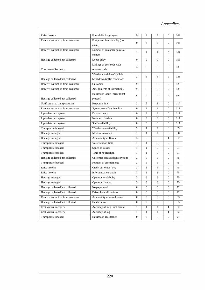
Appendices
220
Raise invoice Port of discharge agent 9 9 1 0 169
Receive instruction from customer Equipment functionality (fax
email) 9 3 9 0 165
Receive instruction from customer Number of customer points of
contact 1 9 9 0 161
Haulage collected/not collected Depot delay 0 9 9 0 153
Cost versus Recovery
Linkage of cost code with
revenue code 3 3 9 3 138
Haulage collected/not collected
Weather conditions/ vehicle
breakdown/traffic conditions 3 3 3 9 138
Receive instruction from customer Customer 9 3 3 0 123
Receive instruction from customer Amendments of instructions 9 3 3 0 123
Haulage collected/not collected
Hazardous labels (present/not
present) 9 3 3 0 123
Notification to transport team Response time 3 3 9 0 117
Receive instruction from customer System setup/functionality 0 9 3 0 111
Input data into system Data accuracy 0 9 3 0 111
Input data into system Number of orders 0 9 3 0 111
Input data into system Staff availability 0 9 3 0 111
Transport re-booked Warehouse availability 9 1 1 0 89
Haulage arranged Mode of transport 1 1 1 9 88
Haulage arranged Availability of Haulier 3 3 3 1 82
Transport re-booked Vessel cut off time 1 1 9 0 81
Transport re-booked Space on vessel 1 1 9 0 81
Transport re-booked Time of notification 1 1 9 0 81
Haulage collected/not collected Customer contact details (yes/no) 3 3 3 0 75
Transport re-booked Number of amendments 3 3 3 0 75
Raise invoice Credit customer (y/n) 3 3 3 0 75
Raise invoice Information on credit 3 3 3 0 75
Haulage arranged Operator availability 3 3 3 0 75
Haulage arranged Operator training 3 3 3 0 75
Haulage collected/not collected No paper work 0 3 3 3 72
Haulage collected/not collected Driver hour allocations 0 3 3 3 72
Receive instruction from customer Availability of vessel space 0 0 9 0 63
Haulage collected/not collected Haulier error 0 0 9 0 63
Cost versus Recovery Accuracy of info from haulier 1 1 1 1 32
Cost versus Recovery Accuracy of log 1 1 1 1 32
Transport re-booked Hazardous acceptance 0 0 3 0 21

Appendices
221
Appendix 2 FMEA analysis for non-recovered wasted journey

Appendices
222
Key Process
Input
Failure Modes -
What can go wrong?
Effects SE
V
Causes OC
C
Current
Controls
DE
T
RP
N
Container
suitability
Customer did not
request specific
container details
Wasted journey
(customer or
company liability)
10 Customer makes
assumptions that
container will be
suitable
8 No current
control
9 720
Container
suitability
Information not put on
booking
Wasted Journey
not recoverable
10 Human error 7 No current
control
9 630
accuracy of
info
Wrong date or time
relayed
Wasted Journey
company liable
10 Human error 7 No current
control
9 630
accuracy of
info
Wrong size container Wasted journey
company liable
10 Operator error,
info not put on
6 No current
control
9 540
accuracy of
info
Load Reference not
given
Wasted journey or
detention
8 Customer does not
give reference
7 No current
control
9 504
Time of day Cancellation received
close to midday and
relayed to transport
after 12
Wasted Journey
liable to company
10 Cut off of 12 and
customers utilise
every second.
5 No formal
controls
9 450
Quality of
notification of
failure
Conflicting info from
different departments
Difficulty in
wasted journey
recovery
10 Wrong info
relayed (transport)
7 Unknown 6 420
Operator
experience
Wrong data inputted Wasted journeys 10 Lack of
supervisory time
8 No current
control
5 400
Container
suitability
Box not available Wasted Journey
due to either
company or Depot
6 Unknown damage
to box's and
equipment
7 Depot
controls
/container
control
9 378
Accuracy of
info
Special trailer
requirements missed
Wasted Journey
customer
8 Information not
given by customer
5 No controls 9 360
Accuracy of
info
Special trailer
requirements missed
Wasted journey to
company
10 Operator error info
not put on
4 No current
control
9 360
Accuracy of
info
No special
requirements
Wasted Journey
company liable
10 Customer assumes
company
knowledge for
repeat business
4 No current
control
9 360
Type of
Instructions
Email and fax not
functioning
Delays
cancellation
causing wasted
journey
10 Server issues/
failures
4 No current
control
9 360
Operator
experience
Wrong data inputted Wasted journeys 10 Staff Shortages 7 No current
control
5 350
Container
suitability
Box not available wasted Journey
due to either
company or Depot
8 Box not released
(data accuracy)
4 Depot
controls
/container
control
9 288
Time of job Late for pick up Dispute with
customer
(accepted or
rejected)
5 Late on previous
job
8 No current
control
7 280
Container
suitability
Depot releases box not
to request standard
Wasted journey
fault of depot
6 Data accuracy and
stock control
5 Depot
controls
/container
control
9 270
Accuracy of
info
Wrong pick up point
info
Wasted Journey
company liable
10 Repeat bookings
with changed
address
3 No current
control
9 270
Accuracy of
info
Wrong pick up point
info
Wasted Journey
company liable
10 Places with same
name, transport do
not book on postal
code
3 No current
control
9 270

Appendices
223
Accuracy of
info
Wrong size container Wasted Journey
Customer
6 Customer error
(wrong info)
5 No current
control
9 270
Time of job Late for pick up Dispute with
customer
(accepted or
rejected)
5 Collecting empty
from depot due to
opening hours/ or
in stack
7 No current
control
7 245
Container
suitability
Customer did not
request specific
container details
Wasted journeys 8 Lack of customer
knowledge
3 No current
control
9 216
Accuracy of
info
Undeclared out of
gauge
Wasted journey to
customer
8 Customer does not
declare or give
accurate
measurements
3 No current
control
9 216
Operator
experience
Wrong data inputted Wasted journeys 10 Lack of training 5 Limited
training
4 200
Container
suitability
Information not put on
booking.
Wasted Journey
not recoverable
10 Lack of
Knowledge of
Customer Service
2 No current
control
9 180
Quality of
notification of
failure
Delay in customer
notification
Difficulty in
wasted journey
recovery
8 Delayed info from
transport (costs)
4 No current
control
4 128
Quality of
notification of
failure
Delay in customer
notification
Difficulty in
wasted journey
recovery
8 Lack of time in
customer service
department
4 No current
control
4 128
Accuracy of
info
Un-booked Hazard
and/or no stickers
Wasted journey to
customer
6 customer does not
declare as hazard
2 Responsibili
ty of
customer
9 108
Accuracy of
info
Un-booked Hazard
and/or no stickers
Wasted journey to
company
10 Operator error info
not put in system
1 No current
control
9 90
Accuracy of
info
Undeclared out of
gauge
Wasted journey to
company
10 Operator error info
not put in system
1 No current
control
9 90

Appendices
224
Appendix 3 FRB with Belief Structures and Weights of Criteria in
FMEA from Case Study
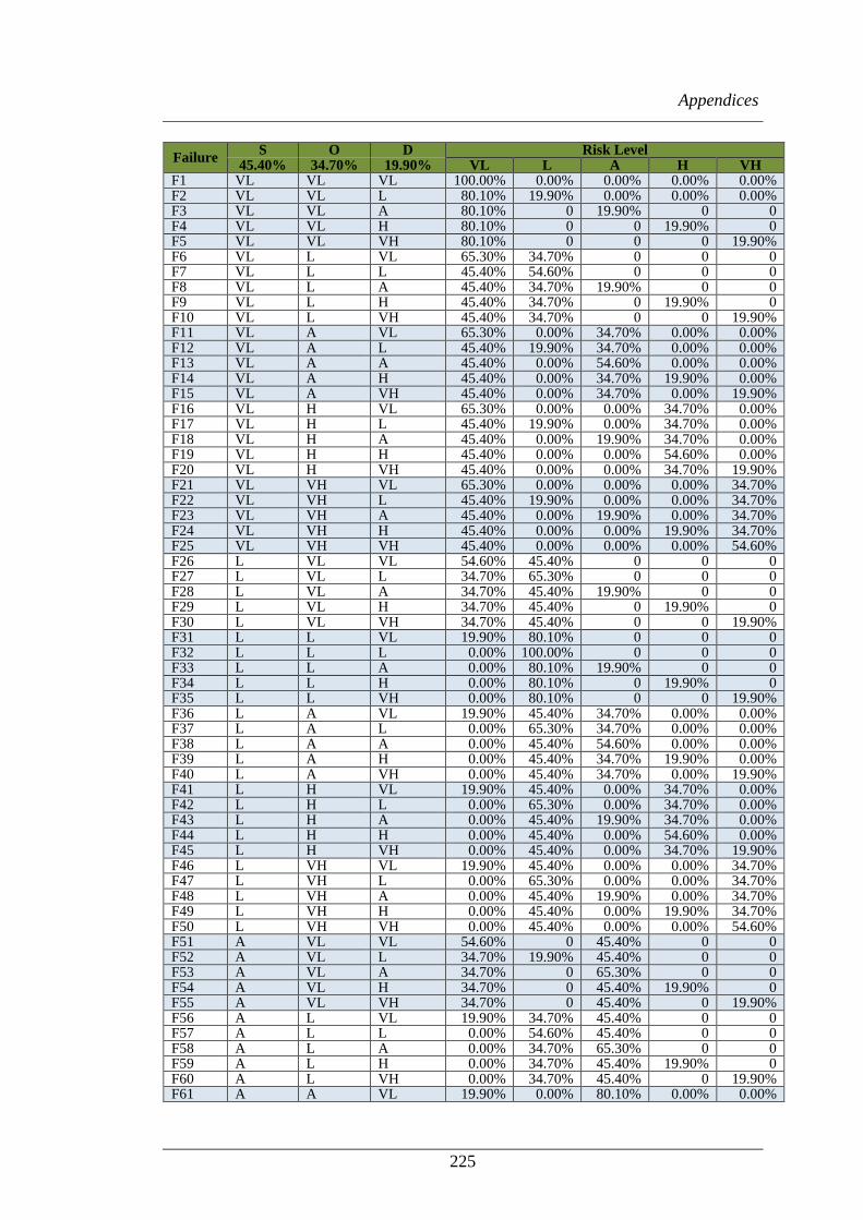
Appendices
225
Failure S O D Risk Level
45.40% 34.70% 19.90% VL L A H VH F1 VL VL VL 100.00% 0.00% 0.00% 0.00% 0.00% F2 VL VL L 80.10% 19.90% 0.00% 0.00% 0.00% F3 VL VL A 80.10% 0 19.90% 0 0 F4 VL VL H 80.10% 0 0 19.90% 0 F5 VL VL VH 80.10% 0 0 0 19.90% F6 VL L VL 65.30% 34.70% 0 0 0 F7 VL L L 45.40% 54.60% 0 0 0 F8 VL L A 45.40% 34.70% 19.90% 0 0 F9 VL L H 45.40% 34.70% 0 19.90% 0 F10 VL L VH 45.40% 34.70% 0 0 19.90% F11 VL A VL 65.30% 0.00% 34.70% 0.00% 0.00% F12 VL A L 45.40% 19.90% 34.70% 0.00% 0.00% F13 VL A A 45.40% 0.00% 54.60% 0.00% 0.00% F14 VL A H 45.40% 0.00% 34.70% 19.90% 0.00% F15 VL A VH 45.40% 0.00% 34.70% 0.00% 19.90% F16 VL H VL 65.30% 0.00% 0.00% 34.70% 0.00% F17 VL H L 45.40% 19.90% 0.00% 34.70% 0.00% F18 VL H A 45.40% 0.00% 19.90% 34.70% 0.00% F19 VL H H 45.40% 0.00% 0.00% 54.60% 0.00% F20 VL H VH 45.40% 0.00% 0.00% 34.70% 19.90% F21 VL VH VL 65.30% 0.00% 0.00% 0.00% 34.70% F22 VL VH L 45.40% 19.90% 0.00% 0.00% 34.70% F23 VL VH A 45.40% 0.00% 19.90% 0.00% 34.70% F24 VL VH H 45.40% 0.00% 0.00% 19.90% 34.70% F25 VL VH VH 45.40% 0.00% 0.00% 0.00% 54.60% F26 L VL VL 54.60% 45.40% 0 0 0 F27 L VL L 34.70% 65.30% 0 0 0 F28 L VL A 34.70% 45.40% 19.90% 0 0 F29 L VL H 34.70% 45.40% 0 19.90% 0 F30 L VL VH 34.70% 45.40% 0 0 19.90% F31 L L VL 19.90% 80.10% 0 0 0 F32 L L L 0.00% 100.00% 0 0 0 F33 L L A 0.00% 80.10% 19.90% 0 0 F34 L L H 0.00% 80.10% 0 19.90% 0 F35 L L VH 0.00% 80.10% 0 0 19.90% F36 L A VL 19.90% 45.40% 34.70% 0.00% 0.00% F37 L A L 0.00% 65.30% 34.70% 0.00% 0.00% F38 L A A 0.00% 45.40% 54.60% 0.00% 0.00% F39 L A H 0.00% 45.40% 34.70% 19.90% 0.00% F40 L A VH 0.00% 45.40% 34.70% 0.00% 19.90% F41 L H VL 19.90% 45.40% 0.00% 34.70% 0.00% F42 L H L 0.00% 65.30% 0.00% 34.70% 0.00% F43 L H A 0.00% 45.40% 19.90% 34.70% 0.00% F44 L H H 0.00% 45.40% 0.00% 54.60% 0.00% F45 L H VH 0.00% 45.40% 0.00% 34.70% 19.90% F46 L VH VL 19.90% 45.40% 0.00% 0.00% 34.70% F47 L VH L 0.00% 65.30% 0.00% 0.00% 34.70% F48 L VH A 0.00% 45.40% 19.90% 0.00% 34.70% F49 L VH H 0.00% 45.40% 0.00% 19.90% 34.70% F50 L VH VH 0.00% 45.40% 0.00% 0.00% 54.60% F51 A VL VL 54.60% 0 45.40% 0 0 F52 A VL L 34.70% 19.90% 45.40% 0 0 F53 A VL A 34.70% 0 65.30% 0 0 F54 A VL H 34.70% 0 45.40% 19.90% 0 F55 A VL VH 34.70% 0 45.40% 0 19.90% F56 A L VL 19.90% 34.70% 45.40% 0 0 F57 A L L 0.00% 54.60% 45.40% 0 0 F58 A L A 0.00% 34.70% 65.30% 0 0 F59 A L H 0.00% 34.70% 45.40% 19.90% 0 F60 A L VH 0.00% 34.70% 45.40% 0 19.90% F61 A A VL 19.90% 0.00% 80.10% 0.00% 0.00%

Appendices
226
F62 A A L 0.00% 19.90% 80.10% 0.00% 0.00% F63 A A A 0.00% 0.00% 100.00% 0.00% 0.00% F64 A A H 0.00% 0.00% 80.10% 19.90% 0.00% F65 A A VH 0.00% 0.00% 80.10% 0.00% 19.90% F66 A H VL 19.90% 0.00% 45.40% 34.70% 0.00% F67 A H L 0.00% 19.90% 45.40% 34.70% 0.00% F68 A H A 0.00% 0.00% 65.30% 34.70% 0.00% F69 A H H 0.00% 0.00% 45.40% 54.60% 0.00% F70 A H VH 0.00% 0.00% 45.40% 34.70% 19.90% F71 A VH VL 19.90% 0.00% 45.40% 0.00% 34.70% F72 A VH L 0.00% 19.90% 45.40% 0.00% 34.70% F73 A VH A 0.00% 0.00% 65.30% 0.00% 34.70% F74 A VH H 0.00% 0.00% 45.40% 19.90% 34.70% F75 A VH VH 0.00% 0.00% 45.40% 0.00% 54.60% F76 H VL VL 54.60% 0 0 45.40% 0 F77 H VL L 34.70% 19.90% 0 45.40% 0 F78 H VL A 34.70% 0 19.90% 45.40% 0 F79 H VL H 34.70% 0 0 65.30% 0 F80 H VL VH 34.70% 0 0 45.40% 19.90% F81 H L VL 19.90% 34.70% 0.00% 45.40% 0.00% F82 H L L 0.00% 54.60% 0.00% 45.40% 0.00% F83 H L A 0.00% 34.70% 19.90% 45.40% 0.00% F84 H L H 0.00% 34.70% 0.00% 65.30% 0.00% F85 H L VH 0.00% 34.70% 0.00% 45.40% 19.90% F86 H A VL 19.90% 0.00% 34.70% 45.40% 0.00% F87 H A L 0.00% 19.90% 34.70% 45.40% 0.00% F88 H A A 0.00% 0.00% 54.60% 45.40% 0.00% F89 H A H 0.00% 0.00% 34.70% 65.30% 0.00% F90 H A VH 0.00% 0.00% 34.70% 45.40% 19.90% F91 H H VL 19.90% 0.00% 0.00% 80.10% 0.00% F92 H H L 0.00% 19.90% 0.00% 80.10% 0.00% F93 H H A 0.00% 0.00% 19.90% 80.10% 0.00% F94 H H H 0.00% 0.00% 0.00% 100.00% 0.00% F95 H H VH 0.00% 0.00% 0.00% 80.10% 19.90% F96 H VH VL 19.90% 0.00% 0.00% 45.40% 34.70% F97 H VH L 0.00% 19.90% 0.00% 45.40% 34.70% F98 H VH A 0.00% 0.00% 19.90% 45.40% 34.70% F99 H VH H 0.00% 0.00% 0.00% 65.30% 34.70% F100 H VH VH 0.00% 0.00% 0.00% 45.40% 54.60% F101 VH VL VL 54.60% 0 0 0 45.40% F102 VH VL L 34.70% 19.90% 0 0 45.40% F103 VH VL A 34.70% 0 19.90% 0 45.40% F104 VH VL H 34.70% 0 0 19.90% 45.40% F105 VH VL VH 34.70% 0 0 0 65.30% F106 VH L VL 19.90% 34.70% 0.00% 0.00% 45.40% F107 VH L L 0.00% 54.60% 0.00% 0.00% 45.40% F108 VH L A 0.00% 34.70% 19.90% 0.00% 45.40% F109 VH L H 0.00% 34.70% 0.00% 19.90% 45.40% F110 VH L VH 0.00% 34.70% 0.00% 0.00% 65.30% F111 VH A VL 19.90% 0.00% 34.70% 0.00% 45.40% F112 VH A L 0.00% 19.90% 34.70% 0.00% 45.40% F113 VH A A 0.00% 0.00% 54.60% 0.00% 45.40% F114 VH A H 0.00% 0.00% 34.70% 19.90% 45.40% F115 VH A VH 0.00% 0.00% 34.70% 0.00% 65.30% F116 VH H VL 19.90% 0.00% 0.00% 34.70% 45.40% F117 VH H L 0.00% 19.90% 0.00% 34.70% 45.40% F118 VH H A 0.00% 0.00% 19.90% 34.70% 45.40% F119 VH H H 0.00% 0.00% 0.00% 54.60% 45.40% F120 VH H VH 0.00% 0.00% 0.00% 34.70% 65.30% F121 VH VH VL 19.90% 0.00% 0.00% 0.00% 80.10% F122 VH VH L 0.00% 19.90% 0.00% 0.00% 80.10% F123 VH VH A 0.00% 0.00% 19.90% 0.00% 80.10% F124 VH VH H 0.00% 0.00% 0.00% 19.90% 80.10%

Appendices
227
F125 VH VH VH 0.00% 0.00% 0.00% 0.00% 100.00%

Appendices
228
Appendix 4 Questionnaire for DEMATEL Study Among KPIs

Appendices
229
School of Engineering
Section of Maritime Studies
Liverpool John Moores University
Byrom Street
L3 3AF
UK
Phone : 0044 (0)151 231 2028
Fax : 0044 (0)151 298 2624
Email : [email protected]
08 October 2014
Dear Sir/Madam,
With the ever increasing customer requirements level and global market competition,
companies are paying increasing attention to enhance their performance in order to
retain customers. Profitability along is not sufficient to discriminate excellence.
Therefore, measuring company performance in every aspect becomes an important part
of today’s business management. As one of the performance measurement tools, Key
Performance Indicators (KPIs) are widely used in practice as a freestanding tool or part
of process improvement methodology.
A research project at Liverpool John Moores University is currently being carried out
with regard to KPIs management in shipping industry. The necessity for this
investigation is that at the moment, most companies that uses KPIs only use them to
measure numerical inputs, but not or very limited where qualitative information
presents. This has made KPIs become measures for what can be measured instead of
what needs to be measured. Furthermore, if effectively used, KPIs can be used as great
bases for performance benchmarking and comparisons.
This research aims at develop a KPIs management method using techniques that can
effectively handle qualitative data and take into account of the weights and relationship
of different KPIs so that they can be eventually synthesized into comparable units.
Our research now needs to test if the newly developed method can serve the research
aims. Thus this survey sets out for collecting information to be used in the method. For
the purpose of this research, existing KPIs in your company are adopted.
I should be most grateful if I could ask you to spare some of your very valuable time to
complete the accompanying questionnaire and to email or post it to myself at the
address as shown above. Your vital feedback will greatly benefit and contribute in the
formulation of an industry wide opinion. I can assure you that the confidentiality of
your response will be honoured and respected.

Appendices
230
Yours faithfully,
Zhuohua Qu
Lead Researcher
MSc, B.Eng (Hons) Maritime Operations
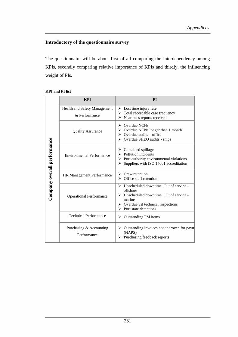
Appendices
231
Introductory of the questionnaire survey
The questionnaire will be about first of all comparing the interdependency among
KPIs, secondly comparing relative importance of KPIs and thirdly, the influencing
weight of PIs.
KPI and PI list
Com
pan
y o
ver
all
per
form
an
ce
KPI PI
Health and Safety Management
& Performance
Lost time injury rate
Total recordable case frequency
Near miss reports received
Quality Assurance
Overdue NCNs
Overdue NCNs longer than 1 month
Overdue audits – office
Overdue SHEQ audits - ships
Environmental Performance
Contained spillage
Pollution incidents
Port authority environmental violations
Suppliers with ISO 14001 accreditation
HR Management Performance Crew retention
Office staff retention
Operational Performance
Unscheduled downtime. Out of service -
offshore
Unscheduled downtime. Out of service -
marine
Overdue vsl technical inspections
Port state detentions
Technical Performance Outstanding PM items
Purchasing & Accounting
Performance
Outstanding invoices not approved for payment
(NAPS)
Purchasing feedback reports

Appendices
232
The objective of this questionnaire is to identify any interdependency among KPIs.
Description on how to fill up the Questionnaire
The evaluation scale of interdependency between indicators ranges from 0 to 3 as
show in the table below.
Evaluation scale and its corresponding degree of agree
0 No influence
1 Low influence
2 Medium influence
3 High influence
4 Very high influence
Example - how to evaluate the interdependency of indicators and fill the blanks
of the Evaluation Forms for indicators
This Evaluation Form attempts to draw your evaluation on the level of influence
among KPIs. For example, among 7 KPIs, if you think that the performance of PIs in
KPI B (Quality Assurance) has high influence on the performance of target KPI A
(Health and Safety Management & Performance), your evaluation scale is “3” so
that you should mark “X” in “3” against KPI B on the evaluation form as below.
Sample Form:
Target KPI: (A) Health and Safety Management & Performance
KPI Degree of influencing
0 1 2 3 4
(B) Quality Assurance X
However, if you think that the performance of PIs in KPI B (Quality Assurance)
has no influence on the performance of targeting KPI A (Health and Safety
Management & Performance), your evaluation scale is “0” so that you should mark
“X” in “0” against KPI B on the evaluation form as below.

Appendices
233
Sample Form:
Target KPI: (A) Health and Safety Management & Performance
KPI Degree of influencing
0 1 2 3 4
(B) Quality Assurance X

Appendices
234
Evaluation form of the influence level between KPIs (Questionnaire to be filled)
Degree of influence that each of the following KPI directly has on the target KPI:
(A)Health and Safety Management & Performance
KPI
Degree of influencing
0: No influence, 1:Low influence
2:Medium influence: 3: High
influence
4:Very high influence
0 1 2 3 4
(B)Quality Assurance
(C)Environmental Performance
(D)HR Management Performance
(E)Operational Performance
(F)Technical Performance
(G)Purchasing & Accounting Performance
Degree of influence that each of the following KPI directly has on the target KPI:
(B)Quality Assurance
KPI
Degree of influencing
0: No influence, 1:Low influence
2:Medium influence: 3: High
influence
4:Very high influence
0 1 2 3 4
(A)Health and Safety Management & Performance
(C)Environmental Performance
(D)HR Management Performance
(E)Operational Performance
(F)Technical Performance
(G)Purchasing & Accounting Performance

Appendices
235
Degree of influence that each of the following KPI directly has on the target KPI:
(C)Environmental Performance
KPI
Degree of influencing
0: No influence, 1:Low influence
2:Medium influence: 3: High
influence
4:Very high influence
0 1 2 3 4
(A)Health and Safety Management & Performance
(B)Quality Assurance
(D)HR Management Performance
(E)Operational Performance
(F)Technical Performance
(G)Purchasing & Accounting Performance
Degree of influence that each of the following KPI directly has on the target KPI:
(D)HR Management Performance
KPI
Degree of influencing
0: No influence, 1:Low influence
2:Medium influence: 3: High
influence
4:Very high influence
0 1 2 3 4
(A)Health and Safety Management & Performance
(B)Quality Assurance
(C)Environmental Performance
(E)Operational Performance
(F)Technical Performance
(G)Purchasing & Accounting Performance
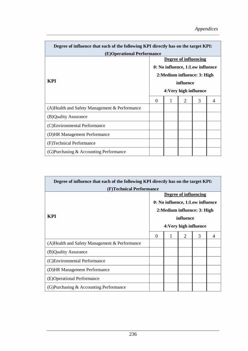
Appendices
236
Degree of influence that each of the following KPI directly has on the target KPI:
(E)Operational Performance
KPI
Degree of influencing
0: No influence, 1:Low influence
2:Medium influence: 3: High
influence
4:Very high influence
0 1 2 3 4
(A)Health and Safety Management & Performance
(B)Quality Assurance
(C)Environmental Performance
(D)HR Management Performance
(F)Technical Performance
(G)Purchasing & Accounting Performance
Degree of influence that each of the following KPI directly has on the target KPI:
(F)Technical Performance
KPI
Degree of influencing
0: No influence, 1:Low influence
2:Medium influence: 3: High
influence
4:Very high influence
0 1 2 3 4
(A)Health and Safety Management & Performance
(B)Quality Assurance
(C)Environmental Performance
(D)HR Management Performance
(E)Operational Performance
(G)Purchasing & Accounting Performance
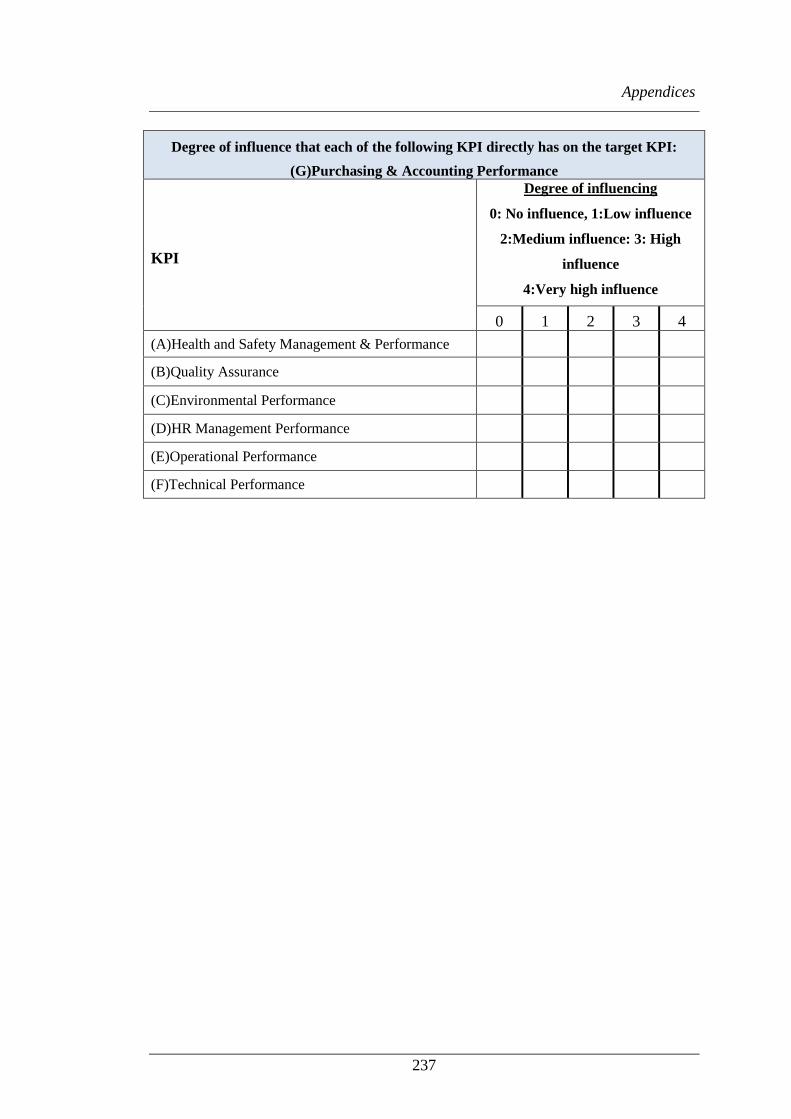
Appendices
237
Degree of influence that each of the following KPI directly has on the target KPI:
(G)Purchasing & Accounting Performance
KPI
Degree of influencing
0: No influence, 1:Low influence
2:Medium influence: 3: High
influence
4:Very high influence
0 1 2 3 4
(A)Health and Safety Management & Performance
(B)Quality Assurance
(C)Environmental Performance
(D)HR Management Performance
(E)Operational Performance
(F)Technical Performance

Appendices
238
Appendix 5 Questionnaire for ANP Study to Obtain the Evaluation
for the Importance of Indicators in Relation to the Upper Level
Indicators

Appendices
239
The objective is to identify the importance of KPIs and PIs in relation to their upper-
level indicators.
Description on how to fill up the Questionnaire
The evaluation scale of weights of criteria ranges from 1 to 9 depending on the
degree of relative importance as shown in the table below.
Evaluation scale and its corresponding degree of importance
Evaluation scale Degree of importance
1 Equally Important to the objective
3 Slightly more important to the objective
5 Moderately more important to the objective
7 Strongly more important to the objective
9 Absolutely more important to the objective
2, 4, 6, 8 are intermediate values between the two adjacent judgements
Example - how to evaluate the relative importance of criteria and fill the blanks
of the Evaluation Form for KPIs
Our Evaluation Form attempts to draw your evaluation on relative importance of
KPIs and PIs between the first left hand and the last right hand columns. In other
words, it aims to identify how much more relatively important the KPIs or PIs in the
first left hand column are compared to those in the last right hand column for every
row to the objective, and vice versa.
For example, if you think KPI A (Health and Safety Management & Performance)
in the first LEFT hand column is more important than KPI B (Quality Assurance)
in the last RIGHT hand column in contributing to the objective - company overall
performance, then please tick “X” in “A” (as below in blue). After that, if you think
that A is moderately more important than B, your evaluation scale is “5” so that
you should circle the 5:1 column of the Evaluation Form below. (See our Sample
Form below)

Appendices
240
Sample Form:
KPI
(Absolutely more important:9、Strongly more important:7、
Moderately more important:5、Slightly more important: 3、
Equally Important:1) KPI
In case that KPI in first LEFT hand
column are relatively more important
than the KPI in the last right hand
column, circle an appropriate column
according to your importance
evaluation scale
Equally
important
In case that KPI in last RIGHT
hand column are relatively more
important than the KPI in the first
LEFT hand column, circle an
appropriate column according to
your importance evaluation scale
(A) Health and
Safety Management
& Performance (X)
9:1 8:1 7:1
6:1
5:1 4:1 3:1 2:1 1:1 1:2 1:3 1:4 1:5 1:6 1:7 1:8 1:9
(B) Quality
Assurance ( )
On the contrary, if you think KPI B (Quality Assurance) in the last RIGHT hand
column is more important than KPI A (Health and Safety Management &
Performance) in the first LEFT hand column in contributing to the objective -
company overall performance, then please tick “X” in “B” (as below in blue). After
that, if you think that B is Strongly more important than A, your evaluation scale is
“7” so that you should circle the 1:7 column of the Evaluation Form below. (See our
Sample Form below)
Sample Form:
KPI
(Absolutely more important:9、Strongly more important:7、
Moderately more important:5、Slightly more important: 3、
Equally Important:1) KPI
In case that KPI in first LEFT hand
column are relatively more important
than the KPI in the last right hand
column, circle an appropriate column
according to your importance
evaluation scale Equally
important
In case that KPI in last RIGHT
hand column are relatively
more important than the KPI in
the first LEFT hand column,
circle an appropriate column
according to your importance
evaluation scale
(A) Health and
Safety Management
& Performance ( )
9:1 8:1 7:1 6:1 5:1 4:1 3:1 2:1 1:1 1:2 1:3 1:4 1:5 1:6
1:7
1:8 1:9
(B) Quality
Assurance (X)
Next, if you think the importance of any KPI or PI is located between “Strongly
more important (the scale 7)” and “Absolutely more important (the scale 9)” to the
objective, compared to other KPI or PI, your evaluation scale is 8 so that please

Appendices
241
circle the 8:1 or 1:8 column. This logical scale evaluation is applied to evaluation
scales, 2, 4, 6, and 8.
Finally, if your think that the importance of KPIs between A in the first left hand
column and B in the last right hand column are the same (“Equally Important”) to the
objective, your evaluation scale is 1, please circle only in the 1:1 column in the
middle of the Evaluation Form. (See our Sample Form below)
Sample Form:
KPI
(Absolutely more important:9、Strongly more important:7、
Moderately more important:5、Slightly more important: 3、
Equally Important:1) KPI
In case that KPI in first LEFT hand
column are relatively more important
than the KPI in the last right hand
column, circle an appropriate column
according to your importance
evaluation scale
Equall
y
import
ant
In case that KPI in last RIGHT
hand column are relatively more
important than the KPI in the first
LEFT hand column, circle in an
appropriate column according to
your importance evaluation scale
(A) Health and
Safety Management
& Performance ( )
9:1 8:1 7:1 6:1 5:1 4:1 3:1 2:1
1:1 1:2 1:3 1:4 1:5 1:6 1:7 1:8 1:9
(B) Quality
Assurance ( )
In the same way as explained above, all the comparison on each row SHOULD be
filled with one of the evaluation scale numbers ranging from 1 to 9 according to
your judgment of weights between each pair of criteria.

Appendices
242
Evaluation form of the importance of all indicators in relation to the upper level
indicators (Questionnaire to be filled)
Objective - Company overall performance
KPI
(Absolutely more important:9、Strongly more important:7、
Moderately more important:5、Slightly more important: 3、
Equally Important:1)
KPI
In case that KPI in first LEFT
hand column is relatively
more important than the KPI
in the last right hand column,
circle an appropriate column
according to your evaluation
scale Equally
important
In case that KPI in last
RIGHT hand column is
relatively more important
than the criteria in the first
LEFT hand column, circle an
appropriate column
according to your evaluation
scale (A)Health and Safety Management & Performance ( )
9:1 8:1 7:1 6:1 5:1 4:1 3:1 2:1 1:1 1:2 1:3 1:4 1:5 1:6 1:7 1:8 1:9
(B)Quality Assurance ( )
(A)Health and Safety Management & Performance ( )
9:1 8:1 7:1 6:1 5:1 4:1 3:1 2:1 1:1 1:2 1:3 1:4 1:5 1:6 1:7 1:8 1:9
(C)Environmental Performance ( )
(A)Health and Safety Management & Performance ( )
9:1 8:1 7:1 6:1 5:1 4:1 3:1 2:1 1:1 1:2 1:3 1:4 1:5 1:6 1:7 1:8 1:9
(D)HR Management Performance ( )
(A)Health and Safety Management & Performance ( )
9:1 8:1 7:1 6:1 5:1 4:1 3:1 2:1 1:1 1:2 1:3 1:4 1:5 1:6 1:7 1:8 1:9
(E)Operational Performance ( )
(A)Health and Safety Management & Performance ( )
9:1 8:1 7:1 6:1 5:1 4:1 3:1 2:1 1:1 1:2 1:3 1:4 1:5 1:6 1:7 1:8 1:9
(F)Technical Performance ( )
(A)Health and Safety Management & Performance ( )
9:1 8:1 7:1 6:1 5:1 4:1 3:1 2:1 1:1 1:2 1:3 1:4 1:5 1:6 1:7 1:8 1:9
(G)Purchasing & Accounting Performance ( )
(B)Quality Assurance ( )
9:1 8:1 7:1 6:1 5:1 4:1 3:1 2:1 1:1 1:2 1:3 1:4 1:5 1:6 1:7 1:8 1:9 (C)Environmental Performance ( )
(B)Quality Assurance ( ) 9:1 8:1 7:1 6:1 5:1 4:1 3:1 2:1 1:1 1:2 1:3 1:4 1:5 1:6 1:7 1:8 1:9
(D)HR Management Performance ( )
(B)Quality Assurance ( )
9:1 8:1 7:1 6:1 5:1 4:1 3:1 2:1 1:1 1:2 1:3 1:4 1:5 1:6 1:7 1:8 1:9 (E)Operational Performance ( )
(B)Quality Assurance ( )
9:1 8:1 7:1 6:1 5:1 4:1 3:1 2:1 1:1 1:2 1:3 1:4 1:5 1:6 1:7 1:8 1:9 (F)Technical Performance ( )
(B)Quality Assurance ( ) 9:1 8:1 7:1 6:1 5:1 4:1 3:1 2:1 1:1 1:2 1:3 1:4 1:5 1:6 1:7 1:8 1:9
(G)Purchasing & Accounting Performance ( )
(C)Environmental Performance ( ) 9:1 8:1 7:1 6:1 5:1 4:1 3:1 2:1 1:1 1:2 1:3 1:4 1:5 1:6 1:7 1:8 1:9
(D)HR Management Performance ( )
(C)Environmental Performance ( )
9:1 8:1 7:1 6:1 5:1 4:1 3:1 2:1 1:1 1:2 1:3 1:4 1:5 1:6 1:7 1:8 1:9 (E)Operational Performance ( )
(C)Environmental Performance ( )
9:1 8:1 7:1 6:1 5:1 4:1 3:1 2:1 1:1 1:2 1:3 1:4 1:5 1:6 1:7 1:8 1:9 (F)Technical Performance ( )
(C)Environmental Performance ( ) 9:1 8:1 7:1 6:1 5:1 4:1 3:1 2:1 1:1 1:2 1:3 1:4 1:5 1:6 1:7 1:8 1:9
(G)Purchasing & Accounting Performance ( )

Appendices
243
(D)HR Management Performance ( )
9:1 8:1 7:1 6:1 5:1 4:1 3:1 2:1 1:1 1:2 1:3 1:4 1:5 1:6 1:7 1:8 1:9
(E)Operational Performance ( )
(D)HR Management Performance ( )
9:1 8:1 7:1 6:1 5:1 4:1 3:1 2:1 1:1 1:2 1:3 1:4 1:5 1:6 1:7 1:8 1:9
(F)Technical Performance ( )
(D)HR Management Performance ( )
9:1 8:1 7:1 6:1 5:1 4:1 3:1 2:1 1:1 1:2 1:3 1:4 1:5 1:6 1:7 1:8 1:9
(G)Purchasing & Accounting Performance ( )
(E)Operational Performance ( )
9:1 8:1 7:1 6:1 5:1 4:1 3:1 2:1 1:1 1:2 1:3 1:4 1:5 1:6 1:7 1:8 1:9 (F)Technical Performance ( )
(E)Operational Performance ( ) 9:1 8:1 7:1 6:1 5:1 4:1 3:1 2:1 1:1 1:2 1:3 1:4 1:5 1:6 1:7 1:8 1:9
(G)Purchasing & Accounting Performance ( )
(F)Technical
Performance ( ) 9:1 8:1 7:1 6:1 5:1 4:1 3:1 2:1 1:1 1:2 1:3 1:4 1:5 1:6 1:7 1:8 1:9
(G)Purchasing &
Accounting
KPI (A) Health and Safety Management & Performance
PI
(Absolutely more important:9、Strongly more important:7、
Moderately more important:5、Slightly more important: 3、
Equally Important:1)
PI In case that KPI in first LEFT hand
column are relatively more
important than the KPI in the last
right hand column, circle an
appropriate column according to
your importance evaluation scale Equally
important
In case that KPI in last RIGHT hand
column are relatively more important
than the criteria in the first LEFT
hand column, circle an appropriate
column according to your
importance evaluation scale (A1)Lost Time Injury Rate ( )
9:1 8:1 7:1 6:1 5:1 4:1 3:1 2:1 1:1 1:2 1:3 1:4 1:5 1:6 1:7 1:8 1:9
(A2)Total Recordable Case Frequency ( )
(A1)Lost Time Injury Rate ( )
9:1 8:1 7:1 6:1 5:1 4:1 3:1 2:1 1:1 1:2 1:3 1:4 1:5 1:6 1:7 1:8 1:9
(A3)Near Miss Reports received ( )
(A2)Total Recordable Case Frequency ( )
9:1 8:1 7:1 6:1 5:1 4:1 3:1 2:1 1:1 1:2 1:3 1:4 1:5 1:6 1:7 1:8 1:9
(A3)Near Miss Reports received ( )

Appendices
244
KPI (B) Quality Assurance
PI
(Absolutely more important:9、Strongly more important:7、
Moderately more important:5、Slightly more important: 3、
Equally Important:1)
PI
In case that KPI in first LEFT hand
column are relatively more important
than the KPI in the last right hand
column, circle an appropriate column
according to your importance
evaluation scale Equally
important
In case that KPI in last RIGHT
hand column are relatively more
important than the criteria in the
first LEFT hand column, mark
circle an appropriate column
according to your importance
evaluation scale (B1)Overdue NCNs ( ) 9:1 8:1 7:1 6:1 5:1 4:1 3:1 2:1 1:1 1:2 1:3 1:4 1:5 1:6 1:7 1:8 1:9
(B2)Overdue NCNs longer than 1 month ( )
(B1)Overdue NCNs ( ) 9:1 8:1 7:1 6:1 5:1 4:1 3:1 2:1 1:1 1:2 1:3 1:4 1:5 1:6 1:7 1:8 1:9
(B3)Overdue Audits - Office ( )
(B1)Overdue NCNs ( ) 9:1 8:1 7:1 6:1 5:1 4:1 3:1 2:1 1:1 1:2 1:3 1:4 1:5 1:6 1:7 1:8 1:9
(B4)Overdue SHEQ Audits - Ships ( )
(B2)Overdue NCNs longer than 1 month ( )
9:1 8:1 7:1 6:1 5:1 4:1 3:1 2:1 1:1 1:2 1:3 1:4 1:5 1:6 1:7 1:8 1:9
(B3)Overdue Audits - Office ( )
(B2)Overdue NCNs longer than 1 month ( )
9:1 8:1 7:1 6:1 5:1 4:1 3:1 2:1 1:1 1:2 1:3 1:4 1:5 1:6 1:7 1:8 1:9
(B4)Overdue SHEQ Audits - Ships ( )
(B3)Overdue Audits - Office ( )
9:1 8:1 7:1 6:1 5:1 4:1 3:1 2:1 1:1 1:2 1:3 1:4 1:5 1:6 1:7 1:8 1:9
(B4)Overdue SHEQ Audits - Ships ( )
KPI (C) Environmental Performance
PI
(Absolutely more important:9、Strongly more important:7、
Moderately more important:5、Slightly more important: 3、
Equally Important:1)
PI In case that KPI in first LEFT hand
column are relatively more important
than the KPI in the last right hand
column, circle an appropriate column
according to your importance
evaluation scale Equally
important
In case that KPI in last RIGHT
hand column are relatively more
important than the criteria in the
first LEFT hand column, circle an
appropriate column according to
your importance evaluation scale (C1)Contained Spillage ( )
9:1 8:1 7:1 6:1 5:1 4:1 3:1 2:1 1:1 1:2 1:3 1:4 1:5 1:6 1:7 1:8 1:9 (C2)Pollution Incidents ( )
(C1)Contained Spillage ( )
9:1 8:1 7:1 6:1 5:1 4:1 3:1 2:1 1:1 1:2 1:3 1:4 1:5 1:6 1:7 1:8 1:9
(C3)Port Authority Environmental Violations ( )
(C1)Contained Spillage ( ) 9:1 8:1 7:1 6:1 5:1 4:1 3:1 2:1 1:1 1:2 1:3 1:4 1:5 1:6 1:7 1:8 1:9
(C4)Suppliers With ISO 14001 Accreditation ( )
(C2)Pollution Incidents ( )
9:1 8:1 7:1 6:1 5:1 4:1 3:1 2:1 1:1 1:2 1:3 1:4 1:5 1:6 1:7 1:8 1:9
(C3)Port Authority Environmental Violations ( )
(C2)Pollution Incidents ( ) 9:1 8:1 7:1 6:1 5:1 4:1 3:1 2:1 1:1 1:2 1:3 1:4 1:5 1:6 1:7 1:8 1:9
(C4)Suppliers With ISO 14001 Accreditation ( )
(C3)Port Authority Environmental Violations ( )
9:1 8:1 7:1 6:1 5:1 4:1 3:1 2:1 1:1 1:2 1:3 1:4 1:5 1:6 1:7 1:8 1:9
(C4)Suppliers With ISO 14001 Accreditation ( )

Appendices
245
KPI (D) HR Management Performance
PI
(Absolutely more important:9、Strongly more important:7、
Moderately more important:5、Slightly more important: 3、
Equally Important:1)
PI In case that KPI in first LEFT hand
column are relatively more important
than the KPI in the last right hand
column, circle an appropriate column
according to your importance
evaluation scale Equally
important
In case that KPI in last RIGHT
hand column are relatively more
important than the criteria in the
first LEFT hand column, circle an
appropriate column according to
your importance evaluation scale (D1)Crew Retention ( ) 9:1 8:1 7:1 6:1 5:1 4:1 3:1 2:1 1:1 1:2 1:3 1:4 1:5 1:6 1:7 1:8 1:9
(D2)Office Staff retention ( )
KPI (E) Operational Performance
PI
(Absolutely more important:9、Strongly more important:7、
Moderately more important:5、Slightly more important: 3、
Equally Important:1)
PI In case that KPI in first LEFT hand
column are relatively more
important than the KPI in the last
right hand column, circle an
appropriate column according to
your importance evaluation scale
Equall
y
import
ant
In case that KPI in last RIGHT hand
column are relatively more
important than the criteria in the
first LEFT hand column, circle an
appropriate column according to
your importance evaluation scale (E1)Unscheduled downtime. Out of Service - Offshore ( )
9:1 8:1 7:1 6:1 5:1 4:1 3:1 2:1 1:1 1:2 1:3 1:4 1:5 1:6 1:7 1:8 1:9
(E2)Unscheduled downtime. Out of Service - Marine ( )
(E1)Unscheduled downtime. Out of Service - Offshore ( )
9:1 8:1 7:1 6:1 5:1 4:1 3:1 2:1 1:1 1:2 1:3 1:4 1:5 1:6 1:7 1:8 1:9
(E3)Overdue Vsl Technical Inspections ( )
(E1)Unscheduled downtime. Out of Service - Offshore ( )
9:1 8:1 7:1 6:1 5:1 4:1 3:1 2:1 1:1 1:2 1:3 1:4 1:5 1:6 1:7 1:8 1:9
(E4)Port State Detentions ( )
(E2)Unscheduled downtime. Out of Service - Marine ( )
9:1 8:1 7:1 6:1 5:1 4:1 3:1 2:1 1:1 1:2 1:3 1:4 1:5 1:6 1:7 1:8 1:9
(E3)Overdue Vsl Technical Inspections ( )
(E2)Unscheduled downtime. Out of Service - Marine ( )
9:1 8:1 7:1 6:1 5:1 4:1 3:1 2:1 1:1 1:2 1:3 1:4 1:5 1:6 1:7 1:8 1:9
(E4)Port State Detentions ( )
(E3)Overdue Vsl Technical Inspections ( )
9:1 8:1 7:1 6:1 5:1 4:1 3:1 2:1 1:1 1:2 1:3 1:4 1:5 1:6 1:7 1:8 1:9
(E4)Port State Detentions ( )
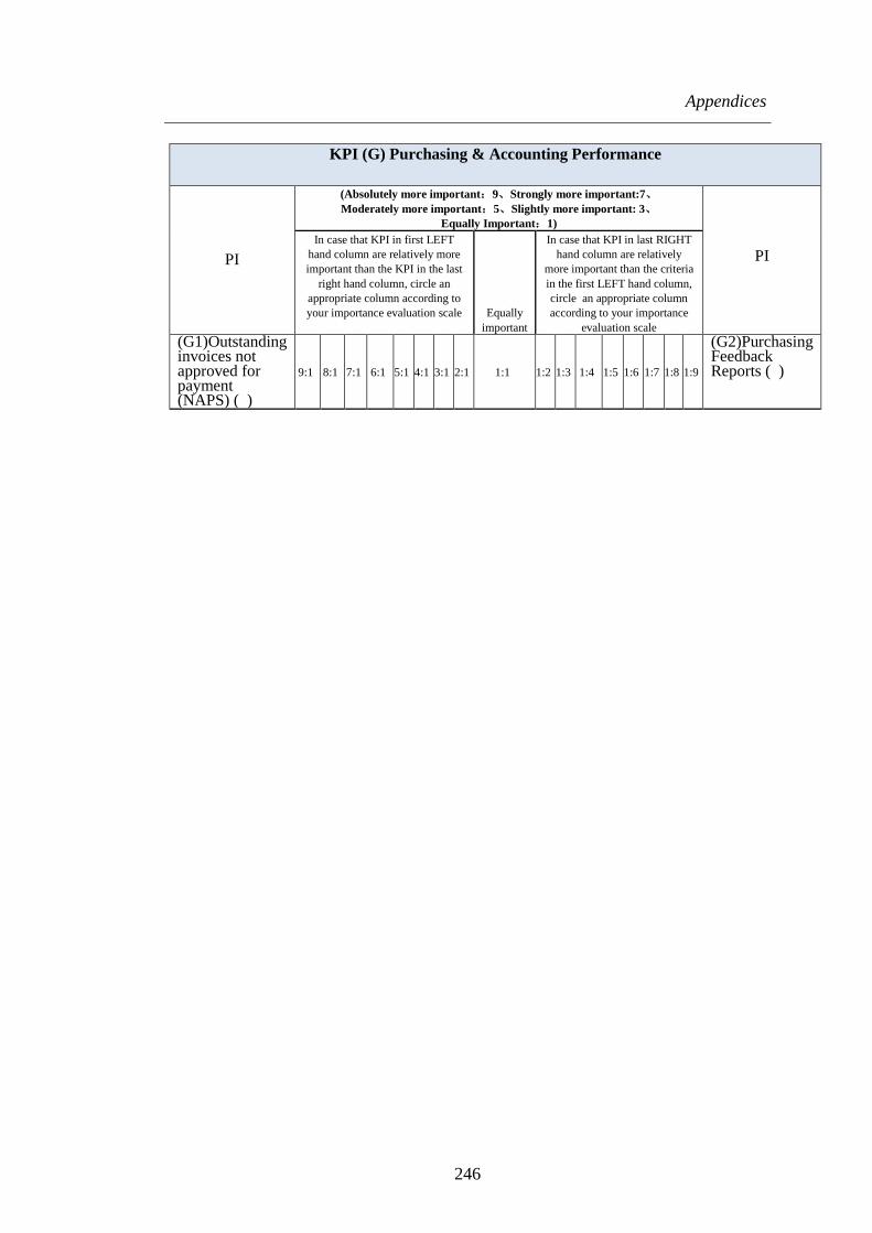
Appendices
246
KPI (G) Purchasing & Accounting Performance
PI
(Absolutely more important:9、Strongly more important:7、
Moderately more important:5、Slightly more important: 3、
Equally Important:1)
PI In case that KPI in first LEFT
hand column are relatively more
important than the KPI in the last
right hand column, circle an
appropriate column according to
your importance evaluation scale Equally
important
In case that KPI in last RIGHT
hand column are relatively
more important than the criteria
in the first LEFT hand column,
circle an appropriate column
according to your importance
evaluation scale (G1)Outstanding invoices not approved for payment (NAPS) ( )
9:1 8:1 7:1 6:1 5:1 4:1 3:1 2:1 1:1 1:2 1:3 1:4 1:5 1:6 1:7 1:8 1:9
(G2)Purchasing Feedback Reports ( )

Appendices
247
Appendix 6 Questionnaire for ANP Study to Obtain the Evaluation for the
Level of Influences among Lower Level Indicators

Appendices
248
This questionnaire will be about finding interdependencies weights among all
indicators.
Description on how to fill up the Questionnaire
The evaluation scale of influencing level of indicators ranges from 1 to 9. The
followings describe the used scale of Relative Influence level of two elements with
respect to another given element:
Evaluation scale and its corresponding degree of influence
Evaluation scale Degree of importance
1 Equal Influence
3 Moderate Influence
5 Essential or Strong Influence
7 Substantial Influence
9 Extreme Influence
2, 4, 6, 8 are intermediate values between the two adjacent judgements
Example - how to evaluate the relative influence level of indicators and fill the
blanks of the Evaluation Forms
For example, if you think KPI B (Quality Assurance) is more influential than KPI
C (Environmental Performance) on a common given criteria “KPI A (Health and
Safety Management & Performance)” in achieving the objective – better
company performance, then please tick “X” in “B” (as below in blue). Next, if you
think “KPI B” influences “KPI A” 5 times more than the unselected KPI C – then
circle or highlight “5” in any colour at the side of selected KPI B.

Appendices
249
Sample Form:
which of the two indicator influences (A) Health and Safety Management & Performance
more with respect to the Company Performance, and how much more than another
indicator
KPI
(Extreme Influence:9、Substantial Influence:7、
Essential or Strong Influence:5、Moderate Influence: 3、
Equal Influence:1)
KPI
(B) Quality Assurance (
X ) 9 8 7 6 5 4 3 2 1 2 3 4 5 6 7 8 9
(C) Environmental
Performance
On the contrary, if you think KPI C (Environmental Performance) is more
influential than KPI B (Quality Assurance) on a common given criteria “KPI A
(Health and Safety Management & Performance)” in achieving the objective –
better company performance, then please tick “X” in “C” (as below in blue). Next,
if you think “KPI C” influences “KPI A” 9 times more than the unselected KPI B –
then circle or highlight “9” in any colour at the side of selected KPI A.
Sample Form:
which of the two indicator influences (A) Health and Safety Management & Performance
more with respect to the Company Performance, and how much more than another
indicator
KPI
(Extreme Influence:9、Substantial Influence:7、
Essential or Strong Influence:5、Moderate Influence: 3、
Equal Influence:1)
KPI
(B) Quality Assurance (
) 9 8 7 6 5 4 3 2 1 2 3 4 5 6 7 8 9
(C) Environmental
Performance (X)
Finally, you might notice that there are situations where the indicators to be
compared are the same as the common given criteria. For example, compare KPI B
(Quality Assurance) with KPI C (Environmental Performance) to decide which
one is more influential on KPI B (Quality Assurance) in achieving the objective –
better company performance. In such situation, if KPI C has little influence on KPI
B in respect to the objective and the performance of KPI B in regards to the objective
is highly influenced by its own performance, then, KPI B might be 7 or 8 times more
influential than KPI C (depending on your judgement). However, If KPI C has strong

Appendices
250
influence on KPI B than KPI B itself in regards to the objective , then the score to
choose will be “5”for KPI C.
In the same way as explained above, all the comparison on each row SHOULD be
filled with one of the evaluation scale numbers ranging from 1 to 9 according to
your judgment of the level of influence between each two criteria.

Appendices
251
Evaluation form of the influence level among indicators (Questionnaire to be
filled)
Which indicator in the pair (on the same row) influences A2) Total Recordable Case Frequency more with respect to the (A) Health and Safety Management &
Performance, and how much more than the other indicator No.
PI (Extreme Influence:9、Substantial Influence:7、
Essential or Strong Influence:5、Moderate Influence: 3、
Equal Influence:1)
PI
1 (C1)Contained Spillage ( )
9 8 7 6 5 4 3 2 1 2 3 4 5 6 7 8 9 (C2)Pollution Incidents ( )
2
(C1)Contained Spillage ( ) 9 8 7 6 5 4 3 2 1 2 3 4 5 6 7 8 9
(C3)Port Authority Environmental Violations ( )
3
(C2)Pollution Incidents ( ) 9 8 7 6 5 4 3 2 1 2 3 4 5 6 7 8 9
(C3)Port Authority Environmental Violations ( )
Which indicator in the pair (on the same row) influences B1) Overdue NCNs more with respect to the (B) Quality Assurance, and how much more than the other indicator
No.
PI
(Extreme Influence:9、Substantial Influence:7、
Essential or Strong Influence:5、Moderate Influence:
3、
Equal Influence:1)
PI
4
(B2)Overdue NCNs longer than 1 month ( )
9 8 7 6 5 4 3 2 1 2 3 4 5 6 7 8 9
(B4)Overdue SHEQ Audits - Ships ( )
5
(E3)Overdue Vsl Technical Inspections ( )
9 8 7 6 5 4 3 2 1 2 3 4 5 6 7 8 9
(E4)Port State Detentions ( )
Which indicator in the pair (on the same row) influences B2) Overdue NCNs longer than 1 month more with respect to the (B) Quality Assurance, and how much more than
the other indicator No.
PI (Extreme Influence:9、Substantial Influence:7、
Essential or Strong Influence:5、Moderate Influence: 3、
Equal Influence:1)
PI
6
(B1)Overdue NCNs ( ) 9 8 7 6 5 4 3 2 1 2 3 4 5 6 7 8 9
(B4)Overdue SHEQ Audits - Ships ( )
Which indicator in the pair (on the same row) influences C1) Contained Spillage more with respect to the (C) Environmental Performance, and how much more than the
other indicator No.
PI
(Extreme Influence:9、Substantial Influence:7、
Essential or Strong Influence:5、Moderate Influence:
3、
Equal Influence:1)
PI
7
(B1)Overdue NCNs ( ) 9 8 7 6 5 4 3 2 1 2 3 4 5 6 7 8 9
(B2)Overdue NCNs longer than 1 month ( )
8
(B1)Overdue NCNs ( ) 9 8 7 6 5 4 3 2 1 2 3 4 5 6 7 8 9
(B4)Overdue SHEQ Audits - Ships ( )
9
(B2)Overdue NCNs longer than 1 month ( )
9 8 7 6 5 4 3 2 1 2 3 4 5 6 7 8 9
(B4)Overdue SHEQ Audits - Ships ( )
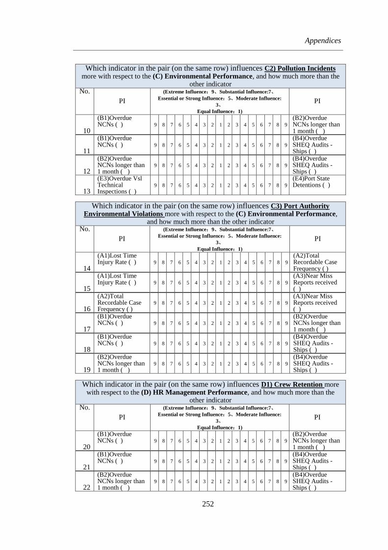
Appendices
252
Which indicator in the pair (on the same row) influences C2) Pollution Incidents more with respect to the (C) Environmental Performance, and how much more than the
other indicator No.
PI
(Extreme Influence:9、Substantial Influence:7、
Essential or Strong Influence:5、Moderate Influence:
3、
Equal Influence:1)
PI
10
(B1)Overdue NCNs ( ) 9 8 7 6 5 4 3 2 1 2 3 4 5 6 7 8 9
(B2)Overdue NCNs longer than 1 month ( )
11
(B1)Overdue NCNs ( ) 9 8 7 6 5 4 3 2 1 2 3 4 5 6 7 8 9
(B4)Overdue SHEQ Audits - Ships ( )
12
(B2)Overdue NCNs longer than 1 month ( )
9 8 7 6 5 4 3 2 1 2 3 4 5 6 7 8 9
(B4)Overdue SHEQ Audits - Ships ( )
13
(E3)Overdue Vsl Technical Inspections ( )
9 8 7 6 5 4 3 2 1 2 3 4 5 6 7 8 9
(E4)Port State Detentions ( )
Which indicator in the pair (on the same row) influences C3) Port Authority
Environmental Violations more with respect to the (C) Environmental Performance, and how much more than the other indicator
No.
PI
(Extreme Influence:9、Substantial Influence:7、
Essential or Strong Influence:5、Moderate Influence:
3、
Equal Influence:1)
PI
14
(A1)Lost Time Injury Rate ( ) 9 8 7 6 5 4 3 2 1 2 3 4 5 6 7 8 9
(A2)Total Recordable Case Frequency ( )
15
(A1)Lost Time Injury Rate ( ) 9 8 7 6 5 4 3 2 1 2 3 4 5 6 7 8 9
(A3)Near Miss Reports received ( )
16
(A2)Total Recordable Case Frequency ( )
9 8 7 6 5 4 3 2 1 2 3 4 5 6 7 8 9
(A3)Near Miss Reports received ( )
17
(B1)Overdue NCNs ( ) 9 8 7 6 5 4 3 2 1 2 3 4 5 6 7 8 9
(B2)Overdue NCNs longer than 1 month ( )
18
(B1)Overdue NCNs ( ) 9 8 7 6 5 4 3 2 1 2 3 4 5 6 7 8 9
(B4)Overdue SHEQ Audits - Ships ( )
19
(B2)Overdue NCNs longer than 1 month ( )
9 8 7 6 5 4 3 2 1 2 3 4 5 6 7 8 9
(B4)Overdue SHEQ Audits - Ships ( )
Which indicator in the pair (on the same row) influences D1) Crew Retention more
with respect to the (D) HR Management Performance, and how much more than the other indicator
No.
PI
(Extreme Influence:9、Substantial Influence:7、
Essential or Strong Influence:5、Moderate Influence:
3、
Equal Influence:1)
PI
20
(B1)Overdue NCNs ( ) 9 8 7 6 5 4 3 2 1 2 3 4 5 6 7 8 9
(B2)Overdue NCNs longer than 1 month ( )
21
(B1)Overdue NCNs ( ) 9 8 7 6 5 4 3 2 1 2 3 4 5 6 7 8 9
(B4)Overdue SHEQ Audits - Ships ( )
22
(B2)Overdue NCNs longer than 1 month ( )
9 8 7 6 5 4 3 2 1 2 3 4 5 6 7 8 9
(B4)Overdue SHEQ Audits - Ships ( )

Appendices
253
Which indicator in the pair (on the same row) influences E1) Unscheduled downtime. Out of Service – Offshore more with respect to the (E) Operational
Performance, and how much more the than other indicator No.
PI
(Extreme Influence:9、Substantial Influence:7、
Essential or Strong Influence:5、Moderate Influence:
3、
Equal Influence:1)
PI
23 (C1)Contained Spillage ( )
9 8 7 6 5 4 3 2 1 2 3 4 5 6 7 8 9 (C2)Pollution Incidents ( )
24
(C1)Contained Spillage ( ) 9 8 7 6 5 4 3 2 1 2 3 4 5 6 7 8 9
(C3)Port Authority Environnemental Violations ( )
25
(C2)Pollution Incidents ( ) 9 8 7 6 5 4 3 2 1 2 3 4 5 6 7 8 9
(C3)Port Authority Environnemental Violations ( )
Which indicator in the pair (on the same row) influences E2) Unscheduled downtime. Out of Service – Marine more with respect to the (E) Operational
Performance, and how much more than the other indicator No.
PI
(Extreme Influence:9、Substantial Influence:7、
Essential or Strong Influence:5、Moderate Influence:
3、
Equal Influence:1)
PI
26 (C1)Contained Spillage ( )
9 8 7 6 5 4 3 2 1 2 3 4 5 6 7 8 9 (C2)Pollution Incidents ( )
27
(C1)Contained Spillage ( ) 9 8 7 6 5 4 3 2 1 2 3 4 5 6 7 8 9
(C3)Port Authority Environnemental Violations ( )
28
(C2)Pollution Incidents ( ) 9 8 7 6 5 4 3 2 1 2 3 4 5 6 7 8 9
(C3)Port Authority Environnemental Violations ( )
Which indicator in the pair (on the same row) influences E3) Overdue Vsl Technical Inspections more with respect to the (E) Operational Performance, and how much more
than the other indicator No.
PI
(Extreme Influence:9、Substantial Influence:7、
Essential or Strong Influence:5、Moderate Influence:
3、
Equal Influence:1)
PI
29
(B1)Overdue NCNs ( ) 9 8 7 6 5 4 3 2 1 2 3 4 5 6 7 8 9
(B2)Overdue NCNs longer than 1 month ( )
30 (B1)Overdue NCNs ( )
9 8 7 6 5 4 3 2 1 2 3 4 5 6 7 8 9 (B4)Overdue SHEQ Audits - Ships ( )
31
(B2)Overdue NCNs longer than 1 month ( )
9 8 7 6 5 4 3 2 1 2 3 4 5 6 7 8 9
(B4)Overdue SHEQ Audits - Ships ( )
32 (C1)Contained Spillage ( )
9 8 7 6 5 4 3 2 1 2 3 4 5 6 7 8 9 (C2)Pollution Incidents ( )
33
(C1)Contained Spillage ( ) 9 8 7 6 5 4 3 2 1 2 3 4 5 6 7 8 9
(C3)Port Authority Environnemental Violations ( )
34
(C2)Pollution Incidents ( ) 9 8 7 6 5 4 3 2 1 2 3 4 5 6 7 8 9
(C3)Port Authority Environnemental Violations ( )

Appendices
254
Which indicator in the pair (on the same row) influences E4) Port State Detentions more with respect to the (E) Operational Performance, and how much more than the other
indicator No.
PI (Extreme Influence:9、Substantial Influence:7、
Essential or Strong Influence:5、Moderate Influence:3、
Equal Influence:1)
PI
35
(A1)Lost Time Injury Rate ( ) 9 8 7 6 5 4 3 2 1 2 3 4 5 6 7 8 9
(A2)Total Recordable Case Frequency ( )
36 (C1)Contained Spillage ( )
9 8 7 6 5 4 3 2 1 2 3 4 5 6 7 8 9 (C2)Pollution Incidents ( )
37
(C1)Contained Spillage ( ) 9 8 7 6 5 4 3 2 1 2 3 4 5 6 7 8 9
(C3)Port Authority Environnemental Violations ( )
38
(C1)Contained Spillage ( ) 9 8 7 6 5 4 3 2 1 2 3 4 5 6 7 8 9
(C4)Suppliers With ISO 14001 Accreditation ( )
39
(C2)Pollution Incidents ( ) 9 8 7 6 5 4 3 2 1 2 3 4 5 6 7 8 9
(C3)Port Authority Environnemental Violations ( )
40
(C2)Pollution Incidents ( ) 9 8 7 6 5 4 3 2 1 2 3 4 5 6 7 8 9
(C4)Suppliers With ISO 14001 Accreditation ( )
41
(C3)Port Authority Environnemental Violations ( )
9 8 7 6 5 4 3 2 1 2 3 4 5 6 7 8 9
(C4)Suppliers With ISO 14001 Accreditation ( )
Which indicator in the pair (on the same row) influences F1) Outstanding PM Items more with respect to the F) Technical Performance, and how much more than the other
indicator No.
PI (Extreme Influence:9、Substantial Influence:7、
Essential or Strong Influence:5、Moderate Influence:3、
Equal Influence:1)
PI
42
(B1)Overdue NCNs ( ) 9 8 7 6 5 4 3 2 1 2 3 4 5 6 7 8 9
(B2)Overdue NCNs longer than 1 month ( )
43 (B1)Overdue NCNs ( )
9 8 7 6 5 4 3 2 1 2 3 4 5 6 7 8 9 (B4)Overdue SHEQ Audits - Ships ( )
44
(B2)Overdue NCNs longer than 1 month ( )
9 8 7 6 5 4 3 2 1 2 3 4 5 6 7 8 9
(B4)Overdue SHEQ Audits - Ships ( )
45 (C1)Contained Spillage ( )
9 8 7 6 5 4 3 2 1 2 3 4 5 6 7 8 9 (C2)Pollution Incidents ( )
46
(C1)Contained Spillage ( ) 9 8 7 6 5 4 3 2 1 2 3 4 5 6 7 8 9
(C3)Port Authority Environnemental Violations ( )
47
(C2)Pollution Incidents ( ) 9 8 7 6 5 4 3 2 1 2 3 4 5 6 7 8 9
(C3)Port Authority Environnemental Violations ( )
48
(E1)Unscheduled downtime. Out of Service - Offshore ( )
9 8 7 6 5 4 3 2 1 2 3 4 5 6 7 8 9
(E2)Unscheduled downtime. Out of Service - Marine ( )
49
(E1)Unscheduled downtime. Out of Service - Offshore ( )
9 8 7 6 5 4 3 2 1 2 3 4 5 6 7 8 9
(E4)Port State Detentions ( )
50
(E2)Unscheduled downtime. Out of Service - Marine ( )
9 8 7 6 5 4 3 2 1 2 3 4 5 6 7 8 9
(E4)Port State Detentions ( )