analytical solution of constrained lq optimal … solution of constrained lq optimal control for...
TRANSCRIPT

Analytical Solution of Constrained LQ OptimalControl for Horizon 2
Jose De Dona
September 2004
Centre of Complex DynamicSystems and Control

Outline
1 A Motivating ExampleCautious DesignSerendipitous DesignTactical Design
2 Explicit SolutionsExplicit vs Implicit
3 A Simple Problem with N = 2Dynamic Programming
4 Motivating Example Revisited
5 Conclusions
Centre of Complex DynamicSystems and Control

A Motivating Example
Consider the double integrator plant:
d2y(t)dt2
= u(t).
The zero-order hold discretisation with sampling period 1 is:
xk+1 = Axk + Buk ,
yk = Cxk ,
with
A =
[1 10 1
], B =
[0.51
], C =
[1 0
].
Assume the actuator has a maximum and minimum allowed value(saturation) of ±1. Thus, the controller has to satisfy the constraint:|uk | ≤ 1 for all k .
Centre of Complex DynamicSystems and Control

A Motivating Example
The schematic of the feedback control loop is shown in the Figure.
uk xkcontroller linear
systemsat
Figure: Feedback control loop.
“sat” represents the actuator modelled by the saturation function
sat(u) =
⎧⎪⎪⎪⎪⎪⎨⎪⎪⎪⎪⎪⎩1 if u > 1,
u if |u| ≤ 1,
−1 if u < −1.
Centre of Complex DynamicSystems and Control
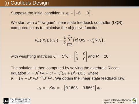
(i) Cautious Design
Suppose the initial condition is x0 =[−6 0
]t.
We start with a “low gain” linear state feedback controller (LQR),computed so as to minimise the objective function:
V∞({xk }, {uk }) = 12
∞∑k=0
(xtk Qxk + utk Ruk
),
with weighting matrices Q = CtC =
[1 00 0
]and R = 20.
The solution is then computed by solving the algebraic Riccatiequation P = A tPA + Q − K t(R + BtPB)K, whereK = (R + BtPB)−1BtPA. We obtain the linear state feedback law:
uk = −Kxk = −[0.1603 0.5662
]xk .
Centre of Complex DynamicSystems and Control

(i) Cautious Design
“Slow gain” control: Q = CtC =
[1 00 0
], R = 20, uk = −Kxk .
The resulting input and output sequences are shown in the Figure.
0 5 10 15 20 25−0.4
−0.2
0
0.2
0.4
0.6
0.8
1
0 5 10 15 20 25−6
−5
−4
−3
−2
−1
0
1
k
k
u ky k
We can see from the figure thatthe input uk satisfies the givenconstraint |uk | ≤ 1, for all k ; forthis initial condition.
The response is rather slow. The“settling time” is of the order of 8samples.
Centre of Complex DynamicSystems and Control

(ii) Serendipitous Design
“High gain” control: Q = CtC =
[1 00 0
], R = 2, uk = sat(−Kxk ).
The resulting input and output sequences are shown in the Figure.
0 5 10 15 20 25−1
0
1
2
3
0 5 10 15 20 25−6
−5
−4
−3
−2
−1
0
1
k
k
u ky k
We can see from the figure thatthe input uk satisfies the givenconstraint |uk | ≤ 1, for all k . Thecontroller makes better use of theavailable control authority.
The amount of overshoot isessentially the same. The“settling time” is of the order of 5samples.
Centre of Complex DynamicSystems and Control

(ii) Serendipitous Design
“High gain” control: Q = CtC =
[1 00 0
], R = 0.1, uk = sat(−Kxk ).
The resulting input and output sequences are shown in the Figure.
0 5 10 15 20 25−6
−4
−2
0
2
4
6
0 5 10 15 20 25−6
−4
−2
0
2
4
k
k
u ky k
We can see from the figure thatthe input uk satisfies the givenconstraint |uk | ≤ 1, for all k . Thecontrol sequence stays saturatedmuch longer.
Significant overshoot. The“settling time” blows out to 12samples.
Centre of Complex DynamicSystems and Control

Recapitulation
Going from R = 20→ 2: same overshoot, faster response.
Going from R = 2→ 0.1: large overshoot, long settling time.
Let us examine the state space trajectory corresponding to theserendipitous strategy R = 0.1, uk = sat(−Kxk ):
−6 −4 −2 0 2 4 6−4
−3
−2
−1
0
1
2
3
4
x1k
x2 k
R0
R1
R2
The control law u = −sat(Kx)partitions the state space intothree regions. Hence, thecontroller can be characterisedas a switched control strategy:
u = K(x) =
⎧⎪⎪⎪⎪⎪⎨⎪⎪⎪⎪⎪⎩−Kx if x ∈ R0,
1 if x ∈ R1,
−1 if x ∈ R2.
Centre of Complex DynamicSystems and Control

Recapitulation
−6 −4 −2 0 2 4 6−4
−3
−2
−1
0
1
2
3
4
x1k
x2 k
R0
R1
R2
u = K(x) =
⎧⎪⎪⎪⎪⎪⎨⎪⎪⎪⎪⎪⎩−Kx if x ∈ R0,
1 if x ∈ R1,
−1 if x ∈ R2.
Heuristically, we can think,in thisexample, of x2 as “velocity” andx1 as “position.” Now, in ourattempt to change the positionrapidly (from −6 to 0), the velocityhas been allowed to grow to arelatively high level (+3). Thiswould be fine if the braking actionwere unconstrained. However,our input (including braking) islimited to the range [−1, 1].Hence, the available braking isinadequate to “pull the systemup,” and overshoot occurs.
Centre of Complex DynamicSystems and Control

(iii) Tactical Design
We will now start “afresh” with a formulation that incorporatesconstraints from the beginning in the design process.
A sensible idea would seem to be to try to “look ahead” and takeaccount of future input constraints (that is, the limited brakingauthority available).
We now consider a Model Predictive Control law with predictionhorizon N = 2. At each sampling instant i and for the current statexi, the two-step objective function:
V2({xk }, {uk }) = 12
xti+2Pxi+2 +12
i+1∑k=i
(xtk Qxk + utk Ruk
), (1)
is minimised subject to the equality and inequality constraints:
xk+1 = Axk + Buk , k = i, i + 1,
|uk | ≤ 1, k = i, i + 1.(2)
Centre of Complex DynamicSystems and Control
(iii) Tactical Design
In the objective function (1), we set, as before, Q = CtC, R = 0.1.The terminal state weighting matrix P is taken to be the solution ofthe algebraic Riccati equation P = A tPA + Q − K t(R + BtPB)K,where K = (R + BtPB)−1BtPA.
As a result of minimising (1) subject the constraints (2), we obtainan optimal fixed-horizon control sequence
{uopti , uopti+1}
We then apply the resulting value of uopti to the system in areceding horizon control form.
We can see that this strategy has the ability to “look ahead” byconsidering the constraints not only at the current time i, but alsoone step ahead i + 1.
Centre of Complex DynamicSystems and Control

(iii) Tactical Design
MPC: Q = CtC =
[1 00 0
], R = 0.1, Horizon N = 2
The resulting input and output sequences are shown in the Figure.
0 5 10 15 20 25−6
−4
−2
0
2
4
6
0 5 10 15 20 25−6
−4
−2
0
2
4
k
k
u ky k
Dashed line: control uk = −Kxk .Solid line: MPC
We can see from the figure thatthe output trajectory withconstrained input now hasminimal overshoot. Thus, theidea of “looking ahead” has paiddividends.
Centre of Complex DynamicSystems and Control

Recapitulation
As we will see in this part of the course, the receding horizoncontrol strategy (MPC) we have used can be described as apartition of the state space into different regions in which affinecontrol laws hold.
Serendipitous strategyR = 0.1, uk = sat(−Kxk ).
−6 −4 −2 0 2 4 6−4
−3
−2
−1
0
1
2
3
4
x1k
x2 k
R0
R1
R2
Receding horizon tacticaldesign R = 0.1, N = 2.
−6 −4 −2 0 2 4 6−4
−3
−2
−1
0
1
2
3
4
x1k
x2 k
R0
R1
R2
R3
R4
Centre of Complex DynamicSystems and Control

Explicit vs Implicit
Before we start studying how to find an explicit characterisation ofthe MPC solution, let us first define what procedures we would callexplicit and which ones we would call implicit.
Explicit solution(p = parameter,a, b = constants).
fp(z) = z2 + 2apz + bp
z∂fp∂z = 0⇒ zopt(p) = −ap
Implicit (numerical)solution (p = parameter,a, b = constants).
fp(z) = z2 + 2apz + bp
zz0pzk
pzk+1p
. . .
Centre of Complex DynamicSystems and Control

Problem Setup
We consider the discrete time system
xk+1 = Axk + Buk ,
where xk ∈ Rn and uk ∈ R. The pair (A ,B) is assumed to bestabilisable. We consider the following fixed horizon optimal controlproblem:
PN(x) : VoptN (x) = min VN({xk }, {uk }), (3)
subject to: x0 = x,
xk+1 = Axk + Buk for k = 0, 1, . . . ,N − 1,
uk ∈ U = [−∆,∆] for k = 0, 1, . . . ,N − 1,
where ∆ > 0 is the input constraint level. The objective function is:
VN({xk }, {uk }) = 12
xtNPxN +12
N−1∑k=0
(xtk Qxk + utk Ruk
). (4)
Centre of Complex DynamicSystems and Control

Problem Setup
Let the control sequence that achieves the minimum in (3) be:
{uopt0 , uopt1 , . . . , u
optN−1}
The Receding horizon control law, which depends on the currentstate x = x0, is
KN(x) = uopt0 .
Can we obtain an explicit expression for KN(·) defined above,as a function of the parameter x?
Centre of Complex DynamicSystems and Control

A Simple Problem with N = 2
Consider now the following fixed horizon optimal control problemwith prediction horizon N = 2:
P2(x) : Vopt2 (x) = min V2({xk }, {uk }), (5)
subject to: x0 = x
xk+1 = Axk + Buk for k = 0, 1,
uk ∈ U = [−∆,∆] for k = 0, 1.
The objective function in (5) is
V2({xk }, {uk }) = 12
xt2Px2 +12
1∑k=0
(xtk Qxk + utk Ruk
).
Centre of Complex DynamicSystems and Control

A Simple Problem with N = 2
Objective function:
V2({xk }, {uk }) = 12
xt2Px2 +12
1∑k=0
(xtk Qxk + utk Ruk
). (6)
The matrices Q and R are assumed positive semi-definite anddefinite respectively. P is taken as the solution to the algebraicRiccati equation
P = A tPA + Q − K tRK ,
where K = R−1BtPA, R = R + BtPB.Let the control sequence that minimises (6) be
{uopt0 , uopt1 }.
Then the RHC law is given by the first element of the optimalsequence (which depends on the current state x0 = x), that is,
K2(x) = uopt0 .
Centre of Complex DynamicSystems and Control
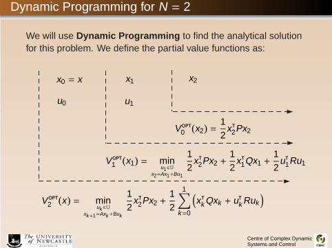
Dynamic Programming for N = 2
We will use Dynamic Programming to find the analytical solutionfor this problem. We define the partial value functions as:
x0 = x x1 x2
u1u0
Vopt0 (x2) =12
xt2Px2
Vopt1 (x1) = minu1∈U
x2=Ax1+Bu1
12
xt2Px2 +12
xt1Qx1 +12
ut1Ru1
Vopt2 (x) = minuk ∈U
xk+1=Axk +Buk
12
xt2Px2 +12
1∑k=0
(xtk Qxk + utk Ruk
)
Centre of Complex DynamicSystems and Control
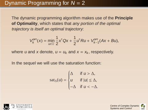
Dynamic Programming for N = 2
The dynamic programming algorithm makes use of the Principleof Optimality, which states that any portion of the optimaltrajectory is itself an optimal trajectory:
Voptk (x) = minu∈U
12
xtQx +12
utRu + Voptk−1(Ax + Bu),
where u and x denote, u = uk and x = xk , respectively.
In the sequel we will use the saturation function:
sat∆(u) =
⎧⎪⎪⎪⎪⎪⎨⎪⎪⎪⎪⎪⎩∆ if u > ∆,
u if |u| ≤ ∆,−∆ if u < −∆.
Centre of Complex DynamicSystems and Control

Dynamic Programming for N = 2
Theorem (RHC Characterisation for N = 2)
The RHC law has the form
K2(x) =
⎧⎪⎪⎪⎪⎪⎨⎪⎪⎪⎪⎪⎩−sat∆(Gx + h) if x ∈ Z−,−sat∆(Kx) if x ∈ Z,−sat∆(Gx − h) if x ∈ Z+,
(7)
where the gains K ,G ∈ R1×n and the constant h ∈ R are
K = R−1BtPA , G =K + KBKA1 + (KB)2
, h =KB
1 + (KB)2∆,
and the sets (Z−,Z,Z+) are defined by
Z− = {x : K (A − BK )x < −∆} , Z = {x : |K (A − BK )x | ≤ ∆} ,Z+ = {x : K (A − BK )x > ∆} .
Centre of Complex DynamicSystems and Control

Dynamic Programming for N = 2
Outline of the Proof:
(i) The partial value function Vopt0 :Here x = x2. By definition, the partial value function at timek = N = 2 is
Vopt0 (x) =12
xtPx for all x ∈ Rn.
(ii) The partial value function Vopt1 :Here x = x1 and u = u1. By the principle of optimality, for all x ∈ Rn,
Vopt1 (x) = minu∈U
{12
xtQx +12
utRu + Vopt0 (Ax + Bu)
}
= minu∈U
{12
xtQx +12
utRu +12
(Ax + Bu)tP(Ax + Bu)
}
= minu∈U
{12
xtPx +12
R(u + Kx)2}.
Centre of Complex DynamicSystems and Control

Dynamic Programming for N = 2
Vopt1 (x) = minu∈U
{12
xtPx +12
R(u + Kx)2}.
12xtPx + 1
2 R(u + Kx)2
uuopt1 = −Kx
12xtPx + 1
2R(u + Kx)2
−Kx uuopt1
From the convexity of the function R(u + Kx)2 it then follows thatthe constrained (u ∈ U) optimal control law is given by
uopt1 = sat∆(−Kx) = −sat∆(Kx) for all x ∈ Rn.
Centre of Complex DynamicSystems and Control

Dynamic Programming for N = 2
Substituting the optimal control
uopt1 = −sat∆(Kx) for all x ∈ Rn.
into the minimisation problem
Vopt1 (x) = minu∈U
{12
xtPx +12
R(u + Kx)2}.
we have that the partial value function at time k = N − 1 = 1 is
Vopt1 (x) =12
xtPx +12
R [Kx − sat∆(Kx)]2 for all x ∈ Rn.
Centre of Complex DynamicSystems and Control

Dynamic Programming for N = 2
(iii) The partial value function Vopt2 :Here x = x0 and u = u0. By the principle of optimality, we havethat, for all x ∈ Rn,
Vopt2 (x) = minu∈U
{12
xtQx +12
utRu + Vopt1 (Ax + Bu)
}
= minu∈U
{12
xtQx +12
utRu +12
(Ax + Bu)tP(Ax + Bu)
+12
R [K (Ax + Bu) − sat∆(K (Ax + Bu))]2}
=12
minu∈U{xtPx + R(u + Kx)2
+ R [KAx + KBu − sat∆(KAx + KBu)]2}.
Centre of Complex DynamicSystems and Control

Dynamic Programming for N = 2
uopt0 = arg minu∈U{ f1(u)︷��������︸︸��������︷R(u + Kx)2 +
f2(u)︷�������������������������������������������︸︸�������������������������������������������︷R [KAx + KBu − sat∆(KAx + KBu)]2
}.
Case (a): x ∈ Z−
x ∈ Z−
⇔KAx + KB(−Kx) < −∆
f1(u)f2(u)
f1(u) + f2(u)
−Kx u
Centre of Complex DynamicSystems and Control

Dynamic Programming for N = 2
We conclude that
uopt0 = arg minu∈U{R(u + Kx)2 + R [KAx + KBu − sat∆(KAx + KBu)]2
}
= arg minu∈U{R(u + Kx)2 + R [KAx + KBu + ∆]2
}
Hence
uopt0 = −sat∆(Gx + h) for all x ∈ Z−,where
G =K + KBKA1 + (KB)2
, h =KB
1 + (KB)2∆.
Centre of Complex DynamicSystems and Control

Dynamic Programming for N = 2
uopt0 = arg minu∈U{ f1(u)︷��������︸︸��������︷R(u + Kx)2 +
f2(u)︷�������������������������������������������︸︸�������������������������������������������︷R [KAx + KBu − sat∆(KAx + KBu)]2
}.
Case (b): x ∈ Z
x ∈ Z⇔|KAx + KB(−Kx)| ≤ ∆
f1(u)
f2(u)
f1(u) + f2(u)
−Kx u
Centre of Complex DynamicSystems and Control

Dynamic Programming for N = 2
We conclude that
uopt0 = arg minu∈U{R(u + Kx)2 + R [KAx + KBu − sat∆(KAx + KBu)]2
}
= arg minu∈U{R(u + Kx)2
}
Hence
uopt0 = −sat∆(Kx) for all x ∈ Z.
Centre of Complex DynamicSystems and Control

Dynamic Programming for N = 2
uopt0 = arg minu∈U{ f1(u)︷��������︸︸��������︷R(u + Kx)2 +
f2(u)︷�������������������������������������������︸︸�������������������������������������������︷R [KAx + KBu − sat∆(KAx + KBu)]2
}.
Case (c): x ∈ Z+
x ∈ Z+
⇔KAx + KB(−Kx) > ∆
f1(u)f2(u)
f1(u) + f2(u)
−Kx u
Centre of Complex DynamicSystems and Control

Dynamic Programming for N = 2
We conclude that
uopt0 = arg minu∈U{R(u + Kx)2 + R [KAx + KBu − sat∆(KAx + KBu)]2
}
= arg minu∈U{R(u + Kx)2 + R [KAx + KBu − ∆]2
}
Hence
uopt0 = −sat∆(Gx − h) for all x ∈ Z+,where
G =K + KBKA1 + (KB)2
, h =KB
1 + (KB)2∆.
�Centre of Complex DynamicSystems and Control

Motivating Example Revisited
We have, from the previousresult, that the control law is:
K2(x) =
⎧⎪⎪⎪⎪⎪⎨⎪⎪⎪⎪⎪⎩−sat∆(Gx + h) if x ∈ Z−,−sat∆(Kx) if x ∈ Z,−sat∆(Gx − h) if x ∈ Z+,
or, equivalently:
K2(x) =
⎧⎪⎪⎪⎪⎪⎪⎪⎪⎪⎪⎪⎨⎪⎪⎪⎪⎪⎪⎪⎪⎪⎪⎪⎩
−∆ if x ∈ R1,
−Gx − h if x ∈ R2,
−Kx if x ∈ R3,
−Gx + h if x ∈ R4,
∆ if x ∈ R5.
−6 −4 −2 0 2 4 6−4
−3
−2
−1
0
1
2
3
4
x1k
x2 k
Z−
Z
Z+
−6 −4 −2 0 2 4 6−4
−3
−2
−1
0
1
2
3
4
x1k
x2 k
R1
R2
R3
R4
R5
Centre of Complex DynamicSystems and Control

Conclusions
Note that we have obtained, for the case N = 2, the followingexpression for the receding horizon control law
K2(x) =
⎧⎪⎪⎪⎪⎪⎪⎪⎪⎪⎪⎪⎨⎪⎪⎪⎪⎪⎪⎪⎪⎪⎪⎪⎩
−∆ if x ∈ R1,
−Gx − h if x ∈ R2,
−Kx if x ∈ R3,
−Gx + h if x ∈ R4,
∆ if x ∈ R5.
That is, the control law can be characterised as a piecewise affinefunction of the state x.
The calculation using Dynamic Programming can be extended tolonger prediction horizons, N > 2. However, we will insteadreconsider this same problem, and further extensions, usinggeometric arguments later in the course.
Centre of Complex DynamicSystems and Control