Analytical Vortex Solutions

to the Navier-Stokes Equation

Acta Wexionensia No 114/2007 Theoretical Physics

Analytical Vortex Solutions

to the Navier-Stokes Equation

Henrik Tryggeson

Växjö University Press

Analytical Vortex Solutions to the Navier-Stokes Equation. Thesis for the degree of Doctor of Philosophy, Växjö University, Sweden 2007.

Series editor: Kerstin Brodén ISSN: 1404-4307 ISBN: 978-91-7636-547-2 Printed by: Intellecta Docusys, Göteborg 2007

Abstract

Tryggeson, Henrik, 2007. Analytical Vortex Solutions to the Navier-StokesEquation, Acta Wexionensia No 114/2007. ISSN: 1404-4307, ISBN: 978-91-7636-547-2. Written in English.

Fluid dynamics considers the physics of liquids and gases. This is a branchof classical physics and is totally based on Newton’s laws of motion. Never-theless, the equation of fluid motion, Navier-Stokes equation, becomes verycomplicated to solve even for very simple configurations. This thesis treatsmainly analytical vortex solutions to Navier-Stokes equations. Vorticity isusually concentrated to smaller regions of the flow, sometimes isolated ob-jects, called vortices. If one are able to describe vortex structures exactly,important information about the flow properties are obtained.

Initially, the modeling of a conical vortex geometry is considered. Theresults are compared with wind-tunnel measurements, which have been an-alyzed in detail. The conical vortex is a very interesting phenomenaon forbuilding engineers because it is responsible for very low pressures on build-ings with flat roofs. Secondly, a suggested analytical solution to Navier-Stokes equation for internal flows is presented. This is based on physi-cal argumentation concerning the vorticity production at solid boundaries.Also, to obtain the desired result, Navier-Stokes equation is reformulatedand integrated. In addition, a model for required information of vorticityproduction at boundaries is proposed.

The last part of the thesis concerns the examples of vortex models in 2-Dand 3-D. In both cases, analysis of the Navier-Stokes equation, leads to theopportunity to construct linear solutions. The 2-D studies are, by the useof diffusive elementary vortices, describing experimentally observed vortexstatistics and turbulent energy spectrums in stratified systems and in soap-films. Finally, in the 3-D analysis, three examples of recent experimentallyobserved vortex objects are reproduced theoretically. First, coherent struc-tures in a pipe flow is modeled. These vortex structures in the pipe are ofinterest since they appear for Re in the range where transition to turbulenceis expected. The second example considers the motion in a viscous vortexring. The model, with diffusive properties, describes the experimentallymeasured velocity field as well as the turbulent energy spectrum. Finally, astreched spiral vortex is analysed. A rather general vortex model that hasmany degrees of freedom is proposed, which also may be applied in otherconfigurations.

Keywords: conical vortex, Navier-Stokes equation, analytical solution, 2-Dvortices, turbulence, vortex ring, stretched vortex, coherent structures.

v

.

vi

Preface

This thesis is organised in the following way. First, an introduction to thesubject is presented, together with a summery of the papers that this thesisis based on. Secondly, the papers are given in fulltext, and they are:

I. Stationary vortices attached to flat roofsH. Tryggeson and M. D. LybergSubmitted to J. of Wind Eng. and Ind. Aero.

II. Analytical Solution to the Navier-Stokes Equation for Internal FlowsM. D. Lyberg and H. TryggesonSubmitted to J. of Phys. A.

III. Vortex Evolution in 2-D Fluid FlowsH. Tryggeson and M. D. LybergSubmitted to Phys. Rev. Lett.

IV. Analysis of 3-D Vortex Structures in FluidsM. D. Lyberg and H. TryggesonSubmitted to Phys. Rev. Lett.

vii

.

viii

Contents

1 Introduction 12 Physics of Fluids 4

2.1 Concepts and Equations . . . . . . . . . . . . . . . . . . . . . 42.2 Reynolds Number . . . . . . . . . . . . . . . . . . . . . . . . . 62.3 Boundary Conditions . . . . . . . . . . . . . . . . . . . . . . . 6

3 Vorticity 83.1 Concepts and Equations . . . . . . . . . . . . . . . . . . . . . 83.2 Velocity Potentials and Stream Function . . . . . . . . . . . . 93.3 Classical Vortex Motions and Models . . . . . . . . . . . . . . 123.4 Flow Past a Circular Cylinder . . . . . . . . . . . . . . . . . . 18

4 Turbulence 234.1 Concepts and Correlations . . . . . . . . . . . . . . . . . . . . 234.2 Averaged Equations . . . . . . . . . . . . . . . . . . . . . . . 244.3 Energy Spectrum . . . . . . . . . . . . . . . . . . . . . . . . . 264.4 Coherent Structures . . . . . . . . . . . . . . . . . . . . . . . 27

5 Summary of Papers 295.1 Paper I . . . . . . . . . . . . . . . . . . . . . . . . . . . . . . 295.2 Paper II . . . . . . . . . . . . . . . . . . . . . . . . . . . . . . 295.3 Paper III . . . . . . . . . . . . . . . . . . . . . . . . . . . . . 305.4 Paper IV . . . . . . . . . . . . . . . . . . . . . . . . . . . . . 31

6 Acknowledgements 32Bibliography 33

ix

x

1 Introduction

Everyday we observe that liquids and gases in motion behave in a complexway. Even in very controlled forms, in a laboratory and with simple geome-tries considered, one finds that very complicated flow patterns arises. Thesephenomena are covered in the study of fluid dynamics or the equivalentyfluid mechanics. Fluid dynamics has important applications in such apartfields as engineering, geo- and astrophysics, and biophysics.

The French word fluide, and its English equivalent fluid, means ”thatwhich flows”. So it is a substance whose particles can move around withtotal freedom (ideal fluids) or restricted freedom (viscous fluids). Whenfluid mechanics deals with liquids, in most cases meaning water, it becomesthe mechanics of liquids, or hydrodynamics. When fluid consists of a gas,in most cases meaning air, fluid mechanics becomes the mechanics of gases,or aerodynamics.

It is difficult to make a short complete history of fluid dynamics buthere is an attempt to name some of the main contributors, (for a moreextended review see [1]). Archimedes (287-212 b.c.) was, perhaps, thefirst to study the internal structure of liquids. He produced two importantconcepts of classical fluid mechanics. Firstly, he claimed that a pressureapplied to any part of a fluid is then transmitted throughout, and secondlythat a fluid flow is caused and maintained by pressure forces. Archimedesfounded fluid statics. Much later during the renaissance, Leonardo da Vinci(1452-1519) gave the first impulse to the renewed study of fluid statics. Hepresented, in philosophical words and in schetches and drawings, answers toa number questions concerning fluids. However it was Galileo Galilei (1565-1642) who laid the foundations of general dynamics, without which therewould be neither fluid mechanics nor mechanics generally. He introducedthe important concepts of inertia and momentum.

It is impossible to select any particular contribution from Isaac Newton(1642-1727) to fluid mechanics, for almost all the fundamental fluidmechanicconcepts are built upon Newton’s basic laws. For example, Navier-Stokesequation is just Newton’s second law applied to fluids. His PhilosophiaeNaturalis Principia Mathematica became the guide of all the branches ofmechanics. Later, the mathematican Lagrange named the work ”the great-est production of the human mind”. Then we have Leonhard Euler (1707-83) who may be named the founder of fluid mechanics, its mathematicalarchitect. Earlier, there was a problem of the term ”point” as an elementof geometry because it has no extension, no volume and consequently lacksmass. And therefore momentum, used in Newton’s laws, could not be de-fined. Euler was the first to overcome this fundamental contradiction bythe introduction of his historic fluid particle, thus giving fluid mechanics apowerful instrument for physical and mathematical analysis.

The rapidly growing fluid mechanics demanded a more general solutionof the problem of viscosity. Above all, it was necessary to establish the

1

most general equations of motion of real, viscous, fluids. Euler was thecreator of hydrodynamics, but he failed to include viscosity. Instead, thiswas provided by Claude Navier (1785-1836) who devised a physical modelfor viscosity. He proceeded with the mathematical study of viscous flows anddeveloped the famous Navier equation. About the same time the equation,but in a different form, was also obtained by Sir George Gabriel Stokes(1819-1903), a British mathematician and physicist. Therefore, it is oftencalled the Navier-Stokes equation. The basic mathematical philosophy offluid mechanics was thus complete.

In practical terms only the simplest cases can be solved so that an exactsolution is obtained. For more complex situations, solutions of the Navier-Stokes equations may be found with the help of computers. A variety ofcomputer programs (both commercial and academic) have been developedto solve the Navier-Stokes equations using various numerical methods [2, 3,4].

The focus of this thesis is investigation and understanding of vortex struc-tures. That is, trying to find mathematical descriptions for different objectsof vorticity that satisfy Navier-Stokes equation. By studying the geometri-cal symmetries and boundary conditions for the vortices, a guidance for thechoise of coordinates and mathematical functions is obtained. Also, it ishelpful to consider Navier-Stokes equation in detail to find simplified casesand symmetries, but not compromise with the restriction of exact analyticalsolutions. Vortex motion and dynamics has been summerized in the litera-ture, for example by Saffman [5], who almost entirely considers the specialcase of inviscid vortex motion. Ogawa [6] discusses vortices in engineeringapplications, such as chemical and mechanical technology. A more recent,and very rigorous summery of vorticity and vortex dynamics is given by Wuet. al [7].

The vortex models in this thesis are designed to find a connection betweenmodern experiments and the observed results. One phenomenon which sat-isfyies the criteria is the conical vortex that rolls up near the roof corner onbuildings with flat roofs. Such buildings correspond to many of the indus-trial building complexes. It is well known that, of all building surfaces, thezones of a flat roof close to the the roof corners experience the highest lift-offwind forces. That is just what the conical vortex is responible for. Anothervortex feature with a respective experimental and theoretical history is theaxis-symmetric vortex ring. From starting jets to volcanic eruptions or thepropulsive action of some aquatic creatures, as well as the discharge of bloodfrom the left atrium to the left ventricular cavity in the human heart, vortexrings (or puffs) can be identified as the main flow feature.

Turbulence is one of the most common examples of complex and disor-dered dynamical behaivor in nature. Yet the way in which turbulence arisesand sustains itself is not understood, even in the controlled laboratory ex-periments. The first study of this kind was undertaken by Reynolds in 1883[8]. He investigated transition to turbulence in a pipe flow. The theoreticalinvestigation of the origin of turbulence is adressed to stability analysis of

2

1 Introduction

perturbated solutions to a linerized Navier-Stokes equation, so called Orr-Sommerfeld equation [9, 10, 11]. In this thesis neither stability analysis northe transition is considered. Instead, vortex modeling of coherent struc-tures in turbulence is presented. Numerical simulations [12, 13] as well asexperiments [14] indicate that, in turbulent flows, vorticity is concentratedin localized regions in the form of filaments. This recognition have led tointerest in the dynamical behaivour of vortex structures with concentratedvorticity. A process occuring naturally in turbulent flows is the stretchingof the vorticity field, strongly enhancing the vorticity [15]. In this thesisa new stretched vortex model is proposed with different properties thanearlier studies [16, 17].

Recently, experimental observations of coherent structures in pipe flowsin the range where transition to turbulence is expected suggests that thedynamics associated may indeed capture the nature of fluid turbulence[18, 19, 20]. In addition a large number of numerical simulations confirmscoherent states in pipe flows [21, 22, 23]. The thesis provide studies of anexact coherent structures consisting of downstream vortices and associatedstreaks which are regulary arranged in circumferential direction.

In the last two decades laboratory studies of 2-D turbulence have ap-peared. So far only two schemes for generating 2-D turbulence have emerged.In one of them turbulence is generated in a relative thin layer of conductingfluid, with a spatially and temporally varying magnetic field applied per-pendicular to this layer. The first such experiment was performed by Som-meria [24] and later by a series of studies by Tabeling and his collaborators[25, 26, 27, 28]. About the same time as Sommeria’s experiments appeared,Couder demonstrated that vortex interactions and turbulence of 2-D typecan also be generated in soap films [29, 30]. Furter extended studies by theuse of soap films where made by Kellay and others [31, 32, 33, 34, 35]. Inthis thesis, a work of modeling these experiment results is presented.

The first part of this thesis presents an introductory section, where a basictheoretical background is given to fluid dynamics, turbulence and speciallyvortex modeling. The second part contains a presentation of the papers. InPaper I a model of a conical vortex inducing low pressures and suction onflat roofs is given. Paper II contains a new theoretical approach to attac thenon-linear Navier-Stokes equation for internal flows. Then, in the followingtwo papers, Paper III and Paper IV, a reproduction of experimental resultsare given for vortices in 2-D and 3-D, repectively.

3

2 Physics of Fluids

In this chapter, an elementary introduction to the physical ideas and thegoverning equations in fluid dynamics is reviewed. It is based on standardtextbooks at undergraduate and graduate level such as [36, 37, 38, 39, 40].Also, here is a discussion about boundary conditions, which is connected tothe essence of Paper II. This Paper gives, by physical argumentation aboutvorticity production at boundaries, a suggestion for a solution procedure ofthe fluid flow equations of internal flows.

2.1 Concepts and Equations

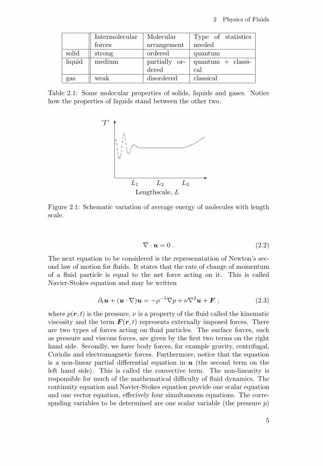
The macroscopic properties of matter (solids, liquids and gases) are directlyrelated to their molecular structure and to the nature of the forces betweenthe molecules. Different molecular properties implies different thermody-namic states. The manner in which some of the molecular properties of aliquid stand between those of a solid and those of a gas is shown in Ta-ble 2.1. Before one can formulate basic equations, certain preliminary ideasare needed. Starting by making the assumtion of the applicability of contin-uum mechanics or the continuum hypothesis. Suppose that we can associatewith any volume of fluid, no matter how small, macroscopic properties, forexample the temperature with that of the fluid in bulk. This assumption isnot correct if we go down to molecular scales, so a fluid particle thus mustbe large enough to contain many molecules. It must still be effectively apoint with respect to the flow as a whole. Thus the continuum hypothesiscan be valid only if there is a length scale, L2, which we can think of asthe size of a fluid particle, such that L1 � L2 � L3 where the meaning ofL1 and L3 is illustrated by Fig. 2.1. When the volume is so small that itcontains only a few molecules and is characterized with a length scale L1,there are large random fluctuations, associated with a Brownian motion.At the other extreme, the volume may become so large that it extends toregions where the temperature is significantly different. So L3 is a typicallength over which the macroscopic properties vary appreciably.

Now to the actual formulation of equations. The fundamental axioms offluid dynamics are the conservation laws. Consider first the representationof mass conservation, often called the continuity equation. This is given by

∂tρ + ∇ · (ρu) = 0 , (2.1)

where ρ(r, t) is the density and u(r, t) is the velocity of the fluid. A fluidproblem is called compressible if the pressure variations in the flow field arelarge enough to effect substantial changes in the density of the fluid. Flows ofliquids with pressure variations much smaller than those required to causephase change (cavitation), or flows of gases involving speeds much lowerthan the isentropic sound speed are termed incompressible. The continuityequation Eq. (2.1) then reduces to

4

2 Physics of Fluids

Intermolecularforces

Moleculararrangement

Type of statisticsneeded

solid strong ordered quantumliquid medium partially or-

deredquantum + classi-cal

gas weak disordered classical

Table 2.1: Some molecular properties of solids, liquids and gases. Noticehow the properties of liquids stand between the other two.

’T ’

Lengthscale, L

L1 L2 L3

�

�

Figure 2.1: Schematic variation of average energy of molecules with lengthscale.

∇ · u = 0 . (2.2)

The next equation to be considered is the represenatation of Newton’s sec-ond law of motion for fluids. It states that the rate of change of momentumof a fluid particle is equal to the net force acting on it. This is calledNavier-Stokes equation and may be written

∂tu + (u · ∇)u = −ρ−1∇p + ν∇2u + F , (2.3)

where p(r, t) is the pressure, ν is a property of the fluid called the kinematicviscosity and the term F (r, t) represents externally imposed forces. Thereare two types of forces acting on fluid particles. The surface forces, suchas pressure and viscous forces, are given by the first two terms on the righthand side. Secondly, we have body forces, for example gravity, centrifugal,Coriolis and electromagnetic forces. Furthermore, notice that the equationis a non-linear partial differential equation in u (the second term on theleft hand side). This is called the convective term. The non-linearity isresponsible for much of the mathematical difficulty of fluid dynamics. Thecontinuity equation and Navier-Stokes equation provide one scalar equationand one vector equation, effecively four simultaneous equations. The corre-spnding variables to be determined are one scalar variable (the pressure p)

5

and one vector variable (the velocity u), effectively four unknown quantities,so in that sense the set of equations is closed.

The kinematic viscosity, ν, is effectively a diffusivity for the velocity u,having the same dimensions [length]× [velocity] like all diffusivities. Valuesof ν and the equivalent dynamic viscosity μ = ν/ρ for some common fluidsat 15◦C and one atmosphere pressure are presented in Table 2.2.

There are several ways to reformulate Eq. (2.3) with the use of vectoridentities. For example, we may write Eq. (2.3) as

∂tu + ω × u +12∇u2 = −ρ−1∇p − ν∇× ω + F , (2.4)

where ω = ∇×u. This appearance of Navier-Stokes equation will be helpfulfor the analysis in Ch. 3.2.

2.2 Reynolds Number

In fluid dynamics, Reynolds number, Re, is an important non-dimensionalnumber and it implies a rough estimation of the relative magnitudes of twokey terms in the equation of motion, Eq. (2.3). which is the ratio

|inertia term||viscous term| =

|(u · ∇)u||ν∇2u| =

O(U2L−1)O(νUL−2)

= O

(UL

ν

)= O(Re) . (2.5)

Stokes flow is a flow at very small Reynolds numbers, such that inertialforces can be neglected compared to viscous forces. Solutions of this prob-lem are reversible in time, i.e. still make sense when reversing the motion.On the contrary, high Reynolds numbers indicate that the inertial forcesare more significant than the viscous (friction) forces. Therefore, we mayassume the flow to be an inviscid flow, an approximation in which we ne-glect the viscosity as compared to the inertial term. The standard equationsof inviscid flow are called the Euler equations. Another often used model,especially in computational fluid dynamics, is to use the Euler equationsfar from the body and the boundary layer equations, which incorporate vis-cosity, close to the body. The Euler equations can be integrated along astreamline to get the well known as Bernoulli’s equation. When the flow iseverywhere irrotational (contains no vorticity, see Ch. 3.1) as well as invis-cid, Bernoulli’s equation can be used throughout the field. A complicationat high Reynolds number is that steady flows are often unstable to smalldisturbances, and may, as a result, become turbulent.

2.3 Boundary Conditions

Since the governing equations of fluid motion are differential equations, thespecification of any problem must include the boundary conditions. Thereare various types of boundaries, but we restrict ourself to the most commontype of boundary to a fluid region, the rigid impermeable wall. One apply-ing condition is obiously the requirement that no fluid should pass through

6

2 Physics of Fluids

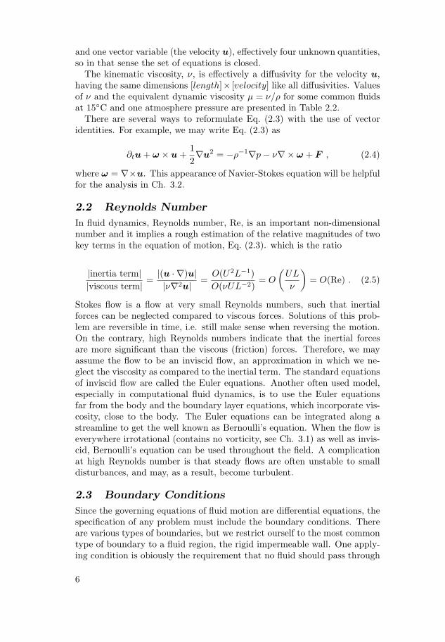
μ [g cm−1 s−1] ν [cm2 s−1]air 0.00018 0.15water 0.011 0.011mercury 0.016 0.0012olive oil 0.99 1.08glycerine 23.3 18.5

Table 2.2: Dynamic viscosity and kinematic viscosity for some commonfluids.

un

fluidsolid

������

��

���

Figure 2.2: Velocity vectors of solid and fluid particles immediately next toits surface.

the wall. The condition on the tangential component of velocity to be zeroat solid boundaries is known as the no-slip or adherence condition, and itholds for a fluid of any viscosity ν �= 0. In the language of partial differ-ential equations the no slip case corresponds to a Dirichlet-type boundarycondition. Summing up, we have the following relations for the velocity offluid, u, at solid boundaries at rest, with a unit normal n to the surface(see Fig. 2.2)

u · n = u × n = 0 . (2.6)

Some remarks about the boundary conditions may be noticed. About twocenturies ago Navier proposed a more general boundary condition that al-lows slip at the surface. The boundary condition states that the tangentialcomponent of the velocity at the surface is proportional to the tangentialstress at the surface. For a flat wall, the boundary condition reduces tovt = λ0∂nvt, where vt is the tangential velocity, ∂nvt is its normal deriva-tive, and λ0 is the slip length. Currently there is a major interest in slipflows in microfluids, where slip lengths heve been measured [42, 41]. Also,there are recent theoretical studies on streamline patterns when the slip-parameter λ0 is changed [43, 44].

In paper II we discuss how the no-slip boundary condition acts as a sourceof vorticity in fluid flows. Then, one needs to add to the right-hand side ofEq. (2.3) the forces acting on the system boundaries. They are of the formof an externally applied pressure at inlets and outlets and viscous stress(vorticity) at solid walls. The velocity field may be calculated explicitlyand shown to depend on boundary conditions only.

7

3 Vorticity

The subject of vorticity and vortices is of general interest in mechanical en-gineering, chemical engineering and also in powder technology. The studiesof vortices also has a respectable history. For example, Leonardo da Vincidepicted very interesting drawings of various kinds of vortex and eddy flows.

Traditionally, fluid motion is described by Navier-Stokes equation, whichis written in terms of the fluid velocity at every point and expresses Newton’slaw that force equals mass times acceleration. In this chapter the voticityequation for determining fluid flow is presented. Then an introduction ofvelocity potentials is made, together with a discussion about simplificationsof the flow equations used in the papers. Further, some examples of vortexmodels is presented. Finally, the 2-D flow around a cylinder is studied anda solution based on method given in Paper II is proposed.

3.1 Concepts and Equations

The vorticity, ω(r, t), of a fluid motion is defined as

ω = ∇× u . (3.1)

This quantity corresponds to rotation of the fluid. Flow without vorticity iscalled irrotational flow. An equation for the vorticity in incompressible flowis obtained by applying the curl operation to the Navier-Stokes equation,Eq. (2.3),

∂tω + (u · ∇)ω = (ω · ∇)u + ν∇2ω . (3.2)

The first term of the right-hand side of Eq. (3.2) represents the action ofvelocity variations on the vorticity. The signifigance of the second term onthe right-hand side is the action of viscosity which produces diffusion ofvorticity. The second term on the left-hand side descibes the convectivetransport of vorticity. The vorticity transport equation may also be castedin the form

∂tω + u × Δu − (∇u −∇ω) (u · ω) = ν∇2ω , (3.3)

where the symbol ∇u indicates that the derivatives are with respect to thecomponents of u only. The vortex motion in 3-D space differs from 2-Din several ways. The most important result is vortex stretching and theconsequent of non-conservation of vorticity. In 2-D flows, the velocity isperpendicular to the vorticity, so u · ω = 0.

When the external force is only the gravitational force, the fluid flowdescribes an irrotational motion. Such a rotational motion is called a freevortex motion or natural vortex motion and the circumferential velocityuθ ∼ 1/r. When one considers the motion of a viscous fluid, the viscositygives the resistance force to the motion of fluid while the external force isthe gravitational force. Indeed, when there is the very high deformation,

8

3 Vorticity

����

����

(a) uθ ∼ 1/r (b) uθ ∼ r

���� � ������

�����

�

�

Figure 3.1: A crude vorticity meter’s behaviour when immersed in a linevortex flow (a) and a uniformly rotating flow (b).

the frictional force becomes very high. Then, if one assumes the fluid tobe a nearly perfect, it is impossible to create the free vortex motion nearthe center of the axis due to the high deformation of the fluid particles.Therefore it is assumed that the center axis rotates as a solid body, uθ ∼ r.

By organizing the two flows in Fig. 3.1 together in the following way

uθ =

{Ωr r < aΩa2

r r > a ,(3.4)

one obtains a so-called Rankine vortex, which serves as a simple model for areal vortex. The circumferential velocity uθ and the vorticity ω for a Rank-ine vortex are shown in Fig. 3.2. Real vortices are typically characterizedby fairly small vortex cores in which the vorticity is concentrated, whileoutside the core the flow is essentially irrotational. The core is not usuallyexactly circular, nor is the vorticity uniform within it.

For an arbitrary closed circuit C in a fluid flow, the circulation Γ is definedas

Γ =∮

C

u · ds . (3.5)

The circulation is related to the vorticity by Stokes theorem∮C

u · ds =∫∫

(∇× u) · dS =∫∫

ω · dS . (3.6)

There must be vorticity within a loop round which circulation occurs. Theexistence of closed streamlines in a flow pattern implies that there are loopsfor which Γ �= 0 and thus that the flow is not irrotational everywhere.However, the converse may not apply.

3.2 Velocity Potentials and Stream Function

If we have the continuity equation of the form in Eq. (2.2) one may applyHelmholtz decomposition [45]. That is, the velocity u may be uniquely

9

(a) (b)

Ωa 2Ω

uθ ω

ra ra

�

�

�

������

Figure 3.2: Distribution of (a) circumferential velocity uθ and (b) vorticityω in a Rankine vortex.

defined by a rotational part urot determined by a vector potential A, anda potential part upot determined by a scalar potential φ as

u = urot + upot = ∇× A + ∇φ . (3.7)

It also follows from the continuity equation, Eq. (2.2), that φ has to satisfythe Laplace equation Δφ = 0, if there are no sources and sinks. The vorticityis determined from the vector potential as ω = ∇(∇·A)−ΔA. It is possibleto choose A such that ∇ · A = 0, a gauge condition.

A particular kind of simple solutions to the flow equation is when thenon-linear terms are explicitly zero due to properties of the solution. Infinding solutions of this kind, one may be guided by the observation thatnon-linear terms disappear from the vorticity equation if:

1. the velocity is parallel to the vorticity, as seen from Eq. (2.4), or

2. the velocity is orthogonal to the vorticity and Δu is parallel to u, asseen from Eq. (3.3).

The vorticity then satisfies the vector Helmholtz equation ∂tω = νΔω. Thisresult has been used in Paper I, III and IV to formulate vortex models. For2-D or axisymmetric flows, only one component of A is non-zero. In thiscase, Eq. (2.2) can always be satisfied by introducing ψ such that

ux = ∂yψ, uy = −∂xψ , (3.8)

where ψ is known as the stream function, since it is constant along a stream-line. The stream function corresponds then to the only non-zero componentof A.

Now, suppose we have that ∇ · A = 0 everywhere, the equation for A isΔA = −ω of which a solution is

10

3 Vorticity

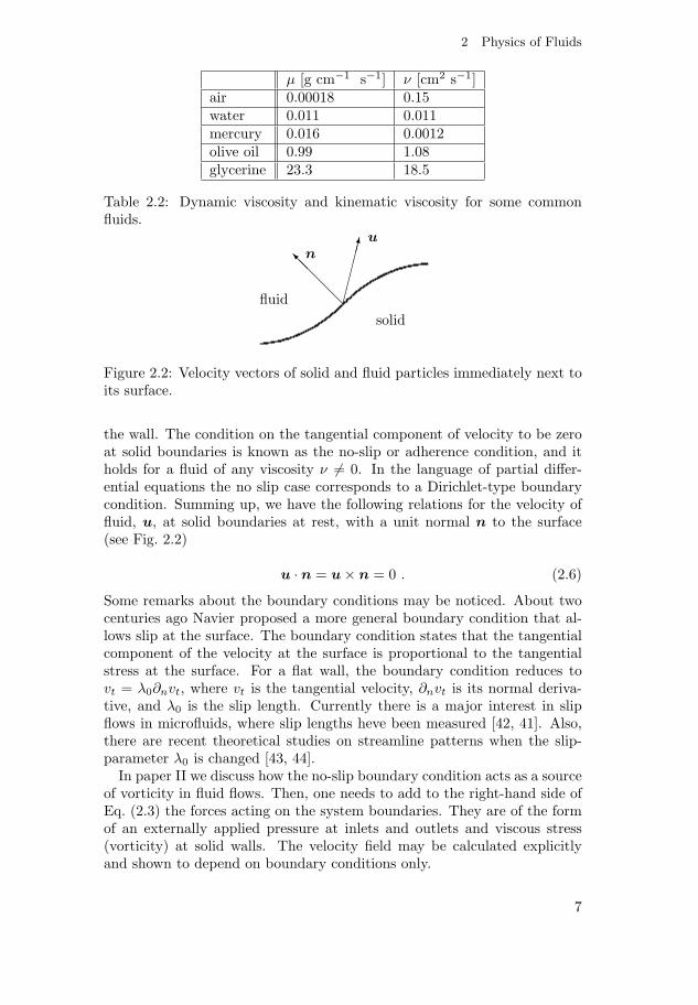
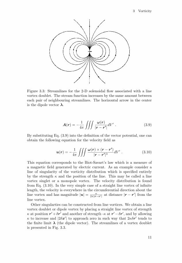
Figure 3.3: Streamlines for the 2-D solenoidal flow associated with a linevortex doublet. The stream function increases by the same amount betweeneach pair of neighbouring streamlines. The horizontal arrow in the centeris the dipole vector λ.

A(r) = − 14π

∫∫∫ω(r)

|r − r′|dV ′ . (3.9)

By substituting Eq. (3.9) into the definition of the vector potential, one canobtain the following equation for the velocity field as

u(r) = − 14π

∫∫∫ω(r) × (r − r′)

|r − r′|3 dV ′ . (3.10)

This equation corresponds to the Biot-Savart’s law which is a measure ofa magnetic field generated by electric current. As an example consider aline of singularity of the vorticity distribution which is specified entirelyby the strength κ and the position of the line. This may be called a linevortex singlet or a monopole vortex. The velocity distribution is foundfrom Eq. (3.10). In the very simple case of a straight line vortex of infinitelength, the velocity is everywhere in the circumferential direction about theline vortex and has magnitude |u| = κ

2π|r−r′| at distance |r − r′| from theline vortex.

Other singularties can be constructed from line vortices. We obtain a linevortex doublet or dipole vortex by placing a straight line vortex of strengthκ at position r′ +δr′ and another of strength -κ at r′−δr′, and by allowingκ to increase and |2δx′| to approach zero in such way that 2κδr′ tends tothe finite limit λ (the dipole vector). The streamlines of a vortex doubletis presented in Fig. 3.3.

11

Figure 3.4: Streamlines in the region r ≤ a for the steady flow due tovorticity proportional to J1(kr) sin θ (r ≤ a, ka = 3.83) and a uniformstream function with suitable chosen speed at infinity.

3.3 Classical Vortex Motions and Models

Here follows a presentation of some models of vortices. A couple of themare of historical interest, others are examples of special cases where simplesolutions may be obtained. There are comments in the examples how torelate them to the present work in the papers.

Lamb-Chaplygin dipole vortex

One of the first nontrivial vortical solution, the translating circular dipole,was suggested independently more then a century ago by Lamb [46] andChaplygin [47]. Since that time, most of the research in the dynamicsof localized distributed vortices has been associated with monopoles anddipoles or their combinations. The Lamb-Chaplygin dipole model assumesa linear relation between vorticity and the stream function ω = k2ψ (withk a constant) within an isolated circular region with radius r = a, and apotential flow ω = 0 in the exterior region (r > a). The solution in terms ofthe stream function of the flow, relative to a comoving frame with velocityU , is

ψ =

{− 2UkJ0(ka)J1(kr) sin θ r < a

U(r − a2

r

)sin θ r > a

, (3.11)

where J0 and J1 are the zero- and first-order Bessel functions, and ka isa root of J1. The latter means that there is a countable spectrum of al-lowed values of ka and, correspondingly, a countable set of interior solutionsmatching the same exterior solution. When the first root of J1 is taken aska, the solution represents a true dipole (see Fig. 3.4).

12

3 Vorticity

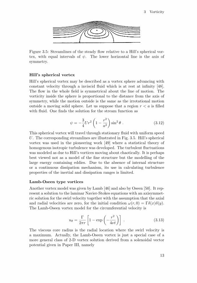
Figure 3.5: Streamlines of the steady flow relative to a Hill’s spherical vor-tex, with equal intervals of ψ. The lower horizontal line is the axis ofsymmetry.

Hill’s spherical vortex

Hill’s spherical vortex may be described as a vortex sphere advancing withconstant velocity through a inviscid fluid which is at rest at infinity [48].The flow in the whole field is symmetrical about the line of motion. Thevorticity inside the sphere is proportional to the distance from the axis ofsymmetry, while the motion outside is the same as the irrotational motionoutside a moving solid sphere. Let us suppose that a region r < a is filledwith fluid. One finds the solution for the stream function as

ψ = −34Ur2

(1 − r2

a2

)sin2 θ . (3.12)

This spherical vortex will travel through stationary fluid with uniform speedU . The corresponding streamlines are illustrated in Fig. 3.5. Hill’s sphericalvortex was used in the pioneering work [49] where a statistical theory ofhomogenous isotropic turbulence was developed. The turbulent fluctuationswas modeled as due to Hill’s vortices moving about chaotically. It is perhapsbest viewed not as a model of the fine structure but the modelling of thelarge energy containing eddies. Due to the absence of internal structureor a continuous dissipation mechanism, its use in calculating turbulenceproperties of the inertial and dissipation ranges is limited.

Lamb-Oseen type vortices

Another vortex model was given by Lamb [46] and also by Oseen [50]. It rep-resent a solution to the laminar Navier-Stokes equations with an axisymmet-ric solution for the swirl velocity together with the assumption that the axialand radial velocities are zero, for the initial condition ω(r, 0) = Γδ(x)δ(y).The Lamb-Oseen vortex model for the circumferential velocity is

uθ =Γ

2πr

[1 − exp

(− r2

4νt

)]. (3.13)

The viscous core radius is the radial location where the swirl velocity isa maximum. Actually, the Lamb-Oseen vortex is just a special case of amore general class of 2-D vortex solution derived from a solenoidal vectorpotential given in Paper III, namely

13

A(r, t) = A(r, θ, t)e =rn cos nθ

(νt)βF

(r√νt

)e , (3.14)

where n is an integer giving the order of the vortex multiplet, e is a unit vec-tor, β is a parameter characterizing the dynamic behaviour, F is a functionof the diffusive variable r√

νt. In [51] another model of Lamb-Oseen type,

originally found by Taylor [52], is used to descibe the decay of monopo-lar vortices in a stratified fluid which was investigated experimentally. Thismodel may also be generated from the general vector potential in Eq. (3.14).

Burgers’ vortex

In 1938 Taylor also recognised the fact that the competition between stretch-ing and viscous diffusion of vorticity must be the mechanism controlling thedissipation of energy in turbulence [53]. A decade later Burgers obtainedexact solutions describing steady vortex tubes and layers in locally uniformstraining flow where the two effects are in balance [54]. Burgers introducedthis vortex as ”a mathematical model illustrating the theory of turbulence”,and he noted particularly that the vortex had the property that the rate ofviscous dissipation per unit length of vortex was independent of viscosity inthe limit of vanishing viscosity (i.e. high Reynolds number). The discoveryof the exact solutions stimulated the development of the models of the dis-sipative scales of turbulence as random collections of vortex tubes and/orsheets. The intermittent nature of the vorticity field was observed in exper-iments by taking statistical measurements which indicated the existence ofthe small-scale localised structures [55].

The exact solution of a 3-D vortex satifying the Navier-Stokes equationgiven by Burgers is in cylindrical coordinates

ur = −αr

2, uθ =

Γ2πr

[1 − exp

(−αr2

4ν

)], uz = αz (3.15)

where α > 0 and Γ are constants. The vorticity is given by

ω =αΓ4πν

exp(−αr2

4ν

)ez (3.16)

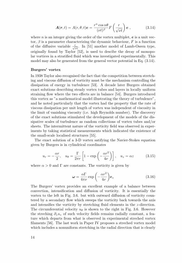
The Burgers’ vortex provides an excellent example of a balance betweenconvection, intensification and diffusion of vorticity. It is essentially thevortex to the left in Fig. 3.6. but with outward diffusion of vorticity coun-tered by a secondary flow which sweeps the vorticity back towards the axisand intensifies the vorticity by stretching fluid elements in the z-direction.The circumferential velocity uθ is shown to the right in Fig. 3.6. Howeverthe streching ∂zuz of such velocity fields remains radially constant, a fea-ture which departs from what is observed in experimental streched vortexfilaments [56]. The last work in Paper IV proposes a streched vortex modelwhich includes a nonuniform stretching in the radial direction that is clearly

14

3 Vorticity

1 2 3 4 5r

0.1

0.2

0.3

0.4

0.5

0.6

Variation of uΘ with r

Figure 3.6: (left) Picture of Burgers’ vortex. (right) The variation of uθ

with r.

present in real flows, as well as the slow variation of velocity profiles alongthe vortex axis.

Vortex ring

The motion of a vortex ring shows interesting phenomena for the physicalprocess for which the fundamental investigation was already established byKelvin, Maxwell and Lamb [57, 58, 46]. A more recent review is given in[59]. Vortex rings can be formed by ejecting a puff of smoke suddenly fromthe mouth through rounded lips and which travels forward steadily with asmoke-filled core. The essential requirement for the production of a vortexring is that linear momentum should be imparted to the fluid with axialsymmetry. One of the observed properties of all vortex rings in uniformfluid is the approximate steadiness of the motion relative to the ring whenthe ring is well clear of the generator and this has been proved for inviscidvortex rings [60]. There is some decay of the motion always, presumablydue to the action of viscosity, but the decay is less for larger rings, suggest-ing that the motion should be truly steady at infinite Reynolds number.In [61], the velocity field inside a viscous vortex ring is obtained on thebasis of an existing solution of the Stokes equation for the velocity in amoving coordinate system (see Fig. 3.7). Their study generated a expres-sion for the velocity in terms of modified Bessel functions and exponentialfunctions which where approximated by polynoms. In Paper IV an exactsolution based on a Greens function for the diffusion equation in sphericalcoordinates is found,

u(r, t) = e−(r2−R2)

4νt (4πνt)−32

[cot θ

rI1

(rR

2νt

)er

+(

r

2νtI1

(rR

2νt

)− R

2νtI0

(rR

2νt

))eθ + 0 eφ

], (3.17)

where I0 and I1 are modified Bessel functions. The solution is compared

15

z

r

R

O

U

�

�

�

���

Figure 3.7: (left) Coordinate system of a cross section of a vortex ring ofradius R propagating with a speed U . (right) Schematic picture of a vortexring.

with very recent experimental observations [62, 63] of the velocity and vor-ticity field, together with the turbulent energy spectrum and they show agood agreement.

A general expression for the propagation velocity U of a viscous vortexring valid for arbitrary vorticity, ω, and stream function distributions, ψ,was found by Saffman [64] (cylindrical coordinates)

U =

∫ ∞0

∫ ∞−∞(ψ + 6zrν)ωdzdr

2∫ ∞0

∫ ∞−∞ r2ωdzdr

(3.18)

In [64] Eq. (3.18) was derived using the Lamb transformation [46] for thevelocity of a ring in an ideal fluid and the validity of its application toa viscous fluid was proved. Continued calculations with the solution inEq. (3.17) may be done for the propagation velocity and compared withexperiments in [65].

Furthermore, the reduction of Navier-Stokes equation to diffusion typeequation, ∂tω = νΔω, may be solved in toroidal coordinates [66]. An exactsolution can be obtanied containing trigonometric and Legendre functionsfor the space varibles. A limitation here is that only an exponential decayin time is possible. Diffusive coordinates can not be used due to a non-separable diffusion equation in toroidal coordinates.

Trailing vortex

The vortices generated at the edge of the wings of an airplane are calledtrailing vortex or the wing tip vortex. The prediction of the induced ve-locities and circulation history of the tip vortices as they trail behind anaircraft has been the subject of much research over the past decades, for areview of see for example [67, 68, 69]. The trailing vortex is generated bythe intrusion of the stream around the wing tip from the high static pres-sure on the lower surface of the wing to the low static pressure on the uppersurface due to the static pressure difference between both surfaces of the

16

3 Vorticity

winglow p

high p

����������������

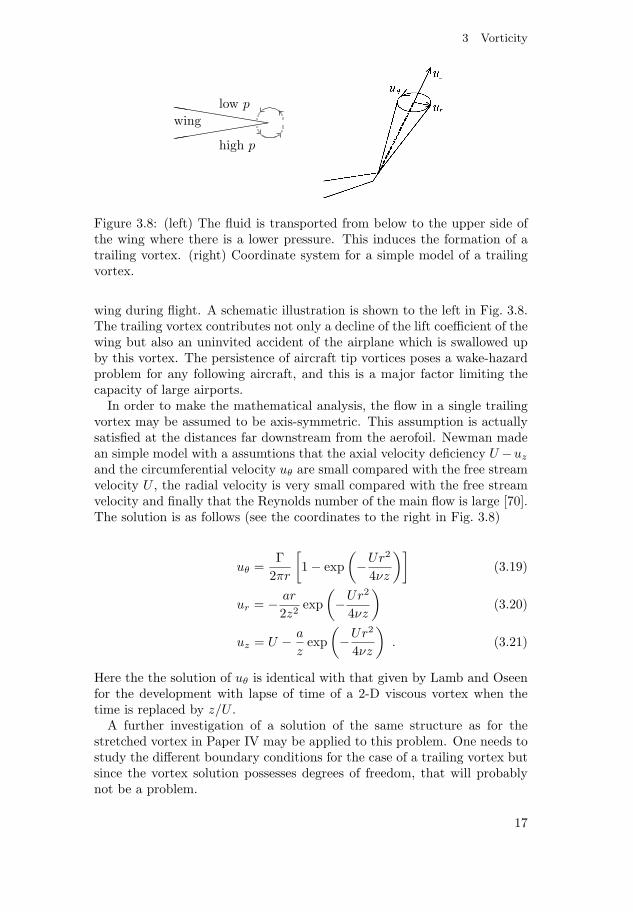
Figure 3.8: (left) The fluid is transported from below to the upper side ofthe wing where there is a lower pressure. This induces the formation of atrailing vortex. (right) Coordinate system for a simple model of a trailingvortex.

wing during flight. A schematic illustration is shown to the left in Fig. 3.8.The trailing vortex contributes not only a decline of the lift coefficient of thewing but also an uninvited accident of the airplane which is swallowed upby this vortex. The persistence of aircraft tip vortices poses a wake-hazardproblem for any following aircraft, and this is a major factor limiting thecapacity of large airports.

In order to make the mathematical analysis, the flow in a single trailingvortex may be assumed to be axis-symmetric. This assumption is actuallysatisfied at the distances far downstream from the aerofoil. Newman madean simple model with a assumtions that the axial velocity deficiency U −uz

and the circumferential velocity uθ are small compared with the free streamvelocity U , the radial velocity is very small compared with the free streamvelocity and finally that the Reynolds number of the main flow is large [70].The solution is as follows (see the coordinates to the right in Fig. 3.8)

uθ =Γ

2πr

[1 − exp

(−Ur2

4νz

)](3.19)

ur = − ar

2z2exp

(−Ur2

4νz

)(3.20)

uz = U − a

zexp

(−Ur2

4νz

). (3.21)

Here the the solution of uθ is identical with that given by Lamb and Oseenfor the development with lapse of time of a 2-D viscous vortex when thetime is replaced by z/U .

A further investigation of a solution of the same structure as for thestretched vortex in Paper IV may be applied to this problem. One needs tostudy the different boundary conditions for the case of a trailing vortex butsince the vortex solution possesses degrees of freedom, that will probablynot be a problem.

17

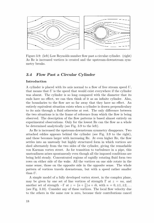
Figure 3.9: (left) Low Reynolds number flow past a circular cylinder. (right)As Re is increased vortices is created and the upstream-downstream sym-metry breaks.

3.4 Flow Past a Circular Cylinder

Introduction

A cylinder is placed with its axis normal to a flow of free stream speed U ,that means that U is the speed that would exist everywhere if the cylinderwas absent. The cylinder is so long compared with the diameter that itsends have no effect, we can then think of it as an infinite cylinder. Also,the boundaries to the flow are so far away that they have no effect. Anentirely equivalent situation exists when a cylinder is drawn perpendicularyto its axis through a fluid otherwise at rest. The only difference betweenthe two situations is in the frame of reference from which the flow is beingobserved. The description of the flow patterns is based almost entirely onexperimental observations. Only for the lowest Re can the flow as a wholebe determined analytically (see Fig. 3.9 to the left).

As Re is increased the upstream-downstream symmetry disappears. Twoattached eddies appears behind the cylinder (see Fig. 3.9 to the right),and these becomes larger with increasing Re. At even higher Re, the flowsettles into an unsteady but highly structured form in which vortices areshed alternately from the two sides of the cylinder, giving the remarkablevon Karman vortex street. As for transition to turbulence in a pipe, thisunsteadiness arises spontaneosly even though all the imposed conditions arebeing held steady. Concentrated regions of rapidly rotating fluid form tworows on either side of the wake. All the vortices on one side rotate in thesame sense, those on the opposite side in the opposite sense. The wholepattern of vortices travels downstream, but with a speed rather smallerthan U .

A simple model of a fully developed vortex street, in the complex plane,may be given by one set of line vortices of strength Γ at z = na, andanother set of strength −Γ at z =

(n + 1

2

)a + ib, with n = 0,±1,±2, . . .

(see Fig. 3.10). Consider any of these vortices. The local flow velocity dueto the others in the same row is zero, because their contributions cancel

18

3 Vorticity

����

b

a

�

�

� � � � �� � � � �

Figure 3.10: Line vortex representation of a Karman vortex street in thewake of a cylinder. Note the relative positions of the vortices.

in pairs. The y-components of velocity due to those in the other row alsocancel in pairs, but the x-components reinforce each other to give a velocityV to the left if Γ > 0. One can show that the whole vortex street moves tothe left with speed V = Γ

2a tanh(

πba

)[39].

Solution by the method given in Paper II

This problem may be analyzed by the techique proposed in Paper II. Westart by considering a velocity field determined by a vector potential A incylindrical coordinates r and θ and time t

A(r, t) =(

r +1r− 2

) ∑n,m

r−n [αn,m(t′) cos mθ + βn,m(t′) sinmθ] δ(t−t′)ez

=∑n,m

r−n+1 [an,m(t′) cos mθ + bn,m(t′) sinmθ] δ(t − t′)ez . (3.22)

The r-dependent factor in front of the sum is included to satisfy the no-slipboundary condition at r = 1. The coefficients α and β are assumed tooscillate slightly around a mean value and the indices n and m run fromzero and upwards. We take m ≤ n, which may be motivated by consideringthe potential as a function of the complex variables z and z∗ and invokingsymmetry arguments. To facilitate the notation and practical calculations,it is convenient to introduce the sets of coefficients a and b that are linearcombinations of the coefficients α and β. These relations are easily derivedfrom Eq. (3.22). The resulting velocity components are

ur =∑n.m

r−nm [−an,m sin mθ + bn,m cos mθ] (3.23)

uθ =∑n.m

r−n(n − 1) [an,m cos mθ + bn,m sin mθ] . (3.24)

19

We start by considering the quasi-static part of the velocity field possessingthe property of an instantaneous adaptation to changing boundary condi-tions and obeying the equation derived from the Navier-Stokes equation

uruθ = −∂r

∫∫G(|r−r′|)dS′·∇uθ−r−1∂θ

∫∫G(|r−r′|)dS′·∇ur , (3.25)

where the first term on the right-hand side vanishes as the derivative in theradial direction of ur is zero on the boundary as seen from the equation ofcontinuity and the fact that the velocity satisfies the no-slip condition. TheGreen’s function G has been defined in Paper II.

We assume that just outside the boundary the vector potential is givenby

A(r, t) =∑m

[fm(r, t′) cos mθ + gm(r, t′) sinmθ] δ(t − t′)ez , (3.26)

so that on the boundary one may write

∂rur =∑m

m [−cm(t′) sinmθ + dm(t′) cos mθ] , (3.27)

giving, after integration, the right-hand side of Eq. (3.24) equal to∑m

r−nm2 [cm(t′) cos mθ + dm(t′) sinmθ] δn−2,m . (3.28)

Calculating the product of the velocity components and identifying withEq. (3.27) gives the equations below, Eq. (3.29) and Eq. (3.30). They areto be interpreted in the following manner. The equations are given for fixedvalues of the indices n and m. Put the index N = n+m+1. The left-handside of the equations contain terms where in each product of two coefficients,one of the coefficients has an index N while the other coefficient has a lowerindex. The right-hand side only contains terms where all coefficients havean index smaller than N . Thus, the Eq. (3.28) constitutes a system ofequations if one includes all equations where n and m take values such thattheir sum equals N − 1. By increasing successively the value of N by 1,may one calculate the value of all coefficient a and b given the coefficients cand d and the coefficients of a and b with the smallest index. For a cylinderexposed to a homogenous cross flow, these coefficients would be a0,1 = 0and b0,1 = −1

n−2∑k=0

[ak,k+1an−k,m+k+1 + bk,k+1bn−k,m+k+1] (n − k − 1)(k + 1) =

−n−2∑n′=0

N−n′∑m′=0

[an′,m′an−n′,m+m′ − bn′,m′bn−n′,m+m′ ] (n − n′ − 1)m′

20

3 Vorticity

−n−2∑n′=0

N−n′∑m′=0

[an′,m′an−n′,m−m′ − bn′,m′bn−n′,m−m′ ] (n − n′ − 1)m′

+(n − 2)2dn−2δm,n−2 , (3.29)

n−2∑k=0

[bk,k+1an−k,m+k+1 + ak,k+1bn−k,m+k+1] (n − k − 1)(k + 1) =

−n−2∑n′=0

N−n′∑m′=0

[bn′,m′an−n′,m+m′ − an′,m′bn−n′,m+m′ ] (n − n′ − 1)m′

−n−2∑n′=0

N−n′∑m′=0

[bn′,m′an−n′,m−m′ − an′,m′bn−n′,m−m′ ] (n − n′ − 1)m′

+(n − 2)2cn−2δm,n−2 . (3.30)

We know turn to the velocity field determined by the equation

v(r, t) =1

Re

∫ t

dt′∂r

∫∫K(|r − r′|, t − t′)dS′ · ∇u(r′, t′) , (3.31)

where the diffusive Green’s function is defined in Paper II. Inserting thevelocity derivative from Eq. (3.27), one obtains after integration over theboundary the velocity field

v(r, t) =1

Re

∫ t

dt′∑m

exp[−Re(r2 + 1)

4(t − t′)

]Im

(Re r

2(t − t′)

)

× [cm(t′) sinmθ − dm(t′) cos mθ] , (3.32)

where Im is a modified Bessel function of index m.It remains to satisfy boundary conditions for this velocity field. This

is achieved by subtracting from the right hand side of Eq. (3.32) an iden-tical expression with r equal to 1. One may study periodic solutions byintroducing the Fourier transformed coefficients

cm(ω) =12π

∫dt exp(iωt)cm(t) , (3.33)

and similarly for the d-coefficient. After integration over time, one obtains

v(r, t) =12π

∫dω exp(iωt)

∑m

[cm(ω) sinmθ − dm(ω) cos mθ

]

21

×[Km

(r Re√2iω

)− Km

(Re√2iω

)]Im

(Re√2iω

), (3.34)

where Km is the other modified Bessel function and one should take thereal part of this expression.

22

4 Turbulence

4 Turbulence

The most common form of fluid flow in nature is of an irregular and chaoticform. This is because in real flows, a number of disturbing sources existwhich interact with the main flow field. An growing instability is normallythe first stage of a sequence of changes in the flow, where the final result isthat the flow becomes turbulent.

In this chapter, a summary of the basics in turbulence theory is given. Itis primary based on classical textbooks such as [71, 72, 73, 74]. The lastsubsection is concerning the topic of coherent structures in turbulence. Thefirst part of Paper IV, and the main of Paper III may be classified as studiesof coherent structures in pipe flow and 2-D turbulence, respectively.

4.1 Concepts and Correlations

No short but complete definition of turbulence seems to be possible. Onecan formulate a brief summary, rather than formal definition. Perhaps thebest description is that turbulence is a state of continuous instability. Eachtime a flow changes as a result of an instability, the ability to predict thedetails of the motion is reduced. When successive instabilities have reducedthe level of predictability so much that it is appropiate to describe a flowstatistically, rather than in every detail, then one says that the flow isturbulent.

In the analysis of turbulence, one usually follows the procedure devisedby Reynolds [75] and divides the velocity into a mean and a fluctuatingpart, Ui + ui. Due to the random behavior of a turbulent field, one has todevise an averaging process to obtain deterministic quantaties from someavailable experimental or theoretical data. Average values can be deter-mined in various ways, time average, space average and ensamble average.For stationary and homogenous processes one expects all three averagingprocedures to lead to the same result. This is known as the ergodic hypoth-esis.

A major and important part of the subject of fluid turbulence is to analyzeand understand the internal structure of the turbulent flow fields. Thisis done in studies of various velocity correlations between points of thefield, and it play an essential role in both theoretical and experimentalstudies of turbulence. To illustrate how they can indicate the scale andstructure of a turbulent motion, consider now typical properties of doublecorrelations. Given the second order probability distribution P (u1, u2), weform the mathematical expectation or average of the product u1u2 as

u1u2 =∫ ∞

−∞

∫ ∞

−∞u1u2P (u1, u2)du1du2 , (4.1)

which is called the double correlation. When u1 and u2 are velocities atdifferent positions but at the same instant, u1u2 is known as a space corre-lation. Most attention is usually given to longitudinal and lateral correla-

23

(a) (b)

r

u1

u2

�

�

�

�r

u1

u2

���

���

�

� �

�1

(c)

AB

r

R

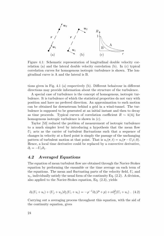
Figure 4.1: Schematic representation of longitudinal double velocity cor-relation (a) and the lateral double velocity correlation (b). In (c) typicalcorrelation curves for homogenous isotropic turbulence is shown. The lon-gitudinal curve is A and the lateral is B.

tions given in Fig. 4.1 (a) respectively (b). Different behaivour in differentdirections may provide information about the structure of the turbulence.

A special case of turbulence is the concept of homogenous, isotropic tur-bulence. It is turbulence of which the statistical properties do not vary withposition and have no prefered direction. An approximation to such motioncan be obtained far downstream behind a grid in a wind-tunnel. The tur-bulence is supposed to be generated at an initial instant and then to decayas time proceeds. Typical curves of correlation coefficient R ∼ u1u2 forhomogenous isotropic turbulence is shown in (c).

Taylor [53] reduced the problem of measurement of isotropic turbulenceto a much simpler level by introducing a hypothesis that the mean flowU1 acts as the carrier of turbulent fluctuations such that a sequence ofchanges in velocity at a fixed point is simply the passage of the unchangingpattern of turbulent motion at that point. That is ui(r, t) = ui(r −U1t, 0).Hence, a local time derivative could be replaced by a convective derivative,∂t = −U1∂1.

4.2 Averaged Equations

The equation of mean turbulent flow are obtained through the Navier-Stokesequation by preforming the ensamble or the time average on each term ofthe equations. The mean and fluctuating parts of the velocity field, Ui andui, individually satisfy the usual form of the continuity Eq. (2.2). A division,also applied to the Navier-Stokes equation, Eq. (2.3), yields

∂t(Ui + ui) + (Uj + uj)∂j(Ui + ui) = −ρ−1∂i(P + p) + ν∂2j (Ui + ui) . (4.2)

Carrying out a averaging process throughout this equation, with the aid ofthe continuity equation, gives

24

4 Turbulence

y

x

−u

v�

�

�

�

�

���

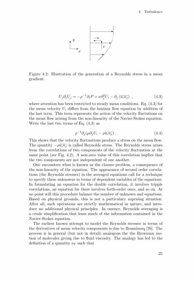
Figure 4.2: Illustration of the generation of a Reynolds stress in a meangradient.

Uj∂jUj = −ρ−1∂iP + ν∂2j Ui − ∂j (uiuj) , (4.3)

where attention has been restricted to steady mean conditions. Eq. (4.3) forthe mean velocity Ui differs from the laminar flow equation by addition ofthe last term. This term represents the action of the velocity fluctutions onthe mean flow arising from the non-linearity of the Navier-Stokes equation.Write the last two terms of Eq. (4.3) as

ρ−1∂j(μ∂jUi − ρuiuj) . (4.4)

This shows that the velocity fluctuations produce a stress on the mean flow.The quantity −ρuiuj is called Reynolds stress. The Reynolds stress arisesfrom the correlations of two components of the velocity fluctuation at thesame point (see Fig. 4.2). A non-zero value of this correlation implies thatthe two components are not independent of one another.

One encounters what is known as the closure problem, a consequence ofthe non-linearity of the equation. The appearance of second order correla-tions (the Reynolds stresses) in the averaged equations call for a techniqueto specify these unknowns in terms of dependent variables of the equations.In formulating an equation for the double correlation, it involves tripplecorrelations, an equation for these involves forth-order ones, and so on. Atno point will this procedure balance the number of unknown and equations.Based on physical grounds, this is not a particulary suprising situation.After all, such operations are strictly mathematical in nature, and intro-duce no additional physical principles. In essence, Reynolds averaging isa crude simplification that loses much of the information contained in theNavier-Stokes equation.

The earliest known attempt to model the Reynolds stresses in terms ofthe derivatives of mean velocity components is due to Boussinesq [76]. Theprocess is in general (but not in detail) analogous the the Brownian mo-tion of molecules giving rise to fluid viscosity. The analogy has led to thedefinition of a quantity νT such that

25

uiuj = νT ∂jUi . (4.5)

νT is called the eddy or turbulent viscosity. It is important to realize thatνT is a representation of the action of the turbulence on the mean flow andnot a property of the fluid. In recent times the intensive area of turbulencemodeling is to devise approximations for the unknown correlations in termsof flow properties that are known, such that a sufficient number of equationsexist. In making such approximations, the system of equations is closed.

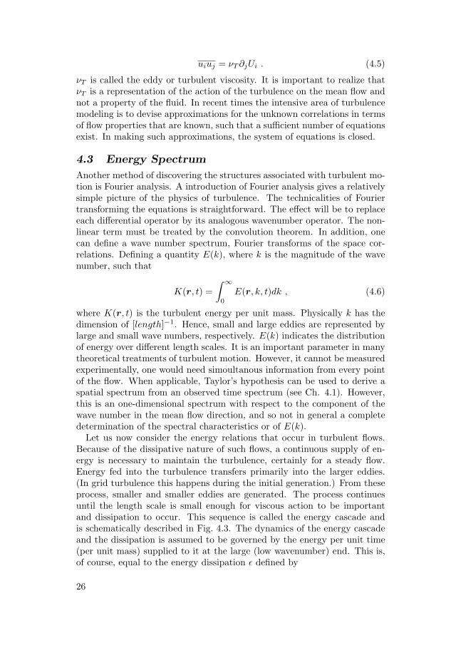
4.3 Energy Spectrum

Another method of discovering the structures associated with turbulent mo-tion is Fourier analysis. A introduction of Fourier analysis gives a relativelysimple picture of the physics of turbulence. The technicalities of Fouriertransforming the equations is straightforward. The effect will be to replaceeach differential operator by its analogous wavenumber operator. The non-linear term must be treated by the convolution theorem. In addition, onecan define a wave number spectrum, Fourier transforms of the space cor-relations. Defining a quantity E(k), where k is the magnitude of the wavenumber, such that

K(r, t) =∫ ∞

0

E(r, k, t)dk , (4.6)

where K(r, t) is the turbulent energy per unit mass. Physically k has thedimension of [length]−1. Hence, small and large eddies are represented bylarge and small wave numbers, respectively. E(k) indicates the distributionof energy over different length scales. It is an important parameter in manytheoretical treatments of turbulent motion. However, it cannot be measuredexperimentally, one would need simoultanous information from every pointof the flow. When applicable, Taylor’s hypothesis can be used to derive aspatial spectrum from an observed time spectrum (see Ch. 4.1). However,this is an one-dimensional spectrum with respect to the component of thewave number in the mean flow direction, and so not in general a completedetermination of the spectral characteristics or of E(k).

Let us now consider the energy relations that occur in turbulent flows.Because of the dissipative nature of such flows, a continuous supply of en-ergy is necessary to maintain the turbulence, certainly for a steady flow.Energy fed into the turbulence transfers primarily into the larger eddies.(In grid turbulence this happens during the initial generation.) From theseprocess, smaller and smaller eddies are generated. The process continuesuntil the length scale is small enough for viscous action to be importantand dissipation to occur. This sequence is called the energy cascade andis schematically described in Fig. 4.3. The dynamics of the energy cascadeand the dissipation is assumed to be governed by the energy per unit time(per unit mass) supplied to it at the large (low wavenumber) end. This is,of course, equal to the energy dissipation ε defined by

26

4 Turbulence

Injectionof energy

Flux ofenergy

Dissipationof energy

����

����

����

��

��

��

��

��

� � � � � � � � � �����

Figure 4.3: Schematic figure of the energy cascade which goes from largerto smaller eddies.

ε = −dK

dt. (4.7)

This suggests that the spectrum function E is independent of the energyproduction processes for all wavenumbers large compared with those atwhich the production occurs. Then E depends only on the wavenumber,the dissipation, and the viscosity, E(k, ε, ν). If the cascade is long enough,there may be an intermediate range in which the action of viscosity hasnot yet occured, that is, E = E(k, ε). Dimensional analysis then givesE = Aε

23 k− 5

3 , where A is a numerical constant. This is a famous result,known as the Kolmogorov − 5

3 law [77].

4.4 Coherent Structures

In recent years it has been increasingly evident that turbulent flows are notjust random or chaotic but can contain more deterministic features, knownas coherent structures. We are now considering some discernible patternsin the flow, which may have random features but nevertheless occur withsufficient regularity, in space or time, to be recognizable as quasi-periodic ornear-deterministic. Quite a variety of structures has been identified, suchas vortices, waves, streaks etc. Here our task is vortex modeling of fullydeveloped turbulence in 2-D and developed structures in pipe flows.

An example of the later one, the visualization of turbulent flows andboundary layers via sophisticated experimental methods like particle imag-ing velocimetry has led to the indentification of a rich variety of prominentcoherent structures [78, 79, 80, 81]. Recently, experimental studies of transi-tional pipe flow has shown the existence of coherent flow structures that aredominated by downstream vortices [19, 20]. Downstream vortices transportliquid across the mean shear gradient and create regions of fast or slow mov-

27

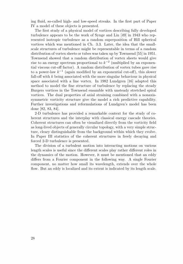
ing fluid, so-called high- and low-speed streaks. In the first part of PaperIV a model of these objects is presented.

The first study of a physical model of vortices describing fully developedturbulence appears to be the work of Synge and Lin [49] in 1943 who rep-resented isotropic turbulence as a random superposition of Hill sphericalvortices which was mentioned in Ch. 3.3. Later, the idea that the small-scale structures of turbulence might be representable in terms of a randomdistribution of vortex sheets or tubes was taken up by Townsend [55] in 1951.Townsend showed that a random distribution of vortex sheets would giverise to an energy spectrum proportional to k−2 (multiplied by an exponen-tial viscous cut-off factor). A random distribution of vortex tubes gave riseto a power-law k−1 (again modified by an exponential cut-off), this slowerfall-off with k being associated with the more singular behaviour in physicalspace associated with a line vortex. In 1982 Lundgren [16] adapted thismethod to model the fine structure of turbulence by replacing the steadyBurgers vortices in the Townsend ensamble with unsteady stretched spiralvortices. The dual properties of axial straining combined with a nonaxis-symmetric vorticity structure give the model a rich predictive capability.Further investigations and reformulations of Lundgren’s model has beendone [82, 83, 84].

2-D turbulence has provided a remarkable context for the study of co-herent structures and the interplay with classical energy cascade theories.Coherent structures can often be visualized directly from the vorticity fieldas long-lived objects of generally circular topology, with a very simple struc-ture, cleary distinguishable from the background within which they evolve.In Paper III statistics of the coherent structures in freely decaying andforced 2-D turbulence is presented.

The division of a turbulent motion into interacting motions on variouslength scales is useful since the different scales play rather different roles inthe dynamics of the motion. However, it must be mentioned that an eddydiffers from a Fourier component in the following way. A single Fouriercomponent, no matter how small its wavelength, extends over the wholeflow. But an eddy is localized and its extent is indicated by its length scale.

28

5 Summary of Papers

5 Summary of Papers

A short summary of each paper included in the second part of this thesis ispresented below. They all concern vortex motions and vortex solutions tothe Navier-Stokes equation.

5.1 Paper I

During cornering winds at buildings, dual conical vortices form in the sep-areted flow along the leading edges of flat roofs. These vortices cause themost extreme wind suction forces found anywhere on the building, so it isimportant to predict them accurately. Therefore, in this paper a model of aconical vortex is proposed. The first experimental and modeling of conicalvortices where related to wing-tip, or trailing, vortices [85, 86] (see Ch 3.3for trailing vortices). Theoretical considerations of vortices attached to flatroofs has mostly been of semi-analytical or hueristic nature [87, 88, 89].

The derivation here is made in spherical coordinates. Assumptions madein the calculations are that the vortex possess a perfect rotational symmetry(no φ-dependence) and that the impact flow is uniform (no atmosphericboundary layer) and quasi-stationary. In the model, the vorticity is parallelto the velocity so the flow equation is reduced to a diffusion type of equationcontaining no non-linear terms. The radial parametrization of the flowfield contains a spherical Bessel function with index l as a free parameter.The θ-dependece of velocity field is represented by a linear combination ofLegendre functions of the first and second kind. By this choise, the boundarycondition of the radial velocity at the edge of the cone, ur(θ = θ0) = 0, canbe fulfilled. The other boundary values for the velocities on the surface ofthe cone, uθ and uφ, are calculated from simple boundary layer theory.

In the model for the flow field there is no implicit dependence on theReynolds number. However, there is still a Re-dependence from the bound-ary conditions. With the velocity determined, the pressure on the boundaryof the cone may be derived by an integration of Navier-Stokes equation, giv-ing Bernoulli equation. Comparison with pressure measurements show goodagreement.

5.2 Paper II

This paper is a mathematical and theoretical study of the Navier-Stokesequation. A solution to the Navier-Stokes equation for internal flow systemsis proposed by considering the vorticity generated at the boundaries of thesystem. There are experimental evidence for the major impact the no-slip boundary conditions has on the whole flow considered [90]. The solidboundaries act as a source of vorticity, which spread into the flow domain.

The Navier-Stokes equation describes the flow in a free space, but itcontains no information how to take into account boundary conditions. Theforces acting on boundaries of the flow domain that have to be included inthe equation are: pressure applied at inlets and outlets and viscous forces

29

at solid boundaries. Then Navier-Stokes can be rewritten in the form ofa divergence and integrated. The resulting equation may be split into twoequations: its symmetric and skew-symmetric part. Further, the diagonalelements of the symmetric equation gives a relation from which the pressuremay be calculated in the flow. The off-diagonal elements of the symmetricequation gain a non-linear but purely algebraic equation for the velocitycomponents.

Now, continued studies of the skew-symmetric equation show it is a lineardifferential equation for a vector potential A. A solution consisting of anintegral kernal similar to such used for the diffusion may be applied. Thisdescribes vorticity generated at solid boundaries as well as contained in fluidleaving or entering the system. Still left undetermined are boundary valuesof the velocity and its gradients (vorticity).

The final part of the paper presents a suggestion about inquiring informa-tion about the velocity and velocity gradients (vorticity) at the boundaries.By the use of the equation of continuity a velocity field vQ from sourcesand sinks in a infinte space is obtained. Then, vQ has to be modified suchthat it satisfies the normal and tangential boundary conditions. This givestwo surface integrals (one from the normal and one from the tangentialcondition) with specified kernals that will be subtracted from infinte spacevelocity vQ.

5.3 Paper III

In Paper III the vortex evolution and connection to turbulence in 2-D flows isdescribed. There exist two common methods to generate 2-D vortical flows,namely in soap films and in stratified systems. See [91, 92] for a rewiew. Thestatified flow is generated in a plastic cell under which permanent magnetsare located, orientated such that to have a vertical magnetization axis. Thecell is filled with two layers of a solution which has different densities. Theheavier solution is on the bottom and the density difference of the interfaceacts to prevent vertical velocities, and thus a bidimensionalization of theflow. The magnets are placed to create a 8×8 array of vortices wiht nearestneighbors counter-rotating.

We have used vortex solutions derived from a solenodial vector potentialA. The vector potential is characterized by three parameters, n the or-der of vortex multiplet, the dynamic behaivor β and j which is the lowersummation index of a sum over a diffusive variable r√

νt. Evolution of the

vorticity fields are calculated and statistics for average vortex radius andnumber of vortices are compared with messurements [27]. Vortex singletsdo not contribute to the energy spectrum so dipoles are used to comparewith the measured turbulent energy spectrum in [28].

Now we turn to the situation of soap films. Two vertical combs areplaced along the channel walls. The teeth of the vertical combs perpetuallygenerate small vortices, which then are quickly swept into the center ofthe channel by larger vortices. A forced, steady turbulent state is created.

30

5 Summary of Papers

We model the flow by a combination of vortex doublets of the same typeas in the stratified layer case, and a stationary part assumed to consist ofa uniform flow. The no-slip boundary condition at the channel walls issatisfied by this choise of combination.

The main results we obtain for the energy spectral function E(k) is thatit scales with k

√νt and that it has an amplitude that is proportional to

νt. Also, we display that E(k) scales as k−3. These results are in goodagreement with experimental results of soap films shown in [34].

5.4 Paper IV

In Paper IV the focus is on vortex structures in 3-D. We give three examplesof recent experimental observations where we find solutions that reproducesthe measurements. First, travelling vortex structures experimentally ob-served in a pipe flow at Re close to transition from laminar to turbulentflow is considered [19, 20]. These vortex structures has stremwise orienta-tion creating local anomalies in the streamwise velocity, called streaks. Theflow in the spanwise direction is weaker but may still be critical for the flowpattern. Our solutions, which are found in spherical coordinates, possessesthe property that the velocity and vorticity are parallell so they are exactsolutions to the non-linear vorticity transport equation. A superposition ofsuch vortices, which still is a exact solution, describes flow patterns observedin [19, 20].

Secondly, vortex rings are studied. New experimental observations madein water are reported in [62, 63]. The vortex rings are generated by pushingwater through the cylindrical nozzle of a pipe submerged in an aquarium. Bythe use of planar laser induced flourescence and particle image velocimetry,the velocity and vorticity profiles together with the energy spectral func-tion for the vortex structure are obtained. We model the vortex ring byelementary vortices with diffusive properties, again in sperical coordinates,where the flow field has the property that the velocity is perpendicular tothe vorticity. Elementary vortices are placed around a circle and integratedto obtain the total flow.

Finally, a stretched vortex experimentally obtained in a water channel[56, 93] is modelled. A small bump on the bottom wall of the channelinduces the initial boundary vorticity to roll up in a vortex. Then thevortex is strongly enhanced by stretching which is produced by suckingthe flow through a hole on each lateral wall. We model the vortex by anelementary vortex structure where the vorticity and velocity is parallel asfor the travelling vortex in a pipe. A distribution of elementary vortices areplaced along the stretching axis and we are able to satisfy the boundaryconditions. The resulting velocity field reproduces the experimental datawith good agreement [56, 93].

31

6 Acknowledgements

First of all I will thank my supervisor, docent Mats D. Lyberg, for bringingme into the interesting field of fluids. I will also thank him for all thesupport and encouragement during the years of the work. Secondly, I willthank everyone at the Physics Department at Vaxjo University for the niceenviroment to work in. Finally, I will thank my family, especially Helena,for all your support.

32

Bibliography

Bibliography

[1] G.A. Tokaty, A History and Philosophy of Fluid Mechanics, Dover Pub-lications, New York, (1971).

[2] D. Gottlieb and S.A. Orszag, Numerical Analysis of Spectral Methods:Theory and Applications, SIAM, Philadelphia, (1977).

[3] G.D. Smith, Numerical Solution of Partial Differential Equations: Fi-nite Difference Methods, 3rd ed., Clarendon Press, Oxford, (1985).

[4] O.C. Zienkiewicz and R.L. Taylor, The Finite Element Method – Vol. 2:Solid and Fluid Mechanics, McGraw-Hill, New York, (1991).

[5] P.G. Saffman, Vortex Dynamics, Cambridge University Press, Cam-bridge, (1992).

[6] A. Ogawa, Vortex Flow, CRC Press, Boca Ranton, Florida, (1993).

[7] J.Z. Wu, H.Y. Ma and M.D. Zhou, Vorticity and Vortex Dynamics,Springer-Verlag, Heidelberg, (2006).

[8] O. Reynolds, Philos. Trans. 174, 935 (1883).

[9] P.G. Drazin and W.H. Ried, Hydrodynamic Stability, Cambridge Uni-versity Press, Cambridge, (1981).

[10] S. Chandrasekhar, Hydrodynamic and Hydromagnetic Stability, DoverPublications, New York, (1981).

[11] P.J. Schmid and D.S. Henningson, Stability and Transition in ShearFlows, Springer-Verlag, New York, (2001).

[12] E.D. Siggia, J. Fluid Mech. 107, 37 (1981).

[13] A. Vincent and M. Meneguzzi, J. Fluid Mech. 225, 1 (1991).

[14] O. Cadot, D. Douady and Y. Couder, Phys. Fluids 7, 630 (1995).

[15] Y. Cuypers, A. Maurel and P. Petitjeans, Phys. Rev. Lett. 91, 1945(2003).

[16] T.S. Lundgren, Phys. Fluids 25, 2193 (1982).

[17] J.C. Vassilicos and J.G. Brasseur, Phys. Rev. E 54, 467 (1996).

[18] B. Hof, A. Juel and T. Mullin, Phys. Rev. Lett. 91, 2445 (2003).

[19] B. Hof, C.W.H. van Doorne, J. Westerweel, F.T.M. Nieuwstadt, H.Faisst, B. Eckhardt, H. Wedin, R. R. Kerswell and F. Waleffe, Science305, 1594 (2004).

33

Bibliography

[20] B. Hof, C.W.H. van Doorne, J. Westerweel and T.M. Nieuwstadt, Phys.Rev. Lett. 95, 2145 (2005).

[21] H. Faisst and B. Eckhardt, Phys. Rev. Lett. 91, 2245 (2003).

[22] F. Waleffe, Phys. Fluids 15, 1517 (2003).

[23] H. Wedin and R. Kerswell, J. Fluid Mech. 508, 333 (2004).

[24] J. Sommeria, J. Fluid Mech. 170, 139 (1986).

[25] O. Cardoso, D. Marteau and P. Tabeling, Phys. Rev. E 49, 454 (1994).

[26] J. Paret and P. Tabeling, Phys. Rev. Lett. 79, 4162 (1997).

[27] A.E. Hansen, D. Marteau and P. Tabeling, Phys. Rev. E 58, 7261(1998).

[28] J. Paret, M-C. Jullien and P. Tabeling, Phys. Rev. Lett. 83, 3418(1999).

[29] Y. Couder, J. Physique Lett. 42, 429 (1981).

[30] Y. Couder, J. Physique Lett. 45, 353 (1984).

[31] H. Kellay, X.L. Wu and W.I. Goldburg, Phys. Rev. Lett. 74, 3975(1995).

[32] X.L. Wu, B. Martin, H. Kellay and W.I. Goldburg, Phys. Rev. Lett.75, 236 (1995).

[33] B. Martin, X.L. Wu, W.I. Goldburg and M.A. Rutgers, Phys. Rev. Lett80, 3964 (1998).

[34] M.A. Rutgers, Phys. Rev. Lett. 81, 2244 (1998).

[35] H. Kellay, X.L. Wu and W.I. Goldburg, Phys. Rev. Lett. 80, 277 (1998).

[36] G.K. Batchelor, An Introduction to Fluid Dynamics, Cambridge Uni-versity Press, Cambridge, (1967).

[37] D.J. Tritton, Physical Fluid Dynamics, Oxford University Press, Ox-ford, (1988).

[38] Z.U.A. Warsi, Fluid Dynamics, Theoretical and Computational Ap-proaches, 2nd ed., CRC Press, Boca Ranton, (1999).

[39] D.J. Acheson, Elementary Fluid Dynamics, Oxford University Press,Oxford, (1990).

[40] L.D. Landau and E.M. Lifshitz, Fluid Mechanics, 2nd ed., PergamonPress, Oxford, (1987).

34

Bibliography

[41] C.-H. Choi, J.A. Westin and K.S. Breuer, Phys. Fluids 15, 2897 (2003).

[42] E. Lauga and H.A. Stone, J. Fluid Mech. 489, 55 (2003).

[43] L. Tophøj, S. Møller and M. Brøns, Phys. Fluids 18, 3102 (2006).

[44] M. Brøns, Adv. Appl. Mech. 41, 38 (2006).

[45] G. Dassios and I.V. Lindell, J. Phys. A 35, 5139 (2002).

[46] H. Lamb, Hydrodynamics, 6th ed., Cambridge University Press, Cam-bridge, (1932).

[47] S.A. Chaplygin, Trans. Phys. Sect. Imperial Moscow Soc. Friends ofNatural Sci. 11, 11 (1903).

[48] M.J.M. Hill, Proc. of the Roy. Soc. of London 55, 219 (1894).

[49] J.L. Synge and C.C. Lin, Trans. R. Soc. Can. 37, 45 (1943).

[50] C.W. Oseen, Ark. J. Mat. Astrom. Fys. 7, 14 (1912).

[51] R.R. Trieling and G.J.F. van Heijst, Fluid Dyn. Research 23, 27 (1998).

[52] G.I Taylor, Reports and Memoranda 598, 73 (1918).

[53] G.I Taylor, Proc. R. Soc. London A 164, 476 (1938).

[54] J.M. Burgers, Adv. Appl. Mech. 1, 197 (1948).

[55] A.A. Townsend, Proc. R. Soc. A 208, 534 (1951).

[56] P. Petitjeans, J.H. Robres, J.E. Wesfreid and N. Kevlahan, Euro. J.Mech. B. /Fluids 17, 549 (1998).

[57] Lord Kelvin, Trans. R. Soc. Edinb. 25, 217 (1869).

[58] J.C. Maxwell, A Treatise on Electricity and Magnetism – Vol. 2, 3rded., Dover Publications, New York, (1954).

[59] K. Shariff and A. Leonard, Annu. Rev. Fluid Mech. 24, 235 (1992).

[60] L.E. Fraenkel, Proc. R. Soc. Lond. A 316, 29 (1970).

[61] F.B. Kaplanskii and Y.A. Rudi, Fluid Dynamics 36, 16 (2001).

[62] A. Dazin, P. Dupont and M. Stanislas, Exp. in Fluids 40, 383 (2006).

[63] A. Dazin, P. Dupont and M. Stanislas, Exp. in Fluids 41, 401 (2006).

[64] P.G. Saffman, Stud. Appl. Math. 49, 371 (1970).

[65] A.H.M. Eisenga, R. Vericco and G.J.F. van Heijst, J. Fluid Mech. 354,69 (1998).

35

Bibliography

[66] H. Tryggeson and M.D. Lyberg, in preparation.

[67] S. E. Widnall, Annu. Rev. Fluid Mech. 7, 141 (1975).

[68] P. R. Spalart, Annu. Rev. Fluid Mech. 30, 107 (1998).

[69] L. Jacquin, Int. J. Heat and Fluid Flow 26, 843 (2005).

[70] B.G. Newman, Aeronaut. Q. 1, 167 (1959).

[71] G.K. Batchelor, The Theory of Homogenous Turbulence, CambridgeUniversity Press, Cambridge, (1982).

[72] J.O. Hinze, Turbulence, McGraw-Hill, New York, (1975).

[73] W.D. McComb, The Physics of Fluid Turbulence, Oxford UniversityPress, Oxford, (1991).

[74] U. Frisch, Turbulence: The Legacy of A.N. Kolmogorov, CambridgeUniversity Press, Cambridge, (1995).

[75] O. Reynolds, Phil. Trans. R. Soc. A 186, 123 (1895).

[76] J. Boussinesq, Mem. pres. par div. savant a l’acad. sci. Paris 23, 46(1877).

[77] A.N. Kolmogorov, Dokl. Akad. Nauk S.S.S.R. 32, 19 (1941).

[78] S. Robinson, Annu. Rev. Fluid Mech. 23, 601 (1991).

[79] P. Holmes, J.L. Lumley and G. Berkooz, Turbulence, Coherent Struc-tures, Dynamical Systems and Symmetry, Cambridge University Press,Cambridge, (1998).

[80] B. Podvin and J. Lumley, J. Fluid Mech. 362, 121 (1998).

[81] R. Panton, Prog. Aerospace Sci. 37, 341 (2001).

[82] D.I. Pullin and P.G. Saffman, Phys. Fluids 5, 126 (1993).

[83] D.I. Pullin, J.D. Buntine and P.G. Saffman, Phys. Fluids 6, 3010(1994).

[84] D.I. Pullin and P.G. Saffman, Annu. Rev. Fluid Mech. 30, 31 (1998).

[85] N.C. Lambourne and D.W. Bryer, Aero. Res. Coun., Dokument 477,(1959).

[86] M.G. Hall, J. of Fluid Mech. 11, 209 (1961).

[87] H. Kawai and G. Nishimura, J. Wind Eng. Ind. Aero. 60, 211 (1996).

[88] C.W. Williams and C.J. Baker, J. Fluids and Structures 11, 767 (1997).

36

Bibliography

[89] D. Banks and R.N. Meroney, Wind and Structures 4, 227 (2001).

[90] G.J.F. van Heijst, H.J.H. Clercx and D. Molenar, J. Fluid Mech. 554,411 (2006).

[91] H. Kellay and W. I. Goldburg, Rep. on Progr. in Phys. 65, 845 (2002).

[92] P. Tabeling, Phys. Rep. 362, 1 (2002).

[93] M. Rossi, F. Bottausci, A. Maurel and P. Petitjeans, Phys. Rev. Lett.92, (2004).

37

I

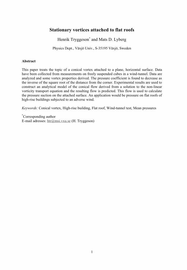
1

Stationary vortices attached to flat roofs

Henrik Tryggeson* and Mats D. Lyberg

Physics Dept., Växjö Univ., S-35195 Växjö, Sweden

Abstract

This paper treats the topic of a conical vortex attached to a plane, horizontal surface. Datahave been collected from measurements on freely suspended cubes in a wind-tunnel. Data areanalyzed and some vortex properties derived. The pressure coefficient is found to decrease asthe inverse of the square root of the distance from the corner. Experimental results are used toconstruct an analytical model of the conical flow derived from a solution to the non-linearvorticity transport equation and the resulting flow is predicted. This flow is used to calculatethe pressure suction on the attached surface. An application would be pressure on flat roofs ofhigh-rise buildings subjected to an adverse wind.

Keywords: Conical vortex, High-rise building, Flat roof, Wind-tunnel test, Mean pressures

*Corresponding authorE-mail adresses: htr@msi.vxu.se (H. Tryggeson)

2

1 Introduction

This paper contains measurements on and a mathematical model of conical vortices adjacentto flat surfaces. The first thorough experimental studies and modeling of conical vortices wererelated to wing tip vortices (Lambourne and Bryer, 1959; Hall, 1961). This was somewhatlater followed by studies of conical vortices attached to walls (Davenport, 1960; Leufheusser,1965) and has seen a continuous development of more refined experiments and theoreticalmodels (Simiu, 1978; Wirén, 1970, 1985, 1990; Lee and Evans, 1984; Kind, 1986; Kramerand Gerhardt, 1991; Doligalski et al, 1994; Tieleman et al, 1996) and, in recent years, by alarge number of studies (for example, Banks and Meroney, 2001; Kawai, 1997; Lin et al,1995; Bienkiewicz and Ham, 2003; Wu et al, 2001) .

Below follows a brief overview of the main physical and mathematical background of thetopic treated. Some experimental results of the main problem are presented in Sections 2 and3. In Section 4 appears the derivation of the mathematical model applied. Section 5 treats theconnection between model and what results are to be expected from theory for wall boundarylayers rolling up into a vortex. Section 6 contains results and a discussion.

The main aim of this paper is to find a simple description of a conical vortex attached to aplanar horizontal surface. The velocity field will be the desired output, from which thepressure may be determined. The input is measured data of the incoming flow, which willserve as boundary conditions to solutions of the differential equations governing a flow.

Suppose we have an incompressible newtonian fluid. The Navier-Stokes equation and theequation of continuity govern its motion. These equations contain all the dynamic informationabout a fluid in motion. We will use spherical co-ordinates applied to a cone with the z-axis ofthe co-ordinate system along the principal axis.

A conical vortex appears, for example, close to the edge at the roof of buildings, as in Fig. 1.The airflow released from the vertical side rolls up into two conical vortices (Kramer andGerhardt, 1991; Banks et al, 2000; Banks and Meroney, 2001; Wu et al, 2001), as isschematically indicated in Fig. 2. The presence of the cones bring about suction on the roofbelow the vortices. The pressure is lowest at the tip of a conical vortex and its magnitudedecreases along the symmetry line.

The vortices have been observed not to be stationary. In laboratory experiments, thesymmetry axis of a vortex may be swaying back and forth several degrees (Kawai andNishimura, 1996), even in a smooth flow (Banks et al, 2000). The relative strength of the twoconical vortices may fluctuate in a periodic manner (Kawai, 1997). In the field, wind gustswill affect properties of the conical vortices.

The pressure distribution over the planar top depends mainly on the flow at the leading edge(Wirén, 1970, 1985; Zhao et al, 2002). This flow, in its turn, is determined by the followingproperties: the main flow angle with the leading edge, the leading edge velocity profile andthe characteristic length of the configuration.

If the leading edge is sharp, a separation of the flow appears and the vortex sheet arriving atthe edge rolls up into a concentrated vortex (Lin et al, 1995; Banks et al, 2000). The core ofthe conical vortex makes an angle of 11° to 14° with the leading edge in wind tunnel studies(Lin et al, 1995; Kawai 1997; this study) and somewhat larger in full-scale studies (Cochran,

3

1992). The smaller angle is for large Reynolds numbers, Re. Re is the non-dimensionalnumber defined from Re=UL/�, where U is a characteristic velocity of the system, L is acharacteristic length and � is the kinematic viscosity. We have identified U with the free-stream velocity. The choice of L is discussed below. The high flow speed effect is mostnotable when the incoming flow makes a 45° angle with the leading edge. The strongestsuction occurs for a smooth flow (Lin et al, 1995; Kawai 1997). If the leading edge is roundedor phased, the strength of the vortices is decreased and so is the suction on the roof (Wirén,1970; Franchini et al, 2005; Fu et al, 2005; Ahmad and Kumar, 2002).

The influence of the characteristic length on the top pressure is important as borne out byexperimental results. The characteristic length is an important scaling parameter while theReynolds number influence turns out to be less pronounced.

A characteristic that has only a small influence on final pressure suction on the roof, is theheight of the ground boundary layer relative to the model height (Simiu et al, 1978). It ispredominantly the turbulence and the vertical mean velocity gradient of the ground boundarylayer that contribute to pressure fluctuations and other dynamic instabilities on the sides of thebuilding (Leufheusser, 1965; Letchford and Marwood, 1997).

2 Experimental pressure data

Pressure measurements have been carried out in an aerodynamic wind-tunnel by theDepartment of Aeronautics at the Royal Institute of Technology, Stockholm. The objectsconsisted of cubes freely suspended at mid height of the tunnel cross section with an angle ofattack of 45°. Consequently, there was no boundary layer. Two vortices formed on top of thecube (see Fig. 1). The side of the cube was 2a=300 or 150 mm. Air velocities up to 80 m/scould be attained. Pressure measurements were carried out in the Reynolds number range of0.63 105<Rea<6.9 105. Here, the Reynolds number is based on half the side of the cube, a.

Holes to measure the pressure have been situated at stations at x=5, 10, 15, 20, 25, 30, 40, 50,75, 100, 125 and 145 mm. For each value of x there were holes at y=5, 10, 15, 20, 30, 40, 50,75, 100 and 145 mm. With this resolution, the pressure data obtained were those of the vortexadjacent to the y-axis, not along the x-axis of the top of the cube (see Fig. 3). An example isgiven in Fig. 4. The pressure data have been invoked to calculate the pressure coefficient, Cp.This coefficient is defined from

Cp = p � p�( ) �U2 /2( ) , (2.1)

where � is the density of the fluid and p� is the pressure at infinity.

3 Boundary values and characteristic flow parameters

To model the conical vortex we need some characteristic flow parameters and boundaryvalues. When we construct our model we need boundary values, in particular,

1. the characteristic length,2. the top angle of the cone,

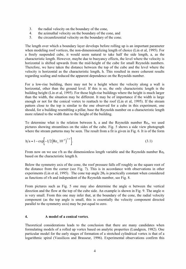
4

3. the radial velocity on the boundary of the cone,4. the azimuthal velocity on the boundary of the cone, and5. the circumferential velocity on the boundary of the cone.

The length over which a boundary layer develops before rolling up is an important parameterwhen modeling roof vortices, the non-dimensionalizing length of choice (Lin et al, 1995). Fora freely suspended cube, it would seem natural to take half the side length, a, as thecharacteristic length. However, maybe due to buoyancy effects, the level where the velocity ishorizontal is shifted upwards from the mid-height of the cube for small Reynolds numbers.Therefore, we have taken the distance between the top of the cube and the level where thevelocity is horizontal as the characteristic length, h. This resulted in more coherent resultsregarding scaling and reduced the apparent dependence on the Reynolds number.

For a low-rise building, there may not be a height where the velocity along a wall ishorizontal, other than the ground level. If this is so, the only characteristic length is thebuilding height (Lin et al, 1995). For those high-rise buildings where the height is much largerthan the width, the situation may be different. It may be of importance if the width is largeenough or not for the conical vortex to reattach to the roof (Lin et al, 1995). If the streampattern close to the top is similar to the one observed for a cube in this experiment, oneshould, for a building resembling a pillar, base the Reynolds number on a characteristic lengthmore related to the width than to the height of the building.

To determine what is the relation between h, a and the Reynolds number Rea, we usedpictures showing streamlines on the sides of the cube. Fig. 5 shows a side view photographwhere the stream patterns may be seen. The result from a fit is given in Fig. 6. It is of the form

h a =1� exp �1 2 Rea 10�5( )

3 / 4

[ ]. (3.1)

From now on we use r/h as the dimensionless length variable and the Reynolds number Reh

based on the characteristic length h.

Below the symmetry axis of the cone, the roof pressure falls off roughly as the square root ofthe distance from the corner (see Fig. 7). This is in accordance with observations in otherexperiments (Lin et al, 1995). The cone top angle 2�0 is practically constant when consideredas functions of r/h and independent of the Reynolds number, see Fig. 8.

From pictures such as Fig. 5 one may also determine the angle � between the verticaldirection and the flow at the top of the cube side. An example is shown in Fig. 9. The angle �is very small. From this one may infer that, at the boundary of the cone, the radial velocitycomponent (as the top angle is small, this is essentially the velocity component directedparallel to the symmetry axis) may be put equal to zero.

4. A model of a conical vortex.

Theoretical considerations leads to the conclusion that there are many candidates whenformulating models of a rolled up vortex based on analytic properties (Lundgren, 1982). Oneparticular model for the early stages of formation of a stretched cylindrical vortex is that of alogarithmic spiral (Vassilicos and Brasseur, 1996). Experimental observations confirm this

5

behavior (Petitjeans et al, 1996; Rossi et al, 2004). The kind of vortices considered in thispaper differs from these cylindrical vortices in one respect. For a conical vortex, there is astrong axial velocity component removing fluid that has been injected into the cone closer tothe tip.

The axial velocity component in a vortex induces an axial strain, favoring exchange of fluid inthe direction perpendicular to the axis of symmetry. This leads to an enhanced and more rapidmixing of the rolled boundary layers for a conical vortex compared to a cylindrical vortex. Itthen seems reasonable that, when modeling conical vortices, one may assume that the vortexpossesses a cylindrical symmetry, maybe with the exception of the outermost layer. This kindof models is common when modeling conical vortices (Banks et al, 2001). We have chosen tobase our model of a conical vortex on this assumption. However, some flattening of the vortexhas been experimentally observed (Banks and Meroney, 2001).

We seek a solution to the flow equations satisfying the boundary conditions that have beenderived in the previous sections. In the analysis, we will use spherical coordinates (r, �, �)with the origin at the building top corner. Thus, r will be the distance from this corner. Thevelocity in the r-direction is approximately parallel to the symmetry axis as the cone top angleis small. The azimuthal velocity (the �-direction) is perpendicular to the envelope of the coneand defines the flux of fluid into it. The circumferential velocity (the �-direction) defines therotation of the vortex. The velocity components relative the roof have been defined in Fig. 3.

The boundary conditions for the velocity components that we will consider have beendetermined as follows.

1. As noted above (Fig. 7), below the symmetry axis of the cone, the roof pressure fallsoff roughly as the square root of the distance from the corner. If the pressure isessentially determined by the square of the velocity u on the boundary, this velocitybehaves as

u r,� = �0( )� r h( )�1 4

. (4.1)

2. The radial velocity, ur , is almost zero on the boundary � = �0 (see Fig. 9).

The relevant flow equations are the Navier-Stokes equation and the equation of continuity foran incompressible fluid,

�tu + � � u +� u2 2 + p( ) �Re�1�u = 0, (4.2)

� � u = 0. (4.3)

In these equations, velocities are normalized by the free-stream velocity U, length coordinatesby h (see Section 3), time by h/U and pressure by �U2 2. Taking the rotation of eq. (4.2), oneof the non-linear terms (the gradient term) disappears. The other non-linear term, the onestemming from � � u , disappears if the velocity u and the vorticity � are parallel. However,this prescription needs to be cast in the form of an explicit equation to be useful. Such anequation is provided by the circumstance that the rotation of eq. (4.2) may be written in theform

6

�t� + u ��u � �(u) ��(�)( ) u � �( ) = Re�1�� . (4.4)

Here, the symbol �(u) indicates that the derivatives of the nabla operator are to be applied tothe components of u only. This equation and its equivalents are often referred to as thevorticity equation or the vorticity transport equation. As the non-linear terms on the left-handside disappear if the vorticity is parallel to the velocity, the remaining terms must satisfy thediffusion type equation

�t� = Re�1�� . (4.5)

This is possible if the velocity or the vorticity can be factorized with regard to spacecoordinates and time. For example, a vortex left to decay from time t=0 will have a factorexp �t Re( ) and a shear flow starting at time t=0 will create a growing vortex with a factor

1� exp �t Re( )[ ]. Denote the time dependent factor by f(t). A velocity field satisfying the

above requirements is given by

ur (r,�,t) = �Cl(l +1) r�1 j

l(r)R

l

0(�)f(t)

u� (r,�,t) = �C jl�1(r) � lr

�1 jl(r)[ ]R l

1 (�) f(t) (4.6)

u�(r,�,t) = C jl (r) R l

1 (�) f(t).

Here, C is a constant, jl

is a spherical Bessel function and Rl

m with m=0, 1 is an associateLegendre function. This velocity field satisfies the eq. (4.4). As a matter of fact, any linearcombination of velocity fields of the form of eq. (4.6) but displaced from the origin to anyother point or time will also satisfy eq. (4.6) (Lyberg and Tryggeson, 2007). Thiscircumstance allows a description of a dynamical vortex, such as the swaying of the mainaxis, or the influence on the vortex from gusts. Consider the simple example of a vortexdriven by a wind of constant direction but of varying speed U(t). In this case, the factor f(t)above would take the form

f(t) = exp �(t � �t ) Re[ ]U(t�)dt���

t

� . (4.7)

The relevant associated Legendre functions of eq. (4.6) may not have any zeros for arbitraryvalues of the parameter l. However, the second boundary condition stated above may be

satisfied by making the angular factors of u a linear combination of Legendre functions of thefirst and second kind

Rl

m (�) =Ql

0(�0)Plm (�) �P

l

0(�0)Ql

m (�), (4.8)

where m=0 or 1. From the velocity field given by eq. (4.6), one may now calculate thepressure from eq. (4.2)

p = �u2 2 + p� + Re�1

�u � d�

r

� r , (4.9)

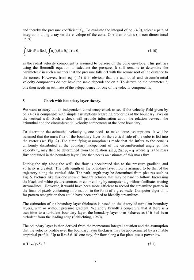
7

and thereby the pressure coefficient Cp. To evaluate the integral of eq. (4.9), select a path ofintegration along a ray on the envelope of the cone. One then obtains (in non-dimensionalunits)

�u � d�

r

� r = Re�t ur (r,� = �0) d�

r

� r = 0, (4.10)

as the radial velocity component is assumed to be zero on the cone envelope. This justifiesusing the Bernoulli equation to calculate the pressure. It still remains to determine theparameter l in such a manner that the pressure falls off with the square root of the distance to

the corner. However, from eq. (4.6) it is obvious that the azimuthal and circumferentialvelocity components do not have the same dependence on r. To determine the parameter l,

one then needs an estimate of the r-dependence for one of the velocity components.

5 Check with boundary layer theory.

We want to carry out an independent consistency check to see if the velocity field given byeq. (4.6) is compatible with simple assumptions regarding properties of the boundary layer onthe vertical wall. Such a check will provide information about the relation between theazimuthal and the circumferential velocity components at the cone boundary.

To determine the azimuthal velocity u� one needs to make some assumptions. It will beassumed that the mass flux of the boundary layer on the vertical side of the cube is fed intothe vortex (see Fig. 2). The simplifying assumption is made that the influx to the cone isuniformly distributed at the boundary independent of the circumferential angle �. Thevelocity u� may then be determined from the relation sin�0 2� r u� = q where q is the massflux contained in the boundary layer. One then needs an estimate of this mass flux.

During the trip along the wall, the flow is accelerated due to the pressure gradient, andvorticity is created. The path length of the boundary layer flow is assumed to be that of thetrajectory along the vertical side. The path length may be determined from pictures such asFig. 5. Pictures like this one show diffuse trajectories that may be hard to follow. Increasingthe black and white picture contrast or color coding by computer algorithms facilitates tracingstream-lines. However, it would have been more efficient to record the streamline pattern inthe form of pixels containing information in the form of a grey-scale. Computer algorithmsfor pattern recognition then could have been applied to identify streamlines.

The estimation of the boundary layer thickness is based on the theory of turbulent boundarylayers, with or without pressure gradient. We apply Prandtl’s conjecture that if there is atransition to a turbulent boundary layer, the boundary layer then behaves as if it had beenturbulent from the leading edge (Schlichting, 1960).

The boundary layer is then derived from the momentum integral equation and the assumptionthat the velocity profile over the boundary layer thickness may be approximated by a suitableempirical profile. Up to Re<3.6 106 one may, for flow along a flat plate, use a power law

u /U = (y /�)1/ n , (5.1)

8

where n is a constant depending on Re, U is the flow velocity outside the boundary layer and� is the boundary layer thickness. Taking n=7 should be valid for an interval in Re from 105 to3.2 106 and includes our experimental data interval. We will assume that this power lawprofile is valid.

In the presence of a pressure gradient, the boundary layer gets thinner than in the case of azero pressure gradient. However, in this approximate estimate, we will assume that theboundary layer may be treated as the one for a flat plate. We have chosen to identify theboundary layer thickness by the momentum thickness �2. It is defined as

�2 = u(y) /U (1� u(y) /U) dy0

�

� , (5.2)

where U is the flow velocity outside the boundary layer. A calculation using the eq. (5.1) and(5.2) yields the result that the boundary layer thickness after a path length s is

�(s) = 0.37 Reh�1/ 5(s /h)4 / 5h . (5.3)

The trajectory lengths have been determined from side view photographs. One finds that thelength s of trajectories such as those of Fig. 5 then depends on the distance r in the form of apower law,

s h =1.24 r h( )0.91

. (5.4)

This result is displayed in Fig. 10. Subsequently, we have therefore used the results of eq.(5.4) in all calculations.

Consider the volumetric flux, q, that is fed into the cone. The amount fed in must for a fixed rbe equal to the volume that the boundary layer contains at the edge of the wall for the same r,

q = u(y) dy0

�

� = U (y /�(s) )1/ n dy =U0

�

� �(s) n(n +1). (5.5)

The above assumptions that the flux of the boundary layer is fed into the vortex then leads to

sin�0 u� (r, � = �0) 2�r dr =U 0.37 Reh�1/ 5(s /h)4 / 5h n(n +1) dr . (5.6)

The velocity u�, may then be estimated assuming that the free stream velocity U isapproximately the same as the flow velocity outside the boundary layer along the wall. This isnot an exact relation as the fluid is accelerated when moving along the wall. The blockingeffect when inserting the bluff body into the wind-tunnel was 4%, which increases thevelocity outside the wall. The actual velocity enhancement rather was somewhat more than10%.

Inserting the result of eq. (5.4) into eq. (5.5) yields

sin�0 u� (r, � = �0) U� (r /h)�0.27, (5.7)

9

which is almost the same exponent as in eq. (4.6). A number of simplifying assumptions havebeen made in the calculation above, so this result should not be taken as a confirmation of thevalidity of eq. (4.6), but it gives an indication that the model is a sound one.

It remains to fix the value of the parameter l, which determines the r-dependence of the

velocity components. Guided by eq. (5.7), we put l=3/4, giving the azimuthal velocity the

dependence u� � r�1/ 4 . Fixing the value of this parameter, one may now calculate the two

angular functions Rl

m (�), m=0, 1 defined in eq. (4.8). The result is shown in Fig. 11.

6 Results and Discussion

In Section 4 the solution method was presented and from the calculations the velocity fieldwas determined. From that point of view the whole problem is solved, and to receive thewanted output, it is possible to determine the velocity field, the pressure field, and thevorticity. In the previous sections, a number of approximations and assumptions have beenmade regarding the character of the flow. A listing thereof includes the following items.

1. The vortex has been assumed to possess a rotational symmetry, neglecting any layeredstructure and flattening.

2. The characteristic length chosen is the distance between the roof and the height atwhich the wall boundary layer reaching the top commences its journey.

3. No effects of an atmospheric boundary layer are considered.4. In the model derived from a solution to the flow equations, there is no implicit

dependence on the Reynolds number, Re, except for the dependence on time.However, notice that we have still a Re-dependence from the boundary conditions.

5. The pressure is found to decrease as the inverse of the square root of the distance fromthe corner, r, motivating a dependence of the azimuthal velocity as u� � r

�1/ 4 .6. With the model chosen, the pressure on the boundary of the cone may be derived from

the Bernoulli equation.7. The external flow driving the vortex has been assumed to be quasi-stationary.

The static pressure coefficient, Cp, may be derived from equation (4.7).

Figure 12 shows the theoretically calculated values of -Cp and the experimentally measuredones for a value of Re=1.8 105 for a freely suspended cube. They agree remarkably well forvalues up to r/h=1, that is up to r=h in dimensional coordinates.

There are some remarks to be made. First, the boundary conditions are calculated from atheory of a simple boundary layer description involving the momentum thickness �2. Asecond remark is that our characteristic length, h, is dependent on Re, if the characteristiclength used in the definition of Re is related to the side length of the cube. It establishes theboundary conditions, and data has been taken from a freely suspended cube. But the generalmodel itself is not Re-dependent. The conclusion is that there is no simple scaling in Cp forRe, but it depends on details of the boundary layer rolling up to become a conical vortex.

10

References

Ahmad S., Kumar K., 2002. Wind pressures on low-rise hip roof buildings. Wind andStructures 5, 493-514.

Banks D., Meroney R.N., Sarkar P.P., Zhao Z., Wu F. 2000. Flow visualization of conicalvortices on flat roofs. J. Wind Eng. Ind. Aerodyn. 84, 65-85.

Banks D., Meroney R.N., 2001. A model of roof top surface pressures produced by conicalvortices. Wind and Structures 4, 227-246.

Bienkiewicz B., Ham H.J., 2003. Wind tunnel modelling of roof pressure and turbulenceeffects on the TTU test building. Wind and Structures 6, 91-106.

Cochran L.S. 1992. Wind tunnel modeling of low rise structures. Ph.D. Thesis, CivilEngineering, Colorado State University, CO.

Davenport, A.G., 1960. Wind Loads on Structures. NRCC 5576, Division of BuildingResearch, National Research Council of Canada, Ottawa, Canada.

Dogigalski, T.L., Smith, C.R., Walker, J.D.A., 1994. Vortex interactions with walls. Ann.Rev. Fluid Mech. 26, 573-616.

Franchini, S., Pindado, S., Meseguer, J., Sanz-Andres, A., 2005. A parametric, experimentalanalysis of conical vortices on curved roofs of low-rise buildings. J. Wind Eng. Ind. Aerodyn.93, 639-650.

Fu J.Y., Li Q.S., Xie Z.N., 2005, Wind effects on a large cantilevered flat roof. Wind andStructures 8, 357-372.

Hall, M. G., 1961. A theory for the core of a leading-edge vortex. J. Fluid Mech. 11, 209-228.

Kawai H., Nishimura G., 1996. Characteristics of fluctuating suction and conical vortices on aflat roof in oblique flow. J. Wind Eng. Ind. Aerodyn. 60, 211-225.

Kawai H., 1997. Structure of conical vortices related with suction fluctuation on a flat roof. J.Wind Eng. Ind. Aerodyn. 69-71, 579-588.

Kawai H., 2002. Local peak pressure and conical vortex on building. J. Wind Eng. Ind.Aerodyn. 90, 251-263.

Kind, R.J., 1986. Worst suctions near edges on flat rooftops on low-rise buildings, J. WindEng. Ind. Aerodyn. 25, 31-47.

Kramer C., Gerhardt, H.J., 1991. Wind pressures on roofs of very low and very largeindustrial buildings. J. Wind Eng. Ind. Aerod. 38, 285-295.

Lambourne, N.C., Bryer, D.W., 1959. Some measurements in the vortex flow generated by asharp leading edge having 65° sweep. Aero. Res. Coun., Document 477.

11

Lee, B.E., Evans, R.A., 1984. The measurements of wind flow patterns over building roofs.Building and Environment 4, 235-241

Letchford, C.W., Marwood, R., 1997. On the influence of v and w component turbulence onroof pressures beneath conical vortices. J. Wind Eng. Ind. Aerodyn. 69-71, 567-577.

Leufheusser, H.J., 1965. Pressure distributions on a cube at various degrees of boundary layerimmersion. Univ. of Toronto. U 1 Mec TP 6502.

Lin, J.X., Surry, D., Tieleman, H.W., 1995. The distribution of pressure near roof corners offlat roof low buildings, J. Wind Eng. Ind. Aerodyn. 56, 235-265.

Lundgren, T.S., 1982. Strained spiral vortex model for turbulent fine structure. Phys. Fluids25, 2193-2203.

Lyberg, M.D., Tryggeson, H., 2007. Analysis of 3-D vortex structures in fluids. Submitted toPhys. Rev. Lett.

Marwood R. 1996. An investigation of conical roof edge vortices. Ph.D. Thesis, LincolnCollege, Univ. of Oxford, Oxford, U.K.

Petitjeans P., Robres J.H., Wesfreid J.E., Kevlahan N., 1998. Experimental evidence for anew type of stretched vortex. Eur. J. Mech. B./Fluids 17, 549-560.

Rossi M., Bottausci F., Maurel A., Petitjeans P., 2004. A nonuniformly stretched vortex.Phys. Rev. Lett. 92, 4504-4507.

Schlichting, H., 1960. Boundary-layer theory. Mc-Graw-Hill.

Simui, E., Scanlan, R.H., 1978. Wind effects on structures: An introduction to windengineering. A Wiley-Interscience publication.

Tieleman, H.W., Surry, D., Metha, K.C., 1996. Full-model scale comparison of surfacepressures on the Texas Tech experimental building. J. Wind Eng. Ind. Aerodyn. 61, 1-23.

Vassilicos J.C., Brasseur J.G., 1996. Self-similar spiral flow structure in low Reynoldsnumber isotropic and decaying turbulence. Phys. Rev. E 54, 467-485.

Wirén, B., 1970. Wind-tunnel investigation of the pressure distribution on a flat roof forvarious roof edges (in Swedish). The National Swedish Institute for Building Research.Rapport R35.

Wirén, B.,1985. Effects of Surrounding Buildings on Wind Pressure Distributions andVentilation Losses for Single-Family Houses. Part I. The National Swedish Institute forbuilding research. Bulletin M85.

Wirén, B.,1990. Wind effects on structures, Lecture Notes on Building Aerodynamics (inSwedish). The National Swedish Institute for Building Research.

12

Wu F. Sarkar P.P., Mehta K.C., 2001. Full scale study of conical vortices and roof cornerpressures. Wind and Structures 4, 131-146.

Zhao Z., Sarkar P.P., Mehta K.C., Wu F., 2002. Wind flow characteristics and their loadingeffects on flat roofs of low-rise buildings. Wind and Structures 5, 25-48.

13

Fig. 1: The flow above the horizontal top of a cube at Re=105. The incoming flow isfrom the left. The two conical vortices are close to the edges.

Fig. 2: Sketch of conical vortices. The horizontal arrow indicates the wind direction.The other arrow indicates the leading edge.

14

Fig. 3: The pressure coefficient on a roof and definition of the x- and y- coordinateaxes. Half the top angle of the conical vortex usually takes a value between 11and 14 degrees in building aerodynamics. To the upper right, the velocitycomponents in spherical coordinates are indicated.

Fig. 4: Pressures measured below a vortex on top of a freely suspended cube. Thecurves have been obtained from a cubic spline fit. The pressure minimum isdetermined from the maximum of the curves. Data refer to the vortex close tothe y-axis (see Fig. 3).

15

Fig 5: Computer-modified picture of he flow along the wall at Re=105. Thecharacteristic length h is the distance between the top and the symmetry line ofthe cube. The symbol � indicates the angle between the boundary layer velocityand the normal to the top for the flow leaving the edge.

Fig. 6: A relation between the characteristic length and the half side of a cube, a, forvarious values of the Reynolds number Rea. The values of h have beendetermined from Schlieren photographs such as the one presented in Fig. 5.

16

Fig. 7: The value of �Cp r h as dependent on r/h for Reynolds numbers Reh in the

range 0.2<Reh 10-5<6.0. There is no systematic dependence on r/h found. The

scatter around the average value is about 7%.

Fig. 8: The dependence of half the vortex top angle on distance r/h. The average hereis 13 degrees.

17

Fig. 9: The direction of the flow leaving the wall. The angle � is the deviation from thevertical direction.

Fig. 10: A relation between the trajectory length as a function of r/h for variousReynolds numbers 0.2<Re 10-5<6.1. The values have been obtained fromSchlieren photographs.

18

Fig. 11: The radial functions Rl

m �( ) , m=0,1, for angles between 0 and �0=13°, or0.975<cos�<1. The solid line is m=0.

Fig. 12: A comparison between theoretical and experimental values of -Cp as a functionof r/h. The curve gives the pressure coefficient below the symmetry axis of theconical vortex at an angle of incidence equal 45°.

II

Analytical Solution of the Navier-Stokes Equation

for Internal Flows

Mats D. Lyberg and Henrik Tryggeson

Department of Physics, Vaxjo University, 35195 Vaxjo, Sweden.

E-mail: Mats.Lyberg@msi.vxu.se, htr@msi.vxu.se

Abstract. This paper derives a solution to the Navier-Stokes equation by consideringvorticity generated at system boundaries. The result is an explicit expression for thevelocity. The Navier-Stokes equation is reformulated as a divergence and integrated,giving a tensor equation that splits into a symmetric and a skew-symmetric part.One equation gives an algebraic system of quadratic equations involving velocitycomponents. A system of non-linear partial differential equations is reduced to algebra.The velocity is then explicitly calculated and shown to depend on boundary conditionsonly. This removes the need to solve the Navier-Stokes equation by a 3-D numericalcomputation, replacing it by computation of 2-D surface integrals over the boundary.

PACS numbers: 47.10.-g, 47.10.A-, 47.10.ab, 47.10.ad

Analytical Solution of the Navier-Stokes Equation for Internal Flows 2

A major obstacle for detailed calculations of fluid flows is the time consuming

3-D calculations characteristic of solving differential equations numerically, or using

integral methods involving the calculation of entire 3-D domain integrals. For the

latter approach, various methods have been presented that attempt to reduce the

computational task. In the boundary element method one applies potential theory

to lower the dimension of the problem by one order. However, this property is lost

if vorticity is considered. An extended version of the method [1], transforms local

boundary conditions into global conditions integrated over the boundary. The velocity

is divided into a potential and a rotational part. This leads to a system of coupled

boundary integral equations to be solved iteratively. The property of the reduced

dimension is preserved. Other methods, commonly applied to vibration analysis, also

transforming domain integrals into boundary integrals include the dual reciprocity

method [2], and the particular integrals technique [3]. The application of these latter

methods is limited to small values of the Reynolds number [4, 5].

Laboratory experiments indicate the significant role played by the no-slip boundary

condition in the formation of vortex filaments affecting the flow evolution. Recently, [6],

detailed studies of vortex filaments in 2-D turbulent flows reveal that their influence

may have dramatic effects on the flow, not only in the vicinity of the wall but extending

over the full flow domain

It is a common assumption that to describe quantitatively turbulent flows in the

presence of solid boundaries, it is necessary to have a quantitative model of the vorticity

creation rate [7]. Based on this assumption, the boundary vorticity dynamics model has

developed [8], describing the vorticity creation from solid boundaries and the reaction of

the created vorticity to the boundaries. In this model, the velocity field is decomposed

into two parts. One part, derived from a scalar potential, describes the longitudinal

compression. The other part, derived from a vector potential, describes the transverse

shearing process.

None of the methods or models listed in the previous paragraphs yields a closed

expression for the velocity in the flow in terms of conditions at the system boundary.

Such an expression is presented in this work. We do not a priori assume any explicit

model of vorticity formation, or that the velocity field may be split into a potential and

a rotational part.

From a strictly mathematical point of view, it may not be straightforward how to

solve a set of non-linear partial differential equations and include boundary conditions.

From a physical point of view, the situation is simpler. The Navier-Stokes equation

describes the acceleration of a fluid subjected to interior forces. If the validity of the

equation is extended to include also the boundary, the external pressure and viscous

forces at the boundary have to be included in the equation. It then describes the

acceleration in a system exposed to interior and external forces. A common procedure

then is to integrate the equation. We have done just that.

The Navier-Stokes is recast in the form of a divergence that is zero, permitting

immediate integration. By invoking symmetry properties, the resulting expression may

Analytical Solution of the Navier-Stokes Equation for Internal Flows 3

be partitioned into two equations that may be solved separately. One equation gives a

linear partial differential equation for the velocity potential, permitting the calculation

of a rotational part of the velocity field. The other equation reduces to a quadratic

algebraic equation for components of a velocity field. These two solutions may be added,

giving in closed form an expression only depending on externally applied pressure and

the value of the velocity and the derivatives of the velocity at the boundary.

The flow of an incompressible fluid of velocity u(r, t) is governed by the Navier-

Stokes equation (1) and by the equation of continuity (2). These equations are most

often formulated as

ρ∂tu + ρ (u · ∇) u ≡ ρ∂tu + ρω × u +1

2∇ρu2 = −∇p − μ∇× ω , (1)

ρ∇ · u = Q(r′, t′)δ(r − r′)δ(t − t′) . (2)

Here, ω = ∇ × u is the vorticity, p the pressure, ρ the density, μ the viscosity,

and Q(r′, t′) the amount of fluid injected into sources or removed by sinks from the

system at a specified point and time. If the vorticity is considered as a skew-symmetric

tensor, ωji = ∂jui − ∂iuj, a conjugate variable is the rate of strain, σ, defined from

σji = ∂jui+∂iuj. The Navier-Stokes equation is the law of force where the left hand side

contains the acceleration and the right hand side the forces acting in the system. The

density and the viscosity will be treated as constants. It follows from Eq. (2) that the

Helmholtz decomposition applies, the velocity u is uniquely defined from an rotational

part urot determined by a vector potential A, and a potential part upot determined by

a scalar potential φ as

u = urot + upot = ∇× A + ∇φ . (3)

Here, φ has to satisfy the Laplace equation Δφ = 0 if there are no sources and sinks.

The vorticity is determined from the vector potential as ω = ∇(∇ · A) − ΔA. It is

possible to choose A such that ∇ · A = 0 (see [9], for a discussion on the uniqueness of

the Helmholtz decomposition).

The Eq. (1) describes the flow in a free space, but contains no information about

how to take into account boundary conditions. We will integrate Eq. (1) and therefore

include on its right hand side the forces acting on the fluid at the boundary. These

forces include pressure applied at inlets and outlets and viscous forces at boundaries.

We rewrite Eq. (2) to describe fluid entering or leaving the system at points rQ on

the boundary

ρ∇ · u(r, t) = 2Δ(r)

∫∫dSQ · u(rQ, t′)ρG(r − rQ)δ(t − t′) . (4)

The integration is over all surfaces Q of inlets and outlets where the entrance, or exit,

flow velocity is u(rQ). Here, G is the kernel, or Green’s function, G(r) = (4πr)−1. As

we are considering an incompressible fluid, the system responds instantaneously to any

dynamical change of external pressure or the flow from sources. This justifies the use of

a stationary Greens function in Eq. (4) satisfying the Laplace equation ΔG(r) = −δ(r).

Analytical Solution of the Navier-Stokes Equation for Internal Flows 4

This would give a minus sign to the right hand side of Eq. (4). However, another minus

sign enters because the surface element vector dSQ points away from the system. The

factor of 2 enters because when positioning point sources from Eq. (2) on a boundary

surface, only half the flux will enter the system, the other half ”on the other side of the

wall” will contribute to the environment. We rewrite Eq. (4) as

ρ∂juj(r, t) − ∂j∂

j2

∫∫dSQ · u(rQ, t′)ρG(r − rQ)δ(t − t′) = 0 . (5)

Here, we have applied a convention, a summation is to be carried out over identical

upper and lower indices. Next, we multiply this equation by the i-component of the

velocity. Using simple derivation rules and applying the fact that the second term of

Eq. (5) is zero except at inlets and outlets, one arrives at

ρuj∂jui = ρ∂j(u

jju

i) − ∂j∂j2

∫∫dSQ · u(rQ, t′)ui(rQ, t′)ρG(r − rQ)δ(t − t′) . (6)

The left hand side of Eq. (6) is identical to the second non-linear term of Eq. (1).

If one performs one of the derivations of the integral of Eq. (6) and then performs a

partial integration, the resulting expression will contain partial derivatives of the velocity

components.

We continue by adding to the right hand side of Eq. (1) the forces acting on the

system at the boundary in the form of an externally applied pressure at inlets and

outlets, and viscous stress acting at the boundary. Suppose we maintain at a point rQ,

belonging to an inlet or outlet, a pressure p(rQ, t′) applied in the direction −nQ if nQ

is directed from the fluid. One should then complement Eq. (1) on the right hand side

with a term −nQp(rQ, t′)δ(r − rQ)δ(t − t′).The force from viscous stress at surface element dSB at a point rB on the boundary

is given by the term μdSB×[∇×u(r, t)δ(r−rB)] = μ∇[u(r, t)δ(r−rB)·dSB]−μ[dSB ·∇]u(r, t)δ(r − rB) = μdSB · ∇u(r, t)δ(r − rB), an expression defining the dynamic

viscosity μ. The last equality is obtained if the boundary conditions are satisfied.

Writing these two contributions to the right hand side of Eq. (1) with the help of

Green’s functions, one arrives at the contribution

∂j∂j2

∫∫G(r − rQ)p(rQ, t)dSQ − μ∂j∂

j2

∫∫G(r − rB)dSB · ∇u(r = rB, t) , (7)

where the surface integrals are to be performed over the interior of the system boundary.

One may now collect terms from Eq. (6) and (7) by defining the tensors P , S and Ω

P ji = −2∂j

∫∫p(rp, t)G(r − rp)dSi

p , (8)

Rji = ∂j

∫∫G(r − rB)dSB · (μ∇− ρu)ui(rB, t) , (9)

Ωji = Rji − Rij = εijkΩk and Sji = Rji + Rij . (10)

Analytical Solution of the Navier-Stokes Equation for Internal Flows 5

The tensor Ω is skew-symmetric and is related to the amount of vorticity transferred

to the system, or generated, at boundaries. The first relation of Eq. (10) defines the

vector Ω. The tensor S is symmetric and related to to the amount of rate of strain

transferred to the system, or generated, at boundaries. The tensor P may be shown

to be approximately diagonal if the pressure force as well as the bulk flow is normal to

the surface, and neglects transverse pressure gradients across an inlet or outlet. In the

definition of these tensors, the area of inlets and outlets has been assumed situated at

the system boundary. The trace, the sum of the diagonal elements, of the tensors S and

Ω, tr(S) and tr(Ω), are zero.

Collecting all terms from the Eq. (3), (6) and (7), Eq. (1) may be rewritten for

the i-component as

∂j

[ρ∂tφδij + ρ∂tε

ijkAk + ρuiuj + pδij + μεijkωk +(Sji + P ji + Ωji

)δ(t − t′)

]= 0 , (11)

where εijk is the completely skew-symmetric Levi-Civita tensor. The Eq. (11) has the

form of a divergence being zero. Now, as stated after Eq. (2), the disappearing of the

divergence leads to the existence of potentials. Applying this result to Eq. (11) leads

to an equation for a second rank tensor. The expression inside the brackets of Eq. (12)

must be equal to a second rank tensor T satisfying ∂jTij = ∂iT

ij = 0. That equation

may be split into its symmetric and skew-symmetric parts yielding the two equations

ρ∂tφδij +[ρuiuj + pδji + P ij + Sij

]δ(t − t′) = T ij , (12)

εijkρ∂tAk − μεijkΔAk + Ωjiδ(t − t′) = εijkBk , (13)

where T is an arbitrary symmetric tensor and B an arbitrary irrotational vector.

Lowering one index and contracting Eq. (12) gives the relation

∂tρφD + ρu2 + pD + tr(P ) = tr(T ) , (14)

where D is the space dimension of the system. This equation is employed to calculate

the pressure in the flow. It remains to treat the case of the non-diagonal elements of

Eq. (12), that is the case i �= j, and the Eq. (13).

The off-diagonal part of Eq. (12) now reads

ρuiuj + P ij + Sij = T ij , (15)

which yields a non-linear, but purely algebraic, equation for the velocity components.

This equation has the solution U with components

U i(r, t) = ±√

ΣijΣik

Σjk, (16)

where Σnm = (−P nm−Snm+T nm)ρ

with i �= j �= k. This velocity is, in general, not

irrotational.

Analytical Solution of the Navier-Stokes Equation for Internal Flows 6

Eq. (13) is a linear differential equation for the vector potential A. To solve this

equation, employ the integral kernel of the diffusion equation, K(r, t), given in the form

(μΔ − ρ∂t)K(r, t) = −δ(r)δ(μt) ⇒ K(r, t) =exp

(− r2

4νt

)(4πνt)

D2

, (17)

where D is the space dimension and ν = μρ

is the kinematic viscosity. Multiplied by a

unit vector, K defines a solenoidal vector potential. Vortex models derived from this

kind of potential have been shown to account for the decay of vortex singlets generated

in a tank [10]. Models of vortex doublets derived from this kind of vector potential

reproduce the energy spectrum of 2-D turbulent flows generated in the laboratory [11].

The solution of Eq. (13) then reads

A(r, t) =

∫ t

0

νdt′∫∫∫

d3x′K(r − r′, t − t′) [Ω(r′, t′) − B(r′, t′)] =

∇×∫ t

0

νdt′∫∫

Γ (r − rB, t − t′) dSB · ∇u(r = rB, t′)

−∫ t

0

νdt′∫∫∫

d3x′K (r − r′, t − t′) B(r′, t′) . (18)

The second equality is obtained after integration over all space and using the fact that

the velocity is zero on the boundary. Thus, the vector potential describes vorticity

generated at solid boundaries as well as that contained in fluid entering or leaving the

system.

The function Γ is a solution to Δ(r)Γ(r − rB, t) = −K(r − rB, t), and is given by

Γ(r, t) = G(r)erf(

r√4νt

), where erf is the error function.

The rotational contribution to the internal velocity field from vorticity created at

the boundary, V , may now be determined by taking the rotation of the vector potential

of Eq. (18)

V (r, t) =

∫ t

0

νdt′[ ∫∫

K(r − rB, t − t′)dSB · ∇(rB)u(rB, t′)

−∇×∫∫∫

d3x′K (r − r′, t − t′) B(r′, t′)]

. (19)

This velocity field defines a rotational part of the velocity in terms of the externally

applied pressure and the value of the velocity and derivatives of the velocity at boundary

points.

To compute the velocity field from Eq. (16) and (19), one needs information about

the velocity and velocity gradients at the boundary. One way to obtain this information

is to find a solution to the equation of continuity, Eq. (2) satisfying the no-slip boundary

conditions, the velocity at the boundary must be zero. One may proceed as follows. The

bulk flow between inlets and outlets in an infinite space is given by the velocity field

vQ(r, t) = 2

∫∫dSQ · ∇(r)G(r − rQ)v(rQ, t) . (20)

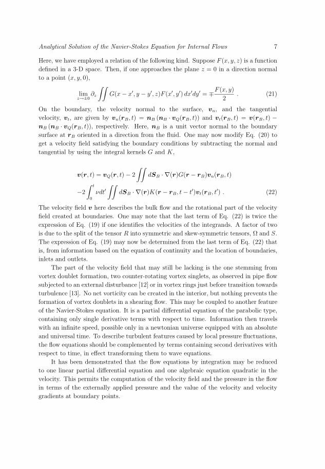
Analytical Solution of the Navier-Stokes Equation for Internal Flows 7

Here, we have employed a relation of the following kind. Suppose F (x, y, z) is a function

defined in a 3-D space. Then, if one approaches the plane z = 0 in a direction normal

to a point (x, y, 0),

limz→±0

∂z

∫∫G(x − x′, y − y′, z)F (x′, y′) dx′dy′ = ∓F (x, y)

2. (21)

On the boundary, the velocity normal to the surface, vn, and the tangential

velocity, vt, are given by vn(rB, t) = nB (nB · vQ(rB, t)) and vt(rB, t) = v(rB, t) −nB (nB · vQ(rB, t)), respectively. Here, nB is a unit vector normal to the boundary

surface at rB oriented in a direction from the fluid. One may now modify Eq. (20) to

get a velocity field satisfying the boundary conditions by subtracting the normal and

tangential by using the integral kernels G and K,

v(r, t) = vQ(r, t) − 2

∫∫dSB · ∇(r)G(r − rB)vn(rB, t)

−2

∫ t

0

νdt′∫∫

dSB · ∇(r)K(r − rB, t − t′)vt(rB, t′) . (22)

The velocity field v here describes the bulk flow and the rotational part of the velocity

field created at boundaries. One may note that the last term of Eq. (22) is twice the

expression of Eq. (19) if one identifies the velocities of the integrands. A factor of two

is due to the split of the tensor R into symmetric and skew-symmetric tensors, Ω and S.

The expression of Eq. (19) may now be determined from the last term of Eq. (22) that

is, from information based on the equation of continuity and the location of boundaries,

inlets and outlets.

The part of the velocity field that may still be lacking is the one stemming from

vortex doublet formation, two counter-rotating vortex singlets, as observed in pipe flow

subjected to an external disturbance [12] or in vortex rings just before transition towards

turbulence [13]. No net vorticity can be created in the interior, but nothing prevents the

formation of vortex doublets in a shearing flow. This may be coupled to another feature

of the Navier-Stokes equation. It is a partial differential equation of the parabolic type,

containing only single derivative terms with respect to time. Information then travels

with an infinite speed, possible only in a newtonian universe equipped with an absolute

and universal time. To describe turbulent features caused by local pressure fluctuations,

the flow equations should be complemented by terms containing second derivatives with

respect to time, in effect transforming them to wave equations.

It has been demonstrated that the flow equations by integration may be reduced

to one linear partial differential equation and one algebraic equation quadratic in the

velocity. This permits the computation of the velocity field and the pressure in the flow

in terms of the externally applied pressure and the value of the velocity and velocity

gradients at boundary points.

Analytical Solution of the Navier-Stokes Equation for Internal Flows 8

References

[1] Machane R, Achard J and Canot E 2000 Int. J. Num. Meth. in Fluids 34 47[2] Nardini D and Brebbia C A 1982 Boundary Element Methods in Engineering (Southampton, C.A.

Brebbia, Computational Mechanics Publ.) 157–171[3] Ahmad S and Banerjee P K 1986 J. of the Eng. and Mech. Div. ASCE 112 682[4] Zheng R, Phan-Thien N and Coleman J 1991 Comp. Mech. 8 71[5] Power H and Patridge P W 1994 Int. J. Num. Meth. Eng. 37 1825[6] van Heijst G J F, Clercx H J H and Molenar D 2006 J. Fluid. Mech. 554 411[7] Lighthill M J 1963 Boundary Layer Theory (Oxford, Oxford Univ. Press) 46–113[8] Wu J Z and Wu J M 1998 Theor. Comp. Fluid Dyn. 10 459[9] Dassios G and Lindell I V 2002 J. Phys. A 35 5139

[10] Trieling R R and van Heijst G J F 1998 Fluid Dynamics Res. 23 27[11] Tryggeson H and Lyberg M D 2007 submitted to Phys. Rev. Lett.[12] Hof B, van Doorne C W H, Westerweel J and Nieuwstadt F T M 2005 Phys. Rev. Lett. 95 214502[13] Dazin A, Dupont P and Stanislas M 2006 Exp. in Fluids 41 401

III

Vortex Evolution in 2-D Fluid Flows

Henrik Tryggeson and Mats D. Lyberg

Department of Physics, Vaxjo University, 35195 Vaxjo, Sweden

(Dated: February 22, 2007)

Abstract

Evolving 2-D turbulence is dominated by vortex structures. Experimental study of this phe-

nomenon is difficult, but some methods yield information on the dynamics of 2-D vortices. Avail-

able data include information on the structure of the velocity field, the growth rate and decay

rate of vortex structures, and energy spectra. It is proposed that all these features from different

experimental environments may be described by singlet or doublet vortex structures derived from

one unique vector potential. Predicted properties are confronted with experimental observations

on forced and decaying 2-D vortex systems.

PACS numbers: 47.32.C-, 47.27.-i

1

How turbulence arises and what role the creation and diffusion of vorticity plays in

this process is not well understood, neither in outline nor in detail. Any progress towards

an understanding of the fundamentals involved could be of great practical interest, for

example, for applications in astrophysics and geophysics. 2-D vortices have been observed

in nature, such as high and low pressure cells in the atmosphere, and oceanic eddies. The

formation of vortices is experimentally established as a distinct property of 2-D turbulent

flows. The mutual advection of well-separated vortices and the merger of like-sign vortices

are characteristic features.

Two common ways of experimentally generating quasi-2D turbulence are generation in a

thin layer of fluid and generation in a rapidly flowing soap film. In the first case a rotational

motion is induced by inserting a rotating solid object, or by introducing fluid jets. In the

other flow one may introduce comb-like structures into the fluid and vorticity is generated

at the boundary. For a review of experimental methods and results, see Ref. [1, 2].

Generation of vortex singlets in a tank within a layer of a stratified fluid yields vortex

structures that are not exact 2-D objects, but rather flat, pancake-like structures [3]. The

presence of solid boundaries act as sources of vortex filaments that by entering the flow may

significantly affect the flow evolution [4].

Another way of creating rotational flow is by electromagnetically driving flows in thin,

stable stratified layers [5, 6]. The flow is generated in a square cell by placing permanent

magnets at the bottom below an electrically conducting fluid and applying a voltage across

the fluid. In order to ensure two dimensionality, the cell is filled with layers of NaCl solutions

with different densities. The interaction of an electric current driven across the cell with the

magnetic field produces local stirring forces. It is possible to obtain data on the decay of

2-D vortices [5], the size and growth of and distance between vortex structures [7], as well

as energy spectra [8]. With this experimental set-up, friction with the bottom may affect

observations [6].

An alternative experimental approach is the use of flowing soap films [9]. Combs are

positioned in the flow, or at the boundaries of the flow, of a soap film falling vertically

between two wires under the influence of gravity. The teeth of the comb perpetually generate

small vortices, which are then quickly swept into the center of the channel by larger vortices.

The velocity fluctuations appear in the plane of the film, which has a thickness of μm,

whereas the radius r of eddies produced by the combs range from sub-mm to mm. A forced,

2

steady turbulent state ensues. Downstream from the forcing section of the channel, the

turbulence decays freely. Data on scaling effects [10] and energy spectra [11] have been

obtained.

The two equations governing the flow u (r, t) of an incompressible fluid are the Navier-

Stokes equation and the equation of continuity

∂tu + (u · ∇) u = −ρ−1∇p + ν∇2u , (1)

∇ · u = 0 . (2)

Here, ω = ∇ × u is the vorticity, p the pressure, ρ the density, ν the kinematic viscosity.

To eliminate the pressure, take the rotation of Eq. (1). One then arrives at the vorticity

transport equation that may be cast in the form

∂tω + u × Δu − (∇u −∇ω) (u · ω) = ν∇2ω , (3)

where the symbol ∇u indicates that the derivatives of the nabla operator are to be applied to

the components of u (r, t) only. In 2-D flows, the velocity is perpendicular to the vorticity,

so u ·ω = 0. We will restrict treatment to cases such that the remaining non-linear term of

Eq. (3) is either exactly zero, or can be shown to be so small that it may be neglected. The

equation then takes the form of the diffusion equation. The solutions may be derived from

a solenoidal vector potential A (r, t). We have applied the vector potential

A(r, t) = A(r, θ, t)e =rn cos nθ

(νt)βF (ξ)e , (4)

where ξ = r√νt

and n is an integer giving the order of the vortex multiplet, e is a unit vector,

β is a parameter characterizing the dynamic behaviour, F is a function of the diffusive

variable ξ. It remains to determine the function F . The velocity is given by the rotation

of this vector potential, and the vorticity is obtained by applying the Laplace operator to

the vector potential, ω = −ΔA. Similar vortex models have been shown to account for the

decay of vortex singlets generated in a tank [3].

Inserting the vorticity as described above, into Eq. (3) gives one solution

F (ξ) =∑

j

(ξ2

)j Γ(

n2

+ j − β)

(n + j)!j!, (5)

3

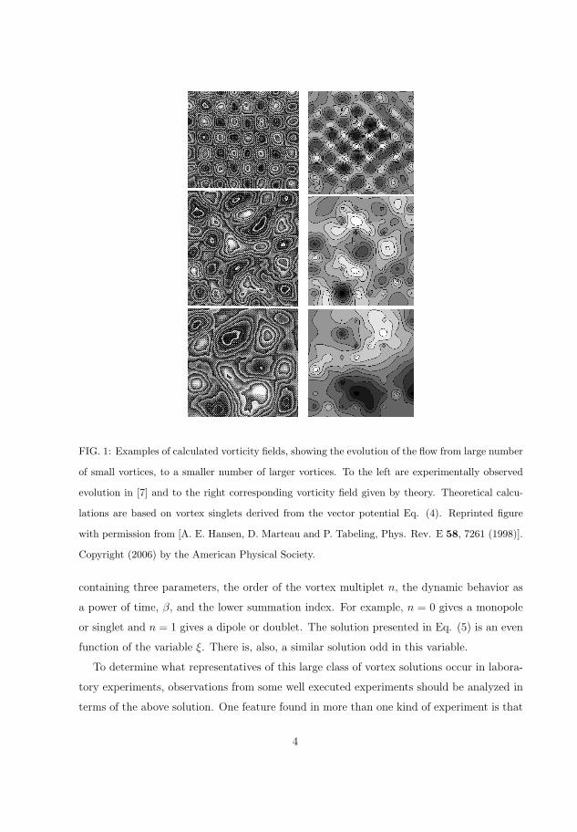
FIG. 1: Examples of calculated vorticity fields, showing the evolution of the flow from large number

of small vortices, to a smaller number of larger vortices. To the left are experimentally observed

evolution in [7] and to the right corresponding vorticity field given by theory. Theoretical calcu-

lations are based on vortex singlets derived from the vector potential Eq. (4). Reprinted figure

with permission from [A. E. Hansen, D. Marteau and P. Tabeling, Phys. Rev. E 58, 7261 (1998)].

Copyright (2006) by the American Physical Society.

containing three parameters, the order of the vortex multiplet n, the dynamic behavior as

a power of time, β, and the lower summation index. For example, n = 0 gives a monopole

or singlet and n = 1 gives a dipole or doublet. The solution presented in Eq. (5) is an even

function of the variable ξ. There is, also, a similar solution odd in this variable.

To determine what representatives of this large class of vortex solutions occur in labora-

tory experiments, observations from some well executed experiments should be analyzed in

terms of the above solution. One feature found in more than one kind of experiment is that

4

the energy spectral function E(k), where k is the wave number, shows a E(k) ∼ k−3 behav-

ior at least in the wave number range between 1 and 30 cm−1 [8, 11]. We investigate what

are the conditions for velocity fields derived from the vector potential Eq. (4) to reproduce

such a behavior.

The energy spectral function E(k) is defined from the relation

2πkE(k) =

∫ ∞

0

r dr

∫ 2π

0

u2 (r, t) eikr cos θ dθ . (6)

The velocity squared derived from Eq. (4) produces terms with the angular dependence

sin2 nθ and cos2 nθ. Carrying out the angle integration of Eq. (6) yields terms with Bessel

functions J2n(kr) and J0(kr). It remains to carry out the integration over r. Obviously, the

velocity squared can only produce even powers of r, for example a power of 2M . Introducing

some coefficients C(n, β, M), which may be calculated from Eq. (4), Eq. (6) may now be

written

E(k) =

∫ ∞

0

rdr∑M

C(n, β, M)r2n−2+2M t−M [c1J2n(kr) + c2J0(kr)]

=∑M

C(n, β, M)k−3−2M t−M

[c1

22n(n + M)!

Γ(n − M)+ c2

M !

Γ(−M)

]. (7)

The singularity of the Γ-function at zero and negative integers means that the contribution

from vortex singlets is zero. Vortex multipoles, n > 0, produce the desired behavior but

only for M = 0. Contributions from terms with powers of r greater than 0 fall off as powers

of k larger than 3. Also, such terms disappear more quickly with time. Information on the

rate of fall-off with time is required to determine the value of the parameter β.

We start comparison to experimental data by considering vorticity generated in layered

media. In one experiment [7] vortices have been generated an 8× 8 array of a bounded 2-D

space, with nearest neighbors counter-rotating. It is then possible to follow the diffusion of

vorticity at different times and the qualitative evolution of the flow from a large number

of small vortices to a small number of large vortices. To reproduce the patterns of this

evolving flow field, we carried out a simulation by placing a number of vortex singlets in

the same manner as used in the experiment. We used vortex singlets derived from the

vector potential Eq. (4) with a simple vortex singlet, putting n = 0 and β = −12. Two

counter-rotating vortex singlets of this kind produce the vortex dipole n = 1 and β = 0.

5

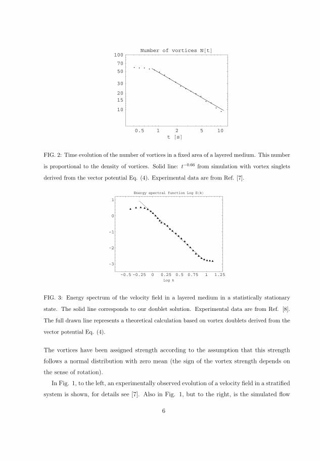
0.5 1 2 5 10t �s�

10

1520

30

50

70

100Number of vortices N�t�

FIG. 2: Time evolution of the number of vortices in a fixed area of a layered medium. This number

is proportional to the density of vortices. Solid line: t−0.66 from simulation with vortex singlets

derived from the vector potential Eq. (4). Experimental data are from Ref. [7].

-0.5 -0.25 0 0.25 0.5 0.75 1 1.25Log k

-3

-2

-1

0

1

Energy spectral function Log E�k�

FIG. 3: Energy spectrum of the velocity field in a layered medium in a statistically stationary

state. The solid line corresponds to our doublet solution. Experimental data are from Ref. [8].

The full drawn line represents a theoretical calculation based on vortex doublets derived from the

vector potential Eq. (4).

The vortices have been assigned strength according to the assumption that this strength

follows a normal distribution with zero mean (the sign of the vortex strength depends on

the sense of rotation).

In Fig. 1, to the left, an experimentally observed evolution of a velocity field in a stratified

system is shown, for details see [7]. Also in Fig. 1, but to the right, is the simulated flow

6

field described above. Visually, the patterns are similar. Turning to a more quantitative

comparison, the number of vortices is reduced with time while their average size grows. A

best fit to the vortex density ρ(t) and the average vortex radius a(t) obtained from the

simulation gives

ρ(t) ∼ t−0.66±0.10, a(t) ∼ t0.30±0.10 . (8)

The exponents determined here, −0.66± 0.10 for the density of vortices and 0.30± 0.10 for

the vortex radius should be compared to those obtained experimentally in a stratified flow

field [7], −0.70±0.10 and 0.21±0.06, respectively. Thus, there is a good agreement between

experiment and theory when it regards describing the pattern of the most prominent vortex

singlets. The result of this simulation is presented in Fig. 2.

Vortex singlets do not give any contribution to the energy spectrum, as noted above.

This argument was based on the assumption that the vortex singlet was situated in an

infinite space. As seen in Fig. 1, the vortex singlets there are rather local, and should not

be expected to be of any strength outside a limited region. Therefore, there contribution to

the energy spectrum may probably be neglected. In Fig 3, the experimental values of the

energy spectra of a stratified system [8] are presented together with the contribution from

a vortex doublet n = 1, β = 0, the vortex doublet derived from vortex singlets discussed

in the previous two paragraphs. The vortex solution predicts quite well the slope of the

experimentally statistically stationary turbulent state. For wave numbers smaller than 1

cm−1, the energy spectral density is experimentally found to be flat, maybe reflecting a

limitation in resolving experimentally low velocity levels at small scales [8].

One may conclude that interference between strong counter-rotating vortex singlets leads

to an energy spectral function dominated by contributions from vortex dipoles.

We now turn to a discussion of results using the experimental technique a flowing soap

film between partially cambered walls [11]. Regard the velocity profile as being produced by

vortices. We assume that the vorticity generated at the edges of the channel decays while

being carried downstream, but this is compensated for by new vorticity generated along the

boundaries. With this view, the vorticity at a station should consist of vortices generated

since the onset of the flow. A schematic picture presenting the above argument is given

in Fig. 4. One would expect that in the absence of combs, the velocity profile would be

parabolic, as for plane Poiseuille flow, generated by vortex doublets of the same kind as when

7

+ =

FIG. 4: Schematic picture of the assumed constituents of the flow field in a channel with combed

walls. The stationary part of the flow is assumed to consist of a uniform flow represented by the

arrows to the left. Vorticity is created by the combs at the boundary of system of the falling soap

film. Vortex structures created at the boundary and leaving the boundary, entering the bulk flow,

are assumed to be described by vortex doublets. Vortices of this structure build up a parabolic

velocity profile if constantly created in the absence of combs, and the combined flow satisfies the

no-slip boundary condition.

combs are present, but much weaker. The vorticity must be described as vortex doublets in

order that no-slip boundary conditions are satisfied. To arrive at a parabolic profile, built up

by vortex contributions from different times and the stationary uniform velocity component,

one should have for the flow in the x-direction

ux =

∫uθ

(θ =

π

2, t

)dt = 1 − y2 . (9)

We apply the same vortex doublet that was used in the analysis of the layered media.

Analysis of the solution gives us some predictions for the energy spectral function E(k)

obtained at different times t:

1. the energy spectral function E(k), as a function of k, scales with k√

νt,

2. it has an amplitude that is proportional to νt, and

3. it decays with wave number k as E(k) ∼ k−3.

In Fig. 5, the experimental energy spectra for different positions downstream from the

combs are presented. This can be compered with the scaled values given in Fig. 6. For

the dominant term we find the slope E(k) ∼ k−3 which is also dispayed in Fig. 5. This

8

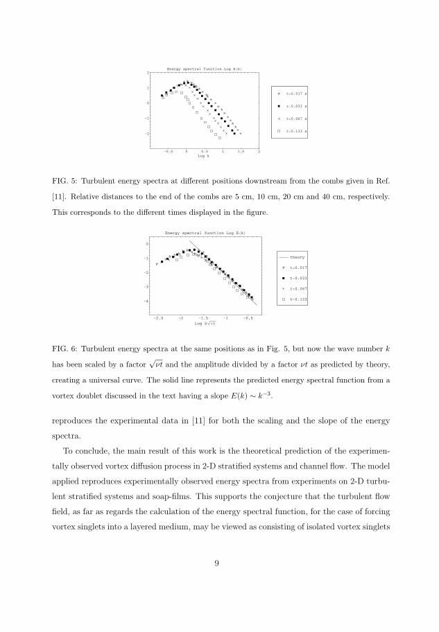
-0.5 0 0.5 1 1.5 2Log k

-2

-1

0

1

2Energy spectral function Log E�k�

t�0.133 s

t�0.067 s

t�0.033 s

t�0.017 s

FIG. 5: Turbulent energy spectra at different positions downstream from the combs given in Ref.

[11]. Relative distances to the end of the combs are 5 cm, 10 cm, 20 cm and 40 cm, respectively.

This corresponds to the different times displayed in the figure.

-2.5 -2 -1.5 -1 -0.5

Log k�Νt

-4

-3

-2

-1

0

Energy spectral function Log E�k�

t�0.133

t�0.067

t�0.033

t�0.017

theory

FIG. 6: Turbulent energy spectra at the same positions as in Fig. 5, but now the wave number k

has been scaled by a factor√

νt and the amplitude divided by a factor νt as predicted by theory,

creating a universal curve. The solid line represents the predicted energy spectral function from a

vortex doublet discussed in the text having a slope E(k) ∼ k−3.

reproduces the experimental data in [11] for both the scaling and the slope of the energy

spectra.

To conclude, the main result of this work is the theoretical prediction of the experimen-

tally observed vortex diffusion process in 2-D stratified systems and channel flow. The model

applied reproduces experimentally observed energy spectra from experiments on 2-D turbu-

lent stratified systems and soap-films. This supports the conjecture that the turbulent flow

field, as far as regards the calculation of the energy spectral function, for the case of forcing

vortex singlets into a layered medium, may be viewed as consisting of isolated vortex singlets

9

creating vortex doublets when interfering. For the case of channel flow vortex doublets are

created at the system boundary and quickly swept into the main stream by larger vortices.

[1] P. Tabeling, Phys. Rep. 362, 1 (2002).

[2] H. Kellay and W. I. Goldburg, Rep. on Progr. in Phys. 65, 845 (2002).

[3] R. R. Trieling and G. J. F. van Heijst, Fluid Dynamics Res. 23, 27 (1998).

[4] G. J. F. van Heijst, H. J. H. Clercx and D. Molenaar, J. Fluid Mech. 554, 411 (2006).

[5] O. Cardoso, D. Marteau and P. Tabeling, Phys. Rev. E 49, 454 (1994).

[6] S. V. Danilov, V. A. Dovzhenko, F. V. Dolzhanskii and V. G. Kochina, J. Exp. Theor. Physics

95, 48 (2002).

[7] A. E. Hansen, D. Marteau and P. Tabeling, Phys. Rev. E 58, 7261 (1998).

[8] J. Paret, M-C. Jullien and P. Tabeling, Phys. Rev. Lett. 83, 3418 (1999).

[9] H. Kellay, X-I. Wu and W. I. Goldburg, Phys. Rev. Lett. 74, 3975 (1995).

[10] M. A. Rutgers, X-I. Wu, R. Bhagavatula, A. A. Petersen and W. I. Goldburg, Phys. Fluids

8, 2847 (1996).

[11] M. A. Rutgers, Phys. Rev. Lett. 81, 2244 (1998).

10

IV

Analysis of 3-D Vortex Structures in Fluids

Mats D. Lyberg and Henrik Tryggeson

Department of Physics, Vaxjo University, 35195 Vaxjo, Sweden

(Dated: February 22, 2007)

Abstract

Suppose that a vortex structure is created in the laboratory. Then, what analytical tools are

available to analyze experimental data? This is the problem treated in this paper. The answer

is arrived at by first finding a single-vortex solution to the flow equations, a solution that has

analytical properties such that the non-linear terms in the flow equations are exactly zero. Non-

linear terms removed, it is possible to apply the superposition principle to construct the velocity

and vorticity of the flow field. Derived solutions are compared to some recent observations of

turbulence structures.

PACS numbers: 47.27.-i, 47.37.+b

1

How turbulence arises and what role the creation and diffusion of vorticity plays in this

process is not well understood in outline or in detail. Any progress towards an understanding

of the fundamentals involved could be of great practical interest, for example, having a

turbulent flow in oil and gas pipelines is not the most economical way of transporting the

fuel.

The instability, reconnection, merging and breakdown of concentrated vortex structures

are at the origin of intermittence in turbulent energy dissipation. Most flows are composed

of vortex structures. It is nice if one can isolate a single vortex to study it, but this is difficult

to achieve experimentally. However, some methods are available. Introducing disturbances

into a laminar pipe flow may produce isolated vortex structures. Pushing fluid throughout

a tube may generate a vortex ring where other vortex structures may appear. By sucking

fluid from a flow through two opposing slots in parallel walls, a vortex may be stretched.

One method to produce vortex structures may be regarded as a large syringe that pulls

water at a fixed mass flux along a precision bore tube [1, 2]. By injecting a pulsed jet of

fluid tangentially into the flow, a disturbance is created. Initially, the perturbation amplitude

grows linearly. Having reached a sufficient size, secondary instabilities appear due to non-

linear effects [3]. Travelling vortex structures then appear at Reynolds numbers close to

those typical of transition from laminar to turbulent flow in pipe flow.

Typically, these vortex structures may consist of wavy streaks, local anomalies in the

stream-wise velocity, sandwiched between counter-rotating stream-wise vortices [4]. Waves

travel with the fluid at a velocity slightly larger than the bulk flow but slower than the

maximum laminar flow speed possible at the same volume flow. The vortex structure is

reminiscent of that of vortex structures found in turbulent flows in the presence of solid

boundaries. The length of the traveling structures is about twice their width.

Often several structures coexist by traveling together at the same distance from the

pipe axis, evenly distributed around the axis. A twofold up to six-fold symmetry has been

observed. The vortex structure transports slower fluid close to the wall towards the pipe

axis, and fast fluid from the pipe center towards the wall. While low-speed central streaks

exhibit a strong oscillating behavior, near wall streaks remain fairly stationary, while span-

wise motions are much weaker [5].

Configurations of symmetrically positioned vortex structures appear, also, in unstable

vortex rings [6, 7]. Pushing water through a cylindrical pipe creates a vortex ring. A

2

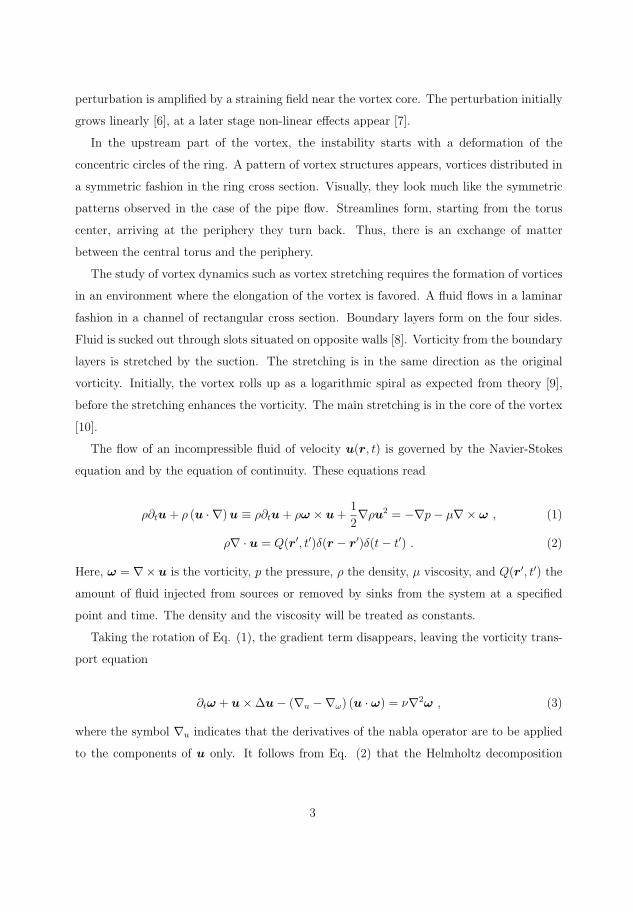
perturbation is amplified by a straining field near the vortex core. The perturbation initially

grows linearly [6], at a later stage non-linear effects appear [7].

In the upstream part of the vortex, the instability starts with a deformation of the

concentric circles of the ring. A pattern of vortex structures appears, vortices distributed in

a symmetric fashion in the ring cross section. Visually, they look much like the symmetric

patterns observed in the case of the pipe flow. Streamlines form, starting from the torus

center, arriving at the periphery they turn back. Thus, there is an exchange of matter

between the central torus and the periphery.

The study of vortex dynamics such as vortex stretching requires the formation of vortices

in an environment where the elongation of the vortex is favored. A fluid flows in a laminar

fashion in a channel of rectangular cross section. Boundary layers form on the four sides.

Fluid is sucked out through slots situated on opposite walls [8]. Vorticity from the boundary

layers is stretched by the suction. The stretching is in the same direction as the original

vorticity. Initially, the vortex rolls up as a logarithmic spiral as expected from theory [9],

before the stretching enhances the vorticity. The main stretching is in the core of the vortex

[10].

The flow of an incompressible fluid of velocity u(r, t) is governed by the Navier-Stokes

equation and by the equation of continuity. These equations read

ρ∂tu + ρ (u · ∇) u ≡ ρ∂tu + ρω × u +1

2∇ρu2 = −∇p − μ∇× ω , (1)

ρ∇ · u = Q(r′, t′)δ(r − r′)δ(t − t′) . (2)

Here, ω = ∇×u is the vorticity, p the pressure, ρ the density, μ viscosity, and Q(r′, t′) the

amount of fluid injected from sources or removed by sinks from the system at a specified

point and time. The density and the viscosity will be treated as constants.

Taking the rotation of Eq. (1), the gradient term disappears, leaving the vorticity trans-

port equation

∂tω + u × Δu − (∇u −∇ω) (u · ω) = ν∇2ω , (3)

where the symbol ∇u indicates that the derivatives of the nabla operator are to be applied

to the components of u only. It follows from Eq. (2) that the Helmholtz decomposition

3

applies, the velocity u is uniquely defined from an rotational part urot determined by a

vector potential A, and a potential part upot determined by a scalar potential φ as

u = urot + upot = ∇× A + ∇φ . (4)

The vorticity is determined from the vector potential as ω = ∇(∇ ·A)−ΔA. It is possible

to choose A such that ∇ · A = 0.

To analyze experimentally observed vortex structures as those described above, one

needs to find solutions of the flow equations representing them. A particular kind of simple

solutions is the one where non-linear terms are explicitly zero due to properties of the

solution. In finding solutions of this kind, one may be guided by the observation that

non-linear terms disappear from the vorticity equation if:

1. the velocity is parallel to the vorticity, as seen from Eq. (1), or

2. the velocity is orthogonal to the vorticity and Δu is parallel to u, as seen from Eq. (3).

The vorticity then satisfies the vector Helmholtz equation ∂tω = νΔω.

The vortex structures observed in pipe flow, as described above, are elongated, rounded

objects including vortex multipoles of finite length. This suggests finding solutions using

spherical, or possibly ellipsoidal, coordinates. Consider the vector potential V describing a

vortex centered at the point r0 and having a symmetry axis in the direction of n

V (r, t, r0 = 0, n = ez, l) = e−νtR2

[er

l(l + 1)R

rjl

( r

R

)P 0

l (θ)

+eθ

(jl−1

( r

R

)− lR

rjl

( r

R

))P 1

l (θ) + eφjl

( r

R

)P 1

l (θ)

]. (5)

Here, R gives the length scale, jl is a spherical Bessel function of index l, Pml an associated

Legendre function but with magnetic number m restricted to m = 0 or 1. The velocity and

vorticity fields derived from this vector potential possess the property that the velocity and

the vorticity are parallel, u = VR

, ω = uR

etc. Thus, this vector potential defines an exact

solution to the non-linear vorticity transport equation. Furthermore, any superposition of

vortices of this kind, with the same length scale, centered at any points and with symmetry

axes in any directions, also constitutes an exact solution to the vorticity equation. Some

4

FIG. 1: Comparison of experimentally (left) and theoretically (right) observed streak patterns.

Velocity components in the plane are indicated by arrows, the downstream component is indicated

by color coding, where black and white signifies velocities faster or slower than the parabolic profile,

respectively. Theoretical calculations are based on the assumption that the vortex structure may

be reproduced by a number of vortices, derived from the vector potential Eq. (5), aligned in

parallel. Reprinted with permission from [B. Hof, C. W. H. van Doorne, J. Westerweel, F. T. M.

Nieuwstadt, H. Faisst, B. Eckhardt, H. Wedin, R. R. Kerswell and F. Waleffe, Science 305, 1594

(2004)]. Copyright (2006) AAAS.

examples of applications of this kind will be given below. The crucial property, underpinning

the existence of vector potentials derived from Eq. (5), is the assumption that any fluid

system left undisturbed, will decay exponentially at a uniform rate. This rate is determined

by the viscosity and a universal length scale, above denoted by R.

Aligning a number of counter-rotating vortex structures, derived from Eq. (5), the pattern

of streaks and vortices observed in pipe flow [3, 4] may be reproduced. The result is presented

in Fig. 1.

To describe a diffusive vortex structure, instead of departing from Eq. (5), it is more

efficient to depart from the Green’s function of the diffusion equation and define a vector

potential centered at r0 and having a symmetry axis in the direction of n as (in spherical

coordinates)

V (r, z, t, r0 = 0, n = ez) = eze− r2

νt (4πνt)−32 . (6)

This kind of vector potential results in a flow field where the vorticity and the velocity are

orthogonal, and this flow field decays as a power of time. We position vortices derived from

Eq. (6), with the axis in the eφ-direction, at every point of the circle of radius R with the

5

0 2 4 6 8 10r �mm�

10

20

30

40

50

60Velocity across core of torus �mm�s�

5 10 15 20 25 30x �mm�

5

10

15

20

25

30

35Vorticity from center across torus core �s�1�

0.5 1 1.5 2 2.5 3 3.5 4Log k

-4.5

-4

-3.5

-3

-2.5

-2

-1.5

-1Energy spectral function Log�E�k�� for torus

FIG. 2: Experimentally determined characteristics of a vortex ring. The top frame shows the

tangential velocity as a function of the radial distance r from the center of the core. Experimental

values are from Ref. [6]. The center frame shows the vorticity as a function of x, the distance from

the symmetry axis of rotation in the symmetry plane across the center of the core at about x = 15

mm. Experimental data are from Ref. [11]. The bottom frame shows the energy spectral function

as a function of the inverse length scale k. Experimental data are from Ref. [7]. In all frames,

the full drawn curve represents the theoretical representation as derived from a vector potential

possessing the analytical structure of Eq. (7).

center at the origin and lying in the x− y plane. By carrying out an integration around this

circle, the vector potential from all these contributions may be calculated

6

A(r, t) =

∮r′=R

dφV (r, t, r0 = r′, n = eφ)

∣∣∣∣z′=0

W (φ, t) , (7)

where W is an arbitrary weight function. As our aim is not to study instabilities, we

consider only the simplest case, we put W = 1. The integration then results in a velocity

field (spherical coordinates)

u(r, t) = e−(r2−R2)

4νt (4πνt)−32

[cot θ

rI1

(rR

2νt

)er

+

(r

2νtI1

(rR

2νt

)− R

2νtI0

(rR

2νt

))eθ + 0 eφ

], (8)

where I0 and I1 are modified Bessel functions. This velocity field may now be compared to

experimental data [6]. Similarly, one may derive the vorticity and the energy spectrum from

Eq. (7) and compare to experimental findings [7, 11]. These comparisons to experiment

have been summarized in Fig. 2.

The stretched vortex structures produced by suction [8, 10] are slender objects. Exper-

imental results are most easily discussed in terms of a velocity field given in cylindrical

coordinates (r, φ, z) suitable. Stretching along the z-axis by suction at the ends causes a

vortex to have a stagnation point at z = 0. One needs to satisfy boundary conditions

ur(r = 0, z) = 0, ur(r, z = 0) �= 0, uφ(r = 0, z) = 0, uz(r = 0, z) �= 0, uz(r, z = 0) = 0 .

A possible vector potential, giving an elementary vortex structure where the vorticity and

velocity are parallel, is given by the vector potential Eq. (5) multiplied by a weight function

with vortex structures placed along the z-axis

A(r, t) =

∫dz′

∑l

cl(z′)V (r, t, r0 = z′ez, n = ez, l) , (9)

where the coefficients cl(z′) may be arbitrarily chosen. With some restrictions from the

boundary conditions, this is effectively a model with infinitely many parameters. It should

then not present any difficulties to reproduce experimental data. This indicates that it

should be investigated what constraints may be put on the coefficients of Eq. (9).

Starting from data on the circumferential velocity at different stations of z, one notices

that the maximum velocity as a function of r increases with z in the same manner as does

7

0.5 1 1.5 2 2.5 3 3.5 4r �mm�

50

100

150

200

Circumferential velocity uΦ �mm�s�

10 20 30 40 50 60z �mm�

50

100

150

200

250

300Axial velocity uz along axis �mm�s�

5 10 15 20 25r �mm�

20

40

60

80

100

120

140

Axial velocity uz cross axis �mm�s�

FIG. 3: Experimental characteristics of velocity components of a stretched vortex compared to

theoretical representations. The top frame shows the circumferential velocity uφ (cylindrical coor-

dinates) as a function of the distance r from the axis of symmetry at different distances z from the

plane of stagnation, from top to bottom z = 7, 5, 3 and 0 mm, respectively. Experimental data

are from Ref. [10]. The center frame shows the axial velocity uz (cylindrical coordinates) along

the axis of symmetry as a function of the distance z from the plane of stagnation. Experimental

data are from Ref. [8]. The bottom frame shows the axial velocity uz in the plane of stagnation as

a function of r, the distance from the axis of symmetry. Experimental data are from Ref. [8]. In

all frames, the full drawn curve represents the theoretical representation as derived from a vector

potential possessing the analytical structure of Eq. (9).

8

the axial velocity at r = 0. Available experimental data on the velocity field [8, 10] may

be reproduced, for example, by choosing the coefficients cl(z′) as polynomials in z′. The

comparison to experimental data is summarized in Fig. 3.

We have discussed properties of some kind of solutions to the non-linear vorticity trans-

port equation and how superpositions of these solutions may be used to reproduce available

experimental data on properties of vortex structures. The derivation of the solutions dis-

cussed departs from the assumption that there is a universal rate of decay of vorticity for

a fluid system. If this decay is exponential, there are solutions to the non-linear vorticity

equation having the property that the velocity and the vorticity are parallell superpositions.

If the fluid system is diffusive and decays as an inverse power of time, one may find solutions

where the velocity and the vorticity are perpendicular. The solutions discussed possess de-

grees of freedom probably sufficient to satisfy the kind of boundary conditions commonly

considered for fluid systems. However, this point needs further clarification as well as the

relation between the solutions with different dynamical properties.

[1] B. Hof, A. Juel and T. Mullin, Phys. Rev. Lett. 91, 2245 (2003).

[2] A. G. Darbyshire and T. Mullin, J. Fluid Mech. 289, 83 (1995).

[3] B. Hof, C. W. H. van Doorne, J. Westerweel and T. M. Nieuwstadt, Phys. Rev. Lett. 95, 2145

(2005).

[4] B. Hof, C. W. H. van Doorne, J. Westerweel, F. T. M. Nieuwstadt, H. Faisst, B. Eckhardt,

H. Wedin, R. R. Kerswell and F. Waleffe, Science 305, 1594 (2004).

[5] H. Faisst and B. Eckhardt, Phys. Rev. Lett. 91, 2245 (2003).

[6] A. Dazin, P. Dupont and M. Stanislas, Exp. in Fluids 40, 383 (2006).

[7] A. Dazin, P. Dupont and M. Stanislas, Exp. in Fluids 41, 401 (2006).

[8] P. Petitjeans, J. H. Robres, J. E. Wesfreid and N. Kevlahan, Euro. J. Mech. B. /Fluids 17,

549 (1998).

[9] J. C. Vassilicos and J. G. Brasseur, Phys. Rev. E 54, 467 (1996).

[10] M. Rossi, F. Bottausci, A. Maurel and P. Petitjeans, Phys. Rev. Lett. 92, (2004).

[11] M. Gharib, E. Rambod and K. Shariff, J. Fluid Mech. 360, 121 (1998).

9

Acta Wexionensia

Nedan följer en lista på skrifter publicerade i den nuvarande Acta-serien, serie III. För för-teckning av skrifter i tidigare Acta-serier, se Växjö University Press sidor på www.vxu.se

Serie III (ISSN 1404-4307) 1. Installation Växjö universitet 1999. Nytt universitet – nya professorer. 1999. ISBN 91-

7636-233-72. Tuija Virtanen & Ibolya Maricic, 2000: Perspectives on Discourse: Proceedings from

the 1999 Discourse Symposia at Växjö University. ISBN 91-7636-237-X 3. Tommy Book, 2000: Symbolskiften i det politiska landskapet – namn-heraldik-

monument. ISBN 91-7636-234-5 4. E. Wåghäll Nivre, E. Johansson & B. Westphal (red.), 2000: Text im Kontext, ISBN

91-7636-241-85. Göran Palm & Betty Rohdin, 2000: Att välja med Smålandsposten. Journalistik och

valrörelser 1982-1998. ISBN 91-7636-249-3 6. Installation Växjö universitet 2000, De nya professorerna och deras föreläsningar.

2000. ISBN 91-7636-258-2 7. Thorbjörn Nilsson, 2001: Den lokalpolitiska karriären. En socialpsykologisk studie av

tjugo kommunalråd (doktorsavhandling). ISBN 91-7636-279-5 8. Henrik Petersson, 2001: Infinite dimensional holomorphy in the ring of formal power

series. Partial differential operators (doktorsavhandling). ISBN 91-7636-282-5 9. Mats Hammarstedt, 2001: Making a living in a new country (doktorsavhandling). ISBN

91-7636-283-310. Elisabeth Wåghäll Nivre & Olle Larsson, 2001: Aspects of the European Reforma-

tion. Papers from Culture and Society in Reformation Europe, Växjö 26-27 November 1999. ISBN 91-7636-286-8

11. Olof Eriksson, 2001: Aspekter av litterär översättning. Föredrag från ett svensk-franskt översättningssymposium vid Växjö universitet 11-12 maj 2000. ISBN 91-7636-290-6.

12. Per-Olof Andersson, 2001: Den kalejdoskopiska offentligheten. Lokal press, värde-mönster och det offentliga samtalets villkor 1880-1910 (Doktorsavhandling). ISBN: 91-7636-303-1.

13. Daniel Hjorth, 2001: Rewriting Entrepreneurship. Enterprise discourse and entrepre-neurship in the case of re-organising ES (doktorsavhandling). ISBN: 91-7636-304-X.

14. Installation Växjö universitet 2001, De nya professorerna och deras föreläsningar,2001. ISBN 91-7636-305-8.

15. Martin Stigmar, 2002. Metakognition och Internet. Om gymnasieelevers informa-tionsanvändning vid arbete med Internet (doktorsavhandling). ISBN 91-7636-312-0.

16. Sune Håkansson, 2002. Räntefördelningen och dess påverkan på skogsbruket. ISBN 91-7636-316-3.

17. Magnus Forslund, 2002. Det omöjliggjorda entreprenörskapet. Om förnyelsekraft och företagsamhet på golvet (doktorsavhandling). ISBN 91-7636-320-1.

18. Peter Aronsson och Bengt Johannisson (red), 2002. Entreprenörskapets dynamik och lokala förankring. ISBN: 91-7636-323-6.

19. Olof Eriksson, 2002. Stil och översättning. ISBN: 91-7636-324-4 20. Ia Nyström, 2002. ELEVEN och LÄRANDEMILJÖN. En studie av barns lärande

med fokus på läsning och skrivning (doktorsavhandling). ISBN: 91-7636-351-1

21. Stefan Sellbjer, 2002. Real konstruktivism – ett försök till syntes av två dominerande perspektiv på undervisning och lärande (doktorsavhandling). ISBN: 91-7636-352-X

22. Harald Säll, 2002. Spiral Grain in Norway Spruce (doktorsavhandling). ISBN: 91-7636-356-2

23. Jean-Georges Plathner, 2003. La variabilité du pronom de la troisième personne en complément prépositionnel pour exprimer le réfléchi (doktorsavhandling). ISBN: 91-7636-361-9

24. Torbjörn Bredenlöw, 2003. Gestaltning – Förändring – Effektivisering. En teori om företagande och modellering. ISBN: 91-7636-364-3

25. Erik Wångmar, 2003. Från sockenkommun till storkommun. En analys av storkom-munreformens genomförande 1939-1952 i en nationell och lokal kontext (doktorsav-handling). ISBN: 91-7636-370-8

26. Jan Ekberg (red), 2003, Invandring till Sverige – orsaker och effekter. Årsbok från forskningsprofilen AMER. ISBN: 91-7636-375-9

27. Eva Larsson Ringqvist (utg.), 2003, Ordföljd och informationsstruktur i franska och svenska. ISBN: 91-7636-379-1

28. Gill Croona, 2003, ETIK och UTMANING. Om lärande av bemötande i professions-utbildning (doktorsavhandling). ISBN: 91-7636-380-5

29. Mikael Askander, 2003, Modernitet och intermedialitet i Erik Asklunds tidiga roman-konst (doktorsavhandling). ISBN: 91-7636-381-3

30. Christer Persson, 2003, Hemslöjd och folkökning. En studie av befolkningsutveck-ling, proto-industri och andra näringar ur ett regionalt perspektiv. ISBN: 91-7636-390-2

31. Hans Dahlqvist, 2003, Fri att konkurrera, skyldig att producera. En ideologikritisk granskning av SAF 1902-1948 (doktorsavhandling). ISBN: 91-7636-393-7

32. Gunilla Carlsson, 2003, Det våldsamma mötets fenomenologi – om hot och våld i psykiatrisk vård (doktorsavhandling). ISBN: 91-7636-400-3

33. Imad Alsyouf, 2004. Cost Effective Maintenance for Competitive Advantages (doktor-savhandling). ISBN: 91-7636-401-1.

34. Lars Hansson, 2004. Slakt i takt. Klassformering vid de bondekooperativa slakteriin-dustrierna i Skåne 1908-1946 (doktorsavhandling). ISBN: 91-7636-402-X.

35. Olof Eriksson, 2004. Strindberg och det franska språket. ISBN: 91-7636-403-8. 36. Staffan Stranne, 2004. Produktion och arbete i den tredje industriella revolutionen.

Tarkett i Ronneby 1970-2000 (doktorsavhandling). ISBN: 91-7636-404-6. 37. Reet Sjögren, 2004. Att vårda på uppdrag kräver visdom. En studie om vårdandet av

män som sexuellt förgripit sig på barn (doktorsavhandling). ISBN: 91-7636-405-4.

38. Maria Estling Vannestål, 2004. Syntactic variation in English quantified noun phrases with all, whole, both and half (doktorsavhandling). ISBN: 91-7636-406-2.

39. Kenneth Strömberg, 2004. Vi och dom i rörelsen. Skötsamhet som strategi och identitet bland föreningsaktivisterna i Hovmantorp kommun 1884-1930 (doktorsavhandling). ISBN: 91-7686-407-0.

40. Sune G. Dufwa, 2004. Kön, lön och karriär. Sjuksköterskeyrkets omvandling under 1900-talet (doktorsavhandling). ISBN: 91-7636-408-9

41. Thomas Biro, 2004. Electromagnetic Wave Modelling on Waveguide Bends, Power Lines and Space Plasmas (doktorsavhandling). ISBN: 91-7636-410-0

42. Magnus Nilsson, 2004, Mångtydigheternas klarhet. Om ironier hos Torgny Lindgren från Skolbagateller till Hummelhonung (doktorsavhandling). ISBN:91-7636-413-5

43. Tom Bryder, 2004. Essays on the Policy Sciences and the Psychology of Politics and Propaganda. ISBN: 91-7636-414-3

44. Lars-Göran Aidemark, 2004. Sjukvård i bolagsform. En studie av Helsingborgs Lasa-rett AB och Ängelholms Sjukhus AB. ISBN: 91-7636-417-8

45. Per-Anders Svensson, 2004. Dynamical Systems in Local Fields of Characteristic Zero (doktorsavhandling). ISBN: 91-7636-418-6

46. Rolf G Larsson, 2004. Prototyping inom ABC och BSc. Erfarenheter från aktions-forskning i tre organisationer (doktorsavhandling). ISBN: 91-7636-420-8

47. Päivi Turunen, 2004. Samhällsarbete i Norden. Diskurser och praktiker i omvandling (doktorsavhandling). ISBN: 91-7636-422-4

48. Carina Henriksson, 2004. Living Away from Blessings. School Failure as Lived Ex-perience (doktorsavhandling). ISBN: 91-7636-425-9

49. Anne Haglund, 2004. The EU Presidency and the Northern Dimension Initiative: Ap-plying International Regime Theory (doktorsavhandling). ISBN: 91-7636-428-3

50. Ulla Rosén, 2004. Gamla plikter och nya krav. En studie om egendom, kvinnosyn och äldreomsorg i det svenska agrarsamhället 1815-1939. ISBN: 91-7636-429-1

51. Michael Strand, 2004. Particle Formation and Emission in Moving Grate Boilers Op-erating on Woody Biofuels (doktorsavhandling). ISBN: 91-7636-430-5

52. Bengt-Åke Gustafsson, 2004. Närmiljö som lärmiljö – betraktelser från Gnosjöregionen. ISBN: 91-7636-432-1

53. Lena Fritzén (red), 2004. På väg mot integrativ didaktik. ISBN: 91-7636-433-X 54. M.D. Lyberg, T. Lundström & V. Lindberg, 2004. Physics Education. A short history. Con-

temporary interdisciplinary research. Some projects. ISBN: 91-7636-435-6 55. Gunnar Olofsson (red.), 2004. Invandring och integration. Sju uppsatser från forsk-

ningsmiljön ”Arbetsmarknad, Migration och Etniska relationer” (AMER) vid Växjö universitet. ISBN: 91-7636-437-2

56. Malin Thor, 2005. Hechaluz – en rörelse i tid och rum. Tysk-judiska ungdomars exil i Sverige 1933-1943 (doktorsavhandling). ISBN: 91-7636-438-0

57. Ibolya Maricic, 2005. Face in cyberspace: Facework, (im)politeness and conflict in English discussion groups (doktorsavhandling). ISBN: 91-7636-444-5

58. Eva Larsson Ringqvist och Ingela Valfridsson (red.), 2005. Forskning om undervis-ning i främmande språk. Rapport från workshop i Växjö 10-11 juni 2004. ISBN: 91-7636-450-X

59. Vanja Lindberg, 2005. Electronic Structure and Reactivity of Adsorbed Metallic Quantum Dots (doktorsavhandling). ISBN: 91-7636-451-8

60. Lena Agevall, 2005. Välfärdens organisering och demokratin – en analys av New Pub-lic Management. ISBN: 91-7636-454-2

61. Daniel Sundberg, 2005. Skolreformernas dilemman – En läroplansteoretisk studie av kampen om tid i den svenska obligatoriska skolan (doktorsavhandling). ISBN: 91-7636-456-9.

62. Marcus Nilsson, 2005. Monomial Dynamical Systems in the Field of p-adic Numbers and Their Finite Extensions (doktorsavhandling). ISBN: 91-7636- 458-5.

63. Ann Erlandsson, 2005. Det följdriktiga flockbeteendet: en studie om profilering på ar-betsmarknaden (doktorsavhandling). ISBN: 91-7636-459-3.

64. Birgitta Sundström Wireklint, 2005. Förberedd på att vara oförberedd. En feno-menologisk studie av vårdande bedömning och dess lärande i ambulanssjukvård (dok-torsavhandling). ISBN: 91-7636-460-7

65. Maria Nilsson, 2005. Differences and similarities in work absence behavior – empiri-cal evidence from micro data (doktorsavhandling). ISBN: 91-7636-462-3

66. Mikael Bergström och Åsa Blom, 2005. Above ground durability of Swedish softwood (doktorsavhandling). ISBN: 91-7636-463-1

67. Denis Frank, 2005. Staten, företagen och arbetskraftsinvandringen - en studie av in-vandringspolitiken i Sverige och rekryteringen av utländska arbetare 1960-1972 (doktors-avhandling). ISBN: 91-7636-464-X

68. Mårten Bjellerup, 2005. Essays on consumption: Aggregation, Asymmetry and Asset Dis-tributions (doktorsavhandling). ISBN: 91-7636-465-8.

69. Ragnar Jonsson, 2005. Studies on the competitiveness of wood – market segmentation and customer needs assessment (doktorsavhandling). ISBN: 91-7636-468-2.

69. Anders Pehrsson och Basim Al-Najjar, Creation of Industrial Competitiveness: CIC 2001-2004. ISBN: 91-7646-467-4.

70. Ali M. Ahmed, 2005. Essays on the Behavioral Economics of Discrimination (doktors-avhandling). ISBN: 91-7636-472-0.

71. Katarina Friberg, 2005. The workings of co-operation.. A comparative study of con-sumer co-operative organisation in Britain and Sweden, 1860 to 1970 (doktorsavhan-dling). ISBN: 91-7636-470-4.

72. Jonas Sjölander, 2005. Solidaritetens omvägar. Facklig internationalism i den tredje indust-riella revolutionen – (LM) Ericsson, svenska Metall och Ericssonarbetarna i Colombia 1973-1993 (doktorsavhandling) ISBN: 91-7636-474-7.

73. Daniel Silander, 2005. Democracy from the outside-in? The conceptualization and signifi-cance of democracy promotion (doktorsavhandling). ISBN: 91-7636-475-5.

74. Serge de Gosson de Varennes, 2005. Multi-oriented Symplectic Geometry and the Exten-sion of Path Intersection Indices (doktorsavhandling). ISBN: 91-7636-477-1.

75. Rebecka Ulfgard, 2005. Norm Consolidation in the European Union: The EU14-Austria Crisis in 2000 (doktorsavhandling). ISBN: 91-7636-482-8

76. Martin Nilsson, 2005. Demokratisering i Latinamerika under 1900-talet – vänstern och de-mokratins fördjupning (doktorsavhandling). ISBN: 91-7636-483-6

77. Thomas Panas, 2005. A Framework for Reverse Engineering (doktorsavhandling). ISBN: 91-7636-485-2

78. Susanne Linnér, 2005. Värden och villkor – pedagogers samtal om ett yrkesetiskt doku-ment (doktorsavhandling). ISBN: 91-7636-484-4.

79. Lars Olsson (red), 2005. Invandring, invandrare och etniska relationer I Sverige 1945-2005. Årsbok från forskningsmiljön AMER vid Växjö universitet. ISBN: 91-7636-488-7.

80. Johan Svanberg, 2005. Minnen av migrationen. Arbetskraftsinvandring från Jugoslavien till Svenska Fläktfabriken i Växjö kring 1970. ISBN: 91-7636-490-9.

81. Christian Ackrén, 2006. On a problem related to waves on a circular cylinder with a surface impedance (licentiatavhandling). ISBN: 91-7636-492-5.

82. Stefan Lund, 2006. Marknad och medborgare – elevers valhandlingar i gymnasieutbildningens integrations- och differentieringsprocesser (doktorsavhandling). ISBN: 91-7636-493-3.

83. Ulf Petäjä, 2006. Varför yttrandefrihet? Om rättfärdigandet av yttrandefrihet med utgångs-punkt från fem centrala argument i den demokratiska idétraditionen (doktorsavhandling). ISBN: 91-7636-494-1.

84. Lena Carlsson, 2006. Medborgarskap som demokratins praktiska uttryck i skolan – diskursiva konstruktioner av gymnasieskolans elever som medborgare (doktorsavhandling). ISBN: 91-7636-495-X

85. Åsa Gustafsson, 2006. Customers logistics service requirements and logistics strategies in the Swedish sawmill industry (doktorsavhandling). ISBN: 91-7636-498-4.

86. Kristina Jansson, 2006. Saisir l’insaisissable. Les formes et les traductions du discours indirect libre dans des romans suédois et français (doktorsavhandling). ISBN: 91-7636-499-2

87. Edith Feistner, Alfred Holl, 2006. Mono-perspective views of multi-perspectivity : In-formation systems modeling and ‘The bild men and the elephant’. ISBN : 91-7636-500-X.

88. Katarina Rupar-Gadd, 2006. Biomass Pre-treatment for the Production of Sustainable Energy – Emissions and Self-ignition (doktorsavhandling). ISBN: 91-7636-501-8.

89. Lena Agevall, Håkan Jenner (red.),2006. Bilder av polisarbete – Samhällsuppdrag, dilemman och kunskapskrav. ISBN: 91-7636-502-6

90. Maud Ihrskog, 2006. Kompisar och Kamrater .Barns och ungas villkor för relationsskapande i vardagen (doktorsavhandling). ISBN: 91-7636-503-4.

91. Detlef Quast, 2006. Die Kunst die Zukunft zu erfinden Selbstrationalität, asymmetrische Information und Selbstorganisation in einer wissensintensiven professionellen Non Profit Organisation. Eine informationstheoretische und organisationssoziologische Studie zum Verständnis des Verhaltens der Bibliotheksverwaltung (doktorsavhandling). ISBN: 91-7636-505-0.

92. Ulla Johansson, 2006. Design som utvecklingskraft. En utvärdering av regeringens designsatsning 2003-2005. ISBN: 91-7636-507-7.

93. Klara Helstad, 2006. Managing timber procurement in Nordic purchasing sawmills (doktorsavhandling). ISBN:91-7636-508-5.

94. Göran Andersson, Rolf G. Larsson, 2006. Boundless value creation. Strategic man-agement accounting in value system configuration. ISBN: 91-7636-509-3.

95. Jan Håkansson, 2006. Lärande mellan policy och praktik. Kontextuella villkor för skolans reformarbete (doktorsavhandling). ISBN: 91-7636-510-7.

96. Frederic Bill, 2006. The Apocalypse of Entrepreneurship (doktorsavhandling). ISBN: 91-7636-513-1.

97. Lena Fritzén, 2006. “On the edge” – om förbättringsledarskap i hälso- och sjukvård ISBN: 91-7636-516-6

98. Marianne Lundgren, 2006. Från barn till elev i riskzon. En analys av skolan som kategoriseringsarena (doktorsavhandling). ISBN: 91-7636-518-2.

99. Mari Mossberg, 2006, La relation de concession. Étude contrastive de quelques con-necteurs concessifs français et suédois (doktorsavhandling). ISBN : 91-7636-517-4.

100. Leif Grönqvist, 2006. Exploring Latent Semantic Vector Models Enriched With N-grams (doktorsavhandling), ISBN: 91-7636-519-0.

101. Katarina Hjelm (red), 2006. Flervetenskapliga perspektiv i migrationsforskning. Årsbok 2006 från forskningsprofilen Arbetsmarknad, Migration och Etniska relationer (AMER) vid Växjö universitet. ISBN: 91-7636-520-4.

102. Susanne Thulin, 2006. Vad händer med lärandets objekt? En studie av hur lärare och barn i förskolan kommunicerar naturvetenskapliga fenomen (licentiatavhandling), ISBN: 91-7636-521-2

103. Per Nilsson, 2006. Exploring Probabilistic Reasoning – A Study of How Students Contextualise Compound Chance Encounters in Explorative Settings (doktorsav-handling), ISBN: 91-7636-522-0.

104. PG Fahlström, Magnus Forslund, Tobias Stark (red.), 2006, Inkast. Idrottsforskning vid Växjö universitet. ISBN: 91-7636-523-9.

105. Ulla Johansson (red.), 2006, Design som utvecklingskraft II. Fem uppsatser om Fem uppsatser om utvalda projekt från regeringens designsatsning 2003-2005, ISBN: 91-7636-530-1.

106. Ann-Charlotte Larsson 2007, Study of Catalyst Deactivation in Three Different In-dustrial Processes (doktorsavhandling), ISBN: 978-91-7636-533-5.

107. Karl Loxbo, 2007,Bakom socialdemokraternas beslut. En studie av den politiska förändringens dilemman - från 1950-talets ATP-strid till 1990-talets pensionsuppgörel-se (doktorsavhandling), ISBN: 978-91-7636-535-9.

108. Åsa Nilsson-Skåve, 2007,Hjärtat som hör det förstummade spela. Studier i Stina Aronsons berättarkonst (doktorsavhandling), ISBN: 978-91-7636-536-6.

109. Anne Haglund Morrissey, Daniel Silander (eds.), 2007, The EU and the Outside World - Global Themes in a European Setting, ISBN: 978-91-7636-537-3.

110. Robert Nyqvist, 2007, Algebraic Dynamical Systems, Analytical Results and Nume-rical Simulations (doktorsavhandling), ISBN: 978-91-7636-547-2.

111. Christer Fritzell, Lena Fritzén, 2007, Integrativ didaktik i olika ämnesperspektiv. ISBN: 978-91-7636-548-9.

112. Torgny Klasson, Daniel Silander, 2007. Hot och hotbilder i globaliseringens tid – en studie av den svenska säkerhetspolitiska debatten. ISBN: 978-91-7636-550-2

113. Olof Eriksson (red.), 2007. Översättning och Kultur. Föredrag från ett symposium vid Växjö universitet 17-18 november 2006, ISBN: 978-91-7636-552-6

114. Henrik Tryggeson, 2007. Analytical Vortex Solutions to Navier-Stokes Equation (doktorsavhandling), ISBN: 978-91-7636-555-7.

Växjö University Press 351 95 Växjö www.vxu.se vup@vxu.se