analyzing changes in software systems from changedistiller to fmdiff
TRANSCRIPT

Analyzing Changes in Software Systems From ChangeDistiller to FMDiff
Martin Pinzger Software Engineering Research Group University of Klagenfurt http://serg.aau.at/bin/view/MartinPinzger

Kartendaten © 2014 Basarsoft, GeoBasis-DE/BKG (©2009), Google 100 km
Google Maps https://www.google.at/maps/preview
1 of 1 28/06/14 11:17
Pfunds
PhD
Postdoc
Assistant Professor
Univ. Prof.

Software systems change [Lehman et al.]
Views on Mozilla evolution 50% of files have been modified in last quarter of observation
3

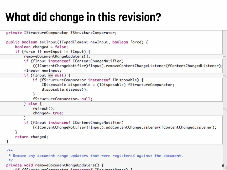
What did change in this revision?
5

What is the impact of these changes?
6

Do these changes affect my code?
7

Understanding changes and their impact
Current tools lack support for comprehending changes “How do software engineers understand code changes? - an exploratory study in industry”, Tao et al. 2012
Developers need to reconstruct the detailed context and impact of each change which is time consuming and error prone
“An exploratory study of awareness interests about software modifications”, Kim 2011
8

We need better support to analyze and comprehend changes and their impact

Overview of (my) tools
ChangeDistiller Fine-Grained Evolution of Java classes
WSDLDiff Evolution of service-oriented systems
FMDiff Evolution of feature models
10

ChangeDistiller Fine-grained evolution of Java classes
Beat Fluri, Martin Pinzger, and Harald Gall
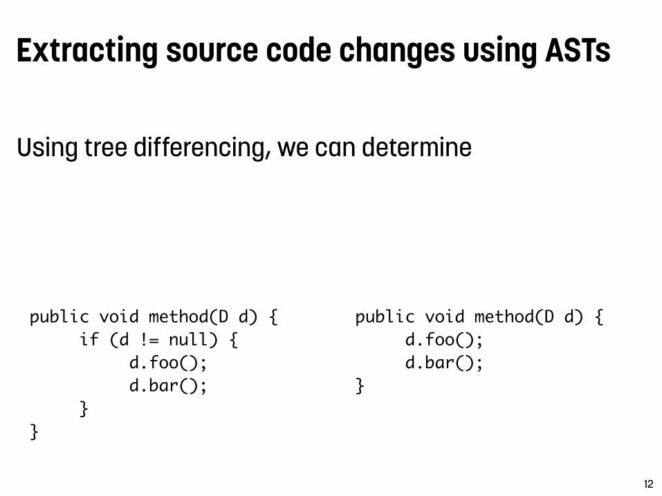
Extracting source code changes using ASTs
Using tree differencing, we can determine
public void method(D d) {if (d != null) {
d.foo();d.bar();
}}
public void method(D d) {d.foo();d.bar();
}
12

Using tree differencing, we can determine Enclosing entity (root node)
Extracting source code changes using ASTs
public void method(D d) {if (d != null) {
d.foo();d.bar();
}}
public void method(D d) {d.foo();d.bar();
}
13
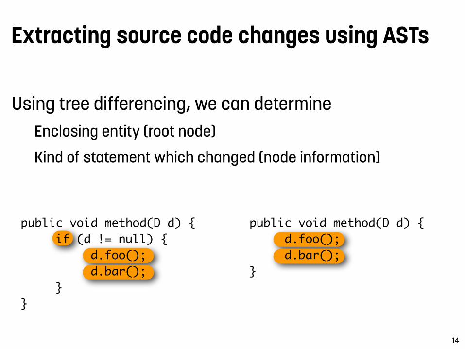
Using tree differencing, we can determine Enclosing entity (root node)
Kind of statement which changed (node information)
public void method(D d) {d.foo();d.bar();
}
public void method(D d) {if (d != null) {
d.foo();d.bar();
}}
Extracting source code changes using ASTs
14

Using tree differencing, we can determine Enclosing entity (root node)
Kind of statement which changed (node information)
Kind of change (tree edit operation)
public void method(D d) {if (d != null) {
d.foo();d.bar();
}}
public void method(D d) {d.foo();d.bar();
}
Extracting source code changes using ASTs
15
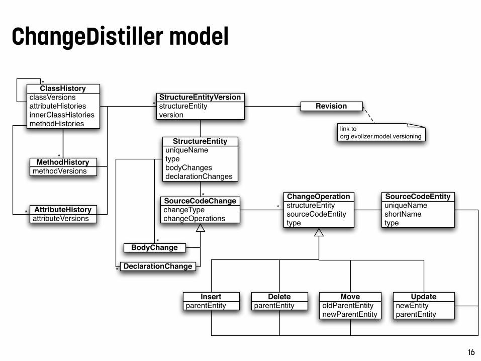
ChangeDistiller model
uniqueNameshortNametype
SourceCodeEntitystructureEntitysourceCodeEntitytype
ChangeOperation
parentEntityInsert
parentEntityDelete
oldParentEntitynewParentEntity
MovenewEntityparentEntity
Update
uniqueNametypebodyChangesdeclarationChanges
StructureEntity
*
changeTypechangeOperations
SourceCodeChange*
structureEntityversion
StructureEntityVersion
attributeVersionsAttributeHistory
methodVersionsMethodHistory
*classVersionsattributeHistoriesinnerClassHistoriesmethodHistories
ClassHistory
*
*
*
Revision
link to
org.evolizer.model.versioning
BodyChange
DeclarationChange*
*
16

ChangeDistiller tool
Dem
17https://bitbucket.org/sealuzh/tools-changedistiller/wiki/Home
ChangeDistiller references
“Change distilling: Tree differencing for fine-grained source code change extraction”, Fluri et al. 2007
Diffing UML diagrams “UMLDiff: An Algorithm for Object-Oriented Design Differencing”, Xing et al. 2005
Recording changes in the IDE “Mining Fine-grained Code Changes to Detect Unknown Change Patterns”, Negara et al. 2014
18

ChangeDistiller improved -> gumtree
gumtree (sources available at GitHub) “Fine-grained and accurate source code differencing”, Falleri et al. 2014
19
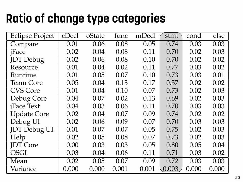
Ratio of change type categories
Table 2: Categories of fine-grained source code changesCategory Description
cDeclAggregates all changes that alter the declaration of a class:Modifier changes, class renaming, class API changes, par-ent class changes, and changes in the ”implements list”.
oState Aggregates the insertion and deletion of object states of aclass, i.e., adding and removing fields.
func Aggregates the insertion and deletion of functionality of aclass, i.e., adding and removing methods.
mDecl
Aggregates all changes that alter the declaration of amethod: Modifier changes, method renaming, method APIchanges, return type changes, and changes of the parame-ter list.
stmt Aggregates all changes that modify executable statements,e.g., insertion or deletion of statements.
cond Aggregates all changes that alter condition expressions incontrol structures.
else Aggregates the insertion and deletion of else-parts.
Table 3: Relative frequencies of SCC categories per Eclipseproject, plus their mean and variance over all selectedprojects.
Eclipse Project cDecl oState func mDecl stmt cond elseCompare 0.01 0.06 0.08 0.05 0.74 0.03 0.03jFace 0.02 0.04 0.08 0.11 0.70 0.02 0.03JDT Debug 0.02 0.06 0.08 0.10 0.70 0.02 0.02Resource 0.01 0.04 0.02 0.11 0.77 0.03 0.02Runtime 0.01 0.05 0.07 0.10 0.73 0.03 0.01Team Core 0.05 0.04 0.13 0.17 0.57 0.02 0.02CVS Core 0.01 0.04 0.10 0.07 0.73 0.02 0.03Debug Core 0.04 0.07 0.02 0.13 0.69 0.02 0.03jFace Text 0.04 0.03 0.06 0.11 0.70 0.03 0.03Update Core 0.02 0.04 0.07 0.09 0.74 0.02 0.02Debug UI 0.02 0.06 0.09 0.07 0.70 0.03 0.03JDT Debug UI 0.01 0.07 0.07 0.05 0.75 0.02 0.03Help 0.02 0.05 0.08 0.07 0.73 0.02 0.03JDT Core 0.00 0.03 0.03 0.05 0.80 0.05 0.04OSGI 0.03 0.04 0.06 0.11 0.71 0.03 0.02Mean 0.02 0.05 0.07 0.09 0.72 0.03 0.03Variance 0.000 0.000 0.001 0.001 0.003 0.000 0.000
Some change types defined in [11] such as the ones thatchange the declaration of an attribute are left out in our anal-ysis as their total frequency is below 0.8%. The complete listof all change types, their meanings and their contexts can befound in [11].
Table 3 shows the relative frequencies of each category ofSCC per Eclipse project, plus their mean and variance overall selected projects. Looking at the mean values listed inthe second last row of the table, we can see that 70% of allchanges are stmt changes. These are relatively small changesand affect only single statements. Changes that affect the ex-isting control flow structures, i.e., cond and else, constituteonly about 6% on average. While these changes might af-fect the behavior of the code, their impact is locally limitedto their proximate context and blocks. They ideally do not in-duce changes at other locations in the source code. cDecl, oS-tate, func, and mDecl represent about one fourth of all changesin total. They change the interface of a class or a methodand do—except when adding a field or a method—require achange in the dependent classes and methods. The impactof these changes is according to the given access modifiers;within the same class or package (private or default) orexternal code (protected or public).
The values in Table 3 show small variances and relativelynarrow confidence intervals among the categories across all
Table 4: Spearman rank correlation between SCC cate-gories (*marks significant correlations at � = 0.01.)
cDecl oState func mDecl stmt cond elsecDecl 1.00� 0.33� 0.42� 0.49� 0.23� 0.21� 0.21�oState 1.00� 0.65� 0.53� 0.62� 0.51� 0.51�func 1.00� 0.67� 0.66� 0.53� 0.53�mDecl 1.00� 0.59� 0.49� 0.48�stmt 1.00� 0.71� 0.7�cond 1.00� 0.67�else 1.00�
projects. This is an interesting observation as these Eclipseprojects do vary in terms of file size and changes (see Table 1).
3.2 Correlation of SCC CategoriesWe first performed a correlation analysis between the dif-
ferent SCC categories of all source files of the selected projects.We use the Spearman rank correlation because it makes noassumptions about the distributions, variances and the typeof relationship. It compares the ordered ranks of the vari-ables to measure a monotonic relationship. This makes Spear-man more robust than Pearson correlation, which is restrictedto measure the strength of a linear association between twonormal distributed variables [8]. Spearman values of +1 and-1 indicate a high positive or negative correlation, whereas 0tells that the variables do not correlate at all. Values greaterthan +0.5 and lower than -0.5 are considered to be substan-tial; values greater than +0.7 and lower than -0.7 are consid-ered to be strong correlations [31].
Table 4 lists the results. Some facts can be read from thevalues: cDecl does neither have substantial nor strong cor-relation with any of the other change types. oState has itshighest correlation with func. func has approximately equalhigh correlations with oState, mDecl, and stmt. The strongestcorrelations are between stmt, cond, and else with 0.71, 0.7,and 0.67.
While this correlation analysis helps to gain knowledgeabout the nature and relation of change type categories itmainly reveals multicollinearity between those categories thatwe have to address when building regression models. Acausal interpretation of the correlation values is tedious andmust be dealt with caution. Some correlations make senseand could be explained using common knowledge about pro-gramming. For instance, the strong correlations between stmt,cond, and else can be explained that often local variables areaffected when existing control structures are changed. Thisis because they might are moved into a new else-part or be-cause a new local variable is needed to handle the differentconditions. In [12], Fluri et al. attempt to find an expla-nation why certain change types occur more frequently to-gether than others, i.e., why they correlate.
3.3 Correlation of Bugs, LM, and SCCH 1 formulated in Section 1 aims at analyzing the correla-
tion between Bugs, LM, and SCC (on the level of source files).It serves two purposes: (1) We analyze whether there is a sig-nificant correlation between SCC and Bugs. A significant cor-relation is a precondition for any further analysis and predic-tion model. (2) Prior work reported on the positive relationbetween Bugs an LM. We explore the extent to which SCChas a stronger correlation with Bugs than LM. We apply theSpearman rank correlation to each selected Eclipse project toinvestigate H 1.
20

Predicting bug-prone files
Figure 2: Scatterplot between the number of bugs andnumber of SCC on file level. Data points were obtainedfor the entire project history.
3.5 Predicting Bug- & Not Bug-Prone FilesThe goal of H 3 is to analyze if SCC can be used to dis-
criminate between bug-prone and not bug-prone files in ourdataset. We build models based on different learning tech-niques. Prior work states some learners perform better thanothers. For instance Lessman et al. found out with an ex-tended set of various learners that Random Forest performsthe best on a subset of the NASA Metrics dataset. But in re-turn they state as well that performance differences betweenlearners are marginal and not significant [20].
We used the following classification learners: Logistic Re-gression (LogReg), J48 (C 4.5 Decision Tree), RandomForest (Rnd-For), Bayesian Network (B-Net) implemented by the WEKAtoolkit [36], Exhaustive CHAID a Decision Tree based on chisquared criterion by SPSS 18.0, Support Vector Machine (Lib-SVM [7]), Naive Bayes Network (N-Bayes) and Neural Nets (NN)both provided by the Rapid Miner toolkit [24]. The classifierscalculate and assign a probability to a file if it is bug-prone ornot bug-prone.
For each Eclipse project we binned files into bug-prone andnot bug-prone using the median of the number of bugs per file(#bugs):
bugClass =
⇢not bug � prone : #bugs <= median
bug � prone : #bugs > median
When using the median as cut point the labeling of a file isrelative to how much bugs other files have in a project. Thereexist several ways of binning files afore. They mainly vary inthat they result in different prior probabilities: For instanceZimmerman et al. [40] and Bernstein et al. [4] labeled files asbug-prone if they had at least one bug. When having heavilyskewed distributions this approach may lead to high a priorprobability towards a one class. Nagappan et al. [28] used astatistical lower confidence bound. The different prior prob-abilities make the use of accuracy as a performance measurefor classification difficult.
As proposed in [20, 23] we therefore use the area underthe receiver operating characteristic curve (AUC) as perfor-mance measure. AUC is independent of prior probabilitiesand therefore a robust measure to asses the performance andaccuracy of predictor models [4]. AUC can be seen as theprobability, that, when choosing randomly a bug-prone and
Table 6: AUC values of E 1 using logistic regression withLM and SCC as predictors for bug-prone and a not bug-
prone files. Larger values are printed in bold.Eclipse Project AUC LM AUC SCCCompare 0.84 0.85jFace 0.90 0.90JDT Debug 0.83 0.95Resource 0.87 0.93Runtime 0.83 0.91Team Core 0.62 0.87CVS Core 0.80 0.90Debug Core 0.86 0.94jFace Text 0.87 0.87Update Core 0.78 0.85Debug UI 0.85 0.93JDT Debug UI 0.90 0.91Help 0.75 0.70JDT Core 0.86 0.87OSGI 0.88 0.88Median 0.85 0.90Overall 0.85 0.89
a not bug-prone file the trained model then assigns a higherscore to the bug-prone file [16].
We performed two bug-prone vs. not bug-prone classifica-tion experiments: In experiment 1 (E 1) we used logistic re-gression once with total number of LM and once with totalnumber of SCC as predictors. E 1 investigates H 3–SCC canbe used to discriminate between bug- and not bug-prone files–and in addition whether SCC is a better predictor than codechurn based on LM .
Secondly in experiment 2 (E 2) we used the above men-tioned classifiers and the number of each category of SCCdefined in Section 3.1 as predictors. E 2 investigates whetherchange types are good predictors and if the additional typeinformation yields better results than E 1 where the type of achange is neglected. In the following we discuss the resultsof both experiments:Experiment 1: Table 6 lists the AUC values of E 1 for eachproject in our dataset. The models were trained using 10 foldcross validation and the AUC values were computed whenreapplying a learned model on the dataset it was obtainedfrom. Overall denotes the model that was learned when merg-ing all files of the projects into one larger dataset. SCC achievesa very good performance with a median of 0.90–more thanhalf of the projects have AUC values equal or higher than0.90. This means that logistic regression using SCC as predic-tor ranks bug-prone files higher than not bug-prone ones witha probability of 90%. Even Help having the lowest value isstill within the range of 0.7 what Lessman et al. call ”promis-ing results” [20]. This low value is accompanied with thesmallest correlation of 0.48 of SCC in Table 4. The good per-formance of logistic regression and SCC is confirmed by anAUC value of 0.89 when learning from the entire dataset.With a value of 0.004 AUCSCChas a low variance over allprojects indicating consistent models. Based on the results ofE 1 we accept H 3—SCC can be used to discriminate betweenbug- and not bug-prone files.
With a median of 0.85 LM shows a lower performance thanSCC . Help is the only case where LM is a better predictorthan SCC . This not surprising as it is the project that yieldsthe largest difference in favor of LM in Table 4. In general thecorrelation values in Table 4 reflect the picture given by theAUC values. For instance jFace Text and JDT Debug UI thatexhibit similar correlations performed nearly equal. A Re-
21
SCC outperforms LM
“Comparing Fine-Grained Source Code Changes And Code Churn For Bug Prediction”, Giger et al. 2011
More info:
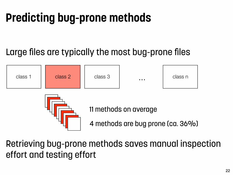
Predicting bug-prone methods
Large files are typically the most bug-prone files
Retrieving bug-prone methods saves manual inspection effort and testing effort
11 methods on average
class 1 class 2 class 3 class n...class 2
4 methods are bug prone (ca. 36%)
22

Predicting bug-prone methods
Models computed with change metrics (CM) perform best authors and methodHistories are the most important measures
More info “Method-Level Bug Prediction”, Giger et al. 2012
23
Table 4: Median classification results over all pro-jects per classifier and per model
CM SCM CM&SCM
AUC P R AUC P R AUC P R
RndFor .95 .84 .88 .72 .5 .64 .95 .85 .95
SVM .96 .83 .86 .7 .48 .63 .95 .8 .96
BN .96 .82 .86 .73 .46 .73 .96 .81 .96
J48 .95 .84 .82 .69 .56 .58 .91 .83 .89
values of the code metrics model are approximately 0.7 foreach classifier—what is defined by Lessman et al. as ”promis-ing” [26]. However, the source code metrics suffer from con-siderably low precision values. The highest median precisionvalue for the code metrics model is obtained in case of J48(0.56). For the remaining classifiers the values are around 0.5.In other words, using the code metrics half of the methodsare correctly classified (the other half being false positives).Moreover, code metrics only achieve moderate median recallvalues close to 0.6 (except for NB), i.e., only two third of allbug-prone methods are retrieved.Second, the change metrics and the combined model per-
form almost equally. Moreover, both exhibit good values incase of all three performance measures (refers to RQ1 intro-duced in Section 1). Only the median recall values obtainedby SVM and BN for the combined model are significantlyhigher than the ones of the change metrics model (0.96 vs.0.86 in both cases). Moreover, while AUC and precision arefairly similar for these two models, recall seems to benefit themost from using both metric sets in combination comparedto change metrics only.Summarizing, we can say that change metrics significantly
outperform code metrics when discriminating between bug-prone and not bug-prone methods (refers to RQ2). A lookat the J48 tree models of the combined metrics set supportsthis fact as the code metrics are added towards the leaves ofthe tree, whereas except for three projects (˜14%) authorsis selected as root attribute. methodHistories is for 11 pro-jects (˜52%) the second attribute and in one case the root.Furthermore, considering the average prior probabilities inthe dataset (i.e., ˜32% of all methods are bug-prone), changemetrics perform significantly better than chance. Hence, theresults of our study confirms existing observations that his-torical change measures are good bug predictors, e.g., [17,30, 20, 24]. When using a combined model we might ex-pect slightly better recall values. However, from a strictstatistical point of view it is not necessary to collect codemeasures in addition to change metrics when predicting bug-prone methods.Regarding the four classifiers, our results are mostly con-
sistent. In particular, the performance differences betweenthe classifiers when based on the change and the combinedmodel are negligible. The largest variance in performanceamong the classifiers resulted from using the code metricsfor model building. However, in this case these results arenot conclusive: On the one hand, BN achieved significantlylower precision (median of 0.46) than the other classifiers.On the other hand, BN showed a significantly higher recallvalue (median of 0.73).
3.3 Prediction with Different Labeling PointsSo far we used the absence and presence of bugs to label a
method as not bug-prone or bug-prone, respectively. Approx-imately one third of all methods are labeled as bug-prone inour dataset (see Section 3.1). Given this number a developerwould need to spend a significant amount of her time for cor-rective maintenance activities when investigating all meth-ods being predicted as bug-prone. We analyze in this section,how the classification performance varies (RQ3) as the num-ber of samples in the target class shrinks, and whether weobserve similar findings as in Section 3.2 regarding the re-sults of the change and code metrics (RQ2). For that, weapplied three additional cut-point values as follows:
bugClass =
!
not bug − prone : #bugs <= pbug − prone : #bugs > p
(2)
where p represents either the value of the 75%, 90%, or 95%percentile of the distribution of the number of bugs in meth-ods per project. For example, using the 95% percentile ascut-point for prior binning would mean to predict the ”top-five percent” methods in terms of the number of bugs.
To conduct this study we applied the same experimentalsetup as in Section 3.1, except for the differently chosen cut-points. We limited the set of machine learning algorithms toone algorithm as we could not observe any major differencein the previous experiment among them (see Table 4). Wechose Random Forest (RndFor) for this experiment since itsperformance lied approximately in the middle of all classi-fiers.
Table 5 shows the median classification results over allprojects based on the RndFor classifier per cut-point andper metric set model. The cell coloring has the same inter-pretation as in Table 4: Grey shaded cells are significantlydifferent from the white cells of the same performance mea-sure in the same row (i.e., percentile). For better readabilityand comparability, the first row of Table 5 (denoted by GT0,i.e., greater than 0, see Equation 1) corresponds to the firstrow of Table 4 (i.e., performance vector of RndFor).
We can see that the relative performances between themetric sets behave similarly to what was observed in Sec-tion 3.2. The change (CM) and the combined (CM&SCM)models outperform the source code metrics (SCM) model sig-nificantly across all thresholds and performance measures.The combined model, however, does not achieve a signifi-cantly different performance compared to the change model.While the results in Section 3.2 showed an increase regard-ing recall in favor of the combined model, one can noticean improved precision by 0.06 in case of the 90% and the95% percentile between the change and combined model—although not statistically significant. In case of the 75% per-centile the change and the combined model achieve nearlyequal classification performance.
Comparing the classification results across the four cut-points we can see that the AUC values remain fairly constanton a high level for the change metrics and the combinedmodel. Hence, the choice of a different binning cut-pointdoes not affect the AUC values for these models. In contrast,a greater variance of the AUC values is obtained in the caseof the classification models based on the code metric set.For instance, the median AUC value when using GT0 forbinning (0.72) is significantly lower than the median AUCvalues of all other percentiles.
Generally, precision decreases as the number of samplesin the target class becomes smaller (i.e., the higher the per-centile). For instance, the code model exhibits low preci-

Research opportunities
Extract details on statement changes (-> solved by gumtree?)
Argument changes in method invocations
Nesting of statements
Expression changes Extract context information
Consider call, access, inheritance, and type dependencies
Combine with task context - see, e.g., Mylyn [Kersten and Murphy, 2005]
24
Research opportunities (cont.)
Support multiple programming languages Currently only Java is supported
Extract changes from “other” source files Configuration files, project and build files, etc.
Extract changes of whole software ecosystems
25

WSDLDiff Evolution of service-oriented systems
Daniele Romano and Martin Pinzger

Service-oriented systems
Services as contracts -> they should be stable Analyze changes to quantify the risk of using a service
27

WSDL example
28
<definitions name=“HelloService" targetNamespace="http://www.examples.com/wsdl/HelloService.wsdl" …> <message name="SayHelloRequest"> <part name="parameters" type=“ns:PersonName"/> </message> <portType name="Hello_PortType"> <operation name="sayHello"> <input message="tns:SayHelloRequest"/> <output message="tns:SayHelloResponse"/> </operation> </portType> <binding name="Hello_Binding" type="tns:Hello_PortType"> <soap:binding style=“rpc" transport="http://schemas.xmlsoap.org/soap/http"/> <operation name="sayHello"> <soap:operation soapAction="sayHello"/> <input> … </input> <output> … </output> </operation> </binding> <service name="Hello_Service"> <documentation>WSDL File for HelloService</documentation> <port binding="tns:Hello_Binding" name=“Hello_Port”> … </port> </service> </definitions>

WSDL-XSD example
29
… within the WSDL file …
<types> <xs:schema targetNamespace="http://example.org/names"… > <xs:complexType name="Name"> <xs:sequence> <xs:element name="firstName" type="xs:string"/> <xs:element name="lastName" type="xs:string"/> </xs:sequence> </xs:complexType>
<xs:element name="PersonName" type="Name"/> </xs:schema> </types>

Extracting changes from WSDLs
30
Matching Engine
Match Model
Diff Model
Differencing Engine
XSD Transformer XSD Transformer
WSDL Model1’ WSDL Model2’
WSDL Model1 WSDL Model2
WSDL Version1 WSDL Version2
WSDL Parser WSDL Parser

Change types recorded by WSDLDiff
WSDL Operations and BindingOperations
Messages and MessageParts Message parameters
Data types Attributes: name, minOccurs, maxOccurs, fixed
Referenced values
Enumerations
31

Changes in WSDLs
32
Change Type AmazonEC2 FedEx Rate FedEx Ship FedEx PkgOperationA 113 1 10 0OperationC 0 1 0 0OperationD 9 1 4 0MessageA 218 2 16 0MessageC 2 0 2 0MessageD 10 2 2 0PartA 27 0 2 0PartC 34 0 0 0PartD 27 0 2 0Total 440 7 38 0
A .. Added C .. Changed D .. Deleted

Changes in data types (XSD)
33
Change Type AmazonEC2 FedEx Rate FedEx Ship FedEx PkgXSDTypeA 409 234 157 0XSDTypeC 160 295 280 6XSDTypeD 2 71 28 0
XSDElementA 208 2 25 0XSDElementC 1 0 18 0XSDElementD 0 2 0 0
XSDAttributeGroupA 6 0 0 0XSDAttributeGroupC 5 0 0 0
Total 791 604 508 6
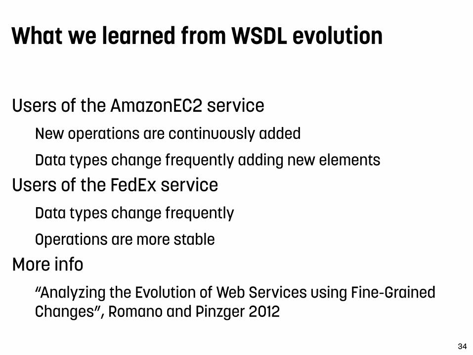
What we learned from WSDL evolution
Users of the AmazonEC2 service New operations are continuously added
Data types change frequently adding new elements Users of the FedEx service
Data types change frequently
Operations are more stable More info
“Analyzing the Evolution of Web Services using Fine-Grained Changes”, Romano and Pinzger 2012
34
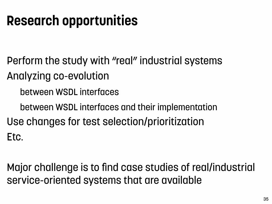
Research opportunities
Perform the study with “real” industrial systems Analyzing co-evolution
between WSDL interfaces
between WSDL interfaces and their implementation Use changes for test selection/prioritization Etc.
Major challenge is to find case studies of real/industrial service-oriented systems that are available
35

FMDiff Evolution of the linux kernel feature model
Nicolas Dintzner, Arie van Deursen, and Martin Pinzger

Linux feature implementation
What is the impact of a feature change?

Main motivation
Identify co-evolution patterns (common changes in the different artifacts implementing a feature)
Local validation of changes to prevent inconsistencies
Facilitate test selection
Prevent variability related implementation bugs Implementation of features is intermixed, leading to undesired interactions Interactions occur between features from different sub-systems demanding cross-subsystem knowledge
More info: “42 variability bugs in the linux kernel: a qualitative analysis”, Abal et al. 2014
38

Extracting feature model changes from the Linux kernel with FMDiff - Nicolas Dintzner
A feature in a Kconfig file
Name
Type & Prompt
Default
Depends
Select
(help text)
Additional structures
39
if ACPI config ACPI_AC tristate "AC Adapter" default y if ACPI depends X86 select POWER_SUPPLY help This driver supports the AC Adapter object ,(...).
endif
Extracting feature model changes from the Linux kernel with FMDiff - Nicolas Dintzner
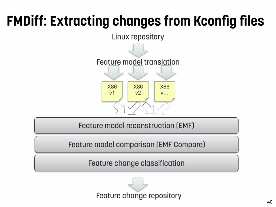
FMDiff: Extracting changes from Kconfig files
40
Linux repository
Feature model translation
X86 v1
X86 v2
X86 v…
Feature model reconstruction (EMF)
Feature model comparison (EMF Compare)
Feature change classification
Feature change repository

Extracting feature model changes from the Linux kernel with FMDiff - Nicolas Dintzner
Feature model transl.: from Kconfig to Kdump
41
if ACPI config ACPI_AC tristate "AC Adapter" default y if ACPI depends X86 select POWER_SUPPLY endif
config ACPI_AC tristate "AC Adapter" default y if ACPI depends X86 && ACPI select POWER_SUPPLY
1- Kconfig (original) 2- Hierarchy flattening
config ACPI_AC tristate "AC Adapter" default y if X86 && ACPI depends X86 && ACPI select POWER_SUPPLY if X86 && ACPI
3- Depends propagation
Item ACPI_AC tristate Prompt ACPI_AC 1 Default ACPI_AC "y" "X86 && ACPI"Depends ACPI_AC "X86 && ACPI" ItemSelects ACPI_AC POWER_SUPPLY "X86 && ACPI”
4- Kdump format (what we use)
Credits to for Undertaker and the translation process

Extracting feature model changes from the Linux kernel with FMDiff - Nicolas Dintzner
FMDiff meta model
42
Feature
Type (string)Prompt (boolean)Depends (string)
DependsReferences (list of strings)
Select Statement
Target (string)Condition (string)
SelectConditionReferences (list of strings)
Default Statement
DefaultValue (string)Condition (string)
DefaultValueReferences (list of strings)DefaultValueConditionReferences (list of strings)
"contains"
"contains"
"contains"
FeatureModel
Architecture (string)Revision (string)
0*
0 *
0 *
Extracting feature model changes from the Linux kernel with FMDiff - Nicolas Dintzner
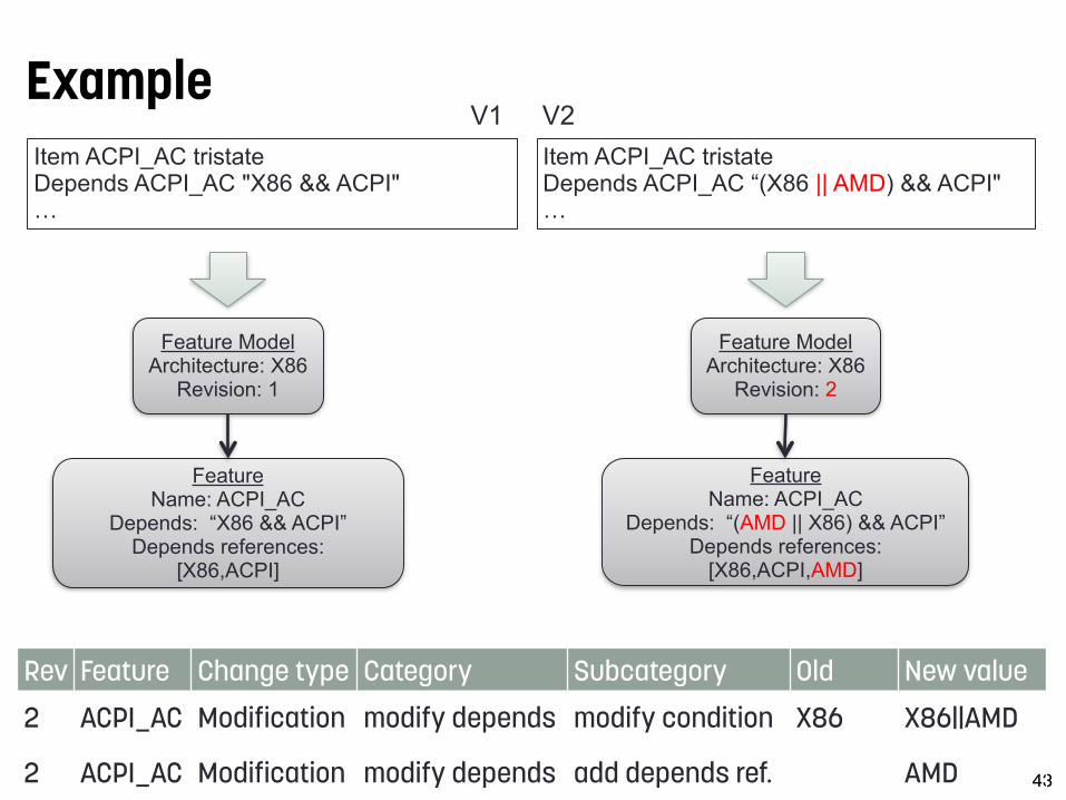
Example
43
Item ACPI_AC tristate Depends ACPI_AC "X86 && ACPI" …
Item ACPI_AC tristate Depends ACPI_AC “(X86 || AMD) && ACPI" …
V1 V2
Feature Model Architecture: X86
Revision: 1
Feature Name: ACPI_AC
Depends: “X86 && ACPI” Depends references:
[X86,ACPI]
Feature Model Architecture: X86
Revision: 2
Feature Name: ACPI_AC
Depends: “(AMD || X86) && ACPI” Depends references:
[X86,ACPI,AMD]
Rev.
Feature Change type Category Subcategory Old value
New value
2 ACPI_AC Modification modify depends modify condition X86 X86||AMD
2 ACPI_AC Modification modify depends add depends ref. AMD

Extracting feature model changes from the Linux kernel with FMDiff - Nicolas Dintzner
Change classification
44
Change operations: Add, Remove, Modify
Attribute Depends Default SelectTypePrompt
ExpressionReferences
Default ValueConditionReferences
TargetConditionReferences
Feature

Study with 14 releases of the linux kernel
45
Feat
ure
chan
ges
cate
gory
dis
trib
utio
n
0%
25%
50%
75%
100%
Linux kernel releases
v2.6.39 v3.0 v3.1 v3.2 v3.3 v3.4 v3.5 v3.6 v3.7 v3.8
ADDEDREMOVEDMODIFIED
493 772 397 1740 612 493 750 609 1068 544

Impact on architectures
Which architectures are affected and need to be tested?
46
Release #changed features % aff. all architectures2.6.39 1016 26.473.0 1020 58.433.2 2361 39.003.4 778 32.393.6 823 34.143.8 963 29.38

What we learned from feature evolution
Modification of existing features is done frequently Should be considered when studying the linux kernel (existing studies mainly focussed on addition and removal of features)
Changes affecting All architectures vary between 10-50% Future studies should be clear about which architectures they study
More info “Analysing the Linux kernel feature model changes using FMDiff”, Dintzner et al. 2015
47
Research opportunities
Link changes in the three implementation spaces Kconfig, Kbuild, source code
Mine co-evolution patterns
Detail the level of changes E.g., consider changes in the conditional statements
Study evolution of other systems E.g., toybox, ecos, BusyBox
Consider frameworks and other highly-configurable systems48

Conclusions
49
ChangeDistiller WSDLDiff
FMDiffif ACPI config ACPI_AC tristate "AC Adapter" default y if ACPI depends X86 select POWER_SUPPLY help This driver supports the AC Adapter object endif
Enrich changes to comprehend them
Martin Pinzger [email protected]