analyzing peer behavior in kad - gnunet report - analyzing peer... · analyzing peer behavior in...
TRANSCRIPT
Institut EurecomDepartment of Corporate Communications
2229, route des CretesB.P. 193
06904 Sophia-AntipolisFRANCE
Research Report RR-07-205Analyzing Peer Behavior in KAD
October 16th, 2007Version 0.02
Moritz Steiner, Taoufik En-Najjary, and Ernst W. Biersack
Tel : (+33) 4 93 00 81 00Fax : (+33) 4 93 00 82 00
Email : {steiner,ennajjar,erbi}@eurecom.fr
1Institut Eurecom’s research is partially supported by its industrial members: BMW Group Re-search & Technology - BMW Group Company, Bouygues Telecom, Cisco Systems, France Telecom,Hitachi, SFR, Sharp, ST Microelectronics, Swisscom, Thales.
1

Institut Eurecom, Sophia–Antipolis, France
AbstractDistributed hash tables (DHTs) have been actively studied in literature
and many different proposals have been made on how to organize peers in aDHT. However, very few DHTs have been implemented in real systems anddeployed on a large scale. One exception is KAD, a DHT based on Kademlia,which is part of eDonkey2000, a peer-to-peer file sharing system with severalmillion simultaneous users. We have been crawling KAD continuously forabout six months and obtained information about geographical distributionof peers, session times, peer availability, and peer lifetime. We also evaluatedto what extent information about past peer uptime can be used to predict theremaining uptime of the peer.
Peers are identified by the so called KAD ID, which was up to now as-sumed to remain the same across sessions. However, we observed that thisis not the case: There is a large number of peers, in particular in China, thatchange their KAD ID, sometimes as frequently as after each session. Thischange of KAD IDs makes it difficult to characterize end-user availabilityor membership turnover. By tracking end-users with static IP addresses, wecould measure the rate of change of KAD ID per end-user.
1 Introduction
Peer-to-peer systems have seen a tremendous growth in the last few years and peer-to-peer traffic makes a major fraction of the total traffic seen in the Internet. Thedominating application for peer-to-peer is file sharing. Some of the most popularpeer-to-peer systems for file sharing have been Napster, FastTrack, BitTorrent, andeDonkey, each one counting a million or more users at their peak time. Since thesesystems are mainly used by home-users and since the content shared is typicallycopyright-protected, the users of these systems often stay only connected as longas it takes for them to download the content they are interested in. As a result, theuser population of these peer-to-peer systems is highly dynamic with peers joiningand leaving all the time.
In this paper, we focus on a single peer-to-peer system, namely KAD, whichis the publishing and search network of eDonkey. We want to characterize KAD
in terms of metrics such as arrival/departure process of peers, session and inter-session lengths, availability, and lifetime.
To obtain the relevant raw data needed we decided to “crawl” KAD. Each crawlgives a snapshot of the peers active at that instant. The three major challenges incrawling are
• Time necessary to carry out a single crawl, which should be as small aspossible to get a consistent view of the system.
• Frequency of the crawls, i.e. the time elapsed between two consecutive crawlsshould be small (no more than a few minutes) in order to achieve a high res-olution for metrics such as session length.
2

• Duration of the crawl, which should be in the order of many months, to beable to correctly capture the longest session and inter-session lengths.
To meet all these goals, we built our own crawler that will be described insection 4.
While peer-to-peer systems have been explored previously using a crawler, theduration of these crawls was limited to a few days at best. We were able to crawlKAD for almost six months at a frequency of one crawl every five minutes, whichallowed us to obtain a number of original results. We observed that:
• session lengths have a “long tail”, with sessions lasting as long as 78 days.
• the distribution of the session lengths is best characterized by a Weibull dis-tribution,with shape parameter k < 1. One property of Weibull distributedsession lengths is that a peer that has so far been up for t units of time will –in expectation – remain up for a duration that is in the order of O(t1−k). Wecan exploit this fact to use the past uptime in order to predict the remaininguptime.
• for many peers, the amount of time a peer is connected per day, called dailyavailability, varies a lot from one day to the next. This makes it difficult topredict daily availability
• the lifetime of a significant fraction of the peers observed can be as shortas a single session. We could explain in part this surprising behavior by thefact that peers change their KAD ID, which is contrary to the assumption thatKAD IDs are persistent.
• when classifying peers according to their geographic origin, the peers fromChina make about 25% of all peers seen at any point of time and Europeis the continent where KAD is most popular. We also saw a big differencebetween peers in China and Europe with respect to some of the key metricssuch as session length or daily availability.
These results provide valuable impact to improve the design and performance ofthe KAD system.
The remainder of the paper is organized as follows. Section 2 presents relatedwork followed by a section describing KAD. Section 4 presents the measurementmethodology followed by two sections that contain the results. In the last Section7 we present our conclusion and an outlook on future work.
2 Related Work
Overnet was the first widely deployed peer-to-peer application that used a DHT,namely Kademlia. The implementation of Overnet is proprietary and its operationwas discontinued in September 2006 after legal actions from the media industry.
3

Overnet has been the subject of several studies such as [2, 7, 13] and up to 265,000concurrent users have been seen online. The study most relevant to our work is theone by Bhagwan et al. [2]. A set of 2,400 peers was contacted every 20 minutesduring two weeks. This study pointed out the IP aliasing problem that is dueto the fact that many peers periodically change their IP address. So, in order toproperly compute session times and other peer-specific metrics one needs to usethe global identifier of the peer-to-peer system. This study also indicates, that forsystems where peers leave permanently, the mean peer availability decreases as theobservation period considered increases.
KAD is the first widely deployed open-source peer-to-peer system relying on aDHT. Two studies on KAD have been published by Stutzbach. The first explainsthe implementation of Kademlia in eMule [19] and the other [20] compares thebehavior of peers in three different peer-to-peer systems, one being KAD. Theresults obtained for KAD are based on crawling a subset of the KAD ID space. Wecall a continuous subset of the total KAD ID space that contains all KAD peerswhose KAD IDs agree in the high order k bits a k-bit zone. [20] crawled a 10-bitzone in 3-4 minutes and a 12-bit zone in approximately 1 minute. A total of 4different zones were crawled during 2 days each. The short duration of the crawlsimplies the maximum values for some metrics such as session up-times or inter-session times that can be observed are naturally limited to 2 days. The paper byStutzbach [20] is the most relevant with respect to our work and we refer to theresults reported by Stutzbach at several occasions. As we will see, some of ourconclusions do not agree with the ones made by Stutzbach, which is in part due tothe fact that a crawl duration of two days is too short to correctly sample KAD withrespect to some of the key metrics such as session durations.
3 Background on KAD
KAD is a Kademlia-based [9] peer-to-peer DHT routing protocol implemented byseveral peer-to-peer applications such as Overnet [14], eMule [5], and aMule [1].The two open–source projects eMule and aMule do have the largest number of si-multaneously connected users since these clients connect to the eDonkey network,which is a very popular peer-to-peer system for file sharing. Recent versions ofthese clients implement the KAD protocol.
Similar to other DHTs like Chord [18], Can [16], or Pastry [17], each KAD nodehas a global identifier, referred to as KAD ID, which is 128 bit long and is randomlygenerated using a cryptographic hash function. The KAD ID is generated when theclient application is started for the first time and is then permanently stored. TheKAD ID stays unchanged on subsequent join and leaves of the peer, until the userdeletes the application or its preferences file1. Therefore, using the KAD ID, aparticular peer can be tracked even after a change of its IP address.
1As we will see later, not all peers in KAD behave this way.
4
3.1 Routing
Routing in KAD is based on prefix matching: Node a forwards a query, destined toa node b, to the node in his routing table that has the smallest XOR-distance. TheXOR-distance d(a, b) between nodes a and b is d(a, b) = a ⊕ b. It is calculatedbitwise on the KAD IDs of the two nodes, e.g. the distance between a = 1011 andb = 0111 is d(a, b) = 1011 ⊕ 0111 = 1100. The fact that this distance metric issymmetric is an advantage compared to other systems, e.g. Chord, since in KAD ifa is close to b, then b is also close to a.
The entries in the routing tables are called contacts and are organized as anunbalanced routing tree: A peer P stores only a few contacts to peers that are faraway in the overlay and increasingly more contacts to peers as we get closer P .For details of the implementation see [19]. For a given distance P knows not onlyone peer but a bucket of peers called contacts. Each bucket can contain up to tencontacts, in order to cope with peer churn without the need to periodically check ifthe contacts are still online.
For routing, a message is simply forwarded to one of the peers from the bucketwith the longest common prefix to the target. Routing to a specific KAD ID isdone in an iterative way, which means that each peer on the way to the destinationreturns the next hop to the sending node. While iterative routing experiences aslightly higher delay than recursive routing, it offers increased robustness againstmessage loss and it greatly simplifies crawling the KAD network.
3.2 Publishing
A key in a peer-to-peer system is an identifier used to retrieve information. KAD
distinguishes between two different keys:
• A source key that identifies the content of a file and is computed by hashingthe content of a file.
• A keyword key that classifies the content of a file and is computed by hash-ing the tokens of the name of a file.
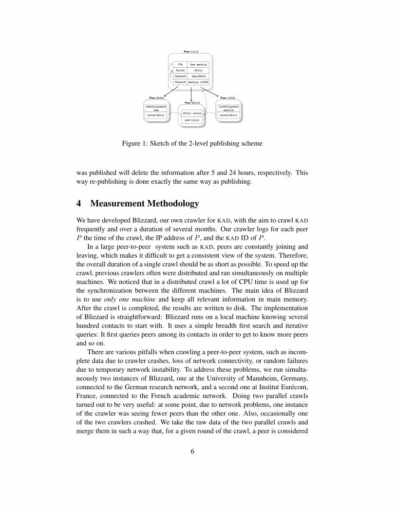
In KAD keys are not published just on a single peer that is numerically closest tothat key, but on 10 different peers whose KAD ID agrees at least in the first 8-bitswith the key. This zone around a key is called the tolerance zone.
Figure 1 shows an example of the publishing process. A peer wants to publish afile with the name the matrix. This filename will result in two keywords, “the”and “matrix”. All relevant references to the real file are generated, such as thesource key and the the keywords with the attached metadata. Next, the keywords“the” and “matrix” are published, pointing to the source. Finally, the source ispublished, pointing to the publishing peer.
Keys are periodically republished: source keys every 5 hours and, keywordkeys every 24 hours. Analogously, a peer on which a source key or keyword key
5
����������
����������
����������
����������
�������������
���
��������������� �����
����������
�������������
����
����������
��������
�����
��� �����
����������
���
�����
�������
�������
Figure 1: Sketch of the 2-level publishing scheme
was published will delete the information after 5 and 24 hours, respectively. Thisway re-publishing is done exactly the same way as publishing.
4 Measurement Methodology
We have developed Blizzard, our own crawler for KAD, with the aim to crawl KAD
frequently and over a duration of several months. Our crawler logs for each peerP the time of the crawl, the IP address of P , and the KAD ID of P .
In a large peer-to-peer system such as KAD, peers are constantly joining andleaving, which makes it difficult to get a consistent view of the system. Therefore,the overall duration of a single crawl should be as short as possible. To speed up thecrawl, previous crawlers often were distributed and ran simultaneously on multiplemachines. We noticed that in a distributed crawl a lot of CPU time is used up forthe synchronization between the different machines. The main idea of Blizzardis to use only one machine and keep all relevant information in main memory.After the crawl is completed, the results are written to disk. The implementationof Blizzard is straightforward: Blizzard runs on a local machine knowing severalhundred contacts to start with. It uses a simple breadth first search and iterativequeries: It first queries peers among its contacts in order to get to know more peersand so on.
There are various pitfalls when crawling a peer-to-peer system, such as incom-plete data due to crawler crashes, loss of network connectivity, or random failuresdue to temporary network instability. To address these problems, we run simulta-neously two instances of Blizzard, one at the University of Mannheim, Germany,connected to the German research network, and a second one at Institut Eurecom,France, connected to the French academic network. Doing two parallel crawlsturned out to be very useful: at some point, due to network problems, one instanceof the crawler was seeing fewer peers than the other one. Also, occasionally oneof the two crawlers crashed. We take the raw data of the two parallel crawls andmerge them in such a way that, for a given round of the crawl, a peer is considered
6
up when he has been seen by at least one crawler.The speed of Blizzard allows us to crawl the entire KAD system (entire KAD ID
space), which was never done before. Such a full crawl of KAD takes about 8 min-utes. The first million different peers are identified in about 10 seconds, the secondmillion in 50 seconds, thereafter the speed of discovery decreases drastically sincemost of the encountered peers have already be seen before during the same crawl.A full crawl of KAD produces about 3 GBytes of inbound and outbound trafficeach.
A full crawl was done three times a day from 2006/08/18 to 2006/08/26 andfrom 2006/10/03 to 2006/10/12. Another full crawl has been started 2007/03/20and is carried out up to now once a day.
A full crawl generates an extremely high amount of trace data and of networktraffic (with peak data rates close to 100 Mbit/sec). Carrying out just 3 crawls perday is not really sufficient to capture the dynamics of KAD at short timescales. Forthis reason, we decided to carry out a zone crawl on a 8-bit zone, where we tryto find all active peers whose KAD ID have the same 8 high-order bits. Such azone crawl, that explores one 256-th of the entire KAD ID space, takes less than2.5 seconds. A zone crawl for the KAD IDs whose 8 high order bits are 0x5b wasdone once every 5 minutes from 2006/09/23 to 2007/03/21, which is slightly lessthan 6 months. We will see in Section 5 that it is possible to infer the results aboutthe entire KAD ID space from the results obtained with a zone crawl.
4.1 Data Cleaning
Crawling happens in “rounds” with a time difference of five minutes, with thetwo crawlers being “synchronized”. A peer that replied to at least one of the twocrawlers during round i is considered to be up at round i .
However, even when crawling from two sites, we realized that it is still possiblethat the requests sent to a peer or its replies can get lost and a peer that is up maybe declared being down. One reason can be that the path between the two crawlersand the peer is disrupted somewhere close to that peer. In this case, the crawlerswill not receive a reply from that peer even when it is up and running. While itis not possible to tell exactly why a peer is not answering, we implemented thefollowing data cleaning rule that we consider “reasonable”: when a peer P that hasbeen reported up at round i − 1 does not reply to either of the two crawlers duringthe next round i, and then replies again during round i+1, then peer P will be alsoconsidered up at round i.
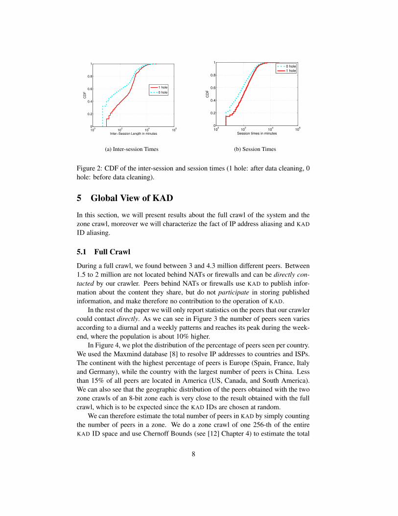
Data cleaning will increase the session and inter-session times. Figure 2(a)plots the cumulative distribution function (CDF) of session and inter-session times.About one third of all inter-session times are just 5 minutes; these values willdisappear after data cleaning, when the smallest inter-session time becomes 10minutes (see 2(a)). Also, after data cleaning some of the adjacent sessions will getmerged and the session times increase (see 2(b)).
7
100
102
104
106
0
0.2
0.4
0.6
0.8
1
CD
F
Inter−Session Length in minutes
1 hole0 hole
(a) Inter-session Times
100
102
104
106
0
0.2
0.4
0.6
0.8
1
Session times in minutes
CD
F
0 hole1 hole
(b) Session Times
Figure 2: CDF of the inter-session and session times (1 hole: after data cleaning, 0hole: before data cleaning).
5 Global View of KAD
In this section, we will present results about the full crawl of the system and thezone crawl, moreover we will characterize the fact of IP address aliasing and KAD
ID aliasing.
5.1 Full Crawl
During a full crawl, we found between 3 and 4.3 million different peers. Between1.5 to 2 million are not located behind NATs or firewalls and can be directly con-tacted by our crawler. Peers behind NATs or firewalls use KAD to publish infor-mation about the content they share, but do not participate in storing publishedinformation, and make therefore no contribution to the operation of KAD.
In the rest of the paper we will only report statistics on the peers that our crawlercould contact directly. As we can see in Figure 3 the number of peers seen variesaccording to a diurnal and a weekly patterns and reaches its peak during the week-end, where the population is about 10% higher.
In Figure 4, we plot the distribution of the percentage of peers seen per country.We used the Maxmind database [8] to resolve IP addresses to countries and ISPs.The continent with the highest percentage of peers is Europe (Spain, France, Italyand Germany), while the country with the largest number of peers is China. Lessthan 15% of all peers are located in America (US, Canada, and South America).We can also see that the geographic distribution of the peers obtained with the twozone crawls of an 8-bit zone each is very close to the result obtained with the fullcrawl, which is to be expected since the KAD IDs are chosen at random.
We can therefore estimate the total number of peers in KAD by simply countingthe number of peers in a zone. We do a zone crawl of one 256-th of the entireKAD ID space and use Chernoff Bounds (see [12] Chapter 4) to estimate the total
8

1.5e+06
2e+06
2.5e+06
3e+06
3.5e+06
4e+06
4.5e+06
Tue Wed Thu Fri Sat Sun Mon Tue Wed Thu
peer
s
date
allresponding
Figure 3: The number of KAD peers available in entire KAD ID space dependingon the time of day.
0
0.05
0.1
0.15
0.2
0.25
GBPTARKRTWUSBRILPLDEITFRESCN
His
togr
am
countries
zone 0x91zone 0xf4full crawl
Figure 4: Histogram of geographic distribution of peers seen on 2006/08/30.
population size and to tightly bound the estimation error.Let N(t)part be the number of peers counted during a zone crawl of an 8–bit
zone at time t and N(t) := 256 ∗ N(t)part the estimate for the total number ofpeers in the KAD system. The true value N(t) for total number of peers at time t isvery close to the estimate N(t), with high probability. More precisely:Prob[|N(t) − N(t)| < 45000] ≥ 0.99, which means that our estimate N(t) hasmost likely an error of less than 3% for a total population of at least 1.5 millionpeers.
Since the full crawl was quite expensive in terms of resources, we will ex-tensively rely on the zone crawl to obtain much of the relevant information aboutKAD.
5.2 Zone Crawl
All the results in the following subsection were obtained using the zone-crawl ofthe 8-bit zone 0x5b that lasted for 179 days.
In Figure 5, we plot the number of peers seen that originate from China andsome European countries. For the peers of each country, we can clearly identify
9
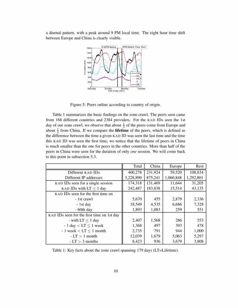
a diurnal pattern, with a peak around 9 PM local time. The eight hour time shiftbetween Europe and China is clearly visible.
Saturday Sunday Monday Tuesday0
200
400
600
800
1000
1200
1400
1600
time of day (CET)
# of
pee
rs a
live
CNESFRITDE
9PM Madrid, Paris, Rom9.30PM Beijing
Figure 5: Peers online according to country of origin.
Table 1 summarizes the basic findings on the zone crawl. The peers seen camefrom 168 different countries and 2384 providers. For the KAD IDs seen the 1stday of our zone crawl, we observe that about 1
3of the peers come from Europe and
about 1
4from China. If we compare the lifetime of the peers, which is defined as
the difference between the time a given KAD ID was seen the last time and the timethis KAD ID was seen the first time, we notice that the lifetime of peers in Chinais much smaller than the one for peers in the other countries. More than half of thepeers in China were seen for the duration of only one session. We will come backto this point in subsection 5.3.
Total China Europe RestDifferent KAD IDs 400,278 231,924 59,520 108,834
Different IP addresses 3,228,890 875,241 1,060,848 1,292,801KAD IDs seen for a single session 174,318 131,469 11,644 31,205
KAD IDs with LT ≤ 1 day 242,487 183,838 15,514 43,135KAD IDs seen for the first time on
- 1st crawl 5,670 455 2,879 2,336- 1st day 18,549 4,535 6,686 7,328
- 60th day 1,893 1,083 259 551KAD IDs seen for the first time on 1st day
- with LT ≤ 1 day 2,407 1,568 286 553- 1 day < LT ≤ 1 week 1,368 497 393 478
- 1 week < LT ≤ 1 month 2,735 791 944 1,000- LT > 1 month 12,039 1,679 5,063 5,297- LT > 3 months 8,423 936 3,679 3,808
Table 1: Key facts about the zone crawl spanning 179 days (LT=Lifetime).
10

Arrivals and Departures
Since we crawl KAD once every 5 minutes, we can determine the number of peersthat join and leave between two consecutive crawls. Knowing the arrival rate ofpeers is useful since it allows to model the load in KAD due to newly joining peers.Each time a peer joins, it first contacts other peers for information to populate itsrouting table, before it publishes the keywords and source keys for all the files itwill share.
In figure 6(a) we depict the CDF (cumulative distribution function) of the num-ber of peers that arrive and that depart between two consecutive crawls. We see thatthe distributions for arrivals and departures are the same. This is to be expected,since we observe the system in “steady state”: in this case, the system should be-have like G/G/∞, for which, according to Little’s Law, the arrival rate is equal tothe departure rate [11].
The arrival process is very well described by a Negative Binomial distribution(see figure 6(b))
0 50 100 150 200 2500
0.2
0.4
0.6
0.8
1
No. of host
CD
F
mean=114.79, std=29.93
ArrivalsDepartures
(a) CDF of the number of arrivals and de-partures.
0 50 100 150 200 2500
0.005
0.01
0.015
Number of Arrivals
PD
F
Negative Binomial Parameters: r=16.81, p=0.127
ArrivalsNegative Binomial
(b) PDF of the number of arrivals
Figure 6: Peer arrivals between two crawls during the first week.
5.3 Aliasing
IP Address Aliasing
It has been known for quite some time [2, 7] that peers may get frequently assignednew IP addresses, which is referred to as IP address aliasing. We observed a totalof 400,278 distinct KAD IDs and 3,228,890 different IP addresses (see table 1).As we see in figure 7, the number of different IP addresses per peer is stronglycorrelated with the peer lifetime.
11

100
101
102
103
104
0
0.2
0.4
0.6
0.8
1
number of different IP addresses
CD
F
LT <= 1 day1 day < LT <= 1 week1 week < LT <= 1 month1 month < LT
Figure 7: The number of different IP addresses reported per KAD ID during aperiod of six months.
KAD ID Aliasing
Figure 8 reports the number of new KAD IDs per day. i.e. KAD IDs seen for the firsttime, according to country of origin. More than 50% of the new KAD IDs are frompeers in China, which is more than one order of magnitude more than the numberof new KAD IDs seen for any other country such as Spain, France, or Germany.
We see in our zone crawl approx. 2,000 new KAD IDs a day, which means thatfor the entire KAD system the number of new KAD IDs per day is around 500,000.If we extrapolate, this makes about 180 Million KAD IDs a year. It is hard tobelieve that there exist such a large number of different end-users of KAD.
20 40 60 80 100 120 140 160 18010
1
102
103
104
Days
Num
ber o
f new
pee
rs
all
chinaspain
France
Germany
Figure 8: New KAD IDs according to country of origin.
We were curious to find out whether the end-users really stop using KAD afterone session, or whether the same users come back with a different KAD ID. We re-fer to the phenomenon of non-persistent KAD IDs as KAD ID aliasing, in contrastto IP address aliasing.
To investigate KAD ID aliasing, we need to look for peers with static IP ad-dresses, wich we can track for non-persistent KAD IDs. We know that, for instancein France, one of the ADSL providers (Proxad) assigns static IP addresses to cus-
12
tomers located in areas where the service offer is completely “un-bundled”, whileFrance Telecom-Orange changes the IP addresses of ADSL customers on a dailybasis.
To find peers with static IP addresses, we started in March 20th, 2007 to carryout one full crawl a day. We take the logs of the two full crawls of March 20thand March 30th and extract the 160,641 peers that have the same IP address andthe same KAD ID in both logs. We call this set of IP addresses pivot set. Ourhypothesis is that a peer that keeps the same IP address for 10 days is assigned astatic IP address. We then take the logs of the full crawls starting April 1st, 2007 tolook for peers whose IP addresses are in the pivot set that have changed their KAD
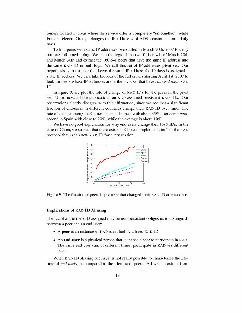
ID.In figure 9, we plot the rate of change of KAD IDs for the peers in the pivot
set. Up to now, all the publications on KAD assumed persistent KAD IDs. Ourobservations clearly disagree with this affirmation, since we see that a significantfraction of end-users in different countries change their KAD ID over time. Therate of change among the Chinese peers is highest with about 35% after one month,second is Spain with close to 20%, while the average is about 10%.
We have no good explanation for why end-users change their KAD IDs. In thecase of China, we suspect that there exists a “Chinese implementation” of the KAD
protocol that uses a new KAD ID for every session.
0 10 20 30 400
0.05
0.1
0.15
0.2
0.25
0.3
0.35
0.4
days after pivot crawl
% o
f pee
rs s
een
that
cha
nged
thei
r KA
D ID
ChinaSpainTotalFranceProxad
Figure 9: The fraction of peers in pivot set that changed their KAD ID at least once.
Implications of KAD ID Aliasing
The fact that the KAD ID assigned may be non-persistent obliges us to distinguishbetween a peer and an end-user:
• A peer is an instance of KAD identified by a fixed KAD ID.
• An end-user is a physical person that launches a peer to participate in KAD.The same end-user can, at different times, participate in KAD via differentpeers.
When KAD ID aliasing occurs, it is not really possible to characterize the life-time of end-users, as compared to the lifetime of peers. All we can extract from
13

our crawl data is the lifetime of peers, which provides us with a lower bound onthe lifetime of end-users.
6 Peer View
In this section, we will present metrics that describe the behavior of individualpeers, such as lifetime, session and inter-session time, residual uptime, and dailyavailability using the observations made with our 179 day zone crawl.
We will mainly focus on the peers that were first seen on the 1st day of ourcrawl, since we could observe them for the longest period of time. For reference,we will occasionally compare the results with those obtained for the peers seen thefirst time on day 60. We have chosen day 60, since the largest inter-session timesobserved very rarely exceed 60 days, which allows us to assume that the peers wesee for the first time on day 60 have newly joined the system.
6.1 Lifetime of Peers
We recall that, among the peers seen on the first day, about 2/3 of the peers havea lifetime larger than one month and close to 45% have a lifetime even larger thanthree months (Table 1).
For a given KAD ID k, let tj1(k) be the time this KAD ID is seen joining KAD
for the first time, and let tlm(k) be the time this KAD ID seen for the last time.The lifetime of KAD ID k is defined as tl
m(k) − tj1(k). Since our crawl is of finite
duration, we can never be sure if a peer with KAD ID k will not come back after westopped crawling. To make such a event very unlikely, we have decided to computethe lifetime only for peers with KAD IDs that have seen that last time 60 days ormore before the end of our crawl (remember that the inter-session times seen arevery rarely larger than 60 days!). Since at time tl
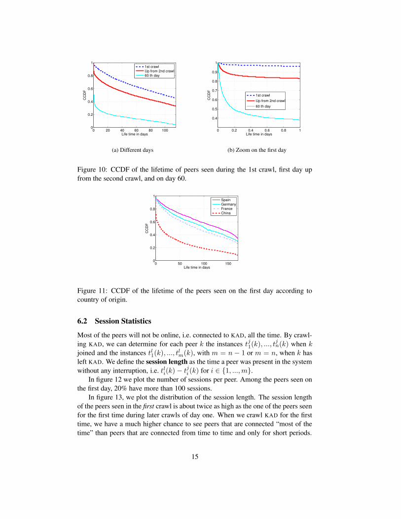
m(k) we do not know whetherpeer k will re-join KAD later, it is clear that our definition of lifetime gives a lowerbound on the actual lifetime of a peer. Figure 10 depicts the the CCDF of lifetimefor KAD IDs seen for the first time during the first crawl, on the first day, and forthe first time on the 60th day. It is striking to notice that the KAD IDs first seen onday 60 have a much lower lifetime than the KAD IDs seen the first day. In fact, only40% of the KAD IDs that were first seen on day 60 will be seen for more than onedays (Figure 10(b)). As we know from table 1, more than half of the KAD IDs firstseen on day 60 are from peers in China; it is for these peers that we could clearlyestablish that participants change their KAD IDs.
Figure 11 depicts the complementary cumulative distribution (CCDF) of thepeers seen the the first day. There is a big difference in the lifetime of peers fromChina as compared to Europe: more than a third of the Chinese peers disappearafter only one day and only 10% have a lifetime of more than 150 days, whileclose to 40% of the peers in Europe have a lifetime of more than 150 days.
14
0 20 40 60 80 1000
0.2
0.4
0.6
0.8
1
Life time in days
CC
DF
1st crawlUp from 2nd crawl60 th day
(a) Different days
0 0.2 0.4 0.6 0.8 1
0.4
0.5
0.6
0.7
0.8
0.9
1
Life time in days
CC
DF
1st crawlUp from 2nd crawl60 th day
(b) Zoom on the first day
Figure 10: CCDF of the lifetime of peers seen during the 1st crawl, first day upfrom the second crawl, and on day 60.
0 50 100 1500
0.2
0.4
0.6
0.8
1
Life time in days
CC
DF
SpainGermanyFranceChina
Figure 11: CCDF of the lifetime of the peers seen on the first day according tocountry of origin.
6.2 Session Statistics
Most of the peers will not be online, i.e. connected to KAD, all the time. By crawl-ing KAD, we can determine for each peer k the instances tj
1(k), ..., tjn(k) when k
joined and the instances tl1(k), ..., tlm(k), with m = n − 1 or m = n, when k hasleft KAD. We define the session length as the time a peer was present in the systemwithout any interruption, i.e. tl
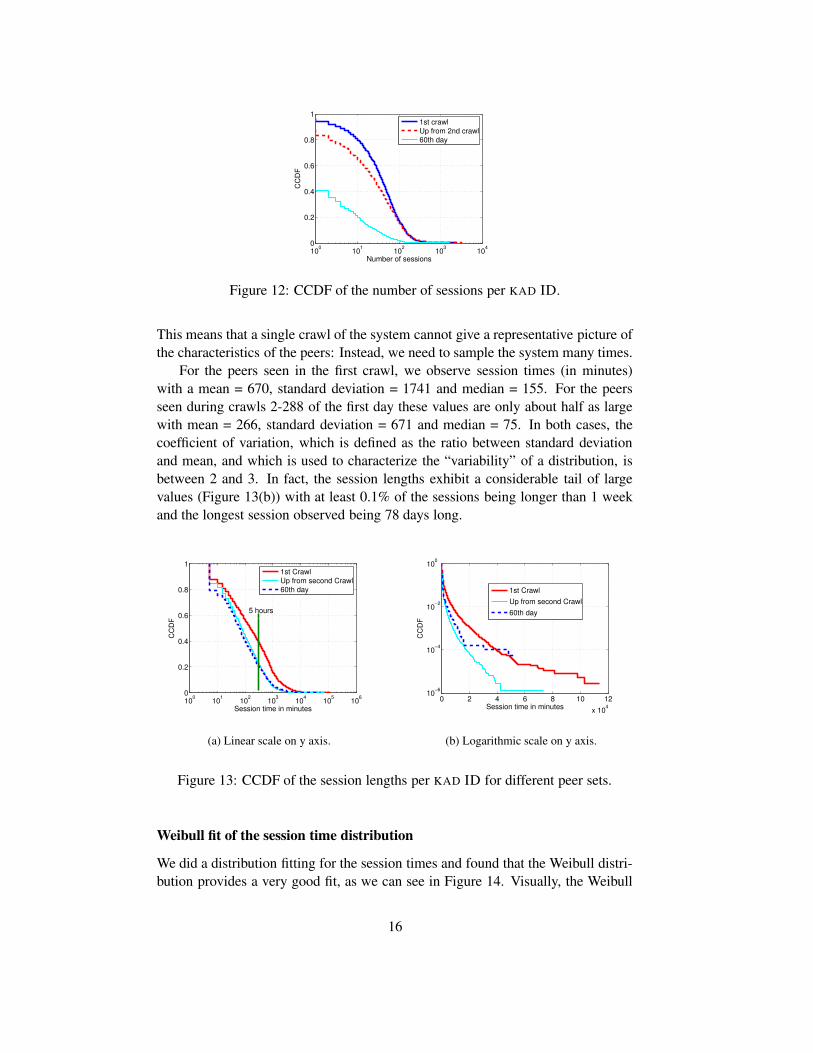
i(k) − tji (k) for i ∈ {1, ...,m}.In figure 12 we plot the number of sessions per peer. Among the peers seen on
the first day, 20% have more than 100 sessions.In figure 13, we plot the distribution of the session length. The session length
of the peers seen in the first crawl is about twice as high as the one of the peers seenfor the first time during later crawls of day one. When we crawl KAD for the firsttime, we have a much higher chance to see peers that are connected “most of thetime” than peers that are connected from time to time and only for short periods.
15
100
101
102
103
104
0
0.2
0.4
0.6
0.8
1
Number of sessions
CC
DF
1st crawlUp from 2nd crawl60th day
Figure 12: CCDF of the number of sessions per KAD ID.
This means that a single crawl of the system cannot give a representative picture ofthe characteristics of the peers: Instead, we need to sample the system many times.
For the peers seen in the first crawl, we observe session times (in minutes)with a mean = 670, standard deviation = 1741 and median = 155. For the peersseen during crawls 2-288 of the first day these values are only about half as largewith mean = 266, standard deviation = 671 and median = 75. In both cases, thecoefficient of variation, which is defined as the ratio between standard deviationand mean, and which is used to characterize the “variability” of a distribution, isbetween 2 and 3. In fact, the session lengths exhibit a considerable tail of largevalues (Figure 13(b)) with at least 0.1% of the sessions being longer than 1 weekand the longest session observed being 78 days long.
100
101
102
103
104
105
106
0
0.2
0.4
0.6
0.8
1
Session time in minutes
CC
DF
1st CrawlUp from second Crawl60th day
5 hours
(a) Linear scale on y axis.
0 2 4 6 8 10 12
x 104
10−6
10−4
10−2
100
Session time in minutes
CC
DF
1st CrawlUp from second Crawl60th day
(b) Logarithmic scale on y axis.
Figure 13: CCDF of the session lengths per KAD ID for different peer sets.
Weibull fit of the session time distribution
We did a distribution fitting for the session times and found that the Weibull distri-bution provides a very good fit, as we can see in Figure 14. Visually, the Weibull
16

distribution adequately tracks the dominant shape of the measured distribution: Us-ing only the session length samples larger than 15 minutes, the fit passes the Kol-mogorov-Smirnov (goodness of fit) test. However, for the small session lengthsof 5, 10, or 15 minutes, the fit is not good due to the too large granularity of timebetween two crawls (5 minutes).
101
102
103
104
105
106
0
0.2
0.4
0.6
0.8
1
Session Time in minutes
CD
F
mean=670.6789,std=1741.3677,scale=357.7152,shape=0.54512
Session TimesWeibull
(a) First crawl
101
102
103
104
105
106
0
0.2
0.4
0.6
0.8
1
Session Time in minutes
CD
F
mean=266.5358,std=671.5063,scale=169.5385,shape=0.61511
Session TimesWeibull
(b) Up from 2nd crawl
Figure 14: Weibull fit of the session time distribution of the peers seen first day.
The Weibull distribution has two parameters k > 0 (shape) and λ > 0 (scale).For k < 1 the Weibull distribution is part of the class of the so called subexpo-nential distributions, for which the tail decreases more slowly than any exponentialtail [6]. This implies that knowing the past (uptime) of a peer allows to predict thefuture (residual uptime). More formally, if S denotes the session length then theexpected residual uptime E[S − t|S > t] ∼ O(t1−k), i.e. it grows sub-linearly ascompared to the Pareto distribution, where the growth is linear, i.e. O(t).
Stutzbach [20] observed that the Weibull distribution provides a good fit forthe session lengths of the BitTorrent traces. However, due to significant undercounting of long sessions in the KAD traces, Stutzbach was not able to determinewhich distribution best describes the session length of the KAD trace.
Figure 15 shows the expected residual uptime for the scale and shape valuesthat describe the session length of peers seen in the first crawl. There is a nice fitbetween the empirical values and the interpolation using a function whose growthis O(t1−k). We see that for small observed uptime values the remaining expecteduptime values are considerable: A peer that has been up for 500 minutes will havea remaining expected uptime of 1,000 minutes.
One occasion where it would be interesting to exploit the knowledge that ses-sion lengths are Weibull distributed is in dynamically adjusting the expiration timesof the source keys published: We saw that in section 3.2 that a source key that pointsto the peer will expire 5 hours after it has been published. On the other hand, weobserved that the median session length of peers is 155 minutes or less. Also, fig-ure 13(a) indicates that less than 40% of the peers have a session length of 5 hoursor more. This means that in more than 60% of the cases the peer that publishes asource key will leave KAD before the pointer to the file it owns will expire. As a
17

result, many of the pointers to sources in KAD will be stale. A more appropriatepolicy might be to first publish a source key with an expiration time much smallerthan 5 hours and progressively increase the expiration time as the uptime of thepeer that owns the file increases.
0
500
1000
1500
2000
2500
0 1000 2000 3000 4000E
xpec
ted
Res
idua
l Upt
ime
(min
)Observed uptime (min)
Numerical integrationinterpolation with O(x1-k)
Figure 15: Expected residual uptime for k = 0.54, λ = 357.
Next Session Time
One may ask the question whether consecutive sessions are correlated in length. Ifthere is a strong positive correlation, one could use information about past sessionlengths as predictor for the length of future sessions. Such a prediction could, forinstance, be used by a publishing peer to choose the optimal value for the timeduring which information it publishes in KAD should be valid.
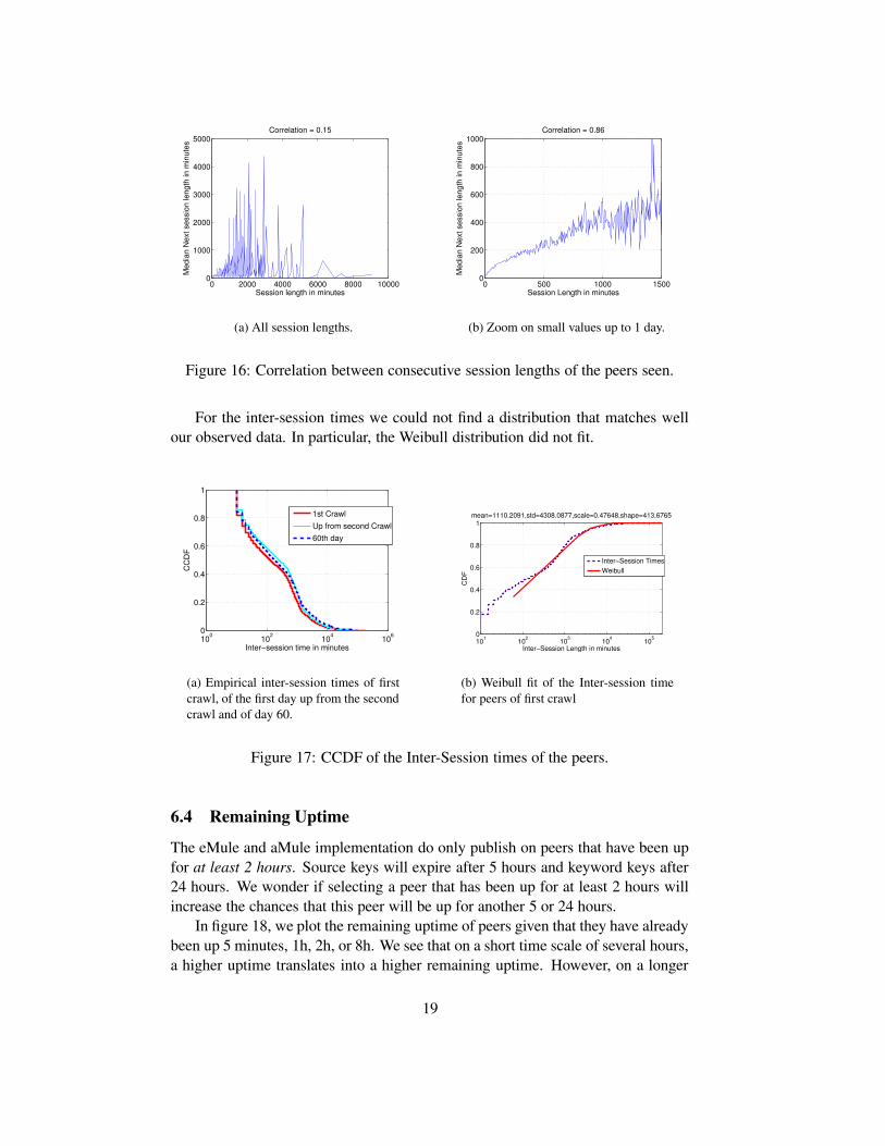
If we take all session length samples and compute the coefficient of correlationover consecutive session length we get a value of 0.15, which indicates that thereis almost no correlation. For a visual depiction see figure 16(a). However, if oneonly considers session lengths up to 1 day, there is considerable positive correla-tion (correlation = 0.85) as can be also seen from figure 16(b). Stutzbach ([20]figure 10(b)), who could only observe session lengths up to one day found a strongcorrelation. This example nicely illustrates how incomplete data due to too shortcrawling duration can have a major impact on the conclusion one is able to drawfrom the observations.
6.3 Inter-Session Time
The inter-session time is defined as the time a peer k is continuously absent fromthe system, i.e. tji+1
(k) − tli(k) for i ∈ {1, ..., n}. Figure 17 depicts the CCDFof the inter-session times. As it was already the case for the session times, thedistribution of the inter-session times of the peers seen during the first crawl issmaller than the one of the peers seen during later crawls. The same is true forthe mean inter-session time (1110.2 min. vs. 1349.8 min.). The peers first seen onday 60, which mainly come from China, have even larger inter-session times and amean inter-session time of 1704.3.
18
0 2000 4000 6000 8000 100000
1000
2000
3000
4000
5000
Session length in minutes
Med
ian
Nex
t ses
sion
leng
th in
min
utes
Correlation = 0.15
(a) All session lengths.
0 500 1000 15000
200
400
600
800
1000
Session Length in minutes
Med
ian
Nex
t ses
sion
leng
th in
min
utes
Correlation = 0.86
(b) Zoom on small values up to 1 day.
Figure 16: Correlation between consecutive session lengths of the peers seen.
For the inter-session times we could not find a distribution that matches wellour observed data. In particular, the Weibull distribution did not fit.
100
102
104
106
0
0.2
0.4
0.6
0.8
1
Inter−session time in minutes
CC
DF
1st CrawlUp from second Crawl60th day
(a) Empirical inter-session times of firstcrawl, of the first day up from the secondcrawl and of day 60.
101
102
103
104
105
0
0.2
0.4
0.6
0.8
1
Inter−Session Length in minutes
CD
F
mean=1110.2091,std=4308.0877,scale=0.47648,shape=413.6765
Inter−Session TimesWeibull
(b) Weibull fit of the Inter-session timefor peers of first crawl
Figure 17: CCDF of the Inter-Session times of the peers.
6.4 Remaining Uptime
The eMule and aMule implementation do only publish on peers that have been upfor at least 2 hours. Source keys will expire after 5 hours and keyword keys after24 hours. We wonder if selecting a peer that has been up for at least 2 hours willincrease the chances that this peer will be up for another 5 or 24 hours.
In figure 18, we plot the remaining uptime of peers given that they have alreadybeen up 5 minutes, 1h, 2h, or 8h. We see that on a short time scale of several hours,a higher uptime translates into a higher remaining uptime. However, on a longer
19

timescale of one day or more, the past uptime will not make much of a difference.This behavior was predicted by the expected residual uptime (Figure 15).
This means that minimum age-based peer selection as implemented in eMuleand aMule is quite effective when publishing source keys that will expire after 5hours, but not for keyword keys that will expire after one day. Also, only about20% of the peers with an uptime of 2 hours will remain up for at least another 24hours. Therefore, the only way to ensure that keywords remain available for 24hours is to publish information about a keyword on more than one peer, as it isdone by eMule and aMule.
101
102
103
104
105
106
0
0.1
0.2
0.3
0.4
0.5
0.6
0.7
0.8
0.9
1
Uptime Remaining in minutes
CC
DF
Up 8hUp 2hUp 1h5 min
One Day5 hours
Figure 18: CCDF of the remaining uptime of peers, given the uptime so far, forpeers seen in first crawl.
6.5 Availability
Characterizing availability is important for building efficient distributed applica-tions such as overlay multicast or distributed file systems. For instance, availability-guided file placement can help reduce the cost of object maintenance [10], whichcan be potentially prohibitive, as it was pointed out by Blake [3]. The availabilityduring the interval [T, T + ∆] of a KAD ID that was first seen at time T is definedas the sum of the times the KAD ID was seen during the interval [T, T + ∆] di-vided by the length of the interval ∆. This definition implies that a KAD ID k thathas not been seen beyond time tlm(k) will see its availability strictly decreasingfor increasing values of ∆ that satisfy tl
m(k) < T + ∆. For this reason,it we willlater introduce a second notion of availability that considers only the period duringwhich the KAD ID was observed.
Figure 19 depicts the CDF of the mean peer availability computed for differentintervals ∆. As it has already been seen by Bhagwan [2], in a peer-to-peer systemwith churn, the mean availability decreases as the period over which availability iscomputed increases, which is due to the fact that some peers may have permanentlyleft KAD. For large values of ∆, the availability keeps decreasing. However, forshort values for ∆ such as 1, 2, or 5 days, there is a significant fraction of peers(30%, 15%, 5%) that have an availability of one.
20

0 0.2 0.4 0.6 0.8 10
0.1
0.2
0.3
0.4
0.5
0.6
0.7
0.8
0.9
1
availability
CD
F
140 days100 days30 days15 days5 days2 days1 day
Figure 19: CCDF The availability of peers seen on the first day.
Given that the availability of a peer over the last N days is known, we want tostudy how accurate the future availability of a peer can be predicted knowing itspast behavior.
To do so we take the peers with an average availability larger than 0.8 duringthe first N days and ask how well the availability values from the past predict thefuture availability. In figure 25(a) we see that a high availability of 0.8 in the past30 days will result in more the 60% of the cases in an at least as high availabilityfor the next 30 days. As we increase the prediction horizon to N = 140 daysthe distribution of the future availability becomes almost uniform, which meansthat in a real system (with permanent departure), the long term availability at dayN = 140 can not be predicted knowing the availability of the past 30 days. The setof peers considered in figure 25(a) contains peers that leave the system definitivelybefore N days, i.e. their lifetime < N days. However, as we have seen before, thereis considerable KAD ID aliasing (see section 5.3), which implies that the actualend-user lifetime will in many cases be larger than measured the KAD ID lifetime.To get an “upper bound” on how well we could predict end-user availability in thebest case, when there are no permanent departures, we consider in figure 25(b)only the peers whose lifetime is at least 100 days. In this case, a high availabilityof 0.8 in the past 30 days will result in more than 75% of the cases in an at least ashigh availability for the next 30 days and in 60% of the case even for the next 50days (N = 80).
6.6 Daily Availability
Daily availability measures the fraction of time a peer is connected per day. Dailyavailability expresses the “intensity” of participation of users in the exchange offiles. For a given peer P , we define daily availability of P as the percentage oftime P was seen on that day. For a peer that was first seen on day i and last seenon day j, we will get a time series of daily availability values that has j − i + 1elements.
Peers in China spend much less time per day connected than peers in Europe
21

0 0.2 0.4 0.6 0.8 10
0.2
0.4
0.6
0.8
1
availability
CC
DF
Proba( availability after N days | availability after 30 days>0.8)
N=40 daysN=50 daysN=60 daysN=80 daysN=100 daysN=140 days
(a) All peers seen first day.
0 0.2 0.4 0.6 0.8 10
0.2
0.4
0.6
0.8
1
availability
CC
DF
P(availability after N days | availability after 30 days >=0.8
N=40 daysN=50 daysN=60 daysN=80 daysN=100 days
(b) Peers seen first day with a lifetime ≥
100 days.
Figure 20: Conditional distribution of the availability over N days, given the avail-ability over the first 30 days larger than 0.8.
(Figure 21). The “online times” for peers in Europe are quite impressive, with 40%of the peers being connected more than 5 hours per day and 20% even more than10 hours per day.
0 5 10 15 20 250
0.2
0.4
0.6
0.8
1
Mean daily−availability in hours
CD
F
First day, liftime<= 2 months
China
Europe
Figure 21: CDF of the mean daily availability of peers seen the first day.
Next day availability
Daily availability measures how many hours a peer is connected per day. Observ-ing this metric over several days or weeks can give an indication about the stabilityof peer participation in KAD over time. Stutzbach ([20], figure (11b)) compared thedaily availability of peers between the 2 days of his crawl. For all peers with a givenavailability value on day one, he computed the median availability of these peerson day 2 of the crawl. A plot of the availability on the first days vs. median avail-ability on the second day indicated that both values as positively correlated. We did
22
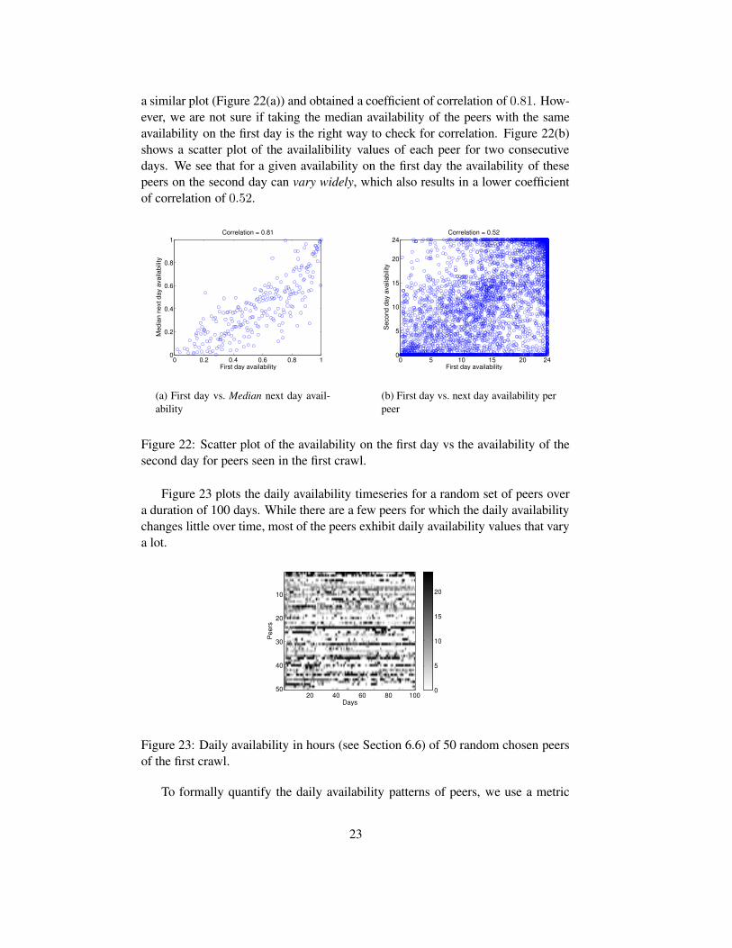
a similar plot (Figure 22(a)) and obtained a coefficient of correlation of 0.81. How-ever, we are not sure if taking the median availability of the peers with the sameavailability on the first day is the right way to check for correlation. Figure 22(b)shows a scatter plot of the availalibility values of each peer for two consecutivedays. We see that for a given availability on the first day the availability of thesepeers on the second day can vary widely, which also results in a lower coefficientof correlation of 0.52.
0 0.2 0.4 0.6 0.8 10
0.2
0.4
0.6
0.8
1
First day availability
Med
ian
next
day
ava
ilabi
lity
Correlation = 0.81
(a) First day vs. Median next day avail-ability
0 5 10 15 20 240
5
10
15
20
24
First day availability
Sec
ond
day
avai
labi
lity
Correlation = 0.52
(b) First day vs. next day availability perpeer
Figure 22: Scatter plot of the availability on the first day vs the availability of thesecond day for peers seen in the first crawl.
Figure 23 plots the daily availability timeseries for a random set of peers overa duration of 100 days. While there are a few peers for which the daily availabilitychanges little over time, most of the peers exhibit daily availability values that varya lot.
Days
Pee
rs
20 40 60 80 100
10
20
30
40
50 0
5
10
15
20
Figure 23: Daily availability in hours (see Section 6.6) of 50 random chosen peersof the first crawl.
To formally quantify the daily availability patterns of peers, we use a metric
23

called approximate entropy (ApEn), which is a “regularity statistic” that quan-tifies the unpredictability of fluctuations in a time series. For details on the approx-imate entropy see [15]. This metric was recently used by Mickens [10] to analyzeseveral traces of machine availabilities such as the Microsoft trace and the Overnettrace. We calculate ApEn of the daily availability of KAD peers seen on the firstday. The smaller the value for ApEn, the more regular the daily availability patternover time. However, if the time series is highly irregular, the occurrence of similaravailability patterns will be very unlikely for the following days, and ApEn willbe relatively large.
We could confirm the results of Mickens for the Microsoft trace (see figure24(a)), where 80% of the values of ApEn(2) are close to zero, which indicates thatdaily availability varies little over time. On the other hand, the ApEn(2) values forthe KAD trace a much higher (see figure 24(b)). About 50% of the peers the peershave ApEn(2) values above 0.5, which indicates that the daily availability valuesare quite irregular. Mickens made a similar observation for the Overnet trace.
0 0.1 0.2 0.3 0.4 0.50
0.2
0.4
0.6
0.8
1
Approximate entropy
CD
F
Microsoft traces, m=2
(a) Microsoft trace, m=2
−0.2 0 0.2 0.4 0.6 0.8 1 1.20
0.2
0.4
0.6
0.8
1
Approximate Entropy
CD
F
First crawl, life time>30, m=2
Spain
ChinaFrance
Germany
(b) Peers seen in the first day
Figure 24: CDF of the approximate entropy.
We also checked if the daily availability behavior of the peers exhibits any di-urnal pattern. Douceur[4] analyzed different traces of machine availability2 fromMicrosoft, Internet, Gnutella, and Napster. Using Fourier transformation he foundcyclic behavior in the daily availability of the Microsoft machines, but did not findany diurnal patterns for the other traces. We did a Fourrier and Wavelet transfor-mation on the daily availability timeseries of our KAD peers and could not find anycyclic behavior or diurnal patterns.
2The trace is available athttp://www.cs.berkeley.edu/˜pbg/availability/
24
6.7 Availability Prediction
Given that the availably of a peer over the last N days is known, we want to studyhow accurate the future availability of a peer can be predicted knowing it’s pastbehavior. In all the experiments we consider the peers that were seen the first dayof the crawl or a subset of these peers.
We start with a very simple experiment, where we only take the peers with anaverage availability larger than 0.8 during the first N days and ask how well theavailability values from the past predict the future availability.
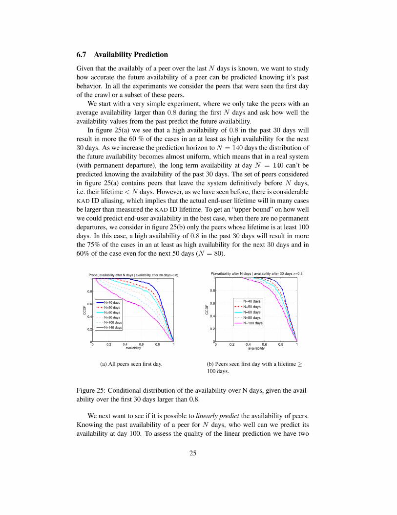
In figure 25(a) we see that a high availability of 0.8 in the past 30 days willresult in more the 60 % of the cases in an at least as high availability for the next30 days. As we increase the prediction horizon to N = 140 days the distribution ofthe future availability becomes almost uniform, which means that in a real system(with permanent departure), the long term availability at day N = 140 can’t bepredicted knowing the availability of the past 30 days. The set of peers consideredin figure 25(a) contains peers that leave the system definitively before N days,i.e. their lifetime < N days. However, as we have seen before, there is considerableKAD ID aliasing, which implies that the actual end-user lifetime will in many casesbe larger than measured the KAD ID lifetime. To get an “upper bound” on how wellwe could predict end-user availability in the best case, when there are no permanentdepartures, we consider in figure 25(b) only the peers whose lifetime is at least 100days. In this case, a high availability of 0.8 in the past 30 days will result in morethe 75% of the cases in an at least as high availability for the next 30 days and in60% of the case even for the next 50 days (N = 80).
0 0.2 0.4 0.6 0.8 10
0.2
0.4
0.6
0.8
1
availability
CC
DF
Proba( availability after N days | availability after 30 days>0.8)
N=40 daysN=50 daysN=60 daysN=80 daysN=100 daysN=140 days
(a) All peers seen first day.
0 0.2 0.4 0.6 0.8 10
0.2
0.4
0.6
0.8
1
availability
CC
DF
P(availability after N days | availability after 30 days >=0.8
N=40 daysN=50 daysN=60 daysN=80 daysN=100 days
(b) Peers seen first day with a lifetime ≥
100 days.
Figure 25: Conditional distribution of the availability over N days, given the avail-ability over the first 30 days larger than 0.8.
We next want to see if it is possible to linearly predict the availability of peers.Knowing the past availability of a peer for N days, who well can we predict itsavailability at day 100. To assess the quality of the linear prediction we have two
25

measures:
• The correlation coefficient indicates the strength and direction of a linearrelationship between two random variables. The correlation is 1 in the caseof an increasing linear relationship, -1 in the case of a decreasing linear rela-tionship, and some value in between in all other cases, indicating the degreeof linear dependence between the variables. The closer the coefficient is toeither -1 or 1, the stronger the correlation between the variables. However,correlation alone is be sufficient to evaluate this relationship between twovariables.
• The coefficient of determination, R2, measures the goodness of the globalfit of the model. Specifically, R2 takes a value in [0,1] that represents theproportion of variability in Yi that may be attributed to some linear combina-tion of the regressors (explanatory variables) in X. To consider the predictionto be good if R2 ≥ 0.9 Thus, R2 = 1 indicates that the fitted model explainsall variability in y, while R2 = 0 indicates no linear relationship betweenthe response variable and regressors.
As before we use all the peers seen the first day to get a “lower bound” onhow well linear prediction works (see figure 26(a)) and all the peers seen the firstday whose lifetime is greater than 100 days to get an “upper bound” (see figure26(b)). To have a good prediction of the availability, we need to know at least theavailability over the first 70 days, if we take all peers, and over the first 50 days, ifwe take only the peers that stay for at least 100 days.
0 20 40 60 80 1000
0.2
0.4
0.6
0.8
1
Days
linear prediction of 100th day availability
DeterminationCorrelation
(a) All peers seen in the first Crawl (5669peers)
0 20 40 60 80 1000
0.2
0.4
0.6
0.8
1
Days
Linear prediction of 100th day availability
DetrminationCorrelation
(b) Peers seen in the first crawl withlifetime≥ 100 days (2823 peers)
Figure 26: Linear predictability of the availability over 100 days given the avail-ability over the first N days.
26

7 Conclusion and Future Work
We have presented results on the peer behavior in KAD, the largest currently de-ployed DHT. The duration of our crawl was 179 days, which makes it to our knowl-edge, the longest crawl of a peer-to-peer system ever carried out.
The speed of our crawler allowed us to crawl the entire KAD systems and theresults we obtained could be used to validate our approach to crawl in the followingmostly a single zone whose results will be representative for the entire system.
The most important findings are that session lengths are Weibull distributed,and that session length and daily availability varies a lot for a given peer. Also, KAD
IDs are not necessarily persistent as was assumed so far. Nevertheless, the mostimportant metrics such as session times, inter-session times or daily availability arenot affected by the non-persistent KAD IDs.
It remains an open problem to explain why KAD IDs are non-persistent andunder what circumstances peers change their KAD ID. To be able to model thelifetime of peers we need to find a method that allows to characterize the processof permanent departure for end-users as opposed to peers.
This paper contributes to a better quantitative understanding of the peer dy-namics in KAD. However, the current implementation of KAD in eMule and eMuledoes not yet exploit this knowledge. Instead, some important parameters such asthe expiration time of keys or the number of copies are static. While we havealready commented on some of the parameter choices in the paper. We feel thatour work opens numereous interesting perspectives for improving the design andimplementation of KAD.
AcknowledgmentWe would like to thank D. Carra and F. Pianese for feedback on an early versionof this paper. We also thank the Computing Center of the University of Mannheimfor providing us with the resources necessary to carry out such a long crawl.
27
References[1] A-Mule. http://www.amule.org/.
[2] R. Bhagwan, S. Savage, and G. Voelker. Understanding availability. In Proceedingsof the 2nd International Workshop on Peer-to-Peer Systems (IPTPS’03), pages 256–267, 2003.
[3] C. Blake and R. Rodrigues. High availability, scalable storage, dynamic peer net-works: Pick two. In HotOs 03, 03.
[4] J. Douceur. Is remote host availabilty governed by a universal law. In SigmetricsPerformance Evaluation Review, 2003.
[5] E-Mule. http://www.emule-project.net/.
[6] C. Goldie and C. Klueppelberg. Subexponential distributions. In R. Adler, R. Feld-man, and M. Taqqu, editors, A Practical Guide to Heavy Tails: Statistical Techniquesfor Analysing Heavy Tails. Birkhauser, Basel, 1997.
[7] K. Kutzner and T. Fuhrmann. Measuring large overlay networks - the overnet exam-ple. In Proceedings of the 14th KiVS, Feb. 2005.
[8] Maxmind. http://www.maxmind.com/.
[9] P. Maymounkov and D. Mazieres. Kademlia: A Peer-to-peer informatiion systembased on the XOR metric. In Proceedings of the 1st International Workshop on Peer-to-Peer Systems (IPTPS), pages 53–65, Mar. 2002.
[10] J. Mickens and B. Noble. Exploiting availability prediction in distributed systems. InProc. 2006 NSDI, 2006.
[11] I. Mitrani. Probabilistic Modelling. Cambridge University Press, 1998.
[12] M. Mitzenmacher and E. Upfal. Probability and Computing: Randomized Algorithmsand Probabilistic Analysis. Cambridge Press, 2005.
[13] N. Naoumov and K. Ross. Exploiting p2p systems for ddos attacks. In InternationalWorkshop on Peer-to-Peer Information Management, May 2006.
[14] Overnet. http://www.overnet.org/.
[15] S. M. Pincus. Approximate entropy as a mesure of system complexity. In Proceedingsof the National Academy of Science, 88:2297–2301, December 1990.
[16] S. Ratnasamy, M. Handley, R. Karp, and S. Shenker. A scalable content-addressablenetwork. In Proc. ACM SIGCOMM, 2001.
[17] A. Rowstron and P. Druschel. Pastry: Scalable, distributed object location and rout-ing for large-scale Peer-to-peer systems. In Proceedings of Middleware, Heidelberg,Germany, November 2001.
[18] I. Stoica, R. Morris, D. Karger, M. Kaashoek, and H. Balakrishnan. Chord: A scal-able Peer-to-peer lookup service for Internet applications. In Proceedings of SIG-COMM, pages 149–160, San Diego, CA, USA, 2001. ACM Press.
[19] D. Stutzbach and R. Rejaie. Improving lookup performance over a widely-deployedDHT. In Proc. Infocom 06, Apr. 2006.
[20] D. Stutzbach and R. Rejaie. Understanding churn in peer-to-peer networks. In Proc.Internet Measurement Conference (IMC), Oct. 2006.
28