Analyzing Real Estate, Financial Sector, and Sovereign Risks and Economic Impact Using Contingent Claims

Analysis: Framework and Application to Ireland

May 25, 2014

Dale F. Gray1

Monetary and Capital Markets Department International Monetary Fund

Abstract

This paper presents a conceptual framework with some applications to analyze credit risk and feedbacks between banks, sovereigns, households, other sectors as well as economic output for an economy based on contingent claims analysis (CCA). Risk transmission from between banks and sovereigns can arise from explicit and implicit government guarantees and other channels. In order to understand banking risk exposures and associated public sector contingent liabilities in times of stress, CCA is applied to construct risk-adjusted (economic) balance sheets of financial institutions and sovereigns that are interconnected via implicit put options embedded in risky debt and guarantees. The structural CCA model, with its embedded fundamental volatility, helps explain complex risk transmission and feedbacks. The conceptual framework is expanded to economy-wide interlinked CCA balance sheets and applied to Ireland during 2002- 2011 to analyze nonlinear risk transfer to banks from real estate prices and household mortgage debt, and from banks to the sovereign as well as economic output. The interlinked economy-wide risk framework is able to capture non-linear risk transmission between sectors and impacts on economic output in ways that cannot be measured or analyzed with traditional flow macroeconomic accounts. Presented at the Macro Financial Modeling Group Meeting, May 30-31, 2014

1 Email: Dgray@imf.org

2

Table of Contents Page

I. Introduction……………………………………………………………………..3

II. Risk-adjusted Balance Sheets using Contingent Claims Analysis……………...3

Risk-Adjusted Balance (CCA) Sheets for Banks and Financial Institutions…...4

Risk-Adjusted Balance (CCA) Sheets for Sovereigns………………………….5

Economy-wide Inter-linked CCA Balance Sheets……………………………..7

III. Example Application to Ireland During the Recent Crisis……………………..9 Bank Risks and Market Implied Guarantees………………………………….12 Credit Growth Trend, GDP Growth and Market Value of Assets……………14 Sovereign Balance Sheet Estimates…………………………………………..15 Household Balance Sheets……………………………………………………17 Commercial Real Estate and Corporate Sector Risk…………………………19 Expected Losses Transmitted to Banks, Market Implied Guarantee and Actual Losses………………………………………………………………………...20 Relating CCA Balance Sheet Indicators to Consumption and Investment…..22 Further Work and Applications………………………………………………23 Appendix 1 - Contingent Claims Analysis…………………………………...24 Appendix 2 - How the Inter-linked CCA Economy Model is Related to the Traditional Macroeconomic Accounts……………………………………….26 References……………………………………………………………………31

The author would like to thank Robert C. Merton, Andy Lo, Sam Malone, Andy Jobst, Jianping Zhou, Dimitri Demekas, Marco Gross, Matthias Sydow, Joan Paredes and Conn Creeden for helpful comments and discussion of these ideas

3

I. Introduction

This paper is consists of two parts. Section II describes contingent claims analysis (CCA) and how it can be used to calibrate risk-adjusted balance sheets of corporate and financial firms and measure credit risk. The application of CCA to sovereigns is described and the framework to analyze bank-sovereign risk transmission and feedbacks is discussed. The framework is expanded to an economy-wide framework of inter-linked CCA models including the corporate, household, and commercial real estate sectors. Section III is an application of the model to Ireland 2002-2011 at various points in time beginning with real estate boom, then bust, severe banking sector crisis and transmission of risk to the sovereign via guarantees and the subsequent sovereign crisis.

II. Risk-adjusted Balance Sheets using Contingent Claims Analysis

Contingent Claims Analysis (CCA) represents a generalization of the option pricing theory pioneered by Black and Scholes (1973) and Merton (1973), and, thus, is forward-looking by construction, providing a consistent framework based on current market conditions rather than on purely historical experience. When applied to the analysis and measurement of credit risk, it is commonly called the Merton Model. CCA is a risk-adjusted balance sheet of firms, based on three principles: (i) the values of liabilities (equity and debt) are derived from assets; (ii) liabilities have different priorities (i.e. senior versus junior claims); and, (iii) assets follow a stochastic process. The value of promised payments on debt constitutes a default barrier. When assets fall below the default barrier, this triggers a default event.

When there is a chance of default, the repayment of debt is considered “risky,” to the extent that repayment of the full face value of debt is not guaranteed in the event of default. Risky debt is composed of two parts: the default-free value of debt and deposits, minus the “expected loss to creditors” from default over a specific time horizon. The expected loss component, as demonstrated by Merton (1974), can be expressed as the value of an implicit put option on the value of the borrower assets, whose strike price is equal to the default barrier (default-free debt value).

The risk-adjusted balance sheet uses market values, whereas the accounting balance sheet uses accounting values. The risk-adjusted balance sheet includes the value of the implicit put and call options, which are respectively equal to the expected loss component of the risky (defaultable) debt and the risky market value of equity.

There are several different calibration methods that can be applied to infer values for parameters in CCA-style models, ranging from simple two variable procedures such as the one described in Merton (1974), to variations and commercial applications such as MKMV (2003) now called Moody’s CreditEdge. Other techniques can include the use of bond/CDS prices or other asset prices.

4

The market value of assets of corporations and financial institutions cannot be

observed directly but can be implied using financial asset prices. From the observed prices and volatilities of market-traded securities, one can estimate the implied asset values and volatilities of the underlying assets in financial institutions. In the traditional Merton (1974) model, for example, the calibration procedure requires knowledge about value of equity, E, the volatility of equity, EV , and the distress barrier, B, as inputs into equations

0 1 2( ) ( ) rTE A N d B e N d and 1

( )V V E A

E A N d in order to calculate the two unknowns, the implied asset value A and implied asset volatility,V

A. Once the asset value and asset

volatility have been estimated, expected losses to firm (or bank) creditors can be calculated. Asset value and asset volatility, together with the default barrier, time horizon, and the risk-free discount rate r, are used to calculate the values of the implicit put option, EP , which is the expected loss to creditors (see Appendix 1 for more details. Merton (1977) shows how the value of government guarantees to banks and valuation of deposit insurance can be calculated using implicit put options in the CCA framework for banks.2 An economy-wide model of interlinked CCA balance sheets can be constructed to analyze risk transmission (see Gray et al. 2008 and Gray and Malone 2008). The accounting balance sheet can be “derived” from the special case of the risk-adjusted balance sheet—the case where there is uncertainty is set to zero (i.e. assets have no volatility). With zero volatility on the balance sheets, the expected loss to bank creditors goes to zero and equity becomes book equity. The credit risk exposure cannot be measured.

Risk-Adjusted Balance (CCA) Sheets for Banks and Financial Institutions

In order to understand risk exposures (and associated public sector contingent liabilities) in times of stress, CCA is applied to construct risk-adjusted (economic) balance sheets of financial institutions. The total market value of firm assets, A, at any time, t, is equal to the sum of its equity market value, E, and its risky debt, D. The asset value follows a random, continuous process and may fall below the value of outstanding liabilities, which constitute the bankruptcy level (‘default threshold’ or ‘distress barrier’) B.3 B is defined as the present value of promised payments on debt and deposits discounted at the risk free rate. The value of risky debt is equal to default-free debt minus the present value of expected loss due to default.

In this framework, expected losses associated with outstanding liabilities can be valued as an implicit put option and its cost reflected in a credit spread above the risk-free 2 Also see Merton (1992, 1998, and 2002), Gray, Merton, and Bodie (2002, 2007, and 2008).

3 Moody’s KMV CreditEdge defines this barrier equal to total short-term debt plus one-half of long-term debt.

5

rate that compensates investors for holding risky debt. In this paper we will use an advanced CCA model for banks which uses accounting balance sheet, equity market information, and CDS/bond spread information. The advanced CCA can be used to infer the implicit or explicit government guarantees/contingent liabilities. If we define

EPD as the fraction of expected losses (

EP is the implicit put option derived from equity market and debt information using CCA) covered by the government this is a measure of value of the government’s guarantee or its contingent liability. The risk retained by the financial institution and reflected in the CDS spreads for that institution is thus 1 EPD . The difference between credit spread implied by the CCA (called a fair-value CDS spread) and the actual observed CDS spread can be used to infer the size of government guarantee/contingent liabilities. This is because the observed CDS spread is depressed due to the impact of implicit or explicit government guarantees. (See Gapen 2009, Merton et al. 2013, Gray et al. 2013.)

Risk-Adjusted Balance (CCA) Sheets for Sovereigns

The CCA approach can be adapted to the sovereign, but the procedure for doing so generally depends on whether one is dealing with an emerging market sovereign with significant foreign debt, usually denominated in hard currency, or a developed country sovereign, in which most or all debt is issued in local currency. The adaptation of CCA models for the analysis of sovereign credit risk is a relatively recent phenomenon, and is based on work by Gray et al. (2007 and 2008), Gapen et al. (2008), Gray and Malone (2008), Gray and Jobst (2010a). The application of the sovereign CCA model in this paper focuses on developed country sovereigns, especially European sovereigns, such as Ireland or Spain. The value of sovereign assets at time horizon T, relative to the promised payments on sovereign debt (the sovereign debt or distress barrier) is the driver of these expected losses. The value of sovereign debt can be seen as having two components, the default-free value (promised payment value) and the expected loss associated with default in the event the assets are insufficient to meet the promised payments.

The application of the sovereign CCA model to developed country sovereigns requires us to infer the value of sovereign assets—because the value of sovereign assets is not directly observable—based upon measures of expected losses on sovereign debt derived from the full term structure of sovereign CDS spreads. See Box 1 for details (further information is in Gray and Jobst 2011, and Gray and Malone 2012).

6

Box 1. Calibrating the Sovereign CCA Balance Sheet and the Link to Financial Sector

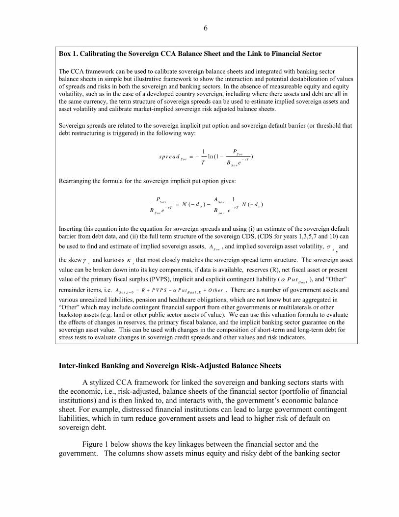
The CCA framework can be used to calibrate sovereign balance sheets and integrated with banking sector balance sheets in simple but illustrative framework to show the interaction and potential destabilization of values of spreads and risks in both the sovereign and banking sectors. In the absence of measureable equity and equity volatility, such as in the case of a developed country sovereign, including where there assets and debt are all in the same currency, the term structure of sovereign spreads can be used to estimate implied sovereign assets and asset volatility and calibrate market-implied sovereign risk adjusted balance sheets.

Sovereign spreads are related to the sovereign implicit put option and sovereign default barrier (or threshold that debt restructuring is triggered) in the following way:

1ln (1 )S o v

S o v rTS o v

Psp re a d

T B e

Rearranging the formula for the sovereign implicit put option gives:

2 1(1

( ) )S o v S o vrT rT

S o v so v

N dP A

N dB e B e

Inserting this equation into the equation for sovereign spreads and using (i) an estimate of the sovereign default barrier from debt data, and (ii) the full term structure of the sovereign CDS, (CDS for years 1,3,5,7 and 10) can be used to find and estimate of implied sovereign assets, S o vA , and implied sovereign asset volatility,

AV , and

the skewA

J and kurtosis A

N that most closely matches the sovereign spread term structure. The sovereign asset value can be broken down into its key components, if data is available, reserves (R), net fiscal asset or present value of the primary fiscal surplus (PVPS), implicit and explicit contingent liability (D B a n kP u t ), and “Other”

remainder items, i.e. , 0 ,S o v t B a n k EA R P V P S P u t O th e rD . There are a number of government assets and various unrealized liabilities, pension and healthcare obligations, which are not know but are aggregated in “Other” which may include contingent financial support from other governments or multilaterals or other backstop assets (e.g. land or other public sector assets of value). We can use this valuation formula to evaluate the effects of changes in reserves, the primary fiscal balance, and the implicit banking sector guarantee on the sovereign asset value. This can be used with changes in the composition of short-term and long-term debt for stress tests to evaluate changes in sovereign credit spreads and other values and risk indicators.

Inter-linked Banking and Sovereign Risk-Adjusted Balance Sheets

A stylized CCA framework for linked the sovereign and banking sectors starts with the economic, i.e., risk-adjusted, balance sheets of the financial sector (portfolio of financial institutions) and is then linked to, and interacts with, the government’s economic balance sheet. For example, distressed financial institutions can lead to large government contingent liabilities, which in turn reduce government assets and lead to higher risk of default on sovereign debt.

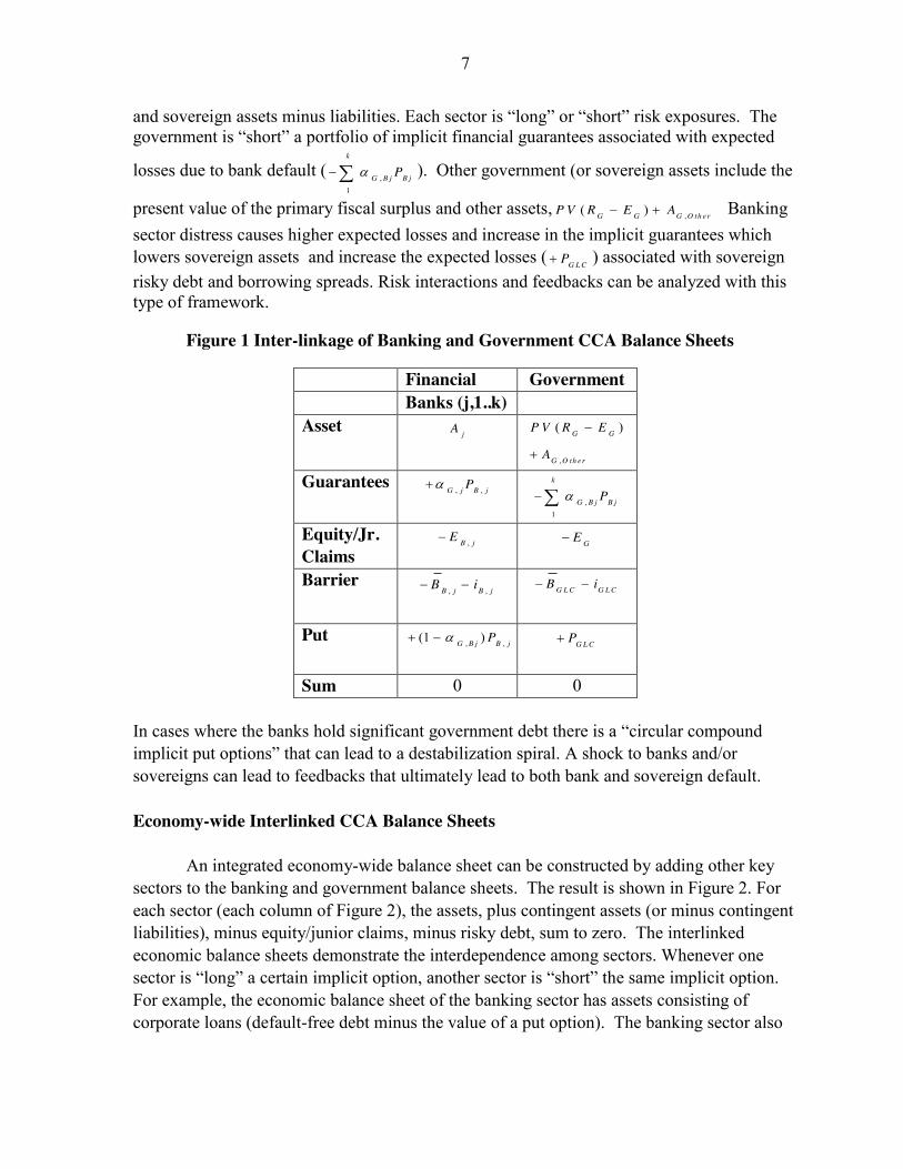
Figure 1 below shows the key linkages between the financial sector and the government. The columns show assets minus equity and risky debt of the banking sector

7

and sovereign assets minus liabilities. Each sector is “long” or “short” risk exposures. The government is “short” a portfolio of implicit financial guarantees associated with expected

losses due to bank default ( ,1

k

G B j B jPD¦ ). Other government (or sovereign assets include the

present value of the primary fiscal surplus and other assets, ,( )G G G O th e rP V R E A Banking sector distress causes higher expected losses and increase in the implicit guarantees which lowers sovereign assets and increase the expected losses ( G L CP ) associated with sovereign risky debt and borrowing spreads. Risk interactions and feedbacks can be analyzed with this type of framework.

Figure 1 Inter-linkage of Banking and Government CCA Balance Sheets

Financial Government Banks (j,1..k) Asset

jA

,

( )G G

G O th e r

P V R E

A

Guarantees , ,G j B jPD

,1

k

G B j B jPD¦

Equity/Jr. Claims

,B jE GE

Barrier , ,B j B jB i

G L C G L CB i

Put , ,(1 )G B j B jPD

G L CP

Sum 0 0 In cases where the banks hold significant government debt there is a “circular compound implicit put options” that can lead to a destabilization spiral. A shock to banks and/or sovereigns can lead to feedbacks that ultimately lead to both bank and sovereign default. Economy-wide Interlinked CCA Balance Sheets

An integrated economy-wide balance sheet can be constructed by adding other key sectors to the banking and government balance sheets. The result is shown in Figure 2. For each sector (each column of Figure 2), the assets, plus contingent assets (or minus contingent liabilities), minus equity/junior claims, minus risky debt, sum to zero. The interlinked economic balance sheets demonstrate the interdependence among sectors. Whenever one sector is “long” a certain implicit option, another sector is “short” the same implicit option. For example, the economic balance sheet of the banking sector has assets consisting of corporate loans (default-free debt minus the value of a put option). The banking sector also

8

includes contingent liabilities (implicit put options) from the government as an asset, which is an obligation (short put option) on the government’s economic balance sheet. Banks’ assets contain risky debt of the corporate sector, commercial real estate risky loans and risky household mortgage debt. Corporate sector assets are a function of investment (I).

Figure 2 Economy-wide Contingent Claim Balance Sheet with Risk Exposures Across Sectors (Implicit Put and Call Options)

Corp Commercial Households Financial Government Foreign Real Estate H BS H RE Banks (j,1..k) Asset ( ( ))C PA f I

C R EA

,

F IN

L

H R E

A

A

E

,H R EA jA

,

( )G G

G O th e r

P V R E

A

Cont. A & L

, ,G j B jPD

,1

k

G B j B jPD¦

Equity/Jr. Claims

CE C R EE H

H

E

C

,H R EE

,B jE

GE Foreign Claims

Barrier C

C

B

i

C R E

C R E

B

i

,

,

H R E

H R E

B

i

, ,B j B jB i

G L C G L CB i

Put CP C R EP

,H R EP

, ,(1 )G B j B jPD

G L CP

Sum 0 0 0 0 0 0 0 Source: Adapted from Gray and Malone 2008 and Gray, Merton, Bodie 2008

For the household sector, asset HA is the sum of the household sector’s financial wealth F INA , the present value of its labor income LA , and equity ,H R EE in real estate. The debt of households to banks and non-banks is frequently tied to homes and real estate. For this reason it is practical to have two segregated but linked household CCA balance sheets. The “subsidiary” balance sheet would have real estate assets as the primary asset and related debt would be on the liability side.4 The households “equity” in real estate is modeled as call option on real estate assets .H R EA minus risky household mortgage related debt , ,H R E H R EB P .

4 There are many variations of this structure. Debt could be including on the main household balance sheet or additional subsidiary balance sheets could be included relating specific debt obligations to related assets. The legal insolvency framework for mortgages varies by country, so in some cases this simple model would need to be modified.

9

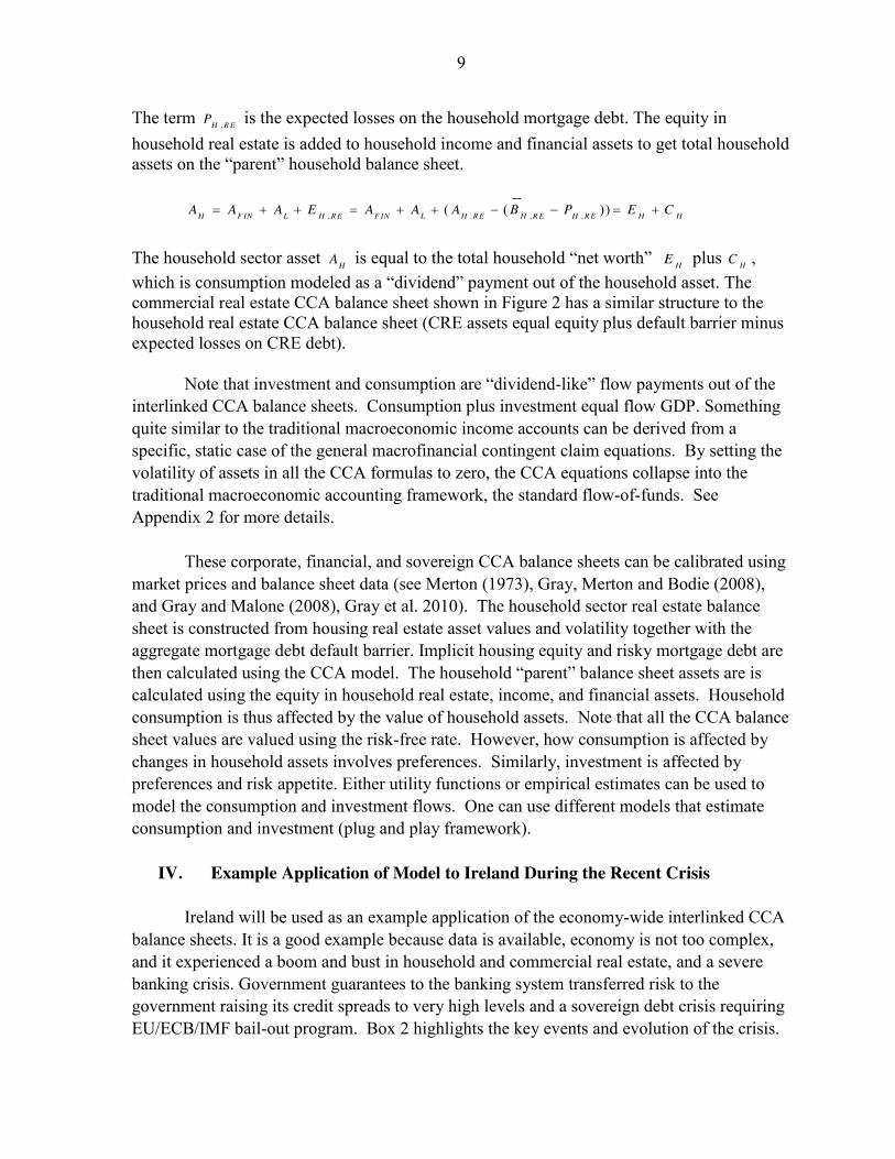
The term ,H R EP is the expected losses on the household mortgage debt. The equity in household real estate is added to household income and financial assets to get total household assets on the “parent” household balance sheet.

, . , ,( ( ))H F IN L H R E F IN L H R E H R E H R E H HA A A E A A A B P E C

The household sector asset HA is equal to the total household “net worth” HE plus HC , which is consumption modeled as a “dividend” payment out of the household asset. The commercial real estate CCA balance sheet shown in Figure 2 has a similar structure to the household real estate CCA balance sheet (CRE assets equal equity plus default barrier minus expected losses on CRE debt).

Note that investment and consumption are “dividend-like” flow payments out of the interlinked CCA balance sheets. Consumption plus investment equal flow GDP. Something quite similar to the traditional macroeconomic income accounts can be derived from a specific, static case of the general macrofinancial contingent claim equations. By setting the volatility of assets in all the CCA formulas to zero, the CCA equations collapse into the traditional macroeconomic accounting framework, the standard flow-of-funds. See Appendix 2 for more details.

These corporate, financial, and sovereign CCA balance sheets can be calibrated using

market prices and balance sheet data (see Merton (1973), Gray, Merton and Bodie (2008), and Gray and Malone (2008), Gray et al. 2010). The household sector real estate balance sheet is constructed from housing real estate asset values and volatility together with the aggregate mortgage debt default barrier. Implicit housing equity and risky mortgage debt are then calculated using the CCA model. The household “parent” balance sheet assets are is calculated using the equity in household real estate, income, and financial assets. Household consumption is thus affected by the value of household assets. Note that all the CCA balance sheet values are valued using the risk-free rate. However, how consumption is affected by changes in household assets involves preferences. Similarly, investment is affected by preferences and risk appetite. Either utility functions or empirical estimates can be used to model the consumption and investment flows. One can use different models that estimate consumption and investment (plug and play framework).

IV. Example Application of Model to Ireland During the Recent Crisis

Ireland will be used as an example application of the economy-wide interlinked CCA balance sheets. It is a good example because data is available, economy is not too complex, and it experienced a boom and bust in household and commercial real estate, and a severe banking crisis. Government guarantees to the banking system transferred risk to the government raising its credit spreads to very high levels and a sovereign debt crisis requiring EU/ECB/IMF bail-out program. Box 2 highlights the key events and evolution of the crisis.

10

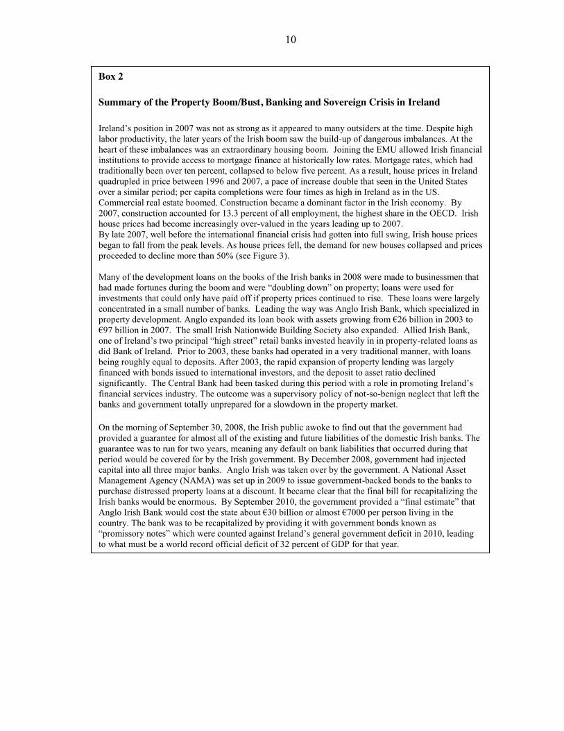
Box 2 Summary of the Property Boom/Bust, Banking and Sovereign Crisis in Ireland Ireland’s position in 2007 was not as strong as it appeared to many outsiders at the time. Despite high labor productivity, the later years of the Irish boom saw the build-up of dangerous imbalances. At the heart of these imbalances was an extraordinary housing boom. Joining the EMU allowed Irish financial institutions to provide access to mortgage finance at historically low rates. Mortgage rates, which had traditionally been over ten percent, collapsed to below five percent. As a result, house prices in Ireland quadrupled in price between 1996 and 2007, a pace of increase double that seen in the United States over a similar period; per capita completions were four times as high in Ireland as in the US. Commercial real estate boomed. Construction became a dominant factor in the Irish economy. By 2007, construction accounted for 13.3 percent of all employment, the highest share in the OECD. Irish house prices had become increasingly over-valued in the years leading up to 2007. By late 2007, well before the international financial crisis had gotten into full swing, Irish house prices began to fall from the peak levels. As house prices fell, the demand for new houses collapsed and prices proceeded to decline more than 50% (see Figure 3). Many of the development loans on the books of the Irish banks in 2008 were made to businessmen that had made fortunes during the boom and were “doubling down” on property;; loans were used for investments that could only have paid off if property prices continued to rise. These loans were largely concentrated in a small number of banks. Leading the way was Anglo Irish Bank, which specialized in property development. Anglo expanded its loan book with assets growing from €26 billion in 2003 to €97 billion in 2007. The small Irish Nationwide Building Society also expanded. Allied Irish Bank, one of Ireland’s two principal “high street” retail banks invested heavily in in property-related loans as did Bank of Ireland. Prior to 2003, these banks had operated in a very traditional manner, with loans being roughly equal to deposits. After 2003, the rapid expansion of property lending was largely financed with bonds issued to international investors, and the deposit to asset ratio declined significantly. The Central Bank had been tasked during this period with a role in promoting Ireland’s financial services industry. The outcome was a supervisory policy of not-so-benign neglect that left the banks and government totally unprepared for a slowdown in the property market. On the morning of September 30, 2008, the Irish public awoke to find out that the government had provided a guarantee for almost all of the existing and future liabilities of the domestic Irish banks. The guarantee was to run for two years, meaning any default on bank liabilities that occurred during that period would be covered for by the Irish government. By December 2008, government had injected capital into all three major banks. Anglo Irish was taken over by the government. A National Asset Management Agency (NAMA) was set up in 2009 to issue government-backed bonds to the banks to purchase distressed property loans at a discount. It became clear that the final bill for recapitalizing the Irish banks would be enormous. By September 2010, the government provided a “final estimate” that Anglo Irish Bank would cost the state about €30 billion or almost €7000 per person living in the country. The bank was to be recapitalized by providing it with government bonds known as “promissory notes” which were counted against Ireland’s general government deficit in 2010, leading to what must be a world record official deficit of 32 percent of GDP for that year.

11

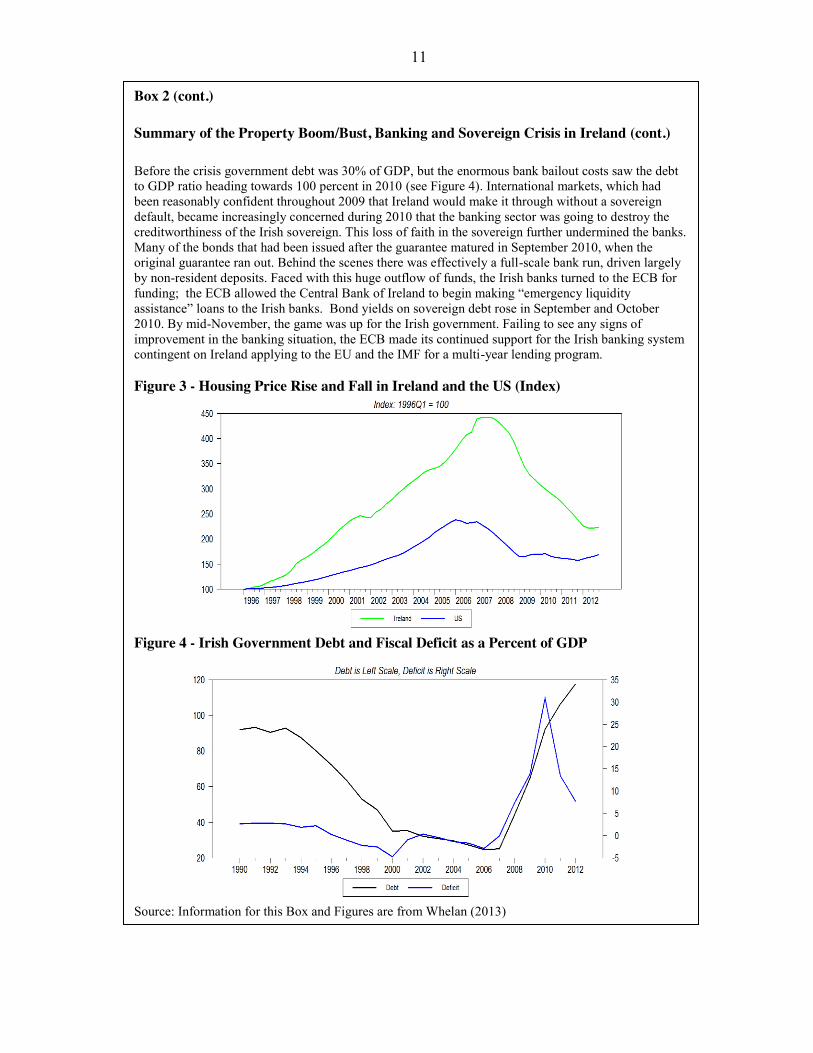
Box 2 (cont.) Summary of the Property Boom/Bust, Banking and Sovereign Crisis in Ireland (cont.) Before the crisis government debt was 30% of GDP, but the enormous bank bailout costs saw the debt to GDP ratio heading towards 100 percent in 2010 (see Figure 4). International markets, which had been reasonably confident throughout 2009 that Ireland would make it through without a sovereign default, became increasingly concerned during 2010 that the banking sector was going to destroy the creditworthiness of the Irish sovereign. This loss of faith in the sovereign further undermined the banks. Many of the bonds that had been issued after the guarantee matured in September 2010, when the original guarantee ran out. Behind the scenes there was effectively a full-scale bank run, driven largely by non-resident deposits. Faced with this huge outflow of funds, the Irish banks turned to the ECB for funding;; the ECB allowed the Central Bank of Ireland to begin making “emergency liquidity assistance” loans to the Irish banks. Bond yields on sovereign debt rose in September and October 2010. By mid-November, the game was up for the Irish government. Failing to see any signs of improvement in the banking situation, the ECB made its continued support for the Irish banking system contingent on Ireland applying to the EU and the IMF for a multi-year lending program. Figure 3 - Housing Price Rise and Fall in Ireland and the US (Index)

Figure 4 - Irish Government Debt and Fiscal Deficit as a Percent of GDP

Source: Information for this Box and Figures are from Whelan (2013)

12

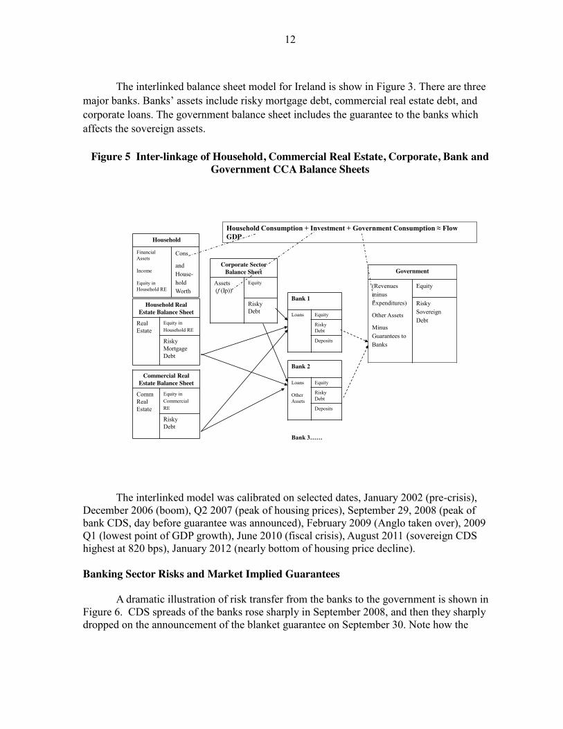
The interlinked balance sheet model for Ireland is show in Figure 3. There are three major banks. Banks’ assets include risky mortgage debt, commercial real estate debt, and corporate loans. The government balance sheet includes the guarantee to the banks which affects the sovereign assets.

Figure 5 Inter-linkage of Household, Commercial Real Estate, Corporate, Bank and Government CCA Balance Sheets

The interlinked model was calibrated on selected dates, January 2002 (pre-crisis), December 2006 (boom), Q2 2007 (peak of housing prices), September 29, 2008 (peak of bank CDS, day before guarantee was announced), February 2009 (Anglo taken over), 2009 Q1 (lowest point of GDP growth), June 2010 (fiscal crisis), August 2011 (sovereign CDS highest at 820 bps), January 2012 (nearly bottom of housing price decline). Banking Sector Risks and Market Implied Guarantees

A dramatic illustration of risk transfer from the banks to the government is shown in Figure 6. CDS spreads of the banks rose sharply in September 2008, and then they sharply dropped on the announcement of the blanket guarantee on September 30. Note how the

Household Real Estate Balance Sheet

RealEstate

Equity in Household RE

Risky MortgageDebt

Household

Financial Assets

Income

Equity in Household RE

Cons

and House-hold Worth

Bank 1

Loans Equity

Risky Debt

Deposits

Government

(Revenues minus Expenditures)

Other Assets

Minus Guarantees to Banks

Equity

Risky Sovereign Debt

Commercial Real Estate Balance Sheet

CommRealEstate

Equity in Commercial RE

Risky Debt

Corporate Sector Balance Sheet

Assets(f (Ip))

Equity

Risky Debt

Bank 2

Loans

Other Assets

Equity

Risky Debt

Deposits

Household Consumption + Investment + Government Consumption ≈ Flow GDP

Bank 3……

13

sovereign spreads start to rise as the bank spreads drop, initially to 100 bps the next month then to around 250 bps by December 2008.

Figure 6 Sharp Decline in Irish Bank CDS upon Announcement of Blanket

Government Guarantee, Rise in Government CDS (basis points)

Source: Bloomberg The market capitalization of banks declined sharply and the equity volatility

increased. Figure 7 shows the market capitalization of Bank of Ireland falling from 16 billion Euros in late 2006 to less than 1 billion Euros in 2008; annualized equity volatility peaked at 250 %.

Figure 7 Bank of Ireland Market Capitalization vs. Equity Volatility

Source: Moody’s CreditEdge

0

100

200

300

400

500

600

700

0

100

200

300

400

500

600

700

6/10/2008 7/8/2008 8/5/2008 9/2/2008 9/30/2008 10/28/2008 11/25/2008 12/23/2008

Anglo Irish Bank

Allied Irish Bank

Bank of Ireland

Sovereign

14

The market-implied guarantee (contingent liability of the government) was calculated using the CCA, the expected losses (implicit put value) from the CCA model implied spreads (fair-value spreads) minus the expected losses (implicit put value) derived from the observed CDS spreads. Results for the three major Irish banks and sum are shown in Figure 8. Note the data for Anglo Irish stop in February 2009. The expected loss for Anglo Irish in February 2009 was 30 billion Euros, as reported in Box 1 - “by September 2010, the government provided a “final estimate” that Anglo Irish Bank would cost the state about €30 billion.”

Figure 8 – Market Implied Guarantee Costs for Three Major Irish Banks

Source: Moody’s CreditEdge and author estimates (5 year horizon) Credit Growth Trends, GDP Growth and Market Value of Banking Assets Credit grew much faster than GDP in the 2003-2006, then declined and turned negative in 2009, when GDP also turned negative as shown in Figure 9a. Figure 9b shows the total implied assets of the three banks from the CCA model, it closely tracks the trend in credit.

15

Figure 9a - Growth Rates of Credit and GDP in Ireland

Source: ECB

Figure 9b – Growth Rate of Credit and Implied Market Value of Bank Assets

Sovereign Balance Sheet Estimates The process described in Box 1 was used to infer sovereign assets and construct the government CCA balance sheet. The term structure of sovereign CDS can be used to infer sovereign leverage (sovereign assets divided by sovereign default barrier), volatility, and skew (as described in Box 1). Figure 10 shows how the term structure of Ireland’s CDS inverted as the sovereign risk increased.

-25%

-20%

-15%

-10%

-5%

0%

5%

10%

15%

20%

25%

30%

35%

20

02

M0

1

20

02

M0

9

20

03

M0

5

20

04

M0

1

20

04

M0

9

20

05

M0

5

20

06

M0

1

20

06

M0

9

20

07

M0

5

20

08

M0

1

20

08

M0

9

20

09

M0

5

20

10

M0

1

20

10

M0

9

20

11

M0

5

20

12

M0

1

20

12

M0

9

Credit growth

GDP growth

0

100

200

300

400

500

600

0

50

100

150

200

250

300

350

400

6/1

/20

03

1/1

/20

04

8/1

/20

04

3/1

/20

05

10

/1/2

00

5

5/1

/20

06

12

/1/2

00

6

7/1

/20

07

2/1

/20

08

9/1

/20

08

Credit

Total Market Value of Bank Assets (Bill Euros, RHS)

16

Figure 10 – Term Structure of Sovereign CDS Spreads (Bps for horizons of 1,3,5,7 and 10 years)

Source: Markit The sovereign default barrier was estimated using the time series of sovereign

debt levels and maturity. Short-term plus half of long-term debt was used.5 The default barrier times the implied leverage gives estimated implied sovereign assets. Figure 11 shows how sovereign assets and barrier changed over time. The assets are close to the default barrier when spreads are high.

Figure 11 – Sovereign Assets, Default Barrier and Spreads

Source: Author estimates

5 I would like to thank Joan Paredes from the ECB for help on these estimates.

0

200

400

600

800

1000

1200

1 3 5 7 10

10/31/2008

3/31/2009

8/31/2011

17

Household Balance Sheets

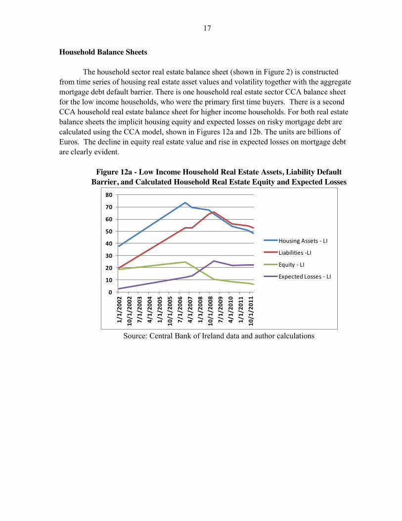
The household sector real estate balance sheet (shown in Figure 2) is constructed from time series of housing real estate asset values and volatility together with the aggregate mortgage debt default barrier. There is one household real estate sector CCA balance sheet for the low income households, who were the primary first time buyers. There is a second CCA household real estate balance sheet for higher income households. For both real estate balance sheets the implicit housing equity and expected losses on risky mortgage debt are calculated using the CCA model, shown in Figures 12a and 12b. The units are billions of Euros. The decline in equity real estate value and rise in expected losses on mortgage debt are clearly evident.

Figure 12a - Low Income Household Real Estate Assets, Liability Default

Barrier, and Calculated Household Real Estate Equity and Expected Losses

Source: Central Bank of Ireland data and author calculations

0

10

20

30

40

50

60

70

80

1/1

/20

02

10

/1/2

00

2

7/1

/20

03

4/1

/20

04

1/1

/20

05

10

/1/2

00

5

7/1

/20

06

4/1

/20

07

1/1

/20

08

10

/1/2

00

8

7/1

/20

09

4/1

/20

10

1/1

/20

11

10

/1/2

01

1

Housing Assets - LI

Liabilities -LI

Equity - LI

Expected Losses - LI

18

Figure 12b - High Income Household Real Estate Assets, Liability Default Barrier, and Calculated Household Real Estate Equity and Expected Losses

Source: Central Bank of Ireland and author calculations

The household “parent” balance sheet assets are calculated using the equity in

household real estate (the sum of the equity of low income and high income groups), disposable income, and financial assets (bn Euros). Note the sharp decline in household equity since 2007, decline in financial assets from 2007 to 2009, and decline in disposable income.

Figure 13 – Household Real Estate Equity, Income, Financial Assets and Consumption

Source: Central Bank of Ireland data and author calculations

0

50

100

150

200

250

300

350

400

450

1/1

/20

02

11

/1/2

00

2

9/1

/20

03

7/1

/20

04

5/1

/20

05

3/1

/20

06

1/1

/20

07

11

/1/2

00

7

9/1

/20

08

7/1

/20

09

5/1

/20

10

3/1

/20

11

1/1

/20

12

Housing Assets - HI

Liabilities -HI

Equity - HI

Expected Losses - HI

0

50

100

150

200

250

300

350

400

1/1

/20

02

11

/1/2

00

2

9/1

/20

03

7/1

/20

04

5/1

/20

05

3/1

/20

06

1/1

/20

07

11

/1/2

00

7

9/1

/20

08

7/1

/20

09

5/1

/20

10

3/1

/20

11

1/1

/20

12

Household Equity

Fin assets

Disp Income

Household Consumption

19

Commercial Real Estate (CRE) and Corporate Sector Risk Commercial real estate property prices rose until 2007 but declined by 70 percent by

2012 as shown in Figure 14.

Figure 14 – Commercial Property Prices in Ireland (index)

Some rough data on commercial real estate debt plus property price and other data allowed an approximate CCA balance sheet to be constructed and expected losses estimated.

For the corporate sector Moody’s CreditEdge gives market capitalization, market value of assets, and default probabilities and spreads from a CCA model. Using the average corporate sector default probabilities and spreads plus balance sheet data, expected losses can be estimated as shown in Table 1. Banking exposure data is not available but only two or three of listed corporates are in the real estate or construction sector. Corporate sector firms are mostly in services, high tech, energy companies, etc. The loss estimates are low. However aggregating the values of all listed firms is a problem as it averages out the expected losses. As a rough approximation it will be assumed banks are exposed to have of these (modest) losses.

Table 1 – Corporate Sector Market Capitalization, Assets and Expected Losses (3 yr horizon, Billion Euros)

2009 2010 2011

Market Capitalization 81.4 120.0 122.5 Market Value of Assets 139.8 192.7 190.9 Expected Losses 13.2 6.6 4.8

0

50

100

150

200

250

1/1

/20

02

7/1

/20

02

1/1

/20

03

7/1

/20

03

1/1

/20

04

7/1

/20

04

1/1

/20

05

7/1

/20

05

1/1

/20

06

7/1

/20

06

1/1

/20

07

7/1

/20

07

1/1

/20

08

7/1

/20

08

1/1

/20

09

7/1

/20

09

1/1

/20

10

7/1

/20

10

1/1

/20

11

7/1

/20

11

1/1

/20

12

20

Expected Losses Transferred to Banks, Market Implied Guarantees, and Actual Costs To get an estimate of the risk transmission to the banking sector the sum of expected losses from the household sectors, corporate sector, and commercial real estate loans is calculated (a three year horizon is used, the date is February 2009).6 The total expected losses are around 43 billion Euros. This compares to actual reported banking system losses of around 46 billion Euros post crisis estimates (see Figure 16 from Central Bank of Ireland). The market implied government contingent liabilities as early 2009 are 52 billion Euros (the peak level before Anglo was taken over). These estimates are shown in Figure 15. So expected losses transferred to the banks is close to the actual losses paid for by the government. The peak contingent liability estimates in January-February 2009 are slightly higher than the actual (post-crisis) estimate of losses paid for by the government. Implied sovereign assets were estimated to be 80 billion Euros in early 2009. The actual losses are thus 57 percent of the sovereign asset estimate.

Figure 15 - Comparison of Expected Losses from HH, CRE, and Corporates to Contingent Liability Estimates and to Actual Banking Losses Paid by Government

Sources: Author estimates, CreditEdge, Central Bank of Ireland data

6 A three year horizon is common in stress testing, three year horizon was used for loss calculations by Black Rock in the stress tests.

0

10

20

30

40

50

60

Commercial RE Expected

Losses

Household Expected

Losses

Total HH, CRE and Corp Expected

Losses

Market Implied Government Guarantee to

Banking System

Actual Banking Losses Paid for

by Irish

Government

21

Figure 16 – Central Bank of Ireland Reported Cost of Banking Crisis

Source: Central Bank of Ireland Macro-Financial Review 2013:1

22

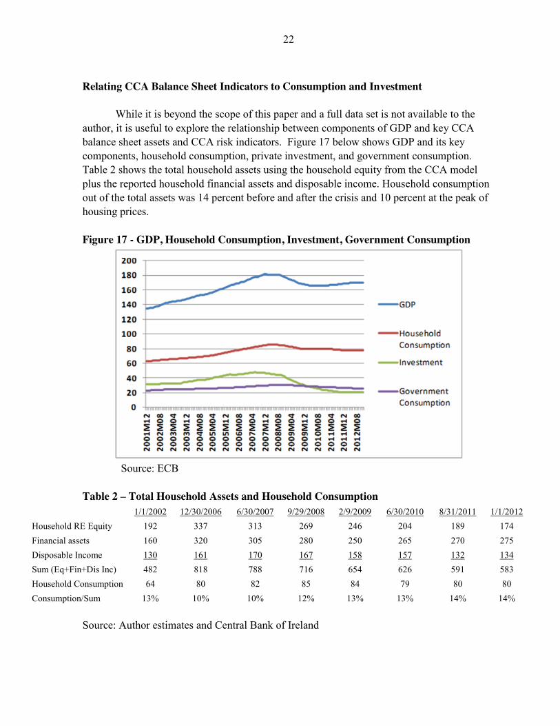
Relating CCA Balance Sheet Indicators to Consumption and Investment While it is beyond the scope of this paper and a full data set is not available to the author, it is useful to explore the relationship between components of GDP and key CCA balance sheet assets and CCA risk indicators. Figure 17 below shows GDP and its key components, household consumption, private investment, and government consumption. Table 2 shows the total household assets using the household equity from the CCA model plus the reported household financial assets and disposable income. Household consumption out of the total assets was 14 percent before and after the crisis and 10 percent at the peak of housing prices. Figure 17 - GDP, Household Consumption, Investment, Government Consumption

Source: ECB Table 2 – Total Household Assets and Household Consumption

1/1/2002 12/30/2006 6/30/2007 9/29/2008 2/9/2009 6/30/2010 8/31/2011 1/1/2012

Household RE Equity 192 337 313 269 246 204 189 174 Financial assets 160 320 305 280 250 265 270 275 Disposable Income 130 161 170 167 158 157 132 134 Sum (Eq+Fin+Dis Inc) 482 818 788 716 654 626 591 583 Household Consumption 64 80 82 85 84 79 80 80 Consumption/Sum 13% 10% 10% 12% 13% 13% 14% 14%

Source: Author estimates and Central Bank of Ireland

23

When household assets are higher, consumption is higher. A simple regression shows that household consumption = 0.0383*total household assets. From 2002 to peak housing prices in 2007 household assets rose 63% and household consumption rose 29%. From 2007 to 2012 household assets fell 26% and consumption fell 3%. Understanding the behavior of investment is complex. There is some indication corporate default risk is related to investment trends but more information on investment related to real estate and non-real estate corporate investment is necessary. Further Work and Applications

This simple framework illustrates the value of risk adjusted balance sheets and ways to measure risk transmission at the sector level. More disaggregation and detailed exposure data of banks could improve the framework. It could be adapted to analysis of stress scenarios for banks and government with feedbacks to and from households, real estate prices and components of GDP. It could be adapted to analyze counterfactual policies. If there had been a policy of countercyclical capital buffers, mandatory subordinated debt for banks or raising loan to value (LTV) ratios in the property boom period how might this have slowed the rise in house and commercial real estate value and moderated the boom and help smooth out GDP. Higher LTV ratios would have to have been put in place early on, such as in 2005. This model illustrates the disastrous fiscal consequences of the blanket guarantee for bank liabilities. More work could be done on household refinancing (as in Khandani et al. 2009).

In terms of relating the CCA risk indicators to components of GDP there are a number of alternatives using econometric models. CCA risk indicators for corporate, banking sector and sovereign have been included in Global VAR models (see Gray et al 2013). For a single country the time series of the CCA risk indicators could be related to credit and components of GDP (investment, household consumption, and government consumption) using VAR models or factor augmented VAR (FAVAR) model.

24

Appendix 1 Contingent Claims Analysis We can use this basic idea to construct risk-adjusted balance sheets, i.e. CCA balance

sheets where the total market value of assets, A, at any time, T, is equal to the sum of its equity market value, E, and its risky debt, D. The asset value is stochastic and may fall below the value of outstanding liabilities. Equity and debt derive their value from the uncertain assets. As pointed out by Merton (1973) equity value is the value of an implicit call option on the assets, with an exercise price equal to default barrier, B. The value of risky debt is equal to default-free debt minus the present value of expected loss due to default. The firm’s outstanding liabilities constitute the bankruptcy level. The expected loss due to default can be calculated as the value of a put option on the assets, A, with an exercise price equal to B, time horizon T, risk-free rate r, and, asset volatility

AV . The value of the implicit put option will

be called the Expected Loss Value (ELV).

Risky Debt = Default-free Debt − Expected Loss Value

rTD B e E L V

The calibration of the model uses the value of equity, the volatility of equity, the distress barrier as inputs into two equations in order to calculate the implied asset value and implied asset volatility.7 Equity and equity volatility are consensus forecasts of market participants and this provide forward-looking information. The value of assets is unobservable, but it can be implied using CCA. In the Merton Model for firms, banks and non-bank financials with traded equity use equity, E, and equity volatility,

EV , and the

distress barrier in the following two equations (equations 18 and 19) to solve for the two unknowns A, asset value, and

AV , asset volatility. ( )N is the cumulative standard normal

distribution. 1 2N ( ) N ( )rTE A d B e d

1

( )E A

E A N dV V

1

2

ln2

A

A

Ar

Bd

T

TV

V

§ ·§ ·¨ ¸ ¨ ¸© ¹ © ¹ and 2

2

ln2

A

A

Ar

Bd

T

TV

V

§ ·§ ·¨ ¸¨ ¸

© ¹ © ¹

Once the asset value, asset volatility are known, together with the default barrier, time horizon, and r, the values of the ELV (implicit put option) are calculated from: 7 See Merton (1973, 1974, 1977, 1992), Gray, Merton, and Bodie (2008), and Gray and Malone (2008).

25

2 0 1(( ) )rTE L V A N dB e N d

Risk-neutral probability of default is 2( )N d .

The formula for the credit spread is:

1 ln (1 )Ts E L and the 2( ) *rT

E L VE L N d L G D

B e

Moody’s CreditEdge calculates the Fair Value CDS (FVCDS), which is calculated using an LGD that is the average LGD for the banking sector as a whole.

1

ln 1 r isk n e u tra lF V C D S C E D F L G DT

The expected loss ratio is: risk n eu tra lC E D F L G D E L

26

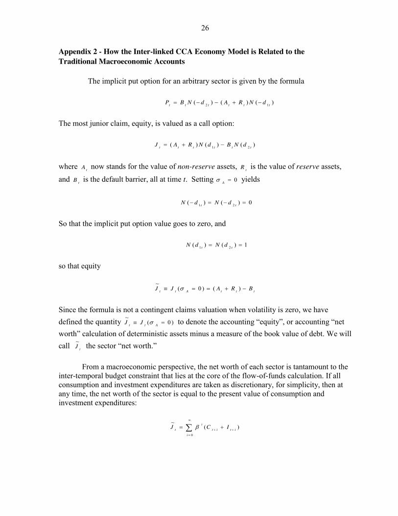
Appendix 2 - How the Inter-linked CCA Economy Model is Related to the Traditional Macroeconomic Accounts

The implicit put option for an arbitrary sector is given by the formula

)()()( 12 tttttt dNRAdNBP

The most junior claim, equity, is valued as a call option:

)()()( 21 tttttt dNBdNRAJ where tA now stands for the value of non-reserve assets, tR is the value of reserve assets, and tB is the default barrier, all at time t. Setting 0 AV yields

0)()( 21 tt dNdN

So that the implicit put option value goes to zero, and

1)()( 21 tt dNdN

so that equity

tttAtt BRAJJ )()0(~

V Since the formula is not a contingent claims valuation when volatility is zero, we have defined the quantity )0(

~ Att JJ V to denote the accounting “equity”, or accounting “net

worth” calculation of deterministic assets minus a measure of the book value of debt. We will call tJ

~ the sector “net worth.”

From a macroeconomic perspective, the net worth of each sector is tantamount to the inter-temporal budget constraint that lies at the core of the flow-of-funds calculation. If all consumption and investment expenditures are taken as discretionary, for simplicity, then at any time, the net worth of the sector is equal to the present value of consumption and investment expenditures:

¦f

0

)(~

iitit

it ICJ E

27

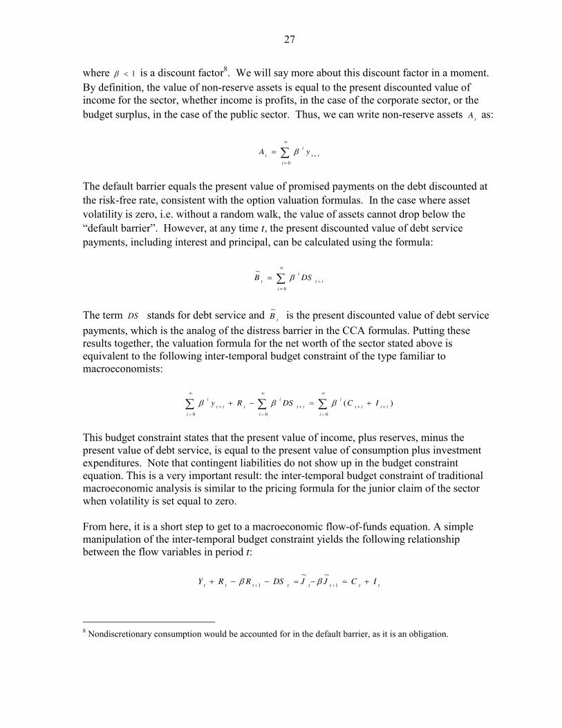
where 1E is a discount factor8. We will say more about this discount factor in a moment. By definition, the value of non-reserve assets is equal to the present discounted value of income for the sector, whether income is profits, in the case of the corporate sector, or the budget surplus, in the case of the public sector. Thus, we can write non-reserve assets tA as:

¦f

0i

iti

t yA E

The default barrier equals the present value of promised payments on the debt discounted at the risk-free rate, consistent with the option valuation formulas. In the case where asset volatility is zero, i.e. without a random walk, the value of assets cannot drop below the “default barrier”. However, at any time t, the present discounted value of debt service payments, including interest and principal, can be calculated using the formula:

¦f

0

~

iit

it DSB E

The term DS stands for debt service and tB~ is the present discounted value of debt service

payments, which is the analog of the distress barrier in the CCA formulas. Putting these results together, the valuation formula for the net worth of the sector stated above is equivalent to the following inter-temporal budget constraint of the type familiar to macroeconomists:

¦¦¦f

f

f

000

)(i

ititi

iit

it

iit

i ICDSRy EEE

This budget constraint states that the present value of income, plus reserves, minus the present value of debt service, is equal to the present value of consumption plus investment expenditures. Note that contingent liabilities do not show up in the budget constraint equation. This is a very important result: the inter-temporal budget constraint of traditional macroeconomic analysis is similar to the pricing formula for the junior claim of the sector when volatility is set equal to zero.

From here, it is a short step to get to a macroeconomic flow-of-funds equation. A simple manipulation of the inter-temporal budget constraint yields the following relationship between the flow variables in period t:

tttttttt ICJJDSRRY 11

~~EE

8 Nondiscretionary consumption would be accounted for in the default barrier, as it is an obligation.

28

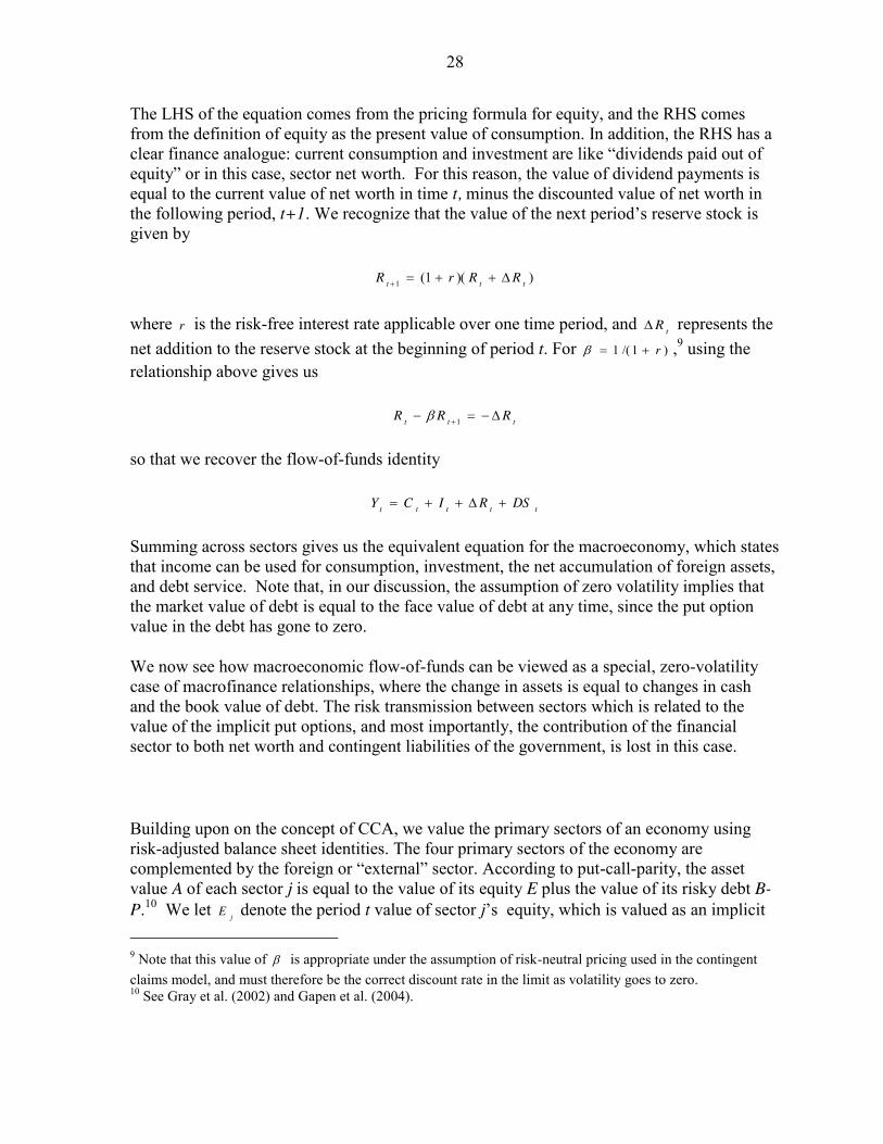
The LHS of the equation comes from the pricing formula for equity, and the RHS comes from the definition of equity as the present value of consumption. In addition, the RHS has a clear finance analogue: current consumption and investment are like “dividends paid out of equity” or in this case, sector net worth. For this reason, the value of dividend payments is equal to the current value of net worth in time t, minus the discounted value of net worth in the following period, t+1. We recognize that the value of the next period’s reserve stock is given by

))(1(1 ttt RRrR '

where r is the risk-free interest rate applicable over one time period, and tR' represents the net addition to the reserve stock at the beginning of period t. For )1/(1 r E ,9 using the relationship above gives us

ttt RRR ' 1E

so that we recover the flow-of-funds identity

ttttt DSRICY '

Summing across sectors gives us the equivalent equation for the macroeconomy, which states that income can be used for consumption, investment, the net accumulation of foreign assets, and debt service. Note that, in our discussion, the assumption of zero volatility implies that the market value of debt is equal to the face value of debt at any time, since the put option value in the debt has gone to zero.

We now see how macroeconomic flow-of-funds can be viewed as a special, zero-volatility case of macrofinance relationships, where the change in assets is equal to changes in cash and the book value of debt. The risk transmission between sectors which is related to the value of the implicit put options, and most importantly, the contribution of the financial sector to both net worth and contingent liabilities of the government, is lost in this case.

Building upon on the concept of CCA, we value the primary sectors of an economy using risk-adjusted balance sheet identities. The four primary sectors of the economy are complemented by the foreign or “external” sector. According to put-call-parity, the asset value A of each sector j is equal to the value of its equity E plus the value of its risky debt B-P.10 We let jE denote the period t value of sector j’s equity, which is valued as an implicit 9 Note that this value of E is appropriate under the assumption of risk-neutral pricing used in the contingent claims model, and must therefore be the correct discount rate in the limit as volatility goes to zero. 10 See Gray et al. (2002) and Gapen et al. (2004).

29

call option, and jD denote the value of risky debt, which is equal to the default-free value

iB ( rT

i iB B e ), minus the value of the implicit put option, which is denoted by jP and measures the expected losses associated with the debt. Then put-call-parity relationships for the four domestic sectors can be written as follows. For the corporate sector (C), assets CA equal equity CE plus the risky debt ( )C CB P :

( )C C C CA E B P

For the financial sector (F), assets FA plus contingent financial support from the sovereign

FPD equals equity, FE , plus the value of risky debt and deposits, (1 )F FB PD , so that

( (1 ) )F F F F FA P E B PD D

Here FP is the implicit put option to the financial sector.11 The value of the sovereign guarantee is a fraction D of the financial sector expected loss FP , and the remainder,(1 ) FPD measures the residual expected loss of secured debt and deposits of the financial sector.

For the sovereign, assets SA include foreign currency reserves, M AR , the net fiscal asset GA (=( )P V T G , present value of taxes minus government expenditures) and other public assets

O th erA . The net fiscal asset is defined as the present value of taxes and revenues, including seigniorage, minus the present value of government expenditures. GE is “equity” of the government of which GET is the portion which is credit from the monetary authorities and is junior to debt obligations. The liabilities of the sovereign include base money B MM , risky local-currency debt S L C S L CB P , risky foreign-currency debt S F X S F XB P , and financial guarantees/contingent liabilities FPD as shown below:

( ) ( )S M A G O th e r B M S L C S L C S F X S F X FA R A A M B P B P PD

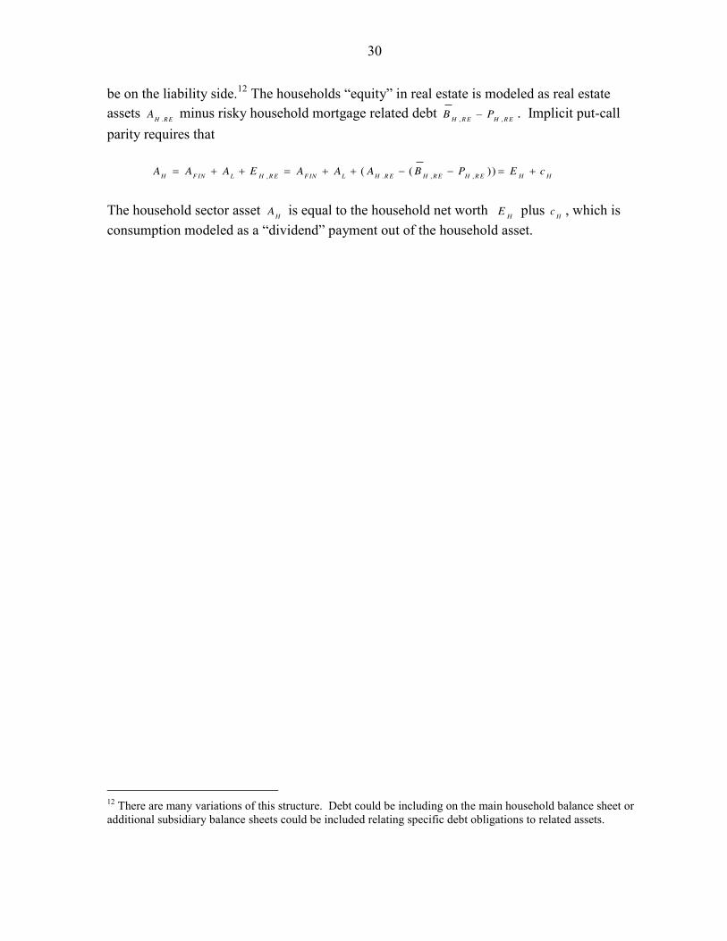
For the household sector, asset HA is the sum of the household sector’s financial wealth F INA , the present value of its labor income LA , and equity ,H R EE in real estate. The debt of households to banks and non-banks is frequently tied to homes and real estate. For this reason it is practical to have two segregated but linked household CCA balance sheets. The “subsidiary” balance sheet would have real estate as the primary asset and related debt would 11 Merton (1977) was the first to demonstrate that the government’s guarantee to banks could be modeled as an implicit put option.

30

be on the liability side.12 The households “equity” in real estate is modeled as real estate assets .H R EA minus risky household mortgage related debt , ,H R E H R EB P . Implicit put-call parity requires that

, . , ,( ( ))H F IN L H R E F IN L H R E H R E H R E H HA A A E A A A B P E c

The household sector asset HA is equal to the household net worth HE plus Hc , which is consumption modeled as a “dividend” payment out of the household asset.

12 There are many variations of this structure. Debt could be including on the main household balance sheet or additional subsidiary balance sheets could be included relating specific debt obligations to related assets.

31

References

Black F. and M, Scholes, 1973, “The Pricing of Options and Corporate Liabilities,” J. Polit. Econ. 81(3):637–54

Central Bank of Ireland, Macro-Financial Review 2012:1, 2012:2, 2013:1, FMP program and website data.

Gapen M.T., Gray D.F., Lim C.H. and Y. Xiao, 2005, “Measuring and Analyzing Sovereign Risk with Contingent Claims,” IMF Work. Paper 05/155. Washington, DC: Int. Monet. Fund.

Gapen, M. 2009 "Evaluating the Implicit Guarantee to Fannie Mae and Freddie Mac Using Contingent Claims," in Credit, Capital, Currency, and Derivatives: Instruments of Global Financial Stability or Crisis? International Finance Review, volume 10, forthcoming 2009.

Gray, D 2009 “Modeling Financial Crises and Sovereign Risk” Annual Review of Financial Economics (edited by Robert Merton and Andrew Lo). Annual Reviews, Palo Alto California, USA.

Gray, D., M. Gross, J. Paredes, M. Sydow, 2013, “Modeling Banking, Sovereign, and Macro Risk in CCA Global VAR” , IMF Working Paper 13/218, Washington D.C.

Gray, D. F., and A. A. Jobst, 2013, “Systemic Contingent Claims Analysis –Estimating

Market-Implied Systemic Risk” IMF Working Paper 13/54 (Washington: International Monetary Fund).

Gray, D. and S. Malone, 2012, “Sovereign and Financial Sector Risk: Measurement and Interactions” Annual Review of Financial Economics, 4:9.

Gray, D., A. Jobst, 2011, “Modeling Systemic Financial Sector and Sovereign Risk,” Sveriges Riksbank Economic Review, September.

Gray, D., and A. A. Jobst, 2010, “New Directions in Financial Sector and Sovereign Risk Management” JOIM, Vol. 8, No.1, pp.23-38.

Gray D, and S. Malone. 2008. Macrofinancial Risk Analysis. Foreword by RC Merton. New York: Wiley

Gray, D. F., Jobst, A. A., and S. Malone, 2010, “Quantifying Systemic Risk and Reconceptualizing the Role of Finance for Economic Growth,” Journal of Investment Management, Vol. 8, No. 2, pp. 90-110.

32

____________________________________2011, “Sovereign debt, banking sector vulnerability, and dynamic risk spillovers in Europe,” EC Conference Public Debt and Growth Brussels, Belgium, December 2010

Gray DF, Merton RC, Bodie Z. 2002. A new framework for analyzing and managing macrofinancial risks. Presented at Conf. Finance Macroecon., NY Univ., New York, Oct.

Gray DF, Merton RC, Bodie Z. 2007a. New framework for measuring and managing macrofinancial risk and financial stability. NBER Work. Pap. No. 13607

Gray DF, Merton RC, Bodie Z. 2007b. Contingent claims approach to measuring and managing sovereign credit risk. J. Invest. Manag. 5(4)5--28 (Spec. Issue Credit Anal.)

Gray DF, Merton RC, Bodie Z. 2008. New framework for measuring and managing macrofinancial risk and financial stability. Harvard Bus. Sch. Work. Pap. No. 09-015 (Revised)

Khandani, A, Lo, A.W. and R. C. Merton, 2009, “Systemic Risk and the Refinancing Ratchet Effect,” Harvard Business School, Working paper, pp. 36f.

KMV, 2001. Modeling Default Risk, KMV Corp.

Merton RC. 1973. Theory of rational option pricing. Bell J. Econ. Manag. Sci., 4(Spring):141–83

Merton RC. 1974. On the pricing of corporate debt: The risk structure of interest rates. J. Finance 29(May):449--70

Merton RC. 1977. An analytic derivation of the cost of loan guarantees and deposit insurance: An application of modern option pricing theory. J. Bank. Finance 1:3–11

Merton RC. 1992. Continuous-time Finance. Oxford, UK: Basil Blackwell. Rev. ed.

Merton RC. 1998. Applications of option-pricing theory: Twenty-five years later. Les Prix Nobel 1997, Stockholm: Nobel Found. Reprinted in Am. Econ. Rev. 88(June): 323-49

Merton RC, Bodie Z. 1992. On the management of financial guarantees. Financ. Manag. 21(Winter):87–109

Merton, Robert C., Monica Billio, Mila Getmansky, Dale Gray, Andrew W. Lo, and Loriana Pelizzon, 2013, “On a New Approach for Analyzing and Managing Macrofinancial Risks,” Financial Analysts Journal, vol 69, no 2.

33

Whelan, Karl, 2013, “Ireland’s Economic Crisis: The Good, Bad and the Ugly” Presented at the Bank of Greece conference on the Euro Crisis, Athens May 24, 2013.