Analyzing the Effects of a Merger between Airline Codeshare Partners

Dave Brown* and Philip G. Gayle**

March 2009

Abstract In October 2008, the Department of Justice approved the Delta/Northwest merger, claiming the potential for substantial cost efficiencies with little or no harmful effects on competition. What makes this merger particularly interesting is that Delta and Northwest are codeshare partners. As such, the merger could have varying effects across different product types (pure online versus codeshare). Using pre-merger data and a structural econometric model, we analyze the potential effects of this merger. We find that predicted percent price increases for Delta and Northwest codeshare products are larger than the predicted percent increases for their pure online products. Keywords: Merger Analysis; Codeshare Alliance; Airline Competition JEL Classification codes: L13, L93, C1, C25 Acknowledgement: We thank Jaime Brown for collecting data on population. We also thank Robert Porter, Dennis Weisman, and Tian Xia for helpful comments and suggestions. *Kansas State University, Department of Economics, 327 Waters Hall, Manhattan, KS 66506; email: dbrown3@ksu.edu. **Kansas State University, Department of Economics, 320 Waters Hall, Manhattan, KS 66506; (785) 532-4581; Fax:(785) 532-6919; email: gaylep@ksu.edu; corresponding author.

1

1. Introduction

Market power is often studied in the microeconomic literature for various reasons.

Industries with high concentration ratios tend to have higher markups and profits due to the

firms’ ability to set higher prices. Of particular interest in this field are mergers and their effects.

When a merger occurs, the market will become more concentrated, but the effects aren’t always

the same – a merger could be harmful by greatly decreasing competition, increasing prices, and

heightening entry barriers. However, a merger may also create cost efficiencies – if costs

decrease for a firm, lower prices may follow, which can be beneficial for competition.

Although there was much speculation as far back as February 2008 about a possible

merger between the two firms,1 Delta officially announced its plans to acquire Northwest on

April 14, 2008.2 The combined carrier plans to operate under the Delta name, be headquartered

in Atlanta, and operate the nine hubs of both airlines in the U.S., Europe, and Asia.

Critics believe that the merger will cause significant price increases and may even initiate

other large airline mergers, eventually leading to an industry with less than 5 main competitors.

On May 14th, 2008, Minnesota Democratic Congressman James Oberstar stated that “This

should not be and must not be considered a standalone, individual transaction but rather as the

trigger of what will surely be a cascade of subsequent mergers that will consolidate aviation in

the United States and around the world into global, mega carriers.”3 If true, this (according to

microeconomic theory) could lead to higher markups and prices if market power could be

exercised.

1 Atlanta Journal-Constitution. http://www.ajc.com/business/content/business/delta/stories/2008/02/16/delta_0217.html 2 CNN Money. http://money.cnn.com/2008/04/14/news/companies/delta_northwest/index.htm 3 CNN Money. http://money.cnn.com/2008/05/14/news/companies/airline_merge/index.htm?postversion=2008051418

2

Proponents, specifically the airlines, must show that the merger will have positive effects,

and that the positive effects will outweigh any negative effects such as price increases. If two

firms wanting to merge can show benefits of the merger – such as cost efficiencies and increased

quality of service – the merger has a greater chance of getting approved by the U.S. Department

of Justice (DoJ).4

On August 6th, 2008, the European Commission gave unconditional clearance for the

merger. The Commission stated that the merger would not impede effective competition in

Europe or the trans-Atlantic. Further, a new development occurred less than two months later on

September 25th when the stockholders of the two companies “overwhelmingly approved” the

merger. 5 After the shareholders approved, the legal processes continued, and it was up to the

DoJ to examine the situation to see if the merger would be permitted.

On October 29th, 2008, the DoJ approved the Delta/Northwest merger, stating that “the

Division has determined that the proposed merger between Delta and Northwest is likely to

produce substantial and credible efficiencies that will benefit U.S. consumers and is not likely to

substantially lessen competition”.6 Now that the merger is approved, the airlines can begin to

integrate. The integration process will take place over a period of 12 – 24 months, beginning in

early 2009.7

We use a well-known structural econometric framework8 to estimate the potential market

effects of the imminent Delta/Northwest merger in markets where their services overlap prior to

the merger. Specifically, we use pre-merger data to estimate demand, then use the demand 4 DoJ Horizontal Merger Guidelines. http://www.usdoj.gov/atr/public/guidelines/horiz_book/4.html 5 Delta Press Release http://news.delta.com/article_display.cfm?article_id=11162 6 Department of Justice Press Release http://www.usdoj.gov/atr/public/press_releases/2008/238849.htm 7 Delta Press Release http://news.delta.com/article_display.cfm?article_id=11176 8 For examples, see Nevo (2000) and Ivaldi and Verboven (2005).

3

parameter estimates along with an assumed price-setting behavior (Bertrand-Nash) of airlines to

recover product-level marginal costs. With the product-level marginal costs and demand

estimates in hand, we use the multiproduct firm Bertrand-Nash pricing framework to conduct

counterfactual experiments. One counterfactual experiment we ran is to compute the extent to

which Delta and Northwest product prices might increase in the worst case scenario in which the

merger does not produce any efficiency gains.

This merger is of particular interest because Delta and Northwest are codeshare partners.

With codesharing, a trip is ticketed by a single carrier, even though some (or all) of the flights on

the passenger itinerary are operated by a different carrier, which is the codeshare partner. This is

different from a pure online flight itinerary, in which the trip is ticketed and operated by the same

carrier. 9

There is a growing body of literature that analyzes airline mergers and the effects they

have on market power and airline fares. Beutel and McBride (1992) illustrate a direct

econometric method to estimate the change in market power caused by a merger. Their results

show that a merger may have very different quantitative effects for the firms involved based on

pre-merger market power. Singal (1996) studies the pricing behavior of airlines following

mergers that occurred in the 1980’s. Morrison (1996) uses a unique dataset to analyze long term

trends and effects of mergers by looking 7 years before and after a merger occurs, paying special

attention to routes that were served by both carriers before the merger. For the three mergers

studied, fares for the newly merged firm increased immediately after the merger, but fell over

time to levels at or below competitors’ fares. Competition on the routes was always higher prior

to the mergers. Clougherty (2006) studies domestic mergers, but argues that these mergers are

driven by international competition incentives as well as domestic competition incentives. He 9 Formal definitions of codeshare and pure online products are given in Section 2.

4

finds that domestic mergers lead to an increased international competitive performance due to

network enhancement and network consolidation effects. Peters (2006) uses a counterfactual

simulation method similar to ours in order to predict price increases resulting from five airline

mergers that occurred in the 1980s, and compares the predicted price increases to actual price

increases. The post-merger data allowed differences in predicted price changes and actual price

changes to be decomposed. He finds that unobservable supply-side factors, namely changes in

marginal costs and deviations from the assumed model of firm conduct, play a large role in post-

merger price increases.

Other literature has studied the effects of alliances, but with the exception of Ito and Lee

(2007) and Gayle (2008), these studies do not address the different types of products associated

with codesharing. Adler and Smilowitz (2007) demonstrate a basic framework assuming

competitive markets and minimal regulation that allows airlines to choose both international

network structure and alliances. They find that both alliances and mergers have a positive effect

for partners involved but damaging effects for an airline that fails to find an alliance or merger

partner.

Finally, there is a relatively small portion of the literature that explicitly analyzes

codesharing. Bilotkach (2007) examines airline consolidation (defined as forming an alliance

and codesharing) using transatlantic markets to inspect if codesharing with and without antitrust

immunity decreases fares for interline trips equally. The results show that codesharing and

alliance-forming both have fare-decreasing effects, but the codesharing effect is more than twice

the magnitude of the alliance effect. As noted in Brueckner and Whalen (2000) and Brueckner

(2003), codesharing allows airlines to eliminate a double markup on itineraries with multiple

5

operators, resulting in lower fares. Ito and Lee (2007) also show codesharing to be associated

with lower fares.

This paper analyzes potential market effects of the Delta/Northwest merger with a

particular focus on comparing predicted price changes across different product types (codeshare

vs. pure online). To the best of our knowledge, our paper is the first to examine the potential

market effects across different product types of an airline merger between codeshare alliance

partners.

The data reveal that Delta and Northwest products are substitutable (competing) in a

significant number of markets in which they offer products. Delta offers products in over half of

the markets in which Northwest offers products, and Northwest offers products in almost half of

the markets in which Delta offers products. Thus, antitrust authorities clearly should not grant

approval of the merger on the grounds that these carriers rarely compete. Deeper analysis is

required to assess the extent to which: (1) these two carriers constrain each other’s pricing

decisions when they compete; (2) other competing carriers would constrain the joint pricing

behavior of Delta and Northwest. To get at these issues we use our econometric model to predict

the extent to which Delta and Northwest’s product prices will increase if these products are

jointly priced in the worst case scenario where the merger is not associated with cost efficiency

gains.

In our sample, Delta and Northwest have a combined 28.95% passenger share in the U.S.

domestic industry, varying between 0.58% to 100% in different markets. Based on our

econometric estimates, the average predicted change in price due to the merger is only an

increase of 0.54%, hardly big enough to concern consumers, let alone antitrust authorities. The

6

mean predicted price increase among Delta/Northwest products is 1.45% – however, the

maximum predicted increase in price was over 13%.

To better understand predicted percent price increases for Delta and Northwest products

(which varied across markets and product types), we ran auxiliary regressions with predicted

percent price increases as the dependent variable and various product and market characteristics

as regressors. The results reveal a significant positive relationship between the share of

Delta/Northwest passengers in a market and the predicted increase in prices attributed to the

merger. We also find that Delta/Northwest codeshare products have higher predicted price

increases relative to their pure online products.

Finally, we analyzed competition at the market level (rather than product level) to

examine market level factors that influence the predicted price increases. We find that the

presence of other airlines offering competing products is crucial in keeping the predicted price

increases of Delta/Northwest products low.

The rest of the paper is as follows: Section 2 outlines the model while Section 3 details

the estimation. Section 4 discusses the data, the results are covered in Section 5, and Section 6

offers concluding remarks.

2. The Model

Definitions

A couple of definitions are worth mentioning before illustrating the model. These

definitions follow from Gayle (2007a and 2008). A market is defined as an origin-destination

combination. Markets are directional, meaning that a trip from Los Angeles to New York is a

different market than a trip from New York to Los Angeles. This allows us to consider origin

7

city characteristics such as population and whether or not the airport is a hub for the carrier

offering the air travel product for sale.

An itinerary contains the origin and destination of the journey, as well as all of the

intermediate stops. Thus, a non-stop flight from Chicago to Seattle is a different itinerary than a

passenger who flies from Chicago to Seattle with a layover in Denver. A product is defined as a

combination of airline(s) and itinerary. Each flight has a ticketing carrier and an operating

carrier. The ticketing carrier is the airline that actually sells the flight ticket to the passenger and

is the ‘owner’ of the product. The operating carrier is the airline that owns the plane that the

passenger is traveling on for the flight.

Further, we want to study the effects of a merger on codeshared products relative to pure

online products. While all flights have both an operating carrier and ticketing carrier, the

ticketing carrier and operating carrier could be the same or different for any flight on the

itinerary. A pure online product has a single ticketing carrier and operating carrier for the whole

itinerary and the two carriers are the same. For example, a passenger buys a single ticket from

United and flies on two United planes for his itinerary. A traditional codeshare product has a

single ticketing carrier for the trip, but multiple operating carriers, one of which is the same as

the ticketing carrier. For example, a single ticket is purchased from Delta for a two-flight

itinerary where one of the planes is a Delta plane and the other is a Continental plane. A virtual

codeshare product has a single ticketing carrier and operating carrier for the itinerary, but the

operating and ticketing carriers are different. For example, a single-flight itinerary is ticketed

through Northwest, but the passenger flies on a Continental plane.10

10 For a more detailed analysis of codesharing, see Gayle (2008), and Ito and Lee (2007).

8

Demand

We start out by estimating a discrete choice demand model in which a consumer chooses

one product among many alternatives with the goal of utility maximization. The consumer also

has the option to choose an outside alternative (driving, taking a train, or not traveling at all).

Specifically, we use a nested logit demand model. Let there be G groups of products and

one additional group for the outside good. Products within the same group are closer substitutes

than products from different groups. Groups are defined as an origin-destination-quarter

combination, so all inside products in a market belong to the same group. Let product j be in

group g. The utility of consumer i from purchasing product j is given by

ijigjiju εσζδ )1( −++= , (1)

where jδ is the mean valuation across consumers of product j, igζ is a random component of

utility that is common to all products in group g, σ measures the correlation of the consumers’

utility across products belonging to the same group, and ijε is an idiosyncratic error term. If σ

= 1, there is a perfect correlation of preferences for products within the same group and the

products are perfect substitutes. If σ = 0, there is no correlation of preferences. As long as σ is

between 0 and 1 inclusive, the model is consistent with utility maximization, and each consumer

i chooses the product j that maximizes his utility.

The mean valuation jδ depends on the price of the product ( jp ), observed product

characteristics ( jx ), and unobserved (by researchers) product characteristics ( jξ ):

jjjj px ξαβδ +−= , (2)

where β is a vector of parameters that measures the marginal utility of respective non-price

product characteristics, and α is the marginal utility of price.

9

The probability that a consumer chooses j is as follows:

∑ =−

−

+×

−= G

g g

g

g

jj

D

DD

s1

1

1

1

))1/(exp(σ

σσδ, (3)

where

[ ]∑∈

−=gGk

kgD )1/(exp σδ .

The choice probability coincides with the market share for the product.

The demand for product j is obtained by:

( )θ,,, ξpxjj sMd ×= , (4)

where M is a measure of the market size, which we assume to be the size of the population in the

origin city, ( )⋅js is the predicted product share function specified in equation (3), p and x are

vectors of observed price and non-price product characteristics respectively, ξ is a vector of

unobserved (by researchers) product characteristics, and ( )σβαθ ,,= is the vector of demand

parameters to be estimated.

Supply

Following the general procedure described in Nevo (2000), marginal costs are recovered

by using the estimated demand elasticities and assuming a model of pre-merger pricing conduct.

Then, we compute the new price equilibrium by using estimated demand, pre-merger marginal

costs, and assuming a model of post-merger pricing conduct. Finally, the predicted post-merger

equilibrium prices are compared to actual pre-merger prices.

Each firm f produces a set Ff of products. Firm f has a variable profit of

∑∈

−=fFj

jjjf qcp )(π , (5)

10

where ( )pjj dq = in equilibrium, jq is the quantity of tickets for product j sold in the market,

( )pjd is the market demand for product j specified in equation (4), p is a 1×J vector of product

prices, and jc is the marginal cost incurred from offering product j.

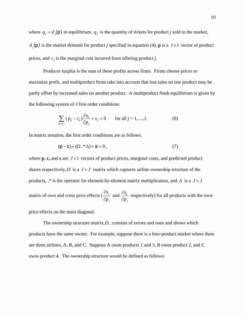
Producer surplus is the sum of these profits across firms. Firms choose prices to

maximize profit, and multiproduct firms take into account that lost sales on one product may be

partly offset by increased sales on another product. A multiproduct Nash equilibrium is given by

the following system of J first order conditions:

∑∈

=+∂∂

−fFk

jj

kkk s

pscp 0)( for all j = 1,…,J. (6)

In matrix notation, the first order conditions are as follows:

0)*. ()( =+ΔΩ×− scp , (7)

where p, c, and s are 1×J vectors of product prices, marginal costs, and predicted product

shares respectively,Ω is a JJ × matrix which captures airline ownership structure of the

products, .* is the operator for element-by-element matrix multiplication, and Δ is a JJ ×

matrix of own and cross price effects (j

j

ps∂∂

and j

k

ps∂∂ respectively) for all products with the own-

price effects on the main diagonal.

The ownership structure matrix,Ω , consists of zeroes and ones and shows which

products have the same owner. For example, suppose there is a four-product market where there

are three airlines, A, B, and C. Suppose A owns products 1 and 3, B owns product 2, and C

owns product 4. The ownership structure would be defined as follows:

11

⎥⎥⎥⎥

⎦

⎤

⎢⎢⎢⎢

⎣

⎡

=Ω

1000010100100101

.

If one airline owns all the products in a market, the ownership structure would be a JJ × matrix

of ones, with J being the number of products in the market.

Product markups are determined separately for each market. The markups for products in

any given market are:

scp ×ΔΩ−=−= −1)*. (markups . (8)

The counterfactual experiment involves specifying both a pre-merger and a post-merger

product ownership structure. First, marginal costs are recovered using the pre-merger product

ownership structure as follows:

spc ×ΔΩ+= −1)*. (ˆ pre , (9)

where c is the vector of estimated marginal costs for all products and preΩ is the pre-merger

product ownership structure. Now, assuming a post-merger product ownership structure of

postΩ and using pre-merger marginal costs, we can compute post-merger equilibrium prices by

searching for the new price vector *p that satisfies

[ ] spcp ×ΔΩ−=−1** )(*. ˆ post . (10)

Having solved for post-merger equilibrium prices *p , we can compare *p to p to see how the

merger would affect prices.11

Based on the ownership matrix preΩ , Delta and Northwest separately and independently

set the price of their products within a market for which each of them are the ticketing carrier.

11 Ivaldi and Verboven (2005) provide another application of this model by studying horizontal mergers approved by the European Commission.

12

This is true for all their product types – pure online, traditional codeshare, and virtual codeshare.

In the case of the postΩ ownership matrix, these Delta/Northwest products in the market are all

jointly priced by the new ticketing carrier formed by the merger of Delta and Northwest.

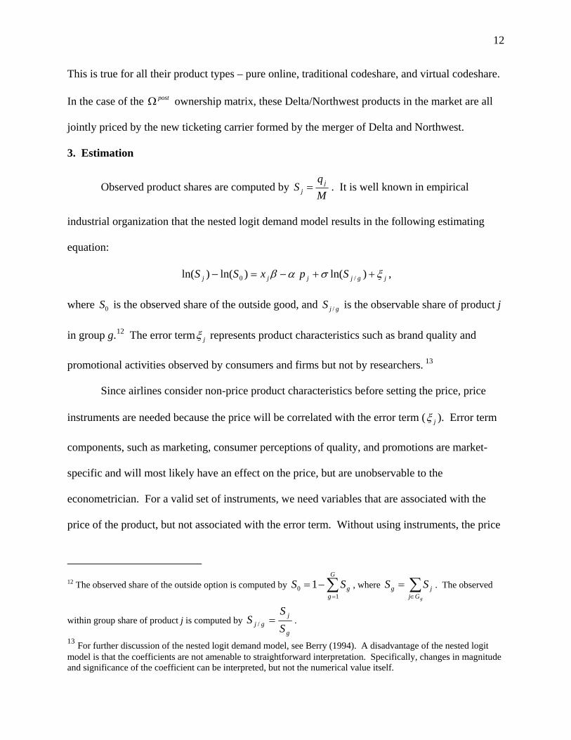
3. Estimation

Observed product shares are computed by Mq

S jj = . It is well known in empirical

industrial organization that the nested logit demand model results in the following estimating

equation:

jgjjjj SpxSS ξσαβ ++−=− )ln( )ln()ln( /0 ,

where 0S is the observed share of the outside good, and gjS / is the observable share of product j

in group g.12 The error term jξ represents product characteristics such as brand quality and

promotional activities observed by consumers and firms but not by researchers. 13

Since airlines consider non-price product characteristics before setting the price, price

instruments are needed because the price will be correlated with the error term ( jξ ). Error term

components, such as marketing, consumer perceptions of quality, and promotions are market-

specific and will most likely have an effect on the price, but are unobservable to the

econometrician. For a valid set of instruments, we need variables that are associated with the

price of the product, but not associated with the error term. Without using instruments, the price

12 The observed share of the outside option is computed by ∑

=

−=G

ggSS

10 1 , where ∑

∈

=gGj

jg SS . The observed

within group share of product j is computed by g

jgj S

SS =/ .

13 For further discussion of the nested logit demand model, see Berry (1994). A disadvantage of the nested logit model is that the coefficients are not amenable to straightforward interpretation. Specifically, changes in magnitude and significance of the coefficient can be interpreted, but not the numerical value itself.

13

coefficient estimated will be inconsistent. Further, gjS / is also endogenous, as non-price product

characteristics in jξ that affect the product price may also influence the within-group share of

the product.

Our instruments include the number of competitors in the market, the number of other

products offered by the airline, characteristics of competing products offered by competitors, and

the itinerary distance. Each of these instruments has an intuitive explanation for their inclusion.

For the competitors, supply theory predicts that a product’s price will be influenced by the

number and closeness of competitors in the market. Next, if an airline offers multiple products

in the same market, the airline will jointly set the prices for these products. When considering

other products, we examine competing products with the same number of intermediate stops and

similar levels of convenience. The more similarities there are between competing products, the

less discrepancy we expect between prices of these products. The inclusion of itinerary distance

is based on the idea that distance is correlated with marginal cost and therefore influences

price.14

When simple Two-Stage Least Squares (2SLS) is used to estimate the demand equation,

we find that the demand parameter estimates imply negative marginal cost for some products.

As such, we estimate demand using constrained Generalized Methods of Moments (GMM),

where the constraint is to impose non-negative marginal costs.

Constrained GMM Estimation

The constrained GMM estimation produces demand parameters that are consistent with

utility maximization and static profit maximization. Our demand estimation procedure requires

solving the following constrained optimization problem:

14 See Gayle (2007a) for similar types of instruments.

14

[ ])'()')('( 1 ξξθ

ZZZZMin −

such that 10 and ,0)min( <<≥− σmarkupp ,

where Z is the matrix of the control variables and instruments. The procedure minimizes the

objective function by choosing the set of parameters inθ . We use the 2SLS estimates as a

starting point for the GMM minimization procedure.

4. Data

Data are gathered from the DB1B market survey, published by the U.S. Department of

Transportation. This dataset is a quarterly 10% sample of all flight itineraries in the U.S. Each

observation in the dataset is a flight itinerary and includes information on operating and ticketing

carriers, fares, passengers, intermediate stops, total itinerary distance, origin and destination

airport, and the number of airports in the origin and destination city. Data was collected for four

quarters: 2007:2, 2007:3, 2007:4, and 2008:1. Only markets that appear in all four quarters and

include both Delta and Northwest itineraries are used for analysis. The data are further restricted

to include only itineraries in the contiguous U.S., and foreign operating carriers such as Air

France and Iberia are eliminated.15 Further, observations were dropped that listed market fares

less than $100 – this helps us avoid discounted fares that may be due to passengers using

frequent-flyer miles.

Collapsing the Data

Each quarter of data originally had over 5 million observations, making the data

extremely large and unmanageable. Due to the airlines being very effective at using yield

management, there are many identical itineraries that have different observed fares. This leads to

15 Eliminating the foreign airlines eliminated less than 600 observations in each quarter. Eliminating markets that flew to Alaska and Hawaii eliminated approximately 360,000 observations each quarter.

15

the dataset containing many repeat itineraries each listed as having passengers paying different

fares. To render our data more manageable, the dataset was collapsed by product – for each

quarter, passengers were aggregated over a given itinerary-airline(s) combination (this created

the quantity variable) and the average market fare was found, creating the price variable. In the

collapsed data set, each airline(s)-itinerary-quarter combination appears only once, with its

aggregated passenger quantity and average market fare.

Creation of Other Variables

From this collapsed dataset, observed product market shares jS are created. For the

purpose of properly identifying codeshare products in the data, feeder/regional operating carriers

are re-coded to match their major company.16 For example, Comair Delta Connection (OH) was

recoded as Delta (DL). Airline dummies are created, as well as indicators for whether the

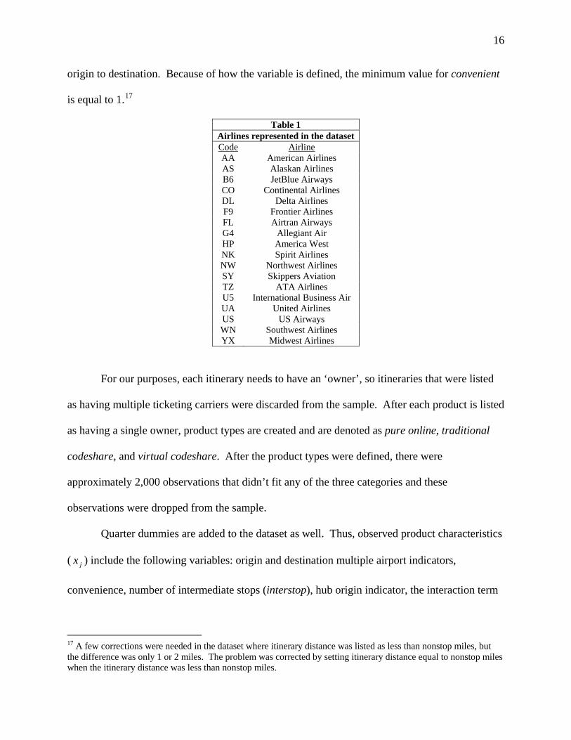
itinerary was pure online, traditional codeshared, or virtual codeshared. Ticketing carriers that

appeared less than 40 times were dropped – this eliminated about 20 smaller ticketing carriers

that appeared in the dataset. The final set of ticketing carriers is presented in Table 1. A dummy

variable hub_origin was created indicating whether the origin airport is a hub for the ticketing

carrier. This hub dummy variable was multiplied by the itinerary’s number of intermediate stops

to obtain an interaction variable hub_interstop.

A measure of product convenience is created as well, and is defined as itinerary distance

divided by nonstop miles, where nonstop miles is the direct flight distance between origin and

destination. Thus, the most convenient itinerary for a given market would be a direct flight from

16 We identify codeshare products as products where the ticketing and operating carriers differ. If we did not recode operating feeder carriers to have their major carrier code, then products that have the major carrier as the ticketing carrier and associated regional feeder carrier(s) as operating carrier(s) will mistakenly be counted as codeshare products since the operating and ticketing carrier codes would differ.

16

origin to destination. Because of how the variable is defined, the minimum value for convenient

is equal to 1.17

Table 1 Airlines represented in the dataset Code Airline AA American Airlines AS Alaskan Airlines B6 JetBlue Airways CO Continental Airlines DL Delta Airlines F9 Frontier Airlines FL Airtran Airways G4 Allegiant Air HP America West NK Spirit Airlines NW Northwest Airlines SY Skippers Aviation TZ ATA Airlines U5 International Business Air UA United Airlines US US Airways WN Southwest Airlines YX Midwest Airlines

For our purposes, each itinerary needs to have an ‘owner’, so itineraries that were listed

as having multiple ticketing carriers were discarded from the sample. After each product is listed

as having a single owner, product types are created and are denoted as pure online, traditional

codeshare, and virtual codeshare. After the product types were defined, there were

approximately 2,000 observations that didn’t fit any of the three categories and these

observations were dropped from the sample.

Quarter dummies are added to the dataset as well. Thus, observed product characteristics

( jx ) include the following variables: origin and destination multiple airport indicators,

convenience, number of intermediate stops (interstop), hub origin indicator, the interaction term

17 A few corrections were needed in the dataset where itinerary distance was listed as less than nonstop miles, but the difference was only 1 or 2 miles. The problem was corrected by setting itinerary distance equal to nonstop miles when the itinerary distance was less than nonstop miles.

17

of hub origin multiplied by intermediate stops, codeshare type, quarter, and airline indicator.

Last, the aforementioned instruments are created.

After cleaning and collapsing the data, the combined four quarters contain 569,132

observations across 34,232 markets. For estimation, a subsample of markets was randomly

drawn from the full sample using a random number generator. This was necessary due to the

immense size of the dataset which would overwhelm the numerical estimation procedure used by

GMM. The random sub-sample contains 20,893 observations across 1,314 markets.

In order to assess the degree of substitutability across Delta and Northwest products, we

analyzed the original dataset before performing any of the data cleaning described above. For

each quarter, we examine the number of markets and the presence of Delta/Northwest in the

markets. Table 2 shows the results.

We can clearly see that Delta offers products in over half of the markets in which

Northwest offers products, and Northwest offers products in almost half of the markets in which

Delta offers products. This implies Delta and Northwest products are substitutes for each other

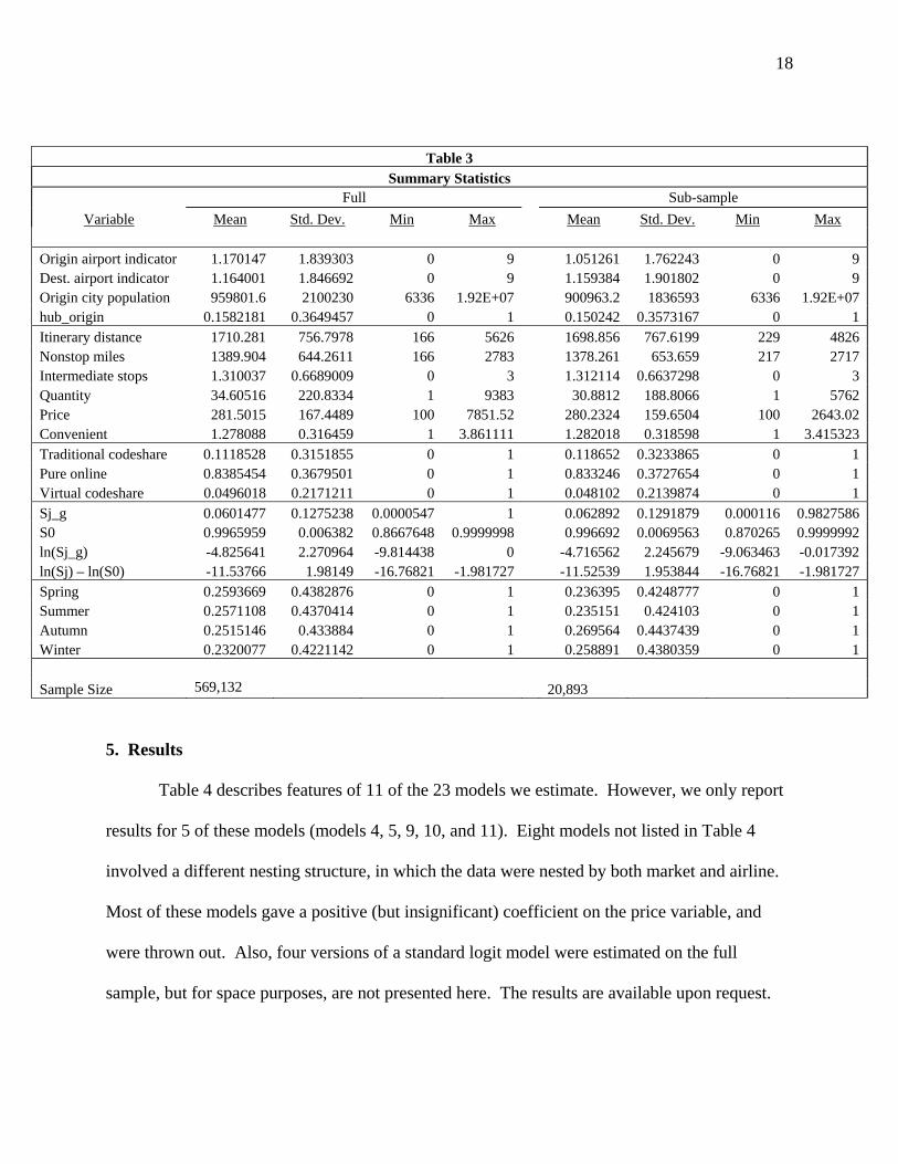
in almost half of the markets where either firm offers products. Summary statistics of the

samples used for estimation are presented in Table 3.

Table 2 Dual Presence of Delta and Northwest in Markets

Markets Quarter Total With DL With NW With Both 2007:2 56514 28131 22766 12549 2007:3 57314 28810 22329 12425 2007:4 56024 27566 22416 12293 2008:1 53228 25994 21591 11840

18

Table 3 Summary Statistics

Full Sub-sample Variable Mean Std. Dev. Min Max Mean Std. Dev. Min Max

Origin airport indicator 1.170147 1.839303 0 9 1.051261 1.762243 0 9 Dest. airport indicator 1.164001 1.846692 0 9 1.159384 1.901802 0 9 Origin city population 959801.6 2100230 6336 1.92E+07 900963.2 1836593 6336 1.92E+07 hub_origin 0.1582181 0.3649457 0 1 0.150242 0.3573167 0 1 Itinerary distance 1710.281 756.7978 166 5626 1698.856 767.6199 229 4826 Nonstop miles 1389.904 644.2611 166 2783 1378.261 653.659 217 2717 Intermediate stops 1.310037 0.6689009 0 3 1.312114 0.6637298 0 3 Quantity 34.60516 220.8334 1 9383 30.8812 188.8066 1 5762 Price 281.5015 167.4489 100 7851.52 280.2324 159.6504 100 2643.02 Convenient 1.278088 0.316459 1 3.861111 1.282018 0.318598 1 3.415323 Traditional codeshare 0.1118528 0.3151855 0 1 0.118652 0.3233865 0 1 Pure online 0.8385454 0.3679501 0 1 0.833246 0.3727654 0 1 Virtual codeshare 0.0496018 0.2171211 0 1 0.048102 0.2139874 0 1 Sj_g 0.0601477 0.1275238 0.0000547 1 0.062892 0.1291879 0.000116 0.9827586 S0 0.9965959 0.006382 0.8667648 0.9999998 0.996692 0.0069563 0.870265 0.9999992 ln(Sj_g) -4.825641 2.270964 -9.814438 0 -4.716562 2.245679 -9.063463 -0.017392 ln(Sj) – ln(S0) -11.53766 1.98149 -16.76821 -1.981727 -11.52539 1.953844 -16.76821 -1.981727 Spring 0.2593669 0.4382876 0 1 0.236395 0.4248777 0 1 Summer 0.2571108 0.4370414 0 1 0.235151 0.424103 0 1 Autumn 0.2515146 0.433884 0 1 0.269564 0.4437439 0 1 Winter 0.2320077 0.4221142 0 1 0.258891 0.4380359 0 1 Sample Size 569,132 20,893

5. Results

Table 4 describes features of 11 of the 23 models we estimate. However, we only report

results for 5 of these models (models 4, 5, 9, 10, and 11). Eight models not listed in Table 4

involved a different nesting structure, in which the data were nested by both market and airline.

Most of these models gave a positive (but insignificant) coefficient on the price variable, and

were thrown out. Also, four versions of a standard logit model were estimated on the full

sample, but for space purposes, are not presented here. The results are available upon request.

19

Table 4 List of regressions

Model Number Sample Estimation Technique Hub x Interstop Airline Dummies

1 Full 2SLS No No 2 Full 2SLS No Yes 3 Full 2SLS Yes No 4 Full 2SLS Yes Yes 5 Full OLS Yes Yes 6 Reduced 2SLS No No 7 Reduced 2SLS No Yes 8 Reduced 2SLS Yes No 9 Reduced OLS Yes Yes

10 Reduced 2SLS Yes Yes 11 Reduced GMM Yes Yes

For both the full sample and reduced sample, a nested logit was estimated with different

inclusions and exclusions of the hub_interstop variable and the airline dummies. These models

are estimated using 2SLS detailed below. The other model is the full specification on the

subsample using GMM estimation. An OLS model including airline dummies and the

hub_interstop variable is also estimated for comparison purposes. The full sample results of the

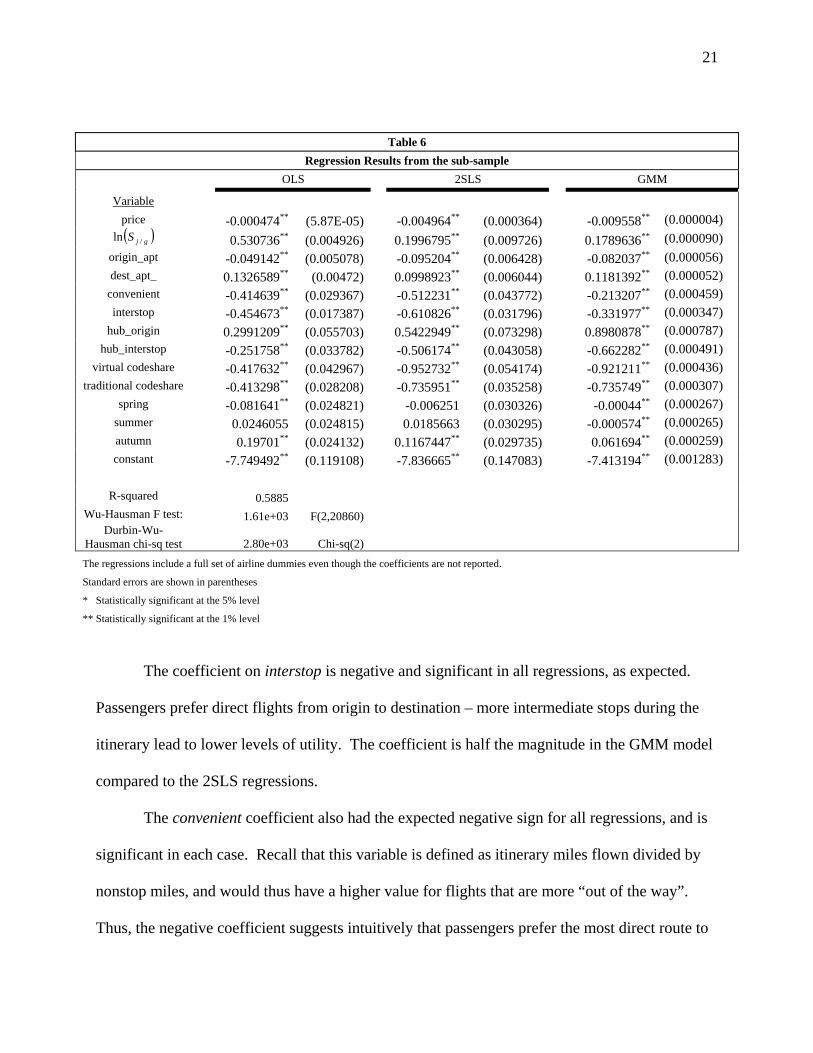
regressions are shown in Table 5, and the results of the subsample regressions including the

constrained GMM are shown in Table 6.

Variable signs and significance

To test the validity of the instruments, we regressed both endogenous variables against

the instruments using OLS and also performed a Hausman test. The results show that each

instrument is strongly correlated with the endogenous variables. These results are shown in

Appendix A. Hausman tests in Tables 5 and 6 also reject the exogeneity of price and ( )gjS /ln ,

implying that instruments are needed.18

18 The Hausman test presents a null hypothesis of price and ( )gjS /ln being exogenous. The Durbin-Wu-Hausman chi-square test with two degrees of freedom rejects the null hypothesis with over 99.99% confidence.

20

Table 5 Regression Results from the Full Sample

OLS 2SLS

Variable price -0.000337** (0.0000106) -0.003633** (6.37E-05) ( )gjS /ln 0.5638265** (0.0009369) 0.2346224** (0.001865)

origin_apt -0.016191** (0.0009283) -0.063835** (0.001123) dest_apt 0.1384643** (0.0009252) 0.0867591** (0.001129)

convenient -0.411686** (0.0056451) -0.567484** (0.008092) interstop -0.415735** (0.003287) -0.655274** (0.005567)

hub_origin 0.2285709** (0.0104666) 0.3411788** (0.012931) hub_interstop -0.2098** (0.0063686) -0.417027** (0.007655)

virtual codeshare -0.361678** (0.0080486) -0.872166** (0.009719) traditional codeshare -0.415568** (0.0054974) -0.704275** (0.006565)

spring 0.1070519** (0.0047444) 0.0732034** (0.005546) summer 0.0859185** (0.0047508) 0.0634193** (0.005552) autumn 0.0578049** (0.0047718) -0.001777** (0.005628) constant -7.747866** (0.0212766) -7.895797** (0.0252827)

R-squared 0.6023

Wu-Hausman F test: 3.68e+04 F(2,569099) Durbin-Wu-Hausman

chi-sq test 6.51e+04 Chi-sq(2) The regressions include a full set of airline dummies even though the coefficients are not reported.

Standard errors are shown in parentheses

* Statistically significant at the 5% level

** Statistically significant at the 1% level As expected, the coefficient on price is negative, implying that higher prices are

associated with lower levels of utility, ceteris paribus. Note that the magnitude of the coefficient

is much greater in the 2SLS and GMM regressions compared to OLS. Without the use of

instruments, OLS gives an underestimate of passengers’ disutility to higher prices. While there

is not a significant difference in the price coefficient between the full sample and sub-sample

with the 2SLS models, the GMM model estimates the price coefficient to be twice as large. The

larger coefficient implies an even greater underestimation of consumer price sensitivity with

OLS. Clearly, instruments for price are needed, and constraining the model to allow only

positive marginal costs has a large effect on the price coefficient as well.

21

Table 6 Regression Results from the sub-sample

OLS 2SLS GMM

Variable price -0.000474** (5.87E-05) -0.004964** (0.000364) -0.009558** (0.000004) ( )gjS /ln 0.530736** (0.004926) 0.1996795** (0.009726) 0.1789636** (0.000090)

origin_apt -0.049142** (0.005078) -0.095204** (0.006428) -0.082037** (0.000056) dest_apt_ 0.1326589** (0.00472) 0.0998923** (0.006044) 0.1181392** (0.000052)

convenient -0.414639** (0.029367) -0.512231** (0.043772) -0.213207** (0.000459) interstop -0.454673** (0.017387) -0.610826** (0.031796) -0.331977** (0.000347)

hub_origin 0.2991209** (0.055703) 0.5422949** (0.073298) 0.8980878** (0.000787) hub_interstop -0.251758** (0.033782) -0.506174** (0.043058) -0.662282** (0.000491)

virtual codeshare -0.417632** (0.042967) -0.952732** (0.054174) -0.921211** (0.000436) traditional codeshare -0.413298** (0.028208) -0.735951** (0.035258) -0.735749** (0.000307)

spring -0.081641** (0.024821) -0.006251 (0.030326) -0.00044** (0.000267) summer 0.0246055 (0.024815) 0.0185663 (0.030295) -0.000574** (0.000265) autumn 0.19701** (0.024132) 0.1167447** (0.029735) 0.061694** (0.000259) constant -7.749492** (0.119108) -7.836665** (0.147083) -7.413194** (0.001283)

R-squared 0.5885

Wu-Hausman F test: 1.61e+03 F(2,20860) Durbin-Wu-

Hausman chi-sq test 2.80e+03 Chi-sq(2)

The regressions include a full set of airline dummies even though the coefficients are not reported.

Standard errors are shown in parentheses

* Statistically significant at the 5% level

** Statistically significant at the 1% level

The coefficient on interstop is negative and significant in all regressions, as expected.

Passengers prefer direct flights from origin to destination – more intermediate stops during the

itinerary lead to lower levels of utility. The coefficient is half the magnitude in the GMM model

compared to the 2SLS regressions.

The convenient coefficient also had the expected negative sign for all regressions, and is

significant in each case. Recall that this variable is defined as itinerary miles flown divided by

nonstop miles, and would thus have a higher value for flights that are more “out of the way”.

Thus, the negative coefficient suggests intuitively that passengers prefer the most direct route to

22

the destination. While the sign is the same across all specifications, the magnitude is much

smaller in the GMM model.

In all regressions where the interaction term hub_interstop is not included, the coefficient

on hub_origin is negative, which was not the expected sign.19 However, the coefficient on

hub_origin turns positive (and significant) when the interaction term is added to the regression,

and the interaction term itself has a significantly negative coefficient. For a given market, a hub

airline and a non-hub airline could offer a product with the same number of intermediate stops.

The positive sign on hub_origin indicates a preference toward the hub product in this case.

However, if the hub product has a sufficiently larger number of intermediate stops compared to

the non-hub product, then the negative sign on hub_interstop suggests that the non-hub product

may be chosen over the hub product.

The negative coefficient on the origin airport indicator variable suggests that any given

product becomes more substitutable as the number of airports in the city increases. This is due to

increased levels of competition – a greater variety of products may draw customers away from

any given product.

The positive coefficient on the destination airport indicator illustrates higher demand for

itineraries with a destination city containing multiple airports. This may just be reflecting

unobserved factors – a larger city with more airports is more likely to also have increased tourist

or business activities, which would make airline travel to this destination more desirable.

The traditional variable has a negative and significant coefficient – note that the “left

out” product type category is pure online, so this indicates that a traditional codeshare product

has a lower demand relative to a pure online product. While there are multiple operating carriers

on this type of itinerary, the double markup may be eliminated because of a single ticketing 19 These regressions are not presented here.

23

carrier. Thus, the negative sign may be capturing some other unobserved handiness effects. The

flight itinerary for a pure online product is very streamlined, and a company can better organize

its own planes and schedules to minimize layover time, and efficiently organize gates at airports.

With a traditional codeshare flight, a passenger may be more likely to experience longer layovers

or longer journeys through the airport to find a different gate. Even though codeshare partners

try to coordinate their efforts in this manner, the negative coefficient on traditional codeshare

suggests that these coordination efforts are not perfect.

The coefficient on virtual is negative and significant in all regressions. Moreover, it is

greater in magnitude than the coefficient on traditional with the exception of the full sample

OLS. As previously noted in Ito and Lee (2007), this negative coefficient could be due to the

fact that virtual codeshare itineraries are a relatively inferior product – frequent flyer miles may

often not be used, and first-class upgrades are usually unavailable on this type of itinerary.

The significance of the season dummies (and sign in one case) depends on the model

specification. The summer dummy is always positive, and is significant in the full sample

regressions. The autumn dummy is positive and significant in all regressions. Summer travel

may be desirable for vacations, and autumn travel (which includes October – December) may be

desirable to visit family and friends over the holidays.

The coefficient on ( )gjS /ln is our estimate forσ . Note that this term only appears in the

nested logit specifications of the model, as the standard logit model does not use any nesting

methods to group products. The estimate forσ was as high as 0.564 in specification 5, and as

low as 0.179 in specification 11. The large variation in estimates once again illustrates the

importance of using instruments for endogenous variables. All estimates of σ are between 0 and

1 with significance, so the model is consistent with utility maximization.

24

Inference from Demand Elasticities

To get a sense of the substitutability between competing airlines’ products, it is

worthwhile to examine demand elasticities of the products. For comparison, we have selected

eight markets to study that differ by origin-destination distance and number of competing firms.

We compute a matrix of product elasticities for each market, where the main diagonal elements

are own-price elasticities, and the off-diagonal elements are cross-price elasticities. For each

market, the matrix will be of dimension ( ) JJ ×+1 , where J is the number of products in the

relevant market. The extra row in the matrix contains elasticity estimates for the outside good,

which includes transportation options that are not explicitly included in the model, such as

purchasing an airline product with multiple ticketing carriers, choosing non-airline

transportation, or not traveling at all.

However, we are most interested in competition at the firm/airline level rather than the

product level, so these product elasticities have been averaged according to product ownership

by airlines. Thus, for the elasticity matrices we present in Tables 7 and 8, an element is

interpreted as the average percent by which the row airline’s demand changes as the result of a 1

percent increase in the column airline’s product price.

As expected, the own price elasticities are negative and all of the cross-price elasticities

are positive, suggesting the airlines’ products are gross substitutes. Further, recall that for our

nested logit model, each market is defined as a nest. Thus, we see that the cross-price elasticities

are identical throughout any column in the matrix.

Consider the elasticities of the Boston-Los Angeles market, shown in Table 7. When

Delta raises its prices by 1%, the demand for Delta products in this market will decrease by

25

3.57%, and the demand for all other inside products20 will increase by 0.0047%. When

Northwest raises its prices by 1%, the demand for Northwest products in this market will fall by

4.43%, and the demand for other inside products will increase by 0.00210%. The cross-price

elasticity of the outside good ranges from 0.00001% for Alaska Airlines, to 0.00009% for

Midwest Express.21 In the Buffalo-Columbus market, shown in Table 8, the outside good has

estimated demand increases ranging from 0.00004% to 0.00014%. The higher elasticities of the

outside good for the Buffalo-Columbus market may be largely due to the shorter distance

between origin and destination, which implies that transportation alternatives such as driving are

more practical substitutes for air travel.

While demand elasticities are useful and easy to interpret, they do not give us a full

picture of the nature of the competition between the products within the market. To get a better

idea of competition, we pay particular attention to the fact that sales will decrease for a good that

experiences a price increase. Following Gayle (2007a), we want to see how those lost sales are

captured by competing products. To infer information about the transfer of lost sales in the event

of a price increase, we weight the elasticities by their respective quantities and divide the

weighted cross-price elasticity by its quantity weighted own-price elasticity. The resulting ratio

tells us the proportion of lost sales that are captured by a competitor or the outside good.

20 We refer to products that are included in the model as “inside” products. 21 To understand why the outside good elasticities are relatively small, we must consider that product shares are determined by the population of the origin city. Therefore, the share (outside good share) of the population that did not choose airline products that are included in our model is relatively large compared to shares for inside products. This implies that if similar amounts of people switch to the outside good as do to the inside goods, the percent change in the share of the outside good will be smaller than the percent change in the shares of inside goods.

26

Table 7 Price Elasticity of Demand Matrix (%)

Boston – Los Angeles, Nonstop flight miles = 2,611 DL NW CO AA AS FL UA US YX

DL -3.57287 0.00210 0.00183 0.00208 0.00158 0.00680 0.00239 0.00340 0.01002

NW 0.00470 -4.43044 0.00183 0.00208 0.00158 0.00680 0.00239 0.00340 0.01002

CO 0.00470 0.00210 -4.67455 0.00208 0.00158 0.00680 0.00239 0.00340 0.01002

AA 0.00470 0.00210 0.00183 -4.50683 0.00158 0.00680 0.00239 0.00340 0.01002

AS 0.00470 0.00210 0.00183 0.00208 -4.22108 0.00680 0.00239 0.00340 0.01002

FL 0.00470 0.00210 0.00183 0.00208 0.00158 -2.35082 0.00239 0.00340 0.01002

UA 0.00470 0.00210 0.00183 0.00208 0.00158 0.00680 -4.50823 0.00340 0.01002

US 0.00470 0.00210 0.00183 0.00208 0.00158 0.00680 0.00239 -4.94763 0.01002

YX 0.00470 0.00210 0.00183 0.00208 0.00158 0.00680 0.00239 0.00340 -2.08213

Outside 0.00004 0.00002 0.00002 0.00002 0.00001 0.00006 0.00002 0.00003 0.00009

Table 8 Price Elasticity of Demand Matrix (%)

Buffalo – Columbus, Nonstop flight miles = 296 DL NW CO UA US WN DL -1.46916 0.01510 0.03136 0.03317 0.03972 0.02965NW 0.05719 -2.84334 0.03136 0.03317 0.03972 0.02965CO 0.05719 0.01510 -1.97904 0.03317 0.03972 0.02965UA 0.05719 0.01510 0.03136 -1.92702 0.03972 0.02965US 0.05719 0.01510 0.03136 0.03317 -1.53040 0.02965WN 0.05719 0.01510 0.03136 0.03317 0.03972 -1.54782Outside 0.00014 0.00004 0.00007 0.00008 0.00009 0.00007

For example, consider three competitors, A, B, and C. Suppose the elasticities are

defined as A

A

A

AAA Q

PPQ∂∂

=η , A

B

B

ABA Q

PPQ∂∂

=η and A

C

C

ACA Q

PPQ∂∂

=η . The proportion of lost sales

captured by firm B in the event of a price increase of firm A’s product is given byAAA

BAB

QQ

ηη

×× ,

while the proportion of firm A’s lost sales captured by firm C is AAA

CAC

QQ

ηη

××

. If

AAA

CAC

AAA

BAB

QQ

QQ

ηη

ηη

××

>×× , we can conclude that airline B is a closer competitor to airline A than

airline C is to airline A.

27

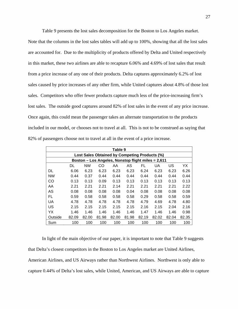
Table 9 presents the lost sales decomposition for the Boston to Los Angeles market.

Note that the columns in the lost sales tables will add up to 100%, showing that all the lost sales

are accounted for. Due to the multiplicity of products offered by Delta and United respectively

in this market, these two airlines are able to recapture 6.06% and 4.69% of lost sales that result

from a price increase of any one of their products. Delta captures approximately 6.2% of lost

sales caused by price increases of any other firm, while United captures about 4.8% of those lost

sales. Competitors who offer fewer products capture much less of the price-increasing firm’s

lost sales. The outside good captures around 82% of lost sales in the event of any price increase.

Once again, this could mean the passenger takes an alternate transportation to the products

included in our model, or chooses not to travel at all. This is not to be construed as saying that

82% of passengers choose not to travel at all in the event of a price increase.

Table 9 Lost Sales Obtained by Competing Products (%)

Boston – Los Angeles, Nonstop flight miles = 2,611 DL NW CO AA AS FL UA US YX DL 6.06 6.23 6.23 6.23 6.23 6.24 6.23 6.23 6.26 NW 0.44 0.37 0.44 0.44 0.44 0.44 0.44 0.44 0.44 CO 0.13 0.13 0.09 0.13 0.13 0.13 0.13 0.13 0.13 AA 2.21 2.21 2.21 2.14 2.21 2.21 2.21 2.21 2.22 AS 0.08 0.08 0.08 0.08 0.04 0.08 0.08 0.08 0.08 FL 0.59 0.58 0.58 0.58 0.58 0.29 0.58 0.58 0.59 UA 4.78 4.78 4.78 4.78 4.78 4.79 4.69 4.78 4.80 US 2.15 2.15 2.15 2.15 2.15 2.16 2.15 2.04 2.16 YX 1.46 1.46 1.46 1.46 1.46 1.47 1.46 1.46 0.98 Outside 82.09 82.00 81.98 82.00 81.98 82.19 82.02 82.04 82.35 Sum 100 100 100 100 100 100 100 100 100

In light of the main objective of our paper, it is important to note that Table 9 suggests

that Delta’s closest competitors in the Boston to Los Angeles market are United Airlines,

American Airlines, and US Airways rather than Northwest Airlines. Northwest is only able to

capture 0.44% of Delta’s lost sales, while United, American, and US Airways are able to capture

28

4.78%, 2.21%, and 2.15% respectively. However, Delta is Northwest’s closest competitor

followed by United, American, and US Airways respectively. This information is useful since

the weaker the pre-merger degree of competitiveness between firms that subsequently merger,

the smaller is the price increase that will result from the merger, ceteris paribus.

The lost sales matrix for the Buffalo – Columbus market, a competitive shorter-distance

market, is displayed in Table 10. The X entries along the diagonal mean that a firm only offers

one product in the market and cannot recapture lost sales through other products. In this

particular market, US Airways appears to be the dominant firm, capturing approximately 5.5% to

5.6% of other competitors’ sales in the event of a price increase. Delta and United each capture

approximately 3.8% of competitors’ lost sales. It is also important to note that Delta and

Northwest seem not to be strong competitors for each other in the Buffalo – Columbus market.

In the Buffalo – Columbus market, the outside good captures a slightly larger portion of

lost sales compared to the long-distance Boston – Los Angeles market. This is largely due to

alternative transportation being more viable for short distances. However, in both cases, the

portion of lost sales captured by the outside good is relatively high (over 80%).22

Table 10 Lost Sales Obtained by Competing Products (%) Buffalo – Columbus, Nonstop flight miles = 296

DL NW CO UA US WN DL X 3.77 3.81 3.82 3.85 3.82 NW 1.73 1.11 1.69 1.69 1.71 1.69 CO 1.62 1.57 X 1.59 1.60 1.59 UA 3.82 3.70 3.74 1.87 3.78 3.75 US 5.62 5.44 5.49 5.51 2.77 5.51 WN 1.95 1.89 1.91 1.91 1.93 X Outside 85.26 82.52 83.36 83.61 84.35 83.63 Sum 100 100 100 100 100 100

22 Gayle (2007a) found estimates of the outside good capturing larger amounts of lost sales, often more than 95%. In his paper, traditional codeshare products are considered to be part of the outside good. Since our model includes traditional codeshare products as part of the inside good, our outside good encompasses a smaller number of alternatives, and it is clear to see why the outside good in our paper will capture a smaller amount of lost sales caused by a price increase of any given airline product.

29

The tables describing elasticities and lost sales for six other markets are shown in

Appendix B. In general, we find that Delta and Northwest are not always the strongest

competitors for each other, but even when they are, the outside good seems to be a sufficiently

attractive alternative to constrain the joint pricing behavior of the two airlines. This seems to be

especially true for shorter-distance markets.

Merger Analysis

Since our main objective is to analyze the merger, recall that our dataset includes only

markets that contain both Delta and Northwest products before the merger.23 This will allow us

to isolate the merger effects in markets where the two firms’ services overlap. Summary

statistics for variables of interest in the subsample are displayed in Table 11. The average pre-

merger markup is approximately $89.78. The average predicted change in price is only an

increase of 0.54%, hardly big enough to concern consumers, let alone antitrust authorities.

However, the maximum predicted increase in price is over 13%.

Table 11 Summary statistics of merger analysis

Variable Mean Std. Dev. Min Max Pre-merger marginal costs 190.4556 159.75 5.02E-07 2556.969 Pre-merger markup 89.7768 2.918 85.90399 104.5631 Post-merger predicted price 281.4915 159.66 100.0047 2643.021 Predicted Price Increases (percent) 0.543886 1.0818 0 13.0983 Delta/Northwest pre-merger combined market passenger share 35.75316 27.34 0.578927 100

To get a more detailed analysis of Delta/Northwest dominance in different markets, we

calculated the combined passenger share that Delta and Northwest had in each market. For

example, if 1,000 passengers flew from Minneapolis to Atlanta and 400 of them flew on Delta or

Northwest tickets, then the Delta/Northwest share for this market is 40%. Note that this share is

23 Markets that include neither firm or just one of the two firms will not experience a price increase according to our model since the ownership structure of products will be the same before and after the merger.

30

calculated by passengers, and not by the number of flights. This is displayed in the last row in

Table 11. On average, Delta and Northwest own over one-third (35.75%) of the passenger share

in markets where both firms competed before the merger.

Summary statistics suggest a positive relationship between pre-merger Delta/Northwest

combined market passenger share and predicted price increases. As shown in Table 11, all

products and markets considered, the average predicted percent increase in price is 0.54% and

the average pre-merger Delta/Northwest combined passenger share in markets is 35.75%.

However, for products with a predicted price increase between 1% and 3%, the average

Delta/Northwest combined passenger share in the market is 48.76%, and for predicted price

increases of 3% or more, the average Delta/Northwest combined passenger share in the market is

65.19%. For markets where Delta and Northwest have a 100% combined passenger share,

average predicted price increase is 3.47%. While a 3.47% predicted price increase seems small

for a market that would become a post-merger monopoly, we must remember that the outside

good option may help keep airline prices low. Interestingly, the potential post-merger monopoly

markets tended to be short-distance markets in which the outside good has a greater effect on

demand for airline products. 24

To rigorously examine the association between Delta/Northwest pre-merger combined

passenger share and predicted price increases, we regress the predicted percent change in prices

as a function of the Delta/Northwest combine passenger share (quantshareDN) as well as some

other control variables. We also use the same approach to examine the association between

24 Since our merger analysis is only considering markets where Delta and Northwest both offer products before the merger, a 100% Delta/Northwest combined share means that there was a pre-merger duopoly. After the merger, the market becomes a monopoly, thus explaining the larger predicted price increase. This occurred in 72 markets, but most markets had only small quantities of passengers. Larger quantity markets in which this occurred include nonstop service between Detroit and Cincinnati and nonstop service between Cincinnati and Nashville, both short-distance markets.

31

Delta/Northwest pre-merger combined passenger share and markups. The estimates are

displayed in Table 12.

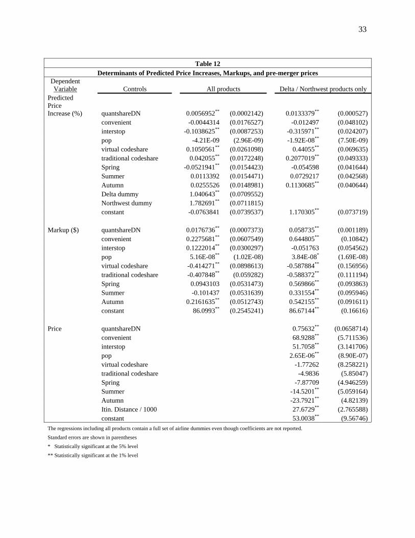
These results allow us to see what factors determine the predicted post-merger price

increases. The regressions show that prices are predicted to increase by larger amounts the larger

is Delta/Northwest combine pre-merger passenger share in a market. However, while these

results are statistically significant, they are not economically significant. For instance, among all

products, a 1% increase in the pre-merger share of Delta/Northwest passengers in a market

would increase markups by 2 cents, and would cause prices to increase by 0.0056 percent.

Considering Delta/Northwest products only, markups will increase by 6 cents, and price would

increase by 0.013 percent. The negative coefficients on convenient and interstop suggest that

prices are predicted to increase less for less convenient and intermediate stop(s) itineraries.

The left panel of the table also included dummy variables for all the airlines, but these

estimates are not reported with the exception of the Delta and Northwest dummies for the price

increase regression. It is worth noting that being a Delta or Northwest product has a much larger

influence on the predicted price increase than any of the other control variables.

We next ran the same regression using just the Delta and Northwest products, and the

results are shown in the right panel of Table 12. The sign and significance of all the variables

remain the same, and the coefficients on the codeshare variables and the quantity share variable

increase in magnitude.

Although the predicted price increases are relatively small, it is worthwhile to examine

their distribution among product owners. While the mean percent price change is 1.45% for

Delta/Northwest products, the entire sample had many larger price increases. 3,942 of the

20,893 products experienced price increases larger than 1%, all of which were Delta/Northwest

32

products. Of these, 929 products had price increases greater than 3%, and 201 products had

price increases greater than 5%. Figure 1 shows the distribution of predicted price increases

among Delta/Northwest and other products.

Figure 1 shows that non-Delta/Northwest products’ predicted price increases are smaller

than 1 percent, and are in fact less than a quarter of a percent. Again, most predicted price

increases are very small, but the smallest increases are limited mostly to the non-Delta/Northwest

products. The largest estimated price increase for a non-Delta/Northwest product was just 0.2

percent. Products that are experiencing larger predicted price increases are exclusively

Delta/Northwest products. Furthermore, in terms of pre-merger price levels, itinerary distance,

and convenience, these Delta/Northwest products with relatively large predicted price increases

are not significantly different from products in the entire sample.

For predicted price increases on the Delta/Northwest products, the coefficients on

traditional codeshare and virtual codeshare in Table 12 are significantly positive, implying that

these types of products will experience higher price increases (in terms of percentages) relative

to pure online products. However, the results indicate that these two product types have lower

absolute markups, although the difference is trivial. To examine this further, we regressed the

pre-merger price against market and product characteristics and found negative but statistically

insignificant coefficients on virtual codeshare and traditional codeshare variables. Thus, the

price regression in the bottom panel of Table 12 suggests that, on average, Delta and Northwest

codeshare products are priced similar to their pure online products in the pre-merger period, but

the predicted price increase regression in the top right panel of Table 12 suggests that Delta and

Northwest codeshare products’ prices will increase by more than their prices for pure online

products.

33

Table 12

Determinants of Predicted Price Increases, Markups, and pre-merger prices Dependent Variable

Controls

All products Delta / Northwest products only

Predicted Price Increase (%)

quantshareDN

0.0056952** (0.0002142) 0.0133379** (0.000527) convenient -0.0044314 (0.0176527) -0.012497 (0.048102) interstop -0.1038625** (0.0087253) -0.315971** (0.024207) pop -4.21E-09 (2.96E-09) -1.92E-08** (7.50E-09) virtual codeshare 0.1050561** (0.0261098) 0.44055** (0.069635) traditional codeshare 0.042055** (0.0172248) 0.2077019** (0.049333) Spring -0.0521941** (0.0154423) -0.054598 (0.041644) Summer 0.0113392 (0.0154471) 0.0729217 (0.042568) Autumn 0.0255526 (0.0148981) 0.1130685** (0.040644) Delta dummy 1.040643** (0.0709552) Northwest dummy 1.782691** (0.0711815) constant -0.0763841 (0.0739537) 1.170305** (0.073719) Markup ($) quantshareDN 0.0176736** (0.0007373) 0.058735** (0.001189) convenient 0.2275681** (0.0607549) 0.644805** (0.10842) interstop 0.1222014** (0.0300297) -0.051763 (0.054562) pop 5.16E-08** (1.02E-08) 3.84E-08* (1.69E-08) virtual codeshare -0.414271** (0.0898613) -0.587884** (0.156956) traditional codeshare -0.407848** (0.059282) -0.588372** (0.111194) Spring 0.0943103 (0.0531473) 0.569866** (0.093863) Summer -0.101437 (0.0531639) 0.331554** (0.095946) Autumn 0.2161635** (0.0512743) 0.542155** (0.091611) constant 86.0993** (0.2545241) 86.67144** (0.16616) Price quantshareDN 0.75632** (0.0658714) convenient 68.9288** (5.711536) interstop 51.7058** (3.141706) pop 2.65E-06** (8.90E-07) virtual codeshare -1.77262 (8.258221) traditional codeshare -4.9836 (5.85047) Spring -7.87709 (4.946259) Summer -14.5201** (5.059164) Autumn -23.7921** (4.82139) Itin. Distance / 1000 27.6729** (2.765588) constant 53.0038** (9.56746) The regressions including all products contain a full set of airline dummies even though coefficients are not reported.

Standard errors are shown in parentheses

* Statistically significant at the 5% level

** Statistically significant at the 1% level

34

Figure 1Predicted Price Increase Distribution

across Product Ownership

0

2000

4000

6000

8000

10000

12000

14000

0 - 0.25 0.25 - 1.0 1.0 - 3.0 3.0 and upPercent Price Increase Categories

Num

ber

of P

rodu

cts

All other productsDelta / Northwest

Figure 2 shows the predicted price increases among Delta/Northwest products distributed

among different types of products. It is clear from Figure 2 that the number of pure online

products is greater than the number of traditional codeshare and virtual codeshare products in all

predicted price increase categories.

Although the regressions in Table 12 suggest that both types of codeshare products on

average have higher predicted price increases compared to pure online products, in Figure 2 it

appears that there is a relatively similar distribution of price increases among all types of

products. To see the distribution pattern a little more clearly, we created a 100% stacked column

chart in Figure 3 to show the percent of each product type in each price increase range. Figure 3

reveals that codeshare products make up a higher ratio of the highest price increases compared to

the lowest price increases and conversely for pure online products.

35

Figure 2Predicted Price Increase Distribution across Product Types

for Delta/Northwest Products

0

500

1000

1500

2000

2500

3000

3500

0 - 1.0 1.0 - 3.0 3.0 - 6.0 6.0 and upPercent Price Increase Categories

Num

ber

of P

rodu

cts Pure Online

Traditional CodeshareVirtual Codeshare

Figure 3Predicted Price Increase Distribution acrossProduct Types for Delta/Northwest Products

0%

20%

40%

60%

80%

100%

0 - 1.0 1.0 - 3.0 3.0 - 6.0 6.0 - 9.0 9.0 and upPercent Price Increase Categories

Perc

ent o

f Pro

duct

s

Virtual CodeshareTraditional CodesharePure Online

36

Figures 2 and 3 use only information about product types before the merger. However,

products may change type classification after Delta and Northwest merge because the ownership

structure of the products changes. Specifically, one of five things could happen to

Delta/Northwest’s products after the merger:

1. A pure online product remains a pure online product (6593 products)

2. A traditional codeshare product remains a traditional codeshare product (327 products)

3. A traditional codeshare product becomes a pure online product (444 products)

4. A virtual codeshare product remains a virtual codeshare product (73 products)

5. A virtual codeshare product becomes a pure online product (302 products)

For ease of analysis, we sort these products into 5 groups according to the number of

cases above. For example, group 3 is the group of products that were of type traditional

codeshare before the merger and will become pure online products after the simulated merger.

One reason why product groups 2 – 5 arise is that Delta, Northwest, and Continental are

codeshare alliance partners prior to the Delta/Northwest merger. As such, many of Delta and

Northwest’s codeshare products involve Continental as an operating carrier, and therefore these

products keep their classification as codeshare products after our simulated Delta/Northwest

merger. However, the codeshare products that only involve Delta and Northwest as either

operating or ticketing carriers, will become pure online products with the simulated

Delta/Northwest merger.

It is of particular interest to see if these five scenarios differ in terms of predicted price

increases. We examine this in the left panel of Table 13, which includes only Delta/Northwest

products. Using OLS, we regress the predicted price increase against a set of dummy variables

that capture cases 2 – 5, as well as some previously used regressors. Note that the group

37

dummies in Table 13 are simply a decomposition of the traditional codeshare and virtual

codeshare dummies used in Table 12. On the right panel of Table 13, we change the dependent

variable to pre-merger price, and add itinerary distance as an additional regressor.

We observe some interesting effects for the groups. Note that group 1 is the excluded

category, which are products that were pure online before the merger. We see positive and

statistically significant coefficients on the Group 3 and Group 5 dummies, indicating that pre-

merger codeshare products which become pure online products after the simulated merger

experience higher predicted price increases. Specifically, products that were traditional

codeshare products experience an additional 0.36% predicted price increase when they become

pure online products, and the virtual codeshare products have an additional 0.58% predicted

price increase when they become pure online products. We see insignificant predicted price

increase differences between products that stay within their codeshare type after the simulated

merger (Groups 2 and 4) compared to pre-merger pure online products (Group 1).

Table 13 Determinants of Predicted Price Increases and Pre-merger Prices when

Delta/Northwest Codeshare Products are Decomposed into Groups Dependent Variable

Regressors Predicted Price Increase Pre-merger Price Group 2 0.0039158 (0.0730369) 11.37888 (8.67023) Group 3 0.3609901** (0.0634254) -17.33308* (7.529311) Group 4 -0.1910077 (0.1538667) 61.2043** (18.27282) Group 5 0.5859146** (0.0763692) -16.27636† (9.066044) quantshareDN 0.0132348** (0.0005267) 0.7666026** (0.065841) convenient -0.0140214 (0.0479987) 69.10002** (5.704503) interstop -0.327511** (0.0242688) 52.73332** (3.146785) pop -1.76E-08* (7.49E-09) 2.50E-06** (8.90E-07) spring -0.0577172 (0.0415705) -7.553413 (4.941739) summer 0.0654087 (0.0424962) -13.83555** (5.054985) autumn 0.1082129** (0.0405731) -23.28909** (4.817434) Itin. Distance / 1000 27.9077** (2.764374) constant 1.194922** (0.0736937) 50.31847** (9.577172) Standard errors are shown in parentheses † Statistically significant at the 10% level * Statistically significant at the 5% level ** Statistically significant at the 1% level

38

The right side of Table 13 shows a statistically significant negative coefficient on Group

3 and a marginally statistical significant negative coefficient on Group 5. These results suggest

that products in Groups 3 and 5 had lower pre-merger prices relative to pure online products.

This could explain why products in Groups 3 and 5 have larger predicted percent price increases.

Finally, we examine competition at the market level. To do this, dummy variables are

created to indicate the presence of competitors in the market. Next, we calculated the 25th

percentile, median, and 75th percentile of predicted price increases in each market so as to

capture what is happening at contrasting points of the predicted price increase distribution. The

predicted price increases are regressed against the Delta/Northwest combined passenger share,

competitors, and market characteristics including distance and population in three separate

regressions reported in Table 14. Each observation in these regressions represents a market

rather than a product.

As expected, the coefficient on Delta/Northwest combined passenger share is positive,

implying that Delta and Northwest product prices are predicted to increase by a greater amount

when their combined pre-merger passenger share in the market is larger. The origin city

population coefficient is negative and statistically significant, but the magnitude is too small to

draw any useful inferences. The origin airport indicator switches signs across the three

regressions, but is never significant. Interestingly, the destination airport indicator is negative,

implying lower price increases for markets with a destination that includes multiple airports.

This could reflect that multiple airports at the destination mean more substitute products are

available to help a passenger arrive at the destination, and more substitutes implies lower price

increases. The coefficients on Nonstop Miles are statistically insignificant.

39

Table 14 Percent Predicted Price Increases at Various Market Percentiles

Market Percentile Variable 25 50 75

DN Quantity share 0.0033843** (0.000329) 0.004247** (0.0004009) 0.0058518** (0.00056) Origin Population -1.45E-08** (4.01E-09) -1.79E-08** (4.88E-09) -3.07E-08** (6.82E-09) Origin Airport Ind -0.002577 (0.0049394) 0.0012675 (0.0060186) 0.005044 (0.008404) Dest Airport Ind -0.01881** (0.0048741) -0.016947** (0.005939) -0.008946 (0.008293) Nonstop Miles -1.46E-05 (0.0000158) -1.65E-05 (0.0000192) -3.02E-05 (2.68E-05)

American Airlines -0.139769** (0.0200172) -0.160925** (0.0243908) -0.416562** (0.034058) Alaskan Airlines -0.099836** (0.0278449) -0.140525** (0.0339289) -0.104442* (0.047376) JetBlue Airways -0.120099** (0.0278787) -0.189751** (0.03397) -0.275585** (0.047433)

Continental Airlines -0.162576** (0.0209823) -0.225551** (0.0255668) -0.259872** (0.0357) Frontier Airlines -0.19229** (0.0233945) -0.243447** (0.0285061) -0.391177** (0.039804) Airtran Airways -0.181877** (0.0196091) -0.217051** (0.0238936) -0.427313** (0.033363)

Allegiant Air -0.568166** (0.1042019) -0.783234** (0.1269694) -1.397824** (0.177291) America West -0.078514* (0.0380866) -0.11958** (0.0464084) -0.228961** (0.064801) Spirit Airlines -0.11466 (0.0610108) -0.138017 (0.0743413) -0.157658 (0.103805)

Skippers Aviation -0.398153** (0.058477) -0.552464** (0.071254) -0.788135** (0.099494) ATA Airlines 0.2160539** (0.0667692) 0.2175163** (0.0813579) 0.4975626** (0.113603)

International Business Air -0.319877** (0.0951806) -0.428963** (0.1159771) -0.77928** (0.161942) United Airlines -0.308193** (0.0227335) -0.386593** (0.0277006) -0.651063** (0.038679)

US Airways -0.344432** (0.0192305) -0.42636** (0.0234323) -0.462084** (0.032719) Southwest 0.1067443** (0.0209767) 0.0951628** (0.02556) 0.1027032** (0.03569) Midwest 0.2376883** (0.0245274) 0.2793229** (0.0298865) 0.2132134** (0.041732) constant 1.575415** (0.0372152) 2.035335** (0.0453465) 3.186354** (0.063319)

Standard errors are shown in parentheses

* Statistically significant at the 5% level

** Statistically significant at the 1% level

Most of the major airlines’ presence indicator variables have a negative coefficient, as

expected. The presence of other airlines offering competing products will keep the prices of

Delta/Northwest products lower. However, the coefficients on Southwest and Midwest are

positive. Interestingly, Southwest still has the largest mean passenger share even after

combining Delta and Northwest passenger shares.25 The positive coefficient for the presence of

25 This can be seen using just the 2008:1 dataset, which was the most recent available data. Without using our previously mentioned data filters, Southwest had a passenger share of 20.2%, while Delta and Northwest combined had a passenger share of 19.1%. These are very close to the results presented at the May 14th, 2008 hearing (see footnote 27) which illustrated that, using 2007:3 data, Southwest had a 19.4% passenger share and Delta/Northwest had a 19.2% passenger share.

40

Southwest variable may be suggesting that Southwest’s products are sufficiently differentiated

from Delta/Northwest products, thus limiting the amount of competition between the two.

Notwithstanding the positive coefficients on Southwest and Midwest, the overall message

to take away from Table 14 is that the presence of other airlines in a market matter for restraining

the exercise of market power. Furthermore, this result holds at contrasting points of the

predicted price increase distribution (25th, 50th, and 75th percentiles). As such, antitrust

authorities may want to pay closer attention to markets that may become a monopoly or duopoly

after the merger.26

6. Conclusions

Using a structural econometric model and pre-merger data, this paper studied the

potential effects of the imminent Delta/Northwest merger. Our findings suggest that, on average,

the Delta/Northwest merger will not cause significant price increases. We predict larger price

increases in markets that are dominated by Delta and Northwest, and on the Delta/Northwest

products themselves. However, even in markets that have a large pre-merger share of

Delta/Northwest products, the outside good option has the ability to restrain extremely large

price increases, particularly in short-distance markets. To prevent market power abuse in

concentrated markets, the DoJ may want to carefully monitor prices and behavior in markets that

have the largest combined Delta/Northwest passenger shares. Further, we find an interesting

result with positive price increases associated with the presence of Southwest. Once again, the

DoJ may want to monitor activity after the merger.

26 Such potential post-merger duopoly markets include non-stop service from Atlanta to Detroit, Memphis, and Minneapolis. However, Airtran, not Southwest, is the one large competitor to Delta and Northwest in these markets during the pre-merger period. In particular, Delta and Northwest have a 76.2% combined share in the Atlanta-Minneapolis non-stop market.

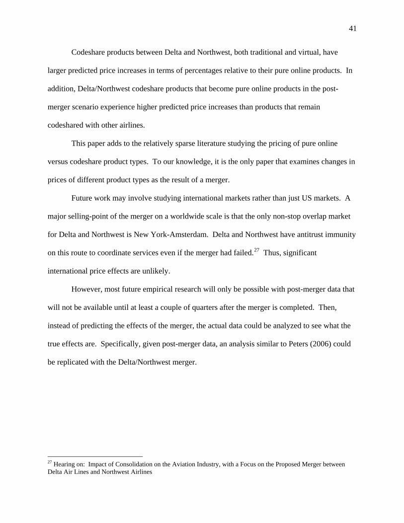
41

Codeshare products between Delta and Northwest, both traditional and virtual, have

larger predicted price increases in terms of percentages relative to their pure online products. In

addition, Delta/Northwest codeshare products that become pure online products in the post-

merger scenario experience higher predicted price increases than products that remain

codeshared with other airlines.

This paper adds to the relatively sparse literature studying the pricing of pure online

versus codeshare product types. To our knowledge, it is the only paper that examines changes in

prices of different product types as the result of a merger.

Future work may involve studying international markets rather than just US markets. A

major selling-point of the merger on a worldwide scale is that the only non-stop overlap market

for Delta and Northwest is New York-Amsterdam. Delta and Northwest have antitrust immunity

on this route to coordinate services even if the merger had failed.27 Thus, significant

international price effects are unlikely.

However, most future empirical research will only be possible with post-merger data that

will not be available until at least a couple of quarters after the merger is completed. Then,

instead of predicting the effects of the merger, the actual data could be analyzed to see what the

true effects are. Specifically, given post-merger data, an analysis similar to Peters (2006) could

be replicated with the Delta/Northwest merger.

27 Hearing on: Impact of Consolidation on the Aviation Industry, with a Focus on the Proposed Merger between Delta Air Lines and Northwest Airlines

42

Appendix A

Table A Instrument Validity Test

Dependent Variable Price ln(Sj_g)

Variable Nest_sum_convenient 1.463295** (0.0546008) -0.008004** (0.000586) Nest_sum_interstop 1.857765** (0.0400207) 0.072533** (0.0004295) Nest_convenient 93.69689** (2.098047) -2.679663** (0.0225185) Nest_interstop -56.56643** (1.551663) -1.014712** (0.0166541) N_comp -3.988629** (0.1054436) -0.154685** (0.0011317) N_multi -3.334339** (0.1071853) -0.145705** (0.0011504) comp_distance -0.266418** (0.0303568) 0.004013** (0.0003258) close_comp -3.275914** (0.0311703) 0.047139** (0.0003346) Itinerary distance / 1000 75.41188** (0.3987598) -0.679823** (0.0042799) constant 116.7935** (3.541902) 2.501058** (0.0380155)

R-squared 0.1216 0.4499 Standard errors are shown in parentheses

* Statistically significant at the 5% level

** Statistically significant at the 1% level

43

Appendix B

Table B1 Price Elasticity of Demand Matrices (%)

Post-Merger Monopoly Markets

Nashville – Cincinatti Nonstop Miles = 230

Detroit Metro – Cincinnati Nonstop Miles = 229

Pensacola – Sioux Falls Nonstop Miles = 1,045

Tennessee Tri-cities – San Antonio Nonstop Miles = 1,046

DL NW DL NW DL NW DL NW DL -4.35788 0.11682 -4.65038 0.19437 -4.37904 0.14772 -3.22370 0.18604 NW 0.09438 -1.41943 0.10170 -3.53221 0.21137 -3.99507 0.19336 -2.63880 Outside 0.00008 0.00009 0.00005 0.00010 0.00004 0.00004 0.00007 0.00007

Table B2

Price Elasticity of Demand Matrix (%) Dayton – Grand Rapids, Nonstop Miles = 217

DL NW CO AA UA YX DL -2.49763 0.10199 0.02012 0.08516 0.08586 0.05140NW 0.10768 -1.86379 0.02012 0.08516 0.08586 0.05140CO 0.10768 0.10199 -4.33055 0.08516 0.08586 0.05140AA 0.10768 0.10199 0.02012 -2.49319 0.08586 0.05140UA 0.10768 0.10199 0.02012 0.08516 -2.71380 0.05140YX 0.10768 0.10199 0.02012 0.08516 0.08586 -2.87335Outside 0.00009 0.00008 0.00002 0.00007 0.00007 0.00004

Table B3

Price Elasticity of Demand Matrix (%) Las Vegas – Atlanta, Nonstop Miles = 1,747

DL NW CO AA F9 FL UA US HP NK YX DL -4.45943 0.00283 0.00093 0.00278 0.00345 0.00461 0.00323 0.00201 0.00214 0.13411 0.00176 NW 0.00208 -2.20189 0.00093 0.00278 0.00345 0.00461 0.00323 0.00201 0.00214 0.13411 0.00176 CO 0.00208 0.00283 -5.02315 0.00278 0.00345 0.00461 0.00323 0.00201 0.00214 0.13411 0.00176 AA 0.00208 0.00283 0.00093 -3.42165 0.00345 0.00461 0.00323 0.00201 0.00214 0.13411 0.00176 F9 0.00208 0.00283 0.00093 0.00278 -2.90501 0.00461 0.00323 0.00201 0.00214 0.13411 0.00176 FL 0.00208 0.00283 0.00093 0.00278 0.00345 -2.45981 0.00323 0.00201 0.00214 0.13411 0.00176 UA 0.00208 0.00283 0.00093 0.00278 0.00345 0.00461 -2.82749 0.00201 0.00214 0.13411 0.00176 US 0.00208 0.00283 0.00093 0.00278 0.00345 0.00461 0.00323 -2.97188 0.00214 0.13411 0.00176 HP 0.00208 0.00283 0.00093 0.00278 0.00345 0.00461 0.00323 0.00201 -2.15765 0.13411 0.00176 NK 0.00208 0.00283 0.00093 0.00278 0.00345 0.00461 0.00323 0.00201 0.00214 -1.74551 0.00176 YX 0.00208 0.00283 0.00093 0.00278 0.00345 0.00461 0.00323 0.00201 0.00214 0.13411 -3.42672 Outside 0.00002 0.00003 0.00001 0.00003 0.00004 0.00005 0.00003 0.00002 0.00002 0.00137 0.00002

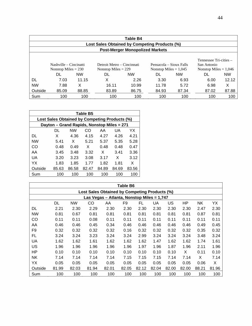
44

Table B4

Lost Sales Obtained by Competing Products (%) Post-Merger Monopolized Markets

Nashville – Cincinatti Nonstop Miles = 230

Detroit Metro – Cincinnati Nonstop Miles = 229

Pensacola – Sioux Falls Nonstop Miles = 1,045

Tennessee Tri-cities – San Antonio Nonstop Miles = 1,046

DL NW DL NW DL NW DL NW DL 7.03 11.15 X 2.26 3.30 6.93 6.00 12.12NW 7.88 X 16.11 10.99 11.78 5.72 6.98 X Outside 85.09 88.85 83.89 86.75 84.93 87.34 87.02 87.88Sum 100 100 100 100 100 100 100 100

Table B5 Lost Sales Obtained by Competing Products (%)

Dayton – Grand Rapids, Nonstop Miles = 271 DL NW CO AA UA YX DL X 4.36 4.15 4.27 4.26 4.21NW 5.41 X 5.21 5.37 5.35 5.28CO 0.48 0.49 X 0.48 0.48 0.47AA 3.45 3.48 3.32 X 3.41 3.36UA 3.20 3.23 3.08 3.17 X 3.12YX 1.83 1.85 1.77 1.82 1.81 X Outside 85.63 86.58 82.47 84.89 84.69 83.56Sum 100 100 100 100 100 100

Table B6

Lost Sales Obtained by Competing Products (%) Las Vegas – Atlanta, Nonstop Miles = 1,747

DL NW CO AA F9 FL UA US HP NK YX DL 2.21 2.30 2.29 2.30 2.30 2.30 2.30 2.30 2.30 2.47 2.30NW 0.81 0.67 0.81 0.81 0.81 0.81 0.81 0.81 0.81 0.87 0.81CO 0.11 0.11 0.08 0.11 0.11 0.11 0.11 0.11 0.11 0.11 0.11AA 0.46 0.46 0.45 0.34 0.46 0.46 0.46 0.46 0.46 0.49 0.45F9 0.32 0.32 0.32 0.32 0.16 0.32 0.32 0.32 0.32 0.35 0.32FL 3.24 3.24 3.23 3.24 3.24 2.99 3.24 3.24 3.24 3.48 3.24UA 1.62 1.62 1.61 1.62 1.62 1.62 1.47 1.62 1.62 1.74 1.61US 1.96 1.96 1.96 1.96 1.96 1.97 1.96 1.87 1.96 2.11 1.96HP 0.10 0.10 0.10 0.10 0.10 0.10 0.10 0.10 X 0.11 0.10NK 7.14 7.14 7.14 7.14 7.15 7.15 7.15 7.14 7.14 X 7.14YX 0.05 0.05 0.05 0.05 0.05 0.05 0.05 0.05 0.05 0.06 X Outside 81.99 82.03 81.94 82.01 82.05 82.12 82.04 82.00 82.00 88.21 81.96Sum 100 100 100 100 100 100 100 100 100 100 100

45

References

Adler, Nicole, and Smilowiz, Karen (2007). “Hub-and-spoke Network Alliances and Mergers: Price-location Competition in the Airline Industry,” Transportation Research, Vol 41(4), 394 – 409. Anderson, Richard H. CEO, Delta Airlines, Inc. Statement before the House Transportation and Infrastructure Committee, Subcommittee on Aviation. “Impact of Consolidation on the Aviation Industry, with a focus on the proposed merger between Delta Airlines and Northwest Airlines”. May 14, 2008. Berry, Steven (1994). “Estimating Discrete-Choice Models of Product Differentiation,” RAND Journal of Economics, Vol. 25, 242 – 262. Beutel, Phillip A., and Mcbride, Mark E (1992). “Market Power and the Northwest-Republic Airline Merger: A Residual Demand Approach,” Southern Economic Journal, Vol 58(3), 709 – 720. Bilotkach, Volodymyr (2007). “Price Effects of Airline Consolidation: Evidence from a Sample of Transatlantic Markets,” Empirical Economics, Vol 33, 427 – 448. Bruecker, Jan (2003). “International Airfares in the Age of Alliances: The Effects of Codesharing and Antitrust Immunity,” The Review of Economics and Statistics, Vol 85(1), 105 – 118. Bruecker, Jan and Whalen, Tom (2000). “The Price Effects of International Airline Alliances,” Journal of Law and Economics, Vol 43, 503 – 545. Cloughtery, Joseph (2006). “The International Drivers of Domestic Airline Mergers in Twenty Nations: Integrating Industrial Organization and International Business,” Managerial and Decision Economics, Vol 27, 75 – 93. Gayle, Philip G. (2008). “An Empirical Analysis of the Competitive Effects of the Delta/Continental/Northwest Codeshare Alliance,” Journal of Law and Economics, Vol 51, 743 – 766.. Gayle, Philip G. (2007a). “Airline Code-share Alliances and Their Competitive Effects,” Journal of Law and Economics, Vol. 50, 781 – 819. Gayle, Philip G. (2007b). “Is Virtual Codesharing a Market Segmenting Mechanism Employed by Airlines?” Economics Letters, Vol. 95, 17 – 24. Ito, Harumi, and Lee, Darin (2007). “Domestic Code Sharing, Alliances, and Airfares in the U.S. Airline Industry,” Journal of Law and Economics, Vol. 50, 355 – 380. Ivaldi, Marc and Frank Verboven (2005). “Quantifying the effects from horizontal competition policy,” International Journal of Industrial Organization, Vol. 23, 669 – 691. Morrison, Steven A. (1996). “Airline Mergers: A Longer View,” Journal of Transport Economics and Policy, 237 – 250. Peters, Craig, (2006). “Evaluating the Performance of Merger Simulation: Evidence from the U.S. Airline Industry,” Journal of Law and Economics, Vol 49, 627 – 649. Nevo, Aviv (2000), “Mergers with differentiated products: the case of the ready-to-eat cereal industry,” RAND Journal of Economics, 395 – 421. Singal, Vijay (1996). “Airline Mergers and Multimarket Contact,” Managerial and Decision Economics, Vol 17(6), 559 – 574.