Anatomizing Incomplete-markets Small Open

Economies: Policy Trade-offs and Equilibrium

DeterminacyF

Jaime Alonso-Carrera† and Timothy Kam∗

ABSTRACT

We propose a simple incomplete-markets small open economy model which is amenable toanalytical dissection of its policy-relevant mechanisms. In contrast to its complete-marketslimit, the equilibrium real exchange rate is irreducible from the incomplete-markets equilib-rium. Market incompleteness exacerbates the domestic-inflation and output-gap monetary-policy trade-off in two ways: its steepness and its resulting endogenous cost-push to thetrade-off. The latter depends on an equilibrium combination of structural shocks and onagents’ beliefs of future events. Thus, in comparison to its complete-markets and closed-economy limits, standard Taylor-type rules are less capable of inducing determinate ratio-nal expectations equilibrium in our environment. Despite the larger policy trade-off underincomplete markets, simple policies that also respond to exchange-rate growth are able tomanage expectations that drive the endogenous cost-push term. However, policies that di-rectly respond to expectations may turn out to exacerbate the cost-push trade-off further;and thus, more likely to fuel self-fulfilling multiple or unstable equilibria.

JEL CODES: E52; F41KEYWORDS: Incomplete Markets; Monetary Policy Isomorphism;

Exchange Rate; Equilibrium Determinacy

†Departamento de Fundamentos del Analisis Economico & RGEAUniversidade de VigoCampus As Lagoas-Marcosende36310 Vigo, SpainEmail: jalonso@uvigo.es†

∗School of EconomicsH.W. Arndt Building 25aThe Australian National UniversityA.C.T. 0200, AustraliaE-mail: timothy.kam@anu.edu.au∗

? J. Alonso-Carrera thanks the School of Economics and CAMA at the Australian National University for their hospitality during a visitwhere this paper was written. Financial support from the Spanish Ministry of Science and FEDER through grant ECO2011-23959; from theSpanish Ministry of Education through grant PR2009-0162; from Xunta de Galicia through grant 10PXIB30001777PR; from the Generalitatde Catalunya through grant SGR2009-1051; from EDN program funded by Australian Research Council; and from CAMA at AustralianNational University are gratefully acknowledged. T. Kam thanks RGEA at Universidade de Vigo for funding support and their hospitality.We thank Craig Burnside, V.V. Chari, Richard Dennis, Mark Gertler, Simon Gilchrist, Bruce Preston, Christoph Thoenissen and Tao Zhafor useful suggestions and beneficial conversations. This paper evolved from an earlier version prepared for the Northwestern CIED andRBNZ Monetary Policy Conference, “Twenty Years of Inflation Targeting” held in Wellington in December 2009.

1 Introduction

Why should small open economy monetary authorities care about international exchange rates?

Is there a justification for managing exchange rates, and if possible, its expectations thereof?

What is its connection to incomplete international risk sharing of country-specific shocks? In

practice, in many small open economies with floating exchange rate regimes, the dynamics

of the exchange rate matter, in structural modelling, and for monetary policy design. Also, it

remains unclear in the literature, which monetary policy is better equipped for inducing equi-

librium stability, when the dynamics of the exchange rate cannot be decoupled from inflation

and output gap in an equilibrium characterization.

In standard monetary-policy small open economy models, the exchange rate is a reducible

variable in equilibrium. In other words, its explicit dynamics can be decoupled from neces-

sary equilibrium conditions. Specifically, under certain restrictions on inter- and intra-temporal

elasticities of substitution, the open economy dimension merely alters the equilibrium condi-

tions that are familiar to a closed economy model in terms of the slopes of an IS curve and a

Phillips curve [see Benigno and Benigno, 2003; Galı and Monacelli, 2005; Clarida et al., 2001].

More generally, if these parametric restrictions are relaxed, Benigno and Benigno [2003] have

shown that the monetary policy implication for the open economy is no longer isomorphic to

its closed-economy limit. That is, the design of monetary policy for the small open economy

must also take into account the trade-offs arising from the open economy channels. However,

the explicit dynamics of the exchange rate is still redundant in these systems as long as the

open economy has access to a complete international state-contingent asset market.

Our considerations in this paper are different to the well known question regarding the “iso-

morphism” between closed- and open-economy monetary policies in the context of New Key-

nesian models. Ours are predicated on the role of international asset market incompleteness

in explaining the irreducibility of the exchange rate from an equilibrium description of a small

open economy. More importantly, we ask how this single feature of market incompleteness

alters well-known monetary policy trade-offs arising in complete-markets small open econ-

omy and closed economy counterparts.1 This then leads us to also ask how the feature matters

for simple and operational monetary policy design, when one is concerned about equilibrium

determinacy.

We propose a tractable small open economy model with incomplete international asset mar-

kets in order to address these two questions. Our model nests the canonical complete-markets

1As a corollary, we will also find that with incomplete markets, as in the more general settings with completemarkets [see e.g. Benigno and Benigno, 2003; Monacelli, 2005; de Paoli, 2009b], there is a break in the monetarypolicy isomorphism between the small open economy and its closed economy limit.

2

small open economy model of Clarida et al. [2001], which is similar to Galı and Monacelli

[2005], and the standard New Keynesian closed economy model [see e.g. Woodford, 2003] as

special cases. Our contribution is twofold.

Our first contribution is the following observation. Incomplete markets result in an irre-

ducible and explicit exchange rate channel, in the model’s equilibrium characterization. This

result manifests itself in terms of two aspects relevant to monetary policy. We show that the

complete-markets open economy has a less onerous domestic-inflation-to-output-gap trade-off

than its closed economy counterpart. (This repeats the insights from Clarida et al. [2001] and

Llosa and Tuesta [2008].) However, for all empirically plausible values of risk aversion, we

also show that the incomplete-markets open economy has a steeper (conditional) trade-off rel-

ative to the same closed-economy counterpart. These new insights are obtained analytically.

Second, the irreducible exchange rate channel also shows up as an endogenous cost-push term

that perturbs the conditional domestic-inflation-output-gap trade-off. This cost-push term is

comprised of conditional expectations of future output gap and exchange rate, along with an

equilibrium combination of primitive exogenous shocks.2 As a corollary, we also obtain a break

in the “monetary-policy isomorphism” between the small open economy and its closed econ-

omy limit.

As our second contribution, we show that established lessons on local stability of rational

expectations equilibrium (REE) under alternative monetary policies are reversed as a result of

the fact that the economy cannot completely insure country-specific risks. The latter poses

additional restrictions on the admissibility of policy rules in inducing determinate REE. We

show that while the inability of a small open economy to insure its country-specific technology

risk reduces such admissible sets of monetary policies, it can be improved by a family of simple

policies that take into account exchange rate growth as well.

The intuition for these numerical findings are given by our first observation above—that the

additional constraints on policy in the incomplete-markets setting arise through: (i) an exacer-

bated conditional trade-off between domestic inflation and output gap; and (ii) the endogenous

cost-push channel. In the incomplete-markets setting, the latter yields another means for mon-

etary policy to prevent self-fulfilling multiple equilibria, or worse, equilibrium instability. This

other means is effected through monetary policies that can “correctly” manage expectations en-

tering the endogenous cost-push term. By smoothing out output gap and real exchange rates,

2We also consider a more general version of the model presented here. The general model admits anothersource through which the exchange rate may explicitly matter: The possibility of an imported input in the smalleconomy’s production structure. The model in this paper is a limit of the general model, and thus in the absence ofthis additional channel, an irreducible exchange rate dynamic still remains. In short, this result is purely due to theexistence of incomplete international asset markets.

3

and therefore instilling non-self-fulfilling or non-explosive conditional expectations, policies

responding to growth in the exchange rate are better at inducing a determinate rational expec-

tations equilibrium.

We thus provide a simple theoretical rationale for standard monetary policy modelling and

practice in small open economies with floating exchange rates. In practice, modellers and poli-

cymakers in these economies take into account explicit exchange rate dynamics, in model equi-

librium conditions, and, also in policy objectives. For example, clause 4(b) of New Zealand’s

2002 Policy Targets Agreement states that:3

“[I]n pursuing its price stability objective, the Bank shall seek to avoid unnecessary

instability in output, interest rates and the exchange rate”.

Our analysis in this paper also complements existing studies of business cycles and/or wel-

fare consequences of alternative monetary policies assuming incomplete-market large or small

open economies [e.g. McCallum and Nelson, 1999; Chari et al., 2002; Benigno and Thoenissen,

2008; Leitemo and Soderstrom, 2008; de Paoli, 2009b]. While these papers focus on business-

cycle accounting and/or quantifying welfare under alternative policies, there has not been a

clear dissection of how a notion of market incompleteness impacts on equilibrium monetary-

policy trade-offs. Moreover, a clear exposition of the role of international asset market incom-

pleteness in affecting REE determinacy or indeterminacy under alternative monetary-policy

rules has not been studied in either the two-country or small open economy environments.4

Therefore, our contribution is to fill a gap in the literature by providing a tractable ver-

sion of a small-open economy model, whose equilibrium characterization allows for a careful

dissection of the role of incomplete markets in altering existing monetary policy trade-off and

delivering an endogenous cost-push to that trade-off. That is, we can provide analytical and

comparative policy insights with respect to well-known closed- and complete-markets open-

economy models. This then allows us to revisit and contrast with well-known results [e.g.

Bullard and Mitra, 2002; Llosa and Tuesta, 2008] in terms of indeterminacy of REE under stan-

dard simple monetary policy rules.

The rest of the paper is organized as follows. In Section 2, we describe the details of our

alternative model. Then we characterize competitive equilibrium in Section 3. In Section 4,3The Reserve Bank of New Zealand pioneered inflation targeting, implementing this policy in 1990.4An exception is Linnemann and Schabert [2004] who considered an incomplete markets small open economy

with an additional predetermined state variable in the form of a net foreign asset level (i.e. current account). Theyshowed how a simple monetary policy rule that reacts to the backward-looking state variable can help to instill adeterminate REE. However, it is not precisely clear how market incompleteness in their model works with respect tomonetary policy trade-offs. In contrast, we present an alternative incomplete markets model that can be analyticallydissected in terms of its mechanism and its implication for monetary-policy trade-offs. Moreover, our approachallows us to also contrast with well-known complete-markets and closed-economy structures in the literature in ananalytical and comparable way.

4

we provide an analytical dissection of how asset market incompleteness in our model can re-

sult in an exacerbated and endogenous monetary policy trade-off. In Section 5, we analyze the

implications of market incompleteness—and therefore the additional restrictions on stability-

inducing monetary policy rules—on equilibrium determinacy. Finally in Section 6, we con-

clude.

2 Model

Consider a small open-economy model consisting of monopolistically competitive domestic

goods markets with nominal pricing rigidity, and, households that only have access to a re-

stricted set of internationally traded non-state-contingent assets – viz. the incomplete interna-

tional asset markets assumption. The domestic economy is small in the sense that local equilib-

rium outcomes do not have any impact on the rest of the world, but, the converse is not true.

The foreign economy (or the rest of the world) is treated as a large closed economy. We will use

variables with an asterisked superscript (e.g. X∗) to refer to the foreign country and variables

without an asterisk to denote the small domestic economy. Subscripts “H” (for Home) and

“F” (for Foreign) on certain variables will denote the country of origin for quantities and their

supporting prices.

2.1 Representative household

As in McCallum and Nelson [1999] or Benigno and Thoenissen [2008], individuals in our small

open-economy have access only to a pair of domestic and foreign nominal uncontingent bonds

denominated in their own currencies, respectively, Bt and B∗t . More precisely, let ht := (z0, ..., zt)

denote the t-history of aggregate shocks, where zt = (At, Y∗t ) is a vector of domestic produc-

tivity and foreign output levels, respectively. Bt+1(ht) or B∗t+1

(ht) denotes a claim on one unit

of currency following ht, and is independent of any continuation state zt+1 that may occur at

t + 1. Let St(ht) denote the nominal exchange rate, defined as the domestic currency price of

a unit of foreign currency. In domestic currency terms, the prices of one unit of the nominal

bonds Bt+1(ht) and B∗t+1

(ht) are, respectively, 1/[1 + rt

(ht)] and St

(ht) /[1 + r∗t

(ht)], where

rt and r∗t are the respective domestic and the foreign nominal interest rates.

The representative consumer in the domestic country faces the following sequential budget

5

constraint, for each t ∈N, and each (measurable) history ht,

Pt(ht)Ct

(ht)+ Bt+1

(ht)

1 + rt (ht)+

St(ht) B∗t+1

(ht)

1 + r∗t (ht)

≤Wt(ht)Nt

(ht)+ Bt(ht−1) + St

(ht) B∗t (h

t−1) + Πt(ht) , (2.1)

where Pt is the domestic consumer price indexes, Ct is a composite consumption index, Wt is

the nominal wage rate, Nt denotes the hours of labor supplied, and, Πt is the total nominal

dividends received by the consumer from holding equal shares of the domestic firms.

A minor difference of our model to Galı and Monacelli [2005] is that consumers exhibit an

endogenous discount factor that we denote by ρt. This assumption is introduced in order to

ensure a unique nonstochastic steady-state consumption level, following Schmitt-Grohe and

Uribe [2003].5 However, this is not a fundamental assumption for our conclusions with respect

to the endogenous monetary-policy trade-off arising from the real-exchange-rate channel.6 The

consumers’ preferences are given by the following present-value total expected utility function:

E0

∞

∑t=0

ρt

U[Ct(ht)]−V

[Nt(ht)] , ρt =

β(Ca

t−1(ht−1)

)ρt−1 for t > 0

1 for t = 0, (2.2)

where E0 denotes the expectations operator conditional on time-0 information, and, Cat denotes

the cross-economy average level of consumption.

For concreteness, we will consider the following parametric form for the function β : R+ →

(0, 1), following Ferrero et al. [2010]:

β(Cat ) =

β

1 + φ (ln Cat − ϑ)

; β ∈ (0, 1). (2.3)

5See also Lubik [2007] who expand on the results of Schmitt-Grohe and Uribe [2003] in terms of a real-business-cycle model with debt-dependent interest rate on net foreign asset positions. In contrast, Galı and Monacelli [2005]assume the existence of an international market for complete state-contingent claims. In doing so, they thus avoidthe problem of steady-state allocations being dependent on initial conditions. McCallum and Nelson [1999] assumeincomplete markets which would mean the opposite for steady state consumption; but this issue is not discussedby the authors. In a continuous time setting, Linnemann and Schabert [2004] also an alternative “closure” to thisproblem, similar to Lubik [2007], but in a sticky-price model. However, such an alternative introduces an additionalpredetermined state variable, and if applied to our setting, would hinder a clean dissection and comparison of therole of incomplete markets via-a-vis well-known complete-markets and closed-economy characterizations.

6Other ways of closing open-economy models are also discussed in Schmitt-Grohe and Uribe [2003]. In ourframework the most natural alternative could be to assume endogenous transaction cost in taking position in foreignbonds (see, e.g., Benigno and Thoenissen [2008]). The model with this alternative assumption would be analyticallyless tractable, and the equilibrium dynamics requires a specific law of motion for bonds. Our assumption willmake clear that what is crucial for the policy trade-off is just the incompleteness of financial markets, and not therandom walk property of the asset/consumption dynamics implied by this incompleteness (in the absence of theendogenous discounting assumption).

6

We do not impose a priori any condition on the sign of the dependence of the discount factor

on average consumption, i.e., we only assume that β′(Cat ) 6= 0. We also assume that per-period

utility of consumption and labor have the respective forms: U[Ct(ht)] = Ct

(ht)1−σ /(1− σ),

and, V[Nt(ht)] = ψNt

(ht)1+ϕ /(1 + ϕ), where σ > 0, ϕ > 0, and ψ > 0.

The household chooses an optimal plan Ct(ht), Nt(ht), Bt+1(ht), B∗t+1(ht)t∈N to maximize

(2.2) subject to (2.1). Unilaterally, the household will take the aggregate outcome Cat(ht), nom-

inal prices Wt(ht) , Pt

(ht) , St

(ht)t∈N and policy rt

(ht)t∈N as fixed for each measurable

ht, and also the household takes B0(h0) and B∗0(h0) as given. To simplify notation hereinafter,

we denote a measurable selection Xt(ht) =: Xt implicitly. Define the real exchange rate as

Qt := StP∗t /Pt. Given the functional forms, the respective first order conditions of the house-

hold’s problem, for each ht and t ∈N, are:

ψNϕt Cσ

t =Wt

Pt, (2.4)

C−σt = (1 + rt)Et

β (Ca

t )

(Pt

Pt+1

)C−σ

t+1

, (2.5)

C−σt = (1 + r∗t )Et

β (Ca

t )

(P∗t Qt+1

P∗t+1Qt

)C−σ

t+1

. (2.6)

Each optimally chosen Ct will be consistent with the household’s intra-period choice of a

home-produced final consumption good, CH,t and an imported final good CF,t, where Ct is

defined by a CES aggregator

Ct =

[(1− γ)

1η (CH,t)

η−1η + γ

1η (CF,t)

η−1η

] ηη−1

; γ ∈ (0, 1), η > 1. (2.7)

Furthermore, each type of final good, CH,t and CF,t, are aggregates of a variety of differentiated

goods indexed by i, j ∈ [0, 1]. Respectively, these aggregates are CH,t =[∫ 1

0 CH,t (i)ε−1

ε di] ε

ε−1,

and CF,t =[∫ 1

0 CF,t (j)ε−1

ε dj] ε

ε−1, where ε > 1. As is well known from Galı and Monacelli

[2005], optimal allocation of the household expenditure across each good type gives rise to

static demand functions for (CH(i), CF(i), CH, CF) and price indexes. Details of these demand

functions and prices are given in our online Supplementary Appendix (see section A).

2.2 Differentiated goods technology and pricing

We assume a production sector similar to Galı and Monacelli [2005]. This is purely to keep

our expositions later transparent and comparable to the mainstream models in the literature

7

[i.e. Galı and Monacelli, 2005; Clarida et al., 2001; Llosa and Tuesta, 2008].7 Each domestic firm

i ∈ [0, 1] produces a differentiated good. Production is represented by a linear technology

Yt(i, ht) = AtNd

t(i, ht) , (2.8)

where Ndt (i, ht) is labor hired by the firm; and the random variable At := expat is an exoge-

nous embodied labor productivity. With a homogeneous of degree one production function

the first-order conditions (for cost minimization with respect to labor) can be written in the

aggregate as

Wt(ht)

Pt (ht)=

MCnt(ht)

Pt (ht)At. (2.9)

where MCnt is nominal marginal cost.

Since each firm i ∈ [0, 1] is assumed to be imperfectly competitive, it gets to set an optimal

price PH,t(i, ht) given a Calvo-style random time-independent signal to do so. With a per-

period probability (1− θ) the firm gets to reset price. For every date t and history ht, the firm’s

optimal pricing decision is characterized by a first-order condition:

Et

∞

∑k=0

θk

(t+k−1

∏τ=t

β(Caτ)

)ξt+k

ξtYt+k(i)

[PH,t(i)−

(ε

ε− 1

)MCn

t+k

]= 0, (2.10)

where ξt := UC(Ct), and the demand faced by the firm at some time t + k (and following

history ht+k), conditional on the firm maintaining a sale price of PH,t(i) is

Yt+k(i) =(

PH,t(i)PH,t+k

)−ε [CH,t+k + C∗H,t+k

]. (2.11)

In a symmetric pricing equilibrium, where PH,t := PH,t(ht) = PH,t(i, ht), the law of motion

for the aggregate price is PH,t =[θP1−ε

H,t−1 + (1− θ)P1−εH,t

] 11−ε

. As this part of the model is quite

standard in the literature, we derive the details separately (see Supplementary Appendix B).

2.3 Market clearing

In a competitive equilibrium we require that given monetary policy and exogenous processes,

the decisions of households and firms are optimal, as characterized earlier, and that markets

clear. First, the labor market must clear, so that (2.4) equals (2.9) for all states and dates:

7In the online Supplementary Appendix to this paper we consider a more general production model, whichadmits domestic labor and imported intermediate factors of productions as in McCallum and Nelson [1999]. Qual-itatively, this will not matter for the implications of incomplete asset markets for our monetary policy trade-off. Infact, the extension generalizes our main points and conclusions in this paper.

8

Nt(i, ht) = Ndt (i, ht). Second, the final Home-produced goods market for each variety i ∈ [0, 1]

clears so that:

Yt(i, ht) = CH,t(i, ht) + C∗H,t(i, ht). (2.12)

Third, the no-arbitrage condition for international bonds will be given by the equality of (2.5)

and (2.6). In the rest of the world, assumed to be the limiting case of a closed economy, we have

market clearing as Y∗t = C∗t .

3 Local equilibrium dynamics

In this section we characterize the log-linearized rational expectation equilibrium (REE) dy-

namics of our small open-economy. To this end, consider the gap between each aggregate

variable and its respective potential level defined in an equilibrium with fully flexible domestic

prices – i.e. when the percentage deviation (from steady state) of real marginal cost, denoted by

mct, is zero at any time t and in any state. Let lowercase variables denote the percentage devia-

tion of its level X from its nonstochastic steady state point Xss, e.g. x := ln(X/Xss). Define the

potential output and the real exchange rate, respectively, yt and qt, as the levels of output and

real exchange rate, respectively, at the flexible-price equilibrium. It can be shown that the levels

of both yt and qt only depend on exogenous variables. Let xt and qt denote the domestic output

gap and the real exchange rate gap (in percentage deviation), respectively, where xt = yt − yt

and qt = qt − qt. The REE characterization can be approximated to first-order accuracy as a

system of forward-looking stochastic dynamic equations for xt, πH,t and qt. (Derivations are

provided in Supplementary Appendix C.)

Definition 1 (Incomplete Markets (IM)) Given a monetary policy process rtt∈N and exogenous

processes εt, utt∈N, a (locally approximate) rational expectations competitive equilibrium (REE) in

the IM model is a bounded stochastic process πH,t, xt, qtt∈N satisfying:

πH,t = βEt πH,t+1+ λ (κ1 xt + κ2qt) , (3.1)

xt = vEt xt+1 − µ [rt −Et πH,t+1] + χEt qt+1+ εt, (3.2)

qt = Et qt+1 − (1− γ) [rt −Et πH,t+1] + ut. (3.3)

where β = β(Css),

λ =(1− θ)

(1− θβ

)θ

,

9

κ1 = ϕ +σ

1− γ, κ2 = −σηγ(2− γ)

(1− γ)2 +γ

(1− γ);

v =σ

σ− φ, µ =

[1− γ

σ− φ

] [1− γ +

ηγ (2− γ) (σ− φ)

1− γ

], and, χ =

ηγφ (2− γ)

(1− γ) (σ− φ).

Consider the equilibrium IS functional equation (3.2). In our small open economy the real

exchange rate indirectly affects the output gap via the ex-ante real interest rate (through µ). This

indirect channel is similar to the standard models of Galı and Monacelli [2005] and Clarida

et al. [2001], and, depends on the degree of openness γ. Note however, movements in the

conditional expectation of the real exchange rate in our model also affect the output gap (via χ)

directly: (i) by modifying the marginal rate of substitution of consumption between different

periods and across states (i.e. φ); and (ii) the interaction of these effects with the substitution

between home and foreign-produced good (via η). This direct channel is just an artefact of the

endogenous discount rate model, and, is negligible when we assume the limiting case for the

elasticity of the discount rate with respect to aggregate consumption, φ 0. In this case, χ ≈ 0.

This assumption follows Ferrero et al. [2010]. Furthermore, φ, affects the elasticities of output

gap with respect to the ex-ante real interest rate µ. Again, with φ 0, this indirect channel

introduced by endogenous discounting will be negligible.

Equation (3.1) is an augmented New Keynesian Phillips curve representing the dynamics of

the short-run aggregate supply. Consider first, the term λκ1 representing the direct equilibrium

link between output gap and domestic inflation. This term has the textbook interpretation of

a conditional slope of the Phillips curve in output-gap-domestic-inflation space. It indexes

the domestic-inflation-output-gap (or monetary policy) trade-off. This trade-off connects the

domestic labor market equilibrium relation (hence the dependency of κ1 on ϕ and σ) and goods

market clearing (hence γ) to firm’s wage bill (or real marginal cost) and their optimal pricing

plans. For example, when output demand gap xt goes up, all else unchanged, there is a rise

in the domestic firms’ demand for labor input to meet the rise in demand for their final goods.

This raises the firms’ real marginal cost and therefore domestic inflation, as some firms can

and optimally would like to readjust prices upward to maintain their optimal markup plan.

Variation in xt also has effects on the real exchange rate. Hence the degree of openness γ

further steepens this domestic-inflation-output-gap trade-off. This feature is also common to

standard complete markets models [e.g. Clarida et al., 1999, 2001].

Next, consider the term involving κ2 which is only present in the IM economy. This direct

link between real exchange rate movements and the real marginal cost encapsulates two effects

arising from demand channels corresponding to the two terms in the composite parameter κ2

in equation (3.1). Consider an increase in the (current) real exchange rate—i.e. an exchange

10

rate depreciation. This increases the relative prices of the imported consumption goods faced

by domestic consumers. This effect has a substitution and a wealth effect on real marginal cost,

and thus on domestic inflation in the equilibrium Philips curve (3.1). On the one hand (i.e. the

first term in κ2), this leads consumers to reduce the demand for imported goods, and therefore

to reduce aggregate consumption and to substitute it for more leisure. This translates into an

increase in marginal product of labor that drives the marginal cost up. On the other hand

(i.e. the second term in κ2), this relative increase in the price of imported consumption goods

reduces the real wage income faced by consumers, who would react by increasing labor supply

in response to a lower purchasing power of their given income. This leads to a reduction in the

marginal product of labor, which pushes the marginal cost down.

Observe that the substitution effect dominates if agents are sufficiently risk averse—i.e. σ >

(1− γ)/[η(2− γ)]) so that κ2 < 0. This implies that the effect of an increase in the relative price

of the imported consumption goods on marginal cost is always negative. Therefore, the overall

impact of the real exchange rate on domestic inflation will also be negative.8 Moreover, the

larger is the measure of agents’ risk aversion σ, the more sensitive is the previously discussed

domestic-inflation-output-gap (or monetary-policy) trade-off, which is indexed by κ1, to the

real exchange rate. That is, we can imagine the monetary-policy trade-off shifting around more,

the more sensitive it is to real exchange rate movements—i.e. larger κ2. In Section 4, we will

relate to these observations again when we study the role of market-incompleteness in affecting

the policy trade-off.

Therefore, in contrast to standard models in the literature, we do not need to assume exoge-

nous ”cost-push shocks” in order to create a non-trivial monetary policy trade-off.9 Moreover,

in contrast to standard open-economy models, [e.g. Benigno and Benigno, 2003; Galı and Mona-

celli, 2005; de Paoli, 2009a], the relevant monetary-policy trade-off embedded in the Phillips

curve—between xt and πH,t—is now perturbed by an endogenous “cost-push” channel (via

λκ2).10

8When we generalize the production side to include imported intermendiate inputs, the sign of κ2 is thenambiguous, and it depends on the degree of openness γ and the share of imported intermediate inputs (1− α). Forempirically plausible parametrization, we show that in such a more general model, the overall sign of this slope isstill negative.

9See Clarida et al. [1999, 2001] for a detailed discussion on this ad-hoc cost-push term.10In our model the real marginal cost is not fully tied to the output gap but also depends on the real exchange

rate as is shown in Section C of the supplementary appendix. Moreover, as (3.3) shows, the dynamics of the real ex-change rate depends on the exogenous variable ut given some endogenous nominal interest rate rt policy outcome.This feature of our model does not rely on price stickiness in an additional imported goods sector as in Monacelli[2005].

11

4 Dissecting the IM mechanism

We will now study the role of international asset-market incompleteness in this model in two

parts. In Section 4.1, we demonstrate how IM implies an irreducible (i.e. explicit) real exchange

rate channel. This is done by contrast to its two limit-economy observations—a complete-

markets (CM) model and a closed (CD) economy model. In Section 4.2, we complete the study

by looking at what these limit economies mean for comparative monetary policy trade-offs

across the three models. The following exposition on IM’s exchange-rate irreducibility and

IM’s limit CM and CD economies will allow us to form sharper insights into how market

incompleteness alters monetary-policy trade-offs relative to the well-known CM and CD as-

sumptions. These insights will be useful for understanding the results of our experiments on

alternative monetary policies and equilibrium determinacy later.

4.1 Two limit economies of IM

The IM model nests familiar complete-markets [e.g. Clarida et al., 2001] and closed-economy

[e.g. Woodford, 2003] counterparts. Let κ1 and κ2 be as stated in Definition 1.

In the complete markets (CM) version of our model, complete international risk sharing

results in a tight link between the real exchange rate and the marginal rate of substitution

between cross-country consumption, qt = σ (ct − c∗t ), in every date and state of the nature.11

Using this relationship and from market clearing, we obtain that

yt =(1− γ)2 + σηγ(2− γ)

σ(1− γ)qt + y∗t . (4.1)

Equation (4.1) also holds when output and the real exchange rate are at their respective poten-

tials, yt and qt. Since y∗t is exogenous and assuming it is at its potential level, this implies that

output gap is proportional to the real exchange rate gap, or

qt =σ(1− γ)

(1− γ)2 + σηγ(2− γ)xt ≡ τxt. (4.2)

Using this fact we arrive at the following characterization of a REE for the CM economy:

Proposition 1 (Complete Markets (CM)) If the small open economy has access to complete interna-

tional Arrow securities, then the real exchange rate is reducible from—i.e. it has no direct role in—the

11With complete markets, the Euler condition (within the conditional expectations operator) in (2.5) will in facthold for every state of nature, following every history, such that equating the Home Euler condition to that of therest of the world, one can derive the condition that Qt = (C∗t /Ct)

−σ, and a log-linear transform of this expressionis qt = σ (ct − c∗t ).

12

dynamic characterization of equilibrium. The competitive equilibrium is then described by

πH,t = βEt πH,t+1+ λκCM xt (4.3)

xt = vEt xt+1 − µCM [rt −Et πH,t+1] + εt, (4.4)

where

κCM =σ

(1− γ)2 + σηγ(2− γ)+ ϕ ≡ κ1 + τκ2, τ :=

σ(1− γ)

(1− γ)2 + σηγ(2− γ),

µCM =

[1− γ

σ− φ (1− γ)

] [1− γ +

ηγσ (2− γ)

1− γ

].

(4.5)

The first term on the right of κCM ≡ κ1 + τκ2 in (4.5) captures the direct link between output

gap on domestic inflation. This channel is common with its counterpart in the IM model which

was explained earlier. In contrast to IM, the second term in κCM captures a compound effect.

Recall that in the IM economy, since real exchange rate variation qt is explicitly decoupled from

output gap xt (due to incomplete international risk sharing), then exogenous shocks causing

movements in qt would directly impact on domestic inflation via the equilibrium trade-off term

κ2. However, as we showed in (4.2), under CM, complete international risk sharing means

that movements in qt is directly absorbed in xt, reflecting equilibrium shifts of state-contingent

allocations that satisfy the state-by-state and date-by-date no-arbitrage asset pricing restriction.

Therefore any impact of movements in qt on domestic inflation—i.e. κ2 in the equivalence in

(4.5)—will only arise indirectly via domestic output gap adjustments in the CM economy—i.e.

the compound term τκ2.

Observe that these indirect effects of the real exchange rate in the dynamic of the domestic

inflation (3.1) through marginal cost disappear when γ = 0. Furthermore, if φ = 0, then there

is no direct real exchange rate channel in the IS relation (3.2) as well. Moreover, Clarida et al.

[2001] have shown that such an economy is qualitatively similar to the CM economy. That is:

Proposition 2 (Closed Economy (CD)) If the economy (i) does not rely on imported final consump-

tion goods, γ = 0, and (ii) thus endogenous discounting is an irrelevant assumption (i.e. φ = 0), then

the model is equivalent to the canonical new-Keynesian closed-economy model.

πH,t = βEt πH,t+1+ λκCD xt (4.6)

xt = vEt xt+1 − µCD [rt −Et πH,t+1] + εt, (4.7)

13

where

κCD = ϕ + σ, µCD =1σ

, ω = 1. (4.8)

This limit economy is isomorphic to the complete-markets small open economy characterized by (4.3) and

(4.4).

Finally, note that our model admits another source through which the exchange rate may

explicitly matter: the endogenous discount factor channel. However, as discussed earlier, this

remains inconsequential to this result (i.e. when φ 0). That is, if the endogenous discounting

were not present, an irreducible exchange rate dynamic still remains; and the latter is purely a

result from the existence of incomplete international asset markets.

4.2 Limit economies and comparative policy trade-offs

We are now ready to discuss comparative monetary-policy trade-offs between IM and its limit

economies: CM and CD. These comparisons can be conveniently cast in terms of the constant-

relative-risk-aversion (CRRA) parameter σ. That is, under specific values of σ we would have,

respectively, an equivalence between IM and CM and an equivalence between IM and CD

in terms of REE and monetary-policy trade-offs. For values of σ away from these demarcat-

ing equivalence points, we can compare monetary-policy trade-offs implied by these three

economies’ different REE.12 We will also discuss which of all the cases of REE policy trade-

offs considered are relevant for quantitatively plausible values of σ.

In the following observations, we maintain the assumption of φ 0, which was justified

earlier. First, consider the case when IM has the same REE characterization as CM. From Def-

inition 1 and Proposition 1, we can see that this occurs when κ2 = 0. A sufficient condition,

written in terms of the risk aversion parameter σ is σ = σ∗ := 1−γη(2−γ)

. Denote this REE equiv-

alence as CM(σ∗) ≡ CD(σ∗). Perturbing the IM(σ) economy away from this special case,

we have that ∂κ2/∂σ = ηγ(2− γ)/(1− γ)2 > 0 —i.e. this implies that in the IM economies

with high risk aversion at some σ 6= σ∗ (i.e. with consumer that are more sensitivity to inter-

and intra-temporal realloaction of risky consumption), the trade-off between output gap and

domestic inflation (as indexed by κ1) will face larger “shifts” due to movements in the real

exchange rate. (Also, recall the earlier observation on this point in section 3.)

Second, consider the case when CM is equivalent to CD, or κCM = κCD. Comparing Propo-

sition 1 and Proposition 2, a sufficient condition for this economy to arise is when σ = σ := 1/η.

12It is important to keep in mind that we are always comparing like with like—i.e. identical model parameters(for each instance of a common value for σ) across economies.

14

Denote this REE equivalence as CM(σ) ≡ CD(σ). Away from this REE-equivalence point, the

CM economies are such that ∂κCM/∂σ = (1− γ)2/[(1− γ)2 + σηγ(2− γ)]2 > 0. We summa-

rize these intermediate observations in Lemma 1. In short, what this means is that for σ > σ

away from CM(σ) ≡ CD(σ), a CM economy with higher risk aversion will face a steeper REE

monetary-police trade-off between domestic inflation and output gap.

Lemma 1 Assume φ 0.

• IM and CM have equivalent REE characterizations when σ = σ∗ := 1−γη(2−γ)

⇒ κ2 = 0. Further-

more, in the IM economy we have ∂κ2/∂σ < 0.

• CM and CD have equivalent REE characterizations when σ = σ := 1η . Furthermore, in the CM

economy, ∂κCM/∂σ > 0.

IM versus CM. We are now ready to show that the equilibrium policy trade-off between

domestic inflation and output gap (conditional on given agents’ expectations) can be steeper in

IM than CM, when agents are sufficiently risk averse. First, consider the IM economy. We can

equivalently derive the equilibrium relation between output gap and the real exchange rate,

using the IS (3.2) and UIP (3.3) relations, as

qt = −µ−1(1− γ)xt + µω(1− γ)Et xt+1 + [1+ µ−1(1− γ)χ]Etqt+1 + µ−1(1− γ)εt + ut. (4.9)

Using (4.9) in the Phillips relation (3.1), we can equivalently write the incomplete-markets equi-

librium conditional trade-off between domestic inflation and output gap as

πH,t = βEtπH,t+1 + λκ IM xt + λκ2vt,

vt := µω(1− γ)Et xt+1 + 1− µ−1(1− γ)χEtqt+1 + µ−1(1− γ)εt + ut,(4.10)

where κ IM = κ1 − κ2µ−1(1− γ) ≡ κCD + σγ1−γ − κ2µ−1(1− γ), and vt is another representation

of the endogenous cost-push term that arises under the incomplete-markets equilibrium. In this

representation we can also see that the cost push term ωt not only depends on underlying

shocks, but it also depends on random variables that are conditional expectations of future

output and real exchange rate gaps. The first term comprising κ IM captures the direct effect of

output gap on domestic inflation; the term κ2 captures the direct link between the real exchange

rate and domestic inflation; and the term µ−1(1− γ) is the indirect effect of output gap, via

adjustments in the ex-ante real interest rate in the IS relation, onto the real exchange rate in the

UIP.

15

Now compare IM with CM. There are three cases to consider. From Lemma 1, it is clear

that when σ = σ∗, we have equivalent trade-offs in the two types of economies. When σ > σ∗,

κ2 < 0 and κ2 is increasingly more negative with increasing σ. This implies that κ IM > κCM.

Lastly, when we have σ < σ∗, the term κ2 becomes positive. However, it is ambiguous as to

how these trade-offs are ordered, for arbitrary parameters. Nevertheless, we can still deduce

that for σ 0 (i.e. small enough) the term µ−1 0 so that the trade-offs across all economies

converge to the same limit of ϕ. This delivers us the following result which summarizes all

three cases.

Proposition 3 Consider identically parameterized economies IM(σ) and CM(σ).

1. If σ = σ∗, then the two economies have identical REE trade-offs.

2. If σ > σ∗, then IM(σ) has a steeper REE inflation-output-gap trade-off than CM(σ), where:

κ IM =σ

1− γ− κ2µ−1(1− γ)

> ϕ +σ

(1− γ)2 + σηγ(2− γ)= κCM.

3. If σ∗ > σ 0, then κ IM → κCD κCM ϕ.

CM versus CD. Next, compare CM with CD. Recall that a sufficient condition for CM to

exhibit equivalent REE as CD is when σ = σ := 1/η, which implies that κCM = σ + ϕ = κCD.

Proposition 4 Consider identically parameterized economies CM(σ) and CD(σ).

1. If σ = σ, then CM(σ) and CD(σ) have equivalent REE.

2. If σ > σ, then

κCM = ϕ +σ

(1− γ)2 + σηγ(2− γ)

< ϕ + σ = κCD.

3. If σ < σ, then κCM > κCD.

Note that for empirically plausible η ∈ (1, 2) and γ ∈ (0, 1), σ∗ < σ. This implies that the

relevant range of σ that one ought to be concerned with is given by σ > σ > σ∗ > 0. Therefore,

Propositions 3 (part 2) and 4 (part 2) are the only quantitatively relevant propositions that we

will need to focus on later. These observations lead us to the following statement.13

13In general, if we introduce the possibility of imported intermediate goods on the production side, α ∈ (0, 1),then an arbitrary setting of the elasticity of substitution between domestic labor and imported inputs, ν, may switch

16

Proposition 5 Assume the quantitatively plausible case where σ > σ > σ∗ > 0. Then we have the

following ordering of (conditional) policy trade-offs:

κ IM > κCD > κCM.

Explaining the policy trade-off comparisons. To summarize, if we assume a quantitatively

plausible and sufficiently large risk aversion parameter σ for agents, then in the CM economy,

the conditional trade-off between domestic inflation and output gap is relatively flatter than

its IM and CD counterparts. In contrast, in our IM economy, the trade-off becomes steeper

relative to the same CD counterpart.

To explain these comparative trade-offs summarized in Propositions 3 and 4, we just need

to reconsider the channels that make up κ IM in the IM economy, and those that make up κCM

and κCD, respectively.

For plausible parametrization of σ > σ > σ∗, openness of the CM economy to trade,

γ ∈ (0, 1), reduces κCM relative to κCD. This is because openness under international market

completeness allows the small open economy to have access to perfect cross-country insurance

of its domestic fluctuations as shown in the condition (4.1). This renders the real exchange rate

as a complete shock absorber for the economy so that consumption is smoothed across coun-

tries, state-by-state and date-by-date. Thus innovations to domestic output gap in CM has a

weaker impact on domestic inflation than in CD, since domestic agents now can borrow or lend

(i.e. switch consumption expenditures) internationally in complete contingent claims markets.

This was originally pointed out by Clarida et al. [2001].

What then happens with the IM economy is that while domestic agents can borrow or lend

internationally to attempt to smooth out domestic fluctuations in consumption, they do not

have the perfect international risk sharing present in the case of CM. Risk sharing is only in

conditional expectations terms. Hence, the UIP-type condition (3.3). This shows up in relation

to domestic inflation, in reduced-form, as

κ IM ≡ κCD +σγ

1− γ︸ ︷︷ ︸κ1: domestic marginal cost channel

+[−κ2µ−1(1− γ)

]︸ ︷︷ ︸

incomplete risk sharing channel

> 0

in (4.10) where µ ≈[

1−γσ

] [1− γ + ηγ(2−γ)(σ)

1−γ

]. Observe that the first two terms κCD + σγ

1−γ ≡ κ1

is what would have been the trade-off component due purely to output gap via the domestic

real marginal cost channel. In other words, these terms would capture qualitatively the same

the ordering κCM < κclosed < κ IM. However, given the plausible parametrization, this order is still preserved. Thisgeneral setting is dealt with in our Supplementary Appendix.

17

explanations for the trade-off as in a purely CD economy, but one which is weakened by trade

openness, γ ∈ (0, 1). Therefore, the last term −κ2µ−1(1− γ) captures the additional channel

arising under international asset-market incompleteness. Recall from Section 3, the term κ2 en-

codes additional substitution and wealth effects on labor supply as a result of direct variations

in the international real exchange rate, which in turn determine variations in domestic inflation.

This term, under plausible parametrization of σ > σ > σ∗ is negative, and increasingly nega-

tive with σ. The interaction of κ2 with µ−1(1− γ) summarizes the indirect effect of innovations

through incomplete international risk sharing (via the domestic ex-ante real interest rate) onto

domestic inflation. Specifically, note that µ−1 is increasing in magnitude with risk aversion σ.

In words, the additional impact of incomplete markets is more severe on domestic inflation the

more agents dislike large reallocations of consumption across states and dates, since the real

exchange rate cannot be a complete-insurance shock absorber, unlike in the case of CM.

Also, note that market incompleteness affects the equilibrium relation between output gap

and the real interest rate, given by µ in (3.2). In the CM version this parameter would be µCM,

as defined in (4.5).

These explanations will help shed light on the implications of market incompleteness for

equilibrium determinacy under alternative policy rules later.

Managing expectations and endogenous cost push. Another observation, which we will

come back to later when discussing alternative policies, is that in (4.10), the endogenous cost-

push term vt, can play a vital linkage between stabilizing policies and expectations manage-

ment. The intuition works as follows. Under incomplete markets, we have an exacerbation of

the contemporaneous policy trade-off as stated in Proposition 5. However, if an interest-rate

policy can also “correctly” manipulate the conditional expectation terms in vt, then it can al-

leviate this trade-off somewhat. We say “correctly” because it is not clear that a policy that

directly responds to these expectational variables may be stabilizing. In fact, by doing so, it

may create more inflationary expectation spirals. On the contrary, as we will illustrate later,

managing these expectations indirectly by conditioning policy of past growth in the variables

will turn out to be more desirable, from an equilibrium determinacy perspective.

In contrast, in the CD and CM economies, this endogenous cost-push term is non-existent.

Thus, one would expect a policy that directly manipulates conditional expectations will not do

better in yielding stable rational expectations equilibrium in these environments.

However, if φ 0, then µ ≈ µCM. Therefore, the effect of market incompleteness in the

equilibrium relation between output gap and the real interest rate will be negligible.

18

5 Implications for Policy Rules and REE Determinacy

In this section we show how the additional incomplete-asset-markets friction alters the space

of alternative policy rules that can feasibly deliver a unique REE. The main conclusion here

is that incomplete asset markets result in implications for REE stability under various policy

rules, that are drastically different to the well-known wisdom from the closed-economy [e.g.

Bullard and Mitra, 2002] and complete markets small-open-economy [e.g. Llosa and Tuesta,

2008] literature.

Unfortunately, the various REE determinacy characterizations for the IM economy cannot

be derived analytically, unlike its special cases of CM [see Llosa and Tuesta, 2008] and CD [see

Bullard and Mitra, 2002]. Nevertheless, we can illustrate our insights from Section 4 numeri-

cally.

Our baseline economy (IM) is parametrized in line with Llosa and Tuesta [2008].14 Llosa

and Tuesta [2008] use the same parametrization as Galı and Monacelli [2005] with the exception

of the constant relative risk aversion coefficient (σ), the inverse of Frisch labor supply elasticity

(ϕ), and the elasticity of substitution between domestic and foreign goods (η). For a majority of

parameters, we follow that of in Llosa and Tuesta [2008] for two reasons: (i) Ease of comparison

of their findings with ours in terms of the REE stability analyses; and (ii) The setting in Llosa

and Tuesta [2008] is a more general parametrization. Furthermore, these parameters does not

affect qualitatively the results, although they may have important quantitative effects. This is

especially true in the case of σ.15 We summarize the model parameters in Table 1.

Note that this set of parameters is also used for the limit economies CM and CD. That is, by

using the relevant composite parameters, we have: (i) The small open economy with complete

markets (“CM”): κ2 = 0, κ1 = κCM and µ = µCM; and, (ii) The closed economy (“CD”): γ = 0.

5.1 Numerical illustration of trade-offs

As a preliminary exercise we demonstrate, for the baseline parametrization, the REE policy

trade-off comparisons explained earlier in Section 4. From Table 2 we conclude the following.

First, the positive trade-off between domestic inflation and output gap, given by λκ1, is much

larger (i.e. around six times larger) with incomplete markets. The intuition for this was shown

in Proposition 5 along with its discussion. In short, in the absence of complete international risk

14For the generalized version of this model, we parametrize its additional imported production input compo-nents according to McCallum and Nelson [1999].

15The goal in this paper is to understand the qualitative implications of incomplete markets on equilibriumstability using a simple but salient model, and not to quantify or match business cycle regularities. However, wedo perform some sensitivity analysis in this parameter when it would be required. Results of these alternativeexperiments are available from the authors.

19

Table 1: Parametrization for IM model

Parameter Value SourceRisk aversion, σ 5 LTDisutility of labor, ψ 1 GMInverse Frisch elasticity, ϕ 0.47 LTDiscount factor elasticity, φ 10−6

Steady state discount factor, β 0.99 GMHome-Foreign goods elasticity of substitution, η 1.5 LTShare of Home goods in C, γ 0.4 GMElasticity of substitution between good varieties, ε 6 GMPrice stickiness probability, θ 0.75 GM

† GM: Galı and Monacelli [2005]; LT: Llosa and Tuesta [2008]‡ In the generalized model with imported inputs there are two additional parameterswhich we set according to McCallum and Nelson [1999]. These are the labor-imported-input elasticity of substitution (v = −2) and the steady-state imported-input share of out-put (δ = 0.144). See our Supplementary Appendix for this generalized model.

sharing, a given external shock to the small open economy cannot be fully insured against by

the single incomplete market claim. Hence the effect of the shock gets amplified or transmitted

more to domestic allocations via the inflation process. Second, the equivalent version of λκ1

in the closed economy (“CD”) is between the value in the incomplete market version and the

complete market version. Given that φ is very close to zero, the response of the output gap

to the interest rate, given by µ is the same in the two versions of open economies. Last, the

relation between the output gap and the interest rate, given by µ is much smaller in the closed

economy. The reason for this is as in Galı and Monacelli [2005] – viz. trade openness presents

an indirect terms of trade (or real exchange rate) variation on aggregate demand.

Table 2: Comparing REE characterizations

IM CM CDλκ1 0.756 0.124 0.470λκ2 −1.087 0 0µ 1.032 1.032 0.200

Note: This is for the baselineparametrization, where σ = 5.

5.2 Policy rules and REE (in)determinacy

Next, we study the implications of IM for REE stability under alternative monetary-policy

rules. Overall, we consider six classes of simple contemporaneous and forecast-based Taylor-

type monetary policy rules used in the literature [see e.g. Llosa and Tuesta, 2008; Bullard and

Mitra, 2002]. These are summarized in Table 3. For the main discussion hereinafter, we will

focus on the simple DITR rule, and then also discuss two other examples with the MERTR and

20

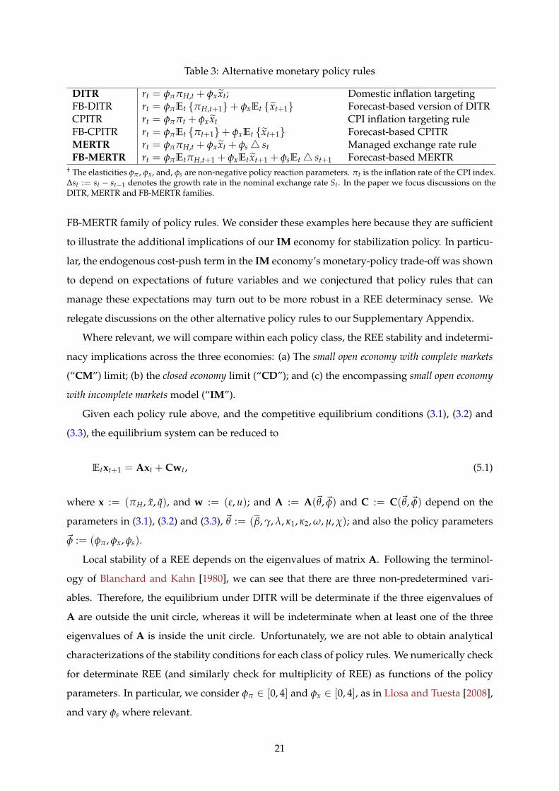
Table 3: Alternative monetary policy rules

DITR rt = φππH,t + φx xt; Domestic inflation targetingFB-DITR rt = φπEt πH,t+1+ φxEt xt+1 Forecast-based version of DITRCPITR rt = φππt + φx xt CPI inflation targeting ruleFB-CPITR rt = φπEt πt+1+ φxEt xt+1 Forecast-based CPITRMERTR rt = φππH,t + φx xt + φs4 st Managed exchange rate ruleFB-MERTR rt = φπEtπH,t+1 + φxEt xt+1 + φsEt4 st+1 Forecast-based MERTR

† The elasticities φπ , φx, and, φs are non-negative policy reaction parameters. πt is the inflation rate of the CPI index.∆st := st − st−1 denotes the growth rate in the nominal exchange rate St. In the paper we focus discussions on theDITR, MERTR and FB-MERTR families.

FB-MERTR family of policy rules. We consider these examples here because they are sufficient

to illustrate the additional implications of our IM economy for stabilization policy. In particu-

lar, the endogenous cost-push term in the IM economy’s monetary-policy trade-off was shown

to depend on expectations of future variables and we conjectured that policy rules that can

manage these expectations may turn out to be more robust in a REE determinacy sense. We

relegate discussions on the other alternative policy rules to our Supplementary Appendix.

Where relevant, we will compare within each policy class, the REE stability and indetermi-

nacy implications across the three economies: (a) The small open economy with complete markets

(“CM”) limit; (b) the closed economy limit (“CD”); and (c) the encompassing small open economy

with incomplete markets model (“IM”).

Given each policy rule above, and the competitive equilibrium conditions (3.1), (3.2) and

(3.3), the equilibrium system can be reduced to

Etxt+1 = Axt + Cwt, (5.1)

where x := (πH, x, q), and w := (ε, u); and A := A(~θ,~φ) and C := C(~θ,~φ) depend on the

parameters in (3.1), (3.2) and (3.3), ~θ := (β, γ, λ, κ1, κ2, ω, µ, χ); and also the policy parameters

~φ := (φπ, φx, φs).

Local stability of a REE depends on the eigenvalues of matrix A. Following the terminol-

ogy of Blanchard and Kahn [1980], we can see that there are three non-predetermined vari-

ables. Therefore, the equilibrium under DITR will be determinate if the three eigenvalues of

A are outside the unit circle, whereas it will be indeterminate when at least one of the three

eigenvalues of A is inside the unit circle. Unfortunately, we are not able to obtain analytical

characterizations of the stability conditions for each class of policy rules. We numerically check

for determinate REE (and similarly check for multiplicity of REE) as functions of the policy

parameters. In particular, we consider φπ ∈ [0, 4] and φx ∈ [0, 4], as in Llosa and Tuesta [2008],

and vary φs where relevant.

21

We will state the overall conclusions for our baseline model parametrisation. First, mar-

ket incompleteness results in an opposite conclusion to the finding in Llosa and Tuesta [2008].

Llosa and Tuesta [2008] showed that the set of admissible DITR (that respond to contemporane-

ous variables) inducing unique REE, in a small open economy with complete markets, is larger

than that in its closed-economy limit. In general, we find that market incompleteness makes

the admissible policy sets smaller than when we have the limit of the complete-markets small

open economy. In the specific case of the DITR, international asset market incompleteness also

reduces the admissible policy space relative to when we have the closed-economy limit. Sec-

ond, if the policy rules are of the forecast-based families (FB-DITR, FB-CPITR and FB-MERTR),

then market incompleteness in our model also shrinks the sets of these policies that can induce

unique REE, relative to their counterparts in the special case of the complete-markets small

open economy model. Third, if monetary policy can be described by simple policy rules, then

a contemporaneous rule (MERTR) that not only responds to domestic inflation and output gap,

but also to the real exchange rate growth, can greatly expand the feasible set of such policies in

inducing determinate rational expectations equilibrium. This result is also well-known in the

context of small open economies with complete markets [see e.g. Llosa and Tuesta, 2008].

DITR. Figure 1 reports the simulation results for DITR across the three economies, under the

baseline parametrization. Each shaded region refers to the set of DITR policy rules, indexed by

(φπ, φx), that would have induced a determinate (i.e. stable) REE in each of the economies CM,

CD, and IM. The complement set of each shaded region represents the region with multiple or

indeterminate REE.

[ Figure 1 about here. ]

Consider our baseline IM economy under the DITR family of policy rules. We observe that

the largest value of φπ for which REE indeterminacy arises is 1 which corresponds with φx = 0.

The largest value of φx for which we find indeterminacy is 4, which corresponds to φπ = 0.97.

In fact, the points (φπ, φx) = (0.97, 4) and (φπ, φx) = (1, 0) determine the length of the locus

in Figure 1 that separates the region of DITR policies that induce REE indeterminacy (i.e. to its

left) and region of DITR policies that induce REE stability (i.e. to its right).

From this figure, we can see that the monetary authority is not constrained if the policy

reaction to inflation φπ is larger than unity (i.e. the “Taylor principle”). However, provided

that φπ < 1, the smaller this policy parameter is, the greater the authority’s response to the

output gap.

22

Further, from Figure 1, we can see a qualification of existing results [e.g. Llosa and Tuesta,

2008] that openness to trade reduces indeterminacy of REE under the DITR family of policy

rules. Now, openness to trade under complete markets (CM) reduces the set of DITR policy that

induces REE indeterminacy, compared to the CD economy. However, incomplete asset markets

(IM) expands the set of indeterminate REE from that of the CD economy. This observation is

new to the literature. In other words, while trade openness reduces the constraint for DITR

policy makers if markets are complete, this openness increases the constraints if markets are

incomplete. However, note that the above result requires that the parametrization of the CRRA

parameter σ be “sufficiently large”.

The intuition for this is not surprising once we recall our observations in Section 4.2, and

in particular, Proposition 5. As discussed in Section 4.2, and also numerically verified in Table

2, market incompleteness does two things: (i) it exacerbates the slope of the inflation-output-

gap trade-off; and (ii) it amplifies the shifts to this trade-off due to the endogenous cost-push-

real-exchange-rate channel. The additional sensitivity of inflation to output gap and the real

exchange rate in the Phillips curve means that a DITR policy maker in the IM economy will

have to counter movements in inflation much more than its counterparts in the CM or CD

economies, in order to deliver a determinate REE. Finally, under CM, the trade-off is flatter

than under CD. Thus the same observation as in Llosa and Tuesta [2008] applies here: That for

a given response to domestic inflation, a CM-DITR policy intending to deliver a determinate

or stable REE needs to respond less heavily to output gap than its counterpart one in the CD

setting, provided that the expenditure switching channel is sufficiently strong, i.e. ση > 1.

For completeness, we also consider numerical examples where σ is “small”, and in partic-

ular, when σ = σ∗ (equivalence between IM and CM) or σ = σ (equivalence between CM and

CD). The numerical results are reported in Table 4. From Propositions 3 and 4, we can already

Table 4: Regions of DITR policies that induce REE indeterminacy—alternative cases of σ

IM CM CDσ Corners† (φπ , φx) Area‡ Corners† (φπ , φx) Area‡ Corners† (φπ , φx) Area‡

5 (baseline) (0.99, 0), (0.97, 4) 3.942 (1, 0), (0.67, 4) 3.336 (1, 0), (0.91, 4) 3.825σ = 0.67 (0.99,0), (0.79,4) 3.580 (1,0), (0.59,4) 3.160 (1,0), (0.59,4) 3.160σ∗ = 0.25 (0.99,0), (0.47,4) 2.923 (0.99,0), (0.47,4) 2.923 (1,0), (0.35,4) 2.6730.15 (0.99,0), (0.39,4) 2.754 (0.99,0), (0.39,4) 2.754 (1,0), (0.24,4) 2.4590.1 (0.99,0), (0.32,4) 2.614 (0.99,0), (0.32,4) 2.614 (1,0), (0.18,4) 2.322

† “Corners” refer to the two interior vertices of region of policies that yield indeterminate REE. See Figure 1 for an example ofthe baseline parametrization with σ = 5.‡ “Area” refers to the area of the polygonal region of policies that yield indeterminate REE. The sample policies in the relevantregion are given by the interior ”corners” and the origin (0, 0) and (0, 4) in (φπ , φx)-space.

expect the results for values of the CRRA parameter σ that are “too small”. The first row of

23

Table 4 is the baseline case across all three economies—i.e. the tabulation of Figure 1. Next,

consider the second row as an example, where σ = σ (equivalence between CM and CD). This

example shows that the regions of DITR policies that induce REE stability (or indeterminacy)

are identical for the CM and CD economies. Moreover, the area of indeterminacy for the IM

economy is larger. The intuition for this comes from observing that the policy trade-off in this

case for IM, κ IMσ = κCD

σ + σγ1−γ − κ2µ−1(1− γ) > κCD

σ ≡ κCMσ > 0 — i.e. it is steeper than the

equivalent CM and CD economies. We summarize the main finding above and its alternative

numerical results from Table 4 in the following three statements.

Result 1 Assume the DITR family of monetary policy rules. Comparing IM(σ) and the CM(σ) open

economies we observe that:

• If σ > σ∗ (i.e. κ2 < 0) then the set of DITR policy rules indexed by (φπ, φx) that would have

induced indeterminate (stable) REE is larger (smaller) in the IM(σ) economy.

• If σ ≤ σ∗ (i.e. κ2 ≤ 0) then the set of DITR policy rules indexed by (φπ, φx) that would have

induced indeterminate (or stable) REE is the same in IM(σ) and in CM(σ).

Result 2 Comparing the CD(σ) and the CM(σ) economies we observe that:

• If σ > σ, then the set of DITR policy rules indexed by (φπ, φx) that would have induced indeter-

minate (or stable) REE is smaller (larger) in the CM(σ) economy.

• If σ = σ, then the set of DITR policy rules indexed by (φπ, φx) that would have induced indeter-

minate (or stable) REE is the same in the CM(σ) economy and in the CD(σ) economy.

• If σ < σ, then the set of DITR policy rules indexed by (φπ, φx) that would have induced stable

(indeterminate) REE is larger (smaller) in the CD(σ) economy.

Result 3 Comparing the IM(σ) and the CD(σ) economies we observe that the set of DITR policy

rules that would have induced an indeterminate (stable) REE is always larger (smaller) in the open IM

economy.

These numerical results corroborate our theoretical insights from Propositions 3, 4 and 5

above. However, recall that some of these possibilities described above would be moot, from

a quantitative point of view, since one typically parametrizes σ ≥ 1, and for plausible calibra-

tions, we will have σ∗ < σ < σ < 1.

24

MERTR. Consider the Managed Exchange Rate Taylor Rule (MERTR). Using the definition

of the nominal exchange rate, ∆st = ∆qt + πt − π∗t , where without loss of generality we set

π∗t = 0, we then obtain the relation that ∆st =1

1−γ ∆qt +πH,t. Using this, we have an equivalent

representation of the MERTR as

rt = (φπ + φs)πH,t + φx xt +

(γφπ + φs

1− γ

)(qt − qt−1), (5.2)

By combining this rule with the equilibrium conditions for the IM economy, we can again

characterize REE stability numerically.

Similarly, we can derive a representation of the MERTR for the case of the CM economy as

rt = (φπ + φs)πH,t +

(φx +

τ(γφπ + φs)

1− γ

)xt −

τ(γφπ + φs)

1− γxt−1, (5.3)

where τ := σ(1−γ)(1−γ)2+σηγ(2−γ)

.

We fix φs = 0.6 as in Llosa and Tuesta [2008].16 Relative to the DITR, the admissible set

of the MERTR inducing determinate REE equilibrium is larger. However, relative to the CM

economy, asset market incompleteness in the IM economy reduces this set.

[ Figure 2 about here. ]

An interesting observation about this policy is its equivalence to one that also responds

to a quasi-difference in output gap growth in the CM economy. One can interpret this as a

policy that places a limit on the speed in the domestic-inflation-output-gap trade-off. It does

so by responding to a measure of output gap growth and growth in the domestic-goods price

level; and it thus is able to prevent a self-fulfilling prophecy spiral in unstable inflation. This

is achieved to a lesser degree by (5.2) in the IM economy, since it still faces a larger policy

trade-off. However, compared to the DITR policy, now the MERTR family of policies deal

with managing real exchange rate growth directly. By doing so, the policies can better regular

expectations of output gap and real exchange rates. The latter expectational variables feature in

the composition of the endogenous cost-push shock term vt in the policy trade-off (4.10). Thus

preventing a self-prophesying spiral in these variables through the endogenous cost-push term

is crucial. This point is made stronger if we contrast with the next class of policy rules that

attempt to manipulate expectations directly.

16Additional sensitivity results with respect to φs are available from the authors. We show that the qualitativeordering of the sets of determinate or indeterminate equilibria are not affected by the feasible choice of this param-eter.

25

FB-MERTR. It can be shown that the FB-MERTR rule has an equivalent form of

rt = (φπ + φs)EtπH,t+1 + φxEt xt+1 +

(γφπ + φs

1− γ

)(Etqt+1 − qt), (5.4)

in the IM economy, and,

rt = (φπ + φs)EtπH,t+1 +

[φx + τ

(γφπ + φs

1− γ

)]Et xt+1 − τ

(γφπ + φs

1− γ

)xt, (5.5)

in the CM economy, where τ := σ(1−γ)(1−γ)2+σηγ(2−γ)

.

Relative to CM economy, asset market incompleteness in the IM economy results in a

smaller admissible set of the FB-MERTR inducing determinate REE equilibrium.

[ Figure 3 about here. ]

This example policy illustrates our intuition in Section 4.2 most starkly. Now, instead of

responding to real exchange rate growth, the policy responds to expectations of real exchange

rate growth, inter alia. By doing so, we can see that this family of policies is less capable

of delivering stable REE. The intuition is that by responding directly to expections of future

variables, this exacerbates further the already larger domestic-inflation-output-gap trade-off in

the IM economy (relative to CM), by causing more self-fulfilling spirals in exchange rate and

inflation expectations, amplified through the endogenous cost-push term vt in (4.10).

Discussion. We have seen in the illustrations above, for a quantitatively plausible risk aver-

sion σ, that the existence of incomplete international risk sharing results in a reduction of the

sets of admissible rules inducing determinate REE, relative to when the environment is the

standard complete-markets small open economy; and where relevant, relative to when the

environment is the standard closed economy. However, given international asset market in-

completeness, the admissible set of stabilizing policy rules can be greatly expanded by a family

of simple policies that take into account contemporaneous real exchange rate growth as well.

In the Supplementary Appendix, we also discuss a similar result (with similar intuitions) for

the class of the CPITR rule.

These results make sense, since the additional constraints on policy in the incomplete-

markets setting, arose through: (i) an exacerbated conditional trade-off between domestic in-

flation and output gap; and (ii) the endogenous cost-push channel. As hinted earlier in Section

4.2, the latter gave us another means of preventing self-fulfilling multiple equilibria, or worse,

equilibrium instability. This other means is effected through monetary policies that can “cor-

rectly” manage expectations that affect the endogenous cost-push term. By smoothing out

26

output gap and real exchange rates, it turns out that the CPITR and better yet, the MERTR poli-

cies are better at inducing a determinate rational expectations equilibrium. This is perhaps one

reason why practising small-open-economy inflation targeters do worry about exchange rate

management in the monetary policy designs.

6 Concluding remarks

In this paper, we have developed a small open economy whose monetary policy implications

are no longer similar to its closed-economy counterpart. We showed, in a transparent manner,

that asset market incompleteness essentially exposes the supply side of the model’s equilibrium

characterization to a notion of an endogenous cost-push shock. Our notion of an endogenous

cost-push trade-off here is different to existing models with complete markets [c.f. Monacelli,

2005]. In our model, this is a consequence of an irreducible and explicit exchange rate equi-

librium dynamic channel. Moreover, this term involves endogenous random variables that

comprise conditional expectations of future output gap and real exchange rate gap. We then

showed how this alters the relevant monetary-policy trade off between stabilizing domestic in-

flation and stabilizing output gap in an analytical and comparative way. Finally, we re-visit the

lessons on equilibrium determinacy under alternative rules in a small open economy. We show

that asset market incompleteness now results in opposite conclusions to the existing literature

utilizing the workhorse complete markets model.

While our model is a simple and transparent illustration of the relation between interna-

tional asset market incompleteness, equilibrium exchange rate irreducibility, and its implica-

tions for monetary policy trade-off and rational expectations equilibrium determinacy, it is

probably too simple for normative business-cycle and welfare analysis. These questions have

been addressed by larger and more quantitative models [see e.g. de Paoli, 2009b; Monacelli,

2005].

References

Benigno, Gianluca and Christoph Thoenissen, “Consumption and Real Exchange Rates with Incom-plete Markets and Non-traded Goods,” Journal of International Money and Finance, October 2008, 27 (6),926–948. Cited on page(s): [4], [5], [6]

and Pierpaolo Benigno, “Price Stability in Open Economies,” Review of Economic Studies, October2003, 70 (4), 743–764. Cited on page(s): [2], [11]

Blanchard, Olivier and Charles M. Kahn, “The Solution of Linear Difference Models under RationalExpectations,” Econometrica, 1980, 48, 1305–1311. Cited on page(s): [21], [14]

Bullard, James and Kaushik Mitra, “Learning About Monetary Policy Rules,” Journal of Monetary Eco-nomics, 2002, 49, 1105–1129. Cited on page(s): [4], [19], [20], [13]

27

Chari, V V, Patrick J Kehoe, and Ellen R McGrattan, “Can Sticky Price Models Generate Volatile andPersistent Real Exchange Rates?,” Review of Economic Studies, July 2002, 69 (3), 533–63. Cited onpage(s): [4], [5]

Clarida, Richard, Jordi Galı, and Mark Gertler, “The Science of Monetary Policy: A New KeynesianPerspective,” Journal of Economic Literature, December 1999, 37 (4), 1661–1707. Cited on page(s): [10],[11]

, , and , “Optimal Monetary Policy in Open Versus Closed Economies: An Integrated Approach,”AEA Papers and Proceedings, 2001, 91 (2), 248–252. Cited on page(s): [2], [3], [8], [10], [11], [12], [13],[17], [7]

de Paoli, Bianca, “Monetary Policy and Welfare in a Small Open Economy,” Journal of International Eco-nomics, 2009, 77 (1), 11–22. Cited on page(s): [11]

, “Monetary Policy under Alternative Asset Market Structures: The Case of a Small Open Economy,”Journal of Money, Credit and Banking, October 2009, 41 (7), 1301–1330. Cited on page(s): [2], [4], [27]

Ferrero, Andrea, Mark Gertler, and Lars E. O. Svensson, “Current Account Dynamics and MonetaryPolicy,” in Jordi Galı and Mark Gertler, eds., International Dimensions of Monetary Policy, University ofChicago Press 2010, pp. 199–244. National Bureau of Economic Research Conference Report. Citedon page(s): [6], [10], [3]

Galı, Jordi and Tommaso Monacelli, “Monetary Policy and Exchange Rate Volatility in a Small OpenEconomy,” Review of Economic Studies, 2005, 72 (3), 707–734. Cited on page(s): [2], [3], [6], [7], [8], [10],[11], [19], [20], [4], [12]

Leitemo, Kai and Ulf Soderstrom, “Robust Monetary Policy in a Small Open Economy,” Journal ofEconomic Dynamics and Control, October 2008, 32 (10), 3218–3252. Cited on page(s): [4]

Linnemann, Ludger and Andreas Schabert, “Net foreign assets, interest rate policy, and macroeco-nomic stability,” Technical Report 54, Money Macro and Finance Research Group September 2004.Cited on page(s): [4], [6]

Llosa, Luis-Gonzalo and Vicente Tuesta, “Determinacy and Learnability of Monetary Policy Rulesin Small Open Economies,” Journal of Money, Credit and Banking, 2008, 40 (5), 1033–1063. Cited onpage(s): [3], [4], [8], [19], [20], [21], [22], [23], [25], [11], [13], [14]

Lubik, Thomas A., “Non-stationarity and instability in small open-economy models even when theyare ‘closed’,” Economic Quarterly, 2007, Fall, 393–412. Cited on page(s): [6]

McCallum, Bennett T. and Edward Nelson, “Nominal Income Targeting in an Open-economy Optimiz-ing Model,” Journal of Monetary Economics, 1999, 43, 553–578. Cited on page(s): [4], [5], [6], [8], [19],[20], [11]

Monacelli, Tommaso, “Monetary Policy in a Low Pass-Through Environment,” Journal of Money, Creditand Banking, 2005, 37 (6), 1047–1066. Cited on page(s): [2], [11], [27]

Schmitt-Grohe, Stephanie and Martın Uribe, “Closing Small Open Economy Models,” Journal of Inter-national Economics, October 2003, 61 (1), 163–185. Cited on page(s): [6]

Woodford, Michael, Interest and Prices: Foundations of a Theory of Monetary Policy, Princeton, NJ: Prince-ton University Press, 2003. Cited on page(s): [3], [12]

28

Figure 1: Domestic inflation targeting rule (DITR) and indeterminacy regions(shaded) for three economies. Each complementary region refers to stable REEcases.

29

Figure 2: Managed exchange rate targeting rule (MERTR) and indeterminacy forthree economies. Each complementary region refers to stable REE cases.

30

Figure 3: Forecast-based managed exchange rate targeting rule (FB-MERTR) andindeterminacy for three economies. Each complementary region refers to stableREE cases.

31

Supplementary Appendix

Anatomizing Incomplete-markets Small Open Economies: Policy

Trade-offs and Equilibrium Determinacy

Jaime Alonso-Carrera† and Timothy Kam∗

Not for publication

A Derived demand and pricing functions

Continuing from Section 2.1, recall that each optimally chosen Ct will be consistent with the household’s

intra-period choice of a home-produced final consumption good, CH,t and an imported final good CF,t,

where Ct is defined by a CES aggregator

Ct =

[(1− γ)

1η (CH,t)

η−1η + γ

1η (CF,t)

η−1η

] ηη−1

; γ ∈ (0, 1), η > 1.

Each type of final good, CH,t and CF,t, aggregates a variety of differentiated goods indexed by i, j ∈

[0, 1]: CH,t =[∫ 1

0 CH,t (i)ε−1

ε di] ε

ε−1, and CF,t =

[∫ 10 CF,t (j)

ε−1ε dj

] εε−1

, where ε > 1. Static expenditure

minimization by consumers result in the demand functions:

CH,t (i) =(

PH,t (i)PH,t

)−ε

CH,t, CF,t (j) =(

PF,t (j)PF,t

)−ε

CF,t (A.1)

for all i, j ∈ [0, 1], where the aggregate price levels are solved as

PH,t =

(∫ 1

0PH,t (i)

1−ε di) 1

1−ε

, PF,t =

(∫ 1

0PF,t (j)1−ε dj

) 11−ε

. (A.2)

Likewise, optimal consumption demand of final home and foreign goods can be derived, respectively,

as

CH,t = (1− γ)

(PH,t

Pt

)−η

Ct, CF,t = γ

(PF,t

Pt

)−η

Ct.

Substitution of these demand functions into (2.7) yields the consumer price index as

Pt =[(1− γ) P1−η

H,t + γP1−ηF,t

] 11−η . (A.3)

B Optimal price-setting

We assumed in the paper a function R+ 3 Cat 7→ β(Ca

t ) ∈ (0, 1) that represents endogenous (aggregate

consumption dependent) one-period discounting. Note that for a fixed sequence of aggregate consump-

tion Caτk−1

τ=0 the k-period ahead endogenous discount factor is ∏k−1τ=0 β(Ca

τ), where β(Ca0) = 1.

B.1 The Calvo-style pricing problem

The monopolistically competitive firm i ∈ [0, 1] chooses pricing strategy PH,t(i, ht). Given Markovian

public histories of states, ht := z0, ..., zt, we further restrict the optimal pricing strategy to belong to a

class induced by stationary pricing decision functions PH,t such that PH,t(i, zt[ht]) = PH(i, zt).

Let the aggregate price in the home goods industry H, in time t+ k and state zt+k, be PH,t+k(zt+k) :=

PH,t+k. The aggregate domestic and foreign consumption demands are, respectively, CH,t+k(zt+k) :=

CH,t+k and C∗H,t+k(zt+k) := C∗H,t+k. The output of firm i in that state and date is then Yt+k(i, zt+k) :=

1

Yt+k(i). The demand faced by firm i in state zt+k, if the price PH,t(i, zt) := PH,t(i) still prevails (with

probability θk) in period t + k is given by

Yt+k(i) =(

PH,t(i)PH,t+k

)−ε [CH,t+k + C∗H,t+k

], (B.1)

where we have suppressed the explicit state-dependence notation.

Let ξt := UC[C(zt)]. The firm i solves the following expected total discounted nominal profit maxi-

mization problem:

maxPH,t(i)

∞

∑k=0

Et

(t+k−1

∏τ=t

β(Caτ)

)ξt+1

ξt

[PH,t(i)−MCn

t+k]

Yt+k(i)

, (B.2)

subject to (B.1).

B.2 Optimal pricing plan in a symmetric pricing equilibrium

The first order condition with respect to PH,t(i) is

Et

∞

∑k=0

θk

(t+k−1

∏τ=t

β(Caτ)

)ξt+kξt

Yt+k(i)[

PH,t(i)−(

ε

ε− 1

)MCn

t+k

]= 0. (B.3)

We re-write the problem in real terms, by dividing both sides of (B.3) with the aggregate home-goods

price level, PH,t:17

Et

∞

∑k=0

θk

(t+k−1

∏τ=t

β(Caτ)

)ξt+kξt

Yt+k(i)[

PH,t(i)PH,t

−(

ε

ε− 1

)(PH,t+k

PH,t

)MCt+k

]= 0. (B.4)

where real marginal cost in time t + k and state zt+k is MCt+k =:MCn

t+kPH,t+k

. We restrict attention to a

symmetric pricing equilibrium.

Definition 2 A symmetric pricing equilibrium is a stationary Markovian strategy such that PH,t(i, zt)∞t=0 =

PH,t(zt)∞t=0 for all firms i ∈ [0, 1] that reset prices at time t, and PH,t(zt)∞

t=0 satisfies (B.4).

C Deriving the log-linear equilibrium system

In this appendix we provide the details of the log-linearization of the three key conditions that locally

approximate the equilibrium characterizations of recursive equilibrium in the model.

17This also renders the characterization of optimal pricing in terms of stationary variables.

2

C.1 Optimal consumer plan and UIP

By log linearizing the previous conditions (2.4), (2.5) and (2.6), and by imposing the equilibrium condi-

tion Ct = Cat , we obtain that the optimal consumer’s plan is approximately characterized by:18

σct = wt − pt − ϕnt, (C.1)

− (σ− φ) ct = rt −Et πt+1 − σEt ct+1+ φϑ, (C.2)

− (σ− φ) ct = r∗t − qt + Et qt+1 − σEt ct+1+ φϑ, (C.3)

where qt denotes the percentage deviation from steady state of the real exchange rate Qt; πt+1 is the

rate of change in the domestic consumer price index from t to t + 1, i.e., πt+1 = pt+1 − pt; and r∗t is

the foreign interest rate, i.e., r∗t = i∗t − Et

π∗t+1

, with π∗t+1 denoting the inflation rate of the foreign

consumer price index. Without loss of generality, we will assume that r∗t is just a (linear) function of

y∗t .19 In order to maintain the same sign of slope of the Euler equation as in Galı and Monacelli [2005]

we will require that σ− φ > 0. This requirement is consistent with our assumption, following Ferrero et

al. [2010], on the subjective discount factor (φ 0) and that is has negligible qualitative and quantitative

consequences on the monetary policy problem.

The log-linear form for the consumption index (2.7) is given by:

ct = (1− γ) cH,t + γcF,t, (C.4)

where cH,t is also an index of consumption of domestically produced goods; cF,t is an index of imported

goods; and γ ∈ [0, 1] measures the degree of openness. The domestic consumer price index (A.3) is

log-linearized as

pt = (1− γ) pH,t + γpF,t, (C.5)

where pH,t is the price index for domestically produced goods; and pF,t is the price index for imported

goods. Similarly, domestic output in log- linear form is given in equilibrium by

yt = (1− γ) cH,t + γc∗H,t, (C.6)

where c∗H,t is the export of domestically produced goods. The optimal allocation of expenditure within

18Henceforth, lower-case letters will denote the logarithms of the corresponding upper-case variables.19It has been shown in Galı and Monacelli [2005] that if we assume the rest of the world as a limiting closed

economy under a first-best and flexible price competitive equilibrium, then y∗t is equal to its potential output. Thatis y∗t is approximately a linear function of its exogenous technology a∗t , y∗t = b(θ)a∗t , where b(θ) denotes a scalarfunction of the closed economy’s underlying taste and technology parameters θ. Thus it suffices to characterize theapproximate equilibrium solution of this model as linear functions of (at, y∗t ).

3

each category of goods yields the following demands:

cH,t = η (pt − pH,t) + ct, (C.7)

cF,t = η (pt − pF,t) + ct, (C.8)

c∗H,t = η (st + p∗t − pH,t) + c∗t . (C.9)

We assumed that the law of one price holds at all periods, so that pF,t = st + p∗t . Combining this

expression with the consumption price index (C.5) and the definition of the real exchange rate, we

obtain that

pt − pH,t =

(γ

1− γ

)qt. (C.10)

From this equation we directly follow that the rate of change in the price index of the domestically

produced goods (or domestic inflation) differs from the inflation rate of the domestic consumer price

index. In particular we obtain that

πt − πH,t =

(γ

1− γ

)(qt − qt−1) , (C.11)

where πH,t is the domestic inflation rate. Observe that the gap between the two inflation rates is propor-

tional to the variation in the real exchange rate, with the degree of proportionality determined by the

degree of openness γ.

By combining (C.10) with (C.6), (C.7) and (C.9), we obtain that domestic output is equal to

yt = (1− γ) ct +

[ηγ (2− γ)

1− γ

]qt + γy∗t , (C.12)

where we have used the fact that the foreign economy is large, which implies that the weight in the

foreign composite consumption C∗t of the domestic goods is negligible, so that y∗t = c∗t .

C.1.1 The UIP condition and incomplete international risk sharing

From the optimality conditions for the consumers’ problem we can derive the uncovered interest parity

(UIP) condition. More specifically, from the conditions (C.2) and (C.3) we obtain the following log-linear

approximation of the UIP condition:

rt = r∗t + Et πt+1 − qt + Et qt+1 . (C.13)

Under complete markets the Euler equations of the domestic and the foreign countries provide a tight

state-by-state and date-by-date relation linking domestic consumption with foreign consumption and

real exchange rate[see. e.g. Galı and Monacelli, 2005]. In particular, under our utility function (2.2)

this relationship is in log-linear terms given by: ct = c∗t +(

1σ

)qt. This implies that the dynamics of

output and the real exchange rate are perfectly correlated. However, this is no longer true in the case

4

of incomplete asset markets. As Chari et al. [2002] show, in this case the relation between real exchange

rate and consumption only holds in conditional expectation terms. In particular, combining condition

(C.3) with the Euler equation of the foreign economy yields

Et qt+1 − qt =[σEt

y∗t+1

− (σ− φ) y∗t

]− [σEt ct+1 − (σ− φ) ct] , (C.14)

where we have also used the condition y∗t = c∗t . Therefore, output and real exchange are not perfect

correlated, so that we need equation (C.13) to characterize the full equilibrium dynamics of our model

as we will show below [see also ?Benigno and Thoenissen, 2008].

Using (C.13) and (C.11), we obtain the following dynamic equation for the gap in the real exchange

rate, as found in the main paper:

qt = Et qt+1 − (1− γ) [rt −Et πH,t+1] + ut. (3.3)

C.2 Approximating the supply side

Log-linearizing (2.8) around the zero-inflation steady state, we obtain that the aggregate output in loga-

rithmic terms is given by

yt = at + nt, (C.15)

Moreover, from cost minimization we obtain

nt = yt + [mct − (wt − pt) + (pH,t − pt)] , (C.16)

where mct := ln(MCnt /PH,t)− ln[(1− ε)/ε] is the percentage deviation in real marginal cost from steady

state.

C.2.1 Real marginal cost

By combining (2.9) with (C.1), (C.12), (C.15) we get

mct =

[σ + ϕ (1− γ)

1− γ

]yt +

[γ

(1− γ)− σηγ (2− γ)

(1− γ)2

]qt − (1 + ϕ) at −

(γ(1 + ϕ)

1− γ

)y∗t

.(C.17)

In the flexible price equilibrium, we obtain that

0 =

[σ + ϕ (1− γ)

1− γ

]yt +

[γ

(1− γ)− σηγ (2− γ)

(1− γ)2

]qt − (1 + ϕ) at −

(γ(1 + ϕ)

1− γ

)y∗t

.(C.18)

5

Subtracting (C.18) from (C.17) we obtain real marginal cost deviations as a function output gap and real

exchange rate gap deviations:

mct =

[σ + ϕ (1− γ)

1− γ

]xt +

[γ

(1− γ)− σηγ (2− γ)

(1− γ)2

]qt

. (C.19)

C.2.2 Optimal pricing policy function

For small perturbations around a zero-inflation steady state, (B.4) can be approximated to first-order

accuracy as:

Et

∞

∑k=0

[β (Cass) θ]k ξssYss(i)

[pH,t − ln

(PH,t+k

PH,t

)−mct+k

], (C.20)

where

pH,t := ln(

PH,t

PH,t

), mct := ln

(MCn

tPH,t

)− ln

(ε− 1

ε

).

Define PH,t = ln(PH,t/PH,ss). So then (C.20) can be re-written as

(1

1− β (Cass) θ

)pH,t = Et

∞

∑k=0

[β (Cass) θ]k

[PH,t+k + mct+k

]−(

11− β (Ca

ss) θ

)PH,t

⇒ pH,t + PH,t = (1− β (Cass) θ)Et

∞

∑k=0

[β (Cass) θ]k

[PH,t+k + mct+k

].

By the law of iterated expectations, this can be written recursively as

pH,t + PH,t = [1− β (Cass)]

(PH,t + mct

)+ [β (Ca

ss) θ]Et(

pH,t+1 + PH,t+1)

⇒ pH,t = [1− β (Cass) θ]mct + [β (Ca

ss) θ]Et ( pH,t+1 + πH,t+1) . (C.21)

Recall that in the ?-style model, by the law of large numbers, the evolution of the aggregate home goods

price level is such that

P1−εH,t = (1− θ)P1−ε

H,t + θP1−εH,t−1.

A log-linear approximation of this yields a linear relationship between home goods price inflation,

πH,t := ln(PH,t/PH,t−1) and the percentage deviation of the optimal price from the aggregate price

level:

πH,t =1− θ

θpH,t.

6

Using this identity, and the one-period ahead forecast of the same identity, in (C.21), we obtain the

characterization of the approximately log-linear optimal pricing function pH,t in terms of a forward-

looking Phillips curve:

πH,t = βEt πH,t+1+[(1− θ)

(1− θβ

)θ

]mct, (C.22)

with β := β(Css), where Css is the level of domestic consumption at the zero-inflation steady state.

Combining (C.22) with (C.19), we obtain

πH,t = βEt πH,t+1+ λ (κ1 xt + κ2qt) , (3.1)

where

λ =

[(1− θ)

(1− θβ

)θ

],

κ1 = ϕ +σ

1− γ, κ2 = −σηγ(2− γ)

(1− γ)2 +γ

(1− γ).

Equation (3.1) is almost identical, to first-order accuracy, to the Phillips curve derived in models such

as Galı and Monacelli [2005] and Clarida et al. [2001]. What is different is that the one-period discount

factor at the deterministic steady state is now a function of fundamental outcomes in the steady-state

competitive equilibrium. In this case, it will be a function of steady-state aggregate consumption, Css.

More generally, if we do not focus on local linearized dynamics around the deterministic steady state, the

global dynamics of inflation will also depend non-linearly on the endogenous discount factor function

β : R+ → (0, 1).

As in the closed economy a change in the domestic output has a positive effect on the domestic

inflation rate. In our model the size of this effect depends on the degree of openness γ and on the

productive dependence α (or, equivalently, δ). An increase in the domestic output has an effect on the

marginal cost through: (i) an increase in the equilibrium level of employment, that is captured by the first

term ϕ in κ1; (ii) a rise in the terms of trade given by the second term in κ1, which is negatively related

with the degree of opennes γ; and (iii) an increase in the equilibrium level of the imported intermediate

good given by the second term in λ, which is positively related with the productive dependence α (or,

equivalently, δ).

7

C.3 Approximating the demand side

By combining (C.2) with (C.11) and (C.12), we obtain after some simple algebra that

yt =

(σ

σ− φ

)Et yt+1 −

(1− γ

σ− φ

)[it −Et πH,t+1]

+

[γ

σ− φ− σηγ (2− γ)

(1− γ) (σ− φ)

]Et qt+1

−[

γ

σ− φ− ηγ (2− γ)

1− γ

]qt −

(σγ

σ− φ

)Et

y∗t+1+ γy∗t

−φϑ(1− γ)

σ− φ(C.23)

C.4 Potential output and real exchange rate derivations

Here, we show that the potential output yt and real exchange rate qt are affine functions of exogenous

random technology and foreign output, respectively, at and y∗t .

We first charaterize the equilibrium when prices are fully flexible, i.e., mct = 0. From (C.1), (C.15),

and (2.9),we obtain that the equilibrium with flexible prices

σct + ϕyt +

[γ

1− γ

]qt − (1 + ϕ) at = 0. (C.24)

Moreover, combining the last equation with (C.12), we also obtain

ct = Ω1at −Ω2qt −Ω3y∗t , (C.25)

where

Ω1 =1 + ϕ

σ + ϕ (1− γ),

Ω2 =

[1

σ + ϕ (1− γ)

]and

Ω3 =γϕ

σ + ϕ (1− γ).

Using (C.25) and (C.14), we derive that

qt =

[(1− σΩ2)

1− (σ− φ)Ω2

]Et

qt+1

+

[Ω1

1− (σ− φ)Ω2

][σEt at+1 − (σ− φ) at]

−[

1 + Ω3

1− (σ− φ)Ω2

] [σEt

y∗t+1

− (σ− φ) y∗t

].

Hence, by solving forward the previous dynamic equation, we can see that the level of qt at the friction-

less equilibrium only depends on the exogenous stochastic variables at and y∗t . From (C.24) and (C.25)

8

we check that the previous conclusion is also true for the case of the levels of yt and ct.

From (C.18) and (C.23) we can derive the following condition on the equilibrium with flexible prices:

yt =

(σ

σ− φ

)Et

yt+1

−[

1− γ

σ + ϕ (1− γ)

] [γ

(1− γ)− σηγ (2− γ)

(1− γ)2

]qt

+

[σ (1− γ)

(σ− φ) [σ + ϕ (1− γ)]

]×[

γ

(1− γ)− σηγ (2− γ)

(1− γ)2

]Et

qt+1

+

[(1− γ) (1 + ϕ)

σ + ϕ (1− γ)

]at −

[σ (1− γ) (1 + ϕ)

(σ− φ) [σ + ϕ (1− γ)]

]Et at+1

+

[σγ

σ + ϕ (1− γ)

]y∗t −

[γσ2

(σ− φ) [σ + ϕ (1− γ)]

]Et

y∗t+1

. (C.26)

It is straightforward to deduce that yt will just be a linear function in (at, y∗t ).

C.5 Deriving the output gap IS relation

Subtracting (C.26) from (C.23), we obtain

xt =

(σ

σ− φ

)Et xt+1 −

[γ

σ− φ− ηγ (2− γ)

1− γ

]qt

+

[γ

σ− φ− σηγ (2− γ)

(1− γ) (σ− φ)

]Et qt+1

−(

1− γ

σ− φ

)[it −Et πH,t+1] + ξt, (C.27)

with

ξt =

[ηγϕ (2− γ)

σ + ϕ (1− γ)+

(1− γ

σ + ϕ (1− γ)

)γ

(1− γ)− γ

σ− φ

]qt

+

[γ

σ− φ− σηγϕ (2− γ)

(σ− φ) [σ + ϕ (1− γ)]

−(

σ

σ− φ

)(1− γ

σ + ϕ (1− γ)

)γ

(1− γ)

]Et

qt+1

−[(1− γ) (1 + ϕ)

σ + ϕ (1− γ)

]at +

[σ (1− γ) (1 + ϕ)

(σ− φ) [σ + ϕ (1− γ)]

]Et at+1

−[

γϕ (1− γ)

σ + ϕ (1− γ)

]y∗t +

[γσϕ (1− γ)

(σ− φ) [σ + ϕ (1− γ)]

]Et

y∗t+1− φϑ (1− γ)

σ− φ,

where ξt is a stochastic, exogenous variable as can be followed from the previous characterization of the

frictionless equilibrium. Finally, by introducing (3.3) into (C.27), we directly obtain equation (3.2) in the

main text, where

εt = ξt −[

γ

σ− φ− ηγ (2− γ)

1− γ

]ut.

9

D Generalized IM Model

Consider a generalized version of the IM model. Now, the only addition is that each domestic firm

i ∈ [0, 1] produces a differentiated good using a CES technology

Yt(i, ht) = α

[AtNd

t(i, ht)]ν

+ (1− α)[IMt

(i, ht)]ν

1ν

; α ∈ (0, 1],−∞ ≤ ν ≤ 1, (D.1)

where Ndt (i, ht) is labor hired by the firm; and IMt(i) is an index of imported intermediate goods.20 the

random variable At := expat is an exogenous embodied labor productivity.

The production cost-minimization problem for the firm is:

min Pt(ht) Qt

(ht) IMt

(i, ht)+ Wt

(ht)

Pt (ht)Nd

t(i, ht) .

subject to (2.8). The first-order conditions with respect to optimal labor and intermediate-imports are

Wt(ht)

Pt (ht)= α

MCnt(ht)

Pt (ht)Aν

t

(Yt(ht) (i, ht)

Ndt (i, ht)

)1−ν

,

and

Qt(ht) = (1− α)

MCnt(ht)

Pt (ht)

(Yt(i, ht)

IMt (i, ht)

)1−ν

,

respectively, where MCnt is nominal marginal cost.

With a homogeneous of degree one production function the first-order conditions (for cost mini-

mization with respect to labor) can be written in the aggregate as

Wt(ht)

Pt (ht)= α

MCnt(ht)

Pt (ht)Aν

t

(Yt(ht)

Ndt (ht)

)1−ν

(D.2)

and

Qt(ht) = (1− α)

MCnt(ht)

Pt (ht)

(Yt(ht)

IMt (ht)

)1−ν

, (D.3)

where MCnt is nominal marginal cost.

After some derivations, it can be shown that the REE for this economy is summarized by the follow-

ing definition.

Definition 3 (General Incomplete Markets (IM)) Given a monetary policy process rtt∈N and exogenous

processes εt, utt∈N, a (locally approximate) rational expectations competitive equilibrium (REE) in the IM

20This intermediate good can be interpreted as two equivalent forms. On the one hand, we can assume thatthe imported goods can be either devoted to consumption CF,t or used as a production input IMt. On the otherhand, we can assume that the domestic economy imports two differentiated goods: consumption goods CF,t andintermediated goods IMt.

10

model is a bounded stochastic process πH,t, xt, qtt∈N satisfying:

πH,t = βEt πH,t+1+ λ (κ1 xt + κ2qt) , (D.4)

xt = vEt xt+1 − µ [rt −Et πH,t+1] + χEt qt+1+ εt, (D.5)

qt = Et qt+1 − (1− γ) [rt −Et πH,t+1] + ut. (D.6)

where β = β(Css),

λ =(1− ν)(1− δ)

1− ν + δϕ

[(1− θ)

(1− θβ

)θ

],

κ1 = ϕ +σ

1− γ, κ2 =

δ(1− ν + ϕ)

(1− γ)(1− ν)(1− δ)− σηγ(2− γ)

(1− γ)2 +γ

(1− γ);

v =σ

σ− φ, µ =

[1− γ

σ− φ

] [1− γ +

ηγ (2− γ) (σ− φ)

1− γ

], and, χ =

ηγφ (2− γ)

(1− γ) (σ− φ);

where δ = (1− α)(IMss/Yss)ν, with IMss and Yss as the stationary values of imported intermediate good and

aggregate output, respectively.

D.1 Parameters in the general IM model

The generalized IM economy is parametrized in line with Llosa and Tuesta [2008] and McCallum and

Nelson [1999]. Llosa and Tuesta [2008] use the same parametrization as Galı and Monacelli [2005] with

the exception of the constant relative risk aversion coefficient (σ), the inverse of Frisch labor supply

elasticity (ϕ), and the elasticity of substitution between domestic and foreign goods (η). For a majority

of parameters, we follow that of in Llosa and Tuesta [2008] for two reasons: (i) Ease of comparison of

their findings with ours in terms of the REE stability analyses; and (ii) The setting in Llosa and Tuesta

[2008] is a more general parametrization. Furthermore, these parameters does not affect qualitatively

the results, although they may have important quantitative effects. This is especially true in the case

of σ.21 The parameter v is from McCallum and Nelson [1999]. We summarize the model parameters in

Table 1.

[ Table 1 about here. ]

Note that this set of parameters is later used to consider the limits of our model. That is, by using the

relevant composite parameters, we have: (i) The small open economy with complete markets (“CM”):

κ2 = 0, κ1 = κc1 and µ = µc; and, (ii) The closed economy (“CD”): γ = 0 and α = 1 (i.e., δ = 0).

21The goal in this paper is to understand the qualitative implications of incomplete markets on equilibriumstability using a simple but salient model, and not to quantify or match business cycle regularities. However, wedo perform some sensitivity analysis in this parameter when it would be required. Results of these alternativeexperiments will be readily made available upon request.

11

D.2 Numerical values of equilibrium relations

By using our baseline parametrization we can now sign the reduced-form parameters in the equilibrium

relations between variables in the approximation of the competitive equilibrium (3.1), (3.2) and (3.3). We

report this in Table 5.

[ Table 5 about here. ]

Recall that the only unclear equilibrium relation (in terms of sign or direction) is the slope of output

gap with respect to the real exchange rate in the Phillips curve (3.1), given by λκ2. From a Mundell-

Fleming-type intuition, one should expect that without imported inputs this value should be negative.

We show that in our baseline economy, this value is also negative with imported inputs. In fact, we

obtain that κ2 is positive if and only if v ∈ (0.92337, 1). Therefore, the aforementioned income effects of

the exchange rate variations dominates.

At this point, it is convenient to enumerate the differences between the incomplete market version

and the complete market version in terms of equilibrium relations. Remember that these differences are

in the relations λκ1, λκ2 and µ. Table 2 reports the differences across the economies with and without

openness in production, and with and without market incompleteness.

[ Table 6 about here. ]

From Table 2 we conclude the following. First, the positive trade-off between domestic inflation

and output gap, given by λκ1, is much larger (i.e. around six times larger) with incomplete markets,

regardless of the presence of an imported intermediate input channel (indexed by δ). The intuition is

quite standard. In the absence of complete international risk sharing, a given external shock to the small

open economy cannot be fully insured against by the single incomplete market claim. Hence the effect

of the shock gets amplified or transmitted more to domestic allocations via the inflation process.

Second, the relationship between domestic-goods inflation rate and output gap, given by λκ1, is

decreasing with δ (openness in production). Observe the Phillips curve relation in (3.1). Since there

is some substitutability in the inputs in the production technology, more reliance (i.e. higher δ) on the

imported intermediate input means a substitution away from the labor input, such that all else equal,

the effect of the labor cost channel on the inflation-real marginal-cost channel via λκ1 is then smaller.

Third, the relationship between domestic-goods inflation rate and output gap, given by λκ1, in the

closed economy (“CD”) is between the value in the incomplete market version and the complete market

version.

Fourth, the openness in production, given by δ, reduces the negative effect of the depreciation of the

exchange rate on the inflation rate, given by λκ2. This is obvious because with δ = 0, the production

effect determining κ2 disappears.

Fifth, given that φ is very close to zero, the response of the output gap to the interest rate, given by

µ is the same in the two versions of open economies. Last, the response of the output gap to the interest

rate, given by µ is much smaller in the closed economy. The reason for this is as in Galı and Monacelli

12

[2005] – viz. trade openness presents an indirect terms of trade (or real exchange rate) variation on

aggregate demand.

D.3 Implications for Instrument Rules and Determinacy

Overall we consider six classes of simple contemporaneous and forecast-based Taylor-type monetary

policy rules used in the literature [see e.g. Llosa and Tuesta, 2008; Bullard and Mitra, 2002].

(i) the domestic (producer price) inflation targeting rule (DITR):

rt = φππH,t + φx xt; (D.7)

(ii) a forecast-based version of the DITR (or FB-DITR):

rt = φπEt πH,t+1+ φxEt xt+1 ; (D.8)

(iii) the consumer price index inflation targeting rule (CPITR):

rt = φππt + φx xt; (D.9)

(iv) a forecast-based CPITR (or FB-CPITR):

rt = φπEt πt+1+ φxEt xt+1 ; (D.10)

(v) the managed exchange rate targeting rule (MERTR):

rt = φππH,t + φx xt + φs4 st; (D.11)

(vi) a forecast-based MERTR (FB-MERTR):

rt = φπEtπH,t+1 + φxEt xt+1 + φsEt4 st+1, (D.12)

where the elasticities φπ , φx, and, φs are non-negative reaction parameters. In the paper, we discussed

rules (i) DITR, (v) MERTR, and (vi) FB-MERTR. We present and discuss the other cases here in this

appendix.

Where relevant, we will compare within each policy class, the REE stability and indeterminacy im-

plications across the three economies: (a) The small open economy with complete markets (“CM”) limit;

(b) the closed economy limit (“CD”); and (c) the encompassing small open economy with incomplete markets

model (“IM”).

13

Given each policy rule above, and the competitive equilibrium conditions (3.1), (3.2) and (3.3), the

equilibrium system can be reduced to

Etxt+1 = Axt + Cwt, (D.13)

where x := (πH , x, q), and w := (ε, u); and A := A(~θ,~φ) and C := C(~θ,~φ) depend on the parameters in

(3.1), (3.2) and (3.3),~θ := (β, γ, λ, κ1, κ2, ω, µ, χ); and also the policy parameters ~φ := (φπ , φx, φs).

Local stability of a REE depends on the eigenvalues of matrix A. Following the terminology of

Blanchard and Kahn [1980], we can see that there are three non-predetermined variables. Therefore, the

equilibrium under DITR will be determinate if the three eigenvalues of A are outside the unit circle,

whereas it will be indeterminate when at least one of the three eigenvalues of A is inside the unit circle.

Unfortunately, we are not able to obtain analytical characterizations of the stability conditions for each

class of policy rules. We numerically check for determinate REE (and similarly check for multiplicity of

REE) as functions of the policy parameters. In particular, we consider φπ ∈ [0, 4] and φx ∈ [0, 4], as in

Llosa and Tuesta [2008], and vary φs where relevant.

What we have shown previously, is that the inability of a small open economy to completely insure

its country-specific technology risk results in an endogenous trade-off for monetary policy. This out-

come does not exist in the canonical NK closed economy nor the complete-markets small open economy

models (recall the discussion in section 4). This feature poses additional restrictions on the admissibility

of the classes of policy rules in terms of inducing a determinate REE.

We will illustrate the following conclusions. First, market incompleteness results in an opposite

conclusion to the finding in Llosa and Tuesta [2008]. Llosa and Tuesta [2008] showed that the set of

admissible DITR (that respond to contemporaneous variables) inducing unique REE, in a small open

economy with complete markets, is larger than that in its closed-economy limit. In general, we find

that market incompleteness makes the admissible policy sets smaller than when we have the limit of

the complete-markets small open economy. In the specific case of the DITR, international asset market

incompleteness also reduces the admissible policy space relative to when we have the closed-economy

limit. Second, if the policy rules are of the forecast-based families (FB-DITR, FB-CPITR and FB-MERTR),

then market incompleteness in our model also shrinks the sets of these policies that can induce unique

REE, relative to their counterparts in the special case of the complete-markets small open economy

model. Third, if monetary policy can be described by simple policy rules, then a contemporaneous rule

(MERTR) that not only responds to domestic inflation and output gap, but also to the real exchange rate

growth, can greatly expand the feasible set of such policies in inducing determinate rational expecta-

tions equilibrium. This result is also well-known in the context of small open economies with complete

markets [see e.g. Llosa and Tuesta, 2008].

D.4 Additional policy rules and numerical results

FB-DITR. Figure 4 shows the sets of FB-DITR policies (D.8) that induce unique REE for our IM econ-

omy, the limit economy CM and also the limit of the CD economy. Again, we see that the set of FB-DITR

14

inducing indeterminate REE is larger than that of DITR, and the set of rules inducing indeterminate REE

is larger in the IM economy than in the CM economy. This set is larger in the CM economy than in the

CD economy.

[ Figure 4 about here. ]

This example policy illustrates that responding to expectations of future domestic inflation and out-

put may be counterproductive in achieving determinate REE. We can glean some intuition again from

the observations in Section 4.2. In particular, in the closed- and complete-market-open-economy limits,

the contemporaneous trade-off between domestic inflation and output gap is not conditioned at all on

expectational variables. Hence, a policy rule that responds to expectational variables will turn out to fuel

more instability or at least self-fulfilment in expectations. In a weaker sense, in the incomplete-markets

case, although the trade-off now depends on expectational variables, what is crucial is the indirect man-

agement of expectations of exchange rates in the policy response that would matter.

CPITR. Next we also consider a variation on the DITR, the CPI Inflation Targeting Rule (CPITR), as in

equation (D.9). However, the authority and agents in the economy know that in equilibrium, there is a

relationship between CPI, domestic inflation, and the real exchange rate, given by πt = πH,t +γ

1−γ (qt −

qt−1). Then the CPITR can be equivalently written as

rt = φππH,t + φx xt +γφπ

1− γ(qt − qt−1). (D.14)

Note that for the CM economy, we can use the complete cross-country risk sharing condition in (4.1),

so that CPITR in this limit economy becomes,

rt = φππH,t +

(φx +

τγφπ

1− γ

)xt −

τγφπ

1− γxt−1, τ :=

σ(1− γ)

(1− γ)2 + σηγ(2− γ), (D.15)

In the CD economy case, CPITR is identical to its DITR. As before, by combining (D.14), or (D.15), or

the DITR with the equilibrium characterizations in each of the respective three economies, we can then

numerically characterize the stability conditions for a REE under CPITR.

Figure 5 depicts our findings for these rules. Openness to trade under complete markets (CM) re-

duces the set of CPITR policy that induces REE indeterminacy, compared to the CD economy. However,

incomplete asset markets (IM) expands the set of CPITR policy that induces indeterminate REE from

that of the CM economy. Observe that qualitatively, the order of the indeterminacy sets under CPITR

are identical to DITR. Numerically there is a small gain in the stable REE regions for CM and IM.

[ Figure 5 about here. ]

The general intuition is consistent with our reasoning previously for DITR. However, the CPITR rules

also respond to real exchange rate growth in the IM economy. Such stabilizing rules help to regulate or

act as a speed check on expectations of the exchange rate and output gap; and these prevent even more

unstable expectational spiral in inflation, amplified through the endogenous cost-push term vt in (4.9).

15

Hence there is some additional stability gain in using CPITR over the DITR rules. In the CM economy,

the class of CPITR rules is equivalently a speed check rule on output gap, as shown in (D.15).

FB-CPITR. Consider next, a forecast-based version of the CPITR or FB-CPITR in equation (D.10).

Again, using the CPI inflation relation with domestic inflation and real exchange rate gap, this rule can

be written as

rt = φπEt πH,t+1+ φxEt xt+1+γφπ

1− γ(Et qt+1 − qt), (D.16)

for the baseline IM economy, and,

rt = φπEt πH,t+1+(

φx +τγφπ

1− γ

)Et xt+1 −

(τγφπ

1− γ

)qt, (D.17)

in the case of the CM economy.

Compared to the CD economy, the set of FB-CPITR inducing determinate REE is smaller. However,

this set (CM) is larger than in the (IM) economy with FB-CPITR.

[ Figure 6 about here. ]

Again, this example policy illustrates that responding to expectations of future CPI inflation and output

may be counterproductive in achieving determinate REE. The intuition is as before. In the closed- and

complete-market-open-economy limits, the contemporaneous trade-off between domestic inflation and

output gap is not conditioned at all on expectational variables. Hence, a policy rule that responds to

some of these variable may turn out to deliver less cases of stabilizing policies. In a weaker sense, in the

incomplete-markets case, although the trade-off now depends on expectational variables, what is crucial

is the indirect management of exchange-rate expectations in the policy response, through managing

current growth, that would matter.

16

Table 5: General IM model’s REE characterization

Composite Parameter Valueλ 0.0719κ1 8.8033κ2 −12.3424v 1.0000µ 1.0320χ 3.2× 10−7

Table 6: Comparing REE characterizations—general model

IM CM CDδ = 0.114 δ = 0 δ = 0.114 δ = 0 δ = γ = 0

λκ1 0.6325 0.7556 0.1169 0.1235 0.4695λκ2 −0.8868 −1.0872 0 0 0µ 1.0320 1.0320 1.0320 1.0320 0.2

Figure 4: Forecast-based domestic inflation targeting rule (FB-DITR) and indeterminacy forthree economies. Non-shaded region refers to stable REE cases.

Figure 5: CPI inflation targeting rule (CPITR) and indeterminacy for three economies. Non-shaded region refers to stable REE cases.

Figure 6: Forecast-based CPI inflation targeting rule (FB-CPITR) and indeterminacy for threeeconomies. Non-shaded region refers to stable REE cases.