anautomatic controller tuning algorithm
TRANSCRIPT
,<
An Automatic Controller Tuning Algorithm
. Michael A..Ohristodoulou
A project report submitted to the Faculty of Engineering, University of theWitwatersrand, Johannesburg, in partial fulfillment of the requirementsfor 'the degree of Master of Science in Engineering.
Johannesburg 19ft:!.

DECLARATION
I declare that this project report is my own, unaided work. It is being submit-ted for the Degree of Master of Science in Engineering at the University of theWitwatersrand, Johannesburg. It has not been submitted before for any degree orexamination in any other University. .
Michael Christodoulou
The -"t?'-.I..,_. __ ~~_~- da.y of ~ 1991

To my wife Brenda
ii

ACKNOWLEDGMENTS
I am grateful to Professor 1. M. Macl.eod for his encouraging support and interestthroughout the project.
I would like to thank the Technical Development Department of A.E.C.I. Modder-fontein for their financial support for the duration of the project.
Hi

ABSTRACT
The report describes the design of an algorithm which can be used for automaticcontroller tuning purposes. It uses an on-line parameter estimator and a pole as-signrnent design method. The resulting control law is formulated to approximate aproportional-integral (PI) industrial controller. The development ofthe algorithmis based on the delta-operator, Some implementation aspects such as covariance re-setting, deadzone, and signal conditioning are also discussed. Robust stability andperformance are two issues that govern the design approach. Addltlonaliy J,ransientand steady state system response criteria are utilized from the tirl<$}11l'.d flvquenc:ydomains. The design work is substantiated with the use of simulation and ff':~lplanttests.
iv
Contents
1 Introduction1.1 Background.......... •....1.2 Objective and Overview of the Report
1.2.1 Objective of the Research1.2.2 Overview of the Report .. .
55888
2 Principles of Parameter Estimation2.1 Introduction .2.2 Linear Parametric Process Model.2.3 Projection Algorithms . . . . . . . .
2.3.1 Gradient Algorithm .....2.3.2 Orthogonalized Gradient Algorithm
2.4 Least Squares Algorithm. . . . . . . . . . .2.4.1 Least Squares with Covariance Resetting2.4.2 Least Squares with Exponential Data Weighting2.4.3 Least Squares with Deadzone
2.5 Summary . . . . . . . . . . . . . . . . . . . . . . . . . ,
1010111212121313131416
3 Control Principles3.1 Introduction .3.2 Linear Deterministic System Model in Predictor Form3.3 Minimum Prediction Error Controllers ..
3.3.1 One-Step-Ahead Control .3.3.2 Weighted One-Step-Ahead Control3.3.3 Model Reference Control ... ...
3A Closed-Loop Pole Assignment Controllers3.5 Summary . . . . . . . . • . .
111718191919202326
4 Discrete Control Using Delta-Operators4.1 Introduction .4.2 The Delta-Operator .4.3 The Delta-Operator Transform Domain4.4 Summary . . . . . • . . . . . . . . . . .
2727283032
5 Design of the Regulator Tuning System5.1 Introduction.....,5.2 Parameter Estimator .5.3 Controller Design ...
33333431
1
5.3.1 Controller Design for First-Order Plant5.4 Approximation to a I l Regulator.5.5 Summary . . • . . . . . . . . . . . . . . . . . .
404248
6 Implementation Aspects6.1 Introduction .6.2 Sample Rate Selection .6.3 Signal Conditioning ..
6.:U The Low-Pass Filter6.3.2 The High-Pass Filter ..
6.4 Exponential Discounting and Deadzone6.4.1 Exponential Discounting . . . . .6.4.2 Deadzoile.............
6.5 Selection of the Closed-Loop Polynomial .6.6 Summary . . . . . . . . . . . . . . . . . .
4949505151525959596163
7 Experimental Results7.1 Introduction ..•7.2 Simulation....
7.2.1 Summary7.3 Simulation....
7.3.1 Summary704 Real Plant Test .
7.4.1 Summary
6464656775778587
8 Conclusion8.1 General .8.2 Results of the Study . . . . .8.3 Suggestions for Future Work .
93939596
A Bierman's U..D Covariance Factorization 97
B Alternative Method of Expressing the PI Controller in o-OperatorFermat 101
C Formulation of the Pole Placement Controller as a PIn Controllerl02
D The Computer Program 1(;4
2
List of Figures
1.1 Block Diagram of the Computer Control System
3.1 Model Reference Control System .3.2 General Feedback Loop3.3 Closed -Loop Control . . . . . . . .
7
222425
4.1 The Discrete Integrator ..;....4.2 Stability Region of the ,-Transform "'. f" .•
2931383944454647
5.1 Closed-Loop System with Output Disturbance5.2 The Closed-Loop System with D and S Included5.3 Typical PI Control Loop .•........5.4 Pole-zero Locations of the PI Regulator .5.5 Frequency Response of.the PI Regulator .5.6 Block Diagram of the Tuning System ...
6.1 Discrete Low-Pass Filter .6.2 Frequency Response of the Analog LPF6.3 Frequency Response of the Digital LPF6.4 Frequency Response of the HPF .•..6.5 Block Diagram of High-Pass Filter ...
7.1 Plot of Actual and Estimated Plant Output Values.7.2 Plot of Estimated Error and Deadzone ..7.3 Plot of Estimated Parameters aO and bO .7.4 Root Locus of the System . • . • . . . . .'7.5 Response of the System to a Step Series .7.6 Response of the System to a Step Series .7.7 Response ofthe Ccmpensated System to a Step Input7.8 Plot of the Real and Estimated Plant Values .....7.9 Plot of the Random Disturbance and Estimation Error . .1.10 Plot of the Estimated Parameters •...7.11 Plot of the Two Estimated Models . . .7.1? Plot of the Variable Deadzone and DMZ7.13 Root Locus of the System . . . . .7.14 System Response to a Step Input ....7.15 Block Diagram of the Process . . . . . .7.16 Plot of the Real and Estimated Plant Output7.17 Plot of the Plant Input and ihe Estimation Error •.T.IS Plot of the Estimated Plant Parameters . . . . . . .
sa54555'758
686910717273747879808182838486888990
3

7.19 Plot of the Variable Deadzone and BMZ •.7.20 Plot of the Parameter Estimation Error . .
9192
4
Intro duct ion
1.1 Background
The proportional-integral (PI) feedback controller is unquestionably the most rom-monly used controller in the chemical process industry. Its robust performance ina wide range of applications is the main reason behind its popularity. However,the large number of PI feedback control loops in a chemical plaJit .makes it im-practical to tune (or adjust) the parameters of every controller accurately. Frequentre-adjustment of controller parameters as process operating conditions change is alsoimpractical.
Several manual methods have been developed in the past for the tuning of con-trollers. The most well known is the Ziegler and N1chols[1,2]method developed inthe early 1940's. The closed-loopcyclingmethod obtains the parameters using boththe plant oscillation period and the observed system gain that causes the systemto cycle. 'I'he open-loop method is all. extension of the closed-loop cycling method.It determines the required \:'I\l'ametersfrom the open-loop response of the systemto a step input. Also, Shinskey [3), Cohen and Coon [4], and Hazebroek and VanDer Wa.erden[5Jhave developed similar methods that gained wide acceptance. At-taining the controller parameters using these methods can be a cumbersome andtime consuming exercise. Additionally, they often cause the system response to berather oscillatory, Therefore, it seems there is a need for a robust and reliable algo-rithm which can be utilized to automatically tune PI feedback controllers either ona continuous basis or upon a request initiated by the operator.
The idea of automatic controller tuning has been investigated by several authorssuch as Kalman[6], Astrom [7J, Peterka[S}, Clarke and Gawthrop [9], and Borison[IDJ. The recent hardware and software developments in the computer field and theprice drop in computer equipment resultedin the widespread application of comput-ers in. the process industry. The availability and robustness of microprocessor basedcontrollers especially the programmable logic controller (PLe), also, strengthen theindustry's move towards automation. These reasons could possibly explain the re-cent increase in research funds and efforts ill the fields of system identification andcontrol.
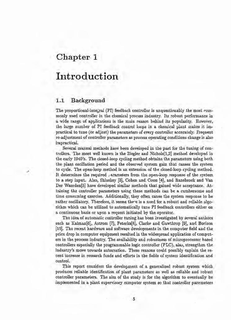
This report considers the development of a generalized robust system whichproduces reliable identification of plant parameters as well as reliable and robustcontroller parameters. The aim of' the study is for the algorithm to eventually heimplemented in a plant supervisory computer system so that controller parameters
5

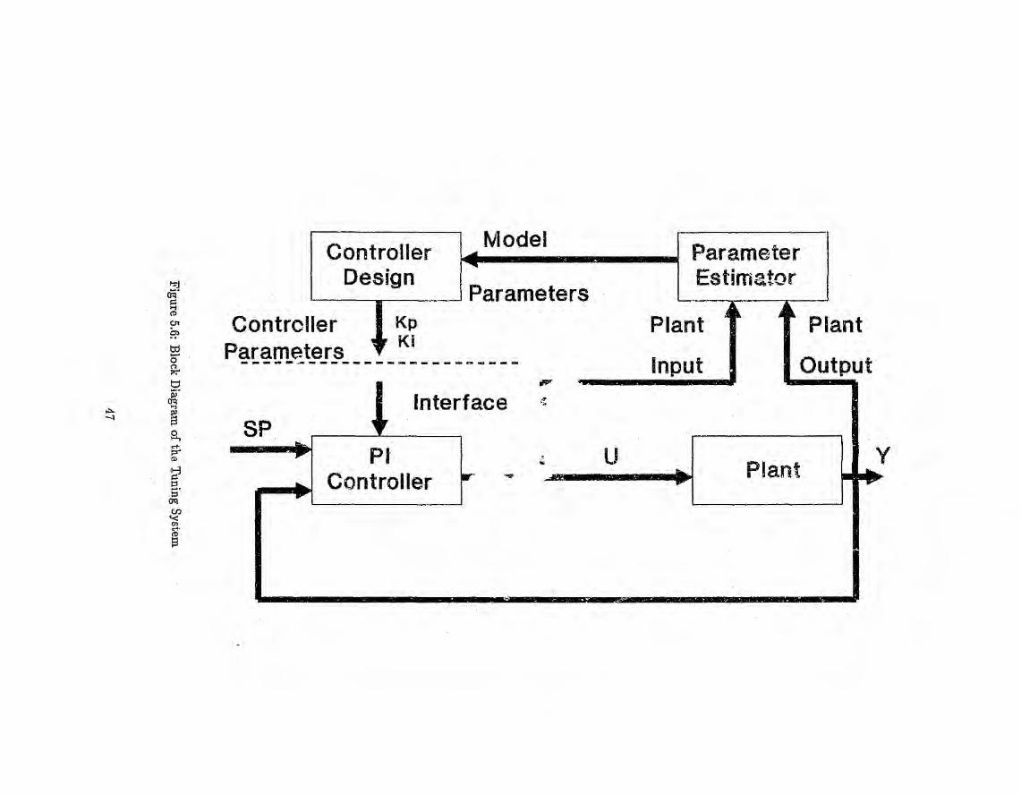
can be automa.tically down-loaded into the programmable logic controllers (PLGs)which perform the front-end PI feedback control. The concept is illustrated inFigure 1.1.
1
~',I~:".. .:'.' I. ,
-'. .• ,J
";' ·h_"",",_:._,""", ':'__ .~_~_J ~._...,..,..",.._~ .. ...,."-"'...:---,,--- .. '-' :_---.; ......';.: ""_~--- ... ~,.
.za,·OJ
>,j(1)
I-'
:fr-t
I.'.~:'" .;..:
.::;, :.I:'~'.~, "
1
1,I
:1•t
.~.
Output

1.2 Objective and Overview of the Report
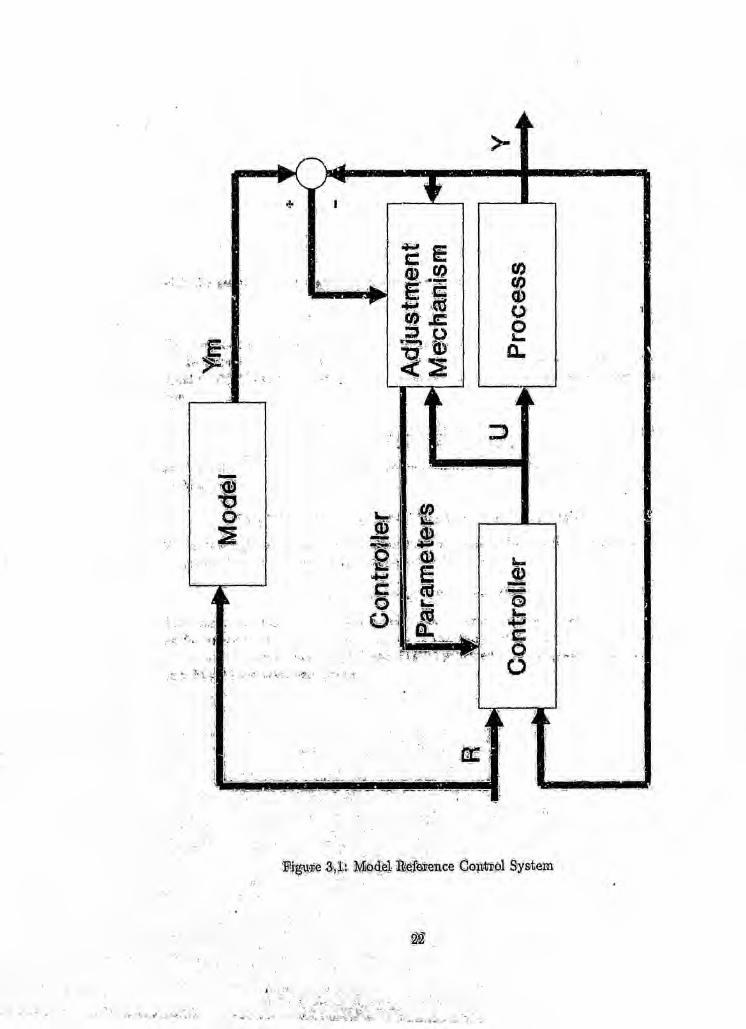
1.2.1 Objective of the ResearchThe objective of the research is to design a system that can be used to performautomatic controller 'tuning. The approach consists of a recursive parameter ~,sti·tllati'on algorithm and a controller design algorithm. The controller design algorithm.isbased on the closed-loop pole assignment method and when the process is modeledby a first-order system, the pole assignment approximates tl~~ standard PI feedbackcontroller. The method. diffees from others because the overall design is formulatedusing the delta-operator.
Some of the design's basic characteristics are the following.
s 'I'he delta-operator and its associated tr~.n',;fQ..tal.
• Signal conditioning for. proper conditioning tlf the measured signals to improvethe estimator pe1"fbrmance.
• A generalized pH)CeSSmodel that includes. both measured and unmeasureddistur bances.
e A rule-based mechanlsm fo./.establishing the location of the closed-loop poles.
1.2.2 Overview of the ReportThe r(!port is organized in the following way.
• ChapteJ.' 2 disc1l:lc<t,~Scurrent technil!~le~s used for estimating unknown parame-ters. of deternllnis.t1C syster;;.:;;s.
• Chapter 3 di:SCl'!.SS<:S. k'.'>memodern methods for designing controllers for thecontrol of linear deterministic systems,
• Chapter 4 examines the concept of the new shift-operator namely .the delta-opera·tor •.It, also, shows how the delta-operator can be related to the standardc(mtinuous and discrete time operators.
~ Ch.ap:ter.5 presents the structures of the parameter estimator algorithm and thepole assignment al,gorit}u:nused for the design ofthe controller para-meters. It,<l[SO'1 pMsents the method for formulating the pole assignment to approximate.a. S'ta:ndatd Pl1oportional.integral controller.
• Cnl:tpter 6 discusses some implementation aspects of the design such as signalco1td.1tiolling '~ndrobustness. It, also, y;reseIllts the methods of tran.slating theperfdrJ:n;mG~.iIeqm:n~mentsinto the desired lecation for the closed-loop poles.
• Oll!ap~el"7 pne$ents the ptoperties of the algorithm using simulation and realp.1~'nt1Icsts.
• C~a.ptel' S Cltln;~l)ldes tIle rEl;PQrtand p:rese1lts the main findings and recommen-d!atiions of the S·t;fi.d;y.
t 4PP~~f4xAptes~~ts tile~jer~an U-D covariance factorization method whichis me,d:i'Jiedto .i,n:c1udet1re deQ;dz0n:eand forgetting factors,.
8

• Appendix B pl'esents ... '. .\lternative method for expressing a PI controller in a.delta-operator format .
• AppeIldixC presents the method of approximating a. pole placement controllerto a PID controller.
.\
c.....,ha..P'.'tar 2x,:,_.·,'", "",.>. , '"
':g~~~~~1?lIet .,gi'ves a.t>Hefde.sctipti'on' of.s'dtite curreat approaches to. pal'arneter estl-. ~~'itto~;4'1150.;. tll!~ Q'h$iJ])\t.~f,pxese~ts ane o.f :the. t~pical <li·fi'exence ei:fuation formulas~t' .'.. '. .' " i~~te~s:;ap~l)cess l'JlodeJ. ... ' .\ :'. . . ~"~V~it~.iti~fUfie11il\('.fced;'ure·tIset! to deduce the \tal u.e$ of an l\nl'1lown.~~~~ent"b#Q$:$etvifflFJ~lT~li'futU1'7Gf( the rel!Pdzys~of the system under appropriate and·co.ll~~(':Re'(lQoil.<llirIQns.A..sUTv.ey I)f pata;metei' ~sthnatio.n methode for linear systems~;~~~.Q~s~~$>'iea sigll?Jls is given by Yo.ung [11].
.C ~:P~:¥~m~t.e~~~~i'n,:l.:~~j,,'¥ns9p.eliQ'es.CaJ). be. separated into two. general categories:~!ii"', ',"< '.' ·'H' ..'_· "'_"'.',~'. ,,"" ',,,. ';-""." -- '-,",' -, ,:'" '.,'-'-" _'" '," ,." ,>
.-
~";'i:"0af J~rh~e~ls'lilf~~~s1;,( :~(:',"~;
·O:U'·.Jil11:e.~lgoJ~itblmsis tIl-at tll(l off-line algo-;l'tr~M~~~irj'~l~t lp,P\1t ~nd. ()ut,put da.ta
prevIously on storage facilities~,!td(jllleal~~SiaJ~j~potlc'al.The en~l;j.Ile~gQtithms estimate the model parameters byGPnttn~0~sl\Y p,toce:ssb.tg h·is$orica.l a.l1d curte,pt process data .
.,@;.vi;l1J~M~h,nj~qe~'~re;mostlypreferlled by the researchers because they formt~:£il)r::~lre:f0:i:ll!lulatri(!)1lof aa~p:th,te (tQntrol philosophy. Fhlaliy, among all the,~~~1i!:);~§;~c.~he ren:u.:tsiw~least sql\l~re$ is the mo.st wi,dely used method due to.':g~fJ:~~$'..~'&t.•.tJ,~~t>;iiHty.

2.2 Linear Paramerric Process ModelA process model format which can be used for parameter estimation purposes is theIl~tel'minlsticAI};tol'egressive 'Moving Averages (DARMA) Model given by:
y{k)+d.l y(k-l)+·. '4-an Y(k "7n) = bo u(k-d)+b1 u(k-d-l)+.· ·+bm u(k-d-m)(2.1)
where: k :: '* = 0,1,2, ... is die discrete time, T; is the sampling time, .d is thetime delCliY,y and 'It are th.e plaJtlt output and i~put, respectively, and n and m givethe order of the mode].
#;$itg*h~'ba,c~wa;rd ~llIft opeta,toF, the model can b(J represented by:~-_ :,. -.-'"_ -. _." ...•, ".._ - .-~,_-- .,. - -.~
(2.2)
wh.ere:A(q~l) == 1+al g-l + a2,q~2 + + an g~n
B{q'-l) = (bo + hI«:+ b2.q-2 + + bm«:)q-dTh'a DARMA Model can, also, lyeexpressed as:
y{k):.: ,p(l. - 1) 8(k - 1) (2.3)
l.vher(J:ll(ky:rs'tne system. output a~timekq>('k...., 1) is the system's output and input history vector(I{k - 1) is the pai.'a.rnete-r v~ctOi'
The model palrameters are the unknown factors and need to be identified. Theabove niodel farms the basis for the parameter estimation schemes and it is partie-ularlr c<:lnv~nientfQr tlte s'l1hseqll:eritdevelo,p!ment of the autotunlng a1gf'rlthrn.
11
2.3 Projection Algorithms
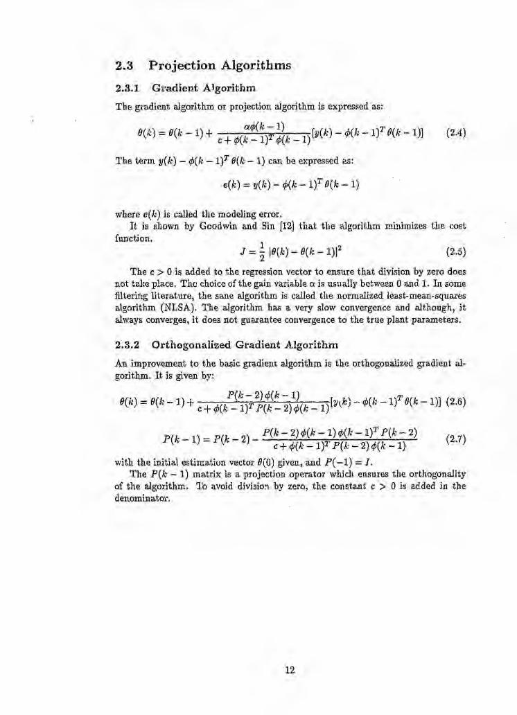
2.3.1 Gradient AlgorithmThe gradient algorithm or projection algorithm is expressed as:
lX¢(k ~ 1) .. TB(-/:)= O(k -1) + c +¢(k _l)T rp(k _l)[y(k) - ¢(k - 1) (J(k - 1)] (2.4)
The term y(k) - 4>(k - I)T O(k -1) can be expressed as:
e(k) = y(k) - 4>(k - If B(k - 1)
where e(k) is called the modeling error.It is shown by Goodwin and Sin [12) that the algorithm minimizes the cost
function.1
J ::: - IO(k) ~ O(k - 1)122 (2.5)
The c > 0 is added to the regression vector to ensure that division by zero doesnot take place. The choiceof the gain variable a: is usually between 0 and 1. In somefdtering literature, the sane algorithm is called the normalized least-mean-squaresalgorithm (NLSA). The algorithm has a very slow convergence and although, italways converges, it does not guarantee convergence to the true plant parameters.
2.3.2 Orthogcnalized Gradient AlgorithmAn improvement to the basic gradient algorithm is the orthogonalized gradient al-gorithm. It is given by:
P(k - 2)4>(l; - 1) . \. .. TO(k)::: O(k -1) + c+ 4>(k _l)T P(k _ 2)4>(k-1)[y,k;- 4>(k -1) 8(k -1)] (2.6)
P(k -1) .:::P(k _ 2)_ P(k - 2)4>(k - 1)4>(1:-ll P{k - 2) (2.7)c+ 4>(k - l)T P(k - 2) 4>(k -1)
with the initial estimation vector 0(0) given, and P( -1) = I.The P(k - 1) matrix is a projection operator which ensures the orthogonality
of the algorithm. 1'0 avoid divisioa by zero, the constant c > 0 is added in thedenominator.
12
2.4 Least Squares Algorithm
It is by far the most popular algorithm and as Goodwin and Sin [13}show is basedon the minimization of the quadratic cost function
IN(O) = ~.-£(y(k) - <f;(k- II()/+ ~(O - O(O»T Fb'l(O - 0(0» (2.8)k=-'!
The algorithm is written as follows:
P(k-2)cf>(k-l) ... . . T (B(k)=O(k-l)+ l+<f;(k-l)T P(k..;.2)<f;(k.;_1)fy(k)-<f;(k-l) e k-l») (2.9)
P(k _ 1) = P(k _ 2) _ P(k - 2)<f;(k -l)<f;(k - l?P(k - 2) (2.10)1+ <f;(k_1)T P(k - 2)cf>(k- 1)
with 8(0) given and PC-I) any positive definite matrix Po.The least squares algorithm is almost identical to the orthogonalized projection
algorithm. The covariance matrix P is an indication of the parameter convergenceand a measure the estimation error e(kJ. Usually the Po diagonal coefficient in Pis a large number due to the poor confidence in the starting parameter vector 0(0).Only when 8(0) is a reliable estimate is Po given smaller values to enable fasterconvergence.
The algorithm is a fast convergingone initially, but, when the P matrix diagonalelements begin to get smezler due to the convergence of the estimates, the algorithmbecomes more and more insensitive. Remedies that deal with the problem, modifythe covariance matrix to sustain the agility of the algorithm. Some variations to theoriginal least square algorithm that deal with the algorithm "falling asleep"(14) andwith estimation in the presence of bounded noise are presented next.
2.4.1 Least Squares with Covar-ianceResetting
This schemeis based on the resetting of the covariancematrix P at various intervals.During the time intervals k1,k2,k3, ...• the covariance matrix is reset to:
(2.11)where Ni.is a constant ranging between 0 < Ni < 00. Otherwise, the normal leastsquares update is used.
2.4.2 Least Squares with Exponential Data Weighting
The least squares algorithm can be modified by enabling memory to purge itself fromredundant data. The weighted least squares method achieves that by minimizingthe weighted cost function.
NJ:::: l:).N-k le(k)f
k=l(2.12)
where:
e(k) :;::y(k} - cf>(k~ IJTiJ(k)
13
and the forgetting factor A is a constant ranging between 0 and 1.The modified algorithm appears as:
P(k - 2) cfJ(k -1)O(k) = O(k -1) + AU: _ 1)+ cfJ(k _l)T P(k _ 2)cfJ(k -1) .e(k} (2.13)
1 [. P(k - 2) cfJ(k - 1) q;(k - I)TP(k - 2) ]P(k - 1) = "5.(k -1) P(k - 2) - >'(k _ 1)+ cfJ(k ~ l)T PCk _ 2)cfJ(k _ 1). (2.14)
For most cases, Isermann [15) states that the range. of the forgetting factor isbetween 0.95 s X$ 0.995.
The number of historical samples N that are significant to the estimate of theparameters can be aTproximated by:
1N ~ -..._..-I-A (2.15)
The performance of the algorithm improves according to Soderstrom, Ljung, andGustaveson [16J due to the increase in the weight.
XCk) = AoX(k - 1)+ (1- Xo) (2.16)
Which combined with XN-k gives
XCk) = XoX(k -1) + >'(1- >'0) (2.17)
with >'0 < 1 and >.(0) < 1-The time dependent forgetting factor discards data during initial estimation at
time increments. When >. reaches unity, the normal recursive least squares algo-rithms emerges.
'2.4.3 Least Squares with Deadzone
The robustness of the least squares algorithm when operating in the presence ofbounded noise can be improved with the use of a deadzone in the parameter updateequation. Additionally, the introduction of deadzone in the algorithm helps to con-trol "bursting", where due to lack of persistent excitation the gain increases quicklyresulting in erroneous parameter estimates.
A recursive least squares algorithm with dead zone is defined as:
a.(k-l)P(k-2)cfJ(k-1)..[ A]O(k) = 8(k -1) + 1+ a.(k -l),/>(k _ l)T P(k _ 2)¢(k _ 1) y(k) - y(k) (2.18)
where:ii(k) = ¢(k -ll O(k - 1)
is the estimated plant output and
P(k -1) :::;P(k ....2) _ a(k - 1)P(k - 2)cfJU.-1) cfJ(k - If P(k - 2) (2.19)1+ a(k - 1) cfJ(k .... l)T P(k - 2) cfJ(k - 1)
with the initial parameter vector 0(0) given and PC-I) any positive definite matrixPo.
14

The factor a( k - 1) is defined as:
{
1 'f ... e(k)2. . A 2 0, 1 .1+if>(k-l.FP(k-2)t/>(k-l) > u > ;a(k -1) =
0, otherwise,where:
~ is a constant error limit and
e(k) = y(k) - tiCk)is the estimation error,
15

2.5 Summary
In this chapter, a number of on-line parameter estimation techniques have been de-scribed. The formulation of all the algorithms was based on the DARMA m.odel.Although the methods were presented for deterministic systems, they also producegood results when used for stochastic estimation purposes. The recursive leastsquares algorithm being the most commonly used one Was presented in more de-tail. Also, presented were some important modifications to the basic least squareswhich improve its performance and robustness for specific problem areas.
16•
Chapter 3
Control Principles
3.1 IntroductionThe chapter presents Some current control design strategies based on discrete-timetheory. In general terms, the techniques can he separated into two main categories,The first is the minimum prediction error controller category. The second is theclosed-loop pole assignment category.
The minimum prediction error method designs controllers which generate an.output at the present instant of time which forces the future output of the systemto obtaln some predefined value. The dose-loop pole assignment method assigns theclosed-loop poles to some desired locations trying to accommodate some predefineddesign specifications.
The control schemes discussed here address the linear deterministic systems case.
17
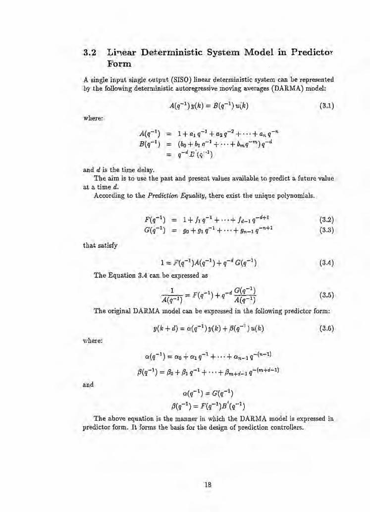
3.2 Linear Deterministic System. Model in PredictorForm
A single input single output (8I80) linear deterministic system can he representedby the following deterministic autoregressive moving averages (DARMA) model:
(3.1)
where:
A(q-l) :::: 1+alq-1+a2q-2+"'+anq-nB(q-l) :::: (bo + b1 q-l + ... + bmq-m) q-d
:::: q-d B,<;f.l)
andd is the time delay.The aim is to use the past and present values available to predict a future value
at a time d.According to the Prediction Equality, there exist the unique polynomials.
F(q-l) = 1+ h q-l + + fd-l q~d+lG(q-l) = 90 + g1 q-l + +9n-l q-n+l
(3.2)(3.3)
that satisfy
1:::: .F'(q-l )A(q-l) +q-d G(q-1)
The Equation 3.4 can be expressed as
(3.4)
1 _ FC. -1) + -d. G(q-l)A(q-l) -. q . q A(q-l) (3.5)
The original DARMA model can he expressed in the {allowing predictor form:
y(k + d) = a(q-1 )y(k) + f3(q-~")u(h) (3.6)
where:
( -1) + -1 + + -(n-1)ex q = 0'0 0:1q . .. ...O'n-l q
and0'(q-1)= G(q-I)
(3(q-l):::: F(q-l)B'(q-l)
The above equation is the manner in which the DARMA model is expressed inpredictor form. It forms the basis for the design of prediction controllers.
18
3.3 Minimum Prediction Error ControllersThis section discusses techniques for designing controllers based on the d-step-aheadprediction form.
3.3.1 One-Step-Ahead ControlThe one-step-ahead control algorithm forces the plant output y(k) to be equal tothe setpoint y·(k + d) in one step (in one sampling period). The controller thatmatches the y( k) to the y.{ k+ d) at time k + d has the form
P(q-l)u(k) = y"'(k + d) - a(q-l)y(k)
The dosed-loop system is expressed as
(3.7)
y(k) = y·(k) k ~ dB(q-l)U(k) = A(.;-l)y·(k)
(3.8)(3.9)
The one. step-ahead control law minimizes the quadratic cost function
J(k + d):;-:: ~le(k)122 (3.10)
with
e(k) = y(k + d) -1I"'(k + d) (3.11)
A stahility requirement is that the zeros of B(q-l), which are the poles of thedosed-loop system, are inside the unit circle. A concern when using the one-step-ahead algorithm is that it generates a large signal to drive the plant output to matchthe setpoint, which often is not desirable.
3.3, 2, Weighted One-Step-Ahead ControlThe weighted one-step-ahead control is given by
with
f3'(q-l) = q[p(q-l}:"" ,80]= P1 + fhq;"'l +...+ Pm+d-l q-(m+d-2)
The closed-loop system response is given by
P(q-l)y(k+d) = B'(q-l)y*(k+d)P(q-l)u(k) = A(q-l)y·(k + d)
(3.13)(3.14)
19
with
The control law minimizes the cost function
J(k + d) = {~(Y(k + d) - y*(k + d))2 + ~U(l~)2} (3.15)
The modification restricts the controller signal strength and assists in avoidingsystem eseillationsin between samples. When>. == 0, the algorithm reduces to thebasic ana-step. ahead algorithm,
3.3.3 Model Reference Control'I'he system again is represented by the DARMA model
(3.16)
The requirement is that the system output y(k) follows the setpoint y"'(k) gen-erated by a reference model which in term is driven by a reference input r(k).
The reference racdel is represented by
with
R(g-I) = 1+ hl q,...l + +hl q~JB(g-I) = 1 -I- el q-l + + er q-l
(3.17)(3.18)
A requirement is that the roots ofE(q-l) are inside the unit circle.The aim of the algorithm is to try and make the process output y(k) identical
to the reference model output y*(l.), so that
y(k) = y*(k)
and
(3.19)
An illustration of the control method is given in Figure 3.1. To design the con-trol law, we follow a similar approach to the one-step-ahead control. First, theE(q-l)y(k) is predtcter .and i;Len set equal be q-d H(q-1) r(k) to generate Equa-tion 3.19.
Using the generalized predkaion equality
(3.20)
and multiplying the DARMA monel by F(q-l) we extract the predictor form
(3.21)
20
with:
n(q-l) = G(q-l)(i(q-l) = F( q-l )Et( q-l)
and, also, the controller which is descoihed hy
(3.22)
The model reference control can be seen M being a generalization of the one-step-ahead control philosophy aiming at limiting the controller driving signal.
'~
,.._
< ----~".. ,
3,.4 Closee-Loo;p Pole Asslg:n.ment CG'nt:rolle'li's
Pale ~$igfiiIhent is :ta,'th.1iJ a .. e direct desi:iSnrne:th:ed. The philosophy oeldrud thejalgb!Uthm.Is flo"g~n~;' afL," ".cl.., ~~ntl"<lIIlawse.t-hat tlredosed loep. IIfs;tem b'IlSthe dresi!J.'edp.roper:ties i" ~~~Ji~·i\~'thE/tg~1ft~t~·,··,"',< ''',,',-;:,, "~:: ;
T}te system model is' des.Qriibedby a DAltMA model
;f.1(g--t)Y(k) ::::B(g--l)1.l{k)';P4;E't:gene~ail {~(l~1;)M~"sli;~Gtllr~}s'\gi;'Yen'b,y
(3.23)
(.3.24)
(a:.~~)b~ ~J~P~~'l¥tijl~'!~~$~l~ReUllo.$aitli'l3,fy t'~re-.
lIT ~t1fh wj~!lp.l'@'du:ae)
,~.
~ ....
f
-·Plant

3.5 SummaryThis chapter presented some controller design techniques for linear deterministicsystems. Also, examined were some areas for which the described algorithm could bea;ppIied. It is clear tha.t using the control schemes is not a straightforward procedure,~'l1ld~t~~~tio~ fIT~st be given to the constraints that govern each case. The pole~1<tGem:emt1'$t'he most preferred technique of all due to its simplicity. Also, a pointtha;t sdtou4d be made is that all the techniques presented in this chapter ate specialea:s~5olthe·pole.plateznent algorithm.",,/" ',...,: -K . '.
r.
26
Chapter 4
Discrete Control UsingDelta-Operators
·4.l Introduction~,11.e9flaip'ter presents the incremental difference operator or delta-operator intro-ducecl. 'bY(jao;awin et al[18J.lt offers a number oi advantages which can be gainedhy using the delta-operator as an alternative to the discrete shift-operator,
The delta-operator concept is not something new. It was used in the past inapplIcations such as motivating the z-transforms, improving digital filter behav-lot, ap,ltl ;,t,o. improve finite word length characteristics regarding. controller design,J:<;)U[l;d.Qff noise ana coefficient representation as recently presented by Middletan andGQ~qwin[19].The delta-operator Call, also, be used to resolve problems that arise'froID the sa;mp:ling of continuous systems and converting continuous transfer func-ti011S t.o their discrete counterparts.
27
4.2 The Delta-OperatorThe delta operator is defined by:
q-l6 = -z;;- (4.1)
where q is the usual forward shift-operator and ti is the sampling interval.Equation 4.1 represents 6' as a Euler approximation to the derivative-operator
D == -it which as indicated by MacLeod[20] is proven by:
.0 x(t) x(k +.6.) - x(k)~
ti= q - 1a:(k)
b.= 6' x(k) (4.2)
The above relationship shows that assuming fast sampling, the derivative oper-ator can be approximated by the delta-operator for purposes of translating analogdesigns.
The delta-operator can be represented as:
6-1::;.~ ::;. b.q-lq -1 1-s:' (4.3)
TIle above formula establishes that the o-operato:t can substitute the backwardshift-operator q-l.for plant model representation. Analyzing the expression below,We have
and
(1 .....q-l)Yout(k) = .D.Q-1Uin(k) so
yout(k) - q-1Yout(k) = .6.q-1Uin.(k)
finallyYout{k) = Yout(k - 1) + AUin(k - 1) (4.4)
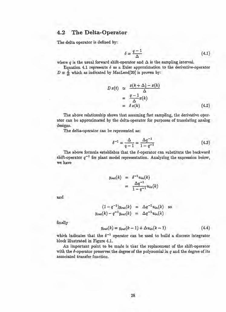
which indicates that the 6-1 operator can be used to build a discrete integratorblock illustrated in Figure 4.1.
An important point to be made is that the replacement of the shift-operatorwith the 8"opera,tor preserves the degree of the polynomial in q and the degree of itsassociated transfer function.
28
,.-I
...-." • ~~.._.....=:0>-
~
I
er~
I, I
+.""'-
+~I
<J........ A "~........
C-
Figure 4.1: 'l'he Discrete Integrator
29
4.3 The Delta..Operator Transform Domain
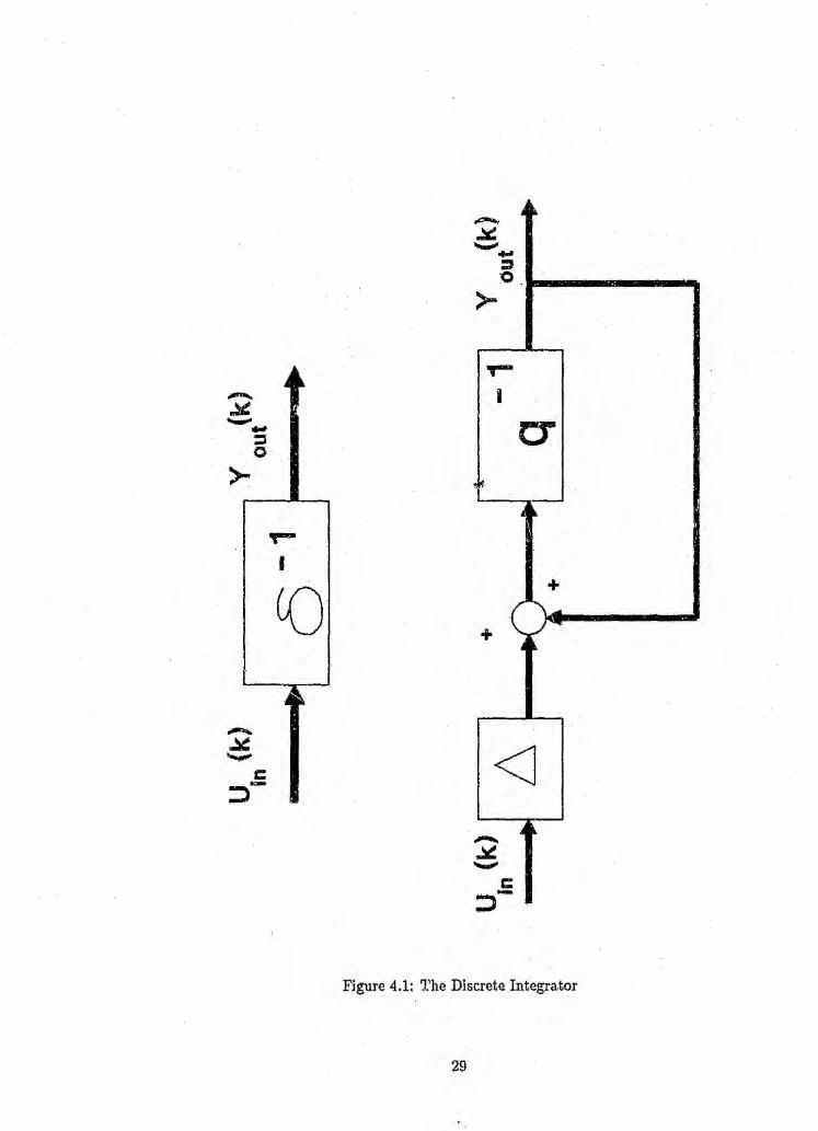
The transformation of the Cooperator is defined as the "(- transform. A distinctionbetween continuous and discrete models regarding stability is that for the former,the system poles must be in the left plane of the S domain where the later requiresthat the poles are inside the unit circle. In the "(~transform domain, this problemis overcome. The stability region of the ,-transform is the inside. of a circle withcenter -k and radius t. It is obvious that as the sampling interval decreases or thesampling rate increases, the stability region increases and approaches the continuousstability region as illustrated in Figure 4.2.
The definition of the ,-transform is given by:
co
F..,(i) = AFz(l + 6"() == A Ef(kA)(l + 6,)-ki=O
(4.5)
where Fz is the z-transform and z is replaced by 1 + A"( and it represents thetransform of the e-opera,tor models where q = 1+ 6e.
It has been proven that the ,-transform converges to the s-transform as thesampling rate increases. This is shown by:
lim {F..,(/)} = Psls=.., == (>0 f(t)e-..,tdt~_O h
where the integral is a Riemann integral.The standard formula for replacing a ~ model with a .6-model is:
(4.6)
ACe) = ~n A'(Ab + 1) (4.7)
where:A' = A(q) == qn + an..;.lqn-l+ ... + ao
and n the order of the polynomial A( q).
30
Gamma Plane
-1/6
Figure 4.2; Stability Region of the '1-Transform
31

4.4 SummaryThis chapter described the a-operator and its associated I-transform It discussed theprinciples behind the a-operator and the advantage it has over the shift-operator andits z-transforrn in various applications. An important issue is that the replacementofa system model expressed in a shift-operator by a-operator model does not affectthe order and relative degree of the model. Also, presented was the rapprochementbetween discrete and continuous control where the I-transform is the catalyst.
32
Chapter 5
Design of the Regulator TuningSystem
5.1 IntroductionThis chapter presents the approach followedfor the design of the robust controllertuner. The system is comprised of two parts. The first is the robust parameterestimator and the second, the controller design. Separating the system into thesetwo distinct parts results in a so-called explicit algorithm.
The recursive least squares algorithm was identified as a suitable identificationmethod for determining the process parameters. It was used for developing thestructure of the parameter identification algorithm. Modifications were performedon the basic least squares scheme to improve its performance.
The second step of the explicit algorithm is to use the parameters estimated from .the first step to determine the regulator parameters. The design method for thesecond step must he a suitable and robust method. The closed-looppole placementalgorithm described by Astrom and Wittenmark[21) has been shown to fulfill theserequirements. Due to its robustness and simplicity, the pole placement algorithmwas identified as the most suitable controller design algorithm for determining theregulator parameters.
The complete structure of the regulator tuner is formulated based on the 0-operator.
33
5.2 Parameter EstimatorThe process model given in terms of the 8-operator is described by the DARMAmodel
A( 8) y(k) = B(S) u(k) + FCS) z(k) + d(k) + €(k) (5.1)
The expression includes both deterministic distt,,:nance and random disturbance andmodeling errors.
• z( k) = measurable disturbance
• d( k) = deterministic disturbance
• e(k) = random disturbance/modeling error
The polynomial degrees ate:
dey A(8) = ndeg.13(t5) ;:: m:5n-1degF(§) = r:5n
/ Polynomials A(S), B(t), and Ji'(S) are monic described as
A( 3) = §n + (Zn-l 8n-1 + + CZl0 + aoB(e) - om + bm-1 sm-l + + bio + boF(S) :::: ST+fr_lsr-1+···+ho+fo
Inclusion of the measurable disturbance term z(k) in the model, allows the de-velopment of a feedforward model which can be used for determining Ieedforwardregulators.
The unmeasurable deterministic disturbance signal d(k} can be modeled as:
D(S)d(k) = 0 (5.2)
where D(\5) is a monic polynomial with non-repeated roots on the stability boundary.IUs a nulling polynomial since it eliminates the deterministic signal.
For a constant disturbance signal having the form
d( k + 1) == d( k )
MacLeod[22] has shown that
d(k + 1) - d(k)d(k + 1) -- d(k) ;:: 0
(q-1)d(k) = 0
It. shows that the nulling polynomial in q-operatot is
D(q) = q-1 (5.3)
and D expressed in cooperator form becomes
(5.4)
34
where:q-l
0=--·~
Along the same lines, it is shown th1\t for a sinusoidal disturbance signal
til(k) = Asin(wk k+ 4» (5.5)
the D polynomial in o-operator is
(5.6)
where:w::: l-COSWk
Operating on both sides of Equation 5.1 by D(o), the random deterministicdisturbance d(k) is eliminated. The expression becomes
ACe) D(8)!J(k) == B(S) nco) u(k) + pro) D(o) z(k) + D(o)e(k) (5.7)
Since 1)(8) has roots on the stability boundary, the noIse/error modeling term~(lc) could be amplified at high frequencies. The phenomenon can be avoided byintroducing a stable polynomial D'(S) "close" to the DCo) polynomial. .
Assuming that the dete' mlnlstic disturbance d(k) is a constant (d. c. offset dis-turbance) then the nulling polynomialls
DCS) = 0
The stable polynomial, n'(S), then is
D'(o)=o+e (5.8)
where e is some small positive number.The function if, removes the deterministic disturbance and does not distort the
spectrum. It is obvious that tile function 1ft is a high- ....1SS filter. By approximating8 ::::! jw, the filter has the frequency transfer function
D(jw) jwD'(jw) = jw + t (5.9)
with corner frequency the small number s.To avoid having high frequencies present which are above the Nyquist frequency,
alow-pass filter is also introduced. It ensures that {.Iteband limited model is excitedonly by frequencies which ate necessary to give a good process model. The structureof the filter is described in the next chapter.
The "filtered model" is described by
(5.10)
where YJ, Uh kf, nJ are the filtered process measurements,The DARMA model can be represented in the regression format:
en VI(k) ::: rjJ(k - l)'I'O(k) + nf(k) (5.11)
35
where
4>T ::: [ct1-ly/(k), ... y{(.k),cm uJ(k} •. · uf(k), 81·~f(k)· .. zJ(k)] (5.12)Ii ::: [-an-1,'" - ao,bm1• .. bodr'''' fo] (5.13)
This is compatible with the recursive least squares algorithm described in Chap-ter 2.
To enhance the robustness of the estimator, the algorithm was modified to in-clude both the deadzone a(k} and exponential weight >'(k) factors,
The modified recursive least squares algorithm expressed in t5.operator format isgiven below.
... .' '. '. .. . P(k -2)4>(k -1) .." .e(h)::: fJ(k - 1}+ ark - 1). >'(k -1) + ¢(k -1)T P(k _ 2)4>(k"";1).e(k) (5.14)
......' 1 .. [., " P(k-2)4>(k-1)¢(k-1)TP(k-2) 1P(k ....1)= >.(k _ 1) P(k - 2) - a(k -1) ...\(k -1) + ¢(k -1)1' P(k..:, 2)¢(k - 1)]
(5.1.5)with
e(k) :=. Yf(k) - ru(k) (5.16)
with flJCk) the estimate'd plant output.Finally, to improve the numerical sensitivity of the algorithm the Bie;rman[23]
UDr;T factorization technique is used. The technique is presented in Appendix Amodified to include the deadzone and exponential forgetting factors.

5.3 Controller DesignThe design of the contrQUer emerges from the use of the P ~.~placement algorithmdescribed in Cha.pter Two and the application of the internal model principle. Thecommon error driven control system including a.n output disturbance d(k), as Illus-ti:'ate~l j,n FigUre 5.1, is the principal hlock diagt<llltl.the design is based on.
TIre setpoint y"'(k) is defined as a sequence that can be generated through aIinear finite dimensional system described by
S(8)y"'(k) = 0 (5.17)
where S(8) is a monic polynqrnial with its roots lying on the stability boundary.The nulling polynomial, D(c), is used to negate the output disturbanc~l d(k), as
it was desr.:r.ibedin th.e previQus section.The feedback control law 'used in developing the design is given by
L(8)u(k) ~ !/Il(8)ll"(k) - P(c)y(k) (5.18)
where
1.(8) ::$. 0" + 171' .. 1811--1 + ... +h 8+ 10~-:I•. · .,
J>(8) ;:;; 8P + Pp--l 8P--1 + ... + Pl 8+Po
Applylng the Inuernal M~del Ptinciple[241, we assign
11'1(8) = P( 8)L'(e) == L(8)D(o) S(c)
thus modifying the contrpller poles to inotude the reference model poles S(8) andthe distm'bance poles .o(8}•.Tlle control law becomes
L(8)}).(8) S(~)'lt{k)#: P(o) [y*(k) ~ y(k)] (5.19)
I;'(8)v/(k) ::::P(6) e(k) (5.20)"<.;/'
'\Viherae(k} ::::;rl·(~i~:,YKk}t~~he£eed\b.ad: error slgnal.!tn.. a tl9:t. sfl!niq1ft~~:~9'wn... .. IDod:Uied clQs.ed-loop H1ustl'ated in Fig~re 5.2 can
b.;e ;E~ltie$\)niPe.Q: !b"y ',tlie irll;l:n:s ;tVitrot1'Qn \l:;.' _, - - -: ': - - -~ ., - '. - -,~ - .._ '_ - - :
(5.21)
(5.;2.2)
y(k)
5.3.1; , Oont.l1a:HerD'esi.gJil for First-Orde,r Plant
A wide rron;ge.of ch:~fi:i!i~alj,)j;.ocess p1<lints..can a4equa.tely he modeled by first-orderm(jd~l$. When the pole placement algorithm developed previously is worked outbase'd on a. fill's,t"0-l'de.r.illlodel, the atgorNllul1 develops as follows.
The control law .is represented by
L'(8)u{k)::: P(5)e(k)
or .bl;·:~:·¥r8insf~rfU'ltctfon farmat
u(~) __ ....... p ."",.'.peek:,' .,...Gs - tl:- 'L,DS
(5.23)
(5.24)
fl.)I~~.pTbGessis lle.p:resented as.:a,fhst-order model given by the linear deterministice!l~a:~ijj1;'( .
(5.25)'!l'ijt~)al~t~t.nlmi's.tlcd:i'S.t\ttban!c~isaSsumed to he acansi,a:nt d.c, offset disturbance
!1j~ M -. -; ,- , J)~iYi).~fW~,a;l. " .." ,
19(8);:;: 8
,$ ::= 1
kj~ep;enaJl ru;Ie for d<'Thning the a.egree of the controller polynomials Land P is
',1ilL~d:Me~L.', == (}:e!J;r~e.,4,,,,,, 1d~:g.r~eP Q degree A + deg1'ee D + degree S ~ 1
4'&g,1'eeL == @
d'etliree P = 1
wlulGh; \I1~§,'U1;ts t~~p.i:l¥qementeOIl\1i!101law
(5.26)
~~Pt1iii~1l'~~(~gn:Qul1i'Iia,hp:rls> the n)~'l3!LI!;~!l'('il;ynomi.aft 1)( c). It is~iW~l,~~i~l\igf~:~~H:;bill)J!(;l,*l>,;~~~:g~p:¢t:aJ~~~~h~httegral t¢'l'01 in the
'::''(',:.\. ':\'.~- '. .
(5.27)
'~~'I4~:fp";*'tl~~Ytefts - '1~§!~;MlYa
(5.28)
(5.29)
'2 ',"" ", ",' , " 2, * '*108 + ao/o/S +P1boo +Pobo == 8' +a18+ ao
:it3~I[tta~ingc(J{!':ffi:cientson e!<tlte.rsi{ie of Equation 5.30 results
(5.30)
"f 10 'J' ,[" 1 1M:a.,. P,l =,., a[ ,.Lpo, "ao
~~B··.~·!~jij4\fi:~M6ri§;,3@ 'c~n b~ soPvea ,s,eq!!i'eIl.tially 'for 10,Pl, Po by",:.,:"":",, ';;,:, -: 'j
M -- 1 (5.31))t itt - aop~; _':!1-
1)"(5.32)
0aj"I.
(5.33)Po ",0,
tie, ,"~h:g\llext $],ep isto correlate the pole placement coefficients with those of a PI
l'egU)}i;Mloj)'. '
5.4 Approximation to a PI Regulator'lPhe ideal analog PI controller is given by
u(t) = tc, [eft) + i; J e(t)dt] (5.34)
where JIrp is '6h'eproportional gain andZ] is the integral or reset time.Equati.on 5.34 written in the Laplace domain becomes
U(s) = l{p{l + is)E(8) (5.35)
(5.36)
where ires) and E(s) are the Laplace transforms of the controller output and errorsignal" te$pectively and l(i is the integral or reset gain and K; = :A.
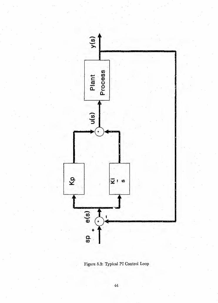
A typical cascade PI closed-loop is illustrated in Figure 5.3.The ;PI regulator operates on the actuating signal and produces Cine that is
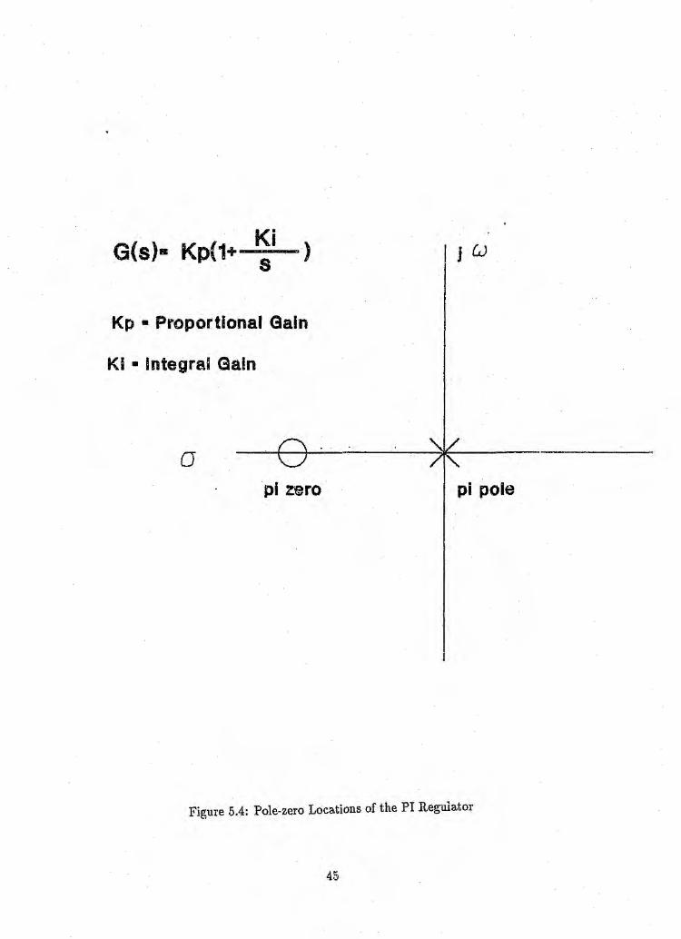
proportional to both the magnitude and the integral of this signal. TI'e integralpairt continues to Increase aJS long as an error signal is present. The locations of thepole and zero of the regulator are illustrated ill Figure 5.4.
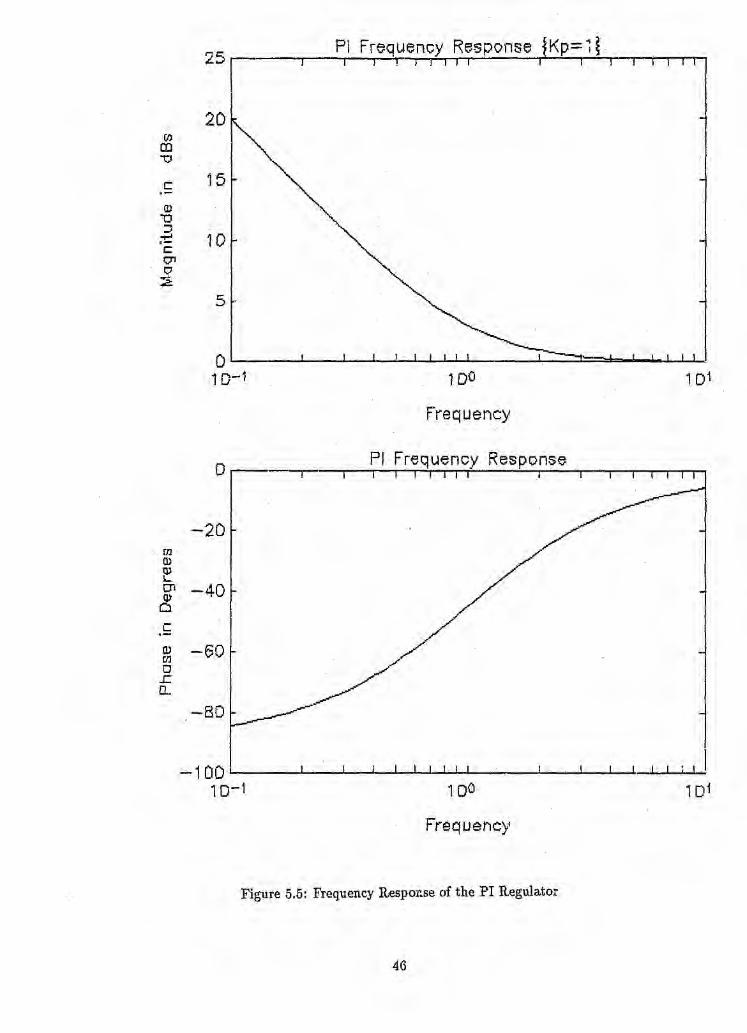
Examining the PI controller in the frequency domain, it becomes obvious thatthe regulator has a phase lag frequency response as illustrated in Figure 5.5.
At low frequencies the regulator amplifies the system gain thus reducing thesystem sensitivity., It reduces the steady state error and improves the stability ofthe lQop.
The Equation 5.36 can be rearranged to:
Us = Gpl(S):::: Kps +J(pKiEs S
(5.37)
Using; the app.roxlroa;tfon .s :::: {; (assuming fast sampling), the equation becomes
GP1(8) = '{pc ~ [(pKi
Ccilll'l>a:dng.Equation 5.38 with Equation 5.26, we have:
(5.38)
GpJ(C) = Ce(o)
(5.39)
i~t·\isQ~'vious th~t the. Goeffl!:ieltts of the two control laws correspond to eachGtlter. ri['iie :fhll(>w,i\~g..r.e1aitiol'1is,htipsex,lst:
[,(p - PI__ poI<i .PI
(5.40)
(5.41)0r
(5.42)

The proportional and integral gain tan be determined by the Pl and PO coeffi-cients. Figure 5.6 illustrates the general block diagram for the generation of the PIparameter.
Another method of approximating the pole placement controller to a PI controllercan be seen in Appendix B.
It isapparent that we can use pole placement techniques to tune the PI controller.It is, also, apparent that the closed loop polynomial A" is of great importance to thealgorithm. Correct selection of A" is essential. The A" can be generated based on thetime and frequency design requirements, i.e, damping ratio, phase margin, etc. Theselection of a suitable A 1ft is given in the next chapter. . litionally, Appendix Cpresents the formulation of the pole placement for a second-order model and itsapproximation to a PID controller.
4.3
.-... A ..
(/).........~
U)..... enc (I)ctI 0- 0a.. f_
o,
~ it.
.-..fJ)-:J... .....
0. .-~ ~ I 0
~ j to
r,.- 6'·(f)~Q)
+ .t ..C.en
Figure 5.3: Typical PI Control Loop
44
KiG(s)a Kp{1+ s )
Kp .. Proportional Gain
KI • Integral Gain
j CJ
opi zero
Figure 5.4: Pole-zero Locations of the PI Regulator
pi pole
-20rnmE01 -40IJ)
C!c ./.-m ---60[Il
0..c0..
-80
~10D . I I,
10-t 100 101
Frequency
f/JCO"'0
c 15.-CD"'0:J~ 10cO'l1;7:2
2D
PI Frequency Responsej j ! I I j j I
5
1 DO
Frequency
o
Figure 5.5: Frequency Response of the PI Regulator
46
Model...._ControllerDesign
'--~ ~----l Parameters
ParameterEstimator
Plant J ~ ~ ~ Plant
Input Output
Controller KpParameters ' , Ki------------------~~-----SP " ,~""~
".. PI ..Controller ~ "OJ'
III....
Interface
Plantu y

5.5 SummaryThis chapter has presented the design philosophy that forms the basis for the con-troller tuning system. The algorithm was constructed using the 8-operator.
The estimator agrees with the recursive least squares method modified to handlecovariance resetting and bounded noise. The controller was designed utilizing thepole placement and the internal model principle. The controller coefficients arefound solving the Diophantine Equation. The inclusion of the disturbance nullingpolynomial generated an integral part in the control law and solving;the controllaw for a first-order plant model enabled the approximation of the pole placementcontroller to a PI controller, l.180, some discussion was made on the importance ofselecting a suitable closed loop polynomial A*.
48
Chapter 6
Implementation Aspects
6.1 IntroductionThe chapter discusses some practical' Issues that can influence the implementation01 the estimator and controller algor;UnTI s, More specifically issues such as thechoice of the sampling rate, signal cond.tloning, and selection of the correct startupparameters Le, dead zone and forgetting factot, come under examination.
The performance of the estimator is heavily dependent on the Implementation ofappropriate filtering techniques. Filtering i" necessary to enable the removal of highfrequency noise, and d.c, values which can Jnfluence tllC ablllty of the estimator toconverge to the real parameter values.
A very important issue in achieving optimum performance of the system is theselection of the closed-loop polynomial A". The A" is established using a set of rulesthat convert the design specifications to a set of dosed-loop pole locations ..·
49
6.2 Sample Rate SelectionThe selection of the best sample rate for a dig-ita! control system depends on manyfactors. The absolute lower limi,t to the sample Irate is based on the SaItlplil'6 the-orem. The sampling theorem states that to reconstruct a band limited signal fromsamples of that signal, one must sample at twice the rate of the highest frequencycontained. i,n the si,gn;al.Ths theorem can be expressed as:
(6.1)
where:
Ie is the sampling frequencyJb is the plant bandwidth
Quite often in practice, the Nyquist criterion given by Equation 6.1, can beinsufficient in terms, of system responses and system sensitivity thus, the need tosample faster arises. Franklin and Powell[251state that faster sampling reducesdela~'between input change and system response and smoothes the system outputresponse applied to a plant through a zero-order hold. Also, Goodwin and Sin[26]recommend that the sampling period be an even multiple of the time delay whenthe plant delay is a priori.
50
6.3 Signal Conditioning
This section describes the design method of the high-pass filter (hpf') and low-passfilter (lpf] which are implemented for proper conditioning of the measurement sig-nals.
6.3.1 The Low-Pass FilterThe filter is implemented so that the noise above filter breakpoint is attenuated.A design requirement is to select the filter cutoff frequency, We, in such a, wayas to encompass the plant bandwidth. Another requirement is to provide enoughsignal attenuation so that the noise when aliased does not affect the estimatorsperformance. The two requirements tan be formulated as:
1we ~ '2ws
We == 1Wb
(6.2)
(6.3)
where:
Ws ii the sampling frequencyWb is the plant bandwidthWe is the lpf cutoff frequency
The discrete filter implemented in the algorithm is the realization of an analogfilter with the transfer function.
~HI (8) __ Wr
PJ - 82 + 2as +w;The magillitude 'of the filter is given by:
(6.4)
W2A(w)== r ..V( 10; - 'UP? + 4a2w
The d. c. magnitude of the filter is:
(6.5)
which is a ~onst:Q.int that, if not satisfied, could as stated by Bergensen[27] render111reintetnal es't~matClrV3:tla,);llesnumerically sensitive to finite-word length errors.
Setting the real paxt 11. of the filter's complex roots equal to imaginary part b,the 'fitter Is testl''i'<;tea to -'1. no-overshoot resp<1n$e.
T4e magnltude of the filter at the cutoff frequency hl:
andWo ;:: Wr
51
The analog filter has the following characteristics.
=/3 Wea = J2We _- Wr
(6.6)
(6.7)
The discrete filter is constructed using the bilinear transfermatlon,
(6.8)
thus we haveW9(8) _ .. .. . r ..
. - 82 + 2as +w~which re$tl!litlSthe discrete low pass filter
(6.9)
(6.10)
where:
It'!}1 = w2']."2r
p,v2 = 4aT
ande2 = 4p,v2 + p,v!Cl = 2p,vl- 8!C2eo = 4.,_ #v2 + P,VJ!e2
72 ~ P,?)!!e271 = Zp,vl! C2
70 = p,vl!e2A block diagram of the dlscrete low-pass filter is illustrat¢d in Figure 6.1. Also,
illustrated in }rig,ute 6.2 ana Figure 6.3 are the frequen~y responses of both theanalog and digital filt~TI'. Tll(~~repetition of the digital filt~r response is due .hefact. thatthe filter mi; ,shltud~ ahap'n~e are periodic functioIls ofw with perk fs,where is is the Nyqli.hst frequency. To determine the resulting response, it. sumcestherefore to cOli·s!1>dertIre h~11>(lNjorof the digital fiLter in the fllhdamenta.l interval( - 1'& I is)· only. ,.
~h:e c.uit.~fff1lequ,ell!ct.~f the flitter .).Sdefined by the designer during the actual(l;pplicati(!)iJ,'lZIf the alg~ti\'lil1rrn"'iFh.ei syst~m, ailsa, makes the neG~ssary checks ensuringthat tM t:~q;l,til'~llleXLtsd:i6hl1tell 'by ID!Ji~a:lllQns 6.2 and 6.3 are a.dl~er~d to.
6,,$.2 The ~ig:h..~~~~$. ~ll~~r,':,~,- '""-
In Chll1pter Five, dXIi'!.lip,l$ ~Rede:velep:Uileltt of the to:b:ust estimator the hlgh-pass filter(hpf)
@;rtpl'(o) ~- ire (6.11)
Was g~~eratecl .. The :fi1t¢f,1~1);1u:!>ed.W,fihe~atg(;jri.t'h\m te eli,rrtl>,vatethe d.c, values duringth~ parameter Ide1tt.ifiiGa1J.lollsitate.
Filter Response
DlgrtOI Low Pass Filter ~e6ponse
' -. -:-::",........
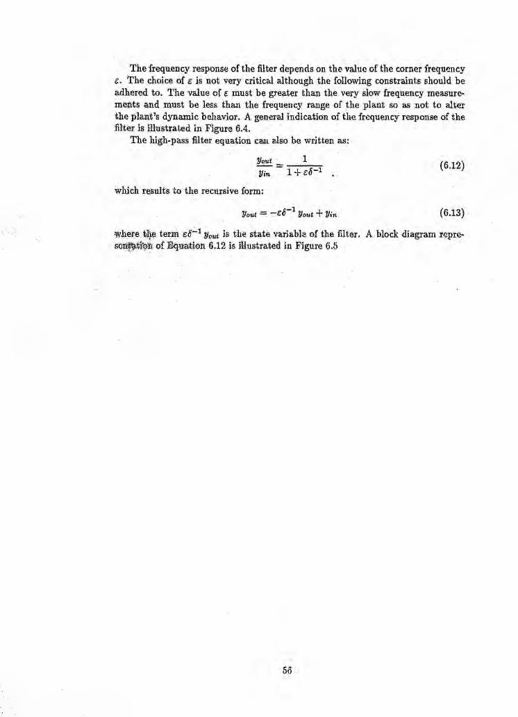
The frequency response of the filter depends on the value of the corner frequencye. The choice of e is not very critical although the following constraints should beadhered to. The value of e must be greater than the very slow frequency measure-ments ~nd must he less than the frequency range of the plant so as not to alterthe plant1s dynamic behavior. A general indication of the frequency response of thefilter is i\Uustrated in Figure 6.4.
Th~ high-pass filter equation can also he written as:
'!lout 1Yin = I+ £0-1
which te,sults tQ the recursive form:
(6.12)
(6.13)
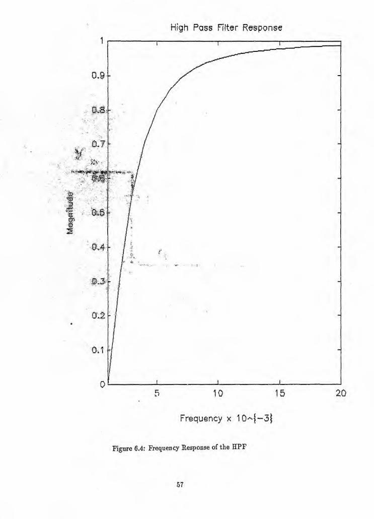
Whe;ll~v~~term £0-..1 '!I(lut is the state variable of the filter. A block diagram repre-sOIil[~li~~!r,()f ID:q.urotloIl6.12 is iHllstrated in Figure 6.5
56
High Poss filter Response
Frequency x 1O,,{-3~
Fig,ute 6.4: Frequency Response of the rIPF
57
y .in
1
Q r-- ........;-oY.... out
Figure 6.5: Block Diagram of High-Pass Filter
58
6.4 Exponential Discounting and Deadzone
6.4.1 Exponential Discounting
A simple way of ensuring good parameter variation tracking is to use exponentialdiscounting to discard old data. Astrom et.al[281 have presented good practicalresults with application of the forgetting factor '\.
The choice of the forgetting factor ;\ for the parameter estima.tion depends on.thespeed with which the parameters vary, the model order, and the type of disturbancesthat are present. For constant processes or very slow varying processes ,\ = 0.99 isrecommended. For slow varying processes and stochastic disturbances, 0.85 :::;,\ :::;0.90 is an appropriate choice. The "'factor influences the memory length N of theestimator and thur the number of samples that are used by ' .. The relationshipbetween Nand ,\ is given by:
1N == ---.1-,\ (6.14)
For instance, when:,\ ~ 0.99 N::: 100.0,\ == 0.85 N == 6.666,\ == 0.90 N == 10.00
Also, effective is the application. of the variable forgetting factor
'\(k) == '\o'\(k -1) + (1- '\0) (6.15)
which imposes exponential data weighting for a transient period. Typical startingvalues for the algorithm are:
'\(0) == 0.95AO == 0.99
Included in the tuning algorithm, is the option of using the fixed or the variable ,\factor.
6.4.2 Deadzone
The lack of excitation for a long time can affect the gain PC k) of the parameterupdate equation and cause an output burst. TIle estimator performance can beenhanced and avoid an estimator wind-up with the use of the deadzone method,The aim of the deadzone is to allow the update of the parameter vector only whenthe data from the :,lant contains useful information. It achieves this by "switchingoff" the parameter update equation when the estimation error e(k) is smaller thansome specific threshold. Ega,rdt[29] and H1igglund[30] have designed very good tech-niques based on this idea. The two principal deadzone methods used to turn off theestimator are presented next.
Constant 'I'hreshold Deadzone
In this case, the deadzone threshold is a priori factor. The deadzone a( k) dependingon the comparison between the estimation error and the noise size takes the fixedvalues:
() {0 if le(k)1 s 2A',
a k == ..1.,' if le(k)1 > 2A
59

where e(k) is the error between the actual plant output y(k) and the estimatedoutput y( k). Thedeadzone simply turns off the parameter vector update when theerror e(k) ::; 2& and TJ( k) is a bounded noise sequence such that I:l. ~ 11J(k) I.
Variable Threshold Deadzone
This method implements the idea of using varying threshold, adjusting to the mag-nitude changes of the plant measurements. It is based on the reasoning that theestimation error, due to the bounded noise, is directly related to the magnitude ofthe plant data used by the estimator.
The deadzone a(k) is defined as:
a k _{ 0, jf liCk)1 < /3m(k);(.) - a» f(e(k),(3m(~~)/e(k) otherwise.
The function m(~') is given by
m(k) = crom(k ·~·1)+(l- ao)eo+ c1lu(k - 1)1 + £2Iy(k -1)1 (6.16)
The COnstants are co, ell £2 ~ 0 and aot( 0, 1).A constraint is that m(k) must be greater or equal to the bounded noise sequence
TI(k) at all time thus,m(r.) 2;: 1J(k) k2;: 0
with trIO) = moi mo 2;: O.The function (3 is defined as
with a, ~ 0 and a€(O, 1).The tuning system has been designed to allow the user the option of utilizing
either the fixed or the variable deadzone. Establishing the values for the variabledeadzone constants is a difficult process. Often the conditions the estimator operatesunder do not warrant the complexity associated with the relative dead zone thus thefixed deadzone is used.
uO
6.5 Selection of the Closed-LoopPolynomial
The behavior of the process must agree with some desired dosed-loop performancespecifications. It is necessary to appropriately choose the polynomial A* SO that thedesign specification can be achieved and translated into a set of dosed-loop polelocations.
When the process is represented by a first-order model, the closed-loop polyno-mial is given by:
A"'(o) = 62 + ail + ao (6.17)
Approximating 0 ::: S enables A·Co) to be identified with the second-ordercontinuous-time system
A*Co) = 02 + 2(wlIc + w~ (6.18)
with ( and WlI the damping ratio and natural frequency respectlvely. Correlation ofthe coefficients of the two equations results to:
a* ::: 2(WlI1
a* = w20 11
thus relating the Aoj< polynomial coefficients to the transient performance specifica-tions for the system.
The A" coefficients are generated using a set of rules[31J which are built into thealgorithm. The rules address both the time and frequency domain areas. These ateas follows.
a. Time Domain
P.O. ::: 100e-('rr/~ (6.19)
(6.20)NT(wn
where P.O. is the percent overshoot of the system, Ts is the required settling time,and NT is the number of time constants r within which the system is expected tosettle.
The user defines the P.O. and T; and the algorithm identifies the correspondingdamping ratio, (, and natural frequency, w'7' A normal range for ( is 0.450 ::; ( ::;0.7D'l.
h. Frequency domain
( = O.Ol<ppm. (6.21)
Wr = wnJl ~ 2(2 (6.22)
Mpw ::: (2(jl- (2rl (6.23)
W3db ::: wnCJ(2 + 1+ () (6.24)
'where c/>pm is the phase margin, w,. is the resonant frequency, Mpw the peak magni-tude, and Wsdb the 3db frequency. The above equations hold when ( $ 0.707. When( ::: 0 then WI' ::: Wn• With the above rules the desired system is examined forrelative stability in the frequency domain. The phase margin is established from thedamping ratio. If the resulting <Ppm does not meet the given specifications the user
61

can define the required <Ppm' The algorithm produces the closed-loop system param-eters by examining both the frequency and time domains. and enabling the user tomake the appropriate modifications if necessary. Also, the algorithm ensures thatthe bandwidth of tht: compensated system does not violate the sampling theoremconstraints by ensuring that the system bandwidth does not overbound the low-pass:filtercutoff frequency We' The rules are described in the following pseudo-code.
BEGIN
DEFINE THE PERCENT OVERSHOOT
DEFINE THE SETTLING TIME
CALCULATE THE DAMPING RATIO
CALCULATE THE PHASE MARGIN
IF PHASE MARGIN NOT WITHIN LIMITS THEN
DEFINE THE PHASE MARGIN
CALCULATE THE PERCENT OVERSHOOT
IF PERCENT OVERSHOOT NOT WITHIN LIMITS THEN
GO TO BEGIN
ENDIF
ENDIF
CALCULATE THE RESONANT FREQUENCY
CALCULATE THE PEAK MAGNITUDE
CALCULATE THE 3DB .I!'REQUENCY
IF 3DB FREQUENCY IS .GT. THAN THE LPF WC FREQUENCY THEN
GO TO BEGIN
ENbIF
62

6.6 SummaryThis chapter presented some implementation issues which axe essential for ensuringthe robustness and good performance of the ali. orithm. It formulated a methodologyfor choosing the correct sampling rate, for implementing the correct signal condi-tioning methods, and for choosing the appropriate initial parameter values such asthe deadzone and forgetting factor;
The close-loop characteristic polynomial A"' is constructed using continuous-timedesign specifications such as the damping ratio, settling time, natural frequency, andphase margin. These variables get used by set of rules that convert them to a set ofclose-loop poles that form the A"'.
I63
Chapter 7
Experimental Results
7.1 IntroductionThe design work is substantiated witb the use of simulation and teal plant tests.This chapter describes the tests that were performed to evaluate the algorithm withregard to:
a. Performance of the parameter estimator in terms of convergence, parametertracking error minimization, and data discounting.
h. Controller robustness, adherence to design specifications, closed-loop perfor-mance to reference signal changes, and system stability.
Some comparisons are made with results obtained from using the Matlab ARXestimation routine. Finally, the performance of the variable deadzone is examinedagainst that of the fixed deadzone and some results are presented.
64
7.2 SimulationThe continuous-time system used was a first-order system described by
dy(t) + yet) == u(t)dt
The transfer function of the system is:
Yes) ( ) 1.0U(s} :::::G s :::::s+ 1.0
withao = 1.0
bo:::::1.0
The algorithm was started with the following fixed parameters.
We == 3.0 LPF cutoff frequency
A = 0.1 Sampling time
A :::::0.97 Exponential forgetting factor
P(O) :::::100.0 Initial value for covariance matrix
0(0) = 0.0 Initial value for parameter vector
e :::::0.0008 HPF corner frequency
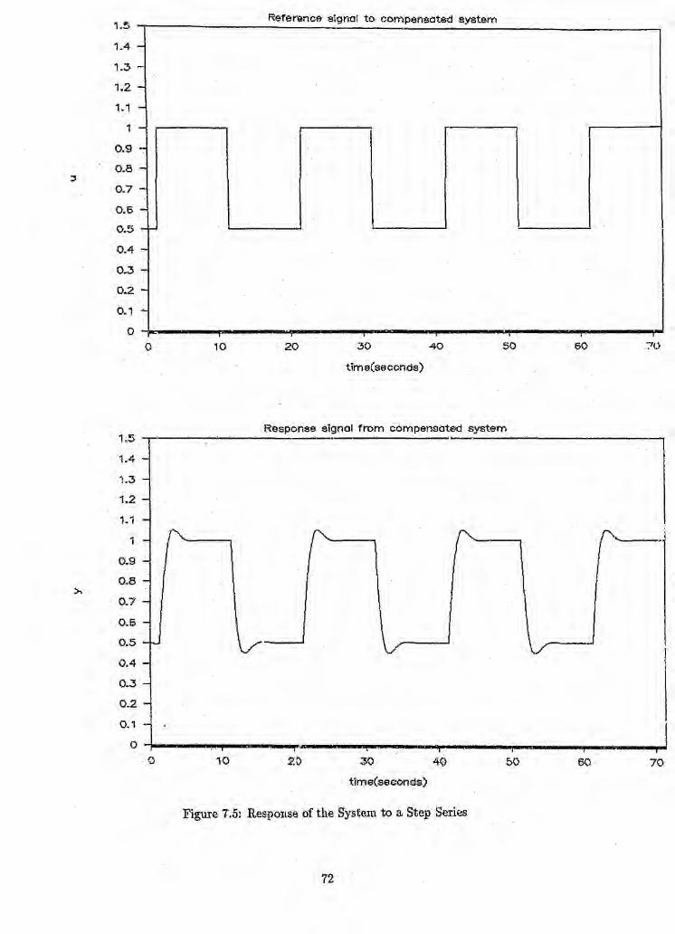
The open-loop system was excited by a rich input signal to ensure good conver-gence performance. The algorithm succeeded in producing a very good estimatedoutput y(.k) in comparison with the actual plant output Y(k} as it is shown in Fig-ure 7.1. The estimation error e(k) and dead zone a(k) are shown in Figure 7.2. Theerror is quite large at the initial stages of the estimation process. The fixed deadzoneark) takes the value ofl.O when the estimation error isgreater than the estimationerror limit eUm. The deadzone behavior follows the error e( k) very closely. Theparameter updating occurred mostly during the start-up period. This can, also, beseen in Figure 7.3. The parameters converge rapidly during the initial stages withonly sprradlc fluctuations during the later stages.
The algorithm produced the estimated parameters.
0.0 :::::1.009796
bo:::::1.012243
which represent a o"operator model:
8y(k) + 1.009796 y( k}::::: 1.012243 u( k)
The estimated model approximates the continuous time first order plant veryclosely. The estimated parameters are very near to the true system parameters.This is an indication that the 8-operatol: concept under fast sampling conditionsproduces good models of continuous time systems. It also indicates that the 8 == sapproximation is valid under fast sampling conditions.
65
It is understood that the very close tracking of the plant output by the estimatorand the very good convergence of the estimated parameters tothe real ones is influ-enced by the fact that the plant order is the same as the plant order the algorithmis designed to cater for, namely, to produce first-order estimation models.
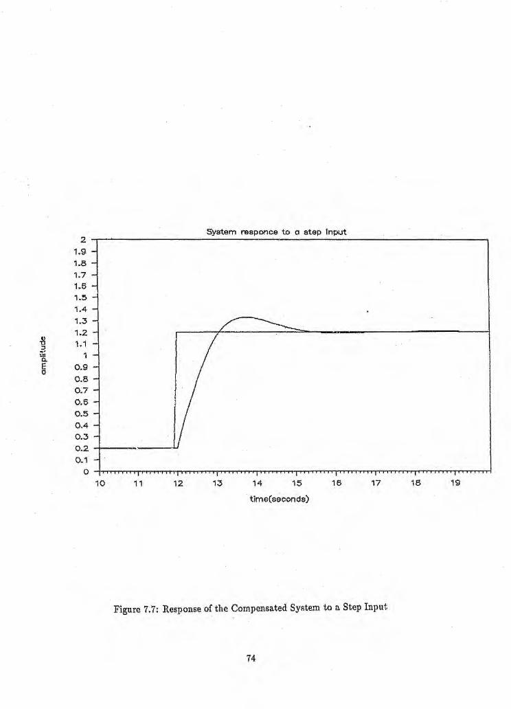
The open-loop system has a damping factor of ( = 1 and Wn = 1. The speci-fications for the closed loop system were a) percent overshoot PO = 10%, and b)settling time T« = 4 seconds. This resulted in
(= 0.5912
WIl = 1.6916
W3dB :: 2.9651
<Ppm = 59°The closed loop polynomial A" was given by;
A* = 0'2 + 2.00015 + 2.862
having the roots$1 = -1+ 1.36455j
8.2 ::·-1- 1.36455j
The roots of A"'(O') are depicted on a s-plane diagram SHownin Figure 7.4.The controller design parameters generated by the algorithm were:
J(p = 1.0000s, = 2.8615 or
Ti = 0.3495
The dosed loop response to a step input can be seen in Figure 7.7. The settlingtime of the system is less than four seconds and the overshoot is ten percent. It iscleat that the compensated system meets the design specifications. Also, Figure 7.5shows the response of the compensated system when the reference signal is a seriesof steps. The system is stable and the output follows the input signal smoothly.The algorithm generated PI parameter which produced very good tracking of thesetpolnt,
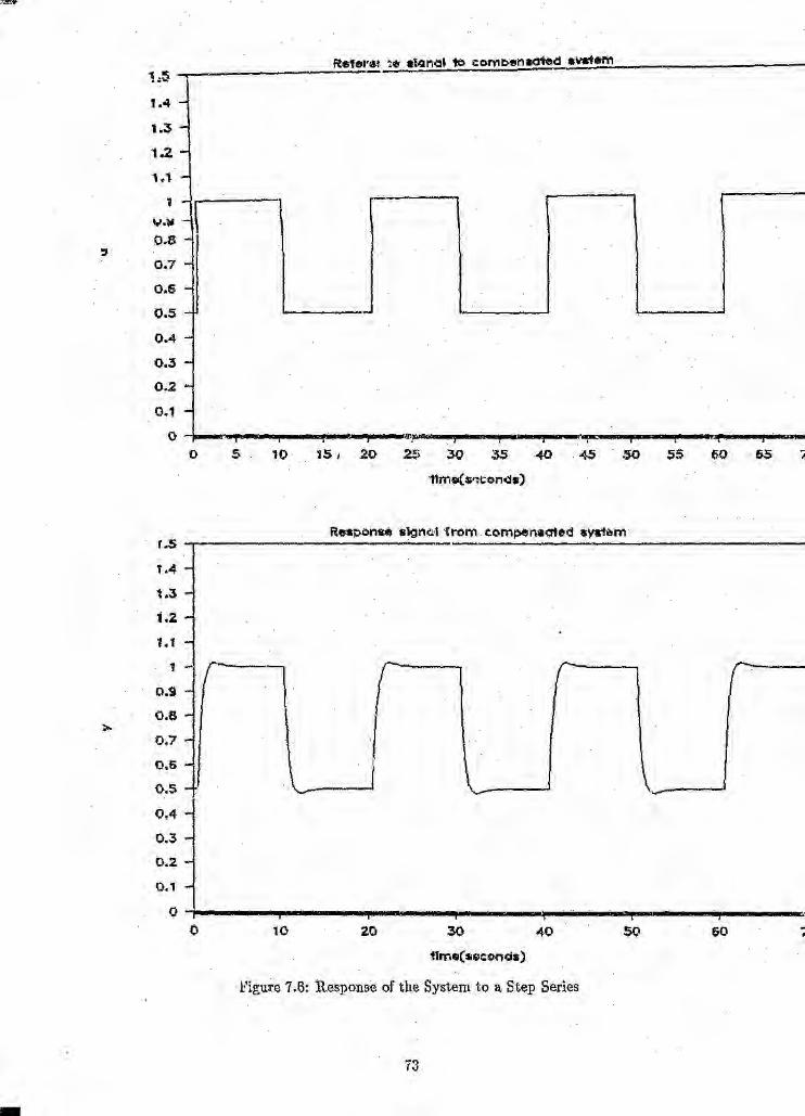
Next, the percent overshoot requirement was reduced drastically, but the settlingtime requirement was kept the same. The design specifications were PO = 0.3%and T" = 4 seconds. This allowed the system almost no overshoot and still requireda four second limit for reaching steady state. The controller parameters producedwere:
f(p = 2.000Ki = 1.4308 orTo = 0.6989,
Figure 7.6 illustrates the response of the compensated system to a series of steps.The system again tracked the setpoint in a satisfactory manner.
66

7.2.1 SummaryThe algorithm was used to model a first order continuous-time system. The es-thnator. produced parameters that were vp,ry dose to the 'true plant parameters,reinforcing the idea that under fast sampling conditions, th~ delta-model can ap-proximate the continuous-model well. The controller design produced PI parametersthat produce stable closed-loop system responses and good setpoint tracking.
67
1
0.9
0.8
0.7,
0.5A~~ 0.50.-£.-
0.4
0.3
0.2
0•.1
00
PIM of plelnt output V(k)
---. ..----
200 ..300
11m.
700
Plc:>t of estlmQted ou,p~ yhQt(k)
700.3aO
"mGFigure 7.1: Plot of Actual and Estimated plant Output Values
Plot of th~ ",lmct~d error eel()0.3 -r--,------~------------------------~------------------------------~
11m~
.2
1.91.81.71.51.51.41.31.21.1
0 1" 0.90.8G.70.50.50.4O.~G.20.1
0I)
2.1.91.81.71.61.51.4
1.21.1
0 1.n0.90.2-0.7G.50.50.40.36.20.1
0Q
'------'
too 700
11m.,
300
'In:ti'" """ .", """"" .
Fi{§Ull'e7.3: ;Pxat ef Es,timat~d Parameters aO and bO
500 700
70
,,\ ,..,,,.
\\\
"qJ r,( \ .
.~--------~~~~~------------------~,~--~;~.-.------------------------------------~----~,
j(.J$1 ;!__... .» __ ~_ t.3E'455
',. ,J ", ,. \. \, \) '-, \, ,, \, \,j,,'.',.f
,,.I,.,.
I,.r,.,.
,;Ie, ,
., II ,
',..,: r'";.: ;: "
, i'I I
I "'. ~,, v.'f.---------- ..-- --- .-'.-- 1.$6455
:',,' -; '4'»'"~i,g\iiTe7,4: !t<,x@tLf1cu:s oftlte Bystelu
1.5
104 -1.3 -1.2 -t, t -1 -
0.9 -0.5 -
;,0.7 -0.6 -0.5 -0.4 -0.3 ...
0.2 -0.1 ~
00
Reference sIgnal to cornpenected .systerT'1
1.5
1.4
1.3
1.2
1.1
1
·0.·9
O.B0.70.60.50.4
0~30.20.1
00
10 20 30 40 50 60
Response $lgnal from compensated system----~~--~----------~
time(secon ds)
J10
"os TFE"tf.
50 60 70
FigtU'e 7.5: Response of the SYstem to a Step Series
72
O.S0.70.6O.S0.40.30.20.1
o
e er~t ~eJ aane
----=\-I-----....
-JpJCW2ll ! ., , , -'''l- I I ' I I -
R f
1.4
1.3
1.2
1.1
1
o 5 10 151 20 30 .3S 4S 55 60 65
Re*J)on8f1 slgl'lOil 'from eompenscrted aya1em~---------~~-----------------, .S
1.4
1.3
1.2
1.1
1
0.9 -0.8
0.70.6O.S0.40.30.2.
0.10
0
r r
u10 30
tlm(l(.~t;ond:s)
Figure 7.6: Response of the System to a Step Series
20 40 60 i
73
-
System raaponce to a step Input2
1.91.8.1.71.61.51.41.31.2o
'U 1.1::l....1'£
E 0.90 0.8
0.70.60.50.40.30.20.10
10 11 12 1::; 14 16 1916 1715time(second$)
Figure 7.7: Response of the Compensated System to a Step Input
74
7.3 SimulationThe simulation used a second order system described by the differential equation.
d2 yet) + 0 5dy(t) + 0 2y·(t) = d~l(t) + 15u(t) + tP'r/(t) . d'r/(t) + 'net)dt2 • dt' dt' dt2 1"" dt "
Using the Laplace transform, the system becomes
(S2 + 0.5s + 0.2)Y(8) = (8 -I- l.5)U(s) + (S2 + 8 + 1) 1](s)
with 'r/es) the random disturbance signal.The algorithm was executed with the following fixed parameters.
We = 0.5 .LPF cutoff frequency
1::. = 1.0 Sampling time
);= 0.97 Exponential forgetting factor
peO) ::: 100.0 Initial value for the covariance matrix
0(0) = 0.0 Initial value for parameter vector
e = 0.0008 lIPF corner frequency
0: = 0.4 Maximum value for variable deadzone
fJ = 1.3 Variable deadzone scaling factor
0' = 0.98 Variable dead zone pole
eo ;= 0.0002 Threshold coefficient
el = 0.0001 Va-riable deadzone coefficient for input signal
e2 == 0.00005 Variable deadzone coefficient for output signal
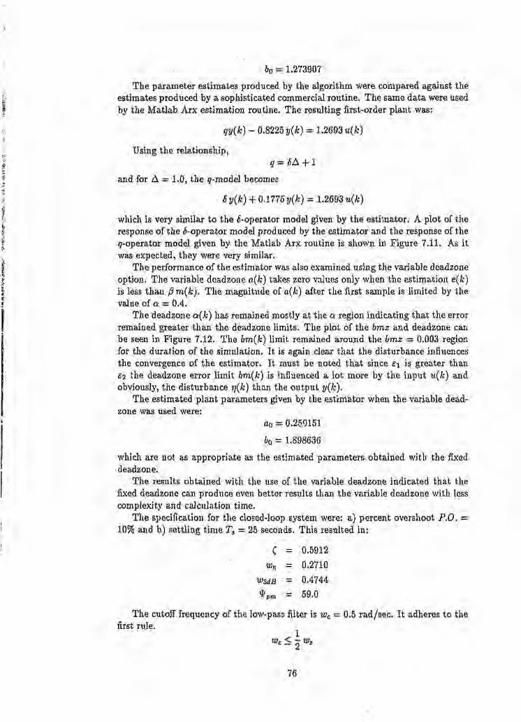
The algorithm was used to estimate the first order 8 model of the simulated plant.A series of very fast changing steps is used as the input signal to the process. Theplant output y(k) and the estimated output y(k) are shown in Figure 7.8 indicatinggood tracking ability by the algorithm. TIle low pass filter manages to partiallynegate the effect of the disturbance on the estimator. The estimation error shownin Figure 7.9 is substantially large .;'\1'\ expected due to the effect of the disturbance'r/(k) also shown in Figure 7.9.
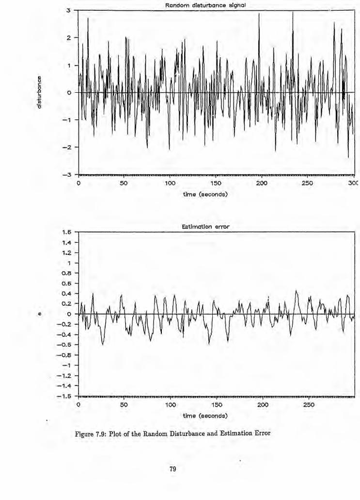
The convergence of the estimated parameters is also influenced by the randomdisturbance. Although they converge to the right region -iuite rapidly, the parameterupdating is sustained.Ior much of the simulation run time. The plot of the estimatedparameters is shown in Figure "(.10. The presence of 'I'J(k) Influences the convergingability of the algorithm.
The algorithm produced the estimated model.
8 y(k) + O.1723'l8y(k) == 1.273907 u(k)
withao = 0.172378
75
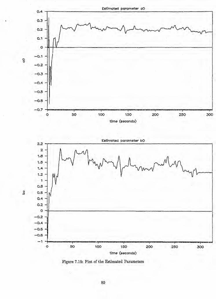
bo = 1.273907The parameter estimates produced by the algorithm were compared against the
estimates produced by a sophisticated commercial routine. The same data were usedby the Matlab Arx estimation routine. The resulting first-order plant was:
qy( k) .".0.8225 y( k) = 1.2693 u(k)
Using the relationship,s= ac.+ 1
and for Ll ;:::1.0, the q-model becomes
ay(k) + O.1775y(k) = 1.2693tt(k)
I11
iI
which Is very similar to the c-operator model given by the estimator. A plot of theresponse of the a-operator model produced by the estimator and the response of theq-operator model given by the Matlab Arx routine is shown in Figure 7.11. As itwas expected, they were very similar.
The performance of the estimator was also examined using the variable deadzoneoption. The variable deadzone Q,(k) takes zero values only when the estimation e(k)is less than f3 m(k). The magnitude of a(k) after the first sample is limited by thevalue ofc = 0.4.
TIle deadaone cx(k) has remained mostly at the cr region indicating that the errorremained greater than the deadzone limits. The plot of the bme and deadzone canbe seen in Figure 7.12. The bm(k) limit remained around the bmz = 0.003 regionfor the duration of the simulation. It is again clear that the disturbance Influencesthe convergence of the estimator. It must be noted that since E:l is greater thane2 the deadzone error limit bm(k) is influenced a lot more by the input u(k) andobviously, the disturbance 7J(k) than the output y(k).
The estimated plant parameters given by the estimator when the variable dead-zone was used were:
ao = 0.25,<)151
bo:::; 1.898636
which are not as appropriate as the estimated parameters obtained with the fixeddeadzone,
The results obtained with the use of the variable deadzone indicated that thefixed deadzone can produce even better results than the variable deadzone with lesscomplexity and calculation time.
The specification for the closed-loop system were: a) percent overshoot P.O. =10% and b) settling time T,= 25 seconds. This resulted in:
( :::; 0.5912w'l :::; 0.2710
W3dB :::; 0.4744q'pm = 59.0
The cutoff frequency of the low-pass filter is We :::;0.5 r~d/sec. It adheres to thefirst rule.
76

with W8. = 6.283 roo/sec and also to the second rule
In this case, We is almost equal to the closed-loop bandwidth so that the randomdisturbance does not influence the convergence of the estimated parameters. Thealgorithm ensures that the designed closed-loop bandwidth does not exceed the LPFcutoff frequency. .
The closed-loop polynomial A" was given by
A* :=; 62 + 0.32040 + 0.0734
having the roots81 = -0.1602 + 0.43704j
82 ::: -0.1602 - 0.43704j
The roots of A"(c) are illustrated in Figure 7.13.The controller parameters produced by the algorithm are given below as:
I(p = 0.1159J(i = 0.4963 orTi = 2.0150
The closed loop response to a step input is shown in Figure 7.14. The settlingtime of the compensated system is within the T., ::: 25 seconds requirement.
7.3.1 Summary
The algorithm operated under severe conditions caused by the presence of the ran-dom disturbance. It achieved to produce a good first-order model for the plantunder investigation. The use of a variable deadzone did not produce better resultsthan the fixed deadzone. Also, the robustness of the algorithm was enhanced bythe use of the low-pass filter. Finally, the controller design achieved to produce PIparameters that enabled the closed-loop system to meet the design specifications.
77

1.51041.31.21.11
0.90.80.70.60.50.40.30.20.10
-0.1~0.2-0.3-0.4-0.5
0
Plant output
' .. , ..... iI.... ' ........ wnw.ir·'·"·, .......... "··'·"r'·..•..•....'''·'D'i.' ... , .......50 150
time (seconds)
200
~stlmoted plant output
250
50 150
time (seconds)
100
Figure 7.S: Plot of the Real and Estimated Plant Values
78
•.. ·r'··iiM' ,•• ,1250
1
8c~ 0:l]"0
-1
1.6
1.4
1.2
1
0.8
0.6
0.4
0.2
0
-0.2
-0.4-0.6
-0.8
-1
-1.2
-1.4
-1.60
:5Random disturbance signal
2
- I-
I
- IAI
I,
Ji
- m~ ~I
--2
-350 30C100 200 250150
time (seconds)
Estimation error
.lilliiiii' •• ih.' VltlnnI., '.iii.iWii Wi•• ,f'••••••,.,,, "'W' •• iU•• ,ii•. a•• triiii •• ihU •••• 'riii •• f'1tI"ITII1IITII l'I'II1I'I!1mmo-m!
50 200100 150
time (seconds)
250
Figure 7.9: Plot of the Random Disturbance and Estimation Error
79
0.4
0.3
0.2
0~1
0
-0.10'0
-0.2
-0.3
....0.4
-o.s
-0.6
...0.70
2..2
2
1.8
1.6
1.41.2
1
0.8.8 0.6
0.4
0
.....0.2
-0.4
-0.6
.......0.8
-10
E$timated parameter 00
50 100
time (seconds)
100 200 200
Estlmated parameter bQ
t&iAi M".ttt,;J, •••• N••••••• iiDiIil·r"·.·.i\ii •• Ei ••• a•• r "' ,."1_'*'''" ••••• '' ••• 6 .. , .
100 150
time (seconds)200 250-
Figure 7.10: Plot of the Estimated Parameters
80
Estimated ~ystem (q=operotor)8 -.--------------------~----------~~---------~------------------~~
time (seconds)
rtstlmoted system (deltc-operotor)8 ~------------------------~--------~------------~----~------------~
o D~~~TM~MTTM~MT~i~ ..~,~.nil~.r'n"~'~"NrT.~TM~~TM~~~~~~~rlT~TM~rNTnMT~~MT~o 10 2.0 50 70 80 90
tlm$ (.'I3!~cbnds)
Figure. 7.11: Plot oi.th,e two E$~hW9ltedMadels
0.0025
NE O~OO2.0
0.0·015
0.001
0.00\0
1
0.9
0.5
0.7
0.5
2 0.5,_,.I;)
0.4
0.3
0.2
0.1
00
Variable bh"lZ
o ~.'••""'.'io 50 150
time (seconds)
200 250
vorh~ble dood2ione $:joino(k)
.n',....... Riiiiin .. .-•••• ".,IiE..····r'·U'Wbhi250
7.4 Real Plant Test
Th~ lPemer$aIH1e of th:e rugerJthm was examined using real-time plant data. Theaim of the test was to observe the behavior and robustness of the estimator underplant oper:a;ting conditi9ns. The Raw Gas Compressors Section of the Ammonia.Plant, located at the AIDe! Modderfontein Factory, was used for the estimator trialtests.
TIre two taw gas compressors deliver raw gas, produced by the GasificationSeGtion~tothe CO Conversion Section where the hydrogen needed for the productionof liquid amilloma is extracted from the raw gas, The compressors are driven bytwo,Dela.val s:tea!R turbines. The speed elf the compressors is controlled by twoCol'npiIies~orsControl Corporation (CCC) Load Sharing Centrollers. The 4-20 rnACOfi\bol \si!~al V<1l'!ier;the posi:tion of the stearn inlet mnltiports thus controlling theste~IIl, ~'f!>W ':i,rttothe. ,turbine., The lO,~a .s~tari)ngcontrollers are, part of a complexco.Ii!~lloL.,s~heme tha~ G.cmt:rolsthe load ,and;, cons~quently~ the speed ofeach compressorbased on thel~v.el of tIr~a;ccuimulated xawgas inside the Raw Gas Holder and, also,on t:11eposition of the oIt~l'3)tingpoint -of each compressor in. comparison tb the surgecu.t;:veo£,eac:li!,macill':ne.An f.Uustration ofthe process is given in Figure 7.15.
The eSjji;~Med modelJ'ehlltes the load sharing control signal to the steam. flowin't'G: vAe tu:r'lHne',Th.e pi'a'fit d;~ta used hy the esti$8ltot were taken' by sampling. the
c lQa® sIr~J'~fj;¢ont~QJ,sI~al (I1YB 8123) an:d .the 13 stream, steam flQw. signal (FIBSlOl)., .':Chesi~zy~s·w~r~~a;mpled ~very ten seconds, .•Thelopp was 0Jle7:atin~ underclosed loop ~qp:fti0n.S alnd. the cantrol signal was sufficiently act!· .... > was notnee~ssar~ ]0 J,njeci'a:ny l~indof sp.ecial.test. signal.
The estitnafn;~rwas set '1.!ipfbr the paratneter iden:tificatiol,\ test with the followingparanretells. d~zy~e~~. '
~)! ;;::'Q~ilt~fc~J~tF~te(,P:rency~~e~;;~:~~~.""+G~V~1"'.'"~*pplt~~'t~ll\LfongetJting1faGt0i'
~~@,~,== ~QQ·.~~t~~l!1y~¢ tor.(>JJ~arfl:lllItc¢fflMrj~
:~~(l)==1. \0~@f~*,~~,~qjllu~ !rQjc.:p,ata;:~¢jler·.V~GtpJ}.•, ",' :'!'., , ", - '·,c·· ',-' -~,- :j_ ," _,
~efJ~:n#,~E)quentc¥~ '" ...
.'.-~-;I."_;-' __.,_~
I

....cd
-:t,.... -----"Z" .:a
I \,.; 1 \~- f \.... .~<it.N
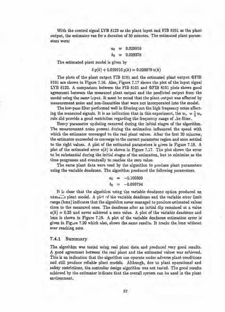
With the control signal LYE 8123 as the plant input and :nB 8101 as the plantoutput I the estimator ran for a duration of 50minutes. The estimated plant param-eters were:
ao = 0.029910bo :::; 0.028973
The estimated plant model is given by
8y(k) + 0,029910y(k):::: 0.028978u(k)
The plots of the plant output FIB 8101 and the estimated plant output @FIB8101 are shown in Figure ".16. Also, Figure 7.17 shows the plot of the input signalLYB 8123. A comparison between the FIB 8101 and @Fm 8101 plots shows goodagreement between the measured plant output and the predicted output from themodel using the same input. It must be noted that the plant output was affected bymeasurement noise and non-Iinearltles that were not incorporated into the model.
The low-pass filter performed well in filtering out the high frequency noise affect-ing the measured signals. It is an indication that in this experiment, the We = ~Ws
rule didprovide a good restriction regarding the frequency range of the filter.Heavy parameter updating occurred during the initial stages of the algorithm.
The measurement noise present during the estimation influenced the speed withwhich the estimator converged to the real plant values. After the first 20 minutes,the estimator succeeded to convergeto the correct parameter region and soon settled'to the right values. A plot of the estimated parameters is given in Figure 7.18. Aplot of the estimated error e( k) is shown in figure 7.17. The plot shows the errorto be SUbstantial during the Initial stages of the estimation, but to minimize as thetime progresses and eventually to reaches the zero value.
The same plant data were used by the algorithm to produce plant parametersusing the variable deadzone, The algorithm produced the followingparameters.
ao = -0.100309bo = -0.096794
It. I;; clear that the algorithm using the variable deadzone option produced anuns'Ltl,:":aplant model. A pIN 'If the variable deadzone and the variable error limitrange (bmz) indicates that the algorithm never managed to produce estimated valuesclose to the measured ones. The deadzone after an initial dip remained at a valuea(k) = 0.25 and never achieved a zero value. A plot of the variable deadzone andbmz is shown in Figure 7.19. A plot of the variable deadzone estimation error isgiven In Fig'.tre 7.20 which also, shows the same results. It tracks the bmz withoutever reaching zero.
7.4.1 Summary
The algorithm was tested using real plant data and produced very good results.4- good agreement between the real plant and the estimated values was a.c1).ieved.This is an Indicatlon that the algorithm can operate under adverse plant conditionsand still produce reliable plant models, Although, due to plant operational andsafety restrictions, the controller design algorlthm was not tested. The good resultsachieved by the estimator indicate that the overall system can be used in the plantenvironment.
87
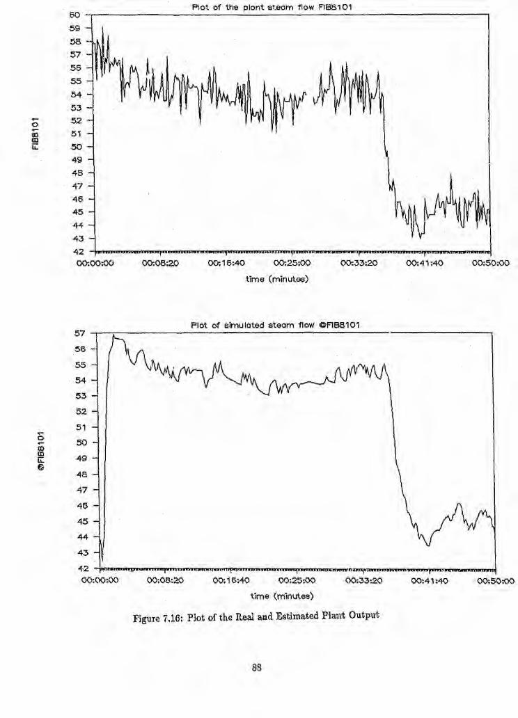
(; 52iO 5.1lDi:i: 50
494847464544
:~ -t-_ _...,.,.....,rrrn_,.,...., ""'mo,.""."_"""M"'""""••m.. m•• rto\i.,.. ·.·, ·,· ·_· • .. ·'.r" • ,..•..• " J00:00:00
575655
54
o~5251....
050....
IX)lD 49i:i:e 48
4746
4544434~
Plot of the plant stecrn flow FIB810160 -~--------~------------------------~~----~--"------~------------~59.
585751')
5S5453
00;41:40 00:50:0000;25:0000;16:40
time (minutes)
Plot of simulated steam flcw CFlB8101
00;08:2.0 0<);16;40 00:41;40
time (minutes)
Fjgure 7.16: Plot of the Real and Estimated Phtn:t OutlH\'t
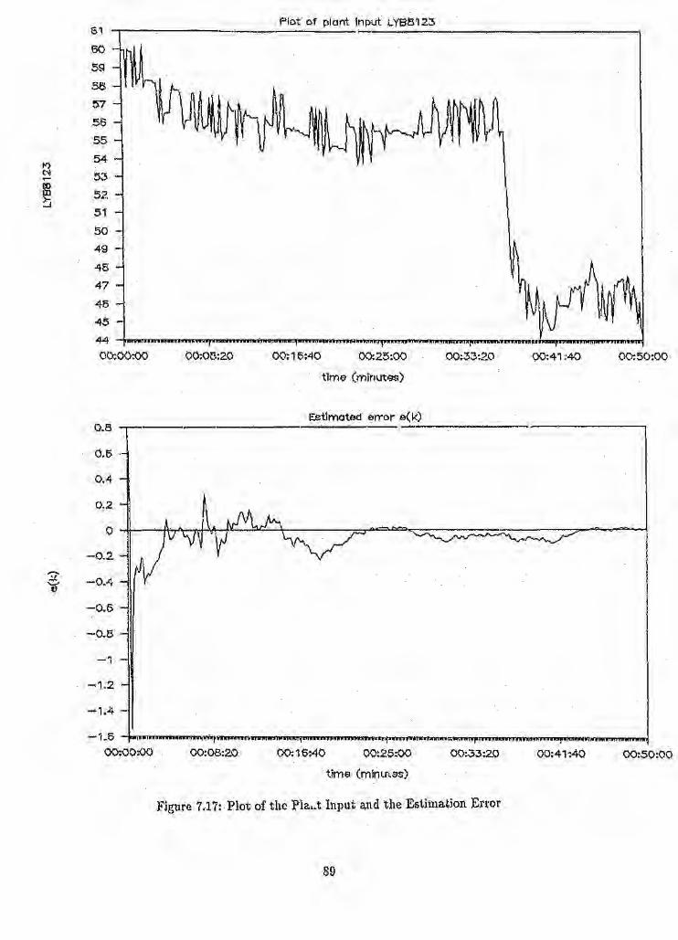
nN..-00In:J
-C -0.4t)
Plot of plant Input LY68123-r------------------~--~, ------------------------------------,61
60
5958
!57 -
56555453
5251
5049
48
474645
44 ~mm~~~~~~--~~~~---n~~~~~~00;00;00 00:06:20 00:16;40 00:25:00 00:33:2.0 00:41:40 00:50:00
time (minutes)
0.8 -r------ Estimated error e(k)
0.6 .
0.4
0.2
-0.2
-0.6
-0.8
-1
-1.2
-1.4 -
-1.6 ~~mm~~~~,~Mmmn~~""~~~~~~MnMm~~mm~~~~mm~~~~00:00:00 00:08:20 00;16:40 00:25;:00 00:33:20 00:41:40 00:50:00
time (minll'l.Ss)
Figure 7.17: Plot of the PIa-l.t Input and the Estimation Error
89
E:stlmoted pororneter 002.5 -r----------~~~------------~------------------------------------~
-3 ~~~~~mm~~~~~~~·~~~~~00:00::00
2
1
1.5
0.5
oo-0.5
--1
-;.5
-2
-2.5
00:08:20 00:16:40 00;25:00 , .' }:2.0 00:41:40 00:50:oc)
time (minutes)
o.0
2-
2.5
-2 .
.~-2.5 ;..rmm .....,,_.nn.w..,tii ..nqMrm',.. mdifl ,..,•• miiiMun "'!J,wrr., miill1fl.. m""''''''.ti''''.i4''''iia'.mliannu.,...,_...."IfnWT1IinIi'f'IinrTIIWnm'llIU.r' h.. ' •• 'wn t .. an i•• ,k ih1,diiil
00:00:00 00:08:2.0 00;.16;40 00:2.5;00 00:33:20 00:41:40 00:50:00
time (minutes)
Figure 7.18: Plot of the Estimated Plant Parameters
90
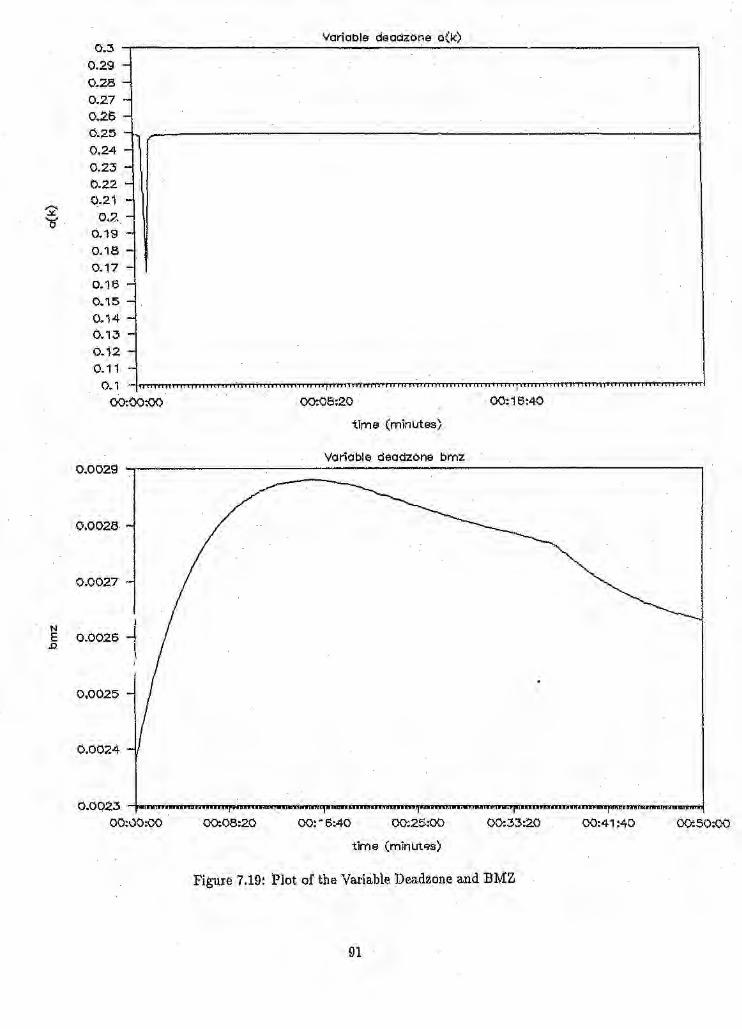
Variable deadzone 0(1<:)0.30.29 -0.2.8 -0.2.7 -0.26 -0.25 -0.24 -0.23 -0.22 -0.21 -
~ 0.2. -'110.19 -0.18 -0.17 -0.16 -0.15 -0.14 -0.13 -0.12 -0.11 -
O. 1 'I'
00:00:00 00:08:20 00:16:40
time (minutes)
Variable deudzona bmz0.0029
0.0028
0.0027
I
0.002610.0025
0.002.4
0.0023 ...,.... ....... UU ........ f .. p: ..... QiQ' •• , •• i•• '.Mi,.,.e ...... MriIiIl.hHiri..... 1U ..... ril•• i.fiiAC.'.ffl,i'.'.ri ..... "' ...... MriIi .......
00:\.)0:00 00;08:2.0 00:25:00 00:33:2.000:-6:40
time (minutes)
Figure 7.19: Plot of the Variable Deadzone and BMZ
91
00:41:40 00:50:00
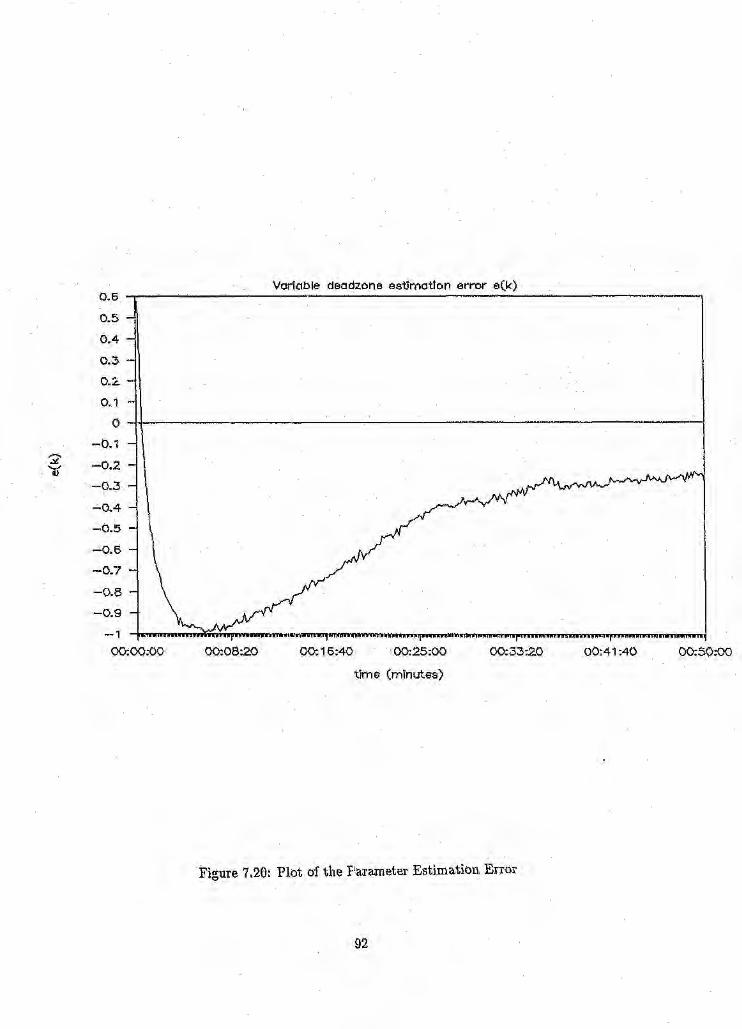
Vanable deadzone estimation error e(k)0.6
0.5
0.4
0.3
0.1
0
-0.12 -0.2.......01)
-0.3
-0.4
-0.5
-0.6
-0.7
-0.8
-0.9
-100:00:00 00:08:20 00:16:40 00:25:00 00:33:20 00;41:40 00:50:00
time (minutes)
Figure 7,20: Plot of the Parameter Estimation Error
92
Chapter 8
Conclusion
S.l General
The report has presented the philosophy and the design methodology of a robustautomatic tuning algorithm. This chapter gives a summary of the developments ofthe previous chapters and discusses some of the most important findings emergingfrom the research. Also, it lists a number of recommendations that can improve thedesign and enable its use in a real plant environment.
A review of a number of on-line parameter estimation and control techniqueshas been presented. The o-operator and its associated transform have also beendiscussed. The o-ope:rator was used to formulate the structure of the estimator andcontroller algorithms.
The robust estimator has been developed based on the general DARMA Modelmodified to accommodate random and unmeasurable disturbances. Techniques suchas the deadzone, the exponential data weighting, the Bierman U-D covariance fac-torization have also, been used to enhance the estimator's performance.
The controller was designed based on the closed-loop pole assignment principle.The USe of the o-operator facilitated the use of continuous-time design specifica-tions to he directly applied in establishing the appropriate closed-loop characteristicpolynomial.
It is believed that this research is significant in that a number of new conceptshave been successfully combined to produce a reliable algorithm. These are thefollowing.
1. Use of the o-opera.tor and its associated transform to formulate the estimatorand controller design.
2. It uses a generalized process model that includes measured and unmeasureddisturbances. The estimator is developed based on this model and its robust-ness improved by including in the normal algorithm the covariance resettingand deadzone options. Use of the U-D factorization technique to improve thenumerical performance of the algorithm. It, also, allows the user to vary thesampling time of the. algorithm.
3. Use of a low-pass filter and a high-pass filter to improve the signal conditioningof the measured signals and ensure the algorithm only receives information thatis vital to its functionality.
93

4. Use of a closed-loop pole placement method for the design of the controller.It translates the pole placement controller to an industrial PI controller andfurnishes I{p and K; parameters.
5. It uses continuous-time specifications to establish the location of the closed-loop poles.
94
8.2 Results of the StudyA set of simulations was used to substantiate the design work. The simulation ofa first-order plant produced excellent estimation and control design results. Goodresults were also achieved from the simulation of a second-order plant with theaddition of a random disturbance signal indicating the robustness of the design.The system produced good PI control parameters so that the specified dosed-looprequirements were met. Reinforced was, also, the concept that under fast samplingconditions the c-operator model tends to approach the continuous time model.
The estimator was tested under real plant conditions. The results emergingfrom the test were good. A good agreement was achieved between real plant outputand estimated model output indicating that the algorithm can operate under noisyplant conditions.·An observation arising from the behavior of the algorithm is thata good prior knowledge of the plant is desirable to avoid large initial estimationerrors. Also, the choke of the start-up parameters has a direct effecton the speedof convergence of the estimator and, also, on its robustness. The achieved resultsare of great significance in that the overall performance ofthe estimator reinforcedthe possibility of using the complete system in the plant environment in the future.
95

8.3 Suggestions for Future WorkAdditional work which may yield interesting results can be considered for the fol-lowing r, I~ J.
1. Improve the method of establishing the closed-loop poles using continuous-tiine design. criteria. A possibility is to use a knowledge based system whichwill provide the rules for the design of the control law.
2. EXPa.nd the system to design a second order pole placement control law whichcan he translated into an:industrial PID controller. Also, modify the algorithmto accommodate higher order processes.
3. Expanif the system to include a feedforward compensator design facility.
4. PerforJl). additional real plant tests and test not only the estimator, but alsoJhe controller design.
:AHl'illrge' hiflmber of r:hemicaJ.'facto;ries use computer systems for supervisory andcont.t<iilP'Ul']:r()Ses.• 1'lre a:vmlaMiTityof these computer systeme enhance the opportu-nities of using the algorithm in a variety of industrial applications.
One option is to use the algorithm in a self-tuning. mode, It could he usedto estimate the process model and to generate the required PI and PID controlp,arameters. The. calculated parameters could then be downloaded to the PtC whichare performing th~ actual plant control. Otherwise, the downloading of the controllerpar.almete].'sQan. be initiated by the process operator.
Another option is to use the algorithm in an adaptive controller mode where itmonitors the process continuously estimating the process model and adjusting theconttOllaw to cater for a new region of operatien.
Good results have been achieved by this work.however, additional theoretical andpractical research is required to guarantee a good and reliable system performancefor any circumstance which may arise in practice.
Appendix A
Bierman's U...D CovarianceFactorization
The Bierman 's U-I) factorization method is adapted to include the deadzone (b(k;)and the for,getti,nlgfantol' erCk)).
The otiginalltLS algorithm is:
iJ(k)
P(k -1)
ark ~ l}P(k - 2)¢(k - 1) . .... T= O(k - 1) + ..\(k -1) + 4>(k_ l)T P(k _ 2) ¢(k _l)'[y(k) - 4> (k - 1) 8(k - 1»)
1 .:[.... . a(k--1)P(k-2)cf;(k-l)</J(k ....l)Tp(k-,-2)= "\(k-1) P(k-2)- X(k-l)+4>(k-l)TP(k~2)4>(k~1)']
The RoLSalgorithm expressed in Bierman notation ;3:
X = X + k(~ - aTx)0' = r + aTPa, k = bPa/aP = !(p._ kaTp)
r
with r=forgetting factor and beerelative dead zone.By ract8ri:¢ing.P{k) as,
P(k) = U(k)D(k)UT(k)
where U(k) , and DCk) are the upper triangular and diagonal terms of the initial1118,'We' get;
ubfiTfJnuT
".'''' T-'.J_'f';= ![0nuT _ tJUvv U .1
r C!
= ~lulj) ....ba-1vvi]0 l. (A.I)
withf =v =:
a =
. fJTa = fI(k - 2)¢(k - 1)j;}f ~. . 1J{k _,.2)Jj(k - 2)tfJ(k - 1)
r + bvj;:;. r + b</JT(k- IJ P{k - 2)</J(k - 1),'," -i
withfJ - U (k ~ 1), (J;: '. U(k - 2)fJ == D(k _:l),D::: 1J(k - 2)
lllit!>t .!l,t1>m.et'hat D - bar 1VVT = fj f)i]T. For the assumption to he correct,'l!epla:$ing (:jj;fjjT in' Bq_,uai;ion 1 should~prod1tGe (JbuT. By Substitution, we get
_- . - .
1'4<11$We nave that:, = --a:. ,'~ -J: T '
}c "'; ,~./#t''!''''' "Jzy;,@llfl,,:, ~j lJ).,'f-' Qt¥ ' ",ViW', ,~:.4g.y.~e;"":~1'urner F(l:lttorization].;'0' -.. _,_ --" - - .~.:...
_.
l~t~ntt~lt¢,'~w~~~i!f,Ei'S4l:t:,we >s~e;,;t:h._2lt:'Ji»:e;~@,Jl;~tTuctionof tl,l.e up:c1ate u~nl~tQJls
~'~~~,~~" ~"&r.~'R
",\IJlg·t1t~Al~~_¢"iJfu:rJIer.fa(;tP;t1i:Ga:ti~il'a:dlj)l$t~dso as to coinoUh~ with out notMioll,
1= n,···2,....,1 (A.2)(A.a)(AA)
(A.S)
~qW~~·~~~,.p:,~wei~~t)Il'~'::';
(A.7)
(A.S:)
and
T.'. (Iv.l~ =--
at
t~l;:: .'1' + 'l:).j11
Appendix B
Alte'rnative Method ofE:x:pressil1g the PI Controller~....Operator Format
•In
The P1 controlier is giv¢n by:
u(t) == Kp[e(t) + ;iJ e(t)dt]
IfUl(t)~ iii e(i) then
U'tll(t) 1=s": Tie(t)
a,nd using Euler's ap:proximation, we get:
dl~l(t) ~ 'IL(/~+ 1) - u(k) == q ....1u(k)dt D.' . ~
where !J is the forward shift-operator.The analog PI controller can bA approximated by
where11.-
'~I - TiT}l'e transfer function of the discrc'te PI controller is
G( .) ....If I(.p1fiD. _ ...J(..;..p=(q_-_l...:..) __+,::-li......(p_I~...;..··iD._PI lJ - ~p + q .... 1 . - q':"" 2
Ustn:g lJ == 81:::. + 1 results in:
G' »i(.1:)._ 1(11.0 t lfp!_.(tPlu .... 6
whid\ Is the $.a.me :result acltieved hy dl;rectly substituting $ == c.
Appendix C
Formulation of the PolePlacement Controller as a PIDController
Assuming a second order plal~~.described by
B'lV(h) + aloy(k) + aoy{k) ;:: b10U(k) + bouCk)
and
• degree A::;: :2
• degree B:::: 1
• degree S ;::0., degree :0 ;:: 1
• d~!J'te,e.D;:: de!J'teeA - 1':;1
• degreeP;:: aegnteA. + de(JreeD + degreeS - 1 == 2
a.n.~d~gllee4;'" ::;: '.{..de"g't6ll.A+degl'(1eD + degreeS - 1 ;:: 4.'Xlhe ;pole pl?<tem.'eitt al'gari:tluu.pl'od1:lces the eensrol law,
@c(8).::;: ~g:9~:~:li!~Pn
The ,(l)naJ1c:>g :PIE) cc:>n:ttc:>lter ls ghten, by
ats)·.... .l(p(l + ~. +1{d~,S;)t J,'1" 'I'.r
J(·(l··. _:"_. ,..XIi:;[;.!-);;:. » ...+XtP+ N+Tc(s1 Ns
.::;:~i'p(~+'f.}8 + is +.~)
I( t s, 1#8).... r,p'\l + -; + $+1ir;
102
t,
where:
and ~ is the derivative filter.The transfer function can be written as:
0(.9) = I(p(s(s + ](d) + 1(i(S + I(d)+ NsZ)s(s + ](d)
= ](p(82 + 1(dS + ms + ](i](d +N 82)
= J(.p(N + 1)32,. ](P(Iid + 1(.)8 + Ii,J(dJ(ps(3+1(d) N .
By approximating, s = 6 we get
J(p(N + 1)82 + J(p(](d + J(i)3+l(j1{dJ(p .. P202 +P18 +PoS(s+J(d) . =- . 0(110+ Iv;
103

Appendix D
The Computer Program
The algQrithm was implemented using Microsoft Fortran. The complete program islisted below.
lCh
cCCC015DOl002003004005
006007
013008009010
THE HEADER Foa THE AUTOTUNING PROGRAM
WRITE(:i:,015)FORMAT(20X.'PRESS <RETURN) TO CONTINUE')READ (* , 001 )LAFO:Rl-iAT(20X, rz:WRITE(:I:.002)FORMAT(20X,'THE MODEL REFERENCE IS TYPE: COliiTROLLER')WR I'l' E ( :t tOO 3 )FORMAT (20X t· ' -:..- ....~------~-~----------~------- ... -----, )
WRITE.(':s:t 004 )FORMAT(20X,'THE SYSTEM READS THE PLANT rio AND THEN')WRITE(*,005) ,FORMA.T(20X, 'GENERATES A PLANT HODEL. THE MODEL' )W:RITE(:I:,006)FORMAT (2ox I •PARAMETERS ARE USED TO PltODUCt: THE')WRITE(:a:,007)FORNAT(20X,'PI & PID CONTROLLER PARAHETERS')WRITE(:t,0031WRITE( *, on 1FORMAT(20X,' .)WRITE(*,008)FORMAT(20X,'NOTE: YOU MUST SATISFY THE FOLLOWING RULES')WRITtH:I:,009)FORMAT(20X,' a. ItIS ~ 2wb ')WRITE(.;t,OlO)FORMAT(20X.' b. we s 1/2ws ')WRITE(:I:,Ol.3)WRITE(*~013)WRITE(*,015)READ(*,OO) )IAEND
105

CCCCCC DELTAC EPSHPC CFACTORC WCC ZC E1CC
EOGAM2
C GAMlC GAMOC ERRLIMC SIGMAC EPSOC EPSlC EPS2C NPARC NUVECC ALPHAC BETAC SiGMA1C DZL!MITC AZONEC ALPHAC BETAC PHIC THETAC KC ALPHAJC YHATC YHC UHC YC UC EC LAMDAC LAMDAOC YSPANC USPANC ENDCC
AUTOTUNER FOR PI CONTROLLERSUSING THE DELTA OPERATORCOMMENTS= SAMPLING INTERVAL= OUTPU'r STATE OF HPF FOR CONSTANT DISTURBANCE= INITILIZATION VALUJi:FOR THE U-O DIAGONAL TERM=: CUT-OFF FREQUENCY OF THE SECOND ORDER FILTER= DAMPING FACTOR FOR THE SECOND C:;',DERFILTER=: FiRST PARAMETER OF 'l'HESECOND ORDER FILTER= SECOND PARAMETER OF THE SECOND ORDER FILTER= FIRST DENOMINATOR PAR.AMETER OF THE SECOND ORDER FILTER·= SECOND DENOMINATOR PARAMETER OF THE SECOND ORDER FILTER= THIRD DENOMINATOR PARAMETER OF THE SECOND ORDER FILTER= FIXED DEAlJZONE PARAMETER= ADJUSTABLE DEAD ZONE PARAMETER= 1l:DJUSTABLE DEAD ZONE PARAMETER= ADJUSTABLE DEAD ZONE PARAMETER= ADJUSTABLE DEAD ZONE PARAMETER= NUMBER OF PARAMETERS= DIMENSION OF THE U VECTOR= ADJUSTABLE DEADZONE PARAMETER= ADJUSTABLE DEADZONE PARAMETER= ADJUSTABLE !lEADZONE PARAMETER= ERROR LIMIT FOR DEADZONE= THE DEADZONE= THE VARIABLE DEAD ZONE GAIN LIMIT= THE VARIABLE DEADZONE SCALING FACTOR= THE DATA REGRESSION VECTOR• THE PARAMETER VECTOR= THE GAiN VECTOR;:::BIERMAN U-D VARIABLE=·THE PRED1CTED OUTPUT VALUE== THE PLANT OUTPUT AFTER THE HPF= THE PLANT INPUT AFTER THE HPF= THE PLANT OUTPUT AFTER THE LPF= THE PLANT INPUT AFTER THE LPF= THE PREDICTED ERROR= THE EXPONENTIAL FORGETTING FACTOR= ADJUSTABLE FORGETTING FACTOR CONSTANT'"THE RANGE OF THE PLANT OUTPUT SIGNAL= THE RANGE OF THE PLANT INPUT SIGNAL= EOF
C+++++++++++++++++++++++++++++++++++++++++++++++++++++++++++++++C
C
C
C
CCC
INTEGER N,FINI,HPF,LPF,AZONEFLAG,LAMDAFLAG,NNHITEGER ))ZFLAG,INTERATIONREAL LAMDAO,ERRLIM,E,BMZ,MZO,MZREAL LPFF.(4) ,LPFBAR( 4) , atn ;MU2REAL Fl (4) t THETA (4) I K( 4) , DIAG (4) , OFFDIAG (6) , LAH.bAtALPHAJ ,.\ZONECOMMON/AREAl/FIt THE'rA,K, lHAG, OFFDIAG, LA~1PA,ALPHAJ,AZONEPARAMETER(SIGMA=0.98,EPSO=2.5E-3,EPS1=1.0E-3,EPS2=0.5E-3)PARAMETElt(ALPHA=O. 4, BETA:::l•3, CFACTOR=l 00.0, PI=3. 141592654 )
WRIT.!!:',*,001 )001 FORMAT(ilX,'':eHE OPERATOR IS TO DEFINE THE FOLLOWl:NG VARIABLES',).
106
WRITE(*IOO2.)002 FORMAT(21X,;~=========~======================================')
PRINT;t,' •PRINTlI:,'•PRINT;:,' ,WRITE(*.003)FORMAT(2lX,'PLEASE DEFtNE NUMBER OF PARAMETERS;a)2.b)4')READ(:t,004)~FORMAT(I2)WRITE(*,005)FORMAT(21X,'SET HPF FLAG:FLAG=l(HPF IS O~).FLAG=O(HPF IS OFF)')READ(;t,006)HPFFORMAT(Il)WRITE(:t,007)FORMAT(21X. 'SET L1?F FLAG:FLAG=l (LPF IS ON),FLAG:::O(LPF IS OFF)')READ(t,OOS)LPpoFORMAT(Il)WIUTE(*,009)FORMAT(21X,'SET LAMDAFLAG:FLAG=l(CON. FORFACJFLAG=O(VAR.FORFAC), )READ (* ,010 )LAMDAFLAG 'FORMAT(ll)WRITE(;I:,Oll)PORMAT{21X.'SET AZONEFLAG:FLAG=l(CON.DZONE),FLAG=O(VAR.DZONE)~)READ(*~012)A20NEFLAGFORMAT(Il )WRITE(t,070)FORMAT(21X,'SET THE OUTPUT ZERO-BASE AND SPAN')READ(t,071)YZERO,YSPANFORMAT(F6.3,F6.3)WRITE (:6:.072)FORMAT(21X,'SET THE INPUT ZERO-BASE AND SPAN')READ(*,073)UZERO,USPANFORl~AT(F6. 3, F6 •3 )WRITE(*,074)FORMAT(2~r 'SET THE SAMPLING RATE')RE:AD(t,O}:J)DELTAFORMAT(F6.3lWRITE(;I:,076)FOR~AT(21X,'SET THE We CUTOFF OF THE LPF')READ(*,077)WCFORMAT(F7.4)WRITE(*,078)FO)\MAT(21X,'SET THE WIlliRESTRICTION FREQUENCY')READ(*,077)WL
003004
005
006
007008009
010
011012
070011
on073
074
075688076077078
CPRINT;t:,WC,WL
cc ....- __- ....._~_, .... ... .... -'-_CICt PAR.T ONE:CI INITIALIZERCtCICI rC I -----~-------- ....--_-_----_. - .~_~ ... ICC
,CNN=(N:t;'o,') )/2TIME=O.OINTERA'l'ION=Ol\LPHA..)"::::]'•0IF(N.EQ.2)THEN
AO=O.OBO=O.O.YHll'l'=O.O
107
ELSEIF(N.EQ.4)THENAO=O.OAl=O.OBO=O.OBl=O.OYHAT=O.O
ELSEPAUSE'NUMBER OF PARAMETERS MUST BE 2 OR 4'STOP
ENDIFcC INITIALIZATION OF THE RLS VARIABLESC
IF(HPF.EQ.l)THENEPSH=O.0008XHPY=O.XHPU=O. "
ENDIFcC INITIALIZATION OF THE LPF .VARIABLEC
80
WS=2.0~PI*(1.O/DELTA)PRINT:I:.WS
IF(WC.GT.O.5*WS)1HENWRITE(:t,080)FOR1'1AT(21X,'THE WC IS GRE!TER THAN 1I2 WS RE-DEFINE WC')GO TO 588
ENDlFIF(WC.GT.WL)THEN
WRITE(*,31)FORMAT(21X,'THE we IS GREATER THAN WL RE-DEFINE WC')GO TO 6fjB
ENDIFALPF=WG/SQRT(2.0lMUl=(WC**2)*(DBLTA**2)MU2=ALPF:t4.0*DELTAE2=4.0+MU2+l-IUlEl=«2.0*MUll-8.0)/E2EO=(4.0-MU2+MUl)/E2GAM2=MUI/E2GAMl=(2.0:tMUl)/E2GAMO=MUI/E2
81
c
DO 16 I=1..4LPFF(I)=O.OLPF13AR(I)=O.O
15 CONTINUEC
IF(LAMD!FLAG.EQ.l)THENLAMDA=O.970
ELSEIF(LAMDAFLAG.EQ.O)THENLAMDA=O.9S0
108

Ll'.MDAO=O.985ELSE
PAUSE'LAMDA PLAG MUST BE EITHER 1 OR O'STOP
ENDIFc
IF(AZONEFLAG.EQ.l)THENERRI,.IM",O.003AZONE=l.O
ELSEIF(AZONEFLAG.EO.O)THE;NSIGMA1=1.0-SIGMAMZO=EPSOAZONE::l.O
ELSEPAUSE'AZONE FLAG MUST BE EITHER 1 OR 0'STOP
ENDIFc
OPEN(UNIT=l,FILE='PLANTY')OPEN(UNIT=2,FILE='PLANTU')OPEN(UNIT=3,FILE='PAR.DAT'.STATUS='NEW')OPEN(UNIT=4,FILE='IO.DAT',STATUS::'NEW· )OPEN(UNIT=7,FILE='PHI.DAT',STATUS='NE;W')OPEN(UNIT=8,FILE;::'THETA.DAT',STATUS='NEW· )
cc
, C_~ .... ........ .... .~. _
CCC PART TWO:C ESTIMATOR AND CONROLLER DESIGNCCC •C ..... • _
CCC500 INTERATION=INTERATION+l
TIME,=DELTA*INTERATIONc
CAL,L GETOHT (YOUT t FINI )YXX=(YOUT-YZERO)/YSPANCALL GE;TIlHUIN )UXX=,()JIN-UZE:RO)IUSPANIF(HPF.EQ.l)THEN
YB=YXX-EPSF1*XHPYXHPY=XHPY+DELTA*YHUH=UXX-EPSH*liPUXHPU=XHPU+DELTA*UH
ELSEIF(HPF.EQ.O)THENYH=YIXUH=UXX
ELSEPl1.USE'HPF FLAG MUST BE EITHER 1 OR 0'STOP
ENDIFc
IF(Ll?F.J'.:Q.l)THE~QY;:;GAM2:+:YH+GAMl:+:LP'FBAR(1)+GAMO:t::r./PFBAR(2)Y::::...EhLPFF(l )-EO:+:LPFFC2)+0'1LPF:F,(2 )=LPFF (1)LPFF (l. )=yL1?P'lM.lt ( 2 ) =L1'lP'EAlt ( 1 )
..LPFBAR (1 )=Y8
109

QU=G~M2:tUH+GAMliLPFBAR(3)+GAMO;i:LPFBAR(4)U=-EltLPFF(3)-EO:tLPFF(4)+OULPFF (4 )=LPFF (3)LPFF(3).=ULPFBAR(4)=LPFBAR(3)LPFBAR(3)=UHELSEIF(LPF.EQ.O)THENY=YHU=UH
ELSEPAUSE'ijPF F.i:.AGMUST BE EITHER 1 OR 0'STOP
ENDIFc.c
c
IF (LAMDAFLAG. EO. 0)THEN .LAMDA=LAMDbLAMDAO+(l.O-LAMDAO)
ENDIFIF(UONEFLAG.EQ.O)THEN
MZ=MZOBMZ=aETAtMZMZO=SIGHA:tMZ+SIGMAh (Hi..O+EPSl:tABS (UH) +EPS2tABS (YXX) I
ENDIF .cC THE GEN!RATION OF THE PREDICTED ERRORC
YHAT=O.ODO 20 hl.N
YHAT=YHAT+(THETA(I)*FI(I»20 CONTINUE
C
cE='{-YHATIF(AZONEFLAG.EQ.l)THEN
IF(ABS(E).GT.ERRLIM)THENDZFtM=lAZONE==l.O
ELSEDZFLAG=OAZONE=O.O
ENDIFENDIFIl"(AZONEFLAG.EO.O)THEN
IF(ABS(E).GT.BMZ)THENDZFLAG=lAZONE=(ALPHA/E hDEAD( -BMZ ,13MZ,:g}
ELSEDZFLAG::O
ENDIFENDIF
c
cCALL LS(Y,U,N,DELTA,DZFLAG,E,AO,Al.BO,Bll
CWRITE(*,lOOlAl,AO,Bl.BO
100 FORMA'rOX,FlO. 6,lX,Fl 0.6 t 1X.Fl 0.6. lX,FIe. ~1WRITE(3;200IAl,AO,Bl,BO,YH,UH
200 FORMATH'lO. 6 ,lX,FIO. 6 ,lX,FlO. 6 .rx.n e. 6 t ix, FlO. 6, lX,F10. 6)WRITE(4,ZOO)Y,'fHAT,lt.K(lJ,K(21,K(3)WRITE(?, 200)Fl (1) ,Fl(2) ,FI (3) ,n(4) ,AZONE,BM~WRITE( B,2J 0 )THETA( 1) t THETA ( 2) I THETA ( 3) I THET.A.( 4)
210 FORMAT(lX,F13.10,lX,F13.10,lX,F13. 10, ix.n s.:0)c
I).1'(FIN1.SQ.0.AND. TIME.LT.24000.0)THEN
110

\:IV !V .)uvENDIFCLOSE(3.STATUS='KEEP')CLOSE(4,STATUS='KEEP')CLOS~(7,STATUS='KEEPtlCLOSEr~8.STATUS = , KEEP' )
~. GENERATION OF THE CONTROLLER PAlWfETERSCALL COltTROL(AO,Al,BO,BliN,WCl
S~OPEND
~.FUNCTION DEAD .FOR VARIABLE DEADZORE VALUES
FUNCTION PEAa (BM:~L IBMZH t ElUWR 1REAL BMZt,BM,ZHtERRORIF (ERROR. LE. BMZI,l'l'HENDSAD:::ERROR-13MZ,L
ELSEIF(:ERROR.GT.BMZH)'1'HENDEAD:::ERROR-BMZH
ELSEDEAD=O.O
ENDIFRSTURNEND
SUBROUTINE GETOUT(YOUT,F!N)REAL YOUTINTEGER FlNREAD(1;400)YOUT
aeo FORMM'(F15.l0)lTi't.NOT. EOF(l))~HEN
FIN,::ORUSE
F!'H:;:1ENDUREJI'URNElll'
400
SUBMum:UlE G'E;TIN (UIN)itE~f=_UIN19~1:lC2t 4.00 lUINF0lUiAT(FlS.10)RE:reUiRNgND
,.,.S:J:L VTINE LS(YtUtNtDEt'llA,IllZFLAG,PER1ttAO~AltBOtBl). .. .. P~F:~~'I·;~ . . .. .
PJEl.L. lJ:~Rlt,tY.tP:,A.l.M .si ,B:O; DELTi\.R:E1tiI;!;.~JJ4J,'J.ltt 4Jt~( 4) ,Dl.AG( 4) I OE'FDUG( 6) ,LAM!)A.ALPHAJ ,M.ONEC·O~ONl~~'E~ll ' • I-{<EjlA,K, DIAG, OF~rirAG, LAMl},1\,ALPH!J, AZONE
111
,"
".;.'.
3D
11' I vt.,!, LAl>. r:U. 1 J 'l'H~.hFJ=FIO)VJ=DIAG(l):tFJK( ll=VJALPHAJ=l.O+VJ:tFJDlAG(l );::DIAG( 1 )/ALPHAJ/LAMDAIF(N.G'i'.l)THEN
KF=O1\U=ODO 20 J=.2.N
FJ=FI(J)DO 30 1=1• .1-1. KF=KFtl
F,i=FJ+FI (I·lt·OFFDlAG(KF)CONTINUE~J=FJ*DIAG (J IK(J)='JJAJLAST=ALPRAJALPHAJ=ULASTt V;Jt.F JDlAG (,j l=D1AG( J ):t.AJLASTIALPHAJ / LAMDAPJ=- (:.FJ*A:ZONE) IULlST0.0 4,0 1=11.1-1
lW::;KIJ+lW=OF'l;?Jl!AG(l{U)+I{( Il:tPJ:K:(iEl=K(I)+O}lFOlAG(KU):tVJOFFDIAG(KU)=W
CQ,NTINUECONTINUE
EN'O!F·ALPHAJ=ALPHAJI· :'()Jg)';l
EN'PIFI;F'(>i:!'ZFr.AG. EQ.
l\LPUAJ·=l • 0PO 50 l=l tN
Kfll=O.OCON'l'INU;E
EN:lliF
4020
50
60
00· '60 .,l:;:l , N. ['ali:'l'~(1 )=Tij~TA( I) +~E-1U<:tK( 1)/ALPHAJ
QQN'nU].1,l;E;·$:~{N•.E9.2 )'l1ijEN,;~(!!~"''l'R~T:Af1)8!01=TH1';'1'1.( 2 )
i~,ij"O)lF. ;l,F:(i.li. ElO,;4')"ll!i'~N
~." ,:''l1,l,~='''!J!H'E''l,'A(1 )'~O'7,_THt;'\I'A ( 2 )
.'·.'fli19!flii~!l1A(3.).,i.:~'QJ='J11l~'~A(,,4;:)
·:~~N.~lc~
'~fJ)~lF't~,,~,~!.~,J'Ta~N'''',';:,lp:,lE (:~ ~:?~l t,l )'i:,a:~m~*,Y
799
. 8,00
END
SUBROUTINE GONTROL(Ad,Ai,BO,Bl,N,WC)REAL MPW, l(p ,KIP.AR.AMETERtJ> I =3 .141 5926 54 )
100001
WRXTE(* I 001 )FORMAT I2l XI ' _~ ........ .., ... ........._......._...__.. J. }
PUNT :1:,' I
PR.INT *,' ,WlU'l'E:( tt 0(2)FORMAT(2U.'THE lISTI!!ATED PLANT PARAMETERS ARE:')PRINT :t.' ~Ili'CN.Ea. 2)T}{EN
WRlTE( 11:,003 lAO:FORMk'}:'(42X, 'aO=·,F10.6)W:RI'P,iH*,O(4).BOF:ORM~T'(42YJ 'hO=' ,FlO. 6)
ENPIFIF (N. EI)):,.4 )TIHn~
WUT:E(,:t,OOS)AOFORMATt42X,' a,Q:::' ,FlO. 6)WRITE(t,O'OS)AlW~ITE (:t tOO'S) S:OWlUT·E{*, 005 )21
EijiDIFWRr'l'E(t,799)FO:RMA'l'(2lX, 'OK=1 ELsll: 0')REAI),'(i t MD ) 1<1<FORMA'1.'(I1 )IF(KK.EO. 0 )THEN
:RE,M~(*,aOl lAO,!l ,BO,lllFORMAT (l~l0.6 t FlO. 6. FtO. 6, FlO. 6)PRIN'l':t,AO,BO~NiD,IFPRINT :tt' ,PRINT't, I I
Wll.I'l'E.( t ,0!l7 )FO~MiA'1.'tZlX, 'PRESS ANY KEY TO CONTINUE')ll.ll:'A:Ptt,600)LA'~F:<:),RMlll'12lXI l2 )PRUI',h,' •l?1tI\N:T!~l' J
WR;l\rE(j..'OO)F0~T ( ~JX. •THE CO~\rltOt, l?ARAME1'ERS MUST Bl': IN ltEArJ FU:JMBEP.S·).tl~N'!.niCrl' ,PIt!N,1~~I' .;WU'l'E;fi• I0:0:8 )F'ORH,p..T ( 21,l(, 'PEFIN:E' :IJJ;H~ DEJiSl·ltlgD }?5Ridlt'NT OV~'RS'ROOor')ltEAl)I (~*I Q1('),9ll?,O .Fo.~HtA::r:lr;'6• 3 )
JO).. '. .... 'Xt"ln';'F1iN'E ~ltE aE'SI.lt~fl 'S;~'l''l''lJIN~ 'rIME'),Il:~~P(:t!,lelll )"1':S :'.f\O:~'M~\'l\I(iU:&')3 )J;1lt~;R:V-);,. 'I ,
ltll:iliNIlMi,' ,
002
00.3
004
007
6,0'0
O:OS
009
01.0
OLl
.," a~((LOG('POll 00. (')).,* ("'1. 0) ) Il?H:tl\i2
\ l'I '~;~'~'""~~!.\'" ';(1"" " :n~l\ j -J ..... ~'f"
113

oeo CAL13ULATION OF TI{E PliASE MARGINC
e
~....
012
0'13
Ol4
IQ,1OJ
O,lS
("ZiPl )/SQR'I' (1. 0-Zu2) );)'t:S'THE PERCENT OVERSHOOT ACCEPTABLE?')
.mrt:rmi\'/(+ > j!,,:n1 fPC)!,p,EltClmT OVEMiIOOT=' ,1"6.3)
ELSE l?ltgSS ....0....·)
e\0', ,G);'l1G.tJ\l"J!:Tl;~N: (liE TilE N,A';rUJl{A.L FREOI1:e:N:CY,~" .
ti,0 Cl'Ai':tG.l:1:)JA'rI·!O,N OF Tlil! PE:M< AM1>t.I'I'UTE;~. '~;~W'=l..,al (2 •ad i (,S¢Rtt'(l •0- Z·lt-* 2) ) )J@ .. '" . ' ....re '~A,~(lll,:L~'W'I:()NOF 'l!ltll: RESONANT Fl,tEOll,ENCY.'.~ W!E,:::wrti~;$'qlV1Hl. Q.. (2. OtZ:tll:2)),~ . .
'0 ·~~~~l1,rtA\'l'L.QJl"P'~W:fl£ QUIll~n'FRT$QUEN'C'l (3d)))'~,.' . ,
wai~~'~.w.~,*~,SORT((bt2) +1.0) +Z)
I
We: <1>1J $ij!E S¥$T'EM IS GREATER THAN FU/l'l):~itlU~!~:'R$''F'~E0.l:1$NQ!l{ltE-·PltFl1Ui! Tltn SETTLING IflME')
.'{~a:~~,lX.· ~:;;i i Fa. 4 ,IX. j l?M=I ,re. 4 )
."-~a,,.'4'•.t'X I' WjR~'t 11'8.4.1 Xl )·w3DJ3'~' .ra, 4,)
114

lF~N.EO.2)THENAlST~.,::a. OtZtWNAOST:AR=W.Ni t 2
cPi ::::(AlS1IM~ ....AOj/BOt>O:::A.O'STldtlBO,e
'i' K:p=Pl! ~.1;1:::1>.. 0.)/~P
'.·tte! WRl'.l':lH*.(20)Kl,),K!
;,FO:R.MA;T(lX, -6AJN Kp=',FB. 4,1 OX, ' INTEGRAL GAtN Ki=t ,ta. 4.)"ENr~~I~F. .
lliE'lIlliRllt·Uip
;;,."'
I
References
[1] J" (j, .Ziegler a.nd N.•B. Nichols. Optimum settings for automatic controllers.J&$!/;fE 'lr.a/fI,S(1,G.tf;b.ns,64:759"-76'8; November 1942.
,~~JtiI·. ::qj. ¥ii,~gl~l;.<\.nd N.. B. Ni~ho16., Process lags in automatic control circuits.iJ/6-fMI/IJ '!J'tq.nsaeUOJ1sj 4.33-444, July 1943.
, " .. .:"~, .;'.'. ' , .
t3~ E,!'i',~". .$ihhl-skey. process Contn# $yst~ms. McGraw-Hill, New York, seconded~t!'on, 19'79.
(41 O. H. Cohen and G. A. Coon. T.lieoreticaJ considerations in retarded control... Pt,iyioitinslrUtnants Oo. Bull. No. TD$-10AI02.
[$[ P.liazebro~k and B. L. Van Dsr Waerden. Theoretical considerations on thet:>.pthnutn ad5ustment of regulators. ASME Transactions, 309-315, Apri11!'>50.""j,y :':'\}:'" '
~(j;]•n., E. Kalman. Design of a sell-optimizing system. ASME Transactions, 468-4iNS1FehjiUa;ry1958.
[1] t<. J, Astrom. Theory and applications of adaptive control. Auiomaiica, 471-Lit"; if8'~{$~ptelnihet1~'33.
f8J ~. Pete:rkg,. Pl'edktor-based aelHuning control. Automatioa, 39-50, January.' ilf9S4.
m9~~;. 'WI piatlte alta P. W. Gawthrop. Self~tuning control. Proc. lEE, 633-640,"'i y.... ;;r'Uitt~jtr9}7i9.·i•.:
.,', " ,",':":.'": ""'''':-,'
[X~J~"·~'P~r$()fi'.'!·$elr-tunillgl'egul~tol'Sfot a class Qf multivari(1,hle systems. Auto~. ", ~j:#:I(t(ilj";~'09""2l$.,;;\Nt~tGlLJ,9fl'!'J~.
:filtj r. ca, ., '. P(!;N1Jt:J).etet es'tjm1a;tion for GOlltj'nuous-tilne Jnodels-a survey. Au~':Hi ~!,i:'m~~tt;~1h>l:V4~~~i;ili9,8a'f;,< ',""'\ A
,['tl.~]~t';6·. '•..~J~a;~iri~d It.; f '~1~;.'"AidapUve"}t-ilterlng .Predict'ion and Control ..' ll~ePiiiip~~<U[ [.ne.\ ·J.®8'!E!· <,
" '. ,:;.,.~:t:I~,':',i\;:~:", .' ", .,'. _. ... . .r+3~ ~;. (;"1,:~90g:Wj.t} .,Ql1ld 1;(. S. 8'i1\.
~l'en\~i,t!.e~l-~al[I{tc" 19$'4.
Wl4] t. ;F., 11,~aga.:riID. ~,. Sehol;~a;n,ds, L. Sl~a.h.Adaptive controlstrategies for processQ(;)n$~c;;i~a Slll'V~~. AJ?GltEi a~l~C\. 6;!,~gl-91.a, 1996,.
.Adaptive FUtering Prediction and Control.
...fl:Sl !l,.:\(1l~i,lJaa.):t, -, .~ver aa;atP,tjv~'(lQ)i'i'I'Ql' 1ll.gpri'tll'll1N1.tutori al. Automatica,$8~lij;;_$~8'1&e ehtb~1":tg'$~.
[16J L. Ljung T. Soderstrom and I. Gustaveson. A comparative study of recursiveidentification methods. Dept. OJ Automatic Control) Lund Institute of Tech-nolog1bReport 7427:, 1976.
[17] 1. M. Ma.cLeod. State space modeling and control. Course Notes, 1987.
[IS] G. C. Geodwin D. Q. Maynes and R.. H. Middleton. Rapprochement be-tween continuous and discrete model reference adaptive control. Automaiica,22 No2:199-207, 1986.
[19] R. l'(. MMdleton and G. C. Goodwin. Improved finite word length characteris-tics in digit;ti control using delta operators. IEEE Transactions on AutomaticControl, AC..31 NollI101.5-1021, 1986.
[20]1. M. MacLelld. Delta operator. Oourse Notes, 1990.
[:~lJ1\.. J. Asttorn and :a. Witsenmaek, S¢lf-tuning controllers based on pole-zeroip)lruGemeltt.P·fOC. lEE, 127:120-130, 1980.
[221 I. M. Maritaod. Msc thesis lectures. Notes, 1990.
t [23] G. J. Bierman .. F'actorization Methods for Discrete Sequential Lstimation. Aca-demic Pre~si 1977.
f~41G. C. Goodwin and I{. S. Sin. AdaptiVe Filteri~ig Prediction and Oontrol.Prentice-RallIne" 1984.
['~&l G. 'E):a,nk1in and J. Powell. Digital Control 0/ Dynamic Systems. Addison ~W~sley, 1981.
[26] G. c.. (dl!)pdwin and K. S. Sin. Adaptive Filtering Prediction and Control.Prentice~l;t:a1i1Inc., 1984.
~~7JM. L. B'(.~r~,$'itsen.The implementation of. a generalized robust adaptive con-. .trttll.er. MiSe Th&$J$,lflits Unt.ver$itYl Witwa.tersrand; South Africa; 1988.
;&~~fl{.~••~§"tW~tn~l.}il;PllissQnL, '"jun,g <Lndn.Wittenma,rk. Theory and applicatlons.'... ~f!>~i;ff·P'!;!iI!i;n.:gf~g,u}a'torss. .A:litomatiaa,.·13.:453, 1977.
" ' .. - ',' " .•• '··c· '. is,
. . '~lia;p'iJf;~Npf a;d~'P,tiveG'Qntrollers.. Lecture Notes in Control and
.....~lif~nQ&$1 ~'6!·li97'.1.
[4~1~..~it~~lr~[l~.~'e,We$itij..nljllit;i'on .ve(!hnlques for adaptlve control. PhD Thesis,~e:llo.rt fiJ.iJPiRlif..·~.(i)ffP,bun41tns~itt!,d'eof TechnolOIlY,SW(Jde.n,1,984.
[$Jtj 1$, 'p:. Ewl!(t; ..WI!i1tltr1ftfl Con:tro.l System. Addison- Wesley P'Th~lishing Company," ·lt9SQ.

u


Author: Christodoulou Michael A.Name of thesis: An Automatic Controller Tuning Algorithm.
PUBLISHER:University of the Witwatersrand, Johannesburg©2015
LEGALNOTICES:
Copyright Notice: All materials on the Un ive rs ity of th e Witwa te rs ra nd, J0 han nesb u rg Li b ra ry websiteare protected by South African copyright law and may not be distributed, transmitted, displayed or otherwise publishedin any format, without the prior written permission of the copyright owner.
Disclaimer and Terms of Use: Provided that you maintain all copyright and other notices contained therein, youmay download material (one machine readable copy and one print copy per page)for your personal and/oreducational non-commercial use only.
The University of the Witwatersrand, Johannesburg, is not responsible for any errors or omissions and excludes anyand all liability for any errors in or omissions from the information on the Library website.