and physics systematic reduction of complex tropospheric … · 2016-01-11 · ical reaction...

Atmos. Chem. Phys., 4, 2057–2081, 2004www.atmos-chem-phys.org/acp/4/2057/SRef-ID: 1680-7324/acp/2004-4-2057

AtmosphericChemistry

and Physics

Systematic reduction of complex tropospheric chemicalmechanisms, Part II: Lumping using a time-scale based approach

L. E. Whitehouse1, A. S. Tomlin1, and M. J. Pilling2

1Energy and Resources Research Institute, University of Leeds, Leeds LS2 9JT, UK2School of Chemistry, University of Leeds, Leeds LS2 9JT, UK

Received: 1 April 2004 – Published in Atmos. Chem. Phys. Discuss.: 8 July 2004Revised: 30 September 2004 – Accepted: 4 October 2004 – Published: 5 October 2004

Abstract. This paper presents a formal method of specieslumping that can be applied automatically to intermediatecompounds within detailed and complex tropospheric chem-ical reaction schemes. The method is based on groupingspecies with reference to their chemical lifetimes and reac-tivity structures. A method for determining the forward andreverse transformations between individual and lumped com-pounds is developed. Preliminary application to the LeedsMaster Chemical Mechanism (MCMv2.0) has led to the re-moval of 734 species and 1777 reactions from the scheme,with minimal degradation of accuracy across a wide range oftest trajectories relevant to polluted tropospheric conditions.The lumped groups are seen to relate to groups of peroxyacyl nitrates, nitrates, carbonates, oxepins, substituted phe-nols, oxeacids and peracids with similar lifetimes and reac-tion rates with OH. In combination with other reduction tech-niques, such as sensitivity analysis and the application of thequasi-steady state approximation (QSSA), a reduced mech-anism has been developed that contains 35% of the numberof species and 40% of the number of reactions compared tothe full mechanism. This has led to a speed up of a factorof 8 in terms of computer calculation time within box modelsimulations.

1 Introduction

Secondary pollutants such as ozone, nitrogen dioxide andperoxy acyl nitrate species may all have detrimental effectson human health and the environment. The formation ofthese species in the atmosphere needs to be understood in or-der to develop ways in which their concentration levels canbe controlled through the reduction of their precursory emis-sions. Often numerical models are used to investigate their

Correspondence to:A. S.Tomlin([email protected])

formation in the troposphere as a result of emissions of NOx(nitrogen oxides) and a large range of emitted volatile or-ganic compounds (VOCs). Many different chemical mech-anisms describing the tropospheric oxidation of VOCs inthe atmosphere have been developed with varying degreesof complexity. One of the challenges is to create a chem-ical model which describes the relative impact of individ-ual emitted compounds, but in a computationally efficientway. Explicit mechanisms such as the Leeds Master Chemi-cal Mechanism (Pilling et al., 1999; Jenkin et al., 1997), arecapable of representing the degradation pathways of a largenumber of individual VOC compounds. Such mechanismsare therefore useful in determining the relative impact of theemissions of individual compounds on the formation of sec-ondary pollutants. Explicit mechanisms are computationallyexpensive however, due to the large numbers of intermediatespecies they contain. In order to facilitate easier examinationof the impact of a wide range of emissions scenarios, chemi-cal mechanism reduction techniques may be used to generatesmaller, less computationally expensive schemes from suchexplicit mechanisms.

In Whitehouse et al.(2004), the application of sensitivityand QSSA (Quasi-Steady State Analysis) analysis has beenshown to lead to a reduction of the MCMv2.0 to a level atwhich most of the very fast and very slow time-scales havebeen removed. Their application shows that this can leavea large block of species with intermediate time-scales whichall contribute in some way to the formation rates of the im-portant and necessary species chosen. In order to reduce thesize of the mechanism any further it is necessary to exam-ine these intermediate time-scale species, and to develop amethod by which their numbers can be decreased. An ap-proach commonly used is species lumping, where a group ofspecies can be represented in the mechanism by one variable,see Fig.1. In this way a smaller set of equations are neededto represent the dynamics of the chemical system.

© European Geosciences Union 2004

2058 L. E. Whitehouse et al.: Systematic lumping of complex tropospheric chemical mechanisms2 L. E. Whitehouse: Systematic Lumping of Complex Tropospheric Chemical Mechanisms

�@↘ ↙

Reaction routes of

selected species groups

species lumped

@@

��

lumped reactions

lumped products

�@

↙ ↘

products divided

Fig. 1. An illustration of the theory behind species lumping.

The approach is applied to intermediate compounds and isthus relevant to a broad range of emissions scenarios. It isdemonstrated through application to a reduced version 2 ofthe Master Chemical Mechanism (MCMv2.0) as describedin Whitehouse et al. (2004). Section 2 of the paper describesprevious approaches that have been applied for the lumpingof species based on their chemical structures and reactivities.Section 3 describes formal mathematical methods for lump-ing and introduces the concept of selecting lumping groupsbased on a time-scale analysis of the dynamics of the chem-ical system. Section 4 describes the application of a time-scale based lumping approach to the reduced version of theMCMv2.0. Section 5 presents a comparison between thefull mechanism and the lumped mechanism for a range ofdifferent scenarios and assesses the accuracy of the reducedscheme. Section 6 presents a discussion of the results andSection 7 final conclusions.

2 Previous Approaches to Chemical Lumping

In tropospheric chemistry, there are large numbers of volatileorganic compounds (VOCs) present in the atmosphere whichlead to the large numbers of species within explicit mech-anisms. These compounds are traditionally lumped leav-ing inorganic species expressed explicitly. The mathemati-cal basis for lumping methods has been described in Wanget al. (1998) and Tomlin et al. (1998). New lumped vari-ables can be created as linear or non-linear combinationsof the original species. Formally then, lumping can be de-scribed as the reduction of the original set n of equations toan n−dimensional lumped set where n < n.

The lumping of VOCs can be achieved in several ways.The simplest approach uses surrogate species not necessarilyrelated to the emitted species in order to represent hydrocar-

bons released into the atmosphere (Hough, 1988). An exam-ple of this simplified lumping can be seen in Leone and Sein-feld (1985), where the total reactive hydrocarbon concentra-tion is represented as 75% n-butene and 25% propene. These,coupled with four aldehyde species, are the only species usedto represent organic compounds in the mechanism.

A second approach involves grouping together reactions ofspecies with similar molecular structure, for example split-ting VOCs into alkanes, alkenes and aromatic compounds.This type of chemical lumping implies that the lumped com-pounds are summations of several individual VOCs and istherefore a simple application of linear lumping. Reactionrates and rate constants are determined by analysing kineticand mechanistic data from various authors as well as em-pirically fitting smog chamber data. This method was usedin Stockwell et al. (1990) with RADM2, where VOCs aregrouped together into a manageable set of VOC classes basedon their similarity in oxidation reactivity and emission mag-nitudes (Middleton et al., 1990). Each category of VOC isrepresented by several model species that span the requiredreactivity range.

When the organic species are lumped, the principle of re-activity weighting is followed to ensure that the differencesin reactivity are taken into account. In Stockwell et al. (1990)reactivity weighting is based on the assumption that the effectof VOC emissions on the simulation results is approximatelyproportional to the amount of a compound that reacts on adaily basis. Therefore, an emitted compound can be repre-sented by a model species which reacts at a different weight,provided that a weighting factor is applied to the emissionsof the compound under consideration. The factor used is theratio of the fraction of the emitted compound which reacts tothe fraction of the model species which reacts:

F =1 − e(−kOH Emit×

∫[OH]dt)

1 − e(−kOH Model×

∫[OH]dt)

, (1)

where kOH Emit is the rate constant for the reaction of OHwith the individual compound, kOH Model is the rate con-stant for the reaction of OH with the model species, andthe term

∫

[OH]dt is the daily average integrated OH radicalconcentration. If the emitted species and the model speciesare highly reactive this factor tends to 1.

These methods led to the development of the RegionalAcid Deposition Model (RADM2) which has been revisedwith new experimental data to give a reduced mechanism,RACM. In RACM the VOCs are aggregated into 16 anthro-pogenic and 3 biogenic model species. The rate constantsfor the reactions of the model species with OH were calcu-lated as the weighted mean of the rate constants of individualcompounds on the basis of the emissions E in units of molesper year taken from the US emissions inventory, (Middletonet al., 1990).

An updated version of the approach was developed inMakar and Polavarapu (1997); Makar et al. (1996) which, in-stead of using integrated reactivity weighting, uses a dynamic

Atmos. Chem. Phys., 0000, 0001–23, 2004 www.atmos-chem-phys.org/acp/0000/0001/

Fig. 1. An illustration of the theory behind species lumping.

This paper presents a formalised approach to specieslumping based on the analysis of the chemical time-scaleswithin the model. The approach is applied to intermediatecompounds and is thus relevant to a broad range of emis-sions scenarios. It is demonstrated through application toa reduced version 2 of the Master Chemical Mechanism(MCMv2.0) as described inWhitehouse et al.(2004). Sec-tion 2 of the paper describes previous approaches that havebeen applied for the lumping of species based on their chem-ical structures and reactivities. Section 3 describes formalmathematical methods for lumping and introduces the con-cept of selecting lumping groups based on a time-scale anal-ysis of the dynamics of the chemical system. Section 4 de-scribes the application of a time-scale based lumping ap-proach to the reduced version of the MCMv2.0. Section 5presents a comparison between the full mechanism and thelumped mechanism for a range of different scenarios andassesses the accuracy of the reduced scheme. Section 6presents a discussion of the results and Sect. 7 final conclu-sions.

2 Previous approaches to chemical lumping

In tropospheric chemistry, there are large numbers of volatileorganic compounds (VOCs) present in the atmosphere whichlead to the large numbers of species within explicit mech-anisms. These compounds are traditionally lumped leav-ing inorganic species expressed explicitly. The mathemati-cal basis for lumping methods has been described inWang

et al. (1998) and Tomlin et al. (1998). New lumped vari-ables can be created as linear or non-linear combinationsof the original species. Formally then, lumping can be de-scribed as the reduction of the original setn of equations toann−dimensional lumped set wheren<n.

The lumping of VOCs can be achieved in several ways.The simplest approach uses surrogate species not necessarilyrelated to the emitted species in order to represent hydrocar-bons released into the atmosphere (Hough, 1988). An exam-ple of this simplified lumping can be seen inLeone and Sein-feld (1985), where the total reactive hydrocarbon concentra-tion is represented as 75% n-butene and 25% propene. These,coupled with four aldehyde species, are the only species usedto represent organic compounds in the mechanism.

A second approach involves grouping together reactions ofspecies with similar molecular structure, for example split-ting VOCs into alkanes, alkenes and aromatic compounds.This type of chemical lumping implies that the lumped com-pounds are summations of several individual VOCs and istherefore a simple application of linear lumping. Reactionrates and rate constants are determined by analysing kineticand mechanistic data from various authors as well as em-pirically fitting smog chamber data. This method was usedin Stockwell et al.(1990) with RADM2, where VOCs aregrouped together into a manageable set of VOC classes basedon their similarity in oxidation reactivity and emission mag-nitudes (Middleton et al., 1990). Each category of VOC isrepresented by several model species that span the requiredreactivity range.

When the organic species are lumped, the principle of re-activity weighting is followed to ensure that the differencesin reactivity are taken into account. InStockwell et al.(1990)reactivity weighting is based on the assumption that the effectof VOC emissions on the simulation results is approximatelyproportional to the amount of a compound that reacts on adaily basis. Therefore, an emitted compound can be repre-sented by a model species which reacts at a different weight,provided that a weighting factor is applied to the emissionsof the compound under consideration. The factor used is theratio of the fraction of the emitted compound which reacts tothe fraction of the model species which reacts:

F =1 − e(−kOH Emit×

∫[OH ]dt)

1 − e(−kOH Model×∫[OH ]dt)

, (1)

wherekOH Emit is the rate constant for the reaction of OHwith the individual compound,kOH Model is the rate con-stant for the reaction of OH with the model species, and theterm

∫[OH ]dt is the daily average integrated OH radical

concentration. If the emitted species and the model speciesare highly reactive this factor tends to 1.

These methods led to the development of the RegionalAcid Deposition Model (RADM2) which has been revisedwith new experimental data to give a reduced mechanism,RACM. In RACM the VOCs are aggregated into 16 anthro-pogenic and 3 biogenic model species. The rate constants


L. E. Whitehouse et al.: Systematic lumping of complex tropospheric chemical mechanisms 2059

for the reactions of the model species with OH were calcu-lated as the weighted mean of the rate constants of individualcompounds on the basis of the emissionsE in units of molesper year taken from the US emissions inventory, (Middletonet al., 1990).

An updated version of the approach was developed inMakar and Polavarapu(1997); Makar et al.(1996) which, in-stead of using integrated reactivity weighting, uses a dynamiclumping method that directly alters the differential equationsat each time-step. The method is shown to reduce the lump-ing errors when compared with the average approach, sincein reality OH shows a strong diurnal profile. The disadvan-tage of these types of approaches is that they depend on therelative emissions chosen for the different VOC compoundsand the lumped mechanism is not therefore guaranteed to ap-ply to future emissions scenarios or emissions scenarios fordifferent countries or regions.

A third type of chemical lumping uses a structural ap-proach where organic species are grouped according to bondtype. Reactions of similar carbon bonds are assumed to havesimilar reactivities. This method has an advantage over theprevious two as fewer surrogate species are required to repre-sent a wide range of organic compounds in the atmosphere.One example of this approach is the Carbon Bond Mecha-nism, CBM-EX, discussed inGery et al.(1989), which con-tains 204 reactions between 90 species. While inorganicspecies remain explicit in the carbon bond mechanism, or-ganic compounds are divided into the different bond typescomposing their structure. The approach assumes that allbond groups of similar type (such as the paraffin carbon bondC-C as represented by PAR) react at the same rate. In reality,the reactivity of the species is influenced by the size of themolecule in which the bond occurs. Also, carbon bond typemechanisms are based on the reactions of functional groups,but have not been systematically developed to take accountof interactions between the different functional groups in amolecule. Their rates are based on optimisation against alimited set of smog chamber experiments which removes thepotential for automation of the reduction technique.

A more automatic method of structural lumping was de-veloped inFish (2000) for aliphatic hydrocarbon oxidationin the troposphere. Functions are used to calculate reactionrates and chemical products based on the initial compositionof VOCs in the atmosphere. One advantage of this method isthat different reduced mechanisms are generated for differentemissions scenarios. Thus the method can be used to assessthe success at limiting ozone formation of reactions controlstrategies that change VOC composition. In order to inves-tigate a new set of emissions conditions a new mechanismmust be generated however.

The disadvantages of several of the methods discussedabove are due to the fact that they deal with the lumping ofprimary VOCs. This means that in the event of wanting toinvestigate different emissions scenarios, the entire reducedmechanism has to be recalculated. A more general approach

would require that the same reduced mechanism could beused to generate data for a wide range of emissions scenarios.In order to achieve this, and to provide a more general mech-anism, lumping based on intermediate compounds should beconsidered.Jenkin et al.(2002) developed a chemical ap-proach to lumping where the key assumption is that the po-tential for ozone formation from a given VOC is related tothe number of reactive, that is C-C and C-H, bonds it con-tains. This quantity is then used to identify a series of genericintermediate radicals and products which represent speciesgenerated from the degradation of a variety of VOCs. Theresultant mechanism contains approximately 570 reactionsand 250 species giving a good reproduction of the selectedtrajectories produced by the full MCM. This type of lumpinghowever, requires a high level of familiarity with the chem-ical details of the mechanism which is not straightforwardwhen dealing with a mechanism of almost 11 000 reactions.

A more mathematically based method is therefore desir-able which can be systematically and automatically appliedto large and complex mechanisms. In order to carry outspecies lumping for the MCM, an automatic mathematicallybased technique is developed here, based on combining in-formation related to the chemical structure of the mechanismthrough species chemical lifetimes, with techniques based ona more formal mathematical lumping as described inTomlinet al.(1998); Li and Rabitz(1989, 1990); Wang et al.(1998).In the following sections criteria for the selection of lumpedgroups will be established and a function for the mapping ofthe lumped species back to the un-lumped species developed.

3 Formal mathematical approaches to lumping

The mathematical approach to linear lumping taken inLi andRabitz(1989, 1990); Wang et al.(1998) shows the reductionof a n−dimensional system of equations describing the rateof change of chemical speciesvecc

dc

dt= f (c, k), c(0) = c0 (2)

to ann− dimensional lumped set,

d c

dt= f (c), (3)

wheren≤n andk is the vector of reaction rate coefficients.This is achieved through the transformation:

c = h(c), (4)

whereh is some linear or non-linear function of the origi-nal variablesc.

For linear lumping the new lumped variables are a linearcombination of the original ones;

ci = mi,1c1 + mi,2c2 + . . . + mi,ncn.

www.atmos-chem-phys.org/acp/4/2057/ Atmos. Chem. Phys., 4, 2057–2081, 2004

2060 L. E. Whitehouse et al.: Systematic lumping of complex tropospheric chemical mechanisms

Table 1. Range of time-scales left at each reduction stage for tra-jectory 7 as defined inWhitehouse et al.(2004), after 36 h of simu-lation.

range of time-scales1λ|

(s) number remaining

full stage 1 stage 3 stage 5

fast<1×10−4 711 710 434 6intermediate 2359 2175 1915 1863slow>2×106(≈24days) 416 205 100 100

total 3487 3091 2454 1969

Therefore Eq. (4) can be simplified to

c = Mc. (5)

whereM is a n×n real constant matrix called the lumpingmatrix, and the newn set of odes for the lumped system isgiven by

d c

dt= Mf (c). (6)

For exact lumpingMf (c) must be a function ofc so thatthe reduced system can be expressed in terms of the new vari-ables. Therefore we need to know the generalised inverse(Campbell and Meyer, 1979) of M since

c = M−1c, (7)

so that

d c

dt= Mf (M−1c). (8)

The inverse mapping from thec space to thec space isequally important as the forward mapping, not only becauseit provides a link between the lumped species and the originalspecies, but because its existence is a necessary and sufficientcondition for exact lumping.

Wei and Kuo(1969) and more recentlyLi and Rabitz(1989, 1990) and alsoWang et al.(1998) have set out con-ditions for the exact and approximate linear lumping of ordi-nary differential equations, and give examples of techniqueswhich can be used to find the lumped schemes. In the lin-ear case the method involves finding suitable lumping matri-ces of a chosen dimension and their inverses, i.e. an invert-ible mapping. The inverse is not unique and any generalisedM−1 can be used to generate a lumped system. The follow-ing section describes how this generalised inverse can be ap-proximately found using information related to the systemtime-scales.

3.1 Species lumping and system time-scales

Following the earlier stages of reducing the MCMv2.0 us-ing sensitivity analysis and QSSA based techniques, 1969

species and 6168 reactions remain. Most of the very fast andvery slow time-scales have been removed using these meth-ods, but a large number of time-scales in the intermediaterange are still present. Many groups of species exhibit thesame or similar time-scales. Table1 shows an example thenumbers of species remaining in the fast, intermediate andslow categories as determined inWhitehouse et al.(2004).Here,λ represents the eigenvalue of the system Jacobian.

The similarity of many of the system time-scales may inpart be due to the fact that many of the rate coefficients forthis section of the mechanism have been approximated usingstructural addivity relationships,Jenkin et al.(1997). Thismeans that there are groups of reactions which have the sameor similar rate coefficients. If a group of species all reactthrough the same paths, in reactions with the same rate co-efficients then their time-scales and therefore their chemicaldynamics will be identical. This indicates useful criteria thatcan be exploited when developing an automatic method forchoosing groups in which species can be lumped without lossof accuracy to the mechanism.

4 Reduction of the MCM using time-scale based lump-ing techniques

4.1 Selection of lumped groups

The chemical lifetimeτi for each of the remaining species,is given byτi=−

1Ji,i

whereJii is the ith diagonal entry ofthe Jacobian of the system. Analysis reveals that there arelarge groups of species with identical or very similar life-times across each simulated trajectory. In the case of reac-tions with some species, for example OH, groups of specieshave rate coefficients that are either identical or sufficientlysimilar to each other. As the similarity of lifetimes coincideswith species of a similar type taking part in reactions of thesame type e.g. with the same other species, such as OH orNO, or decomposition, these characteristics form a good ba-sis from which to devise a lumping strategy. If enough suit-able lumping groups can be identified this will again lead toconsiderable reduction in the computational time required tosolve the system of chemical rate equations. This level ofreduction will be referred to as Stage 6 in future discussion.

The admission of a species to a lumped group with primarymember S1 can be carried out according to the proceduredescribed in Fig.2 which is summarised below:

– Select a group of species with similar lifetimes at cho-sen timepoints.

– Taking the first species, see how many reactions it ispresent in as a reactant. Does the next possible memberof the group react in the same reaction types? This fea-ture can be determined automatically by the code fromthe input file describing the reaction mechanism. If yesmove on to the next criteria, if no discard.



– Do each of the reactions in the new set have rate coeffi-cients within a certain percentage of the reactions of thefirst species? If yes, continue, if no, discard.

– For each matched reaction, does the species under con-sideration react with the same species as the primaryreaction? If yes, add the species to the lumping group.If no discard.

Once the group of species which is to form the lumpedgroup has been selected, the new lumped species is formedby summing the species in the group. The lumping is there-fore linear where the lumping matrixM consists of entrieswhich are either 1 or zero. This lumped species will then re-place the separate species in the production reactions. Onlyone of each reaction type will need to be retained for thosereactions where the original species appeared as reactants.The product ratios of these new equations will be determinedfrom the products of the unlumped reactions.

4.2 Formation of lumped equations

4.2.1 Example 1

In the following example species of the type Rj are formedin only one reaction as follows,

S1 + . . . + Sl −→ Rj + products (9)

where each S1, . . .,Sl are the reactants and km is the rate co-efficient.

If the selected group ofi species R1. . .Ri satisfy the lump-ing criteria described above and all react with NO at a rate ofk1 theni equations

Rj + NO −→ Pj , j = 1, i, where Pj are products,

can replaced by a single equation,

Rlump + NO −→ σ1P1 + . . . σiPi, (10)

where Rlump=R1+R2+. . .+Ri .It is necessary when implementing this lumping method

to devise some way in which the relative concentrations ofthe products can then be calculated, as the original reactionsin which the products were formed, have been removed. Asthe new lumped species Rlump will still be formed throughiproduction channels, the ratio between the rate at which thelumped species is formed through each channel can be usedto calculate a variable coefficient for each product species inthe lumped equation. This is essentially equivalent to spec-ifying a generalised inverse of the mappingM as discussedabove. HereM is the forward mappingM =

(1 1 . . . . . . 1

)such thatc1=Mc=c1+c2+. . .+cn, wherec1 is the lumpedvariable andc1 . . . cn are the original variables. So in this

L. E. Whitehouse: Systematic Lumping of Complex Tropospheric Chemical Mechanisms 5

Select newspecies Si

�@Does the Si have

the same or similarlifetime as S1?

@�

YES

@�

@�

@�

@�

NO

NO

NO

NO

@�

@�

Does the Si

react in the samereaction types

as S1?

�@

YES

Do the reactionshave the rate

coefficients withina given percentage of the reaction

of S1?

�@

YES

In reactionswith the same rate

coefficients does Si

react with the samespecies as S1?

�@

YES

Add Si tospecies lump group.

Fig. 2. A flow chart detailing the manner in which species are se-lected to join lumps

by summing the species in the group. The lumping is there-fore linear where the lumping matrix M consists of entrieswhich are either 1 or zero. This lumped species will then re-place the separate species in the production reactions. Onlyone of each reaction type will need to be retained for thosereactions where the original species appeared as reactants.The product ratios of these new equations will be determinedfrom the products of the unlumped reactions.

4.2 Formation of Lumped Equations

4.2.1 Example 1

In the following example species of the type Rj are formedin only one reaction as follows,

S1 + . . . + Sl −→ Rj + products (9)

where each S1, . . . ,Sl are the reactants and km is the ratecoefficient.

If the selected group of i species R1 . . .Ri satisfy the lump-ing criteria described above and all react with NO at a rate ofk1 then i equations

Rj + NO −→ Pj , j = 1, i, where Pj are products,

can replaced by a single equation,

Rlump + NO −→ σ1P1 + . . . σiPi, (10)

where Rlump = R1 + R2 + . . . + Ri.It is necessary when implementing this lumping method

to devise some way in which the relative concentrations ofthe products can then be calculated, as the original reactionsin which the products were formed, have been removed. Asthe new lumped species Rlump will still be formed throughi production channels, the ratio between the rate at whichthe lumped species is formed through each channel canbe used to calculate a variable coefficient for each productspecies in the lumped equation. This is essentially equiv-alent to specifying a generalised inverse of the mappingM as discussed above. Here M is the forward mappingM =

(

1 1 . . . . . . 1)

such that c1 = Mc = c1+c2+. . .+cn,where c1 is the lumped variable and c1 . . . cn are the originalvariables. So in this instance the inverse of M will have the

form

x1

x2

...

...xn

where x1 + x2 + . . . + xn = 1. Bearing this in

mind, it is possible to defineσ1 as referred to in equation 10as,

σ1 =φ1

∑ij=1 φj

, (11)

where

φ1 = km([S1] × . . . × [Sl]). (12)

The remaining (i − 1) φk are defined in the same way usingthe production reactions for R2 to Ri. These values must berecalculated at each time-point as the Jacobian of the systemis time-dependent.


Fig. 2. A flow chart detailing the manner in which species are se-lected to join lumps.

instance the inverse ofM will have the form

x1x2......

xn

where

x1+x2+. . .+xn=1. Bearing this in mind, it is possible todefineσ1 as referred to in Eq. (10) as,

σ1 =φ1∑i

j=1 φj

, (11)

where

φ1 = km([S1]× . . .×[Sl]). (12)

The remaining(i − 1) φk are defined in the same way usingthe production reactions for R2 to Ri . These values must be



recalculated at each time-point as the Jacobian of the systemis time-dependent.

4.2.2 Example 2

Alternatively, the use of the ratios defined above can be jus-tified in the following manner.

If there is a set ofi first order reactions as follows,

S1 −→ P1 rate= k1[S1]

S2 −→ P2 rate= k1[S2]...

......

Sm −→ Pm rate= k1[Sm]

......

...

Si −→ Pi rate= k1[Si]

(13)

which all have rate coefficient k1, then ∂Pm

∂t=k1[Sm] +

other terms. Here the “other terms” come from any other re-actions in whichPm is present as a reactant or product. Ifthe species S1 . . .Si are lumped to form [Slump]=[S1]+ . . .

+[Sm]+ . . . +[Si ] then Eq. (13) are lumped to give

Slump −→ σ1P1 + σ2P2+, . . . , +σmPm + . . . + σiPi . (14)

So that

∂Pm

∂t= σmk1[Slump] + other terms

= σmk1([S1]+, . . . , +[Sm]+, . . . ,+[Si]) + other terms

(15)

Since ∂Pm

∂t= k1[Sm] + other terms, it can then be said

that,

k1[Sm] = σmk1 ([S1]+, . . . , +[Sm] + . . . + [Si]) . (16)

From Eq. (16) it can then be deduced that

σm =k1[Sm]

k1([S1]+, . . . ,+[Sm]+, . . . , +[Si]). (17)

As the individual quantities of S1, . . . ,Sm, . . . ,Si are nolonger calculated, the ratio needs to be expressed in terms ofdifferent variables.

Assume that S1, . . . ,Sm, . . . ,Si are produced in a group offirst order reactions such that

R1 −→ S1 + products rate= m1[R1]

R2 −→ S1 + products rate= m2[R2]

......

...

Rk −→ Sj + products rate= mk[Rk]

Rk+1 −→ Sj + products rate= mk+1[Rk+1]...

......

Rl −→ Si + products rate= ml[Rl].

(18)

As the amount of Sj that was produced in the originalsystem is proportional to(mk[Rk]) + (mk+1[Rk+1]), the ra-tio 17 can be accurately expressed in terms of(mk[Rk]) +

(mk+1[Rk+1]). So therefore

σk =(mk[Rk]) + (mk+1[Rk+1])

m1[R1] + . . . + (mk[Rk]) + (mk+1[Rk+1]) + . . . + ml[Rl].

(19)

Although in this example only first order reactions have beenused, this technique can easily be generalised in order to en-compass reactions of any order. Theσ values can be calcu-lated in the following manner,

σm =rate of formation of Sj

sum of rate of formation of all species in lumped group. (20)

The accuracy of this expression does depend on the speciesSj being intermediate compounds as it gives rise to the as-sumption that the initial concentration ofSj is zero. How-ever since it has been explicitly stated that only intermediatespecies are eligible for lumping this concern is minimised.

4.2.3 Example 3

For the example shown below, species L1 and L2 have iden-tical lifetimes and both react with species R1 and R2 to pro-duce various products P1, P2, P3 and P4. The reactions haveratesk1 andk2.

L1 + R1 −→ P1 rate= k1[L1][R1]

L1 + R2 −→ P2 rate= k2[L1][R2]

L2 + R1 −→ P3 rate= k1[L2][R1]

L2 + R2 −→ P4 rate= k2[L2][R2]

(21)

Then if L1 and L2 are produced in the following manner,

Q1 + Q2 −→ L1 rate= α1[Q1][Q2]

Q3 + Q4 −→ L2 rate= α2[Q3][Q4],(22)

the rate equations of L1 and L2 are given by

∂[L1]

∂t= −k1[L1][R1] − k2[L1][R2] + α1[Q1][Q2] (23)

∂[L2]

∂t= −k1[L2][R1] − k2[L2][R2] + α2[Q3][Q4] (24)

and the rate equation of [L1] + [L2] is

∂([L1] + [L2])

∂t= −k1[L1][R1] − k2[L1][R2] + α1[Q1][Q2]

−k1[L2][R1] − k2[L2][R2] + α2[Q3][Q4].

(25)

If [L]=[L 1]+[L 2] then Reactions21can be reduced to:

L + R1 −→ σ1P1 + σ2P3 rate= k1[L][R1]

L + R2 −→ σ1P2 + σ2P4 rate= k2[L][R2](26)

where:

σ1 =α1[Q1][Q2]

α1[Q1][Q2] + α2[Q3][Q4]

σ2 =α2[Q3][Q4]

α1[Q1][Q2] + α2[Q3][Q4](27)



Table 2. Time-scales for species in first group chosen for lumping,from Trajectory 7 after 36 h.

species chemical lifetime (s)

CH3CO3H 8.1×104

C6H5CO3H 7.0×104

2−CH3C6H4CO3H 8.1×104

4.3 Application of the lumping methodology to theMCMv2.0

Since it was not practical to base the grouping strategy ondata from all of the trajectories investigated during the previ-ous reduction stages it was decided to carry out the analysison a single trajectory, and then to test the accuracy of this as-sumption on the full set of trajectories. Trajectory conditionsfor the application of lumping were chosen to give maximumozone concentrations of 80 ppb and total NOx of 300 ppb.The full set of 94 trajectories used to test the strategy areas defined inWhitehouse et al.(2004) and were designed tocover a wide range of conditions that may be typical of a UKurban area.

Information relating to the lumped groups developed ispresented in Tables7 and8 in Appendix 1. The tables showthe type of compounds that have been grouped, their chem-ical lifetimes after 36 h of simulation for the selected trajec-tory, and the rates of their reactions. Rates which are identi-cal between all species within the lumped group are shown inthe column “Equivalent Reaction Rates”. Where the reactionrate of each species with OH differs, the range is shown in theright hand column. The groupings are shown to depend oneach component member of the lump having a similar life-time. The use of lifetimes therefore provides an automaticway of selecting possible groupings. Differences in lifetime,where they exist, are due to differences in the reaction ratefor the species reacting with OH. Where the rate of reac-tion of each species with OH is identical then no entry in theright hand column is given. In this case the species have ex-actly equivalent lifetimes throughout the simulation and thelumping is exact. From the table it appears that many of thelifetimes are extremely similar at the chosen time-point andtherefore one might expect that much larger lumped groupscould be chosen. However, the difference in reaction ratewith OH can be significant in determining suitable lumpinggroups, since using average reaction rates within the lump-ing procedure can lead an appreciable build up of errors overseveral day trajectories if the groups are not carefully cho-sen. Significant errors may also spread to other species thatare coupled to the lumped ones. In the method therefore,the size of the lumps is controlled in order to minimize thepropagation of errors. Species are added into the lumpedgroup in order of decreasing similarity of lifetimes. Whenthe addition of a new species to the lump leads to a signif-

Table 3. Rate coefficients for Reactions (28)–(36).

reaction number rate coefficient (molecule cm−3)1−ms−1

(28) 3.7×10−12=k1

(31) 3.7×10−12=k2

(34) 4.7×10−12=k3

(29), (32), (35) J (41)(30), (33), (36) KAPHO2×0.71

icant increase in overall error of selected important species,growth of the lump is terminated and a new lump started. Thelumps are therefore of differing sizes with varying ranges ofreaction rates for species within the lump. In some casesthe range of reaction rates with OH vary by only a few per-cent but in other cases, such as with the two large groupsof peracids, the rate constants may vary by almost a factorof 10 without significant degradation in accuracy of the finallumped scheme. This suggests a lower sensitivity to the in-dividual rates of reaction with OH for these compounds. Forperoxy acyl nitrates, the lumps tend to be smaller with lowerrelative differences between the smallest and largest rates ofeach compound within the lump suggesting higher sensitivi-ties. The groups detailed in Tables7and8 therefore representthe largest possible lumps without leading to the build up oferrors. Several examples will now be demonstrated in orderto illustrate the lumping method.

4.3.1 Peracid example

The first lump shown in Table 7, L1CO3H, contains 59species. Three species in this group are now used in orderto illustrate the method, and their lifetimes are shown in Ta-ble 2. Each of these species reacts in 2 different ways, withOH and with O2. They are formed by the reaction of HO2with a XCO3, whereXCO3 is any species whose terminalgroup is CO3. The set of reactions is given below in Eqs. (28)to (36). The rate coefficients for each reaction are givenin Table 3, where KAPHO2 = 2.91×10−13exp(1300/T )

molecules cm−3 s−1 and T is temperature.

CH3CO3H + OH = CH3CO3 + H2O (28)

CH3CO3H + O2 = OH + CH3O2 + CO2 (29)

HO2 + CH3CO3 = CH3CO3H + O2 (30)

C6H5CO3H + OH = C6H5CO3 + H2O (31)

C6H5CO3H + O2 = OH + C6H5O2 + CO2 (32)

HO2 + C6H5CO3 = C6H5CO3H + O2 (33)



Table 4. Rate coefficients for PAN lumping example.

equation number rate coefficient (molecule cm−3)1−m s−1 m

(43) 4.30×10−11 2(46) 4.44×10−11 2(49) 4.47×10−11 2(52) 4.47×10−11 2(44), (47), (50), (53) 3.3×10−4 1(45), (48), (51), (54) 1.1×10−11 2

2−CH3C6H4CO3H + OH = 2−CH3C6H4CO3 + H2O (34)

2−CH3C6H4CO3H + O2 = OH + 2−CH3C6H4O2 + CO2

(35)

HO2 + 2−CH3C6H4CO3 = 2−CH3C6H4CO3H + O2

(36)

For the purposes of illustration we define a partiallump [LUMP1CO3Hpart ]=[CH3CO3H] + [C6H5CO3H] +[2−CH3C6H4CO3H] which gives equations:

OH +LUMP1CO3Hpart −→ σ1 CH3CO3 + σ2C6H5CO3

+σ3(2−CH3C6H4CO3 + H2O)

(37)

LUMP1CO3Hpart + O2 −→ OH

+ CO2 + σ1CH3O2

+ σ2C6H5O2

+ σ3(2−CH3C6H4O2) (38)

HO2 + CH3CO3 −→ LUMP1CO3Hpart + O2 (39)

HO2 + C6H5CO3 −→ LUMP1CO3Hpart + O2 (40)

HO2 + 2−CH3C6H4CO3 −→ LUMP1CO3Hpart + O2, (41)

where

σi =τi∑3

j=1 τj

(42)

andτ1 = k1[HO2][CH3CO3],τ2 = k2[HO2][C6H5CO3],τ3 = k3[HO2][2−CH3C6H4CO3],see Table3 for details ofk1, k2 andk3.

The rate coefficient for Eq. (37) is obtained by takingan average of the rate coefficients of Eqs. (28), (31) and(34), that is 4.0×10−12. The rate coefficient of Eq. (38) isJ(41) and the rate coefficient of Eqs. (39), (40) and (41) isKAPHO2×0.71.

By lumping the three species, the number of species in thesystem is decreased by 2 and 4 reactions are removed. Thesethree species have been lumped as part of a larger group asshown in Table7. When complete, the creation of L1CO3Hleads to the removal of 58 species and 116 reactions.

4.3.2 PAN example

The following example examines the lumping of 4 peroxyacyl nitrate (PAN) species which are grouped within PAN17.Information relating to this group can be seen in Table8. Itcan be seen that although their lifetimes differ, the variationbetween the first and last in the group is small at the cho-sen time point, and is essentially driven by differences in thereaction rate of each compound with OH.

The four species react in the following manner,

OH + C8H16(2−OH)CO3NO2 −→

C6H13CHO+HCHO+ CO+ NO2 (43)

C8H16(3−OH)CO3NO2 −→

C8H16(2−OH)+NO2 (44)

C8H16(2−OH) + NO2 −→ C8H16(3−OH)CO3NO2 (45)

OH + C9H18(2−OH)CO3NO2 −→ C6H13CHO

+CH3CHO+ CO+ NO2 (46)

C9H18(3−OH)CO3NO2 −→ C9H18(2−OH)CO2

+NO2 (47)

C9H18(2−OH)CO2 + NO2 −→

C9H18(3−OH)CO3NO2 (48)

OH + CHOC(CH3)=CHCO3NO2 −→ CH3COCHO

+2CO+ NO2 (49)

CHOC(CH3)=CHCO3NO2 −→

CHOC(CH3)=CHCO3+NO2 (50)

CHOC(CH3)=CHCO3 + NO2 −→

CHOC(CH3)=CHCO3NO2 (51)

OH + CHOCH=C(CH3)CO3NO2 −→ CHOCHO

+HCHO+ CO+ NO2 (52)

CHOCH=C(CH3)CO3NO2 −→

CHOCH=C(CH3)CO3+NO2 (53)

CHOCH=C(CH3)CO3 + NO2 −→

CHOCH=C(CH3)CO3 (54)

where the rate coefficients are shown in Table4.The 4 individual species react along the same paths at

identical or similar rates, so PAN17part can be replacedwithin the reaction by:

C8H16(2−OH)CO3NO2 +C9H18(3−OH)CO3NO2

+CHOC(CH3)=CHCO3NO2

+CHOCH=C(CH3)CO3NO2. (55)

This then gives the following set of equations,

OH + PAN17part −→ (σ1 + σ2)C6H13CHO+

σ3CH3COCHO

+σ4CHOOHO+ (σ1 + σ4)HCHO



+σ2CH3CHO+ (1 + σ3)CO+ NO2

(56)

PAN17part −→ NO2 + σ1C8H16(3−OH)CO3

+σ2C9H18(3−OH)CO3

+σ3CHOC(CH3)=CHCO3

+σ4CHOCH=C(CH3)CO3 (57)

C8H16(3−OH)CO3 + NO2 −→ PAN17part (58)

C9H18(3−OH)CO3 + NO2 −→ PAN17part (59)

CHOC(CH3)=CHCO3 + NO2 −→ PAN17part (60)

CHOCH=C(CH3)CO3 + NO2 −→ PAN17part (61)

where

σi =φi∑4

j=1 φj

(62)

and

φ1 = [C8H16(3−OH)CO3],

φ2 = [C9H18(3−OH)CO3],

φ3 = [CHOC(CH3)=CHCO3],

φ4 = [CHOCH=C(CH3)CO3]. (63)

The rate coefficient of Eq. (56) can be calculated as themean of the rates of the four equations which have beenlumped together i.e. 4.4×10−11 molecule cm−3 s−1. Thelumping has therefore led to the removal of 3 species and4 reactions.

On examination of Eq. (57) it can be seen that this equa-tion would be greatly simplified if C8H16(3−OH)CO3,C9H18(3−OH)CO3, CHOC(CH3)=CHCO3 andCHOCH=C(CH3)CO3 could be lumped to form a sin-gle variable. These four species all react with HO2,NO3, NO2 and NO with the same set of rate coefficients.We can therefore define an exact lump L1CO3 where[L1CO3]=[C8H16(3−OH)CO3] + [C9H18(3−OH)CO3] +

[CHOC(CH3)=CHCO3] + [CHOCH=C(CH3)CO3] givingthe reactions,

HO2 + L1CO3 −→ ρ1C8H16(2−OH)CO3H

+ρ2C9H18(2−OH)CO3H

+ρ3CHOC(CH3)=CHCO3H

+0.29ρ4CHOCH=C(CH3)CO2H

+0.71ρ4CHOCH=C(CH3)CO3H

+(ρ1 + ρ2 + ρ3 + 0.71ρ4)O2

+0.29ρ4O3

(64)

NO3 + L1CO3 −→ ρ1C8H16(2−OH)O2

+ρ2C9H18(2−OH)O2

+ρ3CHOC(CH3)=CHC(O)O

+ρ4CHOCH=C(CH3)C(O)O

+NO2 + (ρ1 + ρ2)CO2

+(ρ3 + ρ4)O2

(65)

NO + L1CO3 −→ ρ1C8H16(2−OH)O2

+ρ2C9H18(2−OH)O2

+ρ3CHOC(CH3)=CHC(O)O

+ρ4CHOCH=C(CH3)C(O)O

+NO2 + (ρ1 + ρ2)CO2 (66)

The ρ values are calculated in the same manner as inEq. (62). Equations (58) to (61) will now all have the form,

L1CO3 + NO2 −→ PAN17part (67)

Therefore as PAN17part is formed through 4 identical routeswhich have the same rate coefficient, the ratiosσm formed inEq. (62) will all be equal to 1. This leads to Eq. (56) havingthe form,

OH + PAN17part −→ 2C6H13CHO+ CH3COCHO

+CHOOHO+ 2HCHO

+CH3CHO+ 2CO+ NO2 (68)

It can also be seen that Eq. (57) will now have the followingform;

OH + PAN17part −→ (σ1 + σ2 + σ3 + σ4)L1CO3 + NO2

−→ L1CO3 + NO2 (69)

The application of the method described in the aboveexamples results in the lumping of 802 species into 68lumped groups leading to the removal of 734 species fromthe scheme. These lumps vary in size between 2 and 86species. The details of the lumped groups can be seen inTables7 and8.

4.3.3 Difficulties with further lumping

During the later stages of the lumping process problems be-gin to arise with the selection of further groups for lump-ing due to the definition of previous lumped groups. Al-though when looking at the updated time-scale data there arestill many groups of species which have identical or similartime-scales, the interaction of these groups with previouslylumped groups makes any further groups difficult to define.For example, L2CO3H (see Table7), is a lump of 42XCO3Hspecies leading to the lumped reaction with OH having 42differentXCO3 products of different variable fractional coef-ficients. Ideally these would be lumped together to eliminatethe necessity for calculation of coefficients at each time-step.However CHOC(OH)=CHCO3 which would be a member ofthis proposed new lump is also a product in the decomposi-tion of PAN7. This reaction also provides an ideal group forlumping. Unfortunately some of those species present in this



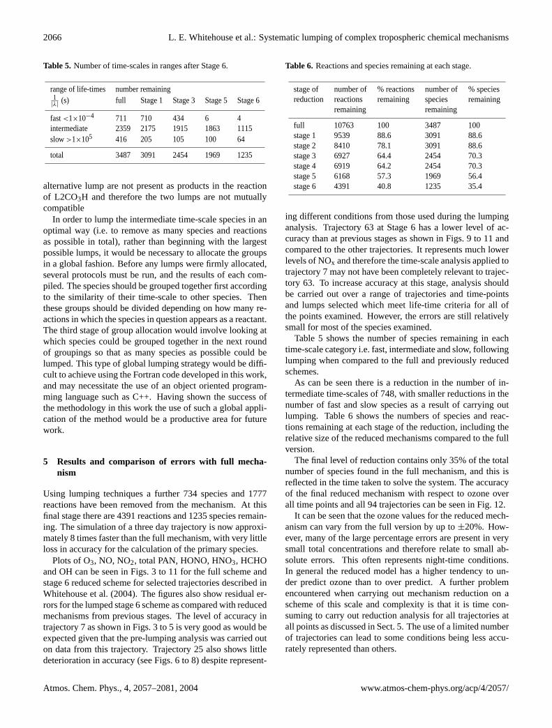
Table 5. Number of time-scales in ranges after Stage 6.

range of life-times number remaining1|λ|

(s) full Stage 1 Stage 3 Stage 5 Stage 6

fast<1×10−4 711 710 434 6 4intermediate 2359 2175 1915 1863 1115slow>1×105 416 205 105 100 64

total 3487 3091 2454 1969 1235

alternative lump are not present as products in the reactionof L2CO3H and therefore the two lumps are not mutuallycompatible

In order to lump the intermediate time-scale species in anoptimal way (i.e. to remove as many species and reactionsas possible in total), rather than beginning with the largestpossible lumps, it would be necessary to allocate the groupsin a global fashion. Before any lumps were firmly allocated,several protocols must be run, and the results of each com-piled. The species should be grouped together first accordingto the similarity of their time-scale to other species. Thenthese groups should be divided depending on how many re-actions in which the species in question appears as a reactant.The third stage of group allocation would involve looking atwhich species could be grouped together in the next roundof groupings so that as many species as possible could belumped. This type of global lumping strategy would be diffi-cult to achieve using the Fortran code developed in this work,and may necessitate the use of an object oriented program-ming language such as C++. Having shown the success ofthe methodology in this work the use of such a global appli-cation of the method would be a productive area for futurework.

5 Results and comparison of errors with full mecha-nism

Using lumping techniques a further 734 species and 1777reactions have been removed from the mechanism. At thisfinal stage there are 4391 reactions and 1235 species remain-ing. The simulation of a three day trajectory is now approxi-mately 8 times faster than the full mechanism, with very littleloss in accuracy for the calculation of the primary species.

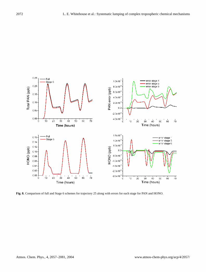
Plots of O3, NO, NO2, total PAN, HONO, HNO3, HCHOand OH can be seen in Figs.3 to 11 for the full scheme andstage 6 reduced scheme for selected trajectories described inWhitehouse et al.(2004). The figures also show residual er-rors for the lumped stage 6 scheme as compared with reducedmechanisms from previous stages. The level of accuracy intrajectory 7 as shown in Figs.3 to 5 is very good as would beexpected given that the pre-lumping analysis was carried outon data from this trajectory. Trajectory 25 also shows littledeterioration in accuracy (see Figs.6 to 8) despite represent-

Table 6. Reactions and species remaining at each stage.

stage of number of % reactions number of % speciesreduction reactions remaining species remaining

remaining remaining

full 10763 100 3487 100stage 1 9539 88.6 3091 88.6stage 2 8410 78.1 3091 88.6stage 3 6927 64.4 2454 70.3stage 4 6919 64.2 2454 70.3stage 5 6168 57.3 1969 56.4stage 6 4391 40.8 1235 35.4

ing different conditions from those used during the lumpinganalysis. Trajectory 63 at Stage 6 has a lower level of ac-curacy than at previous stages as shown in Figs.9 to 11 andcompared to the other trajectories. It represents much lowerlevels of NOx and therefore the time-scale analysis applied totrajectory 7 may not have been completely relevant to trajec-tory 63. To increase accuracy at this stage, analysis shouldbe carried out over a range of trajectories and time-pointsand lumps selected which meet life-time criteria for all ofthe points examined. However, the errors are still relativelysmall for most of the species examined.

Table 5 shows the number of species remaining in eachtime-scale category i.e. fast, intermediate and slow, followinglumping when compared to the full and previously reducedschemes.

As can be seen there is a reduction in the number of in-termediate time-scales of 748, with smaller reductions in thenumber of fast and slow species as a result of carrying outlumping. Table6 shows the numbers of species and reac-tions remaining at each stage of the reduction, including therelative size of the reduced mechanisms compared to the fullversion.

The final level of reduction contains only 35% of the totalnumber of species found in the full mechanism, and this isreflected in the time taken to solve the system. The accuracyof the final reduced mechanism with respect to ozone overall time points and all 94 trajectories can be seen in Fig. 12.

It can be seen that the ozone values for the reduced mech-anism can vary from the full version by up to±20%. How-ever, many of the large percentage errors are present in verysmall total concentrations and therefore relate to small ab-solute errors. This often represents night-time conditions.In general the reduced model has a higher tendency to un-der predict ozone than to over predict. A further problemencountered when carrying out mechanism reduction on ascheme of this scale and complexity is that it is time con-suming to carry out reduction analysis for all trajectories atall points as discussed in Sect.5. The use of a limited numberof trajectories can lead to some conditions being less accu-rately represented than others.


L. E. Whitehouse et al.: Systematic lumping of complex tropospheric chemical mechanisms 2067L. E. Whitehouse: Systematic Lumping of Complex Tropospheric Chemical Mechanisms 11

Fig. 3. Comparison of full and Stage 6 schemes for trajectory 7 along with errors for each stage for O3, NO and NO2.





Fig. 4. Comparison of full and Stage 6 schemes for trajectory 7 along with errors for each stage for OH, HCHO and HNO3.






Fig. 5. Comparison of full and Stage 6 schemes for trajectory 7 along with errors for each stage for PAN and HONO.

Fig. 12. Figure demonstrating the relationship between the ozone inthe full mechanism and the Stage 6 lumped mechanism. The upperred lines indicates a 10% variation above the full mechanism values,and the lower red line indicates a 20% variation below.

the Stage 6 reduction for all trajectories can be seen in Figure13.

Fig. 13. Figure demonstrating the relationship between the totalVOC in the full mechanism and the Stage 6 lumped mechanism.The red lines indicate a variation of 5% on either side of the fullmechanism values.

The total VOC values for the full mechanism and the Stage6 reduced mechanism are within 5% of each other. The fact





16 L. E. Whitehouse: Systematic Lumping of Complex Tropospheric Chemical Mechanisms


that none of the primary VOCs are removed from the mech-anism, and are also not lumped, contributes to this high levelof accuracy

The relationship between total NOx from the full mecha-nism and the Stage 6 reduction is shown in Figure 14. Thesevalues can be seen to lie within 10% of each other at all timesover all trajectories. As before the highest level of absoluteerror is at the high NOx conditions.

The relationship between OH predicted by the full mech-anism and the Stage 6 reduction is shown in Figure 15. TheOH is also well represented by the full scheme. OH and HO2

are strongly coupled at relatively high NOx concentrationsand so [OH] depends on the total rate of initiation which in-cludes not only O1D + H2O, but also O3 + alkenes and a widerange of carbonyl photolyses. In addition, OH loss includesnot only reaction with primary hydrocarbons, but also with awide range of secondary carbonyl compounds. The reducedmechanism clearly captures these processes well.

6 Discussion

Lumping techniques have been widely used as a method ofreducing the size of large chemical systems. Many previous

Fig. 14. Figure demonstrating the relationship between the totalNOx in the full mechanism and the Stage 6 lumped mechanism.The red lines indicate a variation of 10% on either side of the fullmechanism values.

techniques have concentrated on lumping primary VOCs andhave used a variety of non-formal techniques for establishinglumped rate coefficients. In order to lump the MCM, a moreformal approach was required in order to allow a higher level







Fig. 15. Figure demonstrating the relationship between OH pre-dicted by the full mechanism and the Stage 6 lumped mechanismacross all trajectories. The top red line indicates a variation of +12%and the bottom line a variation of −5%.

of automation than previous techniques have permitted. Thiswork has presented such a methodology based on the lump-ing of species with intermediate lifetimes and the allocationof product coefficients with respect to the ratio of the form-

ing species. Rate coefficients for the lumped reactions weretaken as the mean of the rate coefficients of contributing ele-mentary reactions in the case of inexact lumping. However,for groups of species with identical lifetimes lumping was ex-act. Using these techniques many lumps were identified, and,combined with other techniques such as sensitivity analysis,lumping allowed the size of the final reduced mechanism tobe about 50% of the size of the full mechanism in terms ofreactions and 35% in terms of species.

The lumping has been confined mainly to a few types ofspecies. The first large group are peracids, and the secondoxoacids. The third large group of species are nitrates, ap-pearing in L21NO3 to L43NO3. Other groups include per-oxy acyl nitrates (PANs), oxepins, carbonates and substitutedphenols. Each group of species was defined according tosimilarities in lifetimes and reaction structures. Lumped re-action rates were formed in general by using average reactionrates for the species reacting with OH.

The computational time necessary for a single trajectoryhas been reduced by a factor of 8. However, in order for thislumping to be carried out in an optimum fashion an “intelli-gent” program would be needed in order to divide groups se-lected using the flowchart system into sub-groups, such thata larger number of species could be lumped in total. In this












Fig. 12.Figure demonstrating the relationship between the ozone inthe full mechanism and the Stage 6 lumped mechanism. The upperred lines indicates a 10% variation above the full mechanism values,and the lower red line indicates a 20% variation below.









A plot of total VOC concentration over the three day pe-riod, as predicted by the full mechanism against those fromthe Stage 6 reduction for all trajectories can be seen inFig. 13.

The total VOC values for the full mechanism and the Stage6 reduced mechanism are within 5% of each other. The factthat none of the primary VOCs are removed from the mech-anism, and are also not lumped, contributes to this high levelof accuracy

The relationship between total NOx from the full mech-anism and the Stage 6 reduction is shown in Fig.14. Thesevalues can be seen to lie within 10% of each other at all times

16 L. E. Whitehouse: Systematic Lumping of Complex Tropospheric Chemical Mechanisms


that none of the primary VOCs are removed from the mech-anism, and are also not lumped, contributes to this high levelof accuracy

The relationship between total NOx from the full mecha-nism and the Stage 6 reduction is shown in Figure 14. Thesevalues can be seen to lie within 10% of each other at all timesover all trajectories. As before the highest level of absoluteerror is at the high NOx conditions.

The relationship between OH predicted by the full mech-anism and the Stage 6 reduction is shown in Figure 15. TheOH is also well represented by the full scheme. OH and HO2

are strongly coupled at relatively high NOx concentrationsand so [OH] depends on the total rate of initiation which in-cludes not only O1D + H2O, but also O3 + alkenes and a widerange of carbonyl photolyses. In addition, OH loss includesnot only reaction with primary hydrocarbons, but also with awide range of secondary carbonyl compounds. The reducedmechanism clearly captures these processes well.

6 Discussion

Lumping techniques have been widely used as a method ofreducing the size of large chemical systems. Many previous


techniques have concentrated on lumping primary VOCs andhave used a variety of non-formal techniques for establishinglumped rate coefficients. In order to lump the MCM, a moreformal approach was required in order to allow a higher level





Fig. 15. Figure demonstrating the relationship between OH pre-dicted by the full mechanism and the Stage 6 lumped mechanismacross all trajectories. The top red line indicates a variation of +12%and the bottom line a variation of −5%.

of automation than previous techniques have permitted. Thiswork has presented such a methodology based on the lump-ing of species with intermediate lifetimes and the allocationof product coefficients with respect to the ratio of the form-

ing species. Rate coefficients for the lumped reactions weretaken as the mean of the rate coefficients of contributing ele-mentary reactions in the case of inexact lumping. However,for groups of species with identical lifetimes lumping was ex-act. Using these techniques many lumps were identified, and,combined with other techniques such as sensitivity analysis,lumping allowed the size of the final reduced mechanism tobe about 50% of the size of the full mechanism in terms ofreactions and 35% in terms of species.


The computational time necessary for a single trajectoryhas been reduced by a factor of 8. However, in order for thislumping to be carried out in an optimum fashion an “intelli-gent” program would be needed in order to divide groups se-lected using the flowchart system into sub-groups, such thata larger number of species could be lumped in total. In this


Fig. 15. Figure demonstrating the relationship between OH pre-dicted by the full mechanism and the Stage 6 lumped mechanismacross all trajectories. The top red line indicates a variation of +12%and the bottom line a variation of−5%.

over all trajectories. As before the highest level of absoluteerror is at the high NOx conditions.

The relationship between OH predicted by the full mech-anism and the Stage 6 reduction is shown in Fig.15. TheOH is also well represented by the full scheme. OH and HO2are strongly coupled at relatively high NOx concentrationsand so [OH] depends on the total rate of initiation which in-cludes not only O1D+H2O, but also O3+alkenes and a widerange of carbonyl photolyses. In addition, OH loss includesnot only reaction with primary hydrocarbons, but also with awide range of secondary carbonyl compounds. The reducedmechanism clearly captures these processes well.



6 Discussion

Lumping techniques have been widely used as a method ofreducing the size of large chemical systems. Many previoustechniques have concentrated on lumping primary VOCs andhave used a variety of non-formal techniques for establishinglumped rate coefficients. In order to lump the MCM, a moreformal approach was required in order to allow a higher levelof automation than previous techniques have permitted. Thiswork has presented such a methodology based on the lump-ing of species with intermediate lifetimes and the allocationof product coefficients with respect to the ratio of the form-ing species. Rate coefficients for the lumped reactions weretaken as the mean of the rate coefficients of contributing ele-mentary reactions in the case of inexact lumping. However,for groups of species with identical lifetimes lumping was ex-act. Using these techniques many lumps were identified, and,combined with other techniques such as sensitivity analysis,lumping allowed the size of the final reduced mechanism tobe about 50% of the size of the full mechanism in terms ofreactions and 35% in terms of species.


The computational time necessary for a single trajectoryhas been reduced by a factor of 8. However, in order for thislumping to be carried out in an optimum fashion an “intelli-gent” program would be needed in order to divide groups se-lected using the flowchart system into sub-groups, such thata larger number of species could be lumped in total. In thisway larger continuous groups of reactions could be lumpedbefore redivision had to occur. Although the lumping car-ried out here is not complete, with some development thelumping strategy developed has the potential to significantlyfurther reduce the dimension and computational time of theMCM.

There are a number of advantages to executing lumping inthis manner rather than those discussed in the introduction.Within a complex mechanism such as the MCM, identify-ing species with similar lifetimes throughout the simulationis a useful starting point in terms of finding groups of speciesthat take part in the same reaction structures at similar ki-netic rates. Identifying species that play a similar role withinthe mechanism can therefore be determined from a formalbasis. Groups of species with similar lifetimes can be auto-matically found and then probed for similarities in terms oftheir reaction structures. The method is particularly success-ful for a mechanism like the MCM where large numbers ofintermediate compounds react via many parallel but similar

reaction paths. In addition, the techniques developed heredo not involve the lumping of primary compounds, makingit possible to easily alter the emission profiles which the re-duce mechanism represents. If primary VOCs are lumped asin many previous techniques, the whole mechanism must bereconstructed where emissions profiles change.

In a number of the lumping techniques discussed here, therate parameters of the lumped scheme are optimised in or-der to fit certain experimental data or full model simulations.This removes any possibility of automating the proceduresused. Also if the lumped model is to be accurate under con-ditions other than those for which the rate parameters are op-timised it is possible that re-optimisation of the parametersshould take place. In the present work, using lumped ratecoefficients based on rate parameters from the full schememeans that they can be calculated simply in an automatic pro-cedure and no further optimisation is necessary. The coeffi-cients for the products in a lumped reaction are taken from ra-tios of the rates of the reactions by which the lumped speciesis now produced. The new data files needed in order to storethis data can be generated by means of a simple Fortran rou-tine, and with minimal adaptations to the driver code thesecoefficients can be calculated at each step.

A further advantage is that because both forward and re-verse transformations have been defined here, it is possibleto track the concentrations of the original compounds if nec-essary. One possible limitation of the methods is the formof the expression used for calculating the coefficients for theproducts in the lumped reactions where,

σm =rate of formation of Sj

sum of rate of formation of all species in lumped group, (70)

andσm is the coefficient for themth product formed fromthe species Sj which has now been lumped, see Sect.4.2.2,Eq. (20). For this assumption to be valid, it was assumedthat the lumped species had the same initial conditions. Thiswas not a concern when applying it to the MCM as for thescenarios considered all intermediate species had zero initialconditions. However when considering the wider use of thismethod a further criterion when debating the suitability of aspecies for addition to a lump may be its initial value.

7 Conclusions

A formal method of species lumping which can be appliedautomatically to intermediate compounds within a detailedand complex tropospheric scheme has been developed. Themethod is based on grouping species with reference to theirlifetimes. Preliminary application to the MCMv2.0 has ledto the removal of 734 species and 1777 reactions from thescheme with minimal degredation of accuracy across a widerange of test trajectories. In combination with other reduc-tion techniques such as sensitivity analysis and the applica-tion of the QSSA, a final reduced mechanism has been de-veloped that contains 35.4% of the number of species and



40.8% the number of reactions compared to the full mech-anism. This has led to a speed up of a factor of 8 in termsof computer simulation time. Analysis of the errors obtainedby using the most reduced mechanism were determined tobe less than 5% for many of the trajectories studied, and lessthan 10% for the majority.

Improvements in the lumping strategy in order to increaseoptimality would require that the lumps be chosen in such away that a lumped species produces a single lumped productwhich is applicable for as many situations as possible. Thiswould eliminate the need for product coefficients to be calcu-lated from the rate coefficients at each time-point and wouldlead to much greater simplicity within the mechanism. Inorder to achieve this it would be necessary to allocate thegroups in a global fashion. Before any lumps are firmly al-located, several protocols should be run and the results of allcompiled. The species should be grouped according to thesimilarity of their lifetimes compared to the other species.It would then be necessary to establish if a secondary lumpcould be formed from the products of the lumped reactions ofthis group. Adjustments should then be made to the groupsto allow this to occur in an optimum way. Future work willinclude the development of an automatic approach to achiev-ing such an optimally lumped scheme.



Appendix 1

Table 7. Description of Lumped Groups for Acids, Nitrates, Oxepins and Substituted Phenols.

Lump Type of Compounds No. of Range of Lifetimes (s) Equivalent Reaction Rates Range of Reaction RatesName Species After 36 Hours (defined inPilling et al.(1999)) Species + OH

in Lump of Simulation (molecule cm−3)1−ms−1

L1CO3H peracids 59 1.08×104−8.10×104 J41 4.52×10−11

−3.7×10−12

L2CO3H peracids 42 9.35×102−1.31×104 J24, J41 5.44×10−10

−3.03×10−11

L3CO3H peracids 3 1.24×104−1.96×104 J15, J41 3.00×10−11

−1.47×10−11

L4CO3H peracids 7 1.48×104−5.29×104 J22, J41 3.05×10−11

−5.35×10−12

L5CO3H peracids 4 6.48×103−1.08×104 J18, J19, J41 6.90×10−11

−3.69×10−11

L6OOH oxoacids 3 7.57×104−8.25×104 J41 1.90×10−12e(190/T EMP)

−

2.20×10−12e(190/T EMP)

L7OOH oxoacids 86 2.50×103−8.24×104 J41 3.59×10−12

−2.42×10−10

L8OOH oxoacids 52 3.31×103−5.90×104 J22, J41 4.33×10−12

−1.42×101−0

L9OOH oxoacids 79 8.36×103−5.33×104 J15, J41, 3.44×102

−5.56×10−11

1.90×10−12e(190/T EMP)

L10OOH oxoacids 20 2.14×103−3.85×104 J22×2, J41 7.25×10−12

−9.61×10−11

L11OOH oxoacids 4 2.99×103−7.00×103 J15, J41 6.21×10−11

−1.61×10−10

L12OOH oxoacids 2 8.37×103−1.03×104 J24, J41 4.09×10−11

−5.26×10−11

L13OOH oxoacids 2 5.85×103−1.61×104 J24×2, J41 7.03×10−11

−7.26×10−11

L14OOH oxoacids 26 4.50×103−4.03×104 J22, J41, 4.83×10−12

−1.07×10−10

1.90×10−12e(190/T EMP)

L15OOH oxoacids 6 3.13×103−3.28×103 J22, J35, J41 1.99×10−11

−2.75×10−11

L16OOH oxoacids 9 6.95×103−8.19×103 J18×2, J22, J41 5.06×10−11

−6.19×10−11


−7.44×10−11


−1.37×10−10

L19OOH oxoacids 2 8.20×103−8.24×103 J15, J22×2, J41 4.75×10−11

−4.78×10−11

L20OOH oxoacids 3 4.90×103−5.11×103 J18, J19, J22, J41, 8.51×10−11

−8.94×10−11

1.90×10−12e(190/T EMP)

L21NO3 nitrates 16 1.13×105−5.90×105 4.57×10−13

−8.76×10−13

L22NO3 nitrates 9 9.55×104−1.35×105 J55 8.64×10−14

−1.68×10−12

L23NO3 nitrates 44 3.98×104−5.14×105 J53 2.26×10−13

−1.22×10−11

L25NO3 nitrates 15 1.39×105−2.86×105 J54 4.9×10−13

−2.7×10−12

L26NO3 nitrates 15 7.72×104−1.19×105 J54 3.02×10−12

−6.03×10−12

L27NO3 nitrates 2 6.93×104−7.04×104 J54 6.03×10−12

−6.15×10−12

L28NO3 nitrates 5 5.71×104−6.81×104 J54 6.28×10−12

−7.74×10−12

L29NO3 nitrates 3 4.99×104− 5.46×104 J54 8.15×10−12

−9.04×10−12

L30NO3 nitrates 8 3.42×104−4.41×104 J54 1.04×10−11

−1.36×10−11

L31NO3 nitrates 7 2.55×104−3.27×104 J54 1.38×10−11

−1.97×10−11

L32NO3 nitrates 11 6.61×104− 1.56×105 J22 1.50×10−12

− 6.08×10−12

L33NO3 nitrates 2 5.94×103−8.35×103 J53×2 6.04×10−11

−8.55×10−11

L34NO3 nitrates 3 2.31×104−1.29×105 J56, J57 5.23×10−13

−1.89×10−11

L35NO3 nitrates 7 9.37×104−1.48×105 J22, J53 9.64×10−13

−2.99×10−12

L36NO3 nitrates 2 6.25×103−1.48×104 J15, J55 2.21×10−12

−7.00×10−11

L37NO3 nitrates 11 7.59×103−9.10×103 J18×2, J22 4.70×10−11

−5.83×10−11

L38NO3 nitrates 8 7.00×103−8.26×103 J15, J24 4.70×10−11

−5.83×10−11

L39NO3 nitrates 2 3.13×103−3.65×103 J35, J55 5.01×10−12

−2.85×10−11

L40NO3 nitrates 3 3.75×104−5.17×104 J41, 3.74×10−12

−7.52×10−12

1.90×10−12e(190/T EMP)

L41NO3 nitrates 2 1.54×104−1.57×104 J15, J54 2.25×10−11

−2.33×10−11

L42NO3 nitrates 7 9.05×104−1.07×105 J22, J54 1.79×10−12

−2.65×10−12

L43PIN oxepins 15 1.32×103 J61, 1.00×1011, 1.00×10−10

L44PIN oxepins 12 4.39×103 1.00×1011, 1.00×10−10

L46PIN oxepins 4 4.45×103 9.20×1012, 1.00×10−10

L47S substituted phenols 8 6.31×103 8.20×1011



Table 8. Description of Lumped Groups for Peroxy Acyl Nitrates and Carbonates.

Lump Type of Compounds No. of Range of Lifetimes (s) Equivalent Reaction Rates Range of Reaction RatesName Species After 36 Hours (defined inPilling et al.(1999)) Species + OH

in Lump of Simulation (molecule cm−3)1−ms−1

PAN1 peroxy acyl nitrates 5 3.29×103 KBPAN×0.67, 1.06×1012

PAN2 peroxy acyl nitrates 3 2217.25−2217.27 KBPAN 1.15×10−13−5.15×10−13

PAN3 peroxy acyl nitrates 2 2217.25 KBPAN, 9.55×1013

PAN4 peroxy acyl nitrates 4 2217.24 KBPAN 1.15×1012−1.38×1012

PAN5 peroxy acyl nitrates 5 2217.18−2217.22 KBPAN 1.75×1012−3.17×1012

















L1CO3 carbonates 4 3.38×104 KAPNO, KFPAN, KAPHO2,1.6KRO2NO3

L2CO3 carbonates 10 3.38×104 KAPNO, KFPAN, KAPHO2,1.6KRO2NO3

Acknowledgements.The authors would like to thank the NERC forfinancial support and J. Toth for useful discussions.

Edited by: L. Carpenter

References

Campbell, S. L. and Meyer, C. D.: Generalized Inverses of LinearTransformations, Pitman, London, 1979.

Fish, D. J.: The automatic generation of reduced mechanisms fortropospheric chemistry modelling, Atm. Env., 34, 1563–1574,2000.

Gery, M. W., Whitten, G. Z.and Killus, J. P., and Dodge, M. C.: Aphotochemical kinetics mechanism for urban and regional scalecomputer modelling, J. Geophys. Res., 94 D10, 12 925–12 956,1989.

Hough, A. M.: An intercomparison of mechanisms for the pro-duction of photochemical oxidants, J. Geophys. Res., 93, 3789–3812, 1988.

Jenkin, M. E., Saunders, S. M., and Pilling, M. J.: The troposphericdegradation of volatile organic compounds :A protocol for mech-anism development, Atm. Env., 31, 81–104, 1997.

Jenkin, M. E., Saunders, S. M., Derwent, R. G., and Pilling, M. J.:Development of a reduced speciated VOC degradation mecha-nism for use in ozone models, Atm. Env., 36, 4725–4734, 2002.

Leone, J. A. and Seinfeld, J. H.: Comparative analysis of chem-ical reaction mechanisms for photochemical smog, Atm. Env.,10, 437–464, 1985.

Li, G. and Rabitz, H.: A general analysis of exact lumping in chem-ical kinetics, Chem. Eng. Sci., 14, 1413–1430, 1989.

Li, G. and Rabitz, H.: A general analysis of approximate lumpingin chemical kinetics, Chem. Eng. Sci., 45, 977–1002, 1990.

Makar, P. A. and Polavarapu, S. M.: Analytic solutions for gas-phase chemical mechanism compression, Atm. Env., 31, 1025–1039, 1997.

Makar, P. A., Stockwell, W. R., and Li, S. M.: Gas-phase mecha-nism compression strategies: treatment of reactions, Atm. Env.,30, 831–842, 1996.

Middleton, P., Stockwell, W. R., and Carter, W. P. L.: Aggregationof volatile organic compound emissions for regional modelling,Atm. Env., 6, 1107–1133, 1990.

Pilling, M. J., Saunders, S., Carslaw, N., Pascoe, S., Jenkin, M., andDerwent, D.: Master Chemical Mechanism,http://www.chem.leeds.ac.uk/Atmospheric/MCM/mcmproj.html, 1999.

Stockwell, W. R., Middleton, P., Chang, J. S., and Tang, X. Y.:The second generation regional acid deposition model mecha-


http://www.chem.leeds.ac.uk/Atmospheric/MCM/mcmproj.html

http://www.chem.leeds.ac.uk/Atmospheric/MCM/mcmproj.html


nism for regional air-quality modelling, J. Geophys. Res., 95,16 343–16 367, 1990.

Tomlin, A. S., Turanyi, T., and Pilling, M. J.: Autoignition andlow temperature combustion of hydrocarbons, chap. Mathemati-cal tools for construction, investigation and reduction of combus-tion mechanisms, Elesvier, Amsterdam., 1998.

Wang, S. W., Georgopoulos, P. G., Li, G., and Rabitz, H.: Con-densing complex atmospheric chemistry mechanisms – I. Thedirect constrained approximate lumping (DCAL) method applied

to alkane photochemistry, Env. Sci. Tech., 32, 2018–2024, 1998.Wei, J. and Kuo, J. C.: A lumping analysis in monomolecular reac-

tion systems, Ind. Eng. Chem. Fundam., 8, 114–133, 1969.Whitehouse, L. E., Tomlin, A. S., and Pilling, M. J.: Systematic

reduction of complex tropospheric chemical mechanisms, PartI: sensitivity and time-scale analyses, Atmos. Chem. Phys., 4,2025–2056, 2004,SRef-ID: 1680-7324/acp/2004-4-2025.


http://direct.sref.org/1680-7324/acp/2004-4-2025

and physics systematic reduction of complex tropospheric … · 2016-01-11 · ical reaction...

Documents