Control & Dynamical Systems

CA L T EC H

Invariant Manifolds,the Spatial 3-Body Problemand Space Mission Design

Shane D. RossControl and Dynamical Systems, Caltech

G. Gomez, W.S. Koon, M.W. Lo, J.E. Marsden, J. MasdemontOctober 17, 2001

Introduction

�Theme

� Using dynamical systems theory applied to 3- and 4-body problems for understanding solar system dynam-ics and identifying useful orbits for space missions.

2

Introduction

�Theme

� Using dynamical systems theory applied to 3- and 4-body problems for understanding solar system dynam-ics and identifying useful orbits for space missions.

�Current research importance

� Development of some NASA mission trajectories, suchas the recently launched Genesis Discovery Mission,and the upcoming Europa Orbiter Mission

2

Introduction

�Theme

� Using dynamical systems theory applied to 3- and 4-body problems for understanding solar system dynam-ics and identifying useful orbits for space missions.

�Current research importance

� Development of some NASA mission trajectories, suchas the recently launched Genesis Discovery Mission,and the upcoming Europa Orbiter Mission

� Of current astrophysical interest for understandingthe transport of solar system material (eg, how ejectafrom Mars gets to Earth, etc.)

2

Genesis Discovery Mission� Genesis will collect solar wind samples at the Sun-Earth

L1 and return them to Earth.

� It was the first mission designed start to finish usingdynamical systems theory.

0

500000

z (km)

-1E+06

0

1E+06

x (km)

-500000

0

500000

y (km)XY

Z

HaloOrbit

Transferto Halo

Earth

Moon'sOrbit

ReturnTrajectoryto Earth

Sun

3

Europa Orbiter Mission

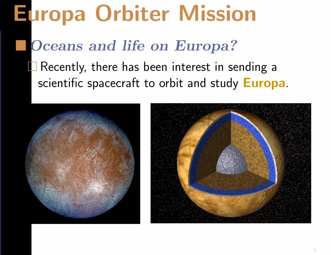
�Oceans and life on Europa?

� Recently, there has been interest in sending ascientific spacecraft to orbit and study Europa.

4

Europa Orbiter Mission

Europa Mission

5

Current Work� Goal: Find cheap way to Europa (consuming least amount

of fuel)

6

Current Work� Goal: Find cheap way to Europa (consuming least amount

of fuel)

• Flyby other bodies of interest along the way

6

Current Work� Goal: Find cheap way to Europa (consuming least amount

of fuel)

• Flyby other bodies of interest along the way

� Method: Take full advantage of the phase space struc-ture to yield optimal trajectory

6

Current Work� Goal: Find cheap way to Europa (consuming least amount

of fuel)

• Flyby other bodies of interest along the way

� Method: Take full advantage of the phase space struc-ture to yield optimal trajectory

� Model: Jupiter-Europa-Ganymede-spacecraft 4-bodymodel considered as two 3-body models

6

Current Work� Goal: Find cheap way to Europa (consuming least amount

of fuel)

• Flyby other bodies of interest along the way

� Method: Take full advantage of the phase space struc-ture to yield optimal trajectory

� Model: Jupiter-Europa-Ganymede-spacecraft 4-bodymodel considered as two 3-body models

• Extend previous work from planar model to 3D

6

History of 3-Body Problem

�Brief history:

� Founding of dynamical systems theory: Poincare [1890]

� Special orbits: Conley [1963,1968], McGehee [1969]

� Invariant manifolds: Simo, Llibre, and Martinez [1985], Gomez,

Jorba, Masdemont, and Simo [1991]

� Applied to space missions: Howell, Barden, and Lo [1997],

Lo and Ross [1997,1998] Koon, Lo, Marsden, and Ross [2000],

Gomez, Koon, Lo, Marsden, Masdemont, and Ross [2001]

� Using optimal control: Serban, Koon, Lo, Marsden, Petzold,

Ross, and Wilson [2001]

7

Three-Body Problem

�Circular restricted 3-body problem

� the two primary bodies move in circles; the muchsmaller third body moves in the gravitational field ofthe primaries, without affecting them

8

Three-Body Problem

�Circular restricted 3-body problem

� the two primary bodies move in circles; the muchsmaller third body moves in the gravitational field ofthe primaries, without affecting them

� the two primaries could be the Sun and Earth, theEarth and Moon, or Jupiter and Europa, etc.

� the smaller body could be a spacecraft or asteroid

8

Three-Body Problem

�Circular restricted 3-body problem

� the two primary bodies move in circles; the muchsmaller third body moves in the gravitational field ofthe primaries, without affecting them

� the two primaries could be the Sun and Earth, theEarth and Moon, or Jupiter and Europa, etc.

� the smaller body could be a spacecraft or asteroid

� we consider the planar and spatial problems

� there are five equilibrium points in the rotating frame,places of balance which generate interesting dynamics

8

Three-Body Problem• 3 unstable points on line joining two main bodies – L1, L2, L3

• 2 stable points at ±60◦ along the circular orbit – L4, L5

-1 -0.5 0 0.5 1

-1

-0.5

0

0.5

1

x (rotating frame)

y (r

otat

ing

fram

e)

mS = 1 -µ mE = µ

S E

Earth’s orbit

L2

L4

L5

L3 L1

spacecraft

Equilibrium points

9

Three-Body Problem� orbits exist around L1 and L2; both periodic and quasi-

periodic

• Lyapunov, halo and Lissajous orbits

� one can draw the invariant manifolds assoicated to L1

(and L2) and the orbits surrounding them

� these invariant manifolds play a key role in what follows

10

Three-Body Problem� Equations of motion:

x− 2y = −U effx , y + 2x = −U eff

y

where

U eff = −(x2 + y2)

2− 1− µ

r1− µ

r2.

� Have a first integral, the Hamiltonian energy, given by

E(x, y, x, y) =1

2(x2 + y2) + U eff(x, y).

11

Three-Body Problem� Equations of motion:

x− 2y = −U effx , y + 2x = −U eff

y

where

U eff = −(x2 + y2)

2− 1− µ

r1− µ

r2.

� Have a first integral, the Hamiltonian energy, given by

E(x, y, x, y) =1

2(x2 + y2) + U eff(x, y).

� Energy manifolds are 3-dimensional surfaces foliatingthe 4-dimensional phase space.

� This is for the planar problem, but the spatial problemis similar.

11

Regions of Possible Motion

�Effective potential

� In a rotating frame, the equations of motion describea particle moving in an effective potential plus a mag-netic field (goes back to work of Jacobi, Hill, etc).

Ueff

S JL1 L2

ExteriorRegion (X)

Interior (Sun) Region (S)

JupiterRegion (J)

ForbiddenRegion

Effective potential Level set shows accessible regions

12

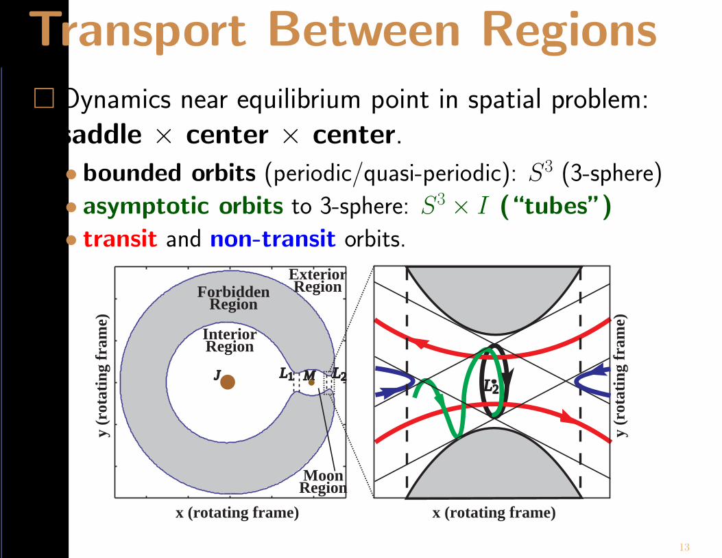
Transport Between Regions� Dynamics near equilibrium point in spatial problem:

saddle × center × center.• bounded orbits (periodic/quasi-periodic): S3 (3-sphere)

• asymptotic orbits to 3-sphere: S3 × I (“tubes”)

• transit and non-transit orbits.

x (rotating frame)

y (r

otat

ing

fram

e)

J ML1

x (rotating frame)

y (r

otat

ing

fram

e)

L2

ExteriorRegion

InteriorRegion

MoonRegion

ForbiddenRegion

L2

13

Transport Between Regions� Asymptotic orbits form 4D invariant manifold tubes

(S3 × I) in 5D energy surface.

� red = unstable, green = stable

0.820.84

0.860.88

0.90.92

0.940.96

0.981

1.02−0.02

0

0.02

0.04

0.06

0.08

0.1−0.010

0.01

x

z

y

14

Transport Between Regions• These manifold tubes play an important role in governing what

orbits approach or depart from a moon (transit orbits)

• and orbits which do not (non-transit orbits)

• transit possible for objects “inside” the tube, otherwise notransit — this is important for transport issues

x (rotating frame)

y (r

ota

tin

g fra

me

)

Passes throughL2 Equilib r ium Region

JupiterEuropa

L2

Ends inCaptureAround Moon

SpacecraftBegins

Inside Tube

15

Transport Between Regions• Transit orbits can be found using a Poincare section transver-

sal to a tube.

PoincareSection

Tube

16

Construction of Trajectories� One can systematically construct new trajectories, which

use little fuel.

• by linking stable and unstable manifold tubes in the right order

• and using Poincare sections to find trajectories “inside” thetubes

� One can construct trajectories involving multiple 3-bodysystems.

17

Construction of Trajectories• For a single 3-body system, we wish to link invariant manifold

tubes to construct an orbit with a desired itinerary

• Construction of (X ; M, I) orbit.

X

I ML1 L2

M

U3

U2U1U4

U3

U2

The tubes connecting the X,M , and I regions.

18

Construction of Trajectories• First, integrate two tubes until they pierce a common Poincaresection transversal to both tubes.

PoincareSection

Tube A

Tube B

19

Construction of Trajectories• Second, pick a point in the region of intersection and integrate

it forward and backward.

PoincareSection

Tube A

Tube B

20

Construction of Trajectories•Planar: tubes (S × I) separate transit/non-transit orbits.

•Red curve (S1) (Poincare cut of L2 unstable manifold.Green curve (S1) (Poincare cut of L1 stable manifold.

• Any point inside the intersection region ∆M is a (X ; M, I) orbit.

∆M = (X;M,I)

Intersection Region

0.92 0.94 0.96 0.98 1 1.02 1.04 1.06 1.08

-0.08

-0.06

-0.04

-0.02

0

0.02

0.04

0.06

0.08

x (Jupiter-Moon rotating frame)

y (J

upite

r-M

oon

rota

ting

fram

e)

ML1 L2

0.01 0.015 0.02 0.025 0.03 0.035 0.04 0.045 0.05

-0.06

-0.04

-0.02

0

0.02

0.04

0.06

y (Jupiter-Moon rotating frame)

(X;M)

(;M,I)

y (J

upite

r-M

oon

rota

ting

fram

e).

Forbidden Region

Forbidden Region

StableManifold

UnstableManifold

StableManifold Cut

UnstableManifold Cut

Tubes intersect in position Poincare section of intersection21

Construction of Trajectories• Spatial: Invariant manifold tubes (S3 × I)

• Poincare cut is a topological 3-sphere S3 in R4.

◦ S3 looks like disk × disk: ξ2 + ξ2 + η2 + η2 = r2 = r2ξ + r2

η

• If z = c, z = 0, its projection on (y, y) plane is a curve.

• For unstable manifold: any point inside this curve is a (X ; M)orbit.

-0.005 0.0050

z

0.6

0.4

0.2

-0.2

0

-0.6

-0.4

z.

0 0.0100.005

y0.015

0.6

0.4

0.2

-0.2

0

-0.6

-0.4

y.

γz’z’. (z’,z’).

(y, y) Plane (z, z) Plane22

Construction of Trajectories• Similarly, while the cut of the stable manifold tube is S3, its

projection on (y, y) plane is a curve for z = c, z = 0.

• Any point inside this curve is a (M, I) orbit.

• Hence, any point inside the intersection region ∆M is a(X ; M, I) orbit.

-0.005 0.0050

z

0.6

0.4

0.2

-0.2

0

-0.6

-0.4

z.

0 0.0100.005

y0.015

0.6

0.4

0.2

-0.2

0

-0.6

-0.4

y.

C+s11

C+u21

C+s11C+u2

1

0.004 0.006 0.008 0.010 0.012 0.014

−0.01

−0.005

0

0.005

0.01

y

y.

γz'z'.1

γz'z'.2

Initial conditioncorresponding toitinerary (X;M,I)

(y, y) Plane (z, z) Plane Intersection Region

23

Construction of Trajectories

0.96 0.98 1 1.02 1.04-0.04

-0.02

0

0.02

0.04

x

y

0.96 0.98 1 1.02 1.04-0.04

-0.02

0

0.02

0.04

x

z

-0.005 0 0.005 0.010 0.015 0.020

-0.010

-0.005

0

0.005

y

z

z

0.981

1.021.04

-0.04-0.02

00.02

0.04-0.04

-0.02

0

0.02

0.04

xy

0.96

Construction of an (X,M, I) orbit24

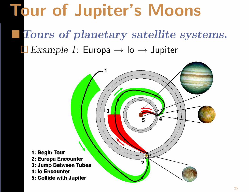
Tour of Jupiter’s Moons

�Tours of planetary satellite systems.

� Example 1: Europa → Io → Jupiter

25

Tour of Jupiter’s Moons� Example 2: Ganymede → Europa → injection into

Europa orbitGanymede's orbit

Jupiter

0.98

0.99

1

1.01

1.02

-0.02

-0.01

0

0.01

0.02

-0.02

-0.015

-0.01

-0.005

0

0.005

0.01

0.015

0.02

xy

z

0.990.995

11.005

1.01 -0.01

-0.005

0

0.005

0.01

-0.01

-0.005

0

0.005

0.01

yx

z

Close approachto Ganymede

Injection intohigh inclination

orbit around Europa

Europa's orbit

(a)

(b) (c)

-1. 5-1

-0. 50

0.51

1.5

-1. 5

-1

-0. 5

0

0.5

1

1.5

x

y

z

Maneuverperformed

26

Tour of Jupiter’s Moons

pgt-3d-orbit-eu.qt

27

Tour of Jupiter’s Moons• The Petit Grand Tour can be constructed as follows:

◦ Approximate 4-body system as 2 nested 3-body systems.

◦ Choose an appropriate Poinare section.

◦ Link the invariant manifold tubes in the proper order.

◦ Integrate initial condition (patch point) in the 4-body model.

Jupiter Europa

Ganymede

Spacecrafttransfer

trajectory

∆V at transferpatch point

-1. 5 -1. 4 -1. 3 -1. 2 -1. 1 -1

-0.08

-0.06

-0.04

-0.02

0

0.02

0.04

0.06

0.08

0.1

0.12

x (Jupiter-Europa rotating frame)

x (J

upite

r-E

urop

a ro

tatin

g fr

ame)

.

Gan γzz.1 Eur γzz.

2

Transferpatch point

Look for intersection of tubes Poincare section at intersection

28

Further Work

�More refinement needed

29

Further Work

�More refinement needed

� Control over inclination of final orbit

29

Further Work

�More refinement needed

� Control over inclination of final orbit

� Further reduce fuel cost using other techniques• Resonance transition to pump down orbit via repeated close

approaches to the moons

Using resonance transition to pump down orbit29

Further Work

Semimajor axis

Arg

umen

t of

peri

helio

n (d

egre

es)

Unstable manifold of P1Stable manifold of P1

Resonance region of P1

Unstable periodic orbit P1 Unstable periodic orbit P2

Resonance region of P2

(a)

(b) A stable island for the resonance region of P2

}} }

Overlapping region

Resonance transition as shown by Poincare map30

Further Work• Use low (continuous) thrust, rather than impulsive

• Combine with optimal control software (e.g., NTG, COOPT)

31

References• Gomez, G., W.S. Koon, M.W. Lo, J.E. Marsden, J. Masdemont and S.D. Ross

[2001] Invariant manifolds, the spatial three-body problem and spacemission design. AAS/AIAA Astrodynamics Specialist Conference.

• Koon, W.S., M.W. Lo, J.E. Marsden and S.D. Ross [2001] Resonance andcapture of Jupiter comets. Celestial Mechanics and Dynamical Astronomy,to appear.

• Koon, W.S., M.W. Lo, J.E. Marsden and S.D. Ross [2001] Low energy trans-fer to the Moon. Celestial Mechanics and Dynamical Astronomy. to appear.

• Serban, R., Koon, W.S., M.W. Lo, J.E. Marsden, L.R. Petzold, S.D. Ross,and R.S. Wilson [2001] Halo orbit mission correction maneuvers usingoptimal control. Automatica, to appear.

• Koon, W.S., M.W. Lo, J.E. Marsden and S.D. Ross [2000] Heteroclinic con-nections between periodic orbits and resonance transitions in celes-tial mechanics. Chaos 10(2), 427–469.

The End

32