and the last shall be first - mit

And the Last Shall be First:Federalism and Fiscal Outcomes in Germany

Jonathan RoddenMIT

Department of Political ScienceE53-433

77 Massachusetts AvenueCambridge, MA 02139

[email protected]

Original Draft:November 1998

This Draft:October 2, 2001

This paper explores the political economy of fiscal policy in the German Länder, testing severaltheories from the cross-national literature on budget deficits along with some additionalhypotheses relating to the incentives created by the German federal system. The results suggestthat governments controlled by the left spend and borrow more in the long run than right-winggovernments, though short-term partisan differences in fiscal management cannot be identified.Furthermore, incumbents spend and borrow more during election campaigns, and contrary tocommon wisdom, Land fiscal policy is decisively pro-cyclical. The most striking findings haveto do with Germany’s peculiar system of intergovernmental grants. Although transfers have apositive effect on fiscal balance in the short term, states increase expenditures and deficits in thelong run as they grow more dependent on transfers. The results may have implications for otherfiscal systems where lower-level governments have wide-ranging expenditure and borrowingautonomy but little authority to tax.

Draft prepared for presentation at Harvard UniversityOctober 10, 2001

The author wishes to thank Geoffrey Garrett, Jürgen von Hagen, Ronald Kneebone, Jorn Rattso,Helmut Seitz, and David Samuels for helpful comments on a previous draft.

mailto:[email protected]

2

I. Introduction

The growth of budget deficits and debt levels around the world has been the subject of

numerous theoretical and empirical investigations over the last twenty years. While progress has

been made in understanding the political, institutional, and economic underpinnings of budget

deficits at the central government level, very little attention has been given to the rapid growth of

deficits and debt at lower levels of government, even though subnational deficits have introduced

serious problems in a growing number of OECD, developing, and transition countries around the

world (Rodden, Eskeland, and Litvack 2001). In fact, by ignoring the effects of

intergovernmental relations and subnational fiscal decisions, existing studies of macroeconomic

management may miss an important source of cross-national variation; state and local deficits

often spill over to the central level, especially when the central government must provide bailouts

to profligate subnational entities.1

The comparative political economy of fiscal decision-making at subnational levels has

been virgin territory until recently. Most of the existing empirical work has been done on the

American states,2 though the U.S. is not a good case from which to build a general theory of

subnational fiscal behavior. In comparative perspective, the United States is an outlier in at least

two important respects. First of all, the American states very rarely run budget deficits. The

United States is the only major federation in the world in which the state/provincial sector was,

on average, in surplus during the 1980s and 1990s. Germany is a much more typical case; the

Länder (federal states) on average ran deficits amounting to 8 percent of revenue during this

period. Second, the US states are relatively self-reliant when compared with subnational units in

other federal countries, and while the vast majority of the grants received by the US states are

earmarked for specific purposes, most other federations resemble Germany’s more heavy reliance

on revenue sharing and equalization transfers.3

Fortunately, scholars have recently made progress towards a more nuanced understanding

of the varieties of fiscal and political federalism. For example, studies by Rattso (1999, 2000)

1 The experiences of Argentina and Brazil in the late 1980s have been particularly dramatic examples (Dillenger andWebb, 2000). See also Fornasari, Webb, and Zou (1998) and Treisman (2001) showing that subnational deficitslead to deficits at the central level.2 Inman (1997), Bohn and Inman (1996), Poterba (1994, 1996), Alt and Lowry (1994), Alt, Lowry, and Ferree(1996), Alesina and Bayoumi (1996), Eichengreen and Bayoumi (1995), Gramlich (1991), Holtz-Eakin and Rosen(1993).

3

examine incentives and fiscal decision-making in Norway, where local governments preside over

a large share of total public expenditures, but possess very limited taxing, borrowing, and

expenditure autonomy—perhaps the opposite end of the spectrum from the United States. Most

modern federations fall somewhere in the middle between the American and Norwegian

extremes. In Germany, as well as Argentina, Australia, Brazil, India, Spain, Mexico, South

Africa, and several other federations, provinces are responsible for important public functions

and highly dependent on intergovernmental transfers, but unlike unitary systems like Norway,

they face few centrally imposed limitations on expenditures and borrowing. Serious concerns

have been raised about moral hazard and overspending among subnational governments in such

systems.4

This paper seeks to contribute to this burgeoning comparative literature by using time

series cross-section analysis of fiscal outcomes in the German Länder to examine hypotheses

about the incentives created by fiscal and political institutions. Its primary objective is to

examine the incentive effects of intergovernmental transfers in a system with extremely limited

local tax authority but unlimited borrowing authority. The findings might have important

implications for some of the other federations listed above. Previous empirical studies of fiscal

outcomes in the Länder have relied on single-year snapshots (Wagschal 1996) or focused

exclusively on partisanship and counter-cyclical stabilization (Seitz 2000).

Second, this paper tests a variety of more general theories about the economic and

political sources of deficits that have heretofore been tested almost exclusively at the central

government level (See, e.g. Franzese1996, Roubini and Sachs 1989a, 1989b; Alesina and Perotti

1995). The advantages of cross-province over cross-national analysis are substantial; the

German Länder demonstrate useful variation over time and across units on several interesting

variables, but many of the usual concerns about institutional and cultural comparability—not to

mention data collection standards—are resolved by design.

Above all, this paper argues and demonstrates that transfer-dependence is an important

factor shaping Land-level fiscal outcomes. In the short term, Land-level fiscal outcomes are

extremely sensitive to fluctuations in intergovernmental transfers. In the long run, the perverse

incentives created by the German equalization system lead to a strong relationship between

3 The United States, Canada, and Switzerland are in a class by themselves among modern federations with respect torevenue autonomy (Rodden 2001).

4

transfer-dependence and deficits. Contrary to common wisdom, the Länder do not appear to

conduct counter-cyclical fiscal policy; if anything, the evidence suggests pro-cyclicality. Partisan

differences in short-term fiscal management cannot be identified, but in the long term, Länder

controlled by the Social Democrats run larger deficits than those controlled by the Christian

Democrats. Additionally, support is found for the hypothesis that incumbent politicians run

larger deficits during election campaigns. Long-term deficits are also smallest in the largest

states.

The second section introduces data on deficits and debt in the German Länder, and the

third section provides a brief overview of the German federal system. The fourth section lays out

several hypotheses that might explain cross-section and diachronic variation in deficits, explains

how each may be relevant in the German subnational context, and explains the operationalization

of each variable. Section five explains the empirical approach, section six provides results, and

the final section concludes.

II. The Problem: Deficits in the German Länder

Although the German federal government is famous for its prudent post-war fiscal

management, potentially serious problems at the Land level have been brewing for some time.

Recently, in the wake of debt servicing crises, court cases, and bailouts of two troubles Länder,

along with rapidly growing debt in Berlin and the new Eastern Länder, the perception of crisis is

growing, and reform of the intergovernmental system is a hot topic among German politicians,

policy analysis, and pundits.

Since the founding of the Bonn Republic, the Länder have taken on a sizable share of

total borrowing. By the end of 1996, the federal government’s debt reached 24 percent of GDP,

while the Länder stood at 16 percent, with the local governments at around 6 percent. Table 1

presents average deficit/revenue ratios for each of the Länder from 1992 to 1995, along with debt

per capita at the end of 1996.5 It shows that budgets are essentially balanced and debt per capita

4 Collections of qualitative case studies can be found in Rodden et al (2001) and von Hagen et al (2000).Quantitative studies include Jones et al (2000), Remmer and Wibbels (2000), and Bevilaqua (1999).5 Berlin is excluded from this and all following tables and charts because of its special status in the federation priorto unification, and the difficulty of aggregating data from East and West Berlin in the early 1990s.

5

is quite low in states like Bayern and Baden-Wuerttemberg, but they are three times as high in

troubled states like Bremen and Saarland. Table 1 also shows that average deficit levels in the

new Länder in their first years of existence have been between ten and thirty percent of revenue,

and in only a few years their per capita debt levels have reached those of their western

counterparts. These developments have been a cause of great concern in the German policy

community (see, e.g. Sachverständigenrat 1997). The independent fiscal management of the

Länder and the recent growth of subnational debt complicate macroeconomic management and

may even cause Germany to run afoul of the Maastricht criteria that overall deficits and debts not

exceed 3 and 60 percent (respectively) of GDP.

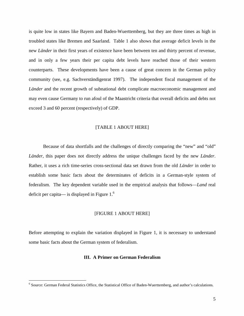
[TABLE 1 ABOUT HERE]

Because of data shortfalls and the challenges of directly comparing the “new” and “old”

Länder, this paper does not directly address the unique challenges faced by the new Länder.

Rather, it uses a rich time-series cross-sectional data set drawn from the old Länder in order to

establish some basic facts about the determinates of deficits in a German-style system of

federalism. The key dependent variable used in the empirical analysis that follows—Land real

deficit per capita— is displayed in Figure 1.6

[FIGURE 1 ABOUT HERE]

Before attempting to explain the variation displayed in Figure 1, it is necessary to understand

some basic facts about the German system of federalism.

III. A Primer on German Federalism

6 Source: German Federal Statistics Office, the Statistical Office of Baden-Wuerttemberg, and author’s calculations.

6

Administrative Federalism

It is not possible to provide a complete overview of the German federal system here, but

the key characteristics of the system motivating this paper can be easily summarized.7 First of

all, the Bund (central government) and the Länder are extremely interdependent. The Länder are

important veto players in the central government’s policy-making process—their governments

directly appoint the members of the Bundesrat (federal council), which must approve most

federal legislation. Moreover, the central government relies on the Land administrations for the

implementation of most of its policies—a model often referred to as "administrative federalism.”

The central government has very little bureaucratic capacity of its own, and much of the Land-

level administrative apparatus is specialized to implement policies that are made at the central

level. As a result, the Länder and Gemeinden (local governments) are responsible for a large

share (around 63 percent in 1995) of total expenditures. Given this structural interdependence of

Bund, Länder, and Gemeinden, it is very difficult for any government to achieve its goals without

bargaining, cajoling, or cooperating with one or two additional levels.

Fiscal Federalism

Multilateral bargaining between the interdependent Bund and Länder is also the modus

operandus in the collection and distribution of revenue. All of the most important taxes—the

income tax, corporation tax, and VAT, which together account for over three quarters of total tax

revenue—accrue to the federal and state governments jointly. Most decisions about the tax base

and rates are made by the federal government (subject to the approval of the Bundesrat) and for

the major taxes, collection is done by the revenue authorities of the Länder, which act as agents

of the federation under uniform federal guidelines. The significance of taxes assigned directly to

individual layers of government is low.

The vertical distribution of the shared taxes between Bund and Länder is very stable over

time because the actual percentage shares are laid out in the Constitution and can only be

changed by amendment. In order to ensure that the Länder receive sufficient funds to fulfill their

federally-mandated responsibilities in the face of changing fiscal circumstances, the vertical

7 For more detailed overviews, see Seitz (2000), Spahn and Foettinger (1997).

7

distribution of the VAT is frequently renegotiated between the Bund and the Länder. The

resulting bargain must be approved by the Länder in the Bundesrat. The constitution mandates

the maintenance of “equivalent living conditions” across the Länder, and to this end, the fiscal

equalization system goes to great lengths to redistribute revenue from the wealthy to the poor

Länder. First of all, the primary system of tax sharing distributes the proceeds of the major

shared taxes to the states as follows: income tax revenue is apportioned to the states according to

the derivation principle, corporate tax revenue is divided according to a formula based on plant

location, and a portion of the VAT is distributed to the states on a per capita basis. Next, the

secondary system of revenue equalization proceeds in three stages.

In the first stage, up to 25 percent of the VAT is redistributed to the Länder with the

lowest revenue after the primary tax sharing receipts are calculated. After this stage of

redistribution, the financial endowment (Finanzkraft) of each state is calculated and compared

with its financial needs (Finanzbedarf). Then at the second stage of equalization, revenue is

redistributed from states whose endowments exceed their needs, to those for whom the opposite

is true. The concept of "need" is based on the per capita tax income for the entire country. At

this stage, the weaker (Finanzschwach) states reach 95 of their financial "needs."

In the third stage of the equalization system, the federal government steps in to lift the

recipient states up to at least 99.5 percent of their "needs." It does this with supplementary

grants. At this stage, the Bund also bestows additional supplementary grants on some states to

compensate them for “special burdens.” Special supplementary grants are also received by

smaller Länder to compensate them for higher administrative costs, and recently, by some of the

"old" (pre-unification) Länder to compensate them for the higher fiscal burden they must bear

because of reunification. Massive supplementary transfers are also currently being made to the

East German Länder, and to provide bail-outs to Bremen and Saarland because of their debt

servicing obligations. After equalization and other transfers, the Länder with the lowest initial

per capita fiscal capacity— Bremen, Saarland, and the eastern Länder—end up with the highest

fiscal capacity per capita. Meanwhile, the Länder with the highest initial fiscal capacity—

Hamburg, Hesse, and Baden-Württemberg— end up with the lowest capacity after transfers

(Spahn and Föttinger, 1997).8

8 This section describes the key features of the equalization system during the period under analysis, but in June of2001, the federal government and Länder agreed to reforms that will be discussed in greater detail below.

8

Figure 2 summarizes the revenue sources of the Länder. Only nine percent of total

revenue comes from taxes over which the Länder have exclusive jurisdiction (primarily business

taxes), while 63 percent come from the various shared taxes. Fifteen percent of revenue comes

from other intergovernmental transfers. These include the supplementary grants made at the final

stage of the equalization process, along with transfers associated with joint federal-state

infrastructure programs. The revenue from shared taxes is highly predictable and completely

removed from the central government’s discretion. In comparison, the grants are quite

discretionary and can change substantially from year to year, often in ways that cannot be

predicted by Land budget planners.

Figure 2:

Sources of Revenue in the German Länder, 1995 (in % of total Land Revenue)

Shared taxes, 63%

Exclusive taxes, 9%

General-purpose grants, 6%

Specific-purpse grants, 9%

Other Revenue, 13%

Source: Spahn and Foettinger (1997).

Finally, the central government has no power to place numeric restrictions on the

borrowing activities of the Länder. Nor must the borrowing decisions of the Länder be approved

or reviewed by the Bund. Like the federal government, however, the Länder have their own

constitutional and statutory provisions that restrict them from borrowing more than the outlays

for investment purposes projected in the budget. These so-called golden rule provisions at the

Land level, however, have a number of well-known loopholes. Above all, "investment purposes"

is an extremely slippery concept, and it is not difficult to recast a variety of expenditures as

investment outlays, and since 1969 the constitutions of the Länder have allowed them to break

the “golden rule” in cases of “disturbances of general economic equilibrium.” Moreover,

Bremen and Saarland have chosen to simply ignore these constitutional provisions.

9

Because the Länder lack revenue autonomy, creditors clearly do not view them as fiscal

“sovereigns.” Despite widely divergent fiscal outcomes and debt servicing capacity, all of the

Länder have similar triple-A credit ratings from major credit rating agencies, which are explicitly

justified on the basis of the central government’s fiscal health and the belief that its constitutional

obligation to insure “equivalent living conditions” would prevent it from allowing any state to

default (see Rodden 2001).

Political Federalism

Germany’s intertwined form of federalism characterizes not only finance and

administration, but politics as well. Since Land elections are also elections for the federal upper

house, they have taken on the character of federal mid-term elections. They are fights on national

issues between national parties (with the exception of the Bavarian CSU), and are often viewed

as referenda on the popularity of the federal Chancellor and his government (Lohmann, Brady,

and Rivers 1997). Thus the electoral fates of Land-level politicians are driven largely by the

federation-wide value of their party labels. Many Land-level politicians have aspirations in

national politics, and careers often move back and forth between levels. In fact, virtually every

modern federal Chancellor has served as a Land Chancellor. Thus while politicians in the

Länder certainly face incentives to fiercely protect the interests of their state, they may

sometimes face incentives to be concerned with issues that transcend the interests of their

constituents.

IV. Fiscal Management in an Intertwined Federation: Hypotheses

In short, the German Länder have some discretion over a wide range of expenditures,

along with all budgetary and borrowing decisions, but have very little authority to raise revenue.

As a result, creditors and perhaps even voters do not always see Land officials as sovereign over

their own finances, but as pieces of a complex intertwined system. This may create a unique set

of incentives for Land level fiscal decision-makers, some of which differ from commonly-held

baseline assumptions about public finance, and some of which are undeniably perverse.

10

A. Equalization and Grants

The common resource allegory captures an overarching problem. The system described

above might turn public resources into a common pool that Land officials systematically over-

fish. First of all, since the individual Länder bear most of the costs of tax administration and only

a small fraction of additional tax revenues accrue to them, they face weak incentives to

strengthen audits and improve revenue collection (OECD 1998, Sachverständigenrat 1998, Von

Hagen and Hepp 2000). Fiscal discipline presents a potentially more serious problem if voters

and creditors believe that the central government or the other Länder are constitutionally

obligated to bail them out in the event of a debt-servicing crisis. Bailout expectations have

ultimately been confirmed. Beginning in 1987, Bremen and Saarland started to receive

supplementary transfers explicitly aimed at coping with high public debt. The expectations were

confirmed more explicitly in 1992 when the Constitutional Court handed down its decision

stipulating that the Bund must make extra transfers to Bremen and Saarland amounting to around

30 billion DM over the period from 1994-2000 in order to reduce public debt without severe

expenditure cuts (Seitz 1998). It now appears that the city-state of Berlin will soon request

similar bailout transfers.

Given these incentives, one might expect that throughout the post-war period, all of the

Länder will have persistently spent and borrowed beyond their means and avoided politically

painful expenditure cuts during lengthy downturns in the expectation of eventual federal bailouts.

However, this has clearly not been the case. Bailout expectations are more rational in some

Länder than others. Bailout expectations do not stem from the first two stages of equalization

between the Länder, but rather from the third stage at which the central government distributes

supplementary transfers. These transfers are clearly discretionary, and represent a ready-made

mechanism through which bailouts might be distributed. Bailout expectations are more rational

in the states that receive the largest transfers. Creditors and voters are aware that local debt

burdens cannot result in defaults, school closures, the firing of public employees and the like, and

fiscal decision-makers can hope that growing debt burdens will be covered by more generous

transfers in future years. For instance, when faced with a long-term decline in revenues that

requires politically painful expenditure cuts, the temptation to avoid adjustment might be strong

in the most transfer-dependent states. After all, these states are relatively poor and a relatively

11

large share of local expenditures are funded by non-residents. If local politicians choose to avoid

or post-pone fiscal adjustment and maintain current expenditure levels by increasing borrowing,

there are few reasons for local voters or creditors to punish them. They can claim with

considerable credibility that their fiscal burdens are ultimately not their responsibility. At the

other end of the spectrum, the states that pay into the equalization system and receive relatively

few transfers cannot credibly make such claims when faced with similar downturns. If they

overspend and run into debt servicing difficulties, there is no reason to believe that the federation

will step in with extra support.

H1: In the long term, transfer-dependence is associated with larger deficits.

A similar hypothesis has been examined in a cross-national study by Rodden (2001) and

studies of Argentina by Remmer and Wibbels (2000) and Jones et al (2000). It is related to the

vast public economics literatures on “fiscal illusion” and the “flypaper effect.” The basic

supposition in these studies is that voters and policy-makers view grants and locally-raised

revenues differently, and demand more of the former because they are perceived as “windfalls”

funded by others. The “flypaper” literature shows that increases in transfers stimulate much

more spending than would increases in local income.9 H1 suggests that in the long term,

increasing dependence on transfers will also stimulate deficits in Germany since they encourage

the perception not only that current expenditures are funded directly by transfers from residents

of other Länder, but also the perception that current deficits must ultimately be funded by future

non-residents.

Note that short-term fluctuations in transfers might have a very different effect than long-

term developments. A sustained, long-term increase in transfers might dilute incentives for fiscal

discipline, while a single-year increase in transfers might, if anything, lead to a smaller deficit (or

larger surplus), especially since transfers are more discretionary and difficult for budget

forecasters to predict than other forms of revenue. Thus it is important to use an estimation

technique that distinguishes between short-term and long-term changes.


9 For a review, see Hines and Thaler (1997).

12

Figure 3 illuminates trends and inter-state differences in real intergovernmental grants per

capita.10 It shows that transfers are relatively low and growth is minimal in the three wealthiest

states—Bayern, Hessen, and Nordrhein-Westfallen— and demonstrates a gentle upward trend in

the other states, with a more pronounced increase in Bremen and Saarland. Additionally, Figure

3 shows a general downturn associated with unification after 1991.

B. Jurisdiction Size

The intergovernmental common resource problem might also be shaped by the size and

structure of jurisdictions. A well-known argument asserts that moral hazard is most severe

among the largest jurisdictions, whose leaders know that they are “too big to fail” (Wildasin

1997). Such jurisdictions are large enough that their fiscal activities and credit reputations create

sufficient externalities that the rest of the federation cannot allow them to default. Knowing this

ex ante, these jurisdictions might strategically adopt loose fiscal policies. There are reasons to be

suspicious of this logic in Germany. Above all, political parties create electoral externalities that

force state-level leaders to be concerned with federation-wide collective goods. If the

government of a large state like Nordrhein-Westfallen would trigger massive federal bailouts by

strategically overspending, it would likely bring embarrassment on the party and undermine the

career advancement of state-level politicians. If anything, the embarrassment associated with

fiscal mismanagement might be lowest in the smallest states that produce the fewest externalities,

and where bailouts would be relatively inexpensive. Additionally, small state might have more

rational bailout expectations because their over-representation in the Bundesrat enhances their

bargaining power (Seitz 1998).

H2: Average deficits are highest in the smallest states.

Table 2 presents average population data along with averages for other key variables.

One need only eyeball Figure 1 and Table 2 to see that H2 has some merit, but there are a number

10 This includes all transfers from the Bund to the Länder, including jointly financed programs through the so-called“joint tasks,” and the supplementary transfers described above. Since the former are distributed according topopulation, cross-state differences in per capita grants are driven by the latter.

13

of alternative mechanisms that could relate size to fiscal management. Above all, small

jurisdictions might be less economically diversified and hence more vulnerable to shocks (note

the volatility for the small states in Figure 1), and they may not enjoy scale economies in the

production of some public goods. An empirical study of 10 states is insufficient to distinguish

between these possibilities, but in any case, it is important to include relative jurisdiction size

(population as a share of total) in any model that allows variations across states to influence the

error term.


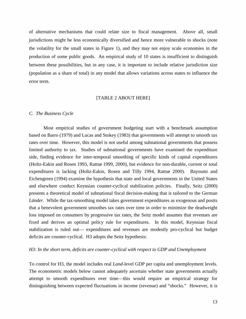
C. The Business Cycle

Most empirical studies of government budgeting start with a benchmark assumptionbased on Barro (1979) and Lucas and Stokey (1983) that governments will attempt to smooth taxrates over time. However, this model is not useful among subnational governments that possesslimited authority to tax. Studies of subnational governments have examined the expenditureside, finding evidence for inter-temporal smoothing of specific kinds of capital expenditures(Holtz-Eakin and Rosen 1993, Rattsø 1999, 2000), but evidence for non-durable, current or totalexpenditures is lacking (Holtz-Eakin, Rosen and Tilly 1994, Rattsø 2000). Bayoumi andEichengreen (1994) examine the hypothesis that state and local governments in the United Statesand elsewhere conduct Keynsian counter-cyclical stabilization policies. Finally, Seitz (2000)presents a theoretical model of subnational fiscal decision-making that is tailored to the GermanLänder. While the tax-smoothing model takes government expenditures as exogenous and positsthat a benevolent government smoothes tax rates over time in order to minimize the deadweightloss imposed on consumers by progressive tax rates, the Seitz model assumes that revenues arefixed and derives an optimal policy rule for expenditures. In this model, Keynsian fiscalstabilization is ruled out— expenditures and revenues are modestly pro-cyclical but budgetdeficits are counter-cyclical. H3 adopts the Seitz hypothesis:

H3: In the short term, deficits are counter-cyclical with respect to GDP and Unemployment

To control for H3, the model includes real Land-level GDP per capita and unemployment levels.The econometric models below cannot adequately ascertain whether state governments actuallyattempt to smooth expenditures over time—this would require an empirical strategy fordistinguishing between expected fluctuations in income (revenue) and “shocks.” However, it is

14

possible to examine whether deficits and expenditures move with or against the business cycle.H3 seems especially plausible with respect to unemployment rates, since increases are likely toplace burdens on the social spending obligations of the Länder. Bayoumi and Eichengreen (1994)use aggregate data on the entire Land sector to conclude that the Land fiscal policy is in factcounter-cyclical. By using disaggregate GDP and unemployment data and a fully specifiedmodel it is possible to make a much firmer conclusion.

D. Electoral Budget Cycle

The literature on electoral cycles is too large to review here (See Alesina 1989, Alesinaand Roubini 1992), but the basic propositions are well known. Starting with Nordhaus (1975)and Tufte (1978), political economists have suggested that opportunistic incumbent politicianshave incentives to use the tools of fiscal and monetary policy to heat up the economy prior toelections, and several scholars have attempted to assemble empirical evidence of macroeconomicfluctuations prior to elections. Most recently, a second generation of political business cyclemodels argues that large macroeconomic fluctuations before elections are not sustainable, andinstead seeks out evidence of electoral cycles on monetary and fiscal policy instruments(Cukierman and Meltzer 1986, Rogoff and Sibert 1988, Rogoff 1990).

This latter view of electoral cycles is most appropriate for fiscal policy at the Land levelin Germany. Land governments certainly cannot manipulate macroeconomic conditions duringthe run-up to Land elections, nor do they control monetary policy instruments, but they do havecontrol over spending and borrowing decisions and even though they do not set tax rates, they areresponsible for collection. Incumbent Land governments may face incentives to increasespending on highly visible public goods or particularistic projects for important constituents orreduce their tax collection efforts during elections campaigns (Wagschal 1996).

H4: Deficits are higher in fiscal years that fall during a Land election campaign period.

The campaign period is defined as the six-month period preceding any Land election. Ifthe election is held in July or later (the full six month campaign period falls in the same calendaryear as the election), the Land-year is coded as 1 for the electoral budget cycle variable. If theelection is held during the months of March through June, the year of the election receives a .5,along with the previous year. If the election is held during January or February, the deficit effect

15

would show up primarily in the previous year, so the election year receives a 0, while theprevious year receives a 1.11

E. Partisan Budget Cycle

The literature on partisan economic cycles is also voluminous. Since Douglas Hibbs(1977), political economists have argued that parties of the left and right represent the interests ofdifferent constituencies and, when in office, promulgate policies that favor them. In particular,Hibbs assumes that left-wing parties are more concerned with the problem of unemployment andright-wing parties are more concerned with inflation. This implies that partisan differencesshould show up in systematic and permanent differences in the unemployment/inflationcombination chosen by different political parties. The Länder certainly to not have the power tochoose these combinations, but a more recent literature on fiscal policy may have directapplication in the Länder. First of all, the fiscal management of left-wing governments might bemarked by greater sensitivity to unemployment. Specifically, since the Länder have littleautonomy to set tax rates but considerable borrowing and spending autonomy, left-winggovernments with a commitment to combat unemployment may have no other options duringdownturns than to increase expenditures financed by borrowing. In other words, H3 above mightbe more pronounced in Länder controlled by the left.

H5: The short-term counter-cyclicality of deficits with respect to unemployment is strengthenedby left partisanship.

Partisanship might affect not only short-term management of the business cycle, but alsolong-term expenditure and borrowing patterns. In a study of the U.S. states, Alt and Lowry(1994) argue that Democrats simply prefer higher expenditure levels than Republicans, and thatstates controlled by Democrats spend (and tax) more per capita than those controlled byRepublicans. Survey data presented by Manfred Schmidt (1992: 58) shows that SPD supportersprefer higher expenditure levels than CDU supporters. Given the lack of revenue autonomy, theonly way for left-wing governments in the Länder to live up to expectations is to rely on deficitspending (Wagschal 1996).

H6: Control by left-wing parties is associated with higher deficits

11 Another strategy is to weight each year by the number of “election campaign months” that fall within it. Thisyields very similar results to those presented below.

16

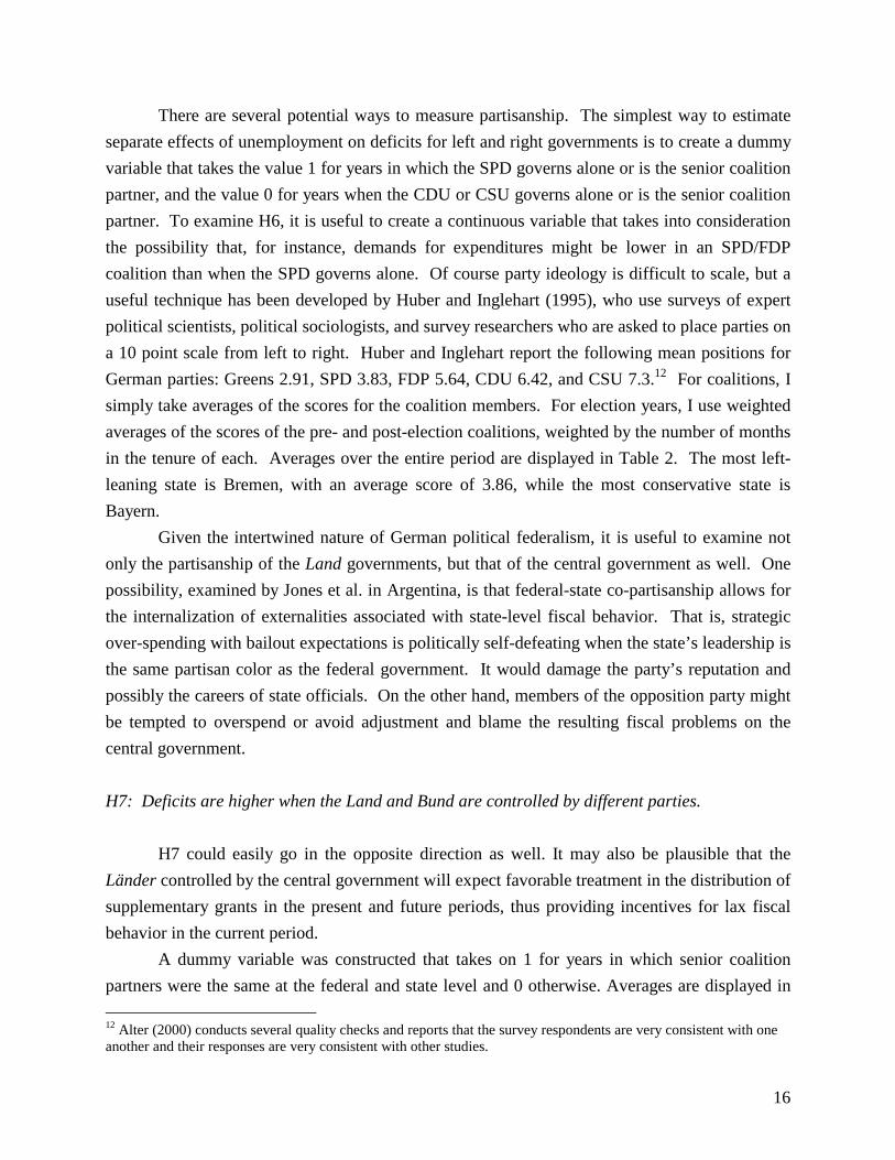
There are several potential ways to measure partisanship. The simplest way to estimateseparate effects of unemployment on deficits for left and right governments is to create a dummyvariable that takes the value 1 for years in which the SPD governs alone or is the senior coalitionpartner, and the value 0 for years when the CDU or CSU governs alone or is the senior coalitionpartner. To examine H6, it is useful to create a continuous variable that takes into considerationthe possibility that, for instance, demands for expenditures might be lower in an SPD/FDPcoalition than when the SPD governs alone. Of course party ideology is difficult to scale, but auseful technique has been developed by Huber and Inglehart (1995), who use surveys of expertpolitical scientists, political sociologists, and survey researchers who are asked to place parties ona 10 point scale from left to right. Huber and Inglehart report the following mean positions forGerman parties: Greens 2.91, SPD 3.83, FDP 5.64, CDU 6.42, and CSU 7.3.12 For coalitions, Isimply take averages of the scores for the coalition members. For election years, I use weightedaverages of the scores of the pre- and post-election coalitions, weighted by the number of monthsin the tenure of each. Averages over the entire period are displayed in Table 2. The most left-leaning state is Bremen, with an average score of 3.86, while the most conservative state isBayern.

Given the intertwined nature of German political federalism, it is useful to examine notonly the partisanship of the Land governments, but that of the central government as well. Onepossibility, examined by Jones et al. in Argentina, is that federal-state co-partisanship allows forthe internalization of externalities associated with state-level fiscal behavior. That is, strategicover-spending with bailout expectations is politically self-defeating when the state’s leadership isthe same partisan color as the federal government. It would damage the party’s reputation andpossibly the careers of state officials. On the other hand, members of the opposition party mightbe tempted to overspend or avoid adjustment and blame the resulting fiscal problems on thecentral government.

H7: Deficits are higher when the Land and Bund are controlled by different parties.

H7 could easily go in the opposite direction as well. It may also be plausible that theLänder controlled by the central government will expect favorable treatment in the distribution ofsupplementary grants in the present and future periods, thus providing incentives for lax fiscalbehavior in the current period.

A dummy variable was constructed that takes on 1 for years in which senior coalitionpartners were the same at the federal and state level and 0 otherwise. Averages are displayed in 12 Alter (2000) conducts several quality checks and reports that the survey respondents are very consistent with oneanother and their responses are very consistent with other studies.

17

Table 2, showing that Saarland’s voters are remarkably adept at bucking national trends—only10 percent of the time was the Land government controlled by the federal majority party. At theother end, the figure is around 60 percent for Baden-Wuerttemberg, Bayern, and Hessen. A morecomplex variable was also created as follows: When the federal and Land governments have noparties in common, the case receives 0 points. When the junior coalition partners are the samebut the senior partners differ, the case receives 1 point.13 When the senior coalition partners atboth levels are the same, but each has a different junior coalition partner, the case receives 2points. When either (a) the coalitions are identical or (b) the Land party governs alone while itsfederal counterpart is the senior coalition partner in Bonn, the case receives 3 points. Again,election years in which changes take place are weighted averages of the two scores.

F. Political Fragmentation

Several theories suggest that fragmented or polarized coalitions run larger deficits andaccrue higher levels of public debt. Roubini and Sachs (1989a, 1989b), Alesina and Drazen(1991), and Drazen and Grilli (1993) argue that when persistent deficits become problematic,parties in government are likely to disagree about who should bear the costs of adjustment. Inthe case of unified, single-party government, it should be relatively easy to externalize these costsonto some group that is not part of the governing party's constituency. When two or more partiesmust agree, however, either because of coalition government, or because of divided governmentbetween branches, distributional conflicts over the costs of adjustment may prevent or delay thenecessary adjustments to taxes or spending. Again, the empirical method used here does notdifferentiate between expected and unexpected shocks in order to explicitly examine adjustment,but the logic should lead to larger deficits in states with more veto players.

H8: More political fragmentation is associated with higher deficit levels.

Although the measurement of such a variable is rather complicated when comparingcountries, it is relatively straightforward in the Land context. Following Tsebelis (1995), Iassume that each coalition member is a potential veto player, so one point is assigned for eachcoalition member. A single-party government receives one point and a two-party coalitionreceives two points (there are no three party coalitions during this period). Again, whennecessary, election years are coded by using weighted averages. Perhaps a better alternativemeasurement goes beyond the number of veto players and considers their ideological spread. A 13 This was quite rare. The only scenario in which this is the case, in fact, is when the FDP is in coalition with theCDU at one level and the SPD at the other.

18

coalition with large ideological distance separating its members might find it harder to allocatecosts of adjustment. This variable takes on the value zero for one-party governments, and thedistance between the Huber-Inglehart scores for two-party coalitions. The largest ideologicalspread is, of course, a grand coalition of the CDU and SPD (2.59); the smallest is between theCDU and FDP (.78). Table 2 shows that the average ideological spread in Bayern and Schleswig-Holstein was zero. Bavaria has been controlled by the CSU alone during the entire period, andSchleswig-Holstein moved directly from the CDU alone to the SPD alone in 1988. Hessen hasbeen the most fragmented state, with three different types of coalitions during the period underanalysis.

G. Electoral Competitiveness

Alesina and Tabellini (1990) and Persson and Tabellini (2000) explore the possibility thatdebt is used strategically by politicians who expect to lose elections and seek to tie the hands oftheir successors by forcing them to take on debt payments that crowd out other forms ofexpenditure. This leads to the hypothesis that deficits are larger in extremely competitivepolitical systems where incumbents frequently have low reelection expectations. Noting thatvery little empirical support has been found for this hypothesis, Alt Lassen and Skilling (2000)propose a slightly different model that produces the opposite prediction. Their model suggeststhat in a highly competitive political system in which incumbency is shared evenly betweencompeting parties, incumbent party a is concerned that if it loses power to party b, rather thansimply being saddled with unwanted debt, b will be able to impose some of the costs ofadjustment onto the constituents of a. Thus high probability of losing office gives incumbentsincentives to seek compromise and avoid unnecessary deficits, while incumbents who do not fearremoval from office will feel free to raise debt because they expect to maintain control over theallocation of the adjustment burden.14

H9: Lower levels of political competition are associated with larger deficits.

I use an index of political competition used by Alt, Lassen, and Skilling, calculated as 1minus a Herfindahl “political concentration index”: 1-Σ αi

2 where αi is the proportion of time inoffice (as senior coalition partner) for party i, and Σ αi

2 = 1. The competition index moves from0 to 1 as competition increases. Table 2 shows that when a state has been completely dominatedby one party (e.g. Bayern), the index is zero. The most competitive state is Schleswig-Holstein at 14 Their model also includes an additional fiscal discipline mechanism associated with electoral competition. Party bwill be able to open the books and reveal any inefficient behavior undertaken by a.

19

.43 (.5 would indicate incumbency shared evenly between the CDU and the SPD). This index isuseful for cross-sectional analysis, but it does not vary over time. For time-series cross-sectionanalysis, it is difficult to come up with a proxy of “incumbent’s perceived reelection probability.”The most reasonable proxy is the incumbent senior coalition partner’s vote share in the mostrecent election.

V. Empirical Approach

The data set consists of observations for each of the “old” German Länder for each yearbetween 1974 and 1995.15 A very short time series and vastly different budgeting circumstancesmitigate against including the new Länder. Likewise, the special status of Berlin both before andafter unification requires that it be excluded. Additionally, the years 1994 and 1995 are droppedfor Bremen and Saarland because massive bailouts received in those years caused grants toballoon, and budgets were ‘artificially’ balanced by federal intervention. In addition to the Landaverages presented in Table 2, Table 3 presents descriptive statistics.


Several potential econometric strategies present themselves. Hypotheses related

exclusively to fiscal adjustment are best tested by examining expenditure responses to expected

and unexpected changes in income or revenue. However, the focus of this paper is on

determinates of deficits, and the goal is to provide the most complete specification possible.

Some of the hypotheses presented above are primarily about cross-Land differences, while others

require analysis of changes over time within Länder —some short-term and some long-term.

Consider the role of partisanship. H5 requires time-series cross-section analysis of short-term

changes in unemployment, estimating separate effects for left- and right-controlled governments.

Such a model should focus on changes and include fixed Land effects. However, H6 (the

independent effect of ideology on deficits) cannot very well be tested with a first differenced

model including fixed effects because the partisan compositions of the Länder are very stable

15 Data on government composition, election timing, and vote shares were taken from the American Institute forContemporary German Studies (http://www.jhu.edu/~aicgsdoc/wahlen). Fiscal, unemployment, and population datawere downloaded from the Statistisches Bundesamt (http://www.statistik-bund.de). GDP data were kindly providedby the statistical office of Baden-Wuerttemberg. These data were also used to calculate Land-level deflators used toadjust all fiscal data for inflation.

20

over time. Moreover, the argument behind H1 (transfer dependence) requires a model that

differentiates between short-term and long-term effects.

To address these concerns, the empirical analysis proceeds in three stages. The first and

most reliable group of time-series cross-section models uses the error correction set-up to

differentiate between short- and long-term effects of key variables. These models focus on

changes and include Land dummies to remove cross-section effects. Next, in order to allow for

some cross-sectional effects, a model is estimated using levels and dropping the fixed effects.

Finally, in spite of the low degrees of freedom (only 10 Länder), it is instructive to estimate a

simple between-effects model on cross-section averages to illuminate the effects of persistent

cross-state differences.

Given that the data set includes 10 cross-section units and 21 years and includes lags and

fixed effects, one must be concerned about obtaining biased estimates with any estimation

technique. Monte Carlo analysis by Judson and Owen (1999) suggests that the 1-stage GMM

estimator slightly out-performs the LSDV estimator for such a data set. Thus the results below

are estimated using the GMM estimator derived by Arellano and Bond (1991), but in fact very

similar results can be obtained with OLS or LSDV using panel-corrected standard errors. The

Arellano-Bond technique relies on the use of first-differences and instrumental variable

estimation, where the instruments are the lagged explanatory variables (in differences) and the

dependent variable in level lagged twice.16 As recommended by Arellano and Bond, (1991) one-

step robust results are presented and used for inference on coefficients. The error correction

version of the model looks like this:

∆ Surplus (t) = β0 + β1Surplus (t-1) + β2∆Surplus (t-1) + β3∆Grants (t) + β4Grants (t-1) + β5∆GDP (t) + β6GDP

(t-1) + β7∆Unemployment x Right(t) + β8∆Unemployment x Left(t) + β9Unemployment x Right(t-1) +

β10Unemployment x Left(t-1) + β11Ideology(t) + β12Election Year(t) + β13Partisan Similarity(t) +

β14Fragmentation(t) + β15Most Recent Vote Share(t) + Land and Year Dummies + ε

The dependent variable is the change in real surplus per capita.17 The lagged change and

lagged level of the dependent variable are included. The use of both levels and changes on the

economic variables allows for a straightforward interpretation of their effects. The coefficient on

16 This approach was first suggested by Anderson and Hsiao (1981) and developed further by Arellano and Bond (1991). For anoverview, see Baltagi (1995), chapter 8.17 Surpluses are positive numbers and deficits are negative.

21

the lagged level of real grants per capita measures the long-term or permanent effect on the

surplus (H1), while the coefficient for the first difference measures short-term or transitory

effects. Similarly, the coefficients for the lagged levels of GDP and unemployment estimate the

long-term effects of economic change, while the coefficient for the change variable allows one to

examine short-term responses to the business cycle (H2). In accordance with H5, separate

unemployment effects are estimated for left- and right-run governments. The election year

dummy is included (H4), along with the continuous ideology variable (H6), the vertical partisan

similarity dummy (H7), the continuous political fragmentation variable (H8), and the vote share

of the senior coalition member in the most recent election (H9). The model also includes a full

set of Land dummies, and in order to control for the impact of events like the oil crisis in the

early 1970s and unification in the early 90s, a full set of year dummies is included as well.


The results of this model are presented in Table 4. In addition to the surplus model,

Table 4 also reports the results of identical models that use real expenditures per capita and real

revenues per capita as dependent variables. For some of the hypotheses, it is helpful to examine

whether variables that effect fiscal balance are working through the expenditure side or the

revenue side or both. Each of these models performs well. For each model, a Wald test of the

null that all of the coefficients except the constant are zero is soundly rejected, and an Arellano-

Bond test finds no evidence of first- or second- order auto-correlation in the differenced

residuals. The results presented in Table 4 should be quite trustworthy. Similar results have

been obtained using other estimation techniques, and experiments with dropping states reveal

that the results are not driven by outliers (e.g. Bremen or Saarland).


The results presented in Table 5 must be approached with more caution, but they provide

valuable information. These models use the OLS estimator (with panel-corrected standard errors

and a lagged dependent variable) using levels at year t and dropping the Land dummies in order

to allow cross-state variation to affect the results. This allows for a better examination of factors

22

like ideology that change little over time within states, but the results are more sensitive to the

inclusion and exclusion of cases, and it is difficult to distinguish between short- and long-term

relationships. Since H1 only deals with the long-term effects of grants, these models use a 5-year

moving average rather than yearly levels of the grant variable.


Finally, Table 6 presents the results of the most blunt models—OLS regressions on cross-

section averages. All of the variables are the same except the political competition index, which

replaces the vote share of the governing party as the indicator of electoral competitiveness. Of

course one should not expect significant results when 8 variables are included and n=10, but

several variables do approach statistical significance in the full model. Table 6 presents the

results of models that drop the one variable (political fragmentation) that does not come close to

significance in the full model. The models explain over 99 percent of the cross-state variation in

surplus, revenue, and expenditure, and several coefficients attain significance at the 5 percent

level.

VI. Results

A. Equalization and Grants

The results presented in Tables 4 through 6 tell an interesting story about

intergovernmental grants in Germany. First of all, short-term increases in grants have a large

positive effect on fiscal balance (the first column in Table 4). Not surprisingly, other things

equal, increases in grants have large positive effects on revenues (the third column), but it is

quite interesting that they have no discernable effect on expenditures in the short term (the

second column). This may suggest that Land decision-makers are attempting to smooth out short-

term fluctuations in grants.

However, upon examination of the coefficients for lagged grant levels, there appears to be

strong support for H1. Controlling for developments in GDP and unemployment, a long-term

increase of 100 DM per capita in intergovernmental grants is associated with a decrease of 13

DM per capita in fiscal balance. The revenue and expenditure equations show that an increase of

23

100 DM in grants is associated with only 30 DM in increased total revenue, but an increase of 86

DM in expenditures. Thus there appears to be a long-term flypaper effect—increases in grants

stimulate increased expenditures and larger deficits.18 Note that these results are not affected by

cross-state differences, but rather exclusively by developments within states over time. In Table

5, which does allow for cross-sectional variation, the coefficient for the moving average of real

grants per capita is even larger and significant at the five percent level, and again, the coefficient

in the expenditure equation is over twice as large as that in the revenue equation. Finally, Table

6 and the scatter-plot presented in Figure 4 tell a similar story—other things equal, more transfer-

dependent Länder run larger deficits.


One might suspect that grant levels should be treated as endogenous. First of all, it seems

plausible that if grants are used as a kind of gap-filling, a deficit in year t might “cause” higher

grants in year t+1. However, Granger causality tests (not reported) showed that no matter what

lag structure is used, there is no evidence that deficits “cause” grants. Furthermore, one might

suspect that a two-equation system would be preferable if increasing grants are in fact driven by

changes in unemployment, GDP, or partisan composition. However, these variables perform

surprisingly poorly in regressions on grants per capita.

B. Jurisdiction Size

Since the models in Table 4 control for fixed effects, the size variable is only included in the

models in Table 5 and 6. Table 5 suggests that smaller states run larger deficits, though the

coefficient is only significant at the ten percent level. The coefficient in the between-group

effects model presented in Table 6 does not quite obtain significance, but does so in a variety of

pared-down specifications. The relationship is demonstrated in Figure 5. However, it is not

possible to draw any conclusions about causality—explanations based on scale economies,

volatility, and moral hazard are all plausible.

18 A concern with this model is that grants may be a mere reflection of fluctuations in unemployment and GDP ifthey are redistributive by design. However, unemployment and GDP per capita perform rather poorly in regressions

24


C. Business Cycle

It is possible to reject rather firmly the notion that the Länder conduct counter-cyclical

fiscal policy. In fact, the evidence suggests procylicality. The “GDP change” line in Table 4

shows that revenues and expenditures move with the business cycle—revenues more so than

expenditures—but fluctuations in GDP have no discernable effect on deficits.19 The coefficients

for revenue and expenditures are virtually identical to those in a recent study by Seitz (2000) that

uses a different estimation technique.20 The “change in unemployment” coefficients (broken

down into separate coefficients for CDU-led and SPD-led governments) are positive for the

surplus, again indicating pro-cyclicality. As unemployment rates go up, the equalization system

does apparently respond with extra revenue (the coefficients in the right hand column are positive

and significant), but expenditures go down and the surplus actually goes up. Together with Seitz

(2000), these results confirm that there is nothing like Keynsian counter-cyclical fiscal

management going on in the German federal system.

D. Electoral Budget Cycle

The analysis finds strong support for the electoral budget cycle hypothesis. Table 4

suggests that state governments spend an extra 46 DM per capita during election years, and the

deficit expands by 57 DM per capita. The revenue result is quite interesting as well. Even though

the states have very limited authority over tax rates, their discretion in collection appears to allow

them to reduce revenue collection by around 21 DM per capita during election years. Note that

the specifications in Table 4 include dummies for each year, which tends to suppress the

significance of the election year dummy. When the year dummies are excluded, the election year

on grants per capita (not reported). The correlation between grants and GDP is .11, and between grants andunemployment is .5.19 The coefficients for lagged GDP demonstrate that in the long run as states get wealthier, they spend and borrowmore.20 The only difference is that Seitz finds evidence in favor of modestly counter-cyclical deficits.

25

dummy is significant at the one percent level in each model, and the coefficients are substantially

higher.

E. Partisan Budget Cycle

In both the short- and the long-term, Table 4 suggests that CDU-led and SPD-led Länder

have very similar responses to changes in unemployment—the positive (pro-cyclical) coefficients

are virtually identical. Separate effects for GDP on fiscal outcomes in left- and right-run Länder

(not reported) also did not yield significant differences between the two types of government.

These findings are quite similar to those reported in Seitz (2000). Thus considerable doubt is cast

upon H5, and the ideology variable (H6), though positive as predicted, is not statistically

significant. However, given the stability of partisan composition in most of the Länder,21 it is

necessary to introduce cross-section variation to test H6. Table 5 demonstrates that more

conservative Länder spend less and run smaller deficits. Table 6 and Figure 6 show that the

relationship is indeed driven by persistent cross-Land variation.


Turning to H7, no support is found for the proposition that federal-state co-partisanship

affects fiscal outcomes in the fixed-effects models. In the model without fixed effects, the

coefficient is the opposite of that predicted by H7. That is, expenditures were higher and deficits

larger in states controlled by the party in power in Bonn. It should be noted, however, that this

finding is quite vulnerable to alternative specifications, and when the alternative three-point

variable is used, the coefficient is not statistically significant. It also does not achieve

significance in the simple cross-section model.

F. Political Fragmentation

No support is found for the common wisdom that political fragmentation leads to budget

deficits (H8). In fact, in the model with fixed effects, the coefficient is positive and significant,

suggesting that greater ideological spread between coalition members is associated with smaller

deficits. Again, though, the significance of this coefficient is sensitive to the estimation

26

technique employed and the variables included, and the result should be approached with

caution.

G. Political Competition

The vote share of the senior coalition partner in the most recent election—an (admittedly

imperfect) proxy for reelection expectations—does not perform well in time-series cross-section

models, but the political competition index does achieve significance at the ten percent level in

the cross-section model. However, Figure 7 casts some doubt on the relationship. On the left

hand side, a number of states have been dominated by the SPD or CDU/CSU (the index =0), with

widely varying fiscal outcomes ranging from Bayern’s balanced budgets to Bremen’s massive

deficits, though it is also true that none of the states with high levels of political competition run

large deficits.

All in all, it is difficult to make firm assessments of H8 and H9. They both might capture

different aspects of the competitiveness of Land-level politics. The fragmentation index assesses

whether the governing party (CDU or SPD) must share power and with whom, while the

competition index measures the long-term alteration in governing parties. Although the results

are rather weak, if anything they suggest that dominant single-party governments—with the

exception of CDU/CSU-dominated Baden-Wuerttemberg and Bavaria—are likely to run larger

deficits. This finding is consistent with results from a study of the Argentine states (Remmer and

Wibbels 2000).

VII. Implications and Conclusions

With their similar institutions and cultures, the German Länder present an excellent

opportunity to test a variety of general theories about politics and fiscal management that have

previously been examined only with cross-country data. Perhaps more importantly, this paper

also examines some propositions that are unique to subnational units that have expenditure and

borrowing authority but little autonomy on the revenue side—the basic situation of most state

and local governments around the world. Table 7 provides an overview of the findings.

21 In the Western Länder the best predictor of partisanship is still the Catholic-Protestant divide.

27


As in cross-national studies, the Länder appear to spend and borrow more during election years.

Although no support is found for partisan differences in the management of the business cycle,

left-wing governments do spend more and run larger deficits than right-wing governments in the

long term. The paper also suggests a weak yet potentially intriguing relationship between

political competition, partisan fragmentation, and deficits that deserves further analysis.

Both the revenues received by the Länder and their expenditures are clearly pro-cyclical.

Since they have little authority on the revenue side, and in fact many of their expenditures

involve long-term contracts and the administration of federal policy, they apparently do not have

much room to respond to shocks in unemployment and growth with countercyclical expenditures.

Thus the lack of partisan differences in short-term fiscal management should not be surprising.

More broadly, since most subnational governments around the world face constraints that are

more similar to the German Länder than those of the U.S. states, these findings cast doubt on the

U.S.-based proposition of Bayoumi and Eichengreen (1994) that subnational governments around

the world conduct significant counter-cyclical stabilization policy. The likelihood that

subnational government expenditures will be pro-cyclical should be an extremely important

consideration in the literature on the design of decentralized expenditure programs, especially in

Latin America and other developing countries.

The most striking findings presented in this paper have to do with the incentives created

by the German system of intergovernmental transfers. The equalization system provides limited

insurance against revenue shocks—it does not allow state revenues to fall far below the national

average. In doing so, it actually provides that the “last” in terms of fiscal capacity per capita are

actually “first” after equalization. But it does not provide insurance to compensate for income or

unemployment shocks (Von Hagen and Hepp 2000), and by no means does it ensure the Länder

that expenditures can maintain a constant growth trajectory. In other words, Länder are not

relieved of the obligation to undertake politically painful expenditure adjustments. However, a

constantly increasing flow of discretionary supplementary grants could easily create this

impression. This paper has argued that these grants—coupled with the constitutional obligation

to maintain equivalent living conditions—provide politicians with rational beliefs that current

deficits can be shifted onto residents of other jurisdictions in the future through increased

28

transfers. Even if unsure whether these bailouts will be provided and precisely what form they

will take, politicians in the most transfer-dependent states have few reasons to fear the wrath of

voters and creditors if their debt servicing burden increases.

The findings in this paper are quite consistent with this argument. In the long run within

and across states, increasing dependence on grants is associated with higher spending and larger

deficits. Since the models control for a wide range of other plausible explanations for fiscal

outcomes including state-level income and unemployment, it is reasonable to assume that these

coefficients reflect the independent effect of transfers on fiscal behavior. Future studies might

examine H1 more carefully by examining expenditure responses to expected fluctuations and

“shocks” in revenues and income to see if there are differences in fiscal management between the

“paying” and “receiving” Länder in the equalization process. In particular, H1 suggests that the

“receiving” Länder are less responsive to negative shocks.

By no means does this paper suggest that the more transfer-dependent states are engaged

in a self-conscious and conspicuous strategy of running unsustainable deficits and demanding

bailouts. Prior to recent court decisions, no one knew how the federal government and courts

would deal with bailout requests; Bremen and Saarland were charting new territory. Now that

the precedent has been set, it does appear that any future bailouts will be associated with

considerable loss of discretion over expenditures and as a result, political embarrassment. In the

wake of high profile bailouts, states are not necessarily inclined to “play the Bremen strategy.” If

anything, they might have increased their fear of losing control over expenditures.22 Only time

will tell if the strings attached to recent bailouts imply that a new game is now being played.

Thus it is not correct to conclude that the “receiving” Länder—these are now predominantly the

new eastern Länder—can be expected to throw fiscal caution to the wind in the future. Though it

is alarming to note that Berlin seems to be going the way of Berlin and Saarland, refusing to take

efforts to reduce its staggering debt burden while intimating that the ultimate resolution will

require federal intervention.

The gap between the transfer-paying and transfer-receiving Länder has grown into an

important political division as wealthy states like Baden-Württemberg and Bavaria have become

increasingly vocal in demanding reforms to the equalization system. In June of 2001, the Bund

and Länder agreed to a new equalization law, to take effect in 2005. The basic structure of the

22 Thanks to Helmut Seitz for pointing this out.

29

old three-stage system remains unchanged, but the wealthy states agreed to the new system

because it allows them to keep a larger share of the taxes they collect.23 But the agreement will

not reduce the receipts of the relatively poor Länder. This apparent “win-win” scenario was

possible because the central government agreed to make up the difference by committing billions

of additional DM to the system. In other words, the central government will be replacing some

of the horizontal redistribution between the Länder with direct, vertical redistribution from the

Bund to the Länder, and transfer-dependence among the poorest Länder will only grow. Though

many details of the new system remain unresolved—including the possibility of new nation-wide

debt restrictions imposed on the Länder—this does not bode well for fiscal performance among

the recipient states if current trends continue.

23 There will be a ceiling on the amount that a Land must contribute to equalization—no more than 72.5 percent ofthe amount of its tax income that is above the national average. Länder will also be able to keep 12.5 percent of theamount of any yearly increase in tax receipts that surpasses the national average increase.

30

References

Alesina, Alberto. 1989. "The End of Large Public Debts," in Giavazzi and Spaventa, eds., High Public Debt: THeItalian Experience, Cambridge: Cambridge University Press.

Alesina, Alberto and Tamim Bayoumi. 1996. "The Costs and Bendefits of Fiscal Rules: Evidence from U.S.States," Cambridge, MA: NBER Working Paper no. 6914.

Alesina, Alberto and R. Perotti, "The Political Economy of Budget Deficits," Cambridge, MA: NBER WorkingPaper no. 4637.

Alesina, Alberto and Noriel Roubini. 1992. "Positive and Normative Theories of Public Debt and Inflation inHistorical Perspective," European Economic Review, 36:2, 337-44

Alesina, Alrberto and Guido Tabellini. 1990. "A Positive Theory of Budget Deficits and Government Debt,"Review of Economic Studies 57, 403-14.

Alt, James and Robert Lowry. 1994. "Divided Government, Fiscal Institutions, and Budget Deficits: Evidencefrom the States," Americal Political Science Review 88:4 (December), 811-828.

Alt, James, David Dreyer Lassen and David Skilling. 2001. “Fiscal Transparency and Fiscal Policy Outcomes inOECD Countries.” Paper presented at the 2001 Annual Meeting of the Midwest Political Science Association,Chicago, IL.

Alter, Alison. 2000. “Minimizing the Risks of Delegation: Multiple Referral in the German Budesrat,” paperpresented at the 2000 Annual Meeting of the American Political Science Association.

Anderson, T.W. and Cheng Hsaio. 1981. “Estimation of Dynamic Models with Error Components.” Journal of theAmerican Statistical Association 76 (2): 598-606.

Arellano,Manuel and Stephen Bond. 1991. “Some Tests of Specification for Panel Data: Monte Carlo Evidenceand an Application to Employment Equations,” Review of Economic Studies 58, p. 277-97.

Baltagi, Badi. 1995. Economic Analysis of Panel Data. West Sussex, England: Wiley.

Barro, Robert. 1979. "On the Determination of Public Debt," Journal of Political Economy 87, 940-7.

Bayoumi, Tamim and Barry Eichengreen. 1994. “Restraining Yourself: Fiscal Rules and Stabilization,” Centre forEconomic Policy Research, Discussion Paper No. 1029.

Bevilaqua, Afonso. 1999. “State Government Bailouts in Brazil,” unpublished paper, Inter-American DevelopmentBank, Washington, D.C.

Bohn, Henning and Robert Inman. 1996. "Balanced Budget Rules and Public Deficits: Evidence from the U.S.States," Carnegie-Rochester Conference Series on Public Policy 45: 13-76.

Cukierman, A. and A. Meltzer. 1989. "A Political Theory of Government Debt and Deficits in a Neo-RicardianFramework," American Economic Review 79, 713-33.

Deutsche Bundesbank. 1997. "Die Entwicklung der Staatsverschuldung seit der deutschen Vereinigung," MonthlyReport, No. 3 (March). Frankfurt: Deutsche Bundesbank.

Dillinger, William and Steven Webb. 1999. “Fiscal Management in Federal Democracies: Argentina and Brazil.”Policy Research Working Paper Number 2121. Washington, D.C: World Bank.

31

Drazen, A. and V. Grilli. 1993. "The Benefit of Crises for Economic Reform," American Economic Review 83:2,588-608.

Eichengreen, Barry and Jürgen von Hagen. 1996. "Fiscal Restrictions and Monetary Union: Rationales,Repercussions, Reforms." Empirica 23: 3-23.

Fornasari, Francesca, Steve Webb, and Heng-Fu Zou. 1998. "Decentralized Spending and Central GovernmentDeficits: International Evidence." Washington, D.C.: World Bank.

Franzese, Robert. 1996. "The Political Economy of Public Debt: An Empirical Examination of the OECD Post-War Experience," paper presented at the annual meeting of the Midwest Political Science Association, April9, 1996.

Gramlich, Edward. 1991. "The 1991 State and Local Fiscal Crisis," Brookings Papers on Economic Activity 2:1991.

Hibbs, Douglas. 1977. "Political Parties and Macroeconomic Policy," American Political Science Review 71, 1467-87.

Holtz-Eakin, Douglas and Harvey Rosen. 1993. “Municipal Construction Spending: An Empirical Examiniation,”Economics and Politics 5, 1: p. 61-84.

Holtz-Eakin, Douglas, Harvey Rosen and Schuyler Tilly. 1994. “Intertemporal Analysis of State and LocalGovernment Spending: Theory and Tests,” Journal of Urban Economics 35, p. 159-174.

Huber, John and Ronald Inglehart. 1995. “Expert Interpretations of Party Space and Party Locations in 42Societies.” Party Politics 1, 1: 73-111.

Inman, Robert. 1997. Do Balanced Budget Rules Work? U.S. Experience and Possible Lessons for the EMU,NBER Reprint No. 2173.

Jones, Mark, Pablo Sanguinetti and Mariano Tommasi. 2000. Politics, Institutions, and Fiscal Performance in aFederal System: An Analysis of the Argentine Provinces. Journal of Development Economics 61, 2: 305-33.

Judson, Ruth and Ann Owen. 1999. “Estimating dynamic panel data models: a guide for macroeconomists.”Economic Letters 65, 9-15.

Lohmann, Susanne, David Brady and Douglas Rivers. 1997. "Party Identification, Retrospective Voting, andModerating Elections in a Federal System: West Germany, 1961-1989," Comparative Political Studies 30:4(August), 420-449.

Lowry, Robert, James Alt and Karen Ferree. 1998. "Fiscal Policy Outcomes and Electoral Accountability inAmerican States," American Political Science Review 92, 4: 759-74.

Lucas, R. and N. Stokey. 1983. "Optimal Fiscal and Monetary Policy in an Economy without Capital," Journal ofMonetary Economics 12:1, 55-94.

McKinnon, Ronald. 1997. "Monetary Regimes, Government Borrowing Constraints, and Market-PreservingFederalism: Implications for EMU," in Thomas Courchene, ed., The Nation State in a Global/Information Era:Policy Challenges. Kingston, Ont: John Deutsch Institute.

Nordhaus, William. 1975. "The Political Business Cycle," Review of Economic Studies 42, 169-90.

Persson, Torsten and Guido Tabellini. 2000. Political Economics: Explaining Economic Policy. Cambridge, MA:MIT Press.

32

Poterba, James. 1994. "State Responses to Fiscal Crises: "Natural Experiments" for Studying the Effects ofBudgetary Institutions," Journal of Political Economy.

_____. 1996. "State Responses to Fiscal Crises: The Effects of Budgetary Institutions and Politics," Journalof Political Economy 102:4, 799-821.

Rattsø, Jørn. 1999. “Aggregate Local Public Sector Investment and Shocks: Norway 1946-1999.” AppliedEconomics 31, p. 577-584.

_____. 2000. “Fiscal Adjustment with Vertical Fiscal Imbalance: Empirical Evaluation of Administrative FiscalFederalism in Norway,” unpublished paper, Norwegian University of Science and Technology, Trondheim, Norway.

Remmer, Karen and Erik Wibbels. 2000. “The Subnational Politics of Economic Adjustment: Provincial Politics andFiscal Performance in Argentina.” Comparative Political Studies 33, 4: 419-451.

Renzsch, Wolfgang. 1991. Finanzverfassung und Finanzausgleich. Bonn: Dietz.

Rodden, Jonathan. 2001. “The Dilemma of Fiscal Federalism: Grants and Fiscal Performance around the World.”Typescript, MIT.

_____. 2001. “Soft Budget Constraints and German Federalism.” In Rodden, Jonathan, Gunnar Eskeland andJennie Litvack, eds. 2001. Decentralization and the Challenge of Hard Budget Constraints. Forthcoming,Cambridge: MIT Press.

Rodden, Jonathan, Gunnar Eskeland and Jennie Litvack, eds. 2001. Decentralization and the Challenge of HardBudget Constraints. Forthcoming, Cambridge: MIT Press.

Rogoff, Kenneth. 1990. "Equilibrium Political Budget Cycles," American Economic Review 80:1, 21-36.

Rogoff, Kenneth and Anne Sibert. 1988. "Equilibrium Political Business Cycles," Review of Economic Studies 55,1-16.

Roubini, Noriel and Jeffrey Sachs. 1989a. "Political and Economic Determinants of Budget Deficits in theIndustrial Democracies," European Economic Review 33:2, 903-33.

_____. 1989b. "Government Spending and Budget Deficits in the Industrialized Countries," Economic Policy 8,99-132.

Sachverst←ndigenrat. 1997. Wachstum, Beschäftigung, Währungsunion- Orientierung für die Zukunft:Jahresgutachten 1997/1998. Stuttgart: Metzler-Poeschel.

Scharpf, Fritz. 1994. Optionen des Föderalismus in Deutschland und Europa. Frankfurt: Campus Verlag.

Scharpf, Fritz, Bernd Reissert and Fritz Schnabel . 1976. Politikverflechtung: Theorie und Empirie deskooperativen Föderalismus in der Bundesrepublik. Kronberg: Scriptor.

Schmidt, Manfred. 1992. Regieren in der Bundesrepublik Deutschland. Opladen: Leske und Budrich.

Seitz, Helmut. 1998. “Subnational Government Bailouts in Germany,” unpublished paper, Center for EuropeanIntegration Studies, Bonn.

_____. 2000. “Fiscal Policy, Deficits and Politics of Subnational Governments: the Case of the German Laender,”Public Choice 102: 183-218.

Spahn, Paul Bernd and Wolfgang Föttinger. 1997. "Germany," in Teresa Ter-Minassian, ed., Fiscal Federalism inTheroy and Practice. Washington, D.C.: International Monetary Fund.

33

Tanzi, Vito. 1995. "Fiscal Federalism and Decentraliztaion: A Review of Some Efficiency and MacroeconomicAspects," in World Bank Annual Conference on Development Economics. Washington, D.C.: World Bank.

Triesman, Daniel. 2000. "Decentralization and Inflation: Commitment, Collective Action, or Continuity?” AmericanPolitical Science Review 94: 837-858.

Tsebelis, George. 1995. "Decision-Making in Political Systems: Veto Players in Presidentialism, Parliamentarism,Multicameralism and Multipartism," British Journal of Political Science 25:3, 289-326.

Tufte, Edward. 1978. Political Control of the Economy. Princeton: Princeton University Press.

Von Hagen, Jürgen and Barry Eichengreen. 1996. "Federalism, Fiscal Restraints, and European Monetary Union,"American Economic Review 86:2, May.

Von Hagen, Jürgen, Massimo Bordignon, Matz Dahlberg, Bhahan Grewal, Per Petterson and Helmut Seitz. 2000.“Subnational Government Bailouts in OECD Countries: Four Case Studies.” Inter-American Development BankWorking Paper R-399.

Von Hagen, Jürgen and Ralf Hepp. 2000. “Regional Risksharing and Redistribution in the German Federation.”Unpublished working paper, Center for European Integration Research, Bonn.

Wagschal, Uwe. 1996. "Der Einfluss von Parteien und Wahlen auf die Staatsverschuldung," SchweizerischeZeitschrift für Politische Wissenschaft 2:4 (winter).

Winer, Stanley. 1983. "Some Evidence on the Effect of the Separation of Spending and Taxing Decisions," Journalof Political Economy 91:1.

Wildasin, David. 1997. “Externalities and Bailouts: Hard and Soft Budget Constraints in Intergovernmental FiscalRelations.” Typescript. Vanderbilt University.

34

Surplus/Revenue (1992-1995 Ave.)

Debt/Capita (as of 31 Dec. 1996)

"Old" Länder

Baden Wuerttemberg -0.04 6539Bayern -0.01 4857Bremen* -0.14 24545Hamburg -0.12 16387Hessen -0.07 9347Niedersachsen -0.12 9974Nordrhein-Westfallen -0.06 10183Rheinland Pfalz -0.07Saarland* -0.17 15448Schleswig-Holstein -0.10 11395

New" Länder

Brandenburg -0.27 9995Mecklenburg-Vorpommern -0.17 7912Sachsen -0.12 6149Sachsen-Anhalt -0.21 9641Thueringen -0.18 9078

Table 1: Deficits and Debt in the German Länder

Sources: Federal Statistics Office, Sachverständigenrat (1997), and author's calculations.* Bremen and Saarland averages exclude 1994 and 1995, when balanced budgets resulted from federal bailouts.

35

Figure 1: Real Surplus per Capita by Land, 1974-1995

-250

-200

-150

-100

-50

0

50

1970 1975 1980 1985 1990 1995 2000

Rea

l DM

per

cap

ita

Bremen

Hamburg

Saarland

Schleswig-HolsteinNiedersachsen

HessenRheinland-PfalzBWNRW

Bayern

36

Figure 3: Real Grants per Capita by Land, 1974-1995

0

50

100

150

200

250

1970 1975 1980 1985 1990 1995 2000

Rea

l DM

per

cap

ita

Bremen

Saarland

Rheinland-Pfalz

BWNiedersachsenHamburg

Schleswig-HolsteinBayernHessenNRW

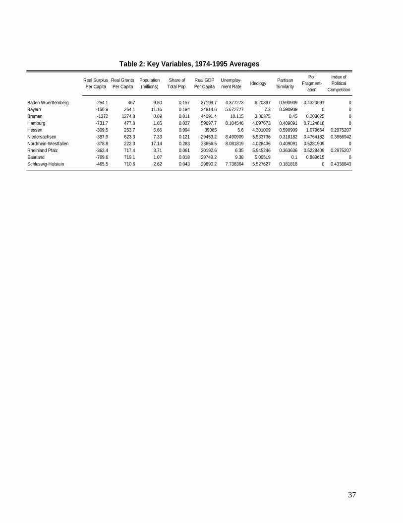
37

Real Surplus Per Capita

Real Grants Per Capita

Population (millions)

Share of Total Pop.

Real GDP Per Capita

Unemploy-ment Rate Ideology Partisan

Similarity

Pol. Fragment-

ation

Index of Political

Competition

Baden Wuerttemberg -254.1 467 9.50 0.157 37198.7 4.377273 6.20397 0.590909 0.4320591 0Bayern -150.9 264.1 11.16 0.184 34814.6 5.672727 7.3 0.590909 0 0Bremen -1372 1274.8 0.69 0.011 44091.4 10.115 3.86375 0.45 0.203625 0Hamburg -731.7 477.8 1.65 0.027 59697.7 8.104546 4.097673 0.409091 0.7124818 0Hessen -309.5 253.7 5.66 0.094 39065 5.6 4.301009 0.590909 1.079664 0.2975207Niedersachsen -387.9 623.3 7.33 0.121 29453.2 8.490909 5.533736 0.318182 0.4764182 0.3966942Nordrhein-Westfallen -378.8 222.3 17.14 0.283 33856.5 8.081819 4.028436 0.409091 0.5281909 0Rheinland Pfalz -362.4 717.4 3.71 0.061 30192.6 6.35 5.945246 0.363636 0.5228409 0.2975207Saarland -769.6 719.1 1.07 0.018 29749.2 9.38 5.09519 0.1 0.889615 0Schleswig-Holstein -465.5 710.6 2.62 0.043 29890.2 7.736364 5.527627 0.181818 0 0.4338843

Table 2: Key Variables, 1974-1995 Averages

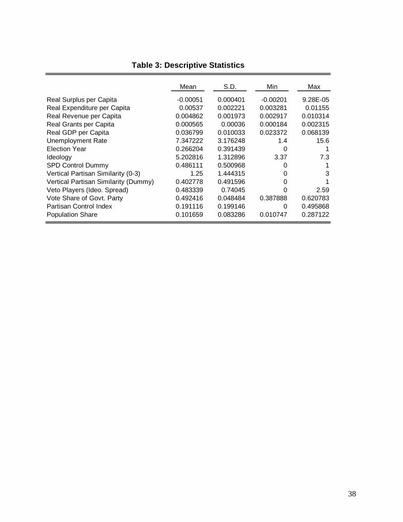
38

Mean S.D. Min Max

Real Surplus per Capita -0.00051 0.000401 -0.00201 9.28E-05Real Expenditure per Capita 0.00537 0.002221 0.003281 0.01155Real Revenue per Capita 0.004862 0.001973 0.002917 0.010314Real Grants per Capita 0.000565 0.00036 0.000184 0.002315Real GDP per Capita 0.036799 0.010033 0.023372 0.068139Unemployment Rate 7.347222 3.176248 1.4 15.6Election Year 0.266204 0.391439 0 1Ideology 5.202816 1.312896 3.37 7.3SPD Control Dummy 0.486111 0.500968 0 1Vertical Partisan Similarity (0-3) 1.25 1.444315 0 3Vertical Partisan Similarity (Dummy) 0.402778 0.491596 0 1Veto Players (Ideo. Spread) 0.483339 0.74045 0 2.59Vote Share of Govt. Party 0.492416 0.048484 0.387888 0.620783Partisan Control Index 0.191116 0.199146 0 0.495868Population Share 0.101659 0.083286 0.010747 0.287122

Table 3: Descriptive Statistics

39

Dependent Variable:

Dependent Variablet-1 -0.534 *** -0.566 *** -0.251 **(0.078) (0.123) (0.104)

∆ Dependent Variablet-1 -0.169 *** -0.094 0.094(0.042) (0.108) (0.171)

∆ Grants 0.721 *** 0.024 0.645 ***(0.116) (0.071) (0.152)

Grantst-1 -0.138 *** 0.858 *** 0.307 **(0.040) (0.166) (0.145)

∆ GDP 0.011 0.047 *** 0.093 ***(0.015) (0.018) (0.017)

GDPt-1 -0.026 ** 0.036 ** -0.0002(0.012) (0.015) (0.004)

∆ Unemployment, Right Govt. 61.5 ** -47.17 67.31 **(28.7) (40.6) (26.3)

∆ Unemployment, Left Govt. 54.7 -34.38 57.82 ***(35.3) (45.6) (22.2)

Unemploymentt-1, Right Govt. 2.9 2.47 9.9(14.6) (11.6) (6.9)

Unemploymentt-1, Left Govt. 8.5 7.12 13.14 *(14.1) (10.7) (7.1)

Ideology 28.6 9.76 5.54(25.0) (16.5) (13.7)

Election Year -57.1 ** 45.72 * -21.18 *(27.0) (27.9) (13.3)

Vertical Partisan Similarity -47.9 33.97 -10.42(36.9) (37.3) (12.5)

Political Fragmentation 25.3 *** -25.88 -4.27(9.1) (22.8) (10.4)

Govt. Party Vote Share -307.2 -559.14 * -589.55 *(347.4) (290.9) (313.8)

Constant 0.0007 0.003 *** 0.002 ***(0.001) (0.001) (0.001)

Number of Observations 196 196 196Number of States 10 10 10Wald chi2 467.92 977 1811

Robust standard errors in parentheses* significant at 10%; ** significant at 5%; *** significant at 1%Surplus, Grants and GDP are in real per capita terms.Coefficients for Year and Land dummies not reportedEstimation: GMM, one stage

∆ Real Surplus per Capita

∆ Real Expenditure per Capita

∆ Real Revenue per Capita

Table 4: Determinates of Land-Level Fiscal Outcomes (Dynamic Panel Data Analysis)

40

Dependent Variable:

Lagged Dependent Variable 0.429 *** 0.846 *** 0.928 ***(0.118) (0.053) (0.039)

Grants (Moving Average) -0.254 ** 0.468 *** 0.205 **(0.127) (0.166) (0.098)

GDP -0.003 0.028 *** 0.014 **(0.002) (0.010) (0.007)

Unemployment -27.2 *** 27.96 ** 11.71(10.1) (13.0) (7.9)

Election Year -75.7 * 45.92 -26.79(45.7) (42.9) (30.1)

Ideology 69.6 *** -33.18 * -2.7(20.5) (19.3) (13.6)

Vertical Partisan Similarity -126.5 *** 107.2 *** 35.37(43.0) (37.7) (32.5)

Political Fragmentation 36.8 -22.56 -23.47(28.2) (25.2) (18.1)

Govt. Party Vote Share -705.0 667.59 -58.68(491.7) (535.9) (347.0)

Population Share 528.1 * -311.24 -42.23(289.2) (261.6) (150.1)

Constant -0.0001 -0.0005 * -0.0003(0.0002) (0.0003) (0.0002)

Observations 206 206 206Number of States 10 10 10R Square 0.77 0.99 0.99

Panel-corrected standard errors in parentheses* significant at 10%; ** significant at 5%; *** significant at 1%Note: Surplus, Grants and GDP are in real per capita terms.Coefficients for year dummies not reportedEstimation: OLS (PCSE)

Real Surplus per Capita

Real Expenditure per Capita

Real Revenue per Capita

Table 5: Determinates of Land-Level Fiscal Outcomes (Levels, no Land Fixed Effects)

41

Dependent Variable:

Grants -0.515 ** 3.009 *** 2.494 ***(0.130) (0.245) (0.213)

GDP 0.000 0.208 *** 0.208 ***(0.004) (0.008) (0.007)

Unemployment -73.04 * 288.67 ** 215.63 **(26.47) (49.9) (43.2)

Ideology 80.04 * 139.41 219.45 **(26.67) (50.3) (43.5)

Vertical Partisan Similarity -412.55 62.05 -350.51(254.8) (480.0) (415.8)

Political Competition Index 493.76 * -8.41 485.35(134.5) (253.4) (219.5)

Population Share 978.56 886.82 1865.37(494.2) (930.9) (806.3)

Constant -0.0001 -0.007 *** -0.007 ***(0.0004) (0.001) (0.001)

Number of States 10 10 10R Square 0.99 0.99 0.99

Standard errors in parentheses* significant at 10%; ** significant at 5%; *** significant at 1%Note: Surplus, Grants and GDP are in real per capita terms.Estimation: OLS (between effects)

Ave. Real Surplus per Capita

Ave. Real Expenditure per

Capita

Ave. Real Revenue per

Capita

Table 6: Determinates of Average Land Fiscal Outcomes (Cross-Section Averages)

42

Figure 4: Grants and Fiscal Balance (1974-1995 Average)

-1600

-1400

-1200

-1000

-800

-600

-400

-200

00 200 400 600 800 1000 1200 1400

Real Grants per Capita

Rea

l Sur

plus

per

Cap

ita

Figure 5: Size and Fiscal Balance

-1600

-1400

-1200

-1000

-800

-600

-400

-200

00 0.05 0.1 0.15 0.2 0.25 0.3

Share of Total Population

Rea

l Sur

plus

per

Cap

ita

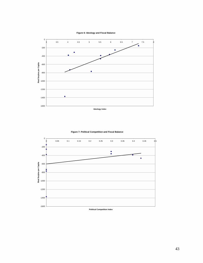
43

Figure 6: Ideology and Fiscal Balance

-1600

-1400

-1200

-1000

-800

-600

-400

-200

03 3.5 4 4.5 5 5.5 6 6.5 7 7.5 8

Ideology Index

Rea

l Sur

plus

per

Cap

ita

Figure 7: Political Competition and Fiscal Balance

-1600

-1400

-1200

-1000

-800

-600

-400

-200

00 0.05 0.1 0.15 0.2 0.25 0.3 0.35 0.4 0.45 0.5

Political Competition Index

Rea

l Sur

plus

per

Cap

ita

44

Over Time Within Länder Across Länder

H1 Grants Support SupportH2 Jurisdiction Size na SupportH3 Business Cycle Opposite naH4 Election Cycle Support naH5 Partisan Business Cycle No Support naH6 Long-term Partisanship na SupportH7 Vertical Partisan Similarity No Support Opposite (Weak)H8 Political Fragmentation Opposite (Weak) No SupportH9 Political Competition No Support No Support

Table 7: Overview of Results

and the last shall be first - mit

Documents