Wireless Communications

Andrea Goldsmith

Draft of Second Edition

Chapters 1-6

Dec. 18, 2019

Contents

1 Overview of Wireless Communications 1

1.1 History of Wireless Communications . . . . . . . . . . . . . . . . . . . . . . . . . . . . . . . . . 1

1.1.1 Origins of Radio Technology . . . . . . . . . . . . . . . . . . . . . . . . . . . . . . . . . 1

1.1.2 From Analog to Digital . . . . . . . . . . . . . . . . . . . . . . . . . . . . . . . . . . . . 2

1.1.3 Evolution of Wireless Systems and Standards . . . . . . . . . . . . . . . . . . . . . . . . 2

1.2 Current Systems . . . . . . . . . . . . . . . . . . . . . . . . . . . . . . . . . . . . . . . . . . . . 7

1.2.1 Wireless Local Area Networks . . . . . . . . . . . . . . . . . . . . . . . . . . . . . . . . 7

1.2.2 Cellular Systems . . . . . . . . . . . . . . . . . . . . . . . . . . . . . . . . . . . . . . . 8

1.2.3 Satellite Systems . . . . . . . . . . . . . . . . . . . . . . . . . . . . . . . . . . . . . . . 11

1.2.4 Fixed Wireless Access . . . . . . . . . . . . . . . . . . . . . . . . . . . . . . . . . . . . 12

1.2.5 Short Range Radios with Multihop Routing . . . . . . . . . . . . . . . . . . . . . . . . . 13

1.3 Wireless Spectrum . . . . . . . . . . . . . . . . . . . . . . . . . . . . . . . . . . . . . . . . . . 14

1.3.1 Regulation . . . . . . . . . . . . . . . . . . . . . . . . . . . . . . . . . . . . . . . . . . 14

1.3.2 Properties and Existing Allocations . . . . . . . . . . . . . . . . . . . . . . . . . . . . . 17

1.4 Communication Standards . . . . . . . . . . . . . . . . . . . . . . . . . . . . . . . . . . . . . . 18

1.5 Wireless Vision . . . . . . . . . . . . . . . . . . . . . . . . . . . . . . . . . . . . . . . . . . . . 19

1.6 Technical Challenges . . . . . . . . . . . . . . . . . . . . . . . . . . . . . . . . . . . . . . . . . 20

2 Path Loss, Shadowing, and Multipath 26

2.1 Radio Wave Propagation . . . . . . . . . . . . . . . . . . . . . . . . . . . . . . . . . . . . . . . 27

2.2 Transmit and Receive Signal Models . . . . . . . . . . . . . . . . . . . . . . . . . . . . . . . . . 28

2.3 Free-Space Path Loss . . . . . . . . . . . . . . . . . . . . . . . . . . . . . . . . . . . . . . . . . 30

2.4 Two-Ray Multipath Model . . . . . . . . . . . . . . . . . . . . . . . . . . . . . . . . . . . . . . 32

2.5 Path Loss Exponent Models . . . . . . . . . . . . . . . . . . . . . . . . . . . . . . . . . . . . . 35

2.5.1 Single-Slope . . . . . . . . . . . . . . . . . . . . . . . . . . . . . . . . . . . . . . . . . 35

2.5.2 Multi-Slope . . . . . . . . . . . . . . . . . . . . . . . . . . . . . . . . . . . . . . . . . . 37

2.6 Shadowing . . . . . . . . . . . . . . . . . . . . . . . . . . . . . . . . . . . . . . . . . . . . . . 38

2.7 Combined Path Loss and Shadowing . . . . . . . . . . . . . . . . . . . . . . . . . . . . . . . . . 42

2.7.1 Single-Slope Path Loss with Log-Normal Shadowing . . . . . . . . . . . . . . . . . . . . 42

2.7.2 Outage Probability . . . . . . . . . . . . . . . . . . . . . . . . . . . . . . . . . . . . . . 42

2.7.3 Cell Coverage Area and Percentage . . . . . . . . . . . . . . . . . . . . . . . . . . . . . 43

2.8 General Ray Tracing . . . . . . . . . . . . . . . . . . . . . . . . . . . . . . . . . . . . . . . . . 46

2.8.1 Multi-Ray Reflections . . . . . . . . . . . . . . . . . . . . . . . . . . . . . . . . . . . . 48

2.8.2 Diffraction . . . . . . . . . . . . . . . . . . . . . . . . . . . . . . . . . . . . . . . . . . 49

2.8.3 Scattering . . . . . . . . . . . . . . . . . . . . . . . . . . . . . . . . . . . . . . . . . . . 51

2.8.4 Multipath Model with Reflection, Diffraction, and Scattering . . . . . . . . . . . . . . . . 51

ii

2.8.5 Multi-Antenna and MIMO Systems . . . . . . . . . . . . . . . . . . . . . . . . . . . . . 52

2.8.6 Local Mean Received Power . . . . . . . . . . . . . . . . . . . . . . . . . . . . . . . . . 52

2.9 Measurement-Based Propagation Models . . . . . . . . . . . . . . . . . . . . . . . . . . . . . . 52

2.9.1 Okumura Model . . . . . . . . . . . . . . . . . . . . . . . . . . . . . . . . . . . . . . . 53

2.9.2 Hata Model . . . . . . . . . . . . . . . . . . . . . . . . . . . . . . . . . . . . . . . . . . 54

2.9.3 Cellular System Models . . . . . . . . . . . . . . . . . . . . . . . . . . . . . . . . . . . 54

2.9.4 Wi-Fi Channel Models . . . . . . . . . . . . . . . . . . . . . . . . . . . . . . . . . . . . 56

2.9.5 Millimeter Wave Models . . . . . . . . . . . . . . . . . . . . . . . . . . . . . . . . . . . 57

2.9.6 Indoor Attentuation Models . . . . . . . . . . . . . . . . . . . . . . . . . . . . . . . . . 59

3 Statistical Multipath Channel Models 73

3.1 Time-Varying Channel Impulse Response . . . . . . . . . . . . . . . . . . . . . . . . . . . . . . 74

3.2 Narrowband Fading Model . . . . . . . . . . . . . . . . . . . . . . . . . . . . . . . . . . . . . . 79

3.2.1 Autocorrelation, Cross-Correlation, and Power Spectral Density . . . . . . . . . . . . . . 80

3.2.2 Envelope and Power Distributions . . . . . . . . . . . . . . . . . . . . . . . . . . . . . . 86

3.2.3 Level Crossing Rate and Average Fade Duration . . . . . . . . . . . . . . . . . . . . . . 89

3.2.4 Block-Fading and Finite-State Markov Fading . . . . . . . . . . . . . . . . . . . . . . . 91

3.3 Wideband Fading Model . . . . . . . . . . . . . . . . . . . . . . . . . . . . . . . . . . . . . . . 92

3.3.1 Autocorrelation and Scattering Function . . . . . . . . . . . . . . . . . . . . . . . . . . . 93

3.3.2 Power Delay Profile . . . . . . . . . . . . . . . . . . . . . . . . . . . . . . . . . . . . . 94

3.3.3 Coherence Bandwidth . . . . . . . . . . . . . . . . . . . . . . . . . . . . . . . . . . . . 97

3.3.4 Doppler Power Spectrum and Channel Coherence Time . . . . . . . . . . . . . . . . . . 99

3.3.5 Transforms for Autocorrelation and Scattering Functions . . . . . . . . . . . . . . . . . . 100

3.4 Discrete-Time Model . . . . . . . . . . . . . . . . . . . . . . . . . . . . . . . . . . . . . . . . . 100

3.5 MIMO Channel Models . . . . . . . . . . . . . . . . . . . . . . . . . . . . . . . . . . . . . . . . 102

4 Capacity of Wireless Channels 111

4.1 Capacity in AWGN . . . . . . . . . . . . . . . . . . . . . . . . . . . . . . . . . . . . . . . . . . 112

4.2 Capacity of Flat Fading Channels . . . . . . . . . . . . . . . . . . . . . . . . . . . . . . . . . . . 114

4.2.1 Channel and System Model . . . . . . . . . . . . . . . . . . . . . . . . . . . . . . . . . 114

4.2.2 Channel Distribution Information Known . . . . . . . . . . . . . . . . . . . . . . . . . . 115

4.2.3 Channel Side Information at Receiver . . . . . . . . . . . . . . . . . . . . . . . . . . . . 115

4.2.4 Channel Side Information at Transmitter and Receiver . . . . . . . . . . . . . . . . . . . 118

4.2.5 Capacity with Receiver Diversity . . . . . . . . . . . . . . . . . . . . . . . . . . . . . . 124

4.2.6 Capacity Comparisons . . . . . . . . . . . . . . . . . . . . . . . . . . . . . . . . . . . . 125

4.3 Capacity of Frequency-Selective Fading Channels . . . . . . . . . . . . . . . . . . . . . . . . . . 126

4.3.1 Time-Invariant Channels . . . . . . . . . . . . . . . . . . . . . . . . . . . . . . . . . . . 126

4.3.2 Time-Varying Channels . . . . . . . . . . . . . . . . . . . . . . . . . . . . . . . . . . . 129

5 Digital Modulation and Detection 138

5.1 Signal Space Analysis . . . . . . . . . . . . . . . . . . . . . . . . . . . . . . . . . . . . . . . . . 139

5.1.1 Signal and System Model . . . . . . . . . . . . . . . . . . . . . . . . . . . . . . . . . . 139

5.1.2 Geometric Representation of Signals . . . . . . . . . . . . . . . . . . . . . . . . . . . . . 140

5.1.3 Receiver Structure and Sufficient Statistics . . . . . . . . . . . . . . . . . . . . . . . . . 144

5.1.4 Decision Regions and the Maximum Likelihood Decision Criterion . . . . . . . . . . . . 146

5.1.5 Error Probability and the Union Bound . . . . . . . . . . . . . . . . . . . . . . . . . . . 148

5.2 Passband Modulation Principles . . . . . . . . . . . . . . . . . . . . . . . . . . . . . . . . . . . 153

5.3 Amplitude and Phase Modulation . . . . . . . . . . . . . . . . . . . . . . . . . . . . . . . . . . 153

5.3.1 Pulse Amplitude Modulation (MPAM) . . . . . . . . . . . . . . . . . . . . . . . . . . . . 155

5.3.2 Phase-Shift Keying (MPSK) . . . . . . . . . . . . . . . . . . . . . . . . . . . . . . . . . 157

5.3.3 Quadrature Amplitude Modulation (MQAM) . . . . . . . . . . . . . . . . . . . . . . . . 159

5.3.4 Differential Modulation . . . . . . . . . . . . . . . . . . . . . . . . . . . . . . . . . . . 160

5.3.5 Constellation Shaping . . . . . . . . . . . . . . . . . . . . . . . . . . . . . . . . . . . . 163

5.3.6 Quadrature Offset . . . . . . . . . . . . . . . . . . . . . . . . . . . . . . . . . . . . . . . 163

5.4 Frequency Modulation . . . . . . . . . . . . . . . . . . . . . . . . . . . . . . . . . . . . . . . . 163

5.4.1 Frequency-Shift Keying (FSK) and Minimum-Shift Keying (MSK) . . . . . . . . . . . . 164

5.4.2 Continuous-Phase FSK (CPFSK) . . . . . . . . . . . . . . . . . . . . . . . . . . . . . . 165

5.4.3 Noncoherent Detection of FSK . . . . . . . . . . . . . . . . . . . . . . . . . . . . . . . . 166

5.5 Pulse Shaping . . . . . . . . . . . . . . . . . . . . . . . . . . . . . . . . . . . . . . . . . . . . . 167

5.6 Symbol Synchronization and Carrier Phase Recovery . . . . . . . . . . . . . . . . . . . . . . . . 170

5.6.1 Receiver Structure with Phase and Timing Recovery . . . . . . . . . . . . . . . . . . . . 171

5.6.2 Maximum Likelihood Phase Estimation . . . . . . . . . . . . . . . . . . . . . . . . . . . 173

5.6.3 Maximum Likelihood Timing Estimation . . . . . . . . . . . . . . . . . . . . . . . . . . 174

6 Performance of Digital Modulation over Wireless Channels 182

6.1 AWGN Channels . . . . . . . . . . . . . . . . . . . . . . . . . . . . . . . . . . . . . . . . . . . 182

6.1.1 Signal-to-Noise Power Ratio and Bit/Symbol Energy . . . . . . . . . . . . . . . . . . . . 182

6.1.2 Error Probability for BPSK and OPSK . . . . . . . . . . . . . . . . . . . . . . . . . . . . 183

6.1.3 Error Probability for MPSK . . . . . . . . . . . . . . . . . . . . . . . . . . . . . . . . . 185

6.1.4 Error Probability for MPAM and MQAM . . . . . . . . . . . . . . . . . . . . . . . . . . 186

6.1.5 Error Probability for FSK and CPFSK . . . . . . . . . . . . . . . . . . . . . . . . . . . . 188

6.1.6 Error Probability Approximation for Coherent Modulations . . . . . . . . . . . . . . . . 189

6.1.7 Error Probability for Differential Modulation . . . . . . . . . . . . . . . . . . . . . . . . 190

6.2 Alternate Q-Function Representation . . . . . . . . . . . . . . . . . . . . . . . . . . . . . . . . 191

6.3 Fading . . . . . . . . . . . . . . . . . . . . . . . . . . . . . . . . . . . . . . . . . . . . . . . . . 192

6.3.1 Outage Probability . . . . . . . . . . . . . . . . . . . . . . . . . . . . . . . . . . . . . . 192

6.3.2 Average Probability of Error . . . . . . . . . . . . . . . . . . . . . . . . . . . . . . . . . 193

6.3.3 Moment Generating Function Approach to Average Error Probability . . . . . . . . . . . 196

6.3.4 Combined Outage and Average Error Probability . . . . . . . . . . . . . . . . . . . . . . 200

6.4 Doppler Spread . . . . . . . . . . . . . . . . . . . . . . . . . . . . . . . . . . . . . . . . . . . . 201

6.5 Intersymbol Interference . . . . . . . . . . . . . . . . . . . . . . . . . . . . . . . . . . . . . . . 203

0

Chapter 1

Overview of Wireless Communications

Wireless communication is one of the most impactful technologies in history, drastically affecting the way we live,

work, play, and interact with people and the world. There are billions of cellphone subscribers worldwide, and

a wide range of devices in addition to phones use cellular technology for their connectivity. Wireless network

technology using the Wi-Fi standard has been incorporated into billions of devices as well, including smartphones,

computers, cars, drones, kitchen appliances, watches, and tennis shoes. Satellite communication systems support

video, voice, and data applications for receivers on earth, in the air, and in space. Revenue across all areas of

wireless technology and services is trillions of dollars annually. The insatiable demand for wireless data along

with new and compelling wireless applications indicate a bright future for wireless systems. However, many

technical challenges remain in designing wireless networks and devices that deliver the performance necessary

to support existing and emerging applications. In this introductory chapter we will briefly review the history of

wireless communications, from the smoke signals of antiquity to the rise of radio communication that underlies

the Wi-Fi, cellular, and satellite networks of today. We then discuss the most prevalent wireless communication

systems in operation today. The impact of spectrum properties and regulation as well as standards on the design

and success of wireless systems is also illuminated. We close the chapter by presenting a vision for the wireless

communication systems of the future, including the technical challenges that must be overcome to make this

vision a reality. Techniques to address many of these challenges are covered in subsequent chapters. The huge

gap between the capabilities of current systems and the vision for future systems indicates that much research and

development in wireless communications remains to be done.

1.1 History of Wireless Communications

1.1.1 Origins of Radio Technology

The first wireless networks were developed in antiquity. These systems transmitted information visually over

line-of-sight distances (later extended by telescopes) using smoke signals, torch signaling, flashing mirrors, signal

flares, or semaphore flags. An elaborate set of signal combinations was developed to convey complex messages

with these rudimentary signals. Observation stations were built on hilltops and along roads to relay these messages

over large distances. These early communication networks were replaced first by the telegraph network (invented

by Samuel Morse in 1838) and later by the telephone.

The origins of radio communications began around 1820 with experiments by Oersted demonstrating that an

electric field could move a compass needle, thereby establishing a connection between electricity and magnetism.

Work by Ampere, Gauss, Henry, Faraday, and others further advanced knowledge about electromagnetic waves,

culminating in Maxwell’s theory of electromagnetism published in 1865. The first transmission of electromagnetic

1

waves was performed by Hertz in the late 1880s, after which he famously declared to his students that these waves

would be “of no use whatsoever.” He was proved wrong in 1895 when Marconi demonstrated the first radio trans-

mission across his father’s estate in Bologna. That transmission is considered the birth of radio communications,

a term coined in the early 1900s. Marconi moved to England to continue his experiments over increasingly large

transmission ranges, culminating in the first trans-Atlantic radio transmission in 1901. In 1900 Fessenden became

the first person to send a speech signal over radio waves, and six years later he made the first public radio broad-

cast. From these early beginnings, described in more detail in [1], radio technology advanced rapidly to enable

transmissions over larger distances with better quality, less power, and smaller, cheaper devices, thereby enabling

public and private radio communications, television, and wireless networking.

1.1.2 From Analog to Digital

Radio systems designed prior to the invention of the transistor, including AM/FM radio, analog television, and

amateur radio, transmitted analog signals. Most modern radio systems transmit digital signals generated by digital

modulation of a bit stream. The bit stream may represent binary data (e.g., a computer file, digital photo, or digital

video stream) or it may be obtained by digitizing an analog signal (e.g., by sampling the analog signal and then

quantizing each sample). A digital radio can transmit a continuous bit stream or it can group the bits into packets.

The latter type of radio is called a packet radio and is characterized by bursty transmissions: the radio is idle

except when it transmits a packet. When packet radios transmit continuous data such as voice and video, the delay

between received packets must not exceed the delay constraint of the data. The first wireless network based on

packet radio, ALOHAnet, was developed at the University of Hawaii and began operation in 1971. This network

enabled computer sites at seven campuses spread out over four islands to communicate with a central computer

on Oahu via radio transmission. The network architecture used a star topology with the central computer at its

hub. Any two computers could establish a bi-directional communications link between them by going through

the central hub. ALOHAnet incorporated the first set of protocols for channel access and routing in packet radio

systems, and many of the underlying principles in these protocols are still in use today.

The U.S. military saw great potential for communication systems exploiting the combination of packet data

and broadcast radio inherent to ALOHAnet. Throughout the 70’s and early 80’s the Defense Advanced Research

Projects Agency (DARPA) invested significant resources to develop networks using packet radios for communi-

cations in the battlefield. The nodes in these packet radio networks had the ability to configure (or reconfigure)

into a network without the aid of any established infrastructure. Self-configuring wireless networks without any

infrastructure were later coined ad hoc wireless networks.

DARPA’s investment in packet radio networks peaked in the mid 1980’s, but these networks fell far short of

expectations in terms of speed and performance. This was due in part to the limited capabilities of the radios and in

part to the lack of robust and efficient access and routing protocols. Packet radio networks also found commercial

application in supporting wide-area wireless data services. These services, first introduced in the early 1990’s,

enabled wireless data access (including email, file transfer, and web browsing) at fairly low speeds, on the order

of 20 Kbps. The market for these wide-area wireless data services did not take off due mainly to their low data

rates, high cost, and lack of “killer applications”. All of these services eventually folded, spurred in part by the

introduction of wireless data in 2G cellular services [2], which marked the dawn of the wireless data revolution.

1.1.3 Evolution of Wireless Systems and Standards

The ubiquity of wireless communications has been enabled by the growth and success of Wireless Local Area Net-

works (WLANs), standardized through the family of IEEE 802.11 (Wi-Fi) protocols, as well as cellular networks.

Satellite systems also play an important role in the wireless ecosystem. The evolution of these systems and their

corresponding standards is traced out in this subsection.

2

Wi-Fi Systems

The success story of Wi-Fi systems, as illuminated in [3], began as an evolution of the Ethernet (802.3)

standard for wired local area networks (LANs). Ethernet technology, developed at Xerox Parc in the 1970s and

standardized in 1983, was widely adopted throughout the 1980s to connect computers, servers, and printers within

office buildings. WLANs were envisioned as Ethernet LANs with cables replaced by radio links. In 1985 the

Federal Communications Commission (FCC) enabled the commercial development of WLANs by authorizing for

unlicensed use three of the Industrial, Scientific, and Medical (ISM) frequency bands: the 900 MHz band spanning

902-928 MHz, the 2.4 GHz band spanning 2.4-2.4835 GHz, and the 5.8 GHz band spanning 5.725-5.875 GHz. Up

until then, these frequency bands had been reserved internationally for radio equipment associated with industrial,

scientific and medical purposes other than telecommunications. Similar rulings followed shortly thereafter from

the spectrum regulatory bodies in other countries. The new rulings allowed unlicensed use of these ISM bands by

any radio following a certain set of restrictions to avoid compromising the performance of the primary band users.

Such radios were also subject to interference from these primary users. The opening of these ISM bands to “free”

use by unlicensed wireless devices unleashed a flurry of research and commercial wireless system development,

particularly for WLANs.

The first WLAN product for the ISM band, called WaveLAN, was launched in 1988 by the NCR corporation

and cost several thousand dollars. These WLANs had data rates up to 2 Mbps and operated in the 900 MHz and

2.4 GHz ISM bands. Dozens of WLAN companies and products appeared over the ensuing few years, mostly

operating in the 900 MHz ISM band using direct-sequence spread spectrum, with data rates on the order of 1-

2 Mbps. The lack of standardization for these products led to high development costs, poor reliability, and lack

of interoperability between systems. Moreover, Ethernet’s 10 Mbps data rate and high reliability far exceeded the

capabilities of these early WLAN products. Since companies were willing to run cables within and between their

facilities to get this better performance, the WLAN market remained small for its first decade of existence. The

initial WLAN products were phased out as the 802.11 standards-based WLAN products hit the market in the late

1990s. In Europe a WLAN standard called HIPERLAN was finalized in 1996. An improved version was launched

in 2000, but HIPERLAN systems never gained much traction.

The first 802.11 standard, finalized in 1997, was born from a working group within the IEEE 802 LAN/MAN

Standards Committee that was formed in 1990. This standard, called 802.11-1997, operated in the 2.4 GHz ISM

band with data rates up to 2 Mbps. The standard used channel sensing with collision avoidance for medium access

as well as frequency hopping or direct-sequence spread spectrum to mitigate the main sources of interference in

that band which, at the time, consisted primarily of microwave ovens, cordless phones, and baby monitors. Also in

1997, the FCC authorized 200 MHz of additional unlicensed spectrum in the 5 GHz band, with certain constraints

to avoid interfering with the primary users, mostly radar systems, operating in this band. Two years later, in 1999,

the standard that would ignite the Wi-Fi revolution, 802.11b, was finalized. This standard increased data rates to 11

Mbps and eliminated the frequency-hop option of its predecessor. A plethora of 802.11b products soon appeared.

Their interoperability, coupled with dramatically lower costs relative to earlier WLAN products, led to widespread

use of this new technology. Millions of 802.11b products were shipped in 2000, just one year after the standard was

finalized, and these shipments grew tenfold by 2003. The year 1999 marked two other important milestones for

WLANs. That year the 802.11a standard for the 5GHz ISM frequency band was finalized to capitalize on the new

unlicensed spectrum in that band. This standard enabled 54 Mbps data rates in 20 MHz channels and introduced

orthogonal-frequency-division-multiplexing (OFDM) coupled with adaptive modulation as a new physical layer

design. Also in 1999 the Wireless Ethernet Compatibility Alliance was formed to facilitate interoperability and

certification of WLAN products. The name of this group was later abbreviated to the Wi-Fi Alliance, thereby

coining the widely used moniker for WLAN technology and standards today.

3

The Wi-Fi standard has evolved rapidly since its early days, with new versions developed about every five

years, as described in more detail in Appendix D.1. The 802.11g standard, introduced in 2003, is essentially the

same in its physical layer and multiple access design as 802.11a, but operates in the 2.4 GHz ISM frequency

band. Later standards provided improvements over these first OFDM Wi-Fi systems, including wider channels,

multiple transmit and receive antennas to enable multiple spatial streams and improved robustness through beam-

forming, larger signal constellations, improved error-correction codes, and coordinated multiple access. These

improvements have led to highly-reliable Wi-Fi products that are capable of 10 Gbps data rates within a building

or outdoor area. Wi-Fi has also moved into the unregulated 60 GHz frequency band through the 802.11ad standard.

Even its name has evolved; In 2018 the 802.11 standards body abandoned using letter suffixes for new generations

of the standard. Instead it coined the sixth generation of the WiFi standard, originally named 802.11ax, as Wi-Fi

6. Today Wi-Fi technology is pervasive indoors and out even in remote corners of the world. In addition to its

pervasiveness, Wi-Fi has experienced an explosion of applications beyond its original use of connecting computers

to each other and their peripheral devices. In addition to computers, smartphones, and tablets, many electronic

devices today, from medical devices to refrigerators to cars, are equipped with Wi-Fi, allowing them to download

new software, exchange data with other devices, and take advantage of cloud-based storage and computation.

Cellular Systems

Cellular systems are another exceedingly successful wireless technology. The convergence of radio and tele-

phony began in 1915, when wireless voice transmission between New York and San Francisco was first established.

The first analog mobile telephone system was deployed in St. Louis Missouri in 1946, launching AT&T’s Mobile

Telephone Service (MTS). Within two years AT&T had deployed MTS over approximately 100 cities and highway

corridors. Only six channels were allocated by the FCC for the service and, due to their close spacing in frequency,

only three were usable at any given time. Hence only three people within a city could make a call simultaneously.

The monthly service and per-call cost was very high, and the equipment bulky and heavy. Evolution of the system

was slow; while the equipment improved and spectrum to support up to 12 channels was added, the system capacity

remained extremely limited.

Ironically, about the same time MTS was first being deployed, a solution to this capacity problem had already

emerged from researchers at AT&T Bell Laboratories: the notion of cellular systems. The cellular system concept,

articulated in a 1947 Bell Laboratories Technical Memo by D. H. Ring [4], exploited the fact that the power of

a transmitted signal falls off with distance. Thus, channels using the same frequency can be allocated to users at

spatially-separate locations with minimal interference between the users. To exploit this principle of frequency

reuse, a cellular system partitions a geographical area into non-overlapping cells, as shown in Fig. 1.3 below. Sets

of channels are assigned to each cell, and cells that are assigned the same channel set are spaced far enough apart

so that interference between the users in these cells is small. In early cellular systems the distance between cells

using the same channel set was relatively large, but today sophisticated interference mitigation techniques allow

channels to be reused in every cell. As a user moves between adjacent cells, its call is handed off to a channel

associated with the new cell. Frequency reuse enables much more efficient use of spectrum as the number of

simultaneous users is no longer limited to the number of available channels. Indeed, while many aspects of cellular

system technology have changed over time, frequency reuse remains at the heart of cellular system design.

Although the cellular concept was introduced in the late 1940s, it was not implemented for several decades,

as technology was not yet ripe to realize the system in practice. In the mid-1960s engineers at Bell Laboratories

began work on a design and feasibility study for a metropolitan analog cellular system. The details of the design

and analysis, along with successful system tests in Newark and Philadelphia, formed the basis of an AT&T FCC

proposal in 1971 to approve cellular service and allocate spectrum for it [5]. The FCC approved experimental

cellular licenses to telephone companies in 1974, which led to the construction of several cellular systems. Fol-

4

lowing a long and convoluted process, in 1981 the FCC finalized its ruling for the issuance of commercial cellular

licenses, instituting a duopoly in every metropolitan area whereby one license would be granted to a traditional

phone company, and the other to a non-traditional operator. The first generation cellular system for U.S. deploy-

ment, called the advanced mobile phone system (AMPS) and described in [6], was launched in Chicago in 1983.

A similar service had been launched in Tokyo in 1979 and in Scandinavia in 1981, although those systems were

incompatible with AMPS. Cellular service in many other countries launched in the ensuing years, mostly with

incompatible standards, which precluded cellular roaming between countries. These first generation systems are

referred to as 1G systems.

Like Wi-Fi, the exponential growth of the cellular industry exceeded all expectations, increasing by at least

an order of magnitude every decade, from a modest 100,000 subscribers in 1984 to tens of millions in 1994,

hundreds of millions in 2004, and billions in 2014. To meet the growing demand for wireless data along with a

diverse requirements for different types of wireless devices, a new generation of cellular systems and standards

has emerged approximately every decade. In fact, that timeline was compressed for 1G systems, since the analog

cellular system deployed in Chicago in 1983 was already saturated by 1984. At that point the FCC increased the

cellular spectral allocation from 40 MHz to 50 MHz. As cellular systems throughout more and more cities became

saturated with demand, the development of digital cellular technology for increased capacity and better perfor-

mance became essential. These enhanced system requirements launched the process to create a second generation

(2G) cellular standard in the late 1980s with deployments in the early 1990s. In addition to voice communication,

the move to digital technology paved the way for these systems to support low-rate data as well, in particular

short texts, voice mail, and paging services. Unfortunately, the great market potential for cellular phones led to a

proliferation of 2G cellular standards, with three different standards in the U.S. alone. One of these matched the

European standard; Japan adopted a separate standard. Hence global roaming required a multi-mode phone. This

deficiency was corrected for the third generation of cellular standards (3G), for which seven telecommunications

standards bodies across Asia, Europe and the United States formed the third-generation partnership project (3GPP)

to develop a single worldwide standard. The 3G cellular systems based on the 3GPP standard, whose deployments

began in the early 2000s, provided an order of magnitude higher peak data rates than 2G systems. Indeed, it was

the capabilities of 3G systems that transitioned the “killer application” of cell phones from voice to wireless data.

The proliferation of smart phone technology in the mid-2000s, which were designed to consume vast amounts of

wireless data, greatly stressed the capacity of 3G networks. Moreover, the 3G networks had far lower data rates

than Wi-Fi, which became the access mode of choice for high-speed data. These developments paved the way for

the next-generation 4G “long term evolution (LTE)” cellular standard. These systems, deployed in the early 2010s,

supported an order-of-magnitude peak data rate increase over 3G systems. The 5G cellular standard supports

higher data rates than 4G systems, as well as lower latency and better energy efficiency. System deployments for

5G began in 2019, continuing the trend of new cellular systems and standards every decade. Starting with the 3G

systems, each generation of cellular standard has been developed to meet a set of International Mobile Telecom-

munications (IMT) requirements outlined by the International Telecommunications Union (ITU). The ITU certifies

which cellular standards meet its IMT requirements; the 3GPP standard is designed to meet these requirements, as

are alternate standards developed by specific countries or other standards organizations. More details on current

cellular technology will be given in Chapter 15, with the evolution of cellular standards described in Appendix D.2.

Satellite Systems

Satellite communication systems are another major component of today’s wireless communications infras-

tructure. Commercial satellite systems can provide broadcast services over very wide areas, fill the coverage gap

in locations without cellular service, and provide connectivity for aerial systems such as airplane Wi-Fi. Satellite

systems are typically categorized by the height of the satellites’ orbit: low-earth orbit (LEO) satellites operate at

5

roughly 2000 km altitude, medium-earth orbit (MEO) satellites at roughly 9000 km altitude, and geosynchronous

orbit (GEO) satellites at roughly 40,000 km altitude. GEO satellites with geostationary orbits are seen as station-

ary from the earth, whereas GEO satellites with other orbits (such as elliptical) have their coverage area change

over time. The disadvantage of high altitude orbits is that it takes a great deal of power to reach the satellite,

and the propagation delay is typically too large for two-way delay-constrained applications like voice, video, and

gaming. However, satellites at these orbits tend to have larger coverage areas, so fewer satellites are necessary to

provide wide-area or global coverage. In addition to communication services, satellites are used for many other

applications including weather monitoring, earth observation, surveillance, imaging, navigation, and localization.

The concept of using GEO satellites for communications was first suggested by Herman Potocnik in 1928 and

later popularized through a 1945 article in Wireless World written by the science fiction writer Arthur C. Clarke.

However, the first deployed satellites, the Soviet Union’s Sputnik in 1957 and the Nasa/Bell Laboratories’ Echo-1

in 1960, were not geosynchronous due to the difficulty of lifting a satellite into such a high orbit. Following these

launches, in 1962 the Communications Satellite Corporation (Comsat) was formed in the United States to develop

commercial communication satellite systems. Two years later, the International Telecommunications Satellite

Consortium (IntelSat) emerged as a public-private consortium of 18 countries with the goal of enabling global

telecommunications connectivity. SYNCOM 2, the first communication satellite to successfully reach geosyn-

chronous orbit, was launched in 1963. The following year SYNCOM 3 was launched into geostationary orbit,

providing a two-way 10 MHz communication channel at a carrier frequency of 1.8 GHz for the satellite-to-earth

link (downlink) and at 7.3 GHz for the reverse link (uplink). Shortly after its launch, SYNCOM 3 was used to

provide live television coverage to US viewers of the 1964 Summer Olympics in Tokyo. The IntelSat consortium

launched a number of satellites during the late 1960s in order to reach near-global coverage, culminating in the

broadcasting of the 1969 landing of the first human on the moon to 600 million viewers. In addition to television

broadcasting, these early systems also supported voice, teletype, and paging.

GEO satellite technology has evolved continuously since its early days. The C band of the radio spectrum

(4-8 GHz) was used in early GEO systems, but subsequent systems have taken advantage of the larger bandwidths

available at the higher frequency X (8-12.5 GHz), Ku (12.5-18 GHz), and Ka (26.5-40 GHz) bands in order to

provide higher data rates. Antenna system technology for GEOs has also evolved to focus the transmission energy

more precisely, leading to higher signal quality and hence higher data rates. There are hundreds of GEO satellites

deployed today, with some capable of a total data rate in excess of one hundred Gbps. For individual users, typical

data rates are on the order of ten Mbps in the downlink and several Mbps in the uplink [7]. Due to their large

coverage regions, geosynchronous satellites are the primary communications mechanism for vessels at sea and in

the air. They are also well-suited for broadcast entertainment where round-trip delay is not a consideration; they

support hundreds of channels of digital television and radio at very high quality.

As cellular systems were rolled out in the late 1980s, the focus for satellite technology turned to building LEO

systems that might compete with them. This led to the launch of several LEO communication systems in the late

1990s, including Globalstar and Iridium [8]. These LEOs provided global coverage but the link rates remained

low due to power and bandwidth constraints. The handsets for these systems were also much larger and heavier

than their cellular counterparts, primarily due to their large batteries. The LEO satellite systems deployed in the

1990s did not experience significant commercial success as, for most users, they provided worse performance

and coverage than the competing 2G cellular phone technology at a higher cost. While these satellite systems

provided coverage to remote areas without access to cellular service, the cost was prohibitive for the large majority

of people in these areas. As a result, pretty much all the initial LEO companies, including Globalstar and Iridium,

filed for bankruptcy protection within a few years of launching their service. Teledesic, which was planning a very

ambitious LEO system with more than 800 satellites, declared bankrupcy before a single launch. After several

iterations of restructuring, Iridium and Globalstar emerged as profitable services and today provide global Internet

connectivity, albeit for a relatively small number of subscribers compared to that of cellular service. Interest in

6

LEO satellites resurfaced as 4G cellular systems rolled out due to increased demand for connectivity in remote

locations not served by cellular, better technology for both satellites and ground transceivers, and reduced launch

costs. Significant commercial development of LEO satellites emerged concurrent with 5G cellular rollouts as a

means to provide broadband Internet service to the billions of people worldwide that do not have access to high-

speed connectivity. It is anticipated that such systems will each deploy hundreds to thousands of satellites.

Today we take for granted the magic of wireless communications, which allows us and our devices to be

connected anywhere in the world. This magic has been enabled by the pioneers that contributed to advances in

wireless technology underlying the powerful systems ubiquitous today.

1.2 Current Systems

This section provides a design overview of the most prevalent wireless systems in operation today. The design

details of these systems are constantly evolving, incorporating new technologies and innovations. This section

will focus mainly on the high-level design aspects of these systems. More details on these systems and their

underlying technologies will be provided in specific sections of the book. A summary of Wi-Fi, cellular, and

short-range networking standards can be found in Appendix D with more complete treatments of recent standards

in [9, 10, 11, 12, 13].

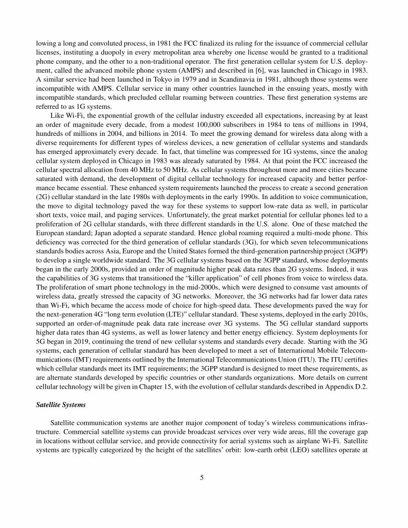
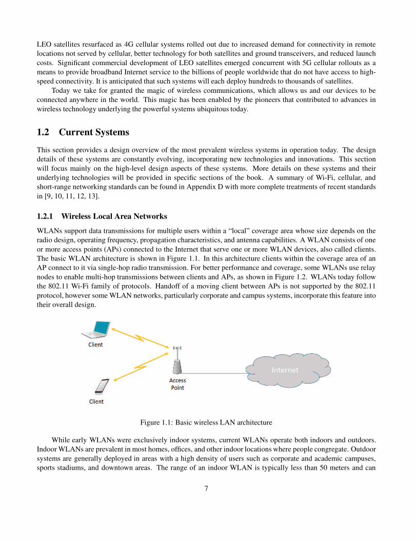
1.2.1 Wireless Local Area Networks

WLANs support data transmissions for multiple users within a “local” coverage area whose size depends on the

radio design, operating frequency, propagation characteristics, and antenna capabilities. A WLAN consists of one

or more access points (APs) connected to the Internet that serve one or more WLAN devices, also called clients.

The basic WLAN architecture is shown in Figure 1.1. In this architecture clients within the coverage area of an

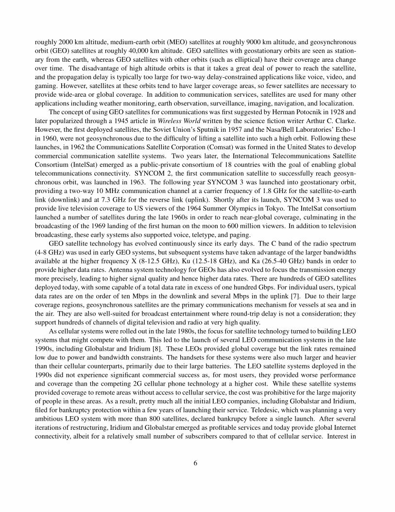
AP connect to it via single-hop radio transmission. For better performance and coverage, some WLANs use relay

nodes to enable multi-hop transmissions between clients and APs, as shown in Figure 1.2. WLANs today follow

the 802.11 Wi-Fi family of protocols. Handoff of a moving client between APs is not supported by the 802.11

protocol, however some WLAN networks, particularly corporate and campus systems, incorporate this feature into

their overall design.

Figure 1.1: Basic wireless LAN architecture

While early WLANs were exclusively indoor systems, current WLANs operate both indoors and outdoors.

Indoor WLANs are prevalent in most homes, offices, and other indoor locations where people congregate. Outdoor

systems are generally deployed in areas with a high density of users such as corporate and academic campuses,

sports stadiums, and downtown areas. The range of an indoor WLAN is typically less than 50 meters and can

7

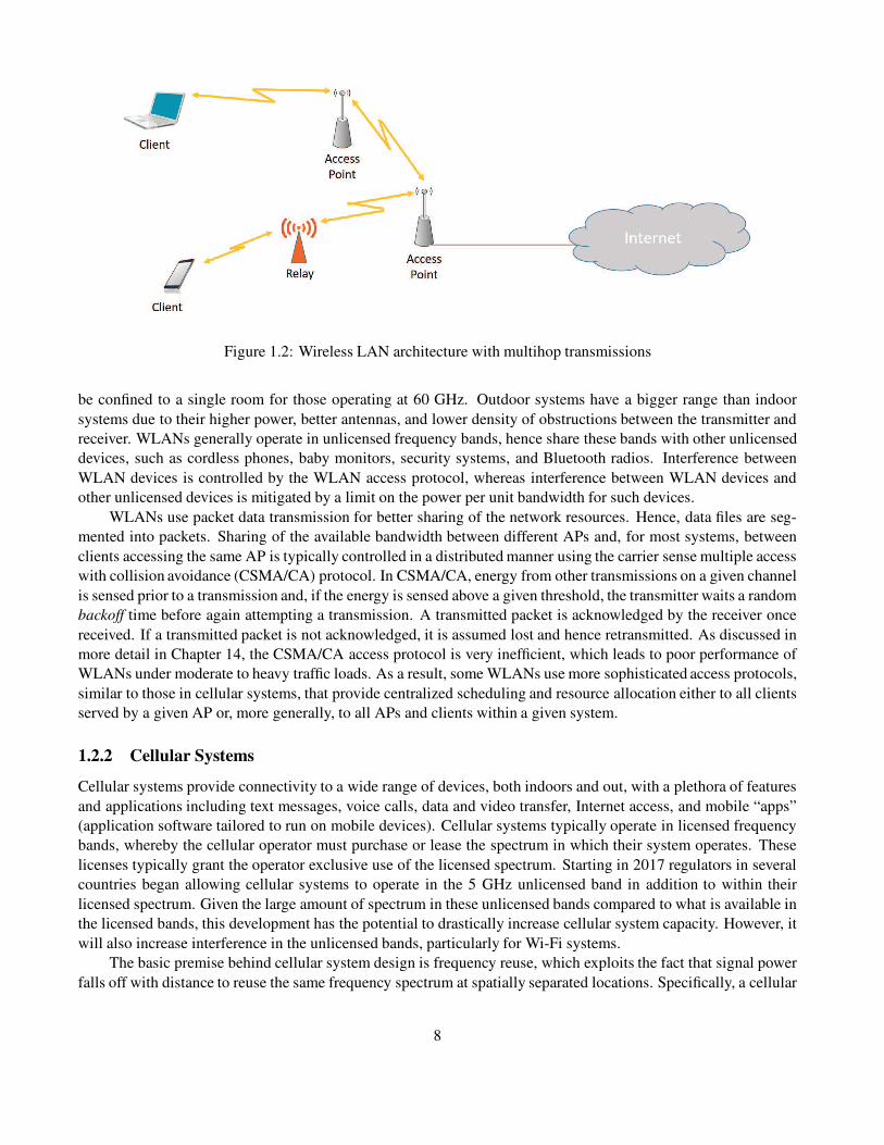
Figure 1.2: Wireless LAN architecture with multihop transmissions

be confined to a single room for those operating at 60 GHz. Outdoor systems have a bigger range than indoor

systems due to their higher power, better antennas, and lower density of obstructions between the transmitter and

receiver. WLANs generally operate in unlicensed frequency bands, hence share these bands with other unlicensed

devices, such as cordless phones, baby monitors, security systems, and Bluetooth radios. Interference between

WLAN devices is controlled by the WLAN access protocol, whereas interference between WLAN devices and

other unlicensed devices is mitigated by a limit on the power per unit bandwidth for such devices.

WLANs use packet data transmission for better sharing of the network resources. Hence, data files are seg-

mented into packets. Sharing of the available bandwidth between different APs and, for most systems, between

clients accessing the same AP is typically controlled in a distributed manner using the carrier sense multiple access

with collision avoidance (CSMA/CA) protocol. In CSMA/CA, energy from other transmissions on a given channel

is sensed prior to a transmission and, if the energy is sensed above a given threshold, the transmitter waits a random

backoff time before again attempting a transmission. A transmitted packet is acknowledged by the receiver once

received. If a transmitted packet is not acknowledged, it is assumed lost and hence retransmitted. As discussed in

more detail in Chapter 14, the CSMA/CA access protocol is very inefficient, which leads to poor performance of

WLANs under moderate to heavy traffic loads. As a result, some WLANs use more sophisticated access protocols,

similar to those in cellular systems, that provide centralized scheduling and resource allocation either to all clients

served by a given AP or, more generally, to all APs and clients within a given system.

1.2.2 Cellular Systems

Cellular systems provide connectivity to a wide range of devices, both indoors and out, with a plethora of features

and applications including text messages, voice calls, data and video transfer, Internet access, and mobile “apps”

(application software tailored to run on mobile devices). Cellular systems typically operate in licensed frequency

bands, whereby the cellular operator must purchase or lease the spectrum in which their system operates. These

licenses typically grant the operator exclusive use of the licensed spectrum. Starting in 2017 regulators in several

countries began allowing cellular systems to operate in the 5 GHz unlicensed band in addition to within their

licensed spectrum. Given the large amount of spectrum in these unlicensed bands compared to what is available in

the licensed bands, this development has the potential to drastically increase cellular system capacity. However, it

will also increase interference in the unlicensed bands, particularly for Wi-Fi systems.

The basic premise behind cellular system design is frequency reuse, which exploits the fact that signal power

falls off with distance to reuse the same frequency spectrum at spatially separated locations. Specifically, a cellular

8

system consists of multiple cells, where each cell is assigned one or more channels to serve its users. Each channel

may be reused in another cell some distance away, and the interference between cells operating on the same

channel is called intercell interference. The spatial separation of cells that reuse the same channel set, the reuse

distance, should be as small as possible so that frequencies are reused as often as possible, thereby maximizing

spectral efficiency. However, as the reuse distance decreases, the intercell interference increases owing to the

smaller propagation distance between interfering cells. Early cellular systems had reuse distances greater than one,

but current systems typically reuse each channel in every cell while managing the resulting interference through

sophisticated mitigation techniques.

The most basic cellular system architecture consists of tessellating cells, as shown in Figure 1.3, where Cidenotes the channel set assigned to cell i. The two-dimensional cell shapes that tessellate (cover a region without

gaps or overlap) are hexagons, squares, and triangles. Of these, the hexagon best approximates an idealized omni-

directional transmitter’s circular coverage area. Early cellular systems followed this basic architecture using a

relatively small number of cells to cover an entire city or region. The cell base stations in these systems were

placed on tall buildings or mountains and transmitted at very high power with cell coverage areas of several square

miles. These large cells are called macrocells. The first few generations of macrocell base stations used single-

antenna omni-directional transmitters, so a mobile moving in a circle around these base station had approximately

constant average received power unless the signal was blocked by an attenuating object. In deployed systems cell

coverage areas overlap or have gaps as signal propagation from a set of base stations never creates tessellating

shapes in practice, even if they can be optimally placed. Optimal base station placement is also impractical, as

zoning restrictions, rooftop availability, site cost, backhaul and power availability, as well as other considerations

influence this placement.

Figure 1.3: Cellular network architecture (homogeneous cell size).

Macrocells have the benefit of wide area coverage, but they can often become overloaded when they contain

more users than channels. This phenomenon has led to hierarchical cellular system architectures, with macrocells

that provide wide area coverage and small cells embedded within these larger cells to provide high capacity, as

shown in Figure 1.4. Not only do the small cells provide increased capacity over a macrocell-only network,

but they also reduce the transmit power required at both the base station and mobile terminal, since the maximum

transmission distance within the small cell is much less than in the macrocell. Cellular systems with heterogeneous

cells sizes are referred to as Hetnets. In current cellular systems, channels are typically assigned dynamically

based on interference conditions. Another feature of many current cellular system designs is for base stations in

adjacent macrocells to operate on the same frequency, utilizing power control, adaptive modulation and coding, as

well as interference mitigation techniques to ensure the interference between users does not preclude acceptable

performance.

All base stations in a given geographical area, both macrocells and small cells, are connected via a high-speed

9

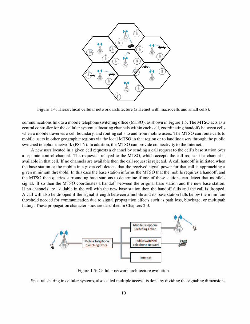
Figure 1.4: Hierarchical cellular network architecture (a Hetnet with macrocells and small cells).

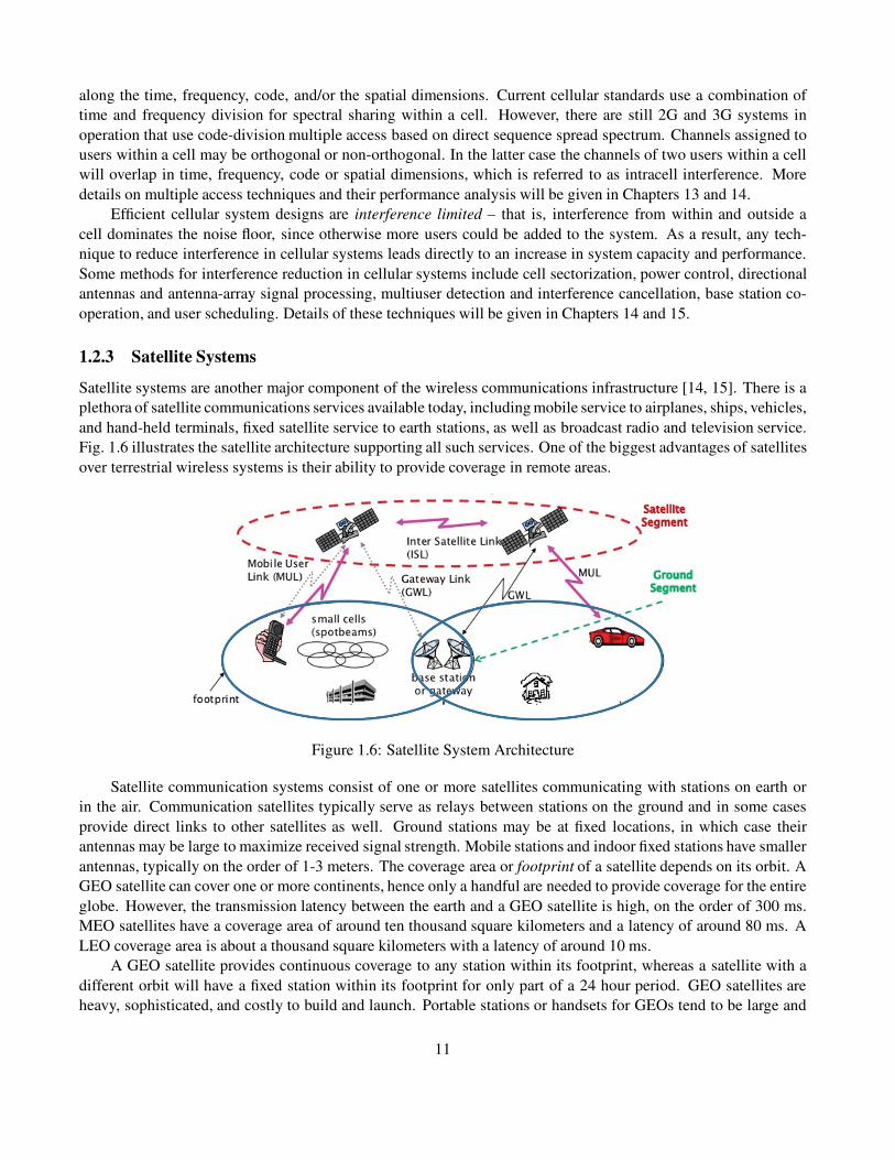
communications link to a mobile telephone switching office (MTSO), as shown in Figure 1.5. The MTSO acts as a

central controller for the cellular system, allocating channels within each cell, coordinating handoffs between cells

when a mobile traverses a cell boundary, and routing calls to and from mobile users. The MTSO can route calls to

mobile users in other geographic regions via the local MTSO in that region or to landline users through the public

switched telephone network (PSTN). In addition, the MTSO can provide connectivity to the Internet.

A new user located in a given cell requests a channel by sending a call request to the cell’s base station over

a separate control channel. The request is relayed to the MTSO, which accepts the call request if a channel is

available in that cell. If no channels are available then the call request is rejected. A call handoff is initiated when

the base station or the mobile in a given cell detects that the received signal power for that call is approaching a

given minimum threshold. In this case the base station informs the MTSO that the mobile requires a handoff, and

the MTSO then queries surrounding base stations to determine if one of these stations can detect that mobile’s

signal. If so then the MTSO coordinates a handoff between the original base station and the new base station.

If no channels are available in the cell with the new base station then the handoff fails and the call is dropped.

A call will also be dropped if the signal strength between a mobile and its base station falls below the minimum

threshold needed for communication due to signal propagation effects such as path loss, blockage, or multipath

fading. These propagation characteristics are described in Chapters 2-3.

Figure 1.5: Cellular network architecture evolution.

Spectral sharing in cellular systems, also called multiple access, is done by dividing the signaling dimensions

10

along the time, frequency, code, and/or the spatial dimensions. Current cellular standards use a combination of

time and frequency division for spectral sharing within a cell. However, there are still 2G and 3G systems in

operation that use code-division multiple access based on direct sequence spread spectrum. Channels assigned to

users within a cell may be orthogonal or non-orthogonal. In the latter case the channels of two users within a cell

will overlap in time, frequency, code or spatial dimensions, which is referred to as intracell interference. More

details on multiple access techniques and their performance analysis will be given in Chapters 13 and 14.

Efficient cellular system designs are interference limited – that is, interference from within and outside a

cell dominates the noise floor, since otherwise more users could be added to the system. As a result, any tech-

nique to reduce interference in cellular systems leads directly to an increase in system capacity and performance.

Some methods for interference reduction in cellular systems include cell sectorization, power control, directional

antennas and antenna-array signal processing, multiuser detection and interference cancellation, base station co-

operation, and user scheduling. Details of these techniques will be given in Chapters 14 and 15.

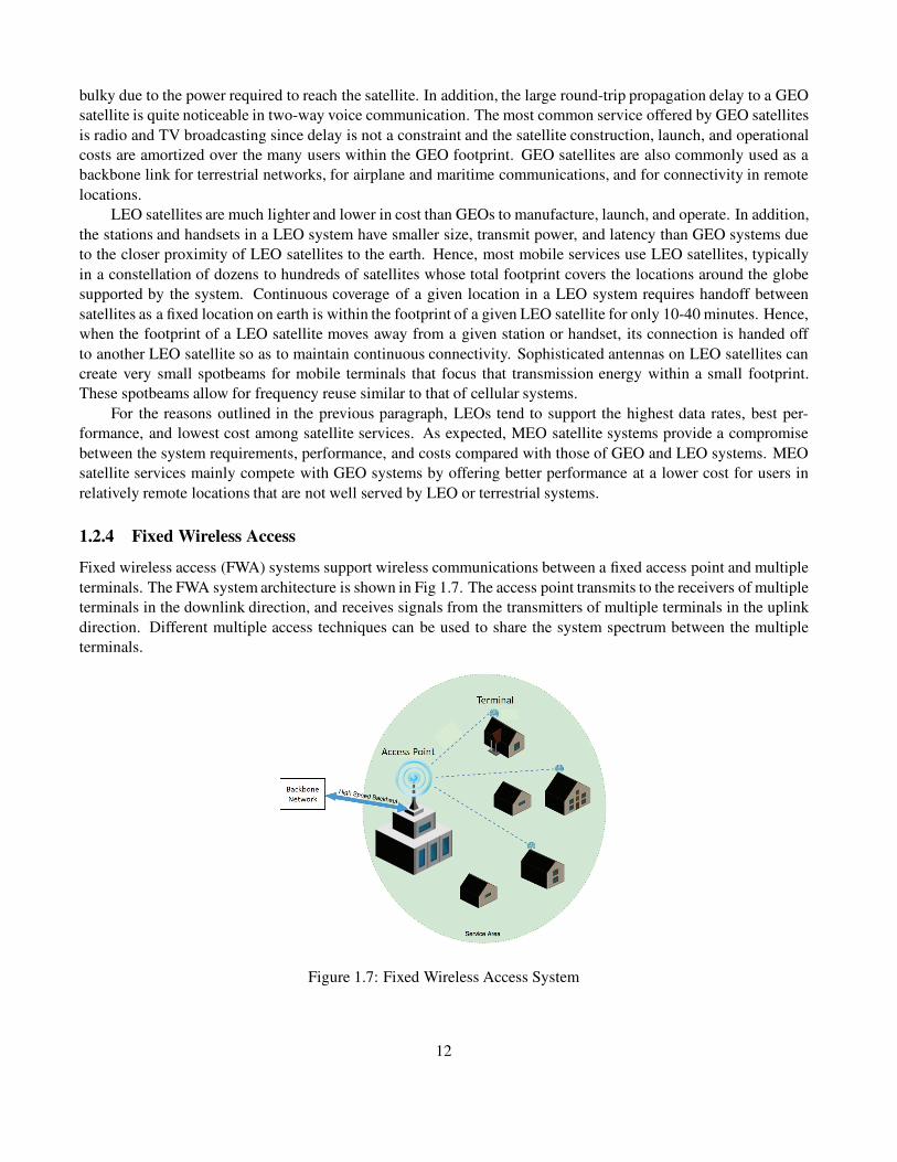
1.2.3 Satellite Systems

Satellite systems are another major component of the wireless communications infrastructure [14, 15]. There is a

plethora of satellite communications services available today, including mobile service to airplanes, ships, vehicles,

and hand-held terminals, fixed satellite service to earth stations, as well as broadcast radio and television service.

Fig. 1.6 illustrates the satellite architecture supporting all such services. One of the biggest advantages of satellites

over terrestrial wireless systems is their ability to provide coverage in remote areas.

Figure 1.6: Satellite System Architecture

Satellite communication systems consist of one or more satellites communicating with stations on earth or

in the air. Communication satellites typically serve as relays between stations on the ground and in some cases

provide direct links to other satellites as well. Ground stations may be at fixed locations, in which case their

antennas may be large to maximize received signal strength. Mobile stations and indoor fixed stations have smaller

antennas, typically on the order of 1-3 meters. The coverage area or footprint of a satellite depends on its orbit. A

GEO satellite can cover one or more continents, hence only a handful are needed to provide coverage for the entire

globe. However, the transmission latency between the earth and a GEO satellite is high, on the order of 300 ms.

MEO satellites have a coverage area of around ten thousand square kilometers and a latency of around 80 ms. A

LEO coverage area is about a thousand square kilometers with a latency of around 10 ms.

A GEO satellite provides continuous coverage to any station within its footprint, whereas a satellite with a

different orbit will have a fixed station within its footprint for only part of a 24 hour period. GEO satellites are

heavy, sophisticated, and costly to build and launch. Portable stations or handsets for GEOs tend to be large and

11

bulky due to the power required to reach the satellite. In addition, the large round-trip propagation delay to a GEO

satellite is quite noticeable in two-way voice communication. The most common service offered by GEO satellites

is radio and TV broadcasting since delay is not a constraint and the satellite construction, launch, and operational

costs are amortized over the many users within the GEO footprint. GEO satellites are also commonly used as a

backbone link for terrestrial networks, for airplane and maritime communications, and for connectivity in remote

locations.

LEO satellites are much lighter and lower in cost than GEOs to manufacture, launch, and operate. In addition,

the stations and handsets in a LEO system have smaller size, transmit power, and latency than GEO systems due

to the closer proximity of LEO satellites to the earth. Hence, most mobile services use LEO satellites, typically

in a constellation of dozens to hundreds of satellites whose total footprint covers the locations around the globe

supported by the system. Continuous coverage of a given location in a LEO system requires handoff between

satellites as a fixed location on earth is within the footprint of a given LEO satellite for only 10-40 minutes. Hence,

when the footprint of a LEO satellite moves away from a given station or handset, its connection is handed off

to another LEO satellite so as to maintain continuous connectivity. Sophisticated antennas on LEO satellites can

create very small spotbeams for mobile terminals that focus that transmission energy within a small footprint.

These spotbeams allow for frequency reuse similar to that of cellular systems.

For the reasons outlined in the previous paragraph, LEOs tend to support the highest data rates, best per-

formance, and lowest cost among satellite services. As expected, MEO satellite systems provide a compromise

between the system requirements, performance, and costs compared with those of GEO and LEO systems. MEO

satellite services mainly compete with GEO systems by offering better performance at a lower cost for users in

relatively remote locations that are not well served by LEO or terrestrial systems.

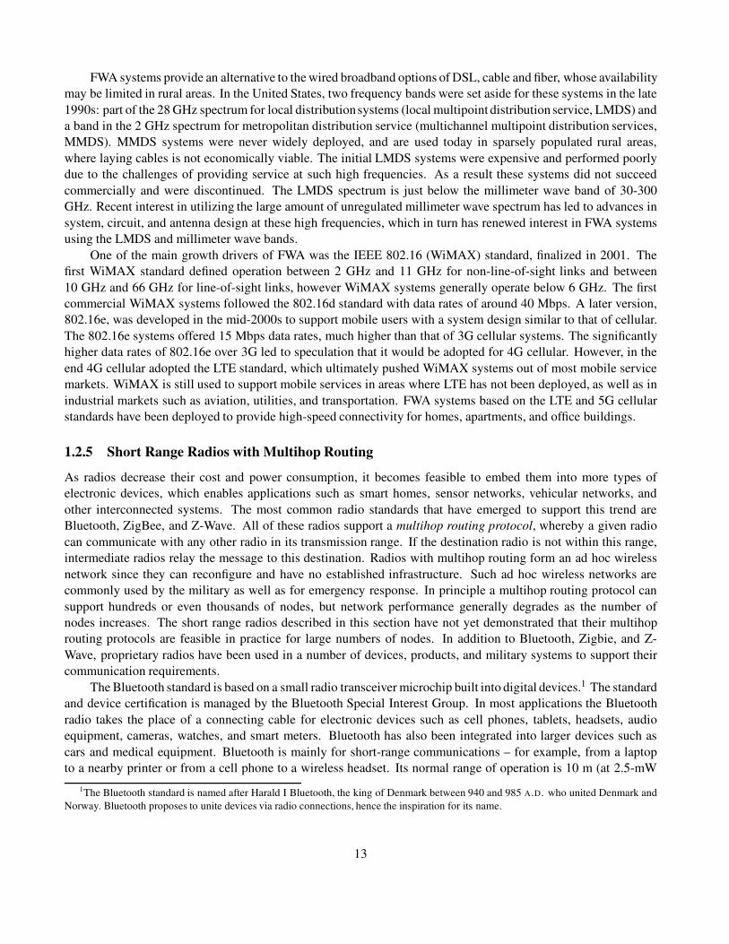
1.2.4 Fixed Wireless Access

Fixed wireless access (FWA) systems support wireless communications between a fixed access point and multiple

terminals. The FWA system architecture is shown in Fig 1.7. The access point transmits to the receivers of multiple

terminals in the downlink direction, and receives signals from the transmitters of multiple terminals in the uplink

direction. Different multiple access techniques can be used to share the system spectrum between the multiple

terminals.

Figure 1.7: Fixed Wireless Access System

12

FWA systems provide an alternative to the wired broadband options of DSL, cable and fiber, whose availability

may be limited in rural areas. In the United States, two frequency bands were set aside for these systems in the late

1990s: part of the 28 GHz spectrum for local distributionsystems (local multipoint distribution service, LMDS) and

a band in the 2 GHz spectrum for metropolitan distribution service (multichannel multipoint distribution services,

MMDS). MMDS systems were never widely deployed, and are used today in sparsely populated rural areas,

where laying cables is not economically viable. The initial LMDS systems were expensive and performed poorly

due to the challenges of providing service at such high frequencies. As a result these systems did not succeed

commercially and were discontinued. The LMDS spectrum is just below the millimeter wave band of 30-300

GHz. Recent interest in utilizing the large amount of unregulated millimeter wave spectrum has led to advances in

system, circuit, and antenna design at these high frequencies, which in turn has renewed interest in FWA systems

using the LMDS and millimeter wave bands.

One of the main growth drivers of FWA was the IEEE 802.16 (WiMAX) standard, finalized in 2001. The

first WiMAX standard defined operation between 2 GHz and 11 GHz for non-line-of-sight links and between

10 GHz and 66 GHz for line-of-sight links, however WiMAX systems generally operate below 6 GHz. The first

commercial WiMAX systems followed the 802.16d standard with data rates of around 40 Mbps. A later version,

802.16e, was developed in the mid-2000s to support mobile users with a system design similar to that of cellular.

The 802.16e systems offered 15 Mbps data rates, much higher than that of 3G cellular systems. The significantly

higher data rates of 802.16e over 3G led to speculation that it would be adopted for 4G cellular. However, in the

end 4G cellular adopted the LTE standard, which ultimately pushed WiMAX systems out of most mobile service

markets. WiMAX is still used to support mobile services in areas where LTE has not been deployed, as well as in

industrial markets such as aviation, utilities, and transportation. FWA systems based on the LTE and 5G cellular

standards have been deployed to provide high-speed connectivity for homes, apartments, and office buildings.

1.2.5 Short Range Radios with Multihop Routing

As radios decrease their cost and power consumption, it becomes feasible to embed them into more types of

electronic devices, which enables applications such as smart homes, sensor networks, vehicular networks, and

other interconnected systems. The most common radio standards that have emerged to support this trend are

Bluetooth, ZigBee, and Z-Wave. All of these radios support a multihop routing protocol, whereby a given radio

can communicate with any other radio in its transmission range. If the destination radio is not within this range,

intermediate radios relay the message to this destination. Radios with multihop routing form an ad hoc wireless

network since they can reconfigure and have no established infrastructure. Such ad hoc wireless networks are

commonly used by the military as well as for emergency response. In principle a multihop routing protocol can

support hundreds or even thousands of nodes, but network performance generally degrades as the number of

nodes increases. The short range radios described in this section have not yet demonstrated that their multihop

routing protocols are feasible in practice for large numbers of nodes. In addition to Bluetooth, Zigbie, and Z-

Wave, proprietary radios have been used in a number of devices, products, and military systems to support their

communication requirements.

The Bluetooth standard is based on a small radio transceiver microchip built into digital devices.1 The standard

and device certification is managed by the Bluetooth Special Interest Group. In most applications the Bluetooth

radio takes the place of a connecting cable for electronic devices such as cell phones, tablets, headsets, audio

equipment, cameras, watches, and smart meters. Bluetooth has also been integrated into larger devices such as

cars and medical equipment. Bluetooth is mainly for short-range communications – for example, from a laptop

to a nearby printer or from a cell phone to a wireless headset. Its normal range of operation is 10 m (at 2.5-mW

1The Bluetooth standard is named after Harald I Bluetooth, the king of Denmark between 940 and 985 A.D. who united Denmark and

Norway. Bluetooth proposes to unite devices via radio connections, hence the inspiration for its name.

13

transmit power), and this range can be increased to 100 m by increasing the transmit power to 100 mW. The system

operates in the unlicensed 2.4-GHz frequency band, so it can be used worldwide without any licensing issues. The

Bluetooth standard provides one data channel at 723.2 kbps. In this mode, there is a reverse channel with a data

rate of 57.6 kbps. The specification also allows up to three additional channels each at a rate of 64 kbps, which

are primarily used for voice connections with headsets. These different modes result in an aggregate bit rate of

approximately 1 Mbps. An enhanced data rate mode provides up to 3 Mbps, while a low-energy mode significantly

reduces power consumption at the expense of range or data rate.

Bluetooth uses frequency hopping for multiple access with a carrier spacing of 1 MHz. Typically, up to eighty

different frequencies are used for a total bandwidth of 80 MHz. At any given time, the bandwidth available is

1 MHz. Bluetooth radios form small ad hoc networks of up to eight devices sharing the same logical channel (same

hop sequence), which is called a piconet. Different channels (different hopping sequences) can simultaneously

share the same 80 MHz bandwidth. Collisions will occur when devices in different piconets that are on different

logical channels happen to use the same hop frequency at the same time. As the number of piconets in an area

increases, the number of collisions increases and performance degrades. The original Bluetooth standard was

developed jointly by 3 Com, Ericsson, Intel, IBM, Lucent, Microsoft, Motorola, Nokia, and Toshiba. Many

additional manufactures have contributed to each new generation of the standard. Bluetooth is integrated into a

wide range of electronic devices with several billion Bluetooth-enabled devices shipped annually.

The ZigBee2 radio specification is designed for lower cost and power consumption than Bluetooth. It follows

the IEEE 802.15.4 standard with device certification managed by the Zigbie Alliance. The radio operates in the

same 2.4 GHz ISM band as Bluetooth. Zigbee radios support data rates of up to 250 kbps at a range of up to 30 m.

These data rates are slower than Bluetooth, but in exchange the radio consumes significantly less power with a

larger transmission range. Zigbee also operates in a “green” mode whereby the radio is powered through energy

harvesting of its environment, reducing or in some cases completely elimiating the need for battery power. The

goal of ZigBee is to provide radio operation for months or years without recharging, thereby targeting devices such

as smart tags, meters, lights, and thermostats, as well as those used for sensing and automation.

Z-Wave radios are designed primarily for smart home applications with operation in the 900 MHz ISM band.

Since power falls off more slowly in this band than at the higher 2.4 GHz spectrum, Z-Wave radios have a higher

range than standard Zigbee or Bluetooth radios, on the order of 100 m. In addition, there is no interference between

Z-Wave radios and those operating in the crowded 2.4 GHz band, including Wi-Fi as well as Bluetooth and Zigbee.

On the downside, Z-Wave has significantly lower data rates than either Bluetooth or Zigbee, ranging from 10 to

100 Kbps. The Z-Wave standard and device certification is managed by the Z-Wave Alliance.

1.3 Wireless Spectrum

1.3.1 Regulation

Most countries have government agencies responsible for allocating and controlling use of the radio spectrum.

In the United States, spectrum is allocated by the Federal Communications Commission (FCC) for commercial

use and by the Office of Spectral Management (OSM) under the auspices of the National Telecommunications

and Information Administration (NTIA) for government use. Countries throughout the world have similar regula-

tory agencies to regulate spectrum within their borders. Certain regions of the world have a common regulatory

agency for spectrum allocation, e.g. commercial spectral allocation across Europe is governed by the European

Telecommunications Standards Institute (ETSI). Satellite systems cover large areas spanning many countries and

sometimes the globe. Globally, spectrum is allocated by the International Telecommunications Union Radio Com-

2ZigBee takes its name from the dance that honey bees use to communicate information about newly found food sources to other

members of the colony.

14

munications group (ITU-R) through its World Radiocommunication Conferences (WRC). The standards arm of

this body, ITU-T, adopts telecommunication standards for global systems that must interoperate across national

boundaries. Regulatory agencies typically have many competing considerations in deciding how to allocate any

given block of spectrum, including whether to allocate it for commercial, military, or shared use. These deci-

sions are generally driven by a broad mandate to regulate spectrum “in the public interest,” as stated in the U.S.

Communications Act of 1934 establishing the FCC.

Historically government agencies allocated spectral blocks for specific uses and assigned licenses to use these

blocks to specific groups or companies. For example, in the 1980s the FCC allocated spectrum around 850 MHz

for analog cellular phone service, in particular 824-849 MHz for the downlink (base station to mobile) and 869-894

MHz in the uplink (mobile to base station). Spectral licenses were provided to two operators in each geographical

area based on a number of criteria. While this method of licensed spectral allocation is still used in some circum-

stances, a fundamental shift occurred worldwide in the early 1990s for licensed spectrum to be auctioned to the

highest bidder, with some restrictions in place to ensure fairness and competitive use of the spectrum. The basis for

the shift was the market-based reasoning that auctions provide the fairest and most efficient way for governments

to allocate the limited spectral resource and, moreover, this method provides significant revenue to the government.

However, auctions are not universally supported for spectral allocation based on the contention that they can stifle

innovation, limit competition, and hurt technology adoption. Specifically, the high cost of spectrum dictates that

only large companies or conglomerates can purchase it. Moreover, the large investment required to obtain spectrum

can delay, sometimes indefinitely, the ability to invest in infrastructure for system rollout. Finally, high spectral

cost is usually passed on to the end user. The early 3G spectral auctions, with suspected collusion between bidders,

low bids, and several auction winners that ultimately defaulted, provided ammunition to the opponents of spectral

auctions. Lessons learned from these early auctions were adopted in the design of subsequent auctions, which

generally went smoothly and raised up to tens of billions of dollars. In addition, reverse or incentive auctions were

initiated starting in 2016, whereby license holders could sell back their spectrum to regulatory bodies for future

auctioning. A comprehensive treatment of spectrum regulation and its allocation through auctions can be found in

[16].

In addition to spectral auctions, spectrum can be set aside in specific frequency bands, called unlicensed

bands, that are free to use without a license according to a specific set of rules. The rules may correspond to a spe-

cific access protocol to ensure fairness, restrictions on power levels, and so forth. The purpose of these unlicensed

bands is to encourage innovation and low-cost implementation. Wi-Fi is often associated with the unlicensed fre-

quency bands, however it is just one of the hundreds of successful unlicensed systems, which include standardized

short-range radio systems as well as proprietary radios in cordless phones, wireless home security systems, baby

monitors, medical equipment, inventory systems, smart meters, and keyless automobile entry systems. Indeed, it is

estimated that unlicensed wireless devices contribute tens of billions of dollars annually to the US economy alone.

A major difficulty of unlicensed bands is that they can be killed by their own success. If many unlicensed devices

on the same channel are used in close proximity then they interfere with each other, which can make the band

unusable. Cellular systems can also operate in the unlicensed bands by following the unlicensed spectrum rules.

However, since these systems can used their licensed bands for control, they have an advantage over systems such

as Wi-Fi that use the unlicensed bands for both control and data transmission and can crowd out Wi-Fi users as

a result [17]. Much of the spectrum above 30 GHz is unregulated or lightly regulated, and hence can be used by

unlicensed users with little to no restriction.

Underlay systems are another alternative for allocating spectrum. An underlay system operates as a secondary

user in a licensed frequency band simultaneous with the licensed users in a manner such that the licensed users

experience minimal interference from them. This is usually accomplished by spreading the signal over a very

wide bandwidth, typically more than 500 MHz, and restricting its power per Hertz. The first underlay standard

approved for operation was ultrawideband (UWB) communications [18]. Specifically, in 2002 the FCC approved

15

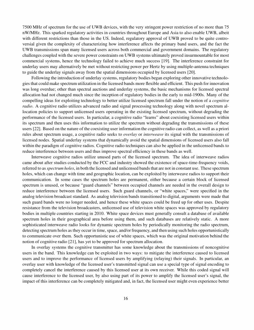
7500 MHz of spectrum for the use of UWB devices, with the very stringent power restriction of no more than 75

nW/MHz. This sparked regulatory activities in countries throughout Europe and Asia to also enable UWB, albeit

with different restrictions than those in the US. Indeed, regulatory approval of UWB proved to be quite contro-

versial given the complexity of characterizing how interference affects the primary band users, and the fact the

UWB transmissions span many licensed users across both commercial and government domains. The regulatory

challenges coupled with the severe power constraints on UWB systems ultimately proved insurmountable for most

commercial systems, hence the technology failed to achieve much success [19]. The interference constraint for

underlay users may alternatively be met without restricting power per Hertz by using multiple-antenna techniques

to guide the underlay signals away from the spatial dimensions occupied by licensed users [20].

Following the introduction of underlay systems, regulatory bodies began exploring other innovative technolo-

gies that could make spectrum utilization in the licensed bands more flexible and efficient. This push for innovation

was long overdue; other than spectral auctions and underlay systems, the basic mechanisms for licensed spectral

allocation had not changed much since the inception of regulatory bodies in the early to mid-1900s. Many of the

compelling ideas for exploiting technology to better utilize licensed spectrum fall under the notion of a cognitive

radio. A cognitive radio utilizes advanced radio and signal processing technology along with novel spectrum al-

location policies to support unlicensed users operating in the existing licensed spectrum, without degrading the

performance of the licensed users. In particular, a cognitive radio “learns” about coexisting licensed users within

its spectrum and then uses this information to utilize the spectrum without degrading the transmissions of these

users [22]. Based on the nature of the coexisting user information the cognitive radio can collect, as well as a priori

rules about spectrum usage, a cognitive radio seeks to overlay or interweave its signal with the transmissions of

licensed nodes. Spatial underlay systems that dynamically avoid the spatial dimensions of licensed users also fall

within the paradigm of cognitive radios. Cognitive radio techniques can also be applied in the unlicensed bands to

reduce interference between users and thus improve spectral efficiency in these bands as well.

Interweave cognitive radios utilize unused parts of the licensed spectrum. The idea of interweave radios

came about after studies conducted by the FCC and industry showed the existence of space-time-frequency voids,

referred to as spectrum holes, in both the licensed and unlicensed bands that are not in constant use. These spectrum

holes, which can change with time and geographic location, can be exploited by interweave radios to support their

communication. In some cases the spectrum holes are permanent, either because a certain block of licensed

spectrum is unused, or because “guard channels” between occupied channels are needed in the overall design to

reduce interference between the licensed users. Such guard channels, or “white spaces,” were specified in the

analog television broadcast standard. As analog television bands transitioned to digital, arguments were made that

such guard bands were no longer needed, and hence these white spaces could be freed up for other uses. Despite

resistance from the television broadcasters, unlicensed use of television white spaces was approved by regulatory

bodies in multiple countries starting in 2010. White space devices must generally consult a database of available

spectrum holes in their geographical area before using them, and such databases are relatively static. A more

sophisticated interweave radio looks for dynamic spectrum holes by periodically monitoring the radio spectrum,

detecting spectrum holes as they occur in time, space, and/or frequency, and then using such holes opportunistically

to communicate over them. Such opportunistic use of white spaces, which was the original motivation behind the

notion of cognitive radio [21], has yet to be approved for spectrum allocation.

In overlay systems the cognitive transmitter has some knowledge about the transmissions of noncognitive

users in the band. This knowledge can be exploited in two ways: to mitigate the interference caused to licensed

users and to improve the performance of licensed users by amplifying (relaying) their signals. In particular, an

overlay user with knowledge of the licensed user’s transmitted signal can use a special type of signal encoding to

completely cancel the interference caused by this licensed user at its own receiver. While this coded signal will

cause interference to the licensed user, by also using part of its power to amplify the licensed user’s signal, the

impact of this interference can be completely mitigated and, in fact, the licensed user might even experience better

16

performance than without the existence of the overlay user. The overlay cognitive radio paradigm was originally

proposed in [23] and capacity limits as well as practical implementations of overlay systems have been extensively

studied since then. However, regulatory agencies have not yet considered allowing overlay systems to operate in

the licensed spectrum.

Overlay, underlay, and interweave radio innovations could make spectrum utilization far more efficient than it

is today, in both the licensed and unlicensed bands, thereby enabling new wireless systems, products, and applica-

tions. More details on the technologies behind these cognitive radio paradigms will be discussed in Chapter 16.7.

However, even once these and other cognitive radio technologies are fully developed, changing regulatory policies

to include these novel mechanisms will likely be fraught with conflicting opinions from government, industry, and

the end users about what best serves the public interest in the allocation of spectrum.

1.3.2 Properties and Existing Allocations

Most wireless communication systems operate in the radio spectrum between 30 MHz and 30 GHz, with some

in the millimeter wave frequency band (30 GHz-300 GHz) as well. For communication systems at frequencies

below 800 MHz, antenna sizes are too large for small devices, and at frequencies above 3 GHz, signal attenuation

with distance precludes long-range transmission. Given these tradeoffs, the primary frequency bands that fueled

the extraordinary grown of cellular, Wi-Fi, and short-range radios like Bluetooth were in the 0.8-3 GHz range.

As those frequency bands became congested, these systems moved to adjacent bands (0.6-0.8 for cellular and 3-5

GHz for cellular and Wi-Fi). Cellular and Wi-Fi systems started to expand into the millimeter wave bands as well

due to the plentiful spectrum there. A similar evolution into higher frequency bands occured in satellite systems.

In particular, early satellite systems used the 4-8 GHz C band, but over time moved into the X (8-12.5 GHz), Ku

(12-18 GHz), K (18-26 GHz) and Ka (26-40 GHz) bands. The K bands were assigned to terrestrial fixed wireless

services as well, including LMDS. Note that the required antenna size for good reception is inversely proportional

to the signal frequency, so moving systems to a higher frequency allows for more compact antennas. However,

received signal power with nondirectional antennas is proportional to the inverse of frequency squared, so it is

harder to cover large distances with high-frequency signals.

As discussed previously, spectrum is allocated either in licensed bands (which regulatory bodies assign to

specific operators) or in unlicensed bands (which can be used by any system subject to certain operational re-

quirements). Often different countries try to match their frequency bands for licensed and unlicensed use so that

technology developed for that spectrum is compatible worldwide, however that isn’t possible if a country has al-

located one of these frequency bands to another use. Figure 1.8 shows the unlicensed spectrum allocations in

the United States. In most cases there are similar frequency allocations in Europe and Asia. ISM Band I at 900

MHz has limited spectrum availability as well as licensed users transmitting at high power who interfere with the

unlicensed users. Since performance in this band is somewhat poor, it is not heavily utilized by unlicensed devices.

The U-NII bands have a total of 555 MHz of spectrum in four separate bands, with different power restrictions.

In addition, some countries have imposed restrictions on parts of the U-NII bands so that unlicensed systems must

avoid interference with radar systems licensed to operate in those bands.

Figure 1.9 shows the frequency bands allocated to current and legacy cellular systems in the United States

along with their band name abbreviations3. Note from this table that 4G (LTE) systems operate in the 3.5 GHz

CBRS band and the 5.2 GHz U-NII band, which are unlicensed bands, and hence must be shared with other

unlicensed users. Prior to 4G, cellular systems operated only in dedicated licensed spectrum and hence interference

was centrally managed. Under this new paradigm of spectrum sharing, the licensed and unlicensed users using the

same band must manage shared access and interference between the different systems.

3Band abbreviations are Specialized Mobile Radio (SMR); Personal Communication System (PCS); Advanced Wireless Services

(AWS); Digital Dividend (DD); Wireless Communications Services (WCS); Broadband Radio Service (BRS); Citizen’s Broadband Ra-

17

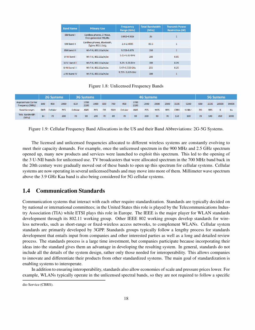
Figure 1.8: Unlicensed Frequency Bands

Figure 1.9: Cellular Frequency Band Allocations in the US and their Band Abbreviations: 2G-5G Systems.

The licensed and unlicensed frequencies allocated to different wireless systems are constantly evolving to

meet their capacity demands. For example, once the unlicensed spectrum in the 900 MHz and 2.5 GHz spectrum

opened up, many new products and services were launched to exploit this spectrum. This led to the opening of

the 3 U-NII bands for unlicensed use. TV broadcasters that were allocated spectrum in the 700 MHz band back in

the 20th century were gradually moved out of these bands to open up this spectrum for cellular systems. Cellular

systems are now operating in several unlicensed bands and may move into more of them. Millimeter wave spectrum

above the 3.9 GHz Kaa band is also being considered for 5G cellular systems.

1.4 Communication Standards

Communication systems that interact with each other require standardization. Standards are typically decided on

by national or international committees; in the United States this role is played by the Telecommunications Indus-

try Association (TIA) while ETSI plays this role in Europe. The IEEE is the major player for WLAN standards

development through its 802.11 working group. Other IEEE 802 working groups develop standards for wire-

less networks, such as short-range or fixed-wireless access networks, to complement WLANs. Cellular system

standards are primarily developed by 3GPP. Standards groups typically follow a lengthy process for standards

development that entails input from companies and other interested parties as well as a long and detailed review

process. The standards process is a large time investment, but companies participate because incorporating their

ideas into the standard gives them an advantage in developing the resulting system. In general, standards do not

include all the details of the system design, rather only those needed for interoperability. This allows companies

to innovate and differentiate their products from other standardized systems. The main goal of standardization is

enabling systems to interoperate.

In addition to ensuring interoperability, standards also allow economies of scale and pressure prices lower. For

example, WLANs typically operate in the unlicensed spectral bands, so they are not required to follow a specific

dio Service (CBRS).

18

standard. The first generation of WLANs were not standardized and so specialized components were needed for

many systems, leading to excessively high cost that, when coupled with poor performance, led to limited adoption.

This experience resulted in a strong push to standardize the next WLAN generation, which yielded the highly

successful IEEE 802.11 family of standards. Adherence of products to the 802.11 standard is certified by the

Wi-Fi Alliance.

There are, of course, disadvantages to standardization. The standards process is not perfect, as company

participants often have their own agendas, which do not always coincide with the best technology or the best

interests of consumers. In addition, the standards process must be completed at some point, after which it becomes

more difficult to add new innovations and improvements to an existing standard. Finally, the standards process

can become quite politicized. This happened in Europe with 1st generation cellular systems, where each country

had its own standard, and with the second generation of cellular phones in the United States which ultimately

adopted three different standards. The formation of the 3GPP standards body to create a single unified cellular

standard throughout much of the world was a response to these pitfalls in earlier cellular standards, and is largely

responsible for the massive growth in and success of cellular technology. Hence, despite its flaws, standardization

is often an essential component of wireless system design and operation in order to ensure its success.

1.5 Wireless Vision

“It is always wise to look ahead, but difficult to look further than you can see.” - Winston Churchill

Wireless communication is ubiquitious in the world we live in, enabling vast connectivity among people and

devices as well as rapid access to information. Wireless technology impacts every aspect of modern life: culture,

business, politics, economics, health, entertainment, and education. So what might the future bring?

Demand for higher data rates seems unending, hence future wireless systems could support peak speeds of

hundreds or perhaps thousands of Gigabits per second. There are billions of people and locations throughout the

world today without wireless (or wired) connectivity, so perhaps future systems will fill in these coverage holes

so that no person or place on the planet lacks wireless connectivity. Wireless devices might shrink to such small

sizes that they can be deployed within any object or living being. Some wireless devices may be powered from a

very small battery or even self-power through energy harvesting or wireless charging, eliminating the need to ever

plug in. Wireless technology might evolve to support the “five-nines” standard in reliability for tradition telephone

service, meaning that the service is reliable 99.999% of the time in any location, indoors and out. Finally, wireless

systems must be extremely secure against natural impairments as well as eavesdroppers, attackers and spoofers.

If this vision of wireless technology comes to pass, what will it enable? In addition to providing people

with voice, high-speed data, and broadcast entertainment, future wireless networks will also support machine-to-

machine communications for tens of billions of devices. In the home these networks will enable a new class of

intelligent electronic devices that can interact with each other and with the Internet. Such “smart” homes will

drastically improve energy efficiency, security, emergency response, as well as help the elderly and disabled with

assisted living. Other applications of these networks include sensing and data collection in the power grid to

improve robustness and efficiency, “smart cities” that provide services such as trash collection and road mainte-

nance when the need is detected, and in-body communications for medical devices, biosensors, and targeted drug

delivery. Wireless video and virtual reality will permeate the home and any place that people congregate with

entertainment, and also enable remote classrooms, remote training facilities, and remote hospitals anywhere in

the world. Wireless sensor networks will improve monitoring of and response to fire hazards, toxic waste sites,

stress and strain in buildings and bridges, carbon dioxide movement, and the spread of chemicals and gases at

disaster sites. Finally, wireless networks with very low latency will enable distributed control systems with remote

19

devices, sensors, and actuators linked together via wireless communication channels. Such systems will in turn en-

able intelligent transportation systems including self-driving vehicles, mobile robots and drones, as well as easily

reconfigurable industrial automation.

The exponential growth of smartphone use and wireless Internet access has led to great optimism about

wireless technology in general. Obviously not all wireless applications will flourish. While many wireless systems

and companies have enjoyed spectacular success, there have also been many failures along the way, including

the first generation of wireless LANs and LEO satellite systems, as well as wide area data services, and fixed

wireless access to the home. Indeed, it is impossible to predict what wireless failures and triumphs lie on the

horizon. Moreover, there must be sufficient flexibility and creativity among both engineers and regulators to allow

for accidental successes. It is clear, however, that the current and emerging wireless systems of today – coupled

with the vision of applications that wireless can enable – ensure a bright future for wireless technology.

1.6 Technical Challenges

This section provides an overview of the many technical challenges that must be addressed to make the wireless

vision a reality. These challenges extend across all aspects of the system, including hardware design, channel

characterization, physical layer and multiple access techniques as well as networking protocols and architectures.

Techniques to address many of these challenges are described in subsequent chapters of the book.

The design of wireless systems begins with a model for the underlying channel through which the signals will

propagate. In all such channels, signal power decreases with distance due to the physics of propagation as well as

attenuation from blocking objects. These signal propagation models are developed in Chapter 2. If the transmitter,

receiver, or surrounding objects are moving, the channel changes randomly with time due to changing reflections

and attenuation. These random channel variations, whose statistical models are developed in Chapter 3, make it

difficult to design reliable systems with guaranteed performance. Channel characteristics, including signal attenu-

ation, also depend on the frequency of operation. In particular, received power generally decreases with the carrier

frequency and, in the case of free space propagation with omnidirectional antennas, it is inversely proportional

to the square of this frequency. Thus, most wireless systems today operate at carrier frequencies below 5 GHz

to ensure good coverage, leading to a spectrum shortage in this range of frequencies. Moving to higher carrier

frequencies, such as millimeter wave (30-300 GHz) or terahertz (.3-3 THz), provides much more spectrum than

what is available in the lower frequency bands. However, these higher frequencies of operation reduce range unless

energy is directionally focused using multiple or directional antenna techniques. Signal propagation characteristics

at these frequencies create challenges in designing reliable communication links, as described in Chapter 2.9.5. In

addition, hardware components are expensive and power hungry.

The maximum data rate that can be reliably sent over a wireless (or wireline) channel is its Shannon capacity,

which is derived in Chapter 4. This capacity is directly proportional to the channel bandwidth, i.e. the amount of

spectrum allocated to the channel. This rate also depends on the number of antennas at the transmitter and receiver,

as multiple-input multiple-output (MIMO) techniques allow for independent data streams to be transmitted along

the independent spatial dimensions these multiple antennas create, as described in Chapter 10. Achievable data

rates for a given wireless system also depend on signal propagation and interference characteristics. Due to these

challenges, data rates for both cellular and Wi-Fi systems are several orders of magnitude lower than for a fiber

optic cable, but that could change as millimeter wave systems are deployed.

In terms of hardware challenges, as the size of wireless devices shrink, breakthroughs are needed to make

both the analog and digital circuitry significantly smaller, cheaper, and more energy efficient. Wireless systems

operating at millimeter wave and higher frequencies require cheap and reliable RF components, which remains a

significant challenge. The size, power consumption, and precision of analog-to-digital converters is also becoming

a bottleneck as systems move to larger bandwidths. Finally, large antenna arrays that improve signal propagation

20

and mitigate interference require hardware innovations, including hybrid analog and digital processing, to reduce

their footprint, power consumption, and cost.

The physical layer design of wireless systems today is quite sophisticated, with dense-constellation modula-

tion (Chapters 5-6), diversity and adaptive modulation techniques to combat random signal variations (Chapters

7 and 9), powerful error-correction coding (Chapter 8), as well as techniques to combat intersymbol interference

caused by delayed signal components that arise from channel reflections (Chapters 11-13). Systems operating in

rapidly changing environments require new modulation, coding, detection, and multi-antenna techniques that are

robust to such changes when adaptation to them is infeasible. Machine learning may play a role in improving

physical layer techniques for channel estimation, signal detection, decoding, and equalizaiton, particularly when

channels are hard to model, hard to estimate, or rapidly varying [24, 25]. In addition, algorithms that best exploit

the many spatial degrees of freedom offered by large antenna arrays are needed. For energy-constrained systems,

particularly those running off non-rechargeable batteries, communication schemes must be developed that can meet

performance requirements while minimizing total system power consumption (for signal transmission, reception,

and processing).

Multiple access techniques, developed in Chapter 14, allow users to share the same system bandwidth. This

bandwidth sharing is done either through coordinated access, as in cellular systems and current Wi-Fi standards,

or through distributed techniques, as used in early generations of Wi-Fi systems. Most wireless systems use access

schemes that assign orthogonal time and frequency slices of the total system bandwidth to different users. For

MIMO systems, independent spatial dimensions can be used as separate channels as well. Non-orthogonal access

designs improve spectral efficiency by overlapping channels in the time, frequency, code, or spatial dimensions

while managing the interference that results. Channel assignment is done by the base stations in cellular systems

and by access points in Wi-Fi systems. Wireless access techniques are ripe for innovation, in the centralized and

distributed mechanisms used to assign channels as well as in slicing up channels in a non-orthogonal manner to

increases spectral efficiency with minimal interference. Machine learning is also being applied to multiple access,

resource allocation, and scheduling [24].

The network architectures and protocols for future wireless systems must support a much wider range of

devices and applications than exist today. For infrastructure-based systems like cellular networks (Chapter 15),

this will require a more flexible architecture, with a range of cell sizes, greater densification of cells, as well as

significant data processing, dynamic optimization, and resource allocation that may be centralized, decentralized,

or centralized within a subsets of nodes (coined neighborhood or “fog-based” optimization). Rethinking cellular

system architectures to take into account novel forms of cooperation across base stations and users to exploit rather

than mitigate interference may lead to significantly higher capacity and robustness. Reduction of latency and over-

head for applications with short delay-constrained messages is also needed, as are innovations in energy-efficient

architectures, e.g. for systems whose backbone is powered by batteries, solar, other forms of energy harvesting, or

wireless power transfer. In ad hoc wireless networks (Chapter 16), advances in cooperative techniques for trans-

mission, reception, and relaying have the potential to significantly improve coverage, reliability, and data rates.

Seamless handoff between different wireless networks, such as Wi-Fi and cellular, is precluded by existing

protocols and addressing mechanisms, which must evolve to allow a device to continuously connect on any and all

available networks. How best to utilize a multiplicity of available networks for a given device or application is an

open challenge. Many wireless systems consist of predominantly wired links, with wireless as the last hop only.

Hence, challenges in wired networking, such as latency and bandwidth shortages, impact wireless networks as

well. Deployment of caching and computation capabilities in base stations and Wi-Fi access points give rise to new

design challenges; should applications utilize these edge capabilities or rely on more powerful capabilities situated

farther from the network edge, which entail more latency to access. Security is also more difficult to implement for

signals traveling over wireless channels, since the airwaves are susceptible to snooping and jamming by anyone

with an RF antenna.

21

Chapter 1 Problems

1. As storage capability increases, we can store larger and larger amounts of data on smaller and smaller

storage devices. Indeed, we can envision microscopic computer chips storing terraflops of data. Suppose

this data is to be transfered over some distance. Discuss the pros and cons of putting a large number of these

storage devices in a truck or drone and driving or flying them to their destination rather than sending the data

electronically.

2. Describe two technical advantages and disadvantages of wireless systems that use bursty data transmission

rather than continuous data transmission.

3. Fiber optic cable typically exhibits a probability of bit error of Pb = 10−12. A form of wireless modulation,

DPSK, has Pb = 1/2γ in some wireless channels, where γ is the average SNR. Find the average SNR

required to achieve the same Pb in the wireless channel as in the fiber optic cable. Because of this extremely

high required SNR, wireless channels typically have Pb much larger than 10−12.

4. Find the round-trip delay of data sent between a satellite and the earth for LEO, MEO, and GEO satellites

assuming the speed of light is 3 · 108 m/s. If the maximum acceptable delay for a voice system is 30 ms,

which of these satellite systems would be acceptable for two-way voice communication?

5. What applications might significantly increase the demand for wireless data?

6. This problem illustrates some of the economic issues facing service providers for mixed-media systems.

Suppose you are a service provider with 120 kHz of bandwidth that you must allocate between voice and

data users. The voice users require 20 kHz of bandwidth and the data users require 60 kHz of bandwidth. So,

for example, you could allocate all of your bandwidth to voice users, resulting in six voice channels, or you

could divide the bandwidth into one data channel and three voice channels, etc. Suppose further that this is a

time-division system with timeslots of duration T . All voice and data call requests come in at the beginning

of a timeslot, and both types of calls last T seconds. There are six independent voice users in the system:

each of these users requests a voice channel with probability .2 and pays $.20 if his call is processed. There

are two independent data users in the system: each of these users requests a data channel with probability .5

and pays $.50 if his call is processed. How should you allocate your bandwidth to maximize your expected

revenue?

7. Describe three disadvantages of using a fixed wireless access systems instead of DSL or cable. Describe

three scenarios where the disadvantages override the advantages.

8. Cellular systems have migrated to Hetnets consisting of a mix of macrocells and small cells in order to

increase system capacity and energy efficiency. Name at least three design issues that are complicated by

this trend.

9. Why does minimizing the reuse distance maximize the spectral efficiency of a cellular system?

10. This problem demonstrates the capacity increase associated with a decrease in cell size. Consider a square

city of 100 square kilometers. Suppose you design a cellular system for this city with square cells, where

every cell (regardless of cell size) has 100 channels and so can support 100 active users. (In practice, the

number of users that can be supported per cell is mostly independent of cell size as long as the propagation

model and power scale appropriately.)

(a) What is the total number of active users that your system can support for a cell size of 1 km2?

22

(b) What cell size would you use if your system had to support 250,000 active users?

Now we consider some financial implications based on the fact that users do not talk continuously. Assume

that Friday from 5–6 P.M. is the busiest hour for cell-phone users. During this time, the average user places a

single call, and this call lasts two minutes. Your system should be designed so that subscribers need tolerate

no greater than a 2% blocking probability during this peak hour. (Blocking probability is computed using

the Erlang B model: Pb = (AC/C!)/(∑c

k=0 Ak/k!

)

, where C is the number of channels and A = UµHfor U the number of users, µ the average number of call requests per unit time per user, and H the average

duration of a call [5, Chap. 3.6].

(c) How many total subscribers can be supported in the macrocell system

(1-km2 cells) and in the microcell system (with cell size from part (b))?

(d) If a base station costs $500,000, what are the base station costs for each system?

(e) If the monthly user fee in each system is $50, what will be the monthly revenue in each case? How long

will it take to recoup the infrastructure (base station) cost for each system?

23

Bibliography

[1] G.R.M. Garratt, The Early History of Radio: From Faraday to Marconi, IEEE History of Technology Series,

1994.

[2] S. M. Cherry, “What went wrong at Ricochet?,” IEEE Spectrum, Vol. 39, No. 3, pp. 60-61, March 2002.

[3] The Innovation Journey of Wi-Fi: The Road to Global Success, Edited by W. Lemstra, V. Hayes and J.

Groenewegen, Cambridge University Press, 2011.

[4] D. H. Ring, “Mobile Telephony - Wide Area Coverage,” Bell System Tech. Memo, Dec. 1947.

[5] ”High Capacity Mobile Telephone System Feasibility Studies and System Plan” J. Engel, R. Frenkiel, and P.

Porter, FCC Proposal, 1971.

[6] V.H. McDonald, “The Cellular Concept,” Bell System Tech. J, pp. 15-49, Jan. 1979.

[7] P. Nelson, “A new breed of broadband satellites could have you living on a desert island”, Network World,

July 2014.

[8] F. Abrishamkar and Z. Siveski, “PCS global mobile satellites,” IEEE Commun. Mag.,, pp. 132-136, Sep.

1996.

[9] M. Sauter From GSM to LTE-Advanced Pro and 5G: An Introduction to Mobile Networks and Mobile Broad-

band, 3rd ed., Wiley, 2017.

[10] E. Dahlman, S. Parkvall, and J. Skold, 5G NR: The Next Generation Wireless Access Technology, Academic

Press, 2018.

[11] E. Perahia and R. Stacey, Next Generation Wireless LANs: 802.11n and 802.11ac, 2nd ed., Cambridge

University Press, 2013.

[12] C. Wang, T. Jiang, and Q Zhang, ZigBee Network Protocols and Applications, CRC Press, 2014.

[13] K. Townsend, C. Cufi, Akiba, and R. Davidson, Getting Started with Bluetooth Low Energy: Tools and

Techniques for Low-Power Networking, O’Reilly Media, 2014.

[14] J. Pelton, S. Madry, and S. Camacho-Lara (eds), Handbook of Satellite Applications. Springer, Cham, 2017.

[15] S. K. Sharma, S. Chatzinotas, and P.-D. Arapoglou (eds.), Satellite Communications in the 5G Era Year, IET

Telecommunication Series, 2018

[16] M. Cave and W. Webb, Spectrum Management - Using the Airwaves for Maximum Social and Economic

Benefit, Cambridge University Press, 2016.

24

[17] F. M. Abinader et al., ”Enabling the coexistence of LTE and Wi-Fi in unlicensed bands,” IEEE Commun.

Mag., vol. 52, no. 11, pp. 54-61, Nov. 2014.

[18] S. Emami, UWB Communication Systems: Conventional and 60 GHz: Principles, Design and Standards,

Springer, 2013.

[19] L. Frenzel, “What ever happened to ultrawideband wireless,” Electronic Design, Sep. 2014.

[20] R. Zhang and Y. C. Liang, Exploiting multi-antennas for opportunistic spectrum sharing in cognitive radio

networks, IEEE J. Sel. Topics Signal Proc., vol. 2, no. 1, pp. 88-102, Feb. 2008.

[21] J. Mitola and G. Q. Maguire, ”Cognitive radio: making software radios more personal,” IEEE Personal

Commun., Vol. 6, No. 4, pp. 13-18, Aug. 1999.

[22] E. Biglieri, A. J. Goldsmith, L. J. Greenstein, N. B. Mandayam, and H. V. Poor, Principles of Cognitive

Radio, Cambridge University Press, 2012.

[23] N. Devroye, P. Mitran, and V. Tarokh, Achievable Rates in Cognitive Radio Channels, Proc. 39th Annual

Conf. Info. Sci. and Sys., Mar. 2005.

[24] D. Gunduz, Paul de Kerret, Nicholas D. Sidiropoulos, David Gesbert, Chandra Murthy, Mihaela van der

Schaar, “Machine Learning in the Air,” Arxiv: https://arxiv.org/pdf/1904.12385.pdf.

[25] O. Simeone, A very brief introduction to Machine Learning with applications to communication systems,

IEEE Trans. on Cognitive Commun. and Networking, vol. 4, no. 4, pp. 648664, Dec. 2018.

25

Chapter 2

Path Loss, Shadowing, and Multipath

The wireless radio channel poses a severe challenge as a medium for reliable high-speed communication. Not only

is it susceptible to noise, interference, and other channel impediments, but these impediments change over time in

unpredictable ways as a result of user movement and environment dynamics. In this chapter we characterize the

primary phenomena that affect signal propagation: path loss and shadowing, as well as signal reflection, diffraction,

and scattering. Path loss characterizes how a signal’s received power falls off with transmit-receive distance. It

is caused by dissipation of the power radiated by the transmitter as well as by effects of the propagation channel.

Path-loss models assume that path loss is the same at a given transmit–receive distance (assuming that the path-

loss model does not include shadowing effects). Shadowing is the attenuation caused by obstacles between the

transmitter and receiver that absorb the transmitted signal. When the attenuation is strong, the signal is blocked.

The number and type of objects that cause shadowing at any given receiver location is typically unknown. Hence

attenuation due to shadowing is modeled as a random parameter. Unlike path loss, shadowing does not depend

on the transmit-receive distance itself but rather on the objects between the transmitter and receiver. Reflection,

diffraction, and scattering are caused by a transmitted signal interacting with objects in the environment around

the transmitter or receiver. The signal components that arise due to these objects are called multipath components.

Different multipath components arrive at the receiver with different time delays and phase shifts. When the phase

shifts are aligned, the multipath components add constructively; when they are not aligned, they add destructively.

This constructive and destructive addition of multipath components leads to significant variations in the received

signal power.

Received power variation due to path loss occurs over long distances (100-1000 m), whereas variation due to

shadowing occurs over distances that are proportional to the length of the obstructing object (10-100 m in outdoor

environments and less in indoor environments). Since variations in received power due to path loss and shadowing

occur over relatively large distances, these variations are sometimes referred to as large-scale propagation effects.

The received power variations due to constructive and destructive addition of multipath components occur over

very short distances, on the order of the signal wavelength, since each component’s phase rotates 360 degrees

over that distance. Hence, power variations due to multipath are sometimes referred to as small-scale propagation

effects. Figure 2.1 shows an example of the received-to-transmit power ratio in decibels1 (dB) versus log distance

for the combined effects of path loss, shadowing, and multipath. As indicated in the figure, received power due to

path loss alone is generally modeled as decreasing linearly with respect to the log of the transmit-receive distance,

with additional slow variations due to shadowing and fast variations due to multipath.

After a brief introduction to propagation and a description of our signal model, we present the simplest model

for signal propagation: free-space path loss. A signal propagating between two points with no attenuation or

reflection follows the free-space propagation law. We then describe the two-ray multipath model, which augments

1The decibel value of x is 10 log10 x.

26

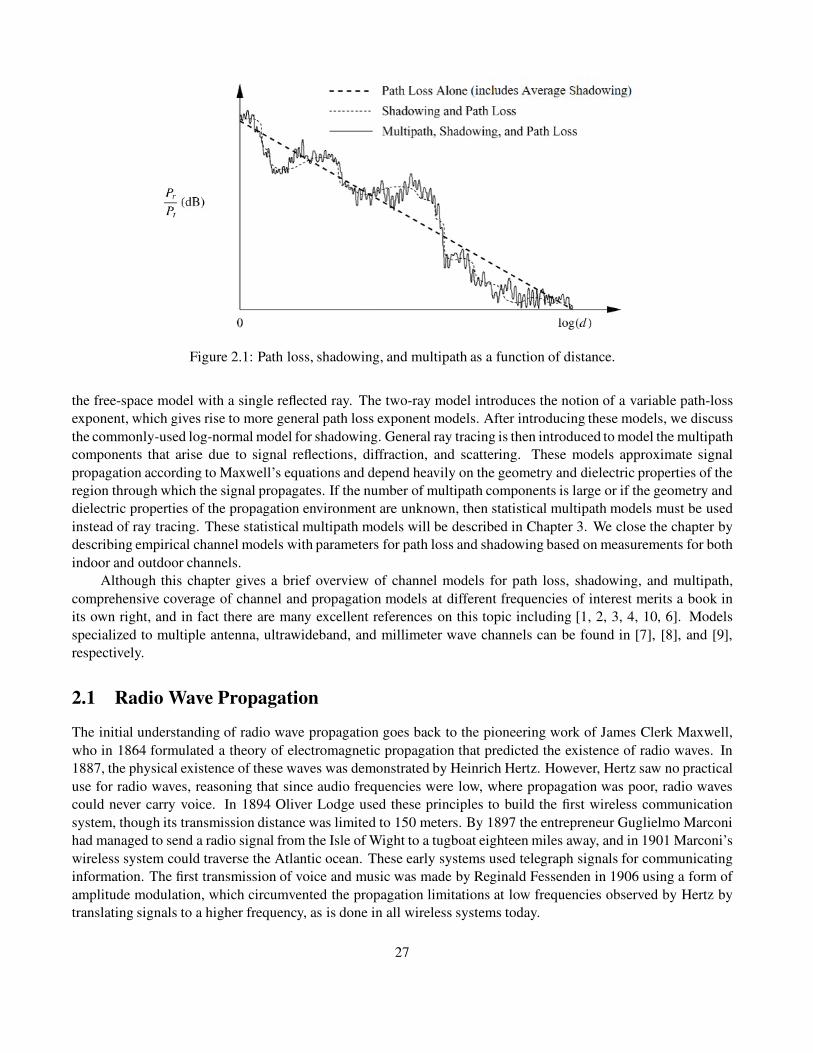
Figure 2.1: Path loss, shadowing, and multipath as a function of distance.

the free-space model with a single reflected ray. The two-ray model introduces the notion of a variable path-loss

exponent, which gives rise to more general path loss exponent models. After introducing these models, we discuss

the commonly-used log-normal model for shadowing. General ray tracing is then introduced to model the multipath

components that arise due to signal reflections, diffraction, and scattering. These models approximate signal

propagation according to Maxwell’s equations and depend heavily on the geometry and dielectric properties of the

region through which the signal propagates. If the number of multipath components is large or if the geometry and

dielectric properties of the propagation environment are unknown, then statistical multipath models must be used

instead of ray tracing. These statistical multipath models will be described in Chapter 3. We close the chapter by

describing empirical channel models with parameters for path loss and shadowing based on measurements for both

indoor and outdoor channels.

Although this chapter gives a brief overview of channel models for path loss, shadowing, and multipath,

comprehensive coverage of channel and propagation models at different frequencies of interest merits a book in

its own right, and in fact there are many excellent references on this topic including [1, 2, 3, 4, 10, 6]. Models

specialized to multiple antenna, ultrawideband, and millimeter wave channels can be found in [7], [8], and [9],

respectively.

2.1 Radio Wave Propagation

The initial understanding of radio wave propagation goes back to the pioneering work of James Clerk Maxwell,

who in 1864 formulated a theory of electromagnetic propagation that predicted the existence of radio waves. In

1887, the physical existence of these waves was demonstrated by Heinrich Hertz. However, Hertz saw no practical

use for radio waves, reasoning that since audio frequencies were low, where propagation was poor, radio waves

could never carry voice. In 1894 Oliver Lodge used these principles to build the first wireless communication

system, though its transmission distance was limited to 150 meters. By 1897 the entrepreneur Guglielmo Marconi

had managed to send a radio signal from the Isle of Wight to a tugboat eighteen miles away, and in 1901 Marconi’s

wireless system could traverse the Atlantic ocean. These early systems used telegraph signals for communicating

information. The first transmission of voice and music was made by Reginald Fessenden in 1906 using a form of

amplitude modulation, which circumvented the propagation limitations at low frequencies observed by Hertz by

translating signals to a higher frequency, as is done in all wireless systems today.

27

Electromagnetic waves propagate through environments where they are reflected, scattered, and diffracted

by walls, terrain, buildings, and other objects. The ultimate details of this propagation can be obtained by solving

Maxwell’s equations with boundary conditions that express the physical characteristics of these obstructing objects.

This often requires the calculation of the radar cross-section (RCS) of large and complex structures. Since these

calculations are difficult and since the necessary parameters are often not available, approximations have been

developed to characterize signal propagation without resorting to Maxwell’s equations.

The most common signal propagation approximations use ray-tracing techniques based on ray-optic theory

[10]. Ray-tracing approximates the propagation of electromagnetic waves by representing the wavefronts as dis-

crete narrow beams or rays. This approximation determines the reflection and refraction effects on the wavefront

but ignores the more complex scattering phenomenon predicted by Maxwell’s coupled differential equations. The

ray-tracing model most accurately approximates Maxwell’s equations when the wavelength of the signal is much

less than the size of the objects off of which it is reflected, refracted, or scattered. The simplest ray-tracing model is

the two-ray model, which accurately describes signal propagation when there is one direct path between the trans-

mitter and receiver and one reflected path. The reflected path typically bounces off the ground, and the two-ray

model is a good approximation for propagation along highways or rural roads and over water. We will analyze the

two-ray model in detail, as well as more complex models with additional reflected, scattered, or diffracted compo-

nents. Many propagation environments are not accurately characterized by ray-tracing models. In these cases it is

common to develop analytical models based on empirical measurements, and we will discuss several of the most

common of these empirical models.

Often the complexity and variability of the radio channel make it difficult to obtain an accurate deterministic

channel model. For these cases, statistical models are often used. The attenuation caused by signal path obstruc-

tions such as buildings or other objects is typically characterized statistically, as described in Section 2.7. Statistical

models are also used to characterize the constructive and destructive interference for a large number of multipath

components, as described in Chapter 3. Indoor environments tend to be less regular than outdoor environments,

since the geometric and dielectric characteristics change dramatically depending on whether the indoor environ-

ment is an open factory, cubicled office, or metal machine shop. For these environments computer-aided modeling

tools are available to predict signal propagation characteristics [11].

2.2 Transmit and Receive Signal Models

The transmitted and received signals in any wireless system are real-valued. The channel introduces an amplitude

and phase change at each frequency of the transmitted signal so that the received signal is also real-valued. Real

modulated and demodulated signals are often represented as the real part of a complex signal in order to facilitate

analysis. This model gives rise to the equivalent lowpass representation of bandpass signals, which we use for our

transmitted and received signals. More details on the equivalent lowpass representation of bandpass signals and

systems can be found in Appendix A.

We model the transmitted signal at carrier frequency fc as

s(t) = Re{u(t)ej2πfct}= Re{u(t)} cos(2πfct) − Im{u(t)} sin(2πfct)

= sI (t) cos(2πfct) − sQ(t) sin(2πfct), (2.1)

where u(t) = sI(t)+jsQ(t) is a complex baseband signal with in-phase component sI(t) = Re{u(t)}, quadrature

component sQ(t) = Im{u(t)}, bandwidth Bu, and power Pu. The signal u(t) is called the complex envelope or

equivalent lowpass signal of s(t). We call u(t) the complex envelope of s(t) because the magnitude of u(t) is the

magnitude of s(t). The phase of u(t) includes any carrier phase offset. The equivalent lowpass representation of

28

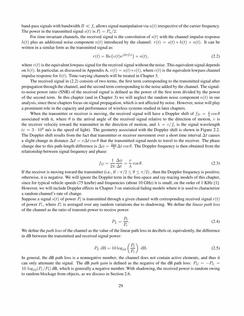
band-pass signals with bandwidthB � fc allows signal manipulation via u(t) irrespective of the carrier frequency.

The power in the transmitted signal s(t) is Pt = Pu/2.

For time-invariant channels, the received signal is the convolution of s(t) with the channel impulse response

h(t) plus an additional noise component n(t) introduced by the channel: r(t) = s(t) ∗ h(t) + n(t). It can be

written in a similar form as the transmitted signal as:

r(t) = Re{v(t)ej2πfct} + n(t), (2.2)

where v(t) is the equivalent lowpass signal for the received signal without the noise. This equivalent signal depends

on h(t). In particular, as discussed in Appendix A, v(t) = u(t)∗ c(t), where c(t) is the equivalent lowpass channel

impulse response for h(t). Time-varying channels will be treated in Chapter 3.

The received signal in (2.2) consists of two terms, the first term corresponding to the transmitted signal after

propagation through the channel, and the second term corresponding to the noise added by the channel. The signal-

to-noise power ratio (SNR) of the received signal is defined as the power of the first term divided by the power

of the second term. In this chapter (and in Chapter 3) we will neglect the random noise component n(t) in our

analysis, since these chapters focus on signal propagation, which is not affected by noise. However, noise will play

a prominent role in the capacity and performance of wireless systems studied in later chapters.

When the transmitter or receiver is moving, the received signal will have a Doppler shift of fD = vλ cos θ

associated with it, where θ is the arrival angle of the received signal relative to the direction of motion, v is

the receiver velocity toward the transmitter in the direction of motion, and λ = c/fc is the signal wavelength

(c = 3 · 108 m/s is the speed of light). The geometry associated with the Doppler shift is shown in Figure 2.2.

The Doppler shift results from the fact that transmitter or receiver movement over a short time interval ∆t causes

a slight change in distance ∆d = v∆t cos θ that the transmitted signal needs to travel to the receiver. The phase

change due to this path-length difference is ∆φ = 2πvλ ∆t cos θ. The Doppler frequency is then obtained from the

relationship between signal frequency and phase:

fD =1

2π

∆φ

∆t=v

λcos θ. (2.3)

If the receiver is moving toward the transmitter (i.e., if −π/2 ≤ θ ≤ π/2) , then the Doppler frequency is positive;

otherwise, it is negative. We will ignore the Doppler term in the free-space and ray-tracing models of this chapter,

since for typical vehicle speeds (75 km/hr) and frequencies (about 10 GHz) it is small, on the order of 1 KHz [1].

However, we will include Doppler effects in Chapter 3 on statistical fading models where it is used to characterize

a random channel’s rate of change.

Suppose a signal s(t) of power Pt is transmitted through a given channel with corresponding received signal r(t)

of power Pr, where Pr is averaged over any random variations due to shadowing. We define the linear path loss

of the channel as the ratio of transmit power to receive power:

PL =PtPr. (2.4)

We define the path loss of the channel as the value of the linear path loss in decibels or, equivalently, the difference

in dB between the transmitted and received signal power:

PL dB = 10 log10

(

PtPr

)

dB. (2.5)

In general, the dB path loss is a nonnegative number; the channel does not contain active elements, and thus it

can only attenuate the signal. The dB path gain is defined as the negative of the dB path loss: PG = −PL =

10 log10(Pr/Pt) dB, which is generally a negative number. With shadowing, the received power is random owing

to random blockage from objects, as we discuss in Section 2.6.

29

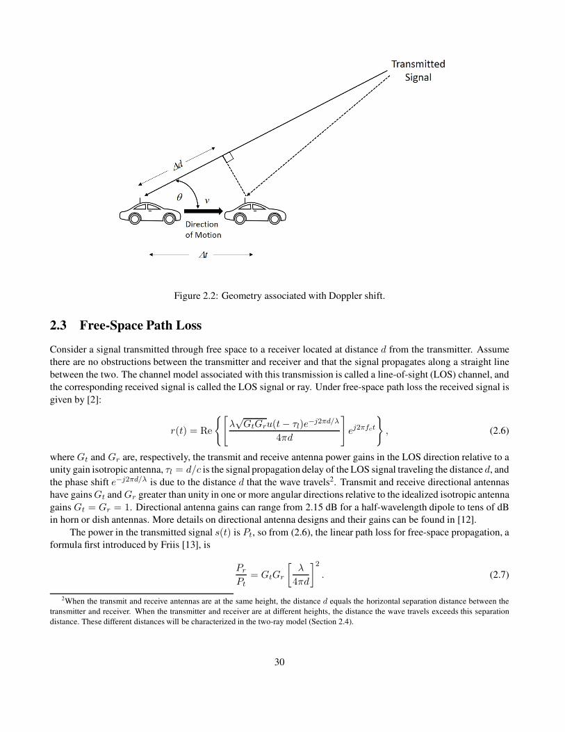
Figure 2.2: Geometry associated with Doppler shift.

2.3 Free-Space Path Loss

Consider a signal transmitted through free space to a receiver located at distance d from the transmitter. Assume

there are no obstructions between the transmitter and receiver and that the signal propagates along a straight line

between the two. The channel model associated with this transmission is called a line-of-sight (LOS) channel, and

the corresponding received signal is called the LOS signal or ray. Under free-space path loss the received signal is

given by [2]:

r(t) = Re

{[

λ√GtGru(t− τl)e

−j2πd/λ

4πd

]

ej2πfct

}

, (2.6)

where Gt and Gr are, respectively, the transmit and receive antenna power gains in the LOS direction relative to a

unity gain isotropic antenna, τl = d/c is the signal propagation delay of the LOS signal traveling the distance d, and

the phase shift e−j2πd/λ is due to the distance d that the wave travels2. Transmit and receive directional antennas

have gainsGt and Gr greater than unity in one or more angular directions relative to the idealized isotropic antenna

gains Gt = Gr = 1. Directional antenna gains can range from 2.15 dB for a half-wavelength dipole to tens of dB

in horn or dish antennas. More details on directional antenna designs and their gains can be found in [12].

The power in the transmitted signal s(t) is Pt, so from (2.6), the linear path loss for free-space propagation, a

formula first introduced by Friis [13], is

PrPt

= GtGr

[

λ

4πd

]2

. (2.7)

2When the transmit and receive antennas are at the same height, the distance d equals the horizontal separation distance between the

transmitter and receiver. When the transmitter and receiver are at different heights, the distance the wave travels exceeds this separation

distance. These different distances will be characterized in the two-ray model (Section 2.4).

30

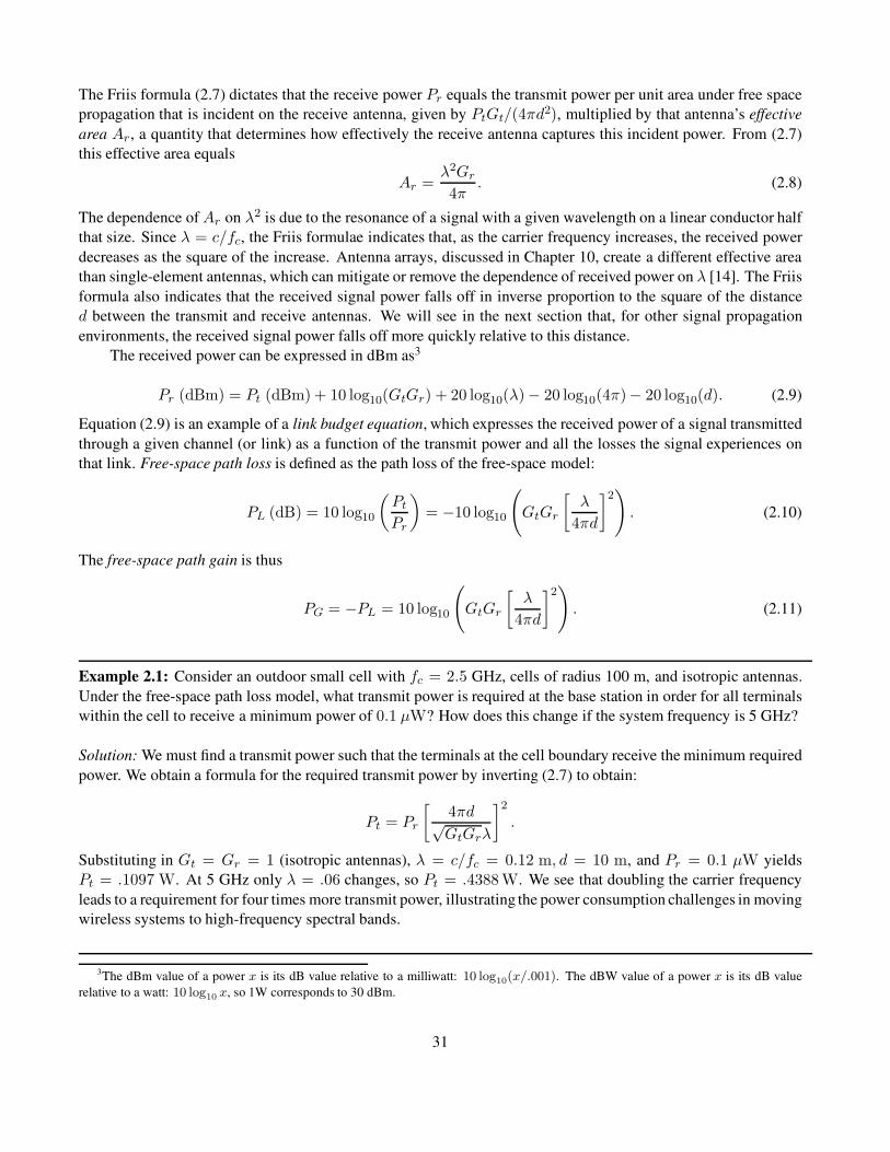
The Friis formula (2.7) dictates that the receive power Pr equals the transmit power per unit area under free space

propagation that is incident on the receive antenna, given by PtGt/(4πd2), multiplied by that antenna’s effective

area Ar, a quantity that determines how effectively the receive antenna captures this incident power. From (2.7)

this effective area equals

Ar =λ2Gr4π

. (2.8)

The dependence ofAr on λ2 is due to the resonance of a signal with a given wavelength on a linear conductor half

that size. Since λ = c/fc, the Friis formulae indicates that, as the carrier frequency increases, the received power

decreases as the square of the increase. Antenna arrays, discussed in Chapter 10, create a different effective area

than single-element antennas, which can mitigate or remove the dependence of received power on λ [14]. The Friis

formula also indicates that the received signal power falls off in inverse proportion to the square of the distance

d between the transmit and receive antennas. We will see in the next section that, for other signal propagation

environments, the received signal power falls off more quickly relative to this distance.

The received power can be expressed in dBm as3

Pr (dBm) = Pt (dBm) + 10 log10(GtGr) + 20 log10(λ)− 20 log10(4π)− 20 log10(d). (2.9)

Equation (2.9) is an example of a link budget equation, which expresses the received power of a signal transmitted

through a given channel (or link) as a function of the transmit power and all the losses the signal experiences on

that link. Free-space path loss is defined as the path loss of the free-space model:

PL (dB) = 10 log10

(

PtPr

)

= −10 log10

(

GtGr

[

λ

4πd

]2)

. (2.10)

The free-space path gain is thus

PG = −PL = 10 log10

(

GtGr

[

λ

4πd

]2)

. (2.11)

Example 2.1: Consider an outdoor small cell with fc = 2.5 GHz, cells of radius 100 m, and isotropic antennas.

Under the free-space path loss model, what transmit power is required at the base station in order for all terminals

within the cell to receive a minimum power of 0.1 µW? How does this change if the system frequency is 5 GHz?

Solution: We must find a transmit power such that the terminals at the cell boundary receive the minimum required

power. We obtain a formula for the required transmit power by inverting (2.7) to obtain:

Pt = Pr

[

4πd√GtGrλ

]2

.

Substituting in Gt = Gr = 1 (isotropic antennas), λ = c/fc = 0.12 m, d = 10 m, and Pr = 0.1 µW yields

Pt = .1097 W. At 5 GHz only λ = .06 changes, so Pt = .4388 W. We see that doubling the carrier frequency

leads to a requirement for four times more transmit power, illustrating the power consumption challenges in moving

wireless systems to high-frequency spectral bands.

3The dBm value of a power x is its dB value relative to a milliwatt: 10 log10(x/.001). The dBW value of a power x is its dB value

relative to a watt: 10 log10 x, so 1W corresponds to 30 dBm.

31

2.4 Two-Ray Multipath Model

The two-ray model is used when a single ground (or other) reflection dominates the multipath effect, as illustrated

in Figure 2.3. The received signal consists of two components: the LOS component or ray, which corresponds to

the transmitted signal propagating through free space, and a reflected component or ray, which is the transmitted

signal reflected off the ground. The received LOS ray is given by the free-space propagation loss formula (2.6)

with the distance the signal travels set to d0. The reflected ray shown in Figure 2.3 travels distance d1 = d11 +d12.

Since the two signal components in this model travel different distances, we use d in this model and all subsequent

propagation models in this chapter to denote the horizontal distance between the transmitter and receiver. The

distances d0 and d1 then depend on d as well as the transmitter and receiver heights ht and hr. We see from Figure

2.3 that when ht = hr, d = d0, and when d is very large relative to ht and hr, d ≈ d0 ≈ d1.

If we ignore the effect of surface wave attenuation4 then, by superposition, the received signal for the two-ray

model is

r2-ray(t) = Re

{

λ

4π

[√G0u(t− τ0)e

−j2πd0/λ

d0+R√G1u(t− τ1)e

−j2πd1/λ

d1

]

ej2πfct

}

, (2.12)

where τ0 = d0/c is the time delay of the LOS ray, τ1 = d1/c is the time delay of the ground reflection ray,√G0 =

√

Gt0Gr0 is the product of the transmit and receive antenna field radiation patterns in the LOS direction,

R is the ground reflection coefficient, and√G1 =

√

Gt1Gr1 is the product of the transmit and receive antenna

field radiation patterns corresponding to the ground reflection. The delay spread of the two-ray model equals the

difference between the delay of the LOS ray and that of the reflected ray: (d1 − d0)/c.

If the transmitted signal is narrowband relative to the delay spread such that (τ1−τ0 � B−1u ) then u(t−τ1) ≈

u(t− τ0). With this approximation, the received power of the two-ray model for narrowband transmission is

Figure 2.3: Two-ray model.

Pr = Pt

[

λ

4π

]2 ∣∣

∣

∣

√G0

d0+R√G1e

−j∆φ

d1

∣

∣

∣

∣

2

, (2.13)

where ∆φ = 2π(d1 − d0)/λ is the phase difference between the two received signal components. Equation

(2.13) has been shown [15] to agree closely with empirical data. From the geometry of the two-ray model, d1 =√

(ht + hr)2 + d2 and x0 =√

(ht − hr)2 + d2. Hence

d1 − d0 =√

(ht + hr)2 + d2 −√

(ht − hr)2 + d2. (2.14)

4This is a valid approximation for antennas located more than a few wavelengths from the ground.

32

When d is very large compared to ht + hr , we can use a Taylor series approximation in (2.14) to get

∆φ =2π

λ

(

√

(ht + hr)2 + d2 −√

(ht − hr)2 + d2)

≈ 4πhthrλd

. (2.15)

The ground reflection coefficient is given by [1, 16]

R =sin θ − Z

sin θ + Z, (2.16)

where

Z =

{√εr − cos2 θ/εr for vertical polarization,√εr − cos2 θ for horizontal polarization,

(2.17)

and εr is the dielectric constant of the ground. For earth or road surfaces this dielectric constant is approximately

that of a pure dielectric (for which εr is real with a value of about 15).

Since for asymptotically large d, d1 ≈ d0 ≈ d, G1 ≈ G0 where we denote this approximate antenna gain as

G, and θ ≈ 0 which by (2.16) then implies that R ≈ −1. Substituting these approximations into (2.13) yields

Pr ≈[

λ√G

4πd

]2

|1− e−j∆φ|2Pt. (2.18)

Using the approximation for ∆φ in (2.15) at large dh we get the final approximation for received power at

large distance d as

Pr ≈[

λ√G

4πdh

]2 [4πhthrλd

]2

Pt =

[√Ghthrd2

]2

Pt, (2.19)

or, in dB,

Pr dBm = Pt dBm + 10 log10(G) + 20 log10(hthr) − 40 log10(d). (2.20)

Thus, in the limit of asymptotically large d, the received power falls off inversely with the fourth power of d and is

independent of the wavelength λ. This is in contrast to free-space propagation where power is inversely proportion

to d2 and proportional to λ2. The received signal power becomes independent of λ because directional antenna

arrays have a received power that does not necessarily decrease with λ, and combining the direct path and reflected

signal at the receiver effectively forms an antenna array.

A plot of (2.13) as a function of the transmit-receive separation distance d is shown in Figure 2.4 for fc = 900MHz, R = −1, ht = 50 m, hr = 2 m, G0 = G1 = 1, and received power normalized to 0 dB at a reference

distance of 1 m. This plot reflects the case where the transmit antenna height ht is much larger than the receiver

antenna height hr, as is typical in an urban cellular system where macrocell base stations are located on top of

tall buildings with mobile devices near street level. The plot can be separated into three segments. For small

distances (d < ht) the two rays add constructively as d increases from zero. The local maximum over this

segment occurs for d such that ∆φ = π in (2.15). At that distance the phases of the two multipath components

are perfectly aligned (Re−j∆φ = 1). The path loss over this segment is roughly proportional to 1/(d2 + h2t )

since, at these small distances, the distance between the transmitter and receiver is x0 =√

d2 + (ht − hr)2; thus

(1/x0)2 ≈ 1/(d2 + h2

t ) since ht � hr. After this first local maximum and up to a certain critical distance dc,

the wave experiences constructive and destructive interference of the two rays as ∆φ changes with d, resulting in

a wave pattern with a sequence of maxima (when |∆φ| is an odd integer multiple of π) and minima (when |∆φ|

33

Figure 2.4: Received power versus distance for two-ray model. The received power is normalized to 0 dB at a

reference distance of 1 m.

is an even integer multiple of 2π). These maxima and minima are also referred to as multipath fading, discussed

in more detail in the next chapter. At the critical distance dc, the final maximum is reached, after which the signal

power falls off proportionally with d−4. This rapid falloff with distance is due to the fact that, for d > dc, the

signal components only combine destructively since ∆φ→ 0 as d→ ∞. Since the final maximum is achieved for

d such that ∆φ = π, an approximation for dc can be obtained by setting ∆φ = π in (2.15), obtaining

dc = 4hthr/λ. (2.21)

For the parameters used to generate Figure 2.4, dc = 1.2 Km (log10 dc = 3.08), which is also shown in the figure.

The power falloff with distance in the two-ray model can be approximated by averaging out its local maxima

and minima. This results in a piecewise linear model with three segments, which is also shown in Figure 2.4

slightly offset from the actual power falloff curve for illustration purposes. In the first segment, in order to get a

constant power falloff we assume x0 ≈ x1 = x+ x′ ≈ h2t , leading to a power falloff proportional to 1/h2

t that is

independent of d; for distances between ht and dc, power falls off at −20 dB/decade; and at distances greater than

dc, power falls off at –40 dB/decade.

The critical distance dc is proportional to the transmit antenna height ht and to the carrier frequency fc = c/λ.

Thus, for small cells and indoor systems where ht is ten meters or less, for fc on the order of 1 GHz, dc is hundreds

of meters, as illustrated in Example 2.2. On the other hand, for millimeter wave systems where fc is tens of GHz,

dc typically well exceeds a kilometer. The value of dc can be used for system design. For example, if propagation

in a cellular system obeys the two-ray model then the critical distance would be a natural size for the cell radius,

since the path loss associated with interference outside the cell would be much larger than path loss for desired

signals inside the cell. However, setting the cell radius to dc could result in very large cells, as illustrated in Figure

2.4 and in the next example. Since smaller cells are more desirable – both to increase capacity and reduce transmit

power – cell radii are typically much smaller than dc. Thus, with a two-ray propagation model, power falloff within

34

these relatively small cells goes as distance squared. Moreover, propagation in cellular systems rarely follows a

two-ray model, since cancellation by reflected rays rarely occurs in all directions.

Example 2.2: Determine the critical distance for the two-ray model in an outdoor cell with ht = 10 m, hr = 3 mand in an indoor cell with ht = 3 m, hr = 2 m for fc = 2 GHz.

Solution: dc = 4hthr/λ = 800 m for the outdoor cell and 160 m for the indoor cell. A cell radius of 800 m in

an outdoor cell is typical for a macrocell but a bit large for a small cell which today are on the order of 10-100 mto maintain large capacity. However, for a macrocell with an 800 m radius under these system parameters, signal

power would fall off as d2 inside the cell, while interference from neighboring cells would fall off as d4 and thus

would be greatly reduced. Similarly, 160 m is quite large for the cell radius of an indoor system, as there would

typically be many walls the signal would have to penetrate for an indoor cell radius of that size. Hence an indoor

system would typically have a smaller cell radius: on the order of 10–20 m, the size of one room or a few adjacent

rooms in a typical building.

2.5 Path Loss Exponent Models

2.5.1 Single-Slope

The complexity of signal propagation makes it difficult to obtain a single model that characterizes path loss accu-

rately across a range of different environments and frequencies. Accurate path loss models can be obtained from

complex analytical models or empirical measurements when tight system specifications must be met or the best

locations for base stations or access-point layouts must be determined. However, for general trade-off analysis of

various system designs it is sometimes best to use a simple model that captures the essence of signal propagation

without resorting to complicated path loss models, which are only approximations to the real channel anyway.

The following single-slope model for path loss as a function of distance is a simple model that captures several

important propagation characteristics.

Pr = PtK

[

drd

]γ

, (2.22)

where dr is a reference distance for the antenna far field, γ is the path-loss exponent, and K is a unitless constant

equal to the path gain Pr/Pt at distance d = dr. The dB attenuation is thus

Pr (dBm) = Pt (dBm) +K dB − 10γ log10 (d/dr) , (2.23)

and the path loss consists of two terms, where all environment and antenna parameters are captured by the first

term, and the path loss due only to distance is captured by the second term:

PL (dB) = 10 log10 (Pt/Pr) = −10 log10K + 10γ log10(d/dr). (2.24)

The values for K, dr, and γ can be obtained to approximate either an analytical or empirical model. In

particular, the free-space path-loss model and some of the empirical models described in Section 2.7 are all of the

same form as (2.23). Because of antenna near field effects at transmit distances on the order of a signal wavelength,

the model (2.23) is generally valid only at transmission distances d > dr, where dr is typically assumed to be 1 mfor systems transmitting over distances greater than this nominal value.

35

Table 2.1: Typical path loss exponents

Environment γ range

Urban macrocells 3.7–6.5

Urban microcells 2.7–3.5

Office building (same floor) 1.6–3.5

Office building (multiple floors) 2–6

Store 1.8–2.2

Factory 1.6–3.3

Home 3

When the single-slope model is used to approximate empirical measurements, the value of K < 1 is some-

times set to the free-space path gain at distance dr assuming isotropic antennas:

K dB = 20 log10

λ

4πdr, (2.25)

and this assumption is supported by empirical data for free-space path loss at a transmission distance of 100 m [17].

Alternatively,K can be determined by measurement at dr or optimized (alone or together with γ) to minimize the

mean-square error (MSE) between the model and the empirical measurements [17]. The value of γ depends on the

propagation environment: for propagation that approximately follows a free-space or two-ray model, γ is set to 2 or

4 respectively. The value of γ for more complex environments can be obtained via a minimum mean-square error

(MMSE) fit to empirical measurements, as illustrated in Example 2.3. Alternatively, γ can be obtained from an

empirically based model that takes into account frequency and antenna height [17]. Table 2.6 summarizes values

of the path loss exponent γ for different environments based on data from [11, 17, 18, 19, 20, 21, 52]. Empirical

measurements indicate that path loss exponents at higher frequencies tend to be higher [19, 23, 21, 22, 57, 59]

whereas path loss exponents at higher antenna heights tend to be lower [17, 57, 59]. The more complex empirical

models described below in Section 2.7, particularly the widely used 3GPP and WINNER II channel models [57,

59], have additional terms that explicitly capture the dependence of path loss on frequency and antenna height.

Note that the wide range of empirical path-loss exponents for indoor propagation may be due to attenuation caused

by floors, objects, and partitions (see Section 2.5.5).

Example 2.3: Consider the set of empirical measurements of Pr/Pt given in Table 2.2 for an indoor system at 900

MHz. Find the path loss exponent γ that minimizes the MSE between the single-slope model (2.23) and the empir-

ical dB power measurements, assuming that dr = 1 m and K is determined from the free-space path-gain formula

at this dr. Find the received power at 150 m for the single-slope path loss model with this path loss exponent and a

transmit power of 1 mW (0 dBm). Note that, since the path loss model in dB is linear, minimizing the MSE of the

empirical data in dB (versus in linear units) relative to this model is a simple linear regression.

Solution: We first set up the MMSE error equation for the dB power measurements as

F (γ) =5∑

i=1

[Mmeasured(di) −Mmodel(di)]2,

where Mmeasured(di) is the path loss measurement in Table 2.2 at distance di and where Mmodel(di) = K −10γ log10(d) is the path loss at di based on (2.23). Now using the free-space path gain formula yields K =

20 log10(.3333/(12π)) = −31.53 dB. Thus

36

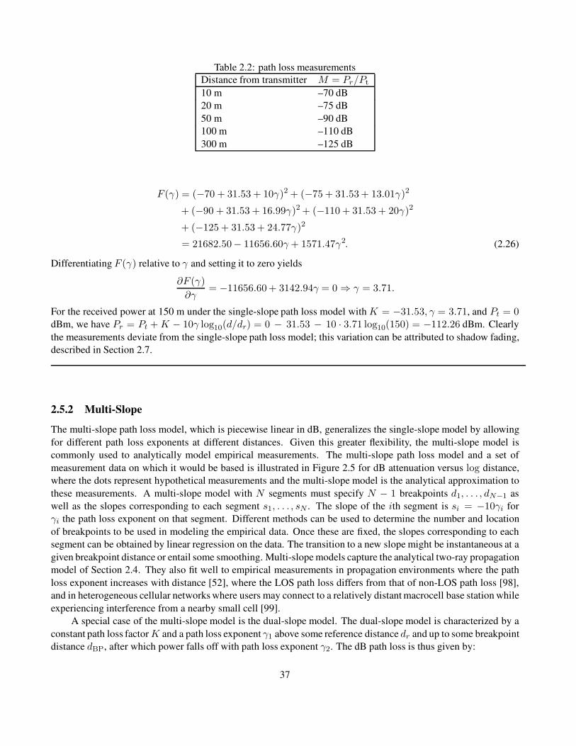
Table 2.2: path loss measurements

Distance from transmitter M = Pr/Pt

10 m –70 dB

20 m –75 dB

50 m –90 dB

100 m –110 dB

300 m –125 dB

F (γ) = (−70 + 31.53 + 10γ)2 + (−75 + 31.53 + 13.01γ)2

+ (−90 + 31.53 + 16.99γ)2 + (−110 + 31.53 + 20γ)2

+ (−125 + 31.53 + 24.77γ)2

= 21682.50− 11656.60γ+ 1571.47γ2. (2.26)

Differentiating F (γ) relative to γ and setting it to zero yields

∂F (γ)

∂γ= −11656.60 + 3142.94γ = 0 ⇒ γ = 3.71.

For the received power at 150 m under the single-slope path loss model with K = −31.53, γ = 3.71, and Pt = 0dBm, we have Pr = Pt +K − 10γ log10(d/dr) = 0 − 31.53 − 10 · 3.71 log10(150) = −112.26 dBm. Clearly

the measurements deviate from the single-slope path loss model; this variation can be attributed to shadow fading,

described in Section 2.7.

2.5.2 Multi-Slope

The multi-slope path loss model, which is piecewise linear in dB, generalizes the single-slope model by allowing

for different path loss exponents at different distances. Given this greater flexibility, the multi-slope model is

commonly used to analytically model empirical measurements. The multi-slope path loss model and a set of

measurement data on which it would be based is illustrated in Figure 2.5 for dB attenuation versus log distance,

where the dots represent hypothetical measurements and the multi-slope model is the analytical approximation to

these measurements. A multi-slope model with N segments must specify N − 1 breakpoints d1, . . . , dN−1 as

well as the slopes corresponding to each segment s1, . . . , sN . The slope of the ith segment is si = −10γi for

γi the path loss exponent on that segment. Different methods can be used to determine the number and location

of breakpoints to be used in modeling the empirical data. Once these are fixed, the slopes corresponding to each

segment can be obtained by linear regression on the data. The transition to a new slope might be instantaneous at a

given breakpoint distance or entail some smoothing. Multi-slope models capture the analytical two-ray propagation

model of Section 2.4. They also fit well to empirical measurements in propagation environments where the path

loss exponent increases with distance [52], where the LOS path loss differs from that of non-LOS path loss [98],

and in heterogeneous cellular networks where users may connect to a relatively distant macrocell base station while

experiencing interference from a nearby small cell [99].

A special case of the multi-slope model is the dual-slope model. The dual-slope model is characterized by a

constant path loss factorK and a path loss exponent γ1 above some reference distance dr and up to some breakpoint

distance dBP, after which power falls off with path loss exponent γ2. The dB path loss is thus given by:

37

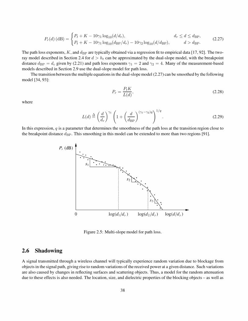
Pr(d) (dB) =

{

Pt +K − 10γ1 log10(d/dr), dr ≤ d ≤ dBP,

Pt +K − 10γ1 log10(dBP/dr) − 10γ2 log10(d/dBP), d > dBP.(2.27)

The path loss exponents,K, and dBP are typically obtained via a regression fit to empirical data [17, 92]. The two-

ray model described in Section 2.4 for d > ht can be approximated by the dual-slope model, with the breakpoint

distance dBP = dc given by (2.21) and path loss exponents γ1 = 2 and γ2 = 4. Many of the measurement-based

models described in Section 2.9 use the dual-slope model for path loss.

The transition between the multiple equations in the dual-slope model (2.27) can be smoothed by the following

model [34, 93]:

Pr =PtK

L(d), (2.28)

where

L(d)∆=

(

d

dr

)γ1(

1 +

(

d

dBP

)(γ1−γ2)q)1/q

. (2.29)

In this expression, q is a parameter that determines the smoothness of the path loss at the transition region close to

the breakpoint distance dBP. This smoothing in this model can be extended to more than two regions [91].

Figure 2.5: Multi-slope model for path loss.

2.6 Shadowing

A signal transmitted through a wireless channel will typically experience random variation due to blockage from

objects in the signal path, giving rise to random variations of the received power at a given distance. Such variations

are also caused by changes in reflecting surfaces and scattering objects. Thus, a model for the random attenuation

due to these effects is also needed. The location, size, and dielectric properties of the blocking objects – as well as

38

the changes in reflecting surfaces and scattering objects that cause the random attenuation – are generally unknown,

so statistical models must be used to characterize this attenuation.

The most common model for this additional attenuation is log-normal shadowing; under this model the dB

value of the random attenuation is Gauss-distributed. The log-normal shadowing model has been empirically con-

firmed to model accurately the variation in received power in both outdoor and indoor radio propagation environ-

ments (see, e.g., [17, 102]). In the log-normal shadowing model, the ratio of transmit-to-receive power ψ = Pt/Pris assumed to be random with a log-normal distribution given by

p(ψ) =ξ√

2πσψdBψ

exp

[

−(10 log10 ψ − µψdB)2

2σ2ψdB

]

, ψ > 0, (2.30)

where ξ = 10/ ln10, µψdBis the mean of ψdB = 10 log10 ψ in decibels, and σψdB

is the standard deviation of

ψdB (also in dB). The mean can be based on an analytical model or empirical measurements. For empirical mea-

surements µψdBequals the empirical path loss, since average attenuation from shadowing is already incorporated

into the measurements. For analytical models, µψdBmust incorporate both the path loss (e.g., from a free-space or

ray-tracing model) as well as average attenuation from blockage. Alternatively, path loss can be treated separately

from shadowing, as described in the next section.

A random variable with a log-normal distribution is called a log-normal random variable. Note that if ψ

is log-normal then the received power and received SNR will also be log-normal, since these are just constant

multiples of ψ. For received SNR the mean and standard deviation of this log-normal random variable are also in

decibels. For log-normal received power the random variable has units of power, so its mean and standard deviation

will be in dBm or dBW instead of dB. The mean of ψ (the linear average path gain) can be obtained from (2.30) as

µψ = E[ψ] = exp

[

µψdB

ξ+σ2ψdB

2ξ2

]

. (2.31)

The conversion from the linear mean (in dB) to the log mean (in dB) is derived from (2.31) as

10 log10 µψ = µψdB+σ2ψdB

2ξ. (2.32)

Performance in log-normal shadowing is typically parameterized by the log mean µψdB, which is referred to

as the average dB path loss and is given in units of dB. With a change of variables we see that the distribution of

the dB value of ψ is Gaussian with mean µψdBand standard deviation σψdB:

p(ψdB) =1√

2πσψdB

exp

[

−(ψdB − µψdB)2

2σ2ψdB

]

. (2.33)

The log-normal distribution of ψ or, equivalently, the Gaussian distribution of ψdB is defined by two parameters:

µψdBand σψdB

. Given that ψdB is based on the ratio of transmit and receive powers, it can be expressed as a

difference of these powers in either dBW or dBm, as follows:

ψdB = 10 log10(Pt/Pr) = Pt dBW − Pr dBW = Pt dBm − Pr dBm. (2.34)

Since ψdB is Gauss-distributed, by (2.34) and properties of Gaussian random variables we have that Pr dBW is

also Gauss-distributed with mean Pt dBW− µψdBand standard deviation σψdB, i.e. the same standard deviation as

ψdB. Similarly, Pr dBm is Gauss-distributed with mean Pt dBm − µψdBand standard deviation σψdB.

The log-normal distribution is an imperfect approximation to the effect of shadowing because it has a non-zero

probability that the received power exceeds the transmit power, which violates the laws of physics. In particular,

39

since the transmit power should always exceed the received power, ψ = Pt/Pr should always be greater than unity.

Thus shadowing models set µψdBto be greater than zero. Note, however, that the log-normal distribution (2.30)

takes values for 0 ≤ ψ ≤ ∞. Hence, for ψ < 1 we have Pr > Pt, which is physically impossible. However, this

probability will be very small when µψdBis large and positive. Thus, the log-normal model captures the underlying

physical model for shadowing most accurately when µψdB� 0.

If the mean and standard deviation for the shadowing model are based on empirical measurements, then the

question arises as to whether they should be obtained by taking averages of the linear or rather the dB values of the

empirical measurements. In other words, given empirical (linear) path loss measurements {pi}Ni=1, should the mean

path loss be determined as µψ = (1/N )∑Ni=1 pi or as µψdB

= (1/N )∑N

i=1 10 log10 pi? A similar question arises

for computing the empirical variance. In practice it is more common to determine mean path loss and variance

based on averaging the dB values of the empirical measurements for several reasons. First, as we shall see, the

mathematical justification for the log-normal model is based on dB measurements. In addition, the literature

shows that obtaining empirical averages based on dB path loss measurements leads to a better approximation for

the physical channel being modeled [103]. Finally, as we saw in Section 2.5.4, power falloff with distance models

are often obtained by a piecewise linear approximation to empirical measurements of dB power versus the log of

distance [11].

Most empirical studies for outdoor channels support a standard deviation σψdBranging from 4 dB to 13 dB

[1, 34, 104, 105, 106]. Larger deviations are associated with environments that contain a high density of blocking

objects such as buildings and foliage outdoors, or walls and furniture indoors. Moreover, since attenuation by ob-

jects is more severe and more variable at high frequencies, and there is more variance in the number of attenuating

objects at large distances, σψdBgenerally increases with both frequency and distance [72].The mean power µψdB

depends on the path loss and building properties in the area under consideration. The mean power µψdBvaries with

distance; this is due to path loss and to the fact that average attenuation from objects increases with distance owing

to the potential for a larger number of attenuating objects.

The Gaussian model for the distribution of the mean received signal in dB can be justified by the following

attenuation model when shadowing is dominated by the attenuation from blocking objects. The attenuation of a

signal as it travels through an object of depth d is approximately equal to

s(d) = e−αd, (2.35)

where α is an attenuation constant that depends on the object’s materials and dielectric properties. If we assume

that α is approximately equal for all blocking objects and that the ith blocking object has a random depth di, then

the attenuation of a signal as it propagates through this region is

s(dt) = e−αΣidi = e−αdt , (2.36)

where dt =∑

i di is the sum of the random object depths through which the signal travels. If there are many

objects between the transmitter and receiver, then by the cental limit theorem we can approximate dt by a Gaussian

random variable. Thus, ln s(dt) = −αdt will have a Gaussian distribution with mean µ and standard deviation σ.

The value of σ will depend on the environment.

Example 2.4: In Example 2.3 we found that the exponent for the single-slope path loss model that best fits the

measurements in Table 2.2 was γ = 3.71. Assuming the single-slope path loss model with this exponent and the

same K = −31.53 dB, find σ2ψdB

, the variance of log-normal shadowing about the mean path loss based on these

empirical measurements.

Solution:

40

The sample variance relative to the simplified path loss model with γ = 3.71 is

σ2ψdB

=1

5

5∑

i=1

[Mmeasured(di) −Mmodel(di)]2,

where Mmeasured(di) is the path loss measurement in Table 2.2 at distance di and Mmodel(di) = K −37.1 log10(d).

This yields

σ2ψdB

=1

5[(−70 + 31.53 + 37.1)2 + (−75 + 31.53 + 48.27)2

+ (−90 + 31.53 + 63.03)2 + (−110 + 31.53 + 74.2)2

+ (−125 + 31.53 + 91.90)2]

= 13.28.

Thus, the standard deviation of shadow fading on this path is σψdB= 3.64 dB. Note that the bracketed term in the

displayed expression equals the MMSE formula (2.26) from Example 2.3 with γ = 3.71.

Extensive measurements have been taken to characterize the empirical autocorrelation function of the shadow

fading process over distance for different environments at different frequencies (see e.g. [105, 107, 108, 109,

110]). The most common analytical model for this function, first proposed by Gudmundson [105] and based

on empirical measurements, assumes that the shadowing ψ(d) is a first-order autoregressive process where the

covariance between shadow fading at two points separated by distance δ is characterized by

A(δ) = E[(ψdB(d)− µψdB)(ψdB(d+ δ)− µψdB

)] = σ2ψdBρδ/DD , (2.37)

where ρD is the normalized covariance between two points separated by a fixed distance D. This covariance

must be obtained empirically, and it varies with the propagation environment and carrier frequency. Measurements

indicate that for suburban macrocells with fc = 900 MHz, ρD = 0.82 for D = 100 m and for urban microcells

with fc = 2 GHz, ρD = 0.3 for D = 10 m [105, 109]. This model can be simplified and its empirical dependence

removed by setting ρD = 1/e for distanceD = Xc, which yields

A(δ) = σ2ψdB

e−δ/Xc . (2.38)

The decorrelation distance Xc in this model is the distance at which the signal autocovariance equals 1/e of its

maximum value and is on the order of the size of the blocking objects or clusters of these objects. For outdoor

systems,Xc typically ranges from 50 m to 100 m [108, 109]. For users moving at velocity v, the shadowing decor-

relation in time τ is obtained by substituting vτ = δ in (2.37) or (2.38). For a linear array of antennas, discussed

in Chapter 10, shadowing can vary with the angle between the array and the signal’s LOS path. Autocorrelation

relative to this angle has been investigated in [107, 109].

The first-order autoregressive correlation model (2.37) and its simplified form (2.38) are easy to analyze and

to simulate. Specifically, one can simulate ψdB by first generating a white Gaussian noise process with power

σ2ψdB

and then passing it through a first-order filter with response ρδ/DD for a covariance characterized by (2.37)

or response e−δ/Xc for a covariance characterized by (2.38). The filter output will produce a shadowing random

process with the desired correlation properties [105, 106].

41

2.7 Combined Path Loss and Shadowing

Models for path loss and shadowing can be combined to capture power falloff versus distance along with the

random attenuation about this path loss from shadowing. In this combined model, average dB path loss (µψdB) is

characterized by the path loss model while shadow fading, with a mean of 0 dB, creates variations about this path

loss, as illustrated by the path loss and shadowing curve in Figure 2.1. Specifically, this curve plots the combination

of the single-slope path loss model (2.22) and the log-normal shadowing random process defined by (2.33) and

(2.38).

2.7.1 Single-Slope Path Loss with Log-Normal Shadowing

For the combined model of single-slope path loss (2.23) and log-normal shadowing (2.32), the ratio of received to

transmitted power in dB is given by

PrPt

dB = 10 log10K − 10γ log10 (d/dr) − ψdB, (2.39)

where ψdB is a Gauss-distributed random variable with variance σ2ψdB

. The mean of ψdB is assumed to be zero when

the term 10 log10K captures average shadowing. When this is not the case, for example whenK is calculated from

the free-space path gain formula at d = dr, then the mean of ψdB is positive and equal to the average shadowing

loss over all distances. In (2.39), and as shown in Figure 2.1, the path loss decreases linearly relative to log10 d/drwith a slope of −10γ dB/decade, where γ is the path loss exponent. The variations due to shadowing change more

rapidly, on the order of the decorrelation distanceXc.

Examples 2.3 and 2.4 illustrated the combined model for single-slope path loss and log-normal shadow-

ing based on the measurements in Table 2.2, where path loss obeys the single-slope path loss model with K =

−31.53 dB and path loss exponent γ = 3.71 and where shadowing obeys the log-normal model with mean given

by the path loss model and standard deviation σψdB= 3.65 dB.

2.7.2 Outage Probability

The combined effects of path loss and shadowing have important implications for wireless system design. In

wireless systems there is typically a target minimum received power level Pmin below which performance becomes

unacceptable (e.g., the caller’s voice on a cell phone is unintelligible). However, with shadowing the received

power at any given distance from the transmitter is log-normally distributed with some probability of falling below

Pmin. We define outage probability Pout(Pmin, d) to be the probability that the received power at a given distance

d, Pr(d), falls below Pmin: Pout(Pmin, d) = p(Pr(d) < Pmin). For the combined path loss and shadowing model of

Section 2.8 this becomes

p(Pr(d) ≤ Pmin) = 1 − Q

(

Pmin − (Pt + 10 log10K − 10γ log10(d/dr))

σψdB

)

, (2.40)

where the Q-function is defined as the probability that a Gaussian random variable X with mean 0 and variance 1

is greater than z:

Q(z) , p(X > z) =

∫ ∞

z

1√2πe−y

2/2dy. (2.41)

The conversion between the Q-function and complementary error function is

Q(z) =1

2erfc

(

z√2

)

. (2.42)

42

We will omit the arguments Pmin and d of Pout when the context is clear or in generic references to outage proba-

bility.

Example 2.5: Find the outage probability at 150 m for a channel based on the single-slope path loss and shadowing

models of Examples 2.3 and 2.4, assuming a transmit power of Pt = 10 mW and minimum power requirement of

Pmin = −110.5 dBm.

Solution: We have Pt = 10 mW = 10 dBm. Hence,

Pout(−110.5 dBm, 150 m)

= p(Pr(150 m) < −110.5 dBm)

= 1 −Q

(

Pmin − (Pt + 10 log10K − 10γ log10(d/dr))

σψdB

)

= 1 −Q

(−110.5− (10 − 31.53− 37.1 log10(150))

3.65

)

= 0.0120.

An outage probability of l% is a typical target in wireless system designs.

Figure 2.6: Contours of constant received power.

2.7.3 Cell Coverage Area and Percentage

The coverage area of a given cell in a cellular system is defined as the area of locations within the cell where the

received power is above a given minimum. Consider a base station inside a circular cell of a given radius R. All

mobiles within the cell require some minimum received SNR for acceptable performance. Assuming a given model

for noise, the SNR requirement translates to a minimum received power Pmin throughout the cell. The transmit

43

power at the base station is designed for an average received power at the cell boundary of PR, averaged over the

shadowing variations. In the absence of shadowing, the coverage area of this system is πR2 since all locations

have received power above the required minimum. However, shadowing will cause some locations within the cell

to have received power below PR, and others will have received power exceeding PR. This is illustrated in Figure

2.6, where we show contours of constant received power based on a fixed transmit power at the base station for

path loss and average shadowing and for path loss and random shadowing. For path loss and average shadowing,

constant power contours form a circle around the base station because combined path loss and average shadowing

is the same at a uniform distance from the base station. For path loss and random shadowing, the contours form an

amoeba-like shape due to the random shadowing variations about the average.

The constant power contours for combined path loss and random shadowing indicate the challenge that shad-

owing poses in cellular system design. Specifically, it is not possible for all users at the cell boundary to receive the

same power level. Thus, either the base station must transmit extra power to ensure users affected by shadowing

receive their minimum required power Pmin, which causes excessive interference to neighboring cells, or some

users within the cell will find their minimum received power requirement unmet. In fact, since the Gaussian distri-

bution has infinite tails, under this model any mobile in the cell has a nonzero probability of experiencing received

power below its required minimum, even if the mobile is close to the base station. The model matches propagation

scenarios in practice since a mobile may be in a tunnel or blocked by a large building, regardless of its proximity

to the base station.

The cell coverage percentage is defined as the expected percentage of locations within a cell where received

power exceeds Pmin. The cell coverage percentage under path loss and shadowing, also referred to as the fraction

of useful service area, was derived by Reudink in [1, Chapter 2.5.3] as follows. The percentage of area within a cell

where the received power exceeds the minimum required power Pmin is obtained by taking an incremental area dA

at radius r from the base station in the cell, as shown in Figure 2.6. Let Pr(r) be the received power in dA from

combined path loss and shadowing. Then the total area within the cell where the minimum power requirement is

exceeded is obtained by integrating over all incremental areas where this minimum is exceeded:

C = E

[

1

πR2

∫

cell area

1[Pr(r) > Pmin in dA] dA

]

=1

πR2

∫

cell area

E[1[Pr(r) > Pmin in dA]] dA, (2.43)

where 1[·] denotes the indicator function. Define PA(r) = p(Pr(r) > Pmin) in dA. Then PA(r) = E[1[Pr(r) >Pmin in dA]]. Making this substitution in (2.43) and using polar coordinates for the integration yields

C =1

πR2

∫

cell area

PA(r) dA =1

πR2

∫ 2π

0

∫ R

0

PA(r)r dr dθ. (2.44)

The outage probability within the cell is defined as the percentage of area within the cell that does not meet its

minimum power requirement Pmin; that is, P cellout = 1 − C. Given the log-normal distribution for the shadowing,

we have

PA = p(Pr(r) ≥ Pmin) = Q

(

Pmin − (Pt + 10 log10K − 10γ log10(r/d0))

σψdB

)

= 1 − Pout(Pmin, r), (2.45)

where Pout is the outage probability defined in (2.40) with d = r. Locations within the cell with received power

below Pmin are said to be outage locations.

44

Combining (2.44) and (2.45) yields5

C =2

R2

∫ R

0rQ(

a+ b lnr

R

)

dr, (2.46)

where

a =Pmin − P r(R)

σψdB

, b =10γ log10(e)

σψdB

, (2.47)

and PR = Pt+10 log10K−10γ log10(R/d0) is the received power at the cell boundary (distanceR from the base

station) due to path loss alone. Applying integration by parts to solve this integral yields a closed-form solution for

C in terms of a and b:

C = Q(a) + exp

[

2 − 2ab

b2

]

Q

(

2 − ab

b

)

. (2.48)

If the target minimum received power equals the average power at the cell boundary, Pmin = P r(R), then a = 0and the cell coverage percentage simplifies to

C =1

2+ exp

[

2

b2

]

Q

(

2

b

)

. (2.49)

Note that with this simplification C depends only on the ratio γ/σψdB. Moreover, owing to the symmetry of the

Gaussian distribution, under this assumption the outage probability at the cell boundary Pout(P r(R), R) = 0.5.

Example 2.6: Find the cell coverage percentage for a cell with the combined path loss and shadowing models of

Examples 2.3 and 2.4, a cell radius of 600 m, a base station transmit power of Pt = 100 mW = 20 dBm, and a

minimum received power requirement of Pmin = −110 dBm and also one of Pmin = −120 dBm.

Solution: We first consider Pmin = −110 and check if a = 0 to see whether we should use the full formula (2.48)

or the simplified formula (2.49). We have P r(R) = Pt +K − 10γ log10(600) = 20− 31.53− 37.1 log10(600) =−114.6 dBm 6= −110 dBm, so we use (2.48). Evaluating a and b from (2.47) yields a = (−110 + 114.6)/3.65 =

1.26 and b = (37.1 · 0.434)/3.65 = 4.41. Substituting these into (2.48) yields

C = Q(1.26) + exp

[

2 − 2(1.26 · 4.41)

4.412

]

Q

(

2 − (1.26)(4.41)

4.41

)

= .59,

which would be a very low cell coverage percentage value for an operational cellular system (lots of unhappy

customers). Now considering the less stringent received power requirement Pmin = −120 dBm yields a =(−120 + 114.6)/3.65 = −1.479 and the same b = 4.41. Substituting these values into (2.48) yields C = .988, a

much more acceptable value for cell coverage percentage.

Example 2.7: Consider a cellular system designed so that Pmin = P r(R). That is, the received power due to path

loss and average shadowing at the cell boundary equals the minimum received power required for acceptable per-

formance. Find the cell coverage percentage for path loss values γ = 2, 4, 6 and σψdB= 4, 8, 12, and explain how

5Recall that (2.45) is generally valid only for r ≥ d0, yet to simplify the analysis we have applied the model for all r. This approximation

will have little impact on cell coverage percentage, since d0 is typically very small compared to R and the outage probability for r < d0 is

negligible.

45

cell coverage percentage changes as γ and σψdBincrease.

Solution: For Pmin = P r(R) we have a = 0, so cell coverage percentage is given by the formula (2.49). The cell

coverage percentage thus depends only on the value for b = 10γ log10(e)/σψdB, which in tum depends only on the

ratio γ/σψdB. Table 2.3 contains cell coverage percentage evaluated from (2.49) for the different γ and σψdB

values.

Table 2.3: cell coverage percentage for different γ and σψdB

γ σψdB=4 dB σψdB

=8 dB σψdB=12 dB

2 .77 .67 .63

4 .85 .77 .71

6 .90 .83 .77

Not surprisingly, for fixed γ the cell coverage percentage increases as σψdBdecreases; this is because a smaller

σψdBmeans less variation about the mean path loss. Without shadowing we have 100% cell coverage percentage

(since Pmin = P r(R)) and so we expect that, as σψdBdecreases to zero, cell coverage percentage increases to

100%. It is a bit more puzzling that for a fixed σψdBthe cell coverage percentage increases as γ increases, since a

larger γ implies that received signal power falls off more quickly. But recall that we have set Pmin = P r(R), so the

faster power falloff is already taken into account (i.e., we need to transmit at much higher power with γ = 6 than

with γ = 2 for this equality to hold). The reason cell coverage percentage increases with path loss exponent under

this assumption is that, as γ increases, the transmit power must increase to satisfy Pmin = P r(R). This results in

higher average power throughout the cell, yielding a higher percentage of locations in the cell that have the desired

minimum power.

2.8 General Ray Tracing

In a typical urban or indoor environment, a radio signal transmitted from a fixed source will encounter multiple

objects in the environment, as shown in Figure 2.7. These objects produce reflected, diffracted, or scattered copies

of the transmitted signal, which are not captured by the free-space and two-ray models discussed earlier. These

additional copies of the transmitted signal, known as multipath components, can be attenuated in power, delayed

in time, and shifted in phase and/or frequency with respect to the LOS signal path at the receiver. The transmitted

signal and its multipath components are summed together at the receiver, which can produce rapid fluctuations in

received signal power due to constructive and destructive combining of the components. This multipath fading was

also exhibited in the two-ray model. If the arriving signal components have delay differences that exceed a symbol

time, this leads to distortion in the received signal relative to the transmitted signal.

In ray tracing we assume a finite number of reflectors with known location and dielectric properties. The

details of the multipath propagation can then be solved using Maxwell’s equations with appropriate boundary

conditions. However, the computational complexity of this solution makes it impractical as a general modeling

tool. Ray-tracing techniques approximate the propagation of electromagnetic waves by representing the wavefronts

as simple particles. Thus, the effects of reflection, diffraction, and scattering on the wavefront are approximated

using simple geometric equations instead of Maxwell’s more complex wave equations. The error of the ray-

tracing approximation is smallest when the receiver is many wavelengths from the nearest scatterer and when all

the scatterers are large relative to a wavelength and fairly smooth. Comparison of the ray-tracing method with

certain empirical data sets shows that it can accurately model received signal power in rural areas [24], along city

streets when both the transmitter and receiver are close to the ground [24, 26, 27], and in indoor environments with

appropriately adjusted diffraction coefficients [28].

46

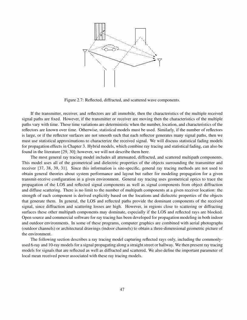
Figure 2.7: Reflected, diffracted, and scattered wave components.

If the transmitter, receiver, and reflectors are all immobile, then the characteristics of the multiple received

signal paths are fixed. However, if the transmitter or receiver are moving then the characteristics of the multiple

paths vary with time. These time variations are deterministic when the number, location, and characteristics of the

reflectors are known over time. Otherwise, statistical models must be used. Similarly, if the number of reflectors

is large, or if the reflector surfaces are not smooth such that each reflector generates many signal paths, then we

must use statistical approximations to characterize the received signal. We will discuss statistical fading models

for propagation effects in Chapter 3. Hybrid models, which combine ray tracing and statistical fading, can also be

found in the literature [29, 30]; however, we will not describe them here.

The most general ray tracing model includes all attenuated, diffracted, and scattered multipath components.

This model uses all of the geometrical and dielectric properties of the objects surrounding the transmitter and

receiver [37, 38, 39, 31]. Since this information is site-specific, general ray tracing methods are not used to

obtain general theories about system performance and layout but rather for modeling propagation for a given

transmit-receive configuration in a given environment. General ray tracing uses geometrical optics to trace the

propagation of the LOS and reflected signal components as well as signal components from object diffraction

and diffuse scattering. There is no limit to the number of multipath components at a given receiver location: the

strength of each component is derived explicitly based on the locations and dielectric properties of the objects

that generate them. In general, the LOS and reflected paths provide the dominant components of the received

signal, since diffraction and scattering losses are high. However, in regions close to scattering or diffracting

surfaces these other multipath components may dominate, especially if the LOS and reflected rays are blocked.

Open source and commercial software for ray tracing has been developed for propagation modeling in both indoor

and outdoor environments. In some of these programs, computer graphics are combined with aerial photographs

(outdoor channels) or architectural drawings (indoor channels) to obtain a three-dimensional geometric picture of

the environment.

The following section describes a ray tracing model capturing reflected rays only, including the commonly-

used 6-ray and 10-ray models for a signal propagating along a straight street or hallway. We then present ray tracing

models for signals that are reflected as well as diffracted and scattered. We also define the important parameter of

local mean received power associated with these ray tracing models.

47

2.8.1 Multi-Ray Reflections

Most wireless channels have more than just the single reflected ray captured in the two-ray model described in

Section 2.4. The multi-ray reflection model, developed in [25, 26], is a generalization of the two-ray model based

on a propagation environment called a dielectric “canyon.” This model captures all rays that experience one or

more reflections on the path between the transmitter and receiver up to a certain maximum number of reflections.

In an outdoor setting, a dielectric canyon approximates propagation in a city with rectilinear streets6 with

buildings along both sides of the street as well as transmitter and receiver antenna heights that are close to street

level. Theoretically, an infinite number of rays can be reflected off the building fronts to arrive at the receiver;

in addition, rays may also be back-reflected from buildings behind the transmitter or receiver. However, since

some of the signal energy is dissipated with each reflection, signal paths corresponding to more than two or three

reflections can generally be ignored. When the street layout is relatively straight, back reflections are usually

negligible also. Experimental data show that the dielectric canyon model of ten rays closely approximates signal

propagation through cities with a rectilinear street layout [26]. The ten-ray model incorporates the LoS path as well

as all nine paths with one, two, or three reflections: specifically, there is the ground-reflected, single-wall reflected,

double-wall reflected, triple-wall reflected, wall-ground reflected, and ground-wall reflected paths. There are two

of each type of wall-reflected path, one for each side of the street. An overhead view of the ten-ray model is shown

in Figure 2.8. A simpler model, the six-ray model, includes a subset of these ten rays: the LOS, ground reflection,

two single-wall reflections, and two double-wall reflections.

Figure 2.8: Overhead view of the ten-ray model. Includes the line-of-sight (LOS), ground-reflected (GR), two

single-wall (SW ) reflected, two double-wall (DW ) reflected, two triple-wall (TW ) reflected, wall-ground (WG)

reflected, and ground-wall (GW ) reflected rays

For the ten-ray model, the received signal is given by

r10-ray(t) = Re

{

λ

4π

[

9∑

i=0

Ri√Giu(t− τi)e

−j2πdi/λ

di

]

ej2πfct

}

, (2.50)

where di denotes the total distance traveled the ith ray, τi = di/c, and Gi is the product of the transmit and receive

antenna power gains corresponding to the ith ray. The first two terms in the summation of (2.50) correspond to the

LoS and ground reflected path in the two-ray model (2.12), hence R0 = 1 since there is no reflection of the LoS

path. For the ith reflection path, i > 0, the coefficient Ri is either a single reflection coefficient given by (2.16)

or, if the path corresponds to multiple reflections, the product of the reflection coefficients corresponding to each

reflection. The dielectric constants used in (2.50) are approximately the same as the ground dielectric, so εr = 15 is

used for all the calculations of Ri. The delay spread of the 10-ray and 6-ray models equals the difference between

the delay of the LOS ray and that of the reflected ray with the largest delay: maxi τi − τ0.

6A rectilinear city is flat and has linear streets that intersect at 90◦ angles, as in midtown Manhattan.

48

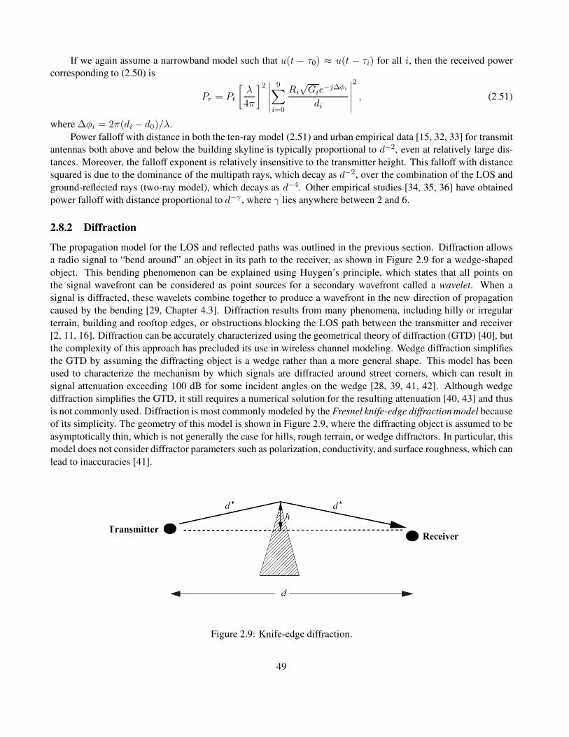
If we again assume a narrowband model such that u(t − τ0) ≈ u(t − τi) for all i, then the received power

corresponding to (2.50) is

Pr = Pt

[

λ

4π

]2∣

∣

∣

∣

∣

9∑

i=0

Ri√Gie

−j∆φi

di

∣

∣

∣

∣

∣

2

, (2.51)

where ∆φi = 2π(di − d0)/λ.

Power falloff with distance in both the ten-ray model (2.51) and urban empirical data [15, 32, 33] for transmit

antennas both above and below the building skyline is typically proportional to d−2, even at relatively large dis-

tances. Moreover, the falloff exponent is relatively insensitive to the transmitter height. This falloff with distance

squared is due to the dominance of the multipath rays, which decay as d−2, over the combination of the LOS and

ground-reflected rays (two-ray model), which decays as d−4. Other empirical studies [34, 35, 36] have obtained

power falloff with distance proportional to d−γ , where γ lies anywhere between 2 and 6.

2.8.2 Diffraction

The propagation model for the LOS and reflected paths was outlined in the previous section. Diffraction allows

a radio signal to “bend around” an object in its path to the receiver, as shown in Figure 2.9 for a wedge-shaped

object. This bending phenomenon can be explained using Huygen’s principle, which states that all points on

the signal wavefront can be considered as point sources for a secondary wavefront called a wavelet. When a

signal is diffracted, these wavelets combine together to produce a wavefront in the new direction of propagation

caused by the bending [29, Chapter 4.3]. Diffraction results from many phenomena, including hilly or irregular

terrain, building and rooftop edges, or obstructions blocking the LOS path between the transmitter and receiver

[2, 11, 16]. Diffraction can be accurately characterized using the geometrical theory of diffraction (GTD) [40], but

the complexity of this approach has precluded its use in wireless channel modeling. Wedge diffraction simplifies

the GTD by assuming the diffracting object is a wedge rather than a more general shape. This model has been

used to characterize the mechanism by which signals are diffracted around street corners, which can result in

signal attenuation exceeding 100 dB for some incident angles on the wedge [28, 39, 41, 42]. Although wedge

diffraction simplifies the GTD, it still requires a numerical solution for the resulting attenuation [40, 43] and thus

is not commonly used. Diffraction is most commonly modeled by the Fresnel knife-edge diffraction model because

of its simplicity. The geometry of this model is shown in Figure 2.9, where the diffracting object is assumed to be

asymptotically thin, which is not generally the case for hills, rough terrain, or wedge diffractors. In particular, this

model does not consider diffractor parameters such as polarization, conductivity, and surface roughness, which can

lead to inaccuracies [41].

Figure 2.9: Knife-edge diffraction.

49

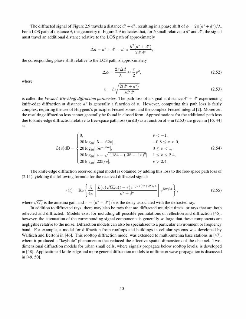
The diffracted signal of Figure 2.9 travels a distance d∗ +d?, resulting in a phase shift of φ = 2π(d∗+d?)/λ.

For a LOS path of distance d, the geometry of Figure 2.9 indicates that, for h small relative to d∗ and d?, the signal

must travel an additional distance relative to the LOS path of approximately

∆d = d∗ + d? − d ≈ h2(d∗ + d?)

2d∗d?;

the corresponding phase shift relative to the LOS path is approximately

∆φ =2π∆d

λ≈ π

2v2, (2.52)

where

v = h

√

2(d∗ + d?)

λd∗d?(2.53)

is called the Fresnel–Kirchhoff diffraction parameter. The path loss of a signal at distance d∗ + d? experiencing

knife-edge diffraction at distance d∗ is generally a function of v. However, computing this path loss is fairly

complex, requiring the use of Huygens’s principle, Fresnel zones, and the complex Fresnel integral [2]. Moreover,

the resulting diffraction loss cannot generally be found in closed form. Approximations for the additional path loss

due to knife-edge diffraction relative to free-space path loss (in dB) as a function of v in (2.53) are given in [16, 44]

as

L(v)dB =

0, v < −1,

20 log10[.5− .62v], −0.8 ≤ v < 0,

20 log10[.5e−.95v], 0 ≤ v < 1,

20 log10[.4−√

.1184− (.38− .1v)2], 1 ≤ v ≤ 2.4,

20 log10[.225/v], v > 2.4.

(2.54)

The knife-edge diffraction received signal model is obtained by adding this loss to the free-space path loss of

(2.11), yielding the following formula for the received diffracted signal:

r(t) = Re

{

λ

4π

[

L(v)√Gdu(t− τ)e−j2π(d∗+d?)/λ

d∗ + d?

]

ej2πfct

}

, (2.55)

where√Gd is the antenna gain and τ = (d∗ + d?)/c is the delay associated with the defracted ray.

In addition to diffracted rays, there may also be rays that are diffracted multiple times, or rays that are both

reflected and diffracted. Models exist for including all possible permutations of reflection and diffraction [45];

however, the attenuation of the corresponding signal components is generally so large that these components are

negligible relative to the noise. Diffraction models can also be specialized to a particular environment or frequency

band. For example, a model for diffraction from rooftops and buildings in cellular systems was developed by

Walfisch and Bertoni in [46]. This rooftop diffraction model was extended to multi-antenna base stations in [47],

where it produced a “keyhole” phenomenon that reduced the effective spatial dimensions of the channel. Two-

dimensional diffraction models for urban small cells, where signals propagate below rooftop levels, is developed

in [48]. Application of knife-edge and more general diffraction models to millimeter wave propagation is discussed

in [49, 50].

50

Figure 2.10: Scattering.

2.8.3 Scattering

A scattered ray, shown in Figure 2.10 by the segments sα and sβ, has a path loss proportional to the product of

sα and sβ . This multiplicative dependence is due to the additional spreading loss that the ray experiences after

scattering. The received signal due to a scattered ray is given by the bistatic radar equation [51]:

r(t) = Re

{

λ

4π

[√Gsσu(t− τ)e−j2π(s∗+s?)/λ

√4πs∗s?

]

ej2πfct

}

, (2.56)

where τ = (s∗ +s?)/c is the delay associated with the scattered ray; σ (in square meters) is the radar cross-section

of the scattering object, which depends on the roughness, size, and shape of the scatterer; and Gs is the antenna

power gain. The model assumes that the signal propagates from the transmitter to the scatterer based on free-space

propagation and is then re-radiated by the scatterer with transmit power equal to σ times the received power at the

scatterer. From (2.56), the path loss associated with scattering is

Pr dBm = Pt dBm + 10 log10(Gs) + 20 log10(λ) + 10 log10(σ)

−30 log(4π)− 20 log10(s∗) − 20 log10(s

?). (2.57)

Empirical values of 10 log10 σ were determined in [52] for different buildings in several cities. Results from this

study indicate that 10 log10 σ in dBm2 ranges from −4.5 dBm2 to 55.7 dBm2, where dBm2 denotes the dB value

of the σ measurement with respect to one square meter.

2.8.4 Multipath Model with Reflection, Diffraction, and Scattering

The received signal is determined from the superposition of all the components due to the multiple rays. Thus, if

we have a LOS ray, Nr reflected rays, Nd diffracted rays, and Ns scattered rays, the total received signal is

51

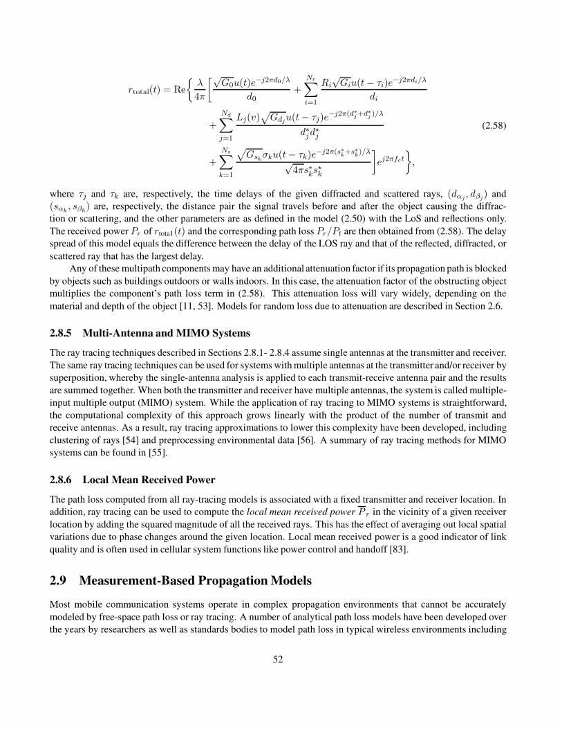
rtotal(t) = Re

{

λ

4π

[√G0u(t)e

−j2πd0/λ

d0+

Nr∑

i=1

Ri√Giu(t− τi)e

−j2πdi/λ

di

+

Nd∑

j=1

Lj(v)√

Gdju(t− τj)e

−j2π(d∗j +d?j )/λ

d∗jd?j

+

Ns∑

k=1

√

Gskσku(t− τk)e−j2π(s∗

k+s?

k)/λ

√4πs∗ks

?k

]

ej2πfct

}

,

(2.58)

where τj and τk are, respectively, the time delays of the given diffracted and scattered rays, (dαj, dβj

) and

(sαk, sβk

) are, respectively, the distance pair the signal travels before and after the object causing the diffrac-

tion or scattering, and the other parameters are as defined in the model (2.50) with the LoS and reflections only.

The received power Pr of rtota1(t) and the corresponding path loss Pr/Pt are then obtained from (2.58). The delay

spread of this model equals the difference between the delay of the LOS ray and that of the reflected, diffracted, or

scattered ray that has the largest delay.

Any of these multipath components may have an additional attenuation factor if its propagation path is blocked

by objects such as buildings outdoors or walls indoors. In this case, the attenuation factor of the obstructing object

multiplies the component’s path loss term in (2.58). This attenuation loss will vary widely, depending on the

material and depth of the object [11, 53]. Models for random loss due to attenuation are described in Section 2.6.

2.8.5 Multi-Antenna and MIMO Systems

The ray tracing techniques described in Sections 2.8.1- 2.8.4 assume single antennas at the transmitter and receiver.

The same ray tracing techniques can be used for systems with multiple antennas at the transmitter and/or receiver by

superposition, whereby the single-antenna analysis is applied to each transmit-receive antenna pair and the results

are summed together. When both the transmitter and receiver have multiple antennas, the system is called multiple-

input multiple output (MIMO) system. While the application of ray tracing to MIMO systems is straightforward,

the computational complexity of this approach grows linearly with the product of the number of transmit and

receive antennas. As a result, ray tracing approximations to lower this complexity have been developed, including

clustering of rays [54] and preprocessing environmental data [56]. A summary of ray tracing methods for MIMO

systems can be found in [55].

2.8.6 Local Mean Received Power

The path loss computed from all ray-tracing models is associated with a fixed transmitter and receiver location. In

addition, ray tracing can be used to compute the local mean received power P r in the vicinity of a given receiver

location by adding the squared magnitude of all the received rays. This has the effect of averaging out local spatial

variations due to phase changes around the given location. Local mean received power is a good indicator of link

quality and is often used in cellular system functions like power control and handoff [83].

2.9 Measurement-Based Propagation Models

Most mobile communication systems operate in complex propagation environments that cannot be accurately

modeled by free-space path loss or ray tracing. A number of analytical path loss models have been developed over

the years by researchers as well as standards bodies to model path loss in typical wireless environments including

52

urban macrocells and small cells, suburban areas, rural areas, and inside buildings with different characteristics

[11, 57, 59, 74, 17]. These models are generally based on large empirical measurement campaigns that can range

over a variety of distances, frequency ranges, geographical regions for outdoor models, and building types for

indoor models. These analytical models have the highest accuracy when they are applied to propagation conditions

similar to those under which the empirical measurements that the models are based on were made. In this section

we describe the most common analytical path loss models based on empirical measurements for both indoor and

outdoor systems.

Analytical models characterize Pr/Pt as a function of distance, so path loss is well-defined. In contrast,

empirical measurements of Pr/Pt as a function of distance include the effects of path loss, shadowing, multipath,

and other site-specific factors that affect propagation. In order to remove multipath effects, empirical measurements

for path loss typically average their received power measurements and the corresponding path loss at a given

distance over several wavelengths. This average path loss is called the local mean attenuation (LMA) at distance

d, and it generally decreases with d owing to free-space path loss and signal obstructions. The LMA in a given

environment, such as a city, depends on the specific location of the transmitter and receiver corresponding to

the LMA measurement. To characterize LMA more generally, measurements are typically taken throughout the

environment and possibly in multiple environments with similar characteristics. Thus, the empirical path loss

PL(d) for a given environment (a city, suburban area, or office building) is defined as the average of the LMA

measurements at distance d averaged over all available measurements in the given environment. For example,

empirical path loss for a generic downtown area with a rectangular street grid might be obtained by averaging

LMA measurements in New York City, downtown San Francisco, and downtown Chicago. The empirical path loss

models given in this section are all obtained from average LMA measurements. Empirical path loss models can

also be developed or refined using measurement-driven learning applied to continuous LMA data collection [75].

2.9.1 Okumura Model

One of the most well-known models for signal prediction in large urban macrocells is the Okumura model [84].

This model is applicable over distances of 1–100 km and frequency ranges of 150–1500 MHz. Okumura used

extensive measurements of base station-to-mobile signal attenuation throughout Tokyo to develop a set of curves

giving median attenuation relative to free space of signal propagation in irregular terrain. The base station heights

for these measurements were 30–100 m, a range whose upper end is higher than typical base stations today. The

empirical path loss formula of Okumura at distance d parameterized by the carrier frequency fc is given by

PL(d) dB = L(fc, d) +Aµ(fc, d)−G(ht) −G(hr) −GAREA, (2.59)

where L(fc, d) is free-space path loss at distance d and carrier frequency fc, Aµ(fc, d) is the median attenuation in

addition to free-space path loss across all environments,G(ht) is the base station antenna height gain factor, G(hr)is the mobile antenna height gain factor, and GAREA is the gain due to the type of environment. The values of

Aµ(fc, d) and GAREA are obtained from Okumura’s empirical plots [84, 11]. Okumura derived empirical formulas

for G(ht) and G(hr) as follows:

G(ht) = 20 log10(ht/200), 30 m < ht < 1000 m; (2.60)

G(hr) =

{

10 log10(hr/3), hr ≤ 3 m,

20 log10(hr/3), 3 m < hr < 10 m.(2.61)

Correction factors related to terrain are also developed in [84] that improve the model’s accuracy. Okumura’s

model has a 10–14 dB empirical standard deviation between the path loss predicted by the model and the path loss

53

associated with one of the measurements used to develop the model. The expected error in using Okumura’s model

for environments not based on these measurements is generally higher.

2.9.2 Hata Model

The Hata model [85] is an empirical formulation of the graphical path loss data provided by Okumura and is valid

over roughly the same range of frequencies, 150–1500 MHz. This empirical model simplifies calculation of path

loss because it is a closed-form formula and is not based on empirical curves for the different parameters. The

standard formula for empirical path loss in urban areas under the Hata model is

PL,urban(d) dB = 69.55 + 26.16 log10(fc) − 13.82 log10(ht) − a(hr)

+ (44.9− 6.55 log10(ht)) log10(d). (2.62)

The parameters in this model are the same as under the Okumura model, and a(hr) is a correction factor for the

mobile antenna height based on the size of the coverage area [85, 11]. For small to medium-sized cities, this factor

is given by

a(hr) = (1.1 log10(fc) − .7)hr − (1.56 log10(fc)− .8) dB,

and for larger cities at frequencies fc > 300 MHz by

a(hr) = 3.2(log10(11.75hr))2 − 4.97 dB.

Corrections to the urban model are made for suburban and rural propagation, so that these models are (respec-

tively)

PL,suburban(d) dB = PL,urban(d) dB − 2[log10(fc/28)]2 − 5.4 (2.63)

and

PL,rural(d) dB = PL,urban(d) dB − 4.78[log10(fc)]2 + 18.33 log10(fc) −K, (2.64)

where K ranges from 35.94 (countryside) to 40.94 (desert). Unlike the Okumura model, the Hata model does

not provide for any path-specific correction factors. The Hata model well approximates the Okumura model for

distances d > 1 km. Hence it is a good model for early-generation cellular systems operating in cities, but it

does not model propagation well in cellular systems with smaller cell sizes, multiple antennas, or higher frequen-

cies. Indoor environments are also not captured by the Hata model. As cellular systems evolved beyond their

early deployments, research into more complex propagation models was undertaken by multiple organizations, as

described in the next section.

2.9.3 Cellular System Models

Following the success of early cellular systems, funding agencies and standards bodies worldwide launched

projects to develop standardized cellular system channel models for the environments, carrier frequencies, cell

sizes, and multiple antenna characteristics of these evolving systems. These standardized channel models can be

used to evaluate different candidate cellular technologies in a uniform manner, and also provide guidelines for

expected system performance in typical environments and operating conditions. Cellular system channel models

span frequency ranges from .5 GHz to 100 GHz, indoor and outdoor environments with both LOS and non-LOS

propagation, small and large cells sizes, and multiple antenna transmitters and receiver of different antenna heights,

54

elevation angles, and polarizations. Models for all of these scenarios have been developed by 3GPP and the ITU

[57, 58], whereas other standardized models are applicable to a subset of these settings. To illustrate some basic

properties of these standardized models, in this section we provide the LOS path loss formulas for a few stan-

dardized models, which follow either the single-slope or dual-slope formulas ( (2.23) and (2.27), respectively)

with model-specific constants. Extensions of these models to more complex environments is also discussed. More

details on the unique characteristics of millimeter wave propagation are provided in Section 2.9.5.

An early project to standardize channel models for cellular systems was undertaken by the European coop-

erative for scientific and technical research (COST). The COST 207 program, launched in 1984, brought together

industry, government, and academia under a common umbrella to develop common propagation models for the

emerging 2G cellular systems. The subsequent COST 231 project was focused on extending earlier channel mod-

els to carrier frequencies up to 2 GHz. The resulting model, referred to as the COST 231 extension to the Hata

model [86], has the following path loss expression:

PL, urban(d) dB = 46.3 + 33.9 log10(fc) − 13.82 log10(ht) − a(hr)

+ (44.9− 6.55 log10(ht)) log10(d) +CM , (2.65)

where a(hr) is the same correction factor as in the Hata model and CM = 0 dB for medium-sized cities and

suburbs while CM = 3 dB for metropolitan areas. The COST 231 extension to the Hata model is restricted to

the following range of parameters: 1.5 GHz < fc < 2 GHz, 30 m < ht < 200 m, 1 m < hr < 10 m, and

1 km < d < 20 km. Given the Okumura measurements on which it is based, this model is most accurate for

heterogeneous macrocell-only cellular system architectures with single-antenna base stations and terminals. The

COST 231 model was further extended to incorporate new features and environments of the evolving cellular

systems and standards, including diffraction and non-LOS propagation (COST-231-WI)[29], multiple base station

antennas (COST 259) [88], and multiple antennas at both the base stations and the mobile terminals (COST 273,

COST 2100) [89, 90].

The 3GPP standards body maintains a family of channel models characterizing signal propagation for the

different environments and frequencies in which their cellular systems operate [57]. These include path loss

models for both LOS and non-LOS propagation in outdoor macrocells and small cells as well as for indoor of-

fice buildings. The 3GPP outdoor propagation models follow the dual-slope path loss model (2.27); they have

a distance-dependent pathloss exponent that takes on two different values, γ1 and γ2, for distances that are, re-

spectively, smaller or greater than the breakpoint distance. The breakpoint distance is set to the critical distance

dc = 4hthr/λ given by (2.21) in the two-ray model based on the effective transmit (ht) and receive (hr) antenna

heights7. In particular, the 3GPP path loss for LOS propagation in outdoor macrocells and small cells is given by

PL(d) dB =

{

20 log10(fc) + κ+ 10γ1 log10(d), d ≤ dc,

20 log10(fc) + κ+ 10γ2 log10(d) + η log10

(

d2c + (ht − hr)

2)

, d > dc(2.66)

for d in meters and fc in GHz. The 3GPP indoor office model is governed by the first terms of (2.66) for all

distances (i.e., there is no breakpoint distance in the indoor model due to the shorter distances involved). At

distances below dc this model has three separate terms: the constant κ that captures environment and antenna

parameters independent of distance and frequency, the term 20 log10 fc that captures frequency-dependent path

loss, and the term 10γi log10(d) that captures distance-dependent path loss. The frequency-dependent path loss

20 log10 fc is the same as in free space (2.10), and this term along with κ are captured by the constant K in the

single-slope model (2.23). At distances above dc the macrocell and small cell models have a fourth term that

captures path loss dependence on antenna heights. The values of κ, γi, and η for the macrocell, small cell, and

indoor office models are given in Table 2.4.

7In the 3GPP model the effective antennas heights are the actual heights reduced by 1m.

55

Table 2.4: Parameters for 3GPP LOS Path Loss Models

Parameter Macrocell Small Cell Indoor Office

κ 28 32.4 32.4

γ γ1 = 22, γ2 = 40 γ1 = 21, γ2 = 40 γ1 = 17.3

η -9 -9.5 NA

The 3GPP family of channel models also include non-LOS propagation models that take path loss to be the

maximum of the LOS path loss model and a different non-LOS path loss model. The non-LOS path loss model

is of the same form as (2.66) but with different parameters and a fourth term that depends only on the receiver

height hr. There is also a 3GPP rural macrocell model that includes additional parameters of the environment such

as building heights and street widths. The 3GPP Spatial Channel Model (SCM) incorporates MIMO parameters.

Details can be found in [57]. The ITU channel models are similar to the 3GPP channel family and cover the same

frequency range of .5-100 GHz [58].

The European WINNER (Wireless World Initiative New Radio) I and II projects created a similar family of

channel models as 3GPP for cellular system propagation under different conditions and environments [59]. The

WINNER path loss model is similar to the single-slope model (2.23) with the constant K broken into 3 separate

terms. Specifically, the path loss in the WINNER propagation model 10 log10(Pt/Pr) is given by

PLdBm = 10γ log10(d) + κ+ β log10(.2fc) +X (2.67)

for d in meters and fc in GHz, where γ is the path loss exponent, κ is the path loss at the antenna near-field

reference distance, typically a few signal wavelengths [12], which is independent of frequency, C log10(.2fc) is

the frequency-dependence term, and X is an optional environment-specific term that may, for example, capture a

fixed attenuation at all distances. The Winner II model includes MIMO channel parameters.

The COST, 3GPP, ITU, and WINNER families of channel models are widely used by researchers and prac-

titioners for modeling path loss in cellular systems at frequencies below 6 GHz, with the 3GPP and ITU models

covering frequencies up to 100 GHz. These models also include delay spread parameters ranging from tens of

nanoseconds for indoor environments to hundreds of nanoseconds for outdoor environments. Alternative empiri-

cal channel models specifically for MIMO systems include the WIMAX 802.16 and Stanford University Interim

(SUI) channel models [76]. As cellular system architectures have evolved to include large and small cells, device-

to-device communications, base stations mounted on UAVs and drones, large antenna arrays, millimeter wave

frequencies, and very high speed mobile devices, there have been extensive measurement campaigns to charac-

terize propagation under these new configurations and conditions [77, 78, 79]. In addition, learning algorithms

that continually update channel models based on collected data have also been developed [80, 81, 82]. Clearly

measurement-based models for cellular systems will continue to evolve as new system architectures, frequency

bands, device requirements, and channel measurement tools are introduced.

2.9.4 Wi-Fi Channel Models

Prior to 802.11n, performance evaluation of 802.11 WLAN systems was done using channel models for 2.4 GHz

(802.11g) and 5 GHz (802.11a) that had been developed by individual researchers or companies. There was no

general consensus on which models to use for performance evaluation of these earlier systems. To address this

shortcoming, the 802.11n task group (TG) was formed to develop a standard set of models, called the TGn models,

to evaluate 802.11n systems. As per the specifications of the 802.11n standard, these models include both 20 MHz

and 40 MHz channels with up to 4 antennas at the transmitter and receiver. Six different TGn channel models

(models A-F) comprise the TGn family to characterize propagation in different size homes and offices as well

56

as outdoors. All six follow the dual-slope path loss model (2.27) with a path loss exponent γ1 = 2 prior to the

breakpoint distance dBP and γ2 = 3.5 above this distance. The breakpoint distance dBP = 5 m in models A, B,

and C, which correspond to LOS only, small home, and large home, respectively. This distance ranges from 10-30

m in models D-F (corresponding to small office, large office, and outdoors, respectively). The delay spread of the

multipath, normalized with respect to the LOS path, becomes the difference between the delay of the multipath

component with the largest delay and the LOS path. In these models this normalized delay spread ranges from 0ns for the A model to 150 ns for the F model. Multipath reflections are assumed to arrive in clusters based on the

indoor propagation model developed in [60]. Antenna correlation is modeled using the Kronecker model described

in [61]. Shadow fading follows the log-normal model with standard deviation σψdB= 3 for distances d < dBP.

For d > dBP, σψdB= 4 for Models A and B, σψdB

= 5 for Models C and D, and σψdB= 6 for Models E and F.

More details on the TGn models can be found in [62].

The TGac family of channels extends the TGn model to support performance evaluation of 802.11ac sys-

tems. This model increases the number of transmit and receive antennas using the same correlation model as TGn,

increases channel bandwidth up to 160 MHz, and modifies the multipath clustering models to account for simulta-

neous transmission to multiple users (multiuser MIMO). The TGax family of channel models provides additional

environmental scenarios for dense deployments both indoors and outdoors. Details of these extensions can be

found in [63, 64].

2.9.5 Millimeter Wave Models

The millimeter (mmW) frequency band, spanning the 30-300 GHz range, was not used in the first few generations

of Wi-Fi and cellular systems due to its high path loss as well as the high cost and poor performance of mmW

hardware. However, as demand for increased data rates in wireless systems continued unabated with each new

generation, utilizing the large amount of available spectrum in this band grew increasingly appealing. Moreover,

in 2005 the FCC in the US created more flexible rules for spectrum allocation in the lower part of this band to

increase its use [65]. Following this ruling, a few commercial mmW communication systems were developed for

in-home use, but the technology was not yet competitive with Wi-Fi. Interest in utilizing mmW wave spectrum

for cellular communications also started to grow, leading to outdoor channel measurement campaigns as well as

cellular system designs to overcome the propagation challenges at these high frequencies. This section provides

an overview of mmW propagation characteristics.

Since path loss is inversely proportional to frequency squared in the free space path loss formula (2.6), this

loss is much higher at mmW frequencies than at lower frequencies. However, this large free-space path loss can be

compensated by high gains associated with directional or multiple antenna technologies. In addition to free-space

path loss, signal propagation in the mmW band experiences significant attenuation at specific carrier frequencies

due to interactions with oxygen, water, and other molecular components in the air. Attenuation due to shadowing

from objects and people is more severe at these frequencies and shadowing can also cause scattering of directed

beams. As a result, there is typically only a small number of multipath components in mmWave channels whose

received power is above the noise floor.

The resonant frequency of oxygen (O2) molecules leads to heavy absorption, up to 15 dB/km, for signals

transmitted through the air at carrier frequencies around 60 GHz. There is also significant absorption due to the

resonant frequencies of O2 or water vapor (H2O) at 119, 183, and 325 GHz, with a small peak at 24 GHz. The

combined effects of free-space path loss and the O2 and H2O absorption in non-rainy conditions is illustrated in

Fig. 2.11 from [67]. It can be seen from this figure that atmospheric absorption is somewhat larger at sea level than

at higher altitudes due to increased water vapor concentration.

Millimeter wave propagation is also affected by rain absorption. In particular, rain causes scattering since the

wavelength of a mmW signal is roughly the same size as a raindrop. The higher the rain rate, the more scattering

occurs and hence the higher the absorption. A model for attenuation at different rain rates for mmW propagation

57

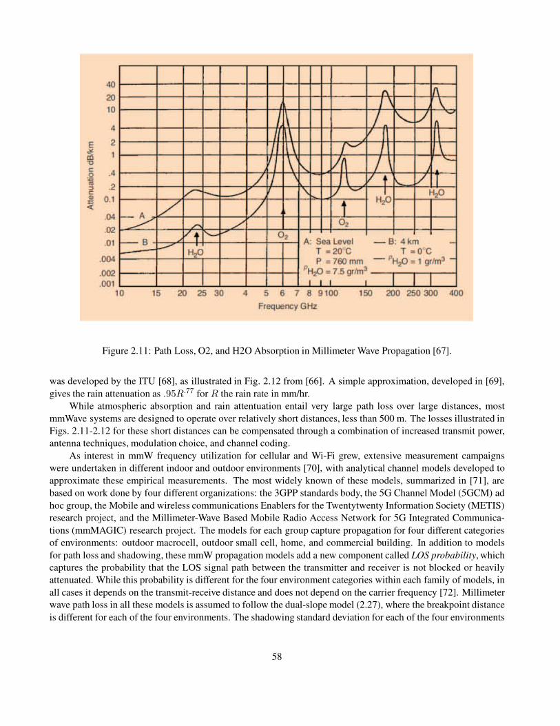
Figure 2.11: Path Loss, O2, and H2O Absorption in Millimeter Wave Propagation [67].

was developed by the ITU [68], as illustrated in Fig. 2.12 from [66]. A simple approximation, developed in [69],

gives the rain attenuation as .95R.77 for R the rain rate in mm/hr.

While atmospheric absorption and rain attentuation entail very large path loss over large distances, most

mmWave systems are designed to operate over relatively short distances, less than 500 m. The losses illustrated in

Figs. 2.11-2.12 for these short distances can be compensated through a combination of increased transmit power,

antenna techniques, modulation choice, and channel coding.

As interest in mmW frequency utilization for cellular and Wi-Fi grew, extensive measurement campaigns

were undertaken in different indoor and outdoor environments [70], with analytical channel models developed to

approximate these empirical measurements. The most widely known of these models, summarized in [71], are

based on work done by four different organizations: the 3GPP standards body, the 5G Channel Model (5GCM) ad

hoc group, the Mobile and wireless communications Enablers for the Twentytwenty Information Society (METIS)

research project, and the Millimeter-Wave Based Mobile Radio Access Network for 5G Integrated Communica-

tions (mmMAGIC) research project. The models for each group capture propagation for four different categories

of environments: outdoor macrocell, outdoor small cell, home, and commercial building. In addition to models

for path loss and shadowing, these mmW propagation models add a new component called LOS probability, which

captures the probability that the LOS signal path between the transmitter and receiver is not blocked or heavily

attenuated. While this probability is different for the four environment categories within each family of models, in

all cases it depends on the transmit-receive distance and does not depend on the carrier frequency [72]. Millimeter

wave path loss in all these models is assumed to follow the dual-slope model (2.27), where the breakpoint distance

is different for each of the four environments. The shadowing standard deviation for each of the four environments

58

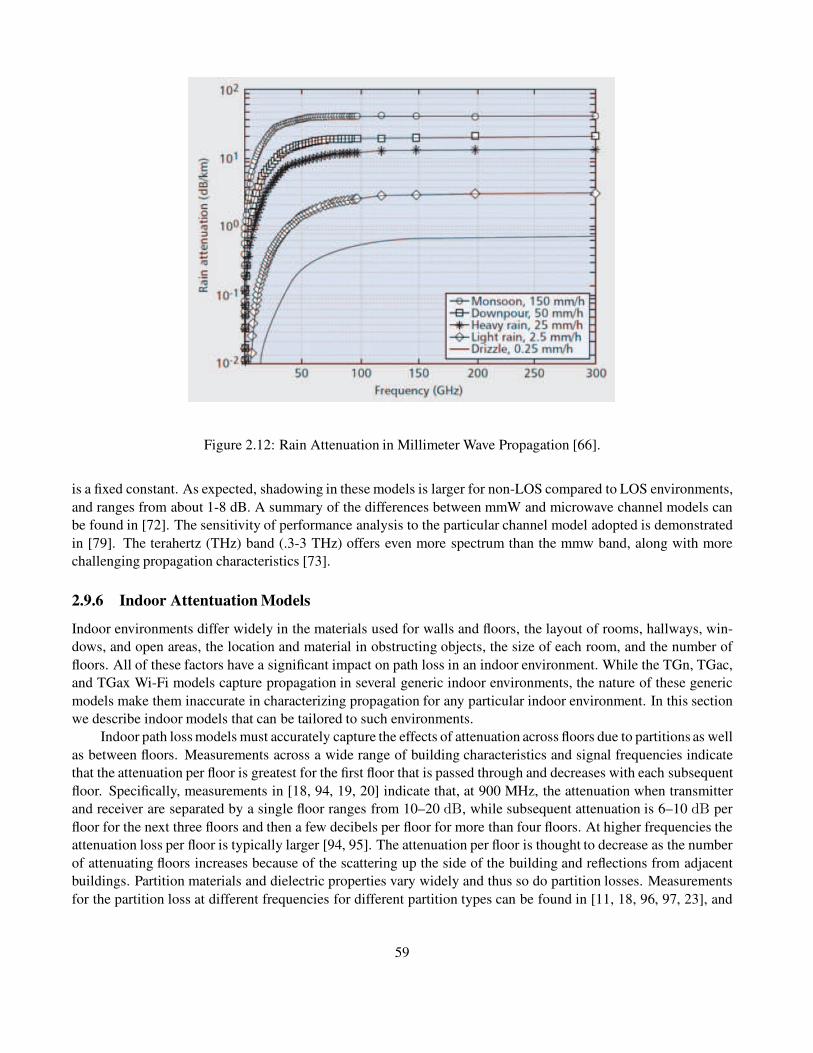
Figure 2.12: Rain Attenuation in Millimeter Wave Propagation [66].

is a fixed constant. As expected, shadowing in these models is larger for non-LOS compared to LOS environments,

and ranges from about 1-8 dB. A summary of the differences between mmW and microwave channel models can

be found in [72]. The sensitivity of performance analysis to the particular channel model adopted is demonstrated

in [79]. The terahertz (THz) band (.3-3 THz) offers even more spectrum than the mmw band, along with more

challenging propagation characteristics [73].

2.9.6 Indoor Attentuation Models

Indoor environments differ widely in the materials used for walls and floors, the layout of rooms, hallways, win-

dows, and open areas, the location and material in obstructing objects, the size of each room, and the number of

floors. All of these factors have a significant impact on path loss in an indoor environment. While the TGn, TGac,

and TGax Wi-Fi models capture propagation in several generic indoor environments, the nature of these generic

models make them inaccurate in characterizing propagation for any particular indoor environment. In this section

we describe indoor models that can be tailored to such environments.

Indoor path loss models must accurately capture the effects of attenuation across floors due to partitions as well

as between floors. Measurements across a wide range of building characteristics and signal frequencies indicate

that the attenuation per floor is greatest for the first floor that is passed through and decreases with each subsequent

floor. Specifically, measurements in [18, 94, 19, 20] indicate that, at 900 MHz, the attenuation when transmitter

and receiver are separated by a single floor ranges from 10–20 dB, while subsequent attenuation is 6–10 dB per

floor for the next three floors and then a few decibels per floor for more than four floors. At higher frequencies the

attenuation loss per floor is typically larger [94, 95]. The attenuation per floor is thought to decrease as the number

of attenuating floors increases because of the scattering up the side of the building and reflections from adjacent

buildings. Partition materials and dielectric properties vary widely and thus so do partition losses. Measurements

for the partition loss at different frequencies for different partition types can be found in [11, 18, 96, 97, 23], and

59

Table 2.5: Typical partition losses at fc ≈ 1 GHz

Partition type Partition loss (dB)

Cloth partition 1.4

Double plasterboard wall 3.4

Foil insulation 3.9

Concrete wall 13

Aluminum siding 20.4

All metal 26

Table 2.6: ITU penetration loss model

Material Penetration loss (dB)

Standard multi-pane glass 2 + 0.2fcInfrared reflective glass 23 + .3fc

Concrete 5 + 4fcWood 4.85 + 0.12fc

Table 2.5 indicates a few examples of partition losses measured at around 1 GHz from this data. The partition

loss obtained by different researchers for the same partition type at the same frequency often varies widely, so it is

difficult to make generalizations about partition loss from a specific data set.

The experimental data for floor and partition loss can be added to an analytical or empirical dB path loss

model PL(d) as

Pr dBm = Pt dBm − PL(d)−Nf∑

i=1

FAFi −Np∑

i=1

PAFi, (2.68)

where FAFi represents the floor attenuation factor for the ith floor traversed by the signal and PAFi represents

the partition attenuation factor associated with the ith partition traversed by the signal. The number of floors and

partitions traversed by the signal are Nf and Np, respectively.

Another important factor for indoor systems whose transmitter is located outside the building is outdoor-to-

indoor penetration loss. Measurements indicate that this penetration loss is a function of frequency, height, and

the exterior wall or window material. For carrier frequencies from .9-3 GHz penetration loss measurements range

from 8 dB to 20 dB [2, 21, 100, 101]. Penetration loss for mmWave signals generally increases with frequency.

Hence, the 3GPP, ITU, 5GCM, and mmMAGIC propagation models include a component for outdoor-to-indoor

penetration loss as a function of both frequency and the exterior wall or window material [57, ?, 70]. The ITU

penetration loss model as a function of frequency fc and for different wall and window materials is given in

Table 2.6. In general penetration loss decreases by about 1.4 dB per floor at floors above the ground floor. This

decrease is due to reduced clutter at higher floors and the higher likelihood of a LOS path.

60

Chapter 2 Problems

1. Under the free-space path loss model, find the transmit power required to obtain a received power of 1 dBm

for a wireless system with isotropic antennas (Gt = Gr = 1) and a carrier frequency fc = 5 GHz, assuming

a distance d = 10 m. Repeat for d = 100 m.

2. For the two-ray model with transmitter–receiver separation d = 100 m, ht = 10 m, and hr = 2 m, find the

delay spread between the two signals.

3. For the two-ray model, show how a Taylor series approximation applied to (2.14) results in the approximation

∆φ =2π(d1 − d0)

λ≈ 4πhthr

λd.

4. For the two-ray model, derive an approximate expression for the distance values below the critical distance

dc at which signal nulls occur.

5. Find the critical distance dc under the two-ray model for a large macrocell in a suburban area with the base

station mounted on a tower or building (ht = 20 m), the receivers at height hr = 3 m, and fc = 2 GHz. Is

this a good size for cell radius in a suburban macrocell? Why or why not?

6. Suppose that, instead of a ground reflection, a two-ray model consists of a LOS component and a signal

reflected off a building to the left (or right) of the LOS path. Where must the building be located relative to

the transmitter and receiver for this model to be the same as the two-ray model with a LOS component and

ground reflection?

7. Consider a two-ray channel with impulse response h(t) = α1δ(t) + α2δ(t − .022 µs), so for input signal

s(t) to the channel, the output is r(t) = h(t)∗s(t). Find the distance separating the transmitter and receiver,

as well as α1 and α2, assuming free-space path loss on each path with a reflection coefficient of −1. Assume

the transmitter and receiver are located 8 m above the ground and that the carrier frequency is 900 MHz.

8. Directional antennas are a powerful tool to reduce the effects of multipath as well as interference. In par-

ticular, directional antennas along the LOS path for the two-ray model can reduce the attenuation effect of

ground wave cancellation, as will be illustrated in this problem. Assume the reference distance dr = 1

m. Plot the dB power (10 log10 Pr) versus log distance (log10 d) for the two-ray model with parameters

fc = 900 MHz, R = −1, ht = 50 m, hr = 2 m, G0 = 1, and the following values for G1 : G1 = 1, .316, .1,

and .01 (i.e., G1 = 0, −5, −10, and− 20 dB, respectively). Each of the four plots should range in distance

from d = 1 m to d = 100 km. Also calculate and mark the critical distance dc = 4hthr/λ on each plot, and

normalize the plots to start at approximately 0 dB. Finally, show the piecewise linear model with flat power

falloff up to distance ht, falloff 10 log10(d−2) for ht < d < dc, and falloff 10 log10(d

−4) for d ≥ dc. (On the

power loss versus log distance plot, the piecewise linear curve becomes a set of three straight lines of slope

0, 2, and 4, respectively.) Note that at large distances it becomes increasingly difficult to have G1 � G0

because this requires extremely precise angular directivity in the antennas.

9. Under what conditions is the single-slope path loss model (2.22) the same as the free-space path loss model

(2.7)?

10. Consider a receiver with noise power –160 dBm within the signal bandwidth of interest. Assume a single-

slope path loss model with d0 = 1 m, K obtained from the free-space path loss formula with isotropic

antennas and fc = 1 GHz, and γ = 4. For a transmit power of Pt = 10 mW, find the maximum distance

between the transmitter and receiver such that the received signal-to-noise power ratio is 20 dB.

61

11. For the set of empirical measurements of Pr/Pt given in Table 2.2, find the path loss exponent γ and param-

eter K that minimizes the MSE between the single-slope model (2.23) in dB and the empirical dB power

measurements, assuming that dr = 1 m. This problem differs from Example 2.5.1 in that now the two

parameters γ and K are jointly optimized to minimize MSE, rather than fixing the value of K based on

free-space path loss or the measured attenuation at the reference distance dr. Find the received power at 150

m for this single-slope path loss model with transmit power of 1 mW (0 dBm) and compare with the result in

Example 2.5.1. Does the better fitting of the data through this two-dimensional optimization lead to a larger

or smaller value for this received power? Will this always be the case for any set of empirical measurements

(why or why not)?

12. Find parameters for a multi-slope model with three segments to approximate the two-ray model path loss

(2.13) over distances between 10 and 1000 meters, assuming ht = 10 m, hr = 2 m, and G0 = G1 = 1. Plot

the path loss and the piecewise linear approximation using these parameters over this distance range.

13. This problem shows how different propagation models can lead to very different SNRs (and therefore differ-

ent link performance) for a given system design. Consider a linear cellular system using frequency division,

as might operate along a highway or rural road (see Figure 2.13). Each cell is allocated a certain band of

frequencies, and these frequencies are reused in cells spaced a distance d away. Assume the system has

square cells, 2 km per side, and that all mobiles transmit at the same power P . For the following propagation

models, determine the minimum distance that the cells operating in the same frequency band must be spaced

so that uplink SNR (the ratio of the minimum received signal-to-interference or S/I power from mobiles to

the base station) is greater than 20 dB. You can ignore all interferers except those from the two nearest cells

operating at the same frequency.

Figure 2.13: Linear cellular system for Problem 2-14.

(a) Propagation for both signal and interference follow a free-space model.

(b) Propagation for both signal and interference follow the single-slope path loss model (2.22) with d0 =

100 m, K = 1, and γ = 3.

(c) Propagation for the signal follows the single-slope path loss model with d0 = 100 m, K = 1, and

γ = 2, while propagation of the interfererence follows the same model but with γ = 4.

14. Table 2.7 lists a set of empirical path loss measurements. Assume a carrier frequency fc = 2 GHz.

(a) Find the parameters of a single-slope path loss model plus log-normal shadowing that best fit this data

assuming K is calculated from free-space path loss at the reference distance dr = 1 m.

(b) Find the path loss at 2 km based on this model.

(c) Find the outage probability at a distance d assuming the received power at d due to path loss alone is

10 dB above the required power for non-outage.

62

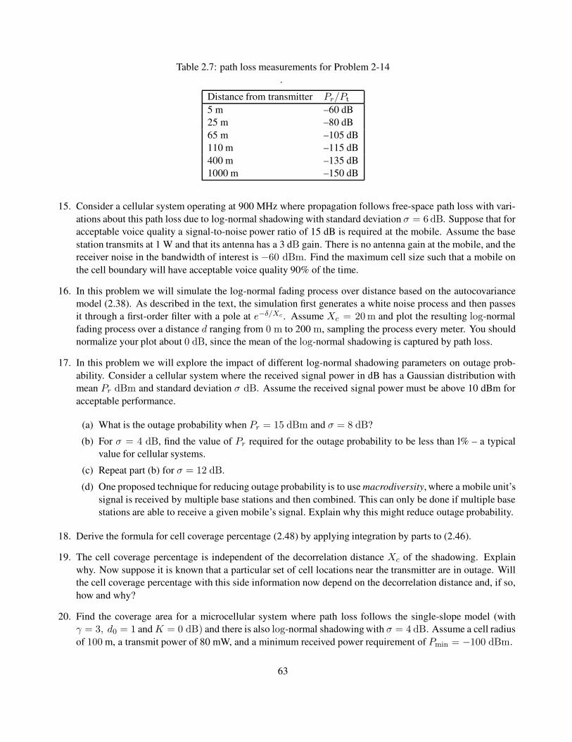
Table 2.7: path loss measurements for Problem 2-14

.

Distance from transmitter Pr/Pt

5 m –60 dB

25 m –80 dB

65 m –105 dB

110 m –115 dB

400 m –135 dB

1000 m –150 dB

15. Consider a cellular system operating at 900 MHz where propagation follows free-space path loss with vari-

ations about this path loss due to log-normal shadowing with standard deviation σ = 6 dB. Suppose that for

acceptable voice quality a signal-to-noise power ratio of 15 dB is required at the mobile. Assume the base

station transmits at 1 W and that its antenna has a 3 dB gain. There is no antenna gain at the mobile, and the

receiver noise in the bandwidth of interest is −60 dBm. Find the maximum cell size such that a mobile on

the cell boundary will have acceptable voice quality 90% of the time.

16. In this problem we will simulate the log-normal fading process over distance based on the autocovariance

model (2.38). As described in the text, the simulation first generates a white noise process and then passes

it through a first-order filter with a pole at e−δ/Xc . Assume Xc = 20 m and plot the resulting log-normal

fading process over a distance d ranging from 0 m to 200 m, sampling the process every meter. You should

normalize your plot about 0 dB, since the mean of the log-normal shadowing is captured by path loss.

17. In this problem we will explore the impact of different log-normal shadowing parameters on outage prob-

ability. Consider a cellular system where the received signal power in dB has a Gaussian distribution with

mean Pr dBm and standard deviation σ dB. Assume the received signal power must be above 10 dBm for

acceptable performance.

(a) What is the outage probability when Pr = 15 dBm and σ = 8 dB?

(b) For σ = 4 dB, find the value of Pr required for the outage probability to be less than l% – a typical

value for cellular systems.

(c) Repeat part (b) for σ = 12 dB.

(d) One proposed technique for reducing outage probability is to use macrodiversity, where a mobile unit’s

signal is received by multiple base stations and then combined. This can only be done if multiple base

stations are able to receive a given mobile’s signal. Explain why this might reduce outage probability.

18. Derive the formula for cell coverage percentage (2.48) by applying integration by parts to (2.46).

19. The cell coverage percentage is independent of the decorrelation distance Xc of the shadowing. Explain

why. Now suppose it is known that a particular set of cell locations near the transmitter are in outage. Will

the cell coverage percentage with this side information now depend on the decorrelation distance and, if so,

how and why?

20. Find the coverage area for a microcellular system where path loss follows the single-slope model (with

γ = 3, d0 = 1 and K = 0 dB) and there is also log-normal shadowing with σ = 4 dB. Assume a cell radius

of 100 m, a transmit power of 80 mW, and a minimum received power requirement of Pmin = −100 dBm.

63

21. Consider a cellular system where (a) path loss follows the single-slope model with γ = 6 and (b) there is

also log-normal shadowing with σ = 8 dB. If the received power at the cell boundary due to path loss is

20 dB higher than the minimum required received power for non-outage, find the cell coverage area.

22. In microcells, path loss exponents usually range from 2 to 6 and shadowing standard deviation typically

ranges from 4 to 12. Given a cellular system in which the received power due to path loss at the cell

boundary equals the desired level for non-outage, find the path loss and shadowing parameters within these

ranges that yield the best and worst coverage area. What is the coverage area when these parameters are in

the middle of their typical ranges?

Figure 2.14: System with scattering for Problem 2-11.

23. What average power falloff with distance do you expect for the ten-ray model if G0 = G1 >> Gi for

i = 2, ..., 9? Repeat for G0 = G1 = G2 >> Gi for i = 3, ..., 9. Explain your answers in both cases.

24. For the ten-ray model, assume that the transmitter and receiver are at the same height in the middle of a street

of width 20 m. The transmitter-receiver separation is 500 m. Find the delay spread for this model.

25. Consider a system with a transmitter, receiver, and scatterer as shown in Figure 2.14. Assume the transmitter

and receiver are both at heights ht = hr = 4 m and are separated by distance d, with the scatterer at distance

.5d along both dimensions in a two-dimensional grid of the ground – that is, on such a grid the transmitter

is located at (0, 0), the receiver at (0, d), and the scatterer at (.5d, .5d). Assume a radar cross-section of

20 dBm2, Gs = 1, and fc = 900 MHz. Find the path loss of the scattered signal for d = 1, 10, 100, and

1000 meters. Compare with the path loss at these distances if the signal is only reflected, with reflection

coefficient R = −1.

26. Find the median path loss under the Hata model assuming fc = 900 MHz, ht = 20 m, hr = 5 m, and

d = 100 m for a large urban city, a small urban city, a suburb, and a rural area. Explain qualitatively the path

loss differences for these four environments.

27. Consider a wireless link operating outdoors over 200m in the mmW freqency band. Assume the path loss

follows the single-slope model with a path loss exponent γ = 2 and reference distance for antenna far

field dr = 1 m. Without any additional attenuation caused by atmospheric and rain conditions, the model

attenuation factor K = 1. Assume rain attenuation follows the simple approximation Krain = .95R.77 for

R the rain rate in mm/hr. Assume the atmospheric absorption given in Fig. 2.11.

(a) What is the received signal power due to path loss and oxygen absorption at carrier frequencies of 60

GHz and of 80 GHz assuming a transmit power of 1W?

64

(b) Consider now only the 80 GHz link. Assume a day where it is dry at 8 am, there is a heavy drizzle of

2.5mm/Hr at 12 pm and a heavy downpour of 50mm/Hr at 5 pm. What is the required transmit power at

8 am, 12 pm and 5 pm if we desire a received signal power of -50dBm at each of these time instances?

28. Using the indoor attentuation model, determine the required transmit power for a desired received power of

–110 dBm for a signal transmitted over 100 m that goes through three floors with attenuation 15 dB, 10 dB,

and 6 dB (respectively) as well as two double plaster-board walls. Assume a reference distance dr = 1,

exponent γ = 4, and constant K = 0 dB.

65

Bibliography

[1] W. C. Jakes, Jr., Microwave Mobile Communications, Wiley, New York, 1974 [reprinted by IEEE Press].

[2] D. Parsons, The Mobile Radio Propagation Channel, 2nd Ed., Wiley, New York, 2000.

[3] M. Patzold, Mobile Fading Channels, 2nd Ed., Wiley, New York, 2011.

[4] H. L. Bertoni, Radio Propagation for Modern Wireless Systems, Prentice Hall, 1999.

[5] J. Cavers, Mobile Channel Characteristics, Springer 2000.

[6] IEEE J. Sel. Areas Commun., Special Issue on Channel and Propagation Modeling for Wireless Systems

Design, April 2002 and August 2002.

[7] N. Costa and S. Haykin, Multiple-input Multiple-output Channel Models: Theory and Practice, John Wiley

and Sons, 2010.

[8] IEEE J. Sel. Areas Commun., Special Issue on Ultra-Wideband Radio in Multiaccess Wireless Communica-

tions, December 2002.

[9] T. Rappaport, R. W. Heath Jr, R. C. Daniels, and J. N. Murdock. Millimeter Wave Wireless Communications.

Pearson Education, 2014.

[10] G. H. Spencer and M. V. R. K. Murty, “General Ray-Tracing Procedure”. Journal of the Optical Society of

America, Vol. 52, Issue 6, pp. 672-678, June 1962.

[11] T. S. Rappaport, Wireless Communications-Principles and Practice, 2nd ed., Prentice-Hall, Englewood

Cliffs, NJ, 2001.

[12] J. L. Volakis, Antenna Engineering Handbook, 4th Ed. McGraw-Hill, 2007.

[13] H. T. Friis, “A note on a simple transmission formula”, Proc. IRE, vol. 34, no. 5, pp. 254-256, May 1946.

[14] A. S. Y. Poon and R. W. Brodersen, “The role of multiple-antenna systems in emerging open access environ-

ments,” EE Times Commun. Design Conf., October 2003.

[15] A. J. Rustako, Jr., N. Amitay, G. J. Owens, and R. S. Roman, “Radio propagation at microwave frequencies

for line-of-sight microcellular mobile and personal communications,” IEEE Trans. Veh. Tech., pp. 203–10,

February 1991.

[16] W. C. Y. Lee, Mobile Communications Engineering, McGraw-Hill, New York, 1982.

66

[17] V. Erceg, L. J. Greenstein, S. Y. Tjandra, S. R. Parkoff, A. Gupta, B. Kulic, A. A. Julius, and R. Bianchi,

“An empirically based path loss model for wireless channels in suburban environments,” IEEE J. Sel. Areas

Commun., pp. 1205–11, July 1999.

[18] S. Y. Seidel and T. S. Rappaport, “914 MHz path loss prediction models for indoor wireless communications

in multifloored buildings,” IEEE Trans. Ant. Prop., pp. 207–17, February 1992.

[19] A. F. Toledo and A. M. D. Turkmani, “Propagation into and within buildings at 900, 1800, and 2300 MHz,”

Proc. IEEE Veh. Tech. Conf., pp. 633–6, May 1992.

[20] F. C. Owen and C. D. Pudney, “Radio propagation for digital cordless telephones at 1700 MHz and 900 MHz,”

Elec. Lett., pp. 52–3, September 1988.

[21] A. F. Toledo, A. M. D. Turkmani, and J. D. Parsons, “Estimating coverage of radio transmission into and

within buildings at 900, 1800, and 2300 MHz,” IEEE Pers. Commun. Mag., pp. 40–7, Apri1 1998.

[22] D. M. J. Devasirvathan, R. R. Murray, and D. R. Woiter, “Time delay spread measurements in a wireless local

loop test bed,” Proc. IEEE Veh. Tech. Conf., pp. 241–5, May 1995.

[23] G. Durgin, T. S. Rappaport, and H. Xu, “Partition-based path loss analysis for in-home and residential areas

at 5.85 GHz,” Proc. IEEE Globecom Conf., pp. 904–9, November 1998.

[24] T. Kurner, D. J. Cichon, and W. Wiesbeck, “Concepts and results for 3D digital terrain-based wave propaga-

tion models: An overview,” IEEE J. Sel. Areas Commun., pp. 1002–12, September 1993.

[25] A. J. Rustako, Jr., N. Amitay, G. J. Owens, and R.S. Roman, Radio propagation at microwave frequencies

for line-of-sight microcellular mobile and personal communications, IEEE Trans. Veh. Technol., vol. 40, pp.

203–210, February 1991.

[26] N. Amitay, “Modeling and computer simulation of wave propagation in lineal line-of-sight microcells,” IEEE

Trans. Veh. Tech., pp. 337–42, November 1992.

[27] J. W. McKown and R. L. Hamilton, Jr., “Ray tracing as a design tool for radio networks,” IEEE Network, pp.

27–30, November 1991.

[28] K. A. Remley, H. R. Anderson, and A. Weisshar, “Improving the accuracy of ray-tracing techniques for

indoor propagation modeling,” IEEE Trans. Veh. Tech., pp. 2350–8, November 2000.

[29] A. Domazetovic, L. J. Greenstein, N. Mandayan, and I. Seskar, “A new modeling approach for wireless

channels with predictable path geometries,” Proc. IEEE Veh. Tech. Conf., September 2002.

[30] J. H. Tarng, W.-S. Liu, Y.-F. Huang, and J.-M. Huang, “A novel and efficient hybrid model of radio multipath-

fading channels in indoor environments,” IEEE Trans. Ant. Prop., pp. 585–94, March 2003.

[31] Z. Yun and M. F. Iskander. “Ray tracing for radio propagation modeling: Principles and applications.” IEEE

Access Vol. 3, 2015, pp. 1089-1100.

[32] J.-F. Wagen, “Signal strength measurements at 881 MHz for urban microcells in downtown Tampa,” Proc.

IEEE Globecom Conf., pp. 1313–17, December 1991.

[33] R. J. C. Bultitude and G. K. Bedal, “Propagation characteristics on microcellular urban mobile radio channels

at 910 MHz,” IEEE J. Sel. Areas Commun., pp. 31–9, January 1989.

67

[34] J.-E. Berg, R. Bownds, and F. Lotse, “Path loss and fading models for microcells at 900 MHz,” Proc. IEEE

Veh. Tech. Conf., pp. 666–71, May 1992.

[35] J. H. Whitteker, “Measurements of path loss at 910 MHz for proposed microcell urban mobile systems,”

IEEE Trans. Veh. Tech., pp. 125–9, August 1988.

[36] H. Borjeson, C. Bergljung, and L. G. Olsson, “Outdoor microcell measurements at 1700 MHz,” Proc. IEEE

Veh. Tech. Conf., pp. 927–31, May 1992.

[37] K. Schaubach, N. J. Davis IV, and T. S. Rappaport, “A ray tracing method for predicting path loss and delay

spread in microcellular environments,” Proc. IEEE Veh. Tech. Conf., pp. 932–5, May 1992.

[38] F. Ikegami, S. Takeuchi, and S. Yoshida, “Theoretical prediction of mean field strength for urban mobile

radio,” IEEE Trans. Ant. Prop., pp. 299–302, March 1991.

[39] M. C. Lawton and J. P. McGeehan, “The application of GTD and ray launching techniques to channel mod-

eling for cordless radio systems,” Proc. IEEE Veh. Tech. Conf., pp. 125–30, May 1992.

[40] J. B. Keller, “Geometrical theory of diffraction,” J. Opt. Soc. Amer., 52, pp. 116–30, 1962.

[41] R. J. Luebbers, “Finite conductivity uniform GTD versus knife edge diffraction in prediction of propagation

path loss,” IEEE Trans. Ant. Prop., pp. 70–6, January 1984.

[42] C. Bergljung and L. G. Olsson, “Rigorous diffraction theory applied to street microcell propagation,” Proc.

IEEE Globecom Conf., pp. 1292–6, December 1991.

[43] R. G. Kouyoumjian and P. H. Pathak, “A uniform geomenical theory of diffraction for an edge in a perfectly

conducting surface,” Proc. IEEE, pp. 1448–61, November 1974.

[44] G. K. Chan, “Propagation and coverage prediction for cellular radio systems,” IEEE Trans. Veh. Tech., pp.

665–70, November 1991.

[45] K. C. Chamberlin and R. J. Luebbers, “An evaluation of Longley–Rice and GTD propagation models,” IEEE

Trans. Ant. Prop., pp. 1093–8, November 1982.

[46] J. Walfisch and H. L. Bertoni, “A theoretical model of UHF propagation in urban environments,” IEEE Trans.

Ant. Prop., pp. 1788–96, October 1988.

[47] D. Chizhik, G. J. Foschini, M. J. Gans and R. A. Valenzuela, “Keyholes, correlations, and capacities of

multielement transmit and receive antennas,” IEEE Transactions on Wireless Communications, vol. 1, no. 2,

pp. 361-368, April 2002.

[48] W. Zhang, “Fast two-dimensional diffraction modeling for site-specific propagation prediction in urban mi-

crocellular environments,” IEEE Trans. Veh. Techn., vol. 49, no. 2, pp. 428436, 2000.

[49] S. Deng, G. R. MacCartney and T. S. Rappaport, “Indoor and Outdoor 5G Diffraction Measurements and

Models at 10, 20, and 26 GHz,” 2016 IEEE Global Communications Conference (GLOBECOM), Washington,

DC, 2016, pp. 1-7.

[50] M. Jacob, S. Priebe, R. Dickhoff, T. Kleine-Ostmann, T. Schrader and T. Kurner, ”Diffraction in mm and

Sub-mm Wave Indoor Propagation Channels,” IEEE Transactions on Microwave Theory and Techniques,

vol. 60, no. 3, pp. 833-844, March 2012.

68

[51] M. I. Skolnik, Introduction to Radar Systems, 2nd ed., McGraw-Hill, New York, 1980.

[52] S. Y. Seidel, T. S. Rappaport, S. Jain, M. L. Lord, and R. Singh, “Path loss, scattering, and multipath delay

statistics in four European cities for digital cellular and microcellular radiotelephone,” IEEE Trans. Veh. Tech.,

pp. 721–30, November 1991.

[53] S. T. S. Chia, “1700 MHz urban microcells and their coverage into buildings,” Proc. IEEE Ant. Prop. Conf.,

pp. 504–11, York, U.K., Apri1 1991.

[54] T. Fugen, J. Maurer, W. Sorgel and W. Wiesbeck, “Characterization of multipath clusters with ray-tracing

in urban MIMO propagation environments at 2 GHz,” in 2005 IEEE Antennas and Propagation Society

International Symposium, Washington, DC, 2005, pp. 410-413.

[55] M. A. Jensen and J. W. Wallace, ”A review of antennas and propagation for MIMO wireless communications,”

IEEE Transactions on Antennas and Propagation, pp. 2810-2824, Nov. 2004.

[56] K. H. Ng, E. K. Tameh, A. Doufexi, M. Hunukumbure and A. R. Nix, ”Efficient multielement ray Trac-

ing with site-specific comparisons using measured MIMO channel data,” IEEE Transactions on Vehicular

Technology, pp. 1019-1032, May 2007.

[57] 3GPP, Study on channel model for frequencies from 0.5 to 100 GHz, 3rd Generation Partnership Project

(3GPP), Tech. Rep. TR 38.901, March 2017, Website: www.3gpp.org/DynaReport/38901.htm

[58] IMT, “Guidelines for evaluation of radio interface technologies for IMT-2020,” Tech Rep. ITU-R M.2412-0,

Oct. 2017, Website: www.itu.int/pub/R-REP-M.2412.

[59] P. Kyosti et al., WINNER II channel models, Eur. Commission, IST-4-027756-WINNER, Brussels, Belgium,

Tech. Rep. D1.1.2, Sep. 2007

[60] A. A. M. Saleh and R. Valenzuela, ”A Statistical Model for Indoor Multipath Propagation,” in IEEE Journal

on Selected Areas in Communications, vol. 5, no. 2, pp. 128-137, February 1987.

[61] L. Schumacher, K. I. Pedersen, and P.E. Mogensen, From antenna spacings to theoretical capacities guide-

lines for simulating MIMO systems, in Proc. PIMRC Conf., vol. 2, Sept. 2002, pp. 587-592.

[62] V. Erceg et al., TGn Channel Models. Doc. IEEE802.11-03/940r4.

[63] G. Breit et. al., “TGac Channel Model Addendum. IEEE 802.11-09/0308r12.

[64] J. Liu et. al., “IEEE 802.11ax Channel Model Document.” IEEE 802.11-14/0882r4.

[65] FCC Memorandum and Opinion Order 05-45 WTB Allocations and Service Rules for the 71-76 GHz, 81-86

GHz and 92-95 GHz Bands. Feb. 2005.

[66] Z. Pi and F. Khan, “An introduction to millimeter-wave mobile broadband systems, IEEE Commun. Mag.,

pp. 101107, June 2011.

[67] M. Marcus and B. Pattan, Millimeter wave propagation: Spectrum management implications, IEEE Mi-

crowave Mag., pp. 5462, June 2005.

[68] ITU-R P.838-3, Specific Model for Rain for Use in Prediction Methods, 2005.

69

[69] J. Ostrometzky and H. Messer, “Accumulated rainfall estimation using maximum attenuation of microwave

radio signal,” Proc. IEEE 8th Sensor Array and Multichannel Signal Processing Workshop (SAM), pp. 193-

196, June 2014.

[70] M. Xiao et al., “Millimeter Wave Communications for Future Mobile Networks,” IEEE Journal on Selected

Areas in Communications, vol. 35, no. 9, pp. 1909-1935, Sept. 2017.

[71] T. S. Rappaport, Y. Xing, G. R. MacCartney, A. F. Molisch, E. Mellios and J. Zhang, “Overview of Millimeter

Wave Communications for Fifth-Generation (5G) Wireless Networks With a Focus on Propagation Models,”

IEEE Transactions on Antennas and Propagation, vol. 65, no. 12, pp. 6213-6230, Dec. 2017.

[72] M. Shafi, J. Zhang, H. Tataria, A. F. Molisch, S. Sun, T. S. Rappaport, F. Tufvesson, S. Wu, K. Kitao, “Mi-

crowave vs. Millimeter-Wave Propagation Channels: Key Differences and Impact on 5G Cellular Systems,”

IEEE Communications Magazine, Vol. 56, No. 12., pp. 1420, Dec. 2018.

[73] I. F. Akyildiza, J. M. Jornet, C. Han, “Terahertz band: Next frontier for wireless communications,” Elsevier

J. Physical Commun., Volume 12, pp. 16-21, Sept. 2014.

[74] METIS. METIS Channel Model METIS2020, Deliverable D1.4 v3. [Online]. Available:

https://www.metis2020.com/wpcontent/uploads/deliverables/METIS D1.4 v1.0.pdf. July 2015.

[75] E. Ostlin, H.-J. Zepernick, and H. Suzuki, “Macrocell path-loss prediction using artificial neural networks,”

IEEE Trans. Veh. Techn., vol. 59, no. 6, pp. 27352747, 2010.

[76] P. Almers et. al., Survey of Channel and Radio Propagation Models for Wireless MIMO Systems, EURASIP

J. Wireless Commun. Net., vol. 2007.

[77] J. Medbo et al., ”Channel modelling for the fifth generation mobile communications,” The 8th European

Conference on Antennas and Propagation (EuCAP 2014), The Hague, 2014, pp. 219-223.

[78] P. Ferrand, M. Amara, S. Valentin and M. Guillaud, “Trends and challenges in wireless channel modeling for

evolving radio access,” IEEE Communications Magazine, vol. 54, no. 7, pp. 93-99, July 2016.

[79] S. Sun, T. Rappaport, M. Shafi, P. Tang, J. Zhang, and P.J. Smith, “Propagation Models and Performance

Evaluation for 5G Millimeter-Wave Bands,” IEEE Transactions on Vehicular Technology, Vol. 67 , No. 9 ,

Sept. 2018.

[80] M. Kasparick, R. L. G. Cavalcante, S. Valentin, S. Stanczak, and M. Yukawa, Kernel-based adaptive on-

line reconstruction of coverage maps with side information, IEEE Trans. Veh. Technol., vol. 65, no. 7, pp.

54615473, 2016.

[81] D. Romero, S.-J. Kim, G. B. Giannakis, and R. Lopez-Valcarce, Learning power spectrum maps from quan-

tized power measurements, IEEE Trans. Signal Process., vol. 65, no. 10, pp. 25472560, 2017.

[82] R. Nikbakht, A. Jonsson, and A. Lozano, Dual-kernel online reconstruction of power maps, IEEE Global

Commun. Conf. (GLOBECOM18), 2018.

[83] D. Wong and D. C. Cox, “Estimating local mean signal power level in a Rayleigh fading environment,” IEEE

Trans. Veh. Tech., pp. 956–9, May 1999.

[84] T. Okumura, E. Ohmori, and K. Fukuda, “Field strength and its variability in VHF and UHF land mobile

service,” Rev. Elec. Commun. Lab., pp. 825–73, September/October 1968.

70

[85] M. Hata, “Empirical formula for propagation loss in land mobile radio services,” IEEE Trans. Veh. Tech., pp.

317-325, August 1980.

[86] European Cooperative in the Field of Science and Technical Research EURO-COST 231, “Urban transmis-

sion loss models for mobile radio in the 900 and 1800 MHz bands,” rev. 2, The Hague, September 1991.

[87] Wireless Communications A. F. Molisch, John Wiley and Sons, 2nd ed. 2010.

[88] A. F. Molisch, H. Asplund, R. Heddergott, M. Steinbauer, and T. Zwick, The COST 259 directional channel

model-part I: Overview and methodology, IEEE Trans. on Wireless Communications, vol. 5, no. 12, pp. 3421

3433, Dec. 2006.

[89] N. Czink and C. Oestges, “The COST 273 MIMO Channel Model: Three Kinds of Clusters,” IEEE 10th

International Symposium on Spread Spectrum Techniques and Applications, pp. 282-286, Aug. 2008.

[90] L. Liu et al., “The COST 2100 MIMO channel model,” IEEE Wireless Communications, pp. 92-99, Dec.

2012.

[91] E. McCune and K. Feher, “Closed-form propagation model combining one or more propagation constant

segments,” Proc. IEEE Veh. Tech. Conf., pp. 1108–12, May 1997.

[92] M. Feuerstein, K. Blackard, T. Rappaport, S. Seidel, and H. Xia, “Path loss, delay spread, and outage models

as functions of antenna height for microcellular system design,” IEEE Trans. Veh. Tech., pp. 487–98, August

1994.

[93] P. Harley, “Short distance attenuation measurements at 900 MHz and 1.8 GHz using low antenna heights for

microcells,” IEEE J. Sel. Areas Commun., pp. 5–11, January 1989.

[94] A. J. Motley and J. M. P. Keenan, “Personal communication radio coverage in buildings at 900 MHz and

1700 MHz,” Elec. Lett., pp. 763–4, June 1988.

[95] S. Y. Seidel, T. S. Rappaport, M. J. Feuerstein, K. L. Blackard, and L. Grindstaff, “The impact of surrounding

buildings on propagation for wireless in-building personal communications system design,” Proc. IEEE Veh.

Tech. Conf., pp. 814–18, May 1992.

[96] C. R. Anderson, T. S. Rappaport, K. Bae, A. Verstak, N. Tamakrishnan, W. Trantor, C. Shaffer, and L. T.

Waton, “In-building wideband multipath characteristics at 2.5 and 60 GHz,” Proc. IEEE Veh. Tech. Conf., pp.

24–8, September 2002.

[97] L.-S. Poon and H.-S. Wang, “Propagation characteristic measurement and frequency reuse planning in an

office building,” Proc. IEEE Veh. Tech. Conf., pp. 1807–10, June 1994.

[98] A. Ghosh et al., Millimeter-wave enhanced local area systems: A high data-rate approach for future wireless

networks, IEEE J. Sel. Areas Commun., pp. 11521163, Jun. 2014.

[99] X. Zhang and J.G. Andrews, “Downlink cellular network analysis with multi-slope path loss models,” IEEE

Trans. Commun., pp. 1881-1894, May 2015.

[100] R. Hoppe, G. Wolfle, and F. M. Landstorfer, “Measurement of building penetration loss and propagation

models for radio transmission into buildings,” Proc. IEEE Veh. Tech. Conf., pp. 2298–2302, Apri1 1999.

[101] E. H. Walker, “Penetration of radio signals into buildings in cellular radio environments,” Bell Systems Tech.

J., pp. 2719–34, September 1983.

71

[102] S. S. Ghassemzadeh, L. J. Greenstein, A. Kavcic, T. Sveinsson, and V. Tarokh, “Indoor path loss model for

residential and commercial buildings,” Proc. IEEE Veh. Tech. Conf., pp. 3115–19, October 2003.

[103] A. J. Goldsmith, L. J. Greenstein, and G. J. Foschini, “Error statistics of real-time power measurements in

cellular channels with multipath and shadowing,” IEEE Trans. Veh. Tech., pp. 439–46, August 1994.

[104] A. J. Goldsmith and L. J. Greenstein, “A measurement-based model for predicting coverage areas of urban

microcells,” IEEE J. Sel. Areas Commun., pp. 1013–23, September 1993.

[105] M. Gudmundson, “Correlation model for shadow fading in mobile radio systems,” Elec. Lett., pp. 2145–6,

November 7, 1991.

[106] G. L. Stuber, Principles of Mobile Communications, 2nd ed., Kluwer, Dordrecht, 2001.

[107] A. Algans, K. I. Pedersen, and P. E. Mogensen, “Experimental analysis of the joint statistical properties of

azimuth spread, delay spread, and shadow fading,” IEEE J. Sel. Areas Commun., pp. 523–31, April 2002.

[108] M. Marsan and G. C. Hess, “Shadow variability in an urban land mobile radio environment,” Elec. Lett., pp.

646–8, May 1990.

[109] J. Weitzen and T. Lowe, “Measurement of angular and distance correlation properties of lognormal shadow-

ing at 1900 MHz and its application to design of PCS systems,” IEEE Trans.Veh. Tech., pp. 265–73, March

2002.

[110] W. Turin, R. Jana, S. S. Ghassemzadeh, V.W. Rice, and V. Tarokh, “Autoregressive modeling of an indoor

UWB channel,” Proc. IEEE Conf. UWB Syst. Technol., pp. 71–4, May 2002.

72

Chapter 3

Statistical Multipath Channel Models

In this chapter we examine fading models for the constructive and destructive addition of different multipath com-

ponents introduced by the channel. Although these multipath effects are captured in the ray-tracing models from

Chapter 2 for deterministic channels, we rarely have sufficiently precise knowledge about wireless propagation

environments to characterize them deterministically. Thus wireless channels are often characterized statistically.

The statistical characterization of the random multipath channel is based on its time-varying impulse response.

This chapter develops a statistical characterization of this channel model and describes its important properties.

If a single pulse is transmitted over a multipath channel then the received signal is a pulse train, with each pulse

in the train corresponding to the LOS component or a multipath component associated with a distinct reflector.

The delay spread of a multipath channel characterizes the difference in arrival times of the first received signal

component (LOS or, if blocked, the first received multipath component) and the last received signal component of

significant energy associated with a single transmitted pulse. For multi-ray reflection models such as the 10-ray

and 6-ray models of Chapter 2.8.1, the delay spread equals the delay difference between the first and last ray. The

delay spread for random channels is characterized statistically, as described in 3.3.2. If the delay spread is small

compared to the inverse of the signal bandwidth, then there is little time spreading in the received signal. However,

if the delay spread is large then there is significant time spreading of the received signal, which leads to substantial

signal distortion.

Another characteristic of the multipath channel is its time-varying nature. This time variation arises because

either the transmitter, receiver, or objects in the environment are moving. Hence the location of reflectors in the

transmission path, which gives rise to multipath, will change over time. Thus, if we repeatedly transmit pulses

from a transmitter given these changing reflector locations, we will observe changes in the amplitudes, delays,

and number of multipath components corresponding to each pulse. However, these changes occur over a much

larger time scale than the fading due to constructive and destructive addition of multipath components associated

with a fixed set of scatterer locations. We will first describe the time-varying channel impulse response that

models these changing multipath components. We then restrict this model to narrowband fading, where the channel

bandwidth is small compared to the inverse delay spread. For this narrowband model we will assume a quasi-

static environment featuring a fixed number of multipath components, each with fixed path loss and shadowing.

For this environment we then characterize the variations over short distances (small-scale variations) due to the

constructive and destructive addition of multipath components. We also characterize the statistics of wideband

multipath channels using two-dimensional transforms based on the underlying time-varying impulse response.

Discrete-time and MIMO channel models are also discussed.

73

3.1 Time-Varying Channel Impulse Response

Let the transmitted signal be as in (2.1):

s(t) = Re{u(t)ej2πfct} = Re{u(t)} cos(2πfct) − Im{u(t)} sin(2πfct), (3.1)

where u(t) is the equivalent lowpass signal for s(t) with bandwidth Bu and fc is its carrier frequency. Neglecting

noise, the corresponding received signal is the sum of the LOS path and all resolvable multipath components:

r(t) = Re

N(t)∑

i=0

αi(t)u(t− τi(t))ej(2πfc(t−τi(t))+φDi

(t))

, (3.2)

where the first term in the summation, corresponding to i = 0, is associated with the LOS path. The unknowns

in this expression are the number of resolvable multipath components N (t) and, for each signal component (LOS

and multipath), its path length xi(t) and corresponding delay τi(t) = xi(t)/c, Doppler phase shift φDi(t), and

amplitude αi(t). Resolvability of different signal components will be discussed in the next paragraph. If at time

t the LOS path is blocked or significantly attenuated then this will be captured in the amplitude term α0(t). Sim-

ilarly, the amplitude αi(t) of the ith multipath component is determined by the path loss and shadowing along its

propagation path. In addition, the amplitudes αi(t), i = 0, . . . , N (t) may experience multipath fading due to con-

structive and destructive addition of nonresolvable multipath components. The phase change of the ith multipath

component associated its delay τi(t) is e−j2πfcτi(t), and its Doppler shift fDi(t) is v(t) cosθi(t)/λ for θi(t) the

component’s angle of arrival (AoA) relative to the direction of motion at velocity v(t). This Doppler frequency

shift leads to a Doppler phase shift of φDi(t) =

∫ t0 2πfDi

(ν)dν.

We now define resolvability of multipath components. We say that two multipath components with delay τiand τj are resolvable if their delay difference significantly exceeds the inverse signal bandwidth: |τi− τj| � B−1

u .

Multipath components that do not satisfy this resolvability criteria cannot be separated out at the receiver because

u(t− τi) ≈ u(t− τj), and thus these components are nonresolvable. These nonresolvable multipath components

are summed together to create a single resolvable multipath component in (3.2) corresponding to delay τi, with a

resulting amplitude and phase corresponding to the summed signal. Any multipath components with delay τj for

which |τj − τ0| < B−1u are combined with the LOS signal. The amplitudes of the LOS and resolvable multipath

components in (3.2) that include nonresolvable multipath components will typically undergo rapid multipath fading

due to the constructive and destructive combining of the different signal components. For wideband channels (Burelatively large) each term in the summation of (3.2) typically corresponds to a single (smooth or non-smooth1)

reflector, or to a cluster of closely-spaced reflectors, as shown in Figure 3.1. By contrast, narrowband channels

(Bu relatively small) are likely to have one or more of the signal components in (3.2) correspond to a summation

of nonresolvable signal components.

Since the parameters αi(t), τi(t), and φDi(t) associated with each resolvable multipath component change

over time, they are characterized as random processes that we assume to be both stationary and ergodic. Thus,

the received signal is also a stationary and ergodic random process. For wideband channels, where each term in

(3.2) corresponds to a single reflector, these parameters change slowly as the propagation environment changes.

For narrowband channels, where each term in (3.2) results from the sum of nonresolvable multipath components,

the parameters can change quickly – on the order of a signal wavelength – owing to constructive and destructive

addition of the different components.

We can simplify r(t) by letting

1A non-smooth reflector has a surface that is sufficiently rough such that it generates different multipath components with slightly

different delays.

74

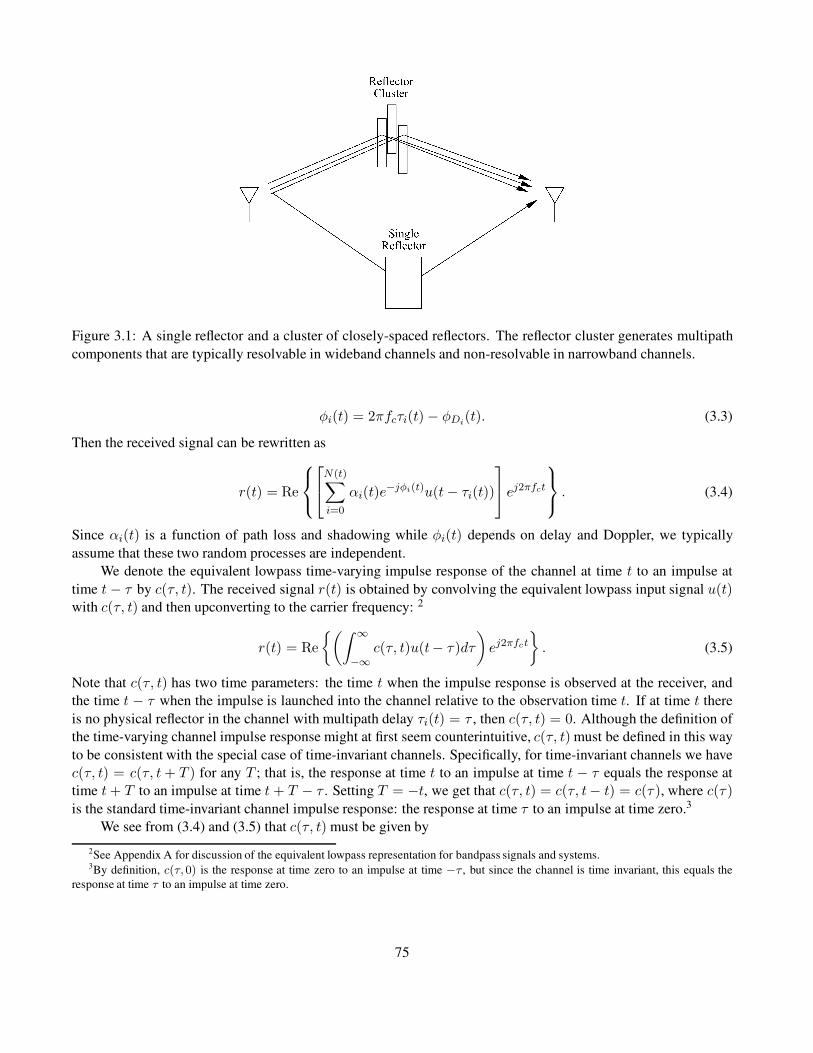
Figure 3.1: A single reflector and a cluster of closely-spaced reflectors. The reflector cluster generates multipath

components that are typically resolvable in wideband channels and non-resolvable in narrowband channels.

φi(t) = 2πfcτi(t) − φDi(t). (3.3)

Then the received signal can be rewritten as

r(t) = Re

N(t)∑

i=0

αi(t)e−jφi(t)u(t− τi(t))

ej2πfct

. (3.4)

Since αi(t) is a function of path loss and shadowing while φi(t) depends on delay and Doppler, we typically

assume that these two random processes are independent.

We denote the equivalent lowpass time-varying impulse response of the channel at time t to an impulse at

time t− τ by c(τ, t). The received signal r(t) is obtained by convolving the equivalent lowpass input signal u(t)with c(τ, t) and then upconverting to the carrier frequency: 2

r(t) = Re

{(∫ ∞

−∞c(τ, t)u(t− τ)dτ

)

ej2πfct

}

. (3.5)

Note that c(τ, t) has two time parameters: the time t when the impulse response is observed at the receiver, and

the time t − τ when the impulse is launched into the channel relative to the observation time t. If at time t there

is no physical reflector in the channel with multipath delay τi(t) = τ , then c(τ, t) = 0. Although the definition of

the time-varying channel impulse response might at first seem counterintuitive, c(τ, t) must be defined in this way

to be consistent with the special case of time-invariant channels. Specifically, for time-invariant channels we have

c(τ, t) = c(τ, t+ T ) for any T ; that is, the response at time t to an impulse at time t − τ equals the response at

time t+ T to an impulse at time t+ T − τ . Setting T = −t, we get that c(τ, t) = c(τ, t− t) = c(τ), where c(τ)

is the standard time-invariant channel impulse response: the response at time τ to an impulse at time zero.3

We see from (3.4) and (3.5) that c(τ, t) must be given by

2See Appendix A for discussion of the equivalent lowpass representation for bandpass signals and systems.3By definition, c(τ,0) is the response at time zero to an impulse at time −τ , but since the channel is time invariant, this equals the

response at time τ to an impulse at time zero.

75

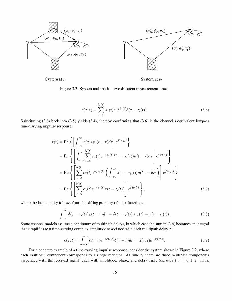
Figure 3.2: System multipath at two different measurement times.

c(τ, t) =

N(t)∑

i=0

αi(t)e−jφi(t)δ(τ − τi(t)). (3.6)

Substituting (3.6) back into (3.5) yields (3.4), thereby confirming that (3.6) is the channel’s equivalent lowpass

time-varying impulse response:

r(t) = Re

{[∫ ∞

−∞c(τ, t)u(t− τ)dτ

]

ej2πfct

}

= Re

∫ ∞

−∞

N(t)∑

i=0

αi(t)e−jφi(t)δ(τ − τi(t))u(t− τ)dτ

ej2πfct

= Re

N(t)∑

i=0

αi(t)e−jφi(t)

(∫ ∞

−∞δ(τ − τi(t))u(t− τ)dτ

)

ej2πfct

= Re

N(t)∑

i=0

αi(t)e−jφi(t)u(t− τi(t))

ej2πfct

, (3.7)

where the last equality follows from the sifting property of delta functions:

∫ ∞

−∞δ(τ − τi(t))u(t− τ)dτ = δ(t− τi(t)) ∗ u(t) = u(t− τi(t)). (3.8)

Some channel models assume a continuum of multipath delays, in which case the sum in (3.6) becomes an integral

that simplifies to a time-varying complex amplitude associated with each multipath delay τ :

c(τ, t) =

∫ ∞

−∞α(ξ, t)e−jφ(ξ,t)δ(τ − ξ)dξ = α(τ, t)e−jφ(τ,t). (3.9)

For a concrete example of a time-varying impulse response, consider the system shown in Figure 3.2, where

each multipath component corresponds to a single reflector. At time t1 there are three multipath components

associated with the received signal, each with amplitude, phase, and delay triple (αi, φi, τi), i = 0, 1, 2. Thus,

76

Figure 3.3: Response of time-varying channel.

impulses that were launched into the channel at time t1 − τi, i = 0, 1, 2, will all be received at time t1, and

impulses launched into the channel at any other time will not be received at t1 (because there is no multipath

component with the corresponding delay). The time-varying impulse response corresponding to t1 equals

c(τ, t1) =

2∑

i=0

αie−jφiδ(τ − τi), (3.10)

and the channel impulse response for t = t1 is shown in Figure 3.3. Figure 3.2 also shows the system at time t2,

where there are two multipath components associated with the received signal having amplitude, phase, and delay

triple (α′i, φ

′i, τ

′i), i = 0, 1. Thus, impulses that were launched into the channel at time t2 − τ ′i , i = 0, 1, will all

be received at time t2, and impulses launched into the channel at any other time will not be received at t2. The

time-varying impulse response at t2 equals

c(τ, t2) =

1∑

i=0

α′ie

−jφ′iδ(τ − τ ′i) (3.11)

and is also shown in Figure 3.3.

If the channel is time invariant, then the time-varying parameters in c(τ, t) become constant and c(τ, t) = c(τ)

is just a function of τ :

c(τ) =N∑

i=0

αie−jφiδ(τ − τi). (3.12)

77

For time-varying channels, the response to an impulse at time t1 is just a shifted version of its response to an

impulse at time t2 6= t1.

Example 3.8: Consider a wireless LAN operating in a factory near a conveyor belt. The transmitter and receiver

have a LOS path between them with gain α0, phase φ0, and delay τ0. Every T0 seconds, a metal item comes

down the conveyor belt, creating an additional reflected signal path with gain α1, phase φ1, and delay τ1. Find the

time-varying impulse response c(τ, t) of this channel.

Solution: For t 6= nT0, n = 1, 2, . . ., the channel impulse response simply corresponds to the LOS path. For

t = nT0, the channel impulse response includes both the LOS and reflected paths. Thus, c(τ, t) is given by

c(τ, t) =

{

α0ejφ0δ(τ − τ0), t 6= nT0,

α0ejφ0δ(τ − τ0) + α1e

jφ1δ(τ − τ1), t = nT0.

Note that, for typical carrier frequencies, the ith multipath component will have fcτi(t) � 1. For example, with

fc = 1 GHz and τi = 50 ns (a typical value for an indoor system), fcτi = 50 � 1. Outdoor wireless systems

have multipath delays much greater than 50 ns, so this property also holds for these systems. If fcτi(t) � 1 then

a small change in the path delay τi(t) can lead to a large phase change in the ith multipath component with phase

φi(t) = 2πfcτi(t) − φDi(t) − φ0. Rapid phase changes in each multipath component give rise to constructive

and destructive addition of the multipath components constituting the received signal, which in turn causes rapid

variation in the received signal strength. This multipath fading phenomenon was exhibited in the deterministic

channel models of Chapter 2 (see, e.g., Figure 2.4 illustrating the received signal power for the two-ray multipath

model). This phenomenon for statistical multipath models will be discussed in more detail in subsequent sections.

The impact of multipath on the received signal depends on whether the spread of time delays associated

with the LOS and different multipath components is large or small relative to the inverse signal bandwidth. If

this channel delay spread is small then the LOS and all multipath components are nonresolvable, leading to the

narrowband fading model described in the next section. If the delay spread is large then some number of the LOS

and multipath components are resolvable, leading to the wideband fading model of Section 3.3. The delay spread

is typically measured relative to the received signal component to which the demodulator is synchronized. Thus,

for the time-invariant channel model of (3.12), if the demodulator synchronizes to the LOS signal component,

which has the smallest delay τ0, then the delay spread is a constant given by Tm = maxi[τi − τ0]. However,

if the demodulator synchronizes to a multipath component with delay equal to the mean delay τ , then the delay

spread is given by Tm = maxi |τi − τ |. In time-varying channels the multipath delays vary with time, so the

delay spread Tm becomes a random variable. Moreover, some received multipath components have significantly

lower power than others, so it’s not clear how the delay associated with such components should be used in the

characterization of delay spread. In particular, if the power of a multipath component is below the noise floor then

it should not significantly contribute to the delay spread. These issues are typically dealt with by characterizing

the delay spread relative to the channel power delay profile, defined in Section 3.3.2. Specifically, two common

characterizations of channel delay spread – average delay spread and rms (root mean square) delay spread – are

determined from the power delay profile. Other characterizations of delay spread, such as excees delay spread,

the delay window, and the delay interval, are sometimes used as well [1, Chap. 5.4.1; 2, Chap. 6.7.1]. The exact

characterization of delay spread is not that important for understanding the general impact of delay spread on

multipath channels, as long as the characterization roughly measures the delay associated with significant multipath

components. We will adopt the rms delay spread for our characterization as it is the one most widely used in the

literature. Assuming the demodulator synchronizes to a signal component at the average delay spread, the rms

78

delay spread is a good measure of the variation about this average. Channel delay spread is highly dependent on

the propagation environment. In indoor channels delay spread typically ranges from 10 to 1000 nanoseconds, in

urban microcells it ranges from 1–10 microseconds, and in rural macrocells is ranges from 10–100 microseconds

[1, Chap. 5].

3.2 Narrowband Fading Model

Suppose the delay spread Tm of a channel is small relative to the inverse baseband signal bandwidth Bu of the

transmitted signal; that is, suppose Tm � B−1u . We refer to the fading in this scenario as narrowband fading

which is a function of both the signal bandwidth Bu and the channel delay spread Tm. As discussed previously,

the delay spread Tm for time-varying channels is usually characterized by the rms delay spread, but it can also

be characterized in other ways. Under most delay spread characterizations, Tm � B−1u implies that the delay

associated with the ith multipath component τi ≤ Tm for all i, so u(t − τi) ≈ u(t) for all i. Since in the

narrowband fading model the delay associated with all multipath components results in minimal signal distortion

in time, we say the channel under this model is nondispersive. We can rewrite (3.4) as

r(t) = Re

{

u(t)ej2πfct

(

∑

i

αi(t)e−jφi(t)

)}

. (3.13)

Equation (3.13) differs from the original transmitted signal by the complex scale factor in large parentheses. This

scale factor is independent of the transmitted signal s(t) and, in particular, of the equivalent lowpass signal u(t)as long as the narrowband assumption Tm � 1/Bu is satisfied. In order to characterize the random scale factor

caused by the multipath, we choose s(t) to be an unmodulated carrier with random phase offset φ0:

s(t) = Re{ej(2πfct+φ0)} = cos(2πfct+ φ0), (3.14)

which is narrowband for any Tm.

With this assumption the received signal becomes

r(t) = Re

N(t)∑

i=0

αi(t)e−jφi(t)

ej2πfct

= rI(t) cos(2πfct) − rQ(t) sin(2πfct), (3.15)

where the in-phase and quadrature components are given by

rI(t) =

N(t)∑

i=0

αi(t) cosφi(t), (3.16)

rQ(t) =

N(t)∑

i=0

αi(t) sinφi(t) (3.17)

and where the phase term

φi(t) = 2πfcτi(t) − φDi(t) − φ0 (3.18)

now incorporates the phase offset φ0 as well as the effects of delay and Doppler.

Suppose N (t) is large and all multipath signal components as well as the LOS component (if it is nonzero)

have random amplitudes with approximately the same distribution, and similarly for the random phases of each

79

component. Then, given that αi(t) and φi(t) are also independent for different components, we can invoke the

Central Limit Theorem (CLT) for sums of independent identically-distributed (i.i.d.) random variables to approx-

imate rI(t) and rQ(t) as jointly Gaussian random processes. The Gaussian property also holds for small N (t) if

the αi(t) are Rayleigh distributed (given in (3.33) below) and the φi(t) are uniformly distributed on [−π, π]. This

happens, again by the CLT, when the ith multipath component results from a reflection cluster with a large number

of nonresolvable multipath components [3]. If the LoS or any of the multipath components has a much larger

amplitude than the average multipath component amplitude, then this component dominates the received signal;

hence the Gaussian approximation is no longer applicable as the terms in (3.15) are not i.i.d.

3.2.1 Autocorrelation, Cross-Correlation, and Power Spectral Density

We now derive the autocorrelation and cross-correlation of the in-phase and quadrature received signal components

rI(t) and rQ(t), as well as the received signal r(t). We focus on these correlations over a time period where the

transmitter or receiver moves on the order of a few signal wavelengths. As we will see, multipath can cause

the received signal to completely decorrelate over a signal wavelength due to changes in phase of the individual

multipath components such that they combine either constructively or destructively. Our derivations of these

correlations are based on some key assumptions that generally apply to propagation models without a dominant

LOS component such that all nonzero terms in (3.15) are approximately i.i.d. We will also determine the power

spectral density (PSD) of the received signal under certain assumptions that make its autocorrelation function

time-invariant. In this case the PSD is just the Fourier transform of the autocorrelation function.

We will assume throughout this section that the amplitudeαi(t), multipath delay τi(t) = xi(t)/c, and Doppler

frequency fDi(t) = v(t) cosθi(t)/λ are changing slowly enough to be considered constant over the time interval τ

for which we compute the autocorrelation and cross-correlation. This is generally true for τ ≈ λ/v corresponding

to the time over which the transmitter or receiver travels a distance roughly equal to the signal wavelength λ for

travel velocity v. In particular, over such a short distance the number of multipath components N (t) = N doesn’t

change. Then for each of these multipath components, since the shadowing associated with αi(t) decorrelates over

distance Xc which is generally much bigger than λ, αi(t) ≈ αi for some constant αi. Similarly, the distance a

given multipath component travels, the component’s AoA, and the velocity of the transmitter or receiver change

little over the time interval τ , and hence we can assume τi(t) ≈ τi for some average delay τi and fDi(t) ≈ fDi

for

some average Doppler frequency fDi. With a constant Doppler frequency, the Doppler phase shift4 is φDi

(t) =∫ t0 2πfDi

dν = 2πfDit and the phase of the ith multipath component becomes φi(t) = 2πfcτi − 2πfDi

t− φ0.

We now make a key assumption: we assume that, for the ith multipath component, the term 2πfcτi in φi(t)

changes rapidly relative to all other phase terms in the expression. This is a reasonable assumption because fc is

large and hence the term 2πfcτi can go through a 360◦ rotation for a small change in multipath delay τi. Under

this assumption, φi(t) is uniformly distributed on [−π, π]. Thus

E[rI(t)] = E

[

∑

i

αi cosφi(t)

]

=∑

i

E[αi]E[cosφi(t)] = 0, (3.19)

where the second equality follows from the independence of αi and φi(t) and the last equality follows from the

uniform distribution on φi(t). Similarly we can show that E[rQ(t)] = 0. Thus, the received signal also has

E[r(t)] = 0: it is a zero-mean Gaussian process. If there is a dominant LOS component in the channel then the

phase of the received signal is dominated by the phase of the LOS component, which can be determined at the

receiver, so the assumption of a random uniform phase no longer holds.

Consider now the autocorrelation ArI (t, t + τ) = E[rI(t)rI(t + τ)] of the in-phase component. Using the

independence of αi and φi(t), the independence of φi(t) and φj(t) (i 6= j), and the uniform distribution of φi(t),

4We shall assume a Doppler phase shift at t = 0 of zero for simplicity, because this phase offset will not affect the analysis.

80

we get that

ArI (t, t+ τ) = E

∑

i

αi cosφi(t)∑

j

αj cosφj(t+ τ)

=∑

i

∑

j

E[αiαj]E[cosφi(t) cosφj(t+ τ)]

=∑

i

E[α2i ]E[cosφi(t) cosφi(t+ τ)]. (3.20)

Since φi(t) = 2πfcτi − 2πfDit− φ0 and φi(t+ τ) = 2πfcτi − 2πfDi

(t+ τ) − φ0 we have

E[cosφi(t) cosφi(t+ τ)] = .5E[cos 2πfDiτ ] + .5E[cos(4πfcτi − 4πfDi

t− 2πfDiτ − 2φ0)]. (3.21)

Because 2πfcτi changes rapidly relative to all other phase terms and is uniformly distributed modulo 2π, the

second expectation term in (3.21) is zero and thus

ArI (t, t+ τ) = .5∑

i

E[α2i ]E[cos(2πfDi

τ)] = .5∑

i

E[α2i ] cos

(

2πvτ

λcos θi

)

, (3.22)

since fDi= v cos(θi)/λ is assumed fixed. Observe that ArI (t, t + τ) depends only on τ and hence rI(t) is a

wide-sense stationary (WSS) random process. Thus we can write ArI (t, t+ τ) = ArI (τ) as a function of τ only.

Moreover, using a similar derivation as (3.22) we can show that the quadrature component is also WSS with the

same autocorrelation as ArI (τ), so ArI (τ) = ArQ(τ).

We now consider the cross-correlation between the in-phase and quadrature components. Using the same

trigonometric properties as in the derivation of (3.22) and the fact that 2πfcτi is uniformly distributed we get

ArI ,rQ(t, t+ τ) = E[rI(t)rQ(t+ τ)] = −.5∑

i

E[α2i ] sin

(

2πvτ

λcos θi

)

(3.23)

and

ArQ,rI (t, t+ τ) = E[rQ(t)rI(t+ τ)] = .5∑

i

E[α2i ] sin

(

2πvτ

λcos θi

)

. (3.24)

We see from (3.23) and (3.24) that these cross-corrections only depend on τ so we can write these as ArI ,rQ(t, t+τ) = ArI ,rQ(τ) and ArQ,rI (t, t + τ) = ArQ,rI (τ). Moreover, we see from these equations that ArI ,rQ(τ) =−ArQ ,rI (τ). Finally, setting τ = 0 we see that ArI ,rQ(0) = −ArQ ,rI (0) = 0. Thus, rI(t) and rQ(t) are

uncorrelated and, since they are jointly Gaussian processes, this means they are independent.

We now consider the autocorrelation of the received signal

r(t) = rI(t) cos(2πfct) − rQ(t) sin(2πfct).

81

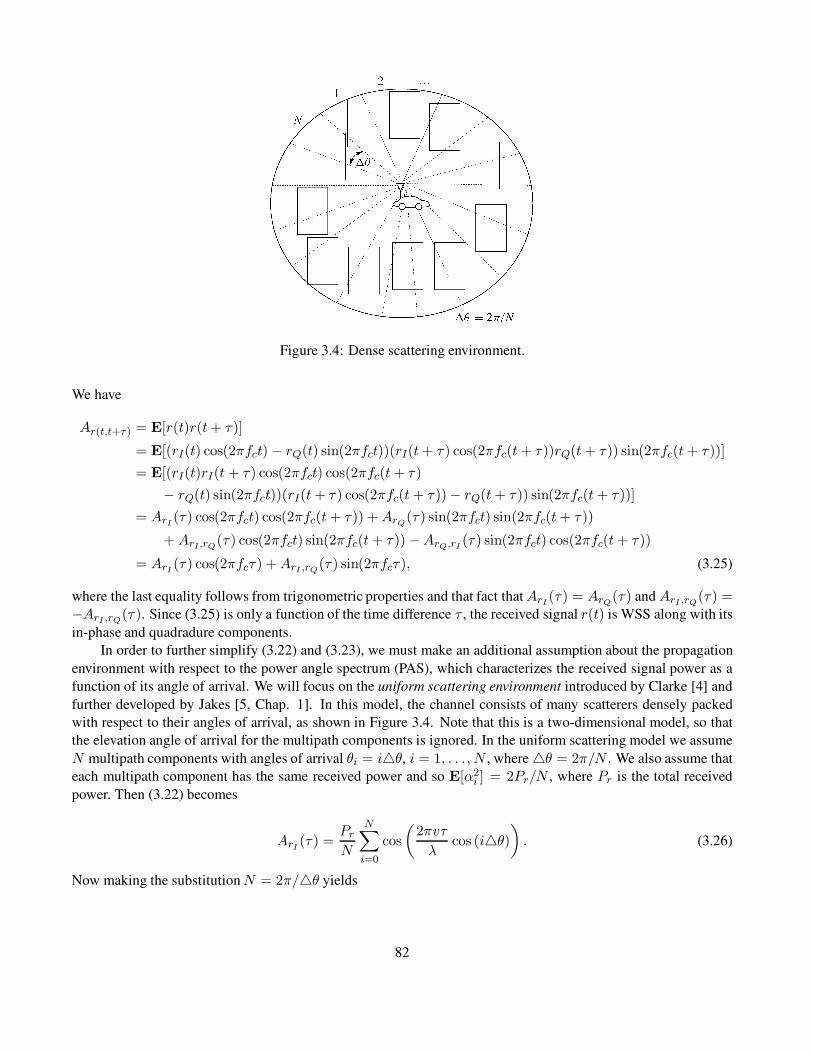
Figure 3.4: Dense scattering environment.

We have

Ar(t,t+τ ) = E[r(t)r(t+ τ)]

= E[(rI(t) cos(2πfct) − rQ(t) sin(2πfct))(rI(t+ τ) cos(2πfc(t+ τ))rQ(t+ τ)) sin(2πfc(t+ τ))]

= E[(rI(t)rI(t+ τ) cos(2πfct) cos(2πfc(t+ τ)

− rQ(t) sin(2πfct))(rI(t+ τ) cos(2πfc(t+ τ))− rQ(t+ τ)) sin(2πfc(t+ τ))]

= ArI (τ) cos(2πfct) cos(2πfc(t+ τ)) + ArQ(τ) sin(2πfct) sin(2πfc(t+ τ))

+ ArI ,rQ(τ) cos(2πfct) sin(2πfc(t+ τ)) −ArQ,rI (τ) sin(2πfct) cos(2πfc(t+ τ))

= ArI (τ) cos(2πfcτ) +ArI ,rQ(τ) sin(2πfcτ), (3.25)

where the last equality follows from trigonometric properties and that fact thatArI (τ) = ArQ(τ) and ArI ,rQ(τ) =−ArI ,rQ(τ). Since (3.25) is only a function of the time difference τ , the received signal r(t) is WSS along with its

in-phase and quadradure components.

In order to further simplify (3.22) and (3.23), we must make an additional assumption about the propagation

environment with respect to the power angle spectrum (PAS), which characterizes the received signal power as a

function of its angle of arrival. We will focus on the uniform scattering environment introduced by Clarke [4] and

further developed by Jakes [5, Chap. 1]. In this model, the channel consists of many scatterers densely packed

with respect to their angles of arrival, as shown in Figure 3.4. Note that this is a two-dimensional model, so that

the elevation angle of arrival for the multipath components is ignored. In the uniform scattering model we assume

N multipath components with angles of arrival θi = i4θ, i = 1, . . . , N , where 4θ = 2π/N . We also assume that

each multipath component has the same received power and so E[α2i ] = 2Pr/N , where Pr is the total received

power. Then (3.22) becomes

ArI (τ) =PrN

N∑

i=0

cos

(

2πvτ

λcos (i4θ)

)

. (3.26)

Now making the substitutionN = 2π/4θ yields

82

ArI (τ) =Pr2π

N∑

i=0

cos

(

2πvτ

λcos (i4θ)

)

4θ. (3.27)

We now take the limit as the number of scatterers grows to infinity, which corresponds to uniform scattering from

all directions. Then N → ∞,4θ → 0, and the summation in (3.27) becomes an integral:

ArI (τ) =Pr2π

∫ 2π

0cos

(

2πvτ

λcos θ

)

dθ = PrJ0(2πfDτ), (3.28)

where fD = 2πv/λ and

J0(x) =1

π

∫ π

0e−jx cos θdθ

Figure 3.5: Bessel function versus fDτ .

is the Bessel function of zeroth order.5 Similarly, for this uniform scattering environment,

ArI ,rQ(τ) =Pr2π

∫

sin

(

2πvτ

λcos(θ)

)

dθ = 0. (3.29)

A plot of J0(2πfDτ) is shown in Figure 3.5. There are several interesting observations to make from this plot.

First we see that the autocorrelation is zero for fDτ ≈ .4 or, equivalently, for vτ ≈ .4λ. Thus, the signal decorre-

lates over a distance of approximately one half wavelength under the uniform θi assumption. This approximation

is commonly used as a rule of thumb to determine many system parameters of interest. For example, we will see

in Chapter 7 that independent fading paths obtained from multiple antennas can be combined to remove some of

the negative effects of fading. For independent fading the antenna spacing must be .4λ based on the analysis here.

5Equation (3.28) can also be derived by assuming that 2πvτ cos θi/λ in (3.22) and (3.23) is random with θi uniformly distributed, and

then taking expectations with respect to θi . However, based on the underlying physical model, θi can be uniformly distributed only in a

dense scattering environment. So the derivations are equivalent.

83

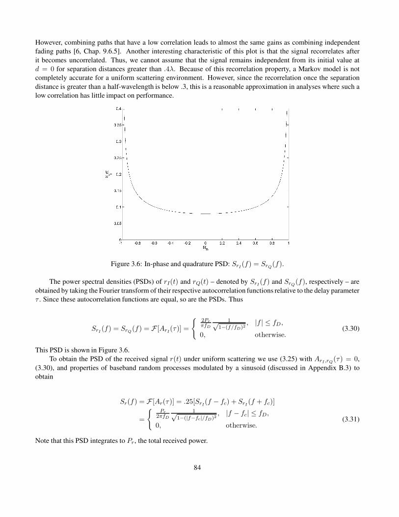
However, combining paths that have a low correlation leads to almost the same gains as combining independent

fading paths [6, Chap. 9.6.5]. Another interesting characteristic of this plot is that the signal recorrelates after

it becomes uncorrelated. Thus, we cannot assume that the signal remains independent from its initial value at

d = 0 for separation distances greater than .4λ. Because of this recorrelation property, a Markov model is not

completely accurate for a uniform scattering environment. However, since the recorrelation once the separation

distance is greater than a half-wavelength is below .3, this is a reasonable approximation in analyses where such a

low correlation has little impact on performance.

Figure 3.6: In-phase and quadrature PSD: SrI (f) = SrQ(f).

The power spectral densities (PSDs) of rI(t) and rQ(t) – denoted by SrI (f) and SrQ(f), respectively – are

obtained by taking the Fourier transform of their respective autocorrelation functions relative to the delay parameter

τ . Since these autocorrelation functions are equal, so are the PSDs. Thus

SrI (f) = SrQ(f) = F [ArI(τ)] =

{

2Pr

πfD

1√1−(f/fD)2

, |f | ≤ fD ,

0, otherwise.(3.30)

This PSD is shown in Figure 3.6.

To obtain the PSD of the received signal r(t) under uniform scattering we use (3.25) with ArI ,rQ(τ) = 0,

(3.30), and properties of baseband random processes modulated by a sinusoid (discussed in Appendix B.3) to

obtain

Sr(f) = F [Ar(τ)] = .25[SrI(f − fc) + SrI (f + fc)]

=

{

Pr

2πfD

1√1−(|f−fc|/fD)2

, |f − fc| ≤ fD,

0, otherwise.(3.31)

Note that this PSD integrates to Pr, the total received power.

84

Since the PSD models the power density associated with multipath components as a function of their Doppler

frequency, it can be viewed as the probability density function (pdf) of the random frequency due to Doppler asso-

ciated with multipath. We see from Figure 3.6 that the PSD SrI (f) goes to infinity at f = ±fD and, consequently,

the PSD Sr(f) goes to infinity at f = ±fc ± fD. This will not be true in practice, since the uniform scattering

model is just an approximation, but for environments with dense scatterers the PSD will generally be maximized at

frequencies close to the maximum Doppler frequency. The intuition for this behavior comes from the nature of the

cosine function and the fact that (under our assumptions) the PSD corresponds to the pdf of the random Doppler

frequency fD(θ).

Figure 3.7: Cosine and PSD approximation by straight line segments.

To see this, note that the uniform scattering assumption is based on many scattered paths arriving uniformly

from all angles with the same average power. Thus, θ for a randomly selected path can be regarded as a uniform

random variable on [0, 2π]. The pdf pfD(θ)(f) of the random Doppler frequency fD(θ) can then be obtained

from the pdf of θ. By definition, pfD(θ)(f) is proportional to the density of scatterers at Doppler frequency f .

Hence, SrI (f) is also proportional to this density, and we can characterize the PSD from the pdf pfD(θ)(f). For

this characterization, in Figure 3.7 we plot fD(θ) = fD cos(θ) = vλ cos(θ) along with a (dashed) straight-line

segment approximation fD

(θ) to fD(θ). On the right in this figure we plot the PSD SrI (f) along with a dashed

straight-line segment approximation to it, SrI (f), which corresponds to the Doppler approximation fD

(θ). We

see that cos(θ) ≈ ±1 for a relatively large range of θ-values. Thus, multipath components with angles of arrival

in this range of values have Doppler frequency fD(θ) ≈ ±fD, so the power associated with all of these multipath

components will add together in the PSD at f ≈ fD. This is shown in our approximation by the fact that the

segments where fD

(θ) = ±fD on the left lead to delta functions at ±fD in the PSD approximation SrI (f) on the

right. The segments where fD

(θ) has uniform slope on the left lead to the flat part of SrI (f) on the right, since

there is one multipath component contributing power at each angular increment. This explains the shape of SrI (f)

under uniform scattering. Formulas for the autocorrelation and PSD in nonuniform scattering – corresponding to

more typical microcell and indoor environments – can be found in [5, Chap. 1; 7, Chap. 2]. Three-dimensional

channel models that incorporate elevation angle are described in [8] and the references therein.

The PSD is useful in constructing simulations for the fading process. A common method for simulating the

envelope of a narrowband fading process is to pass two independent white Gaussian noise sources with PSD N0/2

through lowpass filters with a frequency response H(f) that satisfies

SrI (f) = SrQ(f) =N0

2|H(f)|2. (3.32)

85

The filter outputs then correspond, respectively, to the in-phase and quadrature components of the narrowband

fading process with PSDs SrI (f) and SrQ(f). A similar procedure using discrete filters can be used to generate

discrete fading processes. Most communication simulation packages (e.g. the Matlab communications toolbox)

have standard modules that simulate narrowband fading based on this method. More details on this simulation

method, as well as alternative methods, can be found in [1, 7, 9, 10].

We have now completed our model for the three characteristics of power versus distance exhibited in nar-

rowband wireless channels. These characteristics are illustrated in Figure 3.8, adding narrowband fading to the

single-slope path loss and log-normal shadowing models developed in Chapter 2. In this figure we see the signal

power due to path loss decreasing at a slope of −10γ relative to log1 0d/d0 for γ the path-loss exponent and d0

the reference distance at which the path loss equals the constant K. The more rapid variations due to shadowing

change on the order of the decorrelation distanceXc, and the very rapid variations due to multipath fading change

on the order of half the signal wavelength. If we blow up a small segment of this figure over distances where path

loss and shadowing are constant we obtain Figure 3.9, which plots the dB value of Pr/Pt versus linear distance

d = vt (not log distance). In this figure the average value of Pr/Pt is normalized to 0 dB. A mobile receiver trav-

eling at fixed velocity v would experience stationary and ergodic received power variations over time as illustrated

in this figure.

Figure 3.8: Combined single-slope path loss, log-normal shadowing, and narrowband fading.

3.2.2 Envelope and Power Distributions

We now consider the distributionof the envelope and power for the narrowband received signal r(t) = rI(t) cos(2πfct)−rQ(t) sin(2πfct). It can be shown that, for any two Gaussian random variables X and Y , both with mean zero

and equal variance σ2, Z =√X2 + Y 2 is Rayleigh distributed and Z2 is exponentially distributed. We have

seen that, for φi(t) uniformly distributed, rI and rQ are both zero-mean Gaussian random variables. If we as-

sume a variance of σ2 = .5∑

iE[α2i ] for both in-phase and quadrature components, then the signal envelope

z(t) = |r(t)| =√

r2I (t) + r2Q(t) is Rayleigh distributed with distribution

pZ(z) =2z

Pzexp

[

− z2

Pz

]

=z

σ2exp

[

− z2

2σ2

]

, z ≥ 0, (3.33)

where Pz = 2σ2 is the power of z(t).

We obtain the power distribution by making the change of variables z2(t) = |r(t)|2 in (3.33) to obtain

86

Figure 3.9: Narrowband fading.

pZ2(x) =1

Pze−x/Pz =

1

2σ2e−x/2σ

2, x ≥ 0. (3.34)

i.e. the power in z(t) is exponentially distributed with mean Pz = 2σ2. Since z(t) is the envelope of r(t), it has

twice the power of r(t). Thus, r(t) has a Rayleigh-distributed amplitude and uniformly-distributed power with

mean Pr = .5Pz = σ2. The equivalent lowpass signal for r(t) is given by rLP (t) = rI(t) + jrQ(t), which has

the same power as z(t) and phase θ = arctan (rQ(t)/rI(t)). For rI(t) and rQ(t) uncorrelated Gaussian random

variables we can show that θ is uniformly distributed and independent of |rLP |.

Example 3.9: Consider a channel with Rayleigh fading and average received power Pr = 20 dBm. Find the

probability that the received power is below 10 dBm.

Solution: We have Pr = 20 dBm = 100 mW. We want to find the probability that Z2 < 10 dBm = 10 mW.

Thus

p(Z2 < 10) =

∫ 10

0

1

100e−x/100dx = .095.

If the channel has a LOS component with a much larger signal power than the other multipath components, then

rI(t) and rQ(t) are not zero-mean random processes. That is because the average signal power is dominated by

the LOS component, with small fluctuations about this average due to constructive and destructive addition of

the multipath components. In this scenario the received signal equals the superposition of a complex Gaussian

component and a higher-power LOS component. The signal envelope in this case can be shown to have a Rician

distribution [11] given by

pZ(z) =z

σ2exp

[−(z2 + s2)

2σ2

]

I0

(zs

σ2

)

, z ≥ 0, (3.35)

where 2σ2 =∑

i,i6=0 E[α2i ] is the average power in the non-LOS multipath components and s2 = α2

0 is the power

in the LOS component. The function I0 is the modified Bessel function of zeroth order. The average received

power in the Rician fading is given by

87

Pr =

∫ ∞

0z2pZ(z)dz = s2 + 2σ2. (3.36)

The Rician distribution is often described in terms of a fading parameter K, defined by

K =s2

2σ2. (3.37)

Thus,K is the ratio of the power in the LOS component to the power in the other (non-LOS) multipath components,

which is typically a random variable. For K = 0 we have Rayleigh fading and for K = ∞ we have no fading

(i.e., a channel with no multipath and only a LOS component). The fading parameter K is therefore a measure of

the severity of the fading: a small K implies severe fading, a large K implies relatively mild fading. Making the

substitutions s2 = KPr/(K + 1) and 2σ2 = Pr/(K + 1), we can write the Rician distribution in terms of K and

Pr as

pZ(z) =2z(K + 1)

Prexp

[

−K − (K + 1)z2

Pr

]

I0

2Z

√

K(K + 1)

Pr

, z ≥ 0. (3.38)

Both the Rayleigh and Rician distributions can be obtained by using mathematics to capture the underlying

physical properties of the channel models [3, 11]. However, some experimental data does not fit well into either of

these distributions. Thus, a more general fading distribution was developed whose parameters can be adjusted to

fit a variety of empirical measurements. This distribution is called the Nakagami fading distribution and is given

by

pZ(z) =2mmz2m−1

Γ(m)Pmrexp

[−mz2

Pr

]

, m ≥ .5, (3.39)

where Pr is the average received power and Γ(·) is the Gamma function. The Nakagami distribution is param-

eterized by Pr and the fading parameter m. For m = 1 the distribution in (3.39) reduces to Rayleigh fading.

For m = (K + 1)2/(2K + 1) the distribution in (3.39) is approximately Rician fading with parameter K. For

m = ∞ there is no fading: Z =√Pr is a constant. Thus, the Nakagami distribution can model both Rayleigh

and Rician distributions as well as more general ones. Note that some empirical measurements support values of

the m-parameter less than unity, in which case the Nakagami fading causes more severe performance degradation

than Rayleigh fading. The power distribution for Nakagami fading, obtained by a change of variables, is given by

pZ2(x) =

(

m

Pr

)m xm−1

Γ(m)exp

[−mxPr

]

. (3.40)

While narrowband fading is often modeled using the Rayleigh, Rician, or Nakagami distribution, these distri-

butions are not accurate for many environments that arise in practice. This has led to several important extensions

of these models [6]. In particular, the Hoyt (or Nakagami-q) distribution models narrowband fading of the received

signal envelope assuming instaneous values of the in-phase and quadrature components are zero-mean Gaussian

random variables with unequal variances. The Beckman distribution generalizes the Hoyt model such that the in-

stantaneous in-phase and quadrature components are Gaussian random variables with unequal means and unequal

variances. The Weibull fading model generalizes both Rayleigh and exponential distributions, and with proper

parameterization has been shown to fit with with experimental data. The pdf formulas for the Hoyt, Beckman, and

Weibull distributions can be found in [6].

88

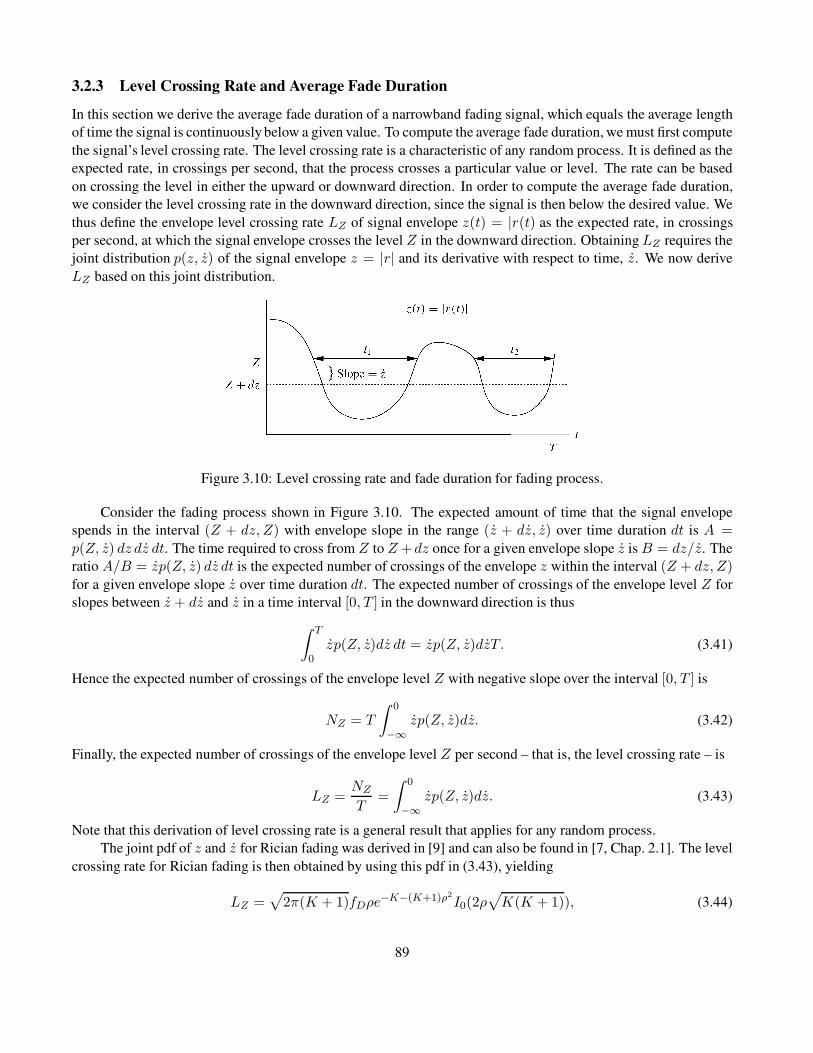
3.2.3 Level Crossing Rate and Average Fade Duration

In this section we derive the average fade duration of a narrowband fading signal, which equals the average length

of time the signal is continuously below a given value. To compute the average fade duration, we must first compute

the signal’s level crossing rate. The level crossing rate is a characteristic of any random process. It is defined as the

expected rate, in crossings per second, that the process crosses a particular value or level. The rate can be based

on crossing the level in either the upward or downward direction. In order to compute the average fade duration,

we consider the level crossing rate in the downward direction, since the signal is then below the desired value. We

thus define the envelope level crossing rate LZ of signal envelope z(t) = |r(t) as the expected rate, in crossings

per second, at which the signal envelope crosses the level Z in the downward direction. ObtainingLZ requires the

joint distribution p(z, z) of the signal envelope z = |r| and its derivative with respect to time, z. We now derive

LZ based on this joint distribution.

Figure 3.10: Level crossing rate and fade duration for fading process.

Consider the fading process shown in Figure 3.10. The expected amount of time that the signal envelope

spends in the interval (Z + dz, Z) with envelope slope in the range (z + dz, z) over time duration dt is A =

p(Z, z) dz dz dt. The time required to cross from Z to Z +dz once for a given envelope slope z is B = dz/z. The

ratio A/B = zp(Z, z) dz dt is the expected number of crossings of the envelope z within the interval (Z + dz, Z)

for a given envelope slope z over time duration dt. The expected number of crossings of the envelope level Z for

slopes between z + dz and z in a time interval [0, T ] in the downward direction is thus

∫ T

0zp(Z, z)dz dt = zp(Z, z)dzT. (3.41)

Hence the expected number of crossings of the envelope level Z with negative slope over the interval [0, T ] is

NZ = T

∫ 0

−∞zp(Z, z)dz. (3.42)

Finally, the expected number of crossings of the envelope level Z per second – that is, the level crossing rate – is

LZ =NZ

T=

∫ 0

−∞zp(Z, z)dz. (3.43)

Note that this derivation of level crossing rate is a general result that applies for any random process.

The joint pdf of z and z for Rician fading was derived in [9] and can also be found in [7, Chap. 2.1]. The level

crossing rate for Rician fading is then obtained by using this pdf in (3.43), yielding

LZ =√

2π(K + 1)fDρe−K−(K+1)ρ2I0(2ρ

√

K(K + 1)), (3.44)

89

where ρ = Z/√

Pr . For Rayleigh fading (K = 0) the level crossing rate simplifies to

LZ =√

2πfDρe−ρ2 . (3.45)

We define the average signal fade duration as the average time that the signal envelope stays below a given

target level Z. This target level is often obtained from the signal amplitude or power level required for a given

performance metric such as bit error rate. If the signal amplitude or power falls below its target then we say the

system is in outage. Let ti denote the duration of the ith fade below level Z over a time interval [0, T ], as illustrated

in Figure 3.10. Thus ti equals the length of time that the signal envelope stays below Z on its ith crossing. Since

z(t) is stationary and ergodic, for T sufficiently large we have

p(z(t) < Z) =1

T

∑

i

ti. (3.46)

Thus, for T sufficiently large, the average fade duration is

tZ =1

TLZ

LZT∑

i=1

ti ≈p(z(t) < Z)

LZ. (3.47)

Using the Rayleigh distribution for p(z(t) < Z) then yields

tZ =eρ

2 − 1

ρfD√

2π(3.48)

with ρ = Z/√

Pr. Note that (3.48) is the average fade duration for the signal envelope (amplitude) level with Z

the target amplitude and√

Pr the average envelope level. By a change of variables it is easily shown that (3.48)

also yields the average fade duration for the signal power level with ρ =√

P0/Pr, where P0 is the target power

level and Pr is the average power level. The average fade duration (3.48) decreases with the Doppler frequency

fD, since as a channel changes more quickly it remains below a given fade level for a shorter period of time. The

average fade duration also generally increases with ρ for ρ � 1. That is because the signal is more likely to be

below the target as the target level increases relative to the average. The average fade duration for Rician fading is

more difficult to compute; it can be found in [7, Chap. 1.4].

The average fade duration indicates the number of bits or symbols affected by a deep fade. Specifically,

consider an uncoded system with bit time Tb. Suppose the probability of bit error is high when z < Z. In this case,

if Tb ≈ tZ then the system will likely experience single error events, where bits that are received in error have the

previous and subsequent bits received correctly (since z > Z for these bits). On the other hand, if Tb � tZ then

many subsequent bits are received with z < Z, so large bursts of errors are likely. Finally, if Tb � tZ then, since

the fading is integrated over a bit time in the demodulator, the fading gets averaged out and so can be neglected.

These issues will be explored in more detail in Chapter 8, where we consider coding and interleaving.

Example 3.10: Consider a voice system with acceptable BER when the received signal power is at or above half

its average value. If the BER is below its acceptable level for more than 120 ms, users will turn off their phone.

Find the range of Doppler values in a Rayleigh fading channel such that the average time duration when users have

unacceptable voice quality is less than t = 60 ms.

Solution: The target received signal value is half the average, so P0 = .5Pr and thus ρ =√

5. We require

tZ =e.5 − 1

fD√π

≤ t = .060

90

and thus fD ≥ (e.5 − 1)/(.060√π) = 6.1 Hz.

3.2.4 Block-Fading and Finite-State Markov Fading

The complex mathematical characterization of the narrowband fading model described in the previous sections

can be difficult to incorporate into wireless performance analysis. Therefore, simpler models that capture the main

features of narrowband fading channels are often used for these analytical calculations. This section describes two

such models: block-fading and finite-state Markov fading channels.

In a block-fading channel, the channel SNR γ is assumed constant over some period of time T called the

block time. In this model we denote γ(i) as the channel SNR over the ith block. It is typically assumed that γ(i) is

i.i.d. between blocks although a more complex model capturing correlation of the channel gain across blocks can

also be used. Often T is set equal to an integer number of modulation symbol times Ts: T = NTs where NTsis approximately equal to the channel coherence time defined in Section 3.3.4 below. A rapidly-fading channel

might be approximated by setting N = 1 such that the fading is constant over each symbol time and changes to

a different i.i.d. value between subsequent symbols. A variation on the block-fading model allows for continuous

variation of the channel gain within a block, typically using the model of Section 3.2.1, with an abrupt transition

to an independent channel gain at each block time. This model is often used for systems where blocks of symbols

are sent intermittently and hence each block experiences a completely different propagation environment.

The finite-state Markov channel (FSMC) is a special case of block-fading where a finite set of channel SNR

values is assumed with a Markov transition probability of the fading between blocks. Specifically in the FSMC

the channel SNR is assumed to belong to a finite set of values, called channel states, and to follow a discrete-

time Markov process with time discretized to the block time T . The channel varies over its possible states at

each interval T according to a set of Markov transition probabilities. FSMCs have been used to approximate both

mathematical and experimental fading models, including satellite channels [12], indoor channels [13], Rayleigh

fading channels [14, 15], Rician fading channels [16], and Nakagami-m fading channels [17]. They have also been

used for system design and system performance analysis [15, 18]. First-order FSMC models are deficient when the

fading recorrelation affects performance analysis, in which case higher-order models are used. The FSMC models

for fading typically model amplitude variations only, although there has been some work on FSMC models for

phase in fading [19] or phase-noisy channels [20].

A detailed FSMC model for Rayleigh fading was developed in [14]. In this model the time-varying SNR γ

associated with the Rayleigh fading lies in the range 0 ≤ γ < infty. The FSMC model discretizes this fading

range into regions so that the jth region Rj is defined as Rj = {γ : Aj ≤ γ < Aj+1}, where the region

boundaries {Aj} and the total number of fade regions are parameters of the model. This model assumes that γstays within the same region over time interval T and can only transition to the same region or adjacent regions

at time T + 1. Thus, given that the channel is in state Rj at time T , at the next time interval the channel can

only transition to Rj−1, Rj, or Rj+1 – a reasonable assumption when fDT is small. Under this assumption, the

transition probabilities between regions are derived in [14] as

pj,j+1 =Lj+1T

πj, pj,j−1 =

LjT

πj, pj,j = 1 − pj,j+1 − pj,j−1, (3.49)

where Lj is the level crossing rate at Aj and πj is the steady-state distribution corresponding to the jth region:

πj = p(γ ∈ Rj) = p(Aj ≤ γ < Aj+1).

91

3.3 Wideband Fading Model

Suppose the transmitted signal is not narrowband relative to the inverse delay spread. Since the signal bandwidth

B ≈ 1/T for T the signal duration, the received signal will have duration T + Tm >> T for Tm is the delay

spread. Thus, the duration of the received signal will be significantly increased, and we refer to the channel in

this case as a dispersive channel. This phenomenon is illustrated in Figure 3.11. In the figure, a pulse of width

T is transmitted over a multipath channel. As discussed in Chapter 5, linear modulation consists of a train of

pulses where each pulse carries information in its amplitude and/or phase corresponding to a data bit or symbol.6

If the multipath delay spread Tm � T then the multipath components are received roughly on top of one another,

as shown in the upper right of the figure. Hence the channel is nondispersive. The resulting constructive and

destructive interference causes narrowband fading of the pulse, but there is little time spreading of the pulse and

therefore little interference with a subsequently transmitted pulse. On the other hand, if the multipath delay spread

Tm � T , then each of the different multipath components can be resolved, as shown in the lower right of the

figure. However, these multipath components interfere with subsequently transmitted pulses (dashed pulses in the

figure). This effect is called intersymbol interference (ISI).

Figure 3.11: Multipath resolution.

There are several techniques to mitigate the distortion due to multipath delay spread, including equalization,

multicarrier modulation, and spread spectrum, which are discussed in Chapters 11–13. Mitigating ISI is not nec-

essary if T � Tm. However, most wireless systems require data rates R ≈ 1/T to be much greater than 1/Tm for

typical delay spreads of both indoor and outdoor channels. Multicarrier modulation and spread spectrum actually

change the characteristics of the transmitted signal to mostly avoid intersymbol interference; however, they still

experience multipath distortion due to frequency-selective fading, which is described in Section 3.3.3.

The difference between wideband and narrowband fading models is that, as the baseband signal bandwidthBuincreases so that Tm ≈ B−1

u , the approximation u(t− τi(t)) ≈ u(t) is no longer valid for all multipath component

delays τi(t). Thus, the received signal is a sum of all copies of the original signal, where each copy is delayed in

time by τi(t) and shifted in phase by φi(t). The signal copies will combine destructively when their phase terms

differ significantly and will distort the direct path signal when u(t− τi(t)) differs from u(t).

Although the approximation in (3.13) no longer applies when the signal bandwidth is large relative to the

inverse of the multipath delay spread, if the number of multipath components is large and the phase of each com-

6Linear modulation typically uses nonsquare pulse shapes for bandwidth efficiency, as discussed in Section 5.4.

92

ponent is uniformly distributed then the received signal will still be a zero-mean complex Gaussian process with a

Rayleigh-distributed envelope. However, wideband fading differs from narrowband fading in terms of the resolu-

tion of the different multipath components. Specifically, for narrowband signals, the multipath components are not

resolvable if their delay difference is less than the inverse of the signal bandwidth, so the multipath components

characterized in (3.6) combine at the receiver to yield the original transmitted signal with amplitude and phase

characterized by random processes. These random processes are in turn characterized by their autocorrelation (or

PSD) and instantaneous distributions, as discussed in Section 3.2. However, with wideband signals, the received

signal experiences distortion due to the delay spread of the different multipath components, so the received signal

can no longer be characterized by just the amplitude and phase random processes. The effect of multipath on wide-

band signals must therefore take into account both the multipath delay spread and the time variations associated

with the channel.

3.3.1 Autocorrelation and Scattering Function

The starting point for characterizing wideband channels is the equivalent lowpass time-varying channel impulse

response c(τ, t). Let us first assume that c(τ, t) is a continuous7 deterministic function of τ and t. Recall that

c(τ, t) represents the response of the channel at time t to an impulse at time t− τ . Hence, time variations of the

impulse response are captured by the parameter t. We can take the Fourier transform of c(τ, t) with respect to t as

C(τ, ρ) =

∫ ∞

−∞c(τ, t)e−j2πρtdt. (3.50)

We call C(τ, ρ) the deterministic scattering function of the equivalent lowpass channel impulse response c(τ, t).

Recall that time variations of the channel due to movement of the transmitter or receiver result in a Doppler

frequency shift fD. Since C(τ, ρ) is the Fourier transform of c(τ, t) with respect to the time variation parameter t,the deterministic scattering function C(τ, ρ) captures the Doppler characteristics of the channel via the frequency

parameter ρ. The derivation of this relationship for random channels is given in Section 3.3.4

In general, the time-varying channel impulse response c(τ, t) given by (3.6) is random instead of deterministic

because of the random amplitudes, phases, and delays of the random number of multipath components. In this case

we must characterize it statistically or via measurements. As long as the number of multipath components is large

and the LOS signal component does not dominate the received signal, we can invoke the CLT to assume that

c(τ, t) is a zero-mean complex Gaussian process and hence that its statistical characterization is fully known from

the mean, autocorrelation, and cross-correlation of its in-phase and quadrature components. As in the narrowband

case, we assume that the phase of each multipath component is uniformly distributed. Thus, the in-phase and

quadrature components of c(τ, t) are independent Gaussian processes with the same autocorrelation, a mean of

zero, and a cross-correlation of zero. The same statistics hold for the in-phase and quadrature components if the

channel contains only a small number of multipath rays – as long as each ray has a Rayleigh-distributed amplitude

and uniform phase. Note that this model does not hold when the channel has a dominant LOS component.

The statistical characterization of c(τ, t) is thus determined by its autocorrelation function, defined as

Ac(τ1, τ2; t, t+ 4t) = E[c∗(τ1; t)c(τ2; t+ 4t)]. (3.51)

Most time-varying channels associated with deployed wireless systems are WSS, so that the joint statistics of a

channel measured at two different times t and t+4t depends only on the time difference 4t. For WSS channels,

the autocorrelation of the corresponding bandpass channel h(τ, t) = Re{c(τ, t)ej2πfC t} can be obtained from

7The wideband channel characterizations in this section can also be made for discrete-time channels (discrete with respect to τ ) by

changing integrals to sums and Fourier transforms to discrete Fourier transforms.

93

Ac(τ1, τ2; t, t + 4t) as8 Ah(τ1, τ2; t, t + 4t) = .5 Re{Ac(τ1, τ2; t, t + 4t)ej2πfc4t} [21]. We will assume

that our channel model is WSS, in which case the autocorrelation becomes independent of t:

Ac(τ1, τ2;4t) = E[c∗(τ1; t)c(τ2; t+ 4t)]. (3.52)

Moreover, in real environments the channel response associated with a given multipath component of delay τ1 is

uncorrelated with the response associated with a multipath component at a different delay τ2 6= τ1, since the two

components are caused by different scatterers. We say that such a channel has uncorrelated scattering (US). We

denote channels that are WSS with US as WSSUS channels. The WSSUS channel model was first introduced

by Bello in his landmark paper [21], where he also developed two-dimensional transform relationships associated

with this autocorrelation. These relationships will be discussed in Section 3.3.5. Incorporating the US property

into (3.52) yields

E[c∗(τ1; t)c(τ2; t+ 4t)] = Ac(τ1;4t)δ[τ1 − τ2]. (3.53)

Now setting τ1 = τ2 = τ we get

E[c∗(τ ; t)c(τ ; t+ 4t)] = Ac(τ ;4t), (3.54)

where Ac(τ ;4t) gives the average output power associated with the channel as a function of the multipath delay

τ = τ1 = τ2 and the difference 4t in observation time. The autocorrelation function (3.54) is based on the

approximation that τ1 = τ2 when τ1 and τ2 satisfy |τ1 − τ2| > B−1u , since otherwise the receiver can’t resolve

the multipath components with these delays. In this case the two components are modeled as a single combined

multipath component with delay τ ≈ τ1 ≈ τ2 and autocorrelationAc(τ ;4t).

The scattering function for random channels is defined as the Fourier transform of Ac(τ ;4t) with respect to

the 4t parameter:

Sc(τ, ρ) =

∫ ∞

−∞Ac(τ, 4t)e−j2πρ4td4t. (3.55)

The scattering function characterizes the average output power associated with the channel as a function of the

multipath delay τ and Doppler ρ. By constrast, for the deterministic channel, its scattering function C(τ, ρ)characterizes the complex channel gain as a function of multipath delay τ and Doppler ρ. An example scattering

function for an indoor channel with the power density and delay spread normalized by their mean values is shown

in Figure 3.12.

The most important characteristics of the wideband channel – including its power delay profile, coherence

bandwidth, Doppler power spectrum, and coherence time–are derived from the channel autocorrelationAc(τ, 4t)or the scattering function Sc(τ, ρ). These characteristics are described in subsequent sections.

3.3.2 Power Delay Profile

The power delay profile Ac(τ), also called the multipath intensity profile, is defined as the autocorrelation (3.54)

with 4t = 0 : Ac(τ) , Ac(τ, 0). The power delay profile represents the average power associated with a given

multipath delay, and it is easily measured empirically. The average and rms delay spread are typically defined in

terms of the power delay profile Ac(τ) as

µTm =

∫∞0 τAc(τ)dτ∫∞0 Ac(τ)dτ

, (3.56)

8It is easily shown that the autocorrelation of the bandpasschannel responseh(τ, t) is E[h(τ1, t)h(τ2, t+4t)] = .5 Re{Ac(τ1, τ2; t, t+4t)ej2πfc4t}+ .5 Re{Ac(τ1, τ2; t, t +4t)ej2πfc(2t+4t)}, where Ac(τ1, τ2; t, t +4t) = E[c(τ1; t)c(τ2; t+4t)]. However, if c(τ, t)is WSS then Ac(τ1, τ2; t, t + 4t) = 0, so E[h(τ1, t)h(τ2, t + 4t)] = .5 Re{Ac(τ1, τ2; t, t + 4t)ej2πfc4t}.

94

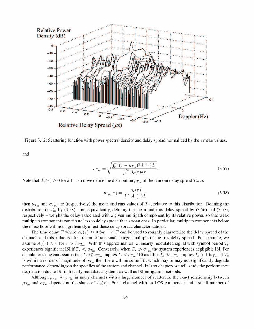
Figure 3.12: Scattering function with power spectral density and delay spread normalized by their mean values.

and

σTm =

√

∫∞0 (τ − µTm)2Ac(τ)dτ

∫∞0 Ac(τ)dτ

. (3.57)

Note that Ac(τ) ≥ 0 for all τ , so if we define the distribution pTm of the random delay spread Tm as

pTm(τ) =Ac(τ)

∫∞0 Ac(τ)dτ

(3.58)

then µTm and σTm are (respectively) the mean and rms values of Tm, relative to this distribution. Defining the

distribution of Tm by (3.58) – or, equivalently, defining the mean and rms delay spread by (3.56) and (3.57),

respectively – weighs the delay associated with a given multipath component by its relative power, so that weak

multipath components contribute less to delay spread than strong ones. In particular, multipath components below

the noise floor will not significantly affect these delay spread characterizations.

The time delay T where Ac(τ) ≈ 0 for τ ≥ T can be used to roughly characterize the delay spread of the

channel, and this value is often taken to be a small integer multiple of the rms delay spread. For example, we

assume Ac(τ) ≈ 0 for τ > 3σTm . With this approximation, a linearly modulated signal with symbol period Tsexperiences significant ISI if Ts � σTm . Conversely, when Ts � σTm the system experiences negligible ISI. For

calculations one can assume that Ts � σTm implies Ts < σTm/10 and that Ts � σTm implies Ts > 10σTm. If Tsis within an order of magnitude of σTm then there will be some ISI, which may or may not significantly degrade

performance, depending on the specifics of the system and channel. In later chapters we will study the performance

degradation due to ISI in linearly modulated systems as well as ISI mitigation methods.

Although µTm ≈ σTm in many channels with a large number of scatterers, the exact relationship between

µTm and σTm depends on the shape of Ac(τ). For a channel with no LOS component and a small number of

95

multipath components with approximately the same large delay, µTm � σTm . In this case the large value of µTm

is a misleading metric of delay spread, since in fact all copies of the transmitted signal arrive at roughly the same

time and the demodulator would synchronize to this common delay. It is typically assumed that the synchronizer

locks to the multipath component at approximately the mean delay, in which case rms delay spread characterizes

the time spreading of the channel.

Example 3.11: The power delay profile is often modeled as having a one-sided exponential distribution:

Ac(τ) =1

Tme−τ/Tm, τ ≥ 0.

Show that the average delay spread (3.56) is µTm = Tm and find the rms delay spread (3.57).

Solution: It is easily shown that Ac(τ) integrates to unity. The average delay spread is thus given by

µTm =1

Tm

∫ ∞

0τe−τ/Tmdτ = Tm,

and the rms delay spread is

σTm =

√

1

Tm

∫ ∞

0

τ2e−τ/Tmdτ − µ2Tm

= 2Tm − Tm = Tm.

Thus, the average and rms delay spread are the same for exponentially distributed power delay profiles.

Example 3.12: Consider a wideband channel with multipath intensity profile

Ac(τ) =

{

e−τ/.00001 0 ≤ τ ≤ 20 µs,

0 else.

Find the mean and rms delay spreads of the channel and find the maximum symbol rate such that a linearly

modulated signal transmitted through this channel does not experience ISI.

Solution: The average delay spread is

µTm =

∫ 20·10−6

0 τe−τ/.00001dτ∫ 20·10−6

0 e−τ/.00001dτ= 6.87 µs.

The rms delay spread is

σTm =

√

√

√

√

∫ 20·10−6

0 (τ − µTm)2e−τ/.00001dτ∫ 20·10−6

0 e−τ/.00001dτ= 5.25 µs.

We see in this example that the mean delay spread is roughly equal to its rms value. To avoid ISI we require linear

modulation to have a symbol period Ts that is large relative to σTm . Taking this to mean that Ts > 10σTm yields

a symbol period of Ts = 52.5 µs or a symbol rate of Rs = 1/Ts = 19.04 kilosymbols per second. This is a

highly constrained symbol rate for many wireless systems. Specifically, for binary modulations where the symbol

96

rate equals the data rate (bits per second, or bps), voice requires on the order of 32 kbps and data has orders of

magnitude higher rates, with some systems operating at Gbps data rates.

3.3.3 Coherence Bandwidth

We can also characterize the time-varying multipath channel in the frequency domain by taking the Fourier trans-

form of c(τ, t) with respect to τ . Specifically, define the random process

C(f ; t) =

∫ ∞

−∞

c(τ ; t)e−j2πfτdτ. (3.59)

Because c(τ ; t) is a complex zero-mean Gaussian random variable in t, the Fourier transform in (3.59) represents

the sum9 of complex zero-mean Gaussian random processes; hence C(f ; t) is also a zero-mean Gaussian random

process that is completely characterized by its autocorrelation. Since c(τ ; t) is WSS, its integral C(f ; t) is also.

Thus, the autocorrelation of (3.59) is given by

AC(f1, f2;4t) = E[C∗(f1; t)C(f2; t+ 4t)]. (3.60)

We can simplify AC(f1, f2;4t) as follows:

AC(f1, f2;4t) = E

[∫ ∞

−∞c∗(τ1; t)e

j2πf1τ 1dτ1

∫ ∞

−∞c(τ2; t+ 4t)e−j2πf2τ 2dτ2

]

=

∫ ∞

−∞

∫ ∞

−∞

E[c∗(τ1; t)c(τ2; t+ 4t)]ej2πf1τ 1e−j2πf2τ 2dτ1dτ2

=

∫ ∞

−∞Ac(τ, 4t)e−j2π(f2−f1)τdτ

= AC(4f ;4t), (3.61)

where 4f = f2 − f1 and the third equality follows from the WSS and US properties of c(τ ; t). Thus, the

autocorrelation of C(f ; t) in frequency depends only on the frequency difference 4f . The function AC(4f ;4t)can be measured in practice by transmitting a pair of sinusoids through the channel that are separated in frequency

by 4f and then calculating their cross-correlation at the receiver for the time separation 4t.If we define AC(4f) , AC(4f ; 0) then, by (3.61),

AC(4f) =

∫ ∞

−∞Ac(τ)e

−j2π4fτdτ. (3.62)

Thus AC(4f) is the Fourier transform of the power delay profile. Because AC(4f) = E[C∗(f ; t)C(f +4f ; t)]

is an autocorrelation, it follows that the channel response is approximately independent at frequency separations

4f where AC(4f) ≈ 0. The frequency Bc where AC(4f) ≈ 0 for all 4f > Bc is called the coherence

bandwidth of the channel. By the Fourier transform relationship between Ac(τ) and AC(4f), if Ac(τ) ≈ 0 for

τ > T then AC(4f) ≈ 0 for 4f > 1/T . Hence, the minimum frequency separation Bc for which the channel

response is roughly independent is Bc ≈ 1/T , where T is typically taken to be the rms delay spread σTm of

Ac(τ). A more general approximation is Bc ≈ k/σTm , where k depends on the shape of Ac(τ) and the precise

specification of coherence bandwidth. For example, Lee [22] has shown that Bc ≈ .02/σTm approximates the

9We can express the integral as a limit of a discrete sum.

97

range of frequencies over which channel correlation exceeds 0.9 whereas Bc ≈ .2/σTm approximates the range of

frequencies over which this correlation exceeds 0.5.

In general, if we are transmitting a narrowband signal with bandwidth B � Bc, then fading across the entire

signal bandwidth is highly correlated; that is, the fading is roughly equal across the entire signal bandwidth. This is

usually referred to as flat fading. On the other hand, if the signal bandwidth B � Bc, then the channel amplitude

values at frequencies separated by more than the coherence bandwidth are roughly independent. Thus, the channel

amplitude varies widely across the signal bandwidth. In this case the fading is called frequency selective. If

B ≈ Bc then channel behavior is somewhere between flat and frequency-selective fading. Note that in linear

modulation the signal bandwidth B is inversely proportional to the symbol time Ts, so flat fading corresponds to

Ts ≈ 1/B � 1/Bc ≈ σTm – that is, the case where the channel experiences negligible ISI. Frequency-selective

fading corresponds to Ts ≈ 1/B � 1/Bc = σTm , the case where the linearly modulated signal experiences

significant ISI. Wideband signaling formats that reduce ISI, such as multicarrier modulation and spread spectrum,

still experience frequency-selective fading across their entire signal bandwidth; this degrades performance, as will

be discussed in Chapters 12 and 13.

We illustrate the power delay profileAc(τ) and its Fourier transformAC(4f) in Figure 3.13. This figure also

shows two signal spectra superimposed on AC(4f) : a narrowband signal with bandwidth much less than Bc, and

a wideband signal with bandwidth much greater thanBc. We see that the autocorrelationAC(4f) is flat across the

bandwidth of the narrowband signal, so this signal will experience flat fading or (equivalently) negligible ISI. The

autocorrelation AC(4f) goes to zero within the bandwidth of the wideband signal, which means that fading will

be independent across different parts of the signal bandwidth; hence fading is frequency selective, and a linearly

modulated signal transmitted through this channel will experience significant ISI.

Figure 3.13: Power delay profile, rms delay spread, and coherence bandwidth.

Example 3.13: Consider an indoor channel with σTm = 30 ns and a large macrocell channel with σTm = 300

ns. Find the maximum symbol rate Rs = 1/Ts for these environments such that a linearly modulated signal

transmitted through them experiences negligible ISI.

Solution: We assume that negligible ISI requires Ts � σTm (i.e., Ts ≥ 10σTm). This translates into a symbol

rate of Rs = 1/Ts ≤ .1/σTm. For σTm = 30 ns this yields Rs ≤ 3.33 Mbps and for σTm = 300 nsthis yields

Rs ≤ 333 Kbps. Note that high-performance wireless systems today can support Gbps data rates indoors and

out. To maintain these data rates for a linearly modulated signal without severe performance degradation by ISI,

some form of ISI mitigation is needed. Moreover, ISI is less severe in indoor than in outdoor systems owing to

the former’s lower delay spread values, which is why indoor systems tend to have higher data rates than outdoor

systems.

98

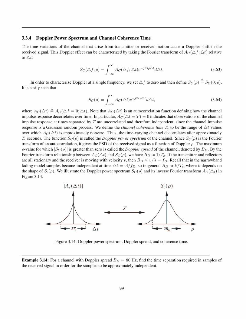
3.3.4 Doppler Power Spectrum and Channel Coherence Time

The time variations of the channel that arise from transmitter or receiver motion cause a Doppler shift in the

received signal. This Doppler effect can be characterized by taking the Fourier transform of AC(4f ;4t) relative

to 4t:

SC(4f ; ρ) =

∫ ∞

−∞AC(4f ;4t)e−j2πρ4td4t. (3.63)

In order to characterize Doppler at a single frequency, we set 4f to zero and then define SC(ρ)4= SC(0; ρ).

It is easily seen that

SC(ρ) =

∫ ∞

−∞AC(4t)e−j2πρ4td4t, (3.64)

where AC(4t) , AC(4f = 0;4t). Note that AC(4t) is an autocorrelation function defining how the channel

impulse response decorrelates over time. In particular,AC(4t = T ) = 0 indicates that observations of the channel

impulse response at times separated by T are uncorrelated and therefore independent, since the channel impulse

response is a Gaussian random process. We define the channel coherence time Tc to be the range of 4t values

over which AC(4t) is approximately nonzero. Thus, the time-varying channel decorrelates after approximately

Tc seconds. The function SC(ρ) is called the Doppler power spectrum of the channel. Since SC(ρ) is the Fourier

transform of an autocorrelation, it gives the PSD of the received signal as a function of Doppler ρ. The maximum

ρ-value for which |SC(ρ)| is greater than zero is called the Doppler spread of the channel, denoted by BD . By the

Fourier transform relationship between AC(4t) and SC(ρ), we have BD ≈ 1/Tc. If the transmitter and reflectors

are all stationary and the receiver is moving with velocity v, then BD ≤ v/λ = fD. Recall that in the narrowband

fading model samples became independent at time 4t = .4/fD, so in general BD ≈ k/Tc, where k depends on

the shape of Sc(ρ). We illustrate the Doppler power spectrum SC(ρ) and its inverse Fourier transform AC(4t) in

Figure 3.14.

Figure 3.14: Doppler power spectrum, Doppler spread, and coherence time.

Example 3.14: For a channel with Doppler spread BD = 80 Hz, find the time separation required in samples of

the received signal in order for the samples to be approximately independent.

99

Solution: The coherence time of the channel is Tc ≈ 1/BD = 1/80, so samples spaced 12.5 ms apart are

approximately uncorrelated. Thus, given the Gaussian properties of the underlying random process, these samples

are approximately independent.

3.3.5 Transforms for Autocorrelation and Scattering Functions

From (3.63) we see that the scattering function Sc(τ ; ρ) defined in (3.55) is the inverse Fourier transform of

SC(4f ; ρ) in the 4f variable. Furthermore Sc(τ ; ρ) and AC(4f ;4t) are related by the double Fourier transform

Sc(τ ; ρ) =

∫ ∞

−∞

∫ ∞

−∞

AC(4f ;4t)e−j2πρ4tej2πτ4fd4t d4f. (3.65)

The relationships among the four functionsAC(4f ;4t), Ac(τ ;4t), SC(4f ; ρ), and Sc(τ ; ρ) are shown in Figure

3.15.

Figure 3.15: Fourier transform relationships.

Empirical measurements of the scattering function for a given channel are often used to approximate the

channel’s delay spread, coherence bandwidth, Doppler spread, and coherence time. The delay spread for a channel

with empirical scattering function Sc(τ ; ρ) is obtained by computing the empirical power delay profileAc(τ) from

Ac(τ, 4t) = F−1ρ [Sc(τ ; ρ)] with 4t = 0 and then computing the mean and rms delay spread from this power

delay profile. The coherence bandwidth can then be approximated as Bc ≈ 1/σTm . Similarly, the Doppler spread

BD is approximated as the range of ρ values over which S(0; ρ) is roughly nonzero, with the coherence time

Tc ≈ 1/BD.

3.4 Discrete-Time Model

Often the time-varying impulse response channel model is too complex for simple analysis. In this case a discrete-

time approximation for the wideband multipath model can be used. This discrete-time model, developed by Turin

in [23], is especially useful in the study of spread-spectrum systems and RAKE receivers (covered in Chapter 13).

This discrete-time model is based on a physical propagation environment consisting of a composition of isolated

point scatterers, as shown in Figure 3.16. In this model, the multipath components are assumed to form subpath

clusters: incoming paths on a given subpath with approximate delay τi are combined, and incoming paths on

100

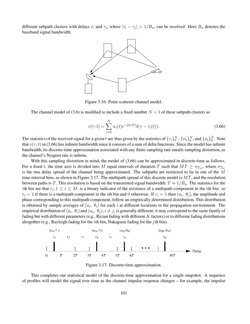
different subpath clusters with delays τi and τj , where |τi − τj| > 1/Bu, can be resolved. Here Bu denotes the

baseband signal bandwidth.

Figure 3.16: Point scatterer channel model.

The channel model of (3.6) is modified to include a fixed number N + 1 of these subpath clusters as

c(τ ; t) =

N∑

i=0

αi(t)e−jφi(t)δ(τ − τi(t)). (3.66)

The statistics of the received signal for a given t are thus given by the statistics of {τi}N0 , {αi}N0 , and {φi}N0 . Note

that c(τ ; t) in (3.66) has infinite bandwidth since it consists of a sum of delta functions. Since the model has infinite

bandwidth, its discrete-time approximation associated with any finite sampling rate entails sampling distortion, as

the channel’s Nyquist rate is infinite.

With this sampling distortion in mind, the model of (3.66) can be approximated in discrete-time as follows.

For a fixed t, the time axis is divided into M equal intervals of duration T such that MT ≥ σTm , where σTm

is the rms delay spread of the channel being approximated. The subpaths are restricted to lie in one of the M

time-interval bins, as shown in Figure 3.17. The multipath spread of this discrete model is MT , and the resolution

between paths is T . This resolution is based on the transmitted signal bandwidth: T ≈ 1/Bu. The statistics for the

ith bin are that ri, 1 ≤ i ≤ M, is a binary indicator of the existence of a multipath component in the ith bin: so

ri = 1 if there is a multipath component in the ith bin and 0 otherwise. If ri = 1 then (ai, θi), the amplitude and

phase corresponding to this multipath component, follow an empirically determined distribution. This distribution

is obtained by sample averages of (ai, θi) for each i at different locations in the propagation environment. The

empirical distribution of (ai, θi) and (aj, θj), i 6= j, is generally different; it may correspond to the same family of

fading but with different parameters (e.g., Rician fading with differentK factors) or to different fading distributions

altogether (e.g., Rayleigh fading for the ith bin, Nakagami fading for the jth bin).

Figure 3.17: Discrete-time approximation.

This completes our statistical model of the discrete-time approximation for a single snapshot. A sequence

of profiles will model the signal over time as the channel impulse response changes – for example, the impulse

101

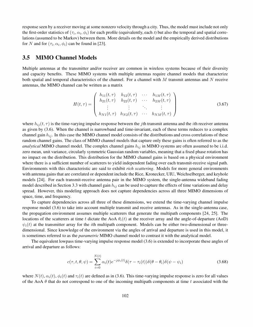
response seen by a receiver moving at some nonzero velocity through a city. Thus, the model must include not only

the first-order statistics of (τi, αi, φi) for each profile (equivalently, each t) but also the temporal and spatial corre-

lations (assumed to be Markov) between them. More details on the model and the empirically derived distributions

for N and for (τi, αi, φi) can be found in [23].

3.5 MIMO Channel Models

Multiple antennas at the transmitter and/or receiver are common in wireless systems because of their diversity

and capacity benefits. These MIMO systems with multiple antennas require channel models that characterize

both spatial and temporal characteristics of the channel. For a channel with M transmit antennas and N receive

antennas, the MIMO channel can be written as a matrix

H(t, τ) =

h11(t, τ) h12(t, τ) · · · h1M (t, τ)h21(t, τ) h22(t, τ) · · · h2M (t, τ)

......

. . ....

hN1(t, τ) hN2(t, τ) · · · hNM (t, τ)

(3.67)

where hij(t, τ) is the time-varying impulse response between the jth transmit antenna and the ith receiver antenna

as given by (3.6). When the channel is narrowband and time-invariant, each of these terms reduces to a complex

channel gain hij . In this case the MIMO channel model consists of the distributions and cross correlations of these

random channel gains. The class of MIMO channel models that capture only these gains is often referred to as the

analytical MIMO channel model. The complex channel gains hij in MIMO systems are often assumed to be i.i.d.

zero mean, unit variance, circularly symmetric Gaussian random variables, meaning that a fixed phase rotation has

no impact on the distribution. This distribution for the MIMO channel gains is based on a physical environment

where there is a sufficient number of scatterers to yield independent fading over each transmit-receive signal path.

Environments with this characteristic are said to exhibit rich scattering. Models for more general environments

with antenna gains that are correlated or dependent include the Rice, Kronecker, UIU, Weichselberger, and keyhole

models [24]. For each transmit-receive antenna pair in the MIMO system, the single-antenna wideband fading

model described in Section 3.3 with channel gain hij can be used to capture the effects of time variations and delay

spread. However, this modeling approach does not capture dependencies across all three MIMO dimensions of

space, time, and frequency.

To capture dependencies across all three of these dimensions, we extend the time-varying channel impulse

response model (3.6) to take into account multiple transmit and receive antennas. As in the single-antenna case,

the propagation environment assumes multiple scatterers that generate the multipath components [24, 25]. The

locations of the scatterers at time t dictate the AoA θi(t) at the receiver array and the angle-of-departure (AoD)

ψi(t) at the transmitter array for the ith multipath component. Models can be either two-dimensional or three-

dimensional. Since knowledge of the environment via the angles of arrival and departure is used in this model, it

is sometimes referred to as the parametric MIMO channel model to contrast it with the analytical model.

The equivalent lowpass time-varying impulse response model (3.6) is extended to incorporate these angles of

arrival and departure as follows:

c(τ, t, θ, ψ) =

N(t)∑

i=0

αi(t)e−jφi(t)δ(τ − τi(t))δ(θ − θi)δ(ψ− ψi) (3.68)

where N (t), αi(t), φi(t) and τi(t) are defined as in (3.6). This time-varying impulse response is zero for all values

of the AoA θ that do not correspond to one of the incoming multipath components at time t associated with the

102

physical environment, and similarly for all values of the AoD ψ. In three dimensions the angles of arrival and

departure of each multipath component depends on the elevation and azimuth angles, the polarization of antenna

elements, as well as the scatterer locations. Survey papers on such 3-D channel models include [26, 27].

103

Chapter 3 Problems

1. Consider a two-ray channel consisting of a direct ray plus a ground-reflected ray where the transmitter is a

fixed base station at height h and the receiver is mounted on a truck (also at height h). The truck starts next to

the base station and moves away at velocity v. Assume signal attenuation on each path follows a free-space

path loss model. Find the time-varying channel impulse at the receiver for transmitter-receiver separation

d = vt sufficiently large for the length of the reflected path to be approximated by x + x′ ≈ d + 2h2/d.

Assume a carrier frequency f = 2 GHz, unit gain antennas at the transmitter and receiver, and reflection

coefficient R = −1.

2. Find a formula for the multipath delay spread Tm for a two-ray channel model. Find a simplified formula

when the transmitter-receiver separation is relatively large. Compute Tm for ht = 10 m, hr = 4 m, and

d = 100 m.

3. Consider a time-invariant indoor wireless channel with LOS component at delay 23 nsec, a multipath com-

ponent at delay 48 ns, and another multipath component at delay 67 ns. Find the delay spread assuming the

demodulator synchronizes to the LOS component. Repeat assuming that the demodulator synchronizes to

the first multipath component.

4. Show that the minimum value of fcτi for a system at fc = 1 GHz with a fixed transmitter and a receiver

separated by more than 10 m from the transmitter is much greater than 1.

5. Prove that forX and Y independent zero-mean Gaussian random variables with variance σ2,Z =√X2 + Y 2

is Rayleigh-distributed and Z2 is exponentially-distributed.

6. Assume a Rayleigh fading channel with average signal power 2σ2 = −80 dBm. What is the power outage

probability of this channel relative to the threshold Po = −95 dBm? How about Po = −90 dBm?

7. Suppose we have an application that requires a power outage probability of .01 for the threshold Po = −80

dBm, For Rayleigh fading, what value of the average signal power is required?

8. Assume a Rician fading channel with 2σ2 = −80 dBm and a target power of Po = −80 dBm. Find the

outage probability assuming that the LOS component has average power s2 = −80 dBm.

9. This problem illustrates that the tails of the Ricean distribution can be quite different than its Nakagami

approximation. Plot the cumulative distribution function (CDF) of the Ricean distribution for K = 1, 5, 10

and the corresponding Nakagami distribution with m = (K + 1)2/(2K + 1). In general, does the Ricean

distribution or its Nakagami approximation have a larger outage probability p(γ < x) for x large?

10. The em Generalized Two Ray (GTR) fading model, proposed in [28], is a generalization of the Rayleigh and

Rician fading models. In this model there are two dominant signal components as well as many lower-power

multipath components. More precisely, the received signal Vr can be modeled as

Vr = V1ejφ1 + V2e

jφ2 +X + jY,

where V1 and V2 are non-negative constants, φi and φ2 are i.i.d. and uniformly distributed over [0, 2π], i.e.

φi ∼ U [0, 2π], i = 1, 2, and X and Y are i.i.d. Gauss-distributed random variables with mean zero and

variance σ2. The GTR model thus reduces to the Rician fading model if V1 > 0, V2 = 0 and to the Rayleigh

104

fading model if V1 = V2 = 0. The model is parameterized in terms of K and ∆ where,

K =V 2

1 + V 22

2σ2

∆ =2V1V2

V 21 + V 2

2

(a) Find the range of parameters K and ∆.

(b) Describe the channel model that corresponds to the following GTR parameters:

• K → ∞,∆ → 0

• K → ∞,∆ → 1

• K → 0

• K > 0,∆ → 0

(c) Show that the received signal given that the phase difference between the 2 dominant components is

constant,i.e., φ1 − φ2 = α for a constant α, consists of one dominant component and the multiple

diffuse lower-power multipath components. This implies that the GTR model reduces to the Rician

fading model when the phase difference between the LoS components in constant. Find the parameter

K(α,∆, K) of the equivalent Rician model as a function of α, ∆ and K.

(d) Show that α (mod 2π) ∼ U [0, 2π]. Use this to show that

pGTR(r | K,∆) =1

2π

∫ 2π

0pRice(r | K(α,∆, K))dα,

where pGTR(r | Σ) is the pdf of the received signal amplitude of the GTR channel fading model with

parameters Σ and pRice(r | Σ) is the pdf of the received signal amplitude of the GTR channel fading

model with parameters Σ.

11. In order to improve the performance of cellular systems, multiple base stations can receive the signal trans-

mitted from a given mobile unit and combine these multiple signals either by selecting the strongest one

or summing the signals together, perhaps with some optimized weights. This typically increases SNR and

reduces the effects of shadowing. Combining of signals received from multiple base stations is called macro-

diversity, and in this problem we explore the benefits of this technique. Diversity will be covered in more

detail in Chapter 7.

Consider a mobile at the midpoint between two base stations in a cellular network. The received signals (in

dBW) from the base stations are given by

Pr,1 = W + Z1,

Pr,2 = W + Z2,

where Z1,2 are N (0, σ2) random variables. We define outage with macrodiversity to be the event that both

Pr,1 and Pr,2 fall below a threshould T . The term W is the received signal power while Z1 and Z2 are

independent noise terms.

(a) If Z1 and Z2 are independent, show that the outage probability is given by

Pout = [Q(∆/σ)]2,

where ∆ = W − T is the fade margin at the mobile’s location.

105

(b) Now suppose Z1 and Z2 are correlated in the following way:

Z1 = a Y1 + b Y,

Z2 = a Y2 + b Y,

where Y, Y1, Y2 are independent N (0, σ2) random variables, and a, b are such that a2 + b2 = 1. Show

that

Pout =

∫ ∞

−∞

1√2π

[

Q

(

∆ + byσ

|a|σ

)]2

e−y2/2dy.

(c) Compare the outage probabilities of (b) and (c) for the special case of a = b = 1/√

2, σ = 8 and

∆ = 5 (this will require a numerical integration).

12. The goal of this problem is to develop a Rayleigh fading simulator for a mobile communications channel

using the method based on filtering Gaussian processes based on the in-phase and quadrature PSDs described

in 3.2.1. In this problem you must do the following:

(a) Develop simulation code to generate a signal with Rayleigh fading amplitude over time. Your sample

rate should be at least 1000 samples/sec, the average received envelope should be 1, and your simulation

should be parameterized by the Doppler frequency fD . Matlab is the easiest way to generate this

simulation, but any simulation tool can be used.

(b) Write a description of your simulation that clearly explains how your code generates the fading enve-

lope using a block diagram and any necessary equations.

(c) Provide plots of received amplitude (dB) vs. time for fD = 1, 10, 100 Hz. over 2 seconds.

13. For a Rayleigh fading channel with average power P r = 30 dB and Doppler frequency fD = 10 Hz,

compute the average fade duration for target fade values P0 = 0 dB, P0 = 15 dB, and P0 = 30 dB.

14. Derive a formula for the average length of time a Rayleigh fading process with average power P r stays

above a given target fade value P0. Evaluate this average length of time for P r = 20 dB, P0 = 25 dB, and

fD = 50 Hz and compare with the average fade depth below P0 associated with the same parameters.

15. Assume a Rayleigh fading channel with average power P r = 10 dB and Doppler fD = 80 Hz. We would

like to approximate the channel using a finite state Markov model with eight states and time interval T = 10ms. The regions Rj corresponds to R1 = {γ : −∞ ≤ γ ≤ −10 dB}, R2 = {γ : −10dB ≤ γ ≤ 0 dB},

R3 = {γ : 0dB ≤ γ ≤ 5 dB}, R4 = {γ : 5dB ≤ γ ≤ 10 dB}, R5 = {γ : 10dB ≤ γ ≤ 15 dB},

R6 = {γ : 15dB ≤ γ ≤ 20 dB}, R7 = {γ : 20dB ≤ γ ≤ 30 dB}, R8 = {γ : 30dB ≤ γ ≤ ∞ }. Find the

transition probabilties between each region for this model.

16. Consider the following channel scattering function obtained by sending a 900 MHz sinusoidal input into the

channel:

S(τ, ρ) =

α1δ(τ) ρ = 70Hz.

α2δ(τ − .022µs) ρ = 49.5Hz.

0 else

where α1 and α2 are determined by path loss, shadowing, and multipath fading. Clearly this scattering

function corresponds to a 2-ray model. Assume the transmitter and receiver used to send and receive the

sinusoid are located eight meters above the ground.

(a) Find the distance and velocity between the transmitter and receiver.

106

(b) For the distance computed in part (a), is the path loss as a function of distance proportional to d−2 or

d−4? Hint: use the fact that the channel is based on a 2-ray model.

(c) Does a 30 KHz voice signal transmitted over this channel experience flat or frequency-selective fading?

17. In this problem we examine the narrowband approximation in the two-ray model. Consider the two-ray

model discussed in Chapter 2.4 with reflection coefficient R = −1, free space path loss for each ray and

carrier frequency 2.4 GHz. Both the transmitter and the receiver are 40 m high.

(a) For a separation distance of 20 m, find the impulse response of the equivalent baseband channel in the

time domain. What is the delay spread Tm?

(b) Repeat the computation of the impulse response and delay spread for a separation distance of 2000 m.

(c) Plot the baseband channel output in both the time and frequency domain in each of the above two

channels for channel input sinc(ft) ,sin(πft)πft and f = 20 MHz. Is there ISI in either channel?

Find the coherence bandwidth of the channel in each case and whether this bandwidth implies flat or

frequency selective fading.

18. Consider a wideband channel characterized by the autocorrelation function

Ac(τ,∆t) =

{

sinc(W∆t) 0 ≤ τ ≤ 10µsec.

0 else,

where W = 100Hz and sinc(x) = sin(πx)/(πx).

(a) Does this channel correspond to an indoor channel or an outdoor channel, and why?

(b) Sketch the scattering function of this channel.

(c) Compute the channel’s average delay spread, rms delay spread, and Doppler spread.

(d) Over approximately what range of data rates will a signal transmitted over this channel exhibit frequency-

selective fading?

(e) Would you expect this channel to exhibit Rayleigh or Ricean fading statistics, and why?

(f) Assuming that the channel exhibits Rayleigh fading, what is the average length of time that the signal

power is continuously below its average value.

(g) Assume a system with narrowband binary modulation sent over this channel. Your system has error

correction coding that can correct two simultaneous bit errors. Assume also that you always make an

error if the received signal power is below its average value, and never make an error if this power is

at or above its average value. If the channel is Rayleigh fading then what is the maximum data rate

that can be sent over this channel with error-free transmission, making the approximation that the fade

duration never exceeds twice its average value.

19. Let a scattering function S(τ, ρ) be nonzero over 0 ≤ τ ≤ .1 ms and −.1 ≤ ρ ≤ .1 Hz. Assume that the

power of the scattering function is approximately uniform over the range where it is nonzero.

(a) What are the multipath spread and the Doppler spread of the channel?

(b) Suppose you input to this channel two sinusoids cos(2πf1t) and cos(2πf2t) separated in frequency by

∆f = |f1−f2|. What is the minimum value of ∆f for which the channel response to the first sinusoid

is approximately independent of the channel response to the second sinusoid.

107

(c) For two sinusoidal inputs to the channel u1(t) = sin(2πft) and u2(t) = sin(2πf(t+ ∆t)), find the

minimum value of ∆t for which the channel response to u1(t) is approximately independent of the

channel response to u2(t).

(d) Will this channel exhibit flat fading or frequency-selective fading for a typical voice channel with a 3

KHz bandwidth? How about for a cellular channel with a 30 KHz bandwidth?

20. Consider a MIMO channel H with a time-invariant complex gain hij between the jth transmit antenna and

the ith receive antenna. A MIMO channel is called a keyhole channel when the channel matrix H can be

written as

H = hrh∗t

where ht is an M × 1 vector of i.i.d. zero-mean unit variance complex Gaussian random variables, and hris an N × 1 vector of i.i.d. zero-mean unit variance complex Gaussian random variables. Thus, hij is the

product of two independent complex Gaussian random variables.

(a) Show that the power of hij has a distribution p(x) = 2K0(2√x) where K0 is the modified Bessel

function of the second kind.

(b) Show that the matrix H has rank 1, i.e. show that all of its columns are linearly dependent, and the

same for its rows.

The fact that the matrix H is rank 1 is what gives rise to the name keyhole channel, since the MIMO channel’s

multiple spatial dimensions reduce to a single dimension, as if the signal between the transmit and receive

antenna arrays travels through a keyhole.

108

Bibliography

[1] T. S. Rappaport, Wireless Communications – Principles and Practice, 2nd ed., Prentice-Hall, Englewood

Cliffs, NJ, 2001.

[2] D. Parsons, The Mobile Radio Propagation Channel, Wiley, New York, 1994.

[3] R. S. Kennedy, Fading Dispersive Communication Channels, Wiley, New York, 1969.

[4] R. H. Clarke, “A statistical theory of mobile radio reception,” Bell System Tech. J., pp. 957–1000, July/August

1968.

[5] W. C. Jakes, Jr., Microwave Mobile Communications, Wiley, New York, 1974.

[6] M. K. Simon and M.-S. Alouini, Digital Communication over Fading Channels: A Unified Approach to

Performance Analysis, 2nd Ed., Wiley, New York, 2004.

[7] G. L. Stuber, Principles of Mobile Communications, 2nd ed., Kluwer, Dordrecht, 2001.

[8] J. Zhang, C. Pan, F. Pei, G. Liu, and X. Cheng, Three-dimensional fading channel models: a survey of

elevation angle research, IEEE Commun. Mag., vol. 52, no. 6, pp. 218226, 2014.

[9] M. Patzold, Mobile Fading Channels, Wiley, New York, 2002.

[10] J. Cavers, Mobile Channel Characteristics, Springer 2000.

[11] S. O. Rice, “Mathematical analysis of random noise,” Bell System Tech. J., pp. 282–333, July 1944, and pp.

46–156, January 1945.

[12] F. Babich, G. Lombardi, and E. Valentinuzzi, “Variable order Markov modeling for LEO mobile satellite

channels,” Elec. Lett., pp. 621–3, April 1999.

[13] A. M. Chen and R. R. Rao, “On tractable wireless channel models,” Proc. Intemat. Sympos. Pers., Indoor,

Mobile Radio Commun., pp. 825–30, September 1998.

[14] H. S. Wang and N. Moayeri, “Finite-state Markov channel – A useful model for radio communication chan-

nels,” IEEE Trans. Veh. Tech., pp. 163–71, February 1995.

[15] C. C. Tan and N. C. Beaulieu, “On first-order Markov modeling for the Rayleigh fading channel,” IEEE

Trans. Commun., pp. 2032–40, December 2000.

[16] C. Pimentel and I. F. Blake, “Modeling burst channels using partitioned Fritchman’s Markov models,” IEEE

Trans. Veh. Tech., pp. 885–99, August 1998.

109

[17] Y. L. Guan and L. F. Tumer, “Generalised FSMC model for radio channels with correlated fading,” IEE Proc.

Commun., pp. 133–7, April 1999.

[18] M. Chu and W. Stark, “Effect of mobile velocity on communications in fading channels,” IEEE Trans. Veh.

Tech., pp. 202–10, January 2000.

[19] C. Komninakis and R. D. Wesel, “Pilot-aided joint data and channel estimation in flat correlated fading,”

Proc. IEEE Globecom Conf., pp. 2534–9, November 1999.

[20] M. Peleg, S. Shamai (Shitz), and S. Galan, “Iterative decoding for coded noncoherent MPSK communications

over phase-noisy AWGN channels,” IEE Proc. Commun., pp. 87–95, April 2000.

[21] P. A. Bello, “Characterization of randomly time-variant linear channels,” IEEE Trans. Commun. Syst., pp.

360–93, December 1963.

[22] W. C. Y. Lee, Mobile Cellular Telecommunications Systems, McGraw-Hill, New York, 1989.

[23] G. L. Turin, “Introduction to spread spectrum antimultipath techniques and their application to urban digital

radio,” Proc. IEEE, pp. 328–53, March 1980.

[24] R. W. Heath and A. Lozano, Foundations of MIMO Communication, Cambridge University Press, 2019.

[25] R. Ertel, P. Cardieri, K. W. Sowerby, T. S. Rappaport, and J. H. Reed, “Overview of spatial channel models

for antenna array communication systems,” IEEE Personal Communications Magazine., pp. 10–22, February

1998.

[26] U. Karabulut, A. Awada, I. Viering, M. Simsek, and G. P. Fettweis, Spatial and Temporal Channel Character-

istics of 5G 3D Channel Model with Beamforming for User Mobility Investigations IEEE Communications

Magazine, Special Issue on Channel Models and Measurements for 5G, Dec. 2018.

[27] J. Zhang, C. Pan, F. Pei, G. Liu, and X. Cheng, Three-dimensional fading channel models: a survey of

elevation angle research, IEEE Communications Magazine, June 2014.

[28] G. D. Durgin, T. S. Rappaport, D. A. de Wolf, “New analytical models and probability density functions for

fading in wireless communications, IEEE Transactions on Communications, vol. 50, no. 6, pp. 1005-1015,

Jun. 2002.

110

Chapter 4

Capacity of Wireless Channels

The growing demand for wireless communication makes it important to determine the capacity limits of the under-

lying channels for these systems. These capacity limits dictate the maximum data rates that can be transmitted over

wireless channels with asymptotically small error probability, assuming no constraints on delay or complexity of

the encoder and decoder. The mathematical theory of communication underlying channel capacity was pioneered

by Claude Shannon in the late 1940s. This theory is based on the notion of mutual information between the in-

put and output of a channel [1, 2, 3]. In particular, Shannon defined channel capacity as the channel’s mutual

information maximized over all possible input distributions. The significance of this mathematical construct was

Shannon’s coding theorem and its converse. The coding theorem proved that a code did exist that could achieve

a data rate close to capacity with negligible probability of error. The converse proved that any data rate higher

than capacity could not be achieved without an error probability bounded away from zero. Shannon’s ideas were

quite revolutionary at the time: the high data rates he predicted for telephone channels, and his notion that coding

could reduce error probability without reducing data rate or causing bandwidth expansion. In time, sophisticated

modulation and coding technology validated Shannon’s theory and so, on telephone lines today, we achieve data

rates very close to Shannon capacity with very low probability of error. These sophisticated modulation and coding

strategies are treated in Chapters 5 and 8, respectively.

In this chapter we examine the capacity of a single-user wireless channel where transmitter and/or receiver

have a single antenna. The capacity of single-user MIMO systems where the transmitter and receiver both have

multiple antennas is treated in Chapter 10 and that of multiuser systems in Chapter 14. We will discuss capacity

for channels that are both time invariant and time varying. We first look at the well-known formula for capacity

of a time-invariant additive white Gaussian noise (AWGN) channel and then consider capacity of time-varying

flat fading channels. Unlike the AWGN case, here the capacity of a flat fading channel is not given by a single

formula because capacity depends on what is known about the time-varying channel at the transmitter and/or re-

ceiver. Moreover, for different channel information assumptions there are different definitions of channel capacity,

depending on whether capacity characterizes the maximum rate averaged over all fading states or the maximum

constant rate that can be maintained in all fading states (with or without some probability of outage).

We will first consider flat fading channel capacity where only the fading distribution is known at the transmitter

and receiver. Capacity under this assumption is typically difficult to determine and is only known in a few special

cases. Next we consider capacity when the channel fade level is known at the receiver only (via receiver estimation)

or when the channel fade level is known at both the transmitter and the receiver (via receiver estimation and

transmitter feedback). We will see that the fading channel capacity with channel fade level information at both

the transmitter and receiver is achieved when the transmitter adapts its power, data rate, and coding scheme to the

channel variation. The optimal power allocation in this case is a “water-filling” in time, where power and data rate

are increased when channel conditions are favorable and decreased when channel conditions are not favorable.

111

We will also treat capacity of frequency-selective fading channels. For time-invariant frequency-selective

channels the capacity is known and is achieved with an optimal power allocation that water-fills over frequency in-

stead of time. The capacity of a time-varying frequency-selective fading channel is unknown in general. However,

this channel can be approximated as a set of independent parallel flat fading channels whose capacity is the sum of

capacities on each channel with power optimally allocated among the channels. The capacity of such a channel is

known and the capacity-achieving power allocation water-fills over both time and frequency.

We will consider only discrete-time systems in this chapter. Most continuous-time systems can be converted

to discrete-time systems via sampling, and then the same capacity results hold. However, care must be taken in

choosing the appropriate sampling rate for this conversion, since time variations in the channel may increase the

sampling rate required to preserve channel capacity [4].

4.1 Capacity in AWGN

Consider a discrete-time AWGN channel with channel input/out relationship y[i] = x[i] + n[i], where x[i] is

the channel input at time i, y[i] is the corresponding channel output, and n[i] is a white Gaussian noise random

process. Assume a channel bandwidthB and received signal power P . The received signal-to-noise ratio (SNR) –

the power in x[i] divided by the power in n[i] – is constant and given by γ = P/(N0B), where N0/2 is the power

spectral density (PSD) of the noise. The capacity of this channel is given by Shannon’s well-known formula [1]:

C = B log2(1 + γ), (4.1)

where the capacity units are bits per second (bps). Shannon’s coding theorem proves that a code exists that achieves

data rates arbitrarily close to capacity with arbitrarily small probability of bit error. The converse theorem shows

that any code with rate R > C has a probability of error bounded away from zero.

Shannon capacity for AWGN channels provides interesting insights along the asymptotic regimes of band-

width and power. In particular, it is easily shown that

limB→∞

B log2

(

1 +P

N0B

)

= log2(e)P

N0. (4.2)

This regime is called the large bandwidth regime for capacity. Interestingly, in this regime the capacity no longer

depends on the bandwidth B. That is because there is not sufficient power to spread over the large amount of

bandwidth available, so as the bandwidth grows large, there is diminishing returns in capacity growth. The low

power regime captures a similar scenario, where there is not sufficient power to utilize the available bandwidth. In

particular, using the approximation that log(1 + x) ≈ x for x small yields that, for P small,

B log2

(

1 +P

N0B

)

≈ log2(e)P

N0. (4.3)

Here we also see that capacity no longer depends on the channel bandwidth. Another interesting regime for

capacity is the high power regime, where P grows large. We now consider how capacity scales with bandwidth

in this regime. Using the high-power approximation 1 + P/(N0B) ≈ P/(N0B), we get the following ratio of

AWGN channel capacity C(kB) given bandwidth kB compared with C(B) for any constant k > 1 in the limit of

asymptotically large power:

limP→∞

C(kB)

C(B)= lim

P→∞

kB log2

(

1 + PN0kB

)

B log2

(

1 + PN0B

) ≈ limP→∞

kB log2

(

PN0kB

)

B log2

(

PN0B

) = limP→∞

k[

log2

(

PN0B

)

+ log2(1/k)]

log2

(

PN0B

) = k.

(4.4)

112

Thus, in the high power regime, scaling the bandwidth up by a factor of k leads to the same increase in capacity.

That is because there is sufficient power to fully utilize the capacity of the additional bandwidth.

Shannon’s coding theorem and its converse are proved using the concept of mutual information between the

channel input and output. For a discrete memoryless time-invariant channel with random input x and random

output y, the channel’s mutual information is defined as

I(X ; Y ) =∑

x∈X ,y∈Y

p(x, y) log

(

p(x, y)

p(x)p(y)

)

, (4.5)

where the sum is taken over all possible input and output pairs x ∈ X and y ∈ Y for X and Y the discrete

input and output alphabets. The log function is typically with respect to base 2, in which case the units of mutual

information are bits per second. Mutual information can also be written in terms of the entropy in the channel

output y and conditional output y | x as I(X ; Y ) = H(Y ) − H(Y |X), where H(Y ) = −∑y∈Y p(y) logp(y)and H(Y |X) = −∑x∈X ,y∈Y p(x, y) logp(y | x). Shannon proved that channel capacity equals the mutual

information of the channel maximized over all possible input distributions:

C = maxp(x)

I(X ; Y ) = maxp(x)

∑

x,y

p(x, y) log

(

p(x, y)

p(x)p(y)

)

. (4.6)

For the AWGN channel, the sum in (4.6) becomes an integral over continuous alphabets and the maximizing input

distribution is Gaussian, which results in the channel capacity given by (4.1). For channels with memory, mutual

information and channel capacity are defined relative to input and output sequences xn and yn. More details on

channel capacity, mutual information, the coding theorem, and its converse can be found in [2, 5, 6].

The proofs of the coding theorem and its converse place no constraints on the complexity or delay of the

communication system. Indeed, the capacity-achieving strategy requires a code with an asymptotically large

blocklength to drive the error probability to zero. Such codes require asymptotically large transmission energy

and asymptotically large delay and complexity to decode. Since practical decoders are constrained in delay and

complexity, Shannon capacity is generally used as an upper bound on the data rates that can be achieved under real

system constraints. The exact capacity penalty due to finite blocklength codes was derived in [7] as a function of

blocklength, error probability, and the channel dispersion, which measures the stochastic variability of the channel

relative to a deterministic channel with the same capacity.

At the time that Shannon developed his theory of information, data rates over standard telephone lines were

on the order of 100 bps. Thus, it was believed that Shannon capacity, which predicted speeds of roughly 30 kbps

over the same telephone lines, was not a useful bound for real systems. However, by the 1990s breakthroughs

in hardware, modulation, and coding techniques brought commercial modems very close to the speeds predicted

by Shannon in the 1940s. In fact, modems can exceed this 30-kbps limit on some telephone channels, but that is

because transmission lines today are of better quality than in Shannon’s day and thus have a higher received power

than that used in his initial calculation. Advances in coding techniques over the last few decades include turbo

codes [8], LDPC codes (originally developed by Gallager in the 1960s and rediscovered in the 1990s) [9], lattice

codes [10], and polar codes [11]. All of these codes come within a fraction of a decibel of the Shannon capacity

limit using practical blocklengths. These codes and their performance will be covered in Chapter 8.

Wireless channels typically exhibit flat or frequency-selective fading. In the next two sections we consider ca-

pacity of flat fading and frequency-selective fading channels under different assumptions regarding what is known

about the channel.

Example 4.15: Consider a wireless channel where power falloff with distance follows the formula Pr(d) =

Pt(d0/d)3 for d0 = 10 m. Assume the channel has bandwidth B = 30 kHz and AWGN with noise PSD N0/2,

113

where N0 = 10−9 W/Hz. For a transmit power of 1 W, find the capacity of this channel for a transmit-receive

distance of 100 m and 1 km.

Solution: The received SNR is γ = Pr(d)/(N0B) = .13/(10−9 · 30 · 103) = 33 = 15 dB for d = 100 mand γ = .013/(10−9 · 30 · 103) = .033 = −15 dB for d = 1000 m. The corresponding capacities are C =

B log2(1 + γ) = 30000 log2(1 + 33) = 152.6 kbps for d = 100 m and C = 30000 log2(1 + .033) = 1.4 kbps

for d = 1000 m. Note the significant decrease in capacity at greater distances due to the path-loss exponent of 3,

which greatly reduces received power as distance increases.

Figure 4.1: Flat fading channel and system model.

4.2 Capacity of Flat Fading Channels

4.2.1 Channel and System Model

We assume a discrete-time channel with stationary and ergodic time-varying gain√

g[i], 0 ≤ g[i], and AWGN

n[i], as shown in Figure 4.1. The channel power gain g[i] follows a given distribution p(g); for example, with

Rayleigh fading p(g) is exponential. We assume that g[i] is independent of the channel input. The channel gain

g[i] can change at each time i, either as an independent and identically distributed (i.i.d.) process or with some

correlation over time. In a block fading channel, g[i] is constant over some blocklength T , after which time g[i]

changes to a new independent value based on the distribution p(g). Let P denote the average transmit signal

power, N0/2 the noise PSD of n[i], and B the received signal bandwidth. The instantaneous received SNR is then

γ[i] = P g[i]/(N0B), 0 ≤ γ[i] < ∞, and its expected value over all time is γ = P g/(N0B). Since P /(N0B) is

a constant, the distribution of g[i] determines the distribution of γ[i] and vice versa.

The system model is also shown in Figure 4.1, where an input message w is sent from the transmitter to the

receiver, which reconstructs an estimate w of the transmitted message w from the received signal. The message

is encoded into the codeword x, which is transmitted over the time-varying channel as x[i] at time i. The channel

gain g[i], also called the channel side information (CSI), changes during the transmission of the codeword.

The capacity of this channel depends on what is known about g[i] at the transmitter and receiver. We will

consider three different scenarios regarding this knowledge as follows.

1. Channel distribution information (CDI): The distribution of g[i] is known to the transmitter and receiver.

2. Receiver CSI : The value of g[i] is known to the receiver at time i, and both the transmitter and receiver

know the distribution of g[i].

3. Transmitter and receiver CSI: The value of g[i] is known to the transmitter and receiver at time i, and both

the transmitter and receiver know the distribution of g[i].

Transmitter and receiver CSI allow the transmitter to adapt both its power and rate to the channel gain at time i,leading to the highest capacity of the three scenarios. Note that since the instantaneous SNR γ[i] just g[i] multipled

114

by the constant P /(N0B), known CSI or CDI about g[i] yields the same information about γ[i]. Capacity for

time-varying channels under assumptions other than these three are discussed in [12, 13].

4.2.2 Channel Distribution Information Known

We first consider the case where the channel gain distribution p(g) or, equivalently, the distribution of SNR p(γ)is known to the transmitter and receiver. For i.i.d. fading the capacity is given by (4.6), but solving for the

capacity-achieving input distribution (i.e., the distribution achieving the maximum in that equation) can be quite

complicated depending on the nature of the fading distribution. Moreover, fading correlation introduces channel

memory, in which case the capacity-achieving input distribution is found by optimizing over input blocks, and this

makes finding the solution even more difficult. For these reasons, finding the capacity-achieving input distribu-

tion and corresponding capacity of fading channels under CDI remains an open problem for almost all channel

distributions.

The capacity-achieving input distributionand corresponding fading channel capacity under CDI are known for

two specific models of interest: i.i.d. Rayleigh fading channels and finite-state Markov channels. In i.i.d. Rayleigh

fading, the channel power gain is exponentially distributed and changes independently with each channel use. The

optimal input distribution for this channel was shown in [14] to be discrete with a finite number of mass points, one

of which is located at zero. This optimal distribution and its corresponding capacity must be found numerically.

The lack of closed-form solutions for capacity or the optimal input distribution is somewhat surprising given that

the fading follows the most common fading distribution and has no correlation structure. For flat fading channels

that are not necessarily Rayleigh or i.i.d., upper and lower bounds on capacity have been determined in [15], and

these bounds are tight at high SNRs.

Approximating Rayleigh fading channels via FSMCs was discussed in Chapter 3.2.4. This model approxi-

mates the fading correlation as a Markov process. Although the Markov nature of the fading dictates that the fading

at a given time depends only on fading at the previous time sample, it turns out that the receiver must decode all

past channel outputs jointly with the current output for optimal (i.e. capacity-achieving) decoding. This signifi-

cantly complicates capacity analysis. The capacity of FSMCs has been derived for i.i.d. inputs in [16, 17] and for

general inputs in [18]. Capacity of the FSMC depends on the limiting distribution of the channel conditioned on

all past inputs and outputs, which can be computed recursively. As with the i.i.d. Rayleigh fading channel, the

final result and complexity of the capacity analysis are high for this relatively simple fading model. This shows the

difficulty of obtaining the capacity and related design insights on channels when only CDI is available.

4.2.3 Channel Side Information at Receiver

We now consider the case where the CSI g[i] is known to the receiver at time i. Equivalently, γ[i] is known to

the receiver at time i. We also assume that both the transmitter and receiver know the distribution of g[i]. In this

case there are two channel capacity definitions that are relevant to system design: Shannon capacity, also called

ergodic capacity, and capacity with outage. As for the AWGN channel, Shannon capacity defines the maximum

data rate that can be sent over the channel with asymptotically small error probability. Note that for Shannon

capacity the rate transmitted over the channel is constant: the transmitter cannot adapt its transmission strategy

relative to the CSI. Thus, poor channel states typically reduce Shannon capacity because the transmission strategy

must incorporate the effect of these poor states. An alternate capacity definition for fading channels with receiver

CSI is capacity with outage. This is defined as the maximum rate that can be transmitted over a channel with an

outage probability corresponding to the probability that the transmission cannot be decoded with negligible error

probability. The basic premise of capacity with outage is that a high data rate can be sent over the channel and

decoded correctly except when the channel is in a slow deep fade. By allowing the system to lose some data in the

event of such deep fades, a higher data rate can be maintained than if all data must be received correctly regardless

115

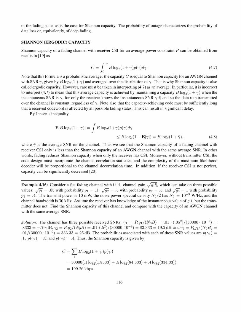
of the fading state, as is the case for Shannon capacity. The probability of outage characterizes the probability of

data loss or, equivalently, of deep fading.

SHANNON (ERGODIC) CAPACITY

Shannon capacity of a fading channel with receiver CSI for an average power constraint P can be obtained from

results in [19] as

C =

∫ ∞

0B log2(1 + γ)p(γ)dγ. (4.7)

Note that this formula is a probabilistic average: the capacityC is equal to Shannon capacity for an AWGN channel

with SNR γ , given by B log2(1+ γ) and averaged over the distribution of γ . That is why Shannon capacity is also

called ergodic capacity. However, care must be taken in interpreting (4.7) as an average. In particular, it is incorrect

to interpret (4.7) to mean that this average capacity is achieved by maintaining a capacity B log2(1 + γ) when the

instantaneous SNR is γ , for only the receiver knows the instantaneous SNR γ[i] and so the data rate transmitted

over the channel is constant, regardless of γ . Note also that the capacity-achieving code must be sufficiently long

that a received codeword is affected by all possible fading states. This can result in significant delay.

By Jensen’s inequality,

E[B log2(1 + γ)] =

∫

B log2(1+γ)p(γ)dγ

≤ B log2(1 + E[γ]) = B log2(1 + γ), (4.8)

where γ is the average SNR on the channel. Thus we see that the Shannon capacity of a fading channel with

receiver CSI only is less than the Shannon capacity of an AWGN channel with the same average SNR. In other

words, fading reduces Shannon capacity when only the receiver has CSI. Moreover, without transmitter CSI, the

code design must incorporate the channel correlation statistics, and the complexity of the maximum likelihood

decoder will be proportional to the channel decorrelation time. In addition, if the receiver CSI is not perfect,

capacity can be significantly decreased [20].

Example 4.16: Consider a flat fading channel with i.i.d. channel gain√

g[i], which can take on three possible

values:√g1 = .05 with probability p1 = .1,

√g2 = .5 with probability p2 = .5, and

√g3 = 1 with probability

p3 = .4. The transmit power is 10 mW, the noise power spectral density N0/2 has N0 = 10−9 W/Hz, and the

channel bandwidth is 30 kHz. Assume the receiver has knowledge of the instantaneous value of g[i] but the trans-

mitter does not. Find the Shannon capacity of this channel and compare with the capacity of an AWGN channel

with the same average SNR.

Solution: The channel has three possible received SNRs: γ1 = Ptg1/(N0B) = .01 · (.052)/(30000 · 10−9) =.8333 = −.79 dB, γ2 = Ptg2/(N0B) = .01·(.52)/(30000·10−9) = 83.333 = 19.2 dB, and γ3 = Ptg3/(N0B) =

.01/(30000 · 10−9) = 333.33 = 25 dB. The probabilities associated with each of these SNR values are p(γ1) =

.1, p(γ2) = .5, and p(γ3) = .4. Thus, the Shannon capacity is given by

C =∑

i

B log2(1 + γi)p(γi)

= 30000(.1 log2(1.8333) + .5 log2(84.333) + .4 log2(334.33))

= 199.26 kbps.

116

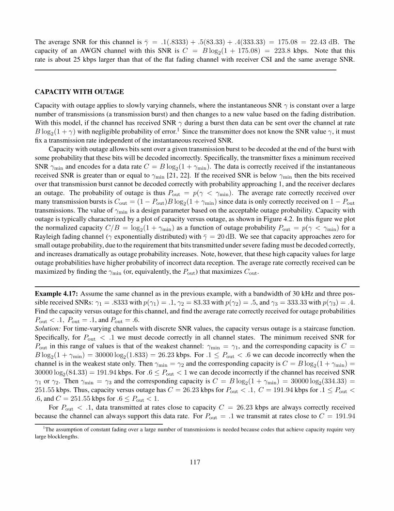
The average SNR for this channel is γ = .1(.8333) + .5(83.33) + .4(333.33) = 175.08 = 22.43 dB. The

capacity of an AWGN channel with this SNR is C = B log2(1 + 175.08) = 223.8 kbps. Note that this

rate is about 25 kbps larger than that of the flat fading channel with receiver CSI and the same average SNR.

CAPACITY WITH OUTAGE

Capacity with outage applies to slowly varying channels, where the instantaneous SNR γ is constant over a large

number of transmissions (a transmission burst) and then changes to a new value based on the fading distribution.

With this model, if the channel has received SNR γ during a burst then data can be sent over the channel at rate

B log2(1 + γ) with negligible probability of error.1 Since the transmitter does not know the SNR value γ , it must

fix a transmission rate independent of the instantaneous received SNR.

Capacity with outage allows bits sent over a given transmission burst to be decoded at the end of the burst with

some probability that these bits will be decoded incorrectly. Specifically, the transmitter fixes a minimum received

SNR γmin and encodes for a data rate C = B log2(1 + γmin). The data is correctly received if the instantaneous

received SNR is greater than or equal to γmin [21, 22]. If the received SNR is below γmin then the bits received

over that transmission burst cannot be decoded correctly with probability approaching 1, and the receiver declares

an outage. The probability of outage is thus Pout = p(γ < γmin). The average rate correctly received over

many transmission bursts is Cout = (1− Pout)B log2(1 + γmin) since data is only correctly received on 1 − Pout

transmissions. The value of γmin is a design parameter based on the acceptable outage probability. Capacity with

outage is typically characterized by a plot of capacity versus outage, as shown in Figure 4.2. In this figure we plot

the normalized capacity C/B = log2(1 + γmin) as a function of outage probability Pout = p(γ < γmin) for a

Rayleigh fading channel (γ exponentially distributed) with γ = 20 dB. We see that capacity approaches zero for

small outage probability, due to the requirement that bits transmitted under severe fading must be decoded correctly,

and increases dramatically as outage probability increases. Note, however, that these high capacity values for large

outage probabilities have higher probability of incorrect data reception. The average rate correctly received can be

maximized by finding the γmin (or, equivalently, the Pout) that maximizes Cout.

Example 4.17: Assume the same channel as in the previous example, with a bandwidth of 30 kHz and three pos-

sible received SNRs: γ1 = .8333 with p(γ1) = .1, γ2 = 83.33 with p(γ2) = .5, and γ3 = 333.33 with p(γ3) = .4.

Find the capacity versus outage for this channel, and find the average rate correctly received for outage probabilities

Pout < .1, Pout = .1, and Pout = .6.

Solution: For time-varying channels with discrete SNR values, the capacity versus outage is a staircase function.

Specifically, for Pout < .1 we must decode correctly in all channel states. The minimum received SNR for

Pout in this range of values is that of the weakest channel: γmin = γ1, and the corresponding capacity is C =

B log2(1 + γmin) = 30000 log2(1.833) = 26.23 kbps. For .1 ≤ Pout < .6 we can decode incorrectly when the

channel is in the weakest state only. Then γmin = γ2 and the corresponding capacity is C = B log2(1 + γmin) =

30000 log2(84.33) = 191.94 kbps. For .6 ≤ Pout < 1 we can decode incorrectly if the channel has received SNR

γ1 or γ2. Then γmin = γ3 and the corresponding capacity is C = B log2(1 + γmin) = 30000 log2(334.33) =

251.55 kbps. Thus, capacity versus outage has C = 26.23 kbps for Pout < .1, C = 191.94 kbps for .1 ≤ Pout <.6, and C = 251.55 kbps for .6 ≤ Pout < 1.

For Pout < .1, data transmitted at rates close to capacity C = 26.23 kbps are always correctly received

because the channel can always support this data rate. For Pout = .1 we transmit at rates close to C = 191.94

1The assumption of constant fading over a large number of transmissions is needed because codes that achieve capacity require very

large blocklengths.

117

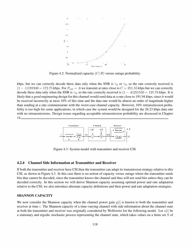
Figure 4.2: Normalized capacity (C/B) versus outage probability.

kbps, but we can correctly decode these data only when the SNR is γ2 or γ3, so the rate correctly received is

(1− .1)191940 = 172.75 kbps. For Pout = .6 we transmit at rates close to C = 251.55 kbps but we can correctly

decode these data only when the SNR is γ3, so the rate correctly received is (1 − .6)251550 = 125.78 kbps. It is

likely that a good engineering design for this channel would send data at a rate close to 191.94 kbps, since it would

be received incorrectly at most 10% of this time and the data rate would be almost an order of magnitude higher

than sending at a rate commensurate with the worst-case channel capacity. However, 10% retransmission proba-

bility is too high for some applications, in which case the system would be designed for the 26.23 kbps data rate

with no retransmissions. Design issues regarding acceptable retransmission probability are discussed in Chapter

14.

Figure 4.3: System model with transmitter and receiver CSI.

4.2.4 Channel Side Information at Transmitter and Receiver

If both the transmitter and receiver have CSI then the transmitter can adapt its transmission strategy relative to this

CSI, as shown in Figure 4.3. In this case there is no notion of capacity versus outage where the transmitter sends

bits that cannot be decoded, since the transmitter knows the channel and thus will not send bits unless they can be

decoded correctly. In this section we will derive Shannon capacity assuming optimal power and rate adaptation

relative to the CSI; we also introduce alternate capacity definitions and their power and rate adaptation strategies.

SHANNON CAPACITY

We now consider the Shannon capacity when the channel power gain g[i] is known to both the transmitter and

receiver at time i. The Shannon capacity of a time-varying channel with side information about the channel state

at both the transmitter and receiver was originally considered by Wolfowitz for the following model. Let s[i] be

a stationary and ergodic stochastic process representing the channel state, which takes values on a finite set S of

118

discrete memoryless channels. Let Cs denote the capacity of a particular channel s ∈ S and let p(s) denote the

probability, or fraction of time, that the channel is in state s. The capacity of this time-varying channel is then

given by Theorem 4.6.1 of [23]:

C =∑

s∈S

Csp(s). (4.9)

We now apply this formula to the system model in Figure 4.3. We know that the capacity of an AWGN

channel with average received SNR γ is Cγ = B log2(1 + γ). Let p(γ) = p(γ[i] = γ) denote the distribution

of the received SNR. By (4.9), the capacity of the fading channel with transmitter and receiver side information is

thus2

C =

∫ ∞

0Cγp(γ)dγ =

∫ ∞

0B log2(1 + γ)p(γ)dγ. (4.10)

We see that, without power adaptation, (4.7) and (4.10) are the same, so transmitter side information does not

increase capacity unless power is also adapted.

Now let us allow the transmit power P (γ) to vary with γ subject to an average power constraint P :

Figure 4.4: Multiplexed coding and decoding.

∫ ∞

0P (γ)p(γ)dγ ≤ P . (4.11)

With this additional constraint, we cannot apply (4.10) directly to obtain the capacity. However, we expect that the

capacity with this average power constraint will be the average capacity given by (4.10) with the power optimally

distributed over time. This motivates our definition of the fading channel capacity with average power constraint

(4.11) as

C = maxP (γ):

R

P (γ)p(γ)dγ=P

∫ ∞

0

B log2(1 +P (γ)γ

P)p(γ)dγ. (4.12)

It is proved in [24] that the capacity given in (4.12) an be achieved and that any rate larger than this capacity

has probability of error bounded away from zero. The main idea behind the proof is a “time diversity” system with

multiplexed input and demultiplexed output, as shown in Figure 4.4. Specifically, we first quantize the range of

fading values to a finite set {γj : 1 ≤ j ≤ N}. For each γj , we design an encoder–decoder pair for an AWGN

channel with SNR γj . The input xj for encoder γj has average power P (γj) and data rate Rj = Cj , where Cjis the capacity of a time-invariant AWGN channel with received SNR P (γj)γj/P . These encoder–decoder pairs

correspond to a set of input and output ports associated with each γj . When γ[i] ≈ γj , the corresponding pair of

ports are connected through the channel. The codewords associated with each γj are thus multiplexed together for

transmission and then demultiplexed at the channel output. This effectively reduces the time-varying channel to a

set of time-invariant channels in parallel, where the jth channel operates only when γ[i] ≈ γj . The average rate on

2Wolfowitz’s result was for γ ranging over a finite set, but it can be extended to infinite sets [24].

119

the channel is just the sum of rates associated with each of the γj channels weighted by p(γj), the percentage of

time that the channel SNR equals γj. This yields the average capacity formula (4.12).

To find the optimal power allocation P (γ), we form the Lagrangian

J(P (γ)) =

∫ ∞

0B log2

(

1 +γP (γ)

P

)

p(γ)dγ− λ

∫ ∞

0P (γ)p(γ)dγ. (4.13)

Next we differentiate the Lagrangian and set the derivative equal to zero:

∂J(P (γ))

∂P (γ)=

[(

B/ ln(2)

1 + γP (γ)/P

)

γ

P− λ

]

p(γ) = 0. (4.14)

Solving for P (γ) with the constraint that P (γ) > 0 yields the optimal power adaptation that maximizes (4.12) as

P (γ)

P=

{

1/γ0 − 1/γ γ ≥ γ0,

0 γ < γ0,(4.15)

for some “cutoff” value γ0. If γ[i] is below this cutoff then no data is transmitted over the ith time interval, so the

channel is used at time i only if γ0 ≤ γ[i]<∞. Substituting (4.15) into (4.12) then yields the capacity formula:

C =

∫ ∞

γ0

B log2

(

γ

γ0

)

p(γ)dγ. (4.16)

The multiplexing nature of the capacity-achieving coding strategy indicates that (4.16) is achieved with a time-

varying data rate, where the rate corresponding to the instantaneous SNR γ is B log2(γ/γ0). Since γ0 is constant,

this means that as the instantaneous SNR increases, the data rate sent over the channel for that instantaneous SNR

also increases. Note that this multiplexing strategy is not the only way to achieve capacity (4.16): it can also be

achieved by adapting the transmit power and sending at a fixed rate [25]. We will see in Section 4.2.6 that for

Rayleigh fading this capacity can exceed that of an AWGN channel with the same average SNR – in contrast to

the case of receiver CSI only, where fading always decreases capacity.

Note that the optimal power allocation policy (4.15) depends on the fading distribution p(γ) only through

the cutoff value γ0. This cutoff value is found from the power constraint. Specifically, rearranging the power

constraint (4.11) and replacing the inequality with equality (since using the maximum available power will always

be optimal) yields the power constraint

∫ ∞

0

P (γ)

Pp(γ)dγ = 1. (4.17)

If we now substitute the optimal power adaptation (4.15) into this expression then the cutoff value γ0 must satisfy

∫ ∞

γ0

(

1

γ0− 1

γ

)

p(γ)dγ = 1. (4.18)

Observe that this expression depends only on the distribution p(γ). The value for γ0 must be found numerically

[26] because no closed-form solutions exist for typical continuous distributions p(γ).

Since γ is time varying, the maximizing power adaptation policy of (4.15) is a water filling formula in time,

as illustrated in Figure 4.5. This curve shows how much power is allocated to the channel for instantaneous SNR

γ(t) = γ . The water-filling terminology refers to the fact that the line 1/γ sketches out the bottom of a bowl,

and power is poured into the bowl to a constant water level of 1/γ0. The amount of power allocated for a given γ

equals 1/γ0 − 1/γ , the amount of water between the bottom of the bowl (1/γ) and the constant water line (1/γ0).

The intuition behind water-filling is to take advantage of good

120

Figure 4.5: Optimal power allocation: water-filling.

channel conditions: when channel conditions are good (γ large), more power and a higher data rate are sent over the

channel. As channel quality degrades (γ small), less power and rate are sent over the channel. If the instantaneous

SNR falls below the cutoff value, the channel is not used. Adaptive modulation and coding techniques that follow

this principle were developed in [27, 28] and are discussed in Chapter 9.

Note that the multiplexing argument sketching how capacity (4.12) is achieved applies to any power adaptation

policy. That is, for any power adaptation policy P (γ) with average power P , the capacity

C =

∫ ∞

0B log2

(

1 +P (γ)γ

P

)

p(γ)dγ (4.19)

can be achieved with arbitrarily small error probability. Of course this capacity cannot exceed (4.12), where

power adaptation is optimized to maximize capacity. However, there are scenarios where a suboptimal power

adaptation policy might have desirable properties that outweigh capacity maximization. In the next two sections

we discuss two such suboptimal policies, which result in constant data rate systems, in contrast to the variable-rate

transmission policy that achieves the capacity in (4.12).

Example 4.18: Assume the same channel as in the previous example, with a bandwidth of 30 kHz and three pos-

sible received SNRs: γ1 = .8333 with p(γ1) = .1, γ2 = 83.33 with p(γ2) = .5, and γ3 = 333.33 with p(γ3) = .4.

Find the ergodic capacity of this channel assuming that both transmitter and receiver have instantaneous CSI. So-

lution: We know the optimal power allocation is water-filling, and we need to find the cutoff value γ0 that satisfies

the discrete version of (4.18) given by

∑

γi≥γ0

(

1

γ0− 1

γi

)

p(γi) = 1. (4.20)

We first assume that all channel states are used to obtain γ0 (i.e., we assume γ0 ≤ mini γi) and see if the result-

ing cutoff value is below that of the weakest channel. If not then we have an inconsistency, and must redo the

calculation assuming at least one of the channel states is not used. Applying (4.20) to our channel model yields

3∑

i=1

p(γi)

γ0−

3∑

i=1

p(γi)

γi= 1

⇒ 1

γ0= 1 +

3∑

i=1

p(γi)

γi= 1 +

(

.1

.8333+

.5

83.33+

.4

333.33

)

= 1.13.

121

Solving for γ0 yields γ0 = 1/1.13 = .89 > .8333 = γ1. Since this value of γ0 is greater than the SNR in the

weakest channel, this result is inconsistent because the channel should only be used for SNRs above the cutoff

value. Therefore, we now redo the calculation assuming that the weakest state is not used. Then (4.20) becomes

3∑

i=2

p(γi)

γ0−

3∑

i=2

p(γi)

γi= 1

⇒ .9

γ0= 1 +

3∑

i=2

p(γi)

γi= 1 +

(

.5

83.33+

.4

333.33

)

= 1.0072.

Solving for γ0 yields γ0 = .89. Hence, by assuming that the weakest channel with SNR γ1 is not used, we obtain

a consistent value for γ0 with γ1 < γ0 ≤ γ2. The capacity of the channel then becomes

C =

3∑

i=2

B log2

(

γiγ0

)

p(γi)

= 30000

(

.5 log283.33

.89+ .4 log2

333.33

.89

)

= 200.82 kbps.

Comparing with the results of Example 4.3 we see that this rate is only slightly higher than for the case of receiver

CSI only, and it is still significantly below that of an AWGN channel with the same average SNR. This is because

the average SNR for the channel in this example is relatively high: for low-SNR channels, capacity with flat fading

can exceed that of the AWGN channel with the same average SNR if we take advantage of the rare times when the

fading channel is in a very good state.

ZERO-OUTAGE CAPACITY AND CHANNEL INVERSION

We now consider a suboptimal transmitter adaptation scheme where the transmitter uses the CSI to maintain a

constant received power; that is, it inverts the channel fading. The channel then appears to the encoder and decoder

as a time-invariant AWGN channel. This power adaptation, called channel inversion, is given by P (γ)/P = σ/γ ,

where σ equals the constant received SNR that can be maintained with the transmit power constraint (4.11). The

constant σ thus satisfies∫

(σ/γ)p(γ)dγ = 1, so σ = 1/E[1/γ].Fading channel capacity with channel inversion is just the capacity of an AWGN channel with SNR σ:

C = B log2[1 + σ] = B log2

[

1 +1

E[1/γ]

]

. (4.21)

The capacity-achieving transmission strategy for this capacity uses a fixed-rate encoder and decoder designed for

an AWGN channel with SNR σ. This has the advantage of maintaining a fixed data rate over the channel regardless

of channel conditions. For this reason the channel capacity given in (4.21) is called zero-outage capacity, since

the data rate is fixed under all channel conditions and there is no channel outage. Note that there exist practical

coding techniques that achieve near-capacity data rates on AWGN channels, so the zero-outage capacity can be

approximately achieved in practice.

Zero-outage capacity can exhibit a large data-rate reduction relative to Shannon capacity in extreme fading

environments. In Rayleigh fading, for example, E[1/γ] is infinite and thus the zero-outage capacity given by (4.21)

is zero. Channel inversion is common in spread-spectrum systems with near–far interference imbalances [29]. It is

122

also the simplest scheme to implement because the encoder and decoder are designed for an AWGN channel, inde-

pendent of the fading

statistics.

Example 4.19: Assume the same channel as in the previous example, with a bandwidth of 30 kHz and three possi-

ble received SNRs: γ1 = .8333 with p(γ1) = .1, γ2 = 83.33 with p(γ2) = .5, and γ3 = 333.33 with p(γ3) = .4.

Assuming transmitter and receiver CSI, find the zero-outage capacity of this channel. Solution: The zero-outage

capacity is C = B log2[1 + σ], where σ = 1/E[1/γ]. Since

E

[

1

γ

]

=.1

.8333+

.5

83.33+

.4

333.33= .1272,

we have C = 30000 log2[1 + 1/.1272] = 94.43 kbps. Note that this is less than half of the Shannon capacity with

optimal water-filling adaptation.

OUTAGE CAPACITY AND TRUNCATED CHANNEL INVERSION

The reason that zero-outage capacity may be significantly smaller than Shannon capacity on a fading channel is the

requirement of maintaining a constant data rate in all fading states. By suspending transmission in particularly bad

fading states (outage channel states), we can maintain a higher constant data rate in the other states and thereby

significantly increase capacity. The outage capacity is defined as the maximum data rate that can be maintained

in all non-outage channel states multiplied by the probability of non-outage. Outage capacity is achieved with a

truncated channel inversion policy for power adaptation that compensates for fading only above a certain cutoff

fade depth γ0:

P (γ)

P=

{

σ/γ γ ≥ γ0,

0 γ < γ0,(4.22)

where γ0 is based on the outage probability: Pout = p(γ < γ0). Since the channel is only used when γ ≥ γ0, the

power constraint (4.11) yields σ = 1/Eγ0[1/γ], where

Eγ0

[

1

γ

]

4=

∫ ∞

γ0

1

γp(γ)dγ. (4.23)

The outage capacity associated with a given outage probability Pout and corresponding cutoff γ0 is given by

C(Pout) = B log2

(

1 +1

Eγ0 [1/γ]

)

p(γ ≥ γ0). (4.24)

We can also obtain the maximum outage capacity by maximizing outage capacity over all possible γ0:

C = maxγ0

B log2

(

1 +1

Eγ0 [1/γ]

)

p(γ ≥ γ0). (4.25)

This maximum outage capacity will still be less than Shannon capacity (4.16) because truncated channel inversion

is a suboptimal transmission strategy. However, the transmit and receive strategies associated with inversion or

truncated inversion may be easier to implement or have lower complexity than the water-filling schemes associated

with Shannon capacity.

123

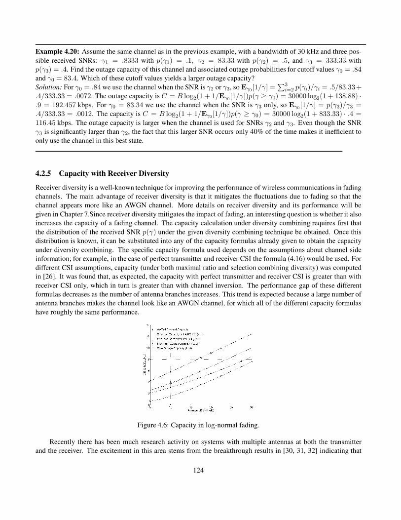
Example 4.20: Assume the same channel as in the previous example, with a bandwidth of 30 kHz and three pos-

sible received SNRs: γ1 = .8333 with p(γ1) = .1, γ2 = 83.33 with p(γ2) = .5, and γ3 = 333.33 with

p(γ3) = .4. Find the outage capacity of this channel and associated outage probabilities for cutoff values γ0 = .84and γ0 = 83.4. Which of these cutoff values yields a larger outage capacity?

Solution: For γ0 = .84 we use the channel when the SNR is γ2 or γ3, so Eγ0[1/γ] =∑3

i=2 p(γi)/γi = .5/83.33+.4/333.33 = .0072. The outage capacity is C = B log2(1 + 1/Eγ0[1/γ])p(γ ≥ γ0) = 30000 log2(1 + 138.88) ·.9 = 192.457 kbps. For γ0 = 83.34 we use the channel when the SNR is γ3 only, so Eγ0 [1/γ] = p(γ3)/γ3 =.4/333.33 = .0012. The capacity is C = B log2(1 + 1/Eγ0[1/γ])p(γ ≥ γ0) = 30000 log2(1 + 833.33) · .4 =

116.45 kbps. The outage capacity is larger when the channel is used for SNRs γ2 and γ3. Even though the SNR

γ3 is significantly larger than γ2, the fact that this larger SNR occurs only 40% of the time makes it inefficient to

only use the channel in this best state.

4.2.5 Capacity with Receiver Diversity

Receiver diversity is a well-known technique for improving the performance of wireless communications in fading

channels. The main advantage of receiver diversity is that it mitigates the fluctuations due to fading so that the

channel appears more like an AWGN channel. More details on receiver diversity and its performance will be

given in Chapter 7.Since receiver diversity mitigates the impact of fading, an interesting question is whether it also

increases the capacity of a fading channel. The capacity calculation under diversity combining requires first that

the distribution of the received SNR p(γ) under the given diversity combining technique be obtained. Once this

distribution is known, it can be substituted into any of the capacity formulas already given to obtain the capacity

under diversity combining. The specific capacity formula used depends on the assumptions about channel side

information; for example, in the case of perfect transmitter and receiver CSI the formula (4.16) would be used. For

different CSI assumptions, capacity (under both maximal ratio and selection combining diversity) was computed

in [26]. It was found that, as expected, the capacity with perfect transmitter and receiver CSI is greater than with

receiver CSI only, which in turn is greater than with channel inversion. The performance gap of these different

formulas decreases as the number of antenna branches increases. This trend is expected because a large number of

antenna branches makes the channel look like an AWGN channel, for which all of the different capacity formulas

have roughly the same performance.

Figure 4.6: Capacity in log-normal fading.

Recently there has been much research activity on systems with multiple antennas at both the transmitter

and the receiver. The excitement in this area stems from the breakthrough results in [30, 31, 32] indicating that

124

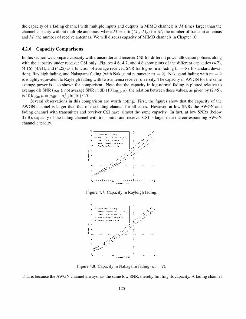
the capacity of a fading channel with multiple inputs and outputs (a MIMO channel) is M times larger than the

channel capacity without multiple antennas, where M = min(Mt, Mr) for Mt the number of transmit antennas

and Mr the number of receive antennas. We will discuss capacity of MIMO channels in Chapter 10.

4.2.6 Capacity Comparisons

In this section we compare capacity with transmitter and receiver CSI for different power allocation policies along

with the capacity under receiver CSI only. Figures 4.6, 4.7, and 4.8 show plots of the different capacities (4.7),

(4.16), (4.21), and (4.25) as a function of average received SNR for log-normal fading (σ = 8 dB standard devia-

tion), Rayleigh fading, and Nakagami fading (with Nakagami parameter m = 2). Nakagami fading with m = 2

is roughly equivalent to Rayleigh fading with two-antenna receiver diversity. The capacity in AWGN for the same

average power is also shown for comparison. Note that the capacity in log-normal fading is plotted relative to

average dB SNR (µdB), not average SNR in dB (10 log10 µ): the relation between these values, as given by (2.45),

is 10 log10 µ = µdB + σ2dB ln(10)/20.

Several observations in this comparison are worth noting. First, the figures show that the capacity of the

AWGN channel is larger than that of the fading channel for all cases. However, at low SNRs the AWGN and

fading channel with transmitter and receiver CSI have almost the same capacity. In fact, at low SNRs (below

0 dB), capacity of the fading channel with transmitter and receiver CSI is larger than the corresponding AWGN

channel capacity.

Figure 4.7: Capacity in Rayleigh fading.

Figure 4.8: Capacity in Nakagami fading (m = 2).

That is because the AWGN channel always has the same low SNR, thereby limiting its capacity. A fading channel

125

with this same low average SNR will occasionally have a high SNR, since the distribution has infinite range. Thus,

if high power and rate are transmitted over the channel during these very infrequent large SNR values, the capacity

will be greater than on the AWGN channel with the same low average SNR.

The severity of the fading is indicated by the Nakagami parameter m, where m = 1 for Rayleigh fading and

m = ∞ for an AWGN channel without fading. Thus, comparing Figures 4.7 and 4.8 we see that, as the severity

of the fading decreases (Rayleigh to Nakagami with m = 2), the capacity difference between the various adaptive

policies also decreases, and their respective capacities approach that of the AWGN channel.

The difference between the capacity curves under transmitter and receiver CSI (4.16) and receiver CSI only

(4.7) are negligible in all cases. Recalling that capacity under receiver CSI only (4.7) and under transmitter and

receiver CSI without power adaptation (4.10) are the same, we conclude that, if the transmission rate is adapted

relative to the channel, then adapting the power as well yields a negligible capacity gain. It also indicates that

transmitter adaptation yields a negligible capacity gain relative to using only receiver side information. In severe

fading conditions (Rayleigh and log-normal fading), maximum outage capacity exhibits a 1–5-dB rate penalty

and zero-outage capacity yields a large capacity loss relative to Shannon capacity. However, under mild fading

conditions (Nakagami with m = 2) the Shannon, maximum outage, and zero-outage capacities are within 3 dB of

each other and within 4 dB of the AWGN channel capacity. These differences will further decrease as the fading

diminishes (m → ∞ for Nakagami fading).

We can view these results as a trade-off between capacity and complexity. The adaptive policy with transmitter

and receiver side information requires more complexity in the transmitter (and typically also requires a feedback

path between the receiver and transmitter to obtain the side information). However, the decoder in the receiver is

relatively simple. The nonadaptive policy has a relatively simple transmission scheme, but its code design must

use the channel correlation statistics (often unknown) and the decoder complexity is proportional to the channel

decorrelation time. The channel inversion and truncated inversion policies use codes designed for AWGN channels

and thus are the least complex to implement, but in severe fading conditions they exhibit large capacity losses

relative to the other techniques.

In general, Shannon capacity analysis does not show how to design adaptive or non-adaptive techniques for

real systems. Achievable rates for adaptive trellis-coded MQAM have been investigated in [28], where a simple

four-state trellis code combined with adaptive six-constellation MQAM modulation was shown to achieve rates

within 7 dB of the Shannon capacity (4.12) in Figures 4.6 and 4.7. More complex codes further close the gap to

the Shannon limit of fading channels with transmitter adaptation.

4.3 Capacity of Frequency-Selective Fading Channels

In this section we examine the Shannon capacity of frequency-selective fading channels. We first consider the

capacity of a time-invariant frequency-selective fading channel. This capacity analysis is like that of a flat fading

channel but with the time axis replaced by the frequency axis. Then we discuss the capacity of time-varying

frequency-selective fading channels.

4.3.1 Time-Invariant Channels

Consider a time-invariant channel with frequency responseH(f), as shown in Figure 4.9. Assume a total transmit

power constraint P . When the channel is time invariant it is typically assumed that H(f) is known to both

the transmitter and receiver. The capacity of time-invariant channels under different assumptions about channel

knowledge are discussed in [23, 25].

Let us first assume that H(f) is block fading, so that frequency is divided into subchannels of bandwidth Bwith H(f) = Hj constant over each subchannel, as shown in Figure 4.10.

126

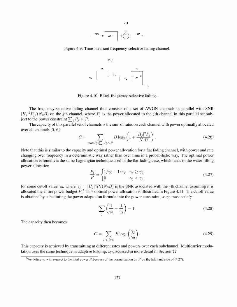
Figure 4.9: Time-invariant frequency-selective fading channel.

Figure 4.10: Block frequency-selective fading.

The frequency-selective fading channel thus consists of a set of AWGN channels in parallel with SNR

|Hj|2Pj/(N0B) on the jth channel, where Pj is the power allocated to the jth channel in this parallel set sub-

ject to the power constraint∑

j Pj ≤ P .

The capacity of this parallel set of channels is the sum of rates on each channel with power optimally allocated

over all channels [5, 6]:

C =∑

maxPj :P

j Pj≤P

B log2

(

1 +|Hj|2PjN0B

)

. (4.26)

Note that this is similar to the capacity and optimal power allocation for a flat fading channel, with power and rate

changing over frequency in a deterministic way rather than over time in a probabilistic way. The optimal power

allocation is found via the same Lagrangian technique used in the flat-fading case, which leads to the water-filling

power allocation

PjP

=

{

1/γ0 − 1/γj γj ≥ γ0,

0 γj < γ0,(4.27)

for some cutoff value γ0, where γj = |Hj|2P/(N0B) is the SNR associated with the jth channel assuming it is

allocated the entire power budget P .3 This optimal power allocation is illustrated in Figure 4.11. The cutoff value

is obtained by substituting the power adaptation formula into the power constraint, so γ0 must satisfy

∑

j

(

1

γ0− 1

γj

)

= 1. (4.28)

The capacity then becomes

C =∑

j:γj≥γ0

B log2

(

γjγ0

)

. (4.29)

This capacity is achieved by transmitting at different rates and powers over each subchannel. Multicarrier modu-

lation uses the same technique in adaptive loading, as discussed in more detail in Section ??.

3We define γj with respect to the total power P because of the normalization by P on the left hand side of (4.27).

127

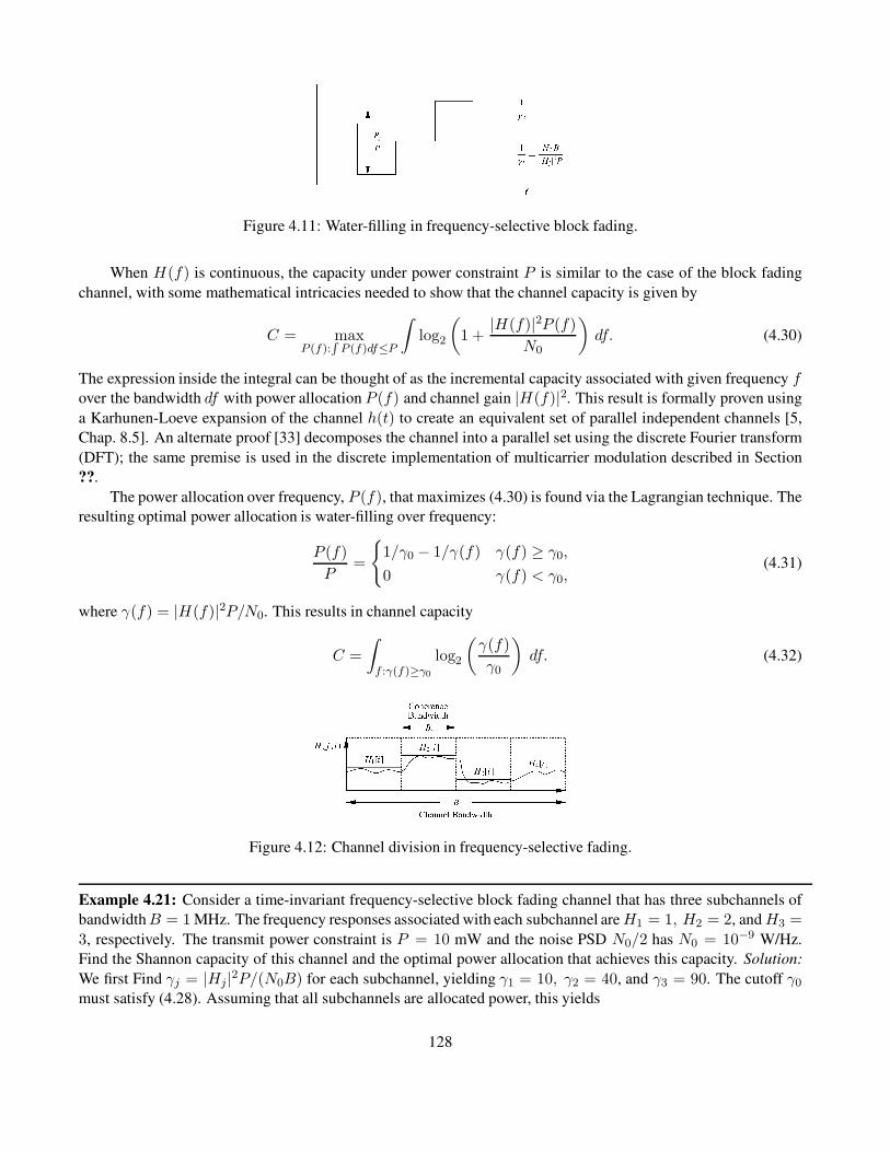
Figure 4.11: Water-filling in frequency-selective block fading.

When H(f) is continuous, the capacity under power constraint P is similar to the case of the block fading

channel, with some mathematical intricacies needed to show that the channel capacity is given by

C = maxP (f):

R

P (f)df≤P

∫

log2

(

1 +|H(f)|2P (f)

N0

)

df. (4.30)

The expression inside the integral can be thought of as the incremental capacity associated with given frequency fover the bandwidth df with power allocation P (f) and channel gain |H(f)|2. This result is formally proven using

a Karhunen-Loeve expansion of the channel h(t) to create an equivalent set of parallel independent channels [5,

Chap. 8.5]. An alternate proof [33] decomposes the channel into a parallel set using the discrete Fourier transform

(DFT); the same premise is used in the discrete implementation of multicarrier modulation described in Section

??.

The power allocation over frequency, P (f), that maximizes (4.30) is found via the Lagrangian technique. The

resulting optimal power allocation is water-filling over frequency:

P (f)

P=

{

1/γ0 − 1/γ(f) γ(f) ≥ γ0,

0 γ(f) < γ0,(4.31)

where γ(f) = |H(f)|2P/N0. This results in channel capacity

C =

∫

f :γ(f)≥γ0

log2

(

γ(f)

γ0

)

df. (4.32)

Figure 4.12: Channel division in frequency-selective fading.

Example 4.21: Consider a time-invariant frequency-selective block fading channel that has three subchannels of

bandwidthB = 1 MHz. The frequency responses associated with each subchannel areH1 = 1, H2 = 2, andH3 =

3, respectively. The transmit power constraint is P = 10 mW and the noise PSD N0/2 has N0 = 10−9 W/Hz.

Find the Shannon capacity of this channel and the optimal power allocation that achieves this capacity. Solution:

We first Find γj = |Hj|2P/(N0B) for each subchannel, yielding γ1 = 10, γ2 = 40, and γ3 = 90. The cutoff γ0

must satisfy (4.28). Assuming that all subchannels are allocated power, this yields

128

3

γ0= 1 +

∑

j

1

γj= 1.14 ⇒ γ0 = 2.64 < γj∀j.

Since the cutoff γ0 is less than γj for all j, our assumption that all subchannels are allocated power is consistent, so

this is the correct cutoff value. The corresponding capacity isC =∑3

j=1B log2(γj/γ0) = 1000000(log2(10/2.64)+

log2(40/2.64) + log2(90/2.64)) = 10.93 Mbps.

4.3.2 Time-Varying Channels

The time-varying frequency-selective fading channel is similar to the model shown in Figure 4.9 except that

H(f) = H(f, i); that is, the channel varies over both frequency and time. It is difficult to determine the capac-

ity of time-varying frequency-selective fading channels – even when the instantaneous channel H(f, i) is known

perfectly at the transmitter and receiver – because of the effects of self-interference (ISI). In the case of transmitter

and receiver side information, the optimal adaptation scheme must consider (a) the effect of the channel on the past

sequence of transmitted bits and (b) how the ISI resulting from these bits will affect future transmissions [34]. The

capacity of time-varying frequency-selective fading channels is in general unknown, but there do exist upper and

lower bounds as well as limiting formulas [34, 35].

We can approximate channel capacity in time-varying frequency-selective fading by taking the channel band-

width B of interest and then dividing it up into subchannels the size of the channel coherence bandwidth Bc, as

shown in Figure 4.12. We then assume that each of the resulting subchannels is independent, time varying, and flat

fading with H(f, i) = Hj[i] on the jth subchannel.

Under this assumption, we obtain the capacity for each of these flat fading subchannels based on the average

power Pj that we allocate to each subchannel, subject to a total power constraint P . Since the channels are

independent, the total channel capacity is just equal to the sum of capacities on the individual narrowband flat

fading channels – subject to the total average power constraint and averaged over both time and frequency:

C = max{Pj}:

P

j Pj≤P

∑

j

Cj(Pj), (4.33)

where Cj(Pj) is the capacity of the flat fading subchannel with average power Pj and bandwidth Bc given by

(4.16), (4.7), (4.21), or (4.25) for Shannon capacity under different side information and power allocation policies.

We can also define Cj(Pj) as a capacity versus outage if only the receiver has side information.

We will focus on Shannon capacity assuming perfect transmitter and receiver channel CSI, since this up-

perbounds capacity under any other side information assumptions or suboptimal power allocation strategies. We

know that if we fix the average power per subchannel then the optimal power adaptation follows a water-filling for-

mula. We expect that the optimal average power to be allocated to each subchannel will also follow a water-filling

formula, where more average power is allocated to better subchannels. Thus we expect that the optimal power allo-

cation is a two-dimensional water-filling in both time and frequency. We now obtain this optimal two-dimensional

water-filling and the corresponding Shannon capacity.

Define γj[i] = |Hj[i]|2P /(N0B) to be the instantaneous SNR on the jth subchannel at time i assuming the

total power P is allocated to that time and frequency. We allow the power Pj(γj) to vary with γj[i]. The Shannon

capacity with perfect transmitter and receiver CSI is given by optimizing power adaptation relative to both time

(represented by γj[i] = γj) and frequency (represented by the subchannel index j):

C = maxPj(γj ):

P

j

R

∞

0Pj (γj)p(γj)dγj≤P

∑

j

∫ ∞

0

Bc log2

(

1 +Pj(γj)γj

P

)

p(γj)dγj. (4.34)

129

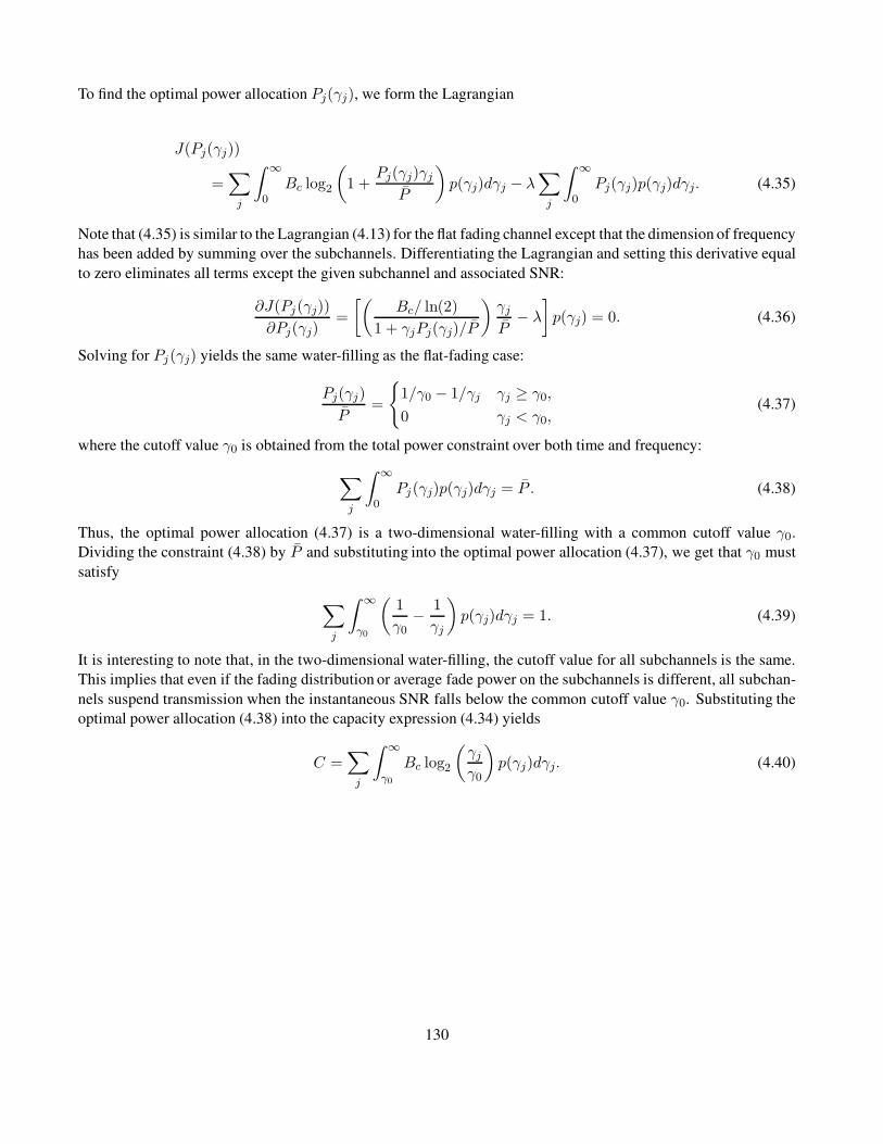
To find the optimal power allocation Pj(γj), we form the Lagrangian

J(Pj(γj))

=∑

j

∫ ∞

0Bc log2

(

1 +Pj(γj)γj

P

)

p(γj)dγj − λ∑

j

∫ ∞

0Pj(γj)p(γj)dγj. (4.35)

Note that (4.35) is similar to the Lagrangian (4.13) for the flat fading channel except that the dimension of frequency

has been added by summing over the subchannels. Differentiating the Lagrangian and setting this derivative equal

to zero eliminates all terms except the given subchannel and associated SNR:

∂J(Pj(γj))

∂Pj(γj)=

[(

Bc/ ln(2)

1 + γjPj(γj)/P

)

γj

P− λ

]

p(γj) = 0. (4.36)

Solving for Pj(γj) yields the same water-filling as the flat-fading case:

Pj(γj)

P=

{

1/γ0 − 1/γj γj ≥ γ0,

0 γj < γ0,(4.37)

where the cutoff value γ0 is obtained from the total power constraint over both time and frequency:

∑

j

∫ ∞

0Pj(γj)p(γj)dγj = P . (4.38)

Thus, the optimal power allocation (4.37) is a two-dimensional water-filling with a common cutoff value γ0.

Dividing the constraint (4.38) by P and substituting into the optimal power allocation (4.37), we get that γ0 must

satisfy

∑

j

∫ ∞

γ0

(

1

γ0− 1

γj

)

p(γj)dγj = 1. (4.39)

It is interesting to note that, in the two-dimensional water-filling, the cutoff value for all subchannels is the same.

This implies that even if the fading distribution or average fade power on the subchannels is different, all subchan-

nels suspend transmission when the instantaneous SNR falls below the common cutoff value γ0. Substituting the

optimal power allocation (4.38) into the capacity expression (4.34) yields

C =∑

j

∫ ∞

γ0

Bc log2

(

γjγ0

)

p(γj)dγj. (4.40)

130

Chapter 4 Problems

1. Capacity in AWGN is given by C = B log2(1 + P/(N0B)), where P is the received signal power, B is the

signal bandwidth, and N0/2 is the noise PSD. Find capacity in the limit of infinite bandwidth B → ∞ as a

function of P .

2. Consider an AWGN channel with bandwidth 50 MHz, received signal power 10 mW, and noise PSD N0/2whereN0 = 2 · 10−9 W/Hz. How much does capacity increase by doubling the received power? How much

does capacity increase by doubling the channel bandwidth?

3. Consider two users simultaneously transmitting to a single receiver in an AWGN channel. This is a typical

scenario in a cellular system with multiple users sending signals to a base station. Assume the users have

equal received power of 10 mW and total noise at the receiver in the bandwidth of interest of 0.1 mW. The

channel bandwidth for each user is 20 MHz.

(a) Suppose that the receiver decodes user 1’s signal first. In this decoding, user 2’s signal acts as noise (as-

sume it has the same statistics as AWGN). What is the capacity of user 1’s channel with this additional

interference noise?

(b) Suppose that, after decoding user 1’s signal, the decoder re-encodes it and subtracts it out of the re-

ceived signal. Now, in the decoding of user 2’s signal, there is no interference from user 1’s signal.

What then is the Shannon capacity of user 2’s channel?

Note: We will see in Chapter 14 that the decoding strategy of successively subtracting out decoded signals

is optimal for achieving Shannon capacity of a multiuser channel with independent transmitters sending to

one receiver.

4. Consider a flat fading channel of bandwidth 20 MHz and where, for a fixed transmit power P , the received

SNR is one of six values: γ1 = 20 dB, γ2 = 15 dB, γ3 = 10 dB, γ4 = 5 dB, γ5 = 0 dB, and γ6 = −5 dB.

The probabilities associated with each state are p1 = p6 = .1, p2 = p4 = .15, and p3 = p5 = .25. Assume

that only the receiver has CSI.

(a) Find the Shannon capacity of this channel.

(b) Plot the capacity versus outage for 0 ≤ Pout < 1 and find the maximum average rate that can be

correctly received (maximum Cout).

5. Consider a flat fading channel in which, for a fixed transmit power P , the received SNR is one of four values:

γ1 = 30 dB, γ2 = 20 dB, γ3 = 10 dB, and γ4 = 0 dB. The probabilities associated with each state are

p1 = .2, p2 = .3, p3 = .3, and p4 = .2. Assume that both transmitter and receiver have CSI.

(a) Find the optimal power adaptation policy P [i]/P for this channel and its corresponding Shannon ca-

pacity per unit hertz (C/B).

(b) Find the channel inversion power adaptation policy for this channel and associated zero-outage capacity

per unit bandwidth.

(c) Find the truncated channel inversion power adaptation policy for this channel and associated outage

capacity per unit bandwidth for three different outage probabilities: Pout = .1, Pout = .25, and Pout

(and the associated cutoff γ0) equal to the value that achieves maximum outage capacity.

131

6. Consider a cellular system where the power falloff with distance follows the formula Pr(d) = Pt(d0/d)α,

where d0 = 100 m and α is a random variable. The distribution for α is p(α = 2) = .4, p(α = 2.5) =

.3, p(α = 3) = .2, and p(α = 4) = .1. Assume a receiver at a distance d = 1000 m from the transmitter,

with an average transmit power constraint of Pt = 100 mW and a receiver noise power of .1 mW. Assume

that both transmitter and receiver have CSI.

(a) Compute the distribution of the received SNR.

(b) Derive the optimal power adaptation policy for this channel and its corresponding Shannon capacity

per unit hertz (C/B).

(c) Determine the zero-outage capacity per unit bandwidth of this channel.

(d) Determine the maximum outage capacity per unit bandwidth of this channel.

7. In this problem we explore power allocation under a fixed energy constraint to maximize the number of bits

transmitted. Consider a cellular system with a mobile receiver. The receiver stops at point A (100m from

the cell phone tower) for 10 minutes and point B (500m from the cell phone tower) for 20 minutes. Assume

the signal from the cell phone tower to the receiver only experiences path loss under the simplified path loss

model with γ = 3, d0 = 1m, and K = 1 along with AWGN, that the channel bandwidth is 20MHz, and the

receiver noise PSD is N0 = 5 × 10−14mW/Hz. Also, assume a fixed transmit power of 1mW.

(a) What is the SNR received at points A and B?

(b) What is total amount of energy (in Joules) that is transmitted during the two stops.

(c) Assuming the transmitter sends data with a rate equal to the Shannon capacity of the channel at each

of the stops, what is the total number of bits received?

(d) Suppose now that the cell phone tower does not send at a fixed transmit power but fixes the total

number of Joules it will transmit to the receiver at each of the two stops. Using the total amount of

energy derived in part (b), determine the optimal allocation of this total energy at each of the stops to

maximize the number of bits received. Assume that the transmitter sends data at a rate equal to the

Shannon capacity with SNR based on your optimal energy allocation. How many bits are received

with this optimal energy allocation and how does it compare to your answer in part (c)?

8. In this problem we explore why channel inversion leads to zero capacity in Rayleigh fading. Assume a

Rayleigh fading channel with γ = 1 so the receiver power has an exponential distribution p(γ) = e−γ .

(a) Show using a first-order Taylor series expansion of e−γ around γ = 0 that p(γ) = e−γ > 1 − γ .

(b) We will now show that E[

1γ

]

is unbounded by taking the expectation for γ ∈ (0, c) for some small

constant c. Fix this small constant c and a smaller constant ε < c. Then compute the following lower

bound for E[

1γ

]

by taking the expectation over the interval (ε, c) and using the lower bound on p(γ)

from part (a):

E

[

1

γ

]

>

∫ c

ε

1

γ(1 − γ)dγ.

Show that as ε → 0, the above expression becomes unbounded. This suggests that the transmit power

needed to maintain a constant received power by inverting Rayleigh fading is unbounded.

9. Assume a Rayleigh fading channel, where the transmitter and receiver have CSI and the distribution of the

fading SNR p(γ) is exponential with mean γ = 10 dB. Assume a channel bandwidth of 10 MHz.

132

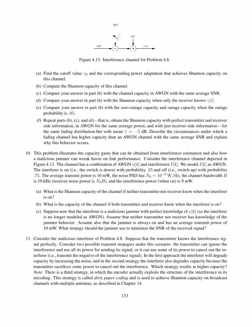
Figure 4.13: Interference channel for Problem 4.8.

(a) Find the cutoff value γ0 and the corresponding power adaptation that achieves Shannon capacity on

this channel.

(b) Compute the Shannon capacity of this channel.

(c) Compare your answer in part (b) with the channel capacity in AWGN with the same average SNR.

(d) Compare your answer in part (b) with the Shannon capacity when only the receiver knows γ[i].

(e) Compare your answer in part (b) with the zero-outage capacity and outage capacity when the outage

probability is .05.

(f) Repeat parts (b), (c), and (d) – that is, obtain the Shannon capacity with perfect transmitter and receiver

side information, in AWGN for the same average power, and with just receiver side information – for

the same fading distribution but with mean γ = −5 dB. Describe the circumstances under which a

fading channel has higher capacity than an AWGN channel with the same average SNR and explain

why this behavior occurs.

10. This problem illustrates the capacity gains that can be obtained from interference estimation and also how

a malicious jammer can wreak havoc on link performance. Consider the interference channel depicted in

Figure 4.13. The channel has a combination of AWGN n[k] and interference I [k]. We model I [k] as AWGN.

The interferer is on (i.e., the switch is down) with probability .25 and off (i.e., switch up) with probability

.75. The average transmit power is 10 mW, the noise PSD has N0 = 10−8 W/Hz, the channel bandwidthBis 10 kHz (receiver noise power is N0B), and the interference power (when on) is 9 mW.

(a) What is the Shannon capacity of the channel if neither transmitter nor receiver know when the interferer

is on?

(b) What is the capacity of the channel if both transmitter and receiver know when the interferer is on?

(c) Suppose now that the interferer is a malicious jammer with perfect knowledge of x[k] (so the interferer

is no longer modeled as AWGN). Assume that neither transmitter nor receiver has knowledge of the

jammer behavior. Assume also that the jammer is always on and has an average transmit power of

10 mW. What strategy should the jammer use to minimize the SNR of the received signal?

11. Consider the malicious interferer of Problem 4.8. Suppose that the transmitter knows the interference sig-

nal perfectly. Consider two possible transmit strategies under this scenario: the transmitter can ignore the

interference and use all its power for sending its signal, or it can use some of its power to cancel out the in-

terferer (i.e., transmit the negative of the interference signal). In the first approach the interferer will degrade

capacity by increasing the noise, and in the second strategy the interferer also degrades capacity because the

transmitter sacrifices some power to cancel out the interference. Which strategy results in higher capacity?

Note: There is a third strategy, in which the encoder actually exploits the structure of the interference in its

encoding. This strategy is called dirty paper coding and is used to achieve Shannon capacity on broadcast

channels with multiple antennas, as described in Chapter 14.

133

12. Show using Lagrangian techniques that the optimal power allocation to maximize the capacity of a time-

invariant block fading channel is given by the water-filling formula in (4.27).

13. Consider a time-invariant block fading channel with frequency response

H(f) =

1 fc − 20 MHz ≤ f < fc − 10 MHz,

.5 fc − 10 MHz ≤ f < fc,

2 fc ≤ f < fc + 10 MHz,

.25 fc + 10 MHz ≤ f < fc + 20 MHz,

0 else,

for f > 0 and H(−f) = H(f). For a transmit power of 10 mW and a noise PSD of .001 µW per Hertz,

find the optimal power allocation and corresponding Shannon capacity of this channel.

14. Show that the optimal power allocation to maximize the capacity of a time-invariant frequency-selective

fading channel is given by the water-filling formula in (4.31).

15. Consider a frequency-selective fading channel with total bandwidth 12 MHz and coherence bandwidthBc =4 MHz. Divide the total bandwidth into three subchannels of bandwidthBc, and assume that each subchannel

is a Rayleigh flat fading channel with independent fading on each subchannel. Assume the subchannels have

average gains E[|H1[i]|2] = 1, E[|H2[i]|2] = .5, and E[|H3[i]|2] = .125. Assume a total transmit power of

30 mW and a receiver noise PSD with N0 = .001 µW/Hz.

(a) Find the optimal two-dimensional water-filling power adaptation for this channel and the corresponding

Shannon capacity, assuming both transmitter and receiver know the instantaneous value of Hj[i], j =1, 2, 3.

(b) Compare the capacity derived in part (a) with that obtained by allocating an equal average power of

10 mW to each subchannel and then water-filling on each subchannel relative to this power allocation.

134

Bibliography

[1] C. E. Shannon, “A mathematical theory of communication,” Bell System Tech. J ., pp. 379–423, 623–56,

1948.

[2] C. E. Shannon, “Communications in the presence of noise.” Proc. IRE, pp. 10–21, 1949.

[3] C. E. Shannon and W. Weaver, The Mathematical Theory of Communication, University of Illinois Press,

Urbana, 1949.

[4] M. Medard, “The effect upon channel capacity in wireless communications of perfect and imperfect knowl-

edge of the channel,” IEEE Trans. Inform. Theory, pp. 933–46, May 2000.

[5] R. G. Gallager, Information Theory and Reliable Communication, Wiley, New York, 1968.

[6] T. Cover and J. Thomas, Elements of Information Theory, Wiley, New York, 2nd Ed, 2006.

[7] Y. Polyanskiy, H. V. Poor and S. Verdu, “Channel Coding Rate in the Finite Blocklength Regime,” IEEE

Transactions on Information Theory, vol. 56, no. 5, pp. 2307-2359, May 2010.

[8] C. Berrou, A. Glavieux, “Near optimum error correcting coding and decoding: Turbo-codes”, IEEE Trans-

actions on Commununications, vol. 44, no. 10, pp. 1261-1271, Oct. 1996.

[9] R.G. Gallager, Low-Density Parity-Check Codes. Cambridge, MA: MIT Press, 1963 (Sc.D. MIT, 1960).

[10] R. Urbanke, B. Rimoldi, “Lattice codes can achieve capacity on the AWGN channel”, IEEE Transactions on

Information Theory, vol. 44, no. 1, pp. 273-278, Jan. 1998.

[11] E. Arikan, “Channel polarization: A method for constructing capacity-achieving codes for symmetric binary-

input memoryless channels”, IEEE Transactions on Information Theory, vol. 55, no. 7, pp. 3051-3073, July

2009.

[12] I. Csiszar and J. Korner, Information Theory: Coding Theorems for Discrete Memoryless Channels, Aca-

demic Press, New York, 1981.

[13] I. Csiszar and P. Narayan, “The capacity of the arbitrarily varying channel,” IEEE Trans. Inform. Theory, pp.

18–26, January 1991.

[14] I. C. Abou-Faycal, M. D. Trott, and S. Shamai, “The capacity of discrete-time memoryless Rayleigh fading

channels,” IEEE Trans. Inform. Theory, pp. 1290–1301, May 2001.

[15] A. Lapidoth and S. M. Moser, “Capacity bounds via duality with applications to multiple-antenna systems on

flat-fading channels,” IEEE Trans. Inform. Theory, pp. 2426–67, October 2003.

135

[16] A. J. Goldsmith and P. P. Varaiya, “Capacity, mutual information, and coding for finite-state Markov chan-

nels,” IEEE Trans. Inform. Theory, pp. 868–86, May 1996.

[17] M. Mushkin and I. Bar-David, “Capacity and coding for the Gilbert-Elliot channel,” IEEE Trans. Inform.

Theory, pp. 1277–90, November 1989.

[18] T. Holliday, A. Goldsmith, and P. Glynn, “Capacity of finite state Markov channels with general inputs,”

Proc. IEEE Internat. Sympos. Inform. Theory, p. 289, July 2003.

[19] R. J. McEliece and W. E. Stark, “Channels with block interference,” IEEE Trans. Inform. Theory, pp. 44–53,

January 1984.

[20] A. Lapidoth and S. Shamai, “Fading channels: How perfect need ‘perfect side information’ be?” IEEE Trans.

Inform. Theory, pp. 1118–34, November 1997.

[21] G. J. Foschini, D. Chizhik, M. Gans, C. Papadias, and R. A. Valenzuela, “Analysis and performance of some

basic space-time architectures,” IEEE J. Sel. Areas Commun., pp. 303–20, April 2003.

[22] W. L. Root and P. P. Varaiya, “Capacity of classes of Gaussian channels,” SIAM J. Appl. Math., pp. 1350–93,

November 1968.

[23] J. Wolfowitz, Coding Theorems of Information Theory, 2nd ed., Springer-Verlag, New York, 1964.

[24] A. J. Goldsmith and P. P. Varaiya, “Capacity of fading channels with channel side information,” IEEE Trans.

Inform. Theory, pp. 1986–92, November 1997.

[25] G. Caire and S. Shamai, “On the capacity of some channels with channel state information,” IEEE Trans.

Inform. Theory, pp. 2007–19, September 1999.

[26] M.-S. Alouini and A. J. Goldsmith, “Capacity of Rayleigh fading channels under different adaptive transmis-

sion and diversity combining techniques,” IEEE Trans. Veh. Tech. pp. 1165–81, July 1999.

[27] S.-G. Chua and A. J. Goldsmith, “Variable-rate variable-power MQAM for fading channels,” IEEE Trans.

Commun., pp. 1218–30, October 1997.

[28] S.-G. Chua and A. J. Goldsmith, “Adaptive coded modulation for fading channels,” IEEE Trans. Commun.,

pp. 595–602, May 1998.

[29] K. S. Gilhousen, I. M. Jacobs, R. Padovani, A. J. Viterbi, L. A. Weaver, Jr., and C. E. Wheatley III, “On the

capacity of a cellular CDMA system,” IEEE Trans. Veh. Tech. pp. 303–12, May 1991.

[30] G. J. Foschini, “Layered space-time architecture for wireless communication in fading environments when

using multi-element antennas,” Bell System Tech. J ., pp. 41–59, Autumn 1996.

[31] E. Teletar, “Capacity of multi-antenna Gaussian channels,” AT&T Bell Labs Intemal Tech. Memo, June 1995.

[32] G. J. Foschini and M. Gans, “On limits of wireless communications in a fading environment when using

multiple antennas,” Wireless Pers. Commun., pp. 311–35, March 1998.

[33] W. Hirt and J. L. Massey, “Capacity of the discrete-time Gaussian channel with intersymbol interference,”

IEEE Trans. Inform. Theory, pp. 380–8, May 1988.

136

[34] A. Goldsmith and M. Medard, “Capacity of time-varying channels with channel side information,” IEEE

Trans. Inform. Theory Vol. 53, No. 3, pp. 881-899, March 2007.

[35] S. Diggavi, ‘Analysis of multicarrier transmission in time-varying channels,” Proc. IEEE Internat. Conf.

Commun., pp. 1191–5, June 1997.

137

Chapter 5

Digital Modulation and Detection

The advances over the last several decades in hardware and digital signal processing have made digital transceivers

much cheaper, faster, and more power efficient than analog transceivers. More importantly, digital modulation

offers a number of other advantages over analog modulation, including higher spectral efficiency, powerful error

correction techniques, resistance to channel impairments, more efficient multiple access strategies, and better secu-

rity and privacy. Specifically, high-level digital modulation techniques such as MQAM allow much more efficient

use of spectrum than is possible with analog modulation. Advances in coding and coded modulation applied to dig-

ital signaling make the signal much less susceptible to noise and fading, and equalization or multicarrier techniques

can be used to mitigate intersymbol interference (ISI). Spread-spectrum techniques applied to digital modulation

can simultaneously remove or combine multipath, resist interference, and detect multiple users. Finally, digital

modulation is much easier to encrypt, resulting in a higher level of security and privacy for digital systems. For all

these reasons, systems currently being built or proposed for wireless applications are all digital systems.

Digital modulation and detection consist of transferring information in the form of bits over a communication

channel. The bits are binary digits taking on the values of either 1 or 0. These information bits are derived

from the information source, which may be a digital source or an analog source that has been passed through

an A/D converter. Both digital and A/D-converted analog sources may be compressed to obtain the information

bit sequence. Digital modulation consists of mapping the information bits into an analog signal for transmission

over the channel. Detection consists of estimating the original bit sequence based on the signal received over the

channel. The main considerations in choosing a particular digital modulation technique are high data rate; high

spectral efficiency (minimum bandwidth occupancy); high power efficiency (minimum required transmit power);

robustness to channel impairments (minimum probability of bit error); and low power/cost implementation. Often

these are conflicting requirements, and the choice of modulation is based on finding the technique that achieves the

best trade-off between them.

There are two main categories of digital modulation: amplitude/phase modulation and frequency modulation.

Since frequency modulation typically has a constant signal envelope and is generated using nonlinear techniques,

this modulation is also called constant envelope modulation or nonlinear modulation, and amplitude/phase mod-

ulation is also called linear modulation. Linear modulation generally has better spectral properties than nonlinear

modulation, since nonlinear processing leads to spectral broadening. However, amplitude and phase modulation

embeds the information bits into the amplitude or phase of the transmitted signal, which is more susceptible to

variations from fading and interference. In addition, amplitude and phase modulation techniques typically require

linear amplifiers, which are more expensive and less power efficient than the nonlinear amplifiers that can be used

with nonlinear modulation. Thus, the trade-off between linear versus nonlinear modulation is one of better spectral

efficiency for the former technique and better power efficiency and resistance to channel impairments for the lat-

ter. Once the modulation technique is determined, the constellation size must be chosen. Modulations with large

138

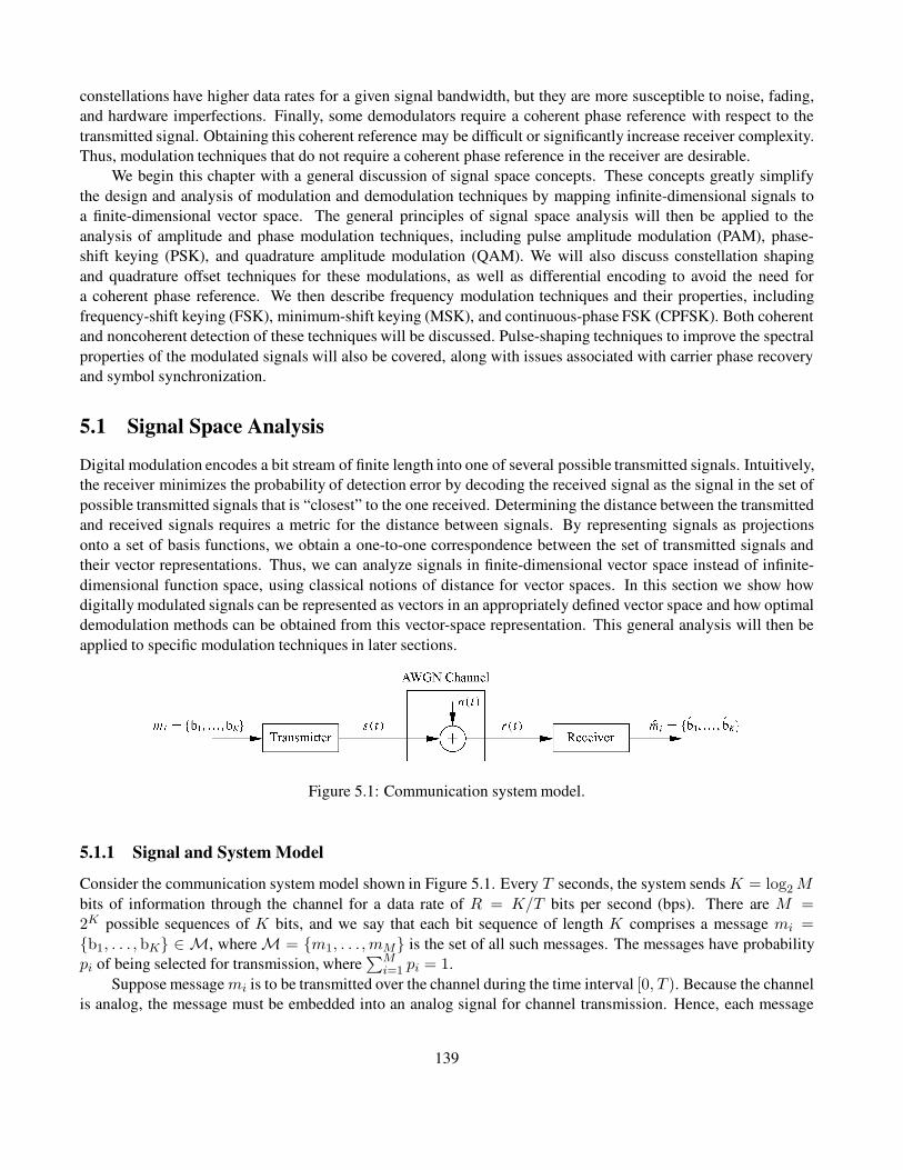
constellations have higher data rates for a given signal bandwidth, but they are more susceptible to noise, fading,

and hardware imperfections. Finally, some demodulators require a coherent phase reference with respect to the

transmitted signal. Obtaining this coherent reference may be difficult or significantly increase receiver complexity.

Thus, modulation techniques that do not require a coherent phase reference in the receiver are desirable.

We begin this chapter with a general discussion of signal space concepts. These concepts greatly simplify

the design and analysis of modulation and demodulation techniques by mapping infinite-dimensional signals to

a finite-dimensional vector space. The general principles of signal space analysis will then be applied to the

analysis of amplitude and phase modulation techniques, including pulse amplitude modulation (PAM), phase-

shift keying (PSK), and quadrature amplitude modulation (QAM). We will also discuss constellation shaping

and quadrature offset techniques for these modulations, as well as differential encoding to avoid the need for

a coherent phase reference. We then describe frequency modulation techniques and their properties, including

frequency-shift keying (FSK), minimum-shift keying (MSK), and continuous-phase FSK (CPFSK). Both coherent

and noncoherent detection of these techniques will be discussed. Pulse-shaping techniques to improve the spectral

properties of the modulated signals will also be covered, along with issues associated with carrier phase recovery

and symbol synchronization.

5.1 Signal Space Analysis

Digital modulation encodes a bit stream of finite length into one of several possible transmitted signals. Intuitively,

the receiver minimizes the probability of detection error by decoding the received signal as the signal in the set of

possible transmitted signals that is “closest” to the one received. Determining the distance between the transmitted

and received signals requires a metric for the distance between signals. By representing signals as projections

onto a set of basis functions, we obtain a one-to-one correspondence between the set of transmitted signals and

their vector representations. Thus, we can analyze signals in finite-dimensional vector space instead of infinite-

dimensional function space, using classical notions of distance for vector spaces. In this section we show how

digitally modulated signals can be represented as vectors in an appropriately defined vector space and how optimal

demodulation methods can be obtained from this vector-space representation. This general analysis will then be

applied to specific modulation techniques in later sections.

Figure 5.1: Communication system model.

5.1.1 Signal and System Model

Consider the communication system model shown in Figure 5.1. Every T seconds, the system sends K = log2M

bits of information through the channel for a data rate of R = K/T bits per second (bps). There are M =2K possible sequences of K bits, and we say that each bit sequence of length K comprises a message mi =

{b1, . . . , bK} ∈ M, where M = {m1, . . . , mM} is the set of all such messages. The messages have probability

pi of being selected for transmission, where∑M

i=1 pi = 1.

Suppose messagemi is to be transmitted over the channel during the time interval [0, T ). Because the channel

is analog, the message must be embedded into an analog signal for channel transmission. Hence, each message

139

mi ∈ M is mapped to a unique analog signal si(t) ∈ S = {s1(t), . . . , sM(t)}, where si(t) is defined on the time

interval [0, T ) and has energy

Esi =

∫ T

0s2i (t)dt, i = 1, . . . ,M. (5.1)

Since each message represents a bit sequence it follows that each signal si(t) ∈ S also represents a bit

sequence, and detection of the transmitted signal si(t) at the receiver is equivalent to detection of the transmitted

bit sequence. When messages are sent sequentially, the transmitted signal becomes a sequence of the corresponding

analog signals over each time interval [kT, (k+1)T ) : s(t) =∑

k si(t−kT ), where si(t) is a baseband or passband

analog signal corresponding to the message mi designated for the transmission interval [kT, (k + 1)T ). This is

illustrated in Figure 5.2, where we show the transmitted signal s(t) = s1(t)+s2(t−T )+s1(t−2T )+s1(t−3T )corresponding to the string of messages m1, m2, m1, m1 with message mi mapped to signal si(t).

In the model of Figure 5.1, the transmitted signal is sent through an AWGN channel, where a white Gaussian

noise process n(t) of power spectral density N0/2 is added to form the received signal r(t) = s(t) + n(t). Given

r(t), the receiver must determine the best estimate of which si(t) ∈ S was transmitted during each transmission

interval [kT, (k+ 1)T ). This best estimate for si(t) is mapped to a best estimate of the message mi(t) ∈ M and

the receiver then outputs this best estimate m = {b1, . . . , bK} ∈ M of the transmitted bit sequence.

The goal of the receiver design in estimating the transmitted message is to minimize the probability of message

error,

Pe =

M∑

i=1

p(m 6= mi|mi sent)p(mi sent), (5.2)

Figure 5.2: Transmitted signal for a sequence of messages.

over each time interval [kT, (k + 1)T ). By representing the signals {si(t) : i = 1, . . . ,M} geometrically, we

can solve for the optimal receiver design in AWGN based on a minimum distance criterion. Note that, as we saw

in previous chapters, wireless channels typically have a time-varying impulse response in addition to AWGN. We

will consider the effect of an arbitrary channel impulse response on digital modulation performance in Chapter

6;methods to combat this performance degradation are discussed in Chapters 11–13.

5.1.2 Geometric Representation of Signals

The basic premise behind a geometrical representation of signals is the notion of a basis set. Specifically, us-

ing a Gram–Schmidt orthogonalization procedure [1, 2], it can be shown that any set of M real signals S ={s1(t), . . . , sM(t)} defined on [0, T ) with finite energy can be represented as a linear combination of N ≤M real

orthonormal basis functions {φ1(t), . . . , φN(t)}. We say that these basis functions span the set S. Thus, we can

write each si(t) ∈ S in terms of its basis function representation as

140

si(t) =

N∑

j=1

sijφj(t), 0 ≤ t < T, (5.3)

where

sij =

∫ T

0si(t)φj(t)dt (5.4)

is a real coefficient representing the projection of si(t) onto the basis function φj(t) and

∫ T

0φi(t)φj(t)dt =

{

1 i = j,

0 i 6= j.(5.5)

If the signals {si(t)} are linearly independent then N = M , otherwiseN < M . Moreover, the minimum number

N of orthogonal basis functions needed to represent any signal si(t) of duration T and bandwidth B is roughly

2BT [3, Chap. 5.3]. The signal si(t) thus occupies 2BT orthogonal dimensions.

For linear passband modulation techniques, the basis set consists of the sine and cosine functions:

φ1(t) =

√

2

Tcos(2πfct) (5.6)

and

φ2(t) =

√

2

Tsin(2πfct). (5.7)

The√

2/T factor is needed for normalization so that∫ T0 φ2

i (t) dt = 1, i = 1, 2. In fact, with these basis functions

we get only an approximation to (5.5), since

∫ T

0φ2

1(t) dt =2

T

∫ T

0.5[1 + cos(4πfct)] dt = 1 +

sin(4πfcT )

4πfcT. (5.8)

The numerator in the second term of (5.8) is bounded by 1 and for fcT � 1 the denominator of this term is very

large. Hence this second term can be neglected. Similarly,

∫ T

0φ1(t)φ2(t) dt =

2

T

∫ T

0.5 sin(4πfct) dt =

− cos(4πfcT )

4πfcT≈ 0, (5.9)

where the approximation is taken as an equality for fcT � 1.

With the basis set φ1(t) =√

2/T cos(2πfct) and φ2(t) =√

2/T sin(2πfct), the basis function represen-

tation (5.3) corresponds to the equivalent lowpass representation of si(t) in terms of its in-phase and quadrature

components:

si(t) = si1

√

2

Tcos(2πfct) + si2

√

2

Tsin(2πfct). (5.10)

Note that the carrier basis functions may have an initial phase offset φ0. The basis set may also include a baseband

pulse-shaping filter g(t) to improve the spectral characteristics of the transmitted signal:

si(t) = si1g(t) cos(2πfct) + si2g(t) sin(2πfct). (5.11)

141

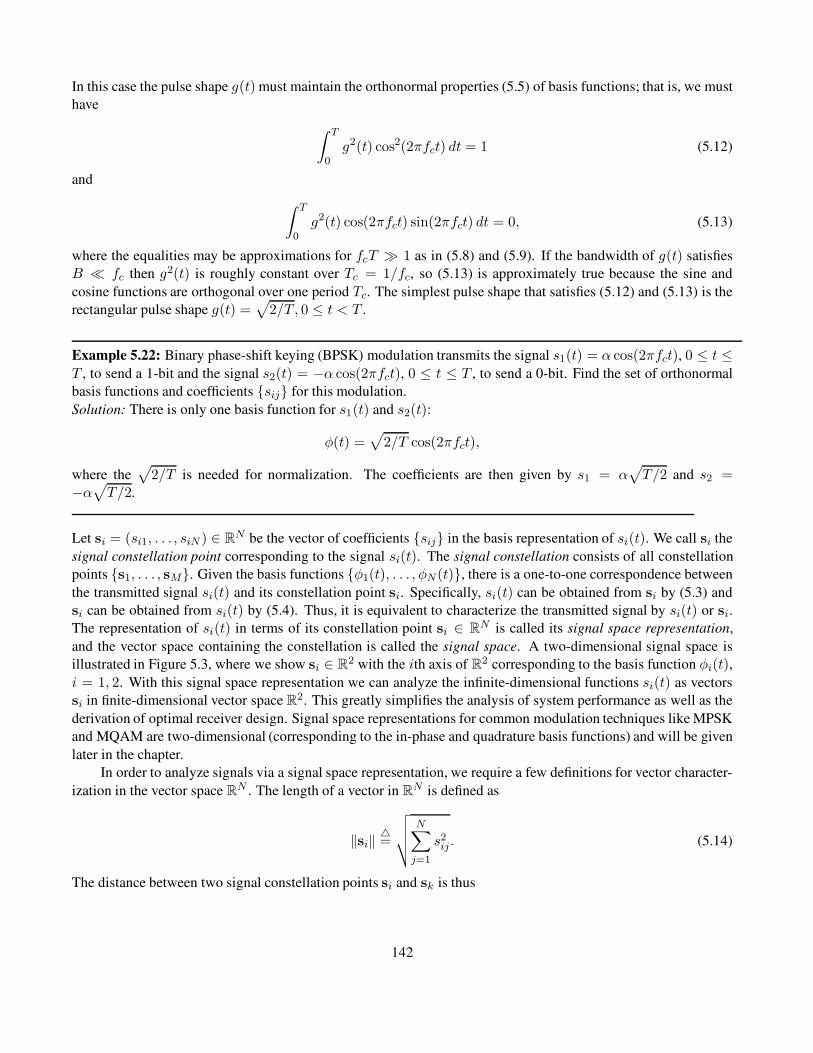
In this case the pulse shape g(t) must maintain the orthonormal properties (5.5) of basis functions; that is, we must

have

∫ T

0g2(t) cos2(2πfct) dt = 1 (5.12)

and

∫ T

0g2(t) cos(2πfct) sin(2πfct) dt = 0, (5.13)

where the equalities may be approximations for fcT � 1 as in (5.8) and (5.9). If the bandwidth of g(t) satisfies

B � fc then g2(t) is roughly constant over Tc = 1/fc, so (5.13) is approximately true because the sine and

cosine functions are orthogonal over one period Tc. The simplest pulse shape that satisfies (5.12) and (5.13) is the

rectangular pulse shape g(t) =√

2/T, 0 ≤ t < T .

Example 5.22: Binary phase-shift keying (BPSK) modulation transmits the signal s1(t) = α cos(2πfct), 0 ≤ t ≤T , to send a 1-bit and the signal s2(t) = −α cos(2πfct), 0 ≤ t ≤ T , to send a 0-bit. Find the set of orthonormal

basis functions and coefficients {sij} for this modulation.

Solution: There is only one basis function for s1(t) and s2(t):

φ(t) =√

2/T cos(2πfct),

where the√

2/T is needed for normalization. The coefficients are then given by s1 = α√

T/2 and s2 =−α√

T/2.

Let si = (si1, . . . , siN ) ∈ RN be the vector of coefficients {sij} in the basis representation of si(t). We call si the

signal constellation point corresponding to the signal si(t). The signal constellation consists of all constellation

points {s1, . . . , sM}. Given the basis functions {φ1(t), . . . , φN(t)}, there is a one-to-one correspondence between

the transmitted signal si(t) and its constellation point si. Specifically, si(t) can be obtained from si by (5.3) and

si can be obtained from si(t) by (5.4). Thus, it is equivalent to characterize the transmitted signal by si(t) or si.The representation of si(t) in terms of its constellation point si ∈ R

N is called its signal space representation,

and the vector space containing the constellation is called the signal space. A two-dimensional signal space is

illustrated in Figure 5.3, where we show si ∈ R2 with the ith axis of R

2 corresponding to the basis function φi(t),

i = 1, 2. With this signal space representation we can analyze the infinite-dimensional functions si(t) as vectors

si in finite-dimensional vector space R2. This greatly simplifies the analysis of system performance as well as the

derivation of optimal receiver design. Signal space representations for common modulation techniques like MPSK

and MQAM are two-dimensional (corresponding to the in-phase and quadrature basis functions) and will be given

later in the chapter.

In order to analyze signals via a signal space representation, we require a few definitions for vector character-

ization in the vector space RN . The length of a vector in R

N is defined as

‖si‖ 4=

√

√

√

√

N∑

j=1

s2ij. (5.14)

The distance between two signal constellation points si and sk is thus

142

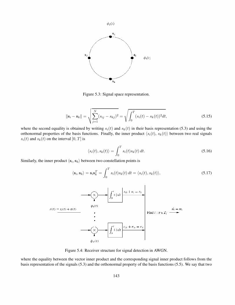
Figure 5.3: Signal space representation.

‖si − sk‖ =

√

√

√

√

N∑

j=1

(sij − skj)2 =

√

∫ T

0(si(t)− sk(t))2dt, (5.15)

where the second equality is obtained by writing si(t) and sk(t) in their basis representation (5.3) and using the

orthonormal properties of the basis functions. Finally, the inner product 〈si(t), sk(t)〉 between two real signals

si(t) and sk(t) on the interval [0, T ] is

〈si(t), sk(t)〉 =

∫ T

0

si(t)sk(t) dt. (5.16)

Similarly, the inner product 〈si, sk〉 between two constellation points is

〈si, sk〉 = sisTk =

∫ T

0

si(t)sk(t) dt = 〈si(t), sk(t)〉, (5.17)

Figure 5.4: Receiver structure for signal detection in AWGN.

where the equality between the vector inner product and the corresponding signal inner product follows from the

basis representation of the signals (5.3) and the orthonormal property of the basis functions (5.5). We say that two

143

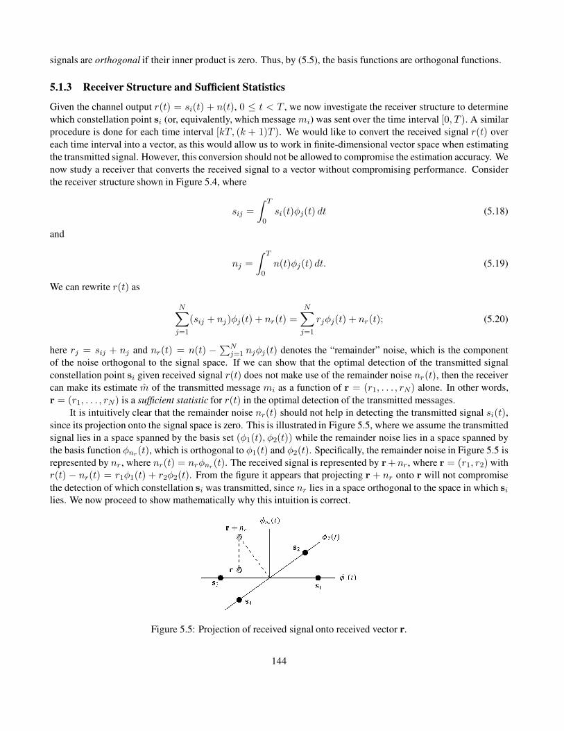
signals are orthogonal if their inner product is zero. Thus, by (5.5), the basis functions are orthogonal functions.

5.1.3 Receiver Structure and Sufficient Statistics

Given the channel output r(t) = si(t) + n(t), 0 ≤ t < T , we now investigate the receiver structure to determine

which constellation point si (or, equivalently, which message mi) was sent over the time interval [0, T ). A similar

procedure is done for each time interval [kT, (k + 1)T ). We would like to convert the received signal r(t) over

each time interval into a vector, as this would allow us to work in finite-dimensional vector space when estimating

the transmitted signal. However, this conversion should not be allowed to compromise the estimation accuracy. We

now study a receiver that converts the received signal to a vector without compromising performance. Consider

the receiver structure shown in Figure 5.4, where

sij =

∫ T

0si(t)φj(t) dt (5.18)

and

nj =

∫ T

0n(t)φj(t) dt. (5.19)

We can rewrite r(t) as

N∑

j=1

(sij + nj)φj(t) + nr(t) =

N∑

j=1

rjφj(t) + nr(t); (5.20)

here rj = sij + nj and nr(t) = n(t) −∑Nj=1 njφj(t) denotes the “remainder” noise, which is the component

of the noise orthogonal to the signal space. If we can show that the optimal detection of the transmitted signal

constellation point si given received signal r(t) does not make use of the remainder noise nr(t), then the receiver

can make its estimate m of the transmitted message mi as a function of r = (r1, . . . , rN) alone. In other words,

r = (r1, . . . , rN) is a sufficient statistic for r(t) in the optimal detection of the transmitted messages.

It is intuitively clear that the remainder noise nr(t) should not help in detecting the transmitted signal si(t),

since its projection onto the signal space is zero. This is illustrated in Figure 5.5, where we assume the transmitted

signal lies in a space spanned by the basis set (φ1(t), φ2(t)) while the remainder noise lies in a space spanned by

the basis function φnr(t), which is orthogonal to φ1(t) and φ2(t). Specifically, the remainder noise in Figure 5.5 is

represented by nr , where nr(t) = nrφnr(t). The received signal is represented by r+nr, where r = (r1, r2) with

r(t) − nr(t) = r1φ1(t) + r2φ2(t). From the figure it appears that projecting r + nr onto r will not compromise

the detection of which constellation si was transmitted, since nr lies in a space orthogonal to the space in which silies. We now proceed to show mathematically why this intuition is correct.

Figure 5.5: Projection of received signal onto received vector r.

144

Let us first examine the distribution of r. Since n(t) is a Gaussian random process, if we condition on

the transmitted signal si(t) then the channel output r(t) = si(t) + n(t) is also a Gaussian random process and

r = (r1, . . . , rN) is a Gaussian random vector. Recall that rj = sij + nj . Thus, conditioned on a transmitted

constellation si, we have that

µrj |si= E[rj|si] = E[sij + nj|sij] = sij (5.21)

(since n(t) has zero mean) and

σrj |si= E[rj − µrj |si

]2 = E[sij + nj − sij |sij]2 = E[n2j ]. (5.22)

Moreover,

Cov[rjrk|si] = E[(rj − µrj )(rk − µrk )|si]= E[njnk]

= E

[∫ T

0n(t)φj(t) dt

∫ T

0n(τ)φk(τ) dτ

]

=

∫ T

0

∫ T

0

E[n(t)n(τ)]φj(t)φk(τ) dt dτ

=

∫ T

0

∫ T

0

N0

2δ(t− τ)φj(t)φk(τ) dt dτ

=N0

2

∫ T

0φj(t)φk(t) dt

=

{

N0/2 j = k,

0 j 6= k,(5.23)

where the last equality follows from the orthonormality of the basis functions. Thus, conditioned on the transmitted

constellation si, the rj are uncorrelated and, since they are Gaussian, they are also independent. Furthermore,

E[n2j ] = N0/2.

We have shown that, conditioned on the transmitted constellation si, rj is a Gauss-distributed random variable

that is independent of rk(k 6= j) with mean sij and variance N0/2. Thus, the conditional distribution of r is given

by

p(r | si sent) =

N∏

j=1

p(rj |mi) =1

(πN0)N/2exp

− 1

N0

N∑

j=1

(rj − sij)2

. (5.24)

It is also straightforward to show that E[rjnr(t) | si] = 0 for any t, 0 ≤ t < T . Thus, since rj conditioned on siand nr(t) are Gaussian and uncorrelated, they are independent. Also, since the transmitted signal is independent

of the noise, sij is independent of the process nr(t).

We now discuss the receiver design criterion and show that it is not affected by discarding nr(t). The goal of

the receiver design is to minimize the probability of error in detecting the transmitted message mi given received

signal r(t). In order to minimize Pe = p(m 6= mi | r(t)) = 1 − p(m = mi | r(t)), we maximize p(m =mi | r(t)). Therefore, the receiver output m given received signal r(t) should correspond to the message mi that

maximizes p(mi sent | r(t)). Since there is a one-to-one mapping between messages and signal constellation

145

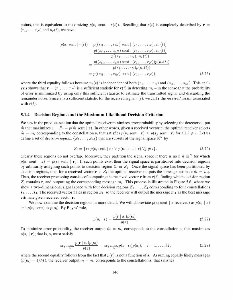
points, this is equivalent to maximizing p(si sent | r(t)). Recalling that r(t) is completely described by r =(r1, . . . , rN) and nr(t), we have

p(si sent | r(t)) = p((si1, . . . , siN ) sent | (r1, . . . , rN), nr(t))

=p((si1, . . . , siN ) sent, (r1, . . . , rN), nr(t))

p((r1, . . . , rN), nr(t))

=p((si1, . . . , siN ) sent, (r1, . . . , rN))p(nr(t))

p(r1, . . . , rN)p(nr(t))

= p((si1, . . . , siN ) sent | (r1, . . . , rN)), (5.25)

where the third equality follows because nr(t) is independent of both (r1, . . . , rN) and (si1, . . . , siN ). This anal-

ysis shows that r = (r1, . . . , rN) is a sufficient statistic for r(t) in detecting mi – in the sense that the probability

of error is minimized by using only this sufficient statistic to estimate the transmitted signal and discarding the

remainder noise. Since r is a sufficient statistic for the received signal r(t), we call r the received vector associated

with r(t).

5.1.4 Decision Regions and the Maximum Likelihood Decision Criterion

We saw in the previous section that the optimal receiver minimizes error probability by selecting the detector output

m that maximizes 1 − Pe = p(m sent | r). In other words, given a received vector r, the optimal receiver selects

m = mi corresponding to the constellation si that satisfies p(si sent | r) ≥ p(sj sent | r) for all j 6= i. Let us

define a set of decision regions {Z1, . . . , ZM} that are subsets of the signal space RN by

Zi = {r : p(si sent | r) > p(sj sent | r) ∀j 6= i}. (5.26)

Clearly these regions do not overlap. Moreover, they partition the signal space if there is no r ∈ RN for which

p(si sent | r) = p(si sent | r). If such points exist then the signal space is partitioned into decision regions

by arbitrarily assigning such points to decision region Zi or Zj . Once the signal space has been partitioned by

decision regions, then for a received vector r ∈ Zi the optimal receiver outputs the message estimate m = mi.

Thus, the receiver processing consists of computing the received vector r from r(t), finding which decision region

Zi contains r, and outputting the corresponding message mi. This process is illustrated in Figure 5.6, where we

show a two-dimensional signal space with four decision regions Z1, . . . , Z4 corresponding to four constellations

s1, . . . , s4. The received vector r lies in region Z1, so the receiver will output the message m1 as the best message

estimate given received vector r.

We now examine the decision regions in more detail. We will abbreviate p(si sent | r received) as p(si | r)

and p(si sent) as p(si). By Bayes’ rule,

p(si | r) =p(r | si)p(si)

p(r). (5.27)

To minimize error probability, the receiver output m = mi corresponds to the constellation si that maximizes

p(si | r); that is, si must satisfy

arg maxsi

p(r | si)p(si)p(r)

= argmaxsi

p(r | si)p(si), i = 1, . . . ,M, (5.28)

where the second equality follows from the fact that p(r) is not a function of si. Assuming equally likely messages

(p(si) = 1/M), the receiver output m = mi corresponds to the constellation si that satisfies

146

Figure 5.6: Decision regions.

argmaxsi

p(r | si), i = 1, . . . ,M. (5.29)

Let us define the likelihood function associated with our receiver as

L(si) = p(r | si). (5.30)

Given a received vector r, a maximum likelihood receiver outputs m = mi corresponding to the constellation

si that maximizes L(si). Since the log function is increasing in its argument, maximizing L(si) is equivalent

to maximizing its log. Moreover, the constant factor (πN0)−N/2 in (5.24) does not affect the maximization of

L(si) relative to si. Thus, maximizing L(si) is equivalent to maximizing the log likelihood function, defined as

l(si) = ln[(πN0)N/2L(si)]. Using (5.24) for L(si) = p(r | si) then yields

Figure 5.7: Matched filter receiver structure.

l(si) = − 1

N0

N∑

j=1

(rj − sij)2 = − 1

N0‖r− si‖2. (5.31)

147

Thus, the log likelihood function l(si) depends only on the distance between the received vector r and the con-

stellation point si. Moreover, from (5.31), l(si) is maximized by the constellation point si that is closest to the

received vector r.

The maximum likelihood receiver is implemented using the structure shown in Figure 5.4. First r is computed

from r(t), and then the signal constellation closest to r is determined as the constellation point si satisfying

argminsi

N∑

j=1

(rj − sij)2 = argmin

si

‖r− si‖2. (5.32)

This si is determined from the decision region Zi that contains r, where Zi is defined by

Zi = {r : ‖r − si‖ < ‖r − sj‖∀j = 1, . . . ,M, j 6= i}, i = 1, . . . ,M. (5.33)

Finally, the estimated constellation si is mapped to the estimated message m, which is output from the receiver.

This result is intuitively satisfying, since the receiver decides that the transmitted constellation point is the one

closest to the received vector. This maximum likelihood receiver structure is simple to implement because the

decision criterion depends only on vector distances. This structure also minimizes the probability of message error

at the receiver output when the transmitted messages are equally likely. However, if the messages and correspond-

ing signal constellatations are not equally likely then the maximum likelihood receiver does not minimize error

probability; in order to minimize error probability, the decision regions Zi must be modified to take into account

the message probabilities, as indicated in (5.27).

An alternate receiver structure is shown in Figure 5.7. This structure makes use of a bank of filters matched

to each of the different basis functions. We call a filter with impulse response ψ(t) = φ(T − t), 0 ≤ t ≤ T , the

matched filter to the signal φ(t), so Figure 5.7 is also called a matched filter receiver. It can be shown that if a

given input signal is passed through a filter matched to that signal then the output SNR is maximized. One can also

show that the sampled matched filter outputs (r1, . . . , rn) in Figure 5.7 are the same as the (r1, . . . , rn) in Figure

5.4, so the receivers depicted in these two figures are equivalent.

Example 5.23: For BPSK modulation, find decision regions Z1 and Z2 corresponding to constellations s1 = A

and s2 = −A for A > 0. Solution: The signal space is one-dimensional, so r = r ∈ R. By (5.33) the decision

region Z1 ⊂ R is defined by

Z1 = {r : ‖r −A‖ < ‖r− (−A)‖} = {r : r > 0}.

Thus, Z1 contains all positive numbers on the real line. Similarly

Z2 = {r : ‖r − (−A)‖ < ‖r −A‖} = {r : r < 0}.

So Z2 contains all negative numbers on the real line. For r = 0 the distance is the same to s1 = A and s2 = −A,

so we arbitrarily assign r = 0 to Z2.

5.1.5 Error Probability and the Union Bound

We now analyze the error probability associated with the maximum likelihood receiver structure. For equally likely

messages p(mi sent) = 1/M , we have

148

Pe =

M∑

i=1

p(r 6∈ Zi | mi sent)p(mi sent)

=1

M

M∑

i=1

p(r 6∈ Zi | mi sent)

= 1 − 1

M

M∑

i=1

p(r ∈ Zi | mi sent)

= 1 − 1

M

M∑

i=1

∫

Zi

p(r | mi) dr

= 1 − 1

M

M∑

i=1

∫

Zi

p(r = si + n | si) dn

= 1 − 1

M

M∑

i=1

∫

Zi−si

p(n) dn. (5.34)

The integrals in (5.34) are over theN -dimensional subset Zi ⊂ RN . We illustrate this error probability calculation

in Figure 5.8, where the constellation points s1, . . . , s8 are equally spaced around a circle with minimum separation

dmin. The probability of correct reception assuming the first symbol is sent, p(r ∈ Z1 | m1 sent), corresponds to

the probability p(r = s1 + n ∈ Z1 | s1) that, when noise is added to the transmitted constellation s1, the resulting

vector r = s1 + n remains in the Z1 region shown by the shaded area.

Figure 5.8 also indicates that the error probability is invariant to an angle rotation or axis shift of the sig-

nal constellation. The right side of the figure indicates a phase rotation of θ and axis shift of P relative to the

constellation on the left side. Thus, s′i = siejθ + P. The rotational invariance follows because the noise vector

n = (n1, . . . , nN ) has components that are i.i.d. Gaussian random variables with zero mean; hence the polar

representation n = |n|ejθ has θ uniformly distributed, so the noise statistics are invariant to a phase rotation. The

shift invariance follows from the fact that, if the constellation is shifted by some value P ∈ RN , then the decision

regions defined by (5.33) are also shifted by P. Let (si, Zi) denote a constellation point and corresponding decision

region before the shift and (s′i, Z′i) the corresponding constellation point and decision region after the shift. It is

then straightforward to show that p(r = si + n ∈ Zi | si) = p(r′ = s′i + n ∈ Z ′i | s′i). Thus, the error probability

after an axis shift of the constellation points will remain unchanged.

Although (5.34) gives an exact solution to the probability of error, we cannot solve for this error probability

in closed form. Therefore, we now investigate the union bound on error probability, which yields a closed-form

expression that is a function of the distance between signal constellation points. Let Aik denote the event that

‖r − sk‖ < ‖r − si‖ given that the constellation point si was sent. If the event Aik occurs, then the constellation

will be decoded in error because the transmitted constellation si is not the closest constellation point to the received

vector r. However, event Aik does not necessarily imply that sk will be decoded instead of si, since there may

be another constellation point sl with ‖r − sl‖ < ‖r − sk‖ < ‖r − si‖. The constellation is decoded correctly if

‖r− si‖ < ‖r− sk‖ for all k 6= i. Thus

Pe(mi sent) = p

M⋃

k=1k 6=i

Aik

≤M∑

k=1k 6=i

p(Aik), (5.35)

149

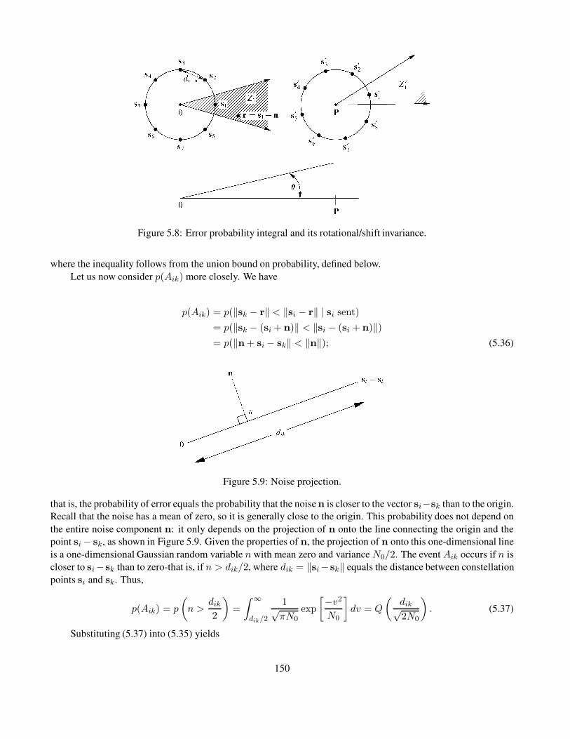
Figure 5.8: Error probability integral and its rotational/shift invariance.

where the inequality follows from the union bound on probability, defined below.

Let us now consider p(Aik) more closely. We have

p(Aik) = p(‖sk − r‖ < ‖si − r‖ | si sent)

= p(‖sk − (si + n)‖ < ‖si − (si + n)‖)= p(‖n + si − sk‖ < ‖n‖); (5.36)

Figure 5.9: Noise projection.

that is, the probability of error equals the probability that the noise n is closer to the vector si−sk than to the origin.

Recall that the noise has a mean of zero, so it is generally close to the origin. This probability does not depend on

the entire noise component n: it only depends on the projection of n onto the line connecting the origin and the

point si− sk, as shown in Figure 5.9. Given the properties of n, the projection of n onto this one-dimensional line

is a one-dimensional Gaussian random variable n with mean zero and variance N0/2. The event Aik occurs if n is

closer to si−sk than to zero-that is, if n > dik/2, where dik = ‖si−sk‖ equals the distance between constellation

points si and sk. Thus,

p(Aik) = p

(

n >dik2

)

=

∫ ∞

dik/2

1√πN0

exp

[−v2

N0

]

dv = Q

(

dik√2N0

)

. (5.37)

Substituting (5.37) into (5.35) yields

150

Pe(mi sent) ≤M∑

k=1k 6=i

Q

(

dik√2N0

)

, (5.38)

where the Q-function, Q(z), is defined as the probability that a Gaussian random variable X with mean 0 and

variance 1 is greater than z:

Q(z) = p(X > z) =

∫ ∞

z

1√2πe−x

2/2dx. (5.39)

Summing (5.38) over all possible messages yields the union bound

Pe =

M∑

i=1

p(mi)Pe(mi sent) ≤ 1

M

M∑

i=1

M∑

k=1k 6=i

Q

(

dik√2N0

)

. (5.40)

Note that the Q-function cannot be solved for in closed form. It is related to the complementary error function as

Q(z) =1

2erfc

(

z√2

)

. (5.41)

We can also place an upper bound on Q(z) with the closed-form expression

Q(z) ≤ 1

z√

2πe−z

2/2, (5.42)

and this bound is tight for z � 0.

Defining the minimum distance of the constellation as dmin = mini,k dik, we can simplify (5.40) with the

looser bound

Pe ≤ (M − 1)Q

(

dmin√2N0

)

. (5.43)

Using (5.42) for the Q-function yields a closed-form bound

Pe ≤M − 1

dmin

√

π/N0

exp

[−d2min

4N0

]

. (5.44)

Finally, Pe is sometimes approximated as the probability of error associated with constellations at the minimum

distance dmin multiplied by the number Mdmin of neighbors at this distance:

Pe ≈MdminQ

(

dmin√2N0

)

. (5.45)

This approximation is called the nearest neighbor approximation to Pe. When different constellation points have a

different number of nearest neighbors or different minimum distances, the bound can be averaged over the bound

associated with each constellation point. Note that the nearest neighbor approximation will always be less than the

loose bound (5.43) since M ≥ Mdmin . It will also be slightly less than the union bound (5.40), since the nearest

neighbor approximation does not include the error associated with constellations farther apart than the minimum

distance. However, the nearest neighbor approximation is quite close to the exact probability of symbol error at

high SNRs, since for x and y large with x > y, Q(x) � Q(y) owing to the exponential falloff of the Gaussian

distribution in (5.39). This indicates that the probability of mistaking a constellation point for another point that

151

is not one of its nearest neighbors is negligible at high SNRs. A rigorous derivation for (5.45) is made in [4] and

also referenced in [5]. Moreover, [4] indicates that (5.45) captures the performance degradation due to imperfect

receiver conditions such as slow carrier drift with an appropriate adjustment of the constants. The appeal of the

nearest neighbor approximation is that it depends only on the minimum distance in the signal constellation and the

number of nearest neighbors for points in the constellation.

Example 5.24: Consider a signal constellation in R2 defined by s1 = (A, 0), s2 = (0, A), s3 = (−A, 0), and

s4 = (0,−A). AssumeA/√N0 = 4. Find the minimum distance and the union bound (5.40), looser bound (5.43),

closed-form bound (5.44), and nearest neighbor approximation (5.45) on Pe for this constellation set. Solution:

The constellation is as depicted in Figure 5.3 with the radius of the circle equal to A. By symmetry, we need

only consider the error probability associated with one of the constellation points, since it will be the same for the

others. We focus on the error associated with transmitting constellation point s1. The minimum distance to this

constellation point is easily computed as dmin = d12 = d23 = d34 = d14 =√A2 + A2 =

√2A2. The distance to

the other constellation points are d13 = d24 = 2A. By symmetry, Pe(mi sent) = Pe(mj sent) for j 6= i, so the

union bound simplifies to

Pe ≤4∑

j=2

Q

(

d1j√2N0

)

= 2Q

(

A√N0

)

+Q

(√2A√N0

)

= 2Q(4) +Q(√

32) = 3.1679 · 10−5.

The looser bound yields

Pe ≤ 3Q(4) = 9.5014 · 10−5,

which is roughly a factor of 3 looser than the union bound. The closed-form bound yields

Pe ≤3

√

2πA2/N0

exp

[−.5A2

N0

]

= 1.004 · 10−4,

which differs from the union bound by about an order of magnitude. Finally, the nearest neighbor approximation

yields

Pe ≈ 2Q(4) = 3.1671 · 10−5,

which (as expected) is approximately equal to the union bound.

Note that, for binary modulation (where M = 2), there is only one way to make an error and dmin is the distance

between the two signal constellation points, so the bound (5.43) is exact:

Pb = Q

(

dmin√2N0

)

. (5.46)

The square of the minimum distance dmin in (5.44) and (5.46) is typically proportional to the SNR of the received

signal, as discussed in Chapter 6.Thus, error probability is reduced by increasing the received signal power.

Recall that Pe is the probability of a symbol (message) error: Pe = p(m 6= mi | mi sent), where mi

corresponds to a message with log2 M bits. However, system designers are typically more interested in the bit

error probability (also called the bit error rate, BER) than in the symbol error probability, because bit errors drive

the performance of higher-layer networking protocols and end-to-end performance. Thus, we would like to design

152

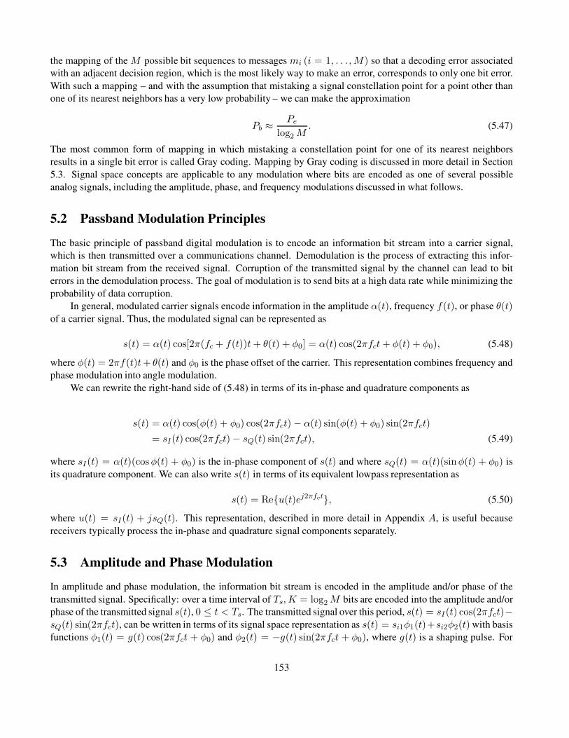
the mapping of the M possible bit sequences to messages mi (i = 1, . . . ,M) so that a decoding error associated

with an adjacent decision region, which is the most likely way to make an error, corresponds to only one bit error.

With such a mapping – and with the assumption that mistaking a signal constellation point for a point other than

one of its nearest neighbors has a very low probability – we can make the approximation

Pb ≈Pe

log2 M. (5.47)

The most common form of mapping in which mistaking a constellation point for one of its nearest neighbors

results in a single bit error is called Gray coding. Mapping by Gray coding is discussed in more detail in Section

5.3. Signal space concepts are applicable to any modulation where bits are encoded as one of several possible

analog signals, including the amplitude, phase, and frequency modulations discussed in what follows.

5.2 Passband Modulation Principles

The basic principle of passband digital modulation is to encode an information bit stream into a carrier signal,

which is then transmitted over a communications channel. Demodulation is the process of extracting this infor-

mation bit stream from the received signal. Corruption of the transmitted signal by the channel can lead to bit

errors in the demodulation process. The goal of modulation is to send bits at a high data rate while minimizing the

probability of data corruption.

In general, modulated carrier signals encode information in the amplitude α(t), frequency f(t), or phase θ(t)

of a carrier signal. Thus, the modulated signal can be represented as

s(t) = α(t) cos[2π(fc + f(t))t+ θ(t) + φ0] = α(t) cos(2πfct+ φ(t) + φ0), (5.48)

where φ(t) = 2πf(t)t+ θ(t) and φ0 is the phase offset of the carrier. This representation combines frequency and

phase modulation into angle modulation.

We can rewrite the right-hand side of (5.48) in terms of its in-phase and quadrature components as

s(t) = α(t) cos(φ(t) + φ0) cos(2πfct) − α(t) sin(φ(t) + φ0) sin(2πfct)

= sI(t) cos(2πfct) − sQ(t) sin(2πfct), (5.49)

where sI(t) = α(t)(cosφ(t) + φ0) is the in-phase component of s(t) and where sQ(t) = α(t)(sinφ(t) + φ0) is

its quadrature component. We can also write s(t) in terms of its equivalent lowpass representation as

s(t) = Re{u(t)ej2πfct}, (5.50)

where u(t) = sI(t) + jsQ(t). This representation, described in more detail in Appendix A, is useful because

receivers typically process the in-phase and quadrature signal components separately.

5.3 Amplitude and Phase Modulation

In amplitude and phase modulation, the information bit stream is encoded in the amplitude and/or phase of the

transmitted signal. Specifically: over a time interval of Ts, K = log2M bits are encoded into the amplitude and/or

phase of the transmitted signal s(t), 0 ≤ t < Ts. The transmitted signal over this period, s(t) = sI(t) cos(2πfct)−sQ(t) sin(2πfct), can be written in terms of its signal space representation as s(t) = si1φ1(t)+si2φ2(t) with basis

functions φ1(t) = g(t) cos(2πfct + φ0) and φ2(t) = −g(t) sin(2πfct + φ0), where g(t) is a shaping pulse. For

153

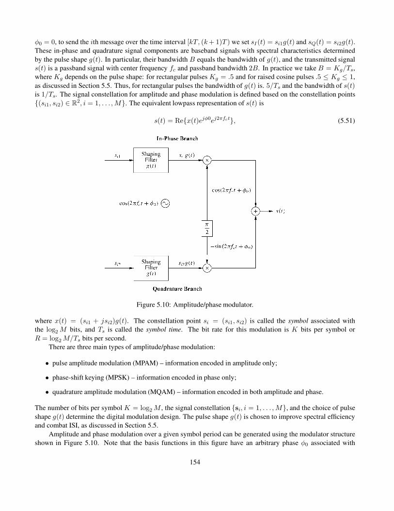
φ0 = 0, to send the ith message over the time interval [kT, (k+ 1)T ) we set sI (t) = si1g(t) and sQ(t) = si2g(t).

These in-phase and quadrature signal components are baseband signals with spectral characteristics determined

by the pulse shape g(t). In particular, their bandwidth B equals the bandwidth of g(t), and the transmitted signal

s(t) is a passband signal with center frequency fc and passband bandwidth 2B. In practice we take B = Kg/Ts,where Kg depends on the pulse shape: for rectangular pulses Kg = .5 and for raised cosine pulses .5 ≤ Kg ≤ 1,

as discussed in Section 5.5. Thus, for rectangular pulses the bandwidth of g(t) is. 5/Ts and the bandwidth of s(t)is 1/Ts. The signal constellation for amplitude and phase modulation is defined based on the constellation points

{(si1, si2) ∈ R2, i = 1, . . . ,M}. The equivalent lowpass representation of s(t) is

s(t) = Re{x(t)ejφ0ej2πfct}, (5.51)

Figure 5.10: Amplitude/phase modulator.

where x(t) = (si1 + jsi2)g(t). The constellation point si = (si1, si2) is called the symbol associated with

the log2 M bits, and Ts is called the symbol time. The bit rate for this modulation is K bits per symbol or

R = log2M/Ts bits per second.

There are three main types of amplitude/phase modulation:

• pulse amplitude modulation (MPAM) – information encoded in amplitude only;

• phase-shift keying (MPSK) – information encoded in phase only;

• quadrature amplitude modulation (MQAM) – information encoded in both amplitude and phase.

The number of bits per symbol K = log2M , the signal constellation {si, i = 1, . . . ,M}, and the choice of pulse

shape g(t) determine the digital modulation design. The pulse shape g(t) is chosen to improve spectral efficiency

and combat ISI, as discussed in Section 5.5.

Amplitude and phase modulation over a given symbol period can be generated using the modulator structure

shown in Figure 5.10. Note that the basis functions in this figure have an arbitrary phase φ0 associated with

154

the transmit oscillator. Demodulation over each symbol period is performed using the demodulation structure

of Figure 5.11, which is equivalent to the structure of Figure 5.7 for φ1(t) = g(t) cos(2πfct + φ) and φ2(t) =

−g(t) sin(2πfct + φ). Typically the receiver includes some additional circuitry for carrier phase recovery that

matches the carrier phase φ at the receiver to the carrier phase φ0 at the transmitter;1 this is known as coherent

detection. If φ−φ0 = 4φ 6= 0 then the in-phase branch will have an unwanted term associated with the quadrature

branch and vice versa; that is, r1 = si1 cos(4φ) + si2 sin(4φ) +n1 and r2 = −si1 sin(4φ) + si2 cos(4φ) + n2,

which can result in significant performance degradation. The receiver structure also assumes that the sampling

function every Ts seconds is synchronized to the start of the symbol period, which is called synchronization or

timing recovery. Receiver synchronization and carrier phase recovery are complex receiver operations that can be

highly challenging in wireless environments. These operations are discussed in more detail in Section 5.6. We will

assume perfect carrier recovery in our discussion of MPAM, MPSK, and MQAM and therefore set φ = φ0 = 0

for their analysis.

Figure 5.11: Amplitude/phase demodulator (coherent: φ = φ0).

5.3.1 Pulse Amplitude Modulation (MPAM)

We will start by looking at the simplest form of linear modulation, one- dimensional MPAM, which has no quadra-

ture component (si2 = 0). For MPAM, all of the information is encoded into the signal amplitude Ai. The

transmitted signal over one symbol time is given by

si(t) = Re{Aig(t)ej2πfct} = Aig(t) cos(2πfct), 0 ≤ t ≤ Ts � 1/fc, (5.52)

where Ai = (2i − 1 − M)d, i = 1, 2, . . . ,M . The signal constellation is thus {Ai, i = 1, . . . ,M}, which is

parameterized by the distance d. This distance is typically a function of the signal energy. The pulse shape g(t)

must satisfy (5.12) and (5.13). The minimum distance between constellation points is dmin = min i,j|Ai −Aj | =2d. The amplitude of the transmitted signal takes on M different values, which implies that each pulse conveys

log2M = K bits per symbol time Ts.Over each symbol period, the MPAM signal associated with the ith constellation has energy

1In fact, an additional phase term of −2πfcτ will result from a propagation delay of τ in the channel. Thus, coherent detection requires

the receiver phase φ = φ0 − 2πfcτ , as discussed in more detail in Section 5.6.

155

Figure 5.12: Gray encoding for MPAM.

Esi =

∫ Ts

0s2i (t) dt =

∫ Ts

0A2i g

2(t) cos2(2πfct) dt = A2i , (5.53)

since the pulse shape must satisfy (5.12).2 Note that the energy is not the same for each signal si(t), i = 1, . . . ,M .

Assuming equally likely symbols, the average energy is

Es =1

M

M∑

i=1

A2i . (5.54)

The constellation mapping is usually done by Gray encoding, where the messages associated with signal

amplitudes that are adjacent to each other differ by one bit value, as illustrated in Figure 5.12. With this encoding

method, if noise causes the demodulation process to mistake one symbol for an adjacent one (the most likely type

of error), the result is only a single bit error in the sequence of K bits. Gray codes can also be designed for MPSK

and square MQAM constellations but not for rectangular MQAM.

Example 5.25: For g(t) =√

2/Ts(0 ≤ t < Ts) a rectangular pulse shape, find the average energy of 4-PAM

modulation. Solution: For 4-PAM the Ai values are Ai = {−3d,−d, d, 3d}, so the average energy is

Es =d2

4(9 + 1 + 1 + 9) = 5d2.

The decision regions Zi, i = 1, . . . ,M , associated with pulse amplitude Ai = (2i − 1 −M)d for M = 4 and

M = 8 are shown in Figure 5.13. Mathematically, for any M these decision regions are defined by

Zi =

(−∞, Ai + d) i = 1,

[Ai − d, Ai + d) 2 ≤ i ≤M − 1,[Ai − d,∞) i = M.

From (5.52) we see that MPAM has only a single basis function φ1(t) = g(t) cos(2πfct). Thus, the coherent

demodulator of Figure 5.11 for MPAM reduces to the demodulator shown in Figure 5.14, where the multithreshold

device maps r to a decision region Zi and outputs the corresponding bit sequence m = mi = {b1, . . . , bK}.

2Recall from (5.8) that (5.12) and hence (5.53) are not exact equalities but rather very good approximations for fcTs � 1.

156

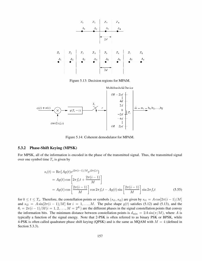
Figure 5.13: Decision regions for MPAM.

Figure 5.14: Coherent demodulator for MPAM.

5.3.2 Phase-Shift Keying (MPSK)

For MPSK, all of the information is encoded in the phase of the transmitted signal. Thus, the transmitted signal

over one symbol time Ts is given by

si(t) = Re{Ag(t)ej2π(i−1)/Mej2πfct}

= Ag(t) cos

[

2πfct+2π(i− 1)

M

]

= Ag(t) cos

[

2π(i− 1)

M

]

cos 2πfct− Ag(t) sin

[

2π(i− 1)

M

]

sin 2πfct (5.55)

for 0 ≤ t ≤ Ts. Therefore, the constellation points or symbols (si1, si2) are given by si1 = A cos[2π(i− 1)/M ]

and si2 = A sin[2π(i − 1)/M ] for i = 1, . . . ,M . The pulse shape g(t) satisfies (5.12) and (5.13), and the

θi = 2π(i− 1)/M(i = 1, 2, . . . ,M = 2K) are the different phases in the signal constellation points that convey

the information bits. The minimum distance between constellation points is dmin = 2A sin(π/M), where A is

typically a function of the signal energy. Note that 2-PSK is often referred to as binary PSK or BPSK, while

4-PSK is often called quadrature phase shift keying (QPSK) and is the same as MQAM with M = 4 (defined in

Section 5.3.3).

157

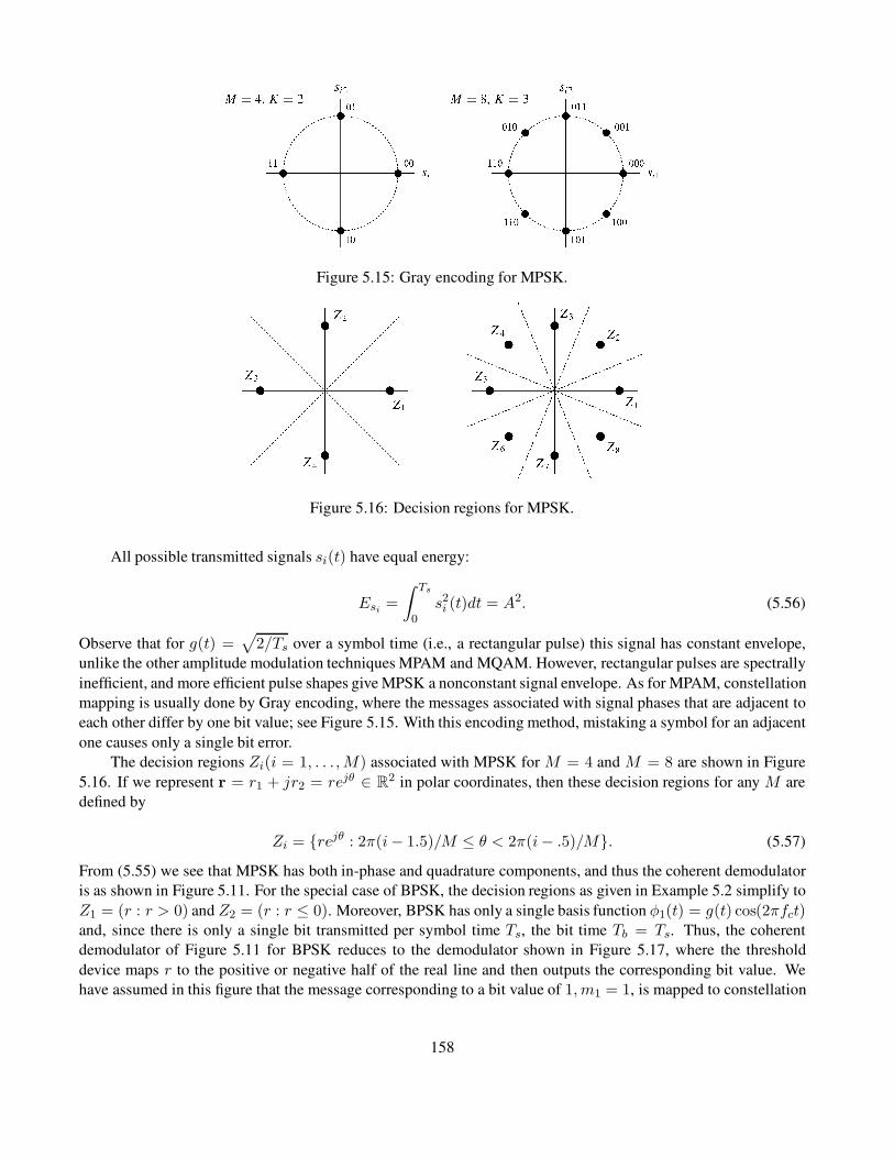
Figure 5.15: Gray encoding for MPSK.

Figure 5.16: Decision regions for MPSK.

All possible transmitted signals si(t) have equal energy:

Esi =

∫ Ts

0s2i (t)dt = A2. (5.56)

Observe that for g(t) =√

2/Ts over a symbol time (i.e., a rectangular pulse) this signal has constant envelope,

unlike the other amplitude modulation techniques MPAM and MQAM. However, rectangular pulses are spectrally

inefficient, and more efficient pulse shapes give MPSK a nonconstant signal envelope. As for MPAM, constellation

mapping is usually done by Gray encoding, where the messages associated with signal phases that are adjacent to

each other differ by one bit value; see Figure 5.15. With this encoding method, mistaking a symbol for an adjacent

one causes only a single bit error.

The decision regions Zi(i = 1, . . . ,M) associated with MPSK for M = 4 and M = 8 are shown in Figure

5.16. If we represent r = r1 + jr2 = rejθ ∈ R2 in polar coordinates, then these decision regions for any M are

defined by

Zi = {rejθ : 2π(i− 1.5)/M ≤ θ < 2π(i− .5)/M}. (5.57)

From (5.55) we see that MPSK has both in-phase and quadrature components, and thus the coherent demodulator

is as shown in Figure 5.11. For the special case of BPSK, the decision regions as given in Example 5.2 simplify to

Z1 = (r : r > 0) and Z2 = (r : r ≤ 0). Moreover, BPSK has only a single basis function φ1(t) = g(t) cos(2πfct)and, since there is only a single bit transmitted per symbol time Ts, the bit time Tb = Ts. Thus, the coherent

demodulator of Figure 5.11 for BPSK reduces to the demodulator shown in Figure 5.17, where the threshold

device maps r to the positive or negative half of the real line and then outputs the corresponding bit value. We

have assumed in this figure that the message corresponding to a bit value of 1, m1 = 1, is mapped to constellation

158

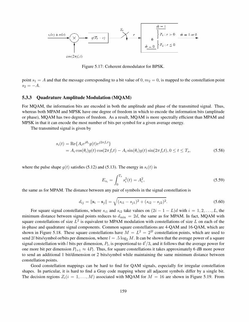
Figure 5.17: Coherent demodulator for BPSK.

point s1 = A and that the message corresponding to a bit value of 0, m2 = 0, is mapped to the constellation point

s2 = −A.

5.3.3 Quadrature Amplitude Modulation (MQAM)

For MQAM, the information bits are encoded in both the amplitude and phase of the transmitted signal. Thus,

whereas both MPAM and MPSK have one degree of freedom in which to encode the information bits (amplitude

or phase), MQAM has two degrees of freedom. As a result, MQAM is more spectrally efficient than MPAM and

MPSK in that it can encode the most number of bits per symbol for a given average energy.

The transmitted signal is given by

si(t) = Re{Aiejθig(t)ej2πfct}= Ai cos(θi)g(t) cos(2πfct) − Ai sin(θi)g(t) sin(2πfct), 0 ≤ t ≤ Ts, (5.58)

where the pulse shape g(t) satisfies (5.12) and (5.13). The energy in si(t) is

Esi =

∫ Ts

0

s2i (t) = A2i , (5.59)

the same as for MPAM. The distance between any pair of symbols in the signal constellation is

dij = ‖si − sj‖ =√

(si1 − sj1)2 + (si2 − sj2)2. (5.60)

For square signal constellations, where si1 and si2 take values on (2i − 1 − L)d with i = 1, 2, . . . , L, the

minimum distance between signal points reduces to dmin = 2d, the same as for MPAM. In fact, MQAM with

square constellations of size L2 is equivalent to MPAM modulation with constellations of size L on each of the

in-phase and quadrature signal components. Common square constellations are 4-QAM and 16-QAM, which are

shown in Figure 5.18. These square constellations have M = L2 = 22l constellation points, which are used to

send 2l bits/symbol or/bits per dimension, where l = .5 log2 M . It can be shown that the average power of a square

signal constellation with l bits per dimension, Pl, is proportional to 4l/3, and it follows that the average power for

one more bit per dimension Pl+1 ≈ 4Pl. Thus, for square constellations it takes approximately 6 dB more power

to send an additional 1 bit/dimension or 2 bits/symbol while maintaining the same minimum distance between

constellation points.

Good constellation mappings can be hard to find for QAM signals, especially for irregular constellation

shapes. In particular, it is hard to find a Gray code mapping where all adjacent symbols differ by a single bit.

The decision regions Zi(i = 1, . . . ,M) associated with MQAM for M = 16 are shown in Figure 5.19. From

159

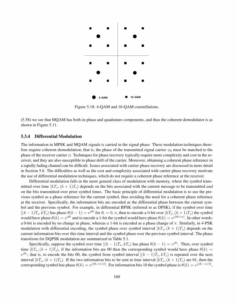
4−QAM 16−QAM

Figure 5.18: 4-QAM and 16-QAM constellations.

(5.58) we see that MQAM has both in-phase and quadrature components, and thus the coherent demodulator is as

shown in Figure 5.11.

5.3.4 Differential Modulation

The information in MPSK and MQAM signals is carried in the signal phase. These modulation techniques there-

fore require coherent demodulation; that is, the phase of the transmitted signal carrier φ0 must be matched to the

phase of the receiver carrier φ. Techniques for phase recovery typically require more complexity and cost in the re-

ceiver, and they are also susceptible to phase drift of the carrier. Moreover, obtaining a coherent phase reference in

a rapidly fading channel can be difficult. Issues associated with carrier phase recovery are discussed in more detail

in Section 5.6. The difficulties as well as the cost and complexity associated with carrier phase recovery motivate

the use of differential modulation techniques, which do not require a coherent phase reference at the receiver.

Differential modulation falls in the more general class of modulation with memory, where the symbol trans-

mitted over time [kTs, (k + 1)Ts) depends on the bits associated with the current message to be transmitted and

on the bits transmitted over prior symbol times. The basic principle of differential modulation is to use the pre-

vious symbol as a phase reference for the current symbol, thus avoiding the need for a coherent phase reference

at the receiver. Specifically, the information bits are encoded as the differential phase between the current sym-

bol and the previous symbol. For example, in differential BPSK (referred to as DPSK), if the symbol over time

[(k− 1)Ts, kTs) has phase θ(k − 1) = ejθi for θi = 0, π, then to encode a 0-bit over [kTs, (k+ 1)Ts) the symbol

would have phase θ(k) = ejθi and to encode a 1-bit the symbol would have phase θ(k) = ej(θi+π). In other words:

a 0-bit is encoded by no change in phase, whereas a 1-bit is encoded as a phase change of π. Similarly, in 4-PSK

modulation with differential encoding, the symbol phase over symbol interval [kTs, (k + 1)Ts) depends on the

current information bits over this time interval and the symbol phase over the previous symbol interval. The phase

transitions for DQPSK modulation are summarized in Table 5.1.

Specifically, suppose the symbol over time [(k − 1)Ts, kTs) has phase θ(k − 1) = ejθi . Then, over symbol

time [kTs, (k + 1)Ts), if the information bits are 00 then the corresponding symbol would have phase θ(k) =ejθi ; that is, to encode the bits 00, the symbol from symbol interval [(k − 1)Ts, kTs) is repeated over the next

interval [kTs, (k + 1)Ts). If the two information bits to be sent at time interval [kTs, (k + 1)Ts) are 01, then the

corresponding symbol has phase θ(k) = ej(θi+π/2). For information bits 10 the symbol phase is θ(k) = ej(θi−π/2),

160

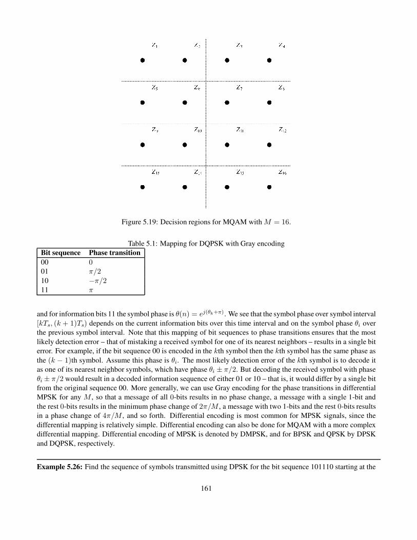
Figure 5.19: Decision regions for MQAM with M = 16.

Table 5.1: Mapping for DQPSK with Gray encoding

Bit sequence Phase transition

00 001 π/2

10 −π/211 π

and for information bits 11 the symbol phase is θ(n) = ej(θk+π). We see that the symbol phase over symbol interval

[kTs, (k + 1)Ts) depends on the current information bits over this time interval and on the symbol phase θi over

the previous symbol interval. Note that this mapping of bit sequences to phase transitions ensures that the most

likely detection error – that of mistaking a received symbol for one of its nearest neighbors – results in a single bit

error. For example, if the bit sequence 00 is encoded in the kth symbol then the kth symbol has the same phase as

the (k − 1)th symbol. Assume this phase is θi. The most likely detection error of the kth symbol is to decode it

as one of its nearest neighbor symbols, which have phase θi ± π/2. But decoding the received symbol with phase

θi ± π/2 would result in a decoded information sequence of either 01 or 10 – that is, it would differ by a single bit

from the original sequence 00. More generally, we can use Gray encoding for the phase transitions in differential

MPSK for any M , so that a message of all 0-bits results in no phase change, a message with a single 1-bit and

the rest 0-bits results in the minimum phase change of 2π/M , a message with two 1-bits and the rest 0-bits results

in a phase change of 4π/M , and so forth. Differential encoding is most common for MPSK signals, since the

differential mapping is relatively simple. Differential encoding can also be done for MQAM with a more complex

differential mapping. Differential encoding of MPSK is denoted by DMPSK, and for BPSK and QPSK by DPSK

and DQPSK, respectively.

Example 5.26: Find the sequence of symbols transmitted using DPSK for the bit sequence 101110 starting at the

161

kth symbol time, assuming the transmitted symbol at the (k − 1)th symbol time was s(k − 1) = Aejπ .

Solution: The first bit, a 1, results in a phase transition of π, so s(k) = A. The next bit, a 0, results in no transition,

so s(k + 1) = A. The next bit, a 1, results in another transition of π, so s(k + 1) = Aejπ , and so on. The full

symbol sequence corresponding to 101110 is A,A, Aejπ, A, Aejπ, Aejπ.

The demodulator for differential modulation is shown in Figure 5.20. Assume the transmitted constellation at time

k is s(k) = Aej(θ(k)+(φ0). Then the received vector associated with the sampler outputs is

r(k) = r1(k) + jr2(k) = Aej(θ(k)+(φ0) + n(k), (5.61)

where n(k) is complex white Gaussian noise. The received vector at the previous time sample k − 1 is thus

r(k− 1) = r1(k − 1) + jr2(k − 1) = Aej(θ(k−1)+(φ0) + n(k − 1). (5.62)

The phase difference between r(k) and r(k− 1) determines which symbol was transmitted. Consider

r(k)r∗(k − 1) =A2ej(θ(k)−θ(k−1)) +Aej(θ(k)+φ0)n∗(k − 1)

+ Ae−j(θ(k−1)+φ0)n(k) + n(k)n∗(k − 1). (5.63)

In the absence of noise (n(k) = n(k − 1) = 0) only the first term in (5.63) is nonzero, and this term yields

the desired phase difference. The phase comparator in Figure 5.20 extracts this phase difference and outputs the

corresponding symbol.

Differential modulation is less sensitive to a random drift in the carrier phase. However, if the channel has

a nonzero Doppler frequency then the signal phase can decorrelate between symbol times, making the previous

symbol a noisy phase reference. This decorrelation gives rise to an irreducible error floor for differential modulation

over wireless channels with Doppler, as we shall discuss in Chapter 6.

Figure 5.20: Differential PSK demodulator.

162

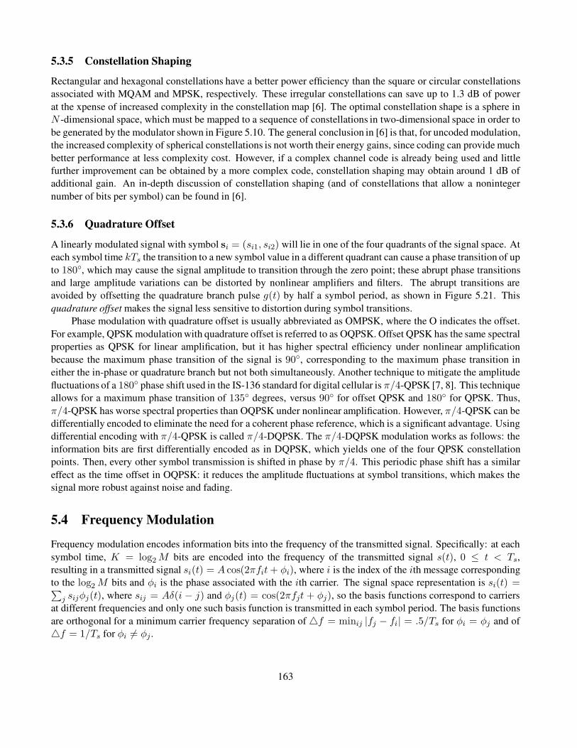
5.3.5 Constellation Shaping

Rectangular and hexagonal constellations have a better power efficiency than the square or circular constellations

associated with MQAM and MPSK, respectively. These irregular constellations can save up to 1.3 dB of power

at the xpense of increased complexity in the constellation map [6]. The optimal constellation shape is a sphere in

N -dimensional space, which must be mapped to a sequence of constellations in two-dimensional space in order to

be generated by the modulator shown in Figure 5.10. The general conclusion in [6] is that, for uncoded modulation,

the increased complexity of spherical constellations is not worth their energy gains, since coding can provide much

better performance at less complexity cost. However, if a complex channel code is already being used and little

further improvement can be obtained by a more complex code, constellation shaping may obtain around 1 dB of

additional gain. An in-depth discussion of constellation shaping (and of constellations that allow a noninteger

number of bits per symbol) can be found in [6].

5.3.6 Quadrature Offset

A linearly modulated signal with symbol si = (si1, si2) will lie in one of the four quadrants of the signal space. At

each symbol time kTs the transition to a new symbol value in a different quadrant can cause a phase transition of up

to 180◦, which may cause the signal amplitude to transition through the zero point; these abrupt phase transitions

and large amplitude variations can be distorted by nonlinear amplifiers and filters. The abrupt transitions are

avoided by offsetting the quadrature branch pulse g(t) by half a symbol period, as shown in Figure 5.21. This

quadrature offset makes the signal less sensitive to distortion during symbol transitions.

Phase modulation with quadrature offset is usually abbreviated as OMPSK, where the O indicates the offset.

For example, QPSK modulation with quadrature offset is referred to as OQPSK. Offset QPSK has the same spectral

properties as QPSK for linear amplification, but it has higher spectral efficiency under nonlinear amplification

because the maximum phase transition of the signal is 90◦, corresponding to the maximum phase transition in

either the in-phase or quadrature branch but not both simultaneously. Another technique to mitigate the amplitude

fluctuations of a 180◦ phase shift used in the IS-136 standard for digital cellular is π/4-QPSK [7, 8]. This technique

allows for a maximum phase transition of 135◦ degrees, versus 90◦ for offset QPSK and 180◦ for QPSK. Thus,

π/4-QPSK has worse spectral properties than OQPSK under nonlinear amplification. However, π/4-QPSK can be

differentially encoded to eliminate the need for a coherent phase reference, which is a significant advantage. Using

differential encoding with π/4-QPSK is called π/4-DQPSK. The π/4-DQPSK modulation works as follows: the

information bits are first differentially encoded as in DQPSK, which yields one of the four QPSK constellation

points. Then, every other symbol transmission is shifted in phase by π/4. This periodic phase shift has a similar

effect as the time offset in OQPSK: it reduces the amplitude fluctuations at symbol transitions, which makes the

signal more robust against noise and fading.

5.4 Frequency Modulation

Frequency modulation encodes information bits into the frequency of the transmitted signal. Specifically: at each

symbol time, K = log2M bits are encoded into the frequency of the transmitted signal s(t), 0 ≤ t < Ts,resulting in a transmitted signal si(t) = A cos(2πfit+ φi), where i is the index of the ith message corresponding

to the log2 M bits and φi is the phase associated with the ith carrier. The signal space representation is si(t) =∑

j sijφj(t), where sij = Aδ(i − j) and φj(t) = cos(2πfjt + φj), so the basis functions correspond to carriers

at different frequencies and only one such basis function is transmitted in each symbol period. The basis functions

are orthogonal for a minimum carrier frequency separation of 4f = minij |fj − fi| = .5/Ts for φi = φj and of

4f = 1/Ts for φi 6= φj .

163

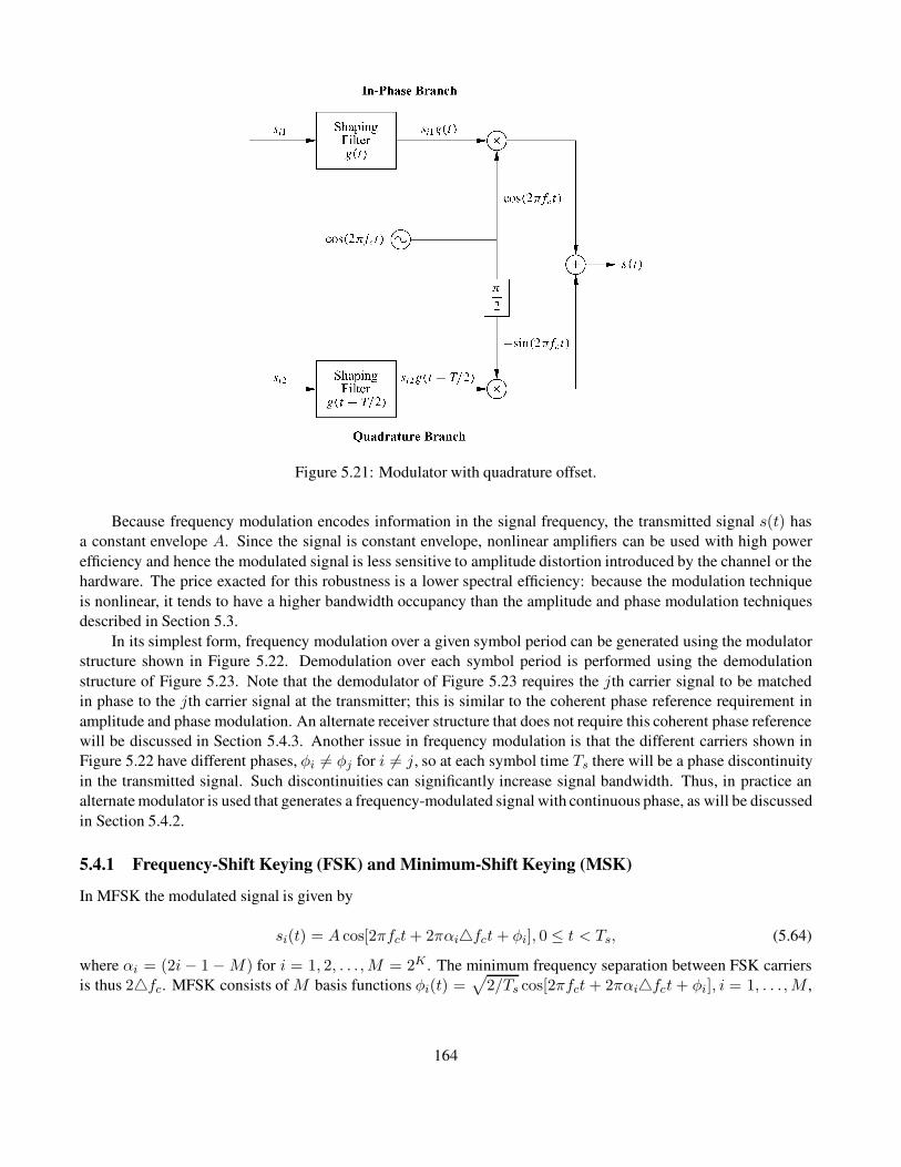
Figure 5.21: Modulator with quadrature offset.

Because frequency modulation encodes information in the signal frequency, the transmitted signal s(t) has

a constant envelope A. Since the signal is constant envelope, nonlinear amplifiers can be used with high power

efficiency and hence the modulated signal is less sensitive to amplitude distortion introduced by the channel or the

hardware. The price exacted for this robustness is a lower spectral efficiency: because the modulation technique

is nonlinear, it tends to have a higher bandwidth occupancy than the amplitude and phase modulation techniques

described in Section 5.3.

In its simplest form, frequency modulation over a given symbol period can be generated using the modulator

structure shown in Figure 5.22. Demodulation over each symbol period is performed using the demodulation

structure of Figure 5.23. Note that the demodulator of Figure 5.23 requires the jth carrier signal to be matched

in phase to the jth carrier signal at the transmitter; this is similar to the coherent phase reference requirement in

amplitude and phase modulation. An alternate receiver structure that does not require this coherent phase reference

will be discussed in Section 5.4.3. Another issue in frequency modulation is that the different carriers shown in

Figure 5.22 have different phases, φi 6= φj for i 6= j, so at each symbol time Ts there will be a phase discontinuity

in the transmitted signal. Such discontinuities can significantly increase signal bandwidth. Thus, in practice an

alternate modulator is used that generates a frequency-modulated signal with continuous phase, as will be discussed

in Section 5.4.2.

5.4.1 Frequency-Shift Keying (FSK) and Minimum-Shift Keying (MSK)

In MFSK the modulated signal is given by

si(t) = A cos[2πfct+ 2παi4fct+ φi], 0 ≤ t < Ts, (5.64)

where αi = (2i− 1 −M) for i = 1, 2, . . . ,M = 2K . The minimum frequency separation between FSK carriers

is thus 24fc. MFSK consists of M basis functions φi(t) =√

2/Ts cos[2πfct+ 2παi4fct+ φi], i = 1, . . . ,M ,

164

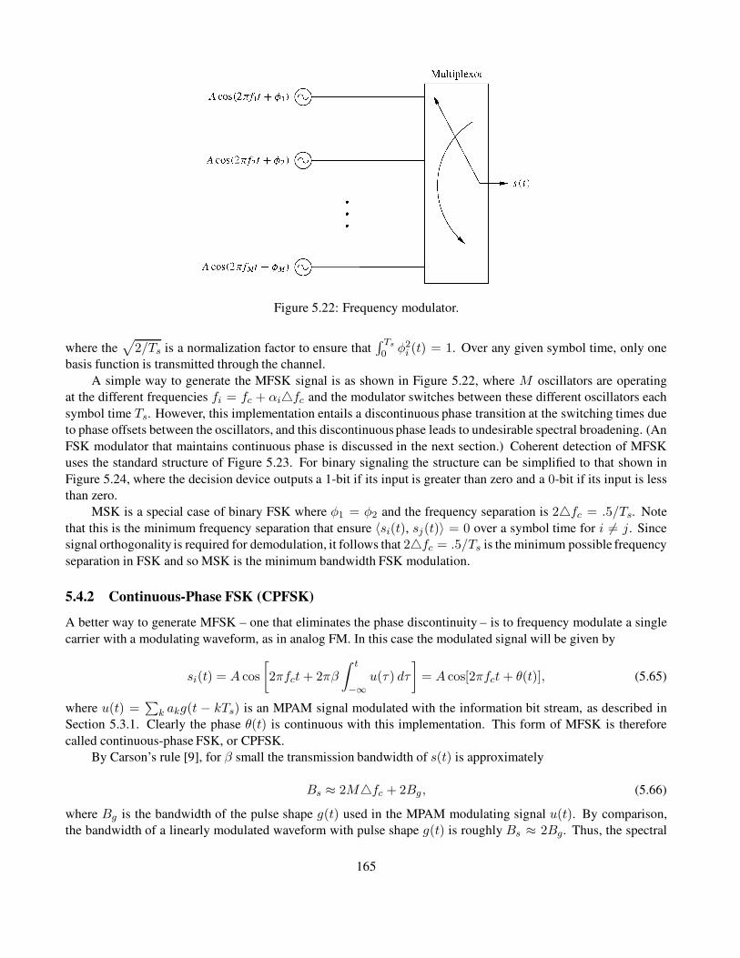
Figure 5.22: Frequency modulator.

where the√

2/Ts is a normalization factor to ensure that∫ Ts

0 φ2i (t) = 1. Over any given symbol time, only one

basis function is transmitted through the channel.

A simple way to generate the MFSK signal is as shown in Figure 5.22, where M oscillators are operating

at the different frequencies fi = fc + αi4fc and the modulator switches between these different oscillators each

symbol time Ts. However, this implementation entails a discontinuous phase transition at the switching times due

to phase offsets between the oscillators, and this discontinuous phase leads to undesirable spectral broadening. (An

FSK modulator that maintains continuous phase is discussed in the next section.) Coherent detection of MFSK

uses the standard structure of Figure 5.23. For binary signaling the structure can be simplified to that shown in

Figure 5.24, where the decision device outputs a 1-bit if its input is greater than zero and a 0-bit if its input is less

than zero.

MSK is a special case of binary FSK where φ1 = φ2 and the frequency separation is 24fc = .5/Ts. Note

that this is the minimum frequency separation that ensure 〈si(t), sj(t)〉 = 0 over a symbol time for i 6= j. Since

signal orthogonality is required for demodulation, it follows that 24fc = .5/Ts is the minimum possible frequency

separation in FSK and so MSK is the minimum bandwidth FSK modulation.

5.4.2 Continuous-Phase FSK (CPFSK)

A better way to generate MFSK – one that eliminates the phase discontinuity – is to frequency modulate a single

carrier with a modulating waveform, as in analog FM. In this case the modulated signal will be given by

si(t) = A cos

[

2πfct+ 2πβ

∫ t

−∞

u(τ) dτ

]

= A cos[2πfct+ θ(t)], (5.65)

where u(t) =∑

k akg(t − kTs) is an MPAM signal modulated with the information bit stream, as described in

Section 5.3.1. Clearly the phase θ(t) is continuous with this implementation. This form of MFSK is therefore

called continuous-phase FSK, or CPFSK.

By Carson’s rule [9], for β small the transmission bandwidth of s(t) is approximately

Bs ≈ 2M4fc + 2Bg , (5.66)

where Bg is the bandwidth of the pulse shape g(t) used in the MPAM modulating signal u(t). By comparison,

the bandwidth of a linearly modulated waveform with pulse shape g(t) is roughly Bs ≈ 2Bg. Thus, the spectral

165

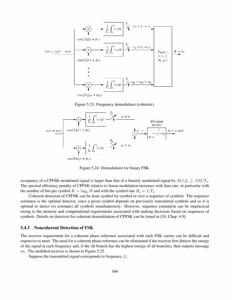
Figure 5.23: Frequency demodulator (coherent).

Figure 5.24: Demodulator for binary FSK.

occupancy of a CPFSK-modulated signal is larger than that of a linearly modulated signal by M4fc ≥ .5M/Ts.The spectral efficiency penalty of CPFSK relative to linear modulation increases with data rate, in particular with

the number of bits per symbol K = log2 M and with the symbol rate Rs = 1/Ts.Coherent detection of CPFSK can be done symbol-by-symbol or over a sequence of symbols. The sequence

estimator is the optimal detector, since a given symbol depends on previously transmitted symbols and so it is

optimal to detect (or estimate) all symbols simultaneously. However, sequence estimation can be impractical

owing to the memory and computational requirements associated with making decisions based on sequences of

symbols. Details on detectors for coherent demodulation of CPFSK can be found in [10, Chap. 4.9].

5.4.3 Noncoherent Detection of FSK

The receiver requirement for a coherent phase reference associated with each FSK carrier can be difficult and

expensive to meet. The need for a coherent phase reference can be eliminated if the receiver first detects the energy

of the signal at each frequency and, if the ith branch has the highest energy of all branches, then outputs message

mi. The modified receiver is shown in Figure 5.25.

Suppose the transmitted signal corresponds to frequency fi:

166

s(t) = A cos(2πfit+ φi)

= A cos(φi) cos(2πfit) − A sin(φi) sin(2πfit), 0 ≤ t < Ts. (5.67)

Let the phase φi represent the phase offset between the transmitter and receiver oscillators at frequency fi. A

coherent receiver with carrier signal cos(2πfit) detects only the first term A cos(φi) cos(2πfit) associated with

the received signal, which can be close to zero for a phase offset φi ≈ ±π/2. To get around this problem, in Figure

5.25 the receiver splits the received signal intoM branches corresponding to each frequency fj , j = 1, . . . ,M . For

each such carrier frequency fj , the received signal is multiplied by a noncoherent in-phase and quadrature carrier

at that frequency, integrated over a symbol time, sampled, and then squared. For the jth branch the squarer output

associated with the in-phase component is denoted as AjI + njI and the corresponding output associated with the

quadrature component is denoted as AjQ + njQ, where njI and njQ are due to the noise n(t) at the receiver input.

Then, if i = j, we have AjI = A2 cos2(φi) and AjQ = A2 sin2(φi); if i 6= j then AjI = AjQ = 0. In the absence

of noise, the input to the decision device of the ith branch will beA2 cos2(φi)+A2 sin2(φi) = A2, independent of

φi, and all other branches will have an input of zero. Thus, over each symbol period, the decision device outputs

the bit sequence corresponding to frequency fj if the jth branch has the largest input to the decision device. Note

that the noncoherent receiver of Figure 5.25 still requires accurate synchronization for sampling. Synchronization

issues are discussed in Section 5.6.

Figure 5.25: Noncoherent FSK demodulator.

5.5 Pulse Shaping

For amplitude and phase modulation, the bandwidth of the baseband and passband modulated signal is a function

of the bandwidth of the pulse shape g(t). If g(t) is a rectangular pulse of width Ts, then the envelope of the signal is

constant. However, a rectangular pulse has high spectral sidelobes, which can cause adjacent channel interference.

Pulse shaping is a method for reducing sidelobe energy relative to a rectangular pulse; however, the shaping must

167

be done in such a way that intersymbol interference between pulses in the received signal is not introduced. Note

that – prior to sampling the received signal – the transmitted pulse g(t) is convolved with the channel impulse

response c(t) and the matched filter g∗(−t); hence, in order to eliminate ISI prior to sampling, we must ensure that

the effective received pulse p(t) = g(t) ∗ c(t) ∗ g∗(−t) has no ISI. Since the channel model is AWGN, we assume

c(t) = δ(t) so p(t) = g(t) ∗ g∗(−t) (in Chapter 11we will analyze ISI for more general channel impulse responses

c(t)). To avoid ISI between samples of the received pulses, the effective pulse shape p(t) must satisfy the Nyquist

criterion, which requires the pulse to equal zero at the ideal sampling point associated with past or future symbols:

p(kTs) =

{

p0 = p(0) k = 0,0 k 6= 0.

In the frequency domain this translates to

∞∑

l=−∞

P

(

f +l

Ts

)

= p0Ts. (5.68)

The following pulse shapes all satisfy the Nyquist criterion.

1. Rectangular pulses: g(t) =√

2/Ts(0 ≤ t ≤ Ts), which yields the triangular effective pulse shape

p(t) =

2 + 2t/Ts −Ts ≤ t < 0,2 − 2t/Ts 0 ≤ t < Ts,

0 else.

This pulse shape leads to constant envelope signals in MPSK but has poor spectral properties as a result of

its high sidelobes.

2. Cosine pulses: p(t) = sinπt/Ts, 0 ≤ t ≤ Ts. Cosine pulses are mostly used in OMPSK modulation,

where the quadrature branch of the modulation is shifted in time by Ts/2. This leads to a constant amplitude

modulation with sidelobe energy that is 10 dB lower than that of rectangular pulses.

3. Raised cosine pulses: These pulses are designed in the frequency domain according to the desired spectral

properties. Thus, the pulse p(t) is first specified relative to its Fourier transform:

P (f) =

{

Ts 0 ≤ |f | ≤ 1−β2Ts

,Ts

2

[

1− sin πTs

β

(

f − 12Ts

)]

1−β2Ts

≤ |f | ≤ 1+β2Ts

;

here β is defined as the rolloff factor, which determines the rate of spectral rolloff (see Figure 5.26). Setting

β = 0 yields a rectangular pulse. The pulse p(t) in the time domain corresponding to P (f) is

p(t) =sinπt/Tsπt/Ts

cosβπt/Ts1 − 4β2t2/T 2

s

.

The frequency- and time-domain properties of the raised cosine pulse are shown in Figures 5.26 and 5.27, respec-

tively. The tails of this pulse in the time domain decay as 1/t3 (faster than for the previous pulse shapes), so a

mistiming error in sampling leads to a series of inter- symbol interference components that converge. A variation

of the raised cosine pulse is the root cosine pulse, derived by taking the square root of the frequency response for

the raised cosine pulse. The root cosine pulse has better spectral properties than the raised cosine pulse but decays

168

Figure 5.26: Frequency-domain (spectral) properties of the raised cosine pulse (T = Ts).

less rapidly in the time domain, which makes performance degradation due to synchronization errors more severe.

Specifically, a mistiming error in sampling leads to a series of ISI components that may diverge.

Pulse shaping is also used with CPFSK to improve spectral efficiency, specifically in the MPAM signal that is

frequency modulated to form the FSK signal. The most common pulse shape used in CPFSK is the Gaussian pulse

shape, defined as

g(t) =

√π

αe−π

2t2/α2, (5.69)

where α is a parameter that dictates spectral efficiency. The spectrum of g(t), which dictates the spectrum of the

CPFSK signal, is given by

G(f) = e−α2f2. (5.70)

The parameter α is related to the 3-dB bandwidth of g(t), Bg, by

α =.5887

Bg. (5.71)

Clearly, increasing α results in a higher spectral efficiency.

When the Gaussian pulse shape is applied to MSK modulation, it is abbreviated as GMSK. In general, GMSK

signals have a high power efficiency (since they have a constant amplitude) and a high spectal efficiency (since

the Gaussian pulse shape has good spectral properties for large α). For these reasons, GMSK is used in the

GSM standard for digital cellular systems. Although this is a good choice for voice modulation, it is not the best

choice for data. The Gaussian pulse shape does not satisfy the Nyquist criterion and so the pulse shape introduces

ISI, which increases as α increases. Thus, improving spectral efficiency by increasing α leads to a higher ISI

level, thereby creating an irreducible error floor from this self-interference. Since the required BER for voice is a

relatively high Pb ≈ 10−3, the ISI can be fairly high and still maintain this target BER. In fact, it is generally used

as a rule of thumb thatBgTs = .5 is a tolerable amount of ISI for voice transmission with GMSK. However, a much

lower BER is required for data, which will put more stringent constraints on the maximum α and corresponding

169

Figure 5.27: Time-domain properties of the raised cosine pulse (T = Ts).

minimum Bg, thereby decreasing the spectral efficiency of GMSK for data transmission. Techniques such as

equalization can be used to mitigate the ISI in this case so that a tolerable BER is possible without significantly

compromising spectral efficiency. However, it is more common to use linear modulation for spectrally efficient

data transmission. Indeed, the data enhancements to GSM use linear modulation.

5.6 Symbol Synchronization and Carrier Phase Recovery

One of the most challenging tasks of a digital demodulator is to acquire accurate symbol timing and carrier phase

information. Timing information, obtained via synchronization, is needed to delineate the received signal asso-

ciated with a given symbol. In particular, timing information is used to drive the sampling devices associated

with the demodulators for amplitude, phase, and frequency demodulation shown in Figures 5.11 and 5.23. Carrier

phase information is needed in all coherent demodulators for both amplitude/phase and frequency modulation, as

discussed in Sections 5.3 and 5.4.

This section gives a brief overview of standard techniques for synchronization and carrier phase recovery in

AWGN channels. In this context the estimation of symbol timing and carrier phase falls under the broader category

of signal parameter estimation in noise. Estimation theory provides the theoretical framework for studying this

problem and for developing the maximum likelihood estimator of the carrier phase and symbol timing. However,

most wireless channels suffer from time-varying multipath in addition to AWGN. Synchronization and carrier

phase recovery is particularly challenging in such channels because multipath and time variations can make it

extremely difficult to estimate signal parameters prior to demodulation. Moreover, there is little theory addressing

good methods for estimation of carrier phase and symbol timing when these parameters are corrupted by time-

varying multipath in addition to noise. In most performance analysis of wireless communication systems it is

assumed that the receiver synchronizes to the multipath component with delay equal to the average delay spread;3

then the channel is treated as AWGN for recovery of timing information and carrier phase. In practice, however, the

receiver will sychronize to either the strongest multipath component or the first multipath component that exceeds

a given power threshold. The other multipath components will then compromise the receiver’s ability to acquire

3That is why delay spread is typically characterized by its rms value about its mean, as discussed in more detail in Chapter 2.

170

timing and carrier phase, especially in wideband systems like UWB. Multicarrier and spread-spectrum systems

have additional considerations related to synchronization and carrier recovery, which will be discussed in Chapters

12 and 13.

The importance of synchronization and carrier phase estimation cannot be overstated: without them, wireless

systems could not function. Moreover, as data rates increase and channels become more complex by adding

additional degrees of freedom (e.g., multiple antennas), the tasks of receiver synchronizaton and phase recovery

become even more complex and challenging. Techniques for synchronization and carrier recovery have been

developed and analyzed extensively for many years, and they are continually evolving to meet the challenges

associated with higher data rates, new system requirements, and more challenging channel characteristics. We give

only a brief introduction to synchronizaton and carrier phase recovery techniques in this section. Comprehensive

coverage of this topic and performance analysis of these techniques can be found in [11, 12]; more condensed

treatments can be found in [bib5-10, Chap. 5;bib5-13].

5.6.1 Receiver Structure with Phase and Timing Recovery

The carrier phase and timing recovery circuitry for the amplitude and phase demodulator is shown in Figure 5.28.

For BPSK only the in-phase branch of this demodulator is needed. For the coherent frequency demodulator of

Figure 5.23, a carrier phase recovery circuit is needed for each of the distinct M carriers; the resulting circuit

complexity motivates the need for noncoherent demodulators as described in Section 5.4.3. We see in Figure 5.28

that the carrier phase and timing recovery circuits operate directly on the received signal prior to demodulation.

Assuming an AWGN channel, the received signal r(t) is a delayed version of the transmitted signal s(t) plus

AWGN n(t) : r(t) = s(t − τ) + n(t), where τ is the random propagation delay. Using the equivalent lowpass

form we have s(t) = Re{x(t)ejφ0ej2πfct} and thus

r(t) = Re{

x(t− τ)ejφej2πfct}

+ n(t), (5.72)

Figure 5.28: Receiver structure with carrier and timing recovery.

where φ = φ0−2πfcτ results from the transmit carrier phase and the propagation delay. Estimation of τ is needed

for symbol timing, and estimation of φ is needed for carrier phase recovery. Let us express these two unknown

171

parameters as a vector ψ = (φ, τ). Then we can express the received signal in terms of ψ as

r(t) = s(t;ψ) + n(t). (5.73)

Parameter estimation must take place over some finite time interval T0 ≥ Ts. We call T0 the observation interval.

In practice, however, parameter estimation is initially done over this interval and is thereafter performed continually

by updating the initial estimate using tracking loops. Our development here focuses on the initial parameter

estimation over T0. Discussion of parameter tracking can be found in [11, 12].

There are two common estimation methods for signal parameters in noise: the maximum likelihood (ML)

criterion discussed in Section 5.1.4 in the context of receiver design, and the maximum a posteriori (MAP) criterion.

The ML criterion chooses the estimate ψ that maximizes p(r(t)|ψ) over the observation interval T0, whereas the

MAP criterion assumes some probability distribution p(ψ) on ψ and then chooses the estimate ψ that maximizes

p(ψ|r(t)) =p(r(t)|ψ)p(ψ)

p(r(t))

over T0. We assume that there is no prior knowledge of ψ, so that p(ψ) becomes uniform and hence the MAP and

ML criteria are equivalent.

To characterize the distribution p(r(t)|ψ), 0 ≤ t < T0, let us expand r(t) over the observation interval along

a set of orthonormal basis functions {φk(t)} as

r(t) =

K∑

k=1

rkφk(t), 0 ≤ t < T0.

Because n(t) is white with zero mean and power spectral density N0/2, the distribution of the vector r =(r1, . . . , rK) conditioned on the unknown parameter ψ is given by

p(r|ψ) =

(

1√πN0

)K

exp

[

−K∑

k=1

(rk − sk(ψ))2

N0

]

, (5.74)

where (by the basis expansion)

rk =

∫

T0

r(t)φk(t) dt

and

sk(ψ) =

∫

T0

s(t;ψ)φk(t) dt.

From these basis expansions we can show that

K∑

k=1

[rk − sk(ψ)]2 =

∫

T0

[r(t)− s(t;ψ)]2 dt. (5.75)

Using this in (5.74) yields that maximizing p(r|ψ) is equivalent to maximizing the likelihood function

Λ(ψ) = exp

[

− 1

N0

∫

T0

[r(t)− s(t;ψ)]2]

dt. (5.76)

172

Maximizing the likelihood function (5.76) results in the joint ML estimate of the carrier phase and symbol

timing. Maximum likelihood estimation of the carrier phase and symbol timing can also be done separately, and in

subsequent sections we will discuss this separate estimation in more detail. Techniques joint estimation are more

complex; details of such techniques can be found in [10, Chap. 6.4; 11, Chaps. 8–9].

5.6.2 Maximum Likelihood Phase Estimation

In this section we derive the maximum likelihood phase estimate assuming the timing is known. The likelihood

function (5.76) with timing known reduces to

Λ(φ) = exp

[

− 1

N0

∫

T0

[r(t)− s(t; φ)]2 dt

]

= exp

[

− 1

N0

∫

T0

x2(t) dt+2

N0

∫

T0

r(t)s(t; φ) dt− 1

N0

∫

T0

s2(t; φ) dt

]

. (5.77)

We estimate the carrier phase as the value φ that maximizes this function. Note that the first term in (5.77) is

independent of φ. Moreover, we assume that the third integral, which measures the energy in s(t; φ) over the

observation interval, is relatively constant in φ. Given these assumptions, we see that the φ that maximizes (5.77)

also maximizes

Figure 5.29: Phase-locked loop for carrier phase recovery (unmodulated carrier).

Λ′(φ) =

∫

T0

r(t)s(t; φ) dt. (5.78)

We can solve directly for the maximizing φ in the simple case where the received signal is just an unmodulated

carrier plus noise: r(t) = A cos(2πfct+ φ) + n(t). Then φ must maximize

Λ′(φ) =

∫

T0

r(t) cos(2πfct+ φ) dt. (5.79)

Differentiating Λ′(φ) relative to φ and then setting it to zero yields that φ satisfies

∫

T0

r(t) sin(2πfct+ φ) dt = 0. (5.80)

Solving (5.80) for φ yields

φ = − tan−1

[∫

T0r(t) sin(2πfct) dt

∫

T0r(t) cos(2πfct) dt

]

. (5.81)

173

We could build a circuit to compute (5.81) from the received signal r(t); in practice, however, carrier phase

recovery is accomplished by using a phase lock loop to satisfy (5.80), as shown in Figure 5.29. In this figure, the

integrator input in the absence of noise is given by e(t) = r(t) sin(2πfct+ φ) and the integrator output is

z(t) =

∫

T0

r(t) sin(2πfct+ φ)dt,

which is precisely the left-hand side of (5.80). Thus, if z(t) = 0 then the estimate φ is the maximum likelihood

estimate for φ. If z(t) 6= 0 then the voltage-controlled oscillator (VCO) adjusts its phase estimate φ up or down

depending on the polarity of z(t): for z(t) > 0 it decreases φ to reduce z(t), and for z(t) < 0 it increases φ to

increase z(t). In practice the integrator in Figure 5.29 is replaced with a loop filter whose output .5A sin(φ−φ) ≈.5A(φ− φ) is a function of the low-frequency component of its input e(t) = A cos(2πfct+ φ) sin(2πfct+ φ) =.5A sin(φ − φ) + .5A sin(2πfct + φ + φ). This discussion of phase-locked loop (PLL) operation assumes that

φ ≈ φ because otherwise the polarity of z(t) may not indicate the correct phase adjustment; that is, we would not

necessarily have sin(φ−φ) ≈ φ−φ. The PLL typically exhibits some transient behavior in its initial estimation of

the carrier phase. The advantage of a PLL is that it continually adjusts its estimate φ to maintain z(t) ≈ 0, which

corrects for slow phase variations due to oscillator drift at the transmitter or changes in the propagation delay. In

fact, the PLL is an example of a feedback control loop. More details on the PLL and its performance can be found

in [10, 11].

The PLL derivation is for an unmodulated carrier, yet amplitude and phase modulation embed the message

bits into the amplitude and phase of the carrier. For such signals there are two common carrier phase recovery

approaches to deal with the effect of the data sequence on the received signal: the data sequence is either (a)

assumed known or (b) treated as random with the phase estimate averaged over the data statistics. The first

scenario is referred to as decision-directed parameter estimation, and this scenario typically results from sending

a known training sequence. The second scenario is referred to as non-decision directed parameter estimation.

With this technique the likelihood function (5.77) is maximized by averaging over the statistics of the data. One

decision-directed technique uses data decisions to remove the modulation of the received signal: the resulting

unmodulated carrier is then passed through a PLL. This basic structure is called a decision-feedback PLL because

data decisions are fed back into the PLL for processing. The structure of a non–decision-directed carrier phase

recovery loop depends on the underlying distribution of the data. For large constellations, most distributions

lead to highly nonlinear functions of the parameter to be estimated. In this case the symbol distribution is often

assumed to be Gaussian along each signal dimension, which greatly simplifies the recovery loop structure. An

alternate non–decision-directed structure takes the M th power of the signal (M = 2 for PAM and M for MPSK

modulation), passes it through a bandpass filter at frequency Mfc, and then uses a PLL. The nonlinear operation

removes the effect of the amplitude or phase modulation so that the PLL can operate on an unmodulated carrier at

frequency Mfc. Many other structures for both decision-directed and non–decision-directed carrier recovery can

be used, with different trade-offs in performance and complexity. A more comprehensive discussion of design and

performance of carrier phase recovery can be found in [10, Chaps. 6.2.4–6.2.5; 11].

5.6.3 Maximum Likelihood Timing Estimation

In this section we derive the maximum likelihood estimate of delay τ assuming the carrier phase is known. Since

we assume that the phase φ is known, the timing recovery will not affect the carrier phase recovery loop and

associated downconversion shown in Figure 5.28. Thus, it suffices to consider timing estimation for the in-phase

or quadrature equivalent lowpass signals of r(t) and s(t; τ). We denote the in-phase and quadrature components

for r(t) as rI(t) and rQ(t) and for s(t; τ) as sI(t; τ) and sQ(t; τ). We focus on the in-phase branch since the

timing recovered from this branch can be used for the quadrature branch. The equivalent lowpass in-phase signal

is given by

174

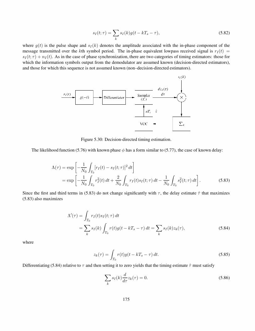
sI(t; τ) =∑

k

sI (k)g(t− kTs − τ), (5.82)

where g(t) is the pulse shape and sI (k) denotes the amplitude associated with the in-phase component of the

message transmitted over the kth symbol period. The in-phase equivalent lowpass received signal is rI(t) =sI(t; τ) + nI(t). As in the case of phase synchronization, there are two categories of timing estimators: those for

which the information symbols output from the demodulator are assumed known (decision-directed estimators),

and those for which this sequence is not assumed known (non–decision-directed estimators).

Figure 5.30: Decision-directed timing estimation.

The likelihood function (5.76) with known phase φ has a form similar to (5.77), the case of known delay:

Λ(τ) = exp

[

− 1

N0

∫

T0

[rI(t)− sI(t; τ)]2 dt

]

= exp

[

− 1

N0

∫

T0

r2I (t) dt+2

N0

∫

T0

rI(t)sI(t; τ) dt−1

N0

∫

T0

s2I (t; τ) dt

]

. (5.83)

Since the first and third terms in (5.83) do not change significantly with τ , the delay estimate τ that maximizes

(5.83) also maximizes

Λ′(τ) =

∫

T0

rI(t)sI(t; τ) dt

=∑

k

sI(k)

∫

T0

r(t)g(t− kTs − τ) dt =∑

k

sI (k)zk(τ), (5.84)

where

zk(τ) =

∫

T0

r(t)g(t− kTs − τ) dt. (5.85)

Differentiating (5.84) relative to τ and then setting it to zero yields that the timing estimate τ must satisfy

∑

k

sI(k)d

dτzk(τ) = 0. (5.86)

175

For decision-directed estimation, (5.86) gives rise to the estimator shown in Figure 5.30. The input to the

voltage-controlled clock (VCC) is (5.86). If this input is zero, then the timing estimate τ = τ . If not, the clock

(i.e., the timing estimate τ ) is adjusted to drive the VCC input to zero. This timing estimation loop is also an

example of a feedback control loop.

One structure for non–decision-directed timing estimation is the early–late gate synchronizer shown in Figure

5.31. This structure exploits two properties of the autocorrelation of g(t),Rg(τ) =∫ TS

0 g(t)g(t−τ) dt – namely, its

symmetry (Rg(τ) = Rg(−τ)) and the fact that its maximum value is at τ = 0. The input to the sampler in the upper

branch of Figure 5.31 is proportional to the autocorrelationRg(τ−τ+δ) =∫ TS

0 g(t−τ)g(t−τ−δ) dt, and the input

to the sampler in the lower branch is proportional to the autocorrelationRg(τ−τ−δ) =∫ TS

0 g(t−τ)g(t−τ+δ)dt.

If τ = τ then, sinceRg(δ) = Rg(−δ), the input to the loop filter will be zero and the voltage-controlled clock will

maintain its correct timing estimate. If τ > τ then Rg(τ − τ + δ) < Rg(τ − τ − δ), and this negative input to the

VCC will cause it to decrease its estimate of τ . Conversely, if τ < τ then Rg(τ − τ + δ) > Rg(τ − τ − δ), and

this positive input to the VCC will cause it to increase its estimate of τ .

Figure 5.31: Early-late gate synchronizer.

More details on these and other structures for decision-directed and non–decision-directed timing estimation–

as well as their performance trade-offs–can be found in [10, Chaps. 6.2.4–6.2.5; 11].

176

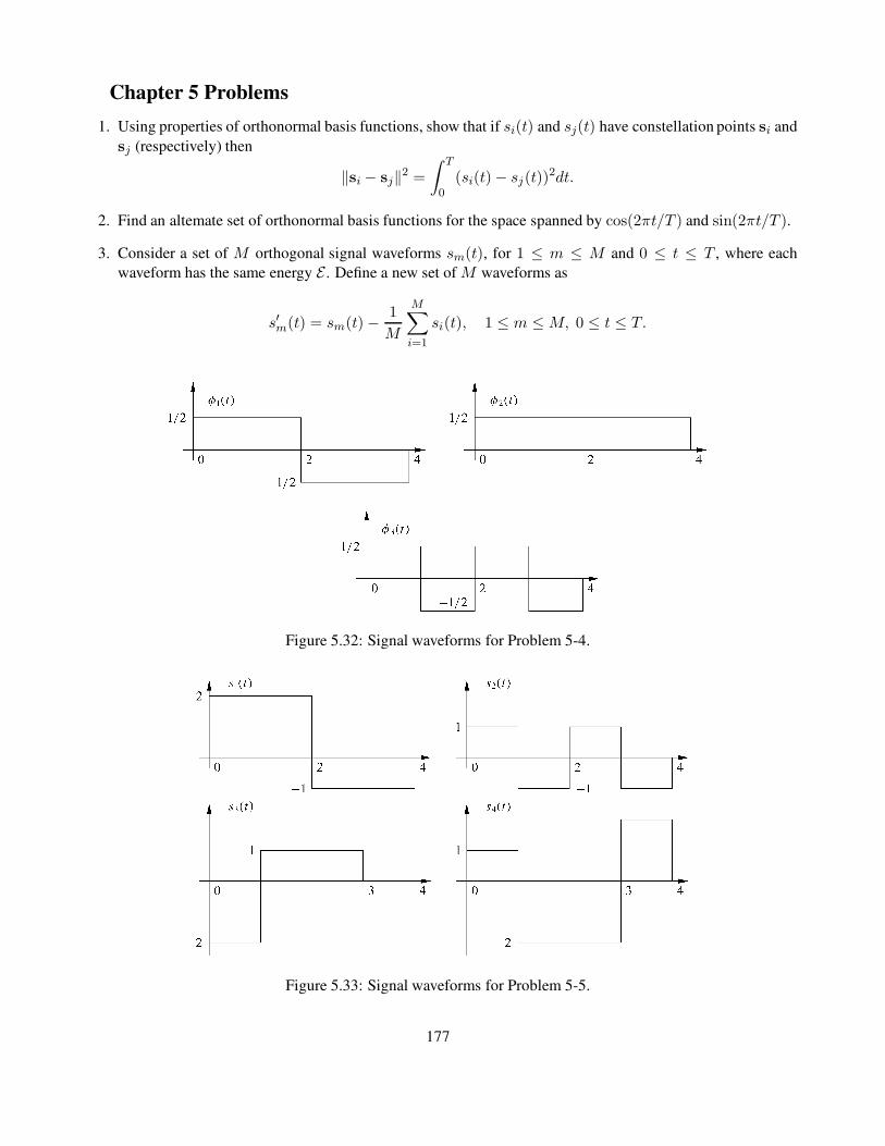
Chapter 5 Problems

1. Using properties of orthonormal basis functions, show that if si(t) and sj(t) have constellation points si and

sj (respectively) then

‖si − sj‖2 =

∫ T

0(si(t) − sj(t))

2dt.

2. Find an altemate set of orthonormal basis functions for the space spanned by cos(2πt/T ) and sin(2πt/T ).

3. Consider a set of M orthogonal signal waveforms sm(t), for 1 ≤ m ≤ M and 0 ≤ t ≤ T , where each

waveform has the same energy E . Define a new set of M waveforms as

s′m(t) = sm(t) − 1

M

M∑

i=1

si(t), 1 ≤ m ≤M, 0 ≤ t ≤ T.

Figure 5.32: Signal waveforms for Problem 5-4.

Figure 5.33: Signal waveforms for Problem 5-5.

177

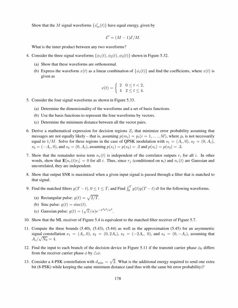
Show that the M signal waveforms {s′m(t)} have equal energy, given by

E ′ = (M − 1)E/M.

What is the inner product between any two waveforms?

4. Consider the three signal waveforms {φ1(t), φ2(t), φ3(t)} shown in Figure 5.32.

(a) Show that these waveforms are orthonormal.

(b) Express the waveform x(t) as a linear combination of {φi(t)} and find the coefficients, where x(t) is

given as

x(t) =

{

2 0 ≤ t < 2,

4 2 ≤ t ≤ 4.

5. Consider the four signal waveforms as shown in Figure 5.33.

(a) Determine the dimensionality of the waveforms and a set of basis functions.

(b) Use the basis functions to represent the four waveforms by vectors.

(c) Determine the minimum distance between all the vector pairs.

6. Derive a mathematical expression for decision regions Zi that minimize error probability assuming that

messages are not equally likely – that is, assuming p(mi) = pi(i = 1, . . . ,M), where pi is not necessarily

equal to 1/M . Solve for these regions in the case of QPSK modulation with s1 = (Ac, 0), s2 = (0, Ac),

s3 = (−Ac, 0), and s4 = (0, Ac), assuming p(s1) = p(s3) = .2 and p(s1) = p(s3) = .3.

7. Show that the remainder noise term nr(t) is independent of the correlator outputs ri for all i. In other

words, show that E[nr(t)ri] = 0 for all i. Thus, since rj (conditioned on si) and nr(t) are Gaussian and

uncorrelated, they are independent.

8. Show that output SNR is maximized when a given input signal is passed through a filter that is matched to

that signal.

9. Find the matched filters g(T − t), 0 ≤ t ≤ T , and Find∫ T0 g(t)g(T − t) dt for the following waveforms.

(a) Rectangular pulse: g(t) =√

2/T .

(b) Sinc pulse: g(t) = sinc(t).

(c) Gaussian pulse: g(t) = (√π/α)e−π

2t2/α2.

10. Show that the ML receiver of Figure 5.4 is equivalent to the matched filter receiver of Figure 5.7.

11. Compute the three bounds (5.40), (5.43), (5.44) as well as the approximation (5.45) for an asymmetric

signal constellation s1 = (Ac, 0), s2 = (0, 2Ac), s3 = (−2Ac, 0), and s4 = (0,−Ac), assuming that

Ac/√N0 = 4.

12. Find the input to each branch of the decision device in Figure 5.11 if the transmit carrier phase φ0 differs

from the receiver carrier phase φ by 4φ.

13. Consider a 4-PSK constellation with dmin =√

2. What is the additional energy required to send one extra

bit (8-PSK) while keeping the same minimum distance (and thus with the same bit error probability)?

178

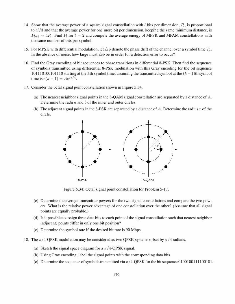
14. Show that the average power of a square signal constellation with l bits per dimension, Pl, is proportional

to 4l/3 and that the average power for one more bit per dimension, keeping the same minimum distance, is

Pl+1 ≈ 4Pl. Find Pl for l = 2 and compute the average energy of MPSK and MPAM constellations with

the same number of bits per symbol.

15. For MPSK with differential modulation, let 4φ denote the phase drift of the channel over a symbol time Ts.In the absence of noise, how large must 4φ be in order for a detection error to occur?

16. Find the Gray encoding of bit sequences to phase transitions in differential 8-PSK. Then find the sequence

of symbols transmitted using differential 8-PSK modulation with this Gray encoding for the bit sequence

101110100101110 starting at the kth symbol time, assuming the transmitted symbol at the (k−1)th symbol

time is s(k − 1) = Aejπ/4.

17. Consider the octal signal point constellation shown in Figure 5.34.

(a) The nearest neighbor signal points in the 8-QAM signal constellation are separated by a distance of A.

Determine the radii a and b of the inner and outer circles.

(b) The adjacent signal points in the 8-PSK are separated by a distance ofA. Determine the radius r of the

circle.

Figure 5.34: Octal signal point constellation for Problem 5-17.

(c) Determine the average transmitter powers for the two signal constellations and compare the two pow-

ers. What is the relative power advantage of one constellation over the other? (Assume that all signal

points are equally probable.)

(d) Is it possible to assign three data bits to each point of the signal constellation such that nearest neighbor

(adjacent) points differ in only one bit position?

(e) Determine the symbol rate if the desired bit rate is 90 Mbps.

18. The π/4-QPSK modulation may be considered as two QPSK systems offset by π/4 radians.

(a) Sketch the signal space diagram for a π/4-QPSK signal.

(b) Using Gray encoding, label the signal points with the corresponding data bits.

(c) Determine the sequence of symbols transmitted via π/4-QPSK for the bit sequence 0100100111100101.

179

(d) Repeat part (c) for π/4-DQPSK, assuming that the last symbol transmitted on the in-phase branch had

a phase of π and that the last symbol transmitted on the quadrature branch had a phase of −3π/4.

19. Show that the minimum frequency separation for FSK such that the cos(2πfjt) and cos(2πfit) are orthog-

onal is 4f = minij |fj − fi| = .5/Ts.

20. Show that the Nyquist criterion for zero ISI pulses given by p(kTs) = p0δ(k) is equivalent to the frequency

domain condition (5.68).

21. Show that the Gaussian pulse shape does not satisfy the Nyquist criterion.

180

Bibliography

[1] S. Haykin and M. Moher, Communication Systems, 5th ed., Wiley, New York, 2009.

[2] J. Proakis and M. Salehi, Communication Systems Engineering, 2nd ed., Pearson, 2001.

[3] J. M. Wozencraft and I. M. Jacobs, Principles of Communication Engineering, Wiley, New York, 1965.

[4] M. Fitz, “Further results in the unified analysis of digital communication systems,” IEEE Trans. Commun.,

pp. 521–32, March 1992.

[5] R. Ziemer, “An overview of modulation and coding for wireless communications,” Proc. IEEE Veh. Tech.

Conf., pp. 26–30, April 1996.

[6] G. D. Forney, Jr., and L.-F. Wei, “Multidimensional constellations-Part I: Introduction, figures of merit, and

generalized cross constellations,” IEEE J. Sel. Areas Commun., pp. 877–92, August 1989.

[7] T. S. Rappaport, Wireless Communications – Principles and Practice, 2nd ed., Prentice-Hall, Englewood

Cliffs, NJ, 2001.

[8] G. L. Stuber, Principles of Mobile Communications, 4th ed., Springer, 2017.

[9] S. Haykin and M. Moher, An Introduction to Analog and Digital Communications, 2nd ed., Wiley, New York,

2006.

[10] J. G. Proakis and M. Salehi, Digital Communications, 5th ed., McGraw-Hill, New York, 2007.

[11] U. Mengali and A. N. D’Andrea, Synchronization Techniques for Digital Receivers, Plenum, New York, 1997.

[12] H. Meyr, M. Moeneclaey, and S. A. Fechtel, Digital Communication Receivers, vol. 2, Synchronization,

Channel Estimation, and Signal Processing, Wiley, New York, 1997.

[13] L. E. Franks, “Carrier and bit synchronization in data communication – A tutorial review,” IEEE Trans.

Commun., pp. 1107–21, August 1980.

181

Chapter 6

Performance of Digital Modulation over

Wireless Channels

We now consider the performance of the digital modulation techniques discussed in the previous chapter when used

over AWGN channels and channels with flat fading. There are two performance criteria of interest: the probability

of error, defined relative to either symbol or bit errors; and the outage probability, defined as the probability that

the instantaneous signal-to-noise ratio falls below a given threshold. Flat fading can cause a dramatic increase

in either the average bit error probability or the signal outage probability. Wireless channels may also exhibit

frequency-selective fading and Doppler shift. Frequency-selective fading gives rise to intersymbol interference

(ISI), which causes an irreducible error floor in the received signal. Doppler causes spectral broadening, which

leads to adjacent channel interference (small at typical user velocities) and also to an irreducible error floor in

signals with differential phase encoding (e.g. DPSK), since the phase reference of the previous symbol partially

decorrelates over a symbol time. This chapter describes the impact on digital modulation performance of noise,

flat fading, frequency-selective fading, and Doppler.

6.1 AWGN Channels

In this section we define the signal-to-noise power ratio (SNR) and its relation to energy per bit (Eb) and energy

per symbol (Es). We then examine the error probability on AWGN channels for different modulation techniques

as parameterized by these energy metrics. Our analysis uses the signal space concepts of Section 5.1.

6.1.1 Signal-to-Noise Power Ratio and Bit/Symbol Energy

In an AWGN channel the modulated signal s(t) = Re{u(t)ej2πfct} has noise n(t) added to it prior to reception.

The noise n(t) is a white Gaussian random process with mean zero and power spectral density (PSD) N0/2. The

received signal is thus r(t) = s(t) + n(t).

We define the received SNR as the ratio of the received signal power Pr to the power of the noise within the

bandwidth of the transmitted signal s(t). The received power Pr is determined by the transmitted power and the

path loss, shadowing, and multipath fading, as described in Chapters 2 and 3. The noise power is determined by

the bandwidth of the transmitted signal and the spectral properties of n(t). Specifically, if the bandwidth of the

complex envelope u(t) of s(t) is B then the bandwidth of the transmitted signal s(t) is 2B. Since the noise n(t)has uniform PSD N0/2, the total noise power within the bandwidth 2B is N = N0/2 · 2B = N0B. Hence the

received SNR is given by

182

SNR =PrN0B

.

In systems with interference, we often use the received signal-to-interference-plus-noise power ratio (SINR) in

place of SNR for calculating error probability. This is a reasonable approximation if the interference statistics

approximate those of Gaussian noise. The received SINR is given by

SINR =Pr

N0B + PI,

where PI is the average power of the interference.

The SNR is often expressed in terms of the signal energy per bit Eb (or per symbol, Es) as

SNR =PrN0B

=Es

N0BTs=

EbN0BTb

, (6.1)

where Ts is the symbol time and Tb is the bit time (for binary modulation Ts = Tb and Es = Eb). For pulse

shaping with Ts = 1/B (e.g., raised consine pluses with β = 1), we have SNR = Es/N0 for multilevel signaling

and SNR = Eb/N0 for binary signaling. For general pulses, Ts = k/B for some constant k, in which case

k · SNR = Es/N0.

The quantities γs = Es/N0 and γb = Eb/N0 are sometimes called the SNR per symbol and the SNR per

bit, respectively. For performance specification, we are interested in the bit error probability Pb as a function of

γb. However, with M -ary signaling (e.g., MPAM and MPSK) the bit error probability depends on both the symbol

error probability and the mapping of bits to symbols. Thus, we typically compute the symbol error probability Psas a function of γs based on the signal space concepts of Section 5.1 and then obtain Pb as a function of γb using an

exact or approximate conversion. The approximate conversion typically assumes that the symbol energy is divided

equally among all bits and that Gray encoding is used, so that (at reasonable SNRs) one symbol error corresponds

to exactly one bit error. These assumptions for M -ary signaling lead to the approximations

γb ≈γs

log2M(6.2)

and

Pb ≈Ps

log2 M. (6.3)

6.1.2 Error Probability for BPSK and OPSK

We first consider BPSK modulation with coherent detection and perfect recovery of the carrier frequency and

phase. With binary modulation each symbol corresponds to one bit, so the symbol and bit error rates are the same.

The transmitted signal is s1(t) = Ag(t) cos(2πfct) to send a 0-bit and s2(t) = −Ag(t) cos(2πfct) to send a 1-bit

for A > 0. From (5.46) we have that the probability of error is

Pb = Q

(

dmin√2N0

)

. (6.4)

From Section 5.3.2, dmin = ‖s1 − s0‖ = ‖A− (−A)‖ = 2A. Let us now relate A to the energy per bit. We have

Eb =

∫ Tb

0s21(t) dt =

∫ Tb

0s22(t) dt =

∫ Tb

0A2g2(t) cos2(2πfct) dt = A2 (6.5)

183

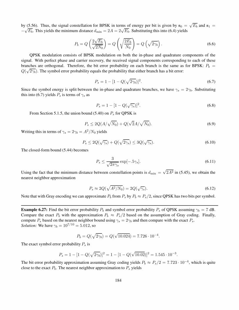
by (5.56). Thus, the signal constellation for BPSK in terms of energy per bit is given by s0 =√Eb and s1 =

−√Eb. This yields the minimum distance dmin = 2A = 2

√Eb. Substituting this into (6.4) yields

Pb = Q

(

2√Eb√

2N0

)

= Q

(

√

2EbN0

)

= Q(

√

2γb

)

. (6.6)

QPSK modulation consists of BPSK modulation on both the in-phase and quadrature components of the

signal. With perfect phase and carrier recovery, the received signal components corresponding to each of these

branches are orthogonal. Therefore, the bit error probability on each branch is the same as for BPSK: Pb =

Q(√

2γb). The symbol error probability equals the probability that either branch has a bit error:

Ps = 1 − [1 −Q(√

2γb)]2. (6.7)

Since the symbol energy is split between the in-phase and quadrature branches, we have γs = 2γb. Substituting

this into (6.7) yields Ps is terms of γs as

Ps = 1 − [1−Q(√γs)]

2. (6.8)

From Section 5.1.5, the union bound (5.40) on Ps for QPSK is

Ps ≤ 2Q(A/√

N0) +Q(√

2A/√

N0). (6.9)

Writing this in terms of γs = 2γb = A2/N0 yields

Ps ≤ 2Q(√γs) +Q(

√

2γs) ≤ 3Q(√γs). (6.10)

The closed-form bound (5.44) becomes

Ps ≤3√

2πγsexp[−.5γs]. (6.11)

Using the fact that the minimum distance between constellation points is dmin =√

2A2 in (5.45), we obtain the

nearest neighbor approximation

Ps ≈ 2Q(√

A2/N0) = 2Q(√γs). (6.12)

Note that with Gray encoding we can approximate Pb from Ps by Pb ≈ Ps/2, since QPSK has two bits per symbol.

Example 6.27: Find the bit error probability Pb and symbol error probability Ps of QPSK assuming γb = 7 dB.

Compare the exact Pb with the approximation Pb ≈ Ps/2 based on the assumption of Gray coding. Finally,

compute Ps based on the nearest neighbor bound using γs = 2γb and then compare with the exact Ps.Solution: We have γb = 107/10 = 5.012, so

Pb = Q(√

2γb) = Q(√

10.024) = 7.726 · 10−4.

The exact symbol error probabilityPs is

Ps = 1 − [1−Q(√

2γb)]2 = 1 − [1 −Q(

√10.02)]2 = 1.545 · 10−3.

The bit error probability approximation assuming Gray coding yields Pb ≈ Ps/2 = 7.723 · 10−4, which is quite

close to the exact Pb. The nearest neighbor approximation to Ps yields

184

Ps ≈ 2Q(√γs) = 2Q(

√10.024) = 1.545 · 10−3,

which matches well with the exact Ps.

6.1.3 Error Probability for MPSK

The signal constellation for MPSK has si1 = A cos[2π(i− 1)/M ] and si2 = A sin[2π(i− 1)/M ] for A > 0 and

i = 1, . . . ,M . The symbol energy is Es = A2, so γs = A2/N0. From (5.57) it follows that, for the received vector

r = rejθ represented in polar coordinates, an error occurs if the ith signal constellation point is transmitted and

θ 6∈ (2π(i− 1 − .5)/M, 2π(i− 1 + .5)/M). The joint distribution of r and θ can be obtained through a bivariate

transformation of the noise n1 and n2 on the in-phase and quadrature branches [1, Chap. 5.2.7], which yields

p(r, θ) =r

πN0exp

[

− 1

N0(r2 − 2

√

Esr cos(θ) + Es)

]

. (6.13)

Since the error probability depends only on the distribution of θ, we can integrate out the dependence on r to obtain

p(θ) =

∫ ∞

0p(r, θ) dr =

1

2πe−γs sin2(θ)

∫ ∞

0z exp

[

−(z −√2γs cos(θ))2

2

]

dz. (6.14)

By symmetry, the probability of error is the same for each constellation point. Thus, we can derive Ps from the

probability of error assuming the constellation point s1 = (A, 0) is transmitted, which is

Ps = 1−∫ π/M

−π/Mp(θ)dθ

= 1−∫ π/M

−π/M

1

2πe−γs sin2(θ)

∫ ∞

0z exp

[

−(z −√2γs cos(θ))2

2

]

dz. (6.15)

A closed-form solution to this integral does not exist for M > 4 and so the exact value of Ps must be computed

numerically.

Each point in the MPSK constellation has two nearest neighbors at distance dmin = 2A sin(π/M). Thus, the

nearest neighbor approximation (5.45) to Ps is given by

Ps ≈ 2Q(√

2A sin(π/M)/√

N0) = 2Q(√

2γs sin(π/M)). (6.16)

This nearest neighbor approximation can differ significantly from the exact value of Ps. However, it is much

simpler to compute than the numerical integration of (6.15) that is required to obtain the exact Ps. This formula

can also be obtained by approximating p(θ) as

p(θ) ≈√

γs/π cos(θ)e−γs sin2(θ). (6.17)

Using this in the first line of (6.15) yields (6.16).

Example 6.28: Compare the probability of bit error for 8-PSK and 16-PSK assuming γb = 15 dB and using the

Ps approximation given in (6.16) along with the approximations (6.3) and (6.2).

Solution: From (6.2) we have that, for 8-PSK, γs = (log2 8) · 1015/10 = 94.87. Substituting this into (6.16) yields

185

Ps ≈ 2Q(√

189.74 sin(π/8)) = 1.355 · 10−7. (6.18a)

Now, using (6.3), we get Pb = Ps/3 = 4.52 · 10−8. For 16-PSK we have γs = (log2 16) · 1015/10 = 126.49.

Substituting this into (6.16) yields

Ps ≈ 2Q(√

252.98 sin(π/16)) = 1.916 · 10−3, (6.18b)

and by using (6.3) we get Pb = Ps/4 = 4.79 · 10−4. Note that Pb is much larger for 16-PSK than for 8-PSK given

the same γb. This result is expected because 16-PSK packs more bits per symbol into a given constellation and so,

for a fixed energy per bit, the minimum distance between constellation points will be smaller.

The error probability derivation for MPSK assumes that the carrier phase is perfectly known to the receiver. Under

phase estimation error, the distribution of p(θ) used to obtain Ps must incorporate the distribution of the phase

rotation associated with carrier phase offset. This distribution is typically a function of the carrier phase estimation

technique and the SNR. The impact of phase estimation error on coherent modulation is studied in [1, Apx. C; 2,

Chap. 4.3.2; 3; 4]. These works indicate that, as expected, significant phase offset leads to an irreducible bit error

probability. Moreover, nonbinary signaling is more sensitive than BPSK to phase offset because of the resulting

cross-coupling between in-phase and quadrature signal components. The impact of phase estimation error can be

especially severe in fast fading, where the channel phase changes rapidly owing to constructive and destructive

multipath interference. Even with differential modulation, phase changes over and between symbol times can

produce irreducible errors [5]. Timing errors can also degrade performance; analysis of timing errors in MPSK

performance can be found in [2, Chap. 4.3.3; 6].

6.1.4 Error Probability for MPAM and MQAM

The constellation for MPAM is Ai = (2i − 1 −M)d, i = 1, 2, . . . ,M . Each of the M − 2 inner constellation

points of this constellation have two nearest neighbors at distance 2d. The probability of making an error when

sending one of these inner constellation points is just the probability that the noise exceeds d in either direction:

Ps(si) = p(|n| > d), i = 2, . . . ,M − 1. For the outer constellation points there is only one nearest neighbor, so

an error occurs if the noise exceeds d in one direction only: Ps(si) = p(n > d) = .5p(|n| > d), i = 1,M . The

probability of error is thus

Ps =1

M

M∑

i=1

Ps(si)

=M − 2

M2Q

√

2d2

N0

+2

MQ

√

2d2

N0

=2(M − 1)

MQ

√

2d2

N0

. (6.19)

From (5.54), the average energy per symbol for MPAM is

Es =1

M

M∑

i=1

A2i =

1

M

M∑

i=1

(2i− 1 −M)2d2 =1

3(M2 − 1)d2. (6.20)

186

Thus we can write Ps in terms of the average energy Es as

Ps =2(M − 1)

MQ

(

√

6γsM2 − 1

)

. (6.21)

Consider now MQAM modulation with a square signal constellation of size M = L2. This system can be

viewed as two MPAM systems with signal constellations of size L transmitted over the in-phase and quadrature

signal components, each with half the energy of the original MQAM system. The constellation points in the in-

phase and quadrature branches take values Ai = (2i − 1 − L)d, i = 1, 2, . . . , L. The symbol error probability

for each branch of the MQAM system is thus given by (6.21) with M replaced by L =√M and γs equal to the

average energy per symbol in the MQAM constellation:

Ps, branch =2(√M − 1)√M

Q

(

√

3γsM − 1

)

. (6.22)

Note that γs is multiplied by a factor of 3 in (6.22) instead of the factor of 6 in (6.21), since the MQAM constellation

splits its total average energy γs between its in-phase and quadrature branches. The probability of symbol error for

the MQAM system is then

Ps = 1 −(

1 − 2(√M − 1)√M

Q

(

√

3γsM − 1

))2

. (6.23)

The nearest neighbor approximation to probability of symbol error depends on whether the constellation point is

an inner or outer point. Inner points have four nearest neighbors, while outer points have either two or three nearest

neighbors; in both cases the distance between nearest neighbors is 2d. If we take a conservative approach and set

the number of nearest neighbors to be four, we obtain the nearest neighbor approximation

Ps ≈ 4Q

(

√

3γsM − 1

)

. (6.24)

For nonrectangular constellations, it is relatively straightforward to show that the probability of symbol error

is upper bounded as

Ps ≤ 1 −[

1 − 2Q

(

√

3γsM − 1

)]2

≤ 4Q

(

√

3γsM − 1

)

, (6.25)

which is the same as (6.24) for square constellations. The nearest neighbor approximation for nonrectangular

constellations is

Ps ≈MdminQ

(

dmin√2N0

)

, (6.26)

where Mdmin is the largest number of nearest neighbors for any constellation point in the constellation and dmin is

the minimum distance in the constellation.

Example 6.29: For 16-QAM with γb = 15 dB (γs = log2M · γb), compare the exact probability of symbol error

(6.23) with (a) the nearest neighbor approximation (6.24) and (b) the symbol error probability for 16-PSK with the

same γb (which was obtained in Example 6.2).

Solution: The average symbol energy γs = 4 · 101.5 = 126.49. The exact Ps is then given by

187

Ps = 1 −(

1 − 2(4− 1)

4Q

(

√

3.126.49

15

))2

= 7.37 · 10−7.

The nearest neighbor approximation is given by

Ps ≈ 4Q

(

√

3 · 126.49

15

)

= 9.82 · 10−7,

which is slightly larger than the exact value owing to the conservative approximation that every constellation point

has four nearest neighbors. The symbol error probability for 16-PSK from Example 6.2 is Ps ≈ 1.916 · 10−3,

which is roughly four orders of magnitude larger than the exact Ps for 16-QAM. The larger Ps for MPSK versus

MQAM with the sameM and same γb is due to the fact that MQAM uses both amplitude and phase to encode data

whereas MPSK uses just the phase. Thus, for the same energy per symbol or bit, MQAM makes more efficient use

of energy and therefore has better performance.

The MQAM demodulator requires both amplitude and phase estimates of the channel so that the decision regions

used in detection to estimate the transmitted symbol are not skewed in amplitude or phase. The analysis of perfor-

mance degradation due to phase estimation error is similar to the case of MPSK discussed previously. The channel

amplitude is used to scale the decision regions so that they correspond to the transmitted symbol: this scaling is

called automatic gain control (AGC). If the channel gain is estimated in error then the AGC improperly scales

the received signal, which can lead to incorrect demodulation even in the absence of noise. The channel gain is

typically obtained using pilot symbols to estimate the channel gain at the receiver. However, pilot symbols do not

lead to perfect channel estimates, and the estimation error can lead to bit errors. More details on the impact of

amplitude and phase estimation errors on the performance of MQAM modulation can be found in [7, Chap. 10.3;

8].

6.1.5 Error Probability for FSK and CPFSK

Let us first consider the error probability of binary FSK with the coherent demodulator of Figure 5.24. Since

demodulation is coherent, we can neglect any phase offset in the carrier signals. The transmitted signal is defined

by

si(t) = A√

2Tb cos(2πfit), i = 1, 2. (6.27)

Hence Eb = A2 and γb = A2/N0. The input to the decision device is

z = s1 + n1 − s2 − n2. (6.28)

The device outputs a 1-bit if z > 0 or a 0-bit if z ≤ 0. Let us assume that s1(t) is transmitted; then

z|1 = A+ n1 − n2. (6.29)

An error occurs if z = A + n1 − n2 ≤ 0. On the other hand, if s2(t) is transmitted then

z|0 = n1 −A− n2, (6.30)

and an error occurs if z = n1 − A − n2 > 0. For n1 and n2 independent white Gaussian random variables with

mean zero and variance N0/2, their difference is a white Gaussian random variable with mean zero and variance

equal to the sum of variances N0/2 +N0/2 = N0. Then, for equally likely bit transmissions,

188

Pb = .5p(A+ n1 − n2 ≤ 0) + .5p(n1 −A− n2 > 0) = Q(A/√

N0) = Q(√γb). (6.31)

The derivation of Ps for coherent MFSK withM > 2 is more complex and does not lead to a closed-form solution

[2, eq. (4.92)]. The probability of symbol error for noncoherent MFSK is derived in [9, Chap. 8.1] as

Ps =

M−1∑

m=1

(−1)m+1

(

M − 1

m

)

1

m+ 1exp

[−mγsm+ 1

]

. (6.32)

The error probability of CPFSK depends on whether the detector is coherent or noncoherent and also on

whether it uses symbol-by-symbol detection or sequence estimation. Analysis of error probability for CPFSK is

complex because the memory in the modulation requires error probability analysis over multiple symbols. The

formulas for error probability can also become quite complicated. Detailed derivations of error probability for

these different CPFSK structures can be found in [1; Chap. 5.3]. As with linear modulations, FSK performance

degrades under frequency and timing errors. A detailed analysis of the impact of such errors on FSK performance

can be found in [2, Chap. 5.2; 10; 11].

Table 6.1: Approximate symbol and bit error probabilities for coherent modulations

Modulation Ps(γs) Pb(γb)

BFSK Pb = Q(√γb)

BPSK Pb = Q(√

2γb)

QPSK, 4-QAM Ps ≈ 2Q(√γs) Pb ≈ Q(

√2γb)

MPAM Ps =2(M − 1)

MQ

(

√

6γsM2 − 1

)

Pb ≈2(M − 1)

M log2MQ

(

√

6γb log2 M

M2 − 1

)

MPSK Ps ≈ 2Q(

√

2γs sin( π

M

))

Pb ≈2

log2 MQ(

√

2γb log2 M sin( π

M

))

Rectangular MQAM Ps ≈ 4Q

(

√

3γs

M−1

)

Pb ≈4

log2 MQ

(

√

3γblog2 M

M − 1

)

Nonrectangular MQAM Ps ≈ 4Q

(

√

3γs

M−1

)

Pb ≈4

log2 MQ

(

√

3γblog2 M

M − 1

)

6.1.6 Error Probability Approximation for Coherent Modulations

Many of the approximations or exact values for Ps derived so far for coherent modulation are in the following

form:

Ps(γs) ≈ αMQ(√

βMγs), (6.33)

where αM and βM depend on the type of approximation and the modulation type. In particular, the nearest

neighbor approximation has this form, where αM is the number of nearest neighbors to a constellation at the

minimum distance and βM is a constant that relates minimum distance to average symbol energy. In Table 6.1 we

summarize the specific values of αM and βM for common Ps expressions for PSK, QAM, and FSK modulations

based on the derivations in prior sections.

Performance specifications are generally more concerned with the bit error probabilityPb as a function of the

bit energy γb. To convert from Ps to Pb and from γs to γb we use the approximations (6.3) and (6.2), which assume

189

Gray encoding and high SNR. Using these approximations in (6.33) yields a simple formula for Pb as a function

of γb:

Pb(γb) = αMQ(

√

βMγb), (6.34)

where αM = αM/ log2M and βM = (log2M)βM for αM and βM in (6.33). This conversion is used in what

follows to obtain Pb versus γb from the general form of Ps versus γs in (6.33).

6.1.7 Error Probability for Differential Modulation

The probability of error for differential modulation is based on the phase difference associated with the phase

comparator input of Figure 5.20. Specifically, the phase comparator extracts the phase of

r(k)r∗(k − 1) =A2ej(θ(k)−θ(k−1)) +Aej(θ(k)+φ0)n∗(k − 1)

+ Ae−j(θ(k−1)+φ0)n(k) + n(k)n∗(k − 1) (6.35)

in order to determine the transmitted symbol. By symmetry we can assume a given phase difference when com-

puting the error probability. Assuming then a phase difference of zero, θ(k) − θ(k − 1) = 0, yields

r(k)r∗(k − 1) = A2 + Aej(θ(k)+φ0)n∗(k − 1) + Ae−j(θ(k−1)+φ0)n(k) + n(k)n∗(k − 1). (6.36)

Next we define new random variables

n(k) = n(k)e−j(θ(k−1)+φ0) and n(k − 1) = n(k − 1)e−j(θ(k)+φ0),

which have the same statistics as n(k) and n(k − 1). Then

r(k)r∗(k − 1) = A2 + A(n∗(k − 1) + n(k)) + n(k)n∗(k − 1). (6.37)

There are three terms in (6.37): the first term, with the desired phase difference of zero; and the second and third

terms, which contribute noise. At reasonable SNRs the third noise term is much smaller than the second, so we

neglect it. Dividing the remaining terms by A yields

z = A+ Re{n∗(k − 1) + n(k)}+ j Im{n∗(k − 1) + n(k)}. (6.38)

Let us define x = Re{z} and y = Im{z}. The phase of z is then given by

θz = tan−1 y/x. (6.39)

Given that the phase difference was zero, an error occurs if |θz| ≥ π/M . Determining p(|θz| ≥ π/M) is identical

to the case of coherent PSK except that, by (6.38), we have two noise terms instead of one and so the noise power

is twice that of the coherent case. This will lead to a performance of differential modulation that is roughly 3 dB

worse than that of coherent modulation.

In DPSK modulation we need only consider the in-phase branch of Figure 5.20 when making a decision, so we

set x = Re{z} in our analysis. In particular, assuming a zero is transmitted, if x = A+Re{n∗(k−1)+ n(k)} < 0then a decision error is made. This probability can be obtained by finding the characteristic or moment generating

function for x, taking the inverse Laplace transform to get the distribution of x, and then integrating over the

decision region x < 0. This technique is quite general and can be applied to a wide variety of different modulation

190

and detection types in both AWGN and fading [9, Chap. 1.1]: we will use it later to compute the average probability

of symbol error for linear modulations in fading both with and without diversity. In DPSK the characteristic

function for x is obtained using the general quadratic form of complex Gaussian random variables [1, Apx. B; 12,

Apx. B], and the resulting bit error probability is given by

Pb =1

2e−γb. (6.40)

The error probability of DQPSK is harder to obtain than that of DPSK, since the phase difference between two

adjacent symbols depends on two information bits instead of one. An elegant analysis of the resulting error prob-

ability is obtained in [1, Apx. B] as a special case of the probability analysis for quadratic functions of complex

Gaussian random variables. This yields, under Gray coding, the bit error probability [1, Eqn. 4.5-66]

Pb = Q1(a, b)−1

2exp

[−(a2 + b2)

2

]

I0(ab), (6.41)

where Q1(a, b) is the Marcum Q function defined as

Q1(a, b)4=

∫ ∞

bz exp

[−(a2 + z2)

2

]

I0(az)dz, (6.42)

for I0(x) the modified Bessel function of the first kind and zeroth order, a =

√

2γb(1 −√.5), and b =

√

2γb(1 +√.5).

6.2 Alternate Q-Function Representation

In (6.33) we saw that Ps for many coherent modulation techniques in AWGN is approximated in terms of the

Gaussian Q-function. Recall that Q(z) is defined as the probability that a Gaussian random variable X with mean

0 and variance 1 exceeds the value z:

Q(z) = p(X ≥ z) =

∫ ∞

z

1√2πe−x

2/2dx. (6.43)

The Q-function is not that easy to work with since the argument z is in the lower limit of the integrand, the

integrand has infinite range, and the exponential function in the integral doesn’t lead to a closed-form solution.

In 1991 an alternate representation of theQ-function was obtained by Craig [13]. The alternate form is given

by

Q(z) =1

π

∫ π/2

0exp

[ −z2

2 sin2 φ

]

dφ, z > 0. (6.44)

This representation can also be deduced from the work of Weinstein [14] or Pawula et al. [5]. In this alternate

form, the integrand is over a finite range that is independent of the function argument z, and the integral is Gaussian

with respect to z. These features will prove important in using the alternate representation to derive average error

probability in fading.

Craig’s motivation for deriving the alternate representation was to simplify the probability of error calculation

for AWGN channels. In particular, we can write the probability of bit error for BPSK using the alternate form as

Pb = Q(

√

2γb

)

=1

π

∫ π/2

0exp

[ −γbsin2 φ

]

dφ. (6.45)

191

Similarly, the alternate representation can be used to obtain a simple exact formula for the Ps of MPSK in AWGN

as

Ps =1

π

∫ (M−1)π/M

0

exp

[−gγssin2 φ

]

dφ (6.46)

(see [13]), where g = sin2(π/M). Note that this formula does not correspond to the general form αMQ(√βMγs):

the general form is an approximation, whereas (6.46) is exact. Note also that (6.46) is obtained via a finite-

range integral of simple trigonometric functions that is easily computed using a numerical computer package or

calculator.

6.3 Fading

In AWGN the probability of symbol error depends on the received SNR or, equivalently, on γs. In a fading

environment the received signal power varies randomly over distance or time as a result of shadowing and/or

multipath fading. Thus, in fading, γs is a random variable with distribution pγs(γ) and so Ps(γs) is also random.

The performance metric when γs is random depends on the rate of change of the fading. There are three different

performance criteria that can be used to characterize the random variable Ps:

� the outage probability,Pout, defined as the probability that γs falls below a given value γ0 corresponding to

the maximum allowable Ps;

� the average error probability, Ps, averaged over the distribution of γs;

� combined average error probability and outage, defined as the average error probability that can be achieved

some percentage of time or some percentage of spatial locations.

The average probability of symbol error applies when the fading coherence time is on the order of a symbol

time (Ts ≈ Tc), so that the signal fade level is roughly constant over a symbol period. Since many error correction

coding techniques can recover from a few bit errors and since end-to-end performance is typically not seriously

degraded by a few simultaneous bit errors (since the erroneous bits can be dropped or retransmitted), the average

error probability is a reasonably good figure of merit for the channel quality under these conditions.

However, if the signal fading is changing slowly (Ts � Tc) then a deep fade will affect many simultaneous

symbols. Hence fading may lead to large error bursts, which cannot be corrected for with coding of reasonable

complexity. Therefore, these error bursts can seriously degrade end-to-end performance. In this case acceptable

performance cannot be guaranteed over all time – or, equivalently, throughout a cell – without drastically increasing

transmit power. Under these circumstances, an outage probability is specified so that the channel is deemed

unusable for some fraction of time or space. Outage and average error probability are often combined when

the channel is modeled as a combination of fast and slow fading (e.g., log-normal shadowing with fast Rayleigh

fading).

Note that if Tc � Ts then the fading will be averaged out by the matched filter in the demodulator. Thus, for

very fast fading, performance is the same as in AWGN.

6.3.1 Outage Probability

The outage probability relative to γ0 is defined as

Pout = p(γs < γ0) =

∫ γ0

0pγs(γ)dγ, (6.47)

192

where γ0 typically specifies the minimum SNR required for acceptable performance. For example, if we consider

digitized voice, Pb = 10−3 is an acceptable error rate because it generally can’t be detected by the human ear.

Thus, for a BPSK signal in Rayleigh fading, γb < 7 dB would be declared an outage; hence we set γ0 = 7 dB.

In Rayleigh fading the outage probability becomes

Pout =

∫ γ0

0

1

γse−γs/γsdγs = 1 − e−γ0/γs . (6.48)

Inverting this formula shows that, for a given outage probability, the required average SNR γs is

γs =γ0

− ln(1 − Pout). (6.49)

In decibels this means that 10 logγs must exceed the target 10 log γ0 by

Fd = −10 log[− ln(1 − Pout)]

in order to maintain acceptable performance more than 100 · (1 − Pout) percent of the time. The quantity Fd is

typically called the dB fade margin.

Example 6.30: Determine the required γb for BPSK modulation in slow Rayleigh fading such that, for 95% of the

time (or in 95% of the locations), Pb(γb) < 10−4.

Solution: For BPSK modulation in AWGN the target BER is obtained at γb = 8.5 dB. That is, for Pb(γb) =

Q(√

2γb) we have Pb(10.85) = 10−4. Thus, γ0 = 8.5 dB. We want Pout = p(γb < γ0) = .05, so

γb =γ0

− ln(1 − Pout)=

10.85

− ln(1 − .05)= 21.4 dB. (6.50)

6.3.2 Average Probability of Error

The average probability of error is used as a performance metric when Ts ≈ Tc. We can therefore assume that γsis roughly constant over a symbol time. Then the average probability of error is computed by integrating the error

probability in AWGN over the fading distribution:

Ps =

∫ ∞

0

Ps(γ)pγs(γ) dγ, (6.51)

where Ps(γ) is the probability of symbol error in AWGN with SNR γ , which can be approximated by the ex-

pressions in Table 6.1. For a given distribution of the fading amplitude r (e.g., Rayleigh, Rician, log-normal), we

compute pγs(γ) by making the change of variable

pγs(γ)dγ = p(r) dr. (6.52)

For example, in Rayleigh fading the received signal amplitude r has the Rayleigh distribution

p(r) =r

σ2e−r

2/2σ2, r ≥ 0, (6.53)

and the signal power is exponentially distributed with mean 2σ2. The SNR per symbol for a given amplitude r is

193

γ =r2Ts2σ2

n

, (6.54)

where σ2n = N0/2 is the PSD of the noise in the in-phase and quadrature branches. Differentiating both sides of

this expression yields

dγ =rTsσ2n

dr. (6.55)

Substituting (6.54) and (6.55) into (6.53) and then (6.52) yields

pγs(γ) =σ2n

σ2Tse−γσ

2n/σ

2Ts . (6.56)

Since the average SNR per symbol γs is just σ2Ts/σ2n, we can rewrite (6.56) as

pγ(γ) =1

γse−γ/γs , (6.57)

which is the exponential distribution. For binary signaling this reduces to

pγb(γ) =1

γbe−γ/γb. (6.58)

Integrating (6.6) over the distribution (6.58) yields the following average probability of error for BPSK in

Rayleigh fading:

Pb =1

2

[

1 −√

γb1 + γb

]

≈ 1

4γb(BPSK), (6.59)

where the approximation holds for large γb.A similar integration of (6.31) over (6.58) yields the average probability

of error for binary FSK in Rayleigh fading as

Pb =1

2

[

1−√

γb2 + γb

]

≈ 1

2γb(binary FSK). (6.60)

For noncoherent modulation, if we assume the channel phase is relatively constant over a symbol time then

we obtain the probability of error by again integrating the error probability in AWGN over the fading distribution.

For DPSK this yields

Pb =1

2(1 + γb)≈ 1

2γb(DPSK), (6.61)

where again the approximation holds for large γb. Thus, at high SNRs, the performance of DPSK and binary FSK

converge, and this performance is approximately 3 dB worse than that of BPSK. This was also observed in AWGN

and represents the power penalty of differential detection. In practice the power penalty is somewhat smaller, since

DPSK can correct for slow phase changes introduced in the channel or receiver, which are not taken into account

in these error calculations.

If we use the general approximation Ps ≈ αMQ(√βMγs) then the average probability of symbol error in

Rayleigh fading can be approximated as

Ps ≈∫ ∞

0αMQ(

√

βMγ) ·1

γse−γ/γs dγs =

αM2

[

1 −√

.5βM γs1 + .5βM γs

]

≈ αM2βM γs

, (6.62)

194

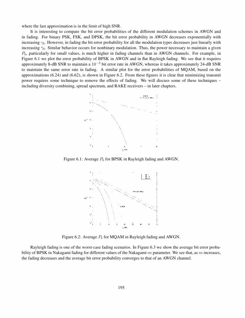
where the last approximation is in the limit of high SNR.

It is interesting to compare the bit error probabilities of the different modulation schemes in AWGN and

in fading. For binary PSK, FSK, and DPSK, the bit error probability in AWGN decreases exponentially with

increasing γb. However, in fading the bit error probability for all the modulation types decreases just linearly with

increasing γb. Similar behavior occurs for nonbinary modulation. Thus, the power necessary to maintain a given

Pb, particularly for small values, is much higher in fading channels than in AWGN channels. For example, in

Figure 6.1 we plot the error probability of BPSK in AWGN and in flat Rayleigh fading. We see that it requires

approximately 8-dB SNR to maintain a 10−3 bit error rate in AWGN, whereas it takes approximately 24-dB SNR

to maintain the same error rate in fading. A similar plot for the error probabilities of MQAM, based on the

approximations (6.24) and (6.62), is shown in Figure 6.2. From these figures it is clear that minimizing transmit

power requires some technique to remove the effects of fading. We will discuss some of these techniques –

including diversity combining, spread spectrum, and RAKE receivers – in later chapters.

Figure 6.1: Average Pb for BPSK in Rayleigh fading and AWGN.

Figure 6.2: Average Pb for MQAM in Rayleigh fading and AWGN.

Rayleigh fading is one of the worst-case fading scenarios. In Figure 6.3 we show the average bit error proba-

bility of BPSK in Nakagami fading for different values of the Nakagami-m parameter. We see that, as m increases,

the fading decreases and the average bit error probability converges to that of an AWGN channel.

195

Figure 6.3: Average Pb for BPSK in Nakagami fading.

6.3.3 Moment Generating Function Approach to Average Error Probability

The moment generating function (MGF) is a useful tool for performance analysis of modulation in fading both with

and without diversity. In this section we discuss how it can be used to simplify performance analysis of average

probability of symbol error in fading. In the next chapter we will see that it also greatly simplifies analysis in

fading channels with diversity.

The MGF for a nonnegative random variable γ with distribution pγ(γ), γ ≥ 0, is defined as

Mγ(s) =

∫ ∞

0pγ(γ)esγ dγ. (6.63)

Note that this function is just the Laplace transform of the distribution pγ(γ) with the argument reversed in sign:

L[pγ(γ)] = Mγ(−s). Thus, the MGF for most fading distributions of interest can be computed either in closed-

form using classical Laplace transforms or through numerical integration. In particular, the MGF for common

multipath fading distributions are as follows [9, Chap. 5.1].

� Rayleigh:

Mγs(s) = (1− sγs)−1. (6.64)

� Rician with factor K:

Mγs(s) =1 +K

1 +K − sγsexp

[

Ksγs1 +K − sγs

]

. (6.65)

� Nakagami-m:

Mγs(s) =(

1 − sγsm

)−m

. (6.66)

As indicated by its name, the moments E[γn] of γ can be obtained from Mγ(s) as

E[γn] =∂n

∂sn[Mγs(s)]|s=0. (6.67)

196

The basic premise of the MGF approach for computing average error probability in fading is to express the

probability of error Ps in AWGN for the modulation of interest either as an exponential function of γs,

Ps = a exp[bγs] (6.68)

for constants a and b, or as a finite-range integral of such an exponential function:

Ps =

∫ B

A

a exp[−b(x)γs] dx, (6.69)

where the constant b(x) may depend on the integrand but the SNR γs does not (and is not in the limits of integration,

either). These forms allow the average probability of error to be expressed in terms of the MGF for the fading

distribution. Specifically, if Ps = a exp[bγs], then

Ps =

∫ ∞

0

a exp[−bγ]pγs(γ)dγ = aMγs(−b). (6.70)

Since DPSK is in this form with a = 1/2 and b = 1, we see that the average probability of bit error for DPSK in

any type of fading is

Pb = 12Mγs(−1), (6.71)

where Mγs(s) is the MGF of the fading distribution. For example, using Mγs(s) for Rayleigh fading given by

(6.64) with s = −1 yields Pb = [2(1 + γb)]−1, which is the same as we obtained in (6.61). If Ps is in the integral

form of (6.69) then

Ps =

∫ ∞

0

∫ B

A

a exp[−b(x)γ]dx pγs(γ) dγ

= a

∫ B

A

[∫ ∞

0exp[−b(x)γ]pγs(γ)dγ

]

dx

= a

∫ B

AMγs(−b(x)) dx. (6.72)

In this latter case, the average probability of symbol error is a single finite-range integral of the MGF of the fading

distribution, which typically can be found in closed form or easily evaluated numerically.

Let us now apply the MGF approach to specific modulations and fading distributions. In (6.33) we gave a

general expression for Ps of coherent modulation in AWGN in terms of the Gaussian Q-function. We now make a

slight change of notation in (6.33), setting α = αM and g = .5βM to obtain

Ps(γs) = αQ(√

2gγs), (6.73)

where α and g are constants that depend on the modulation. The notation change is to obtain the error probability

as an exact MGF, as we now show.

Using the alternate Q-function representation (6.44), we get that

Ps =α

π

∫ π/2

0exp

[ −gγsin2 φ

]

dφ, (6.74)

197

which is in the desired form (6.69). Thus, the average error probability in fading for modulations with Ps =αQ(

√2gγs) in AWGN is given by

Ps =α

π

∫ ∞

0

∫ π/2

0exp

[ −gγsin2 φ

]

dφ pγs(γ) dγ

=α

π

∫ π/2

0

[∫ ∞

0

exp

[ −gγsin2 φ

]

pγs(γ)dγ

]

dφ

=α

π

∫ π/2

0Mγs

( −gsin2 φ

)

dφ, (6.75)

where Mγs(s) is the MGF associated with the distribution pγs(γ) as defined by (6.63). Recall that Table 6.1

approximates the error probability in AWGN for many modulations of interest as Ps ≈ αQ(√

2gγs), so (6.75)

gives an approximation for the average error probability of these modulations in fading. Moreover, the exact

average probability of symbol error for coherent MPSK can be obtained in a form similar to (6.75) by noting that

Craig’s formula for Ps of MPSK in AWGN given by (6.46) is in the desired form (6.69). Thus, the exact average

probability of error for MPSK becomes

Ps =

∫ ∞

0

1

π

∫ (M−1)π/M

0exp

[−gγssin2 φ

]

dφ pγs(γ) dγ

=1

π

∫ (M−1)π/M

0

[∫ ∞

0

exp

[−gγssin2 φ

]

pγs(γ) dγ

]

dφ

=1

π

∫ (M−1)π/M

0Mγs

(

− g

sin2 φ

)

dφ, (6.76)

where g = sin2(π/M) depends on the size of the MPSK constellation. The MGF Mγs(s) for Rayleigh, Rician,

and Nakagami-m distributions were given by (6.64), (6.65), and (6.66), respectively. Substituting s = −g/ sin2 φin these expressions yields the following equations.

� Rayleigh:

Mγs

(

− g

sin2 φ

)

=

(

1 +gγs

sin2 φ

)−1

. (6.77)

� Rician with factor K:

Mγs

(

− g

sin2 φ

)

=(1 +K) sin2 φ

(1 +K) sin2 φ+ gγsexp

[

− Kgγs

(1 +K) sin2 φ+ gγs

]

. (6.78)

� Nakagami-m:

Mγs

(

− g

sin2 φ

)

=

(

1 +gγs

m sin2 φ

)−m

. (6.79)

All of these functions are simple trigonometrics and are therefore easy to integrate over the finite range in (6.75)

or (6.76).

198

Example 6.31: Use the MGF technique to find an expression for the average probability of error for BPSK modu-

lation in Nakagami fading.

Solution: We use the fact that BPSK for an AWGN channel has Pb = Q(√

2γb), so α = 1 and g = 1 in (6.73).

The moment generating function for Nakagami-m fading is given by (6.79), and substituting this into (6.75) with

α = g = 1 yields

Pb =1

π

∫ π/2

0

(

1 +γb

m sin2 φ

)−m

dφ.

From (6.23) we see that the exact probability of symbol error for MQAM in AWGN contains both the Q-

function and its square. Fortunately, an alternate form of Q2(z) allows us to apply the same techniques used here

for MPSK to MQAM modulation. Specifically, an alternate representation of Q2(z) is derived in [15] as

Q2(z) =1

π

∫ π/4

0exp

[ −z2

2 sin2 φ

]

dφ. (6.80)

Note that this is identical to the alternate representation for Q(z) given in (6.44) except that the upper limit of the

integral is π/4 instead of π/2. Thus we can write (6.23) in terms of the alternate representations for Q(z) and

Q2(z) as

Ps(γs) =4

π

(

1− 1√M

)∫ π/2

0exp

(

− gγs

sin2 φ

)

dφ

− 4

π

(

1 − 1√M

)2 ∫ π/4

0exp

[

− gγs

sin2 φ

]

dφ, (6.81)

where g = 1.5/(M − 1) is a function of the MQAM constellation size. Then the average probability of symbol

error in fading becomes

Ps =

∫ ∞

0Ps(γ)pγs(γ)dγ

=4

π

(

1− 1√M

)∫ π/2

0

∫ ∞

0exp

[

− gγ

sin2 φ

]

pγs(γ) dγ dφ

− 4

π

(

1 − 1√M

)2 ∫ π/4

0

∫ ∞

0exp

[

− gγ

sin2 φ

]

pγs(γ) dγ dφ

=4

π

(

1− 1√M

)∫ π/2

0

Mγs

(

− g

sin2 φ

)

dφ

− 4

π

(

1 − 1√M

)2 ∫ π/4

0

Mγs

(

− g

sin2 φ

)

dφ. (6.82)

Thus, the exact average probability of symbol error is obtained via two finite-range integrals of the MGF over the

fading distribution, which typically can be found in closed form or easily evaluated numerically.

The MGF approach can also be applied to noncoherent and differential modulations. For example, consider

noncoherent MFSK, with Ps in AWGN given by (6.32), which is a finite sum of the desired form (6.68). Thus, in

fading, the average symbol error probability of noncoherent MFSK is given by

199

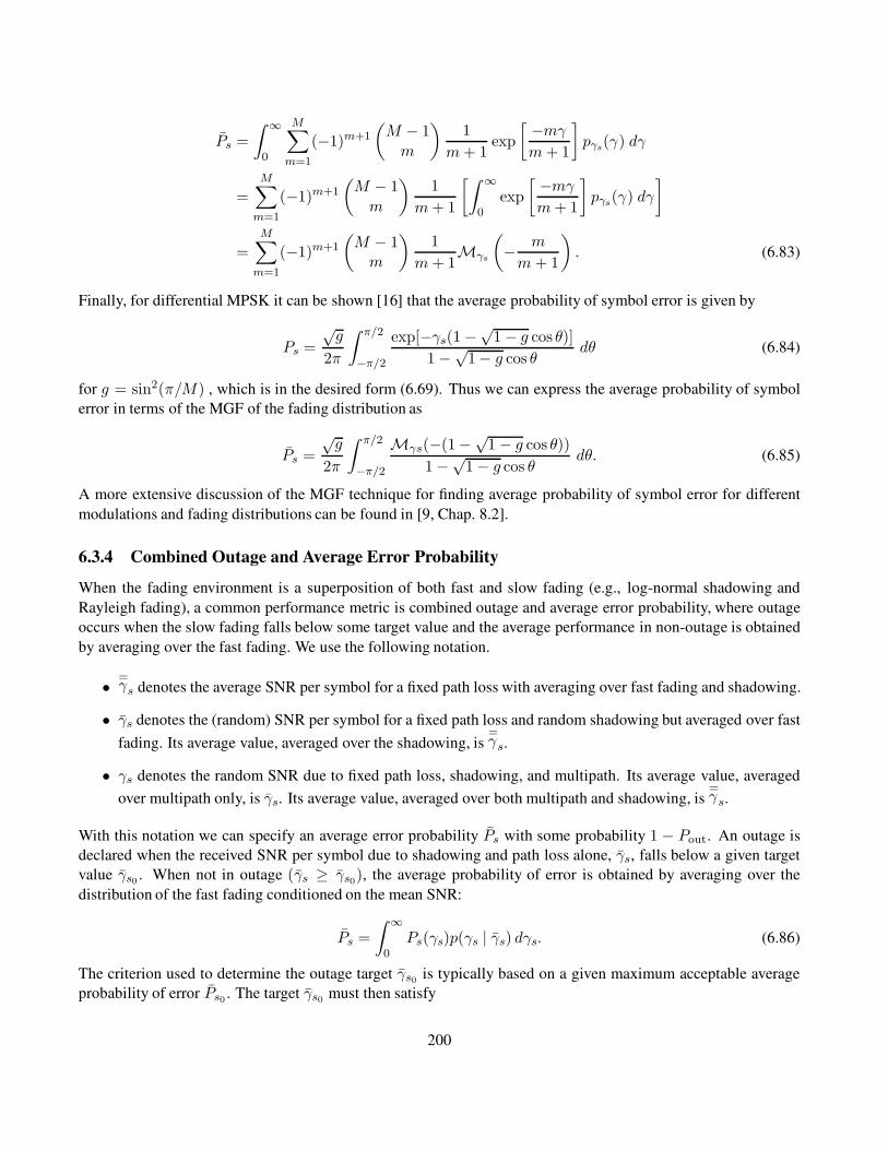
Ps =

∫ ∞

0

M∑

m=1

(−1)m+1

(

M − 1

m

)

1

m+ 1exp

[ −mγm+ 1

]

pγs(γ) dγ

=

M∑

m=1

(−1)m+1

(

M − 1

m

)

1

m+ 1

[∫ ∞

0exp

[ −mγm+ 1

]

pγs(γ) dγ

]

=

M∑

m=1

(−1)m+1

(

M − 1m

)

1

m+ 1Mγs

(

− m

m + 1

)

. (6.83)

Finally, for differential MPSK it can be shown [16] that the average probability of symbol error is given by

Ps =

√g

2π

∫ π/2

−π/2

exp[−γs(1 −√1 − g cos θ)]

1 −√1− g cos θ

dθ (6.84)

for g = sin2(π/M) , which is in the desired form (6.69). Thus we can express the average probability of symbol

error in terms of the MGF of the fading distribution as

Ps =

√g

2π

∫ π/2

−π/2

Mγs(−(1−√1 − g cos θ))

1 −√1 − g cos θ

dθ. (6.85)

A more extensive discussion of the MGF technique for finding average probability of symbol error for different

modulations and fading distributions can be found in [9, Chap. 8.2].

6.3.4 Combined Outage and Average Error Probability

When the fading environment is a superposition of both fast and slow fading (e.g., log-normal shadowing and

Rayleigh fading), a common performance metric is combined outage and average error probability, where outage

occurs when the slow fading falls below some target value and the average performance in non-outage is obtained

by averaging over the fast fading. We use the following notation.

• =γs denotes the average SNR per symbol for a fixed path loss with averaging over fast fading and shadowing.

• γs denotes the (random) SNR per symbol for a fixed path loss and random shadowing but averaged over fast

fading. Its average value, averaged over the shadowing, is=γs.

• γs denotes the random SNR due to fixed path loss, shadowing, and multipath. Its average value, averaged

over multipath only, is γs. Its average value, averaged over both multipath and shadowing, is=γs.

With this notation we can specify an average error probability Ps with some probability 1 − Pout. An outage is

declared when the received SNR per symbol due to shadowing and path loss alone, γs, falls below a given target

value γs0 . When not in outage (γs ≥ γs0), the average probability of error is obtained by averaging over the

distribution of the fast fading conditioned on the mean SNR:

Ps =

∫ ∞

0Ps(γs)p(γs | γs) dγs. (6.86)

The criterion used to determine the outage target γs0 is typically based on a given maximum acceptable average

probability of error Ps0 . The target γs0 must then satisfy

200

Ps0 =

∫ ∞

0Ps(γs)p(γs | γs0) dγs. (6.87)

It is clear that, whenever γs > γs0 , the average error probability Ps will be below the target maximum value Ps0 .

Example 6.32: Consider BPSK modulation in a channel with both log-normal shadowing (σψdB= 8 dB) and

Rayleigh fading. The desired maximum average error probability is Pb0 = 10−4, which requires γb0 = 34 dB.

Determine the value of=γb that will ensure Pb ≤ 10−4 with probability 1− Pout = .95.

Solution: We must find=γb, the average of γb in both the fast and slow fading, such that p(γb > γb0) = 1 − Pout.

For log-normal shadowing we compute this as

p(γb > 34) = p

(

γb − ¯γbσψdB

≥ 34− ¯γbσψdB

)

= Q

(

34 − ¯γbσψdB

)

= 1 − Pout, (6.88)

since, assuming units in dB, (γb − ¯γb)/σψdBis a Gauss-distributed random variable with mean 0 and standard

deviation 1. Thus, the value of ¯γb is obtained by substituting the values of Pout and σψdBin (6.88) and using a

table of Q-functions or an inversion program, which yields (34− ¯γb)/8 = −1.6 or ¯γb = 46.8 dB.

6.4 Doppler Spread

One consequence of Doppler spread is an irreducible error floor for modulation techniques using differential de-

tection. This is due to the fact that in differential modulation the signal phase associated with one symbol is used

as a phase reference for the next symbol. If the channel phase decorrelates over a symbol, then the phase refer-

ence becomes extremely noisy, leading to a high symbol error rate that is independent of received signal power.

The phase correlation between symbols and consequent degradation in performance are functions of the Doppler

frequency fD = v/λ and the symbol time Ts.

The first analysis of the irreducible error floor due to Doppler was done by Bello and Nelin in [17]. In that

work, analytical expressions for the irreducible error floor of noncoherent FSK and DPSK due to Doppler are

determined for a Gaussian Doppler power spectrum. However, these expressions are not in closed form, so they

must be evaluated numerically. Closed-form expressions for the bit error probability of DPSK in fast Rician fading

– where

Table 6.2: Correlation coefficients for different Doppler power spectra models

Type Doppler power spectrum SC(f) ρC = AC(T )/AC(0)

Rectangular P0/2BD, |f | < BD sinc(2BDT )

Gaussian (P0/√πBD)e−f

2/B2D e−(πBDT )2

Uniform scattering P0/π

√

B2D − f2, |f | < BD J0(2πBDT )

1st-order Butterworth P0BD/π(f2 +B2D) e−2πBDT

the channel decorrelates over a bit time – can be obtained using the MGF technique, with the MGF obtained based

on the general quadratic form of complex Gaussian random variables [1, Apx. B; 12, Apx. B]. A different approach

201

utilizing alternate forms of the Marcum Q-function can also be used [9, Chap. 8.2.5]. The resulting average bit

error probability for DPSK is

Pb =1

2

(

1 +K + γb(1 − ρC)

1 +K + γb

)

exp

[

− Kγb1 +K + γb

]

, (6.89)

where ρC is the channel correlation coefficient after a bit time Tb, K is the fading parameter of the Rician distribu-

tion, and γb is the average SNR per bit. For Rayleigh fading (K = 0) this simplifies to

Pb =1

2

(

1 + γb(1− ρC)

1 + γb

)

. (6.90)

Letting γb → ∞ in (6.89) yields the irreducible error floor:

Pfloor =(1 − ρC)e−K

2(DPSK). (6.91)

A similar approach is used in [18] to bound the bit error probability of DQPSK in fast Rician fading as

Pb ≤1

2

(

1−√

(ρC γs/√

2)2

(γs + 1)2 − (ρC γs/√

2)2

)

exp

[

− (2−√

2)Kγs/2

(γs + 1) − (ρC γs/√

2)

]

, (6.92)

where K is as before, ρC is the channel correlation coefficient after a symbol time Ts, and γs is the average SNR

per symbol. Letting γs → ∞ yields the irreducible error floor:

Pfloor =1

2

(

1 −√

(ρC/√

2)2

1− (ρC/√

2)2

)

exp

[

−(2 −√

2)(K/2)

1− ρC/√

2

]

(DQPSK). (6.93)

As discussed in Section 3.2.1, the channel correlation AC(τ) over time τ equals the inverse Fourier transform

of the Doppler power spectrum SC(f) as a function of Doppler frequency f . The correlation coefficient is thus

ρC = AC(T )/AC(0) evaluated at T = Ts for DQPSK or at T = Tb for DPSK. Table 6.2, from [19], gives the

value of ρC for several different Doppler power spectra models, where BD is the Doppler spread of the channel.

Assuming the uniform scattering model (ρC = J0(2πfDTb)) and Rayleigh fading (K = 0) in (6.91) yields an

irreducible error for DPSK of

Figure 6.4: Average Pb for DPSK in fast Rician fading with uniform scattering.

P floor =1 − J0(2πfDTb)

2≈ .5(πfDTb)

2, (6.94)

202

where BD = fD = v/λ is the maximum Doppler in the channel. Note that in this expression the error floor

decreases with data rate R = 1/Tb. This is true in general for irreducible error floors of differential modulation

due to Doppler, since the channel has less time to decorrelate between transmitted symbols. This phenomenon is

one of the few instances in digital communications where performance improves as data rate increases.

A plot of (6.89), the error probability of DPSK in fast Rician fading, for uniform scattering (ρC = J0(2πfDTb))

and different values of fDTb is shown in Figure 6.4. We see from this figure that the error floor starts to dominate

at γb = 15 dB in Rayleigh fading (K = 0), and as K increases the value of γb where the error floor dominates

also increases. We also see that increasing the data rate Rb = 1/Tb by an order of magnitude decreases the error

floor by roughly two orders of magnitude.

Example 6.33: Assume a Rayleigh fading channel with uniform scattering and a maximum Doppler of fD = 80

Hz. For what approximate range of data rates will the irreducible error floor of DPSK be below 10−4?

Solution: We have P floor ≈ .5(πfDTb)2 < 10−4. Solving for Tb with fD = 80 Hz, we get

Tb <

√2 · 10−4

π · 80= 5.63 · 10−5,

which yields R > 17.77 kbps.

Deriving analytical expressions for the irreducible error floor becomes intractable with more complex modulations,

in which case simulations are often used. In particular, simulations of the irreducible error floor for π/4-DQPSK

with square-root raised cosine filtering have been conducted (since this modulation is used in the IS-136 TDMA

standard) in [20, 21]. These simulation results indicate error floors between 10−3 and 10−4. As expected, in

these simulations the error floor increases with vehicle speed, since at higher vehicle speeds the channel typically

decorrelates more over a given symbol time.

6.5 Intersymbol Interference

Frequency-selective fading gives rise to intersymbol interference, where the received symbol over a given symbol

period experiences interference from other symbols that have been delayed by multipath. Since increasing signal

power also increases the power of the ISI, this interference gives rise to an irreducible error floor that is independent

of signal power. The irreducible error floor is difficult to analyze because it depends on the modulation format and

the ISI characteristics, which in tum depend on the characteristics of the channel and the sequence of transmitted

symbols.

The first extensive analysis of the degradation in symbol error probability due to ISI was done by Bello and

Nelin [22]. In that work, analytical expressions for the irreducible error floor of coherent FSK and noncoherent

DPSK are determined assuming a Gaussian delay profile for the channel. To simplify the analysis, only ISI asso-

ciated with adjacent symbols was taken into account. Even with this simplification, the expressions are complex

and must be approximated for evaluation. A more accurate analytical analysis can be found in [23, Chap. 8.2],

where the irreducible error floor is evaluated based on both the worst-case sequence of transmitted symbols and by

averaging over all possible symbol sequences. These expressions are also complex to evaluate owing to their de-

pendence on the channel and symbol sequence characteristics. A simple approximation to symbol error probability

with ISI can be obtained by treating the ISI as uncorrelated white Gaussian noise. Then the SNR becomes

γs =Pr

N0B + I, (6.95)

203

Figure 6.5: lrreducible error versus normalized rms delay spread for Gaussian power delay profile. (Reprinted by

permission from [?, Fig. 9], c© 1987 IEEE.)

where Pr is the received power associated with the line-of-sight signal component, and I is the received power

associated with the ISI. In a static channel the resulting probability of symbol error will be Ps(γs), where Ps is

the probability of symbol error in AWGN. If both the LOS signal component and the ISI experience flat fading,

then γs will be a random variable with distribution p(γs), and the average symbol error probability is then P s =∫

Ps(γs)p(γs) dγs. Note that γs is the ratio of two random variables – the LOS received power Pr and the ISI

received power I – and thus the resulting distribution p(γs) may be hard to obtain and typically is not in closed

form.

Irreducible error floors due to ISI are often obtained by simulation, which can easily incorporate different

channel models, modulation formats, and symbol sequence characteristics [?, 20, 21, 25, 26, 27, ?]. The earliest

of these works is [?]. The extensive simulations in this work determined the irreducible error floor due to ISI for

BPSK, DPSK, QPSK, OQPSK and MSK modulations with different pulse shapes and for channels with differ-

ent power delay profiles, including a Gaussian, exponential, equal-amplitude two-ray, and empirical power delay

profile. The results of [?] indicate that the irreducible error floor is more sensitive to the rms delay spread of the

channel than to the shape of its power delay profile. Moreover, pulse shaping can significantly impact the error

floor: for the raised cosine pulses discussed in Section 5.5, increasing β from 0 to 1 can reduce the error floor by

over an order of magnitude.

The simulation results of [?] are shown in Figure 6.5. This figure plots the irreducible bit error rate as a

function of normalized rms delay spread d = σTm/Ts for BPSK, QPSK, OQPSK, and MSK modulation assuming

a static channel with a Gaussian power delay profile. We see from the figure that, for all modulations, we can

approximately bound the irreducible error floor as

Pfloor ≤ K

(

σTm

Ts

)2

(6.96)

for K a constant that depends on the modulation type, the transmit and receive filtering, and the power delay

profile. For the modulation types in Figure 6.5 we see thatK ranges from about 0.4 for MSK to 1 for BPSK. Other

simulation results [?, 25, 26] support this bound as well. This bound can also be derived analytically based on

group delay. Details can be found in [29, Chapter 12.3.2].

204

This bound imposes severe constraints on data rate even when symbol error probabilities on the order of

10−2 are acceptable, and usually this is a very high error probability even with strong error correction codes. For

example, the rms delay spread in a typical urban environment is approximately σTm = 2.5 µs. To keep σTm < .1Tsrequires that the data rate not exceed 40 kbaud, which generally isn’t enough for high-speed data applications. In

rural environments, where multipath is not attenuated to the same degree as in cities, σTm ≈ 25 µs, which reduces

the maximum data rate to 4 kbaud.

Example 6.34: Using the approximation P floor ≤ K(σTm/Ts)2 of (6.96) with K = 0.4 for BPSK and K = 0.7,

find the maximum data rate that can be transmitted through a channel with delay spread σTm = 3 µs, using either

BPSK or QPSK modulation, such that the probability of bit error Pb is less than 10−3.

Solution: For BPSK, we set P floor = .4(σTm/Tb)2 and so require Tb ≥ σTm/

√

Pfloor/.4 = 94.87 µs, which leads

to a data rate of R = 1/Tb = 15 kbps. For QPSK, we have Ts ≥ σTm/√

Pfloor/.7 = 113.39 µs. Since there are

two bits per symbol, this leads to a data rate of R = 2/Ts = 17.64 kbps. This indicates that, for a given data rate,

QPSK is more robust to ISI than BPSK because its symbol time is slower, even though the K value in the error

floor bound (6.96) is higher for the larger constellation size of QPSK versus BPSK. In general K increases in the

bound of (6.96) as the constellation size increases, but large constellations are still more robust to ISI than smaller

ones due to their longer symbol times.

205

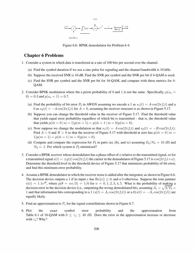
Figure 6.6: BPSK demodulator for Problem 6-4.

Chapter 6 Problems

1. Consider a system in which data is transferred at a rate of 100 bits per second over the channel.

(a) Find the symbol duration if we use a sinc pulse for signaling and the channel bandwidth is 10 kHz.

(b) Suppose the received SNR is 10 dB. Find the SNR per symbol and the SNR per bit if 4-QAM is used.

(c) Find the SNR per symbol and the SNR per bit for 16-QAM, and compare with these metrics for 4-

QAM.

2. Consider BPSK modulation where the a priori probability of 0 and 1 is not the same. Specifically, p(sn =

0) = 0.3 and p(sn = 1) = 0.7.

(a) Find the probability of bit error Pb in AWGN assuming we encode a 1 as s1(t) = A cos(2πfct) and a

0 as s2(t) = −A cos(2πfct) for A > 0, assuming the receiver structure is as shown in Figure 5.17.

(b) Suppose you can change the threshold value in the receiver of Figure 5.17. Find the threshold value

that yields equal error probability regardless of which bit is transmitted – that is, the threshold value

that yields p(m = 0 |m = 1)p(m = 1) = p(m = 1 |m = 0)p(m = 0).

(c) Now suppose we change the modulation so that s1(t) = A cos(2πfct) and s2(t) = −B cos(2πfct).

Find A > 0 and B > 0 so that the receiver of Figure 5.17 with threshold at zero has p(m = 0 |m =

1)p(m = 1) = p(m = 1 |m = 0)p(m = 0).

(d) Compute and compare the expression for Pb in parts (a), (b), and (c) assuming Eb/N0 = 10 dB and

N0 = .1. For which system is Pb minimized?

3. Consider a BPSK receiver whose demodulator has a phase offset of φ relative to the transmitted signal, so for

a transmitted signal s(t) = ±g(t) cos(2πfct) the carrier in the demodulator of Figure 5.17 is cos(2πfct+φ).

Determine the threshold level in the threshold device of Figure 5.17 that minimizes probability of bit error,

and find this minimum error probability.

4. Assume a BPSK demodulator in which the receiver noise is added after the integrator, as shown in Figure 6.6.

The decision device outputs a 1 if its input x has Re{x} ≥ 0, and a 0 otherwise. Suppose the tone jammer

n(t) = 1.1ejθ, where p(θ = nπ/3) = 1/6 for n = 0, 1, 2, 3, 4, 5. What is the probability of making a

decision error in the decision device (i.e., outputting the wrong demodulated bit), assumingAc =√

2/Tb =1 and that information bits corresponding to a 1 (s(t) = Ac cos(2πfct)) or a 0(s(t) = −Ac cos(2πfct)) are

equally likely.

5. Find an approximation to Ps for the signal constellations shown in Figure 6.7.

6. Plot the exact symbol error probability and the approximation from

Table 6.1 of 16-QAM with 0 ≤ γs ≤ 30 dB. Does the error in the approximation increase or decrease

with γs? Why?

206

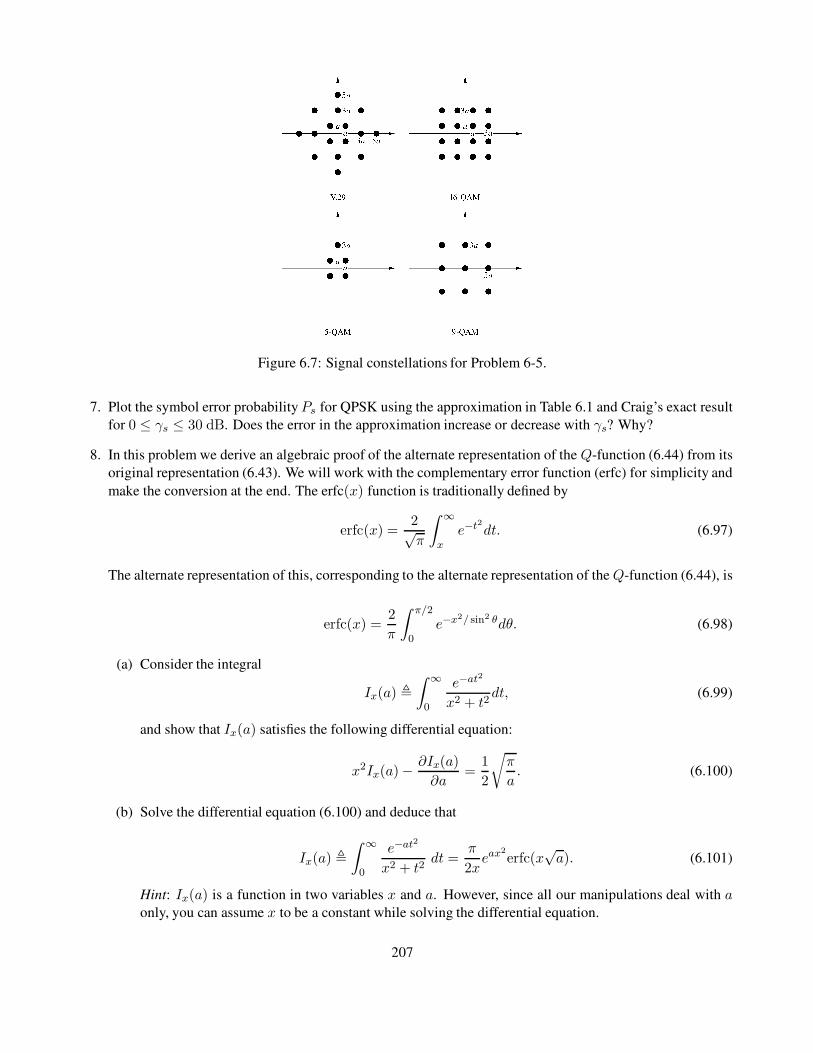
Figure 6.7: Signal constellations for Problem 6-5.

7. Plot the symbol error probabilityPs for QPSK using the approximation in Table 6.1 and Craig’s exact result

for 0 ≤ γs ≤ 30 dB. Does the error in the approximation increase or decrease with γs? Why?

8. In this problem we derive an algebraic proof of the alternate representation of the Q-function (6.44) from its

original representation (6.43). We will work with the complementary error function (erfc) for simplicity and

make the conversion at the end. The erfc(x) function is traditionally defined by

erfc(x) =2√π

∫ ∞

x

e−t2dt. (6.97)

The alternate representation of this, corresponding to the alternate representation of theQ-function (6.44), is

erfc(x) =2

π

∫ π/2

0

e−x2/ sin2 θdθ. (6.98)

(a) Consider the integral

Ix(a) ,

∫ ∞

0

e−at2

x2 + t2dt, (6.99)

and show that Ix(a) satisfies the following differential equation:

x2Ix(a)−∂Ix(a)

∂a=

1

2

√

π

a. (6.100)

(b) Solve the differential equation (6.100) and deduce that

Ix(a) ,

∫ ∞

0

e−at2

x2 + t2dt =

π

2xeax

2erfc(x

√a). (6.101)

Hint: Ix(a) is a function in two variables x and a. However, since all our manipulations deal with aonly, you can assume x to be a constant while solving the differential equation.

207

(c) Setting a = 1 in (6.101) and making a suitable change of variables in the left-hand side of (6.101),

derive the alternate representation of the erfc function:

erfc(x) =2

π

∫ π/2

0e−x

2/ sin2 θdθ.

(d) Convert this alternate representation of the erfc function to the alternate representation of the Q-

function.

9. Consider a communication system that uses BPSK signaling, with average signal power of 100 W and noise

power at the receiver of 4 W. Based on its error probability, can this system be used for transmission of data?

Can it be used for voice? Now consider the presence of fading with an average SNR γb = 20 dB. How do

your answers to the previous questions change?

10. Consider a cellular system at 900 MHz with a transmission rate of 64 kbps and multipath fading. Explain

which performance metric – average probability of error or outage probability – is more appropriate (and

why) for user speeds of l mph, 10 mph, and 100 mph.

11. Derive the expression for the moment generating function for SNR in Rayleigh fading.

12. This problem illustrates why satellite systems that must compensate for shadow fading are going bankrupt.

Consider an LEO satellite system orbiting 500 km above the earth. Assume that the signal follows a free-

space path-loss model with no multipath fading or shadowing. The transmitted signal has a carrier frequency

of 900 MHz and a bandwidth of 10 kHz. The handheld receivers have noise power spectral density of 10−16

mW/Hz (total noise power is N0B). Assume nondirectional antennas (0-dB gain) at both the transmitter and

receiver. Suppose the satellite must support users in a circular cell on the earth of radius 100 km at a BER

of 10−6.

(a) For DPSK modulation, find the transmit power needed for all users in the cell to meet the 10−6 BER

target.

(b) Repeat part (a) assuming that the channel also experiences log-normal shadowing with σψdB= 8 dB

and that users in a cell must have Pb = 10−6 (for each bit) with probability 0.9.

13. In this problem we explore the power penalty involved in going from BPSK to the higher-level signal mod-

ulation of 16-PSK.

(a) Find the minimum distance between constellation points in 16-PSK modulation as a function of signal

energy Es.

(b) Find αM and βM such that the symbol error probability of 16-PSK in AWGN is approximately

Ps ≈ αMQ(√

βMγs).

(c) Using your expression in part (b), find an approximation for the average symbol error probability of

16-PSK in Rayleigh fading in terms of γs.

(d) Convert the expressions for average symbol error probability of 16-PSK in Rayleigh fading to an ex-

pression for average bit error probability, assuming Gray coding.

(e) Find the approximate value of γb required to obtain a BER of 10−3 in Rayleigh fading for BPSK and

16-PSK. What is the power penalty in going to the higher-level signal constellation at this BER?

208

14. Find a closed-form expression for the average probability of error for DPSK modulation in Nakagami-mfading. Evalute for m = 4 and γb = 10 dB.

15. The Nakagami distribution is parameterized by m, which ranges from m = .5 to m = ∞. Them-parameter

measures the ratio of LOS signal power to multipath power, so m = 1 corresponds to Rayleigh fading,

m = ∞ corresponds to an AWGN channel with no fading, and m = .5 corresponds to fading that results in

performance that is worse than with a Rayleigh distribution. In this problem we explore the impact of the

parameter m on the performance of BPSK modulation in Nakagami fading.

Plot the average bit error P b of BPSK modulation in Nakagami fading with average SNR ranging from 0 dB

to 20 dB for m parameters m = 1 (Rayleigh), m = 2, and m = 4. (The moment generating function

technique of Section 6.3.3 should be used to obtain the average error probability.) At an average SNR of

10 dB, what is the difference in average BER?

16. Assume a cellular system with log-normal shadowing plus Rayleigh fading. The signal modulation is DPSK.

The service provider has determined that it can deal with an outage probability of .01 – that is, 1 in 100

customers can be unhappy at any given time. In nonoutage, the voice BER requirement is P b = 10−3.

Assume a noise PSD N0/2 with N0 = 10−16 mW/Hz, a signal bandwidth of 30 kHz, a carrier frequency of

900 MHz, free-space path-loss propagation with nondirectional antennas, and a shadowing standard devia-

tion of σψdB= 6 dB. Find the maximum cell size that can achieve this performance if the transmit power at

the mobiles is limited to 100 mW.

17. Consider a cellular system with circular cells of radius 100 meters. Assume that propagation follows the

simplified path-loss model with K = 1, d0 = 1 m, and γ = 3. Assume the signal experiences (in addition

to path loss) log-normal shadowing with σψdB= 4 as well as Rayleigh fading. The transmit power at

the base station is Pt = 100 mW, the system bandwidth is B = 30 kHz, and the noise PSD N0/2 has

N0 = 10−14W/Hz. Assuming BPSK modulation, we want to find the cell coverage area (percentage of

locations in the cell) where users have average Pb of less than 10−4.

(a) Find the received power due to path loss at the cell boundary.

(b) Find the minimum average received power (due to path loss and shadowing) such that, with Rayleigh

fading about this average, a BPSK modulated signal with this average received power at a given cell

location has P b < 10−4.

(c) Given the propagation model for this system (simplified path loss, shadowing, and Rayleigh fading),

find the percentage of locations in the cell where P b < 10−4 under BPSK modulation.

18. In this problem we derive the probability of bit error for DPSK in fast Rayleigh fading. By symmetry, the

probability of error is the same for transmitting a 0-bit or a 1-bit. Let us assume that over time kTb a 0-bit is

transmitted, so the transmitted symbol at time kTb is the same as at time k−1: s(k) = s(k−1). In fast fading,

the corresponding received symbols are r(k−1) = gk−1s(k−1)+n(k−1) and r(k) = gks(k−1)+n(k),

where gk−1 and gk are the fading channel gains associated with transmissions over times (k−1)Tb and kTb.

(a) Show that the decision variable that is input to the phase comparator of Figure 5.20 in order to extract

the phase difference is r(k)r∗(k − 1) = gkg∗k−1 + gks(k− 1)∗nk−1 + g∗k−1s

∗k−1nk + nkn

∗k−1.

Assuming a reasonable SNR, the last term nkn∗k−1 of this expression can be neglected. So neglecting

this term and then defining nk = s∗k−1nk and nk−1 = s∗k−1nk−1, we get a new random variable

z = gkg∗k−1 + gkn

∗k−1 + g∗k−1nk. Given that a 0-bit was transmitted over time kTb, an error is made

209

if x = Re{z} < 0, so we must determine the distribution of x. The characteristic function for x is the

two-sided Laplace transform of the distribution of x:

ΦX(s) =

∫ ∞

−∞pX(s)e−sx dx = E[e−sx].

This function will have a left-plane pole p1 and a right-plane pole p2, so it can be written as

ΦX(s) =p1p2

(s− p1)(s− p2).

The left-plane pole p1 corresponds to the distribution pX(x) for x ≥ 0, and the rightplane pole corre-

sponds to the distribution pX(x) for x < 0.

(b) Show through partial fraction expansion that ΦX(s) can be written as

ΦX(s) =p1p2

p1 − p2

1

s − p1+

p1p2

p2 − p1

1

s− p2.

An error is made if x = Re{z} < 0, so here we need only consider the distribution pX(x) for x < 0

corresponding to the second term of ΦX(s).

(c) Show that the inverse Laplace transform of the second term of ΦX(s) from part (b) is

pX(x) =p1p2

p2 − p1ep2X , x < 0.

(d) Use part (c) to show that Pb = −p1/(p2 − p1).

In x = Re{z} = Re{gkg∗k−1 + gkn∗k−1 + g∗k−1nk}, the channel gains gk, gk−1 and noises nk, nk−1

are complex Gaussian random variables. Thus, the poles p1, p2 in pX(x) are derived using the general

quadratic form of complex Gaussian random variables [1, Apx. B; 12, Apx. B] as

p1 =−1

N0(γb[1 + ρc] + 1)and p2 =

1

N0(γb[1 − ρc] + 1)

for ρC the correlation coefficient of the channel over the bit time Tb.

(e) Find a general expression for Pb in fast Rayleigh fading using these values of p1 and p2 in the Pbexpression from part (d).

(f) Show that this reduces to the average probability of error P b = 1/2(1+γb) for a slowly fading channel

that does not decorrelate over a bit time.

19. Plot the bit error probability for DPSK in fast Rayleigh fading for γb ranging from 0 dB to 60 dB and

ρC = J0(2πBDT ) with BDT = .01, .001, and .0001. For each value of BDT , at approximately what value

of γb does the error floor dominate the error probability?

20. Find the irreducible error floor due to Doppler for DQPSK modulation with a data rate of 40 kbps, assuming

a Gaussian Doppler power spectrum with BD = 80 Hz and Rician fading with K = 2.

21. Consider a wireless channel with an average delay spread of 100 ns and a Doppler spread of 80 Hz. Given

the error floors due to Doppler and ISI – and assuming DQPSK modulation in Rayleigh fading and uniform

scattering – approximately what range of data rates can be transmitted over this channel with a BER of less

than 10−4?

210

22. Using the error floors of Figure 6.5, find the maximum data rate that can be transmitted through a channel

with delay spread σTm = 3 µs (using BPSK, QPSK, or MSK modulation) such that the probability of bit

error Pb is less than 10−3.

211

Bibliography

[1] J. G. Proakis and M. Salehi, Digital Communications, 5th ed., McGraw-Hill, New York, 2008.

[2] M. K. Simon, S. M. Hinedi, and W. C. Lindsey, Digital Communication Techniques: Signal Design and

Detection, Prentice-Hall, Englewood Cliffs, NJ, 1995.

[3] S. Rhodes, “Effect of noisy phase reference on coherent detection of offset-QPSK signals,” IEEE Trans.

Commun., pp. 1046–55, August 1974.

[4] N. R. Sollenberger and J. C.-I. Chuang, “Low-overhead symbol timing and carrier recovery for portable

TDMA radio systems,” IEEE Trans. Commun., pp. 1886–92, October 1990.

[5] R. Pawula, S. Rice, and J. Roberts, “Distribution of the phase angle between two vectors perturbed by Gaus-

sian noise,” IEEE Trans. Commun., pp. 1828–41, August 1982.

[6] W. Cowley and L. Sabel, “The performance of two symbol timing recovery algorithms for PSK demodula-

tors,” IEEE Trans. Commun., pp. 2345–55, June 1994.

[7] W. T. Webb and L. Hanzo, Modern Quadrature Amplitude Modulation, IEEE/Pentech Press, London, 1994.

[8] X. Tang, M.-S. Alouini, and A. Goldsmith, “Effect of channel estimation error on M-QAM BER performance

in Rayleigh fading,” IEEE Trans. Commun., pp. 1856–64, December 1999.

[9] M. K. Simon and M.-S. Alouini, Digital Communication over Fading Channels: A Unified Approach to

Performance Analysis, 2nd Ed., Wiley, New York, 2004.

[10] S. Hinedi, M. Simon, and D. Raphaeli, “The performance of noncoherent orthogonal M-FSK in the presence

of timing and frequency errors,” IEEE Trans. Commun., pp. 922–33, February–April 1995.

[11] E. Grayver and B. Daneshrad, “A low-power all-digital FSK receiver for deep space applications,” IEEE

Trans. Commun., pp. 911–21, May 2001.

[12] M. Schwartz, W. R. Bennett, and S. Stein, Communication Systems and Techniques, McGraw-Hill, New York,

1966 [reprinted 1995 by Wiley/IEEE Press].

[13] J. Craig, “New, simple and exact result for calculating the probability of error for two-dimensional signal

constellations,” Proc. Military Commun. Conf., pp. 25.5.1–25.5.5, November 1991.

[14] F. S. Weinstein, “Simplified relationships for the probability distribution of the phase of a sine wave in narrow-

band normal noise,” IEEE Trans. Inform. Theory, pp. 658–61, September 1974.

[15] M. K. Simon and D. Divsalar, “Some new twists to problems involving the Gaussian probability integral,”

IEEE Trans. Commun., pp. 200–10, Febmary 1998.

212

[16] R. F. Pawula, “A new formula for MDPSK symbol error probability,” IEEE Commun. Lett., pp. 271–2, Octo-

ber 1998.

[17] P. A. Bello and B. D. Nelin, “The influence of fading spectrum on the bit error probabilities of incoherent and

differentially coherent matched filter receivers,” IEEE Trans. Commun. Syst., pp. 160–8, June 1962.

[18] P. Y. Kam, “Tight bounds on the bit-error probabilities of 2DPSK and 4DPSK in nonselective Rician fading,”

IEEE Trans. Commun., pp. 860–2, July 1998.

[19] P. Y. Kam, “Bit error probabilities of MDPSK over the nonselective Rayleigh fading channel with diversity

reception,” IEEE Trans. Commun., pp. 220–4, February 1991.

[20] V. Fung, R. S. Rappaport, and B. Thoma, “Bit error simulation for π/4 DQPSK mobile radio communication

using two-ray and measurement based impulse response models,” IEEE J. Sel. Areas Commun., pp. 393–405,

April 1993.

[21] S. Chennakeshu and G. J. Saulnier, “Differential detection of π/4-shifted-DQPSK for digital cellular radio,”

IEEE Trans. Veh. Tech., pp. 46–57, Febmary 1993.

[22] P. A. Bello and B. D. Nelin, “ The effects of frequency selective fading on the binary error probabilities

of incoherent and differentially coherent matched filter receivers,” IEEE Trans. Commun. Syst., pp. 170–86,

June 1963.

[23] M. B. Pursley, Introduction to Digital Communications, Prentice-Hall, Englewood Cliffs, NJ, 2005.

[24] J. C.-I. Chuang, “The effects of time delay spread on portable radio communications channels with digital

modulation,” IEEE J. Sel. Areas Commun., pp. 879–89, June 1987.

[25] N. R. Sollenberger, J. C. I. Chuang, L. F. Chang, S. Ariyavisitakul and H. Arnold, “Architecture and im-

plementation of an efficient and robust TDMA frame structure for digital portable communications,” IEEE

Transactions on Vehicular Technology, vol. 40, no. 1, pp. 250-260, Feb. 1991.

[26] J. C. I. Chuang, ”The effects of delay spread on 2-PSK, 4-PSK, 8-PSK and 16-QAM in a portable radio

environment,” IEEE Transactions on Vehicular Technology, vol. 38, no. 2, pp. 43-45, May 1989.

[27] C. Liu and K. Feher, “Bit error rate performance of π/4 DQPSK in a frequency selective fast Rayleigh fading

channel,” IEEE Trans. Veh. Tech., pp. 558–68, August 1991.

[28] S. Gumnathan and K. Feher, “Multipath simulation models for mobile radio channels,” Proc. IEEE Veh. Tech.

Conf., pp. 131–4, May 1992.

[29] Wireless Communications, 2nd Ed, A. F. Molisch, John Wiley and Sons, 2010.

213