andrea macchi giovanni moruzzi francesco pegoraro problems ... · of course, this book of problems...
TRANSCRIPT

Problems in Classical Electromagnetism
Andrea MacchiGiovanni MoruzziFrancesco Pegoraro
157 Exercises with Solutions

Problems in Classical Electromagnetism

Andrea Macchi • Giovanni MoruzziFrancesco Pegoraro
Problems in ClassicalElectromagnetism
157 Exercises with Solutions
123
Andrea MacchiDepartment of Physics “Enrico Fermi”University of PisaPisaItaly
Giovanni MoruzziDepartment of Physics “Enrico Fermi”University of PisaPisaItaly
Francesco PegoraroDepartment of Physics “Enrico Fermi”University of PisaPisaItaly
ISBN 978-3-319-63132-5 ISBN 978-3-319-63133-2 (eBook)DOI 10.1007/978-3-319-63133-2
Library of Congress Control Number: 2017947843
© Springer International Publishing AG 2017This work is subject to copyright. All rights are reserved by the Publisher, whether the whole or partof the material is concerned, specifically the rights of translation, reprinting, reuse of illustrations,recitation, broadcasting, reproduction on microfilms or in any other physical way, and transmissionor information storage and retrieval, electronic adaptation, computer software, or by similar or dissimilarmethodology now known or hereafter developed.The use of general descriptive names, registered names, trademarks, service marks, etc. in this
publication does not imply, even in the absence of a specific statement, that such names are exempt fromthe relevant protective laws and regulations and therefore free for general use.The publisher, the authors and the editors are safe to assume that the advice and information in thisbook are believed to be true and accurate at the date of publication. Neither the publisher nor theauthors or the editors give a warranty, express or implied, with respect to the material contained herein orfor any errors or omissions that may have been made. The publisher remains neutral with regard to
jurisdictional claims in published maps and institutional affiliations.
Printed on acid-free paper
This Springer imprint is published by Springer NatureThe registered company is Springer International Publishing AG
The registered company address is: Gewerbestrasse 11, 6330 Cham, Switzerland

Preface
This book comprises 157 problems in classical electromagnetism, originating from
the second-year course given by the authors to the undergraduate students of
physics at the University of Pisa in the years from 2002 to 2017. Our course covers
the basics of classical electromagnetism in a fairly complete way. In the first part,
we present electrostatics and magnetostatics, electric currents, and magnetic
induction, introducing the complete set of Maxwell’s equations. The second part is
devoted to the conservation properties of Maxwell’s equations, the classical theory
of radiation, the relativistic transformation of the fields, and the propagation of
electromagnetic waves in matter or along transmission lines and waveguides.
Typically, the total amount of lectures and exercise classes is about 90 and
45 hours, respectively. Most of the problems of this book were prepared for the
intermediate and final examinations. In an examination test, a student is requested
to solve two or three problems in 3 hours. The more complex problems are pre-
sented and discussed in detail during the classes.
The prerequisite for tackling these problems is having successfully passed the
first year of undergraduate studies in physics, mathematics, or engineering,
acquiring a good knowledge of elementary classical mechanics, linear algebra,
differential calculus for functions of one variable. Obviously, classical electro-
magnetism requires differential calculus involving functions of more than one
variable. This, in our undergraduate programme, is taught in parallel courses
of the second year. Typically, however, the basic concepts needed to write down the
Maxwell equations in differential form are introduced and discussed in our elec-
tromagnetism course, in the simplest possible way. Actually, while we do not
require higher mathematical methods as a prerequisite, the electromagnetism course
is probably the place where the students will encounter for the first time topics such
as Fourier series and transform, at least in a heuristic way.
In our approach to teaching, we are convinced that checking the ability to solve a
problem is the best way, or perhaps the only way, to verify the understanding of the
theory. At the same time, the problems offer examples of the application
of the theory to the real world. For this reason, we present each problem with a title
that often highlights its connection to different areas of physics or technology,
v

so that the book is also a survey of historical discoveries and applications of
classical electromagnetism. We tried in particular to pick examples from different
contexts, such as, e.g., astrophysics or geophysics, and to include topics that, for
some reason, seem not to be considered in several important textbooks, such as,
e.g., radiation pressure or homopolar/unipolar motors and generators. We also
included a few examples inspired by recent and modern research areas, including,
e.g., optical metamaterials, plasmonics, superintense lasers. These latter topics
show that nowadays, more than 150 years after Maxwell's equations, classical
electromagnetism is still a vital area, which continuously needs to be understood
and revisited in its deeper aspects. These certainly cannot be covered in detail in a
second-year course, but a selection of examples (with the removal of unnecessary
mathematical complexity) can serve as a useful introduction to them. In our
problems, the students can have a first glance at “advanced” topics such as, e.g., the
angular momentum of light, longitudinal waves and surface plasmons, the princi-
ples of laser cooling and of optomechanics, or the longstanding issue of radiation
friction. At the same time, they can find the essential notions on, e.g., how an
optical fiber works, where a plasma display gets its name from, or the principles of
funny homemade electrical motors seen on YouTube.
The organization of our book is inspired by at least two sources, the book
Selected Problems in Theoretical Physics (ETS Pisa, 1992, in Italian; World
Scientific, 1994, in English) by our former teachers and colleagues A. Di Giacomo,
G. Paffuti and P. Rossi, and the great archive of Physics Examples and other
Pedagogic Diversions by Prof. K. McDonald (http://puhep1.princeton.edu/%
7Emcdonald/examples/) which includes probably the widest source of advanced
problems and examples in classical electromagnetism. Both these collections are
aimed at graduate and postgraduate students, while our aim is to present a set of
problems and examples with valuable physical contents, but accessible at the
undergraduate level, although hopefully also a useful reference for the graduate
student as well.
Because of our scientific background, our inspirations mostly come from the
physics of condensed matter, materials and plasmas as well as from optics, atomic
physics and laser–matter interactions. It can be argued that most of these subjects
essentially require the knowledge of quantum mechanics. However, many phe-
nomena and applications can be introduced within a classical framework, at least in
a phenomenological way. In addition, since classical electromagnetism is the first
field theory met by the students, the detailed study of its properties (with particular
regard to conservation laws, symmetry relations and relativistic covariance) pro-
vides an important training for the study of wave mechanics and quantum field
theories, that the students will encounter in their further years of physics study.
In our book (and in the preparation of tests and examinations as well), we tried to
introduce as many original problems as possible, so that we believe that we have
reached a substantial degree of novelty with respect to previous textbooks.
Of course, the book also contains problems and examples which can be found in
existing literature: this is unavoidable since many classical electromagnetism
problems are, indeed, classics! In any case, the solutions constitute the most
vi Preface

important part of the book. We did our best to make the solutions as complete and
detailed as possible, taking typical questions, doubts and possible mistakes by the
students into account. When appropriate, alternative paths to the solutions are
presented. To some extent, we tried not to bypass tricky concepts and ostensible
ambiguities or “paradoxes” which, in classical electromagnetism, may appear more
often than one would expect.
The sequence of Chapters 1–12 follows the typical order in which the contents
are presented during the course, each chapter focusing on a well-defined topic.
Chapter 13 contains a set of problems where concepts from different chapters are
used, and may serve for a general review. To our knowledge, in some under-
graduate programs the second-year physics may be “lighter” than at our department,
i.e., mostly limited to the contents presented in the first six chapters of our book
(i.e., up to Maxwell's equations) plus some preliminary coverage of radiation
(Chapter 10) and wave propagation (Chapter 11). Probably this would be the choice
also for physics courses in the mathematics or engineering programs. In a physics
program, most of the contents of our Chapters 7–12 might be possibly presented in
a more advanced course at the third year, for which we believe our book can still be
an appropriate tool.
Of course, this book of problems must be accompanied by a good textbook
explaining the theory of the electromagnetic field in detail. In our course, in
addition to lecture notes (unpublished so far), we mostly recommend the volume II
of the celebrated Feynman Lectures on Physics and the volume 2 of the Berkeley
Physics Course by E. M. Purcell. For some advanced topics, the famous Classical
Electrodynamics by J. D. Jackson is also recommended, although most of this book
is adequate for a higher course. The formulas and brief descriptions given at the
beginning of the chapter are not meant at all to provide a complete survey of the-
oretical concepts, and should serve mostly as a quick reference for most important
equations and to clarify the notation we use as well.
In the first Chapters 1–6, we use both the SI and Gaussian c.g.s. system of units.
This choice was made because, while we are aware of the wide use of SI units, still
we believe the Gaussian system to be the most appropriate for electromagnetism
because of fundamental reasons, such as the appearance of a single fundamental
constant (the speed of light c) or the same physical dimensions for the electric and
magnetic fields, which seems very appropriate when one realizes that such fields are
parts of the same object, the electromagnetic field. As a compromise we used both
units in that part of the book which would serve for a “lighter” and more general
course as defined above, and switched definitely (except for a few problems) to
Gaussian units in the “advanced” part of the book, i.e., Chapters 7–13. This choice
is similar to what made in the 3rd Edition of the above-mentioned book by Jackson.
Problem-solving can be one of the most difficult tasks for the young physicist,
but also one of the most rewarding and entertaining ones. This is even truer for the
older physicist who tries to create a new problem, and admittedly we learned a lot
from this activity which we pursued for 15 years (some say that the only person
who certainly learns something in a course is the teacher!). Over this long time,
occasionally we shared this effort and amusement with colleagues including in
Preface vii

particular Francesco Ceccherini, Fulvio Cornolti, Vanni Ghimenti, and Pietro
Menotti, whom we wish to warmly acknowledge. We also thank Giuseppe Bertin
for a critical reading of the manuscript. Our final thanks go to the students who did
their best to solve these problems, contributing to an essential extent to improve
them.
Pisa, Tuscany, Italy Andrea Macchi
May 2017 Giovanni Moruzzi
Francesco Pegoraro
viii Preface

Contents
1 Basics of Electrostatics . . . . . . . . . . . . . . . . . . . . . . . . . . . . . . . . . . 1
1.1 Overlapping Charged Spheres . . . . . . . . . . . . . . . . . . . . . . 3
1.2 Charged Sphere with Internal Spherical Cavity . . . . . . . . . 4
1.3 Energy of a Charged Sphere . . . . . . . . . . . . . . . . . . . . . . . 4
1.4 Plasma Oscillations . . . . . . . . . . . . . . . . . . . . . . . . . . . . . . 5
1.5 Mie Oscillations . . . . . . . . . . . . . . . . . . . . . . . . . . . . . . . . 5
1.6 Coulomb explosions . . . . . . . . . . . . . . . . . . . . . . . . . . . . . 5
1.7 Plane and Cylindrical Coulomb Explosions. . . . . . . . . . . . 6
1.8 Collision of two Charged Spheres . . . . . . . . . . . . . . . . . . . 7
1.9 Oscillations in a Positively Charged Conducting
Sphere . . . . . . . . . . . . . . . . . . . . . . . . . . . . . . . . . . . . . . . . 7
1.10 Interaction between a Point Charge and an Electric
Dipole . . . . . . . . . . . . . . . . . . . . . . . . . . . . . . . . . . . . . . . . 7
1.11 Electric Field of a Charged Hemispherical Surface . . . . . . 8
2 Electrostatics of Conductors . . . . . . . . . . . . . . . . . . . . . . . . . . . . . . 9
2.1 Metal Sphere in an External Field . . . . . . . . . . . . . . . . . . . 10
2.2 Electrostatic Energy with Image Charges . . . . . . . . . . . . . 10
2.3 Fields Generated by Surface Charge Densities . . . . . . . . . 10
2.4 A Point Charge in Front of a Conducting Sphere . . . . . . . 11
2.5 Dipoles and Spheres . . . . . . . . . . . . . . . . . . . . . . . . . . . . . 11
2.6 Coulomb’s Experiment . . . . . . . . . . . . . . . . . . . . . . . . . . . 11
2.7 A Solution Looking for a Problem . . . . . . . . . . . . . . . . . . 12
2.8 Electrically Connected Spheres . . . . . . . . . . . . . . . . . . . . . 13
2.9 A Charge Inside a Conducting Shell . . . . . . . . . . . . . . . . . 13
2.10 A Charged Wire in Front of a Cylindrical Conductor . . . . 14
2.11 Hemispherical Conducting Surfaces . . . . . . . . . . . . . . . . . 14
2.12 The Force Between the Plates of a Capacitor . . . . . . . . . . 15
2.13 Electrostatic Pressure on a Conducting Sphere . . . . . . . . . 15
2.14 Conducting Prolate Ellipsoid . . . . . . . . . . . . . . . . . . . . . . . 15
ix
3 Electrostatics of Dielectric Media . . . . . . . . . . . . . . . . . . . . . . . . . . 17
3.1 An Artificial Dielectric . . . . . . . . . . . . . . . . . . . . . . . . . . . 19
3.2 Charge in Front of a Dielectric Half-Space . . . . . . . . . . . . 19
3.3 An Electrically Polarized Sphere . . . . . . . . . . . . . . . . . . . . 19
3.4 Dielectric Sphere in an External Field . . . . . . . . . . . . . . . . 20
3.5 Refraction of the Electric Field at a Dielectric
Boundary. . . . . . . . . . . . . . . . . . . . . . . . . . . . . . . . . . . . . . 20
3.6 Contact Force between a Conducting Slab and a
Dielectric Half-Space. . . . . . . . . . . . . . . . . . . . . . . . . . . . . 21
3.7 A Conducting Sphere between two Dielectrics . . . . . . . . . 21
3.8 Measuring the Dielectric Constant of a Liquid . . . . . . . . . 22
3.9 A Conducting Cylinder in a Dielectric Liquid. . . . . . . . . . 22
3.10 A Dielectric Slab in Contact with a Charged Conductor . . . 23
3.11 A Transversally Polarized Cylinder . . . . . . . . . . . . . . . . . . 23
Reference . . . . . . . . . . . . . . . . . . . . . . . . . . . . . . . . . . . . . . . . . . . . . 23
4 Electric Currents . . . . . . . . . . . . . . . . . . . . . . . . . . . . . . . . . . . . . . . 25
4.1 The Tolman-Stewart Experiment . . . . . . . . . . . . . . . . . . . . 27
4.2 Charge Relaxation in a Conducting Sphere . . . . . . . . . . . . 27
4.3 A Coaxial Resistor . . . . . . . . . . . . . . . . . . . . . . . . . . . . . . 27
4.4 Electrical Resistance between two Submerged
Spheres (1) . . . . . . . . . . . . . . . . . . . . . . . . . . . . . . . . . . . . 28
4.5 Electrical Resistance between two Submerged
Spheres (2) . . . . . . . . . . . . . . . . . . . . . . . . . . . . . . . . . . . . 28
4.6 Effects of non-uniform resistivity . . . . . . . . . . . . . . . . . . . 29
4.7 Charge Decay in a Lossy Spherical Capacitor. . . . . . . . . . 29
4.8 Dielectric-Barrier Discharge . . . . . . . . . . . . . . . . . . . . . . . 29
4.9 Charge Distribution in a Long Cylindrical Conductor . . . . 30
4.10 An Infinite Resistor Ladder . . . . . . . . . . . . . . . . . . . . . . . . 31
References . . . . . . . . . . . . . . . . . . . . . . . . . . . . . . . . . . . . . . . . . . . . . 31
5 Magnetostatics . . . . . . . . . . . . . . . . . . . . . . . . . . . . . . . . . . . . . . . . . 33
5.1 The Rowland Experiment . . . . . . . . . . . . . . . . . . . . . . . . . 37
5.2 Pinch Effect in a Cylindrical Wire. . . . . . . . . . . . . . . . . . . 37
5.3 A Magnetic Dipole in Front of a Magnetic
Half-Space. . . . . . . . . . . . . . . . . . . . . . . . . . . . . . . . . . . . . 38
5.4 Magnetic Levitation. . . . . . . . . . . . . . . . . . . . . . . . . . . . . . 38
5.5 Uniformly Magnetized Cylinder . . . . . . . . . . . . . . . . . . . . 38
5.6 Charged Particle in Crossed Electric and Magnetic
Fields . . . . . . . . . . . . . . . . . . . . . . . . . . . . . . . . . . . . . . . . 39
5.7 Cylindrical Conductor with an Off-Center Cavity . . . . . . . 39
5.8 Conducting Cylinder in a Magnetic Field . . . . . . . . . . . . . 40
5.9 Rotating Cylindrical Capacitor . . . . . . . . . . . . . . . . . . . . . 40
5.10 Magnetized Spheres . . . . . . . . . . . . . . . . . . . . . . . . . . . . . 40
x Contents

6 Magnetic Induction and Time-Varying Fields . . . . . . . . . . . . . . . . 43
6.1 A Square Wave Generator. . . . . . . . . . . . . . . . . . . . . . . . . 44
6.2 A Coil Moving in an Inhomogeneous Magnetic Field. . . . 44
6.3 A Circuit with “Free-Falling” Parts . . . . . . . . . . . . . . . . . . 45
6.4 The Tethered Satellite . . . . . . . . . . . . . . . . . . . . . . . . . . . . 46
6.5 Eddy Currents in a Solenoid . . . . . . . . . . . . . . . . . . . . . . . 46
6.6 Feynman’s “Paradox” . . . . . . . . . . . . . . . . . . . . . . . . . . . . 47
6.7 Induced Electric Currents in the Ocean . . . . . . . . . . . . . . . 47
6.8 A Magnetized Sphere as Unipolar Motor . . . . . . . . . . . . . 48
6.9 Induction Heating . . . . . . . . . . . . . . . . . . . . . . . . . . . . . . . 48
6.10 A Magnetized Cylinder as DC Generator . . . . . . . . . . . . . 49
6.11 The Faraday Disk and a Self-Sustained Dynamo . . . . . . . 49
6.12 Mutual Induction between Circular Loops. . . . . . . . . . . . . 50
6.13 Mutual Induction between a Solenoid and a Loop . . . . . . 51
6.14 Skin Effect and Eddy Inductance in an Ohmic Wire . . . . . 51
6.15 Magnetic Pressure and Pinch effect for a Surface
Current . . . . . . . . . . . . . . . . . . . . . . . . . . . . . . . . . . . . . . . 52
6.16 Magnetic Pressure on a Solenoid . . . . . . . . . . . . . . . . . . . 52
6.17 A Homopolar Motor . . . . . . . . . . . . . . . . . . . . . . . . . . . . . 53
References . . . . . . . . . . . . . . . . . . . . . . . . . . . . . . . . . . . . . . . . . . . . . 53
7 Electromagnetic Oscillators and Wave Propagation . . . . . . . . . . . 55
7.1 Coupled RLC Oscillators (1). . . . . . . . . . . . . . . . . . . . . . . 56
7.2 Coupled RLC Oscillators (2). . . . . . . . . . . . . . . . . . . . . . . 56
7.3 Coupled RLC Oscillators (3). . . . . . . . . . . . . . . . . . . . . . . 57
7.4 The LC Ladder Network . . . . . . . . . . . . . . . . . . . . . . . . . . 57
7.5 The CL Ladder Network . . . . . . . . . . . . . . . . . . . . . . . . . . 58
7.6 Non-Dispersive Transmission Line . . . . . . . . . . . . . . . . . . 58
7.7 An “Alternate” LC Ladder Network . . . . . . . . . . . . . . . . . 59
7.8 Resonances in an LC Ladder Network . . . . . . . . . . . . . . . 60
7.9 Cyclotron Resonances (1) . . . . . . . . . . . . . . . . . . . . . . . . . 60
7.10 Cyclotron Resonances (2) . . . . . . . . . . . . . . . . . . . . . . . . . 61
7.11 A Quasi-Gaussian Wave Packet . . . . . . . . . . . . . . . . . . . . 61
7.12 A Wave Packet along a Weakly Dispersive Line . . . . . . . 62
8 Maxwell Equations and Conservation Laws . . . . . . . . . . . . . . . . . 65
8.1 Poynting Vector(s) in an Ohmic Wire . . . . . . . . . . . . . . . . 67
8.2 Poynting Vector(s) in a Capacitor . . . . . . . . . . . . . . . . . . . 67
8.3 Poynting’s Theorem in a Solenoid . . . . . . . . . . . . . . . . . . 67
8.4 Poynting Vector in a Capacitor with Moving Plates . . . . . 68
8.5 Radiation Pressure on a Perfect Mirror . . . . . . . . . . . . . . . 68
8.6 A Gaussian Beam . . . . . . . . . . . . . . . . . . . . . . . . . . . . . . . 69
8.7 Intensity and Angular Momentum of a Light Beam . . . . . 69
Contents xi

8.8 Feynman’s Paradox solved . . . . . . . . . . . . . . . . . . . . . . . . 70
8.9 Magnetic Monopoles . . . . . . . . . . . . . . . . . . . . . . . . . . . . . 71
9 Relativistic Transformations of the Fields . . . . . . . . . . . . . . . . . . . 73
9.1 The Fields of a Current-Carrying Wire . . . . . . . . . . . . . . . 74
9.2 The Fields of a Plane Capacitor . . . . . . . . . . . . . . . . . . . . 74
9.3 The Fields of a Solenoid . . . . . . . . . . . . . . . . . . . . . . . . . . 75
9.4 The Four-Potential of a Plane Wave . . . . . . . . . . . . . . . . . 75
9.5 The Force on a Magnetic Monopole . . . . . . . . . . . . . . . . . 75
9.6 Reflection from a Moving Mirror . . . . . . . . . . . . . . . . . . . 76
9.7 Oblique Incidence on a Moving Mirror . . . . . . . . . . . . . . . 76
9.8 Pulse Modification by a Moving Mirror . . . . . . . . . . . . . . 77
9.9 Boundary Conditions on a Moving Mirror . . . . . . . . . . . . 77
Reference . . . . . . . . . . . . . . . . . . . . . . . . . . . . . . . . . . . . . . . . . . . . . 78
10 Radiation Emission and Scattering. . . . . . . . . . . . . . . . . . . . . . . . . 79
10.1 Cyclotron Radiation . . . . . . . . . . . . . . . . . . . . . . . . . . . . . 79
10.2 Atomic Collapse . . . . . . . . . . . . . . . . . . . . . . . . . . . . . . . . 80
10.3 Radiative Damping of the Elastically Bound Electron . . . . 80
10.4 Radiation Emitted by Orbiting Charges . . . . . . . . . . . . . . . 81
10.5 Spin-Down Rate and Magnetic Field of a Pulsar . . . . . . . 81
10.6 A Bent Dipole Antenna. . . . . . . . . . . . . . . . . . . . . . . . . . . 82
10.7 A Receiving Circular Antenna . . . . . . . . . . . . . . . . . . . . . 83
10.8 Polarization of Scattered Radiation . . . . . . . . . . . . . . . . . . 83
10.9 Polarization Effects on Thomson Scattering . . . . . . . . . . . 83
10.10 Scattering and Interference . . . . . . . . . . . . . . . . . . . . . . . . 84
10.11 Optical Beats Generating a “Lighthouse Effect” . . . . . . . . 85
10.12 Radiation Friction Force . . . . . . . . . . . . . . . . . . . . . . . . . . 85
References . . . . . . . . . . . . . . . . . . . . . . . . . . . . . . . . . . . . . . . . . . . . . 86
11 Electromagnetic Waves in Matter . . . . . . . . . . . . . . . . . . . . . . . . . 87
11.1 Wave Propagation in a Conductor at High and Low
Frequencies . . . . . . . . . . . . . . . . . . . . . . . . . . . . . . . . . . . . 88
11.2 Energy Densities in a Free Electron Gas . . . . . . . . . . . . . . 88
11.3 Longitudinal Waves . . . . . . . . . . . . . . . . . . . . . . . . . . . . . 89
11.4 Transmission and Reflection by a Thin Conducting
Foil . . . . . . . . . . . . . . . . . . . . . . . . . . . . . . . . . . . . . . . . . . 89
11.5 Anti-reflection Coating . . . . . . . . . . . . . . . . . . . . . . . . . . . 90
11.6 Birefringence and Waveplates . . . . . . . . . . . . . . . . . . . . . . 91
11.7 Magnetic Birefringence and Faraday Effect . . . . . . . . . . . . 91
11.8 Whistler Waves . . . . . . . . . . . . . . . . . . . . . . . . . . . . . . . . . 92
11.9 Wave Propagation in a “Pair” Plasma . . . . . . . . . . . . . . . . 93
11.10 Surface Waves . . . . . . . . . . . . . . . . . . . . . . . . . . . . . . . . . 93
11.11 Mie Resonance and a “Plasmonic Metamaterial” . . . . . . . 94
Reference . . . . . . . . . . . . . . . . . . . . . . . . . . . . . . . . . . . . . . . . . . . . . 94
xii Contents

12 Transmission Lines, Waveguides, Resonant Cavities . . . . . . . . . . 95
12.1 The Coaxial Cable. . . . . . . . . . . . . . . . . . . . . . . . . . . . . . . 96
12.2 Electric Power Transmission Line . . . . . . . . . . . . . . . . . . . 96
12.3 TEM and TM Modes in an “Open” Waveguide . . . . . . . . 97
12.4 Square and Triangular Waveguides . . . . . . . . . . . . . . . . . . 97
12.5 Waveguide Modes as an Interference Effect . . . . . . . . . . . 98
12.6 Propagation in an Optical Fiber. . . . . . . . . . . . . . . . . . . . . 99
12.7 Wave Propagation in a Filled Waveguide . . . . . . . . . . . . . 100
12.8 Schumann Resonances . . . . . . . . . . . . . . . . . . . . . . . . . . . 100
13 Additional Problems . . . . . . . . . . . . . . . . . . . . . . . . . . . . . . . . . . . . 103
13.1 Electrically and Magnetically Polarized Cylinders . . . . . . . 103
13.2 Oscillations of a Triatomic Molecule. . . . . . . . . . . . . . . . . 103
13.3 Impedance of an Infinite Ladder Network . . . . . . . . . . . . . 104
13.4 Discharge of a Cylindrical Capacitor. . . . . . . . . . . . . . . . . 105
13.5 Fields Generated by Spatially Periodic Surface
Sources . . . . . . . . . . . . . . . . . . . . . . . . . . . . . . . . . . . . . . . 105
13.6 Energy and Momentum Flow Close to a Perfect
Mirror . . . . . . . . . . . . . . . . . . . . . . . . . . . . . . . . . . . . . . . . 106
13.7 Laser Cooling of a Mirror . . . . . . . . . . . . . . . . . . . . . . . . . 106
13.8 Radiation Pressure on a Thin Foil . . . . . . . . . . . . . . . . . . . 107
13.9 Thomson Scattering in the Presence of a Magnetic
Field . . . . . . . . . . . . . . . . . . . . . . . . . . . . . . . . . . . . . . . . . 107
13.10 Undulator Radiation . . . . . . . . . . . . . . . . . . . . . . . . . . . . . 108
13.11 Electromagnetic Torque on a Conducting Sphere . . . . . . . 108
13.12 Surface Waves in a Thin Foil . . . . . . . . . . . . . . . . . . . . . . 109
13.13 The Fizeau Effect . . . . . . . . . . . . . . . . . . . . . . . . . . . . . . . 109
13.14 Lorentz Transformations for Longitudinal Waves . . . . . . . 110
13.15 Lorentz Transformations for a Transmission Cable . . . . . . 110
13.16 A Waveguide with a Moving End. . . . . . . . . . . . . . . . . . . 111
13.17 A “Relativistically” Strong Electromagnetic Wave . . . . . . 111
13.18 Electric Current in a Solenoid . . . . . . . . . . . . . . . . . . . . . . 112
13.19 An Optomechanical Cavity . . . . . . . . . . . . . . . . . . . . . . . . 113
13.20 Radiation Pressure on an Absorbing Medium . . . . . . . . . . 113
13.21 Scattering from a Perfectly Conducting Sphere . . . . . . . . . 114
13.22 Radiation and Scattering from a Linear Molecule . . . . . . . 114
13.23 Radiation Drag Force . . . . . . . . . . . . . . . . . . . . . . . . . . . . 115
Reference . . . . . . . . . . . . . . . . . . . . . . . . . . . . . . . . . . . . . . . . . . . . . 115
S-1 Solutions for Chapter 1 . . . . . . . . . . . . . . . . . . . . . . . . . . . . . . . . . . 117
S-1.1 Overlapping Charged Spheres . . . . . . . . . . . . . . . . . . . . . . 117
S-1.2 Charged Sphere with Internal Spherical Cavity . . . . . . . . . 118
S-1.3 Energy of a Charged Sphere . . . . . . . . . . . . . . . . . . . . . . . 119
S-1.4 Plasma Oscillations . . . . . . . . . . . . . . . . . . . . . . . . . . . . . . 121
Contents xiii

S-1.5 Mie Oscillations . . . . . . . . . . . . . . . . . . . . . . . . . . . . . . . . 122
S-1.6 Coulomb Explosions . . . . . . . . . . . . . . . . . . . . . . . . . . . . . 124
S-1.7 Plane and Cylindrical Coulomb Explosions. . . . . . . . . . . . 127
S-1.8 Collision of two Charged Spheres . . . . . . . . . . . . . . . . . . . 130
S-1.9 Oscillations in a Positively Charged Conducting
Sphere . . . . . . . . . . . . . . . . . . . . . . . . . . . . . . . . . . . . . . . . 131
S-1.10 Interaction between a Point Charge and an Electric
Dipole . . . . . . . . . . . . . . . . . . . . . . . . . . . . . . . . . . . . . . . . 132
S-1.11 Electric Field of a Charged Hemispherical surface . . . . . . 134
S-2 Solutions for Chapter 2 . . . . . . . . . . . . . . . . . . . . . . . . . . . . . . . . . . 137
S-2.1 Metal Sphere in an External Field . . . . . . . . . . . . . . . . . . . 137
S-2.2 Electrostatic Energy with Image Charges . . . . . . . . . . . . . 138
S-2.3 Fields Generated by Surface Charge Densities . . . . . . . . . 142
S-2.4 A Point Charge in Front of a Conducting Sphere . . . . . . . 144
S-2.5 Dipoles and Spheres . . . . . . . . . . . . . . . . . . . . . . . . . . . . . 146
S-2.6 Coulomb’s Experiment . . . . . . . . . . . . . . . . . . . . . . . . . . . 148
S-2.7 A Solution Looking for a Problem . . . . . . . . . . . . . . . . . . 151
S-2.8 Electrically Connected Spheres . . . . . . . . . . . . . . . . . . . . . 153
S-2.9 A Charge Inside a Conducting Shell . . . . . . . . . . . . . . . . . 154
S-2.10 A Charged Wire in Front of a Cylindrical Conductor . . . . 155
S-2.11 Hemispherical Conducting Surfaces . . . . . . . . . . . . . . . . . 159
S-2.12 The Force between the Plates of a Capacitor. . . . . . . . . . . 160
S-2.13 Electrostatic Pressure on a Conducting Sphere . . . . . . . . . 162
S-2.14 Conducting Prolate Ellipsoid . . . . . . . . . . . . . . . . . . . . . . . 164
S-3 Solutions for Chapter 3 . . . . . . . . . . . . . . . . . . . . . . . . . . . . . . . . . . 169
S-3.1 An Artificial Dielectric . . . . . . . . . . . . . . . . . . . . . . . . . . . 169
S-3.2 Charge in Front of a Dielectric Half-Space . . . . . . . . . . . . 170
S-3.3 An Electrically Polarized Sphere . . . . . . . . . . . . . . . . . . . . 172
S-3.4 Dielectric Sphere in an External Field . . . . . . . . . . . . . . . . 173
S-3.5 Refraction of the Electric Field at a Dielectric
Boundary. . . . . . . . . . . . . . . . . . . . . . . . . . . . . . . . . . . . . . 175
S-3.6 Contact Force between a Conducting Slab
and a Dielectric Half-Space . . . . . . . . . . . . . . . . . . . . . . . . 177
S-3.7 A Conducting Sphere between two Dielectrics . . . . . . . . . 181
S-3.8 Measuring the Dielectric Constant of a Liquid . . . . . . . . . 184
S-3.9 A Conducting Cylinder in a Dielectric Liquid. . . . . . . . . . 185
S-3.10 A Dielectric Slab in Contact with a Charged
Conductor . . . . . . . . . . . . . . . . . . . . . . . . . . . . . . . . . . . . . 187
S-3.11 A Transversally Polarized Cylinder . . . . . . . . . . . . . . . . . . 189
S-4 Solutions for Chapter 4 . . . . . . . . . . . . . . . . . . . . . . . . . . . . . . . . . . 193
S-4.1 The Tolman-Stewart Experiment . . . . . . . . . . . . . . . . . . . . 193
S-4.2 Charge Relaxation in a Conducting Sphere . . . . . . . . . . . . 194
xiv Contents

S-4.3 A Coaxial Resistor . . . . . . . . . . . . . . . . . . . . . . . . . . . . . . 196
S-4.4 Electrical Resistance between two Submerged
Spheres (1) . . . . . . . . . . . . . . . . . . . . . . . . . . . . . . . . . . . . 198
S-4.5 Electrical Resistance between two Submerged
Spheres (2) . . . . . . . . . . . . . . . . . . . . . . . . . . . . . . . . . . . . 199
S-4.6 Effects of non-uniform resistivity . . . . . . . . . . . . . . . . . . . 201
S-4.7 Charge Decay in a Lossy Spherical Capacitor. . . . . . . . . . 202
S-4.8 Dielectric-Barrier Discharge . . . . . . . . . . . . . . . . . . . . . . . 204
S-4.9 Charge Distribution in a Long Cylindrical Conductor . . . . 205
S-4.10 An Infinite Resistor Ladder . . . . . . . . . . . . . . . . . . . . . . . . 209
S-5 Solutions for Chapter 5 . . . . . . . . . . . . . . . . . . . . . . . . . . . . . . . . . . 211
S-5.1 The Rowland Experiment . . . . . . . . . . . . . . . . . . . . . . . . . 211
S-5.2 Pinch Effect in a Cylindrical Wire. . . . . . . . . . . . . . . . . . . 212
S-5.3 A Magnetic Dipole in Front of a Magnetic
Half-Space. . . . . . . . . . . . . . . . . . . . . . . . . . . . . . . . . . . . . 214
S-5.4 Magnetic Levitation. . . . . . . . . . . . . . . . . . . . . . . . . . . . . . 217
S-5.5 Uniformly Magnetized Cylinder . . . . . . . . . . . . . . . . . . . . 219
S-5.6 Charged Particle in Crossed Electric and Magnetic
Fields . . . . . . . . . . . . . . . . . . . . . . . . . . . . . . . . . . . . . . . . 220
S-5.7 Cylindrical Conductor with an Off-Center Cavity . . . . . . . 222
S-5.8 Conducting Cylinder in a Magnetic Field . . . . . . . . . . . . . 223
S-5.9 Rotating Cylindrical Capacitor . . . . . . . . . . . . . . . . . . . . . 224
S-5.10 Magnetized Spheres . . . . . . . . . . . . . . . . . . . . . . . . . . . . . 225
S-6 Solutions for Chapter 6 . . . . . . . . . . . . . . . . . . . . . . . . . . . . . . . . . . 229
S-6.1 A Square Wave Generator. . . . . . . . . . . . . . . . . . . . . . . . . 229
S-6.2 A Coil Moving in an Inhomogeneous Magnetic Field. . . . 231
S-6.3 A Circuit with “Free-Falling” Parts . . . . . . . . . . . . . . . . . . 232
S-6.4 The Tethered Satellite . . . . . . . . . . . . . . . . . . . . . . . . . . . . 234
S-6.5 Eddy Currents in a Solenoid . . . . . . . . . . . . . . . . . . . . . . . 236
S-6.6 Feynman’s “Paradox” . . . . . . . . . . . . . . . . . . . . . . . . . . . . 239
S-6.7 Induced Electric Currents in the Ocean . . . . . . . . . . . . . . . 242
S-6.8 A Magnetized Sphere as Unipolar Motor . . . . . . . . . . . . . 243
S-6.9 Induction Heating . . . . . . . . . . . . . . . . . . . . . . . . . . . . . . . 246
S-6.10 A Magnetized Cylinder as DC Generator . . . . . . . . . . . . . 249
S-6.11 The Faraday Disk and a Self-sustained Dynamo . . . . . . . . 251
S-6.12 Mutual Induction Between Circular Loops . . . . . . . . . . . . 253
S-6.13 Mutual Induction between a Solenoid and a Loop . . . . . . 254
S-6.14 Skin Effect and Eddy Inductance in an Ohmic Wire . . . . . 255
S-6.15 Magnetic Pressure and Pinch Effect for a Surface
Current . . . . . . . . . . . . . . . . . . . . . . . . . . . . . . . . . . . . . . . 261
S-6.16 Magnetic Pressure on a Solenoid . . . . . . . . . . . . . . . . . . . 264
S-6.17 A Homopolar Motor . . . . . . . . . . . . . . . . . . . . . . . . . . . . . 266
Contents xv
S-7 Solutions for Chapter 7 . . . . . . . . . . . . . . . . . . . . . . . . . . . . . . . . . . 273
S-7.1 Coupled RLC Oscillators (1) . . . . . . . . . . . . . . . . . . . . . . . 273
S-7.2 Coupled RLC Oscillators (2) . . . . . . . . . . . . . . . . . . . . . . . 276
S-7.3 Coupled RLC Oscillators (3) . . . . . . . . . . . . . . . . . . . . . . . 276
S-7.4 The LC Ladder Network . . . . . . . . . . . . . . . . . . . . . . . . . . 279
S-7.5 The CL Ladder Network . . . . . . . . . . . . . . . . . . . . . . . . . . 282
S-7.6 A non-dispersive transmission line . . . . . . . . . . . . . . . . . . 283
S-7.7 An “Alternate” LC Ladder Network . . . . . . . . . . . . . . . . . 285
S-7.8 Resonances in an LC Ladder Network . . . . . . . . . . . . . . . 288
S-7.9 Cyclotron Resonances (1) . . . . . . . . . . . . . . . . . . . . . . . . . 290
S-7.10 Cyclotron Resonances (2) . . . . . . . . . . . . . . . . . . . . . . . . . 293
S-7.11 A Quasi-Gaussian Wave Packet . . . . . . . . . . . . . . . . . . . . 295
S-7.12 A Wave Packet Traveling along a Weakly Dispersive
Line. . . . . . . . . . . . . . . . . . . . . . . . . . . . . . . . . . . . . . . . . . 296
S-8 Solutions for Chapter 8 . . . . . . . . . . . . . . . . . . . . . . . . . . . . . . . . . . 299
S-8.1 Poynting Vector(s) in an Ohmic Wire . . . . . . . . . . . . . . . . 299
S-8.2 Poynting Vector(s) in a Capacitor . . . . . . . . . . . . . . . . . . . 301
S-8.3 Poynting’s Theorem in a Solenoid . . . . . . . . . . . . . . . . . . 302
S-8.4 Poynting Vector in a Capacitor with Moving Plates . . . . . 303
S-8.5 Radiation Pressure on a Perfect Mirror . . . . . . . . . . . . . . . 307
S-8.6 Poynting Vector for a Gaussian Light Beam . . . . . . . . . . . 310
S-8.7 Intensity and Angular Momentum of a Light Beam . . . . . 312
S-8.8 Feynman’s Paradox solved . . . . . . . . . . . . . . . . . . . . . . . . 314
S-8.9 Magnetic Monopoles . . . . . . . . . . . . . . . . . . . . . . . . . . . . . 316
S-9 Solutions for Chapter 9 . . . . . . . . . . . . . . . . . . . . . . . . . . . . . . . . . . 319
S-9.1 The Fields of a Current-Carrying Wire . . . . . . . . . . . . . . . 319
S-9.2 The Fields of a Plane Capacitor . . . . . . . . . . . . . . . . . . . . 323
S-9.3 The Fields of a Solenoid . . . . . . . . . . . . . . . . . . . . . . . . . . 324
S-9.4 The Four-Potential of a Plane Wave . . . . . . . . . . . . . . . . . 325
S-9.5 The Force on a Magnetic Monopole . . . . . . . . . . . . . . . . . 327
S-9.6 Reflection from a Moving Mirror . . . . . . . . . . . . . . . . . . . 328
S-9.7 Oblique Incidence on a Moving Mirror . . . . . . . . . . . . . . . 332
S-9.8 Pulse Modification by a Moving Mirror . . . . . . . . . . . . . . 333
S-9.9 Boundary Conditions on a Moving Mirror . . . . . . . . . . . . 335
S-10 Solutions for Chapter 10 . . . . . . . . . . . . . . . . . . . . . . . . . . . . . . . . . 339
S-10.1 Cyclotron Radiation . . . . . . . . . . . . . . . . . . . . . . . . . . . . . 339
S-10.2 Atomic Collapse . . . . . . . . . . . . . . . . . . . . . . . . . . . . . . . . 342
S-10.3 Radiative Damping of the Elastically Bound Electron . . . . 343
S-10.4 Radiation Emitted by Orbiting Charges . . . . . . . . . . . . . . . 345
S-10.5 Spin-Down Rate and Magnetic Field of a Pulsar . . . . . . . 347
xvi Contents
S-10.6 A Bent Dipole Antenna. . . . . . . . . . . . . . . . . . . . . . . . . . . 348
S-10.7 A Receiving Circular Antenna . . . . . . . . . . . . . . . . . . . . . 349
S-10.8 Polarization of Scattered Radiation . . . . . . . . . . . . . . . . . . 351
S-10.9 Polarization Effects on Thomson Scattering . . . . . . . . . . . 352
S-10.10 Scattering and Interference . . . . . . . . . . . . . . . . . . . . . . . . 355
S-10.11 Optical Beats Generating a “Lighthouse Effect” . . . . . . . . 356
S-10.12 Radiation Friction Force . . . . . . . . . . . . . . . . . . . . . . . . . . 357
S-11 Solutions for Chapter 11 . . . . . . . . . . . . . . . . . . . . . . . . . . . . . . . . . 361
S-11.1 Wave Propagation in a Conductor at High and Low
Frequencies. . . . . . . . . . . . . . . . . . . . . . . . . . . . . . . . . . . . . . 361
S-11.2 Energy Densities in a Free Electron Gas . . . . . . . . . . . . . . 363
S-11.3 Longitudinal Waves . . . . . . . . . . . . . . . . . . . . . . . . . . . . . 365
S-11.4 Transmission and Reflection by a Thin Conducting
Foil . . . . . . . . . . . . . . . . . . . . . . . . . . . . . . . . . . . . . . . . . . 367
S-11.5 Anti-Reflection Coating . . . . . . . . . . . . . . . . . . . . . . . . . . . 369
S-11.6 Birefringence and Waveplates . . . . . . . . . . . . . . . . . . . . . . 370
S-11.7 Magnetic Birefringence and Faraday Effect . . . . . . . . . . . . 371
S-11.8 Whistler Waves . . . . . . . . . . . . . . . . . . . . . . . . . . . . . . . . . 374
S-11.9 Wave Propagation in a “Pair” Plasma . . . . . . . . . . . . . . . . 375
S-11.10 Surface Waves . . . . . . . . . . . . . . . . . . . . . . . . . . . . . . . . . 376
S-11.11 Mie Resonance and a “Plasmonic Metamaterial” . . . . . . . 377
S-12 Solutions for Chapter 12 . . . . . . . . . . . . . . . . . . . . . . . . . . . . . . . . . 381
S-12.1 The Coaxial Cable. . . . . . . . . . . . . . . . . . . . . . . . . . . . . . . 381
S-12.2 Electric Power Transmission Line . . . . . . . . . . . . . . . . . . . 384
S-12.3 TEM and TM Modes in an “Open” Waveguide . . . . . . . . 385
S-12.4 Square and Triangular Waveguides . . . . . . . . . . . . . . . . . . 387
S-12.5 Waveguide Modes as an Interference Effect . . . . . . . . . . . 389
S-12.6 Propagation in an Optical Fiber. . . . . . . . . . . . . . . . . . . . . 391
S-12.7 Wave Propagation in a Filled Waveguide . . . . . . . . . . . . . 393
S-12.8 Schumann Resonances . . . . . . . . . . . . . . . . . . . . . . . . . . . 394
References . . . . . . . . . . . . . . . . . . . . . . . . . . . . . . . . . . . . . . . . . . . . . 395
S-13 Solutions for Chapter 13 . . . . . . . . . . . . . . . . . . . . . . . . . . . . . . . . . 397
S-13.1 Electrically and Magnetically Polarized Cylinders . . . . . . . 397
S-13.2 Oscillations of a Triatomic Molecule. . . . . . . . . . . . . . . . . 401
S-13.3 Impedance of an Infinite Ladder Network . . . . . . . . . . . . . 402
S-13.4 Discharge of a Cylindrical Capacitor. . . . . . . . . . . . . . . . . 405
S-13.5 Fields Generated by Spatially Periodic Surface
Sources . . . . . . . . . . . . . . . . . . . . . . . . . . . . . . . . . . . . . . . 408
S-13.6 Energy and Momentum Flow Close to a Perfect
Mirror . . . . . . . . . . . . . . . . . . . . . . . . . . . . . . . . . . . . . . . . 411
S-13.7 Laser Cooling of a Mirror . . . . . . . . . . . . . . . . . . . . . . . . . 413
S-13.8 Radiation Pressure on a Thin Foil . . . . . . . . . . . . . . . . . . . 414
Contents xvii

S-13.9 Thomson Scattering in the Presence of a Magnetic
Field . . . . . . . . . . . . . . . . . . . . . . . . . . . . . . . . . . . . . . . . . 417
S-13.10 Undulator Radiation . . . . . . . . . . . . . . . . . . . . . . . . . . . . . 417
S-13.11 Electromagnetic Torque on a Conducting Sphere . . . . . . . 419
S-13.12 Surface Waves in a Thin Foil . . . . . . . . . . . . . . . . . . . . . . 421
S-13.13 The Fizeau Effect . . . . . . . . . . . . . . . . . . . . . . . . . . . . . . . 423
S-13.14 Lorentz Transformations for Longitudinal Waves . . . . . . . 425
S-13.15 Lorentz Transformations for a Transmission Cable . . . . . . 426
S-13.16 A Waveguide with a Moving End. . . . . . . . . . . . . . . . . . . 429
S-13.17 A “Relativistically” Strong Electromagnetic Wave . . . . . . 431
S-13.18 Electric Current in a Solenoid . . . . . . . . . . . . . . . . . . . . . . 433
S-13.19 An Optomechanical Cavity . . . . . . . . . . . . . . . . . . . . . . . . 434
S-13.20 Radiation Pressure on an Absorbing Medium . . . . . . . . . . 436
S-13.21 Scattering from a Perfectly Conducting Sphere . . . . . . . . . 438
S-13.22 Radiation and Scattering from a Linear Molecule . . . . . . . 439
S-13.23 Radiation Drag Force . . . . . . . . . . . . . . . . . . . . . . . . . . . . 442
References . . . . . . . . . . . . . . . . . . . . . . . . . . . . . . . . . . . . . . . . . . . . . 443
Appendix A: Some Useful Vector Formulas . . . . . . . . . . . . . . . . . . . . . . . 445
Index . . . . . . . . . . . . . . . . . . . . . . . . . . . . . . . . . . . . . . . . . . . . . . . . . . . . . . 449
xviii Contents

Chapter 1
Basics of Electrostatics
Topics. The electric charge. The electric field. The superposition principle. Gauss’s
law. Symmetry considerations. The electric field of simple charge distributions
(plane layer, straight wire, sphere). Point charges and Coulomb’s law. The equations
of electrostatics. Potential energy and electric potential. The equations of Poisson
and Laplace. Electrostatic energy. Multipole expansions. The field of an electric
dipole.
Units. An aim of this book is to provide formulas compatible with both SI (French:
Systeme International d’Unites) units and Gaussian units in Chapters 1–6, while
only Gaussian units will be used in Chapters 7–13. This is achieved by introducing
some system-of-units-dependent constants.
The first constant we need is Coulomb’s constant, ke, which for instance appears
in the expression for the force between two electric point charges q1 and q2 in vac-
uum, with position vectors r1 and r2, respectively. The Coulomb force acting, for
instance, on q1 is
f1 = keq1q2
|r1− r2|2
r12 , (1.1)
where ke is Coulomb’s constant, dependent on the units used for force, electric
charge, and length. The vector r12 = r1 − r2 is the distance from q2 to q1, point-
ing towards q1, and r12 the corresponding unit vector. Coulomb’s constant is
ke =
⎧
⎪
⎪
⎪
⎨
⎪
⎪
⎪
⎩
1
4πε08.987 · · · ×109 N ·m2 ·C
−2≃ 9×10⁹ m/F SI
1 Gaussian.(1.2)
Constant ε0 ≃ 8.854187817620 · · · × 10−12 F/m is the so-called “dielectric permit-
tivity of free space”, and is defined by the formula
c© Springer International Publishing AG 2017
A. Macchi et al., Problems in Classical Electromagnetism,
DOI 10.1007/978-3-319-63133-2 1
1

2 1 Basics of Electrostatics
ε0 =1
μ0c2, (1.3)
where μ0 = 4π×10−7 H/m (by definition) is the vacuum magnetic permeability, and
c is the speed of light in vacuum, c = 299792458 m/s (this is a precise value, since
the length of the meter is defined from this constant and the international standard
for time).
Basic equations The two basic equations of this Chapter are, in differential and
integral form,
∇ ·E = 4πke ,
∮
S
E ·dS = 4πke
∫
V
d3r (1.4)
∇×E = 0 ,
∮
C
E ·dℓ = 0 . (1.5)
where E(r, t) is the electric field, and (r, t) is the volume charge density, at a point
of location vector r at time t. The infinitesimal volume element is d3r = dxdydz.
In (1.4) the functions to be integrated are evaluated over an arbitrary volume V , or
over the surface S enclosing the volume V . The function to be integrated in (1.5) is
evaluated over an arbitrary closed path C. Since ∇×E = 0, it is possible to define an
electric potential ϕ = ϕ(r) such that
E = −∇ϕ . (1.6)
The general expression of the potential generated by a given charge distribution (r)
is
ϕ(r) = ke
∫
V
(r′)
|r− r′|d3r′ . (1.7)
The force acting on a volume charge distribution (r) is
f =
∫
V
(r′)E(r′)d3r′ . (1.8)
As a consequence, the force acting on a point charge q located at r (which corre-
sponds to a charge distribution (r′) = qδ(r−r′), with δ(r) the Dirac-delta function)
is
f = qE(r) . (1.9)
The electrostatic energy Ues associated with a given distribution of electric
charges and fields is given by the following expressions
Ues =
∫
V
E2
8πked3r . (1.10)

1 Basics of Electrostatics 3
Ues =1
2
∫
V
ϕd3r , (1.11)
Equations (1.10–1.11) are valid provided that the volume integrals are finite and
that all involved quantities are well defined.
The multipole expansion allows us to obtain simple expressions for the leading
terms of the potential and field generated by a charge distribution at a distance much
larger than its extension. In the following we will need only the expansion up to the
dipole term,
ϕ(r) ≃ ke
(
Q
r+
p · r
r3+ . . .
)
, (1.12)
where Q is the total charge of the distribution and the electric dipole moment is
p ≡
∫
V
r′ρ(r′)d3r′ . (1.13)
If Q = 0, then p is independent on the choice of the origin of the reference frame.
The field generated by a dipolar distribution centered at r = 0 is
E = ke3r(p · r)−p
r3. (1.14)
We will briefly refer to a localized charge distribution having a dipole moment as
“an electric dipole” (the simplest case being two opposite point charges ±q with a
spatial separation δ, so that p = qδ). A dipole placed in an external field Eext has a
potential energy
Up = −p ·Eext . (1.15)
1.1 Overlapping Charged Spheres
Fig. 1.1
We assume that a neutral sphere of radius R can be
regarded as the superposition of two “rigid” spheres:
one of uniform positive charge density +0, com-
prising the nuclei of the atoms, and a second sphere
of the same radius, but of negative uniform charge
density −0, comprising the electrons. We further
assume that its is possible to shift the two spheres
relative to each other by a quantity δ, as shown in
Fig. 1.1, without perturbing the internal structure of
either sphere.
Find the electrostatic field generated by the global charge distribution

4 1 Basics of Electrostatics
a) in the “inner” region, where the two spheres overlap,
b) in the “outer” region, i.e., outside both spheres, discussing the limit of small
displacements δ≪ R.
1.2 Charged Sphere with Internal Spherical Cavity
aObOa
d b
Fig. 1.2
A sphere of radius a has uniform charge density
over all its volume, excluding a spherical cavity of
radius b < a, where = 0. The center of the cavity,
Ob is located at a distance d, with |d| < (a−b), from
the center of the sphere, Oa. The mass distribution of
the sphere is proportional to its charge distribution.
a) Find the electric field inside the cavity.
Now we apply an external, uniform electric field E0.
Find
b) the force on the sphere,
c) the torque with respect to the center of the sphere, and the torque with respect to
the center of mass.
1.3 Energy of a Charged Sphere
A total charge Q is distributed uniformly over the volume of a sphere of radius R.
Evaluate the electrostatic energy of this charge configuration in the following three
alternative ways:
a) Evaluate the work needed to assemble the charged sphere by moving successive
infinitesimals shells of charge from infinity to their final location.
b) Evaluate the volume integral of uE = |E|2/(8πke) where E is the electric field
[Eq. (1.10)].
c) Evaluate the volume integral of φ/2 where is the charge density and φ is the
electrostatic potential [Eq. (1.11)]. Discuss the differences with the calculation made
in b).

1.4 Plasma Oscillations 5
1.4 Plasma Oscillations
L
h
Fig. 1.3
A square metal slab of side L has thickness h, with
h≪ L. The conduction-electron and ion densities in
the slab are ne and ni = ne/Z, respectively, Z being
the ion charge.
An external electric field shifts all conduction
electrons by the same amount δ, such that |δ| ≪ h,
perpendicularly to the base of the slab. We assume
that both ne and ni are constant, that the ion lattice is
unperturbed by the external field, and that boundary
effects are negligible.
a) Evaluate the electrostatic field generated by the
displacement of the electrons.
b) Evaluate the electrostatic energy of the system.
Now the external field is removed, and the “electron slab” starts oscillating around
its equilibrium position.
c) Find the oscillation frequency, at the small displacement limit (δ≪ h).
1.5 Mie Oscillations
Now, instead of a the metal slab of Problem 1.4, consider a metal sphere of radius R.
Initially, all the conduction electrons (ne per unit volume) are displaced by −δ (with
δ≪ R) by an external electric field, analogously to Problem 1.1.
a) At time t = 0 the external field is suddenly removed. Describe the subsequent
motion of the conduction electrons under the action of the self-consistent electro-
static field, neglecting the boundary effects on the electrons close to the surface of
the sphere.
b) At the limit δ → 0 (but assuming eneδ = σ0 to remain finite, i.e., the charge
distribution is a surface density), find the electrostatic energy of the sphere as a
function of δ and use the result to discuss the electron motion as in point a).
1.6 Coulomb explosions
At t = 0 we have a spherical cloud of radius R and total charge Q, comprising N
point-like particles. Each particle has charge q = Q/N and mass m. The particle
density is uniform, and all particles are at rest.

6 1 Basics of Electrostatics
a) Evaluate the electrostatic potential energy of a charge located at a distance r < R
from the center at t = 0.
r0
R
rs(t)
Fig. 1.4
b) Due to the Coulomb repul-
sion, the cloud begins to expand
radially, keeping its spherical
symmetry. Assume that the
particles do not overtake one
another, i.e., that if two par-
ticles were initially located at
r1(0) and r2(0), with r2(0) >
r1(0), then r2(t) > r1(t) at any
subsequent time t > 0. Con-
sider the particles located in
the infinitesimal spherical shell
r0 < rs < r0 +dr, with r0 +dr < R, at t = 0. Show that the equation of motion of the
layer is
md2rs
dt2= ke
r2s
(
r0
R
)3
(1.16)
c) Find the initial position of the particles that acquire the maximum kinetic energy
during the cloud expansion, and determinate the value of such maximum energy.
d) Find the energy spectrum, i.e., the distribution of the particles as a function of
their final kinetic energy. Compare the total kinetic energy with the potential energy
initially stored in the electrostatic field.
e) Show that the particle density remains spatially uniform during the expansion.
1.7 Plane and Cylindrical Coulomb Explosions
Particles of identical mass m and charge q are distributed with zero initial velocity
and uniform density n0 in the infinite slab |x|< a/2 at t = 0. For t > 0 the slab expands
because of the electrostatic repulsion between the pairs of particles.
a) Find the equation of motion for the particles, its solution, and the kinetic energy
acquired by the particles.
b) Consider the analogous problem of the explosion of a uniform distribution having
cylindrical symmetry.

1.8 Collision of two Charged Spheres 7
1.8 Collision of two Charged Spheres
Two rigid spheres have the same radius R and the same mass M, and opposite
charges ±Q. Both charges are uniformly and rigidly distributed over the volumes of
the two spheres. The two spheres are initially at rest, at a distance x0 ≫ R between
their centers, such that their interaction energy is negligible compared to the sum of
their “internal” (construction) energies.
a) Evaluate the initial energy of the system.
The two spheres, having opposite charges, attract each other, and start moving at
t = 0.
b) Evaluate the velocity of the spheres when they touch each other (i.e. when the
distance between their centers is x = 2R).
c) Assume that, after touching, the two spheres penetrate each other without friction.
Evaluate the velocity of the spheres when the two centers overlap (x = 0).
1.9 Oscillations in a Positively Charged Conducting Sphere
An electrically neutral metal sphere of radius a contains N conduction electrons. A
fraction f of the conduction electrons (0< f < 1) is removed from the sphere, and the
remaining (1− f )N conduction electrons redistribute themselves to an equilibrium
configurations, while the N lattice ions remain fixed.
a) Evaluate the conduction-electron density and the radius of their distribution in
the sphere.
Now the conduction-electron sphere is rigidly displaced by δ relatively to the ion
lattice, with |δ| small enough for the conduction-electron sphere to remain inside the
ion sphere.
b) Evaluate the electric field inside the conduction-electron sphere.
c) Evaluate the oscillation frequency of the conduction-electron sphere when it is
released.
1.10 Interaction between a Point Charge and an Electric Dipole
q θr p
Fig. 1.5
An electric dipole p is located at a distance
r from a point charge q, as in Fig. 1.5. The
angle between p and r is θ.
a) Evaluate the electrostatic force on the
dipole.
b) Evaluate the torque acting on the dipole.

8 1 Basics of Electrostatics
1.11 Electric Field of a Charged Hemispherical Surface
σE
R
Fig. 1.6
A hemispherical surface of radius R is uniformly
charged with surface charge density σ. Evaluate the
electric field and potential at the center of curva-
ture (hint: start from the electric field of a uniformly
charged ring along its axis).

Chapter 2
Electrostatics of Conductors
Topics. The electrostatic potential in vacuum. The uniqueness theorem for Poisson’s
equation. Laplace’s equation, harmonic functions and their properties. Boundary
conditions at the surfaces of conductors: Dirichlet, Neumann and mixed boundary
conditions. The capacity of a conductor. Plane, cylindrical and spherical capaci-
tors. Electrostatic field and electrostatic pressure at the surface of a conductor. The
method of image charges: point charges in front of plane and spherical conductors.
Basic equations Poisson’s equation is
∇2ϕ(r) = −4πke (r) , (2.1)
where ϕ(r) is the electrostatic potential, and (r) is the electric charge density, at the
point of vector position r. The solution of Poisson’s equation is unique if one of the
following boundary conditions is true
1. Dirichlet boundary condition: ϕ is known and well defined on all of the
boundary surfaces.
2. Neumann boundary condition: E = −∇ϕ is known and well defined on all of
the boundary surfaces.
3. Modified Neumann boundary condition (also called Robin boundary con-
dition): conditions where boundaries are specified as conductors with known
charges.
4. Mixed boundary conditions: a combination of Dirichlet, Neumann, and mod-
ified Neumann boundary conditions:
Laplace’s equation is the special case of Poisson’s equation
∇2ϕ(r) = 0 , (2.2)
which is valid in vacuum.
c© Springer International Publishing AG 2017
A. Macchi et al., Problems in Classical Electromagnetism,
DOI 10.1007/978-3-319-63133-2 2
9

10 2 Electrostatics of Conductors
2.1 Metal Sphere in an External Field
A a metal sphere of radius R consists of a “rigid” lattice of ions, each of charge +Ze,
and valence electrons each of charge −e. We denote by ni the ion density, and by
ne the electron density. The net charge of the sphere is zero, therefore ne = Zni. The
sphere is located in an external, constant, and uniform electric field E0. The field
causes a displacement δ of the “electron sea” with respect to the ion lattice, so that
the total field inside the sphere, E, is zero. Using Problem 1.1 as a model, evaluate
a) the displacement δ, giving a numerical estimate for E0 = 103 V/m;
b) the field generated by the sphere at its exterior, as a function of E0;
c) the surface charge density on the sphere.
2.2 Electrostatic Energy with Image Charges
qa
(a)
x
q
b
a
O
(c)
a
d
(b)
−q
+q
Fig. 2.1
Consider the configurations of
point charges in the presence
of conducting planes shown in
Fig. 2.1. For each case, find the
solution for the electrostatic
potential over the whole space
and evaluate the electrostatic
energy of the system. Use the
method of image charges.
a) A charge q is located at a
distance a from an infinite con-
ducting plane.
b) Two opposite charges +q
and −q are at a distance d from
each other, both at the same
distance a from an infinite conducting plane.
c) A charge q is at distances a and b, respectively, from two infinite conducting half
planes forming a right dihedral angle.
2.3 Fields Generated by Surface Charge Densities
Consider the case a) of Problem 2.2: we have a point charge q at a distance a from
an infinite conducting plane.
a) Evaluate the surface charge density σ, and the total induced charge qind, on the
plane.

2.3 Fields Generated by Surface Charge Densities 11
b) Now assume to have a nonconducting plane with the same surface charge distri-
bution as in point a). Find the electric field in the whole space.
c) A non conducting spherical surface of radius a has the same charge distribution
as the conducting sphere of Problem 2.4. Evaluate the electric field in the whole
space.
2.4 A Point Charge in Front of a Conducting Sphere
q
d
a
Fig. 2.2
A point charge q is located at a distance d from
the center of a conducting grounded sphere of radius
a < d. Evaluate
a) the electric potential ϕ over the whole space;
b) the force on the point charge;
c) the electrostatic energy of the system.
Answer the above questions also in the case of an
isolated, uncharged conducting sphere.
2.5 Dipoles and Spheres
θ
p
(a)
(b)
(c)
a
a
a
d
d
d
p
p
Fig. 2.3
An electric dipole p is located at a distance d from
the center of a conducting sphere of radius a. Evalu-
ate the electrostatic potential ϕ over the whole space
assuming that
a) p is perpendicular to the direction from p to the
center of the sphere,
b) p is directed towards the center of the sphere.
c) p forms an arbitrary angle θ with respect to the
straight line passing through the center of the sphere
and the dipole location.
In all three cases consider the two possibilities of
i) a grounded sphere, and ii) an electrically unchar-
ged isolated sphere.
2.6 Coulomb’s Experiment
Coulomb, in his original experiment, measured the force between two charged metal
spheres, rather than the force between two “point charges”. We know that the field
of a sphere whose surface is uniformly charged equals the field of a point charge,

12 2 Electrostatics of Conductors
and that the force between two charge distributions, each of spherical symmetry,
equals the force between two point charges
F = keq1q2
r2r, (2.3)
where q1 and q2 are the charges on the spheres, and r = r r is the distance between
the two centers of symmetry. But we also know that electric induction modifies the
surface charge densities of conductors, so that a correction to (2.3) is needed. We
expect the induction effects to be important if the radius a of the spheres is not
negligibly small with respect to r.
aQ Q
r
Fig. 2.4
a) Using the method of image
charges, find the solution for
the electrical potential outside
the spheres as a series expan-
sion, and identify the expan-
sion parameter. For simplic-
ity, assume the spheres to be
identical and to have the same
charge Q, as in the figure.
b) Evaluate the lowest order correction to the force between the spheres with respect
to Coulomb’s law (2.3).
2.7 A Solution Looking for a Problem
An electric dipole p is located at the origin of a Cartesian frame, parallel to the z
axis, in the presence of a uniform electric field E, also parallel to the z axis.
E
x
yp
z(a) (b) (c)
a bp0
E0
Fig. 2.5
a) Find the total electrostatic potential ϕ = ϕ(r), with the condition ϕ = 0 on the xy
plane. Show that, in addition to the xy plane, there is another equipotential surface
with ϕ = 0, that this surface is spherical, and calculate its radius R.
Now use the result from point a) to find the electric potential in the whole space for
the following problems:

2.7 A Solution Looking for a Problem 13
b) A conducting sphere of radius a is placed in a uniform electric field E0;
c) a dipole p0 is placed in the center of a conducting spherical shell of radius b.
d) Find the solution to problem c) using the method of image charges.
2.8 Electrically Connected Spheres
Two conducting spheres of radii a and b < a, respectively, are connected by a
thin metal wire of negligible capacitance. The centers of the two spheres are at a
distance d≫ a > b from each other. A total net charge Q is located on the system.
Evaluate to zeroth order approximation, neglecting the induction effects on the
surfaces of the two spheres,
a) how the charge Q is partitioned between the two spheres,
ba
d
Fig. 2.6
b) the value V of the elec-
trostatic potential of the sys-
tem (assuming zero potential
at infinity) and the capacitance
C = Q/V ,
c) the electric field at the sur-
face of each sphere, comparing
the intensities and discussing
the limit b→ 0.
d) Now take the electrostatic
induction effects into account
and improve the preceding
results to the first order in a/d
and b/d.
2.9 A Charge Inside a Conducting Shell
d
qR
R
O
Fig. 2.7
A point charge q is located at a distance d from
the center of a spherical conducting shell of internal
radius R > d, and external radius R′ > R. The shell is
grounded, so that its electric potential is zero.
a) Find the electric potential and the electric field in
the whole space.
b) Evaluate the force acting on the charge.
c) Show that the total charge induced on the surface
of the internal sphere is −q.
d) How does the answer to a) change if the shell is not grounded, but electrically
isolated with a total charge equal to zero?

14 2 Electrostatics of Conductors
2.10 A Charged Wire in Front of a Cylindrical Conductor
P P
xa a
r r
Q
K=
1.5
K = 3.0K
=2.0
y
K=
1.0
K=
1.2
K=
1/ 1
.5
K=
1/ 2K = 1/ 3
Fig. 2.8
We have two fixed points P ≡ (−a,0)
and P′ ≡ (+a,0) on the xy plane, and a
third, generic point Q ≡ (x,y). Let r =
QP and r′ = QP′ be the distances of Q
from P and P′, respectively.
a) Show that the family of curves
defined by the equation r/r′ = K, with
K > 0 a constant, is the family of cir-
cumferences drawn in Fig. 2.8.
b) Now consider the electrostatic field
generated by two straight infinite, par-
allel wires of linear charge densities
λ and −λ, respectively. We choose a
Cartesian reference frame such that
the z axis is parallel to the wires, and
the two wires intersect the xy plane at
(−a,0) and (+a,0), respectively. Use the geometrical result of point a) to show that
the equipotential surfaces of the electrostatic field generated by the two wires are
infinite cylindrical surfaces whose intersections with the xy plane are the circumfer-
ences shown in Fig. 2.8.
λ
d
R
Fig. 2.9
c) Use the results of points a) and b) to
solve the following problem by the method
of image charges. An infinite straight wire
of linear charge density λ is located in front
of an infinite conducting cylindrical surface
of radius R. The wire is parallel to the axis
of the cylinder, and the distance between the
wire and axis of the cylinder is d, with d > R,
as shown in Fig. 2.9. Find the electrostatic
potential in the whole space.
2.11 Hemispherical Conducting Surfaces
O O
(a)
a
q
R
R
q
(b)
bθθ
Fig. 2.10
Find the configurations of image
charges that solve the problems repr-
esented in Fig. 2.10a, 2.10b, and the
corresponding induced-charge distrib-
utions, remembering that the electric
potential of an infinite conductor is
zero.
a) The plane infinite surface of a con-
ductor has a hemispherical boss of

2.11 Hemispherical Conducting Surfaces 15
radius R, with curvature center in O. A point charge q is located at a distance a > R
from O, the line segment from O to q forms an angle θ with the symmetry axis of
the problem.
b) An infinite conductor has a hemispherical cavity of radius R. A point charge q is
located inside the cavity, at a distance b < R from O. Again, the line segment from
O to q forms an angle θ with the symmetry axis of the problem.
2.12 The Force Between the Plates of a Capacitor
The plates of a flat, parallel-plate capacitor have surface S and separation h≪√
S .
Find the force between the plates, both for an isolated capacitor (as a function of
the constant charge Q), and for a capacitor connected to an ideal voltage source (as
a function of the constant voltage V). In both cases, use two different methods, i.e.,
calculate the force
a) from the electrostatic pressure on the surface of the plates,
b) from the expression of the energy as a function of the distance between the plates.
2.13 Electrostatic Pressure on a Conducting Sphere
A conducting sphere of radius a has a net charge Q and it is electrically isolated.
Find the electrostatic pressure at the surface of the sphere
a) directly, from the surface charge density and the electric field on the sphere,
b) by evaluating variation of the electrostatic energy with respect to a.
c) Now calculate again the pressure on the sphere, assuming that the sphere is not
isolated, but connected to an ideal voltage source, keeping the sphere at the constant
potential V with respect to infinity.
2.14 Conducting Prolate Ellipsoid
a) Show that the equipotential surfaces generated by a uniformly charged line
segment are prolate ellipsoids of revolution, with the focal points coinciding with
the end points of the segment.
b) Evaluate the electric field generated by a conducting prolate ellipsoid of revolu-
tion of major axis 2a and minor axis 2b, carrying a charge Q. Evaluate the electric
capacity of the ellipsoid, and the capacity of a confocal ellipsoidal capacitor.
c) Use the above results to evaluate an approximation for the capacity of a straight
conducting cylindrical wire of length h, and diameter 2b.

Chapter 3
Electrostatics of Dielectric Media
Topics. Polarization charges. Dielectrics. Permanent and induced polarization. The
auxiliary vector D. Boundary conditions at the surface of dielectrics. Relative dielec-
tric permittivity εr.
Basic equations We P denote the electric polarization (electric dipole moment per
unit volume) of a material. Some special materials have a permanent non-zero elec-
tric polarization, but in most cases a polarization appears only in the presence of an
electric field E. We consider linear dielectric materials, for which P is parallel and
proportional to E, thus
P =
⎧
⎪
⎪
⎪
⎨
⎪
⎪
⎪
⎩
ε0χE , where χ = εr −1 , SI
χE , where χ =εr−1
4π, Gaussian,
(3.1)
where χ is called the electric susceptibility and εr the relative permittivity of the
material.1 Notice that εr is a dimensionless quantity with the same numerical value
both in SI and Gaussian units.
We shall denote by b and f the volume densities of bound electric charge and
of free electric charge, respectively, and by σb and σf the surface densities of bound
charge. Quantities b and σb are related to the electric polarization P by
b = −∇ ·P , and σb = P · n , (3.2)
1In anisotropic media (such as non-cubic crystals) P and E may be not parallel to each other, in this
case χ and εr are actually second rank tensors. Here, however, we are interested only in isotropic
and homogeneous media, for which χ and εr are scalar quantities.
c© Springer International Publishing AG 2017
A. Macchi et al., Problems in Classical Electromagnetism,
DOI 10.1007/978-3-319-63133-2 3
17

18 3 Electrostatics of Dielectric Media
where n is the unit vector pointing outwards from the boundary surface of the polar-
ized material. We may thus rewrite (1.4) as
∇ ·E =
⎧
⎪
⎪
⎪
⎨
⎪
⎪
⎪
⎩
f +b
ε0=f
ε0−
1
ε0∇ ·P , SI
4π(f +b) = 4πf −4π∇ ·P , Gaussian.(3.3)
We can also introduce the auxiliary vector D (also called electrical displacement)
defined as
D =
ε0E+P , SI,
E+4πP , Gaussian,(3.4)
so that
∇ ·D =
f , SI,
4πf , Gaussian.(3.5)
In addition, ∇×E = 0 holds in static conditions. Thus, at the interface between two
different dielectric materials, the component of E parallel to the interface surface,
and the perpendicular component of D are continuous. In a material of electric per-
mittivity εr
D =
ε0εrE , SI
εrE , Gaussian.(3.6)
To facilitate the use of the basic equations in this chapter also with the system
independent units, we summarize some of them in the following table:
Table 3.1 Basic equations for electrostatics in dielectrics
Quantity SI Gaussian System independent
Polarization P of an isotropic
dielectric medium of relative
permittivity εr
ε0(εr −1) Eεr −1
4πE
εr −1
4πkeE
∇ ·Ef +b
ε04π(f +b) 4πke (f +b)
∇ · (εrE)f
ε04πf 4πke f
∇×E 0 0 0

3.1 An Artificial Dielectric 19
3.1 An Artificial Dielectric
We have a tenuous suspension of conducting spheres, each of radius a, in a liquid
dielectric material of relative dielectric permittivity εr = 1. The number of spheres
per unit volume is n.
a) Evaluate the dielectric susceptibility χ of the system as a function of the fraction
of the volume filled by the conducting spheres. Use the mean field approximation
(MFA), according to which the electric field may be assumed to be uniform through-
out the medium.
b) The MFA requires the field generated by a single sphere on its nearest neighbor
to be much smaller than the mean field due to the collective contribution of all the
spheres. Derive a condition on n and a for the validity of the MFA.
3.2 Charge in Front of a Dielectric Half-Space
q ε r
d
Fig. 3.1
A plane divides the whole space into two halves, one
of which is empty and the other filled by a dielectric
medium of relative permittivity εr. A point charge q
is located in vacuum at a distance d from the medium
as shown in Fig. 3.1.
a) Find the electric potential and electric field in the
whole space, using the method of image charges.
b) Evaluate the surface polarization charge density
on the interface plane, and the total polarization
charge of the plane.
c) Find the field generated by the polarization charge
in the whole space.
3.3 An Electrically Polarized Sphere
Ferroelectricity is the property of some materials like Rochelle salt, carnauba wax,
barium titanate, lead titanate, . . . , that possess a spontaneous electric polarization in
the absence of external fields.
a) Consider a ferroelectric sphere of radius a and uniform polarization P, in the
absence of external fields, and evaluate the electric field in the whole space (hint:
see Problem 1.1).
b) Now consider again a ferroelectric sphere of radius a and uniform polarization P,
but with a concentrical spherical hole of radius b < a. Evaluate the electric field and
the displacement field in the whole space.

20 3 Electrostatics of Dielectric Media
3.4 Dielectric Sphere in an External Field
A dielectric sphere of relative permittivity εr and radius a is placed in vacuum, in an
initially uniform external electric field E0, as shown in Fig. 3.2.
a) Find the electric field in the whole space (hint: use the results of Problem 3.3 and
the superposition principle).
a
E0
ε r
Fig. 3.2
a
Ed
ε r
Fig. 3.3
A spherical cavity of radius a is located inside an infinite dielectric medium of
relative permittivity εr, as in Fig. 3.3. The system is in the presence of an external
electric field which, far from the cavity (i.e., at a distance≫ a), is uniform and equal
to Ed.
b) Find the electric field in the whole space.
3.5 Refraction of the Electric Field at a Dielectric Boundary
θ
E0
ε r h
L
Fig. 3.4
A dielectric slab of thickness h, length L≫ h, and
dielectric permittivity εr, is placed in an external
uniform electric field E0. The angle between E0
and the normal to the slab surface is θ, as in Fig.
3.4.
a) Find the electric field E′ inside the slab and
the angle θ′ between E′ and the normal to the
slab surface.
b) Find the polarization charge densities in the
dielectric medium.
c) Evaluate the torque exerted by the external field on the slab, if any.
Neglect all boundary effects.
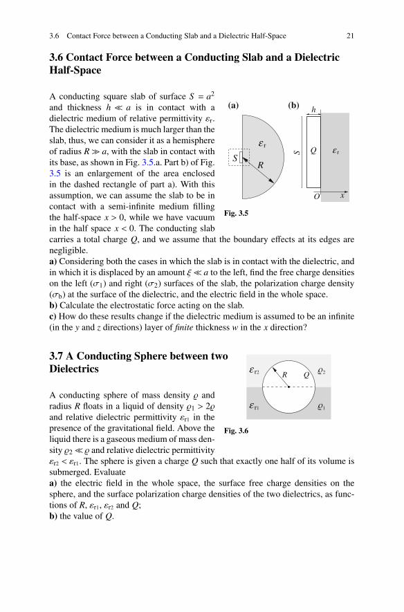
3.6 Contact Force between a Conducting Slab and a Dielectric Half-Space 21
3.6 Contact Force between a Conducting Slab and a Dielectric
Half-Space
R
ε r
S
(a)
ε rQS
h
xO
(b)
Fig. 3.5
A conducting square slab of surface S = a2
and thickness h ≪ a is in contact with a
dielectric medium of relative permittivity εr.
The dielectric medium is much larger than the
slab, thus, we can consider it as a hemisphere
of radius R≫ a, with the slab in contact with
its base, as shown in Fig. 3.5.a. Part b) of Fig.
3.5 is an enlargement of the area enclosed
in the dashed rectangle of part a). With this
assumption, we can assume the slab to be in
contact with a semi-infinite medium filling
the half-space x > 0, while we have vacuum
in the half space x < 0. The conducting slab
carries a total charge Q, and we assume that the boundary effects at its edges are
negligible.
a) Considering both the cases in which the slab is in contact with the dielectric, and
in which it is displaced by an amount ξ≪ a to the left, find the free charge densities
on the left (σ1) and right (σ2) surfaces of the slab, the polarization charge density
(σb) at the surface of the dielectric, and the electric field in the whole space.
b) Calculate the electrostatic force acting on the slab.
c) How do these results change if the dielectric medium is assumed to be an infinite
(in the y and z directions) layer of finite thickness w in the x direction?
3.7 A Conducting Sphere between two
DielectricsR 2ε r2
1ε r1
Q
Fig. 3.6
A conducting sphere of mass density and
radius R floats in a liquid of density 1 > 2
and relative dielectric permittivity εr1 in the
presence of the gravitational field. Above the
liquid there is a gaseous medium of mass den-
sity 2≪ and relative dielectric permittivity
εr2 < εr1. The sphere is given a charge Q such that exactly one half of its volume is
submerged. Evaluate
a) the electric field in the whole space, the surface free charge densities on the
sphere, and the surface polarization charge densities of the two dielectrics, as func-
tions of R, εr1, εr2 and Q;
b) the value of Q.

22 3 Electrostatics of Dielectric Media
3.8 Measuring the Dielectric Constant of a Liquid
+
−
a
b
h
g
εr
V
Fig. 3.7
A cylindrical capacitor has internal radius a,
external radius b> a, and length ℓ≫ b, so that
the boundary effects are negligible. The axis
of the capacitor is vertical, and the bottom of
the capacitor is immersed in a vessel contain-
ing a liquid of mass density and dielectric
permittivity εr, in the presence of the gravi-
tational field. If a voltage source maintains a
potential difference V between the two cylin-
drical plates, the liquid rises for a height h in
the cylindrical shell between the plates. Show
how one can evaluate the value of εr from the
measurement of h.
(This is a problem from Ref. [1]).
3.9 A Conducting Cylinder in a Dielectric Liquid
b
h
εr
Q
L
a
L−
h
Fig. 3.8
A conducting cylinder of mass M, radius a and
height L≫ a is immersed for a depth L−h (with
h≫ a) in a dielectric liquid having relative per-
mittivity εr. The liquid is contained in a cylindri-
cal vessel of radius b > a, with conducting lateral
surface. A free charge Q is located on the inter-
nal cylinder. Boundary effects are assumed to be
negligible. The cylinder is free to move vertically
preserving its axis. Find
a) the electric field E(a) at the surface of the
internal cylinder, and the surface charge densi-
ties;
b) the electric field in the region between the lat-
eral surface of the internal cylinder and the con-
tainer of the liquid (a < r < b);
c) the electrostatic force on the internal cylinder.
d) Assume that the internal cylinder has mass M,
and the liquid has mass density > M/(πa2L). Discuss the equilibrium conditions.

3.10 A Dielectric Slab in Contact with a Charged Conductor 23
3.10 A Dielectric Slab in Contact with a Charged Conductor
A dielectric slab of relative permeability εr, thickness h and surface S ≫ h is in
contact with a plane conducting surface, carrying a uniform surface charge density
σ, as in Fig. 3.9. Boundary effects are negligible.
a) Evaluate the electric field in the whole space.
b) Evaluate the polarization surface-charge densities on the dielectric surfaces.
ε r σ
S
h
conductor
Fig. 3.9
c) How do the answers to points a)
and b) change if the slab is moved
at a distance s < h from the conduct-
ing plane? How does the electrostatic
energy of the system depend on s? Is
there an interaction force between slab
and conductor?
3.11 A Transversally Polarized Cylinder
a
z
P
Fig. 3.10
An infinite cylinder of radius a has an internal
uniform electric polarization P, perpendicular
to its axis, as shown in Fig. 3.10. Evaluate the
electric charge density on the lateral surface
of the cylinder, the electric potential and the
electric field in the whole space.
Hint: see Problem 1.1.
Reference
1. J. D. Jackson, Classical Electrodynamics, John Wiley & Sons, New York,1975, Problem 4.13

Chapter 4Electric Currents
Topics. Electric current density. Continuity equation. Stationary electric currents.
Drude model for a conductor. Ohm’s law. Joule heating.
Basic equations The electric current density J = J(r, t) is the local flow of charge
per unit area and surface, which appears in the continuity equation
∂tρ +∇ ·J = 0 , (4.1)
that states the conservation of the total electric charge. In integral form
dQ
dt≡
∫V
∂tρ d3r =∫
SJ ·dS ≡ I . (4.2)
where Q is the total charge contained into the volume V bounded by the closed
surface S. Usually the flux (or electric current) I is defined also for an open surface,
as the total charge crossing the surface per unit time.
The quantity
w = J ·E (4.3)
is interpreted as the work per unit time and volume done by the EM fields on a
distribution of currents.
In a model of matter where there are several species of charged particles (labeled
with the index s) each having a charge qs, a density of particles ns = ns(r, t) and
flowing with velocity vs = vs(r, t), the current density is given by
J = ∑s
qsnsvs . (4.4)
In a metal where electrons are the only charge carrier, J = −eneve.
c© Springer International Publishing AG 2017
A. Macchi et al., Problems in Classical Electromagnetism,
DOI 10.1007/978-3-319-63133-2 4
25

26 4 Electric Currents
Drude’s model for electrons in a metal assumes the classical equation of motion
me
dve
dt= −eE−meνve , (4.5)
where ν is a phenomenological friction coefficient. In a steady state (dve/dt = 0)
this leads to Ohm’s law for a conductor
J =nee2
meνE ≡ σE ≡
E
ρ, (4.6)
where σ is the conductivity and ρ = 1/σ the resistivity of the material.1
In a material satisfying (4.6), the latter implies that the current I flowing between
two points (or layers) at different values of the electric potential, the potential drop
V is proportional to I, leading to the definition of the resistance R:
V = RI . (4.7)
In the common (but particular) example of a straight conductor of length ℓ and
cross-section area A, such that the electric field is uniform inside the conductor,
one obtains R = ℓ/(σA) = ρℓ/A. The equations (Kirchoff’s laws) describing DC
electric circuits, i.e. networks of interconnected conductors each satisfying (4.7),
can be found in any textbook and will not be repeated here.
Equation (4.7) is known as Ohm’s law, but it is appropriate to use this name
also for the underlying and more general Equation (4.6) due to G. Kirchoff. An
Ohmic conductor is defined as any material which satisfies (4.6). For such materials,
Equation (4.3) gives the power per unit volume dissipated into the material as a
consequence of the friction term,
J ·E = σE2 =E2
ρ, (4.8)
which causes the heating of the material (Joule effect). For the above mentioned
example, this is equivalent to state that the power dissipated into the whole conduc-
tor is W = RI2.
Notice that all the above equations have the same form both in the SI and in
the Gaussian system. However, the units of measure are different. For example, the
current I is measure in C/s or Ampere (1 A = 1 C/S) in SI, and in statCoulomb/s or
“statAmpere” in Gaussian units, while the resistance is measured in Ohms (Ω ) in
SI and in s/cm in Gaussian units. For the latter, σ has the dimensions of the inverse
of a time, and is thus measured in s−1, while ρ can be measured in s.
1Unfortunately the lower-case Greek letters commonly used as symbols for resistivity and con-
ductivity are the same used for volume and surface charge densities, respectively. However, the
meaning of the symbols used in the formulas throughout the book should be clear from the con-
text.

4.1 The Tolman-Stewart Experiment 27
4.1 The Tolman-Stewart Experiment
ωS
a
2b
Fig. 4.1
The experiment of Tolman and Stewart [1] was con-
ceived in order to show that conduction in metals is due
to electrons. A metallic torus (ring) of major radius a
and minor radius b is spun at a very high angular veloc-
ity ω around its axis. We assume that b ≪ a, so that the
radial motion of the charge carriers can be neglected.
The cross section of the ring is S = πb2.
At time t = 0 the rotation of the ring is suddenly
stopped. A current I = I(t) flowing in the ring and
decaying in time is observed for t > 0.
a) Using the Drude model for conduction in metals, find I = I(t) and its characteris-
tic decay time τ for a ring of copper (electrical conductivity σ ≃ 107 Ω−1m−1 and
electron density ne = 8.5×1028 m−3).
b) Evaluate the charge that flows in the ring from t = 0 to t = ∞ as a function of σ .
4.2 Charge Relaxation in a Conducting Sphere
A conducting sphere of radius a and conductivity σ has a net charge Q. At time
t = 0 the charge is uniformly distributed over the volume of the sphere, with a
volume charge density ρ0 = Q(3/4πa3). Since in static conditions the charge in
an isolated conductor can only be located on the conductor’s surface, for t > 0 the
charge progressively migrates to the surface of the sphere.
a) Evaluate the time evolution of the charge distribution on the sphere, and of the
electric field everywhere in space. Give a numerical value for the time constant τ in
the case of a good conductor (e.g., copper).
b) Evaluate the time evolution of the electrostatic energy of the sphere during the
charge redistribution.
c) Show that the energy dissipated into Joule heat equals the loss of electrostatic
energy.
4.3 A Coaxial Resistor
a
h
b
V
J
Fig. 4.2
Two coaxial cylindrical plates of very low
resistivity ρ0 have radii a and b, respectively,
with a < b. The space between the cylindrical
plates is filled up to a height h with a medium
of resistivity ρ ≫ ρ0, as in Fig. 4.2. A voltage
source maintains a constant potential differ-
ence V between the plates.

28 4 Electric Currents
a) Evaluate the resistance R of the system.
b) Discuss the relation between R and the capacitance of a cylindrical capacitor of
radii a and b.
4.4 Electrical Resistance between two Submerged Spheres (1)
a bρ
x
Fig. 4.3
a) Two highly conducting spheres of radii a
and b, respectively, are deeply submerged in
the water of a lake, at a distance x from each
other, with x ≫ a and x ≫ b. The water of the
lake has resistivity ρ . Evaluate the approx-
imate resistance between the two spheres,
using the results of the answer to point b) of
problem 4.3.
a b
ρ
x
Fig. 4.4
b) Now suppose that the two spheres are not
completely submerged, but just sunk so that
their centers are exactly at the level of the sur-
face of the lake, as shown in the figure. Eval-
uate the resistance between them.
4.5 Electrical Resistance between two Submerged Spheres (2)
ε r
ρa V
Fig. 4.5
Two identical, perfectly con-
ducting spheres of radius a are
immersed in a fluid of resis-
tivity ρ and relative electric
permittivity εr. The distance
between the centers of the two
spheres is ℓ ≫ a. A constant
potential difference difference
V is maintained between the spheres by a suitable voltage source.
As a first approximation, assume the charge to be uniformly distributed over the
surface of each sphere, neglecting electrostatic induction effects. Evaluate
a) the charge on each sphere,
b) the resistance R and the current I flowing between the spheres.
c) Find the temporal law and the decay time for the discharge of the spheres when
the voltage source is disconnected.
d) Discuss how electrostatic induction modifies the previous answers, to the lowest
order in a/ℓ.

4.6 Effects of non-uniform resistivity 29
4.6 Effects of non-uniform resistivity
Two geometrically identical cylindrical conductors have both height h and radius
a, but different resistivities ρ1 and ρ2. The two cylinders are connected in series
as in Fig. 4.6, forming a single conducting cylinder of height 2h and cross section
S = πa2. The two opposite bases are connected to a voltage source maintaining a
potential difference V through the system, as shown in the figure.
V
h h
aρ1 ρ 2
Fig. 4.6
a) Evaluate the electric fields,
the electric current and the
current densities flowing in
the two cylinders in stationary
conditions.
b) Evaluate the surface charge
densities at the surface separat-
ing the two materials, and at
the base surfaces connected to
the voltage source.
4.7 Charge Decay in a Lossy Spherical Capacitor
b
a
σ ε r
−Q0
+Q0
O
Fig. 4.7
A spherical capacitor has internal radius a
and external radius b. The spherical shell a <r < b is filled by a lossy dielectric medium
of relative dielectric permittivity εr and con-
ductivity σ . At time t = 0, the charge of the
capacitor is Q0.
a) Evaluate the time constant for the dis-
charge of the capacitor.
b) Evaluate the power dissipated by Joule
heating inside the capacitor, and compare it
with the temporal variation of the electrosta-
tic energy.
4.8 Dielectric-Barrier Discharge
The plates of a parallel-plate capacitor have surface S and separation d. The space
between the plates is divided into two layers, parallel to the plates, of thickness
d1 and d2, respectively, with d1 +d2 = d, as in Fig. 4.8. The layer of thickness d1 is
filled with a gas of negligible dielectric susceptibility (χ = 0, εr ≃ 1), while the layer
of thickness d2 is filled with a dielectric material of dielectric permittivity εr > 1.
The electric potential difference between the plates, V , is kept constant by a voltage
source. Boundary effects can be neglected.

30 4 Electric Currents
+
−d2
d1 V
ε r
Fig. 4.8
a) Find the electric field inside the capacitor.
An ionization discharge is started in the
gaseous layer at t = 0, and the gas instan-
taneously becomes conducting. We assume
that, for t > 0, the ionized gas can be consid-
ered as an Ohmic conductor of constant and
uniform resistivity ρ .
b) After a sufficiently long time we observe
that the current stops flowing in the gas, and
the system reaches a steady state (i.e., all
physical quantities are constant). Find the
electric field in the capacitor in these con-
ditions, and the surface free charge density
between the two layers.
+
−
J
d2
d1V
ε r
Fig. 4.9
c) Find the time dependence of the electric
field during the transient phase (t > 0), and
the relaxation time needed by the system to
reach the steady state condition.
4.9 Charge Distribution in a Long Cylindrical Conductor
V
0z
h−h
E
Jaρ
Fig. 4.10
Consider a conducting homogeneous
cylindrical wire of radius a and length
2h, with a ≪ h, and resistivity ρ . The
wire is connected to a voltage source
that keeps a constant potential dif-
ference V across its ends. We know
that the electric field E and, conse-
quently, the current density J = E/ρmust be uniform inside the wire, see
Problem 4.6. This implies the pres-
ence of charge distributions generat-
ing the uniform field. Only surface charge distributions are allowed in a conductor
in steady conditions. The charge distributions on the bases of the cylinder are not
sufficient for generating an even approximately uniform field in our case of a ≪ 2h.
Thus, a charge density σL must be present also on the lateral surface. Verify that a
surface charge density σL = γz, where γ is a constant and z is the coordinate along
the cylinder axis, leads to a good approximation for the field inside the conductor
far from the ends [2].

4.10 An Infinite Resistor Ladder 31
4.10 An Infinite Resistor Ladder
R
R
R
R
R
R
R
R
R
R
R
R
A
B
Fig. 4.11
An infinite resistor ladder consists
of an infinite number of resistors,
all of resistance R, arranged as in
Fig. 4.11. Evaluate the resistance mea-
sured between the terminals A and B.
Hint: use an invariance property of the
ladder.
References
1. R.C. Tolman, T.D. Stewart, The electromotive force produced by the acceleration of metals.
Phys. Rev. 8, 97–116 (1916)
2. C.A. Coombes, H. Laue, Electric fields and charge distributions associated with steady currents.
Am. J. Phys. 49, 450–451 (1981)

Chapter 5
Magnetostatics
Topics. Stationary magnetic field in vacuum. Lorentz force. Motion of an electric
point charge in a magnetic field. The magnetic force on a current. The magnetic field
of steady currents. “Mechanical” energy of a circuit in a magnetic field. Biot-Savart
law. Amperes’ circuital law. The magnetism of matter. Volume and surface magne-
tization current densities (bound currents). Magnetic susceptibility. The “auxiliary”
vector H. Magnetic field boundary conditions. Equivalent magnetic charge method.
Units. In order to write formulas compatible with both SI and Gaussian units, we
introduce two new “system dependent” constants, km and bm, defined as
km =
⎧
⎪
⎪
⎪
⎪
⎪
⎨
⎪
⎪
⎪
⎪
⎪
⎩
µ0
4π, SI,
1
c, Gaussian,
bm =
⎧
⎪
⎪
⎪
⎪
⎨
⎪
⎪
⎪
⎪
⎩
1, SI,
1
c, Gaussian,
(5.1)
where, again, µ0 = 4π×10−7 T·m/A is the “magnetic permeability of vacuum”, and
c = 29979245800 cm/s is the light speed in vacuum.
Basic equations The two Maxwell equations for the magnetic field B relevant to
this chapter are
∇ ·B = 0 , (5.2)
∇×B = 4πkm J . (5.3)
Equation (5.2) is always valid (in the absence of magnetic monopoles), while (5.3) is
valid in the absence of time-dependent electric fields. It is thus possible to introduce
a vector potential A, such that
B(r) = ∇×A(r) , (5.4)
c© Springer International Publishing AG 2017
A. Macchi et al., Problems in Classical Electromagnetism,
DOI 10.1007/978-3-319-63133-2 5
33

34 5 Magnetostatics
Imposing the gauge condition ∇ ·A = 0, the vector potential satisfies
∇2A(r) = −4πkmJ(r) , (5.5)
which is the vector analogous of Poisson’s equation (2.1). Thus,
A(r) = km
∫
V
J(r′)
|r− r′|d3r′. (5.6)
A particular and typical case is that of closed “line” currents, e.g. flowing in a
circuit having wires of negligible thickness. In such case one may replace J(r′)d3r′
by I(r′)dℓ and calculate the field via the Biot-Savart formula
B(r) = km
∮
I(r− r′)dℓ× (r− r′)
|r− r′|3, (5.7)
where the integral is extended to the closed path of the current.
The force exerted by a magnetic field over a distribution of currents is
f = bm
∫
v
J(r′)×B(r′) d3r′. (5.8)
A single point charge q located at r and moving with velocity v is equivalent to a
current density j(r′) = qδ(r− r′)v, so that the magnetic force on the point charge is
f = bmqv×B . (5.9)
The energy associated to a magnetic field distribution is given by the expression
Um =
∫
V
bmB2
8πkmµrd3r . (5.10)
In the absence of magnetic monopoles, the first non-vanishing term of the multi-
pole expansion is the magnetic dipole m
m =1
2
∫
V
r′×J(r′)d3r′. (5.11)
In the simple case of a small plane coil of area A and electric current I this reduces
to the line integral over the coil path C
m =I
2
∮
C
r′×dℓ = AIn , (5.12)

5 Magnetostatics 35
where n is perpendicular to the coil surface. A magnetic dipole term located at r = 0
generates a magnetic field
B(r) = km3r(m · r)−m
r3. (5.13)
In an external magnetic field Bext, the magnetic force on a magnetic dipole is
f = (m ·∇)Bext . (5.14)
The magnetization density M of a material is defined as the dipole moment per
unit volue,
M =dm
dV. (5.15)
Ampere equivalence theorem states that a magnetization density M=M(r) is always
equivalent to a distribution of volume current density Jm and surface current density
Km bound to the material, and given by
Jm =1
bm∇×M , (5.16)
Km =1
bmM · n , (5.17)
where n is the unit normal vector pointing outwards from the boundary surface of
the material. The total volume and surface current densities are thus
J = Jf +Jm , K =Kf +Km , (5.18)
the subscript f denoting the free (e.g., conduction) current densities.
The auxiliary field H is defined as
H =
⎧
⎪
⎪
⎪
⎪
⎨
⎪
⎪
⎪
⎪
⎩
B
µ0−M , SI,
B−4πM , Gaussian,
(5.19)
so that Equation (5.3) becomes
∇×H = 4πkm Jf , (5.20)
A material may have either a permanent magnetization, or a magnetization
induced by a magnetic field. In linear, isotropic diamagnetic and paramagnetic mate-
rials M is parallel and proportional to H,
M = χmH , (5.21)

36 5 Magnetostatics
where χm is the magnetic susceptibility of the material, with χm < 0 for diamag-
netic materials and χm > 0 for paramagnetic materials.1. The (relative) magnetic
permeability µr is defined as
µr =
1+χm , SI,
1+4πχm , Gaussian.(5.22)
We have µr < 1 for diamagnetic materials and µr > 1 for paramagnetic materials.
Inserting (5.21) and (5.22) into (5.19) we obtain
B =
µ0µr H , SI,
µr H , Gaussian,(5.23)
valid for isotropic, non-ferromagnetic, materials.
To facilitate the use of the basic equations in this chapter also with the system
independent units, we summarize some of them in the following table (Table 5.1):
Table 5.1 Basic equations for magnetostatics
Quantity SI Gaussian System independent
∇×B µ0J4π
cJ 4πkmJ
Magnetic force on a
point charge q moving
with velocity v in a
magnetic field B
qv×B qv
c×B bm qv×B
Magnetic field dB
generated by a wire
element dℓ carrying a
current I at a distance
r (Biot-Savart’s law)
µ0
4π
Idℓ× r
r2
1
c
Idℓ× r
r2km
Idℓ× r
r2
Magnetic moment m
of a ring circuit
carrying an electric
current I, and
enclosing a surface S
IS1
cI S bm I S
Volumetric magnetic
energy density um
B2
2µ0µr
B2
8πµr
bmB2
8πkmµr
1The magnetization is expressed in terms of the auxiliary field H, rather than in terms of the
magnetic field B, for historical reasons. In ferromagnetic materials there is no one-to-one corre-
spondence between M and H (between M and B) because of magnetic hysteresis

5.1 The Rowland Experiment 37
5.1 The Rowland Experiment
a
ω
b
V
a
h
h
+−
Fig. 5.1
This experiment by Henry
A. Rowland (1876) aimed at
showing that moving charges
generate magnetic fields. A
metallic disk or radius a and
thickness b ≪ a is electrically
charged and kept in rotation
with a constant angular veloc-
ity ω.
a) The disk rotates between
two conducting plates, one at a distance h ≃ 0.5 cm above its upper surface, and
the other at h below its lower surface, as in Fig. 5.1. The two plates are connected to
the same terminal of a voltage source maintaining a potential difference V0 = 104 V,
while the other terminal is connected to the disk by a sliding contact. Evaluate the
surface charge density on the disk surfaces.
b) Calculate the magnetic field Bc near the center of the disk and the magnetic field
component Br parallel and close to the disk surfaces, as a function of the distance r
from the axis. Typical experimental values were a = 10 cm, and ω ≃ 2π×102 rad/s
(period T = 2π/ω = 10−2 s).
c) The field component Br generated by the disk at r = a can be measured by ori-
enting the apparatus so that r is perpendicular to the Earth’s magnetic field B⊕, of
strength B⊕ ≃ 5× 10⁻⁵ T, and measuring the deviation of a magnetic needle when
the disk rotates. Find the deviation angle of the needle.
5.2 Pinch Effect in a Cylindrical Wire
a−e
J
Fig. 5.2
A uniform current density J
flows in an infinite cylindri-
cal conductor of radius a. The
current carriers are electrons
(charge −e) of number volume
density ne and drift velocity v,
parallel to the axis of the cylin-
der. Ions can be considered as fixed in space, with uniform number density ni and
charge Ze. The system is globally neutral.
a) Evaluate the magnetic field generated by the current, and the resulting magnetic
force on the electrons.

38 5 Magnetostatics
The magnetic force modifies the volume distribution of the electrons and this, in
turn, gives origin to a static electric field. At equilibrium the magnetic force on the
electrons is compensated by the electrostatic force.
b) Evaluate the electric field that compensates the magnetic force on the electrons,
and the corresponding charge distribution.
c) Evaluate the effect in “standard” conditions for a good Ohmic conductor.
5.3 A Magnetic Dipole in Front of a Magnetic Half-Space
x
m
−dO
y
µr
1 2
Fig. 5.3
The plane x = 0 divides the space into two half-
spaces, labeled 1 and 2, respectively. We have vac-
uum in half-space 1, while half-space 2 is filled by
a medium of magnetic permittivity µr. A magnetic
dipole m, parallel to the y axis, is located in vacuum
at position x = −d. Find
a) the magnetic field B in the whole space,
b) the force acting on the magnetic dipole.
5.4 Magnetic Levitation
In a given region of space we have a static magnetic field, which, in a cylindrical
reference frame (r,φ,z), is symmetric around the z axis, i.e., is independent of φ,
and can be written B = B(r,z). The field component along z is Bz(z) = B0z/L, where
B0 and L are constant parameters.
a) Find the radial component Br close to the z axis.
A particle of magnetic polarizability α (such that it acquires an induced magnetic
dipole moment m = αB in a magnetic field B), is located close to the z axis.
b) Find the potential energy of the particle in the magnetic field.
c) Discuss the existence of equilibrium positions for the particle, and find the fre-
quency of oscillations for small displacements from equilibrium either along z or r
(let M be the mass of the particle).
5.5 Uniformly Magnetized Cylinder
A magnetically “hard” cylinder of radius R and height h, with R ≪ h, carries a
uniform magnetization M parallel to its axis.

5.5 Uniformly Magnetized Cylinder 39
a) Show that the volume magnetization current density Jm is zero inside the cylin-
der, while the lateral surface of the cylinder carries a surface magnetization current
density Km, with |Km| = |M|.
b) Find the magnetic field B inside and outside the cylinder, at the limit h→∞.
c) Now consider the opposite case of a “flat” cylinder, i.e., h≪ R, and evaluate the
magnetic field B0 at the center of the cylinder.
d) According to the result of c), limR/h→∞B0 = 0. Obtain the same result using the
equivalent magnetic charge method.
5.6 Charged Particle in Crossed Electric and Magnetic Fields
B +
−
S hUV radiation
Ve−
Fig. 5.4
A particle of electric charge q and
mass m is initially at rest in the pres-
ence of a uniform electric field E and a
uniform magnetic field B, perpendicu-
lar to E.
a) Describe the subsequent motion of
the particle.
b) Use the above result to discuss the
following problem. We have a parallel-plate capacitor with surface S , plate sepa-
ration h and voltage V , as in Fig. 5.4. A uniform magnetic field B is applied to
the capacitor, perpendicular to the capacitor electric field, i.e., parallel to the plates.
Ultraviolet radiation causes the negative plate to emit electrons with zero initial
velocity. Evaluate the minimum value of B for which the electrons cannot reach the
positive plate.
5.7 Cylindrical Conductor with an Off-Center Cavity
ab
J
h
Fig. 5.5
An infinite cylindrical conductor of radius a has a
cylindrical cavity of radius b bored parallel to, and
centered at a distance h < a − b from the cylinder
axis as in Fig. 5.5, which shows a section of the
conductor. The current density J is perpendicular to,
and uniform over the section of the conductor (i.e.,
excluding the cavity!). The figure shows a section of
the conductor. Evaluate the magnetic field B, show-
ing that it is uniform inside the cavity.

40 5 Magnetostatics
5.8 Conducting Cylinder in a Magnetic Field
A conducting cylinder of radius a and height h≫ a rotates around its axis at constant
angular velocity ω in a uniform magnetic field B0, parallel to the cylinder axis.
h
ωB0
a
Fig. 5.6
a) Evaluate the magnetic force acting on the con-
duction electrons, assuming ω = 2π × 102 s−1 and
B = 5× 10⁻⁵ T (the Earth’s magnetic field), and the
ratio of the magnetic force to the centrifugal force.
Assume that the cylinder is rotating in stationary
conditions. Evaluate
b) the electric field inside the cylinder, and the vol-
ume and surface charge densities;
c) the magnetic field B1 generated by the rotation
currents inside the cylinder, and the order of magni-
tude of B1/B0 (assume a ≈ 0.1m).
5.9 Rotating Cylindrical Capacitor
a
−Q
ω
b
z
h
Q
Fig. 5.7
The concentric cylindrical shells of a cylindrical
capacitor have radii a and b > a, respectively, and
height h ≫ b. The capacitor charge is Q, with +Q
on the inner shell of radius a, and −Q on the outer
shell of radius b, as in Fig. 5.7. The whole capacitor
rotates about its axis with angular velocity ω = 2π/T .
Boundary effects are negligible.
a) Evaluate the magnetic field B generated by the
rotating capacitor over the whole space.
b) Evaluate the magnetic forces on the charges of the
two rotating cylindrical shells, and compare them to
the electrostatic forces.
5.10 Magnetized Spheres
a) A sphere of radius R has a uniform and permanent magnetization M. Calculate
the magnetic field inside and outside the sphere. (Hint: see Problem 3.3.)
b) A sphere of radius R has a total charge Q uniformly distributed on its surface.
The sphere rotates with angular velocity ω. Calculate the magnetic field inside and
outside the sphere.

5.10 Magnetized Spheres 41
c) A sphere of radius R has a magnetic permeability µr and is located in an external,
uniform magnetic field B0. Calculate the total magnetic field inside and outside
the sphere, discussing the limit of a perfectly diamagnetic material (µr = 0), as a
superconductor.

Chapter 6
Magnetic Induction and Time-Varying Fields
Topics. Magnetic induction. Faraday’s law. Electromotive force. The slowly varying
current approximation. Mutual inductance and self-inductance. Energy stored in an
inductor. Magnetically coupled circuits. Magnetic energy. Displacement current and
the complete Maxwell’s equations.
Basic equations In the presence of a time-varying magnetic field, Equation (1.5) is
modified into the exact equation
∇×E = −bm∂tB , (6.1)
so that the line integral of ∇×E around a closed path C is
∮
C
E ·dℓ = −bm
∫
S
∂tB ·dS (6.2)
Thus, for a fixed path, the line integral of E equals the time derivative of the flux of
the time-varying field B through a surface delimited by the contour C.
The electromotive force (emf) E in a real circuit having moving parts is the work
done by the Lorentz force on a unit charge over the circuit path,
E =
∮
circ
(E+bmV×B) ·dℓ ≡ −bmd
dtΦcirc(B) , (6.3)
where V is the velocity of the circuit element; now in (6.3) the flux Φcirc(B) of B
through the circuit may vary because of both the temporal variation of B and of the
circuit geometry. Equation (6.3) is the general Faraday’s law of induction.
For a system of two electric circuits, the magnetic flux through each circuit can
be written as a function of the currents flowing in each circuit,
Φ2 = L1I1+M21I2 , Φ1 = L2I2+M12I1 , (6.4)
c© Springer International Publishing AG 2017
A. Macchi et al., Problems in Classical Electromagnetism,
DOI 10.1007/978-3-319-63133-2 6
43

44 6 Magnetic Induction and Time-Varying Fields
where the terms containing the (self-)inductance coefficients Li are the contribution
to flux generated by the circuit itself, and the terms containing the mutual inductance
coefficients M21 = M12 give the flux generated by one circuit over the other.
Finally, for time-varying fields the complete Maxwell’s equation replacing (5.3)
is
∇×B = 4πkm J+km
ke∂tE =
⎧
⎪
⎪
⎪
⎨
⎪
⎪
⎪
⎩
4π
cJ+
1
c∂tE (Gaussian),
μ0J+μ0ε0∂tE (SI.)(6.5)
6.1 A Square Wave Generator
B
ωt
Oa
y
x
ω
Fig. 6.1
We have a uniform magnetic field B = B z in the
half space x < 0 of a Cartesian coordinate system,
while the field is zero for x > 0. A semicircular
loop of radius a and resistance R lyes in the xy
plane, with the center of the full circumference at
the origin O of our coordinate system, as in Fig.
6.1. The loop rotates around the z axis at constant
angular velocity ω.
First, assume that the self-inductance of the coil
is negligible and evaluate
a) the current circulating in the coil;
b) the torque exerted by the magnetic forces on the
coil, and the mechanical power needed to keep the
coil in rotation. Compare this to the electric power dissipated in the coil.
c) Now consider the presence of the self-inductance of the coil, and discuss how it
affects the answer to point a).
6.2 A Coil Moving in an Inhomogeneous Magnetic Field
aR
z
B(r, z)
Fig. 6.2
A magnetic field has rotational symmetry around
a straight line, that we choose as the longitudinal
axis, z, of a cylindrical reference frame (r,φ,z). The
z component of the field on the z axis, Bz(0,z), is
known and equals Bz(0,z) = B0 z/L, where L is a
constant. A circular coil has radius a, resistance R,
and axis coinciding with the z axis of our reference
frame. The coil performs a translational motion at
constant velocity v = v z, and its radius a is assumed
to be small enough that the magnetic field is always
approximately uniform over the surface limited by
the coil.

6.2 A Coil Moving in an Inhomogeneous Magnetic Field 45
a) Find the current I flowing in the coil.
b) Find the power P dissipated by the coil due to Joule heating, and the correspond-
ing frictional force f on the coil.
c) Calculate f as the resultant magnetic force on the loop carrying the
current I.
6.3 A Circuit with “Free-Falling” Parts
In the presence of the Earth’s gravitational field g, two high-conducting bars are
located vertically, at a distance a from each other. A uniform, horizontal magnetic
field B is perpendicular to the plane defined by the vertical bars. Two horizontal
bars, both of mass m, resistance R/2 and length a, are constrained to move, without
friction, with their ends steadily in contact with the two vertical bars. The resistance
of the two fixed vertical bars is assumed to be much smaller than R/2, so that the
net resistance of the resulting rectangular circuit is, with very good approximation,
always R, independently of the positions of the two horizontal bars.
R 2
R 2
B
R 2
R 2
1
2
g
aa
B
Fig. 6.3
First, assume that the upper horizontal
bar is fixed, while the lower bar starts a
“free” fall at t = 0. Let’s denote by v =
v(t) the velocity of the falling bar at time
t, with v(0) = 0.
a) Write the equation of motion for the
falling bar, find the solution for v(t)
and show that, asymptotically, the bar
approaches a terminal velocity vt.
b) Evaluate the power dissipated in the
circuit by Joule heating when v(t) = vt,
and the mechanical work done per unit
time by gravity in these conditions.
Now consider the case in which, at t = 0,
the upper bar already has a velocity v0 0
directed downwards, while the lower bar
starts a “free” fall.
c) Write the equations of motion for both
falling bars, and discuss the asymptotic behavior of their velocities v1(t) and v2(t),
and of the current in the circuit I(t).

46 6 Magnetic Induction and Time-Varying Fields
6.4 The Tethered Satellite
M
r
h
R
Fig. 6.4
The Earth’s magnetic field at the Earth’s sur-
face roughly approximates the field of a mag-
netic dipole placed at the Earth’s center. Its
magnitude ranges from 2.5 × 10⁻⁵ to 6.5 ×
10−5 T (0.25 to 0.65 G in Gaussian units),
with a value Beq ≃ 3.2×10⁻⁵ T at the equator.
A satellite moves on the magnetic equatorial
plane with a velocity v ≃ 8km/s at a constant
height h ≃ 100km over the Earth’s surface, as
shown in the figure (not to scale!). A tether
(leash, or lead line), consisting in a metal cable of length ℓ = 1 km, hangs from the
satellite, pointing to the Earth’s center.
a) Find the electromotive force on the wire.
b) The satellite is traveling through the ionosphere, where charge carriers in outer
space are available to close the circuit, thus a current can flow along the wire.
Assume that the ionosphere is rigidly rotating at the same angular velocity as the
Earth. Find the power dissipated by Joule heating in the wire and the mechanical
force on the wire as a function of its resistance R.
6.5 Eddy Currents in a Solenoid
˜
µr
I0 cosωt
R
σ z
Fig. 6.5
A long solenoid consists of a helical coil
of n turns per unit length wound around a
soft ferromagnetic cylinder of radius R and
length ℓ≫ R. The ferromagnetic material has
a relative magnetic permittivity μr, and an
electrical conductivity σ. An AC current I =
I0 cosωt flows in the coil.
a) Find the electric field induced in the
solenoid.
b) Explain why the cylinder warms up and evaluate the dissipated power.
c) Evaluate how the induced currents affect the magnetic field in the solenoid.
(Boundary effects and the displacement current are assumed to be negligible).

6.6 Feynman’s “Paradox” 47
6.6 Feynman’s “Paradox”
A non-conducting ring of radius R is at rest on the xy plane, with its center at the
origin of the coordinate system. The ring has mass m, negligible thickness, and an
electric charge Q distributed uniformly on it, so that the ring has a linear charge
density λ = Q/(2πa). The ring is free to rotate around its axis without friction.
B
B
R
x
y
λ
a
I(t)
Fig. 6.6
A superconducting circular ring of radius a≪
R, coaxial to the charged ring and carrying an
electric current I0, also lies on the xy plane, as
in Fig. 6.6. At time t = 0 the superconducting
loop is heated above its critical temperature,
and switches to normal conductivity. Conse-
quently, its current decays to zero according
to a law I = I(t).
a) Neglecting self-induction effects, evaluate
the angular velocity ω = ω(t) of the charged
ring as a function of the current I(t) in the
smaller ring. Evaluate the final angular veloc-
ity ωf , and the final angular momentum Lf , of the charged ring.
b) Evaluate the magnetic field at the ring center, Bc, generated by the rotation of the
ring.
c) Discuss how the results of a) are modified by taking the “self-inductance” L of
the charged ring into account.
This is one of the possible versions of the so-called Feynman’s disc paradox
[2], presented in Vol. II, Section 17-4, of The Feynman’s Lectures on Physics. The
apparent paradox arises because the initial total mechanical angular momentum of
the system is zero, no external torque is applied, and one could (wrongly) expect the
final total angular momentum to be zero, i.e., no rotation of the ring. This conclusion
is wrong, of course, for reasons further discussed in Prob. 8.8.
6.7 Induced Electric Currents in the Ocean
A fluid flows with uniform velocity v in the presence of a constant and uniform
magnetic field B perpendicular to v. The fluid has an electrical conductivity σ and
volumetric mass density .
a) Evaluate the electric current density J induced in the fluid.
b) Give a numerical estimate of |J| for the terrestrial oceans, knowing that the Earth’s
magnetic field has an average value B ≃ 0.5G = 5×10⁻⁵ T, the conductivity of sea
water is σ ≃ 4Ω−1m−1 (σ ≃ 3.6× 10¹⁰ s−1cm−1 in Gaussian units), and a typical
value of the flow velocity is v = 1m/s.
c) Due to the presence of the induced current, the magnetic force tends to slow down
the fluid. Estimate the order of magnitude for the time constant of this effect.

48 6 Magnetic Induction and Time-Varying Fields
6.8 A Magnetized Sphere as Unipolar MotorR
V−
+
AB
M
ω
P
z
aO
Fig. 6.7
A magnetized, non-conducting sphere has radius a,
mass m and permanent, uniform magnetization M
throughout its volume. An electric circuit is formed
by pasting a conducting wire along a half meridian,
from the pole P to the equator, and another conduct-
ing wire around the whole equator of the sphere, as
shown in Fig. 6.7. The circuit is closed by two brush
contacts (the white arrows in Fig. 6.7) connecting the
pole P, and a point A of the wire on the equator of
the sphere, to a voltage source of electromotive force
V . The resulting circuit has resistance R.
a) Evaluate the torque on the sphere when a current I flows in the circuit.
b) If the sphere is free to rotate without friction around the z axis of a cylindrical
coordinate system, parallel to M and passing through the center O of the sphere, it
reaches asymptotically a terminal angular velocity ωt. Evaluated ωt and the charac-
teristic time of the system.
6.9 Induction Heating
Consider a homogeneous material of electrical conductivity σ and relative mag-
netic permeability μr, both real, positive and independent of frequency. The electric
permittivity is εr = 1.
a) Show that, if the displacement current density ∂tE/(4πke) can be neglected, the
magnetic field B inside the material obeys the equation
∂tB = α∇2B , (6.6)
and determine the value of the real constant α.
The material fills the half-space x > 0 in the presence of a uniform oscillating
magnetic field B0 = y B0 cos(ωt) = y Re(
B0 e−iωt)
in the half-space x < 0.
b) Evaluate the magnetic field B(x, t) for x > 0, assuming that the displacement cur-
rent is negligible. Discuss under what conditions the result is a good approximation
for the case of a finite slab of the material.
c) Evaluate the power dissipated in the medium by Joule heating.
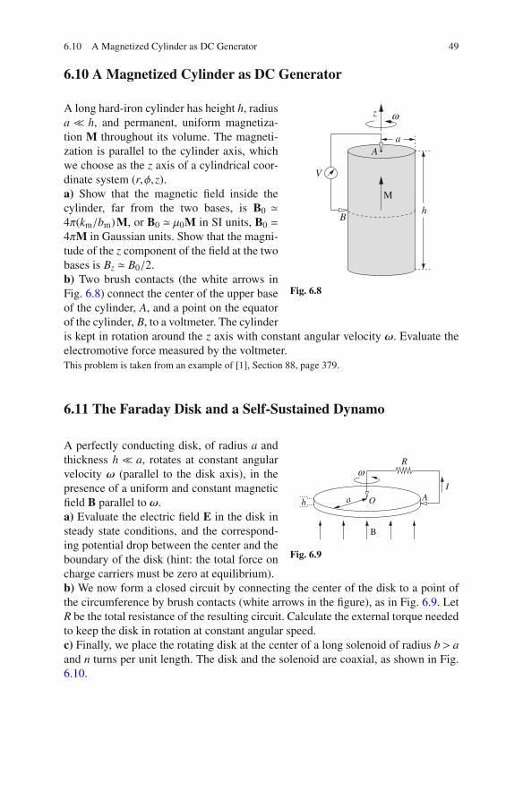
6.10 A Magnetized Cylinder as DC Generator 49
6.10 A Magnetized Cylinder as DC Generator
M
h
a
B
ω
V
A
z
Fig. 6.8
A long hard-iron cylinder has height h, radius
a ≪ h, and permanent, uniform magnetiza-
tion M throughout its volume. The magneti-
zation is parallel to the cylinder axis, which
we choose as the z axis of a cylindrical coor-
dinate system (r,φ,z).
a) Show that the magnetic field inside the
cylinder, far from the two bases, is B0 ≃
4π(km/bm)M, or B0 ≃ μ0M in SI units, B0 =
4πM in Gaussian units. Show that the magni-
tude of the z component of the field at the two
bases is Bz ≃ B0/2.
b) Two brush contacts (the white arrows in
Fig. 6.8) connect the center of the upper base
of the cylinder, A, and a point on the equator
of the cylinder, B, to a voltmeter. The cylinder
is kept in rotation around the z axis with constant angular velocity ω. Evaluate the
electromotive force measured by the voltmeter.
This problem is taken from an example of [1], Section 88, page 379.
6.11 The Faraday Disk and a Self-Sustained Dynamo
R
B
I
a Ah O
ω
Fig. 6.9
A perfectly conducting disk, of radius a and
thickness h ≪ a, rotates at constant angular
velocity ω (parallel to the disk axis), in the
presence of a uniform and constant magnetic
field B parallel to ω.
a) Evaluate the electric field E in the disk in
steady state conditions, and the correspond-
ing potential drop between the center and the
boundary of the disk (hint: the total force on
charge carriers must be zero at equilibrium).
b) We now form a closed circuit by connecting the center of the disk to a point of
the circumference by brush contacts (white arrows in the figure), as in Fig. 6.9. Let
R be the total resistance of the resulting circuit. Calculate the external torque needed
to keep the disk in rotation at constant angular speed.
c) Finally, we place the rotating disk at the center of a long solenoid of radius b > a
and n turns per unit length. The disk and the solenoid are coaxial, as shown in Fig.
6.10.

50 6 Magnetic Induction and Time-Varying Fields
ωa
B
B
Rb
Fig. 6.10
The two brush contacts of point b) are now
connected to the ends of the solenoid coil,
so that the rotating disk provides the current
circulating in the turns. The total resistance
of the disk-solenoid circuit is R. The circu-
lating current is thus due to the disk rotation
and to the presence of the magnetic field B,
that the current itself generates by circulating
in the solenoid (self-sustained dynamo). Find
the value of ω for steady-state conditions.
This is an elementary model for a dynamo
self-sustained by rotation, such as the gener-
ation mechanism of the Earth’s magnetic field [3].
6.12 Mutual Induction between Circular Loops
b
y
a ωO
I
x
B
A
Fig. 6.11
The centers of two circular conducting loops
A and B, of radii a and b ≫ a, respectively,
are located at the origin O of a Cartesian ref-
erence frame. At time t = 0 both loops lie on
the xy plane. While the larger loop remains at
rest, the smaller loop, of resistance R, rotates
about one of its diameters, lying on the x
axis, with angular velocity ω, as shown in
Fig. 6.11. A constant current I circulates in
the larger loop.
a) Evaluate the current IA induced in loop A,
neglecting self-inductance effects.
b) Evaluate the power dissipated in loop A due to Joule heating.
c) Evaluated the torque needed to keep loop A in rotation, and the associated
mechanical power.
d) Now consider the case when loop A is at rest on the xy plane, with a constant
current I circulating in it, while loop B rotates around the x axis with constant
angular velocity ω. Evaluate the electromotive force induced in B, neglecting self-
inductance effects.
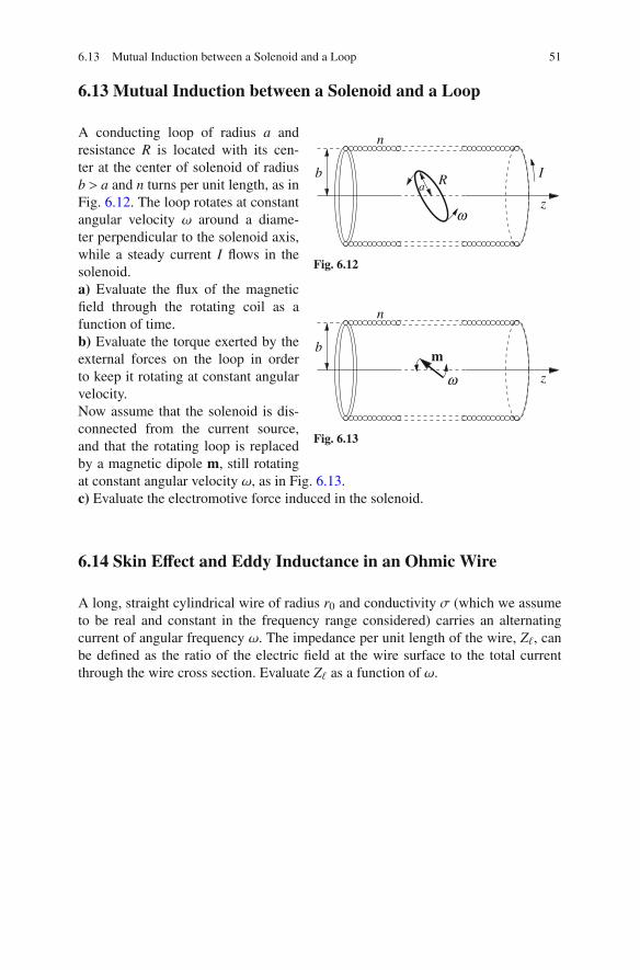
6.13 Mutual Induction between a Solenoid and a Loop 51
6.13 Mutual Induction between a Solenoid and a Loop
z
ba
R
n
ω
I
Fig. 6.12
A conducting loop of radius a and
resistance R is located with its cen-
ter at the center of solenoid of radius
b > a and n turns per unit length, as in
Fig. 6.12. The loop rotates at constant
angular velocity ω around a diame-
ter perpendicular to the solenoid axis,
while a steady current I flows in the
solenoid.
z
b
n
m
ω
Fig. 6.13
a) Evaluate the flux of the magnetic
field through the rotating coil as a
function of time.
b) Evaluate the torque exerted by the
external forces on the loop in order
to keep it rotating at constant angular
velocity.
Now assume that the solenoid is dis-
connected from the current source,
and that the rotating loop is replaced
by a magnetic dipole m, still rotating
at constant angular velocity ω, as in Fig. 6.13.
c) Evaluate the electromotive force induced in the solenoid.
6.14 Skin Effect and Eddy Inductance in an Ohmic Wire
A long, straight cylindrical wire of radius r0 and conductivity σ (which we assume
to be real and constant in the frequency range considered) carries an alternating
current of angular frequency ω. The impedance per unit length of the wire, Zℓ, can
be defined as the ratio of the electric field at the wire surface to the total current
through the wire cross section. Evaluate Zℓ as a function of ω.

52 6 Magnetic Induction and Time-Varying Fields
6.15 Magnetic Pressure and Pinch effect for a Surface Current
K
a
z
Fig. 6.14
A current I flows on the surface of a cylinder of
radius a and infinite length, in the direction parallel
to the axis z. The current layer has negligible thick-
ness, so that we can write I = 2πaK, with K = Kz the
surface current density. Calculate
a) the magnetic field B in the whole space,
b) the force per unit surface P on the cylinder surface
c) the variation of magnetic field energy (per unit
length) dUm associated to an infinitesimal variation
of the radius da. Explain why P −(2πa)−1dUm/da
and how to calculate P correctly from the energy
variation.
Notice: for point b) it might be useful to show first
that for a magnetostatic field we have
J×B =1
4πkm
[
(B ·∇)B−12∇B2]
. (6.7)
6.16 Magnetic Pressure on a Solenoid
A current source supplies a constant current I to a solenoid of radius a, length h≫ a,
so that boundary effects are negligible, and n coils per unit length.
a) Evaluate the magnetic pressure on the solenoid surface directly, by computing
the magnetic force on the coils.
b) Now evaluate the magnetic pressure on the solenoid surface by evaluating the
variation of the magnetic energy of the system for an infinitesimal increase da of
the radius of the solenoid, and the corresponding work done by the current source
in order to keep I constant.

6.17 A Homopolar Motor 53
6.17 A Homopolar Motor
II
circuitz
magnet
+
−A
LK
AL
INE
CE
LL
M
Fig. 6.15
circuitB
magnet
cell
II
−
+
M
Fig. 6.16
A homopolar motor is a direct current electric motor
consisting of a circuit carrying a direct current I in
the presence of a static magnetic field. The circuit is
free to rotate around a fixed axis, so that the angle
between the current and the magnetic field remains
constant in time in each part of the circuit. The
resulting electromotive force is continuous, and the
homopolar motor needs no device, like a commuta-
tor, to switch the current flow. But it still requires
slip rings (or brush contacts) to operate. “Homopo-
lar” means that the electrical polarity of the conduc-
tor (the direction of the current flow at each point of
the circuit) and the magnetic field do not change in
time, and the motor does not require commutation. A
simple practical realization of a homopolar motor is
shown in Figs. 6.15 and 6.16, based on a Wikipedia
entry.
The idea is the following: an electrochemical cell
drives a DC current into the double circuit shown in
the figures, while a magnetic field is generated gen-
erated by the permanent magnet cylindrical located
at the bottom of the cell, in electrical contact with its
negative pole, as shown in Fig. 6.16. The magnetic
field has rotational symmetry around the z axis and
is constant in time, in spite of the magnet rotation,
and the circuit is free to rotate around the z axis. The
magnetic forces on the current-carrying circuit exert a torque, and the circuit starts
to rotate.
The dimensions, mass and resistance of the circuit (the mass includes battery and
magnet), the voltage of the battery and the magnetic field strength generated by the
magnet at each point of the circuit are known. Find the torque acting on the circuit,
and the angular velocity of the system as a function of time,
References
1. R. Becker, Electromagnetic Fields and Interactions, vol. I (Electromagnetic Theory and Rela-
tivity, Blackie, London and Glasgow, 1964)
2. R. P. Feynman, R. B. Leighton, M. Sands, The Feynman Lectures on Physics, Addison-Wesley
Publishing Company, Reading, MA, 2006. Volume II, Section 17-4
3. R. T. Merrill, Our magnetic Earth: the Science of Geomagnetism, Chapter 3, Chicago Univer-
sity Press, 2010

Chapter 7
Electromagnetic Oscillatorsand Wave Propagation
Topics Harmonic oscillators. Resonances. Coupled oscillators, normal modes and
eigenfrequencies. Basics of the Fourier transform. Electric circuits:
impedances, simple LC and RLC circuits. Waves. The wave equation. Monochro-
matic waves. Dispersion. Wavepackets. Phase velocity and group velocity. Trans-
mission lines.
Useful formulas for this chapter:
Fourier transform of the Gaussian function
∫ +∞−∞
e−(αk)2
eikxdk =
√π
αe−x2/4α2
, (7.1)
where in general α is a complex number with Re(α) > 0.
c© Springer International Publishing AG 2017
A. Macchi et al., Problems in Classical Electromagnetism,
DOI 10.1007/978-3-319-63133-2 7
55
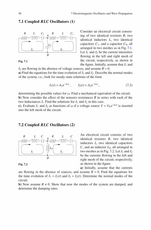
56 7 Electromagnetic Oscillators and Wave Propagation
7.1 Coupled RLC Oscillators (1)
C0
C1LR R C1
B
L
I1 I2
A
Fig. 7.1
Consider an electrical circuit consist-
ing of two identical resistors R, two
identical inductors L, two identical
capacitors C1, and a capacitor C0, all
arranged in two meshes as in Fig. 7.1.
Let I1 and I2 be the current intensities
flowing in the left and right mesh of
the circuit, respectively, as shown in
the figure. Initially, assume that I1 and
I2 are flowing in the absence of voltage sources, and assume R = 0.
a) Find the equations for the time evolution of I1 and I2. Describe the normal modes
of the system, i.e., look for steady-state solutions of the form
I1(t) = A1e−iωt , I2(t) = A2e−iωt , (7.2)
determining the possible values for ω. Find a mechanical equivalent of the circuit.
b) Now consider the effect of the nonzero resistances R in series with each of the
two inductances L. Find the solutions for I1 and I2 in this case.
c), Evaluate I1 and I2 as functions of ω if a voltage source V = V0 e−iωt is inserted
into the left mesh of the circuit.
7.2 Coupled RLC Oscillators (2)
CL RR
B
LA
C
L0
I1 I2
Fig. 7.2
An electrical circuit consists of two
identical resistors R, two identical
inductors L, two identical capacitors
C, and an inductor L0, all arranged in
two meshes as in Fig. 7.2. Let I1 and I2
be the currents flowing in the left and
right mesh of the circuit, respectively,
as shown in the figure.
a) Initially, assume that the currents
are flowing in the absence of sources, and assume R = 0. Find the equations for
the time evolution of I1 = I1(t) and I2 = I2(t). Determine the normal modes of the
circuit.
b) Now assume R 0. Show that now the modes of the system are damped, and
determine the damping rates.

7.3 Coupled RLC Oscillators (3) 57
7.3 Coupled RLC Oscillators (3)
R R RL L L
C CI3I2I1
A
B
D
E
Fig. 7.3
An electrical circuit consists
of three identical resistors R,
three identical inductors L,
and two identical capacitors C,
arranged in three meshes as in
Fig. 7.3. Let I1, I2, and I3 be the
currents flowing in the three
meshes, as in the figure. Ini-
tially, assume R = 0.
a) Write the equations for the time evolution of In(t). Find a mechanical system with
three degrees of freedom and the same equations of motion as those for In(t).
b) Determine the normal oscillation modes of the system and their frequencies.
c) Now assume R 0, and determine the decay rate of the normal modes.
7.4 The LC Ladder Network
InIn−2 In+1
. . . . . .
In−1
L C Qn−1 Qn+1Qn
A
B
F
E G
D
a
Fig. 7.4
An LC ladder network is
formed by N inductors L, and
N capacitors C, arranged as
shown in Fig. 7.4. We denote
by In = In(t) the current in
the nth inductor. Resistance
effects are assumed to be neg-
ligible. The distance between
two neighboring nodes is a.
a) Find the equations for the time evolution of In. Which is a mechanical equivalent
of the system?
b) Show that solutions exist in the form of propagating monochromatic waves
In =C ei(kna−ωt) (7.3)
and find the dispersion relation between k and ω.
c) For a given value of ω, find the allowed values of k with the boundary conditions
I0 = IN = 0.
d) Discuss the limit to a continuum system, N→∞, n→∞, a→ 0, with na→ x. In
this case inductance and capacity are continuously distributed, i.e., defined per unit
length.

58 7 Electromagnetic Oscillators and Wave Propagation
7.5 The CL Ladder Network
Vn
. . .L
C
Qn−1 QnQn+1
Vn−1 Vn+1
In−1 In In+1
. . .
Fig. 7.5
Consider an infinite ladder network of
identical capacitors C and inductors
L, arranged as shown in Fig. 7.5. Let
Qn = Qn(t) be the charge on the nth
capacitor, Vn = Vn(t) the voltage drop
on the nth inductor, and In = In(t) =
dQn/dt is the current flowing in the
nth mesh, across the nth capacitor, i.e., between the network nodes at Vn−1 and
Vn.
a) Show that the currents In satisfy the coupled equations
Ld2
dt2(In+1−2In+ In−1) =
In
C. (7.4)
b) Show that the solutions of (7.4) have the form
In = Aei(kna−ωt) , (7.5)
with a the distance between two adjacent network elements, and determine the dis-
persion relation ω = ω(k).
7.6 Non-Dispersive Transmission Line
R
d
L = 1/GCLR
x x + x
Fig. 7.6
The “elementary cell”
scheme of a transmis-
sion line is sketched in
the figure. In addition
to the inductance L and
capacitance C typical of
the ideal “LC” trans-
mission line, there is a resistance R in series with L, which accounts for the finite
resistivity of the two conductors which form the line. In addition, we assume a finite
leakage of current between the two conductors (i.e., in the direction “transverse”
to the propagation) which is modeled by a second resistance RL in parallel to C.
The corresponding conductance is G = 1/RL. In the limit of a continuous system
with homogeneous, distributed properties, we define all quantities per unit length
by replacing R with Rℓdx, L with Lℓdx, C with Cℓdx and G with Gℓdx (it is proper
to use G as a quantity defined per unit length instead of RL because the latter is
proportional to the inverse of the length of the line).

7.6 Non-Dispersive Transmission Line 59
a) Show that the current intensity I = I(x, t) satisfies the equation
(∂2x −LℓCℓ∂
2t )I = (RℓCℓ +LℓGℓ)∂tI+RℓGℓI = 0 . (7.6)
b) Study the propagation of a monochromatic current signal of frequency ω, i.e.,
search for solutions
I = I0eikx−iωt , (7.7)
for x > 0 with the boundary condition I(0, t) = I0e−iωt, and determine the dispersion
relation k = k(ω).
c) Find the condition on the line parameters for which a wavepacket traveling along
the lines undergoes attenuation of the amplitude but no dispersion. This condition
corresponds to solutions having the general form
I(x, t) = e−κx f (x− vt) , (7.8)
where f (x) is an arbitrary differentiable function. Find the expression for v and κ.
7.7 An “Alternate” LC Ladder Network
L1 L2 L1 L2
C C CI2n I2n+1I2n−1 I2n+2
Fig. 7.7
Consider an “alternate” LC ladder network comprising identical capacitors C and
inductors of value alternatively L1 and L2, as shown in Fig. 7.7. Let I2n be the current
flowing in the mesh of the nth inductor of value L2, and I2n+1 the current flowing in
the n-th inductor of value L1.a) Show that the currents satisfy the equations
L2d2I2n
dt2=
1
C(I2n−1 −2I2n + I2n+1) , L1
d2I2n+1
dt2=
1
C(I2n −2I2n+1 + I2n+2) . (7.9)
What is a mechanical equivalent of this network?
b) Search for solutions of (7.9) of the form
I2n = Ie ei [2nka−ωt] , I2n+1 = Io ei [(2n+1)ka−ωt] , (7.10)

60 7 Electromagnetic Oscillators and Wave Propagation
where Ie and Io (the subscripts “e” and “o” stand for even and odd, respectively)
are two constants, and determine the dispersion relation ω = ω(k). Determine the
allowed frequency range for wave propagation (for simplicity, assume L2≪ L1).
7.8 Resonances in an LC Ladder Network
Consider the semi-infinite LC ladder network shown in Fig. 7.8. Let In = In(t) be the
current flowing in the n-th mesh of the circuit. An ideal current source provides the
input current
I(t) = Ise−iωt, (7.11)
where
a) Assuming ω < 2ω0, evaluate In(t) as a function of Is and ω.
b) Now find In(t) assuming ω > 2ω0. Hint: search for a solution of the form
In(t) = Aαne−iωt, (7.12)
determining the dependence of α on ω and ω0.
L
CI(t) I0 I1 I2 In
Fig. 7.8
L
CI(t) IN−1I1 I2I0
Fig. 7.9
Now assume that our LC ladder is finite, comprising N meshes numbered from
0 to N − 1, as in Fig. 7.9. Evaluate In(t) both for the case ω > 2ω0 and for the case
ω < 2ω0, determining for which values of ω resonances are observed.
7.9 Cyclotron Resonances (1)
Consider a particle of charge q and mass m in the presence of a constant, uniform
magnetic field B= B0 z, and of a uniform electric field of amplitude E0, rotating with
frequency ω in the (x,y) plane, either in clockwise or in counterclockwise direction
(Fig. 7.10 shows the counterclockwise case).
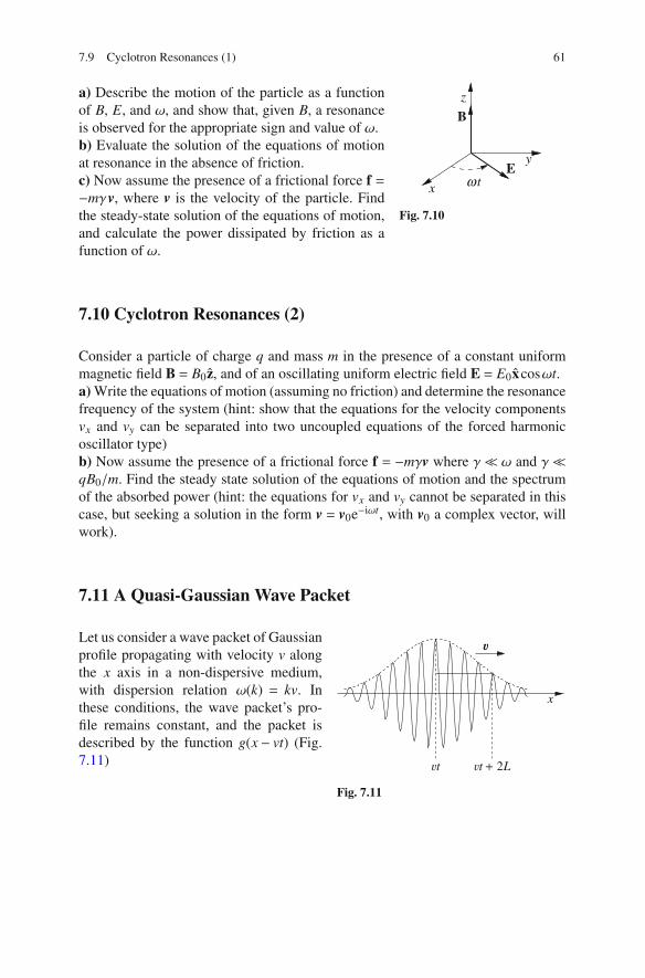
7.9 Cyclotron Resonances (1) 61
ω tE
y
z
x
B
Fig. 7.10
a) Describe the motion of the particle as a function
of B, E, and ω, and show that, given B, a resonance
is observed for the appropriate sign and value of ω.
b) Evaluate the solution of the equations of motion
at resonance in the absence of friction.
c) Now assume the presence of a frictional force f =
−mγv, where v is the velocity of the particle. Find
the steady-state solution of the equations of motion,
and calculate the power dissipated by friction as a
function of ω.
7.10 Cyclotron Resonances (2)
Consider a particle of charge q and mass m in the presence of a constant uniform
magnetic field B = B0z, and of an oscillating uniform electric field E = E0xcosωt.
a) Write the equations of motion (assuming no friction) and determine the resonance
frequency of the system (hint: show that the equations for the velocity components
vx and vy can be separated into two uncoupled equations of the forced harmonic
oscillator type)
b) Now assume the presence of a frictional force f = −mγv where γ≪ ω and γ≪qB0/m. Find the steady state solution of the equations of motion and the spectrum
of the absorbed power (hint: the equations for vx and vy cannot be separated in this
case, but seeking a solution in the form v = v0e−iωt, with v0 a complex vector, will
work).
7.11 A Quasi-Gaussian Wave Packet
x
t t + 2L
Fig. 7.11
Let us consider a wave packet of Gaussian
profile propagating with velocity v along
the x axis in a non-dispersive medium,
with dispersion relation ω(k) = kv. In
these conditions, the wave packet’s pro-
file remains constant, and the packet is
described by the function g(x − vt) (Fig.
7.11)

62 7 Electromagnetic Oscillators and Wave Propagation
g(x− vt) =√π
A
Leik0(x−vt)e−(x−vt)2/4L2
=
∫ +∞−∞
g(k)eik(x−vt)dk, (7.13)
where L, A and k0 are constant parameters, and g(k) = Ae−(k−k0)2L2is the Fourier
transform of g. Now consider a second wave packet described by a function f ,
whose Fourier transform is
f (k) = g(k)eiφ(k) = Ae−(k−k0)2L2
eiφ(k) , (7.14)
where the “phase perturbation” φ(k) is a smooth function, that can be approximated
by its Taylor polynomial expansion of degree 2 around k = k0,
φ(k) ≃ φ(k0)+φ′(k0)(k− k0)+1
2φ′′(k0)(k− k0)2 , (7.15)
where φ′ and φ′′ are the first and second derivatives of φ. The second wave packet
can be considered as an “attempt” to build up a Gaussian wave packet from its
spectral components, but with some error on the relative phases of the components
themselves. Find the width of the wave packet and discuss its shape in order to show
its deviations from the Gaussian profile.
7.12 A Wave Packet along a Weakly Dispersive Line
A transmission line extends from x = 0 to x = +∞. A generator at x = 0 inputs a
signal
f (t) = Ae−iω0te−t2/τ2 , (7.16)
where A and τ are constant and ω0τ≫ 1, i.e., the signal is “quasi-monochromatic”.
The dispersion relation of the transmission line can be written
ω = ω(k) = kv (1+bk) , (7.17)
where v and b are known constants, and we assume k > 0.
a) Find the expression f (x, t) for the propagating signal, i.e., for the wave packet
traveling along the line, assuming b = 0.
From now on, assume dispersive effects to be small but not negligible, i.e.,
assume bk0≪ 1, where k0 = k(ω0) according to (7.17).
b) Within the above approximation, write the phase and group velocities as functions
of ω0 to the lowest order at which dispersive effects are present.

7.12 A Wave Packet along a Weakly Dispersive Line 63
c) Give an estimate of the instant tx when the “peak” of the signal reaches the posi-
tion x, and of the corresponding length of the wave packet.
d) Now find the expression of the wave-packet shape as a function of (x, t), by
calculating the integral
f (x, t) =
∫eik(ω)x−iωt f (ω)dω, (7.18)
where f (ω) is the Fourier transform of the wave packet. As a reasonable approxi-
mation, keep only factors up to the second order in (k− k0)2, for instance use
k(ω) ≃ k(ω0)+ k′(ω0)(ω−ω0)+1
2k′′(ω0)(ω−ω0)2. (7.19)

Chapter 8
Maxwell Equations and Conservation Laws
Topics Maxwell’s equations. Conservation laws: energy, momentum and angular
momentum of the electromagnetic field. Poynting’s theorem. Radiation pressure.
Basic equations of this chapter:
(Note: Gaussian cgs units are used in this chapter unless otherwise specified.)
Maxwell’s equations
∇ ·E = 4πρ , (8.1)
∇ ·B = 0 , (8.2)
∇×E = −1
c∂tB , (8.3)
∇×B =4π
cJ+
1
c∂tE . (8.4)
Energy conservation (Poynting’s) theorem
∂tu+∇ ·S = −J ·E , (8.5)
where
u =1
8π
(
E2+B2)
(8.6)
is the energy density of the EM field, and
S =c
4πE×B (8.7)
is the Poynting (also named Poynting-Umov) vector.
c© Springer International Publishing AG 2017
A. Macchi et al., Problems in Classical Electromagnetism,
DOI 10.1007/978-3-319-63133-2 8
65

66 8 Maxwell Equations and Conservation Laws
Momentum conservation theorem:
∂tg+∇ ·T = −
(
ρE+1
cJ×B
)
, (8.8)
where
g =1
4πc(E×B) =
S
c2(8.9)
is the momentum density of the EM field, and T is Maxwell’s stress tensor with
components
Ti j =1
4π
[
1
2(E2+B2)δi j−EiE j−BiB j
]
. (8.10)
Thus, ∇ ·T is a vector with components
(∇ ·T)i =
j=3∑
j=1
∂ jTi j . (8.11)
Angular momentum density of an EM field
ℓ = r×g = r×S
c. (8.12)

8.1 Poynting Vector(s) in an Ohmic Wire 67
8.1 Poynting Vector(s) in an Ohmic Wire
A constant and uniformly distributed current density J = σE flows inside an infinite
straight wire of radius a and conductivity σ.
a) Calculate the Poynting vector S = (c/4π)E×B and discuss the energy conserva-
tion in the wire.
b) The Poynting vector occurs in Poynting’s theorem only through its divergence,
since the theorem only requires that the flux of the Poynting vector through any a
closed surface describes the net flow of electromagnetic energy. Show that, conse-
quently, S′ = ϕJ, where ϕ is the electrostatic potential, is also a suitable choice for
S (hint: substitute E = −∇ϕ into (8.7) and manipulate the result).
8.2 Poynting Vector(s) in a Capacitor
a
h E
Fig. 8.1
A plane capacitor consists of two par-
allel circular plates of radius a, at a
distance h ≪ a from each other. The
electric field inside the capacitor is
slowly varying in time, E = E(t) z, for
instance, assume E = E0 t/τ. Bound-
ary effects are negligible (Fig. 8.1).
a) Evaluate the magnetic field B inside
the capacitor.
b) Calculate the Poynting vector S= (c/4π)E×B, and show that the flux of S though
any surface enclosing the capacitor equals the time variation of the energy associated
to the electromagnetic field.
c) Show that an alternative Poynting vector is
S′ =1
4πϕ∂tE , (8.13)
where ϕ is the electric potential (E = −∇ϕ). Verify that also the flux of S′ through
the closed surface of point b) equals the variation of the energy in the volume inside
the surface [hint: proceed as in point b) of Problem 8.1].
8.3 Poynting’s Theorem in a Solenoid
A time-dependent current, I = I(t) = I0 t/τ, flows through the coils of an infinitely
long, cylindrical solenoid. The solenoid has radius a and n turns per unit length.
a) Find the magnetic and electric fields, B and E, inside the solenoid.

68 8 Maxwell Equations and Conservation Laws
b) Verify the law of energy conservation (Poynting’s theorem), for a closed internal
cylindrical surface, coaxial to the solenoid.
c) Now verify Poynting’s theorem for an external, coaxial cylindrical surface
(remember that B = 0 outside an infinite solenoid).
8.4 Poynting Vector in a Capacitor with Moving Plates
−
+
(−Q0)
(V0)
(+Q0)
h(t)
a
Fig. 8.2
A plane capacitor consists of two circular
metallic plates of radius a, parallel to each
other. One plate is kept at rest while the other
moves at constant velocity v, so that the dis-
tance between the plates is h = h(t) = h0 + vt.
In the following we consider only the case in
which h ≪ a at any time t, so that bound-
ary effects are negligible. We also assume
that v is small enough to ensure the valid-
ity of the slowly varying current approxi-
mation7.11 A Quasi-Gaussian Wave Packet
(Fig. 8.2).
Considering both the case of electrically isolated plates having opposite charges
±Q0, and the case of plates connected through a voltage source keeping a constant
electric potential drop V0 between them, calculate
a) the force F needed to keep v constant,
b) the rate of change of the electrostatic energy U,
c) the magnetic field between the plates,
d) the Poynting vector S and its flux through a cylindrical surface enclosing, and
coaxial with, the capacitor; use this last result to discuss energy conservation in the
system.
8.5 Radiation Pressure on a Perfect Mirror
A perfect mirror is defined as a medium inside which E = 0 and B = 0. Thus, an EM
wave cannot penetrate the mirror surface and will be reflected by it.
Find the radiation pressure Prad, i.e., the cycle–averaged force per unit surface
exerted by a plane wave incident on the surface of a perfect plane mirror, as a func-
tion of the intensity I of the wave by each of the following three methods:
a) Consider the reflection of a square wave packet of arbitrary, but finite, duration.
Determine Prad from the difference between the total momentum of the incident
wave packet and the momentum of the reflected wave packet.

8.5 Radiation Pressure on a Perfect Mirror 69
b) Calculate the force on the mirror directly, from the knowledge of the EM fields
and of the charge and current densities on the mirror surface.
c) Determine Prad from Maxwell’s stress tensor.
8.6 A Gaussian Beam
In optics, a Gaussian beam is a beam of monochromatic electromagnetic radiation
whose transverse magnetic and electric field amplitude profiles are given by the
Gaussian function. Gaussian beams are important because they are a very good
approximation of the radiation emitted by most laser sources. Here we consider
a linearly-polarized Gaussian beam propagating along the z-axis and whose trans-
verse profile is symmetrical around such axis. The origin of the coordinate systems
is chosen so that the beam has minimum width on the z = 0 plane. We assume that,
close to the z= 0 plane, the transverse components of the EM fields can be written as
Ex = E0(r)cos(kz−ωt) = E0 e−r2/r20 cos(kz−ωt),
By = B0(r)cos(kz−ωt) = B0 e−r2/r20 cos(kz−ωt), (8.14)
where r =√
x2+ y2 < r0 and k = ω/c. The parameter r0 is called the waist of the
beam.
a) Show that, in addition to the transverse components (8.14), longitudinal compo-
nents Ez and Bz must exist, and give their expression.
b) Compute the Poynting vector of the beam S, and its average over a period 〈S〉,
showing which components are vanishing.
c) Verify that the fields (8.14) do not satisfy the wave equation in vacuum, hence
they are only an approximate expression, as mentioned above. Explain in which
range of z, depending on the value of kr0, the approximate expressions are accurate.
8.7 Intensity and Angular Momentum of a Light Beam
A circularly polarized monochromatic light beam of frequency ω propagates along
the z direction. The beam has a finite width in the plane perpendicular to z. We
assume that in a region of space, close to the “waist” (i.e., to the plane where the
beam has minimal width), the transverse components of the EM fields can be written
approximately as
Ex = +E0(r)cos(kz−ωt) , Ey = −E0(r) sin(kz−ωt) ,
Bx = E0(r) sin(kz−ωt) , By = E0(r)cos(kz−ωt) , (8.15)
where r =√
x2+ y2, k = ω/c, and E0(r) is a known real function.

70 8 Maxwell Equations and Conservation Laws
a) Write the intensity I = I(r), defined as the “energy flow along z”, i.e., I(r) = S z =
S · z where S is the Poynting vector.
b) Show that, in addition to the transverse components of the fields, also longitudinal
components (Ez, Bz) must exist, and give their expression.
c) Evaluate the S x and S y component of S, and discuss the result.
d) Show that the density of angular momentum (8.12) of the beam can be written as
ℓz = ℓz(r) = −r
2cωdrI , (8.16)
and compute the quantity
Lz =
∫ ∞
0
ℓz(r)2πr dr (8.17)
as a function of the total power of the beam W =∫ ∞
0I(r)2πr dr.
8.8 Feynman’s Paradox solved
B0
a
h
σ=
Q/(2
πah)
λ=
Q/h
Fig. 8.3
The system in Fig. 8.3 is composed by a non-
conducting cylindrical surface of height h and
radius a, over which there is a net charge
Q uniformly distributed with surface density
σ = Q/(2πah), and a wire of same length
oriented along the cylinder axis and having
charge −Q distributed with uniform linear
density λ = −Q/h, so that the system is glob-
ally neutral. The cylindrical surface is free to
rotate around its axis without friction, and has
moment of inertia I per unit length. The sys-
tem is at rest in the presence of an external
uniform magnetic field Bext, parallel to the system axis. Assume that boundary
effects can be neglected.
Starting at time t = 0, the external magnetic field is reduced from its initial value
Bext = B0 to zero at a time t f ≫ a/c, according to some temporal law Bext = Bext(t).
a) Initially assuming that the field generated by the motion of the charges on the
cylinder is negligible, evaluate the angular velocity ω = ω(t) of the cylinder as a
function of time during the decay of Bext, and the corresponding mechanical angular
momentum Lc of the cylinder.
b) Now take the field generated by rotating charges into account, and evaluate how
the results of a) change.
c) Consistently with Eqs. (8.8–8.9), we introduce the angular momentum of a given
distribution of electromagnetic fields as

8.8 Feynman’s Paradox solved 71
LEM =
∫
r×gd3r , (8.18)
where g = E×B/4π is the electromagnetic momentum density. Use Eq. (8.18) to
check the conservation of the total angular momentum for the system (thus solving
the “paradox” as outlined in Problem 6.6).
8.9 Magnetic Monopoles
Assume that an experiment gives evidence of the existence of “magnetic monopoles”,
i.e., of point-like particles with a net magnetic charge qm, such that the magnetic
field Bm generated by such charge is
Bm = αqm
r2r , (8.19)
while in the presence of an “external” magnetic field Bext the force on the particle
is f = qmBext. Thus, for example, the interaction force between two particles with
magnetic charges qm1 and qm2 is given by
f1→2 = αqm1qm2
r212
r12 , f2→1 = −f1→2 . (8.20)
where r12 is the distance vector directed from charge 1 to charge 2. We also assume
that conservation of the total magnetic charge holds.
a) Determine, both in SI and Gaussian units, the expressions for the coefficient α
and the dimensions of the magnetic charge qm with respect to the electric charge
qe. (Hint: we may assume that the field generated by two magnetic charges +qm
and −qm, separated by a distance h, is equivalent to the field of a magnetic dipole
m = qmh at distances r≫ |h|.)
b) Complete Maxwell’s equations in order to take the presence of magnetic monopoles
into account.
c) Now consider a beam of magnetic monopoles of radius a, of uniform density and
infinite length. The number density of the particles of the beam is n, and all particles
have the same magnetic charge qm and the same velocity v. Find the electric and
magnetic fields generated by the beam.

Chapter 9
Relativistic Transformations of the Fields
Topics Relativistic covariance of Maxwell’s equations. Four-vectors in electromag-
netism: four-current, four-potential. The electromagnetic four-tensor. Lorentz trans-
formations of the fields.
Basic equations of this chapter:
Relation of four-current and four-potential to densities and potentials in three-
dimensional space
Jµ ≡ (ρc,J) , Aµ = (φ,A) . (9.1)
Lorentz transformations of a four-vector Kµ = (K0,K) from the frame S to the
frame S ′ moving with relative velocity v = βc with respect to S :
K′0 = γ(K0−β ·K) , K′‖= γ(K‖−βK0) , K′⊥ =K⊥ , (9.2)
where the subscripts “‖” and “⊥” denote the directions parallel and perpendicular to
β, respectively, and γ = 1/√
1−β2.
Compact three-dimensional formulas for the transformation of the EM fields are
E′‖= E‖ , E′⊥ = γ(E⊥+β×B) , B′
‖= B‖ , B′⊥ = γ(B⊥−β×E) , (9.3)
or, equivalently
E′ = γ (E+β×B)−γ2
γ+1β(β ·E) , (9.4)
B′ = γ (B−β×E)−γ2
γ+1β(β ·B) . (9.5)
The three-dimensional “Newtonian” force transforms as
c© Springer International Publishing AG 2017
A. Macchi et al., Problems in Classical Electromagnetism,
DOI 10.1007/978-3-319-63133-2 9
73

74 9 Relativistic Transformations of the Fields
F′‖= F‖−
VF · v⊥/c2
1−Vv‖/c2, F′⊥ =
F⊥
γ(1−Vv‖/c2), (9.6)
where V is the boost velocity, and v‖ and v⊥ are the components of the particle
velocity parallel and perpendicular to V, respectively. We have F = dp/dt in the S
frame and F′ = dp′/dt′ in the S ′ frame.
9.1 The Fields of a Current-Carrying Wire
I
Sr
vq
Fig. 9.1
In the laboratory frame S , a constant current I
flows in an infinitely long wire. The wire has
no net charge density. A test charge q moves
with a velocity v parallel to the current at a
distance r from the wire, as shown in Fig. 9.1.
a) Find the force F acting on q in the labora-
tory frame. Then evaluate the force F′ acting
on the charge in the reference frame S ′ where
the charge is at rest, applying the appropri-
ate Lorentz transformation. What can be inferred on the EM fields in S ′ from the
expression of F′?
b) Use the Lorentz transformations to obtain the charge and current densities of the
wire in S ′, and the related EM fields. Evaluate the scalar and vector potentials in S ′.
Compare the results to what obtained from the direct transformation rules for the
EM field.
c) The answers to points a) and b) imply that in S ′ there is a net charge density on
the wire. Recover this result by calculating the linear densities of electrons (flowing
with velocity ve in S ) and ions (at rest in S ) in S ′ via the Lorentz transformations
for velocity and length. (this last point corresponds to the one presented by E.M.
Purcell in Ref. [1].)
9.2 The Fields of a Plane Capacitor
O x
zy
Lh
Q
−Q
L
S
S
Fig. 9.2
In the laboratory frame S , a plane capaci-
tor has parallel square plates of area A = L2,
located at a distance h≪ L from each other,
so that the boundary effects can be assumed
to be negligible. The plates have electric
charges ±Q, uniformly distributed over their
surfaces, with surface charge density ±σ =
±Q/A, respectively (Fig. 9.2).
Evaluate, in a reference frame S ′ moving with respect to S with velocity v = βc
parallel to the capacitor plates,

9.2 The Fields of a Plane Capacitor 75
a) the electric and magnetic fields in the region between the plates;
b) the sources of the fields;
c) the force per unit surface and the total force on each plate, comparing the results
to the corresponding values in S .
9.3 The Fields of a Solenoid
I
I
n
q
R
Fig. 9.3
In the laboratory frame S a constant current I flows
in an infinite solenoid of radius R and n turns per
unit length. At a given instant t = 0 a test particle of
charge q is located inside the solenoid, with a veloc-
ity v perpendicular to the axis of the solenoid, as
shown in Fig. 9.3.
a) Find the electromagnetic fields and the force on
the particle both in S , and in the frame S ′ where the
particle is instantaneously at rest (v′ = 0).
b) Assuming v/c≪ 1, evaluate the sources of the fields in S ′ up to the first order in
v/c.
9.4 The Four-Potential of a Plane Wave
Consider a monochromatic plane wave, propagating in vacuum along the x axis of
the Cartesian laboratory frame S , linearly polarized along y, and of frequency ω.
a) Show that the electric field E = E(x, t) and the magnetic field B = B(x, t) of the
wave can be obtained from a suitable four-potential Aµ = (Φ,A) = (0,0,Ay,0).
Now consider the same wave observed in a frame S ′, moving with velocity v = v y
with respect to S .
b) Evaluate the frequency ω′ and the wave vector k′ of the wave in S ′. Calculate the
electric field E′ = E′(r′, t′) and the magnetic field B′ = B′(r′, t′) in S ′ as functions
of E in the S frame.
c) Verify that the wave is linearly polarized in S ′ and show that E′ and B′ can be
obtained from a four-potential A′µ = (0,A′), where A′ = A′(r′, t′).
d) Find the four-potential A′µ obtained from Aµ through a Lorentz transformation.
Verify that E′ and B′ can be obtained also from A′µ.
e) Show that A′µ and A′µ are related by a gauge transformation.
9.5 The Force on a Magnetic Monopole
Assume that an experiment has given evidence for the existence of magnetic
monopoles, i.e., point-like particles which, in the presence of a magnetic field B,
are subject to a force
Fm = qmB , (9.7)

76 9 Relativistic Transformations of the Fields
where qm is the magnetic charge of the monopole. We assume that these particles
have no electric charge.
a) Show that the force exerted by an electric field E on a monopole moving in the
laboratory frame with velocity v is
Fe = −qmv
c×E . (9.8)
b) The “Lorentz force” on a magnetic monopole is the sum of (9.7) and (9.8). Use
this expression to study the motion of a magnetic monopole of mass m in either an
electric field E or in perpendicular E and B fields, where the fields are both constant
and uniform, and E > B. For simplicity assume a non-relativistic motion. Compare
the results to those of Problem 5.6, point a).
9.6 Reflection from a Moving Mirror
An electromagnetic wave of frequency ω and electric field amplitude Ei, linearly
polarized along the y axis, is perpendicularly incident on a perfect conductor whose
bounding surface lies on the yz plane. The perfect conductor behaves as a perfect
mirror, i.e., we have E = 0 and B = 0 inside the material (x > 0).
a) Evaluate the the field of the reflected wave and the total electromagnetic field.
The mirror is now set in motion with respect to the laboratory frame S , with a
constant velocity v = xv parallel to the x axis.
b) Find the frequencies and the fields of the incident and reflected waves in the S ′
frame, where the mirror is at rest.
c) Find the frequency and the fields of the reflected wave in the S frame.
d) Discuss the continuity of the fields at the moving mirror surface.
9.7 Oblique Incidence on a Moving Mirror
kr ,ω
r
k i,ωi
θr
θi
Fig. 9.4
In the laboratory frame S , a perfectly reflecting mir-
ror moves with constant velocity v, perpendicular to
its surface. In S , the wave vector ki of an incident
EM wave makes an angle θi with the normal to the
mirror surface, as in Fig. 9.4. The incident wave has
frequency ωi. Find
a) the frequency ω′i
of the incident wave, the inci-
dence angle θ′i, and the reflection angle θ′r in the in
the S ′ frame, where the mirror is at rest;
b) the frequency ωr of the reflected wave, and the
reflection angle θr, in the S frame. What happens if
cosθi v/c?

9.8 Pulse Modification by a Moving Mirror 77
9.8 Pulse Modification by a Moving Mirror
N
Fig. 9.5
In the laboratory frame S we have an EM square
wave packet of amplitude Ei, comprising N com-
plete oscillations of frequency ωi, therefore of dura-
tion τi = 2πN/ωi. Assume that N ≫ 1, so that the
packet is “quasi-monochromatic”. The wave packet
impinges perpendicularly on a perfect mirror. In the
laboratory frame, the mirror itself is moving with
constant velocity v perpendicularly to its surface
(Fig. 9.5).
a) Determine the form, duration and amplitude of the reflected wave packet.
b) Compare the total energies of the incident and reflected wave packets, and deter-
mine the amount of mechanical work W done by the mirror during the reflection
stage (consider all quantities per unit surface).
c) Show that W is equal to the integral over time and volume of J ·E, in agreement
with Poynting’s theorem.
9.9 Boundary Conditions on a Moving Mirror
x
y
z
Ei
x(t)
k
Fig. 9.6
The reflecting surface of a perfect
mirror is parallel to the yz plane of a
laboratory Cartesian reference frame
S . The mirror is translating with con-
stant velocity v parallel to the x axis,
as in Fig. 9.6. A plane monochromatic
wave of frequency ωi, amplitude Ei,
and wave vector ki = xωi/c, linearly
polarized along the y axis, impinges
onto the mirror.
a) Show that in the laboratory frame S both total (i.e., incident + reflected) fields
E and B are discontinuous at the mirror surface, lying on the plane x = x(t), with
dx/dt = v.
b) The EM fields can be derived from a vector potential A(x, t). Show that the bound-
ary conditions for the EM fields at the mirror surface are equivalent to the condition
d
dtA[x(t), t] = 0 , (9.9)
which states that the value of the vector potential at the surface is constant (i.e.,
time-independent) in the laboratory frame.

78 9 Relativistic Transformations of the Fields
c) As a consequence of (9.9), we can assume A[x(t), t] ≡ 0. Use this boundary con-
dition to obtain the frequency (ωr) and amplitude (Er) of the reflected wave in the
laboratory frame.
Reference
1. E.M. Purcell, Electricity and Magnetism (Berkeley Physics Course—Vol. 2, Section 5.9), 2nd
edn. (McGraw-Hill Book Company, New York, 1984)

Chapter 10
Radiation Emission and Scattering
Topics The radiation field. Multipole expansion. Electric dipole radiation. Magnetic
dipole radiation.
Basic equations of this chapter:
Fields in the radiation zone of a point-like source at r = 0 having an electric dipole
moment p(t):
E(r, t) =
[
p(tret)× r]
× r
rc2, B(r, t) = r×E (10.1)
where tret = t− r/c.
Instantaneous radiation power from the electric dipole source and its angular distri-
bution
Prad =2
3c3|p|2 ,
dPrad
dΩ=
3Prad
4πsin2 θ , (10.2)
where θ is the angle between p and r, and the infinitesimal solid angle dΩ =
2πsinθdθ.
Analogous formulas for the fields and the power of a magnetic dipole m(t):
E(r, t) = −[m(tret)× r]
rc2, B(r, t) = r×E , (10.3)
Prad =2
3c3|m|2 ,
dPrad
dΩ=
3Prad
4πsin2 θ . (10.4)
10.1 Cyclotron Radiation
An electron moves in the xy plane in the presence of a constant and uniform
magnetic field B = B0 z. The initial velocity is v0 ≪ c, so that the motion is non-
c© Springer International Publishing AG 2017
A. Macchi et al., Problems in Classical Electromagnetism,
DOI 10.1007/978-3-319-63133-2 10
79
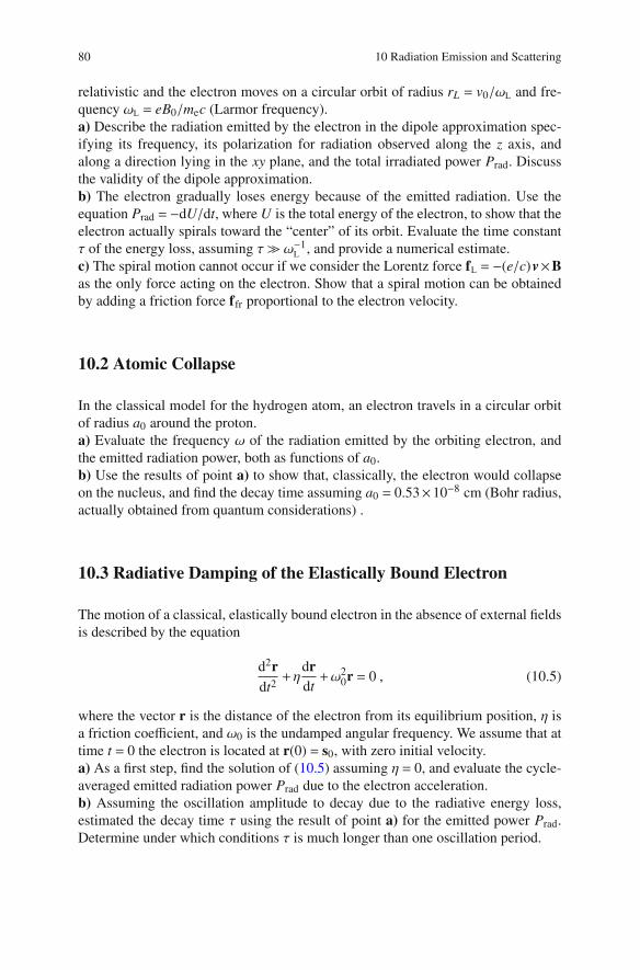
80 10 Radiation Emission and Scattering
relativistic and the electron moves on a circular orbit of radius rL = v0/ωL and fre-
quency ωL = eB0/mec (Larmor frequency).
a) Describe the radiation emitted by the electron in the dipole approximation spec-
ifying its frequency, its polarization for radiation observed along the z axis, and
along a direction lying in the xy plane, and the total irradiated power Prad. Discuss
the validity of the dipole approximation.
b) The electron gradually loses energy because of the emitted radiation. Use the
equation Prad = −dU/dt, where U is the total energy of the electron, to show that the
electron actually spirals toward the “center” of its orbit. Evaluate the time constant
τ of the energy loss, assuming τ≫ ω−1L , and provide a numerical estimate.
c) The spiral motion cannot occur if we consider the Lorentz force fL = −(e/c)v×B
as the only force acting on the electron. Show that a spiral motion can be obtained
by adding a friction force ffr proportional to the electron velocity.
10.2 Atomic Collapse
In the classical model for the hydrogen atom, an electron travels in a circular orbit
of radius a0 around the proton.
a) Evaluate the frequency ω of the radiation emitted by the orbiting electron, and
the emitted radiation power, both as functions of a0.
b) Use the results of point a) to show that, classically, the electron would collapse
on the nucleus, and find the decay time assuming a0 = 0.53×10⁻⁸ cm (Bohr radius,
actually obtained from quantum considerations) .
10.3 Radiative Damping of the Elastically Bound Electron
The motion of a classical, elastically bound electron in the absence of external fields
is described by the equation
d2r
dt2+η
dr
dt+ω2
0r = 0 , (10.5)
where the vector r is the distance of the electron from its equilibrium position, η is
a friction coefficient, and ω0 is the undamped angular frequency. We assume that at
time t = 0 the electron is located at r(0) = s0, with zero initial velocity.
a) As a first step, find the solution of (10.5) assuming η = 0, and evaluate the cycle-
averaged emitted radiation power Prad due to the electron acceleration.
b) Assuming the oscillation amplitude to decay due to the radiative energy loss,
estimated the decay time τ using the result of point a) for the emitted power Prad.
Determine under which conditions τ is much longer than one oscillation period.

10.3 Radiative Damping of the Elastically Bound Electron 81
Now assume η 0, with η≪ ω0, in Eq.(10.5). In the following, neglect quantities
of the order (η/ω0)2 or higher.
c) Describe the motion of the electron and determine, a posteriori, the value of η
that reproduces the radiative damping.
10.4 Radiation Emitted by Orbiting Charges
Two identical point charges q rotate with constant angular velocity ω on the circular
orbit x2+ y2 = R2 on the z = 0 plane of a Cartesian reference frame.
a) Write the most general trajectory for the charges both in polar coordinates ri =
ri(t), φi = φi(t) and in Cartesian coordinates xi = xi(t), yi = yi(t) (where i = 1,2 labels
the charge) and calculate the electric dipole moment of the system.
b) Characterize the dipole radiation emitted by the two-charge system, discussing
how the power depends on the initial conditions, and finding the polarization of the
radiation emitted along the x, y and z directions.
c) Answer questions a) and b) in the case where the charges are orbiting with oppo-
site angular velocity.
d) Now consider a system of three identical charges on the circular orbit with the
same angular velocity. Find the initial conditions for which the radiation power is
either zero or has its maximum.
e) Determine whether the magnetic dipole moment gives some contribution to the
radiation, for each of the above specified cases.
10.5 Spin-Down Rate and Magnetic Field of a Pulsar
α
m
ω
R
M
Fig. 10.1
A pulsar is a neutron star with mass M ≈ 1.4M⊙ ≈
2.8×1033 g (where M⊙ is the Sun mass), and radius
R ≃ 10km = 106 cm. The star rotates with angular
velocity ω and has a magnetic moment m, which is,
in general, not parallel to the rotation axis. [1]
a) Describe the radiation emitted by the pulsar, and
find the total radiated power, assuming that the angle
between the magnetic moment and the rotation axis
is α, as in Fig. 10.1.
b) Find the “spindown rate” (decay constant of the
rotation) of the pulsar, assuming that energy loss is
due to radiation only.
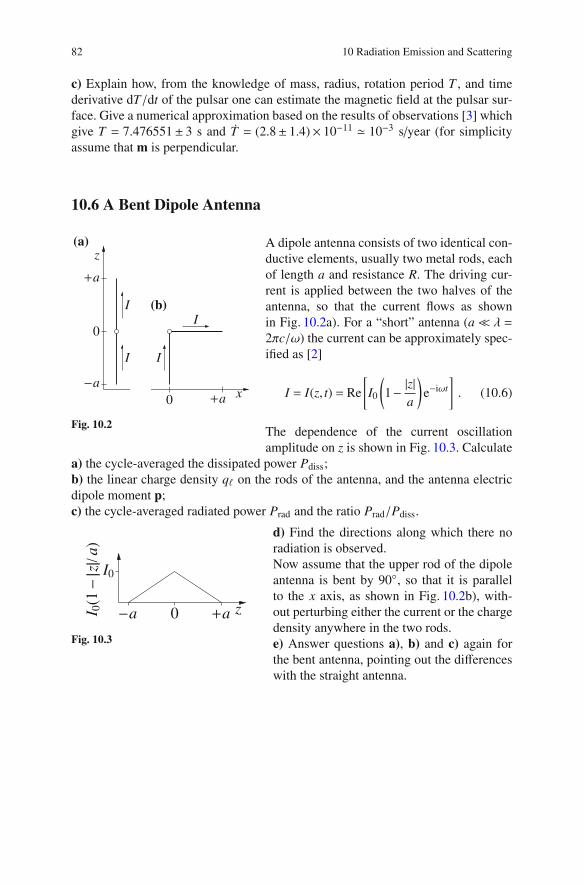
82 10 Radiation Emission and Scattering
c) Explain how, from the knowledge of mass, radius, rotation period T , and time
derivative dT/dt of the pulsar one can estimate the magnetic field at the pulsar sur-
face. Give a numerical approximation based on the results of observations [3] which
give T = 7.476551± 3 s and T = (2.8± 1.4)× 10−11 ≃ 10−3 s/year (for simplicity
assume that m is perpendicular.
10.6 A Bent Dipole Antenna
+a
−a
II
+a x
0
0
I I
(b)
z(a)
Fig. 10.2
A dipole antenna consists of two identical con-
ductive elements, usually two metal rods, each
of length a and resistance R. The driving cur-
rent is applied between the two halves of the
antenna, so that the current flows as shown
in Fig. 10.2a). For a “short” antenna (a≪ λ =
2πc/ω) the current can be approximately spec-
ified as [2]
I = I(z, t) = Re
[
I0
(
1−|z|
a
)
e−iωt
]
. (10.6)
The dependence of the current oscillation
amplitude on z is shown in Fig. 10.3. Calculate
a) the cycle-averaged the dissipated power Pdiss;
b) the linear charge density qℓ on the rods of the antenna, and the antenna electric
dipole moment p;
c) the cycle-averaged radiated power Prad and the ratio Prad/Pdiss.
I0
0−a +aI 0(1
−|z
|/a)
z
Fig. 10.3
d) Find the directions along which there no
radiation is observed.
Now assume that the upper rod of the dipole
antenna is bent by 90, so that it is parallel
to the x axis, as shown in Fig. 10.2b), with-
out perturbing either the current or the charge
density anywhere in the two rods.
e) Answer questions a), b) and c) again for
the bent antenna, pointing out the differences
with the straight antenna.
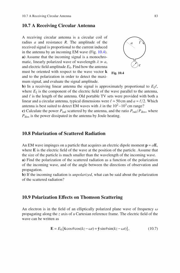
10.7 A Receiving Circular Antenna 83
10.7 A Receiving Circular Antenna
a I
ε
Fig. 10.4
A receiving circular antenna is a circular coil of
radius a and resistance R. The amplitude of the
received signal is proportional to the current induced
in the antenna by an incoming EM wave (Fig. 10.4).
a) Assume that the incoming signal is a monochro-
matic, linearly polarized wave of wavelength λ≫ a,
and electric field amplitude E0. Find how the antenna
must be oriented with respect to the wave vector k
and to the polarization in order to detect the maxi-
mum signal, and evaluate the signal amplitude.
b) In a receiving linear antenna the signal is approximately proportional to E‖ℓ,
where E‖ is the component of the electric field of the wave parallel to the antenna,
and ℓ is the length of the antenna. Old portable TV sets were provided with both a
linear and a circular antenna, typical dimensions were ℓ ≃ 50cm and a ≃ ℓ/2. Which
antenna is best suited to detect EM waves with λ in the 102−103 cm range?
c) Calculate the power Prad scattered by the antenna, and the ratio Prad/Pdiss, where
Pdiss is the power dissipated in the antenna by Joule heating.
10.8 Polarization of Scattered Radiation
An EM wave impinges on a particle that acquires an electric dipole moment p = αE,
where E is the electric field of the wave at the position of the particle. Assume that
the size of the particle is much smaller than the wavelength of the incoming wave.
a) Find the polarization of the scattered radiation as a function of the polarization
of the incoming wave, and of the angle between the directions of observation and
propagation.
b) If the incoming radiation is unpolarized, what can be said about the polarization
of the scattered radiation?
10.9 Polarization Effects on Thomson Scattering
An electron is in the field of an elliptically polarized plane wave of frequency ω
propagating along the z axis of a Cartesian reference frame. The electric field of the
wave can be written as
E = E0[
xcosθcos(kz−ωt)+ ysinθ sin(kz−ωt)]
, (10.7)

84 10 Radiation Emission and Scattering
where θ is a constant real number with 0 θ π/2. such that we have linear polar-
ization along the x axis for θ = 0, linear polarization along the y axis for θ = π/2,
and circular polarization for θ = π/4.
First, neglecting the effects of the magnetic force −ev×B/c,
a) characterize the radiation scattered by the electron by determining the frequency
and the polarization observed along each axis (x, y, z), and find a direction along
which the radiation is circularly polarized;
b) calculate the total (cycle-averaged) scattered power and discuss its dependence
on θ;
Now consider the effect of the magnetic force on the scattering process.
c) Evaluate the −ev×B/c term by calculating the B field from (10.7) and using the
result of point a) for v. Discuss the direction and frequency of the magnetic force
and its dependence on θ as well.
d) Discuss how the scattering of the incident wave is modified by the magnetic
force by specifying which new frequencies are observed, in which direction and
with which polarization, and the modification of the scattered power.
10.10 Scattering and Interference
E
x
L
−d
2
d
2
θ
y
k 0 x
P
r +
r −
Fig. 10.5
A monochromatic plane wave prop-
agates along the x axis of a Carte-
sian coordinate system. The wave is
linearly polarized in the z direction,
and has wavelength λ. Two identical,
point-like scatterers are placed on the
x axis at x = ±d/2, respectively, as in
Fig. 10.5. The dipole moment of each
scatterer is p = αE, where E is the
electric field of the incoming wave at
the scatterer position. The intensity Is of the scattered radiation is measured on the
y = L plane, with both L≫ d and L≫ λ.
a) Evaluate the phase difference Δφ between the two scattered waves in a generic
point P ≡ (x,L,0), with L a constant, as a function of the observation angle θ =
arctan(x/L), as shown in Fig. 10.5.
b) Study the scattered intensity distribution Is = Is(θ) as a function of kd, where k is
the wave vector of the incoming wave. Determine for which values of kd interfer-
ence fringes appear.

10.11 Optical Beats Generating a “Lighthouse Effect” 85
10.11 Optical Beats Generating a “Lighthouse Effect”
x
p− p+
P
O
r
zd
2
d
2
y
φ
Fig. 10.6
Two oscillating dipoles, p− and p+, are
located at (0,−d/2,0) and (0,+d/2,0), respec-
tively, in a Cartesian reference frame. The
two dipoles are parallel to the z axis and
oscillate, with equal amplitude, at slightly
different frequencies ω± = ω0 ± δω/2, with
δω≪ ω0. In complex representation we have
p± = p0 e−iω±t. The distance between the two
dipoles is d = λ0/2 = πc/ω0. The radiation
emitted by the dipoles is observed at a point
P at a distance r from the origin, with r≫ λ0,
on the z = 0 plane. Let φ be the angle between
r and the x axis, as shown in Fig. 10.6.
a) Determine the direction of the electric field in P and its dependence on φ and ω±,
up to the first order in δω/ω0.
The wave intensity in P is measured by two detectors with different temporal reso-
lutions: the first detector measures the “instantaneous” flux averaged over an inter-
val Δt such that 2π/ω0 ≪ Δt ≪ 2π/δω, while the second detector averages over
Δt′≫ 2π/δω.
b) Determine the dependence on the angle φ and the time t of the fluxes measured
with the two detectors.
c) How do the above results change if the observation point is located in the x = 0
plane?
10.12 Radiation Friction Force
An accelerated point charge emits radiation. Considering for definiteness an electron
performing a periodic (non-relativistic for simplicity) motion in an oscillating exter-
nal field, there is a finite amount of energy leaving the electron as radiation, but on
the average the external field produces no work. Thus, to account self-consistently
for the energy lost as radiation, it is necessary to modify the Newton-Lorentz force
by adding a new “friction” term Frad so that the mechanical work done by Frad
equals the radiated energy.1
We thus write for the electron
medv
dt= −e
(
E+v
c×B
)
+Frad , (10.8)
1From another viewpoint, Frad aims to describe the back-action or reaction of the self-generated
EM fields on the accelerated charge.

86 10 Radiation Emission and Scattering
and look for a suitable expression for Frad starting from the condition
∫ t+T
t
Frad(t) · v(t)dt = −
∫ t+T
t
Prad(t)dt , (10.9)
where T is the period of the electron motion and Prad(t) is the instantaneous radiated
power, which is given by the Larmor formula
Prad(t) =2e2
3c2
∣
∣
∣
∣
∣
dv
dt
∣
∣
∣
∣
∣
2
. (10.10)
a) Show by direct substitution of the expression for Frad
Frad = meτd2
v
dt2(10.11)
into (10.9), that the equation is verified, and find the expression of the constant τ,
estimating its numerical value.
b) Determine the steady state solution of (10.8), where Frad is given by (10.11), for
an electron in a uniform, oscillating electric field
E(t) = Re(
−eE0 e−iωt)
. (10.12)
Compare the result with what obtained using the simple classical model an electron
subject to a frictional force
medv
dt= Fext−meηv . (10.13)
References
1. C. Bernardini, C. Guaraldo, Fisica del Nucleo (Editori Riuniti, Roma, 1982)
2. J.D. Jackson, Classical Electrodynamics, §9.2 and 9.4, 3rd edn. (Wiley, New York, London,
Sydney, 1998)
3. C. Kouveliotou et al., An X-ray pulsar with a superstrong magnetic field in the soft γ-ray
repeater SGR1806-20. Nature 393, 235–237 (1998)
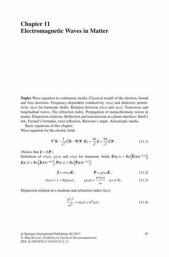
Chapter 11
Electromagnetic Waves in Matter
Topics Wave equation in continuous media. Classical model of the electron, bound
and free electrons. Frequency-dependent conductivity σ(ω) and dielectric permit-
tivity ε(ω) for harmonic fields. Relation between σ(ω) and ε(ω). Transverse and
longitudinal waves. The refraction index. Propagation of monochromatic waves in
matter. Dispersion relations. Reflection and transmission at a plane interface: Snell’s
law, Fresnel’s formulas, total reflection, Brewster’s angle. Anisotropic media.
Basic equations of this chapter:
Wave equation for the electric field:
∇2E−1
c2∂2
t E−∇(∇ ·E) =4π
c2J =
4π
c2∂2
t P . (11.1)
(Notice that J = ∂tP.)
Definition of σ(ω), χ(ω) and ε(ω) for harmonic fields E(r, t) = Re[
E(r)e−iωt]
,
J(r, t) = Re[
J(r)e−iωt]
, P(r, t) = Re[
P(r)e−iωt]
:
J = σ(ω)E , P = χ(ω)E , (11.2)
ε(ω) = 1+4πχ(ω) , χ(ω) =iσ(ω)
ω(ω 0) . (11.3)
Dispersion relation in a medium and refraction index n(ω):
k2c2
ω2= ε(ω) = n
2(ω) . (11.4)
c© Springer International Publishing AG 2017
A. Macchi et al., Problems in Classical Electromagnetism,
DOI 10.1007/978-3-319-63133-2 11
87

88 11 Electromagnetic Waves in Matter
11.1 Wave Propagation in a Conductor at High and Low
Frequencies
In a classical treatment, a metal has ne conduction electrons per unit volume, whose
equations of motion in the presence of an external electric field E(r, t) are
medv
dt= −eE(r, t)−meηv , v =
dr
dt, (11.5)
where −e and me are electron charge and mass, respectively, and η is a constant
describing friction.
a) Determine the complex conductivity of the metal, σ = σ(ω), as a function of the
angular frequency ω of the electric field, and the values of ω for which σ is either
purely real or purely imaginary. Discuss these limits for a good conductor, whose
DC conductivity (i.e., its conductivity for static fields) has values of the order of
σDC ∼ 5×10¹⁷ s−1.
Now consider a monochromatic, plane EM wave, linearly polarized along the y axis
and traveling in the positive direction along the x axis of a Cartesian coordinate
system. The wave is incident on a conductor filling the x > 0 half-space, while we
have vacuum in the x < 0 half-space.
b) Consider both cases of σ purely real and purely imaginary, and determine the
frequency ranges in which the wave is evanescent inside the metal.
c) Find the time-averaged EM energy flux through the metal surface and show that
it is equal to the amount of energy dissipated inside the metal.
11.2 Energy Densities in a Free Electron Gas
A plane, monochromatic, transverse electromagnetic wave propagates in a medium
containing ne free electrons per unit volume. The electrons move with negligible
friction. Calculate
a) the dispersion relation of the wave, the phase (vϕ) and group (vg) velocities, and
the relation between the amplitudes of the electric (E0) and magnetic (B0) fields;
b) the EM energy density uEM (averaged over an oscillation period) as a function of
E0;
c) the kinetic energy density uK (averaged over an oscillation period), defined as
uK = neme〈v2〉/2, where v is the electron oscillation velocity, and the total energy
density u = uEM+uK.
d) Assume that the medium fills the half-space x > 0, while we have vacuum in the
half-space x < 0. An EM wave, propagating along the x axis, enters the medium.
Assume that both vg and vϕ are real quantities. Use the above results to verify the
conservation of the energy flux, expressed by the relation
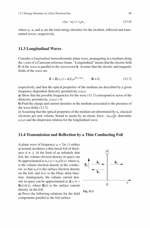
11.2 Energy Densities in a Free Electron Gas 89
c(ui−ur) = vgut , (11.6)
where ui, ur and ut are the total energy densities for the incident, reflected and trans-
mitted waves, respectively.
11.3 Longitudinal Waves
Consider a longitudinal monochromatic plane wave, propagating in a medium along
the x axis of a Cartesian reference frame. “Longitudinal” means that the electric field
E of the wave is parallel to the wavevector k. Assume that the electric and magnetic
fields of the wave are
E = E(x, t) = x E0 eikx−iωt , B ≡ 0 , (11.7)
respectively, and that the optical properties of the medium are described by a given
frequency-dependent dielectric permittivity εr(ω).
a) Show that the possible frequencies for the wave (11.7) correspond to zeros of the
dielectric permittivity, εr(ω) = 0.
b) Find the charge and current densities in the medium associated to the presence of
the wave fields (11.7).
c) Assuming that the optical properties of the medium are determined by ne classical
electrons per unit volume, bound to atoms by an elastic force −meω20r, determine
εr(ω) and the dispersion relation for the longitudinal wave.
11.4 Transmission and Reflection by a Thin Conducting Foil
x0
kiEi
kr
kt
d
Fig. 11.1
A plane wave of frequency ω = 2πc/λ strikes
at normal incidence a thin metal foil of thick-
ness d ≪ λ. At the limit of an infinitely thin
foil, the volume electron density in space can
be approximated as nv(x)= nedδ(x), where ne
is the volume electron density in the conduc-
tor, so that ned is the surface electron density
on the foil, and δ(x) is the Dirac delta func-
tion. Analogously, the volume current den-
sity in space can be approximated as J(x, t) =
K(t)δ(x), where K(t) is the surface current
density on the foil.
a) Prove the following relations for the field
components parallel to the foil surface

90 11 Electromagnetic Waves in Matter
E‖(0+)−E‖(0
−) = 0, B‖(0+)−B‖(0
−) =4π
cK . (11.8)
b) Evaluate the EM field in the whole space as a function of the foil conductivity
σ, with σ, in general, a complex scalar quantity. Assume a linear dependence of the
current density J on the electric field E, using the complex notation J = Re(
Je−iωt)
.
c) Now use the classical equation of motion for the electrons in the metal
medv
dt= −eE−meηv , (11.9)
where η is a damping constant, to obtain an expression for σ, and evaluate the cycle-
averaged absorbed power at the limits ν≫ ω and ν≪ ω, respectively.
d) Verify the conservation of energy for the system by showing that the flux of EM
energy into the foil equals the absorbed power.
11.5 Anti-reflection Coating
0 d x
ki
kr
1 2
ktk+
k−
Fig. 11.2
A monochromatic plane EM wave of angular fre-
quency ω travels in vacuum (x< 0) along the x direc-
tion of a Cartesian coordinate system. On the plane
x = 0 the wave strikes normally a semi-infinite com-
posite medium. The medium comprises a first layer,
between the planes x = 0 and x = d, of real refractive
index n1, followed by a semi-infinite layer filling the
half-space x> d, of real refractive index n2, as shown
in Fig. 11.2.
We want to determine the conditions on n1 and d
in order to have a total transmission of the incident wave, so that there is no reflected
wave in the vacuum region. Proceed as follows:
a) write the general solution for the EM wave in each region of space;
b) write the relations between the amplitudes of the EM fields in each region due to
matching conditions at the two interfaces;
c) having determined from point b) the relation between n1, n2 and d necessary to
the absence of reflection, find the values of n1 and d for which a solution exists in
the n2 = 1 case.
d) How does the answer to point c) change if n2 1?

11.6 Birefringence and Waveplates 91
11.6 Birefringence and Waveplates
y
x
k i
θi
+−αα
zkt−
k t+
θt
Fig. 11.3
The refractive index of anisotropic crystals
depends on both the propagation direction
and the polarization of the incoming EM
wave. We choose a Cartesian reference frame
such that the x = 0 plane separates the inves-
tigated medium from vacuum. The wave vec-
tor of the incident wave, ki, lies in the xy
plane and forms an angle θi with the x axis,
as shown in Fig. 11.3. In this context we con-
sider a material whose refractive index has
the values ns for a wave polarized perpendic-
ularly to the incidence xy plane (S polariza-
tion, from German senkrecht, perpendicular),
and np for waves whose electric field lies in the xy plane (P polarization, from par-
allel). Here, both ns and np are assumed to be real and positive, with np > ns. The
treatment of the opposite case, ns > np, is straightforward.
a) Assume that the incoming wave is linearly polarized, and that its electric field
forms an angle ψ= π/4 with the z axis, so that its polarization is a mixture of S and P
polarizations. The incident ray splits into two refracted rays at different angles, θt± =
θt±α, as shown in Fig. 11.3, where kt+ corresponds to S , and kt− to P polarization.
Show how the values of ns and np can be obtained from the measurements of θtand α. Assume that np = n+ δn, and n− = n− δn, with δn/n ≪ 1, and keep only
first-order therms in δn/n.
y
z
Ei
d
φ xki
Fig. 11.4
b) Now assume normal incidence (θi =
0), and that the electric field of the
linearly polarized incoming wave, Ei,
still forms an angle ψ = π/4 with the
z axis, as in Fig. 11.4. The crystal has
a thickness d ≫ λ. Find the values of
d such that the light exiting the crys-
tal is either circularly polarized, or
linearly polarized, but rotated by π/2
with respect to the polarization of the
incident light. Neglect the difference between the reflection coefficients for S and P
polarizations.
11.7 Magnetic Birefringence and Faraday Effect
An EM plane wave of frequency ω travels in a medium in the presence of a static
uniform magnetic field B0 = B0 z, where z is the z unit vector of a Cartesian reference

92 11 Electromagnetic Waves in Matter
frame. B0 is much stronger than the magnetic field of the wave. The direction of the
wave propagation is also parallel to z. The medium contains ne bound electrons per
unit volume, obeying the classical equations of motion
med2r
dt2= −e
(
E+v
c×B
)
−meω20 r , v =
dr
dt. (11.10)
where me and −e are the electron mass and charge, respectively.
a) Show that the propagation of the wave depends on its polarization by evaluating
the refractive index for circular polarization, either left-handed or right-handed.
b) Now consider the propagation of a linearly polarized wave. Assume the electric
field at z = 0 to be given by Ei(z = 0, t) = x Ei e−iωt, and a relatively weak magnetic
field so that ω≫ωc and terms of order higher than ωc/ωmay be neglected. Find the
electric field at the position z = ℓ, showing that the polarization has rotated (Faraday
effect).
11.8 Whistler Waves
Lightnings excite transverse EM signals which propagate in the ionosphere, mostly
in the direction parallel to the Earth’s magnetic field lines.
a) Show that, in a frequency range to be determined, and depending on the wave
polarization, the dispersion relation for such signals has the form
ω = αk2 , (11.11)
with α a constant depending on the free electron density ne and the magnetic field
B0 (both assumed to be uniform for simplicity). Give a numerical estimate for the
frequency range, knowing that typical values are ne ≈ 105 cm−3, and B0 ≈ 0.5 G.
b) Determine the group and phase velocities following from (11.11) as functions of
ω, and compare them to c.
c) Suppose that a lightning locally excites a pulse having a frequency spectrum
extending from a value ω1 to ω2 = 2ω1, within the frequency range determined
at point a). Assuming the pulse to be “short” (in a sense to be clarified a posteri-
ori), estimate the pulse length after propagation over a distance L ≃ 104 km. Try to
explain why these signals are called whistlers.
(Refer to [1], Sect. 7.6, and to Problem 11.7 for the propagation of EM waves along
a magnetic field).

11.9 Wave Propagation in a “Pair” Plasma 93
11.9 Wave Propagation in a “Pair” Plasma
A “pair” plasma is composed by electrons and positrons with equal density n0 (pair
annihilation is neglected).
a) In the absence of external fields, find the dispersion relation for transverse EM
waves, determining cut-off and/or resonance frequencies, if any.
b) Find and discuss the dispersion relation as in a), but for waves propagating along
the direction of an external, static magnetic field B0 (see also Problem 11.7).
11.10 Surface Waves
A homogeneous medium fills the x > 0 half-space of a Cartesian reference frame,
while we have vacuum for x< 0. The dielectric permittivity of the medium, ε= ε(ω),
assumes real values in the frequency range of interest. A monochromatic EM wave
propagates along the y-direction, parallel to the interface between the medium and
vacuum. Inside the medium, the magnetic field of the wave has the z-component
only, given by
Bz = B0 e−qx cos(ky−ωt) = Re(
B0 e−qxeiky−iωt)
(x > 0) , (11.12)
where q is a real and positive quantity.
a) Using the wave equation for B inside the dielectric medium, find a relation
between q, k and ω.
b) Write the expression for the electric field E inside the medium.
c) Calculate the Poynting vector S and specify the direction of the time-averaged
EM energy flow.
x
y
ε1 ε2
Fig. 11.5
Now consider two different homogeneous media
of dielectric permittivities ε1 and ε2, respectively,
filling the x < 0 and x > 0 half-spaces. A linearly-
polarized EM wave propagates along the y-axis on
the x = 0 interface, with the magnetic field given by
B = Re[
z Bz(x)eiky−iωt]
, (11.13)
where
Bz(x) =
B1 e+q1 x , x < 0
B2 e−q2 x , x > 0. (11.14)
d) Using the boundary conditions for Bz at the x = 0 surface, find the relation
between B1 and B2.

94 11 Electromagnetic Waves in Matter
e) Using the continuity of Ey at the x= 0 surface, find the relation between q1 and q2.
Show that ε1 and ε2 must have opposite sign in order to have q1,2 > 0, i.e., vanishing
fields for |x| → ∞.
f) From the results of points a) and e) find the dispersion relation ω = ω(k) as a
function of ε1 and ε2, showing that wave propagation requires ε1+ε2 < 0.
g) If medium 1 is vacuum (ε1 = 1), how should medium 2 and the wave frequency
be chosen in order to fulfill the condition found at point f)?
11.11 Mie Resonance and a “Plasmonic Metamaterial”
A plane, monochromatic wave of frequencyω impinges on a a small sphere of radius
a≪ λ = 2πc/ω. The sphere is made of a material whose dielectric function ε = ε(ω)
a
λ
Fig. 11.6
can be written as
ε = 1−ω2
p
ω2−ω20+ iωη
(11.15)
where, according to the model of the elastically
bound electron, ωp is the plasma frequency, ω0 is
the resonance frequency of bound electrons, and η is
a damping constant.
a) Find the induced field and polarization inside the
sphere, and discuss any resonant behavior. (Hint:
have a look back at Problem 3.4)
b) Assume that the EM wave is propagating inside
a material where there are ns metallic (ω0 = 0)
nanospheres per unit volume, with nsλ3 ≫ 1≫ λ/a. Find the macroscopic polar-
ization of the material and discuss the propagation of the wave as a function of the
frequency ω.
Reference
1. J.D. Jackson, Classical Electrodynamics, §9.2 and 9.4, 3rd edn. (Wiley, New York, London,
Sydney, 1998)

Chapter 12
Transmission Lines, Waveguides, ResonantCavities
Topics. Guided propagation of EM waves. Transmission lines, TEM mode.
Waveguides, TE and TM modes. Resonant cavities and discretization of
frequencies.
c© Springer International Publishing AG 2017
A. Macchi et al., Problems in Classical Electromagnetism,
DOI 10.1007/978-3-319-63133-2 12
95

96 12 Transmission Lines, Waveguides, Resonant Cavities
12.1 The Coaxial Cable
b
a
z
−λ , −I
λ , I
Fig. 12.1
A coaxial cable consists of two coaxial, infi-
nitely long conductors: an inner cylinder of
radius a, and an outer cylindrical shell of
internal radius b > a. In general, if there is
a charge per unit length λ on the inner con-
ductor, there is an opposite charge −λ on the
outer conductor. Similarly, if a total current
I flows through the inner conductor, an oppo-
site “return” current −I flows in the outer one.
We use a cylindrical coordinate system (r,φ,z) with the cable axis as z axis, and,
at first, we assume that the region a < r < b is filled by an insulating medium of
dielectric permittivity ε = 1 and magnetic permeability µ = 1.
a) Evaluate the capacitance and inductance per unit length of the cable.
b) Describe the propagation of a current signal I(z, t) and of an associated linear
charge signal λ(z, t) along the cable, remembering the results of Problem 7.4. How
are I(z, t) and λ(z, t) related to each other?
c) For given I(z, t) and λ(z, t), find the electric field E and the magnetic field B in
the space between the conductors, assuming that both E and B are transverse, i.e.
perpendicular to the direction of propagation (such configuration is called TEM
mode).
d) Now consider a semi-infinite cable with an ideal source imposing the voltage V(t)
between the inner and outer conductors at the end of the cable. Show that the work
done by the generator equals the flux of the Poynting vector through the cable (far
enough from the end, so that we may neglect boundary effects).
e) How do the preceding answers change if the medium between the internal and
external conductors has real and positive values for ε and µ, but different from unity?
12.2 Electric Power Transmission Line
Consider a thin, infinite straight wire along the z axis of a cylindrical coordinate
system (r,φ,z). The wire is located in a medium of relative electric permittivity
εr = 1 and relative magnetic permeability µr = 1. Assume a current I = I(z, t) to flow
in the wire, with
I = I(z, t) = I0 eikz−iωt . (12.1)
a) Calculate the linear charge density λ = λ(z, t) on the wire.
b) Assume that the electric and magnetic fields have only their radial and azimuthal
components, respectively,
Eφ = Ez = 0, Er = Er(r)eikz−iωt, Br = Bz = 0, Bϕ = Bϕ(r)eikz−iωt. (12.2)

12.2 Electric Power Transmission Line 97
Calculate Er and Bϕ as functions of I0 and ω, and use Max-
well’s equations to evaluate the phase velocity of the signal
vϕ = ω/k.
h
d
P
Fig. 12.2
c) A high voltage transmission line comprises two straight
parallel wires, at a constant distance d = 5 m and typical
height over the ground h = 30 m. The two wires have oppo-
site current intensities ±I(z, t) given by (12.1), where typi-
cally I0 = 103 A and ω = 2π×50 s−1. Calculate the electric
and magnetic fields on the symmetry plane between the two
wires, and evaluate their magnitude on the ground.
12.3 TEM and TM Modes in an “Open” Waveguide
x
B+
a
2
y
z
−a
2
Fig. 12.3
An “open” waveguide comprises two par-
allel, perfectly conducting planes, between
which the waves propagate. Let us choose a
Cartesian coordinate system (x,y,z) such that
the two conducting planes are at y = ±a/2,
respectively, as in Fig. 12.3. An EM wave
of frequency ω propagates in the waveguide
along x. The magnetic field of the wave is
directed along z and has the form
Bz(x,y, t) = B0 cos(kyy)eikx x−iωt . (12.3)
a) Find the relations between ω, kx and ky.
b) Find the expression for the electric field E = E(x,y, t) of the EM wave.
c) Find how the possible values for ky are determined by the boundary conditions
on E, and discuss the existence of cut-off frequencies.
d) Find the flux of energy along the direction of propagation x, showing that it is
proportional to the group velocity of the wave.
12.4 Square and Triangular Waveguides
a
x
y
a
E
z
Fig. 12.4
a
x
y
a
z
Fig. 12.5
A waveguide has perfectly conduct-
ing walls and a square section of side
a, as shown in Fig. 12.4. We choose
a Cartesian coordinate system (x,y,z)
where the interior of the waveguide
is delimited by the four planes x = 0,
x = a, y = 0 and y = a. Consider the

98 12 Transmission Lines, Waveguides, Resonant Cavities
propagation along z of a wave of frequency ω, whose electric field E(x,y,z, t) is
perpendicular to z (a TE mode). Assume that the electric field can be written as
E(x,y,z, t) = E(x,y)eikzz−iωt , (12.4)
where E(x,y) on x and y only.
a) Assume that E is parallel to x, i.e. E = x Ex, and determine the lowest value of
ω for which the TE mode can propagate in the waveguide, and the corresponding
expressions for the electric and magnetic fields.
b) Determine the lowest frequency and the EM fields for a waveguide delimited
by the conducting planes x = 0, y = 0, and y = x, whose cross section is the right
isosceles triangle shown in Fig. 12.5.
12.5 Waveguide Modes as an Interference Effect
An electric dipole p = p y is located at the origin of a Cartesian coordinate system
(x,y,z), between two infinite, perfectly conducting planes located at y = ±a, respec-
tively, as shown in Fig. 12.6.
x
y
+a
−aO p
n
Fig. 12.6
a) Find the the electrostatic potential between the
two conducting planes, using the method of images.
Now assume that the dipole is oscillating, in com-
plex notation p = p0 e−iωt, and consider the emitted
radiation in the region between the two conducting
planes, at large distances from the dipole, i.e., with
both |x| ≫ λ and |x| ≫ a.
b) Find in which directions n, lying in the z = 0
plane, we observe constructive interference between
the waves emitted by the dipole and its images, and
the corresponding constraints on the possible values of the oscillation frequency ω.
Now consider two types of waves, labeled “0” and “1”, respectively, propagating
between the two conducting planes with their wavevectors k0,1 lying in the z = 0
plane. Assume that the only nonzero component of the magnetic field of both waves
is parallel to z (TM waves), and that the magnetic fields have the form
B0 = z B0 eik0x x−iωt , B1 = z B1 sin(k1yy)eik1x x−iωt . (12.5)
c) Find the relation between the components of the wavevectors and ω for both
waves.
d) Find the expressions for the electric fields E0,1 of the waves corresponding to the
magnetic fields (12.5).

12.5 Waveguide Modes as an Interference Effect 99
e) Verify (or impose when appropriate) that for the expressions found in d) the com-
ponent of E parallel to the planes vanishes at their surface, and the related constraints
on k = (kx,ky). What is the relation with the orders of interference found at point b)?
12.6 Propagation in an Optical Fiber
x
k1
k2
E
n = 1
n = 1
θ
θ
ya
2
−a
2
n > 1
Fig. 12.7
Figure 12.7 represents a simple model for an
optical fiber. In a Cartesian reference frame
(x,y,z) the space between the planes y=±a/2
is filled by a material of a real and positive
refractive index n> 1 (in the frequency range
of interest), while we have vacuum (n= 1) in
the regions y > a/2 and y < −a/2. A mono-
chromatic electromagnetic wave of frequency
ω propagates parallel to x inside the fiber. We
assume that the only nonzero component of the electric field E of the wave is par-
allel to z (i.e. perpendicular to the plane of the figure). Further, we assume that
the wave is the superposition of two plane waves with wavevectors k1 ≡ (kx,ky,0) ≡
k(sinθ,cosθ,0), and k2 ≡ (kx,−ky,0)≡ k(sinθ,−cosθ,0), where θ is the angle of inci-
dence shown in the figure. We have, in complex notation,
E = y Ez(x,y, t) = y(
E1 eik1·r−iωt +E2 eik2·r−iωt)
= y(
E1 eikx x+ikyy−iωt +E2 eikx x−ikyy−iωt)
. (12.6)
a) Find the relation between k and ω, and the range of θ for which the wave propa-
gates without energy loss through the boundary surfaces at y = ±a/2.
b) The amplitude reflection coefficient r= Er/Ei is the ratio of the complex amplitude
of the reflected wave to the amplitude of the incident wave, at the surface separating
two media. In the case of total reflection we have r= eiδ, with δ a real number. Show
that, in our case, we have
kya+δ = mπ , with m ∈ N , (12.7)
and write the equation for the cut-off frequencies of the fiber. Find the values of ky
explicitly at the nsinθ≫ 1, θ→ π/2 limit.
c) How do the results change if E lies in the xy plane?

100 12 Transmission Lines, Waveguides, Resonant Cavities
12.7 Wave Propagation in a Filled Waveguide
A waveguide has rectangular cross section and perfectly conducting walls. We
choose a Cartesian reference frame where the waves propagate parallel to the x axis,
and the conducting walls lie on the y = ±a/2 and z = ±a/2 planes, as in Fig. 12.8.
The waveguide is uniformly filled with a medium having refractive index n=n(ω).
xy
z
b
z
y
b
a aO O
Fig. 12.8
a) Consider the propagation of
a TE mode of frequency ω, for
which the electric field is E =
z Ez(y)eikx−iωt. Find the general
expression for Ez(y) and the dis-
persion relation ω=ω(k). Deter-
mine the cut-off frequencies for
the particular case in which the
filling medium is a gas of free
electrons, i.e., a plasma, with plasma frequency ωp. In this case we have for the
refractive index n2(ω) = 1−ω2
p/ω2.
b) Now assume that the medium fills only the x > 0 region of the waveguide. A
monochromatic wave of the lowest frequency that can propagate in both regions
(x < 0 and x > 0) travels in the guide from x = −∞. Find the amplitudes of the
reflected and transmitted waves at the x = 0 interface.
12.8 Schumann Resonances
h R
Earth
Ionosphere
Fig. 12.9
The system formed by the Earth and the ionosphere
can be considered as a resonant cavity. The cavity is
delimited by two conducting, concentrical spherical
surfaces: the Earth’s surface (radius R⊕ ≃ 6400 km)
and to the lower border of the ionosphere, located at
an altitude h ≃ 100 km above, as shown in Fig. 12.9,
obviously out of scale. Inside this “cavity” there
are standing electromagnetic waves of particular fre-
quencies, called Schumann resonances.
We want to estimate the typical frequency ω of these resonances, assuming that
both the Earth and the ionosphere are perfect conductors, and thus completely reflect
the electromagnetic waves in the resonant frequency range.
hL
yE
z
Lx
Fig. 12.10
In order to avoid mathematical complications due
to the spherical geometry of the problem, we choose
a simplified, flat model consisting in a rectangular
parallelepiped with two square, conducting bases of
side L, and height h. In a Cartesian reference frame,
the base standing for the Earth surface lies on the
z = 0 plane, while the base standing for the surface

12.8 Schumann Resonances 101
at the bottom of the ionosphere lies on the z = h plane, as shown in Fig. 12.10.
We choose L = 2πR⊕, and, in order to reproduce somehow spherical geometry, we
impose periodic boundary conditions on the lateral surface of the parallelepiped,
namely
E(0,y,z, t) = E(L,y,z, t) , E(x,0,z, t) = E(x,L,z, t) , (12.8)
where E is the field of the wave, the same conditions are assumed for the magnetic
field of the wave. We assume εr = 1 and µr = 1 in the interior of our parallelepiped.
Further, we assume a TE mode with an electric field of the form
E = z E0 eikx x+ikyy−iωt . (12.9)
a) Find the possible values of kx, ky, ω and give a numerical estimate of ω and the
corresponding wavelength for the lowest frequency mode.
b) The low-frequency conductivity of sea water is σ ≃ 4.4 Ω−1m−1. Discuss if
approximating the surface of the oceans as a perfect conductor is reasonable at the
frequency of the Schumann resonances .

Chapter 13
Additional Problems
13.1 Electrically and Magnetically Polarized Cylinders
a
µr
h B0
ah
Fig. 13.1
Let us consider a cylinder of relative magnetic per-
meabilty μr, located in a uniform magnetic field B0
parallel to the cylinder axis, and the analogous prob-
lem of a cylinder of relative electric permittivity εrlocated in a uniform electric field E0 parallel to the
cylinder axis. In both cases the cylinder has radius a
an height h.
a) First, consider “long” cylinders, with a≪ h. Eval-
uate the magnetic field Bi, and, respectively, the elec-
tric field Ei, inside the cylinders, neglecting bound-
ary effects.
b) Now evaluate the internal magnetic and electric
fields in the case of “flat” cylinders, a ≫ h, again
neglecting boundary effects.
c) Evaluate the fields of point a) at the next order of
accuracy, taking the boundary effects at the lowest
nonzero order in a/h into account.
d) Evaluate the fields of point b) at the lowest nonzero order in h/a.
13.2 Oscillations of a Triatomic Molecule
2q −q−q
M
kk
mm
xcx1xx2
Fig. 13.2
A triatomic symmetric linear molecule, like
CO2, can be schematized as a central point
mass M, of charge 2q, and two identical point
masses m, each of charge −q, which, when
the molecule is at rest, are located symmetri-
c© Springer International Publishing AG 2017
A. Macchi et al., Problems in Classical Electromagnetism,
DOI 10.1007/978-3-319-63133-2 13
103

104 13 Additional Problems
cally around M, as shown in Fig. 13.2. In the case of longitudinal small-amplitude
vibrations, the interactions between the three masses (including the electrostatic
forces) can be described as two identical springs, each of rest length ℓ and elas-
tic constant k, located as in the figure.
Let x1 and x2 be the positions of the two lateral masses, and xc the position of
the central mass. We want to study the longitudinal vibrations of the molecule in its
center-of-mass reference frame, defined by the condition
xcm =mx1+mx2+Mxc
2m+M= 0 . (13.1)
When the molecule is at rest we have thus
x1 = −ℓ , xc = 0 , x2 = ℓ . (13.2)
a) Find the normal longitudinal oscillation modes of the molecule, and their
frequencies.
b) The molecule emits radiation because the charged masses oscillate around their
equilibrium positions. If the electric dipole term is dominant, the frequency of only
one of the normal modes is observed in the spectrum of the emitted radiation.
Explain why, and evaluate the observed frequency.
c) Assume that, initially, the molecule is “excited” by locating the masses at x1 =
−ℓ+ d1, x2 = ℓ+ d2, and xc such that xcm = 0. Then, at t = 0, the three masses are
simultaneously released. Find the power radiated at t > 0.
13.3 Impedance of an Infinite Ladder Network
VnInI0 I1
V1 V2 Vn+1In−1
V0
Z1 Z1 Z1 Z1
Z2 Z2 Z2 Z2
Z0
Fig. 13.3
Consider the (semi-)infinite ladder of Fig. 13.3, where each (identical) section con-
tains a “horizontal” impedance Z1 = Z1(ω), and a “vertical” impedance Z2 = Z2(ω).
a) Calculate the input impedance Z0 of the semi-infinite network. How can a real,
finite network be terminated after N sections, so that its impedance has also the
value Z0?
b) Let Vn be the voltage at the nth node. Find the relation between Vn and Vn+1 and,
from this, the dependence of Vn on n and on the input voltage V0. Discuss the result
for the case of a purely resistive network (Z1 = R1, Z2 = R2).

13.3 Impedance of an Infinite Ladder Network 105
Now consider the case of an LC network, with Z1 = −iωL and Z2 = −1/iωC, in the
presence of an input signal V0(t) = V0e−iωt.
c) Find the frequency range in which signals can propagate in the network. Show
that there is a cut-off frequency ωco, such that the signal is damped if ω > ωco, and
evaluate the damping factor.
d) Discuss the case of a CL network, with Z1 = −1/iωC and Z2 = −iωL.
13.4 Discharge of a Cylindrical Capacitor
ab
h
R z φ
+Q
0
−Q
0
O
r
Fig. 13.4
A cylindrical capacitor has internal radius a, exter-
nal radius b > a, and height h ≫ b. For t < 0, the
two cylindrical plates have charges ±Q0, respec-
tively, and are disconnected. At t = 0 the plates
are connected through a resistor R as in Fig. 13.4.
We assume that during the discharge i) the slowly-
varying current approximation holds, ii) the surface
charge density on the plates remains uniform, iii) we
can neglect the effects of the external circuit and the
resistance of the plates, iv) other boundary effects are
negligible. We use a cylindrical coordinate system
(r,φ,z) with the capacitor axis as z axis, and the ori-
gin at the center of the capacitor.
a) Calculate the current I = I(z, t) flowing on the
plates, and the magnetic field B = φBφ(r,z, t) inside
the capacitor, for |z| ≪ (h/2).
b) Calculate the Poynting vector S for |z| ≪ (h/2),
and verify that its flux through a cylindrical surface
coaxial to the capacitor equals the time variation of the electrostatic energy inside
the surface.
c) Discuss the validity of the slowly varying current approximation and of the
assumption of uniform charge distribution over the plates.
13.5 Fields Generated by Spatially Periodic Surface Sources
Evaluate the electromagnetic fields and potentials generated by the following three
surface charge and/or current densities, located on the y = 0 plane of a Cartesian
coordinate system,
a) a static surface charge density σ = σ0 coskx;
b) a static surface current density K = z K0 coskx;

106 13 Additional Problems
c) a time-dependent surface current density K = z K0 e−iωt coskx, discussing for
which values of ω (for fixed k) the fields are propagating.
d) In case c), calculate the time- and space-averaged power dissipated per unit sur-
face on the y = 0 plane
W =k
2π
∫ +π/k
−π/k〈K(x, t) ·E(x,y = 0, t)〉dx , (13.3)
and find for which values of ω we have W = 0. Discuss the result with respect to the
findings of point c).
13.6 Energy and Momentum Flow Close to a Perfect Mirror
Consider a plane EM wave, propagating along the x axis of a Cartesian coordinate
system, of frequency ω and elliptical polarization, with electric field
Ei =E0√1+ ǫ2
[
ycos(kx−ωt)− zǫ sin(kx−ωt)]
, (13.4)
where k = ω/c, and ǫ is a real parameter, 0 < ǫ < 1, characterizing the eccentricity
of the polarization ellipse. The normalization factor 1/√
1+ε2 has been chosen so
that the intensity of the wave is I = cE20/8π for any value of ε. The wave is incident
on a plane, perfect mirror located at x = 0.
a) Evaluate the Poynting vector S = S(x, t) in front of the mirror, including the con-
tribution of the reflected wave. Find the value of ǫ for which S = 0 everywhere, and
the corresponding angle between the total electric (E) and magnetic (B) fields.
b) Find the force per unit surface on the mirror Fx = Txx, where Txx = T11(x = 0−)
is the (1,1) component of the stress tensor at x = 0−. Show that, in general, Fx has
both a steady and an oscillating component, and find the frequency of the latter. For
which value of ǫ the oscillating component is missing?
13.7 Laser Cooling of a Mirror
k2k1
I2AI1
y
x
Fig. 13.5
A plane mirror has surface area A, finite
thickness, mass M, and its two opposite sur-
faces are perfectly reflecting. At t = 0 the mir-
ror lies on the x = 0 plane of a Cartesian coor-
dinate system, as in Fig. 13.5. Two plane EM
waves of intensities I1 and I2, respectively,
are impinging at normal incidence on the two
surfaces.

13.7 Laser Cooling of a Mirror 107
a) Find the total force on the mirror and the direction of its acceleration if I1 > I2.
Now assume that the two waves have equal intensities, I1 = I2 = I, and that the
mirror is moving with velocity v = xv.
b) Evaluate the force on the mirror, in the system where the mirror is at rest.
c) Discuss the motion of the mirror under the action of the force found at point b),
at the limit v≪ c.
13.8 Radiation Pressure on a Thin Foil
An EM wave of frequency ω, traveling along the x axis of a Cartesian coordinate
system, is impinging normally on a very thin foil of thickness d and surface A (see
Problem 11.4, in particular Fig. 11.1). The foil is perfectly conducting in a frequency
range containing ω. As shown in the solution of Problem 11.4, the (complex) trans-
mission and reflection coefficients of the foil are
t =1
1+η, r = − η
1+η, where η = i
ω2pd
2ωc, (13.5)
and ωp is the plasma frequency of the foil.
a) Show that the radiation pressure on the thin foil is
Prad =2RI
c, (13.6)
where I is the intensity of the wave and R ≡ |r|2.
b) Now assume that the foil is moving with velocity v = βcx in the laboratory frame.
Assuming R = 1 (a perfectly reflecting foil), evaluate the force on the foil.
c) How does the answer to b) change if R = R(ω) < 1?
13.9 Thomson Scattering in the Presence of a Magnetic Field
In a Cartesian reference frame, an electron moves in the presence of a uniform
and constant magnetic field B0 = z B0 and of a monochromatic plane EM wave,
propagating along z, of electric field
E(z, t) = y Ei eikz−iωt , (13.7)
with Ei≪ B0.
a) Describe the motion of the electron in steady state conditions, neglecting friction
and the effect of the magnetic field of the wave.

108 13 Additional Problems
b) Calculate the power radiated by the electron. Discuss the dependence of the emit-
ted spectrum on ω, and the angular distribution of the emitted radiation at the limits
ω≪ ωc and ω≫ ωc, where ωc = eB0/me is the cyclotron frequency of the electron
in the presence of B0.
13.10 Undulator Radiation
In a Cartesian laboratory reference frame S ≡ (x,y,z), we have a static magnetic
field B. In a certain region of space, free of charges and currents, the magnetic field
is independent of z, and its y and z components can be written as
By = b(y)cos(kx) , Bz ≡ 0 , (13.8)
where b(y) is an even function of y. The field is generated by sources located outside
the region of interest, at finite values of |y|.a) Show that, in the region of interest, we must have
By = B0 cos(kx)cosh(ky) , (13.9)
and determine the expression for Bx.
Now assume that, in the laboratory frame S , an electron enters our magnetic field
region with initial velocity v = xv.
b) Describe the electron motion in the frame S ′, moving at the velocity v relative
to the laboratory frame S , and discuss the emitted radiation. (Assume the electron
motion to be non-relativistic and keep only linear terms in the equation of motion.)
c) Determine the frequency of the radiation emitted in the directions both parallel
and antiparallel to v, as observed in S . In which directions the radiation intensity is
zero in S ′?
13.11 Electromagnetic Torque on a Conducting Sphere
A plane, monochromatic, circularly polarized electromagnetic wave, of wavelength
λ = 2πc/ω and amplitude E0, impinges on a small metallic sphere of radius a≪ λ.We assume that ω is low enough so that the metal can be considered as an Ohmic
conductor, of conductivity σ independent of frequency.
a) Evaluate the dipole moment induced on the sphere.
b) Show that the EM wave exerts a torque on the sphere.

13.12 Surface Waves in a Thin Foil 109
13.12 Surface Waves in a Thin Foil
A very thin conductive foil is located between the x = −ℓ and x = +ℓ planes of a
Cartesian coordinate system. A surface wave propagates along both sides of the
foil, in the y-direction. The fields of the surface wave have only the following non-
zero components: Ex, Ey, and Bz, all of them independent of z. We know that the
electric field component parallel to the propagation direction is
Ey(x,y, t) = E0 e−q|x|ei(ky−ωt) , (13.10)
where the frequency ω is such that λ = 2πc/ω ≫ ℓ. In these conditions, the foil
can be treated, with good approximation, as the superposition of a surface charge
σ(y,z, t), and a surface current K(y,z, t), all lying on the x = 0 plane.
Starting from (13.10) and Maxwell’s equations in vacuum, evaluate
a) the field components Ex and Bz, specifying their parity with respect to x, and the
surface current K(y,z, t),
b) the Poynting vector and the time-averaged flux of electromagnetic energy asso-
ciated to the surface wave,
c) the relations between q, k, and ω.
Now assume that, in the relevant frequency range, the relation between the
current density J and the electric field E in the foil can be written (for harmonic
fields) as
J = 4πiω2
p
ωE , (13.11)
where ωp is the plasma frequency of the foil. Equation (13.11) characterizes of an
ideal conductor in the high-frequency regime (Problem 11.1)
d) Using (13.11) and the boundary conditions for the fields of a thin foil discussed
in Problem 11.4, obtain an additional relation between q, k, and ω.
e) By combining the results of points d) and e) find the dispersion relation ω = ω(k)
and discuss its limits of validity.
13.13 The Fizeau Effect
A plane electromagnetic wave of frequency ω and wavevector k = xk propagates
in a homogenous medium, while the medium itself is moving with velocity u = xu
(thus parallel to k) in the laboratory frame. The refractive index of the medium is
real and positive, n > 0, in the rest frame of the medium. Assume u≪ c, and answer
the following questions evaluating all results up to the first order in β = u/c.
First, assume a non-dispersive medium, with n independent of frequency.
a) Evaluate the phase velocity of the wave, vϕ, in the laboratory frame.

110 13 Additional Problems
Now assume that the medium is dispersive, with n depending on frequency accord-
ing to a known law n = n(ω), defined in the rest frame of the medium.
b) Evaluate the phase velocity in the laboratory frame in this case, showing that
now
vϕ ≃c
n(ω)+βc
(
1− 1
n2(ω)
+ω
n(ω)∂ωn(ω)
)
+O(β2) . (13.12)
Hint: use the first-order Doppler effect for evaluating the relation between the fre-
quency in the laboratory frame and the frequency observed in the rest frame of the
medium.
c) Use (13.12) to show that, in a medium containing free electrons moving with
negligible friction (a simple metal or an ideal plasma), the phase velocity does not
depend on β up to to first order [1].
13.14 Lorentz Transformations for Longitudinal Waves
Consider a longitudinal wave with fields
E = E(x, t) = x E0 ei(kx−ωt) , B ≡ 0 , (13.13)
in the (Cartesian) laboratory frame S . We have shown in Problem (11.3) that the
phase velocity of this wave, vϕ = ωL/kL is undetermined, and can have arbitrary
values.
Find the frequency, wavevector and fields of the wave in a frame S ′, moving with
velocity v with respect to S , for the three following cases:
a) v = vϕ x, with vϕ < c;
b) v = (c2/vϕ)x, with vϕ > c;
c) v = V y with V < c.
13.15 Lorentz Transformations for a Transmission Cable
A transmission cable can be schematized as an infinite straight conducting wire.
We choose a cylindrical coordinate system (r,φ,z) with the z axis along the wire.
A monochromatic charge and current signal, of frequency ω, propagates along the
cable, with total current I and linear charge density λ given by, in complex notation,
I = I(z, t) = I0 eikz−iωt , λ = λ(z, t) = λ0 eikz−iωt . (13.14)
The cable is located in a uniform medium of real dielectric permittivity ε > 1, and
magnetic permeability μ = 1, in the frequency region of interest.

13.15 Lorentz Transformations for a Transmission Cable 111
a) Find the relation between I0 and λ0.
b) Evaluate the electric and magnetic fields in the medium, E(r,z, t) and B(r,z, t),
assuming that they are in a TEM mode, i.e.,
E(r,z, t) = E(r)eikz−iωt , B(r,z, t) = B(r)eikz−iωt , (13.15)
with E · z = 0 and B · z = 0. Evaluate the dispersion relation between the frequency
ω and the wave vector k.
c) Show that the fields and their sources are independent of time in a reference frame
S ′, moving at the phase velocity zvϕ = z (ω/k) relative to the laboratory frame S
where the wire is at rest. Show that, in S ′, we have E′ = 0 and I′ = 0, while λ′ 0
and B′ 0. Explain this apparently surprising result.
13.16 A Waveguide with a Moving End
x0
( )
y
a
Fig. 13.6
Two perfectly conducting plane sur-
faces located at y=±a/2, respectively,
form a waveguide. The waveguide is
terminated at x = 0 by a perfectly con-
ducting wall, as shown in Fig. 13.6.
Consider the propagation of a mono-
chromatic TE10 wave along the x axis.
The electric field of the wave has only
the z component. In complex notation
we have Ez(x,y, t) = Ez(y)eikx−iωt, where ω and k are related by the dispersion rela-
tion of the TE10 mode.
a) Find the total electric and magnetic fields inside the waveguide.
Now assume that the end of the waveguide moves with constant velocity v = v x.
b) Assuming v < kc2/ω, determine the frequency ωr and the wavevector kr of the
reflected wave. Verify that ωr and kr are related by the dispersion relation of the
TE10 mode.
c) What happens in the v > kc2/ω case?
13.17 A “Relativistically” Strong Electromagnetic Wave
We consider a circularly polarized, plane electromagnetic wave propagating parallel
to the z axis of a Cartesian reference frame. The wave fields are
E = E0[
xcos(kz−ωt)− ysin(kz−ωt)]
, (13.16)
B = E0[
xsin(kz−ωt)+ ycos(kz−ωt)]
. (13.17)

112 13 Additional Problems
We assume that the field is strong enough that electrons oscillate at relativistic veloc-
ities not much smaller than c. The relativistically correct equation of motion for an
electron in the presence of the intense wave is
dp
dt= −e
(
E+v
c×B
)
, (13.18)
where p = meγv, and γ = 1/√
1− v2/c2 =√
1+p2/(mec)2.
We want to study the propagation of such a “relativistic” wave in a medium with
free electrons (ions are considered at rest).
a) Show that it is self-consistent to assume that the electron motion occurs on the
xy plane. Do this in two steps. First we assume that, at t = 0, the z component of the
momentum of the electrons is zero, pz = 0. Then solve the equations of motion in
steady state conditions and verify the consistency of the assumption a posteriori.
b) Show that the Lorentz factor γ is time-independent, and give its expression.
c) Calculate the refraction index for a medium with free electron density ne.
d) Find the dispersion relation and the cut-off frequency for the electromagnetic
wave, comparing the result with the “non-relativistic” case of low field amplitudes.
13.18 Electric Current in a Solenoid
b
h
2a
θ
Ez
E
Fig. 13.7
A solenoid is made by winding a thin con-
ducting wire of radius a and conductivity σ
around a non-conducting cylinder of radius
b ≫ a and height h ≫ b. Thus the solenoid
coil has a pitch
θ = arctan
(
a
πb
)
≪ 1 , (13.19)
since the wire moves in the z direction by a step of length 2a at every turn of length
2πb. The solenoid is located in an external uniform electric field E = Ez.
a) Evaluate the magnetic field B both inside (r < b) and outside (r > b) the solenoid,
neglecting boundary effects.
b) Calculate the flux of the Poynting vector S = cE×B/4π through a cylindrical
surface external and coaxial to the solenoid, and compare its value with the power
dissipated by Joule heating.

13.19 An Optomechanical Cavity 113
13.19 An Optomechanical Cavity
0 x
E
−d
2
d
2
Fig. 13.8
We have a one-dimensional cavity limited
by two perfectly conducting plane surfaces
located at x = ±d/2, respectively, as in
Fig. 13.8. The electromagnetic field inside the
cavity has frequency ω, peak amplitude of the
electric field E0, and is linearly polarized par-
allel to the walls.
0
E
−d
2
d
2
x
Fig. 13.9
a) Find the possible values for ω and write
the most general form of the electromagnetic
field.
b) Calculate the electromagnetic energy per
unit surface U inside the cavity.
c) Calculate the radiation pressure P on the
walls as a function of E0, and the ratio U/P.
d) Now assume that the two cavity walls are
finite squares, each of mass M and surface
S ≫ d2. Each cavity wall is connected to an
external fixed wall by a spring of Hooke’s
constant K, as shown in Fig. 13.9. Neglect-
ing boundary effects, evaluate the relation
between frequency and amplitude of the elec-
tromagnetic modes of the cavity.
13.20 Radiation Pressure on an Absorbing Medium
In an appropriate Cartesian reference frame we have vacuum in the x < 0 half-space,
while the x > 0 half-space is filled with a medium of complex refractive index
n = n1+ in2 , (13.20)
with n1 > 1≫ n2. A monochromatic plane wave of frequency ω and intensity Ii,
propagating in the positive x direction, is incident on the x = 0 plane. Calculate
a) the power absorbed by the medium, Wabs, showing that Wabs = (1−R) Ii, where
R is the reflection coefficient (R = |r|2 where r is the usual amplitude coefficient for
the reflected wave as defined in the Fresnel formulas);
b) the pressure on the medium, Prad, showing that Prad = (1+R) Ii/c.

114 13 Additional Problems
13.21 Scattering from a Perfectly Conducting Sphere
In a Cartesian reference frame (x,y,z), a linearly polarized, plane monochromatic
electromagnetic wave has electric field
E(x, t) = y E0 cos(kx−ωt) , where k =ω
c, (13.21)
and impinges on a metallic sphere of radius a≪ λ = 2π/k, located at the origin of
the reference frame. We further assume that the sphere is “perfectly conducting” at
the frequency of the wave, so that the total electric field can be assumed to be zero
over the whole volume of the sphere.
a) Find the power scattered by the sphere in the electric dipole approximation, and
the corresponding scattering cross section.
b) Assuming that the sphere is also perfectly diamagnetic (B = 0 inside the sphere),
find the contribution of the magnetic dipole term to the scattering cross section.
13.22 Radiation and Scattering from a Linear Molecule
E1
x
k E0z
y
p0
θ
Fig. 13.10
A simple model for a polar linear molecule, neglecting vibrations, is a one-
dimensional rigid rotor associated to an electric dipole moment p0. The molecule
has moment of inertia I about any rotational axis passing through its barycenter and
perpendicular to the molecule. Let us consider a polar linear molecule located in a
uniform and constant electric field E0, parallel to the x axis of a Cartesian coordinate
system (right part of Fig. 13.10).
a) Find the equilibrium positions of the molecule, and discuss the motion when the
molecule at time t = 0 is slightly displaced from its stable equilibrium position.
b) Describe the radiation emitted by the molecule during small amplitude oscilla-
tions, and estimate the damping time of such oscillations.
Now assume that a monochromatic plane wave, linearly polarized along the y
axis, of frequency ω and electric field amplitude E1, is propagating along the x axis.
Also assume that the length of the molecule, d, is much smaller than the wavelength,
d≪ λ = 2πc/ω = 2π/k.
c) Describe the motion of the molecule in these conditions.
d) Calculate the power scattered by the molecule and its scattering cross section.
13.23 Radiation Drag Force 115
13.23 Radiation Drag Force
The classical motion of a particle of charge q and mass m, under the simultaneous
action of an electric field E and a magnetic field B, is described by the equation
d2r
dt2=
dv
dt=
q
m
(
E+v
c×B
)
−ηv , (13.22)
where η is a damping coefficient.
Given a Cartesian reference frame (x,y,z), consider the motion of the particle in
the presence of a plane, monochromatic electromagnetic wave propagating along
the x axis. The wave is linearly polarized along y with electric field amplitude E0,
has frequency ω and wave vector k = xω/c. Assume the velocity of the particle to
be much smaller than c, so that, as a first order approximation, we can neglect the
v×B/c term.
a) Solve (13.22) in steady-state conditions.
b) Calculate the cycle-averaged power Pabs absorbed by the particle, i.e., the work
made by the electromagnetic force over an oscillation period.
c) Calculate the cycle-averaged power Prad radiated by the particle, and obtain an
expression for the damping coefficient η assuming that all the absorbed power is
re-emitted as radiation, Prad = Pabs.
d) Now use the result of point b) to evaluate the effect of the term v×B/c. The
cycle-averaged force along x, which accelerates the particle in the wave propagation
direction, is
Fx =
⟨
q
(
v
c×B
)
x
⟩
. (13.23)
Calculate Fx and the Pabs/Fx ratio.
e) Assume that instead of a point particle we have a small sphere of radius a, such
that ka≪ 1, containing N ≫ 1 particles (plus a neutralizing background). Find the
force on the sphere and the related acceleration as a function of N (neglect any
collective effect such as screening of the electromagnetic field inside the sphere).
Reference
1. I. Lerche, On a curiosity arising from Fizeau’s experiment. Am. J. Phys. 43, 910 (1975)

Chapter S-1
Solutions for Chapter 1
S-1.1 Overlapping Charged Spheres
δ
r+r−
O− O+
Fig. S-1.1
a) The electrostatic field at any point in space
is the sum of the fields generated by each
charged sphere (superposition principle). The
field generated by a single uniformly charged
sphere at its interior is E(r) = 4πke0r/3,
where 0 is the charge density and r is the
position vector relative to the center of the
sphere. Thus, the two spheres generate at
their interiors the fields E± = ±4πke0r±/3,
respectively, r± being the position vectors rel-
ative to the two centers. We assume that the
centers are located on the x axis at points O+ ≡ (+δ/2,0,0) and O− ≡ (−δ/2,0,0).
We thus have r± = r ± δ/2, where r is the position vector relative to the origin
O ≡ (0,0,0). The total field in the overlap region is
Ein = +4πke
30
(
r−δ
2
)
−4πke
30
(
r+δ
2
)
= −4πke
30 δ . (S-1.1)
The internal field Ein is thus uniform and proportional to −δ.b) The electrostatic field generated by a uniformly charged sphere, with vol-
ume charge density 0, outside its volume equals is the field of a point charge
Q = 4πR30/3 located at its center. Thus, the electrostatic field in the outer region
(outside both spheres) is the sum of the fields of two point charges ±Q located at
O+ and O−, respectively. If R≫ δ, this is equivalent to the field of an electric dipole
of moment
p = Qδ =4πR3
30 δ (S-1.2)
c© Springer International Publishing AG 2017
A. Macchi et al., Problems in Classical Electromagnetism,
DOI 10.1007/978-3-319-63133-2 14
117

118 S-1 Solutions for Chapter 1
located at the origin and lying on the x axis. The external field is thus
Eext(r) = ke3r (p · r)−p
r3, (S-1.3)
where r = r r is the vector position relative to the origin.
In the two transition “shell” regions, of net charge densities ±0, the field is the
sum of the inner field of one sphere and of the outer field of the other. We omit to
write down the expression for brevity (Fig. S-1.1).
S-1.2 Charged Sphere with Internal Spherical Cavity
r
Oa dr
Ob
Fig. S-1.2
a) Once again we use the superposition
principle. Our charged sphere with an inter-
nal spherical cavity can be thought of as
the superposition of two uniformly charged
spheres: a sphere of radius a centered in Oa,
with charge density , and a smaller sphere
of radius b centered in Ob, with charge den-
sity−. The electric field everywhere in space
is the sum of the fields generated by the
two spheres. The field generated by a uni-
formly charged sphere at its inside is E =
(4πke/3)r, where r is the distance from the center of the sphere. The total field
inside the cavity at a point of vector position r relative to Oa, and vector position r′
relative to Ob, is thus
Ecav =4πke
3 (r− r′) =
4πke
3d , (S-1.4)
uniform and parallel to the straight line passing through Oa and Ob. If d = 0 we
obtain E = 0, as expected from Gauss’s law and symmetry considerations.
b) In an external field E0 the total force on the system is the sum of the forces that
E0 would exert on the two point charges Qa = 4πa3/3 and Qb = −4πb3/3, located
in Oa and Ob, respectively, so that
F =4π
3 (a3−b3)E0 . (S-1.5)
c) Since the vector sum of the forces is different from zero, the torque depends on
our choice of the origin. The torque about the center of the sphere Oa is
τ = d×F = −4π
3b3d×E0 . (S-1.6)

S-1.2 Charged Sphere with Internal Spherical Cavity 119
Let us introduce a reference system with the x axis passing through Oa and Ob, and
the origin in Oa. We denote by m = α the mass density, with α some constant
value. Our coordinate origin is thus the location of the center of mass of the cavity-
less sphere of radius a and mass Mtot = 4πa3m/3, while x = d is the location of the
center of mass of a sphere of radius b and mass Mb = 4πb3m/3. Let us denote by
xc the center of mass of the sphere with cavity, of mass Mc = 4π(a3 −b3)m/3. We
have
0 =Mcxc+Mb d
Mtot, thus xc = −d
Mb
Mc= −d
b3
a3−b3. (S-1.7)
The torque about the center of mass xc is thus
τc =b3d
a3−b3
4π
3a3 x×E0−
(
d+b3d
a3−b3
)
4π
3b3 x×E0 = 0 , (S-1.8)
as was to be expected, since each charged volume element d3r is subject to the force
E0 d3r, and acquires an acceleration
a =E0 d3r
md3r=
E0
α, (S-1.9)
equal for each charged volume element (Fig. S-1.2).
S-1.3 Energy of a Charged Sphere
a) We can assemble the sphere by moving successive infinitesimal shells of charge
from infinity to their final location. Let us assume that we have already assembled
a sphere of charge density and radius r < R, and that we are adding a further shell
of thickness dr. The assembled sphere has charge q(r) = (4πr3/3), and its potential
ϕ(r,r′) at any point at distance r′ ≥ r from the center of the sphere is
ϕ(r,r′) = keq(r)
r′= ke
4πr3
3
1
r′. (S-1.10)
The work needed to move the new shell of charge dq = 4πr2dr from infinity to r
is
dW = ϕ(r,r′)dq = ke 4πr3
3
1
r4πr2dr = ke
(4π)2
3r4dr . (S-1.11)
The total work needed to assemble the sphere is obtained by integrating dW from
r = 0 (no sphere) up to the final radius R

120 S-1 Solutions for Chapter 1
U0 = ke(4π)2
3
∫ R
0
r4dr = ke(4π)2R5
15=
3ke
5
Q2
R, (S-1.12)
where Q = (4πR3)/3 is the total charge of the sphere.
b) The electric field everywhere in space is, according to Gauss’s law,
E(r) = ke Q×
⎧
⎪
⎪
⎪
⎪
⎨
⎪
⎪
⎪
⎪
⎩
r
R3, r ≤ R
1
r2, r ≥ R ,
(S-1.13)
and the integral of the corresponding energy density uE = E2/(8πke) over the whole
space is
U0 =
∫ ∞
0
E2(r)
8πke4πr2 dr =
k2e Q2
2ke
⎡
⎢
⎢
⎢
⎢
⎢
⎣
∫ R
0
(
r
R3
)2
r2dr+
∫ ∞
R
(
1
r2
)2
r2dr
⎤
⎥
⎥
⎥
⎥
⎥
⎦
= keQ2
2
(
1
5R+
1
R
)
=3ke
5
Q2
R. (S-1.14)
c) The electrostatic potential of the sphere everywhere in space is
ϕ(r) = keQ×
⎧
⎪
⎪
⎪
⎪
⎪
⎨
⎪
⎪
⎪
⎪
⎪
⎩
−r2
2R3+
3
2R, r ≤ R
1
r, r > R
(S-1.15)
where the constant 3keQ/(2R) appearing for r≤R is needed for ϕ(r) to be continuous
at r = R. Since = 0 for r > R, we need only the integral of ϕ/2 inside the sphere
U0 =1
2
∫ R
0
keQ
(
− r2
2R3+
3
2R
)
4πr2 dr = keQ
4
Q
R3/3
(
−R2
5+R2
)
=3ke
4
Q2
R3
4R2
5=
3ke
5
Q2
R. (S-1.16)
All methods, including b) and c), lead to the correct result, as expected. However,
a comparison between methods b) and c) shows that it is incorrect to interpret the
“energy density” of the electric field as the “energy stored in a given region of space
per unit volume”. If we give this meaning to quantity E2/(8πke), as in b), we con-
clude that the energy is spread over the whole space. If, on the other hand, we
assume the energy density to be 12ϕ, as in c), the energy is “stored” only inside the
volume of the sphere, i.e., “where the charge is”. Thus, the concept of energy den-
sity is ambiguous, while the total electrostatic energy of the system is a well defined
quantity, at least in the absence of point charges.

S-1.4 Plasma Oscillations 121
S-1.4 Plasma Oscillations
0
−en
+en
ρ
xδ
h h+
δ
Fig. S-1.3
a) Assuming δ > 0, the collective rigid dis-
placement of the conduction electrons due to
the external field gives origin to the charge
density
(x) =
⎧
⎪
⎪
⎪
⎪
⎪
⎪
⎪
⎪
⎨
⎪
⎪
⎪
⎪
⎪
⎪
⎪
⎪
⎩
0 , x < 0 ,
+en , 0 < x < δ,
0 , δ < x < h ,
−en , h < x < h+δ ,
0 , x > h+δ .
(S-1.17)
The electrostatic field E(x) generated by this charge distribution is obtained by inte-
grating the equation ∇ ·E = ∂xEx = 4πke with the boundary condition E(−∞) = 0:
δ h0
h+
enδ
δ x
E
Fig. S-1.4
Ex(x) = 4πenke
⎧
⎪
⎪
⎪
⎪
⎪
⎪
⎪
⎪
⎨
⎪
⎪
⎪
⎪
⎪
⎪
⎪
⎪
⎩
0 , x < 0 ,
x , 0 < x < δ,
δ , δ < x < h ,
h+δ− x , h < x < h+δ ,
0 , x > h+δ .
(S-1.18)
If we assume a negative displacement −δ (with δ > 0) the charge density and the
electric field are
(x) =
⎧
⎪
⎪
⎪
⎪
⎪
⎪
⎪
⎪
⎨
⎪
⎪
⎪
⎪
⎪
⎪
⎪
⎪
⎩
0 , x < −δ ,−en , −δ < x < 0 ,
0 , 0 < x < h−δ ,+en , h−δ < x < h ,
0 , x > h .
Ex(x) = 4πenke
⎧
⎪
⎪
⎪
⎪
⎪
⎪
⎪
⎪
⎨
⎪
⎪
⎪
⎪
⎪
⎪
⎪
⎪
⎩
0 , x < −δ ,−x−δ , −δ < x < 0 ,
−δ , 0 < x < h−δ ,x−h−δ , h−δ < x < h ,
0 , x > h .
(S-1.19)
The plots are obtained from Figs. S-1.3 and S-1.4, respectively, by flipping around
the x axis and translating by δ towards the negative x values.
b) The electrostatic energy of the system, in the case of a positive displacement,
can be evaluated by integrating the “energy density” u = E2x/(8πke) over the whole
space:
Ues =
∫
E2x
8πked3r =
L2
8πke
∫
h+δ
0
E2x dx
=L2
8πke
(4πen)2
[∫ δ
0
x2 dx+
∫
h
δ
δ2 dx+
∫
h+δ
h
(h+δ− x)2 dx
]
= 2πke(enL)2
[
δ3
3+δ2(h−δ)+ δ
3
3
]
= 2πke(enL)2
(
hδ2− δ3
3
)
, (S-1.20)

122 S-1 Solutions for Chapter 1
where, due to the symmetry of the problem, we used d3r = L2 dx. Exactly the same
result is obtained for a negative displacement by −δ. The δ appearing in the last line
of (S-1.20) is actually to be interpreted as the absolute value |δ|.c) At the limit δ≪ h we can neglect the third-order term in δ of (S-1.20), and approx-
imate Ues ≃ 2πke(enL)2hδ2, which is the potential energy of a harmonic oscillator.
The force on the “electron slab” is thus
F = −∂Ues
∂δ= −4πke(enL)2
hδ , (S-1.21)
where δ can be positive or negative. The equation of motion for the electrons is
Mδ = F ≡ −Mω2δ , (S-1.22)
where M = menL2h is the total mass of the conduction-electron slab. We thus have
ω2 =4πkene2
me≡ ω2
p , (S-1.23)
where ωp is called the plasma frequency, and is an intrinsic property of the given
conductor, dependent only on the density of free electrons.
S-1.5 Mie Oscillations
a) In Problem 1.1 we showed that the electric field is uniform and equal to
−4πke 0 δ/3, with 0 = ene, in the region where the conduction-electrons sphere
overlap,
Ra c
δ
b
Fig. S-1.5
Eint = −4πke
3eneδ . (S-1.24)
We assume that the displacement δ is suffi-
ciently small for the volumes a (only conduc-
tion electrons) and c (only ion lattice) of Fig.
S-1.5 to be negligible compared to the over-
lap volume b, an order of magnitude for δ
is found in (S-2.4) of Solution S-2.1. Assuming further that conduction electrons
behave like a “rigid” body, oscillating in phase with the same displacement δ = δ(t)
from their rest positions, the equation of motion for the single electron is
med2δ
dt2= −eEint = −e
4πke
3eneδ = −me
ω2p
3δ , (S-1.25)

S-1.5 Mie Oscillations 123
where ωp is the plasma frequency (S-1.23). Thus, the displacement of each conduc-
tion electron from its rest position is
δ(t) = δ(0)cos
(
ωp√3
t
)
, (S-1.26)
where δ(0) is a constant and ωp/√
3 is called the Mie frequency. This type of motion
is known as Mie oscillation (or surface plasmon of the sphere).
b) The electrostatic energy of the system is given by the integral
Ues =
∫
E2
8πked3r . (S-1.27)
For δ approaching 0, the electric field is given by (S-1.24) inside the sphere (r < R),
and by (S-1.3), i.e., an electric dipole field, outside the sphere (r > R). Thus we
can split the integral of (S-1.27) into the sum of two terms, corresponding to the
integration domains r < R and r > R, respectively
Ues = U ines +Uout
es =1
8πke
(∫
r<R
E2 d3r+
∫
r<R
E2 d3r
)
. (S-1.28)
For r < R the field is uniform and we immediately find
U ines =
1
8πke
(
ke4π
3eneδ
)24π
3R3 = ke
8π2
27(eneδ)
2R3 . (S-1.29)
For evaluating the contribution of the outer region, we substitute
d3r = r2 sinθdr dθdφ, and E2 =
(
ke p
r3
)2
(3cos2 θ+1) , (S-1.30)
where p=Qδ = δene 4πR3/3 (see Problem 1.1), into the second integral at the right-
hand side of (S-1.28)
Uoutes = 2π
1
8πkek2
e p2
∫ +∞
R
r2 dr
∫ π
0
sinθdθ3cos2 θ+1
r6, (S-1.31)
and obtain
Uoutes = ke
p2
3R3= ke
4π
9(eneδ)
2 4π
3R3 = ke
16π2
27(eneδ)
2R3 , (S-1.32)

124 S-1 Solutions for Chapter 1
thus Uoutes = 2U in
es. For the total energy we have finally
Ues = U ines +Uout
es = ke8π2
9(eneδ)
2R3 . (S-1.33)
The derivative of Ues with respect to δ gives the force associated to the displacement
of the electron sphere:
F = −∂Ues
∂δ= −ke
16π2
9R3 (ene)2δ . (S-1.34)
The equation of motion for the rigid sphere of electrons is M d2δ/(dt2) = F, where
M = mene4πR3/3 is the total mass of electrons. Thus
d2δ
dt2= −ke
4πnee2
3meδ ≡ −
ω2p
3δ , (S-1.35)
and we are back to the oscillations at the Mie frequency of (S-1.26).
S-1.6 Coulomb Explosions
a) The electric field has radial symmetry, E = E(r) r. According to Gauss’s law we
have 4πr2E(r) = 4πkeQint(r), where Qint(r) is the charge inside the sphere of radius
r. At t = 0 we have Qint = Q (r/R)3 for r < R, and Qint = Q for r > R, thus the electric
field inside and outside the cloud is, respectively,
E(r) = keQ×
⎧
⎪
⎪
⎪
⎪
⎨
⎪
⎪
⎪
⎪
⎩
r
R3, r ≤ R ,
1
r2, r ≥ R .
(S-1.36)
Due to the spherical symmetry of the problem, we have E = −∂ϕ/∂r, where ϕ is the
electric potential, and the potential at t = 0 can be obtained by a simple integration:
ϕ(r) = keQ×
⎧
⎪
⎪
⎪
⎪
⎪
⎨
⎪
⎪
⎪
⎪
⎪
⎩
− r2
2R3+
3
2R, r ≤ R ,
1
r, r ≥ R .
(S-1.37)
As in Equation (S-1.15) of Problem 1.3, the integration constants have been chosen
so that ϕ(∞)= 0 and ϕ(r) is continuous at r =R. The potential energy of a test charge
qt located at distance r from the center is thus qtϕ(r).
b) Under the action of the electric field, the test charge would move and convert all
its potential energy into kinetic energy if the field remained stationary during the
charge motion, i.e., if all the source charges of the field remained fixed. At t = 0 the

S-1.6 Coulomb Explosions 125
electric field inside the spherical cloud increases with r. Thus, the “outer” particles,
located at larger r, have a higher acceleration than the “inner” particles, located
at smaller r. After an infinitesimal time interval the “outer” particles will acquire a
higher velocity (we are assuming that all particles are at rest at t = 0), and will not be
overtaken by the “inner” ones. Moreover, also the acceleration has radial symmetry,
and thus any spherical shell preserves its shape in time. These arguments can be
iterated for any following time, proving the validity of our assumptions that the
particles do not overtake one another, and that the spherical symmetry is preserved.
Let us denote by rs(r0, t) the position of a particle initially located at r0. Since the
particles do not overtake one another, the charge inside a sphere of radius rs(r0, t) is
constant. The electric field intensity at rs(r0, t) can be evaluated by applying Gauss’s
law: from
4πr2s (r0, t) E [rs(r0, t)] = 4πkeQ
(
r0
R
)3
(S-1.38)
we obtain
E [rs(r0, t)] = keQ
r2s (r0, t)
(
r0
R
)3
, (S-1.39)
from which Equation (1.16) can be derived. The forces on the particles, and
thus their accelerations, increase with increasing r0, in agreement with our “non-
overtaking” result. Note that the electric field, and thus the force, at t = 0 is propor-
tional to r0, not to r30, because we have r2
s (r0,0) = r20
at the denominator.
c) Each infinitesimal spherical shell expands from its initial radius r0 to its final
radius rs (r0,∞) =∞ under the action of the force (1.16). The final kinetic energy of
a particle belonging to the shell, Kfin(r0), equals the work done by the force on the
particle
Kfin(r0) =
∫
+∞
ri0
keqQ
r2i
(
r0
R
)3
dr = keqQ
r0
(
r0
R
)3
= ke q Qr2
0
R3. (S-1.40)
Quantity Kfin(r0) is a monotonically increasing function of r0, thus its maximum
value Kmax is observed for r0 = R
Kmax = Kfin(R) = keqQ
R. (S-1.41)
This means that the particles initially located at r0 = R, i.e., at the cloud surface,
acquire the maximum final kinetic energy.
d) The energy distribution, or energy spectrum, function f (K) is defined so that
the number dN of particles with kinetic energy in the interval (K,K + dK) equals
f (K)dK, therefore f (K)= dN/dK. A particle belonging to the shell r0 < rs < r0+dr0
at t = 0 has a kinetic energy in the interval (Kfin(r0),Kfin(r0)+dKfin) at t =∞, where

126 S-1 Solutions for Chapter 1
dKfin =2ke qQr0
R3dr0 . (S-1.42)
On the other hand, at t = 0 the number of particles in the shell (r0,r0+dr0) is
dN = N3
4πR34πr2
0 dr0 = N3r2
0
R3dr0 , (S-1.43)
and the number of particles in a given shell is constant during the motion, since
the particles do not overtake one another. Thus, inserting (S-1.40) and (S-1.41), we
obtain
f (Kfin) =dN
dKfin
= N3r2
0
R3
R3
2keqQr0= N
3r0
2keqQ=
3N
2K3/2max
√
Kfin , (S-1.44)
valid for Kfin ≤ Kmax.
The final total kinetic energy is
Ktot =
∫ Kmax
0
K f (K)dK =3N
2K3/2max
∫ Kmax
0
K3/2dK =3N
5Kmax
=3ke
5
NqQ
R=
3ke
5
Q2
R, (S-1.45)
which equals the total electrostatic energy stored in the charged sphere at t = 0
(Problem 1.3). Here we have substituted Nq = Q. Thus, all the electrostatic energy
stored in the initial configuration is eventually converted into kinetic energy.
It is a relatively common error to assume that the final kinetic energy of a par-
ticle initially in the shell r0 < rs < r0 + dr is equal to the potential energy of the
same particle at t = 0, i.e., that Kfin = qϕ (r0), where ϕ is given by (S-1.37). This is
obviously wrong, because a particle initially at r0 = 0 has the highest possible initial
potential energy, ϕ(0) = 3keQ/(2R), while it undergoes the lowest possible gain in
kinetic energy (zero)! Moreover, this behavior would not preserve the total energy
of the system, because the initial potential energy of the sphere is (see Problem 1.3)
U(0) =1
2
∑
i
qϕ[ri(0)] , not U(0) =∑
i
qϕ[ri(0)] .
The point is that while the field is electrostatic (∇×E = 0) at any time, it is time
dependent. Thus, ϕ can be defined for any value of t, but it cannot be used to evaluate
the final kinetic energy, because ϕ changes as the particles move.
The gain in kinetic energy equals the initial potential energy qϕ(R, t = 0) for the
particles initially at ri = R, i.e., for the most external ones. Only these particles are
accelerated by a field that can be treated as static, being simply equal to the field of
a point charge Q located at r = 0 at any time.
e) If we introduce the new variable x(t) = rs(r0, t)/r0, (1.16) becomes

S-1.6 Coulomb Explosions 127
md2x
dt2= ke
R3x2, (S-1.46)
which is independent of r0. The solution of (S-1.46), x = x(t), with the initial con-
dition x(0) = 1, is thus valid for all the particles of the cloud. Thus, if two shells,
labeled 1 and 2, have initial radii r10 and r20, with r20 > r10, their subsequent radii
will be r1(t) = rs(r10, t) = r10 x(t) and r2(t) = rs(r20, t) = r20x(t). It will always be
r2(t) > r1(t), and the internal shell cannot overtake the external one. The number of
particles contained between the layers 1 and 2 is constant and equal to
δN12 =N
R3
(
r320− r3
10
)
. (S-1.47)
Thus the particle density between the two layers at time t is
n(t) =3
4π[
r32(t)− r3
1(t)] δN12 =
3N
4πR3
r320− r3
10
(r320− r3
10) x3(t)
=3N
4πR3x−3(t) . (S-1.48)
This result does not depend on the particular choice of the two layers, and the parti-
cle density is uniform at any time t, and decreases with increasing time as x−3(t).
S-1.7 Plane and Cylindrical Coulomb Explosions
xO
E
a
2
E
−a
2
Fig. S-1.6
a) The electric field is parallel to the x
axis and independent of the y and z coor-
dinates for symmetry reasons, thus we
have E(x,y,z)= E(x) x. Again for symme-
try reasons, the electric field is antisym-
metric with respect to the x = 0 plane, so
that E(−x) = −E(x). Thus it is sufficient
to consider the field for x ≥ 0. The charge
density at t = 0 is (x) = qn0Θ(a/2− |x|),whereΘ(x) is the Heaviside step function,
defined asΘ(x)= 1 for x> 0, andΘ(x)= 0
for x < 0. The electric field at t = 0 can
be evaluated by integrating the equation
∇ ·E = ∂xEx = 4πke(x), with the bound-
ary condition E(0) = 0, obtaining
E(x) = 4πke
⎧
⎪
⎪
⎪
⎪
⎨
⎪
⎪
⎪
⎪
⎩
qn0x , x <a
2,
qn0a
2, x >
a
2.
(S-1.49)

128 S-1 Solutions for Chapter 1
Since the particles are at rest at t=0, and the electric field increases with increasing
x, the particles cannot overtake one another. The motion of a particle initially at x0
is described by an equation xs = xs(x0, t). Let us consider a parallelepiped of base S
lying on the x = 0 plane and height xs(x0, t). The charge inside our parallelepiped is
constant in time since no particle can cross the moving base. We can apply Gauss’s
law to evaluate the electric field on the particle located at xs(x0, t)
E[xs(x0, t), t]S = 4πkeQin(t) = 4πkeQin(0) = 4πkeqn0x0S . (S-1.50)
Thus, the field accelerating each particle is constant in time, and equals
E(x0) = 4πkeqn0x0 , (S-1.51)
where x0 is the particle position at t = 0. The equation of motion is thus
md2xs(x0, t)
dt2= qE(x0) = 4πkeq2n0x0 , (S-1.52)
with the initial conditions xs(x0,0) = x0 and xs(x0,0) = 0. The solution is
xs(x0, t) = x0+2πkeq2n0x0
mt2 = x0
⎛
⎜
⎜
⎜
⎜
⎜
⎝
1+ω2
p t2
2
⎞
⎟
⎟
⎟
⎟
⎟
⎠
, (S-1.53)
where ωp =√
4πkeq2n0/m is the “plasma frequency” of the infinite charged layer
at t = 0 (see Problem 1.4). Thus, the acceleration of an infinitesimal plane layer of
thickness dx is proportional to its initial x coordinate, and more external layers are
faster than more internal ones. The velocity, and the kinetic energy, of each layer
grow indefinitely with time, which is not surprising since the system has an infinite
initial potential energy (Fig. S-1.6).
If we introduce the dimensionless variable ξ = xs/x0, its equation of motion
md2ξ
dt2= qE(x0) = 4πkeq2n0, ξ(0) = 1 ,
dξ(0)
dt= 0 , (S-1.54)
is independent of x0. Thus the position of any particle can be written in the form
xs(x0, t) = x0 ξ(t) , (S-1.55)
which shows that the particle density, and the charge density, remain uniform during
the explosion.
b) The case of the Coulomb explosion of a system of charged particles initially
confined, at rest, inside an infinite cylinder of radius a, is similar. We use cylindrical
coordinates (r,φ,z), and assume that the initial particle density is uniform and equal
to n0 for r < a, and zero for r > a. All particles have mass m and charge q. According
to Gauss’s law, at t = 0 the field at position (r0,φ,z), with r0 < a, is

S-1.7 Plane and Cylindrical Coulomb Explosions 129
E(r0) = 2πke n0qr0 . (S-1.56)
Again, the particles cannot overtake one another because the electric field increases
with increasing r0. A particle initially at r0 will move along the r coordinate accord-
ing to a law rs = rs(r0, t), with rs(r0,0) = r0. The field acting on the particle at time t
is
E(r0, t) =2πke n0qr2
0
rs(r0, t), (S-1.57)
and its equation of motion is
md2rs(r0, t)
dt2= q
2πke n0qr20
rs(r0, t). (S-1.58)
It is not possible to solve (S-1.58) for rs(r0, t) in a simple way, however, we can
multiply both sides by drs(r0, t)/dt, obtaining
mdrs(r0, t)
dt
d2rs(r0, t)
dt2= 2πke n0 q2r2
0
1
rs(r0, t)
drs(r0, t)
dt. (S-1.59)
Equation (S-1.59) can be rewritten
m
2
d
dt
[
drs(r0, t)
dt
]2
= 2πke n0 q2r20
d
dtln[rs(r0, t)] , (S-1.60)
which can be integrated with respect to time, leading to
m
2
[
drs(r0, t)
dt
]2
= 2πke n0 q2r20 ln [rs(r0, t)]+C
= 2πke n0 q2r20 ln
(
rs(r0, t)
r0
)
, (S-1.61)
where the integration constant C has been determined by the condition that the
kinetic energy of the particle must be zero at t = 0, when rs(r0, t) = r0. The first
side of (S-1.61) is the kinetic energy K(rs) at time t, when the particle is located at
rs(r0, t), which we can simply denote by rs. Thus we have the following, seemingly
time-independent equation for the kinetic energy of a particle initially located at r0
K(rs) = 2πke n0 q2r20 ln
(
rs
r0
)
. (S-1.62)
At the limit rs→∞, t→∞ , the integral diverges logarithmically. Again, this is due
to the infinite potential energy initially stored in the system.

130 S-1 Solutions for Chapter 1
S-1.8 Collision of two Charged Spheres
a) The electrostatic energy of a uniformly charged sphere of radius R and total
charge Q is, according to the result of Problem 1.3,
U0 =3
5ke
Q2
R, (S-1.63)
so that the initial energy of our system of two spheres is
Utot = 2U0 =6
5ke
Q2
R. (S-1.64)
b) Let us denote by x the distance between the centers of the two spheres. When x
is such that the interaction energy Uint(x) is no longer negligible with respect to U0,
but still larger than 2R, the total potential energy Upot(x) of the system is
Upot(x) = 2U0+Uint(x) . (S-1.65)
As long as x 2R the force between the spheres is identical to the force betweentwo point charges ±Q located at the centers of the spheres, and
Uint(x) = −keQ2
x. (S-1.66)
Both the total momentum and the total energy of the system are conserved. Thus,the velocities of the two sphere are always equal and opposite. As long as x 2R
the total energy of the system Utot = 2U0 equals the sum of the potential and kinetic
energies of the system
Utot = 21
2Mv2(x)+2U0+Uint(x) , (S-1.67)
where M is the mass of each sphere, and ±v(x) are the velocities of the two spheres.Thus
6
5ke
Q2
R= Mv2(x)+
6ke
5
Q2
R− ke
Q2
x, and v(x) =
√
keQ2
Mx. (S-1.68)
When x = 2R, the velocity is
v(2R) =
√
keQ2
2MR. (S-1.69)
c) When the two spheres overlap completely, the charge density and the electrostatic
field are zero over the whole space, so that also the electrostatic energy is zero. This
means that all the initial energy has been converted into kinetic energy, i.e.,

S-1.8 Collision of two Charged Spheres 131
21
2Mv2(0) = 2U0 , (S-1.70)
from which we obtain
v(0) =
√
6
5ke
Q2
MR. (S-1.71)
S-1.9 Oscillations in a Positively Charged Conducting Sphere
a) At equilibrium, the remaining (1− f )N conduction electrons must be subject
to zero electric field. For symmetry reasons, this is possible only if they occupy a
spherical volume of radius b < a concentric with the conducting sphere, where the
where e is the elementary electric charge, and ne and ni are the conduction-electron
density and the ion density, respectively. Thus, we must have ne = ni, with total
charge density is zero. We thus have
(r) = e(ni−ne) = 0 for r < b , (S-1.72)
a
b
= 0
O
Fig. S-1.7
where
ni =3N
4πa3and ne =
3(1− f )N
4πb3,
(S-1.73)
and we get
b = a3√
1− f , (S-1.74)
and
(r) =3Ne
4πa3for b < r < a . (S-1.75)
O δ
rr
P
O
Ec
Fig. S-1.8
Note that the electric field is nonzero in the
spherical shell b< r < a. However, this region
is not conducting, since the conduction elec-
trons are confined in the inner region r < b
(Fig. S-1.7).
b) Now the conduction electron sphere is
rigidly displaced by an amount δ relative to
the metal sphere centered in O, so that its cen-
ter is in O′, as in Fig. S-1.8. The electric field
132 S-1 Solutions for Chapter 1
in any point of space can be evaluated by superposition, adding the field generated
by the ion lattice, of charge density i = eni and the field generated by the conduc-
tion electrons of charge density e = −ene. The electric field Ec in a point P inside
the conduction-electron sphere, of vector position r relative to O, and r′ relative to
O′, is
Ec =4πke
3(ir−er′) =
4πke
3
3Ne
4πa3(r− r′) =
keNe
a3δ , (S-1.76)
spatially uniform uniform and parallel to δ.
c) Each conduction electron is subject to the force
Fc = −eEc = −keNe2
a3δ , (S-1.77)
proportional to the displacement from its equilibrium position. The equation of
motion for each electron is thus
med2δ
dt2= Fc = −
keNe2
a3δ = −meω
2M δ , (S-1.78)
where me is the electron mass, and ωM the oscillation frequency for the resulting
harmonic motion. The oscillation frequency is thus
ωM =
√
keNe2
mea3, (S-1.79)
i.e., the Mie frequency of (S-1.26).
S-1.10 Interaction between a Point Charge and an Electric Dipole
The potential energy of an electric dipole p in the presence of an external electric
field E is
U = −p ·E = −pE cosθ , (S-1.80)
and, in our case, we have
E = keq
r2r , and U = −ke
qpcosθ
r2. (S-1.81)
a) The force acting on the dipole is thus
F = −∇U = −2keqpcosθ
r3r . (S-1.82)

S-1.10 Interaction between a Point Charge and an Electric Dipole 133
Assuming that the point charge q is positive, the force is attractive if cosθ > 0,
repulsive if cosθ < 0.
b) The torque acting on the dipole is
τ = −∂θU z = −keqpsinθ
r2z , (S-1.83)
where z is the unit vector perpendicular to the plane determined by the vectors r and
p, pointing out of paper in Fig. 1.5. If q > 0, the torque tends to align p to r.
q
h
hr1
r2
θ
r
q
−q
ψ1
ψ2
r
f1
f2
α1
Fig. S-1.9
Alternatively, we can think of
the dipole p as the limit approached
by a system of two opposite
charges q′ and −q′, at a distance 2h
from each other (as in Fig. S-1.9),
as h → 0 and q′ → ∞, the prod-
uct 2hq′ = p being constant. We
assume that the point charges q and
q′ are positive. The distances r1 of
q′ from q, and r2 of −q′ from q,
can be written, as functions of r, h,
and θ,
r1 =√
r2+h2+2rhcosθ , r2 =√
r2+h2−2rhcosθ , (S-1.84)
where we have used the law of cosines. The force f1 acting on the positive charge
q′ of the dipole is
f1 = keqq′
r21
r1 = keqq′
r2+h2+2rhcosθr1 , (S-1.85)
and the force f2 acting on −q′ is
f2 = −keqq′
r21
r2 = −keqq′
r2+h2−2rhcosθr2 , (S-1.86)
the minus sign meaning that the force is attractive for q > 0. Both angles ψ1 and ψ2
approach zero as h→ 0, and therefore
limh→0
r1 = r , and limh→0
r1 = r . (S-1.87)
Thus, the total force F acting on the dipole can be written

134 S-1 Solutions for Chapter 1
F = limh→0
q′→∞2hq′=p
(f1 + f2) = limh→0
q′→∞2hq′=p
rke qq′(
1
r2 +h2 +2rhcosθ−
1
r2 +h2 −2rhcosθ
)
= limh→0
q′→∞2hq′=p
rke qq′−4rhcosθ
(r2 +h2 +2rhcosθ)(r2 +h2 −2rhcosθ)
= −2keqpcosθ
r3r , (S-1.88)
in agreement with (S-1.82).
As h→ 0 and ψ1 → 0, the angle α1 approaches θ, and the limit of the torque of
f1 on the dipole is
τ1 = −z limh→0
q′→∞2hq′=p
h f1 sinα1 = −z limh→0
q′→∞2hq′=p
keqq′hsinα1
r2+h2+2rhcosθ= −ke
qpsinθ
2r2z , (S-1.89)
analogously, the limit of the torque of f2 is
τ2 = −keqpsinθ
2r2z , (S-1.90)
and the total torque on the dipole is
τ = τ1+τ2 = −keqpsinθ
r2z , (S-1.91)
in agreement with (S-1.83).
S-1.11 Electric Field of a Charged Hemispherical surface
a
λ
xxOdEx
dE
d
r
dE
θ P
Fig. S-1.10
We start from the electric field generated by
a ring of radius a and linear charge density λ
in a generic point P on its axis, at a distance x
from the center O of the ring. With reference
to Fig. S-1.10, the infinitesimal ring arc dℓ,
of charge λdℓ, generates a field dE in P. The
magnitude of dE is
dE = keλdℓ
a2+ x2. (S-1.92)

S-1.11 Electric Field of a Charged Hemispherical surface 135
The field dE has a component dEx parallel to the ring axis, and a component dE⊥perpendicular to the axis. We need only the parallel component
dEx = cosθdE = keλdℓ
a2+ x2
x√
a2+ x2
= keλxdℓ
(
a2+ x2)3/2, (S-1.93)
because the perpendicular component cancels out because of symmetry when we
integrate over the whole ring. When we integrate, θ and r do not depend on the
position of dℓ, and the total field in P is
Ex = keλx
(
a2+ x2)3/2
∫ 2πa
0
dℓ = ke2πaλx
(
a2+ x2)3/2
=
⎧
⎪
⎪
⎪
⎪
⎪
⎪
⎨
⎪
⎪
⎪
⎪
⎪
⎪
⎩
1
4πε0
2πaλx(
a2+ x2)3/2
SI
2πaλx(
a2+ x2)3/2
Gaussian,(S-1.94)
which can be rewritten
E = xkeQ x
(
a2+ x2)3/2, (S-1.95)
where Q = 2πaλ is the total charge of the ring.
E
Rsi
n
R cosθ
R
R d
θ
θ
θ
σ
Fig. S-1.11
The charged hemispherical surface can be
divided into infinitesimal strips between “par-
allels” of colatitude θ and θ+dθ with respect
to the symmetry axis of the hemisphere, as in
Fig. S-1.11. Each infinitesimal strip is equiv-
alent to a charged ring of radius Rsinθ and
total charge dQ = σ2πR2 sinθdθ. The curva-
ture center of the hemisphere is located on the
axis of the rings, at a distance x=Rcosθ from
the center of each ring. Thus, the contribution
of each strip to the field at the center is
dE = keσ2πR2 sinθdθRcosθ(
R2 sin2 θ+R2 cos2 θ)3/2
= keσ2πR3 cosθ sinθdθ
R3= keσ2πcosθ sinθdθ , (S-1.96)

136 S-1 Solutions for Chapter 1
and the total field is
E = keσ2π
∫ π/2
0
cosθ sinθdθ = ke πσ, (S-1.97)
independent of the radius R.

Chapter S-2
Solutions for Chapter 2
S-2.1 Metal Sphere in an External Field
a) The total electric field inside a conductor must be zero in static conditions. Thus,
in the presence of an external field E0, the surface charge distribution of our sphere
must generate a field Ein = −E0 at its inside. As we found in Problem 1.1, a rigid
displacement −δ of the electron sphere (or “electron sea”) with respect to the ion
lattice gives origin to the internal uniform field (S-1.1)
Ein = −ke4π
30 δ , (S-2.1)
where 0 = ene is the charge density of the “electron sphere”. The magnitude of the
displacement δ is thus
δ =3E0
4πke0. (S-2.2)
For a rough numerical estimate for ne, we can assume that each atom contributes a
single conduction electron (Z = 1). If M is the atomic mass of our atoms, M grams
of metal contain NA ≃ 6.0×10²³ atoms (Avogadro constant), and occupy a volume
of M/m cm3, where m is the mass density. Typical values for a metal are M ∼ 60
and m ∼ 8 g/cm3, leading to
ne ∼NA m
M∼ 1022 cm−3 , and 0 = ene ∼ 5×10¹² statC/cm3 . (S-2.3)
In SI units we have ne ∼ 1029 m−3 and 0 ∼ 1.6× 10⁻¹⁰ C/m3. Substituting into
(S-2.2) and assuming E0 = 1000 V/m (0.003 statV/cm), we finally obtain
δ ∼ 10−15 cm . (S-2.4)
This value for δ is smaller by orders of magnitude than the spacing between the
atoms in a crystalline lattice (∼ 10−8 cm), therefore it makes sense to consider the
c© Springer International Publishing AG 2017
A. Macchi et al., Problems in Classical Electromagnetism,
DOI 10.1007/978-3-319-63133-2 15
137

138 S-2 Solutions for Chapter 2
charge as distributed on the surface. Formally, this is equivalent to take the limits
δ→ 0 and 0→∞, keeping constant the product
σ0 = 0 δ =3E0
4πke. (S-2.5)
b) According to Problem 1.1, the field generated by the charge distribution of the
metal sphere outside its volume equals the field of an electric dipole p = Qδ, where
Q = (4π/3)R3ene, located at the center of the sphere. Replacing δ by its value of
(S-2.2) we have for the dipole moment
p =R3
keE0 . (S-2.6)
The field outside the sphere (r > R) is the sum of E0 and the field generated by p
E = E0+ [3(E0 · r) r−E0]
(
R
r
)3
. (S-2.7)
c) The external field at the surface of the sphere is obtained by replacing r by R in
(S-2.7)Esurf = E0+3(E0 · r) r−E0 = 3(E0 · r) r , (S-2.8)
which is perpendicular to the surface, as expected. The surface charge density is
σ =1
4πkeEsurf · r = ke
3
4πE0 cosθ = σ0 cosθ , (S-2.9)
where σ0 = 3keE0/(4π), and θ is the angle between r and E0.
S-2.2 Electrostatic Energy with Image Charges
In all cases, the conducting (half-)planes divide the whole space into two regions:
one free of charges (A), and one containing electrical charges (B),as shown in
Fig. S-2.1. Since the charge distribution is finite, the electric potential ϕ equals
y
xO q
a−a
(−q)
F
BA
Fig. S-2.1
zero at the boundaries of both regions, i.e., on
the conducting surfaces and at infinity. We can
thus use the uniqueness theorem for Poisson’s
equation. The potential ϕ (and therefore the
electric field E) is uniformly equal to zero in
region A. The potential problem in region B is
solved if we find an image charge distribution,
located in region A, that replicates the bound-
ary conditions of region B. The potential and
the electric field (and thus the forces on the real
charges) in region B are the same as if the image charges were real.

S-2.2 Electrostatic Energy with Image Charges 139
a) We introduce a reference frame with the x axis perpendicular to the conducting
plane, and passing through the charge. The origin, and the y and z axes, lie on the
plane. The charge is thus located at (x = a,y= 0,z= 0), and the potential problem for
x > 0 is solved by placing an image charge q′ =−q at (x =−a,y= 0,z = 0). The force
on the real charge is F = −ke q2/(4a2). The electrostatic energy Ues of the system
equals the work W done by the field when the real charge q moves from x = a to
x = +∞. Simultaneously, the image charge will move from x = −a to x = −∞, but no
additional work is needed for this, since what actually moves is the surface charge
on the conducting plane, which is constantly at zero potential. Thus we have
Ues =W =
∫ ∞
a
F dx = −keq2
4
∫ ∞
a
dx
x2= −ke
q2
4a. (S-2.10)
This is half the electrostatic energy Ureal of a system comprising two real charges,
q and −q, at a distance 2a from each other. The 1/2 factor is due to the fact that, if
two real charges move to infinity in opposite directions, the work done by the field
is
Wreal =
∫ +∞
+a
F dx−∫ −∞
−a
(−F)dx = 2
∫ +∞
+a
Fx dx = −keq2
2a, (S-2.11)
since the force acting on −q is the opposite of the force acting on q, and Ureal =Wreal.
The 1/2 factor can also be explained by evaluating the electrostatic energies for
our system, and for the system of the two real charges. In both cases, because of
the cylindrical symmetry around the x axis, the electrostatic field is a function of
the longitudinal coordinate x and of the radial distance r =√
y2+ z2 only, i.e., E =
E(x,r). In the case of the two real charges we have
Ureal =1
8πke
∫
d3r E2 =1
8πke
∫ ∞
−∞dx
∫ ∞
0
2πr dr E2(x,r)
= 21
8πke
∫ ∞
0
dx
∫ ∞
0
2πr dr E2(x,r) , (S-2.12)
since E(x,r) = −E(−x,r), so that E2(x,r) = E2(−x,r). In the case of the charge in
front of a conducting plane we have
Ues =1
8πke
∫ ∞
0
dx
∫ ∞
0
2πr dr E2(x,r) , (S-2.13)
because E = 0 for x < 0 (in region A), while the field is the same as in the “real” case
for x > 0. Thus Ues = Ureal/2. The electrostatic energy includes both the interaction
energy between the charges, Uint, and the “self-energy”, Uself , of each charge. For
the “real” system we have
Ureal = Uself(q)+Uself(−q)+Uint(q,−q) = 2Uself(q)+Uint(q,−q) , (S-2.14)
since Uself(−q) = Uself(q). For the charge in front of the conducting plane we have

140 S-2 Solutions for Chapter 2
Ues = Uself(q)+Uint(q,plane) , (S-2.15)
since there is only one real charge. Actually, the self-energy Uself approaches infinity
if we let the charge radius approach 0, but this issue is not really relevant here.
In any case, the divergence may be treated by assuming an arbitrarily small, but
non-zero radius for the charge. Since Ues = Ureal/2, we also have Uint(q,plane) =
Uint(q,−q)/2.
b) Again, we choose a reference frame with the x axis perpendicular to the conduct-
ing plane, so that q has coordinates (a,d/2,0) and −q has coordinates (a,−d/2,0).
The potential problem for the x > 0 half-space is solved by placing an image charge
−q at (−a,d/2,0), and an image charge q at (−a,−d/2,0). According to the argu-
ments at the end of point a), the electrostatic energy Ues of our system is one half of
the energy Ureal of a system of four charges, all of them real, at the same locations.
We can evaluate Ureal by inserting the four charges one by one, each interacting only
with the previously inserted charges.
Ureal = ke
(
−2q2
d−2
q2
2a+2
q2
√d2+4a2
)
. (S-2.16)
q
a
y
−a
−q
O
d
2
d
2
x
Fig. S-2.2
The same result is obtained by evaluating the
work of the electric forces when the two real
charges are moved to infinite distance from the
plane, and infinite distance from each other.
This can be done in two steps. First we move
the charge at (a,d/2,0), then the charge at
(a,−d/2,0). When we move the first charge,
three forces are acting on it: F1, due to its own
image, which is simultaneously moving to −∞,
and F2 and F3, due to the second real charge and
to its image, at distances r2 and r3, respectively.
The total work on the first charge is thus
W =W1+W2+W3
=
∫ ∞
a
F1 ·dr+
∫ ∞
a
F2 ·dr+
∫ ∞
a
F3 ·dr ,
(S-2.17)
where r is the position vector of the first charge, and the first integral is the same as
the integral of (S-2.10) and equals −ke q2/(4a). The second integral can be rewritten,
in terms of the angle θ of Fig. S-2.3,

S-2.2 Electrostatic Energy with Image Charges 141
W2 = −ke
∫ ∞
a
q2
r22
sinθdx
= −ke q2
∫ π/2
0
cos2 θ
d2sinθ
d
cos2 θdθ
= −keq2
d
∫ π/2
0
sinθdθ
= −keq2
d, (S-2.18)
a
y
−a
x
F1
F2
x
q −q
−q
− x
r2
q
r3
θ
F3
O
d
2
d
2
Fig. S-2.3
where we have used the facts that r2 = d/cosθ
and dx = (d/cos2 θ)dθ. The third integral of
(S-2.17) can be treated analogously, in terms of
the angle ψ of Fig. S-2.3,
W3 = ke
∫ ∞
a
q2
r23
sinψdx
= keq2
d
∫ π/2
ψ0
sinψdψ
= keq2
√4a2+d2
, (S-2.19)
where ψ0 is the value of ψ when q is at x = a, i.e., ψ0 = arccos(d/√
4a2+d2). Thus,
the work done by the electric field when the first charge is moved to infinity is
W = ke
(
− q2
4a− q2
d+
q2
√4a2+d2
)
. (S-2.20)
We must still move the second real charge to infinity, this is done in the presence of
its own image charge only, and the work is −ke q2/(4a). We finally have
Ues =W − keq2
4a= ke
(
− q2
2a− q2
d+
q2
√4a2+d2
)
, (S-2.21)
i.e., one half of the value of Ureal of (S-2.16), as expected.
x
y
a
a
a
a
b
b
b
b
−q
O
q −q
q
Fig. S-2.4
c) We choose a reference frame with the
half planes (x = 0,y 0) and (y = 0, x
0) coinciding with the two conducting half-
planes. Thus, the real charge q is located
at (x = a,y = b,z = 0). If we add two
image charges q′1= q′
2= −q at (−a,b,0) and
(a,−b,0), respectively, and an image charge
q′3= q at (−a,−b,0), the potential is zero on
the x= 0 and y= 0 planes, and at infinity. This

142 S-2 Solutions for Chapter 2
solves the potential problem in the dihedral angle where the real charge is located.
Following the discussions of points a) and b), the electrostatic energy of this system
is one quarter of the energy of a system comprising four charges, all of them real,
in the same locations, since the energy density is zero in three quarters of the whole
space.
Ues =1
4ke
(
−q2
a− q2
b+
q2
√b2+a2
)
. (S-2.22)
Alternatively, we can calculate the work done by the electric field when the real
charge is moved from (a,b,0) to (∞,∞,0).
S-2.3 Fields Generated by Surface Charge Densities
a) We use cylindrical coordinates (r,φ,z) with the origin O on the conducting plane,
and the z axis perpendicular to the plane and passing through the real charge q. The
real charge is located at (0,φ,z), and the image charge at (0,φ,−a), φ being irrelevant
when r = 0. The electric field on the conducting plane is perpendicular to the plane,
q−q aa
r
θ
O
Ereal
E
b
z
Eim
Fig. S-2.5
and depends only on r. At a generic point P ≡(r,φ,0) on the plane the magnitude of the field
Ereal generated by the real charge is
Ereal = keq
b2= ke
q
a2+ r2. (S-2.23)
The field generated at P by the image charge,
Eim, has the same magnitude, the same z com-
ponent, but opposite r component of Ereal, as in
Fig. S-2.5. The total electric field in P is thus per-
pendicular to the plane and has magnitude
E(r) = 2Erealz (r) = −2ke
q
a2+ r2
a√
(a2+ r2)= −2ke
qa
(a2+ r2)3/2. (S-2.24)
The surface charge density is thus
σ(r) =1
4πkeE(r) = − 1
2π
qa
(a2+ r2)3/2, (S-2.25)
and the annulus between r and r+dr on the conducting plain has a charge
dqind = σ2πr dr =qar dr
(a2+ r2)3/2
= − 1
2π
q
a2cos3θ2πa2 tanθ
dθ
cos2 θ= −qsinθdθ , (S-2.26)

S-2.3 Fields Generated by Surface Charge Densities 143
since r = a tanθ. The total induced charge on the conducting plane is
qind =
∫ π/2
0
dqind = −q
∫ π/2
0
sinθdθ = −q . (S-2.27)
−q a a q z
σ
O
Fig. S-2.6
b) In the problem of a real charge q located on the
z axis, at z = a, in front of a conducting plane, the
only real charges are q and the surface charge distri-
bution σ on the plane. What we observe is no field
in the half-space z < 0, while in the half-space z > 0
we observe a field equivalent to the field of q, plus
the field of an image charge −q located on the z axis
at z = −a. The field generated by the surface charge
distribution alone is thus equivalent to the field of a
charge −q located at z = +a in the half-space z− 0,
and to the field of a charge −q located at z = −a in the half-space z > 0. In the half
space z< 0, the field of the surface charge distribution and the field or the real charge
cancel each other. The discontinuity of the field at z = 0 is due to the presence of
a finite surface charge density on the conducting plane, which implies an infinite
volume charge density.
c) Let us introduce a spherical coordinate system (r, θ,φ) into Problem 2.4, with the
origin O at the center of the conducting sphere and the z axis on the line through
O and the real charge q. The electric potential outside the sphere, r a, is obtained
from (S-2.31) by replacing a by r, and q′ and d′ by their values of (S-2.37). We have
ϕ(r, θ) = ke
⎡
⎢
⎢
⎢
⎢
⎢
⎢
⎢
⎢
⎢
⎢
⎢
⎢
⎢
⎢
⎢
⎢
⎢
⎢
⎢
⎢
⎣
q√
r2+d2−2dr cosθ−
qa
d√
r2+a4
d2−2r
a2
dcosθ
⎤
⎥
⎥
⎥
⎥
⎥
⎥
⎥
⎥
⎥
⎥
⎥
⎥
⎥
⎥
⎥
⎥
⎥
⎥
⎥
⎥
⎦
, (S-2.28)
O
aθ
σ (θ)
−a
dq
d
q z
a2
d
Fig. S-2.7
independent of φ. The electric field at r = a+, on
the outer surface of the sphere, is
E⊥(a+, θ) = − ∂rV(r, θ)∣
∣
∣
r=a, (S-2.29)
and the surface charge density on the sphere is
σ(θ) =1
4πkeE⊥(a+, θ) . (S-2.30)
The actual evaluation does not pose particular
difficulties, but is rather involved, and we neglect
it here. But we can use the same arguments as in
point b). The only real charges of the problem are the real charge q, and the surface

144 S-2 Solutions for Chapter 2
charge distribution of the sphere. There is no net field inside the sphere, and the
field for r > 0 is equivalent to the field of q, plus the field of an image charge −qa/d
located at z = a2/d. Thus, the surface charge distribution alone generates a field
equivalent to a charge −q located at z = d inside the sphere, and a field equivalent to
the field of the image charge −qa/d, located at z = a2/d, outside the sphere.
S-2.4 A Point Charge in Front of a Conducting Sphere
a) We have a conducting grounded sphere of radius a, and an electric charge q
located at a distance d > a from its center O. Again, the whole space is divided into
two regions: the inside (A) and the outside (B) of the sphere. The electrostatic poten-
tial is uniformly equal to zero in region A because the sphere is grounded. We try
to solve the potential problem in region B by locating an image charge q′ inside the
sphere, on the line through O and q, at a distance d′ from the center O. The problem
is solved if we can find values for q′ and d′ such that the electric potential ϕ is zero
everywhere on the surface of the sphere. This would replicate the boundary condi-
tions for region B, with ϕ = 0 both on the surface of the sphere and at infinity, and
rr
P
aθ
d
d
qqA B
O
Fig. S-2.8
only the real charge q in between. Let us eval-
uate the potential ϕ(P) at a generic point P of
the sphere surface, such that the line segment
OP forms an angle θ with the line segment
Oq, as shown in Fig. S-2.8. We must have
0 = ϕ(P) = ke
(
q
r+
q′
r′
)
= ke
(
q√
a2+d2−2ad cosθ
+q′
√a2+d′2−2ad′ cosθ
)
, (S-2.31)
where r is the distance from P to q, r′ the distance from P to q′, and we have used
the cosine rule. We see that the sign of q′ must be the opposite of the sign of q. If
we take the square of (S-2.31) we have
q2(a2+d′2−2ad′ cosθ) = q′2(a2+d2−2ad cosθ) , (S-2.32)
which must hold for any θ. We must thus have separately
q2(a2+d′2) = q′2(a2+d2) , and (S-2.33)
2q2ad′ cosθ = 2q′2ad cosθ . (S-2.34)
Equation (S-2.34) leads to

S-2.4 A Point Charge in Front of a Conducting Sphere 145
q′2 = q2 d′
d, q′ = −q
√
d′
d, (S-2.35)
which can be inserted into (S-2.33), leading to
dd′2− (a2+d′2)d′+a2d = 0 , (S-2.36)
which has the two solutions d′ = d and d′ = a2/d. The first solution is not acceptable
because it is larger than the radius of the sphere a (it actually corresponds to the
trivial solution of superposing a charge −q to the charge q). Thus we are left with
d′ = a2/d, which can be substituted into (S-2.35), leading to our final solution
q′ = qa
d, d′ =
a2
d. (S-2.37)
If the sphere is isolated and has a net charge Q, the problem in region B is solved
by placing an image charge q′ at d′, as above, and a further point charge q′′ = Q−q′
in O, so that the potential is uniform over the sphere surface, and the total charge of
the sphere is Q. The case Q = 0 corresponds to an uncharged, isolated sphere.
b) The total force f on q equals the sum of the forces exerted on q by the image
charge q′ located in d′, q′′ = −q′ and Q, both located in O. Thus f = f′ + f′′ + f′′′,with
f ′ = keqq′
(d−d′)2= −ke
q2ad
(d2−a2)2, f ′′ = ke
q2
d3, f ′′′ = ke
d2. (S-2.38)
with f ′′ = f ′′′ = 0 if the sphere is grounded.
c) The electrostatic energy U of the system equals the work of the electric field if
the real charge q is moved to infinity. When q is at a distance x from O we evaluate
the force on it by simply replacing d by x in (S-2.38). The work is thus the sum of
the three terms
W1 =
∫ ∞
d
f ′ dx = ke
[
q2a
2(x2−a2)
]∞
d
= −keq2a
2(d2−a2),
W2 =
∫ ∞
d
f ′′ dx = −ke
[
q2a
2x2
]∞
d
= keq2a
2d2,
W3 =
∫ ∞
d
f ′′′ dx = keqQ
d. (S-2.39)
Thus we have U =W1 for the grounded sphere, U =W1+W2 for the isolated charge-
less sphere, and U =W1+W2+W3 for the isolated charged sphere.
It is interesting to compare this result for the energy of the isolated chargeless
sphere with the electrostatic energy Ureal of a system comprising three real charges
q, q′, and −q′, located in d, d′ and O, respectively:

146 S-2 Solutions for Chapter 2
Ureal = ke
∑
i< j
qiq j
ri j
= ke
(
qq′
d−d′− qq′
d− q′2
d′
)
= ke
(
− q2a
d2−a2+
q2a
d2− q2
d
)
. (S-2.40)
We see that U is obtained from Ureal by halving the interaction energies of the real
charge with the two image charges, and neglecting the interaction energy between
the two image charges.
S-2.5 Dipoles and Spheres
a) We consider the case of the grounded sphere first, so that its potential is zero. We
can treat the dipole as a system of two point charges ±q, separated by a distance 2h
as in Fig. S-2.9. Eventually, we shall let q approach ∞, and h approach zero, with
the product p = 2hq remaining constant. Following Problem 2.4, the two charges
induce two images
±q′ = ∓qa
√d2+h2
, (S-2.41)
respectively, each at a distance
d′ =a2
√d2+h2
(S-2.42)
+q
d
−qO
d
+q
−q
h
hhh
Fig. S-2.9
from the center of the sphere O, each lying on
the straight line passing through O and the cor-
responding real charge. Since we are interested
in the limit h→ 0 (thus, h≪ d), we can use the
approximations
±q′ ≃ ∓qa
d, and d′ =
a2
d.
(S-2.43)
The two image charges are separated by a dis-
tance
2h′ = 2hd′
d= h
(
a
d
)2
, (S-2.44)
so that the moment of the image dipole is
p′ = 2q′h′ = −2qh
(
a
d
)3
= −p
(
a
d
)3
. (S-2.45)

S-2.5 Dipoles and Spheres 147
The image dipole is antiparallel to the real dipole, i.e., the two dipoles lie on parallel
straight lines, but point in opposite directions. The sum of the image charges, which
equals the total induced charge on the sphere surface, is zero. Therefore this solution
is valid also for an isolated uncharged sphere.
b) Also in this case, we consider the grounded sphere first. Again, the dipole can be
treated as a system of two charges ±q, separated by a distance h= p/q. This time the
charge +q is at distance d from the center of the sphere O, while −q is at distance
d+h.
q q
h
d
d
+q −q
O
d
Fig. S-2.10
Thus, the images q′ of +q, and q′′ of −q, have
different absolute values, and are located at dif-
ferent distances from O, d′ and d′′, respectively.
We have
q′ = −qa
d= − p
h
a
d, d′ =
a2
d, (S-2.46)
q′′ = +qa
d+h= +
p
h
a
d+h, d′′ =
a2
d+h.
The absolute values of q′ and q′′ remain different
from each other also at the limits h→ 0,q→∞,
so that a net image charge q′′′ is superposed to the image dipole
q′′′ = limh→0
(q′+q′′) = limh→0−p
a
h
h
d(d+h)= −p
a
d2. (S-2.47)
The moment of the image electric dipole can be calculated as the limit of the
absolute value of q′ times (d′−d′′)
p′ = limh→0|q′| (d′−d′′) = lim
h→0
p
h
a
d
a2h
d(d+h)= p
(
a
d
)3
, (S-2.48)
the same result is obtained by evaluating the limit of q′′(d′ − d′′). Thus the real
dipole p and the image dipole p′ lie on the same straight line and point in the same
direction. The image dipole is located at a distance a2/d from O.
Since a net charge q′′′ is needed to have zero potential on the surface of the
sphere, this solution is valid only in the case of a grounded sphere. The solution for
an isolated uncharged sphere requires an image charge −q′′′ = +pa/d2 at the center
of the sphere, so that the total image charge is zero and the surface of the sphere is
equipotential.
c) We start from the case of the grounded sphere, and use a Cartesian reference frame
with the origin located at the center of the sphere, O, the x axis passing through the
dipole p, and the y axis lying in the plane of the dipole. We denote by θ the angle
between the electric dipole p and the x axis, as in Fig. S-2.11. We can decompose
the dipole into the vector sum of its x and y components
px = pcosθ x , and py = psinθ y . (S-2.49)

148 S-2 Solutions for Chapter 2
θ
−θ
d
d
O
p
y
pa
x
Fig. S-2.11
Both components generate images located on
the x axis at a distance d′ = a2/d from O.
According to a) and b), py and py generate
the images
p′y = −(
a
d
)3
psinθ y
p′x =(
a
d
)3
pcosθ x , (S-2.50)
resulting in an image dipole p′, of modulus
p′ = p (a/d)3, forming an angle −θ with the x
axis, and superposed to a net charge q′′′ = +pcosθ (a/d2), since now it is the “tail”
of px which points toward O. In the case of an isolated uncharged sphere, we must
add a point charge −q′′′ in O, so that the net charge of the sphere is zero.
S-2.6 Coulomb’s Experiment
a) The zeroth-order solution is obtained by neglecting the induction effects, con-
sidering the charges as uniformly distributed over the surfaces of the two spheres.
Thus, at zeroth order, the force between the two spheres equals the force between
two point charges, each equal to Q, located at their centers. In order to evaluate
higher-order solutions, it is convenient to introduce the dimensionless parameter
α = (a/r) < 1, where a is the radius of the two spheres, and r the distance between
their centers. The solution of order n is obtained by locating inside each sphere
a point charge q of the same order of magnitude as Q at its center, plus increas-
ingly smaller point charges q′, q′′, . . . ,q(n) at appropriate positions, with orders of
magnitude |q′| ∼ αQ, |q′′| ∼ α2Q, . . . , |q(n)| ∼ αnQ. The charges must obey the nor-
malization condition q+q′+q′′+ · · ·+q(n) = Q.
q q
a
q
ar
q
Fig. S-2.12
At the first order, the point charge q at the center of each sphere induces an image
charge q′ =−αq inside the other sphere, located at a distance a′ = a2/r = rα2 from its
center (see Problem 2.4), as shown in Fig. S-2.12. Thus, by solving the simultaneous

S-2.6 Coulomb’s Experiment 149
equations q′ = −αq, and q+q′ = Q, we obtain for the values of the two charges
q =1
1−α Q , q′ = − α1−α Q . (S-2.51)
q
r
q q
a a
q
q q
Fig. S-2.13
At the second order, the first-order charge q′ inside each sphere induces an image
charge q′′ inside the other sphere, located a distance a′′ from its center, as shown in
Fig. S-2.13. Since the distance of q′ from the center of the other sphere is r− a′ =r (1−α2), we have
q′′ = −q′a
r−a′= −q′
α
1−α2, a′′ =
a2
r−a′= r
α2
1−α2. (S-2.52)
Combining the above equation for q′′ with equations q′ = −αq and q+q′ +q′′ = Q,
we finally obtain
q = Q1−α2
1−α+α3, q′ = −Q
α (1−α2)
1−α+α3, q′′ = Q
α2
1−α+α3. (S-2.53)
Higher order approximations are obtained by iterating the procedure. Thus we
obtain a sequence of image charges q,q′,q′′,q′′′, . . . inside each sphere. At each
iteration, the new image charge is of the order of α times the charge added at the
previous iteration. Therefore, the smaller the value of α = a/r, the sooner one may
truncate the sequence obtaining a good approximation.
b) We obtain the first order approximation of the force between the two spheres
by considering only the charges of (S-2.51) for each sphere. To this approximation,
the force between the spheres is the sum of four terms. The first term is the force
between the two zeroth-order charges q, at a distance r from each other. The second
and third terms are the forces between the zeroth order charge q of one sphere and
the first-order charge q′ of the other. The distance between these charges is r−a′ =r (1−α2). The fourth term is the force between the two first-order charges q′, at a
distance r− 2a′ = r (1− 2α2) from each other. Summing up all these contributions
we obtain

150 S-2 Solutions for Chapter 2
F = keQ2
r2
1
(1−α)2
[
1− 2α
(1−α2)2+
(
α
1−2α2
)2]
. (S-2.54)
From the Taylor expansion, valid for x < 1,
1
(1− x)2= 1+2x+3x2 +4x3+O(x4) , (S-2.55)
we obtain, to the fourth order,
1
(1−α2)2= 1+2α2+3α4+O(α6), (S-2.56)
and
1
(1−2α2)2= 1+4α2+12α4+O(x6) , (S-2.57)
so that
F = keQ2
r2
(
1+2α+3α2+4α3+ . . .) (
1−2α+α2−4α3+ . . .)
= keQ2
r2
[
1−4α3+O(α4)]
, (S-2.58)
since all the terms of order α and α2 vanish. The first non vanishing correction to
the “Coulomb” force is thus at the third order in a/r,
F = keQ2
r2
(
1−4a3
r3
)
. (S-2.59)
This result can be interpreted in terms of multipole expansions of the charge dis-
tributions of the spheres. The first two multipole moments of the charge distrib-
ution of each sphere are a monopole equal to the total charge Q, and an electric
dipole p = −q′a′r = −(αQ)(α2r) r = −α3Qr r, with r pointing toward the center of
the opposite sphere. The contribution of the monopole moments to the total force
is Fmm = ke Q2/r2. Now we need the force exerted by the monopole terms of each
sphere on the dipole term of the other. The monopole of, say, the left sphere gen-
erates a field E(0) = ke Q/r2 at the center of the right sphere. We can consider the
dipole moment of the right sphere as the limit for h→ 0 of two charges, −q′ located
at r − h from the center of the left sphere, and q′ located at r, with q′h = |p|. The
force between the left monopole and the right dipole is thus
Fmd = limh→0
ke Qq′[
− 1
(r−h)2+
1
r2
]
≃ limh→0
ke Qq′(
− 1
r2− 2h
r3+
1
r2
)
= − limh→0
ke Qq′2h
r3= −2ke
Qp
r3= −2keα
3 Q2
r3, (S-2.60)

S-2.6 Coulomb’s Experiment 151
where we have used the first-order Taylor expansion of (r− h)−2. Adding the force
between the right monopole and the left dipole, the total force is thus
F = Fmm+2Fmd = keQ2
r2
(
1−4a3
r3
)
, (S-2.61)
in agreement with (S-2.59). The same result can be obtained by applying the formula
for the force between a point charge and an electric dipole, F = (p ·∇)E. See also
Problem 1.10 on this subject.
From (S-2.59) we find that a ratio a/r ≃ 0.13 is enough to reduce the systematic
deviation from the pure inverse-square law below 1%.
S-2.7 A Solution Looking for a Problem
a) The total electric potential in a point of position vector r is the sum of the dipole
potential and of the potential of the external uniform electric field,
ϕ(r) = kep · rr3−Ez = ke
pcosθ
r2−Er cosθ , (S-2.62)
where θ is the angle between r and the z axis. Note that it is not possible to take
the reference point for the electrostatic potential at infinity, since the potential of
our uniform electric field diverges for z→ ±∞. Thus we have chosen ϕ = 0 on the
xy plane, which is an equipotential surface both for the dipole and for the uniform
electric field. Now we look for a possible further equipotential surface on which
ϕ = 0. On this surface we must have
ϕ = kepcosθ
r2−Er cosθ = 0 , (S-2.63)
and, in addition to the solution θ = π/2, corresponding to the xy plane, we have the
θ-independent solution
r = k1/3e
(
p
E
)1/3
≡ R , (S-2.64)
corresponding to a sphere of radius R. Note that the two equipotential surfaces inter-
sect each other on the circumference x2+y2 = R2 on the z = 0 plane. This is possible
because the electric field of the dipole on the intersection circumference is
Edip = ke3(p · r) r−p
r3= −ke
p
R3= −E , (S-2.65)
so that the total field on the circumference is zero, i.e., the only field that can be
perpendicular to both equipotential surfaces.

152 S-2 Solutions for Chapter 2
b) We must find a solution for the potential ϕ that satisfies the condition ϕ = 0 at the
surface of the conducting sphere, i.e. ϕ(|r| = a) = 0, and such that at large distance
from the conductor the field is E0.
According to point a), the field outside the sphere must equal E0 plus the field
of an electric dipole pi, parallel to E0 and located at the center of the sphere. The
moment of the dipole is obtained by substituting R = a into (S-2.64),
pi = ke−1a3 E0 =
3
4πkeVaE0 , (S-2.66)
where Va is the volume of the sphere. The potential for r a is thus
ϕ = kepi · rr3−E0z , (S-2.67)
z
q
d
b
+qd
−q
Fig. S-2.14
while ϕ = 0 for a. The total charge induced on the
sphere is zero, so that the solution is the same for a
grounded and for an isolated, uncharged sphere. The
solution is identical to the one obtained in Problem
2.1 via a different (heuristic) approach.
c) For the dipole at the center of a spherical con-
ducting cavity, the boundary condition is ϕ = 0 at
r = b. The polarization charges on the inner surface
must generate a uniform field Ei parallel to p0 and,
according to (S-2.64), of intensity
Ei = kep0
b3= ke
4πp0
3Vb
= kep0
b3. (S-2.68)
As in the preceding case, the total induced charge is
zero and thus it does not matter whether the shell is
grounded, or isolated and uncharged.
d) We can think of the dipole as a system of two
point charges ±q, respectively located at z=±d, with
p = 2qd, as in Fig. S-2.14. According to the method
of the image charges, the charge +q modifies the
charge distribution of the inner surface of the shell, so that it generates a field
inside the sphere, equivalent to the field of an image charge q′ = −qb/d, located
at z = d′ = b2/d. Also the presence of the charge −q affects the surface charge dis-
tribution, so that the total field inside the shell is the sum of the fields of the two real
charges, plus the field of two image charges ∓qb/d located at z = ±b2/d, respec-
tively. Letting d → 0 and q→∞, keeping the product 2qd = p constant, the field
of the real charges approaches the field of a dipole p = pz located at the center of
the shell, while the field of the image charges approaches a uniform field. Let us
evaluate the field of the image charges at the center of the shell:
Ec = 2keqb
d
(
d
b2
)2
= ke2qd
b3= ke
p
b3, (S-2.69)
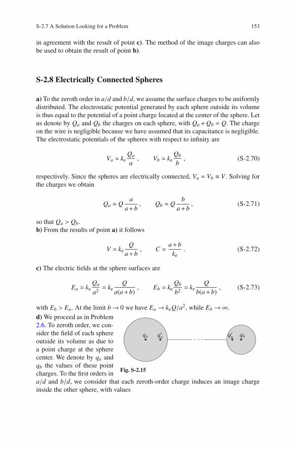
S-2.7 A Solution Looking for a Problem 153
in agreement with the result of point c). The method of the image charges can also
be used to obtain the result of point b).
S-2.8 Electrically Connected Spheres
a) To the zeroth order in a/d and b/d, we assume the surface charges to be uniformly
distributed. The electrostatic potential generated by each sphere outside its volume
is thus equal to the potential of a point charge located at the center of the sphere. Let
us denote by Qa and Qb the charges on each sphere, with Qa +Qb = Q. The charge
on the wire is negligible because we have assumed that its capacitance is negligible.
The electrostatic potentials of the spheres with respect to infinity are
Va ≃ keQa
a, Vb ≃ ke
Qb
b, (S-2.70)
respectively. Since the spheres are electrically connected, Va = Vb ≡ V . Solving for
the charges we obtain
Qa ≃ Qa
a+b, Qb ≃ Q
b
a+b, (S-2.71)
so that Qa > Qb.
b) From the results of point a) it follows
V ≃ keQ
a+b, C ≃ a+b
ke. (S-2.72)
c) The electric fields at the sphere surfaces are
Ea ≃ keQa
a2= ke
Q
a(a+b), Eb ≃ ke
Qb
b2= ke
Q
b(a+b), (S-2.73)
with Eb > Ea. At the limit b→ 0 we have Ea→ keQ/a2, while Eb→∞.
qbqaqa qb
Fig. S-2.15
d) We proceed as in Problem
2.6. To zeroth order, we con-
sider the field of each sphere
outside its volume as due to
a point charge at the sphere
center. We denote by qa and
qb the values of these point
charges. To the first orders in
a/d and b/d, we consider that each zeroth-order charge induces an image charge
inside the other sphere, with values
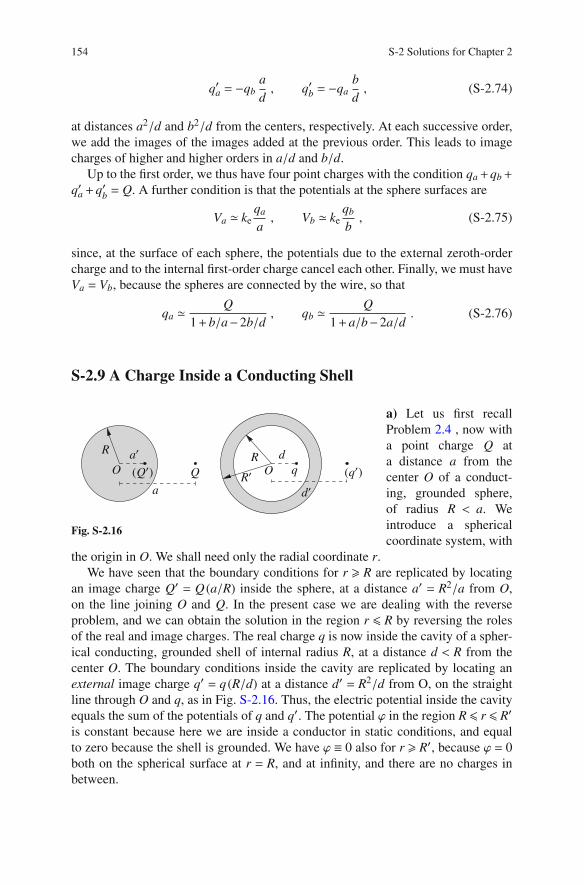
154 S-2 Solutions for Chapter 2
q′a = −qb
a
d, q′b = −qa
b
d, (S-2.74)
at distances a2/d and b2/d from the centers, respectively. At each successive order,
we add the images of the images added at the previous order. This leads to image
charges of higher and higher orders in a/d and b/d.
Up to the first order, we thus have four point charges with the condition qa+qb+
q′a+q′b= Q. A further condition is that the potentials at the sphere surfaces are
Va ≃ keqa
a, Vb ≃ ke
qb
b, (S-2.75)
since, at the surface of each sphere, the potentials due to the external zeroth-order
charge and to the internal first-order charge cancel each other. Finally, we must have
Va = Vb, because the spheres are connected by the wire, so that
qa ≃Q
1+b/a−2b/d, qb ≃
Q
1+a/b−2a/d. (S-2.76)
S-2.9 A Charge Inside a Conducting Shell
a
q(Q )
d
Q (q )
RR
OR
O
da
Fig. S-2.16
a) Let us first recall
Problem 2.4 , now with
a point charge Q at
a distance a from the
center O of a conduct-
ing, grounded sphere,
of radius R < a. We
introduce a spherical
coordinate system, with
the origin in O. We shall need only the radial coordinate r.
We have seen that the boundary conditions for r R are replicated by locating
an image charge Q′ = Q (a/R) inside the sphere, at a distance a′ = R2/a from O,
on the line joining O and Q. In the present case we are dealing with the reverse
problem, and we can obtain the solution in the region r R by reversing the roles
of the real and image charges. The real charge q is now inside the cavity of a spher-
ical conducting, grounded shell of internal radius R, at a distance d < R from the
center O. The boundary conditions inside the cavity are replicated by locating an
external image charge q′ = q (R/d) at a distance d′ = R2/d from O, on the straight
line through O and q, as in Fig. S-2.16. Thus, the electric potential inside the cavity
equals the sum of the potentials of q and q′. The potential ϕ in the region R r R′
is constant because here we are inside a conductor in static conditions, and equal
to zero because the shell is grounded. We have ϕ ≡ 0 also for r R′, because ϕ = 0
both on the spherical surface at r = R, and at infinity, and there are no charges in
between.

S-2.9 A Charge Inside a Conducting Shell 155
b) The force between q and the shell equals the Coulomb force between q and its
image charge q′, and is attractive
F = keqq′
(d′−d)2= −ke
q2Rd
(R2−d2)2. (S-2.77)
c) Let us consider a spherical surface of radius R′′, centered in O, with R < R′′ < R′.The flux of the electric field through this closed surface is zero, because the field
is zero everywhere inside a conductor. The total charge inside the sphere must thus
be zero according to Gauss’s law. This implies that the charge induced on the inner
surface of the shell is −q, as may be verified directly by calculating the surface
charge and integrating over the whole surface.
d) The electric potential must still be constant for R r R′, but it is no longer
constrained to be zero. The electric potential in the region r R is still equivalent to
the potential generated by the charges q and q′ of point a), plus a constant quantity
ϕ0 to be determined. The electric field in the region R r R′ is still zero, so that
the potential is constant and equal to ϕ0. Since the total charge on the shell must
be zero, we must distribute a charge q over its external surface, of radius R′, to
compensate the charge −q distributed over the internal surface, of radius R. Since
the real charge q, and the charge −q distributed over the surface of radius R generate
a constant potential for r R, the charge q must be distributed uniformly over the
external surface in order to keep the total potential constant in the region R r R′.The potential in the region r R′ is equivalent to the potential generated by a
point charge q located in O. Thus we have ϕ(r) = keq/r for r R′, if we choose
ϕ(∞) = 0. Thus ϕ0 = ϕ(R′) = keq/R′, and ϕ(r) = ϕ0 for R r R′. For r R we
have
ϕ(r) = ke
(
q
rq
+q′
rq′
)
+ϕ0, (S-2.78)
where rq is the distance of the point from the real charge q, and rq′ is the distance
of the point from the image charge q′. The field inside the cavity is the same for a
grounded or for an isolated shell.
S-2.10 A Charged Wire in Front of a Cylindrical Conductor
a) We have r =√
(x+a)2+ y2 and r′ =√
(x−a)2+ y2, x and y being the coordinates
of Q. Thus, squaring the equation r/r′ = K we get

156 S-2 Solutions for Chapter 2
(x+a)2+ y2
(x−a)2+ y2= K2
x2+2ax+a2 + y2 = K2x2−2K2ax+K2a2+K2y2
−(x2+ y2)(K2−1)+2ax(K2+1) = a2(K2−1)
x2+ y2−2K2+1
K2−1ax = a2 . (S-2.79)
On the other hand, the equation of a circumference centered at (x0,0) and radius R
is
(x− x0)2+ y2 = R2
x2+ y2−2x0x = R2− x20 . (S-2.80)
Comparing (S-2.80) to (S-2.79) we see that the curves defined by the equation r/r′ =K are circumferences centered at
x0(K) =K2+1
K2−1a , y0 = 0 , (S-2.81)
of radius
R(K) =2K
|K2−1|a . (S-2.82)
Note that
x0
(
1
K
)
= −x0(K) , and R
(
1
K
)
= R(K) . (S-2.83)
Thus, we may restrict ourselves to K > 1, so that x0(K) > a > 0, and omit the
absolute-value sign in the expression for R(K). The circumferences corresponding
to 0 < K < 1 are obtained by reflection across the y axis of the circumferences cor-
responding to 1/K.
b) According to Gauss’s law, the electrostatic field and potential generated by an
infinite straight wire with linear charge density λ are
E(r) =λ
2πε0rand ϕ(r) = − λ
2πε0ln
(
r
r0
)
, (S-2.84)
where r is the distance from the wire and r0 an arbitrary constant, corresponding to
the distance at which we pose ϕ = 0. The potential generated by two parallel wires
of charge densities λ and −λ, respectively, is
ϕ = − λ2πε0
ln
(
r
r0
)
+λ
2πε0ln
(
r′
r′0
)
=λ
2πε0ln
(
r′
r
)
+λ
2πε0ln
(
r0
r′0
)
, (S-2.85)
where r′0
is a second arbitrary constant, analogous to r0. The term
λ
2πε0ln
(
r0
r′0
)
(S-2.86)

S-2.10 A Charged Wire in Front of a Cylindrical Conductor 157
is actually a single arbitrary constant, which we can set equal to zero. With this
choice the electrostatic potential is zero on the x = 0 plane of a Cartesian reference
frame where the two wires lie on the straight lines (x =−a,y= 0) and (x =+a,y= 0).
The equation for the equipotential surfaces in this reference frame is
λ
2πε0ln
(
r′
r
)
= ϕ, (S-2.87)
which leads tor
r′= e−2πε0ϕ/λ . (S-2.88)
Thus we can substitute K = e−2πε0ϕ/λ into (S-2.81) and (S-2.82). We see that the
equipotential surfaces are infinite cylindrical surfaces whose axes have the equations
x0(ϕ) =e−4πε0ϕ/λ+1
e−4πε0ϕ/λ−1, y0 = 0 , (S-2.89)
and their radii are
R(ϕ) =2e−2πε0ϕ/λ
|e−4πε0ϕ/λ−1|a . (S-2.90)
By multiplying the numerators and denominators of the above expressions by
e2πε0ϕ/λ we finally obtain
x0(ϕ) =e−2πε0ϕ/λ+ e2πε0ϕ/λ
e−2πε0ϕλ− e2πε0ϕ/λa = −a coth
(
2πε0ϕ
λ
)
(S-2.91)
and
R(ϕ) =2
|e−2πε0ϕ/λ− e2πε0ϕ/λ|a =
∣
∣
∣
∣
∣
a
sinh(2πε0ϕ/λ)
∣
∣
∣
∣
∣
. (S-2.92)
R
λ
d
d
λ
Fig. S-2.17
If the negative wire is located on the (x = −a,y =
0) straight line, the ϕ > 0 equipotential cylinders are
located in the x< 0 half space (r < r′ in Fig. 2.8), and
the ϕ < 0 equipotentials in the x > 0 half space.
c) We can solve the problem by locating an image
wire with charge density λ′ = −λ inside the cylinder.
In Fig. (2.8), let the real wire intersect the xy plane
at P ≡ (−a,0), and the image wire at P′ ≡ (a,0). The
surface of the conducting cylinder intersects the xy
plane on one of the circumferences r/r′ = K. This is
always possible as far as d > R. With these locations
of the real and image wires the potential of the cylin-
der surface is constant and equal to a certain value ϕ0. Given R and d, we can find
the values of a and d′ by first defining the dimensionless constant ϕ′ = 2πε0ϕ0/λ,
and then solving the simultaneous equations

158 S-2 Solutions for Chapter 2
2a+d′ = d , a+d′ = x0 = acothϕ′ ,a
sinhϕ′= R . (S-2.93)
From the first equation we obtain a = (d−d′)/2, which we substitute into the other
two equationsd+d′
2=
d−d′
2cothϕ′ ,
d−d′
2= Rsinhϕ′ , (S-2.94)
and the latter equation leads to
sinhϕ′ =d−d′
2R, (S-2.95)
independent of λ. From the relations
cosh2 x− sinh2 x = 1 , and coth x =cosh x
sinh x,
we obtain
cothϕ′ =
√
4R2+ (d−d′)2
d−d′, (S-2.96)
which, substituted into the first of (S-2.93) leads to
d+d′
2=
d−d′
2
√
4R2+ (d−d′)2
d−d′. (S-2.97)
Disregarding the trivial solution d′ = d (corresponding to two superposed wires of
linear charge density λ and −λ, generating zero field in the whole space), we have
d′ =R2
d, a =
d2+R2
2d, ϕ′ = arccosh
(
d2+3R2
d2+R2
)
. (S-2.98)
Alternatively, may proceed analogously to the well-known problem of the poten-
tial of a point charge in front of a grounded, conducting sphere.
R
P
r
d
O
d
λ λ
θr
Fig. S-2.18
Figure S-2.18 shows the intersection with
the xy plane of the conducting cylinder of
radius R, the real charged wire at distance
d from the cylinder axis, and the image
wire at distance d′ from the axis. We have
translational symmetry perpendicularly to the
figure. The potential ϕ generated by the real
wire of linear charge density λ, and by the
image wire of linear of linear charge density
λ′ must be constant over the cylinder surface.
The potential at a generic point P of the surface is
ϕ = − λ2πε0
lnr− λ′
2πε0lnr′ = const (S-2.99)

S-2.10 A Charged Wire in Front of a Cylindrical Conductor 159
where r is the distance of P from the real wire and r′ the distance of P from the
image wire. Multiplying by −2πε0 we obtain
λ lnr+λ lnr′ = const , (S-2.100)
which can be rewritten by expressing r and r′ in terms of d, d′, R and the angle θ
between r and the radius joining P to the intersection of the cylinder axis with the
xy plane, O, and applying the law of cosines,
λ ln
(
√
d2+R2−2Rd cosθ
)
+λ′ ln(
√
d′2+R2−2Rd′ cosθ
)
= const . (S-2.101)
Differentiating with respect to θ we obtain
λRd sinθ
d2+R2−2Rd cosθ= − λ′Rd′ sinθ
d′2+R2−2Rd′ cosθ, (S-2.102)
implying that λ and λ′ must have opposite signs. Dividing both sides by Rsinθ we
obtain, after some algebra,
λd(
d′2+R2−2Rd′ cosθ)
= −λ′d′(
d2+R2−2Rd cosθ)
λ(
dd′2+dR2−2Rdd′ cosθ)
= −λ′(
d′d2+d′R2−2Rdd′ cosθ)
, (S-2.103)
which requires λ′ = −λ in order to make the equation independent of θ, and, disre-
garding the trivial solution d′ = d, we finally obtain
d′ =R2
d. (S-2.104)
S-2.11 Hemispherical Conducting Surfaces
O
q
a
q1
q2
R
q3
θθ
φ
z
r
a
Fig. S-2.19
a) We choose a cylindrical coordinate system (r,φ,z)
with the symmetry axis of the problem as z axis, so
that the point charge is located in (asinθ,φ,acosθ),
with φ a given fixed angle, as in Fig. S-2.19. The con-
ductor surface, comprising the hemispherical boss
and the plane part, is equipotential with ϕ = 0. If
the conductor surface were simply plane, with no
boss, the problem would be solved by locating an
image charge q1 = −q in (asinθ,φ,−acosθ), as in
Fig. S-2.19. On the other hand, if the conductor were
a grounded spherical surface of radius R, the prob-
lem would be solved by locating an image charge
q2 = −q(R/a) in (a′ sinθ,φ,a′ cosθ), with a′ = R2/a.
The real charge q, with the two image charges q1 and q2, gives origin to a potential

160 S-2 Solutions for Chapter 2
ϕ(r) = ϕq(r)+ϕq1(r)+ϕq2
(r) which is different from zero both on the plane surface,
where it equals ϕq2(r), since ϕq(r)+ϕq1
(r) = 0 on the plane, and on the hemispher-
ical surface, where it equals ϕq1(r). The problem is solved by adding a third image
charge q3 = q(R/a) at (a′ sinθ,φ,−a′ cosθ), so that the pairs q,q1 and q2,q3 gener-
ate a potential ϕ = 0 on the plane surface, and the pairs q,q2 and q1,q3 generate a
potential ϕ = 0 on the spherical (and hemispherical!) surface. According to Gauss’s
law, the total charge induced on the conductor equals the sum of the image charges
qind = q1+q2+q3 = −q+
(
−R
aq
)
+
(
R
aq
)
= −q . (S-2.105)
O
q2q3
q
R
q1
R2 / b
θθb
Fig. S-2.20
Note that, since the electric field generated by the
real charge plus the three image charges is always
perpendicular to the conductor surface, it must be
zero on the circumference (R,φ,0), here with φ any,
where the hemisphere joins the plane.
b) Now the real charge q is located at (bsinθ,φ,
bcosθ) inside the hemispherical cavity of radius R >
b in the conductor, as in Fig. S-2.20. The solution is
analogous to the solution of point a): we locate three
image charges in the conductor, outside of the cavity,
namely, q1 = −q in (bsinθ,φ,−bcosθ), q2 = −(R/b)q
in (b′ sinθ,φ,b′ cosθ), with b′ = R2/b > R, and q3 =
−q2 = (R/b)q in (b′ sinθ,φ,−b′ cosθ).
S-2.12 The Force between the Plates of a Capacitor
h
+
−σ
σ
E
S
Fig. S-2.21
We present this simple problem in order to point
out, and prevent, two typical recurrent errors. The
first error regards the electrostatic pressure at the
surface of a conductor, the second the derivation
of the force from the energy of a system.
a) Let us consider the electrostatic pressure first.
If Q is the charge of the capacitor, and S the
surface of its plates, the surface charge density
(which is located on the inner surfaces only!)
is ±σ = ±Q/S . Within our approximations, the
electric field is uniform between the two charged
surfaces, E = 4πkeσ, and zero everywhere else.
This leads to an electrostatic pressure
P =1
2σE = 2πkeσ
2 . (S-2.106)

S-2.12 The Force between the Plates of a Capacitor 161
Here, the typical mistake is to forget the 1/2 factor and to write Pw= σE (the “w” on
the “=” sign stands for wrong!). In fact, only one half of the electric field is due to
the charge on the other plate. The force F is attractive because the two plates have
opposite charges, and we can write
F = −PS = −2πkeQ2
S 2S = −2πke
Q2
S. (S-2.107)
Thus the force depends on Q only, and is independent of the distance h between the
plates. (S-2.107) is valid both for an isolated capacitor, and for a capacitor connected
to a voltage source maintaining a fixed potential difference V . But, in the latter case,
the charge is no longer constant, and it is convenient to replace Q by the product
CV , remembering that the capacity of a parallel-plate capacitor is C = S/(4πkeh).
Thus
F = −2πke(CV)2
S= − V2S
8πkeh2. (S-2.108)
b) In the case of an isolated capacitor, the force between the plates can also be
evaluated as minus the derivative of the electrostatic energy Ues of the capacitor
with respect to the distance between the plates, h. It is convenient to write Ues as a
function of the charge Q, which is constant for an isolated capacitor,
Ues =Q2
2C= 2πke
Q2h
2S, (S-2.109)
so that the force between the plates is
F = −∂hU es = −2πkeQ2
S, (S-2.110)
in agreement with (S-2.107).
If the capacitor is connected to a voltage source, the potential difference V
between the plates is the constant quantity. Thus, it is more convenient to write
Ues as a function of V
Ues =1
2CV2 =
1
8πke
V2S
h. (S-2.111)
At this point, it is tempting, but wrong, to evaluate the force between the plates as
minus the derivative of Ues with respect to h. We would get
Fw= −∂hUes = +
1
8πke
V2S
h2, (S-2.112)
and, if the “+” sign were correct, now the force would be repulsive, although
equal in magnitude to (S-2.108)! Of course, this cannot be true, since the plates have
opposite charges and attract each other. The error is that the force equals minus the
gradient of the potential energy of an isolated system, which now includes also the

162 S-2 Solutions for Chapter 2
voltage source. And the voltage source has to do some work to keep the potential dif-
ference of the capacitor constant while the capacity is changing. Let us consider an
infinitesimal variation of the plate separation, dh which leads to an infinitesimal vari-
ation of the capacity, dC. The voltage source must move a charge dQ = VdC across
the potential difference V , in order to keep V constant. The source thus does a work
dW = VdQ = V2dC , (S-2.113)
and its internal energy (whatever its nature: mechanical, chemical, . . . ) must change
by the amount
dUsource = −dW = −V2dC . (S-2.114)
Since at the same time the electrostatic energy of the capacitor changes by 1/2 V2dC,
the variation of the total energy of the isolated system, dUtot, is
dUtot = dUsource+dUes = −V2dC+V2
2dC = −V2
2dC = −dUes . (S-2.115)
Thus, the force is
F = −∂hUtot = +∂hUes = −V2S
8πkeh2, (S-2.116)
in agreement with (S-2.108).
S-2.13 Electrostatic Pressure on a Conducting Sphere
a) The surface charge is σ = Q/S , where S = 4πa2 is the surface of the sphere. The
electric field at the surface is E = 4πkeσ, so that the pressure is
P =1
2σE = 2πkeσ
2 = keQ2
8πa4. (S-2.117)
b) According to Gauss’s law, the electric field of the sphere is
E(r) =
⎧
⎪
⎪
⎪
⎨
⎪
⎪
⎪
⎩
0 , r < a ,
keQ
r2, r > a ,
(S-2.118)
and thus the electrostatic energy is
Ues =
∫
1
8πkeE2(r)d3r =
∫ ∞
a
ke
8π
(
Q
r2
)2
4πr2 dr = keQ2
2a. (S-2.119)
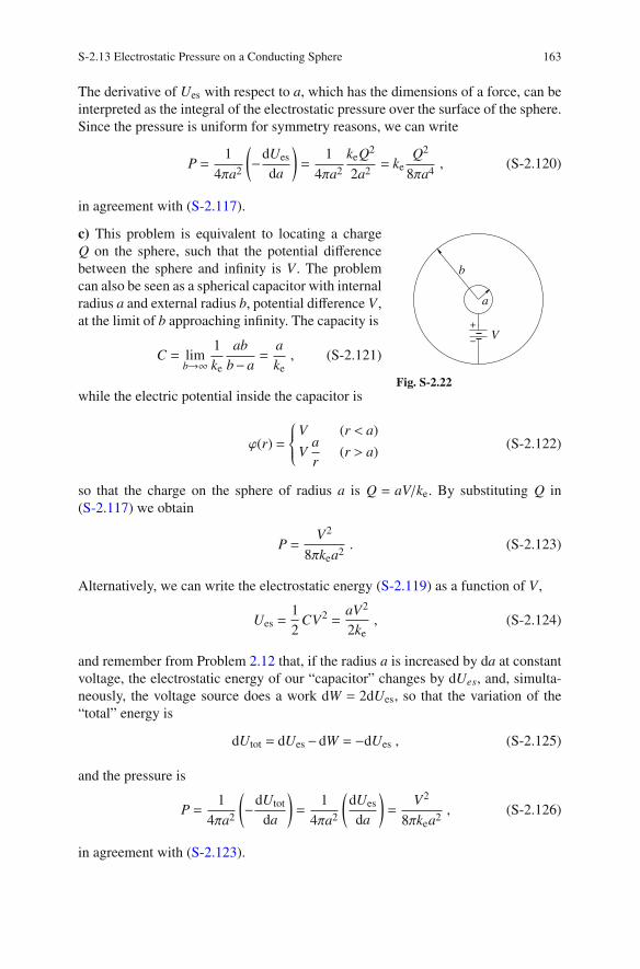
S-2.13 Electrostatic Pressure on a Conducting Sphere 163
The derivative of Ues with respect to a, which has the dimensions of a force, can be
interpreted as the integral of the electrostatic pressure over the surface of the sphere.
Since the pressure is uniform for symmetry reasons, we can write
P =1
4πa2
(
−dUes
da
)
=1
4πa2
keQ2
2a2= ke
Q2
8πa4, (S-2.120)
in agreement with (S-2.117).
−
+V
b
a
Fig. S-2.22
c) This problem is equivalent to locating a charge
Q on the sphere, such that the potential difference
between the sphere and infinity is V . The problem
can also be seen as a spherical capacitor with internal
radius a and external radius b, potential difference V ,
at the limit of b approaching infinity. The capacity is
C = limb→∞
1
ke
ab
b−a=
a
ke, (S-2.121)
while the electric potential inside the capacitor is
ϕ(r) =
⎧
⎪
⎪
⎨
⎪
⎪
⎩
V (r < a)
Va
r(r > a)
(S-2.122)
so that the charge on the sphere of radius a is Q = aV/ke. By substituting Q in
(S-2.117) we obtain
P =V2
8πkea2. (S-2.123)
Alternatively, we can write the electrostatic energy (S-2.119) as a function of V ,
Ues =1
2CV2 =
aV2
2ke, (S-2.124)
and remember from Problem 2.12 that, if the radius a is increased by da at constant
voltage, the electrostatic energy of our “capacitor” changes by dUes, and, simulta-
neously, the voltage source does a work dW = 2dUes, so that the variation of the
“total” energy is
dUtot = dUes−dW = −dUes , (S-2.125)
and the pressure is
P =1
4πa2
(
−dUtot
da
)
=1
4πa2
(
dUes
da
)
=V2
8πkea2, (S-2.126)
in agreement with (S-2.123).
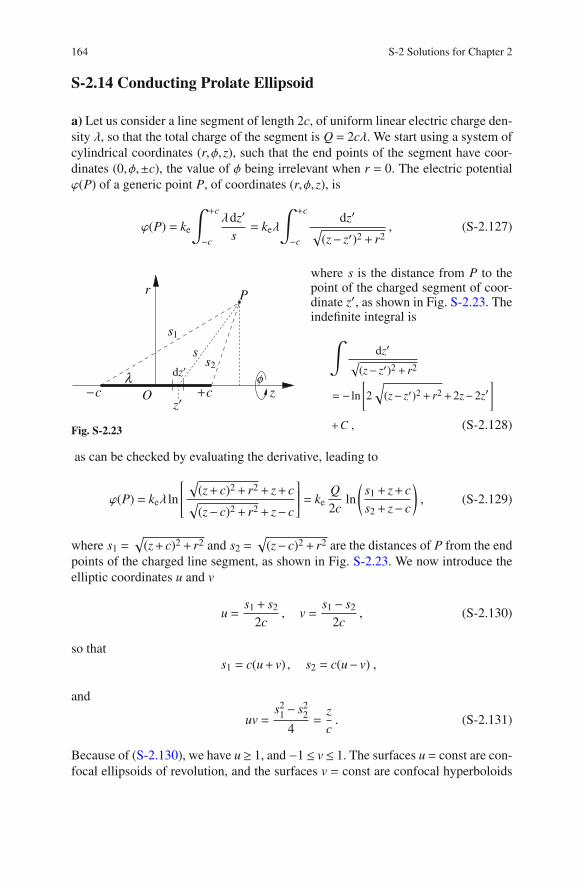
164 S-2 Solutions for Chapter 2
S-2.14 Conducting Prolate Ellipsoid
a) Let us consider a line segment of length 2c, of uniform linear electric charge den-
sity λ, so that the total charge of the segment is Q = 2cλ. We start using a system of
cylindrical coordinates (r,φ,z), such that the end points of the segment have coor-
dinates (0,φ,±c), the value of φ being irrelevant when r = 0. The electric potential
ϕ(P) of a generic point P, of coordinates (r,φ,z), is
ϕ(P) = ke
∫
+c
−c
λdz′
s= keλ
∫
+c
−c
dz′√
(z− z′)2+ r2, (S-2.127)
z
r P
λO
φdz
z
s2
s1
s
−c +c
Fig. S-2.23
where s is the distance from P to thepoint of the charged segment of coor-dinate z′, as shown in Fig. S-2.23. Theindefinite integral is
∫
dz′√
(z− z′)2 + r2
= − ln
[
2
√
(z− z′)2 + r2 +2z−2z′]
+C , (S-2.128)
as can be checked by evaluating the derivative, leading to
ϕ(P) = keλ ln
⎡
⎢
⎢
⎢
⎢
⎢
⎣
√
(z+ c)2+ r2+ z+ c√
(z− c)2+ r2+ z− c
⎤
⎥
⎥
⎥
⎥
⎥
⎦
= keQ
2cln
(
s1+ z+ c
s2+ z− c
)
, (S-2.129)
where s1 =√
(z+ c)2+ r2 and s2 =√
(z− c)2+ r2 are the distances of P from the end
points of the charged line segment, as shown in Fig. S-2.23. We now introduce the
elliptic coordinates u and v
u =s1+ s2
2c, v =
s1− s2
2c, (S-2.130)
so that
s1 = c(u+ v) , s2 = c(u− v) ,
and
uv =s2
1− s2
2
4=
z
c. (S-2.131)
Because of (S-2.130), we have u≥ 1, and −1≤ v≤ 1. The surfaces u= const are con-
focal ellipsoids of revolution, and the surfaces v = const are confocal hyperboloids
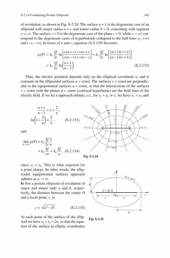
S-2.14 Conducting Prolate Ellipsoid 165
of revolution, as shown in Fig. S-2.24. The surface u = 1 is the degenerate case of an
ellipsoid with major radius a = c and minor radius b = 0, coinciding with segment
(−c,c). The surface v = 0 is the degenerate case of the plane z = 0, while v = ±1 cor-
respond to the degenerate cases of hyperboloids collapsed to the half-lines (c,+∞)
and (−c,−∞). In terms of u and v, equation (S-2.129) becomes
ϕ(P) = keQ
2cln
[
c(u+ v)+ cuv+ c
c(u− v)+ cuv− c
]
= keQ
2cln
[
(u+1)(v+1)
(u−1)(v+1)
]
= keQ
2cln
(
u+1
u−1
)
, (S-2.132)
Thus, the electric potential depends only on the elliptical coordinate u, and is
constant on the ellipsoidal surfaces u = const. The surfaces v = const are perpendic-
ular to the equipotential surfaces u = const, so that the intersections of the surfaces
v = const with the planes φ = const (confocal hyperbolae) are the field lines of the
electric field. If we let u approach infinity, i.e., for s1+ s2≫ c, we have s1 ≃ s2 and
= −1
= 0.92
=0.
707
= 1
=0.3
83
u = 1.667
u = 1.333
c−c
u = 1.033
=−0.707
=0
= −0.92
=−
0.383
Fig. S-2.24
u+1
u−1≃ 1+
2
u,
ln
(
1+2
u
)
≃ 2
u, (S-2.133)
and
limu→∞ϕ(P) = ke
Q
2c
2
u
= keQ
cu≃ ke
Q
s1, (S-2.134)
a
b
czO
c
ru = a/ c
λ = Q/ 2c
Fig. S-2.25
since s1 ≃ s2. This is what expected for
a point charge. In other words, the ellip-
soidal equipotential surfaces approach
spheres as u→∞.
b) For a prolate ellipsoid of revolution of
major and minor radii a and b, respec-
tively, the distance between the center O
and a focal point, c, is
c =√
a2−b2 . (S-2.135)
At each point of the surface of the ellip-
soid we have s1+ s2 = 2a, so that the equa-
tion of the surface in elliptic coordinates

166 S-2 Solutions for Chapter 2
is u = a/c. A uniformly charged line segment with end points at (0,φ,−c) and
(0,φ,c), and linear charge density λ = Q/(2c), generates a constant electric potential
ϕ(a,b) on the surface of the ellipsoid
ϕ(a,b) = keQ
2cln
(
u+1
u−1
)
= keQ
2√
a2−b2ln
⎛
⎜
⎜
⎜
⎜
⎜
⎝
a+√
a2−b2
a−√
a2−b2
⎞
⎟
⎟
⎟
⎟
⎟
⎠
. (S-2.136)
On the other hand, the potential generated by the charged segment at infinity is zero,
and there are no charges between the surface of the ellipsoid and infinity. The flux
of the electric field through any closed surface containing the ellipsoid is Q. Thus,
the potential, and the electric field, generated by the charged segment outside the
surface of the ellipsoid equal the potential, and the electric field, generated by the
conducting ellipsoid carrying a charge Q, and this solves the problem. The capacity
of the ellipsoid is thus
C =Q
ϕ(a,b)=
2√
a2−b2
ke
⎡
⎢
⎢
⎢
⎢
⎢
⎣
ln
⎛
⎜
⎜
⎜
⎜
⎜
⎝
a+√
a2−b2
a−√
a2−b2
⎞
⎟
⎟
⎟
⎟
⎟
⎠
⎤
⎥
⎥
⎥
⎥
⎥
⎦
−1
. (S-2.137)
The denominator of the argument of the logarithm can be rationalized, leading to
a+√
a2−b2
a−√
a2−b2=
(
a+√
a2−b2)2
a−a2+b2=
⎛
⎜
⎜
⎜
⎜
⎜
⎝
a+√
a2−b2
b,
⎞
⎟
⎟
⎟
⎟
⎟
⎠
2
(S-2.138)
and the capacity of the prolate ellipsoid can be rewritten
C =
√a2−b2
ke
⎡
⎢
⎢
⎢
⎢
⎢
⎣
ln
⎛
⎜
⎜
⎜
⎜
⎜
⎝
a+√
a2−b2
b
⎞
⎟
⎟
⎟
⎟
⎟
⎠
⎤
⎥
⎥
⎥
⎥
⎥
⎦
−1
. (S-2.139)
The plates of a confocal ellipsoidal capacitor are the surfaces of two prolate ellip-
soids of revolution, sharing the same focal points located at ±c on the z axis, and
of major radii a1 and a2, respectively, with a1 < a2. According to (S-2.135) and
(S-2.136) the potential on the two plates are
ϕ1,2 = keQ
2cln
(
a1,2+ c
a1,2− c
)
(S-2.140)
so that the capacity is
C =Q
ϕ1−ϕ2=
2c
ke ln
(
a1+ c
a1− c
a2− c
a2+ c
) =2c
ke ln
(
a1a2− c2+ c (a2−a1)
a1a2− c2− c (a2−a1)
). (S-2.141)

S-2.14 Conducting Prolate Ellipsoid 167
c) A straight wire of length h and diameter 2b, with h≫ b, can be approximated by
an ellipsoid prolate in the extreme, with major radius a = h/2 and minor radius b,
with, of course, b≪ a. From
√
a2−b2 ≃ a− b2
avalid for b≪ a , (S-2.142)
and (S-2.139) we have
Cwire ≃a
2ke ln(2a/b)=
h
ke ln(h/b). (S-2.143)

Chapter S-3
Solutions for Chapter 3
S-3.1 An Artificial Dielectric
a) According to (S-2.6) of Problem 2.1, a metal sphere in a uniform external field E
acquires a dipole moment
p =a3
keE =
3
4πkeV E , (S-3.1)
where V = 4/3 πa3 is the volume of the sphere. The polarization of our suspension
is
P = np =3n
4πkeV E . (S-3.2)
In SI units we have P = ε0χE, and χ = 3 f , while in Gaussian units we have P = χE,
and χ = 3 f /(4π). In both cases f = nV is the fraction of the volume occupied by the
spheres. Since the minimum distance between the centers of two spheres is 2a, we
have
f ≤ 4πa3
3
1
8a3=π
6, (S-3.3)
leading to χ ≤ π/2 in SI units, and χ ≤ 1/8 in Gaussian units.
b) The average distance ℓ between two sphere centers is of the order of n−1/3. The
electric field of a dipole at a distance ℓ is of the order of
Edip ≃ kep
ℓ3≃ ke
a3
keE n = a3E n. (S-3.4)
Thus, the condition Edip≪ E requires n≪ 1/a3.
c© Springer International Publishing AG 2017
A. Macchi et al., Problems in Classical Electromagnetism,
DOI 10.1007/978-3-319-63133-2 16
169

170 S-3 Solutions for Chapter 3
S-3.2 Charge in Front of a Dielectric Half-Space
Fig. S-3.1
We denote by A the z < 0, vacuum, half-space,
containing the real charge q, and by B the z > 0,
dielectric, half-space, containing no free charge.
We shall treat the two half spaces separately,
making educated guesses, in order to apply the
uniqueness theorem for the Poisson equation. We
use cylindrical coordinates (r,φ,z), with the real
charge located at (0,φ,−d). All our formulas will
be independent of the azimuthal coordinate φ,
which is not determined, and not relevant, when
r = 0.
a) We treat the field in the half-space A assuming vacuum in the whole space,
including the half-space B. As ansatz, we locate an image charge q′, of value to
be determined, at (0,0,+d), in the half space that we are not considering, as in Fig.
S-3.1. Now we evaluate the electric field E(−) in a generic point P ≡ (r,φ,0−) of
the plane z = 0−. The distance between P and q is√
d2+ r2 and forms an angle
θ = arccos(d/√
d2+ r2) with the z axis. Also the distance between P and q′ will be√d2+ r2. The field at P, E(−), is the vector sum of the fields E due to the real charge
q, and E′ do to the image charge q′. The components of E(−), perpendicular and
parallel to the z = 0 plane are, respectively
E(−)⊥ = ke
q
d2+ r2cosθ− ke
q′
d2+ r2cosθ = ke
d
(d2+ r2)3/2(q−q′)
E(−)
‖ = keq
d2+ r2sinθ+ ke
q′
d2+ r2sinθ = ke
r
(d2+ r2)3/2(q+q′)
. (S-3.5)
Fig. S-3.2
We treat the half-space B assuming that the
whole space, including the half-space A, is
filled by a dielectric medium of relative per-
mittivity εr. We are not allowed to introduce
charges or alter anything in B, but, as an edu-
cated guess, we replace the real charge q,
located in the half-space A that we are not treat-
ing, by a charge q′′, of value to be determined
(Fig. S-3.2). We evaluate the field E(+) at the
same point P as before, but on the z= 0+ plane.
The components of E(+) perpendicular and par-
allel to the z = 0 plane are
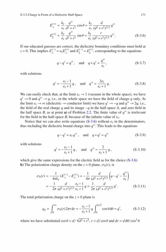
S-3.2 Charge in Front of a Dielectric Half-Space 171
E(+)⊥ =
ke
εr
q′′
d2+ r2cosθ =
ke
εr
d
(d2+ r2)3/2q′′
E(+)
‖ =ke
εr
q′′
d2+ r2sinθ =
ke
εr
r
(d2+ r2)3/2q′′ . (S-3.6)
If our educated guesses are correct, the dielectric boundary conditions must hold at
z = 0. This implies E(−)⊥ = εrE
(+)⊥ and E
(−)
‖ = E(+)
‖ , corresponding to the equations
q−q′ = q′′ , and q+q′ =q′′
εr, (S-3.7)
with solutions
q′ = −εr −1
εr +1q , and q′′ =
2εr
εr+1q . (S-3.8)
We can easily check that, at the limit εr→ 1 (vacuum in the whole space), we have
q′ → 0 and q′′ → q, i.e., in the whole space we have the field of charge q only. At
the limit εr→∞ (dielectric→ conductor limit) we have q′→−q and q′′→ 2q, i.e.,
the field of the real charge q and its image −q in the half-space A, and zero field in
the half space B, as at point a) of Problem 2.2. The finite value of q′′ is irrelevant
for the field in the half-space B, because of the infinite value of εr.
Notice that we can also write equations (S-3.6) without εr in the denominators,
thus including the dielectric bound charge into q′′. This leads to the equations
q−q′ = εr q′′ , and q+q′ = q′′ (S-3.9)
with solutions
q′ = −εr−1
εr+1q , and q′′ =
2
εr+1q , (S-3.10)
which give the same expressions for the electric field as for the choice (S-3.6).
b) The polarization charge density on the z = 0 plane, σb(r), is
σb(r) = − 1
4πke(E
(−)⊥ −E
(+)⊥ ) = − 1
4π
d
(d2+ r2)3/2
(
q−q′− q′′
εr
)
= − 1
2π
d
(d2+ r2)3/2
εr−1
εr+1q =
1
2π
d
(d2+ r2)3/2q′ . (S-3.11)
The total polarization charge on the z = 0 plane is
qp =
∫ ∞
0
σb(r)2πr dr = −εr−1
εr+1q
∫ π/2
0
cosθdθ = q′, (S-3.12)
where we have substituted cosθ = d/√
d2+ r2, r = d/cosθ and dr = d dθ/cos2 θ.

172 S-3 Solutions for Chapter 3
c) The polarization charge of the z = 0 plane generates an electric field equal to the
field of a charge q′ = −q (εr −1)/(εr +1) located at (0,0,+d) in the half space z < 0,
and equal to the field of a charge q′ located at (0,0,−d) in the half space z > 0.
S-3.3 An Electrically Polarized Sphere
a) Since the polarization P of the sphere is uniform, we have no volume bound-
charge density, according to b = ∇ · P. If we choose a spherical coordinate system
(r, θ,φ) with the azimuthal axis parallel to P, as shown in Fig. S-3.3, we see that the
surface bound-charge density of the sphere is σb = Pcosθ, according to σb = P · n.
Thus, in principle, we can evaluate the electric field everywhere in space as the field
generated by the bound-charge distribution on the sphere surface.
However, it is easier to consider the polarized sphere as the superposition of two
uniformly charged spheres, both of radius a, one of volume charge density , and
one of volume charge density −. The centers of the two spheres are separated by a
small distance δ, as in Fig. 1.1 of Problem 1.1. Thus, two initially superposed infini-
tesimal volume elements d3r of the two spheres, of charge ±d3r, respectively, give
origin to an infinitesimal electrical dipole moment dp = δd3r after the displace-
ment.
Fig. S-3.3
This corresponds to a polarization dp/d3r = δ, we
must have P = δ, and are interested in the limit
|δ| → 0, ρ → ∞, with δ = P = constant. Now we
can follow the solution of Problem 1.1. According to
(S-1.1), the electric field inside the sphere is uniform
and equals
Ein = −4πke
3δ = −4πke
3P . (S-3.13)
The problem of the field outside the sphere is solved at point b) of Problem 1.1,
we have
Eext(r) = ke3r (p · r)−p
r3, (S-3.14)
where p = P(4πa3/3) is the total dipole moment of the sphere.
Fig. S-3.4
b) The problem can be solved by the superposition
principle. The hole of radius b can be regarded as a
sphere of uniform electrical polarization −P super-
posed to the sphere of radius a and polarization P.
The sphere of radius b generates a field
E(b)
in=
4πke
3P (S-3.15)

S-3.3 An Electrically Polarized Sphere 173
at its interior. Thus, the total field inside the spherical hole is E(a+b)
in= 0. The field
inside the spherical shell b < r < a is the sum of the uniform field (S-3.13) and the
field generated by an electric dipole of moment p(b) located at the center O, with
p(b) = −4πb3
3P . (S-3.16)
Finally, the external field (r > a) equals the field generated by a single dipole p(a+b)
located in O with
p(a+b) =4π(
a3−b3)
3P . (S-3.17)
S-3.4 Dielectric Sphere in an External Field
a) As an educated guess. Let us assume that the external field induces a uniform
electric polarization P in the sphere. We have seen in Problem 3.3 that a sphere of
uniform
Fig. S-3.5
electric polarization P generates a uniform elec-
tric field Epol = −(4πke/3)P at its interior. The
difference is that in the present case P is not per-
manent but it is induced by the local electric field,
and
P =εr−1
4πkeEdiel , (S-3.18)
where Ediel is the field inside the dielectric
sphere, which is the sum of the external and the induced fields:
Ediel = E0+Epol . (S-3.19)
We thus have
Ediel = E0−4πke
3P = E0−
εr −1
3Ediel , (S-3.20)
which can be solved for Ediel:
Ediel =3
εr+2E0 . (S-3.21)
Since εr > 1, the field inside the dielectric sphere is smaller than E0.
The electric field outside the sphere Eout will be given by the sum of E0 and the
field of a dipole

174 S-3 Solutions for Chapter 3
p =4πa3
3P =
a3
3ke
εr−1
εr+2E0 (S-3.22)
located at the center of the of the sphere. Thus
Eout = E0+ ke3(p · r)r−p
r3= E0+
a3
3ke
εr −1
εr +2[3(E0 · r)r−E0] . (S-3.23)
It is instructive, and useful for the following, to check that the above solution
satisfies the boundary conditions at the surface of the sphere. Let us then restart the
problem by assuming that the field Ediel inside the sphere (r < a) is uniform and
parallel to the external field E0, and that the field Eout outside the sphere (r > a)
is the sum of the external field and that of a dipole p located at the center of the
sphere and also parallel to E0. Thus we can write Ediel = αE0 and p = ηE0, with the
constants α and η to be determined by the boundary conditions at r = a. Choosing
a spherical coordinate system with the origin O at the center of the sphere, and the
polar axis z parallel to E0, we have
Edielr = αE0 cosθ Eout
r = E0 cosθ+ keηE02cosθ
r3
Edielθ = αE0 sinθ Eout
θ = E0 sinθ− keηE0sinθ
r3
Edielφ = 0 Eout
φ = 0 . (S-3.24)
The boundary conditions at the surface of the sphere are εrEdiel⊥ = Eout
⊥ and Ediel‖ =
Eout‖ which yields, in spherical coordinates,
εrEdielr (r = a−) = Eout
r (r = a+) Edielθ (r = a−) = Eout
θ (r = a+) . (S-3.25)
Using (S-3.24) and deleting the common factors we obtain
εrα = 1+2ke
a3η , α = 1− ke
a3η , (S-3.26)
whose solutions for α and η are
α = 3/(εr +2) , η =a3
ke
εr−1
εr−2, (S-3.27)
and we eventually recover (S-3.21) and (S-3.22).
b) We make an educated guess analogous to the one of the previous point, i.e., we
assume that the field inside the cavity, Ecav, is uniform and parallel to Ed, and that
the field in the dielectric medium, Ediel, is the sum of Ed and the field of an electric
dipole pc, located at the center of the cavity and parallel to Ed. Thus we can write
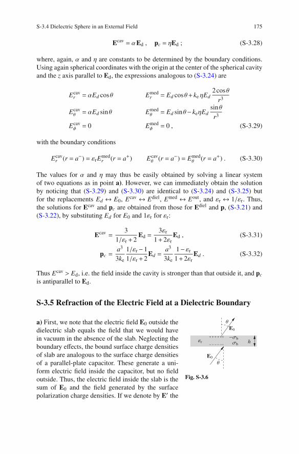
S-3.4 Dielectric Sphere in an External Field 175
Ecav = αEd , pc = ηEd ; (S-3.28)
where, again, α and η are constants to be determined by the boundary conditions.
Using again spherical coordinates with the origin at the center of the spherical cavity
and the z axis parallel to Ed, the expressions analogous to (S-3.24) are
Ecavr = αEd cosθ Emed
r = Ed cosθ+ ke ηEd
2cosθ
r3
Ecavθ = αEd sinθ Emed
θ = Ed sinθ− keηEd
sinθ
r3
Ecavφ = 0 Emed
φ = 0 , (S-3.29)
with the boundary conditions
Ecavr (r = a−) = εrE
medr (r = a+) Ecav
θ (r = a−) = Emedθ (r = a+) . (S-3.30)
The values for α and η may thus be easily obtained by solving a linear system
of two equations as in point a). However, we can immediately obtain the solution
by noticing that (S-3.29) and (S-3.30) are identical to (S-3.24) and (S-3.25) but
for the replacements Ed ↔ E0, Ecav ↔ Ediel, Emed ↔ Eout, and εr ↔ 1/εr. Thus,
the solutions for Ecav and pc are obtained from those for Ediel and p, (S-3.21) and
(S-3.22), by substituting Ed for E0 and 1εr for εr:
Ecav =3
1/εr +2Ed =
3εr
1+2εrEd , (S-3.31)
pc =a3
3ke
1/εr−1
1/εr+2Ed =
a3
3ke
1−εr1+2εr
Ed . (S-3.32)
Thus Ecav > Ed, i.e. the field inside the cavity is stronger than that outside it, and pc
is antiparallel to Ed.
S-3.5 Refraction of the Electric Field at a Dielectric Boundary
Fig. S-3.6
a) First, we note that the electric field E0 outside the
dielectric slab equals the field that we would have
in vacuum in the absence of the slab. Neglecting the
boundary effects, the bound surface charge densities
of slab are analogous to the surface charge densities
of a parallel-plate capacitor. These generate a uni-
form electric field inside the capacitor, but no field
outside. Thus, the electric field inside the slab is the
sum of E0 and the field generated by the surface
polarization charge densities. If we denote by E′ the

176 S-3 Solutions for Chapter 3
internal electric field, the boundary conditions at the dielectric surfaces are
E0⊥ = εr E′⊥ , E0‖ = εr E′‖ , (S-3.33)
where the subscripts ⊥ and ‖ denote the field components perpendicular and parallel
to the interface surface, respectively. In terms of the angles θ and θ′ of Fig. S-3.6
Fig. S-3.7
we have
E0 cosθ = εrE′ cosθ′
E0 sinθ = E′ sinθ′ . (S-3.34)
If we divide the second of (S-3.34) by the first we
obtain
1
εrtanθ′ = tanθ , (S-3.35)
and, since εr > 1, we have θ′ > θ.b) From Gauss’s law we obtain
σb =1
4πke(Eo,⊥−E′⊥) =
1
4πkeE0 cosθ
(
1− 1
εr
)
. (S-3.36)
c) The electrostatic energy density inside the slab is
ues =εr
8πkeE′2 =
εr
8πke, (E′2⊥ +E′2‖ ) =
εr
8πkeE2
0
(
cos2 θ
ε2r+ sin2 θ
)
=1
8πkeεrE2
0
[
(ε2r −1)sin2 θ+1]
, (S-3.37)
so that ues increases with increasing θ, and we expect a torque τ tending to rotate the
slab toward the angle of minimum energy, i.e., θ = 0. Neglecting boundary effects,
the total electrostatic energy of the slab is Ues = Vues, where V is the volume of the
slab, and the torque exerted by the electric field is
τ = −∂Ues
∂θ= − 1
8πkeεrE2
0V(
ε2r −1)
sin2θ < 0 . (S-3.38)

S-3.6 Contact Force between a Conducting Slab and a Dielectric Half-Space 177
S-3.6 Contact Force between a Conducting Slab and a Dielectric
Half-Space
Fig. S-3.8
a) Neglecting boundary effects at the edges of the
slab, the electric field is parallel to the x axis in all
the regions of interest because of symmetry reasons.
Thus, we can omit the vector notation, and we shall
use positive numbers for vectors whose unit vector
is x, negative numbers otherwise.
According to Gauss’s law, a uniformly charged
plane with surface charge density σa generates uni-
form fields at both its sides, of intensities Ea =
±σa/2ε0, respectively. In our problem we have three
charged parallel plane surfaces: we denote by σ1 the
surface charge density on the left surface of the slab,
by σ2 charge the density on its right surface, and by σb the bound surface charge
density of the dielectric material on its surface, as shown in Fig. S-3.8. Since the
total free charge on the slab is Q, we have
σ1+σ2 =Q
S= σtot . (S-3.39)
At any point in space the total electric field is the sum of the fields generated by
the three surface charges. Now, the electric field must be zero inside the conducting
slab. Thus the sum of all surface charge densities (including both free and bound
charges) at the left of the slab must equal the sum of all surface charge densities at
the right, so that their respective fields cancel out inside the slab. This conclusion
holds both when the slab is in contact with the dielectric, and when there is a vacuum
gap between them. Thus, we have
σ1 = σ2+σb . (S-3.40)
The electric field Ed inside the dielectric medium is Ed = 4πke (σ2 + σb). This
implies for the dielectric polarization of the medium P
P =εr −1
4πkeEd = (εr −1)σ1 . (S-3.41)
Since we also have σb = −P · x = −P, we obtain the additional relation
σb = −(εr−1)(σ2+σb) , (S-3.42)
that leads to
σb = −εr−1
εrσ2 . (S-3.43)
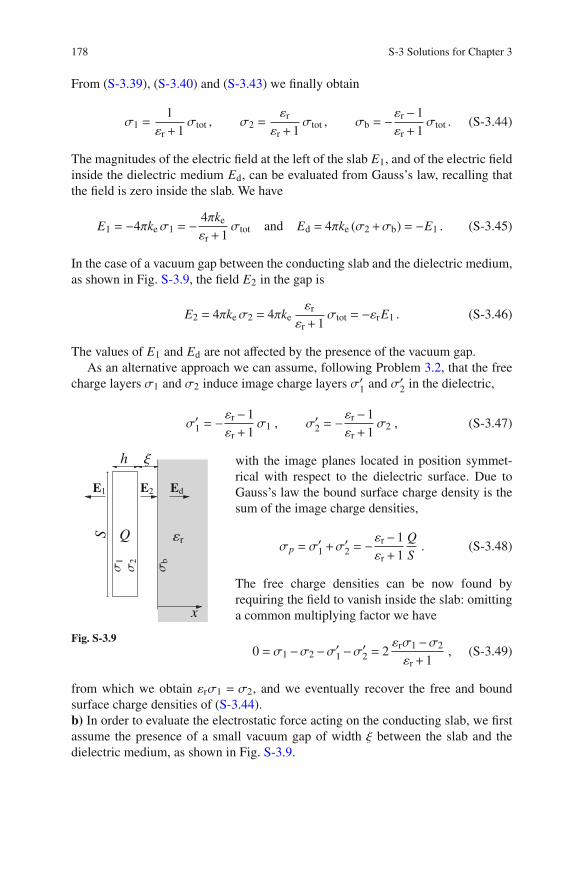
178 S-3 Solutions for Chapter 3
From (S-3.39), (S-3.40) and (S-3.43) we finally obtain
σ1 =1
εr +1σtot , σ2 =
εr
εr+1σtot , σb = −
εr−1
εr+1σtot . (S-3.44)
The magnitudes of the electric field at the left of the slab E1, and of the electric field
inside the dielectric medium Ed, can be evaluated from Gauss’s law, recalling that
the field is zero inside the slab. We have
E1 = −4πkeσ1 = −4πke
εr +1σtot and Ed = 4πke (σ2+σb) = −E1 . (S-3.45)
In the case of a vacuum gap between the conducting slab and the dielectric medium,
as shown in Fig. S-3.9, the field E2 in the gap is
E2 = 4πkeσ2 = 4πkeεr
εr+1σtot = −εrE1 . (S-3.46)
The values of E1 and Ed are not affected by the presence of the vacuum gap.
As an alternative approach we can assume, following Problem 3.2, that the free
charge layers σ1 and σ2 induce image charge layers σ′1
and σ′2
in the dielectric,
σ′1 = −εr−1
εr+1σ1 , σ′2 = −
εr −1
εr +1σ2 , (S-3.47)
Fig. S-3.9
with the image planes located in position symmet-
rical with respect to the dielectric surface. Due to
Gauss’s law the bound surface charge density is the
sum of the image charge densities,
σp = σ′1+σ
′2 = −
εr−1
εr+1
Q
S. (S-3.48)
The free charge densities can be now found by
requiring the field to vanish inside the slab: omitting
a common multiplying factor we have
0 = σ1−σ2−σ′1−σ′2 = 2
εrσ1−σ2
εr+1, (S-3.49)
from which we obtain εrσ1 = σ2, and we eventually recover the free and bound
surface charge densities of (S-3.44).
b) In order to evaluate the electrostatic force acting on the conducting slab, we first
assume the presence of a small vacuum gap of width ξ between the slab and the
dielectric medium, as shown in Fig. S-3.9.

S-3.6 Contact Force between a Conducting Slab and a Dielectric Half-Space 179
We can evaluate the total electrostatic force F acting on the conducting slab in
three equivalent ways:
(i) We can evaluate the variation of the total electrostatic energy Ues when the
slab is displaced by an infinitesimal amount dx toward the right, thus decreas-
ing the gap. In this case Ues increases by E21
S dx/(8πke) at the left of the
slab, because the width of region “filled” by the field E1 increases by dx,
and correspondingly decreases by E22
S dx/(8πke) at its right. Thus, dUes =
(E21−E2
2)S dx/(8πke), from which we obtain the force per unit surface
F = −dUes
dx=
S
8πke(E2
1 −E22) =
S
8πke(ε2r −1)
(
4πke
εr+1
)2 (Q
S
)2
= 2πke
εr−1
εr+1
Q2
S. (S-3.50)
We have F > 0, meaning that the slab is attracted by the dielectric medium.
(ii) We can multiply the charge of the slab Q by the local field, i.e., by the field
generated by all charges excluding the charges of the slab. In our case the local
field is the field Ep generated by the bound surface charge density σb. We have
Ep = −2πkeσb = 2πkeεr −1
εr +1σtot , and F = 2πke
εr −1
εr +1
Q2
S. (S-3.51)
(iii) We can evaluate the force on the slab by summing the forces F1 on its left
and F2 on its right surface. These are obtained by multiplying the respective
charges Q1 = Sσ1 and Q2 = Sσ2 by the average fields at the surfaces
F = F1+F2 = Q1E1
2+Q2
E2
2= − Q
εr+1
2πke
εr+1σtot+
εrQ
εr+1
εr2πke
εr+1σtot
= 2πke
ε2r −1
(εr+1)2
Q2
S= 2πke
εr−1
εr+1
Q2
S. (S-3.52)
The force F is independent of ξ, thus the above result should be valid also at the
limit ξ → 0, i.e., when there is contact between the metal slab and the dielectric.
One may argue, however, that in these conditions the field at x = 0+, i.e., at the right
of the slab, is given by Ed = −E1, so that following the approach (iii) one would
write
F = F1+F2?= Q1
E1
2+Q2
Ed
2 Q1
E1
2+Q2
E2
2. (S-3.53)
This discrepancy comes out because actually the average field on the free charges
located on the right surface of the slab is not Ed/2, which is the average field across
the two merging layers of free and bound charges; however, the force on the slab
must be calculated by taking the average field on free charges only.

180 S-3 Solutions for Chapter 3
Fig. S-3.10
To illustrate this issue, let us assume for a
moment the free charges at the slab surfaces
to be distributed in a layer of small but finite
width, so that we can localize exactly where
free charges are without merging them with
bound charges. In particular, let the free sur-
face charge layer have thickness ℓ2 and vol-
ume charge density 2(x) such that
∫ 0
−ℓ22 dx = σ2 , (S-3.54)
Fig. S-3.11
as shown in Fig. S-3.10. The electric field is
still directed along the x axis for symmetry
reasons. Gauss’s law in one dimension gives
∂xE = 4πke. Since E(−ℓ2) = 0 (as deep into
the conductor the field should vanish) we have
for the electric field in the −ℓ2 x 0 region
E(x) = 4πke
∫ x
−ℓ22(x′)dx′ . (S-3.55)
The total force on the free charges only can
thus be evaluated as
F2 = S
∫ 0
−ℓ2E(x)2(x)dx
=S
4πke
∫ 0
−ℓ2E(x)∂xE(x)dx =
S
8πke
∫ 0
−ℓ2∂xE2(x)dx
=S
8πkeE2
2 =S (4πkeσ2)2
8πke= 2πke Sσ2
2 , (S-3.56)
the electric field at x = 0− is E2, as shown in Fig. S-3.11, and the resulting elec-
trostatic pressure is p2 = F2/S = 2πkeσ22, independent of the particular distribution
2(x), and in agreement with the previous result (S-3.52). However, the electric field
at x = 0+ is Ed because of the presence of the surface bound charge. 1
c) If the dielectric medium is actually a slab limited at x = w, as shown in Fig.
S-3.12, a further bound surface charge density −σb, opposite to the density σb at
x = 0, appears at its x = w surface. This charge distribution is identical to that of
a plane capacitor, so that the bound charges generate no field outside the dielectric
1We might assume that also the polarization charge fills a layer of small, but finite width ℓd at the
surface of the dielectric. However, this would only imply that the field becomes Ed at x ℓd, and
would not affect our conclusions on the forces on the conductor.

S-3.6 Contact Force between a Conducting Slab and a Dielectric Half-Space 181
slab. As trivial consequences the surface charge densities on the conducting slab are
σ1 = −σ2 = Q/2S , the field inside the dielectric is E1/εr = Q/(2ε0εrS ), and there is
no force between the slab and the dielectric. Moreover, this result is independent of
w, and therefore should be valid also in the limit w→∞.
Fig. S-3.12
The apparent contradiction with the results
of points a) and b) is that, in two attempts
to approximate real conditions by objects
of infinite size, we are assuming different
boundary conditions at infinity. To discuss
this issue let us look again at Fig. 3.5, show-
ing the slab of charge Q located in front of a
dielectric hemisphere of radius R. At the limit
R→∞, the field in the dielectric half-space
approaches the field that we would have if
the dielectric medium filled the whole space,
and the surface S had surface charge density
σ′′ = 2εrσ/(εr + 1), see Problem 3.2. Thus,
the field, the polarization, and the polariza-
tion surface charge density all approach zero at the hemispherical surface. Part b)
of Fig. 3.5 is an enlargement of the area enclosed in the dashed rectangle of part
a) of the same figure, and the vanishing charge density on the hemisphere surface
does not contribute to the field in this area, according to the result of Problem 1.11.
This motivates the boundary condition assumed in points a) and b). In contrast, in
point c) the bound surface charge density does not vanish at infinity and generates
a uniform field, which in vacuum cancels out the field generated by the dielectric
surface at x = 0.
S-3.7 A Conducting Sphere between two Dielectrics
a) We use a spherical coordinate system (r, θ,φ) with the origin O at the center of
the sphere, and the zenith direction perpendicular to the plane separating the two
dielectric media, as shown in Fig. S-3.13. The electric field inside the conducting
sphere is zero. The electric field outside the sphere, E(r, θ,φ), is independent of
φ because of the symmetry of our problem. Since the sphere is conducting, the
electric field E(R+, θ,φ) must be perpendicular to its surface, and its only nonzero
component is Er. If we write Maxwell’s equation ∇×E = 0 in spherical coordinates
over the spherical surface r = R+ (see Table A.1 of the Appendix), we see that the
r and θ components of the curl are automatically zero because Eφ = 0, Eθ = 0, and
all derivatives with respect to φ are zero. The condition that also the φ component
of the curl must be zero is
∂θEr = ∂r(rEθ) = Eθ + r∂rEθ . (S-3.57)

182 S-3 Solutions for Chapter 3
Fig. S-3.13
The right-hand side of (S-3.57) is zero
because Eθ(R−) = Eθ(R
+) = 0, implying that
also ∂rEθ(R) = 0. Thus, ∂θEr(R+) = 0, and
Er(R+) does not depend on θ (and, conse-
quently, on the dielectric medium). If we
denote by σtot the sum of the free surface
charge density σf and the bound charge den-
sity σb, the relation
σtot =E(R+, θ,φ)
4πke=
E(R+)
4πke(S-3.58)
shows that σtot is constant over the whole surface of the sphere. Thus the electric
field in the whole space outside the sphere equals the field of a point charge Qtot
located in O, with Qtot = Q+Qb , where Qb is the total polarization (bound) charge:
E(r, θ,φ) = E(r) = 4πkeσtotR2
r2r , r > R , (S-3.59)
since the field depends on r only. The polarization charge densities on the surfaces
of the two dielectrics in contact with the sphere are, respectively,
σb1 = n ·P1 = −εr1−1
4πkeE(R) = −(εr1−1)σtot
σb2 = n ·P2 = −εr2−1
4πkeE(R) = −(εr2−1)σtot (S-3.60)
where the unit vector n points toward the center of the sphere. The free surface
charge densities in the regions in contact with the two dielectrics, σf1 and σf2, are,
respectively,
σf1 = σtot−σb1 = εr1σtot
σf2 = σtot−σb2 = εr2σtot . (S-3.61)
Since 2πR2(σf1+σf2) = Q, we finally obtain
σtot =Q
2πR2(εr1+εr2)E(r) = 2ke
Q
(εr1+εr2)r2r
σf1 =εr1 Q
2πR2(εr1+εr2)σf2 =
εr2 Q
2πR2(εr1+εr2)
σb1 = −(εr1−1) Q
2πR2(εr1+εr2)σb2 = −
(εr2−1) Q
2πR2(εr1+εr2). (S-3.62)

S-3.7 A Conducting Sphere between two Dielectrics 183
Fig. S-3.14
b) The electrostatic pressures on the two
hemispherical surfaces equal the electrostatic
energy densities in the corresponding dielec-
tric media, and are, respectively,
Pfi =2πke
εriσ2
fi =2πke
εri
[
εri Q
2πR2(εr1+εr2)
]2
= keεri Q2
2πR4(εr1+εr2)2(S-3.63)
with i = 1,2. Thus P1 > P2 because εr1 > εr2,
and the pressure pushes the sphere towards the medium of higher permittivity. The
force on the sphere surface element dS = R2 sinθdθdφ is dF = rPfi dS , with i = 1 if
θ > π/2, and i= 2 if θ < π/2. The total force acting on the upper hemisphere (θ < π/2)
is thus
F2 = z
∫ 2π
0
dφ
∫ π/2
0
dθR2 sinθcosθkeεr2 Q2
2π(εr1+εr2)2R4
= zπR2keεr2Q2
2π(εr1+εr2)2R4= zπR2P2 = zke
εr2Q2
2(εr1+εr2)2R2, (S-3.64)
directed upwards, since the force components perpendicular to the z axis cancel out.
Note that F2 simply equals Pf2 times the section of the sphere πR2. The total force
acting on the lower hemisphere (θ > π/2) is, analogously,
F1 = −zkeεr1 Q2
2(εr1+εr2)2R2. (S-3.65)
The total electrostatic force acting on the conducting sphere is thus
Ftot = F1+F2 = −zke(εr1−εr2) Q2
2(εr1+εr2)2 R2. (S-3.66)
If the sphere is at equilibrium when half of its volume is submerged, Ftot plus the
sphere weight must balance Archimedes’ buoyant force
ke(εr1−εr2) Q2
2(εr1+εr2)2 R2= g
2πR3
3(1+2−2) , (S-3.67)

184 S-3 Solutions for Chapter 3
where g is the gravitational acceleration. Thus, at equilibrium, the electric charge on
the sphere must be
Q =
√
4πR5 (εr1+εr2)2 (1+2−2)g
3ke (εr1−εr2). (S-3.68)
S-3.8 Measuring the Dielectric Constant of a Liquid
The partially filled capacitor is equivalent to two capacitors connected in parallel,
one with vacuum between the plates, and the other filled by the dielectric liquid.
The two capacitors have the same internal and external radii, a and b, but different
lengths, ℓ−h and h, respectively. The total capacitance is
C =ℓ−h
2ke ln(b/a)+
εrh
2ke ln(b/a)=ℓ+ (εr−1)h
2ke ln(b/a), (S-3.69)
and the electrostatic energy of the capacitor is
Ues =12
CV2 =ℓ+ (εr−1)h
4ke ln(b/a)V2 . (S-3.70)
If the liquid raises by an amount dh the capacity increases by
dC =(εr−1)dh
2ke ln(b/a), (S-3.71)
and, if the potential difference V across the capacitor plates is kept constant, the
electrostatic energy of the capacitor increases by an amount
dUes =12
V2dC =(εr−1)dh
4ke ln(b/a)V2 . (S-3.72)
Simultaneously the voltage source does a work
dW = VdQ = V2dC =(εr−1)dh
2ke ln(b/a)V2 , (S-3.73)
because the charge of the capacitor must increase by dQ = VdC in order to keep the
potential difference across the plates constant, and this implies moving a charge dQ
from one plate to the other. The energy of the voltage source changes by
dUsource = −(εr−1)dh
2ke ln(b/a)V2 = −2dUes . (S-3.74)

S-3.8 Measuring the Dielectric Constant of a Liquid 185
We must still evaluate the increase in gravitational potential energy of the liquid.
When the liquid raises by dh an infinitesimal annular cylinder of mass dm = π(b2−a2)dh is added at its top, and the gravitational energy increases by
dUg = gπ(b2−a2)hdh . (S-3.75)
The total energy variation is thus
dUtot = dUes+dUsource+dUg = −dUes+dUg
= − (εr−1)dh
4ke ln(b/a)V2+gπ(b2−a2)hdh , (S-3.76)
and the total force is
F = −∂Utot
∂h=
εr−1
4ke ln(b/a)V2−gπ(b2−a2)h . (S-3.77)
At equilibrium we have F = 0, which corresponds to
h =(εr−1)V2
4πke g(a2−b2) ln(b/a)and εr = 1+
4πke g(a2−b2) ln(b/a)
V2h . (S-3.78)
For the electric susceptibility χ, we have in SI units χ = εr −1, and
χ =g (a2−b2) ln(b/a)
ε0V2h , (S-3.79)
while in Gaussian units we have χ = (εr−1)/4π, and
χ =g (a2−b2) ln(b/a)
V2h . (S-3.80)
S-3.9 A Conducting Cylinder in a Dielectric Liquid
a) We choose a cylindrical coordinate system (r,φ,z) with the longitudinal axis z
superposed to the axis of the conducting cylinder, and the origin O at the height
of the boundary surface between the dielectric liquid and the vacuum above it. The
azimuthal angle φ is irrelevant for the present problem. The electric field E(r,φ,z) is
perpendicular to the surface of the cylinder, thus we have E(r,φ,z) ≡ [Er(r,z),0,0].
The field is continuous at the dielectric-vacuum boundary surface, since it is parallel
to it. We thus have Er(r,z) = Er(r), independently of z. Let us denote by σ1 and σ2
the free-charge surface densities on the cylinder lateral surface for z > 0 and z < 0,
respectively. Quantities σ1 and σ2 are related to the electric field at the cylinder

186 S-3 Solutions for Chapter 3
surface, Er(a), to εr and Q by
σ1 =Er(a)
4πke, σ2 =
εrEr(a)
4πke,
Q = 2πa [σ1h+σ2(L−h)] . (S-3.81)
We thus have
Er(a) = Q2ke
a[h+εr(L−h)]
= Q2ke
a[εrL− (εr−1)h]. (S-3.82)
Fig. S-3.15
b) The electric field Er(r) in the region a <
r < b can be evaluated by applying Gauss’s law
to a closed cylindrical surface of radius r and
height ℓ≪ L, coaxial to the conducting cylinder.
Neglecting the boundary effects, the flux of the
electric field through the bases of the Gaussian
surface is zero, and we have
2πr ℓEr(r) = 4πkeQint ,
Er(r) =2keQint
r ℓ, (S-3.83)
where Qtot is the total charge inside the Gaussian
surface, including both free and polarization
charges. If we let r approach a keeping ℓ constant, Qint remains constant and we
have
limr→a
Er =2keQint
aℓ= Er(a) , so that Er(r) = Er(a)
a
r(S-3.84)
and, inserting (S-3.82),
Er(r) =2keQ
r [εrL− (εr−1)h]. (S-3.85)
c) The electrostatic energy of the system is
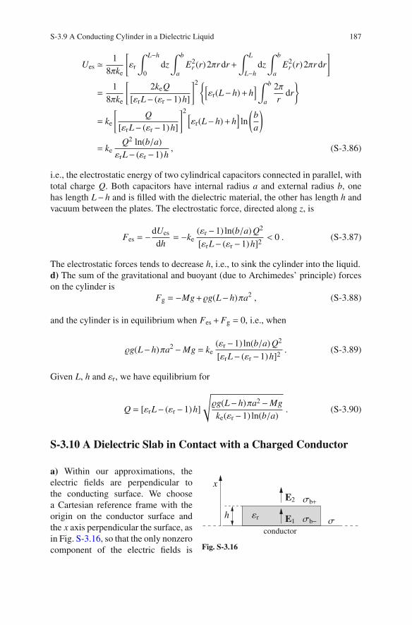
S-3.9 A Conducting Cylinder in a Dielectric Liquid 187
Ues ≃1
8πke
[
εr
∫ L−h
0
dz
∫ b
a
E2r (r)2πr dr+
∫ L
L−h
dz
∫ b
a
E2r (r)2πr dr
]
=1
8πke
[
2keQ
[εrL− (εr−1)h]
]2[
εr(L−h)+h]
∫ b
a
2π
rdr
= ke
[
Q
[εrL− (εr−1)h]
]2[
εr(L−h)+h]
ln
(
b
a
)
= keQ2 ln(b/a)
εrL− (εr−1)h, (S-3.86)
i.e., the electrostatic energy of two cylindrical capacitors connected in parallel, with
total charge Q. Both capacitors have internal radius a and external radius b, one
has length L−h and is filled with the dielectric material, the other has length h and
vacuum between the plates. The electrostatic force, directed along z, is
Fes = −dUes
dh= −ke
(εr−1) ln(b/a) Q2
[εrL− (εr −1)h]2< 0 . (S-3.87)
The electrostatic forces tends to decrease h, i.e., to sink the cylinder into the liquid.
d) The sum of the gravitational and buoyant (due to Archimedes’ principle) forces
on the cylinder is
Fg = −Mg+g(L−h)πa2 , (S-3.88)
and the cylinder is in equilibrium when Fes+Fg = 0, i.e., when
g(L−h)πa2−Mg = ke(εr−1) ln(b/a) Q2
[εrL− (εr −1)h]2. (S-3.89)
Given L, h and εr, we have equilibrium for
Q = [εrL− (εr−1)h]
√
g(L−h)πa2−Mg
ke(εr−1) ln(b/a). (S-3.90)
S-3.10 A Dielectric Slab in Contact with a Charged Conductor
b+
b−
conductor
E2
E1h r
x
Fig. S-3.16
a) Within our approximations, the
electric fields are perpendicular to
the conducting surface. We choose
a Cartesian reference frame with the
origin on the conductor surface and
the x axis perpendicular the surface, as
in Fig. S-3.16, so that the only nonzero
component of the electric fields is

188 S-3 Solutions for Chapter 3
their x component. We denote by E1 the electric field field inside the dielectric
slab, and by E2 the electric field in vacuum, while the field will is zero inside the
conductor.
The fields E1 and E2 can be evaluated by applying equation ∇· (εrE) = 4πke f to
two Gaussian “pillboxes”, crossing the x = 0 and the x = h surfaces, respectively,
b+
b−
conductor
E2
E1h
x
r
Fig. S-3.17
as in Fig. S-3.17. We see that εrE is
discontinuous at x = 0 surface, and
continuous at x = h:
εrE1 = 4πkeσ ,
E2 = εrE1 , (S-3.91)
which lead to
E1 =4πke
εrσ , E2 = 4πkeσ. (S-3.92)
b) We denote by σb− and σb+ the surface polarization charge densities at x = 0
and x = h, respectively. These quantities can be calculated by applying Gauss’s law
∇ ·E = 4πke(f +b) to the two “pillboxes” of Fig. S-3.17, and obtaining
E1 = 4πke(σ+σb−) , E2−E1 = 4πkeσb+ , (S-3.93)
introducing (S-3.91) into (S-3.93) we finally have
σb+ = −σb− =
(
1− 1
εr
)
σ =εr −1
εrσ. (S-3.94)
c) In the vacuum region between the conductor and the dielectric slab the field is
E = 4πkeσ = E2, independent of s. The electric field inside the dielectric slab, and
above the slab, are E1 and E2, respectively, as in the case of s= 0, thus independently
of s.
conductor
h r b−E1
b+
s E2
E2x
Fig. S-3.18
The net electrostatic force on the
slab is zero, independently of s, since
the forces on the upper and lower sur-
faces of the slab are exactly opposite.
Further, if we evaluate the electrosta-
tic energy of the system as the vol-
ume integral of εrE2/(8πke), we see
that also this quantity is independent
of s, within our approximations.

S-3.11 A Transversally Polarized Cylinder 189
S-3.11 A Transversally Polarized Cylinder
We choose a cylindrical coordinate system (r,φ,z), with the cylinder axis as z
axis, and the reference plane (the plane from which the angle φ is measured) parallel
to P. We have translational symmetry along z, so that, mathematically, the problem
is two-dimensional. The surface charge polarization density of the cylinder isσ(φ)=
P · n, where n is the outgoing unit vector perpendicular to the cylinder surface, thus
σ(φ) = Pcosφ . (S-3.95)
Similarly to Problem 1.1, our transversally polarized cylinder can be considered as
φ
++
−−
x
+r
−
O+
O−
Phy z
Fig. S-3.19
the limit for h→ 0 and →∞ of two partially
overlapping cylinders, of volume charge den-
sity ±, respectively. The two cylinder axes
are the straight lines x = ±h/2, both out of
paper in Fig. S-3.19. The product h is con-
stant, and equals the polarization P of the
original cylinder. The electrostatic potential
ϕext± (A), generated by each charged cylinder
at an external point A ≡ (r,φ,z), equals the
potential of an infinite line charge of linear
charge density λ± = ±πa2, located on the
cylinder axis,
ϕext± (A) = ∓2keπa
2 ln
(
r±R±
)
, (S-3.96)
z
++
−−
x
+
−
O+
O−
Ph
A
r−
φ
r+
r
Fig. S-3.20
where
r± ≃ r∓ h
2cosφ (S-3.97)
are the distances of A from the axes of
the two cylinders, see Fig. S-3.20. Quanti-
ties R± are two arbitrary constants, such that
ϕext± (r±,φ,z) = 0 on the cylindrical surfaces
r± = R±. It is convenient to choose R+ = R−,
so that ln(R+/R−) = 0 will cancel out in the
following computations, leaving the poten-
tial equal to zero at r = ∞. The electrostatic
potential generated by both cylinders is thus

190 S-3 Solutions for Chapter 3
ϕext(A) = ϕext+ (A)+ϕext
− (A) = 2keπa2 ln
(
r−r+
)
+2keπa2 ln
(
R+
R−
)
≃ 2keπa2 ln
[
r+ (h/2)cosφ
r− (h/2)cosφ
]
= 2keπa2 ln
[
1+ (h/2r)cosφ
1− (h/2r)cosφ
]
= 2keπa2
[
ln
(
1+h
2rcosφ
)
− ln
(
1− h
2rcosφ
)]
≃ 2keπa2
h
rcosφ = 2keπa
2 Pcosφ
r= 2keπa
2 P · rr, (S-3.98)
where r is the unit vector of the cylindrical coordinate r. Thus, the potential of our
two-dimensional electric dipole decreases as r−1, while the potential of the ordinary
electric dipole decreases as r−2. In Cartesian coordinates we have
ϕext(x,y,z) = 2keπa2 Px
x2+ y2, (S-3.99)
where the x and y axes are the ones shown in Fig. S-3.19.
The external electric field is obtained by evaluating Eext =−∇ϕext. The cylindrical
components are, from Table A.1 of the Appendix,
Eextr = −∂rϕ
ext = 2keπa2 Pcosφ
r2,
Eextφ = −
1
r∂φϕ
ext = 2keπa2 Psinφ
r2,
Eextz = −∂zϕ
ext = 0 , (S-3.100)
the field decreases proportionally to r−2, while the field of the usual electric dipole
decreases as r−1. The Cartesian components of the field are
++
−−
+
−
h r−
r+
x
O−
O+A
Fig. S-3.21
Eextx = −∂xϕ
ext = 2keπa2P
x2− y2
(x2+ y2)2,
Eexty = −∂yϕ
ext = 2keπa2P
2xy
(x2+ y2)2,
Eextz = −∂zϕ
ext = 0 . (S-3.101)
The electric field generated by each cylinder
at its interior is, according to Gauss’s law,
Eint± = ±2πker±, where r± is the distance
from the respective axis, see Fig. S-3.21. The
two contributions sum up to a uniform inter-
nal field
Eint(A) = 2πke (r+− r−) = −2πkeh x = −2πke P . (S-3.102)

S-3.11 A Transversally Polarized Cylinder 191
The electrostatic potential inside the cylinder, in Cartesian and cylindrical coordi-
nates, is thus
ϕint = 2πke x+C = 2πke r cosφ+C , (S-3.103)
where C is an arbitrary constant. Since the potential most be continuous, we must
have, in cylindrical coordinates,
ϕint(a,φ,z) = ϕext(a,φ,z) , (S-3.104)
which is verified if we choose C = 0.

Chapter S-4
Solutions for Chapter 4
S-4.1 The Tolman-Stewart Experiment
a) The equation of motion for the “free” (conduction) electrons in a metal is, accord-
ing to the Drude model,
md 〈v〉
dt= F−mη 〈v〉 , (S-4.1)
where 〈v〉 is the “average” electron velocity, F is the external force on the electrons,
and mη 〈v〉 is a phenomenological friction force. In a steady state (d〈v〉/dt = 0) in
the presence of an external electric field E, so that F = −eE, the electrons have a
constant average velocity
〈v〉 = −e
mηE . (S-4.2)
The current density is J = −ene〈v〉, where ne is the volume density of free electrons.
From this we obtain the microscopic form of Ohm’s law
J =nee2
mηE ≡ σE . (S-4.3)
The value of the damping frequency η for copper is
η =nee2
mσ=
8.5×1028(1.6×10⁻¹⁹)2
9.1×10−31×107≃ 2.4×10¹⁴ s−1 , (S-4.4)
(m = me = 9.1×10⁻³¹ kg).
At t = 0 the electron tangential velocity is v0 = aω. For t > 0, due to the absence
of external forces the solution of Eq. (S-4.1) is
c© Springer International Publishing AG 2017
A. Macchi et al., Problems in Classical Electromagnetism,
DOI 10.1007/978-3-319-63133-2 17
193

194 S-4 Solutions for Chapter 4
v = v0 e−ηt . (S-4.5)
The total current is thus given by
I = I0 e−ηt , I0 = −(enev0)S , (S-4.6)
and the decay time is τ = 1/η ≃ 4×10⁻¹⁵ s.
b) The total charge flown in the ring is
Q =
∫ ∞
0
I(t)dt =I0
η= −
m
eσS v0 . (S-4.7)
Thus, measuring σ, S , v0 and Q the value of e/m can be obtained. In the origi-
nal experiment, Tolman and Stewart were able to measure Q using a ballistic gal-
vanometer in a circuit coupled with a rotating coil.
S-4.2 Charge Relaxation in a Conducting Sphere
a) For symmetry reasons the electric field is radial, and it is convenient to use
a spherical coordinate system (r, θ,φ) with the origin located at the center of the
sphere. Coordinates θ and φ are irrelevant for this problem. Let us denote by q(r, t)
the electric charge contained inside the sphere r < a, at time t 0. If we apply
Gauss’s law to the surface of our sphere we obtain
E(r, t) = keq(r, t)
r2. (S-4.8)
According to the continuity equation, the flux of the current density J =σE through
our spherical surface equals the time derivative of q(r, t):
∮
J ·dS = 4πr2J(r, t) = 4πr2σE(r, t) = −∂tq(r, t). (S-4.9)
By substituting (S-4.8) into (S-4.9) we obtain
∂tq(r, t) = −4πkeσq(r, t), (S-4.10)
with solution
q(r, t) = q(r,0)e−t/τ, where τ =1
4πkeσ. (S-4.11)

S-4.2 Charge Relaxation in a Conducting Sphere 195
Since at t = 0 the charge density (r, t) is uniform all over the volume of the sphere
of radius a, we have
(r,0) = 0 = Q3
4πa3, r < a , so that q(r,0) = Q
r3
a3. (S-4.12)
Thus, according to (S-4.11), the density (r, t) remains uniform over the sphere vol-
ume (independent of r) at any time t > 0
(r, t) = (t) = 0 e−t/τ . (S-4.13)
The surface charge density qs(t) (we have already used the Greek letter σ for the
conductivity) can also be evaluated from the continuity equation, since
∂tqs(t) = +J(a, t) = σE(a, t) = keσQ
a2e−t/τ =
Q
4πa2τe−t/τ , (S-4.14)
so that, asymptotically,
qs(∞) =
∫ ∞
0
∂tqs dt =Q
4πa2τ
∫ ∞
0
e−t/τ dt =Q
4πa2. (S-4.15)
The equation for the time evolution of the electric field inside the sphere (r < a) is
E(r, t) = keq(r, t)
r2= ke Q
r
a3e−t/τ , r < a , (S-4.16)
while the electric field is independent of time outside the sphere
E(r, t) = E(r) = keQ
r2, r > a . (S-4.17)
The time constant τ = 1/(4πkeσ) is extremely short in a good conductor. For copper
we have (in SI units) σ ≃ 6×10⁷ Ω−1m−1 at room temperature, thus
τ =εθ
σ≃
8.854×10⁻¹²
6×10⁷s ∼ 1.4×10⁻¹⁹ s = 0.14 as (S-4.18)
(1 as = 1 attosecond = 10−18 s: atten means eighteen in Danish). This extremely
short value should be not surprising, since there is no need for the electrons to travel
distances even of the order of the atomic spacing within the relaxation time; a very
small collective displacement of the electrons is sufficient to reach a condition of
mechanical equilibrium (see also Problem 2.1).
b) We can easily evaluate the variation of electrostatic energy ∆Ues during the
charge relaxation by noticing that the electric field E(r, t) is constant outside the
conducting sphere (r > a). The electric field inside the sphere decays from the ini-

196 S-4 Solutions for Chapter 4
tial profile E(r,0) = (Q/4πεθ)(r/a3) to E(r,∞) = 0. Thus, using the “energy density”
ues = E2/(8πke) we can write
∆Ues = −1
8πke
∫
sphere
E2(r,0)d3x = − 1
8πke
(
k2e Q2
a3
)∫ a
0
r2 4πr2 dr
= −ke
10
Q2
a. (S-4.19)
c) The time derivative of the electrostatic energy can be written as
∂tUes =1
8πke∂t
∫ ∞
0
E2(r, t)4πr2 dr =1
8πke
∫ a
0
∂tE2(r, t)4πr2dr
=1
8πke
∫ a
0
(
−2
τ
)
E2(r, t )4πr2dr = − 1
4πkeτ
∫ a
0
k2e Q2 r2
a6e−2t/τ4πr2dr
= − ke
5τ
Q2
ae−2t/τ = −
4πk2eσQ2
5ae−2t/τ , (S-4.20)
where we used (S-4.16) and (S-4.17). The power loss due to Joule heating is
Pd =
∫ ∞
0
J ·E4πr2dr =
∫ a
0
σE2(r, t)4πr2dr
=4πk2
eσQ2
5ae−2t/τ , (S-4.21)
since J=σE for r < a, and J= 0 for r > a. Thus Pd =−∂tUes, and all the electrostatic
energy lost by the sphere during the relaxation process is turned into Joule heat.
S-4.3 A Coaxial Resistor
a) We use a cylindrical coordinate system (r,φ,z), with the z axis coinciding with
the common axis of the cylindrical plates. The material between the plates can be
considered as a series of infinitesimal cylindrical-shell resistors, each of internal
and external radii r and r+dr and of height h. The resistance of the cylindrical shell
between r and r+dr is
dR = ρdr
S (r)= ρ
dr
2πrh, (S-4.22)
since dr is the “length” of our resistor, and S (r) = 2πr its “cross-sectional area”. The
resistance of the material is thus
R =ρ
2πh
∫ b
a
dr
r= ρ
ln(b/a)
2πh. (S-4.23)

S-4.3 A Coaxial Resistor 197
b) The capacity of a cylindrical capacitor of radii a and b, and length h, is
C0 =h
2ke ln(b/a), (S-4.24)
assuming that the space between the plates is filled with vacuum. Thus, in our case
we have
R =ρ
4πke C0. (S-4.25)
I S
J =E/ρ
dS
V
A
Iρ
A
Fig. S-4.1
Equation (S-4.25) is actually of much more gen-
eral validity, and is a very good approximation
for evaluating the resistance between two elec-
trodes of high conductivity and calculable capac-
ity immersed in a medium of known resistivity.
As an example, consider two highly-conducting
square plates immersed in an ohmic medium,
and connected to a voltage source by insulated
cables, as in Fig. S-4.1. The current that flows,
for instance, from the left plate, can be written
I =
∫
J ·dS =1
ρ
∫
E ·dS , (S-4.26)
where the flux is calculated through a surface enclosing the electrode, except for
the area through which the current enters it, like the cylindrical closed surface of
Fig. S-4.1. In most cases the contribution of the excluded area to the flux of E is
negligible in an electrostatic problem, while, according to Gauss’s law, we have∮
E ·dS = 4πke Q (S-4.27)
where Q is the charge on the electrode that would produce the field E. Within the
approximation of considering the last integral of (S-4.26) as equal to the integral
through the whole closed surface, we have
I =4πke
ρQ . (S-4.28)
On the other hand, if we consider the two electrodes as the plates of a capacitor of
capacitance C0 we have
Q =C0V , (S-4.29)
where V is the potential difference between them. We thus have

198 S-4 Solutions for Chapter 4
I =4πke
ρC0V =
V
R, (S-4.30)
from which (S-4.25) follows.
S-4.4 Electrical Resistance between two Submerged Spheres (1)
a) We start by evaluating the capacitance C0 of the two spheres in vacuum, with the
same geometry of the problem. Let the sphere of radius a carry a charge Q, and the
sphere of radius b a charge −Q. With our assumptions a≪ x and b≪ x the electric
potentials ϕa and ϕb of the two spheres are given approximately by
ϕa ≃ keQ
(
1
a−
1
x
)
and ϕb ≃ keQ
(
−1
b+
1
x
)
, (S-4.31)
where we have assumed the potential ϕ to be zero at infinity, and have neglected the
induction effects between the two spheres, discussed in Problem 2.6. The capaci-
tance of the two spheres can thus be approximated as
C0 =Q
ϕa−ϕb
≃ 1
ke
(
1
a+
1
b− 2
x
)−1
, (S-4.32)
and, according to (S-4.25), the resistance between them is
R =ρ
4πkeC0≃ρ
4π
(
1
a+
1
b−
2
x
)
, (S-4.33)
which can be further approximated to
R ≃ρ
4π
(
1
a+
1
b
)
, (S-4.34)
independent of the distance between x between the centers of the spheres.
b) In this case the resistance between the spheres is twice the value found at point
a), since at point a) we can introduce a horizontal plane passing through the centers
of the spheres, which divides the fluid into two equivalent halves, each of resistance
2R, so that, in parallel, they are equivalent to a resistance R. In the present case
the upper half is replaced by vacuum, so that only the resistance 2R of the lower
half remains. This problem is of interest in connection with electrical circuits that
use the ground as a return path. In this case ρ is the resistivity of the earth (of
course, the assumption that ρ is uniform is a very rough approximation). In practical
applications, the resistivity of the earth in the neighborhood of the electrodes can be
decreased by moistening the ground around them.

S-4.5 Electrical Resistance between two Submerged Spheres (2) 199
S-4.5 Electrical Resistance between two Submerged Spheres (2)
a) According to (S-4.32) of Problem 4.4, and remembering that now the medium
has a relative dielectric permittivity εr, the charge of each sphere is
Q ≃ εr C0V =εr
ke
(
2
a− 2
ℓ
)−1
V =εr
ke
ℓ
ℓ−a
a
2V
≃ εr a
2ke
(
1+a
ℓ
)
V ≃ εr a
2keV , (S-4.35)
where the last two terms are the first and the zeroth order approximations in a/ℓ.
b) According to (S-4.33) and (S-4.34) we have
R ≃ ρ4π
(
2
a− 2
ℓ
)
≃ ρ2πa, (S-4.36)
again to the zeroth order in a/ℓ. The current I is thus
I =V
R=
2πa
ρV . (S-4.37)
This result can be checked by introducing a cylindrical coordinate system (r,φ,z)
with the z axis through the centers of the two spheres and the origin O so that the
a
r
O
V
/ 2 2
ρεr
z
φ
Fig. S-4.2
sphere centers are at (0,φ,−ℓ/2)
and (0,φ,+ℓ/2), respectively,
and evaluating the flux of the
current density J through the
plane z = 0
I =
∫
J ·dS
=1
ρ
∫ ∞
0
Ez(r)2πr dr ,
where
Ez(r) =2keQ
εr
ℓ/2
[(ℓ/2)2+ r2]3/2, (S-4.38)
so that
I =keQ
ρεr
∫ ∞
0
ℓr
[(ℓ/2)2+ r2]3/2dr =
4πke
ρεrQ =
2πa
ρV. (S-4.39)

200 S-4 Solutions for Chapter 4
c) Having a system equivalent to a capacitor in parallel with a resistor, we expect an
exponential decay of the charge Q, with a time constant τ= RC. The time constant is
independent of the geometry of the problem because the capacitance C of the system
is εr C0, where C0 is the capacitance when the medium is replaced by vacuum, while,
according to (S-4.25), the resistance is R = ρ/(4πkeC0), so that
τ = RC =εrρ
4πke. (S-4.40)
This relations holds for any “leaky capacitor”, if the discharge occurs only through
leakage. In the present case we obtain from the continuity equation
dQ
dt= −I = −
4πke
εrρQ, Q(t) = Q(0)e−t/τ, τ =
εrρ
4πke. (S-4.41)
V
−QQ q −qa
d d
εr
ρ
Fig. S-4.3
d) To the first order in a/ℓ
the electrostatic induction
effects can be described by
regarding the electric field
outside the two spheres as
due to two charges ±Q
located at the centers of the
spheres, and two charges
±q = ±(a/ℓ) Q located at
distances d = a2/ℓ from the
centers, on the line connecting the two centers, each toward the other sphere, as in
the figure.
Thus, to the first order, the potential of each sphere is ≃ ±ke Q/(εr a), since the
contribution of the charge ∓Q on the other sphere is canceled by the image charge
±q present in the sphere. We have Q ≃ εr aV/(2ke), while the absolute value of the
total charge on each sphere is Q+q = Q (1+a/ℓ). The capacitance of the system is
thus
C =Q
V=εr a
2ke
(
1+a
ℓ
)
. (S-4.42)
The same result is obtained from (S-4.32) of Problem 4.4
C = εr C0 =εr
ke
(
2
a− 2
ℓ
)−1
=εr a
2ke
ℓ
ℓ−a≃ εr a
2ke
(
1+a
ℓ
)
, (S-4.43)
where the image charges have been disregarded, but the effect of the charge on each
sphere on the potential of the other has been taken into account.

S-4.5 Electrical Resistance between two Submerged Spheres (2) 201
According to (S-4.33) the resistance now becomes
R =ρ
4πkeC0=ρ
2πa
ℓ−a
a, (S-4.44)
so that the time constant τ = RC = εr ρ/(4πke) is unchanged.
S-4.6 Effects of non-uniform resistivity
a) We use a cylindrical coordinate system (r,φ,z), with the z axis along the common
axis of the two cylinders, and the origin O on the surface separating the two cylinders
h
h
z
ρ1
ρ2
r
J
J
O
φ
a
Fig. S-4.4
as in Fig. S-4.4. We denote the volume charge den-
sity by qv, since the Greek letter ρ is already used
to denote the resistivities. In a steady state we must
have ∂tqv = 0 everywhere, otherwise the volume
charge density would increase, or decrease, indef-
initely. Thus, according to the continuity equation,
we have also
∇ ·J = −∂tqv = 0 . (S-4.45)
On the other hand, from ∇ · E = 4πke qv and J = E/ρ
we obtain
0 = ∇ ·J =1
ρ∇ ·E =
4πke
ρqv , (S-4.46)
showing that also the volume charge density qv must
be zero everywhere inside a conductor in stationary
conditions. This does not exclude the presence of
surface charge densities on the surfaces delimiting
a conductor.
If we assume that h≫ a, it follows from ∇ ·J = 0
and ∇×E = 0 that J is uniform inside the cylinders, pointing downwards along
the z direction. Since E and J are proportional to each other inside each cylinder,
it follows that also E is uniform inside each cylinder. The current density J must
be continuous through the surface separating the two cylinders, otherwise charge
would accumulate indefinitely on the surface. Thus, J is uniform throughout the
whole conductor, and the current is I = Jπa2.

202 S-4 Solutions for Chapter 4
The resistances R1,2 of the two cylinders are, respectively,
R1,2 = ρ1,2h
πa2, (S-4.47)
leading to a total resistance R of the system
R = R1+R2 = (ρ1+ρ2)h
πa2. (S-4.48)
The current, and the current density, flowing in the system are
I =V
R=πa2V
h (ρ1+ρ2), J =
V
h (ρ1+ρ2). (S-4.49)
Since we have the same current density in two conductors of different resistivities,
and E = ρJ, the electric fields in the two conductors must be different, namely
E1 = ρ1J =ρ1V
h (ρ1+ρ2), E2 = ρ2J =
ρ2V
h (ρ1+ρ2). (S-4.50)
b) The surface charge density on the surface separating the two cylinders can be
evaluated from Gauss’s law
σ =1
4πke(E2−E1) =
1
4πke
(ρ2−ρ1)V
h (ρ1+ρ2). (S-4.51)
Assuming that the electric field is zero above the upper base and below the lower
base of the conductor, the surface charge densities at the two bases are also obtained
from Gauss’s law as
σ1 =E1
4πke=
1
4πke
ρ1V
h (ρ1+ρ2), σ2 = −
E2
4πke= − 1
4πke
ρ2V
h (ρ1+ρ2). (S-4.52)
S-4.7 Charge Decay in a Lossy Spherical Capacitor
a) We use a spherical coordinate system (r, θ,φ), with the origin O at the center of
the capacitor. We have E = 0 for r < a and r > b. For symmetry reasons, the electric
field E is radial and depends on r and t only in the spherical shell a < r < b. The flux
of εrE through a spherical surface centered in O and of radius r is independent of r
and equals

S-4.7 Charge Decay in a Lossy Spherical Capacitor 203
εr
∮
E(r, t) ·dS = 4πke Q(t) , (S-4.53)
where Q(t) is the free charge contained in the surface, i.e, the free surface charge of
the conducting sphere of radius a. Thus we have
E(r, t) =ke
εr
Q(t)
r2rc . (S-4.54)
In addition to the free charge, our system contains surface polarization charges at
r = a and r = b, of values ∓Q (εr−1)/εr, respectively. No volume polarization charge
is present, because
∇ ·P = εr−1
4πke∇ ·E(r, t) = 0 . (S-4.55)
The electric field E(r, t), in the presence of an electrical conductivity σ, gives origin
to a current density J
J = σE = σke
εr
Q(t)
r2r , (S-4.56)
so that we have a total charge flux rate (electric current) through the surface
I =dQ
dt=
∮
J ·dS =4πσke
εrQ(t) . (S-4.57)
The charge crossing the surface is subtracted from the free charge on the internal
conducting sphere, so that
dQ(t)
dt= −4πσke
εrQ(t) , (S-4.58)
leading to
Q(t) = Q0 e−t/τ , with τ =εr
4πσke, (S-4.59)
and the decay constant is independent of the sizes of the capacitor, in agreement
with (S-4.40).
b) The power dissipated over the volume of the capacitor is
Pd =
∫
J ·Ed3x = σ
∫
E2 d3x = σ
∫
b
a
[
ke
εr
Q(t)
r2
]2
4πr2 dr
=4πσk2
e
ε2rQ2
0 e−2t/τ
∫ b
a
dr
r2=
4πσk2e (b−a)
ε2r abQ2
0 e−2t/τ . (S-4.60)
The electrostatic energy of the capacitor is

204 S-4 Solutions for Chapter 4
Ues =1
2
Q2(t)
C=
ke (b−a)
2εr abQ2
0 e−2t/τ , (S-4.61)
so that
dUes
dt= −ke(b−a)
τεr abQ2
0 e−2t/τ = −4πσk2
e (b−a)
ε2r abQ2
0 e−2t/τ = −Pd . (S-4.62)
Thus, the electrostatic energy of the capacitor is dissipated into Joule heating.
S-4.8 Dielectric-Barrier Discharge
a) We denote by E1 and E2 the electric fields in the gas and in the dielectric layers,
respectively. Since the voltage drop between the plates is V , we must have
E1d1+E2d2 = V . (S-4.63)
In the absence of free surface charges the normal component of εrE is continuous
through the surface separating the two layers, so that
E1 = εrE2 . (S-4.64)
Combining (S-4.63) and (S-4.64) we obtain
E1 =εrV
εrd1+d2, E2 =
V
εrd1+d2. (S-4.65)
b) In steady-state conditions the current density in the gas, J, must be zero, otherwise
the free charge on the surface separating the gas and the dielectric material would
increase steadily. Since the current density is J = E1/ρ, we must have E1 = 0. On
the other hand (S-4.63) still holds, so that E2 = V/d2. The free charge density on the
surface separating the layers in steady conditions is
σs =1
4πke(εrE2−E1) =
εr
4πkeE2 =
εr
4πke
V
d2. (S-4.66)
c) The continuity equation for σ and J is
∂tσ = J =E1
ρ. (S-4.67)
From (S-4.66), now with E1 0 (discharge conditions), we have

S-4.8 Dielectric-Barrier Discharge 205
E1 = εrE2−4πkeσ, (S-4.68)
which, combined with (S-4.63), leads to
E1 = εr
(
V
d2− d1
d2E1
)
−4πkeσ, i.e., E1 =εrV
εrd1+d2− 4πked2
εrd1+d2σ. (S-4.69)
Equation (S-4.69), substituted into (S-4.67), gives
∂tσ = −4πked2
ρ(εrd1+d2)σ+
εrV
ρ (εrd1+d2). (S-4.70)
with solution
σ =εrV
4πked2
(
1− e−t/τ)
≡ σs
(
1− e−t/τ)
, where τ =ρ (εrd1+d2)
4πked2. (S-4.71)
This problem shows the concept of the “dielectric-barrier discharge” (DBD). This
scheme, where the dielectric layer acts as a current limiter, is used in various electri-
cal discharge devices, for example in plasma TV displays, where the discharge acts
as an ultraviolet micro-source to activate the phosphors in each pixel of the screen.
S-4.9 Charge Distribution in a Long Cylindrical Conductor
a) As we saw in point a) of Problem 4.6, the volume charge density qv is zero every-
where inside our conducting cylinder, while E and J are uniform. The presence of an
electric field requires the presence of a charge distribution generating it, and, since
there cannot be volume charge densities inside a conductor in steady conditions, the
2hE
a σ B
V0J
−σ B
Fig. S-4.5
charges generating the fields must be
distributed on the conductor surfaces.
Consider the thin cylindrical conduc-
tor shown in Fig. S-4.5, of radius a
and length 2h, with h≪ a, connected
to a voltage source V0. In this case,
neglecting boundary effects, the sur-
face charge densities σB and −σB on
the two bases are sufficient to gener-
ate the uniform electric field E inside
the conductor. This leads also to a uniform current density J = E/ρ. Neglecting the
boundary effects we have
E =V0
2h, σB =
E
4πke=
V0
8πkeh. (S-4.72)

206 S-4 Solutions for Chapter 4
P
r
z
dz
O
φz
s
a
σ B
−σ B
a
dq
2h
Fig. S-4.6
But here we are dealing with the opposite case, when
the potential difference V0 is applied to the bases
of a very elongated cylinder, with h ≫ a. Without
loss of generality, we assume the potential to be
+V0/2 at the upper base, and −V0/2 at the lower
base. With this geometry, the surface charge den-
sities ±σB on the two bases alone cannot generate
a uniform electric field inside the whole conductor.
We need another charge density σL, not necessar-
ily uniform, distributed on the lateral surface of the
cylinder. In order to treat the problem, we introduce a
cylindrical coordinate system (r,φ,z), with the z axis
coinciding with the axis of the cylinder, the origin O
being located so that the upper and lower bases are
at z = ±h, respectively (this is not apparent from Fig.
S-4.6 for practical reasons).
Because of symmetry reasons, σL cannot depend
on φ. And it cannot be constant along the lateral sur-
face, otherwise, neglecting the boundary effects, it
would generate no field inside the conductor. Thus,
σL must be a function of z, and z only. As an educated guess, we assume that σL is
proportional to z, so that we have
σL(z) = γz , (S-4.73)
with γ a constant. This choice leads to σL(0) = 0 at z = 0, and |σL| increasing,
with opposite signs toward the upper and lower bases. Let us evaluate the electric
potential in a point P ≡ (r,0,z), with r ≪ h, not necessarily inside the conductor.
The choice of φ = 0 does not affect the generality of the approach because of the
rotational symmetry around the z axis. The contribution of the charge element dq =
γ z′adφdz′, located on the lateral surface of the conductor at (a,φ,z′), to the potential
Φ(r,0,z) is
dΦ = kedq
s,
where s is the distance between the points (a,φ,z′) and (r,0,z). The distance s can
be evaluated by the cosine formula,
s =
√
(z′− z)2+a2+ r2−2ar cosφ
=
√
(z′− z)2+a2
(
1+r2
a2−2
r
acosφ
)
=
√
(z′− z2)+a2 f (r,φ) , (S-4.74)

S-4.9 Charge Distribution in a Long Cylindrical Conductor 207
where we have defined
f (r,φ) =
(
1+r2
a2−2
r
acosφ
)
. (S-4.75)
We thus have
dΦ = keaγz′dφdz′
√
(z′− z)2+a2 f (r,φ), (S-4.76)
and the electric potential in P is
Φ(P) = keaγ
∫ 2π
0
dφ
∫
h
−h
z′dz′√
(z′− z)2+a2 f (r,φ). (S-4.77)
In order to evaluate the integral we introduce a new variable ζ = z′− z, so that
Φ(P) = ke aγ
∫ 2π
0
dφ
∫
h−z
−h−z
(z+ ζ)dζ√
ζ2+a2 f (r,φ). (S-4.78)
The indefinite integrals needed in the formula are
∫
dζ√
ζ2+b= ln
(
2ζ +2
√
ζ2+b
)
, and
∫
ζ dζ√
ζ2+b=
√
ζ2+b . (S-4.79)
We can split Φ(P) into the sum of two terms Φ(P) =Φ1(P)+Φ2(P), where
Φ1(P) = ke aγz
∫ 2π
0
dφ
∫
h−z
−h−z
dζ√
ζ2+a2 f (r,φ)
= ke aγz
∫
2π
0
dφ ln
⎡
⎢
⎢
⎢
⎢
⎢
⎣
h− z+√
(h− z)2+a2 f (r,φ)
−h− z+√
(h+ z)2+a2 f (r,φ)
⎤
⎥
⎥
⎥
⎥
⎥
⎦
(S-4.80)
and
Φ2(P) = ke aγ
∫ 2π
0
dφ
∫
h−z
−h−z
ζ dζ√
ζ2+a2 f (r,φ)
= ke aγ
∫
2π
0
dφ
[
√
(h− z)2+a2 f (r,φ)−√
(h+ z)2+a2 f (r,φ)
]
. (S-4.81)

208 S-4 Solutions for Chapter 4
The square roots appearing in the integrals can be approximated as
√
(h± z)2+a2 f (r,φ) ≃ h± z+a2
2(h± z)f (r,φ) (S-4.82)
up to the second order in a/h and r/h. The second order is needed only in the denom-
inator of the argument of the logarithm appearing in (S-4.80), where the first order
cancels out with −h− z. Thus, Φ1(P) can be approximated as
Φ1(P) ≃ ke aγz
∫
2π
0
dφ ln
2(h− z)
a2 f (r,φ)/[2(h+ z)]
=2πke aγz
∫
2π
0
dφ ln
[
4(h2− z2)
a2 f (r,φ)
]
≃ 2πke acz
∫
2π
0
dφ ln
[
4h2
a2 f (r,φ)
]
, (S-4.83)
while the approximation for Φ2(P) is
Φ2(P) ≃ −ke aγ
∫ 2π
0
2zdφ = −4πke acz . (S-4.84)
The two contributions sum up to
Φ(P) =Φ1(P)+Φ2(P) ≃ 2πke aγz
⎧
⎪
⎪
⎨
⎪
⎪
⎩
∫
2π
0
dφ ln
[
4h2
a2 f (r,φ)
]
−2
⎫
⎪
⎪
⎬
⎪
⎪
⎭
= 2πke aγz
⎧
⎪
⎪
⎨
⎪
⎪
⎩
2π ln
(
h2
a2
)
+
∫
2π
0
dφ ln
[
4
f (r,φ)
]
−2
⎫
⎪
⎪
⎬
⎪
⎪
⎭
= 2πke aγz
⎧
⎪
⎪
⎨
⎪
⎪
⎩
4π ln
(
h
a
)
+
∫
2π
0
dφ ln
[
4
f (r,φ)
]
−2
⎫
⎪
⎪
⎬
⎪
⎪
⎭
. (S-4.85)
If h is sufficiently large, the first terms in braces is dominant, and we have
Φ(r,z) ≃ 8π2ke aγ ln
(
h
a
)
z , (S-4.86)
thus independent of r, within our approximations, as expected. Since we have
assumed Φ(r,h) = V0/2, we must have
V0
2= 8π2ke aγ ln
(
h
a
)
h , (S-4.87)

S-4.9 Charge Distribution in a Long Cylindrical Conductor 209
which leads to
γ =V0
16π2keah ln(h/a)and σL(z) =
V0
16π2keah ln(h/a)z . (S-4.88)
S-4.10 An Infinite Resistor Ladder
R
R
R
R
R
R
R
R
R
R
R
R
B
AR
R
R
B
A
Fig. S-4.7
Let us denote by RL
the resistance measured
between the terminals
A and B. If a further
unit of three resistors is
added to the left of the
ladder, as in Fig. S-4.7,
the ”new” resistance measured between terminals A′ and B′ must equal the “old’
R
R
R
B
A
RL
A
B
Fig. S-4.8
resistance RL. The “old” resistor ladder at the right
of terminals A and B can be replaced by the equiv-
alent resistance RL, leading to the configuration of
Fig. S-4.8. We see that the resistance between termi-
nals A′ and B′ is the solution of
RL = 2R+RRL
R+RL
RRL +R2L = 2R2+2RRL +RRL
R2L −2RRL −2R2 = 0 , (S-4.89)
and, disregarding the negative solution, we have
RL = R(
1+√
3)
. (S-4.90)

Chapter S-5
Solutions for Chapter 5
S-5.1 The Rowland Experiment
a) Neglecting the boundary effects, the electric field E0 in the regions between the
disk and the plates is uniform, perpendicular to the disk surfaces, and its mag-
nitude is E0 = V0/h in both regions. In both regions, the field is directed out-
wards from the disk, according to the polarity of the source shown in Fig. 5.1.
The charge densities of the lower and upper surfaces of the disk, σ, are equal in
modulus and sign, because the field must be zero inside the disk. Thus we have
σ= E0/(4πke)=V0/(4πkeh). In SI units we have σ= ε0V0/h, with ε0 = 8.85×10⁻¹²,
V0 = 104 V, h = 5× 10⁻³ m, resulting in σ = 1.77× 10⁻⁵ C/m2. In Gaussian units
we have σ = V0/(4πh), with V0 = 33.3 statV and h = 0.5 cm, resulting in σ = 5.3
statC/cm2.
dI
rdrω
Bc
Fig. S-5.1
b) We evaluate the magnetic field Bc at the
center of the disk by dividing its upper and
lower surfaces into annuli of radius r (with
0< r < a) and width dr. On each syrface, each
annulus carries a charge dq =σdS = 2πσr dr.
Due to the rotation of the disk, each annulus
is equivalent to a coil with a current intensity
dI = ωdq/(2π), that generates at its center a
magnetic field dBc = 2πkm dI/r ω, perpendic-
ular to the disk plane. The total field at the
center of the disk is thus given by the integral
Bc = 2
∫ a
0
2πkmdI
r= 4πkmσω
∫ a
0
r dr
r
= 4πkmωσa =
⎧
⎪
⎪
⎪
⎨
⎪
⎪
⎪
⎩
μ0ωσa ≃ 1.4×10⁻⁹ T SI4π
cωσa ≃ 1.4×10⁻⁵ G Gaussian,
(S-5.1)
c© Springer International Publishing AG 2017
A. Macchi et al., Problems in Classical Electromagnetism,
DOI 10.1007/978-3-319-63133-2 18
211

212 Chapter S-5 Solutions for Chapter 5
where the factor of 2 in front of the first integral is due to contribution of both the
upper and the lower surfaces of the disk to the magnetic field.
The magnetic field component Br, parallel to the disk surface and close to it,
can be evaluated by applying Ampere’s law to the closed rectangular path C shown
Fig. S-5.2. The path is placed at a distance r from the rotation axis, with the sides
parallel to the disk surfaces having length ℓ≪ r, so that Br is approximately constant
along the sides. The contribution of the vertical paths to the line integral cancel
K
K
Br
Br
r
b C
Fig. S-5.2
each other, thus
4πkmIc =
∮
c
B ·dℓ ≃ 2Brℓ , (S-5.2)
where Ic is the current flowing through the
rectangular loop C, and the antisymmetry of
Br with respect to the midplane has been
used. The rotation of the disk leads to a sur-
face current density K =σv =σωr φ, resulting in a total current flowing through the
rectangular loop Ic = 2Kℓ = 2σωrℓ. Thus, according to (S-5.2),
Br(r) =2πkmIc
ℓ=
2πkm
ℓ2σωrℓ = 4πkmσωr . (S-5.3)
The maximum value of Br(r) occurs at r = a, where Br(a) = Bc.
c) The deviation angle of the needle is given by tanθ = B/B⊕, hence
θ ≃B
B⊕= 2.8×10⁻⁵ rad = 1.6×10⁻³ deg . (S-5.4)
The expected angle is very small, and its measurement requires exceptional care.
S-5.2 Pinch Effect in a Cylindrical Wire
ar
z
B
J
v−e
×B
r
B
J
−e
Fig. S-5.3
a) We use a cylindri-
cal coordinate system
(r,φ,z) with the z axis
along the axis of the
cylinder. The vectors J
and v are along z. If we
assume J > 0 we have
v < 0 since J = −ne ev.
The magnetic field B is azimuthal for symmetry reasons. Its only component Bφ(r)
can easily be evaluated by applying Ampere’s circuital law to a circular closed path
coaxial with the cylinder axis, as shown in figure. We have

S-5.2 Pinch Effect in a Cylindrical Wire 213
2πrBφ = 4π2r2km J =
⎧
⎪
⎪
⎪
⎪
⎨
⎪
⎪
⎪
⎪
⎩
μ0 πr2 J , SI
4π2r2
cJ , Gaussian,
(S-5.5)
so that
Bφ = 2πkmJ r = −2πkm neev , (S-5.6)
and Bφ > 0, since v < 0. Thus the field lines of B are oriented counterclockwise with
respect to the z axis.
The magnetic force Fm = −ebm(v×B) is radial and directed towards the z axis
Fm = −2πkmbmnee2v
2 =
⎧
⎪
⎪
⎪
⎪
⎪
⎨
⎪
⎪
⎪
⎪
⎪
⎩
−μ0 nee2
v2
2r , SI
−2πnee2
v2
c2r , Gaussian.
(S-5.7)
Thus the magnetic force pulls the charge carriers toward the axis of the wire, inde-
pendently of their sign. A beam of charged particles always gives origin to a mag-
netic field that tends to “pinch” the beam, i.e., to shrink it toward its axis. However,
if the beam is propagating in vacuum, the Coulomb repulsion between the charged
particles is dominant. In our case, or in the case of a plasma, the medium is globally
neutral, and, initially, the positive and negative charge densities are uniform over the
medium, so that the pinch effect can be observed, at least in principle.
b) The Lorentz force is FL = −e (E+bm v×B). At equilibrium the r component of
FL must be zero in the presence of conduction electrons (see Problem 1.9), so that
the electrons flow only along the z axis. Thus the r component of the electric field,
Er, must be
Er = −bmvB = 2πkmbmneev2r , (S-5.8)
while Ez = J/σ, where σ is the conductivity of the material. According to Gauss’s
law, a charge density , uniform over the cylinder volume, generates a field E =
2πke r, and the required field Er is generated by the charge density
=kmbm
keneev
2 = neev
2
c2, (S-5.9)
independent of the system of units. On the other hand, the global charge density is
= e (Zni−ne), so that
ne =Zni
1−v2/c2
. (S-5.10)
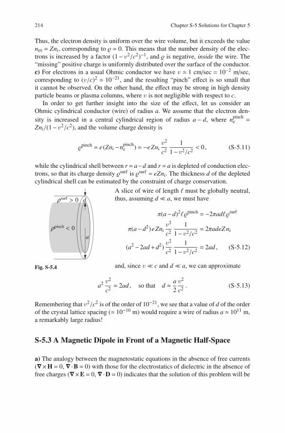
214 Chapter S-5 Solutions for Chapter 5
Thus, the electron density is uniform over the wire volume, but it exceeds the value
ne0 = Zni, corresponding to = 0. This means that the number density of the elec-
trons is increased by a factor (1− v2/c2)−1, and is negative, inside the wire. The
“missing” positive charge is uniformly distributed over the surface of the conductor.
c) For electrons in a usual Ohmic conductor we have v ≃ 1 cm/sec = 10−2 m/sec,
corresponding to (v/c)2 ≃ 10−21, and the resulting “pinch” effect is so small that
it cannot be observed. On the other hand, the effect may be strong in high density
particle beams or plasma columns, where v is not negligible with respect to c.
In order to get further insight into the size of the effect, let us consider an
Ohmic cylindrical conductor (wire) of radius a. We assume that the electron den-
sity is increased in a central cylindrical region of radius a − d, where npinche =
Zni/(1−v2/c2), and the volume charge density is
pinch = e (Zni−npinche ) = −eZni
v2
c2
1
1−v2/c2
< 0 , (S-5.11)
while the cylindrical shell between r = a−d and r = a is depleted of conduction elec-
trons, so that its charge density surf is surf = eZni. The thickness d of the depleted
cylindrical shell can be estimated by the constraint of charge conservation.
a
dρsurf > 0
ρpinch < 0
Fig. S-5.4
A slice of wire of length ℓ must be globally neutral,
thus, assuming d≪ a, we must have
π(a−d)2ℓpinch = −2πadℓsurf
π(a−d2)eZniv
2
c2
1
1−v2/c2
= 2πadeZ ni
(a2−2ad+d2)v
2
c2
1
1−v2/c2
= 2ad , (S-5.12)
and, since v≪ c and d≪ a, we can approximate
a2 v2
c2≃ 2ad , so that d ≃
a
2
v2
c2. (S-5.13)
Remembering that v2/c2 is of the order of 10−21, we see that a value of d of the order
of the crystal lattice spacing (≃ 10−10 m) would require a wire of radius a ≃ 1011 m,
a remarkably large radius!
S-5.3 A Magnetic Dipole in Front of a Magnetic Half-Space
a) The analogy between the magnetostatic equations in the absence of free currents
(∇×H = 0, ∇ ·B = 0) with those for the electrostatics of dielectric in the absence of
free charges (∇×E = 0, ∇ ·D = 0) indicates that the solution of this problem will be

S-5.3 A Magnetic Dipole in Front of a Magnetic Half-Space 215
−dO
y
m
−d
y
m
x+d
x
m
x < 0 x > 0
µr
O
Fig. S-5.5
similar to that of Prob-
lem (3.2). Thus, analo-
gously to Problem (3.2),
we treat the vacuum half-
space and the medium-
filled half-space separately,
with separate educated
guesses for the magnetic
field in each half-space.
This in order to exploit the uniqueness theorem for the Poisson equation (5.5). Our
guess for half-space 1 (x < 0) is that the field is same as if the magnetic medium
were removed from half-space 2 (thus, vacuum in the whole space), and replaced
by an image magnetic dipole m′ located symmetrically to m with respect to the
x = 0 plane, at x = d. Our guess for half-space 2 (x > 0) is that the field is the same
as if the magnetic medium filled the whole space, and the magnetic dipole m were
replaced by a different magnetic dipole m′′, placed at the same location. Thus we
look for values of m′ and m′′ originating a magnetic field B1 in half-space 1, and a
magnetic field B2 in half-space 2, satisfying the interface conditions at x = 0
B1⊥(x = 0−) = B2⊥(x = 0+) , B1‖(x = 0−) =1
μrB2‖(x = 0+) , (S-5.14)
The subscripts ‖ and⊥ stand for parallel and perpendicular to the x= 0 plane, respec-
tively. Thus, at a generic point P ≡ (0,y,z) of the x = 0 plane, we must have
Bx(0−,y,z) = Bx(0+,y,z)
By(0−,y,z) =1
μrBy(0+,y,z)
Bz(0−,y,z) =
1
μrBz(0
+,y,z) . (S-5.15)
The field generated by a magnetic dipole m in a medium of relative magnetic per-
mittivity μr is
B(r) =km
bmμr
3(m · r) r−m
r3(S-5.16)
where r is the distance vector directed from m to the point where we evaluate the
field, and r = r/r is the unit vector along r. Note that, differently from Problem
O
y
O
y
x x
x < 0 x > 0
µr
d
m
r
B
Bmθ
d
m
d
r Bθr
Fig. S-5.6
(3.2), here we do not have
cylindrical symmetry around
the x axis, because the real
magnetic dipole m is not lying
on x. It is convenient to intro-
duce the angles θ = arcsin(d/r)
and φ = arctan(z/y), and write
the Cartesian components of B
separately

216 Chapter S-5 Solutions for Chapter 5
Bx =km
bmμr
3mcosθ sinθ
r3
By =km
bmμr
3mcos2 θcosφ−m
r3
Bz =km
bmμr
3mcos2 θ sinφ
r3, (S-5.17)
where r =√
d2+ y2+ z2. If we replace (S-5.17) into (S-5.15) and divide by (km/bm)
the boundary conditions become
3mcosθ sinθ
r3−
3m′ cosθ sinθ
r3= μr
3m′′ cosθ sinθ
r3
3mcos2 θcosφ−m
r3+
3m′ cos2 θcosφ−m′
r3=
3m′′ cos2 θcosφ−m′′
r3
3mcos2 θ sinφ
r3+
3m′ cos2 θ sinφ
r3=
3m′′ cos2 θ sinφ
r3, (S-5.18)
which can be further simplified into
m−m′ = μr m′′
m+m′ =m′′ (S-5.19)
leading to the solution
m′ = −μr−1
μr+1m , m′′ =
2
μr+1m . (S-5.20)
As expected, the expressions for m′ and m′′ as functions of m are identical to (S-3.8)
for the image charges q′ and q′′ as functions of the real charge q (although Prob-
lem 3.2 involves point charges, the generalization to electric dipoles is immediate).
b) The force exerted by the magnetic half-space on m equals the force that would
be exerted on m by a real magnetic dipole m′ located at x = +d. The force between
two magnetic dipoles at a distance r from each other is
f = −km
bm∇
[
m ·m′−3(m · r)(m′ · r)
r3
]
, (S-5.21)
with, in our case, r = x, r = 2d, and m · r =m′ · r = 0, so that the force on m is
f = −km
bm
3m2
r4
(
μr−1
μr+1
)
x =km
bm
3m2
16d4
(
μr−1
μr+1
)
x . (S-5.22)
The force is repulsive (antiparallel to x) for μr < 1 (diamagnetic material), and attrac-
tive (parallel to x) for μr > 1 (paramagnetic material). At the limit μr → 0 we have
a perfect diamagnetic material (superconductor), and m′ →m, the two dipoles are
parallel and the force is repulsive, as expected. In this case m′′ 0, so that H 0

S-5.3 A Magnetic Dipole in Front of a Magnetic Half-Space 217
in the half-space 2, where, however, μr = 0 so that B = μ0μrH = 0. The situation
is opposite to that of a perfect conductor in electrostatics, where an electric dipole
would induce an opposite image dipole, and the force would be attractive.
At the limit of μr → ∞ (perfect ferromagnetic material), we have m′ → −m,
corresponding to an attractive force, while m′′→ 0 and H→ 0 inside the material.
This situation is analogous to the case of a conductor in electrostatics. Notice that B
is finite inside the material (since μrm′′→ 2m) and given by
B =km
bmμr
3 r (r ·m′′)−m′′
4πr3→ 2
3 r (r ·m)−m
4πr3, (x > 0) , (S-5.23)
so that the paramagnetic material doubles the value of the magnetic field in vacuum
in the limit μr→∞.
S-5.4 Magnetic Levitation
a) The radial component Br of the magnetic field close to the z axis can be eval-
uated by applying Gauss’s law ∇ ·B = 0 to a small closed cylinder of radius r,
coaxial with the z axis, and with the bases at z and z+∆z, as shown in Fig. S-5.7.
The flux of B through the total surface of the cylinder must be zero, thus we have
z
z + ∆z
z
r
Bz(z + ∆ z)
Bz(z)
Br(r)
Fig. S-5.7
0 =
∮
cylinder
B ·dS (S-5.24)
= 2πr∆zBr(r)+πr2 [Bz(z+∆z)−Bz(z)]
,
leading to
Br = −r[
Bz(z+∆z)−Bz(z)]
2∆z
≃ −B0
2Lr (S-5.25)
b) According to Table 5.1, the force exerted by an external magnetic field B on
a magnetic dipole m is f = (m ·∇)B. If we assume that the dipole is moving in a
region free of electric current densities, so that ∇×B = 0, the work done on the
dipole when it performs an infinitesimal displacement dr ≡ (dx,dy,dz) is1
1We have
dW = [(m ·∇)B] ·dr =∑
i, j
mi ∂iB j dx j =∑
i, j
mi ∂ jBi dx j =∑
i
mi dBi =m ·dB, (S −5.26)
where, as usual, x1,2,3 = x,y,z, and ∂1,2,3 = ∂x,∂y,∂z. We have used the property ∂iB j = ∂ jBi, trivial
for i = j, while the condition ∇×B = 0 implies ∂iB j −∂ jBi = 0 also for i j.

218 Chapter S-5 Solutions for Chapter 5
dW = f ·dr = [(m ·∇)B] ·dr =m ·dB. (S-5.27)
For a permanent magnetic dipole this leads to the well known expression for the
potential energy of a dipole located at r
U(r) = −m ·B(r). (S-5.28)
Here, however, the magnetic dipole is not permanent. Rather, we have an induced
dipole m = αB. Thus we have
U(r2)−U(r1) = −
∫ r2
r1
m ·dB = −α
∫ r2
r1
B ·dB = −α
2
∫ r2
r1
dB2 (S-5.29)
=α
2
[
B2(r1)−B2(r2)]
=1
2[m(r1) ·B(r1)−m(r2) ·B(r2)] .
and the potential energy for the induced dipole at r is written
U(r) = −1
2m(r) ·B(r) . (S-5.30)
For the present problem, this leads to
U(r) = −1
2m(r) ·B(r) = −
1
2αB2(r) = −
1
2
αB20
L2
(
z2+r2
4
)
. (S-5.31)
c) The potential energy U has a minimum in the origin (r = 0,z = 0) if α < 0 (dia-
magnetic particle). The force is
f = −∇U = −1
2|α|
2B20
L2
(
z z+r
4r
)
. (S-5.32)
Thus, we have a harmonic force both for radial and axial displacements, with corre-
sponding oscillation frequencies
ωz =
√
|α|B20
ML2, ωr =
ωz
2. (S-5.33)

S-5.5 Uniformly Magnetized Cylinder 219
S-5.5 Uniformly Magnetized Cylinder
M
R
n
Km
Fig. S-5.8
a) The volume magnetization current (bound cur-
rent) density Jm is zero all over the cylinder volume
because the cylinder magnetization M is uniform,
and Jm = ∇×M/bm. For the surface magnetization
current density Km we have Km =M× n/bm, where
n is the unit vector perpendicular to the cylinder lat-
eral surface, and bm is the system dependent constant
defined in (5.1). Since M and n are perpendicular to
each other, we have Km = |Km| = |M|/bm.
b) The magnetized cylinder is equivalent to a
solenoid with nI = Km, where n is the number of
coils per unit length, and I is the electric current cir-
culating in each coil. Thus, at the h ≫ R limit, the
magnetic field is uniformly zero outside the cylinder, and it is uniform and equal to
B =4πkm
bmnI =
4πkm
bmKm =
4πkm
bmM =
μ0M , SI
4πM , Gaussian,(S-5.34)
inside. The auxiliary field H is zero both inside and outside the cylinder because
Hin =
⎧
⎪
⎪
⎪
⎪
⎨
⎪
⎪
⎪
⎪
⎩
Bin
μ0−M = 0 , SI
Bin−4πM = 0 , Gaussian.
Hout =
⎧
⎪
⎪
⎪
⎪
⎨
⎪
⎪
⎪
⎪
⎩
Bout
μ0= 0 , SI
Bout = 0 , Gaussian.
(S-5.35)
c) At the “flat cylinder” limit, R≫ h, the cylinder is equivalent to a single coil of
radius R carrying a current I = hKm = hM/bm. Thus we have for the field at its center
B0 = 2πkmI
R=
⎧
⎪
⎪
⎪
⎪
⎪
⎪
⎨
⎪
⎪
⎪
⎪
⎪
⎪
⎩
μ0I
2R=μ0Mh
2R, SI
2πI
cR=
2πMh
cR, Gaussian,
(S-5.36)
and B0 approaches zero as h/r→ 0.
d) The equivalent magnetic charge density is defined as m = −∇ ·M, thus m ≡ 0
inside the cylinder volume, while the two bases of the cylinder carry surface mag-
netic charge densitiesσm =M · n=±M. Therefore our flat magnetized cylinder is the
“magnetostatic” equivalent of an electrostatic parallel-plate capacitor. The equiva-
lent magnetic charge “generates” the auxiliary magnetic field H, which is uniform,
and equal to H =−σm =−M, inside the volume of the flat cylinder, and zero outside.
Thus B = μ0(H+M) is zero everywhere (more realistically, it is zero far from the
boundaries).
The field of a magnetized cylinder and its electrostatic analog are further dis-
cussed in Problem 13.1.

220 Chapter S-5 Solutions for Chapter 5
S-5.6 Charged Particle in Crossed Electric and Magnetic Fields
a) We choose a Cartesian laboratory frame of reference xyz with the y axis parallel
to the electric field E, the z axis parallel to the magnetic field B, and the origin O
located so that the particle is initially at rest in O. The Lorentz force on the particle
f = q [E+bmv×B]
has no z component, and the motion of the particle occurs in the xy plane. The
equations of motion are thus
mx = bmqBy ,
my = −bmqB x+qE . (S-5.37)
It is convenient to introduce two new variables x′, and y′, such that
x = x′+v0 t , y = y′ , (S-5.38)
where v0 is a constant velocity, which we shall determine in order to simplify the
equations of motion. The initial conditions for the primed variables are
x′(0) = 0 , x′(0) = −v0 ,
y′(0) = 0 , y′(0) = −0 . (S-5.39)
Differentiating (S-5.38) with respect to time we obtain
x = v0+ x′ , x = x′ ,
y = y′ , y = y′ , (S-5.40)
which we substitute into (S-5.37), thus obtaining the following equations for the
time evolution of the primed variables
m x′ = bmqBy′ ,
my′ = −bmqBv0−bmqB x′+qE . (S-5.41)
Now we choose the constant velocity v0 to be
v0 =E
bmB=
⎧
⎪
⎪
⎪
⎪
⎪
⎨
⎪
⎪
⎪
⎪
⎪
⎩
E
B, SI,
E
Bc , Gaussian ,
(S-5.42)
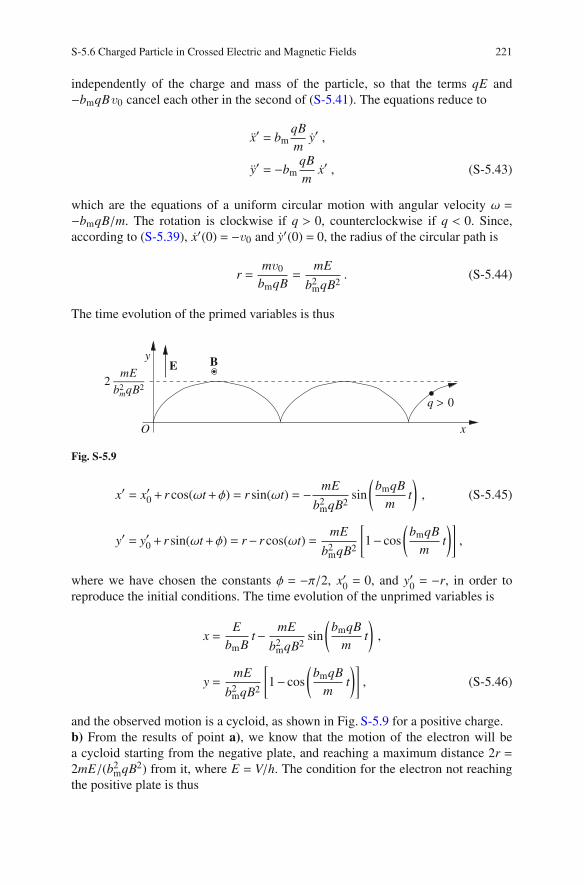
S-5.6 Charged Particle in Crossed Electric and Magnetic Fields 221
independently of the charge and mass of the particle, so that the terms qE and
−bmqBv0 cancel each other in the second of (S-5.41). The equations reduce to
x′ = bmqB
my′ ,
y′ = −bmqB
mx′ , (S-5.43)
which are the equations of a uniform circular motion with angular velocity ω =
−bmqB/m. The rotation is clockwise if q > 0, counterclockwise if q < 0. Since,
according to (S-5.39), x′(0) = −v0 and y′(0) = 0, the radius of the circular path is
r =mv0
bmqB=
mE
b2mqB2
. (S-5.44)
The time evolution of the primed variables is thus
O x
q > 0
y
2mE
b2mqB2
E B
Fig. S-5.9
x′ = x′0+ r cos(ωt+φ) = r sin(ωt) = −mE
b2mqB2
sin
(
bmqB
mt
)
, (S-5.45)
y′ = y′0+ r sin(ωt+φ) = r− r cos(ωt) =mE
b2mqB2
[
1− cos
(
bmqB
mt
)]
,
where we have chosen the constants φ = −π/2, x′0= 0, and y′
0= −r, in order to
reproduce the initial conditions. The time evolution of the unprimed variables is
x =E
bmBt−
mE
b2mqB2
sin
(
bmqB
mt
)
,
y =mE
b2mqB2
[
1− cos
(
bmqB
mt
)]
, (S-5.46)
and the observed motion is a cycloid, as shown in Fig. S-5.9 for a positive charge.
b) From the results of point a), we know that the motion of the electron will be
a cycloid starting from the negative plate, and reaching a maximum distance 2r =
2mE/(b2mqB2) from it, where E = V/h. The condition for the electron not reaching
the positive plate is thus
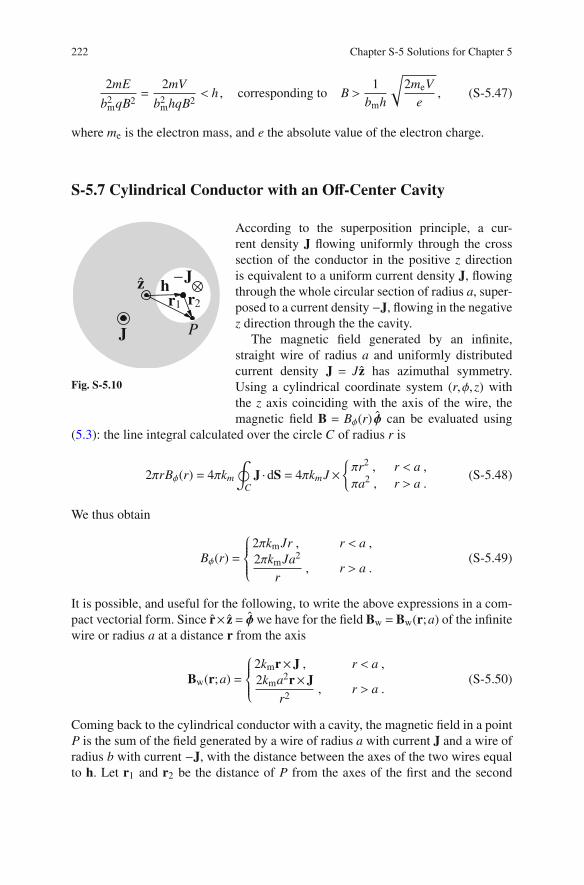
222 Chapter S-5 Solutions for Chapter 5
2mE
b2mqB2
=2mV
b2mhqB2
< h , corresponding to B >1
bmh
√
2meV
e, (S-5.47)
where me is the electron mass, and e the absolute value of the electron charge.
S-5.7 Cylindrical Conductor with an Off-Center Cavity
r2
hr1
PJ
−Jz
Fig. S-5.10
According to the superposition principle, a cur-
rent density J flowing uniformly through the cross
section of the conductor in the positive z direction
is equivalent to a uniform current density J, flowing
through the whole circular section of radius a, super-
posed to a current density −J, flowing in the negative
z direction through the the cavity.
The magnetic field generated by an infinite,
straight wire of radius a and uniformly distributed
current density J = Jz has azimuthal symmetry.
Using a cylindrical coordinate system (r,φ,z) with
the z axis coinciding with the axis of the wire, the
magnetic field B = Bφ(r) φ can be evaluated using
(5.3): the line integral calculated over the circle C of radius r is
2πrBφ(r) = 4πkm
∮
C
J ·dS = 4πkmJ×
πr2 , r < a ,
πa2 , r > a .(S-5.48)
We thus obtain
Bφ(r) =
⎧
⎪
⎪
⎪
⎨
⎪
⎪
⎪
⎩
2πkmJr , r < a ,
2πkmJa2
r, r > a .
(S-5.49)
It is possible, and useful for the following, to write the above expressions in a com-
pact vectorial form. Since r× z= φwe have for the field Bw =Bw(r;a) of the infinite
wire or radius a at a distance r from the axis
Bw(r;a) =
⎧
⎪
⎪
⎪
⎨
⎪
⎪
⎪
⎩
2kmr×J , r < a ,
2kma2r×J
r2, r > a .
(S-5.50)
Coming back to the cylindrical conductor with a cavity, the magnetic field in a point
P is the sum of the field generated by a wire of radius a with current J and a wire of
radius b with current −J, with the distance between the axes of the two wires equal
to h. Let r1 and r2 be the distance of P from the axes of the first and the second

S-5.7 Cylindrical Conductor with an Off-Center Cavity 223
wire, respectively, we have r1 − r2 = h. We thus have B(P) = Bw(r1;a)+Bw(r2;b).
In particular, inside the cavity we have r1 < a and r2 < b, thus
B(P) = 2kmr1 ×J+2kmr2 × (−J) = 2km(r1 − r2)×J = 2kmh×J , (S-5.51)
which is a constant vector. Thus, inside the cavity the magnetic field is uniform and
perpendicular to both J and h.
S-5.8 Conducting Cylinder in a Magnetic Field
a) We use a cylindrical coordinate system (r,φ,z), with the z axis along the cylinder
axis. The centrifugal force, Fc, and the magnetic force, Fm, are both directed along
r and depend on r only:
Fc = meω2r , Fm = −ev×B0 = −eωB0r ,
|Fc|
|Fm|=
meω
eB0≃ 7.2×10⁻⁵ . (S-5.52)
The magnetic force is dominant, and we shall neglect the centrifugal force in the
following.
b) In static conditions the magnetic force must be compensated by an electric field
E
E = −v×B0 = −ωB0r . (S-5.53)
The existence of this electric field implies a uniform charge density
=1
4πke∇ ·E =
E(r)
2πker= −ωB0
2πke. (S-5.54)
Since the cylinder carries no net charge, its lateral surface must have a charge density
σ = −πa2h
2πah= −
a
2=ωaB0
4πke. (S-5.55)
a
r
ω
J(r)
dr
K
Fig. S-5.11
c) The volume charge density is associated to a vol-
ume rotational current density J(r) due to the cylin-
der rotation
J(r) = ωrφ = −ω2rB0
2πkeφ . (S-5.56)
The contribution of J(r) to the magnetic field on the
cylinder axis, BJ , can be evaluated by dividing the

224 Chapter S-5 Solutions for Chapter 5
cylinder into infinitesimal coaxial cylindrical shells between r and r+dr. Each shell
is equivalent to a solenoid of radius r and product nI = J(r)dr, contributing dBJ =
4πkmJ(r)dr to the field at its inside. The total contribution of J(r) at a distance r
from the axis is thus
BJ(r) = 4πkm
∫ a
r
J(r′)dr′ = −4πkmω2B0
2πke
∫ a
r
r′ dr′
= −4πkmω2B0
2πke
[
r′2
2
]a
r
= −km
keω2B0(a2− r2) . (S-5.57)
Now we must add the contribution BK of the surface current density K = σωa
BK = 4πkmσωa = 4πkmωaωaB0
4πke=
km
keω2a2B0 (S-5.58)
and the total magnetic field B1(r) due to the rotational currents is
B1(r) = BJ(r)+BK =km
keω2B0 r2 , (S-5.59)
which is zero on the axis and reaches its maximum value at r = a−. We thus have
B1(a−)
B0=
km
keω2a2 =
ω2a2
c2≃ (2.1×10⁻⁷)2≪ 1 . (S-5.60)
S-5.9 Rotating Cylindrical Capacitor
ab
ω
h
z
Q
−Q
K
−K
Fig. S-5.12
a) We use cylindrical coordinates (r,φ,z) with the z
axis coinciding with capacitor axis. We assume ω =
ω z, with ω = 2π/T > 0. The surface currents due to
the capacitor rotation are thus
K = σv =Q
2πahωa =
Q
hT, (S-5.61)
where σ = Q/(2πah) is the surface charge density
on the inner shell, and −K on the outer shell, inde-
pendently of a and b. Thus the two cylindrical shells
are equivalent to two solenoids with nI products
nI = ±K, respectively. The outer shell gives origin to
a magnetic field Bb = −4πkmK z in the region r < b,
and to no field in the region r > b. The inner shell

S-5.9 Rotating Cylindrical Capacitor 225
gives origin to a field Ba = −Bb in the region r < a, and to no field in the region
r > b. The total field B = Ba+Bb is thus
B =
⎧
⎪
⎪
⎨
⎪
⎪
⎩
−4πkmK z = −4πkmQ
hTz , a < r < b ,
0 , r < a , r > b.(S-5.62)
b) The electric field is zero for r < a and r > b, while it is E(r) = r2keQ/(hr) for
a < r < b, and the force between the two shells is attractive. The electrostatic force
per unit area on, for instance, the external shell is thus
f(e)s = σb
E(b)
2= −r
Q
2πbh
2keQ
hb= −r
keQ2
πb2h2, (S-5.63)
where σb is the surface charge density on the shell. The magnetic force per unit area
on the same shell is
f(m)s = σb v×B = r
Q
2πbh
2πb
T4πkm
Q
hT= 4πkm
Q2
h2T 2, (S-5.64)
directed opposite to the electrostatic force. The ratio f(m)s / f
(e)s on the outer shell is
f(m)s
f(e)s
= 4πkmQ2
h2T 2
πb2h2
keQ2=
km
ke
(
2πb
T
)2
=v
2b
c2(S-5.65)
where vb = 2πb/T is the tangential velocity of the outer shell. The ratio (S-5.65) is
thus negligibly small in all practical cases.
S-5.10 Magnetized Spheres
a) The quickest way to obtain the solution is to exploit the analogy of the magneto-
static equations ∇×H = 0, ∇ ·B = 0 with the electrostatic ones ∇×E = 0, ∇ ·D = 0
(see also Problem 5.3), along with the definitions (3.4) and (5.19). The spatial distri-
bution of M is the same as that of P in Problem (3.3), and the boundary conditions
for H are the same as for E. Thus from (S-3.13) we immediately obtain that inside
the sphere (r < R) the field H is uniform with constant value H(int), given by
H(int) =
⎧
⎪
⎪
⎪
⎪
⎪
⎨
⎪
⎪
⎪
⎪
⎪
⎩
−M
3, SI ,
−4πM
3, Gaussian .
(S-5.66)

226 Chapter S-5 Solutions for Chapter 5
Using (5.19) we obtain for the magnetic field inside the sphere
B(int) =
⎧
⎪
⎪
⎪
⎪
⎪
⎨
⎪
⎪
⎪
⎪
⎪
⎩
2μ0M
3, SI ,
8πM
3, Gaussian .
(S-5.67)
Outside the sphere the field is that of a magnetic dipole m =M(4πR3/3) located at
the center of the sphere (r = 0).
b) The rotation of the sphere with uniform surface charge σ = Q/(4πR2) generates
an azimuthal surface current
Krot = σv = σRωsinθ φ , (S-5.68)
where θ = 0 corresponds to the direction of M. This surface current distribution
current is analogous to that of the magnetization current distribution (5.17) for the
magnetized sphere of point a),
Km =M× r = M sinθ φ . (S-5.69)
Thus, the magnetic field generated by Krot is the same as that generated by Km, with
the replacement M = σRω = Qω/(4πR).
c) Analogously to Problem 3.4 for a dielectric sphere in an external electric field, we
assume that the induced magnetization M = χmH is uniform and parallel to B0. The
total field will be the sum of the external field B0 ≡ [μ0]H0 (with [μ0] replaced by
unity for Gaussian units) and of that generated by the magnetization. Thus, inside
the sphere H is uniform and has the value H(int) given by
H(int) =
⎧
⎪
⎪
⎪
⎪
⎪
⎨
⎪
⎪
⎪
⎪
⎪
⎩
H0−M
3=H0−
χm
3H(int) , SI ,
H0−4πM
3=H0−
4πχm
3H(int) , Gaussian .
(S-5.70)
Solving for H(int) and finally using B(int) = [μ0]μrH(int) we obtain
H(int) =3
μr+2H0 , B(int) =
3μr
μr +2B0 , (S-5.71)
independently of the system of units; it may be interesting to compare the result
with (S-3.21) for the dielectric sphere. The magnetization is given by M = χmH(int).
In the case of a perfectly diamagnetic sphere (a superconducting sphere) we have
μr = 0 and B(int) = 0, and the magnetization is
M =3χm
2H0 = −
3
8π
bm
kmB0 . (S-5.72)

S-5.10 Magnetized Spheres 227
Actually, inside the sphere the external field is completely screened by the surface
currents (S-5.69) due to the magnetization (S-5.72).
It is instructive to double check the above solution by verifying the boundary
conditions at the surface of the sphere, analogously to the dielecric case of Solution
S-3.4. We choose a spherical coordinate system (r, θ,φ) with the zenith direction z
parallel to the external magnetic field B0, and the origin at the center of the sphere O,
B0
µr
O R
z φ
rrθ
θ
Fig. S-5.13
as shown in Fig. S-5.13. As an educated guess, we
look for a solution where i) the magnetic field inside
the sphere, B(int), is uniform and proportional to
B0, and, accordingly, ii) the magnetization M of the
sphere, proportional to B(int), is uniform, and iii) the
total external field, B(ext), is the superposition of the
applied external field B0 and of the field B(mag), gen-
erated by the sphere magnetization. Thus, B(mag) will
be the field generated by a magnetic dipole m = αB0
located at the center of the sphere, with α a constant
to be determined. Summing up, we are looking for a
solution
B(int) = ψB0 ,
B(ext) = B0+B(mag) , (S-5.73)
with ψ a further constant to be determined. B(mag) and its spherical components are
B(mag) = αB0km
bm
[(
3z · r
r5
)
r−z
r3
]
, (S-5.74)
B(mag)r = αB0
km
bm
2cosθ
r3, (S-5.75)
B(mag)
θ= αB0
km
bm
sinθ
r3, (S-5.76)
B(mag)
φ= 0 , (S-5.77)
where km/bm = μ0/(4π) in SI units, and km/bm = 1 in Gaussian units. The constants
α and ψ are determined from the boundary conditions on B and B/μr at the surface
of the sphere
B(int)⊥ (R, θ) = B
(ext)⊥ (R, θ) ,
B(int)
‖(R, θ)
μr= B
(ext)
‖(R, θ) , (S-5.78)

228 Chapter S-5 Solutions for Chapter 5
which lead to
ψB0 cosθ = B0 cosθ+B(mag)r (R, θ) = B0 cosθ
(
1+αkm
bm
2
R3
)
, (S-5.79)
ψB0
μrsinθ = B0 sinθ−B
(mag)
θ(R, θ) = B0 sinθ
(
1−αkm
bm
1
R3
)
. (S-5.80)
Dividing (S-5.79) by B0 cosθ, and (S-5.80) by B0 sinθ, we obtain
ψ = 1+αkm
bm
2
R3,
ψ
μr= 1−α
km
bm
1
R3, (S-5.81)
with solutions
ψ =3μr
μr +2, α = R3 bm
km
(
μr−1
μr+2
)
=
⎧
⎪
⎪
⎪
⎪
⎪
⎪
⎨
⎪
⎪
⎪
⎪
⎪
⎪
⎩
4πR3
μ0
(
μr−1
μr+2
)
, SI,
R3
(
μr−1
μr+2
)
, Gaussian,
(S-5.82)
which eventually lead to
B(int) =3μr
μr+2B0 , m =
4πR3
3M = R3 bm
km
(
μr −1
μr +2
)
B0 . (S-5.83)

Chapter S-6
Solutions for Chapter 6
S-6.1 A Square Wave Generator
a) The motion is periodic, and we choose the origin of time, t = 0, at an instant
when the coil surface is completely in the x 0 half of the xy plane. With this
choice, the flux of the magnetic field through the coil, Φ(t), increases with time
when 2nπ<ωt< (2n+1)π, with n any integer, and equalsΦ(t)= B(ωt mod 2π)a2/2.
Here, (x mod y) stands for the remainder of the division of x by y with an integer
quotient. When (2n+1)π < ωt < (2n+2)π, the flux decreases with time and equals
Φ(t) = B[2π− (ωt mod 2π)
]a2/2. The electromotive force in the coil, E(t), is thus
I
− I0
I0
2T
tT
0
Fig. S-6.1
y
x
I
I
f
B
O
y
xI
I
f O
B
Fig. S-6.2
E(t) = −bmdΦ(t)
dt(S-6.1)
= −bmBa2ω
2sign[π− (ωt mod 2π)] ,
where sign(x) = x/|x| is the sign function.
Thus, E reverses its sign whenever ωt =
nπ, with n any integer. The current cir-
culating in the coil is I = E/R. As shown
in Fig. S-6.1, I (as well as E) is a square
wave of period T = 2π/ω, and amplitude
I0 =E0
R= bm
Bωa2
2R. (S-6.2)
b) The external torque applied to the coil
in order to keep its angular velocity con-
stant must balance the torque exerted by
the magnetic forces. The magnetic force
on a current-carrying circuit element dℓ is
df = bmI dℓ×B, and is different from zero
c© Springer International Publishing AG 2017
A. Macchi et al., Problems in Classical Electromagnetism,
DOI 10.1007/978-3-319-63133-2 19
229

230 S-6 Solutions for Chapter 6
only in the x < 0 half plane. The corresponding torque dτ = r×df = b2mIr× (dℓ×B),
where r is the distance of the coil element dℓ from the z axis, is always equal to zero
on the circumference arc of the coil because the three vectors of the triple product
are mutually perpendicular here. Thus, dτ is different from zero only on the half of
the straight part of the coil inside the magnetic field, where dℓ = dr. Here we have
dτ = −b2mI0rBdr z, as shown in Fig. S-6.2, and the total torque on the coil, τ, is
τ =
∫dτ = −b2
mωB2a2
2Rz
∫ a
0
r dr = −b2mω
B2a4
4Rz , (S-6.3)
corresponding to a power dissipation
Pdiss = −τ ·ω = b2mω
2 B2a4
4R= RI2
0 , (S-6.4)
that equals the power dissipated by Joule heating. The power dissipation is con-
stant in time, neglecting the “abrupt” transient phases at t = nπ/ω, where I instantly
changes sign. Thus, the external torque must provide the power dissipated by Joule
heating.
c) If we take the coil self-inductance L into account, the equation for the current in
the coil becomes
E(t)−LdI
dt= RI , (S-6.5)
where E(t) is the electromotive force (S-6.1), due to the flux change of the external
field only. However “small” L may be, its contribution is not negligible because, if
I were an ideal square wave, its derivative dI/dt would diverge whenever t = nπ/ω
(instantaneous transition between −I0 and +I0). The general solution of (S-6.5) is,
taking into account that E(t) is constant over each half-period,
I =ER+Ke−t/t0 , (S-6.6)
T 2T
t
I
I0
0
−I0
Fig. S-6.3
where t0 = L/R is the characteristic
time of the loop, and K is a constant
to be determined from the initial con-
ditions. If L is small enough, we can
assume that at time t = 0− we have
E(t) = +E0 and I(t) = +I0. At time
t = 0, E(t) switches instantaneously
from +E0 to −E0, and the constant K
is determined by the initial condition
I(0) = I(0−) = I0 = E0/R, leading to
K = 2E0/R. Thus, for 0 < t < π/ω,

S-6.1 A Square Wave Generator 231
I(t) = I0 (2e−t/t0 −1) . (S-6.7)
T 2T
0
I
t
I0
IM
−I0
−IM
Fig. S-6.4
At t = (π/ω)− we have E(t) = −E0
and we can assume that I(t) = −I0. At
t = π/ω E(t) switches instantaneously
from −E0 to +E0, and, for π/ω < t <
2π/ω, we have
I(t) = −I0 (2e−(t−π/ω)/t0 −1) , (S-6.8)
and so on for the successive periods.
The self-inductance of the coil prevents the current from switching instantaneously
between +I0 and −I0: the change occurs following an exponential with characteristic
time t0 = L/R.
The behavior described by (S-6.7) and (S-6.8) is valid only if t0≪ T = 2π/ω, as
in Fig. S-6.3, representing the case of t0 = 0.04T . If t0 is not negligible with respect
to T , the current oscillates between two values +IM and −IM , with IM < I0. Let us
consider the time interval 0 ≤ t ≤ π/ω. We must have I(0) = IM and I(π/ω) = −IM .
Replacing I by (S-6.6), we obtain
IM = I01− e−T/2t0
1+ e−T/2t0. (S-6.9)
The plot of I(t) can no longer be approximated by a square wave, as shown in
Fig. S-6.4 for the case t0 = 0.25T .
S-6.2 A Coil Moving in an Inhomogeneous Magnetic Field
a) With our assumptions, the flux of the magnetic field through the coil can be
approximated as
ΦB(t) =ΦB[z(t)] ≃ πa2B0z(t)
L= πa2B0
z0+ vt
L, (S-6.10)
where z0 is the position of the center of the coil at t = 0. The rate of change of this
magnetic flux is associated to an electromotive force E, and to a current I = E/Rcirculating in the coil
E = RI = −bmdΦ
dt= −bm πa
2B0v
L. (S-6.11)
b) The power dissipated by Joule heating is
P = RI2 =E2
R= b2
m
(πa2B0 v)2
L2R. (S-6.12)

232 S-6 Solutions for Chapter 6
Thus, in order to keep the coil in motion at constant speed, one must exert an external
force fext on the coil, whose work compensates the dissipated power. We have
fext · v = P = b2m
(πa2B0 v)2
L2R, (S-6.13)
and the coil is submitted to a frictional force proportional to its velocity
ffrict = −fext = −b2m
(πa2B0)2
L2Rv . (S-6.14)
c) The force ffrict is actually the net force obtained by integrating the force dffrict =
bm I dℓ ×B acting on each coil element dℓ:
ffrict = bm I
∮
coil
dℓ×B . (S-6.15)
ad
I
z
B(r, z)
Fig. S-6.5
The contribution of the z component of B is
a radial force tending to shrink the coil if
∂tΦ > 0, or to widen it if ∂tΦ < 0, accord-
ing to Lenz’s law; the case represented in
Fig. S-6.5 corresponds to the latter case. Thus
fext, directed along z, is due only to the radial
component Br of B. The component Br is
not given by the problem, but, as we saw at
answer a) of Problem 5.4, it can be evaluated
by applying Gauss’s law to a closed cylindri-
cal surface of radius r and height ∆z. According to (S-5.25)
Br ≃ −B0
2Lr , thus dffrict = bm I dℓ
B0 a
2L, (S-6.16)
and by substituting (S-6.11) and integrating over the coil we obtain
ffrict = zbmI
∮
coil
dℓB0 a
2L= −zbm
(bmπa
2B0v
L
)(2πa
B0 a
2L
)
= −zb2m
(πa2B0)2
L2Rv , (S-6.17)
in agreement with (S-6.14).
S-6.3 A Circuit with “Free-Falling” Parts
a) We choose the x axis oriented downwards, with the origin at the location of the
upper horizontal bar, as in Fig. S-6.6. The current I in the rectangular circuit is

S-6.3 A Circuit with “Free-Falling” Parts 233
I =ER= −bm
1
R
dΦ(B)
dt= −bm
Ba
R
dx
dt= −bm
Bav
R, (S-6.18)
where x is the position of the falling bar, and v = x its velocity. The velocity is
positive, and the current I is negative, i.e., it circulates clockwise, in agreement with
Lenz’s law. The magnetic force on the falling bar is fB = bmBaI x, antiparallel to the
gravitational force mg, and the equation of motion is
mdv
dt= mg+bmBaI = mg−b2
m
(Ba)2
Rv. (S-6.19)
R/ 2
g
ax
O
R/ 2
IB
x
Fig. S-6.6
The solution of (S-6.19), with the initial condition
v(0) = 0, is
v(t) = vt
(1− e−t/τ
)(S-6.20)
where
τ =mR
(bmBa)2and vt = gτ =
mRg
(bmBa)2. (S-6.21)
As t → ∞, the falling bar approaches the terminal
velocity vt.
b) When v = vt, the power dissipated in the circuit by
Joule heating is
PJ = RI2t =
(bmBavt)2
R=
(mg
bmBa
)2
R , (S-6.22)
where It = −bmBavt/R is the “terminal current”. On
the other hand, the work done by the force of gravity per unit time is
PG = mg · vt = mgmgR
(bmBa)2= PJ , (S-6.23)
in agreement with energy conservation for the bar moving at constant velocity.
c) When both horizontal bars are falling, we denote by x1 the position of the upper
bar, and by x2 the position of the lower bar, as in Fig. S-6.7, with v1 = x1 and v2 = x2.
The current I circulating in the circuit is
I =ER= −bm
1
R
dΦ(B)
dt= −bm
Ba
R
d
dt(x2− x1)
= −bmBa
R(v2− v1), (S-6.24)

234 S-6 Solutions for Chapter 6
R/ 2
1
2
a
g
O
x
x1
x2
R/ 2
B
I
Fig. S-6.7
circulating counterclockwise (I > 0) if v1 > v2, and
clockwise (I < 0) if v1 < v2. The magnetic forces
acting on the two falling bars are fB1 = −bmBaI x
and fB2 = bmBaI x, respectively. Independently of the
sign of I, we have fB1 =−fB2, so that the net magnetic
force on the system comprising the two falling bars
is zero. The equations of motion are thus
mdv1
dt= mg+b2
m
(Ba)2
R(v2− v1) (S-6.25)
mdv2
dt= mg−b2
m
(Ba)2
R(v2− v1) , (S-6.26)
with the initial conditions v1(0) = v0 and v2(0) = 0.
The sum of equations (S-6.25) and (S-6.26) is
d
dt(v1+v2)= 2g , with solution
v1+ v2
2=
v0
2+gt ,
(S-6.27)
meaning that the center of mass of the two horizontal bars follows a free fall, inde-
pendent of the magnetic field B. On the other hand, the difference of equations
(S-6.25) and (S-6.26) is
d
dt(v1− v2) = −2
τ(v1− v2) , with solution v1− v2 = v0 e−2t/τ , (S-6.28)
where τ = mR/(bmBa)2. For the velocities of the two horizontal bars we obtain
v1 =v0
2
(1+ e−2t/τ
)+gt , v2 =
v0
2
(1− e−2t/τ
)+gt . (S-6.29)
At the steady state limit (t≫ τ) we have
limt→∞
v1 = limt→∞
v2 =v0
2+gt and lim
t→∞I = 0 , (S-6.30)
since, for v1 = v2, the flux of B through the loop is constant.
S-6.4 The Tethered Satellite
a) To within our approximations, we can assume that the magnetic field is constant
over the satellite orbit, and equal to the field at the Earth’s equator, Beq ≃ 3.2×10⁻⁵ T. The field is parallel to the axis of the satellite orbit, and constant over the
tether length. The electromotive force E on the tether equals the line integral of the
magnetic force along the wire,

S-6.4 The Tethered Satellite 235
E = bm
∫
tether
dℓ · v(r)×Beq = bm
∫ R⊕+h−ℓ
R⊕+h
drωr Beq , (S-6.31)
where ω = v/r is the angular velocity of the satellite. To within our approximations
we can also assume that also v(r) ≃ v(R⊕) ≃ 8000m/s is constant over the wire
length, and obtain
E ≃ bmvℓBeq =
⎧⎪⎪⎪⎨⎪⎪⎪⎩8000×1000×3.2×10−5 ≃ 250V , SI,1
c×8×105×105×0.32 ≃ 0.85statV , Gaussian.
(S-6.32)
b) Neglecting the resistance of the ionosphere, the current I circulating in the wire,
and the corresponding power dissipated by Joule heating Pdiss are, respectively,
I =ER= bm
vℓBeq
R, and Pdiss = RI2 = b2
m
v2ℓ2B2eq
R. (S-6.33)
The power dissipated in the tether by Joule heating must equal minus the work done
by the magnetic force on the wire. This can be easily verified, since the magnetic
force acting on the wire is
F = bmIℓ r×Beq = −b2m
B2eqℓ
2
Rv , (S-6.34)
and the corresponding work rate is
P = F · v = −b2m
B2eqℓ
2
Rv2 = −Pdiss . (S-6.35)
If we assume that the tether is a copper wire (conductivity σ ≃ 107 Ω−1m−1 SI,σ ≃ 9×10¹⁶ s−1 Gaussian) of cross section A=1 cm2, the magnitude of the magneticdrag force on the system is
Fdrag = b2m
B2eqℓ
2
ℓ/(σA)v =
⎧⎪⎪⎪⎪⎪⎪⎨⎪⎪⎪⎪⎪⎪⎩
(3.2×10⁻⁵)2 ×1000
1/(107 ×10−4)×8000 ≃ 8.2N , SI
1
c2
(0.32)2 ×10⁵
1/(9×1016)×8×105 ≃ 8.2×10⁵ dyn , Gaussian.
(S-6.36)
This problem gives an elementary description of the principle of the “Tethered
Satellite System”, investigated in some Space Shuttle missions as a possible gener-
ator of electric power for orbiting systems.

236 S-6 Solutions for Chapter 6
S-6.5 Eddy Currents in a Solenoid
a) The time-dependent current in the solenoid generates a time-dependent magnetic
field which, in turn, induces a time-dependent contribution to the electric field. The
induced electric field is associated to a displacement current density, and, in a con-
ductor, also to a conduction current density J = σE. Both current densities, in turn,
affect the magnetic field. According to our symmetry assumptions, in a cylindrical
coordinate system (r,φ,z), with the solenoid axis as z axis, the only non-zero com-
ponent of the magnetic field is Bz, and the only non-zero component of the electric
field is Eφ, therefore the only non-zero component of the conduction current density
is Jφ. Both Bz and Eφ depend only on r. In principle we must solve (6.1) and (6.5)
which in cylindrical coordinates yield (see Table A.1 of the Appendix),
1
r∂r(rEφ) = −bm ∂tBz , (S-6.37)
−∂rBz = 4πkmσEφ+km
ke∂tEφ . (S-6.38)
Finding the complete solution to (S-6.37) and (S-6.38) is possible but somewhat
involved. However, if the angular frequency ω of the driving current is low enough,
the slowly varying current approximation (SVCA) provides a sufficiently accurate
solution of the problem.
In the SVCA, we start by calculating B as in the static case. Neglecting boundary
effects, a DC current I would generate a uniform magnetic field B = z4πkm μrnI
inside our solenoid, and B ≡ 0 outside. Thus, inside the solenoid, we would have
B = zμ0 μrnI in SI units, and B = z4πμrnI/c in Gaussian units. If we replace I by
I0 cosωt we obtain
B(0) = z4πkm μrnI0 cosωt , (S-6.39)
which we assume as our zeroth-order approximation for the field inside the solenoid.
In the next step of SVCA, we evaluate the first order correction by calculating the
electric field E(1) induced by (S-6.39), and its associated current densities. These
current densities, in turn, contribute to the first order correction to the magnetic
field. A posteriori, our procedure will be justified if the first order correction to
the magnetic field, B(1), is much smaller than B(0). And so on for the successive
correction orders. For additional simplicity, we neglect the displacement current,
i.e., the last term on the right-hand side of (S-6.38), although its inclusion would not
be difficult.
Using (6.1) and the symmetry assumptions, the first-order electric field E(1)(r) =
φE(1)(r) can be found from its path integral over the circumference of radius r,
∮E(1) ·dℓ = 2πrE(1)(r) = −bmπr
2∂tB(0) , (S-6.40)

S-6.5 Eddy Currents in a Solenoid 237
R
rB(0)
E(1)
r
I0 cos t
Fig. S-6.8
which yields
E(1)(r) = kmbm 2πμrrnI0ωsinωt φ
=
⎧⎪⎪⎪⎪⎨⎪⎪⎪⎪⎩
μ0μr
2rnI0ωsinωtφ , SI,
1
c22πμrrnI0ωsinωt φ , Gaussian.
(S-6.41)
Notice that the induced electric field also generates
an electromotive force E(1) in the solenoid coils. We
assume the generator producing the current I(t) =
I0 cosωt to be an ideal one, which maintains the
same current against any effect occurring in the cir-
cuit (the appearance of E(1) will require extra work
to maintain the current).
b) Due to the conductivity σ of the solenoid core, the
electric field E(1)(r) originates an azimuthal current density J(1)(r) = σE(1)(r) (eddy
currents) in the material. The corresponding Joule dissipation heats up the material.
The energy turned into heat per unit volume at each instant t is
J(1)(r) ·E(1)(r) = σ[E(1)(r)
]2= σ (kmbm 2πμrrnI0ωsinωt)2 , (S-6.42)
with a time average
⟨J(1)(r) ·E(1)(r)
⟩= 2σ(kmbm πμrrnI0ω)2 . (S-6.43)
The total dissipated power is found by integrating (S-6.43) over the volume of the
cylindrical core
Pd =
∫
cylinder
⟨J(1)(r) ·E(1)(r)
⟩d3x = 2σ (kmbm πμrnI0ω)2
∫ R
0
r2ℓ2πrdr
= σπℓ(kmbm πμrnI0ωR2
)2=
⎧⎪⎪⎪⎪⎪⎨⎪⎪⎪⎪⎪⎩
σμ20μ2
r
16πn2I2
0ω2ℓR4 , SI,
1
c4π3σμ2
r n2I20ω
2ℓR4 , Gaussian.
(S-6.44)
c) The induced current density J(1)(r) = σE(1)(r) generates a magnetic field B(1)(r)
in the cylindrical volume enclosed by the surface of radius r. Each infinitesimal
cylindrical shell between r and r+dr of Fig. S-6.9 behaves like a solenoid of radius
r, generating a magnetic field whose value is obtained by replacing the product nI
by the product J(1)(r)dr. Thus, the contribution to the magnetic field in r of the
infinitesimal shell is
dB(1)
int(r) = z4πkmμrσE(1)(r) . (S-6.45)

238 S-6 Solutions for Chapter 6
R
J (1)
B(0) r
B(1)
dr
I0 cos t
Fig. S-6.9
Also all infinitesimal cylindrical shells between r′
and r′+dr′, with r < r′ < R, contribute to the field inr, and the resulting first-order correction to the fieldin r is
B(1)(r) =
∫ R
r
dB(1)
int(r) = 4πkmμrσ
∫ R
r
E(1)(r′)dr′ .
(S-6.46)
If we replace (S-6.41) into (S-6.46) we obtain
B(1)(r) = 8π2k2mbmμ
2rσnI0ωsinωt
∫ R
r
r′ dr′ = z4π2k2mbm μ
2rσnI0 (R2 − r2)ωsinωt
=
⎧⎪⎪⎪⎪⎪⎨⎪⎪⎪⎪⎪⎩
z1
4μ2
0 μ2rσnI0 (R2 − r2)ωsinωt , SI,
z4π2
c3μ2
rσnI0 (R2 − r2)ωsinωt , Gaussian.
(S-6.47)
Thus, B(1)(r) is maximum for r = 0, where all infinitesimal cylindrical shells con-
tribute, and zero for r = R. Our treatment is justified if B(1)(0)≪ B(0) for all r < R
and for all t, i.e., if ⟨B(1)(0)
⟩⟨B(0)
⟩ = πkmbm μrσωR2≪ 1 , (S-6.48)
where the angle brackets denote the average over time. This gives the condition on
ω
ω≪ 1
πkmbm μrσR2=
⎧⎪⎪⎪⎪⎪⎨⎪⎪⎪⎪⎪⎩
4
μ0 μrσR2, SI,
c2
πμrσR2, Gaussian.
(S-6.49)
Thus, for materials with a high value of the product μrσ, the frequency must be
very low. For instance, iron has a relative magnetic permeability μr ≃ 5000, and a
conductivity σ ≃ 107 Ω−1m−1 in SI units. Assuming a solenoid with R = 1 cm, we
obtain the following condition on the frequency ν of the driving current
ν =ω
2π≪ 4
8π2×10−7×5×103×107×10−4≃ 0.10Hz , (S-6.50)
which is a very low value. Iron is a good material as the core of an electromagnet,
due to its high magnetic permeability, but a poor material as the core of a trans-
former or of an inductor, due to its high conductivity, which gives origin to high
eddy-current losses. On the other hand, manganese-zinc ferrite (a ceramic com-
pound containing iron oxides combined with zinc and manganese compounds) also
has a relative magnetic permeability μr ≃ 5000, but a much lower conductivity,
S-6.5 Eddy Currents in a Solenoid 239
σ ≃ 5 Ω−1m−1. The condition on the frequency of the driving current is thus
ν≪ 4
8π2×10−7×5×103×5×10−4≃ 2×10⁵ Hz , (S-6.51)
and ferrite is used in electronics industry to make cores for inductors and transform-
ers, and in various microwave components.
It is also instructive to compare the energy dissipated per cycle, Udiss = (2π/ω)Pdiss,
to the total magnetic energy stored in the solenoid,
UM =
⟨bm
(B(0)
)2
2kmμr
⟩πR2ℓ =
⎧⎪⎪⎪⎪⎪⎪⎪⎪⎨⎪⎪⎪⎪⎪⎪⎪⎪⎩
⟨(B(0)
)2
2μ0μr
⟩πR2ℓ , SI,
⟨(B(0)
)2
8πμr
⟩πR2ℓ , Gaussian.
(S-6.52)
The ratio isUdiss
UM≃ π
4kmbm μrσωR2. (S-6.53)
Thus, the condition (S-6.49) is also equivalent to the requirement that the energy
loss per cycle due to Joule heating is small compared to the total stored magnetic
energy.
S-6.6 Feynman’s “Paradox”
a) The mutual inductance M between the charged ring and the superconducting ring
is, assuming a≪ R (see Problem 6.12),
M = 4πkmbmπa2
2R. (S-6.54)
Thus, when a current I(t) is circulating in the smaller ring of radius a, the magnetic
flux through the charged ring is
ΦI = MI(t) = 4πkmbmπa2
2RI(t) . (S-6.55)
If ΦI is time-dependent, it gives origin to an induced electric field EI , whose line-
integral around the charged ring is
∮EI ·dℓ = −bm
dΦI
dt= −4πkmb2
m
πa2
2R∂tI(t) . (S-6.56)

240 S-6 Solutions for Chapter 6
Due to the symmetry of our problem, field EI is azimuthal on the xy plane, and
independent of φ. Its magnitude on the charged ring is thus
EI =1
2πR
∮EI ·dℓ = −kmb2
m
πa2
R2∂tI(t) , (S-6.57)
and the force exerted on an infinitesimal element dℓ of the charged ring is
df = EIλdℓ = −φkmb2m
πa2
R2λdℓ∂tI(t) , (S-6.58)
corresponding to a torque dτ about the center of the ring
dτ = r×df = −zkmb2m
πa2
Rλdℓ∂tI(t) . (S-6.59)
The total torque on the charged ring is thus
τ =
∫dτ = −zkmb2
m
πa2
Rλ2πR∂tI(t) = −zkmb2
m
πa2
RQ∂tI(t) , (S-6.60)
where Q = 2πRλ is the total charge of the ring. The equation of motion for the
charged ring is thus
mR2 dω
dt= τ = −kmb2
m
πa2
RQ∂tI(t) , (S-6.61)
where mR2 is the moment of inertia of the ring. The solution for ω(t) is
ω(t) = −kmb2m
πa2
mR3Q
∫ t
0
∂tI(t′)dt′ = kmb2m
πa2
mR3Q [I0− I(t)] , (S-6.62)
and the final angular velocity is
ωf = kmb2m
πa2
mR3Q I0 =
⎧⎪⎪⎪⎪⎪⎪⎨⎪⎪⎪⎪⎪⎪⎩
μ0a2Q
4mR3I0 , SI,
πa2Q
c3mR3I0 , Gaussian,
(S-6.63)
corresponding to a final angular momentum
Lf = mR2ωf = kmb2m
πa2Q
RI0 =
⎧⎪⎪⎪⎪⎪⎪⎨⎪⎪⎪⎪⎪⎪⎩
μ0a2Q
RI0 , SI,
πa2Q
c3RI0 , Gaussian,
(S-6.64)

S-6.6 Feynman’s “Paradox” 241
independent of the mass m of the ring.
b) The rotating charged ring is equivalent to a circular loop carrying a current
Irot = Qω/2π. Thus, after the current in the small ring is switched off, there is still a
magnetic field due to the rotation of the charged ring. The final magnetic field at the
center of the rings is
Bc = zkm
2
Irot
R= z
km
4π
Qωf
R
= zk2
mb2ma2Q2
4mR4I0 =
⎧⎪⎪⎪⎪⎪⎪⎨⎪⎪⎪⎪⎪⎪⎩
zμ2
0a2Q2
64π2mR4I0 , SI,
za2Q2
4c4mR4I0 , Gaussian,
(S-6.65)
parallel to the initial field B0 = zkmI0/(2a), in agreement with Lenz’s law. We further
have
πa2Bc = MIrot , (S-6.66)
where M is the mutual inductance of the rings (S-6.54).
c) As seen above at point b), the rotating charged ring generates a magnetic field all
over the space. This field modifies the magnetic flux through the rotating ring itself,
giving origin to self-induction. Let L be the “self-inductance” of the rotating ring.
The magnetic flux generated by the rotating ring through itself is
Φrot =1
bmL Irot =
1
bmL Qω
2π. (S-6.67)
Correspondingly, (S-6.56) for the line integral of the electric field around the
charged ring is modified as follows:
∮EI ·dℓ = −bm
(dΦI
dt+
dΦrot
dt
)= −
4π2kmb2ma2
2R∂tI−L
Q
2π
dω
dt. (S-6.68)
The torque on the ring becomes
τ = −z
(kmb2
mπa2Q
R∂tI+L
Q2a2
2π
dω
dt
), (S-6.69)
and the equation of motion (S-6.61) becomes
mR2 dω
dt= −
kmb2mπa
2Q
R∂tI−L
Q2a2
2π
dω
dt,
or (mR2+L Q2a2
2π
)dω
dt= −
kmb2mπa
2Q
R∂tI , (S-6.70)
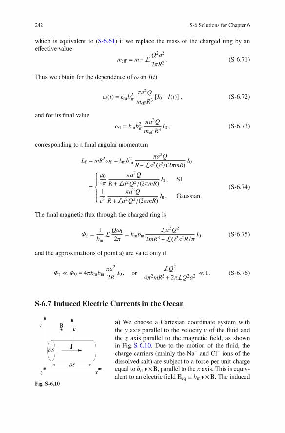
242 S-6 Solutions for Chapter 6
which is equivalent to (S-6.61) if we replace the mass of the charged ring by an
effective value
meff = m+L Q2a2
2πR2. (S-6.71)
Thus we obtain for the dependence of ω on I(t)
ω(t) = kmb2m
πa2Q
meffR3[I0− I(t)] , (S-6.72)
and for its final value
ωf = kmb2m
πa2Q
meffR3I0 , (S-6.73)
corresponding to a final angular momentum
Lf = mR2ωf = kmb2m
πa2Q
R+La2Q2/(2πmR)I0
=
⎧⎪⎪⎪⎪⎪⎪⎨⎪⎪⎪⎪⎪⎪⎩
μ0
4π
πa2Q
R+La2Q2/(2πmR)I0 , SI,
1
c3
πa2Q
R+La2Q2/(2πmR)I0 , Gaussian.
(S-6.74)
The final magnetic flux through the charged ring is
Φf =1
bmL Qωf
2π= kmbm
La2Q2
2mR3+LQ2a2R/πI0 , (S-6.75)
and the approximations of point a) are valid only if
Φf ≪Φ0 = 4πkmbmπa2
2RI0 , or
LQ2
4π2mR2+2πLQ2a2≪ 1. (S-6.76)
S-6.7 Induced Electric Currents in the Ocean
S
B
J
y
xz
Fig. S-6.10
a) We choose a Cartesian coordinate system with
the y axis parallel to the velocity v of the fluid and
the z axis parallel to the magnetic field, as shown
in Fig. S-6.10. Due to the motion of the fluid, the
charge carriers (mainly the Na+ and Cl− ions of the
dissolved salt) are subject to a force per unit charge
equal to bm v×B, parallel to the x axis. This is equiv-
alent to an electric field Eeq ≡ bm v×B. The induced

S-6.7 Induced Electric Currents in the Ocean 243
current density is thus
J = σEeq = bmσv×B. (S-6.77)
b) Inserting the typical values given in the text into (S-6.77) we obtain
J ≃
⎧⎪⎪⎪⎨⎪⎪⎪⎩4×1×5×10−5 = 2×10⁻⁴ A/m2 , SI,
3.6×1010× 100
c×0.5 = 60statA/cm2 , Gaussian.
(S-6.78)
c) We evaluate the force on a fluid element of cylindrical shape, with area of the
bases δS and height |δℓ|, where ℓ is parallel to J and to the x axis. The current
intensity in the cylinder is I = JδS , and the force acting on it is thus δF= bmIδℓ×B=
−bmBJ δS δℓ y = −bmBJ δV y, where δV is the volume of the cylinder. The mass
of the cylinder is δm = ρδV, with ρ = 103 kg/m3 (1 g/cm3 in Gaussian units), for
water. Both v and δF are parallel to the y direction, and the equation of motion can
be written in scalar form
δmdv
dt= δF . (S-6.79)
Replacing the values of δm and δF we obtain
ρδV dv
dt= −bmBJ δV ,
ρdv
dt= −b2
mB2σv , (S-6.80)
where we have divided both sides by δV and replaced J by its expression (S-6.77).
The solution is a decreasing exponential v = v0e−t/τ with a time constant
τ =ρ
σb2mB2
≃ 1011 s ≃ 3×10³ yr . (S-6.81)
S-6.8 A Magnetized Sphere as Unipolar Motor
a
I
M
rB
df
B O
Pz
d
Fig. S-6.11
a) We recall from Problem 5.10 that the magnetic
field inside a uniformly magnetized sphere is uni-
form and equals
B =8π
3
km
bmM =
⎧⎪⎪⎪⎪⎨⎪⎪⎪⎪⎩
2μ0
3M , SI,
8π
3M , Gaussian.
(S-6.82)

244 S-6 Solutions for Chapter 6
Outside of the sphere we have the same magnetic field that would be generated by
a magnetic dipole of moment m =M4πa3/3, located at the center of the sphere.
When an electric current I flows in the circuit, the magnetic force on an element
dℓ of the “meridian” wire BP is df = Idℓ×B, directed out of paper in Fig. S-6.11.
Since the component of B perpendicular to dℓ is continuous across the surface of
the sphere, there is no ambiguity. The torque dτ on the wire element dℓ is
dτ = r×df = Ir× (dℓ×B) = z IasinθadθBcosθ
= z Ia2Bcosθ sinθdθ , (S-6.83)
where r is the distance of dℓ form the rotation axis of the sphere (r = asinθ), and
we have used adθ = dℓ. The total torque on the meridian wire BP is thus
τ =
∫dτ = z Ia2B
∫ π/2
0
sinθcosθdθ = z1
2Ia2B , (S-6.84)
I
+
−
M
R
V
I
d
dfB
B
A P
Fig. S-6.12
while the torque on the current-carrying portion AB
of the “equatorial” wire is zero, because the mag-
netic force is radial, as shown in Fig. S-6.12. Thus,
(S-6.84) is the total torque on the sphere.
b) When the sphere rotates, the total electromotive
force Etot in the circuit is the sum of the electromo-
tive force of the voltage source and the electromotive
force Erot due to the rotation of the of the wires
Etot = V +Erot = V −bmdΦ
dt, (S-6.85)
R
V
D
+
−P
BA
M
I
C
EO
Fig. S-6.13
whereΦ is the flux of the magnetic field through any
surface bounded by the closed path ABPCDEA in
Fig. S-6.13. Lines PC, CD, DE and EA are copla-
nar lines, lying on a plane containing also the rota-
tion axis OP of the sphere and the meridian arc PA,
while AB is an equatorial arc, and BP a meridian arc,
both lying on the surface of the sphere. The flux of
B through any surface bounded by the closed path
ABPCDEA is the same, because ∇ ·B = 0. For sim-
plicity, we choose a surface comprising two parts:
1. the planar surface PCDEA, its perimeter being closed by the arc AP, through
which the flux is zero, and
2. the spherical polar triangle PAB shaded in Fig. S-6.13.

S-6.8 A Magnetized Sphere as Unipolar Motor 245
The flux through PAB can be easily calculated remembering that the flux of B
through any closed surface is zero. Consider the closed surface formed by PAB
and the three circular sectors OAP, OBP and OAB. The flux through OAP and OBP
is zero, thus the flux ΦPAB through PAB and the flux ΦOAB through OAB must be
equal (ΦOAB must be taken with the minus sign when evaluating its contribution
to the flux through the total closed surface, since the magnetic field enters through
OAB and exits through PAB), and we have
ΦPAB =ΦOAB =1
2Ba2φ, (S-6.86)
where φ is the angle AOB. We thus have
Etot = V −bmdΦ
dt= V −bm
Ba2
2
dφ
dt= V −bm
Ba2
2ω, (S-6.87)
and the current flowing in the circuit is
I =Etot
R=
1
R
(V −bm
Ba2
2ω
). (S-6.88)
The torque on the sphere is zero when I = 0, thus the terminal angular velocity of
the sphere is
ωt =2V
bmBa2=
⎧⎪⎪⎪⎪⎪⎨⎪⎪⎪⎪⎪⎩
2V
Ba2, SI,
2V
Ba2c , Gaussian,
(S-6.89)
independent of the moment of inertia of the sphere I and of the resistance R of the
circuit. The equation of motion for the sphere is
I dω
dt= τ =
1
2Ba2I =
Ba2
2R
(V −bm
Ba2
2ω
), (S-6.90)
which, using (S-6.89), can be rewritten as
I dω
dt= −bm
(Ba2)2
4IR(ω− 2V
bmBa2) ≡= −1
τ(ω−ωt) , (S-6.91)
where
τ =4IR
bm(Ba2)2. (S-6.92)
Assuming that the sphere is at rest at t = 0, the solution is
ω(t) = ωt
(1− e−t/τ
). (S-6.93)

246 S-6 Solutions for Chapter 6
S-6.9 Induction Heating
a) When the displacement current is neglected, (6.5) can be written as
∇×B = 4πkm(Jf +Jm) = 4πkm μr Jf , (S-6.94)
where Jf is the free current density and Jm is the magnetization current density.
Now, using (A.12),
∇× (∇×B) = −∇2B+∇(∇ ·B) = 4πkmμr∇×Jf , (S-6.95)
and recalling that ∇ ·B = 0 and Jf = σE we obtain
−∇2B = 4πkmμrσ∇×E . (S-6.96)
Finally, using ∇×E = −bm ∂tB we have
∂tB = (4πkmbm μrσ)−1∇2B ≡ α∇2B , (S-6.97)
where
α =1
4πkmbm μrσ=
⎧⎪⎪⎪⎪⎪⎪⎨⎪⎪⎪⎪⎪⎪⎩
1
μ0μrσ, SI,
c2
4πμrσ, Gaussian.
(S-6.98)
b) The tangential component of the auxiliary vector H must be continuous through
the x = 0 plane, thus, the tangential component of B/μr must be continuous. In the
vacuum half-space (x < 0) we have B = y B0 cos(ωt), correspondingly, the field at
x = 0+ (just inside our medium) is
B(0+, t) = yμrB0 cos(ωt) . (S-6.99)
In one dimension, (6.6) is rewritten
∂tB = α∂2xB , (S-6.100)
and, as an educated guess, we look for a solution of the form B(x, t)=Re[B(x)e−iωt
].
The differential equation for the time-independent function B(x) is
− iωB = α∂2xB , (S-6.101)
and we look for an exponential solution of the form B(x) = B(0)eγx, with B(0) and
γ two constants to be determined. The boundary condition gives B(0) = μrB0, and,
by substituting into (S-6.101), we have
− iωμrB0 eγx = αγ2μrB0 eγx , (S-6.102)

S-6.9 Induction Heating 247
which leads to αγ2 = −iω, so that
γ = ±√−iω
α= ±1− i√
2
√ω
α= ±(1− i)
1
ℓs(S-6.103)
where (1− i)/√
2 =√−i, and the quantity
ℓs =
√2α
ω=
√2
4πkmbmμrσω=
⎧⎪⎪⎪⎪⎪⎪⎪⎪⎨⎪⎪⎪⎪⎪⎪⎪⎪⎩
√2
μ0μrσω, SI,
√c2
2πμrσω, Gaussian,
(S-6.104)
which has the dimension of a length, is called the (resistive) skin depth. We dis-
regard the positive value of γ, which would lead to a magnetic field exponentially
increasing with distance into the material, and obtain
B = y Re[μrB0 e−(1−i)x/ℓs−iωt
]= yμrB0 e−x/ℓs cos
(x
ℓs−ωt
). (S-6.105)
Thus the magnetic field decreases exponentially with distance into the material, with
a decay length ℓs. A slab of our material can be considered as semi-infinite if its
depth is much larger than ℓs.
c) The electric field E(x) inside the material can be evaluated from ∇×E = −bm ∂tB.
Assuming E(x, t) = Re[E(x)e−iωt
]we have
(∇×E)y = −∂x Re[Ez(x)e−iωt
],
∂tB = Re[−iωμrB0 e−(1−i)x/ℓs−iωt
], (S-6.106)
thus E(x, t) = z Re[Ez(x)e−iωt
], with ∂xEz = −ibmωμrB0 e−(1−i)x/ℓs . Integrating with
respect to x we obtain
Ez =i
1− ibmωμrℓsB0 e−(1−i)x/ℓs = −1− i
2bmωμrℓsB0 e−(1−i)x/ℓs . (S-6.107)
The dissipated power per unit volume, due to the free currents only, is thus
〈Jf ·E〉 =σ
2
∣∣∣Ez
∣∣∣2 = σ4
b2m μ
2rω
2ℓ2s B20e−2x/ℓs =
σ
4b2
m
2μ2rω
2B20
4πkmbmμrσωe−2x/ℓs
= bm
μrωB20
8πkme−2x/ℓs =
⎧⎪⎪⎪⎪⎪⎪⎪⎨⎪⎪⎪⎪⎪⎪⎪⎩
μrωB20
2μ0e−2x/ℓs , SI,
μrωB20
32π2e−2x/ℓs , Gaussian,
(S-6.108)

248 S-6 Solutions for Chapter 6
where we have substituted (S-6.104) for ℓs in the fraction. The total dissipated power
per unit surface of the slab is
∫ ∞
0
〈Jf ·E〉dx = bm
μrωB20
16πkmℓs =
B20
16π
√bmμrω
2kmσ. (S-6.109)
One might wonder if there is also a contribution of the magnetization volume and
surface current densities, Jm and Km, to the dissipated power. In the presence of the
magnetic field (S-6.105), our medium of relative magnetic permeability μr acquires
a magnetization M
M =bm
4πkm
μr−1
μrB = y
bm
4πkm(μr−1)Re
[B0 e−(1−i)x/ℓs−iωt
], (S-6.110)
which corresponds to
Jm =1
bm∇×M . (S-6.111)
Taking the symmetry of the problem into account, and introducing the complex
amplitudes Jm and Jm z such that Jm = Re(Jm e−iωt
)= z Re
(Jm ze−iωt
), we have
Jm z =μr−1
4πkmμr∂xB = −μr−1
4πkm
1− i
ℓsB0 e−(1−i)x/ℓs . (S-6.112)
The corresponding power per unit volume is
〈Jm ·E〉 =1
2Re
(Jm zE∗z
)= bm (μr−1)
μrωB20
8πkme−2x/ℓs = (μr −1)〈Jf ·E〉 , (S-6.113)
and the total power per unit surface is
∫ ∞
0
〈Jm ·E〉dx = (μr−1)
∫ ∞
0
〈Jf ·E〉dx = bm (μr−1)μrωB2
0
16πkmℓs . (S-6.114)
However, we also have a surface magnetization current density Km flowing on the
x = 0 plane, given by
Km =1
bmM(0+)× n = z
μr −1
4πkmRe
(B0 e−iωt
)= z Km zcos(ωt) , (S-6.115)
where n = −x is the outward-pointing unit vector on the x = 0 boundary plane. This
surface current density corresponds to a power per unit surface
〈Km(t) ·E(0, t)〉 = 1
2Re
[Km zEz(0)
]= −bm(μr−1)
μrωB20
16πkmℓs , (S-6.116)
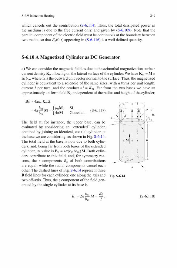
S-6.9 Induction Heating 249
which cancels out the contribution (S-6.114). Thus, the total dissipated power in
the medium is due to the free current only, and given by (S-6.109). Note that the
parallel component of the electric field must be continuous at the boundary between
two media, so that Ez(0, t) appearing in (S-6.116) is a well defined quantity.
S-6.10 A Magnetized Cylinder as DC Generator
a) We can consider the magnetic field as due to the azimuthal magnetization surface
current density Km, flowing on the lateral surface of the cylinder. We have Km =M×n/bm, where n is the outward unit vector normal to the surface. Thus, the magnetized
cylinder is equivalent to a solenoid of the same sizes, with n turns per unit length,
current I per turn, and the product nI = Km. Far from the two bases we have an
approximately uniform field B0, independent of the radius and height of the cylinder,
h
a
M
Bz
B0
Fig. S-6.14
B0 ≃ 4πkmKm z
= 4πkm
bmM =
μ0M , SI,
4πM , Gaussian.(S-6.117)
The field at, for instance, the upper base, can be
evaluated by considering an “extended” cylinder,
obtained by joining an identical, coaxial cylinder, at
the base we are considering, as shown in Fig. S-6.14.
The total field at the base is now due to both cylin-
ders, and, being far from both bases of the extended
cylinder, its value is B0 ≃ 4π(km/bm)M. Both cylin-
ders contribute to this field, and, for symmetry rea-
sons, the z components Bz of both contributions
are equal, while the radial components cancel each
other. The dashed lines of Fig. S-6.14 represent three
B field lines for each cylinder, one along the axis and
two off-axis. Thus, the z component of the field gen-
erated by the single cylinder at its base is
Bz = 2πkm
bmM =
B0
2. (S-6.118)

250 S-6 Solutions for Chapter 6
h
a
V
E
M
F
G
D
C
AH
B O
Fig. S-6.15
b) We apply Faraday’s law of induction to the
flux of the magnetic field through the closed path
AEFGBCDA, represented by the thick line in
Fig. S-6.15. Points A, E, F, G, and B are fixed in the
laboratory frame, while points C and D rotate with
the magnetized cylinder. We have
E = −bmdΦ
dt, (S-6.119)
where E is the electromotive force around the closed
path, measured by the voltmeter V , and Φ is the flux
of the magnetic field through any surface bounded
by the closed path. We choose a surface consisting
of three parts:
1. the plane surface bounded by the path AEFGBHA, fixed in the laboratory frame,
through which the flux of B is zero;
2. the surface bounded by the path BCDHB, lying on the lateral surface of the
cylinder; and
3. the circular sector AHD on the upper base, where points A and H are fixed, while
point D is rotating.
The flux of B through the two surfaces BCDH and AHD can be calculated analo-
gously to the flux through the polar spherical triangle PAB of Fig. S-6.13, Problem
6.8. We consider the closed surface comprising, in addition to BCDH and AHD, the
circular sector OBC and the two rectangles COAD and BOAH. The flux must be
zero through the total closed surface, and is zero through the two rectangles because
B is parallel to their surfaces. Thus we have
ΦAHD+ΦBCDH +ΦOBC = 0 , (S-6.120)
and
ΦAHD+ΦBCDH = −ΦOBC =1
2B0 a2φ, (S-6.121)
where φ is the angle BOC = HAD, and the sign accounts for the fact that the mag-
netic field is entering the closed surface through OBC. The electromotive force is
E = −bmdΦ
dt= −bm
1
2B0 a2 dφ
dt= 2πkmMa2ω =
⎧⎪⎪⎪⎪⎨⎪⎪⎪⎪⎩
μ0
2Ma2ω, SI,
2π
cMa2ω, Gaussian.
(S-6.122)
The same result can be obtained by evaluating the electromotive force E as the
integral of bm(v×B) ·dℓ along the path AOB

S-6.10 A Magnetized Cylinder as DC Generator 251
E = bm
∫ O
A
(v×B) ·dℓ+bm
∫ B
O
(v×B) ·dℓ = bm
∫ a
O
ωrB0 dr
= bm1
2B0a2ω = 2πkmMa2ω, (S-6.123)
since v = 0 along the path AO, which lies on the rotation axis of the cylider.
S-6.11 The Faraday Disk and a Self-sustained Dynamo
a) The magnetic force on the each charge carrier of the rotating disk is qbmv×B,
where q is the charge of the carrier (−e for the electrons), and v = ω × r is the
velocity of a charge-carrier at a distance r from the rotation axis, at rest relative to
the disk. At equilibrium, carriers must be at rest relative to the disk, and the magnetic
force must be compensated by a static electric field E such that E+bm v×B= 0. This
corresponds to an electric potential drop V between the center and the circumference
of the disk
V = ϕ(a)−ϕ(0) = −∫ a
0
E ·dr = bm
∫ a
0
ωrBdr = bmωBa2
2. (S-6.124)
The rotating disk is thus a voltage source, known as a Faraday disk.
b) In the presence of the brush contacts at points O and A of Fig. 6.9, the electromo-
tive force E of he circuit equals the voltage drop V of (S-6.124). The total current I
circulating in the circuit is thus
I =ER= bm
ωBa2
2R. (S-6.125)
d
z
h
B
J × B
a
dr
J
I
A
Fig. S-6.16
The power dissipated in the circuit by Joule
heating is Pd = I2R=E2/R, and there must an
external a torque τext providing a mechanical
power Pm = τext ·ω = Pd in order to maintain
a rotation at constant angular velocity. Thus,
τext = zb2m
ωB2a4
4R. (S-6.126)
Alternatively, the external torque must com-
pensate the torque of the magnetic forces
on the disk. Since the current exits the disk
through the brush contact A, it is difficult to
make assumptions on the symmetry of the current density distribution. However, the
problem can be tackled as follows. The torque on an infinitesimal volume element,

252 S-6 Solutions for Chapter 6
r dφdr dz in cylindrical coordinates (Fig. S-6.16), is dτ = bm r× (J×B)r dφdr dz,
and the total magnetic torque on the disk is obtained by integrating dτ over the disk
volume
τB = bm
∫ a
0
dr
∫ h
0
dz
∫ 2π
0
r dφr× (J×B) . (S-6.127)
The vector triple product in (S-6.127) can be rewritten
r× (J×B) = J (r ·B)−B (r ·J) = −z BrJr , (S-6.128)
since (r ·B) = 0 because r and B are orthogonal to each other, and Jr is the r
R
Ir
hJ A
a
Fig. S-6.17
component of J. We further have
∫ h
0
dz
∫ 2π
0
r dφ Jr = I , (S-6.129)
independently of r, since the double
integral is the flux of J through a
lateral cylindrical surface of radius r
and height h, as shown in Fig. S-6.17.
Thus we have for the torque exerted
by the magnetic forces on the disk
τB = −zbm BI
∫ a
0
r dr , (S-6.130)
and finally, substituting (S-6.125) for I,
τb = −zbm BIa2
2= −zb2
m
ωB2a4
4R= −τext . (S-6.131)
c) If the disk acts as the current source for the solenoid we must have
B = 4πkm nI = 4πkmbm nωBa2
2R, (S-6.132)
from which we find that the frequency must be a function of the circuit parameters
ω =2R
4πkmbm na2=
⎧⎪⎪⎪⎪⎪⎨⎪⎪⎪⎪⎪⎩
2R
μ0na2, SI,
Rc2
2πna2, Gaussian,
(S-6.133)
independently of the intensity of the magnetic field B.

S-6.12 Mutual Induction Between Circular Loops 253
S-6.12 Mutual Induction Between Circular Loops
a) We can assume the magnetic field generated by the current I circulating in loop
B to be uniform and equal to B0 z = z2πkm I/b all over the surface of loop A, since
a≪ b. The angle between the axis of loop A and the z axis is θ = ωt, and the flux of
the magnetic field through the surface of loop A is
Φ = B0 πa2 cosωt =
2πkmI
bπa2 cosωt =
2π2a2kmI
bcosωt . (S-6.134)
Thus, according to Faraday’s law of induction, there is an induced electromotive
force E on loop A
E = −dΦ
dt=
2π2a2kmI
bωsinωt , (S-6.135)
and the current circulating in loop A is
IA =2π2a2kmI
Rbωsinωt . (S-6.136)
b) The power dissipated into Joule heating is
Pdiss = RI2A =
4π4a4ω2k2mI2
Rb2sin2ωt . (S-6.137)
c) The torque acting on loop A is τ = m×B0, where m = n IAπa2 is the magnetic
moment of loop A, and n is the unit vector perpendicular to its surface, directed so
that its tip sees IA circulating counterclockwise. Thus
τ =2π2a2kmI
Rbωsinωtπa2 2πkmI
bsinωt =
4π4a4ωk2mI2
Rb2sin2ωt , (S-6.138)
and the corresponding mechanical power is
Pmech = τ ·ω =4π4a4ω2k2
mI2
Rb2sin2ωt = Pdiss , (S-6.139)
and all the mechanical power needed to keep loop A rotating at constant angular
velocity is turned into Joule heating.
d) The flux through the surface of loop B of the magnetic field generated by the
current I circulating in loop A is
ΦB = MABI , (S-6.140)

254 S-6 Solutions for Chapter 6
where MAB is the coefficient of mutual induction between loop A and loop B. We
know that MAB = MBA, and from (S-6.134) we have
MAB = MBA =2π2a2km
bcosωt , (S-6.141)
thus
ΦB =2π2a2kmI
bcosωt , (S-6.142)
and
E = −dΦ
dt=
2π2a2kmI
bωsinωt , (S-6.143)
as (S-6.134) and (S-6.135) .
S-6.13 Mutual Induction between a Solenoid and a Loop
a) Neglecting boundary effects, the magnetic field inside the solenoid is uniform,
parallel to the solenoid axis z, and equal to
B = 4πkmnI z . (S-6.144)
Thus, its flux through the surface S of the rotating coil is
Φa(t) = B ·S(t) = 4πkmnIπa2 cosωt = 4π2a2kmnI cosωt = Msl(t) I , (S-6.145)
where
Msl(t) = 4π2a2kmncosωt (S-6.146)
is the coefficient of mutual inductance between solenoid and loop, time dependent
because the loop is rotating. The coefficient of mutual inductance is symmetric,
Msl = Mls, i.e., the inductance by the solenoid on the loop equals the inductance by
the loop on the solenoid, we shall use this property for the answer to point c).
b) The electromotive force acquired by the loop equals the rate of change of the
magnetic flux through it,
E = −dΦ
dt= 4π2a2kmnIωsinωt , (S-6.147)
and the current circulating in the loop is
Ia =4π2a2kmnIω
Rsinωt . (S-6.148)

S-6.13 Mutual Induction between a Solenoid and a Loop 255
The loop dissipates a power Pdiss due to Joule heating
Pdiss = RI2a =
(4π2a2kmnIω)2
Rsin2ωt . (S-6.149)
This power must be provided by the work of the torque τ applied to the loop in order
to keep it in rotation at constant angular velocity. The time-averaged power is
〈Pdiss〉 =(4π2a2kmnIω)2
2R, (S-6.150)
since⟨sin2ωt
⟩= 1/2.
c) The magnetic field generated by a magnetic dipole m is identical to the field
generated by a current-carrying loop of radius a and current Il such that bmπa2Il =m,
at distances r ≫ a from the center of the loop. The result of point a) is valid, in
particular, in the case a≪ b. In this case we can replace the magnetic dipole by a
loop, and use the symmetry property of the mutual-inductance coefficient. The flux
Φs generated by the dipole through the solenoid is thus
Φs = Mls(t) Il = 4π2a2kmnIl cosωt = 4πkm
bmnmcosωt . (S-6.151)
S-6.14 Skin Effect and Eddy Inductance in an Ohmic Wire
Assuming a very long, straight cylindrical wire, the problem has cylindrical sym-
metry. We choose a cylindrical coordinate system (r,φ,z) with the z axis along the
axis of the wire, and expect that the electric field inside the wire can be written as
E = z E(r, t) = z Re[E(r)eiωt
], (S-6.152)
where E(r) is the static complex amplitude associated to the electric field. We start
from the two Maxwell equations
∇×E = −bm ∂tB , ∇×B = 4πkm J+1
bmc2∂tE , (S-6.153)
where we have assumed εr = 1 and μr = 1 inside copper. If we substitute J = σE
into the second of (S-6.153) we obtain

256 S-6 Solutions for Chapter 6
∇×B = 4πkmσE+1
bmc2∂tE = 4πkmσE+ z
ω
bmc2Re
[iE(r)eiωt
]
=
⎧⎪⎪⎪⎪⎨⎪⎪⎪⎪⎩
μ0σE+ zω
c2Re
[iE(r)eiωt
], SI,
4πσ
cE+ z
ω
cRe
[iE(r)eiωt
], Gaussian.
(S-6.154)
In SI units, the conductivity of copper is σ = 5.96× 10⁷Ω−1m−1, and the product
μ0σc2 is
μ0σc2 = 6.77×10¹⁸ s−1 . (S-6.155)
Alternatively, in Gaussian units, the conductivity of copper is σ = 5.39× 10¹⁷ s−1
and the product 4πσ is 6.77× 10¹⁸ s−1. Thus the displacement current is negligible
compared to the conduction current J for frequencies ν = ω/(2π)≪ 1018 Hz, i.e.,
up to the ultraviolet. In other words, the displacement current can be neglected
compared to the conduction current for all practical purposes in good conductors,
and we can rewrite the second of (S-6.153) simply as ∇×B = 4πkmσE. Evaluating
the curl of both sides of the first of (S-6.153) we have
∇× (∇×E) = −bm∂t(∇×B) = −4πkmbmσ∂tE , (S-6.156)
which, remembering that
∇× (∇×E) = ∇(∇ ·E)−∇2E , (S-6.157)
and assuming ∇ ·E = 0, turns into a diffusion equation for the electric field E
∇2E = 4πkmbmσ∂tE . (S-6.158)
Introducing our assumption (S-6.152), we have the following equation in cylindrical
coordinates for the complex amplitude E(r),
∇2E(r) =1
r∂r[r∂rE(r)] = iω4πkmbmσ E(r) (S-6.159)
or1
r∂r[r∂rE(r)] = i
2
δ2E(r) , (S-6.160)
where we have introduced the skin depth
δ =
√1
2πkmbmσω=
⎧⎪⎪⎪⎪⎪⎪⎨⎪⎪⎪⎪⎪⎪⎩
√2
μ0σω, SI,
c√
2πσω, Gaussian.
(S-6.161)

S-6.14 Skin Effect and Eddy Inductance in an Ohmic Wire 257
Equation (S-6.160), multiplied by r2, is Bessel’s differential equation with n = 0.
However, in this context, we prefer to find the approximate solutions for the two
limiting cases δ≫ r0 and δ≪ r0, where r0 is the radius of the wire. For the weak
skin effect, i.e., for δ≫ r0, we write the solution of (S-6.160) as a Taylor series
E(r) = E0
∞∑
n=0
an
(r
δ
)n
(S-6.162)
which, substituted into the left-hand side of (S-6.160) gives
1
r∂r[r∂rE(r)] =
1
r∂r
⎡⎢⎢⎢⎢⎢⎢⎣rE0
∞∑
n=0
annrn−1
δn
⎤⎥⎥⎥⎥⎥⎥⎦ =1
rE0 ∂r
∞∑
n=0
annrn
δn
=1
rE0
∞∑
n=0
ann2rn−1
δn= E0
∞∑
n=0
ann2rn−2
δn, (S-6.163)
while the right-hand side is
i2
δ2E(r) = 2i E0
∞∑
n=0
anrn
δn+2. (S-6.164)
Comparing the coefficients of the same powers of r in (S-6.163) and (S-6.164) we
obtain the recurrence relation
an+2 =2i
(n+2)2an , (S-6.165)
which leads to
a2n =in
2n(n!)2and a2n+1 = 0 , (S-6.166)
for all n ≥ 0 and n ∈ N. We thus have
E(r) = E0
∞∑
n=0
in
2n(n!)2
(r
δ
)2n
= E0
[1+
i
2
r2
δ2− 1
16
r4
δ4− i
48
r6
δ6+ · · ·+ in
2n(n!)2
r2n
δ2n+ . . .
]. (S-6.167)
The complex amplitude I associated to the total current through the wire is
258 S-6 Solutions for Chapter 6
I =
∫ r0
0
J2πr dr = 2πσ
∫ r0
0
E(r)r dr
= 2πσE0
∫r0
0
[1+
i
2
r2
δ2− 1
16
r4
δ4− i
48
r6
δ6+ · · ·+ in
2n(n!)2
r2n
δ2n+ . . .
]r dr
= 2πσE0
⎡⎢⎢⎢⎢⎢⎣r2
0
2+
i
8
r40
δ2− 1
96
r60
δ4− i
2304
r80
δ6+ · · ·+ in
2n(n!)2(2n+2)
r2n+20
δ2n
⎤⎥⎥⎥⎥⎥⎦
= πr20σE0
⎡⎢⎢⎢⎢⎢⎣1+i
4
r20
δ2− 1
48
r40
δ4− i
1152
r60
δ6+ · · ·+ in
2n(n+1)!n!
r2n0
δ2n+ . . .
⎤⎥⎥⎥⎥⎥⎦ . (S-6.168)
We can define the impedance per unit length of the wire, Zℓ = Rℓ + iωLℓ (where Rℓis the resistance per unit length, and Lℓ the self-inductance per unit length), as the
ratio of the electric field at the wire surface to the total current through the wire,
i.e., as
Zℓ =1
πr20σ
[1+
i
2
(r0
δ
)2
− 1
16
(r0
δ
)4
− i
48
(r0
δ
)6
+ . . .
]
︸︷︷︸A
×[1+
i
4
(r0
δ
)2
− 1
48
(r0
δ
)4
− i
1152
(r0
δ
)6
+ . . .
]−1
︸︷︷︸B−1
, (S-6.169)
where A and B are Taylor expansions in even powers of r0/δ≪ 1, which we have
truncated at the 6th order. The first four expansion coefficients of B−1, i.e., 1, b1, b2,
and b3,
B−1 =
[1+b1
(r0
δ
)2
+b2
(r0
δ
)4
+b3
(r0
δ
)6
+ . . .
], (S-6.170)
can be evaluated by requiring that the product BB−1 equals 1 with a remainder of
the order of (r0/δ)8, i.e.,
1 = BB−1 ≃[1+
i
4
(r0
δ
)2
− 1
48
(r0
δ
)4
− i
1152
(r0
δ
)6
+ . . .
]
×[1+b1
(r0
δ
)2
+b2
(r0
δ
)4
+b3
(r0
δ
)6
+ . . .
](S-6.171)
leading to
b1 = −i
4, b2 = −
1
24, and b3 =
7i
1152(S-6.172)

S-6.14 Skin Effect and Eddy Inductance in an Ohmic Wire 259
Thus we have for Zℓ
Zℓ ≃1
πr20σ
[1+
i
2
(r0
δ
)2
− 1
16
(r0
δ
)4
− i
48
(r0
δ
)6
+ . . .
]
×[1− i
4
(r0
δ
)2
− 1
24
(r0
δ
)4
+7i
1152
(r0
δ
)6
+ . . .
]
≃ 1
πr20σ
[1+
i
4
(r0
δ
)2
+1
48
(r0
δ
)4
− i23
1152
(r0
δ
)6
+ . . .
]. (S-6.173)
The zeroth-order term of the expansion,
R(0)
ℓ=
1
πr20σ, (S-6.174)
is simply the direct-current resistance per unit length of the wire. The third term
R(1)
ℓ=
r20
48πσδ4=
k2mb2
mπr20σω2
12=
⎧⎪⎪⎪⎪⎪⎪⎨⎪⎪⎪⎪⎪⎪⎩
μ20πr2
0σω2
192, SI,
πr20σω2
12c4, Gaussian
(S-6.175)
is the lowest order contribution of the weak skin effect to the resistance increase.
The second-order term of the expansion can be interpreted as
i
4πr20σ
(r0
δ
)2
= iωL(0)
ℓ, (S-6.176)
leading to
L(0)
ℓ=
1
4πσωr20
(r0
δ
)2
=1
2kmbm =
⎧⎪⎪⎪⎪⎨⎪⎪⎪⎪⎩
μ0
8π, SI,
1
2c2, Gaussian,
(S-6.177)
r
a
z
x
Fig. S-6.18
which is the DC self-inductance per unit length of a
straight cylindrical wire, while the sixth-order term
is the lowest order contribution of the weak skin-
effect to the self-inductance of the cylindrical wire.
Thus, at the low-frequency limit, the current depends
on the radial coordinate, but no true skin effect
is observed. According to (S-6.168), the current is
actually stronger on the axis of the wire than at its
surface.
260 S-6 Solutions for Chapter 6
Things are different at the high-frequency limit. As the frequency increases, the
skin depth becomes progressively smaller. When δ≪ a, the fields will be varying in
space on a distance much smaller than the wire radius, so that we expect the effect
of the curvature to be negligible. For a strong skin effect, i.e., for δ≪ a, the electric
field is significantly different from zero only close to the wire surface. Thus, we
introduce the variable x = a−r, shown in Fig. S-6.18, and assume r ≃ a in (S-6.160).
Using ∂r = −∂x we get
∂2xE = i
2
δ2E . (S-6.178)
Substituting E = E0 eαx, we have
α = ±√
i2
δ2= ±1+ i
δ, (S-6.179)
and the solution corresponding to a field decreasing for increasing x (increasing
depth into the wire) is
E ≃ E0 e−x/δ e−ix/δ = E0 e−(a−r)/δ e−i(a−r)/δ , (S-6.180)
where E0 eiωt is the electric field at the wire surface. The complex amplitude corre-sponding to the total current current through the wire is thus
I =
∫ a
0
J 2πr dr = 2πσ
∫ a
0
E(r)r dr = 2πσE0
∫ a
0
e−(a−r)/δ e−i(a−r)/δ eiωtr dr
= 2πσE0e−a(1+i)/δ+iωt
∫ a
0
er(1+i)/δr dr . (S-6.181)
Remembering that ∫xeaxdx = eax
(x
a− 1
a2
), (S-6.182)
and neglecting terms in δ2, we obtain finally
I = πaδσ(1− i) E0 . (S-6.183)
The impedance per unit length of the wire, Zℓ, can again be defined as
Zℓ = Rℓ + iXℓ =E0
I=
1
πaδσ(1− i)=
1
2πaδσ+
i
2πaδσ, (S-6.184)
so that the magnitudes of the resistance per unit length Rℓ, and of the reactance per
unit length Xℓ, are equal at the high frequency limit:
Rℓ = Xℓ =1
2πaδσ. (S-6.185)

S-6.14 Skin Effect and Eddy Inductance in an Ohmic Wire 261
The value of Rℓ shows that the current actually flows through a thin annulus close
to the surface (the “skin” of the wire), of width δ and approximate area 2πaδ. The
reactance per unit length can be considered as due to a self-inductance per unit
length Lℓ, according to Xℓ = ωLℓ, with
Lℓ =1
2πaδσω=
√kmbm
2πa2σω=
⎧⎪⎪⎪⎪⎪⎪⎪⎨⎪⎪⎪⎪⎪⎪⎪⎩
√μ0
8π2a2σω, SI,
√1
2πc2a2σω, Gaussian.
(S-6.186)
S-6.15 Magnetic Pressure and Pinch Effect for a Surface Current
a) We use a cylindrical coordinate system (r,φ,z), with the cylinder axis as z axis.
The field lines of B are circles around the z axis because of symmetry. Thus, Bφ(r)
is the only nonzero component of B. According to Ampere’s law we have
Bφ(r) =
⎧⎪⎪⎨⎪⎪⎩0 , r < a ,
2kmI
r= 4πkm K
a
r, r > a .
(S-6.187)
b) First approach (heuristic). The current dI flowing in an infinitesimal surface strip
parallel to z, of width adφ, is dI = Kadφ. The force df exerted by an azimuthal
magnetic field B ≡ (0,Bφ,0) on an infinitesimal strip portion of length dz is
df = bm dzdI z×B = −bmKaBφ dφdz r , (S-6.188)
directed towards the axis, i.e., so to shrink the conducting surface (pinch effect).
However, here we must remember that Bφ(r) is discontinuous at the cylinder sur-
face, being zero inside. Therefore, we replace the value of Bφ in (S-6.188) by its
“average” value Baverφ= [Bφ(a
+)−Bφ(a−)]/2 = 2πkm K (the point is the same as for
the calculation of electrostatic pressure on a surface charge layer). Thus, the absolute
value of the force acting on an infinitesimal area dS = adφdz is
|d f | = 2πkmbmK2 dS =
⎧⎪⎪⎪⎪⎨⎪⎪⎪⎪⎩
μ0
2K2 dS , SI
2π
c2K2 dS , Gaussian ,
(S-6.189)

262 S-6 Solutions for Chapter 6
and the magnetic pressure on the surface is
P =|d f |dS= 2πkmbmK2 = kmbm
I2
2πa2=
⎧⎪⎪⎪⎪⎪⎪⎨⎪⎪⎪⎪⎪⎪⎩
μ0I2
2(2πa)2, SI
1
c2
I2
2πa2, Gaussian.
(S-6.190)
Second method (rigorous). The magnetic force per infinitesimal volume d3r,
where a current density J is flowing in the presence of a magnetic field B, is
d3f = bm J×Bd3r . (S-6.191)
Due to the symmetry of our problem, the term (B · ∇)B appearing in (6.7) is
(B · ∇)B =
(Bφ
1
r∂φ
)B = 0 , (S-6.192)
where we have used the gradient components in cylindrical coordinates of Table
A.1, and the fact that the only nonzero component of B, i.e., Bφ, is independent of
φ. The infinitesimal volume element in cylindrical coordinates is d3r = r dr dφdz,
thus
z
d
a −a +
dz
r
Fig. S-6.19
d3f = −rbm
8πkm
[∂rB2
φ(r)]
r dr dφdz . (S-6.193)
Now we integrate (S-6.193) with respect to dr
between r = a− ε and a+ ε, obtaining the force d2f
acting on the small shaded volume of Fig. S-6.19,
delimited by the two cylindrical surfaces r = a− εand r = a+ ε, with infinitesimal azimuthal aperture
dφ, and longitudinal length dz. Integrating by parts
we have
∫ a+ε
a−ε
[∂rB2
φ(r)]r dr =
[rB2φ(r)
]a+ε
a−ε−∫ a+ε
a−εB2φ(r)dr , (S-6.194)
At the limit ε → 0, the first term on the right-hand side equals B2φ(a+), because
B2φ(r) = 0 for r < a. At the same limit ε→ 0, the integral on the right-hand side
approaches zero because, according to the mean-value theorem, it equals 2εB2φ(r),
with r some value in the range (a−ε,a+ε). We thus have
d2f = −rbm
8πkmB2φ(a+)adφdz . (S-6.195)

S-6.15 Magnetic Pressure and Pinch Effect for a Surface Current 263
where adφdz is the infinitesimal surface element on which d2f is acting. The pres-
sure is thus
P =bm
8πkmB2φ(a+) =
bm
8πkm
(4πkm K)2 = 2πbmkmK2, (S-6.196)
in agreement with (S-6.190). Now we prove (6.7):
4πkm(J×B)i = [(∇×B)×B]i = εi jk
(ε jlm
∂Bm
∂xl
)Bk = εi jkε jlm
∂Bm
∂xl
Bk
= (δklδim−δkmδil) Bk
∂Bm
∂xl
= Bk
∂Bi
∂xk
−Bk
∂Bk
∂xi
= (B×∇)Bi−1
2
∂(BkBk)
∂xi
= (B×∇)Bi−1
2∇iB
2 , (S-6.197)
where the subscripts i, j,k, l,m range from 1 to 3, and x1,2,3 = x,y,z, respectively.
The symbol εi jk is the Levi-Civita symbol, defined by εi jk = 1 if (i, j,k) is a cyclic
permutation of (1,2,3), εi, j,k = −1 if (i, j,k) is an anticyclic permutation of (1,2,3),
and εi, j,k = 0 if at least two of the subscripts (i, j,k) are equal.
c) The magnetic energy ∆UM stored in the infinite layer between z and z+∆z equals
the volume integral
∆UM =
∫
layer
uM d3r =
∫
layer
bm
8πkmB2(r)d3r
= 2π∆z
∫ ∞
a
bm
8πkmB2φ(r)r dr , (S-6.198)
which, involving the integral∫ ∞
ar−1dr, is infinite. However, if the radius of the
cylinder increases by da, the integrand does not change for r > a+ da, while the
integration (Fig. S-6.20) volume decreases. Correspondingly, the (infinite) value of
the integral decreases by the finite value
K B
a
um
z
daz z
z
z
Fig. S-6.20
d(∆UM) = −∆zbm
8πkmB2φ(a+)2πada .
(S-6.199)
Thus, an expansion of the current
carrying surface leads to a decrease
of the magnetic energy. If the sys-
tem were isolated, the force df acting
on the surface element dS = adφdz
would be directed radially outwards,
leading to an expansion of the cylinder. However, the system is not isolated, because
a current source is required to keep the current surface density K constant. An
increase of the radius da leads to a decrease of the magnetic flux in the layer equal

264 S-6 Solutions for Chapter 6
to d(∆Φ) = Bφ(a+)∆zda (see figure), which, in turn, implies the appearance of an
electromotive force ∆E. In fact, in order to keep K constant during the time inter-
val dt in which the cylinder radius increases by da, the source must provide to the
layer the energy d(∆Usource), that compensates the work d(∆W) = ∆E I dt done by
the electromotive force ∆E = −bm d(∆Φ)/dt, so that
d(∆Usource) = −bmI d(∆Φ) = 2πbmaKBφ(a+)∆zda
= bm 2πa1
4πkmB2φ(a+)∆zda = −2d(∆Um) . (S-6.200)
Thus, the total energy balance for the layer is given by
d(∆Utot) = d(∆Usource)+d(∆Um) = −d(∆Um) , (S-6.201)
and the force per unit surface is
P = − 1
2πa∆z
d(∆Utot)
da= +
1
2πa∆z
d(∆Um)
da, (S-6.202)
in agreement with (S-6.190).
S-6.16 Magnetic Pressure on a Solenoid
a) The magnetic force df on an infinitesimal coil arc of length dℓ, carrying a current
I, is
df = bm I dℓ×B . (S-6.203)
Thus, the force dF on the surface element dS = dℓ×dz of the solenoid, of width
dℓ, is
dF = bm IBndℓ×dz = bm IBndS , (S-6.204)
since the surface element comprises ndz coil arcs, each of length dℓ. The force dF
is directed towards the exterior of the solenoid, and the solenoid tends to expand
radially.
The magnetic field B is discontinuous at the surface of the solenoid, due to the
presence of the electric current in the coils. At the limit of an infinitely long solenoid
we have
B = B0 = 4πkmnI z =
⎧⎪⎪⎪⎨⎪⎪⎪⎩
μ0nI z , SI,
4π
cnIz , Gaussian,
(S-6.205)

S-6.16 Magnetic Pressure on a Solenoid 265
B
df
d
Ia
Fig. S-6.21
inside, where z is the unit vector along the solenoid
axis, and B = 0 outside. Thus we substitute the aver-
age value
B(a+)+B(a−)
2=
B0
2= 2πkm nI
for B in (S-6.204), obtaining
dF = 2πbmkm n2I2dS . (S-6.206)
The pressure P on the solenoid surface is obtained by dividing dF by dS , thus
P =dF
dS= 2πbmkm n2I2 =
bmB20
8πkm=
⎧⎪⎪⎪⎪⎪⎪⎨⎪⎪⎪⎪⎪⎪⎩
μ0
2n2I2 =
B20
2μ0, SI,
2πn2I2 =B2
0
8π, Gaussian.
(S-6.207)
b) The magnetic energy of the solenoid can be written in terms of the magnetic
energy density uM associated to the magnetic field B0
uM =bm
8πkmB2
0 =
⎧⎪⎪⎪⎪⎪⎪⎨⎪⎪⎪⎪⎪⎪⎩
B20
2μ0, SI,
B20
8π, Gaussian.
(S-6.208)
Neglecting the boundary effects, we obtain the total magnetic energy of the solenoid
UM by multiplying uM by the solenoid volume
UM = πa2huM =
a2hbmB20
8km= 2π2a2hbmkmn2I2 , (S-6.209)
thus, if the solenoid radius a increases by da the energy UM increases by
dUM = 4π2ahbmkmn2I2 da , (S-6.210)
while B0, given by (S-6.205), and thus uM, remain constant. This implies an increase
in the flux Φ of B0 through each coil of the solenoid
dΦ = 2πaB0 da = 8π2kmanI da , (S-6.211)
corresponding to a total electromotive force (the solenoid comprises hn coils)
E = −bmdΦ
dt= −bmkm 8π2ahn2I2 da
dt(S-6.212)

266 S-6 Solutions for Chapter 6
that must be compensated by the current source in order to keep I constant. The
work dWsource done by the current source is thus
dWsource = −EI dt = bmkm 8π2an2hI2 da . (S-6.213)
Thus the total energy of the system solenoid+current source changes by
dUtot = dUM−dWsource = −4π2ahbmkmn2I2 da . (S-6.214)
The pressure on the solenoid surface is P = −dUtot/dV , where V = πa2h is the vol-
ume of the solenoid. Thus
P = −dUtot
dV= − 1
2πah
dUtot
da= 2πbmkm n2I2 , (S-6.215)
in agreement with (S-6.207).
S-6.17 A Homopolar Motor
I
V
B
za
A
C
h
O
+
−
E
F
D
mag
net
b
l
Fig. S-6.22
The motor is schematized in the diagram of
Fig. S-6.22, that displays only one “half” of the cir-
cuit because of the symmetry of the problem. We use
cylindrical coordinates (r,φ,z) with the origin O at
the center of the cylindrical magnet, of radius b and
length l. The z axis coincides with the axes of the
magnet and of the cell, which here is represented by
the voltage source V . The circuit ACDEF is closed
by brush contacts (white arrows in the figure) to the
magnet at points A ≡ (0,φ, l/2) and F ≡ (b,φ,0), so
that the current I can flow through the conducting
magnet. The circuit is free to rotate around the z axis.
Let a > b and h be the horizontal and vertical sizes of
the circuit, respectively. We denote by B = B(r,φ,z)
the magnetic field generated by the magnet, indepen-
dent of φ, and with Bφ ≡ 0. Some field lines of B are
sketched in Fig. S-6.22. The magnetic field on the
z = 0 plane is parallel to the z axis, directed upwards for r < b, and downwards for
r > b. For simplicity, we approximate B(r,φ,0) = B0 z for r < b, with B0 independent
of r, even if this approximation is valid only for l≫ b.

S-6.17 A Homopolar Motor 267
B
A
O E
F
mag
net
b
l
d
I
I
z
dfr
Fig. S-6.23
The voltage source drives a current I through the
circuit. When the circuit is at rest we simply have
I = V/R, but, when the circuit rotates, we must take
into account the motion of the circuit in the presence
of the magnetic field. Since the magnetic field B lies
on the plane of the circuit, the force df = I dℓ×B on
an infinitesimal segment of the circuit dℓ is perpen-
dicular to the plane of the circuit (out of paper in the
case represented in Fig. S-6.23). The corresponding
infinitesimal torque relative to the z axis is thus
dτ = r×df = bm I r× (dℓ×B) , (S-6.216)
where r is the distance of dℓ from the z axis. The
torque dτ is always parallel (or antiparallel) to z, independently of the circuit ele-
ment dℓ we are considering. For the vector product dℓ×B we have
dℓ×B = −φBdℓ sinθ = −φBdℓcosψ
= −φB · ndℓ, (S-6.217)
B
d2
Fig. S-6.24
where θ is the angle between dℓ and B, n is the
unit vector perpendicular to dℓ, and ψ = θ − π/2 is
the angle between B and n, as shown in Fig. S-6.24.
Since r is perpendicular to φ (unit vectors of the cor-
responding cylindrical coordinates), we have for the
total torque acting on the circuit
τ = bm I
∫ F
A
r× (dℓ×B) = −zbm I
∫ F
A
B · nr dℓ .
(S-6.218)
The last integral of (S-6.218) can calculated, within our approximations, if we
first demonstrate that the line integral of B · nr around the closed path OCDEO of
Fig. S-6.22 is zero, i.e., that
∮B · nr dℓ =
∫ F
A
B · nr dℓ+
∫ O
F
B · nr dℓ+
∫ A
O
B · nr dℓ = 0 . (S-6.219)
First, we note that the integral along the whole OC path is zero, both because r is
zero, and because B is parallel to dℓ, thus perpendicular to n. Thus, the integral of
(S-6.219) becomes

268 S-6 Solutions for Chapter 6
∮B · nr dℓ =
∫ D
C
B · nr dr−∫ E
D
B · nr dz−∫ O
E
B · nr dr
=
∫ D
C
B · nr dr+
∫ D
E
B · nr dz+
∫ E
O
B · nr dr , (S-6.220)
since dℓ = dr along CD, dℓ = −dz along DE, and dℓ = −dr along EO.
I
B
A
C
O E
F
D
z
I
Fig. S-6.25
As a next step, we generate a cylinder by rotating
the CDEO path around thez axis, as in Fig. S-6.25.
The outgoing flux of the magnetic field B through
the total surface of the cylinder is
∫upperbase
B · ndS +
∫
lateralsurface
B · ndS +
∫
lowerbase
B · ndS = 0 ,
(S-6.221)since ∇ ·B = 0. Equation (S-6.221) can be rewritten
0 =
∫ a
0
B(r,φ,h) · n2πr dr+
∫ h
0
B(a,φ,z) · n2πr dz
+
∫ a
0
B(r,φ,0) · n2πr dr = 2π
∮B · nr dℓ , (S-6.222)
which demonstrates (S-6.219). For the last integral appearing in (S-6.218) we thus
have ∫ F
A
B · nr dℓ = −∫ O
F
B · nr dℓ =
∫ b
0
B0 r dr =B0 b2
2, (S-6.223)
where we have remembered that the line integrals are zero on the z axis, that dℓ =
−dr on the FO line, and that, within our approximations, B · n = −B0, independently
of r, on the FO line. The torque on the rotating circuit is
τ = −zbm I
∫ F
A
B · nr dℓ = −zbm I1
R
(V +bmω
B0 b2
2
). (S-6.224)
This is why sliding contacts are needed in a homopolar motor. If the line segment
FO were rotating with the rest of the circuit, the total torque on the complete circuit
around the z axis would be zero, because the torque acting on FO would compensate
the torque on the rest of the circuit.

S-6.17 A Homopolar Motor 269
If we denote by I the moment of inertia of the rotating circuit and for the
moment, neglect frictional effects, the equation of motion is
I dω
dt= τ = −bm I
B0 b2
2−ηω, (S-6.225)
where we have assumed the presence of a frictional torque τfr = −ηω proportional
to the angular velocity. The current I is determined by the voltage source and by
the electromotive force E, due to the rotation of the circuit in the presence of the
magnetic field B,
E = bm
∫ F
C
(ω× r)×B ·dℓ = bm
∫ F
C
ωr φ×B ·dℓ = −bmω
∫ F
C
r φ ·dℓ×B
= bmω
∫ F
C
r B · ndℓ = bmωB0 b2
2, (S-6.226)
where we have used (S-6.217) and (S-6.223) in the last two steps. The current is
thus
I =1
R
(V +bmω
B0 b2
2
), (S-6.227)
and the equation of motion is
I dω
dt= −bm
1
R
(V +bmω
B0 b2
2
)B0 b2
2−ηω
= −bmVB0 b2
2R−ω
⎛⎜⎜⎜⎜⎜⎝b2m
B20
b4
4R+η
⎞⎟⎟⎟⎟⎟⎠ , (S-6.228)
with solution
ω = − 2bmVB0 b2
b2mB2
0b4+4Rη
(1− e−t/T
), where T =
4RIb2
mB20
b4+4Rη. (S-6.229)
If we assume negligible frictional torque, i.e., η≪ b2mB2
0b4/(4R), (S-6.229) reduces
to
ω = − 2V
bmB0 b2
(1− e−t/T
), where T =
4RIb2
mB20
b4, (S-6.230)
however, inserting “reasonable values” into (S-6.230), such as V = 1.5V, B0 =
100Gauss = 10−2 T and b = 0.5cm we obtain for the steady state solution
ω0 = −2V
bmB0 b2≃ −1200rad/s , i.e., ν0 ≃ 190s−1 , (S-6.231)

270 S-6 Solutions for Chapter 6
which is indeed a very fast rotation! In the absence of friction, the steady state is
reached when V +E = 0, so that I = 0 and there is no torque acting on the circuit.
The final steady-state kinetic energy of the rotating circuit in these conditions is
Kss =1
2Iω2
0 =1
2I 4V2
b2mB2
0b4=
2V2Ib2
mB20
b4. (S-6.232)
The current flowing in the circuit is
I(t) =1
R
(V +
bmB0b2ω
2
)=
V
Re−t/T , (S-6.233)
and the total energy provided by the voltage source is
U =
∫ ∞
0
VI dt =V2
R
∫ ∞
0
e−t/T dt =V2
RT =
4V2Ib2
mB20
b4= 2Kss , (S-6.234)
or twice the final kinetic energy. An amount equal to Kss is dissipated into Joule heat.
More realistically, we must take the frictional torque into account. For instance,
the steady-state angular velocity is reduced by a factor 10 if we assume 4Rη =
9bm B0 b2. This, assuming R = 1Ω, means
η ≃ 6×10⁻⁵ Nms . (S-6.235)
In the presence of friction the steady-state angular velocity is
ωf = −2bmVB0 b2
b2mB2
0b4+4Rη
, (S-6.236)
and the power dissipated by friction is
Pfr = τfrωf = ηω2f = η
⎛⎜⎜⎜⎜⎜⎝2bmVB0 b2
b2mB2
0b4+4Rη
⎞⎟⎟⎟⎟⎟⎠2
. (S-6.237)
The voltage source drives a current
If =V
R
⎛⎜⎜⎜⎜⎜⎝1−b2
mB20b4
b2mB2
0b4+4Rη
⎞⎟⎟⎟⎟⎟⎠ =4Vη
b2mB2
0b4+4Rη
, (S-6.238)
S-6.17 A Homopolar Motor 271
and provides a power
Psource = VIf =4V2η
b2mB2
0b4+4Rη
. (S-6.239)
The power dissipated into Joule heat is
PJ = RI2f = R
⎛⎜⎜⎜⎜⎜⎝4Vη
b2mB2
0b4+4Rη
⎞⎟⎟⎟⎟⎟⎠2
, (S-6.240)
and we can easily check that
PJ+Pfr = Psource . (S-6.241)

Chapter S-7
Solutions for Chapter 7
S-7.1 Coupled RLC Oscillators (1)
a) Assuming the two currents I1 and I2 to flow clockwise, and applying Kirchhoff’s
mesh rule to the two loops of the circuit, we have
LdI1
dt+
Q1
C1+
Q0
C0= 0 , L
dI2
dt+
Q2
C1− Q0
C0= 0 , (S-7.1)
where Q1 is the charge of the left capacitor, Q2 the charge of the right capacitor, and
Q0 the charge of capacitor C0. Charge conservation in the two loops implies
dQ1
dt= I1 ,
dQ2
dt= I2 , (S-7.2)
while Kirchhoff’s junction rule, applied either to junction A or to junction B, leads
to dQ0
dt= I1 − I2 . (S-7.3)
Differentiating (S-7.1), substituting (S-7.2) and (S-7.3), and dividing by L, we obtain
d2I1
dt2= − 1
LC1I1 −
1
LC0(I1 − I2), or
d2I1
dt2= −ω2
1I1 − ω20(I1 − I2)
d2I2
dt2= − 1
LC1I2 −
1
LC0(I2 − I1), or
d2I2
dt2= −ω2
1I2 − ω20(I2 − I1) , (S-7.4)
where we have introduced the quantities ω0 = 1/√
LC0 and ω1 = 1/√
LC1. By sub-
stituting I1 = A1e−iωt and I2 = A2e−iωt from (7.2) into (S-7.4), we obtain
(ω21 + ω
20 − ω
2) A1 − ω20 A2 = 0
−ω20 A1 + (ω2
1 + ω20 − ω
2) A2 = 0 . (S-7.5)
c© Springer International Publishing AG 2017
A. Macchi et al., Problems in Classical Electromagnetism,
DOI 10.1007/978-3-319-63133-2 20
273

274 S-7 Chapter Solutions for Chapter 7
Non-trivial solutions for this system exist only if the determinant
D = D(ω) = (ω21 + ω
20 − ω
2)2 − ω40 = (ω2
1 − ω2)(ω2
1 + 2ω20 − ω
2) (S-7.6)
equals zero. Thus, the frequencies of the normal modes of the circuit are the roots
of the equation D(ω) = 0, i.e.,
ω = ω1 ≡ Ω+ , ω =
√
ω21+ 2ω2
0≡ Ω− . (S-7.7)
Substituting these values for ω into (S-7.5) we obtain that A1 = A2, i.e., I1(t) = I2(t),
for the mode of frequency Ω+, and that A1 = −A2, i.e., I1(t) = −I2(t), for the mode
of frequency Ω−.
The normal modes of this simple case, with only two degrees of freedom, can
also be evaluated, more simply, by taking the sum and the difference of (S-7.4),
obtaining the harmonic oscillator equations
d2I±dt2= −Ω2
±I± . (S-7.8)
for the variables I± ≡ I1 ± I2 The currents in the two meshes are I1 = (I+ + I−)/2
and I2 = (I+ − I−)/2, respectively.
When the circuit is in the mode of frequencyΩ+, no current flows through the AB
branch (capacitor C0), where the two currents cancel out because I1 = I2. Frequency
Ω+ is simply the resonant frequency of a single-loop LC circuit of inductance L and
capacitance C1, i.e., the frequency at which the impedance of the loop is zero
ZLC(ω) = ZL(ω) + ZC1(ω) = −iωL − 1
iωC1= 0 . (S-7.9)
Since ZLC(Ω+) = 0, the current flows “freely” through each loop.
For the mode of frequency Ω−, we have I1 = −I2, and a current 2I1 flows through
the AB branch. The effective impedance of the circuit is the series of ZC0= (iωC0)−1
with the parallel of the two impedances ZLC ,
Z = ZC0+
ZLCZLC
ZLC + ZLC
= Z0 +ZLC
2= − 1
iωC0− 1
2
(
iωL +1
iωC1
)
, (S-7.10)
which vanishes if
ω2 =1
L
(
2
C1+
1
C0
)
= Ω2− . (S-7.11)
k1 m k0 m k1
x1 x2
Fig. S-7.1
The circuit is equivalent to the two
coupled identical harmonic oscillators
of Fig. S-7.1. Each oscillator compri-
ses a mass m, connected to a fixed wall
by a spring of Hooke’s constant k1 =
mω21.

S-7.1 Coupled RLC Oscillators (1) 275
The two masses are connected to each other by a third spring of Hooke’s constant
k0 = mω20. We assume that all springs have their respective rest lengths when the
two masses are at their equilibrium positions. The equations of motions for the two
masses are
md2x1
dt2= −k1x1 − k0(x1 − x2), or
d2x1
dt2= −ω2
1x1 − ω20(x1 − x2)
md2x2
dt2= −k1x2 − k0(x2 − x1), or
d2x2
dt2= −ω2
1x2 − ω20(x2 − x1) , (S-7.12)
where x1 and x2 are the displacements of the two masses from their equilibrium
positions. Equations (S-7.12) for x1 and x2 are formally equivalent to equations
(S-7.4) for I1 and I2, and thus have the same solutions. For the mode at frequency
Ω+, the two masses oscillate in phase (x1 = x2), central spring (k0) has always its
rest length, and does not exert forces on the two masses. Thus, frequency Ω+ is the
characteristic frequency each single harmonic oscillator. For the mode at frequency
Ω−, we have x1 = −x2 and the two masses oscillate with opposite phases.
b) The presence of a nonzero resistance R in series with each inductor changes
Equation (S-7.1) into
LdI1
dt+ RI1 +
Q1
C1+
Q0
C0= 0 , L
dI2
dt+ RI2 +
Q2
C1− Q0
C0= 0 , (S-7.13)
By differentiating the equations and proceeding as for (S-7.8) we obtain
d2I±dt2= −Ω2
±I± − γdI±dt, (S-7.14)
with γ = R/L. These are the equations of two damped oscillators. The amplitudes
of the normal modes vary in time as exp(−iΩ±t − γt), decaying with a time constant
τ = γ−1. The damping rate of the normal modes can also be found by looking for
solutions in the form I1,2 = A1,2 e−iωt, but allowing A1,2 and ω to have imaginary
parts. For the equivalent mechanical system, the same equations are obtained by
inserting frictional forces fi = −mγdxi/dt in the equations of motion (S-7.12).
c) Inserting the voltage source, Equations (S-7.13) are modified as follows:
LdI1
dt+ RI1 +
Q1
C1+
Q0
C0= V0 e−iωt , L
dI2
dt+ RI2 +
Q2
C1− Q0
C0= 0 , (S-7.15)
and, by proceeding as for (S-7.8) and (S-7.14), we have
d2I±dt2= −Ω2
±I± − γdI±dt− iωV0
Le−iωt , (S-7.16)
which are the equations of two forced oscillators with a driving term
−(iωV0/L)e−iωt. Resonances are observed when ω = Ω+ and for ω = Ω+, i.e., when
the driving frequency equals one of the frequencies of the normal modes.

276 S-7 Chapter Solutions for Chapter 7
S-7.2 Coupled RLC Oscillators (2)
a) Proceeding as in Solution S-7.1, we assume I1 and I2 to flow clockwise. Applying
Kirchhoff’s mesh rule to both meshes of the circuit we obtain
LdI1
dt+
Q1
C+ L0
(
dI1
dt− dI2
dt
)
= 0,
LdI2
dt+
Q2
C− L0
(
dI1
dt− dI2
dt
)
= 0 , (S-7.17)
again with I1 = dQ1/dt and I2 = dQ2/dt. Differentiating (S-7.17) with respect to t
we obtain
(L + L0)d2I1
dt2+
I1
C− L0
d2I2
dt2= 0
(L + L0)d2I2
dt2+
I2
C− L0
d2I1
dt2= 0 . (S-7.18)
The sum and difference of the two equations of (S-7.18) give the following equations
for the new variables I± ≡ I1 ± I2
d2I+
dt2= − I+
LC≡ −Ω2
+I+ ,d2I−dt2= − I−
(L + 2L0)C≡ −Ω2
−I− , (S-7.19)
which show that I± are the normal oscillation modes of the circuit, and Ω± the
corresponding frequencies.
b) Inserting R 0, (S-7.17) turn into
LdI1
dt+ RI1 +
Q1
C+ L0
(
dI1
dt− dI2
dt
)
+ R(I1 − I2) = 0
LdI2
dt+ RI2 +
Q2
C− L0
(
dI1
dt− dI2
dt
)
− R(I1 − I2) = 0 . (S-7.20)
Performing again the sum and difference of the two equations we obtain
d2I+
dt2= −γ+
dI+
dt− Ω2
+I+ ,d2I−dt2= −γ−
dI−dt− Ω2
−I− , (S-7.21)
with γ+ = R/L, and γ− = 3R/(L + 2L0). These are the equations for two damped
oscillators, with different damping rates γ±.
S-7.3 Coupled RLC Oscillators (3)
a) Let us denote by Q1 and Q2 the charges of the capacitors on the AB and on the
DE branches, respectively. According to Kirchhoff’s mesh rule we have, for the
three meshes of the circuit,
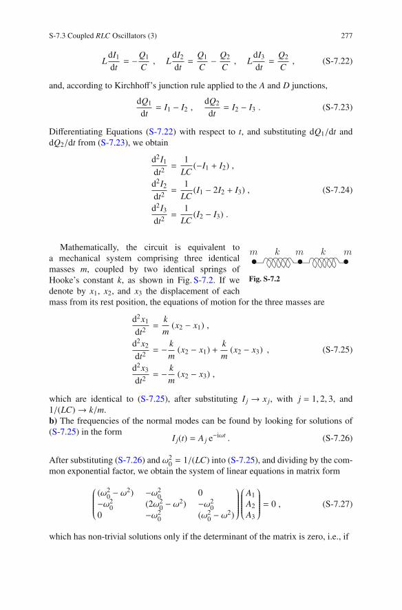
S-7.3 Coupled RLC Oscillators (3) 277
LdI1
dt= −Q1
C, L
dI2
dt=
Q1
C− Q2
C, L
dI3
dt=
Q2
C, (S-7.22)
and, according to Kirchhoff’s junction rule applied to the A and D junctions,
dQ1
dt= I1 − I2 ,
dQ2
dt= I2 − I3 . (S-7.23)
Differentiating Equations (S-7.22) with respect to t, and substituting dQ1/dt and
dQ2/dt from (S-7.23), we obtain
d2I1
dt2=
1
LC(−I1 + I2) ,
d2I2
dt2=
1
LC(I1 − 2I2 + I3) , (S-7.24)
d2I3
dt2=
1
LC(I2 − I3) .
k mm k m
Fig. S-7.2
Mathematically, the circuit is equivalent to
a mechanical system comprising three identical
masses m, coupled by two identical springs of
Hooke’s constant k, as shown in Fig. S-7.2. If we
denote by x1, x2, and x3 the displacement of each
mass from its rest position, the equations of motion for the three masses are
d2x1
dt2=
k
m(x2 − x1) ,
d2x2
dt2= − k
m(x2 − x1) +
k
m(x2 − x3) , (S-7.25)
d2x3
dt2= − k
m(x2 − x3) ,
which are identical to (S-7.25), after substituting I j → x j, with j = 1, 2, 3, and
1/(LC)→ k/m.
b) The frequencies of the normal modes can be found by looking for solutions of
(S-7.25) in the formI j(t) = A j e−iωt . (S-7.26)
After substituting (S-7.26) and ω20= 1/(LC) into (S-7.25), and dividing by the com-
mon exponential factor, we obtain the system of linear equations in matrix form
⎛
⎜
⎜
⎜
⎜
⎜
⎜
⎜
⎜
⎝
(ω20− ω2) −ω2
00
−ω20
(2ω20− ω2) −ω2
0
0 −ω20
(ω20− ω2)
⎞
⎟
⎟
⎟
⎟
⎟
⎟
⎟
⎟
⎠
⎛
⎜
⎜
⎜
⎜
⎜
⎜
⎜
⎜
⎝
A1
A2
A3
⎞
⎟
⎟
⎟
⎟
⎟
⎟
⎟
⎟
⎠
= 0 , (S-7.27)
which has non-trivial solutions only if the determinant of the matrix is zero, i.e., if

278 S-7 Chapter Solutions for Chapter 7
(
ω20 − ω
2) [(
2ω20 − ω
2) (
ω20 − ω
2)
− ω40
]
− ω40
(
ω20 − ω
2)
= 0 . (S-7.28)
Equation (S-7.28) is a cubic equation in ω2, in the following we shall consider only
the corresponding nonnegative values of ω. A first solution is ω = ω0 = Ω1. If we
substitute ω = Ω1 into (S-7.27) we obtain A1 = −A3, and A2 = 0, corresponding to
zero current in the central mesh, and I1 and I2 oscillating with opposite phases. For
the mechanical system of Fig. S-7.2, this solution corresponds to the central mass at
rest, while the left and right masses oscillate with opposite phases.
Dividing (S-7.28) by (ω20− ω2) we obtain the equation
− 3ω20ω
2 + ω4 = 0 , (S-7.29)
which has the two solutions ω =√
3ω0 = Ω2 and ω = 0 = Ω3. The mode of zero
frequency (Ω3) corresponds to a DC current I = I1 = I2 = I3 flowing freely through
the inductors, while I1 and I2 cancel out in branch AB, and I2 and I3 cancel out in
branch DE. For the mechanical system, this solution correspond to a pure transla-
tional motions of the three masses.
Substituting Ω2 into (S-7.27) we obtain
A2 = −2A1 , A3 = A1 , (S-7.30)
i.e., I1 and I3 have the same amplitude and oscillate in phase, while I2 oscillates with
double amplitude and opposite phase. The two external masses of Fig. S-7.2 oscil-
late in phase, at constant distance from each other, while the central mass oscillates
with opposite phase and double amplitude, so that the center of mass is at rest.
The three quantities
J0 = I1 + I2 + I3 , J1 = I1 − I3 , J2 = I1 − 2I2 + I3 , (S-7.31)
corresponding to the three normal modes of the circuits, oscillate at the frequencies
Ω0 = 0, Ω1, and Ω2, respectively.
c) Taking the finite resistances into account, (S-7.22) become
dI1
dt+ RI1 = −
Q1
C,
dI2
dt+ RI2 =
Q1
C− Q2
C,
dI3
dt+ RI3 =
Q2
C, (S-7.32)
which give for the normal modes
d2J0
dt2+
R
L
dJ0
dt= 0 ,
d2J1
dt2+
R
L
dJ1
dt+ Ω2
1J1 = 0 , (S-7.33)
d2J2
dt2+
R
L
dJ2
dt+ Ω2
2J2 = 0 .

S-7.3 Coupled RLC Oscillators (3) 279
The solution for J0 describes a non-oscillating, exponentially decreasing current
J0 = C0 e−γt, with decay rate γ = R/L. The last two equations describe damped
oscillating currents J1,2 = C1,2 exp(−iΩ1,2t − γt), with
Ω1,2 =
√
ω21,2− γ
2
4, (S-7.34)
where we have assumed Ω1,2 > γ/2.
S-7.4 The LC Ladder Network
a) Let Qn be the charge on the nth capacitor. Kirchhoff’s junction rule at junction D
of Fig. 7.4 impliesdQn
dt= In−1 − In , (S-7.35)
while Kirchhoff’s mesh rule applied to mesh DEFG implies
Qn
C− Qn+1
C= L
dIn
dt. (S-7.36)
Now we differentiate (S-7.36) with respect to time, and insert (S-7.35) for the deriv-
atives of Qn, obtaining
d2In
dt2= ω2
0 (In−1 − 2In + In+1) , where ω20 =
1
LC. (S-7.37)
κ m
xn−1 xn xn+1
Fig. S-7.3
The equivalent mechanical system is a linear sequence of N identical masses m,
each pair of consecutive masses being bound to each other by a spring of Hooke’s
constant κ (we use the Greek letter κ here because we shall need the letter k for the
wavevector later on), as shown in Fig. S-7.3. We denote by xn the displacement of
each mass from its equilibrium position, i.e., its position when all springs have their
rest length. Thus, the equation of motion of the nth mass is
md2xn
dt2= −κ (xn − xn−1) + κ (xn+1 − xn) , (S-7.38)
which, divided by m, and after introducing ω20= κ/m becomes

280 S-7 Chapter Solutions for Chapter 7
d2xn
dt2= ω2
0 (xn−1 − 2xn + xn+1) , (S-7.39)
mathematically equivalent to (S-7.37). This equation can be generalized to the case
of a mechanical system where transverse displacements are allowed, in addition to
the longitudinal displacements. If the masses can move in three dimensions, and we
denote by rn the displacement of the nth mass from its equilibrium position, the
equation of motion is written
d2rn
dt2= ω2
0 (rn−1 − 2rn + rn+1) ,
which is separable into three one-dimensional equations, each identical to (S-7.37).
b) First, we note that, without loss of generality, we can assume the wavevector k
appearing in Equation (7.3) to be positive (k > 0), so that (7.3) represents a wave
traveling from left to right. Changing the sign of k simply gives a wave of the same
frequency propagating in the opposite direction, whose dispersion relation is the
same as for the forward-propagating wave, because of the inversion symmetry of
the problem.
Inserting (7.3) in (S-7.37), and dividing both sides by Ce−iωt we obtain
− ω2 eikna = ω20
[
eik(n+1)a − 2eikna + eik(n−1)a]
, (S-7.40)
where, again, we have substitutedω20= 1/LC. Dividing both sides by eikna we obtain
ω2 = ω20
(
2 − eika − e−ika)
= 2ω20 (1 − cos ka) = 4ω2
0 sin2(ka/2) , (S-7.41)
O
2ω0
π
a
ω
k
Fig. S-7.4
or, performing the square root,
ω = 2ω0
∣
∣
∣
∣
∣
∣
sin
(
ka
2
)∣
∣
∣
∣
∣
∣
. (S-7.42)
The dispersion relation (S-7.42) is shown in
Fig. S-7.4 for 0 < k ≤ π/a, this range being
sufficient to describe all waves propagating in
the system. In fact, although (S-7.42) seems
to imply that ω(k) is a periodic function of
k, with period 2π/a, the wavevectors k and
k′ = k + 2πs/a, with s any integer, actually represent the same wave, since
eik′na = ei(k+2πs/a)na = eiknae2πisn = eikna , (S-7.43)
sn being an integer. This is why it is sufficient to consider the range 0 < k ≤ π/a.

S-7.4 The LC Ladder Network 281
x = na
x = na
t = t1I
I
t = t1 +π
ω
O
O
(n − 1) a
na
na
(n + 1) a(n − 1) a
(n + 1) a
Fig. S-7.5
The existence of a maximum
wave vector and of a cut-off fre-
quency is related to the discrete
periodic nature of the network,
which imposes a minimum sam-
pling rate a. The value kmax = π/a
corresponds to λmin = 2π/kmax =
2a, and waves with a smaller
wavelength cannot exist. In these
waves, the current intensity value
is repeated every two meshes
of the network, as shown in
Fig. S-7.5. A wave with a smaller
period cannot exist because of the geometry of the network. One can also note that
the direction of wave propagation cannot be determined by observing the wave pro-
file a two instants t1 and t1 + π/ω (half a period later, upper and lower parts of
Fig. S-7.5). This is consistent with the group velocity vg(kmax) = (∂kω)(kmax) = 0.
The maximum wavevector corresponds to a high cut-off frequency ωmax = 2ω0.
Since higher frequencies cannot be transmitted, the LC network is a low-pass fil-
ter.
c) The general monochromatic solution of frequency ω is a standing wave, i.e., the
sum of two waves, one propagating from left to right and the other form right to left
In(t) = Aeikna−iωt + Be−ikna−iωt , (S-7.44)
where ω and k are related by the dispersion relation (S-7.42). Because of our bound-
ary conditions we must have
x0(t) = 0⇒ A + B = 0 ; xN(t) = 0⇒ AeikNa + Be−ikNa = 0. (S-7.45)
This gives the condition eikNa − e−ikNa = 2i sin(kNa) = 0, i.e., k = πl/Na with l =
1, 2, 3, . . . ,N − 1,N. We have N allowed wavevectors kl and frequencies ωl = ω(kl).
Note that kmin = π/Na corresponds to λmax = 2π/kmin = 2Na, this is a standing
wave of wavelength twice the length of the system.
d) We obtain the limit to a continuous by letting a→ 0 and n→ ∞ with na = x =
constant so that
lima→0
In+1(t) − 2In(t) + In−1(t)
a2= lim
a→0
I(x + a, t) − 2I(x, t) + I(x − a, t)
a2
= ∂2xI(x, t) . (S-7.46)
At this limit we can define a capacity per unit length Cℓ, and an inductance per
unit length Lℓ, of the circuit, such that the capacitance and inductance of a circuit
segment of length ∆x are, respectively,

282 S-7 Chapter Solutions for Chapter 7
C = Cℓ∆x and L = Lℓ∆x. (S-7.47)
If we further introduce the quantity
v =
√
1
LℓCℓ, (S-7.48)
which has the dimensions of a velocity, (S-7.37) is written for the continuous system
∂2t I(x, t) = lim
a→0
v2
a2[I(x + a, t) − 2I(x, t) + I(x − a, t)]
= v2 ∂2
xI(x, t) . (S-7.49)
This is the equation for a wave propagating with velocity v, independent of the
wave frequency ω. At the limit of a continuous system there is no dispersion. This
is the case of ideal transmission lines, like parallel wires and coaxial cables with no
resistance. See Prob. 7.6 for the case of a realistic transmission line with resistive
losses where, however, dispersion can be eliminated.
S-7.5 The CL Ladder Network
a) We have the same electric potential on the lower horizontal branch of each mesh,
and we assume it to be zero. The voltage drop across the nth capacitor is
Vn−1 − Vn =Qn
C. (S-7.50)
The current in the nth inductor is In − In+1, corresponding to a voltage drop across
the inductor L (dIn/dt − dIn+1/dt). Thus we have
Vn−1 = L
(
dIn−1
dt− dIn
dt
)
, Vn = L
(
dIn
dt− dIn+1
dt
)
, (S-7.51)
which, inserted into (S-7.50), give
L
(
dIn−1
dt− 2
dIn
dt+
dIn+1
dt
)
=Qn
C. (S-7.52)
Differentiating (S-7.52) with respect to time, and using dQn/dt = In, we obtain
L
(
d2In−1
dt2− 2
d2In
dt2+
d2In+1
dt2
)
=In
C, (S-7.53)
which is (7.4).

S-7.5 The CL Ladder Network 283
b) By substituting In = Aeikna−iωt and In±1 = Aeik(n±1)a−iωt into (S-7.53), defining
ω20= (LC)−1, and dividing both sides by LA eikna−iωt, we obtain
− ω2(
eika − 2 + e−ika)
= ω20 . (S-7.54)
The left-hand side can be rewritten
−ω2(
eika − 2 + e−ika)
= −ω2 [2 cos(ka) − 2] = −2ω2 [cos(ka) − 1]
= −2ω2
[
cos(ka) − cos2
(
ka
2
)
− sin2
(
ka
2
)]
= −2ω2
[
cos2
(
ka
2
)
− sin2
(
ka
2
)
− cos2
(
ka
2
)
− sin2
(
ka
2
)]
= 4ω2 sin2
(
ka
2
)
. (S-7.55)
ω
π
a
kO
ω0
2
Fig. S-7.6
Substituting into (S-7.54) we have
ω2 =ω2
0
4 sin2(ka/2), (S-7.56)
or
ω =ω0
2| sin(ka/2)|. (S-7.57)
Fig. S-7.6 shows the plot of the disper-
sion relation. Compare this behavior
with the dispersion relation shown in
Fig. S-7.4 for an LC network, where
capacitors and inductors are swapped
with respect to the present case (Problem 7.4). In the LC network 2ω0 is an upper
cut-off frequency. Here, in the CL network, we have a lower cut-off frequency ω0/2,
and the CL ladder network acts as a low-pass filter.
S-7.6 A non-dispersive transmission line
a) The voltage drop from x to x + dx is
V(x, t) − V(x + dx, t) = ∂tI(x, t)L + I(x, t)R , (S-7.58)
which yields, after replacing R by Rℓdx and L by Lℓdx,
∂xV = −Lℓ∂tI − RℓI . (S-7.59)
The charge associated to the capacitance per unit length is Q = Q(x, t) = CV(x, t),
and charge conservation yields

284 S-7 Chapter Solutions for Chapter 7
∂tQ(x, t) = I(x − dx, t) − I(x, t) − IL(x, t) , (S-7.60)
with the leakage current given by
IL = IL(x, t) = V(x, t)/Rp = V(x, t) Gℓdx . (S-7.61)
We thus obtain, by eliminating Q and replacing C by Cℓdx,
Cℓ∂tV = −∂xI −GℓV . (S-7.62)
Now we eliminate V by calculating
∂2xI = −Cℓ∂t∂xV −Gℓ∂xV
= +LℓCℓ∂2t I +CℓRℓ∂tI +GℓLℓ∂tI +GℓRℓI , (S-7.63)
which yields Eq. (7.6).
b) By substituting (7.7) in (7.6) we obtain
− k2 +ω2
v20
= −iω(RℓCℓ + LℓGℓ) + RℓGℓ , (S-7.64)
where v20= (LℓCℓ)
−1. Thus, the wavevector k is a complex number. Writing k =
kr + iki we obtain
k2r − k2
i =ω2
v20
− RℓGℓ , (S-7.65)
2krki = ω(RℓCℓ + LℓGℓ) . (S-7.66)
The wave is thus evanescent,
I(x, t) = I0e−ki xeikr x−iωt , (S-7.67)
where the acceptable values for ki are positive. Since in general kr = kr(ω) if Rℓ 0
or Gℓ 0, resistive effects make the line to be dispersive, so that a wavepacket is
distorted along its propagation.
c) If we assume that k2i= RℓGℓ in (S-7.65), then kr = ω/v0, which means that the
propagation is non-dispersive: the phase velocity vp = ω/kr = v0 is independent of
frequency. In addition, since ki does not depend on ω, the evanescence length k−1i
is also frequency-independent. By substituting ki =√
RℓGℓ and kr = ω(LℓCℓ)1/2 in
(S-7.66) we obtain the condition
2√
RℓGℓ√
LℓCℓ = RℓCℓ + LℓGℓ . (S-7.68)
Squaring both sides and rearranging the terms yields (RℓCℓ − LℓGℓ)2 = 0, which
leads to the simple, equivalent condition

S-7.6 A non-dispersive transmission line 285
RℓCℓ = LℓGℓ . (S-7.69)
This is the condition for a non-dispersive or distortionless transmission line due to
O. Heaviside.
If the input current at one side of the line, say at x = 0, is
I(0, t) = I0(t) =
∫
I0(ω) e−iωtdω , (S-7.70)
where I0(ω) is the Fourier transform, then the current along the line will be given
by
I(x, t) =
∫
I0(ω)eikr x−iωte−ki xdω = e−ki x
∫
I0(ω)e−iω(t−x/v0)dω
= e−ki xI0(t − x/v0) , (S-7.71)
since ki is independent on ω. This is equivalent to state that the general solution of
(7.6) with the condition (S-7.69) has the form (7.8) with v = v0 and κ = ki.
The same conclusion may be obtained by direct substitution of (7.8) into Eq. (7.6).
The partial derivatives are given by
∂tI = −ve−κx f ′(x − vt) ,
∂2t I = v
2e−κx f ′′(x − vt) ,
∂xI = −κe−κx f (x − vt) + e−κx f ′(x − vt) ,
∂2xI = κ2e−κx f (x − vt) − 2κe−κx f ′(x − vt) + e−κx f ′′(x − vt) , (S-7.72)
where f ′(x) = d f (x)/dx and f ′′(x) = d2 f (x)/dx2. Thus Eq. (7.6) becomes
(κ2 − RℓGℓ) f + (v(RℓCℓ + LℓGℓ) − 2κ) f ′ + (1 − LℓCℓv2) f ′′ = 0 . (S-7.73)
For this equation to be true for arbitrary f , the coefficients of f , f ′ and f ′′ must be
all zero. Thus
κ2 = RℓGℓ , 2κ = v(RℓCℓ + LℓGℓ) , v2 = (LℓCℓ)
−1 , (S-7.74)
which bring again the conditions on the line parameters found above.
S-7.7 An “Alternate” LC Ladder Network
a) Let Qn be the charge of the capacitor at the right of mesh n. Applying Kirchhoff’s
mesh rule to the even and odd meshes of the ladder network we have, respectively,
− Q2n−1
C+ L2
dI2n
dt+
Q2n
C= 0 , −Q2n
C+ L1
dI2n+1
dt+
Q2n+1
C= 0 , (S-7.75)
while Kirchhoff’s junction rule gives

286 S-7 Chapter Solutions for Chapter 7
dQ2n−1
dt= I2n−1 − I2n ,
dQ2n
dt= I2n − I2n+1 . (S-7.76)
Differentiating (S-7.75) with respect to time, and inserting (S-7.76), we obtain
L2d2I2n
dt2=
1
C
(
dQ2n−1
dt− d2Q2n
dt2
)
=1
C(I2n−1 − 2I2n + I2n+1)
L1d2I2n+1
dt2=
1
C
(
dQ2n
dt− d2Q2n+1
dt2
)
=1
C(I2n − 2I2n+1 + I2n+2) , (S-7.77)
identical to (7.9).
M Mm mκ κ κ κκ
x2n−1 x2n x2n+1 x2n+2
Fig. S-7.7
A mechanical equivalent to our network is the one-dimensional sequence of
masses and springs shown in Fig. S-7.7, where the masses have, alternately, the val-
ues M and m, while all springs are identical, with Hooke’s constant κ. If we denote
by x2n+1 the positions of the odd masses M, and by and x2n the positions of even
masses m, the equations of motion for the system are
md2x2n
dt2= −κ(x2n − x2n+1) + κ(x2n−1 − x2n) = κ(x2n−1 − 2x2n + x2n+1)
Md2x2n+1
dt2= −κ(x2n+1 − x2n+2) + κ(x2n − x2n+1) = κ(x2n − 2x2n+1 + x2n+2),
(S-7.78)
which, after the substitutions m→ L2, M → L1, x→ I, and κ → 1/C, are identical
to (S-7.77).
b) Substituting (7.10) into (S-7.77), and dividing both sides by e−iωt, we obtain
−ω2L2Ie ei(2n) ka =1
C
(
Io ei(2n−1) ka − 2Ie ei(2n) ka + Io ei(2n+1) ka)
−ω2L2Io ei(2n+1) ka =1
C
(
Ie ei(2n) ka − 2Io ei(2n+1) ka + Ie ei(2n+2) ka)
. (S-7.79)
Now we define the two angular frequencies ωo = 1/√
L1C and ωe = 1/√
L2C, and
divide (S-7.79) by ei(2n) ka, obtaining
(2ω2e − ω2) Ie − 2ω2
e cos(ka) Io = 0
2ω2o cos(ka) Ie − (2ω2
o − ω2) Io = 0 . (S-7.80)

S-7.7 An “Alternate” LC Ladder Network 287
This system of linear equations has non-trivial solutions if and only if its determi-
nant is zero, i.e., if
(2ω2e − ω2)(2ω2
o − ω2) − 4ω2oω
2e cos2(ka) = 0 , (S-7.81)
the solution of this quadratic equation in ω2 is
ω2 = ω2e + ω
2o ±
√
(
ω2e + ω
2o
)2− 4ω2
oω2e sin2(ka) . (S-7.82)
Both solutions are physically acceptable: the system allows for two types of propa-
gating waves, described by two different dispersion relations.
At the limit L2 ≪ L1 (or m ≪ M, for the equivalent mechanical system) we have
ω2o ≪ ω2
e , and (S-7.82) can be approximated as
ω2 ≃ ω2e + ω
2o ± ω2
e
√
1 + 2ω2
o
ω2e
− 4ω2
o
ω2e
sin2(ka) (S-7.83)
where we have disregarded the fourth-order term ω4o/ω
4e inside the square root.
If we further use the approximation√
1 + x ≃ 1 + x/2, valid for x ≪ 1, (S-7.83)
becomes
ω2 ≃ ω2e + ω
2o ± ω2
e
1 +ω2
o
ω2e
[
1 − 2 sin2(ka)]
, (S-7.84)
corresponding to the two dispersion relations
ω ≃⎧
⎪
⎪
⎨
⎪
⎪
⎩
√
2(ω2e + ω
2o) − 2ω2
o sin2(ka)√2ωo sin(ka)
(S-7.85)
κOπ
a
ω1
ω2
ω
ω3
Fig. S-7.8
The lower branch can propagate for fre-
quencies between 0 and ω1 =√
2ωo, while
the upper branch lies between ω2 =
ωe
√
2(1 − ω2o/ω
2e) and ω3 =
√2ωe. Thus,
there is a gap of “forbidden” frequencies
between ω1 and ω2. Figure S-7.8 shows the
exact solution (continuous lines), and the
approximate solution (dashed lines), still in
good agreement, for ω2o/ω
2e = 0.25.
Of course, the two branches are present
also in the case of the alternating mechanical
oscillators, and provide a model for an effect
known in solid state physics. The vibrations

288 S-7 Chapter Solutions for Chapter 7
of a lattice formed by identical ions have a single branch (Problem 7.4), with a dis-
persion relation similar to the lower branch, which is named “acoustic branch”. In
an ionic crystal, formed by two ion species alternating on the sites of the lattice, we
observe also the upper branch, named “optical branch”.
S-7.8 Resonances in an LC Ladder Network
a) According to Problem 7.4, the current flowing in the nth mesh is
d2In
dt2= ω2
0(In+1 − 2In + In−1) . (S-7.86)
We are looking for a propagating wave solution, and define the phase
φ ≡ ka , (S-7.87)
where a is the length of a single mesh, to be substituted into (S-7.44), writing In(t)
as
In(t) = Aeinφ−iωt . (S-7.88)
Substituting (S-7.88) into (S-7.86), and dividing by e−iωt, we get
− ω2einφ = ω20
[
ei(n+1)φ − 2einφ + ei(n−1)φ]
, (S-7.89)
from which we obtain the dispersion relation
ω2 = ω20 (2 − eiφ − e−iφ) = 2ω2
0 (1 − cos φ) = 4ω20 sin2(φ/2) , (S-7.90)
whose inverse is
sin
(
φ
2
)
=ω
2ω0, or φ = 2 arcsin
(
ω
2ω0
)
, (S-7.91)
that shows that φ is a real number if ω < 2ω0.
Due to the presence of the current source, (S-7.88) holds if the current in the 0th
mesh is
I0(t) = Ise−iωt , (S-7.92)
thus we must have A = Is, and the final expression for In(t) is
In(t) = Iseinφ−iωt , (S-7.93)
where φ is given by (S-7.91)

S-7.8 Resonances in an LC Ladder Network 289
b) Ifω > 2ω0 the current wave cannot propagate in the ladder. We look for a solution
of the form suggested by the hint. Substituting (7.12) into (S-7.86) we obtain
− ω2α−n = ω20
[
α−(n+1) − 2α−n + α−(n−1)]
, (S-7.94)
which, multiplied by αn/ω20, turns into
α2 +
⎛
⎜
⎜
⎜
⎜
⎜
⎝
ω2
ω20
− 2
⎞
⎟
⎟
⎟
⎟
⎟
⎠
α + 1 = 0 . (S-7.95)
The solutions are
α = 1 − ω2
2ω20
±
√
√
⎛
⎜
⎜
⎜
⎜
⎜
⎝
1 − ω2
2ω20
⎞
⎟
⎟
⎟
⎟
⎟
⎠
2
− 1 . (S-7.96)
We must have |α| < 1 for an infinite ladder, otherwise the current would grow indef-
initely in successive meshes. Thus, we keep the solution with the plus sign, because
ω > 2ω0 implies that all solutions of (S-7.96) are negative, obtaining
In(t) = Is(−1)n|α|ne−iωt, |α| = ω2
2ω20
− 1 −
√
√
⎛
⎜
⎜
⎜
⎜
⎜
⎝
ω2
2ω20
− 1
⎞
⎟
⎟
⎟
⎟
⎟
⎠
2
− 1 , (S-7.97)
that we can rewrite as
In(t) = Is e−γn−iωt , where γ = iπ + ln |α| . (S-7.98)
c) We consider the case of the propagating wave (ω < 2ω0) first. If the ladder com-
prises N meshes numbered as in Fig. 7.8, the boundary condition at the right end is
IN(t) ≡ 0 (mesh number N does not exist!). The most general solution is the sum of
two counterpropagating waves
In(t) = Aeinφ−iωt + Be−inφ−iωt . (S-7.99)
Imposing the conditions I0 = Is and IN = 0, we obtain
A + B = Is, AeiNφ + Be−iNφ = 0 , (S-7.100)
with solutions
A = +i
2Is
e−iNφ
sin(Nφ), B = − i
2Is
e+iNφ
sin(Nφ), (S-7.101)
where φ = φ(ω) depends on ω according to (S-7.91). We observe resonances when
sin(Nφ) = 0, i.e., for φ = mπ/N with m an integer. Remembering (S-7.87)

290 S-7 Chapter Solutions for Chapter 7
N = mπ
φ= m
π
ka= mπ
a
λ
2π= m
1
a
λ
2, (S-7.102)
and, multiplying both sides by a
L = Na = mλ
2, (S-7.103)
where L is the total length of the ladder network. This corresponds to the case when
the frequency of the current source equals the frequency of one of the standing
waves allowed in the network, i.e., when the length of the ladder network is an
integer multiple of a half wavelength.
If ω > 2ω0, the general solution is
In(t) = Aαn+e−iωt + Bαn
−e−iωt, (S-7.104)
where α± = α±(ω) are the two solutions of (S-7.96). Here also the case |α| > 1 is
allowed, because |α|n cannot diverge if n is limited. The boundary conditions are
A + B = Is , AαN+ + Bα+N
− = 0 , (S-7.105)
with solutions
A = +Is
αN−
αN− − αN
+
, B = −Is
αN+
αN− − αN
+
. (S-7.106)
The A and B coefficients diverge if α− = α+ = 1, i.e., if ω = 2ω0. Thus, for ω > 2ω0
there are no resonances, but the response of the system diverges as the frequency
approaches the cut-off value, i.e. as ω→ 2ω0.
S-7.9 Cyclotron Resonances (1)
a) The rotating electric field can be written as
E = E(t) = E0 (x cosωt ± y sinωt) , (S-7.107)
where the positive (negative) sign indicates counterclockwise (clockwise) rotation.
From the equation of motion
mdv
dt= q
(
E +v
c× B
)
, (S-7.108)
we see that dvz/dt = 0, thus, if we assume that vz(0) = 0, the motion occurs in the
(x, y) plane. The equations of motion along the x and y axes are

S-7.9 Cyclotron Resonances (1) 291
dvx
dt= +qvy
B0
mc+
qE0
mcosωt
dvy
dt= −qvx
B0
mc± qE0
msinωt . (S-7.109)
In principle, we can differentiate both equations with respect to time, and then sub-
stitute the expressions for dvx,y/dt, thus obtaining two uncoupled second-order dif-
ferential equations for a driven harmonic oscillator.
But we prefer a a more “elegant” approach, introducing the complex variable
ζ = vx + ivy. The velocity is thus represented by a complex vector in the (Reζ, Imζ)
plane. Adding the second of (S-7.109), multiplied by i, to the first, we obtain
dζ
dt= −iωc ζ +
qE0
me±iωt, (S-7.110)
where ωc = qB0/mc is the cyclotron (or Larmor) frequency. The solution of the
associated homogeneous equation is
ζ(t) = A e−iωct , (S-7.111)
where A is an arbitrary complex constant. Equation (S-7.111) describes the motion
in the absence of the electric field, when the velocity rotates clockwise with fre-
quency ωc in the ζ plane. We then search for a particular integral of the inhomoge-
neous equation in the form
ζ = ζ0 e±iωt ,
and find, by direct substitution,
ζ0 = −iqE0
m (ωc ± ω). (S-7.112)
Thus the general solution of (S-7.110) is
ζ(t) = A e−iωct − iqE0
m (ωc ± ω)e±iωt . (S-7.113)
Assuming ωc > 0, we observe a resonance at ω = ωc only if the field rotates clock-
wise. In this case the electric field accelerates the particle along the direction of its
“natural” motion.
b) At resonance (ω = ωc), we search for a non-periodic solution of the form
ζ(t) = ζR(t) e−iωt , (S-7.114)
which, substituted into (S-7.110), gives

292 S-7 Chapter Solutions for Chapter 7
(
dζR
dt
)
e−iωt − iωζR e−iωt = −iωc ζR e−iωt +qE0
me−iωt , (S-7.115)
and, since ωc = ω,
(
dζR
dt
)
=qE0
m. (S-7.116)
The solution of (S-7.116) is
ζR(t) = ζ(0) +qE0
mt , (S-7.117)
which gives
ζ(t) =
[
ζ(0) +qE0
mt
]
e−iωt . (S-7.118)
The trajectory is a spiral, with the radial velocity increasing linearly with time.
c) Introducing a viscous force fv = −mγv we obtain the following equation for ζ
dζ
dt= −iωc ζ − γζ +
qE0
me−iωt . (S-7.119)
The solution has the form of (S-7.113) with ωc replaced by (ωc − iγ),
ζ = −iqE0
m(ωc − ω − iγ)e−iωt + A e−iωct−γt , (S-7.120)
where the second term undergoes an exponential decay, and any memory of the
initial conditions is lost after a transient phase, while the periodic part of the solution
does not diverge at resonance, due to the presence of iγ in the denominator. Thus,
the steady-state solution at resonance is
ζR =qE0
mγe−iωt . (S-7.121)
The average dissipated power is the time average of the instantaneous dissipated
power over a period
P = 〈f · v〉 = 〈qE · v〉. (S-7.122)
The components of the particle velocity in the steady state are
vx = Re(ζ) =qE0γ
m[
(ωc − ω)2 + γ2] cosωt − qE0 (ωc − ω)
m[
(ωc − ω)2 + γ2] sinωt ,
vy = Im(ζ) = − qE0γ
m[
(ωc − ω)2 + γ2] sinωt − qE0 (ωc − ω)
m[
(ωc − ω)2 + γ2] cosωt . (S-7.123)

S-7.9 Cyclotron Resonances (1) 293
Thus, inserting (S-7.123) and the relations
Ex = E0 cosωt , Ey = −E0 sinωt , 〈cos2 ωt〉 = 〈sin2 ωt〉 = 1
2,
〈cosωt sinωt〉 = 0 , (S-7.124)
into (S-7.122), we obtain for the average dissipated power
P =q2E2
0γ
m[
(ωc − ω)2 + γ2] . (S-7.125)
At resonance we have
P =q2E2
0
mγ. (S-7.126)
S-7.10 Cyclotron Resonances (2)
a) The equations of motion are
dvx
dt= +ωcvy +
qE0
mcosωt ,
dvy
dt= −ωcvx , (S-7.127)
where ωc = qB0/m. By differentiating (S-7.127) with respect to time, and substitut-
ing the values for vx and vy from (S-7.127) itself, we obtain the two equations
d2vx
dt2= +ωc
dvy
dt− qE0ω
msinωt = −ω2
cvx −qE0ω
msinωt ,
d2vy
dt2= −ωc
dvx
dt= −ω2
cvy −qE0ωc
mcosωt , (S-7.128)
each of which describes the velocity of a driven harmonic oscillator. The steady
state solutions are
vx =qE0ω
m (ω2 − ω2c)
sinωt , vy =qE0ωc
m (ω2 − ω2c)
cosωt . (S-7.129)
We observe a resonance if ω = |ωc|, independently on the signs of q and B0. With
respect to Problem 7.9, where a rotating electric field was assumed, here a resonance
is always found because the linearly oscillating electric field can be decomposed
into two counter-rotating fields of the same amplitude, of which one will excite the
resonance.
b) In the presence of a frictional force f = −mγv the equations of motion become

294 S-7 Chapter Solutions for Chapter 7
dvx
dt= +ωcvy − γvx +
qE0
mcosωt ,
dvy
dt= −ωcvx − γvy , (S-7.130)
and cannot be uncoupled by the procedure of point a). Analogously to Problem 7.9,
we introduce the complex quantity ζ = vx + ivy, obtaining the single equation
dζ
dt= −iωcζ − γζ +
qE0
2m
(
eiωt + e−iωt)
, (S-7.131)
where we have used Euler’s formula for the cosine. Differently from Problem 7.9,
now we search for a steady-state solution of the form
ζ = Ae−iωt + Beiωt , (S-7.132)
where A and B are two complex constants to be determined. By direct substitutioninto (S-7.131) we have
−iωAe−iωt + iωBeiωt = −(iωc + γ)Ae−iωt − (iωc + γ)Beiωt +qE0
2m
(
eiωt + e−iωt)
,
which is separable into two equations relative, respectively, to the terms rotating
clockwise and counterclockwise in the complex plane
− iωA = −(iωc + γ)A +qE0
2m, iωB = −(iωc + γ)B +
qE0
2m. (S-7.133)
The solutions for A and B are
A =qE0
2m[i(ωc − ω) + γ]=
qE0γ
2m[(ωc − ω)2 + γ2]− i
qE0(ωc − ω)
2m[(ωc − ω)2 + γ2]
B =qE0
2m[i(ωc + ω) + γ]=
qE0γ
2m[(ωc + ω)2 + γ2]− i
qE0(ωc + ω)
2m[(ωc + ω)2 + γ2],
(S-7.134)
from which we obtain the stationary-state velocity components of the particle
vx = [Re(A) + Re(B)] cosωt + [Im(A) − Im(B)] sinωt
vy = [Im(A) + Im(B)] cosωt − [Re(A) − Re(B)] sinωt . (S-7.135)
The average absorbed power is
P = 〈qv · E〉 = 〈qvxEx〉 = q[Re(A) + Re(B)]E01
2
=q2E2
0γ
4m[(ωc − ω)2 + γ2]+
q2E20γ
4m[(ωc + ω)2 + γ2], (S-7.136)

S-7.10 Cyclotron Resonances (2) 295
since Ex = E0 cosωt, 〈cos2 ωt〉 = 1/2, and 〈cosωt sinωt〉 = 0. Thus, again, we
observe a resonance at ω = |ωc|, independently of the signs of q and B0. Assum-
ing γ ≪ ωc the power absorbed at resonance is
Pmax ≃q2E2
0
4mγ. (S-7.137)
S-7.11 A Quasi-Gaussian Wave Packet
We need to evaluate the inverse transform
f (x) = A
∫ +∞
−∞e−L2(k−k0)2
eiφ(k)eikxdk
≃∫ +∞
−∞exp
[
−L2(k − k0)2 + iφ0 + iφ′0(k − k0)+
+i
2φ′′0 (k − k0)2 + i(k − k0)x + ik0x
]
dk , (S-7.138)
where, for brevity, we wrote x instead of (x − vt), and φ0, φ′0, . . . instead of φ(k0),
φ′(k0), . . . By using (7.1) we obtain
f (x) ≃ Aeik0 x+iφ0
∫ +∞
−∞exp
[
−L2(k − k0)2
(
1 − iφ′′
0
2L2
)
+ i(k − k0)(x + φ′0)
]
dk
= C exp
⎡
⎢
⎢
⎢
⎢
⎢
⎣
−(x + φ′
0)2
4L2(1 − iφ′′0/2L2)
⎤
⎥
⎥
⎥
⎥
⎥
⎦
, (S-7.139)
where C is a constant, whose value is not relevant for our purposes. By substituting
1
1 − iφ′′0
(2L2)=
1 + iφ′′0/(2L2)
1 + φ′′20/(4L4)
(S-7.140)
we obtain the wave packet profile as
f (x − vt) = C exp
⎧
⎪
⎪
⎨
⎪
⎪
⎩
−(x − vt + φ′
0)2[1 + iφ′′
0/(2L2)]
L2[1 + φ′′0
2/(4L4)]
⎫
⎪
⎪
⎬
⎪
⎪
⎭
. (S-7.141)
We thus see that the packet is wider than the purely Gaussian case, since L2[1 +
φ′′0
2/(4L4)] > L2. In addition, the center of the packet is shifted from (x − vt) to
(x − vt + φ′0), and there is an aperiodic (anharmonic) modulation due to the factor
(iφ′′0/2L2) in the numerator of the exponent.

296 S-7 Chapter Solutions for Chapter 7
S-7.12 A Wave Packet Traveling along a Weakly Dispersive Line
a) There is no dispersion if b = 0. In these conditions the signal propagates at veloc-
ity v keeping its shape:
f (x − vt) = Ae−iω0(t−x/v)e−(t−x/v)2/τ2 . (S-7.142)
b) The phase velocity and the group velocity are, by definition,
vφ =ω
k= v(1 + bk) , vg =
∂ω
∂k= v(1 + 2bk) . (S-7.143)
We can write vφ and vg as functions of ω by first inverting (7.17), obtaining for
k = k(ω)
k =
√
1
(2b)2+ω
bv
− 1
2b. (S-7.144)
Then we expand the square root to the second order in ω/v, obtaining
k ≃ ωv
− ω2b
v2. (S-7.145)
The same result can also be obtained by an iterative procedure, by inserting the first
order value for k, i.e., k = ω/v, into the bracket at the right hand side of (7.17). Thus,
the phase and group velocities to the first order are, using (S-7.143),
vφ0 ≃ v + bω0 , vg0 ≃ v + 2bω0 . (S-7.146)
c) The peak of the signal propagates at the group velocity, thus tx = x/vg0. The
spectral width of the wave packet may be estimated as ∆ω ≃ 1/τ, which corresponds
to a spread in the propagation velocity of its Fourier components
∆v ≃ v
(
2b
v
∆ω
)
≃ 2b
τ. (S-7.147)
Thus the spread of the wave packet in time and space can be estimated as
∆t ≃ ∂tx
∂vg
∆v = tx
∆v
vg
, ∆x ≃ vg∆t =2bx
vgτ. (S-7.148)
d) We approximate
k(ω) ≃ k0 + k′0(ω − ω0) +1
2k′′0 (ω − ω0)2 , (S-7.149)

S-7.12 A Wave Packet Traveling along a Weakly Dispersive Line 297
where
k′0 =∂k
∂ω
∣
∣
∣
∣
∣
ω0
≃ 1
v
− 2ω0b
v2≃ 1
vg
, k′′0 =∂2k
∂ω2
∣
∣
∣
∣
∣
∣
ω0
≃ −2b
v2. (S-7.150)
The spectrum of the wave packet (i.e., its Fourier transform) is
f (ω) =√πτAe−[ω−ω0]2τ2/4 . (S-7.151)
Since we are only interested in the behavior of the function, we evaluate the follow-
ing integral forgetting proportionality constants,
f (x, t) ∼∫
exp
[
ik(ω)x − iωt −(ω − ω0)2 τ2
4
]
dω
∼∫
exp
[
ik0x + ik′0x(ω − ω0) + ik′′
0x
2(ω − ω0)2 − (ω − ω0)2τ2
4
]
dω
∼ exp(ik0x − iω0t)
∫
exp
[
−i(t − k′0x)ω′ +
(
−τ2
4+ i
k′′0
x
2
)
ω′2]
dω′
∼ exp
⎡
⎢
⎢
⎢
⎢
⎢
⎣
ik0x − iω0t −(t − k′
0x)2
τ2 − 2ik′′0
x
⎤
⎥
⎥
⎥
⎥
⎥
⎦
. (S-7.152)
The factor which describes the envelope of the wave packet (recalling that k′0=
1/vg0) is
exp
⎡
⎢
⎢
⎢
⎢
⎣
−(t − x/vg)2
τ2 − 2ik′′0
x
⎤
⎥
⎥
⎥
⎥
⎦
= exp
⎡
⎢
⎢
⎢
⎢
⎢
⎣
−(t − x/vg)2τ2 + 2ik′′
0x
τ4 + (2k′′0
x)2
⎤
⎥
⎥
⎥
⎥
⎥
⎦
= exp
⎧
⎪
⎪
⎨
⎪
⎪
⎩
−(t − x/vg)21 + 2ik′′
0x/τ2
τ2[1 + (2k′′0
x/τ)2]
⎫
⎪
⎪
⎬
⎪
⎪
⎭
. (S-7.153)
The temporal width of the wave packet increases during the propagation as
∆t(x) = τ
√
1 +
(
2k′′0
x
τ
)2
. (S-7.154)

Chapter S-8
Solutions for Chapter 8
S-8.1 Poynting Vector(s) in an Ohmic Wire
For symmetry reasons, the magnetic field is azimuthal and depends only on the
radial coordinate r. Applying Ampere’s law to a circular path of radius r < a around
the wire axis yields2πrB =
4π
c(πr2J) , (S-8.1)
which leads toB =
2π
crσEφ , (S-8.2)
where φ is the azimuthal unit vector. Thus, the Poynting vector at a distance r from
the axis is
S =c
4πE×B = −r
σ
2E2 . (S-8.3)
a
rJ
dAS
S
dA
h
Fig. S-8.1
The energy flux ΦS ≡ Φ(S) through the sur-
face of a cylinder of radius r < a and length h
and coaxial to the wire is thus
ΦS =
∮
S ·dA = −2πrhS (r)
= −πr2hσE2 , (S-8.4)
where dA is the vector surface element of the
cylinder. The energy flows inwards, and is entirely dissipated into Joule heating
inside the cylinder volume, as we can check by calculating
W =
∫
J ·EdV = πr2hJE = πr2hσE2 , (S-8.5)
c© Springer International Publishing AG 2017
A. Macchi et al., Problems in Classical Electromagnetism,
DOI 10.1007/978-3-319-63133-2 21
299

300 Chapter S-8 Solutions for Chapter 8
where the integral is extended to the volume the cylinder. The equality W = −ΦS
satisfies Poynting’s theorem since there is no variation in time of the EM energy.
Note that, in the approximation of an infinitely long wire, the electric field is
uniform also for r > a (in the case of a finite wire of length 2h≫ a, this is a good
approximation in the central region for r≪ h, see Problem 4.9), while the magnetic
field B = 2πJa2/rc. Within this approximation, S = −(a2σE2/2r)r for r > a, so that
the energy flux is independent of r and it is still equal to minus the total dissipated
power:ΦS = −2πrhS (r) = −πa2hσE2 (r > a) . (S-8.6)
b) We must show that ∇ · (S−S′) = 0, i.e., that S−S′ = ∇× f, where f is a vector
function of the coordinates. Let us substitute E = −∇ϕ into (8.7)
S =c
4πE×B = −
c
4π∇ϕ×B . (S-8.7)
Now from the vector identity
∇× (ϕB) = ∇ϕ×B+ϕ∇×B = ∇ϕ×B+ϕ
(
4π
cJ
)
(S-8.8)
we obtain
∇ϕ×B = ∇× (ϕB)−ϕ
(
4π
cJ
)
, (S-8.9)
which can be substituted into (S-8.7), leading to
S = ϕJ−c
4π∇× (ϕB) . (S-8.10)
Thus, we are free to redefine the Poynting vector as
S′ = ϕJ, (S-8.11)
since
S−S′ = ∇×
(
−c
4πϕB
)
. (S-8.12)
a
rJ
dAS
S
dA
h
Fig. S-8.2
We can show that S′ is equivalent to S by
computing its flux through the same cylindri-
cal surface as above. Since S′ is parallel to
the wire axis, only the two base surfaces con-
tribute to the flux ΦS ′ ≡Φ(S′)
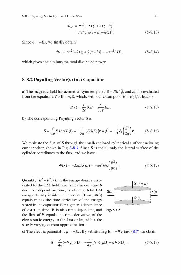
S-8.1 Poynting Vector(s) in an Ohmic Wire 301
ΦS ′ = πa2[−S (z)+S (z+h)]
= πa2J[ϕ(z+h)−ϕ(z)] . (S-8.13)
Since ϕ = −Ez, we finally obtain
ΦS ′ = πa2[−S (z)+S (z+h)] = −πa2hJE , (S-8.14)
which gives again minus the total dissipated power.
S-8.2 Poynting Vector(s) in a Capacitor
a) The magnetic field has azimuthal symmetry, i.e., B = B(r) φ, and can be evaluated
from the equation c∇×B = ∂tE, which, with our assumption E = E0 t/τ, leads to
B(r) =r
2c∂tE =
r
2cτE0 . (S-8.15)
b) The corresponding Poynting vector S is
S =c
4πE z× (B φ) = −
r
8π(E∂tE)
(
z× φ)
= −1
2∂t
(
E2
8π
)
r. (S-8.16)
We evaluate the flux of S through the smallest closed cylindrical surface enclosing
our capacitor, shown in Fig. S-8.3. Since S is radial, only the lateral surface of the
cylinder contributes to the flux, and we have
Φ(S) = −2πahS (a) = −πa2h∂t
(
E2
8π
)
. (S-8.17)
S(a
S (z + h)
S (z)
S(a)
Fig. S-8.3
Quantity (E2+B2)/8π is the energy density asso-
ciated to the EM field, and, since in our case B
does not depend on time, is also the total EM
energy density inside the capacitor. Thus, Φ(S)
equals minus the time derivative of the energy
stored in the capacitor. For a general dependence
of Ez(t) on time, B is also time-dependent, and
the flux of S equals the time derivative of the
electrostatic energy to the first order, within the
slowly varying current approximation.
c) The electric potential is ϕ = −Ez. By substituting E = −∇ϕ into (8.7) we obtain
S =c
4π(−∇ϕ)×B = −
c
4π
[
∇× (ϕB)−ϕ∇×B]
. (S-8.18)

302 Chapter S-8 Solutions for Chapter 8
Thus, the vector
S′ ≡c
4πϕ∇×B =
1
4πϕ∂tE = S+
c
4π∇× (ϕB) (S-8.19)
equals S plus the curl of a vector function, and is thus another suitable Poynting
vector. Since S′ is perpendicular to the capacitor plates, its flux through our closed
cylindrical surface is (see Fig. S-8.3)
Φ(S′) = πa2 [
S ′(z+h)−S ′(z)]
= −πa2h
(
E∂tE
4π
)
= −πa2h∂t
(
E2
8π
)
,
(S-8.20)
in agreement with (S-8.17).
S-8.3 Poynting’s Theorem in a Solenoid
a) We take a cylindrical coordinate system with the z axis along the solenoid axis.
Inside an infinite solenoid the magnetic field is uniform and equals B = B z =
(4π/c)nI z. According to Faraday’s law of induction, the rate of change of B = B(t),
due to the time dependence of I = I(t), generates an electric field E associated to the
induced electromotive force. For symmetry reasons, the field lines of E are circles
coaxial to the solenoid, i.e., we have E = E(r) φ. Applying Faraday’s law to a circle
of radius r < a, coaxial to the solenoid, we have
2πrE(r) = −πr2 1
c∂tB = −πr
2 4πnI0
c2τ, (S-8.21)
from which E(r) = −2πnI0r/(c2τ).
b) The Poynting vector inside the solenoid (r < a) is
S =c
4πE×B = −
2π (nI0)2 rt
(cτ)2(φ× z) = −
2π (nI0)2t
(cτ)2r . (S-8.22)
Thus, the flux of S = S(r) through the surface of a closed cylinder of radius r and
height h is nonzero only through the lateral surface, and we have
Φ(S) = 2πrhS · r = −
(
2πnI0r
cτ
)2
ht . (S-8.23)

S-8.3 Poynting’s Theorem in a Solenoid 303
The magnetic energy enclosed by the cylinder surface is
UM = uMV =B2
8ππr2h = 2π2r2h
(
nI0 t
cτ
)2
, (S-8.24)
where V is the volume of the cylinder, thus
dUM
dt= 4π2r2ht
(
nI0
cτ
)2
= −Φ(S) , (S-8.25)
according to Poynting’s theorem, since the electric field is constant in time, and
J ·E = 0 for r < a, i.e., inside the solenoid.
c) Outside the solenoid (r > a) we have B = 0. Correspondingly, also S = 0 and
Φ(S) = 0. The rate of change of the magnetic energy is given by (S-8.25) with r = a,
and must equal the volume integral of J ·E, which is the work done by the induced
field on the current flowing in the coils (notice that this is different from the electric
field driving the current and causing Joule heating in the coils, see Problem 13.18).
In our representation, the current is distributed on the surface r = a, thus Jd3r is
replaced by nI dS = nIadφdz in the integral, and E is evaluated at r = a. We thus
obtain
∫
V
J ·Ed3r =
∫
S
nI E(a)dS = −2πah
(
nI0t
τ
)
(
2πnI0 a
c2τ
)
= −4πa2ht
(
nI0
cτ
)2
= −dUM
dt
∣
∣
∣
∣
∣
r=R. (S-8.26)
S-8.4 Poynting Vector in a Capacitor with Moving Plates
a) We use a cylindrical coordinate system (r,φ,z), with the z axis along the symmetry
axis of the capacitor, and the origin on the fixed plate. Thus, within the limits of our
approximations, the electric field is uniform and parallel to z inside the capacitor,
whose capacitance is
C =πa2
4πh(t)=
a2
4(h0+ vt). (S-8.27)
In the case of the isolated plates the charge is constant and equal to Q0, while the
voltage between the plates V and the electric field E between the plates are, respec-
tively,
V =Q0
C= Q0
4(h0+ vt)
a2, E =
V
h=
4Q0
a2. (S-8.28)

304 Chapter S-8 Solutions for Chapter 8
In the case of constant voltage between the plates, V = V0, the charge Q of the
capacitor and the electric field E are, respectively.
Q =CV0 = V0a2
4(h0+ vt), E =
V0
h0+ vt. (S-8.29)
In the case of constant charge, the electrostatic force between the plates Fes is also
constant and equals
Fes = −QE
2= −
2Q20
a2, (S-8.30)
while in the case of constant voltage we have
Fes = −QE
2= −V2
0
a2
8(h0+ vt)2, (S-8.31)
in both cases the minus signs means that the force is attractive. In both cases the
applied external force Fmech must cancel the electrostatic force, i.e., we must have
Fmech = −Fes, for the plates to move at constant velocity.
b) The electrostatic energy can be written as
U =1
2
Q2
C=
1
2CV2 , (S-8.32)
so that at constant charge we have
U = Q20
2(h0+ vt)
a2,
dU
dt=
2vQ20
a2> 0 , (S-8.33)
while at constant voltage we have
U = V20
a2
8(h0+ vt),
dU
dt= −
a2vV20
8(h0+ vt)2< 0 . (S-8.34)
c) At constant charge, the electric field E= E0 z is also constant, with E0 =Q0/(πa2),
therefore the displacement current density JD = ∂tE/c is zero. Also the conduction
current density JC is zero between the plates (actually, there is a conduction current
localized on the moving plate, we shall come back to this point below), so that also
the magnetic field B is zero between the plates.

S-8.4 Poynting Vector in a Capacitor with Moving Plates 305
At constant voltage, the electric field is E = zV0/h(t) = zV0/(h0 + vt), implying
the presence of a displacement current along z. The magnetic field can be calculated
by taking the path integral of B over a circumference of radius r < a coaxial with,
and located between, the plates, which equals the flux of the displacement current
through the enclosed circle. Due to the cylindrical symmetry of the system, the only
nonzero component of B is azimuthal, B = B(r, t) φ, and calculating its path integral
over the circle of radius r corresponding to a field line we have for B = B(r, t)
2πrB = −πr2
c∂tE = −
πr2
c
V0 v
(h0+ vt)2, (S-8.35)
so that
B = −r
2c
V0 v
(h0+ vt)2. (S-8.36)
d) At constant charge we have B = 0, and the Poynting vector S = (c/4π)E×B is
also zero. In this case, (S-8.30) and (S-8.33) tell us that the rate of work done against
the electric force Wmech
Wmech = Fmech · v = −Fes · v =2Q2
0v
a2(S-8.37)
equals the rate of change the electrostatic energy dU/dt. This rate of work must
also equal minus the integral of J ·E over the whole space, according to Poynting’s
theorem. We verify this at the end of this answer.
At constant voltage, the Poynting vector is radial, S = S r, and, according to
(S-8.29) and (S-8.36), we have
S = −c
4πEzBφ =
V20
vr
8π (h0+ vt)3. (S-8.38)
Evaluating the flux of S through the minimum closed surface enclosing the capaci-
tor, of lateral surface 2πa (h0+ vt), we obtain
ΦS = 2πa(h0+ vt)V2
0va
8π (h0+ vt)3=
a2V20
v
4(h0+ vt)2. (S-8.39)
Through (S-8.31) and (S-8.34) we can verify that
−ΦS =dU
dt+Fv . (S-8.40)

306 Chapter S-8 Solutions for Chapter 8
Note also that, in this case, ΦS equals the power absorbed by the voltage source. In
fact, the current flowing through the circuit is
I =dQ
dt= −
a2v
4(h0+ vt)2V0 , (S-8.41)
where we have inserted the first of (S-8.29), corresponding to a power absorption
by the source
W = −V0 I =a2v
4(h0+ vt)2V2
0 =Φs . (S-8.42)
We avoided so far to discuss the role of the conduction current circulating in the
plates [the following discussion will require some familiarity with the distributions
δ(x) and Θ(x), where Θ(x) is the Heaviside step function, defined by Θ(x) = 1 for
x > 0 and Θ(x) = 0 for x < 0; notice that dΘ(x)/dx = δ(x)]. Let us consider the
constant charge case. Since the upper plate has a charge Q0 distributed on the surface
z = −h0+ vt and moves with velocity v, there is actually a current density
JC =Q0
πa2vδ(z−h0− vt) . (S-8.43)
On the other hand, the electric field between the plates may be written as
E = −4Q0
a2[Θ(z)−Θ(z−h0− vt)] z , (S-8.44)
where Θ(z) is the Heaviside step function, defined by Θ(z) = 1 for z > 0 and Θ(z) = 0
for z < 0. This expression takes into account the fact that at each time t the field
exists only in the 0 < z < vt region, so it is actually a time-dependent field. Since
dΘ(z)/dz = δ(z), the displacement current is
JD =1
c∂tE = −
4Q0v
a2cδ(z−h0− vt) z = −
4π
cJC , (S-8.45)
so that the source term for the magnetic field (4π/c)JC +JD is zero. It also follows
that
JC ·E = −1
4π(∂tE) ·E = −
1
8π∂tE
2 , (S-8.46)

S-8.4 Poynting Vector in a Capacitor with Moving Plates 307
which ensures energy conservation, since the work done on the current equals therate of change of the electrostatic energy. In detail, we have
∂tE2 =
(
4πσup
)2∂tΘ(z−h0 − vt) = −v
(
4Q0
a2
)2
δ(z−h0 − vt) , (S-8.47)
thus
∫
JC ·Ed3r =v (4πσ)2
8π
∫
δ(z−h0− vt)d3r
= 2π2a2σ2v =2vQ2
0
a2=
dU
dt. (S-8.48)
S-8.5 Radiation Pressure on a Perfect Mirror
cτ
x
A
A
cτ
Fig. S-8.4
a) We consider the case of perpendicular inci-
dence first, and choose a Cartesian reference
frame with the x axis perpendicular to the mir-
ror surface. The incident plane wave packet has
duration τ (with τ≫ 2π/ω, the laser period), cor-
responding to a length cτ, and propagates along
x. We want to calculate how much momentum is
transferred to an area A of the mirror surface dur-
ing the reflection of the whole wave packet. The
momentum transferred per unit time and area is
the pressure exerted by the radiation.
The momentum density of an EM field is
S/c2, where S = cE×B/4π is the Poynting vector. Thus the total momentum deliv-
ered by the incident wave packet on the area A is
pi =
⟨
Si
c2
⟩
cτA = xI
cτA (S-8.49)
where the angle brackets denote the average over one cycle, Si is the Poynting vector
of the incident packet, and I = |〈Si〉| is the intensity of the incident pulse (the average
flux of energy per unit time and area), according to Poynting’s theorem of energy
conservation.
The reflected wave packet carries a total momentum, over the area A,
pr =
⟨
Sr
c2
⟩
cτA = −xI
cτA (S-8.50)
308 Chapter S-8 Solutions for Chapter 8
where Sr = −Si is the Poynting vector of the reflected packet. The momentum trans-
ferred to the mirror over the surface area A during the time interval τ is thus
∆p = pi−pr = |∆p| x (S-8.51)
and the corresponding pressure is
Prad =|∆p|
τA= 2
I
c. (S-8.52)
Using a similar heuristic argument, it is quite straightforward to find the radiation
pressure for oblique incidence at an angle θ from the normal to the mirror surface.
In fact, in this case the momentum transferred to the mirror along the normal is
∆p = pi−pr = 2xI
c2cτAcosθ = 2x
I
cτAcosθ , (S-8.53)
and the area of incidence is now A/cosθ. Thus
Prad = |pi−pr|cosθ
τA= 2
I
cτAcosθ
cosθ
τA= 2
I
ccos2 θ . (S-8.54)
b) The mechanical force on a closed system of charges, currents and fields is given
by the following integral over the volume of the system
Fmech =dpmech
dt=
∫
V
(
E+1
cJ×B
)
d3r. (S-8.55)
From now on, we shall consider the case of perpendicular incidence only, and leave
the case of oblique incidence as a further exercise for the reader. In the present case,
= 0 everywhere and only the magnetic term contributes. Thus, in plane geometry
the time-averaged force on a planar surface of area A is
〈Fmech〉 =
∫
+∞
0
⟨
1
cJ×B
⟩
Adx (S-8.56)
and is directed along x for symmetry reasons.
The current in a perfect mirror is localized on the surface, where the magnetic
field is discontinuous. Here we assume that the wave fields B and E are parallel to z
and y, respectively. Let Ei(x, t) = yEi cos(kx−ωt) be the incident electric field. The
total field E(x, t) is the sum of Ei and the field Er(x, t) = −yEi cos(−kx−ωt) of the
reflected wave, so that E(0, t) = 0. Thus the total fields for x < 0 have the form of
standing waves

S-8.5 Radiation Pressure on a Perfect Mirror 309
Ey(x, t) = 2Ei sin(kx) sinωt , (S-8.57)
Bz(x, t) = 2Ei cos(kx)cosωt . (S-8.58)
The discontinuity of Bz leads to a surface current Jy = Ky δ(x) where
Ky = −c
4π
[
Bz(0+, t)−Bz(0
−, t)]
=c
4πBz(0
−, t) =c
2πEi cosωt , (S-8.59)
where we have used Stokes’ theorem and Bz(0+, t) = 0. The force per unit surface,
i.e., the pressure, is given by the surface current multiplied by the mean value of the
field across the current layer (the argument is identical to the one used for calculating
the electrostatic pressure on a surface charge layer in electrostatics):
Prad =
⟨
Ky
1
2c
[
Bz(0+, t)+Bz(0
−, t)]
⟩
=c
8π
⟨
B2z (0−, t)
⟩
=c
8π
(
1
24 |Ei|
2
)
= 2I
c, (S-8.60)
since Bz(0−, t) = 2Ei cosωt, and I = (c/4π)
(
|Ei|2/2
)
. This is equivalent to evaluate
the integral in (S-8.56) as
∫ +∞
0−JyBzdx = −
∫ +∞
0−
(
c
4π∂xBz−
1
4π∂tEy
)
Bzdx = −c
4π
∫ +∞
0−
1
2∂xB2
z dx
=c
8πB2
z (0−, t), (S-8.61)
where we used the fact that Ey = 0 and ∂tEy = 0 for x ≥ 0−.
c) The momentum conservation theorem (8.8) states that, for a closed system of
charges, currents and EM fields bounded by a closed surface S, the following bal-
ance equation holds:
d
dt(pmech+pEM)i =
∮
S
∑
j
Ti j n j d2r , (S-8.62)
where i, j = x,y,z, Ti j is the Maxwell stress tensor, and n j is the j component of
the outward-pointing unit vector locally normal to S. Thus, the integral on the right-
hand side is the outward the flux of the vector T · n through S. In (S-8.62), pmech
is the mechanical momentum of the system, while the momentum associated to the
EM field is
pEM =
∫
V
gd3r , (S-8.63)

310 Chapter S-8 Solutions for Chapter 8
where g = S/c2 is the momentum density (8.9), and the integral is evaluated over
the volume bounded by S.
In our case, we take the front surface A of the mirror and close it by adding a
surface extending deep into the mirror, where the fields are zero. Thus, the amount
of EM momentum which flows into the mirror (and “transformed” into mechanical
momentum) is given by the integral
∫
A
∑
j
Ti j n jd2r = A
∑
j
Ti j(0−, t) n j . (S-8.64)
The radiation pressure on the mirror is the time-averaged momentum flow per unit
area,
Prad =⟨
∑
j T1 j(0−, t) n j
⟩
= −〈T11(0−, t)〉, (S-8.65)
since, in our case, n = (−1,0,0). Thus we actually need to evaluate T11(0, t) only:
T11(0, t) = −1
8πB2
z (0−, t) . (S-8.66)
The radiation pressure is thus
Prad = −〈T11(0, t)〉 =1
8π
⟨
B2z (0−, t)
⟩
=1
4π|Ei|
2 = 2I
c. (S-8.67)
S-8.6 Poynting Vector for a Gaussian Light Beam
a) The divergence of the electric field in vacuum is zero. With our geometry, this
means that, since we have assumed Ey = 0, we have
0 = ∇ ·E = ∂xEx +∂zEz . (S-8.68)
From (S-8.68) and (8.14) we obtain
∂zEz = −∂xEx = −2E0 xe−r2/r20 cos(kz−ωt) , (S-8.69)
where the divergence is calculated in the generic point (x,y,z), and we have used
r2 = x2+ y2. Integrating with respect to z, we have
Ez = −E02x
kr20
e−r2/r20 sin(kz−ωt) . (S-8.70)
Analogously, we obtain for the longitudinal component of B

S-8.6 Poynting Vector for a Gaussian Light Beam 311
Bz = −B02y
kr20
e−r2/r20 sin(kz−ωt) . (S-8.71)
Let us verify if these fields are consistent with Maxwell’s equations. First, we check
if ∂tEz = c (∇×B)z = c∂xBy holds. We have
∂xBy = −B02x
r20
e−r2/r20 cos(kz−ωt) , (S-8.72)
∂tEz = −E0ω2x
kr20
e−r2/r20 cos(kz−ωt) , (S-8.73)
which implies B0 = (ω/kc) E0 = E0. Analogously we can check that ∂tBz = −c (∇×
E)z.
b) The Poynting vector is
S =c
4πE×B =
c
4π
(
xEzBy− yExBz+ zExBy
)
, (S-8.74)
and its components overaged over one cycle are
⟨
S x
⟩
=c
4π
2x
kr20
E20 e−2r2/r2
0 〈sin(kz−ωt)cos(kz−ωt)〉 = 0 , (S-8.75)
⟨
S y
⟩
= −c
4π
2y
kr20
E20 e−2r2/r2
0 〈cos(kz−ωt) sin(kz−ωt)〉 = 0 , (S-8.76)
⟨
S z
⟩
=c
4πE2
0 e−2r2/r20
⟨
cos2(kz−ωt)⟩
=c
8πE2
0 e−2r2/r20 . (S-8.77)
Thus, we can define the local intensity and the total power of the beam as
I(r) = 〈S z〉 , P =
∫ ∞
0
I(r)2πrdr . (S-8.78)
c) We have
∇2Ex =1
r
∂
∂r
(
r∂Ex
∂r
)
−∂2Ex
∂z2=
⎡
⎢
⎢
⎢
⎢
⎢
⎣
4
r20
⎛
⎜
⎜
⎜
⎜
⎜
⎝
r2
r20
−1
⎞
⎟
⎟
⎟
⎟
⎟
⎠
− k2
⎤
⎥
⎥
⎥
⎥
⎥
⎦
Ex (S-8.79)
(see Table A.1 for the Laplacian operator in cylindrical coordinates; notice that here
the fields are independent of φ). We can easily check that (∇2 +ω2/c2)Ex 0; the
“extra” terms being of the order of ∼ 1/(kr0)2. Thus we expect our approximate
expressions for the fields to be accurate as long as r0≫ 1/k = λ/2π, i.e., if the beam
is much wider than one wavelength.
It is known that a beam with finite width actually undergoes diffraction. The
width of a Gaussian beam doubles after a typical distance, called Rayleigh length,

312 Chapter S-8 Solutions for Chapter 8
rR = kr20. This corresponds to an aperture angle
θd ≃r0
zR=
1
kr0≃λ
r0. (S-8.80)
It might be interesting to notice that this result may be inferred from the values
for the longitudinal field components obtained at point a). In fact, the beam may be
obtained as a linear superposition of plane waves of the same frequency but different
wavevectors. For the plane wave, the electric and magnetic field are perpendicular to
the wavevector k. Thus, the typical ratio Ez/Ey ∼ 2/(kr0) (at r = r0) also corresponds
to a typical value kx/kz ∼ 2/(kr0), which should determine the typical angular spread
of the wavevector spectrum, hence the spreading angle of the beam.
S-8.7 Intensity and Angular Momentum of a Light Beam
a) First, we define the shorthand symbols C = cos(kz−ωt), S = sin(kz−ωt), and
E′0= ∂rE0(r), that we shall use throughout the solution of the problem. We have for
the intensity of the beam
I(r) ≡ S z =c
4π(ExBy−EyBx) =
c
4πE2
0(r) [CC− (−S S )]
=c
4πE2
0(r)[
C2+S 2]
=c
4πE2
0(r) . (S-8.81)
b) The divergence of the fields in vacuum must be zero. For the electric field we
have
0 = ∇ ·E = ∂xEx +∂yEy+∂zEz , (S-8.82)
thus
∂zEz = −∂xEx −∂yEy = −x
rE′0(r)C+
y
rE′0(r)S ,
and, integrating with respect to z,
Ez = −1
krE′0(r)
[
xS + yC]
. (S-8.83)
Analogously, we can evaluate Bz:
∂zBz = −∂xBx −∂yBy = −x
rcE′0(r)S −
y
rcE′0(r)C ,
Bz = +1
krcE′0(r)
[
xC− yS]
. (S-8.84)
c) The x and y components of the Poynting vector are

S-8.7 Intensity and Angular Momentum of a Light Beam 313
S x =c
4π(EyBz −EzBy)
=c
4π
(−E0S )
[
E′0
krc(xC− yS )
]
−
[
−E′
0
kr(xS + yC)
]
1
cE0C
=c
4π
E0E′0
kr
(
−xS C+ yS 2 + xS C+ yC2)
=c
4πE0E′0
y
kr. (S-8.85)
S y =c
4π(EzBx −ExBz)
=c
4π
[
−E′
0
kr(xS + yC)
]
1
cE0S − (E0C)
[
E′0
krc(xC− yS )
]
=c
4π
E0E′0
kr
(
−xS 2 − yCS − xC2 + yCS)
= −c
4πE0E′0
x
kr(S-8.86)
Since we have
c
4πE0(r)E′0(r) =
c
8π∂rE2
0(r) =1
2∂rI(r) , (S-8.87)
the Poynting vector can be written
S =
(
y
2kr∂rI(r), −
x
2kr∂rI(r), I(r)
)
. (S-8.88)
Assuming a Gaussian beam, we have E0(r) ∝ e−r2/r20 , and S x,y ∝ S z/(kr0) ∝ θd S z,
with θd the diffraction angle of (S-8.80).
d) We have
ℓz =1
c2(xS y− yS x) =
−x2− y2
2krc2∂rI(r) = −
r
2kc2∂rI(r)
= −r
2cω∂rI(r). (S-8.89)
We eventually obtain the total angular momentum by integrating the above expres-
sion by parts,
Lz =
∫ ∞
0
ℓz(r)2πr dr = −
∫ ∞
0
r
2cω∂rI(r)2πr dr
=1
cω
∫ ∞
0
I(r)2πr dr =W
cω. (S-8.90)

314 Chapter S-8 Solutions for Chapter 8
S-8.8 Feynman’s Paradox solved
a
B(t)z
Fig. S-8.5
a) We use a cylindrical coordinate system (r,φ,z)
with the cylinder axis as z axis. The induced elec-
tric field Eind has azimuthal symmetry, i.e., Eind =
Eφ(r, t)φ, and can be obtained from Faraday’s law by
equating its line integral over the circumference of
radius r to the temporal derivative of the magnetic
field flux through the circle:
Eφ = −r
2c∂tBext(t) . (S-8.91)
(We assumed the slowly varying current approxima-
tion, whose validity is ensured by the t f ≫ a/c con-
dition.)
On an infinitesimal surface element of the cylindrical surface dS = adφdz the
induced electric field exerts a force
df = φd f = φσEφ(r = a)dS = −φσa
2c∂tBext(t)dS , (S-8.92)
where σ = Q/(2πa) is the surface charge density. The corresponding mechanical
torque is dτ= zad f . By integrating over the whole surface of the cylinder we obtain
for the total torque
τ = −πa3hσ
c∂tBext(t) . (S-8.93)
The equation of motion for the rotation of the cylinder is
Idω
dt= τ = −
πa3hσ
c∂tBext(t) , (S-8.94)
with solution (the total time derivative being trivially equivalent to the partial deriv-
ative when applied to Bext(t))
ω(t) = −πa3h
Icσ
[
Bext(t)−Bext(0)]
= −a2Q
2Ic
[
Bext(t)−Bext(0)]
. (S-8.95)
The angular momentum is Lc(t) = Iω(t). The final values depend only on the initial
value of Bext and not on its temporal profile,
ω(t f ) = −a2
2IcQB0 . (S-8.96)

S-8.8 Feynman’s Paradox solved 315
b) The rotation of the charged cylinder leads to a surface current K at r = a,
K = σv = σaω φ . (S-8.97)
This current generates a uniform magnetic field Bind inside the long cylinder (equiv-
alent to a solenoid where nI = K),
Bind =4π
cKz =
4π
cσaω . (S-8.98)
We now proceed as in point a) but adding the induced field Bind to the external field
Bext:
Idω
dt= τ = −
πa3hσ
c∂t [Bext(t)+Bind(t)]
= −a2Q
2c∂t
[
Bext(t)+4π
cσaω
]
= −a2Q
2c∂tBext(t)−
a2Q2
hc2
dω
dt, (S-8.99)
which can be rewritten as
I′dω
dt= τ = −
πa3hσ
c∂tBext(t) , (S-8.100)
I′ = I+a2Q2
hc2. (S-8.101)
Equation (S-8.100) is identical to (S-8.94) but for the replacement I → I′, which
means that the effects of the rotation-induced magnetic field Bind are equivalent to
an additional inertia of the cylinder. The final velocity becomes
ω′(t f ) = −a2
2I′cQB0 . (S-8.102)
Notice that the total magnetic field does not vanish inside the cylinder at t = t f , being
equal to the induced field
Btot(t f ) = Bind(t f ) =4π
cσaω′(t f ) . (S-8.103)
c) For a magnetic field B = Bzz and a configuration with cylindrical symmetry the
density of EM angular momentum (8.18) becomes
ℓ ≡ r×g = −1
4πrErBzz . (S-8.104)

316 Chapter S-8 Solutions for Chapter 8
The contribution of the induced electric field Eφ vanishes in the vector product.
However, the angular momentum is not zero because of the radial electrostatic field
inside the cylinder, which is easily found from Gauss’s theorem:
Er(r) =
⎧
⎪
⎪
⎪
⎨
⎪
⎪
⎪
⎩
2λ
r= −
2Q
hr(r < a)
0 (r > a). (S-8.105)
Thus, ℓ 0 inside the cylinder (r < a). The total EM angular momentum is thus
LEM =1
4πBz
∫ a
0
r2λ
r2πrhdr =
1
2Bzλha2z =
Qa2
2B . (S-8.106)
Notice that B represents the total field inside the cylinder and that the equation for
LEM is valid at any time. Now, (S-8.95) can be rewritten (using the total field) as
Iω(t)+a2Q
2cBext(t) =
a2Q
2cBext(0) , (S-8.107)
which is equivalent to
Lc(t)+LEM(t) = LEM(0) , (S-8.108)
thus showing that the total angular momentum of the system is conserved, since
Lc(0) = 0. The “paradox” thus consists in ignoring that a static EM field can contain
a finite angular momentum. Similar considerations hold for Problem 6.6 where,
however, the EM angular momentum is more difficult to calculate.1
S-8.9 Magnetic Monopoles
a) We build a magnetic dipole m by locating two magnetic charges (magnetic
monopoles) +qm and −qm at a distance h from each other, so that m = qmh. The
magnetic field at distances r ≫ h can be evaluated from (8.19), using the same
approximations as for the field of an electric dipole, obtaining
Bdip = α(m · r) r−m
r3. (S-8.109)
1The present explanation of Feynman’s “paradox” is taken from J. Belcher and K. McDonald
(http://cosmology.princeton.edu/∼mcdonald/examples/feynman cylinder.pdf) who further discuss
subtle aspects of this problem.

S-8.9 Magnetic Monopoles 317
On the other hand, the field of a usual magnetic dipole m = I S, consisting of a small
circular loop of surface S carrying a current I, with the head of S pointing so that it
“sees” I circulating counterclockwise, is
Bdip = km(m · r) r−m
r3. (S-8.110)
Comparing the formulas, we obtain α = km, i.e., α = μ0/4π = 1/4πε0c2 in SI units,
and α = 1/c in Gaussian units.
The magnetic force on an electric charge qe, moving with velocity v in the pres-
ence of a magnetic field B, is fL = qe bm v×B. The force exerted by a magnetic field
B on a magnetic monopole of charge qm is fm = qm B. Thus the physical dimensions
of the magnetic charge qm are
[qm] = [qe bm v] =
[qe v] , SI
[qe] , Gaussian(S-8.111)
i.e., the same physical dimensions as an electric charge in Gaussian units, and the
dimensions of an electric charge times a velocity in SI units.
b) In analogy with the equation ∇ ·E = 4πke e, where e is the volume density of
electric charge, Maxwell’s equation ∇ ·B = 0 is modified as
∇ ·B = 4πkm m =
⎧
⎪
⎪
⎪
⎨
⎪
⎪
⎪
⎩
μ0 m SI4π
cm Gaussian,
(S-8.112)
where m is the volume density of magnetic charge. Equation (S-8.112) can be
proved by first observing that, in the presence of magnetic charges, Gauss’s law
for the magnetic field is
∮
B ·dS = 4πkm Qm = 4πkm
∫
m d3x , (S-8.113)
where the flux of B is evaluated through any closed surface, and Qm is the net mag-
netic charge inside the surface, then applying the divergence theorem.
The conservation of magnetic charge is expressed by the continuity equation
∇ ·Jm = −∂tm . (S-8.114)
Maxwell’s equation for ∇×E (describing Faraday’s law of induction) must be com-
pleted in order to take the magnetic current density into account, by writing
∇×E = ηJm−bm ∂tB . (S-8.115)

318 Chapter S-8 Solutions for Chapter 8
The constant η can be determined, for instance, by applying the divergence operator
to both sides of the equation, remembering the divergence of the curl of any vector
field is always zero,
0 = ∇ · (∇×E) = η∇ ·Jm−bm ∂t∇ ·B = η∇ ·Jm−4πkm ∂tm,
(S-8.116)
from which η = −4πkm follows. We thus obtain
∇×E = −4πkmJm−bm∂tB =
⎧
⎪
⎪
⎪
⎨
⎪
⎪
⎪
⎩
−μ0Jm−∂tB , SI
−4π
cJm−
1
cB , Gaussian.
(S-8.117)
c) We choose a cylindrical reference frame (r,φ,z) with the z axis coinciding with
the axis of the beam. Because of the cylindrical symmetry of our magnetic charge
distribution, the only non-zero component of the magnetic field is Br. Applying
Gauss’s law to a cylindrical surface coaxial with the beam we obtain
Br =
⎧
⎪
⎪
⎪
⎨
⎪
⎪
⎪
⎩
2πkmnqmr , r a
2πkmnqma2
r, r a .
(S-8.118)
The electric field E is solenoidal and can be obtained by applying Kelvin-Stokes
theorem to a circular path of radius r coaxial with the beam
∮
E ·dℓ = 2πrEφ =
∫
∇×E ·dS =
⎧
⎪
⎪
⎪
⎨
⎪
⎪
⎪
⎩
−πr24πkmnqmv , r a
−πr24πkmnqma2
rv , r a ,
(S-8.119)
leading finally to
Eφ =
⎧
⎪
⎪
⎪
⎨
⎪
⎪
⎪
⎩
2πkmnqmvr if r ≤ a
2πkmnqmva2
rif r ≥ a .
(S-8.120)
Thus, for instance for r a, we have
Eφ =
⎧
⎪
⎪
⎪
⎪
⎨
⎪
⎪
⎪
⎪
⎩
μ0nqmvr
2, SI
2πnqmvr
c, Gaussian.
(S-8.121)

Chapter S-9
Solutions for Chapter 9
S-9.1 The Fields of a Current-Carrying Wire
a) In the S reference frame the wire generates an azimuthal magnetic field B =
Bφ(r) φ. In cylindrical coordinates we have Bφ = Bφ(r) = (2I/rc). The Lorentz force
on the charge q is
F = qv
c×B = r Fr = −rqBφ(r)
v
c= −r
2qIv
rc2. (S-9.1)
S
q
F = qv
c× B
= 0
S
q
< 0
v
v = 0
F = F = qE
I = I
I
Fig. S-9.1
The S ′ frame moves with velocity v with
respect to S . Applying the Lorentz transfor-
mations, in S ′ the force on q is F′ = r F′r =
rγFr (where γ = 1/√
1−β2, and β = v/c with
v = |v|), see Fig. S-9.1. Since q is at rest in S ′,
the force F′ is due to the electric field E′ only,
with E′ = r E′r = r F′r/q. This corresponds to
the transformation E′⊥ = r E′r = −rγβBφ or, in
vector form,
E′⊥ = γ (β×B) , (S-9.2)
where the subscript “⊥” refers to the direction
perpendicular to v. At the limit |v| ≪ c (for
which F = F′) we get E′⊥ ≃ β×B, which is
c© Springer International Publishing AG 2017
A. Macchi et al., Problems in Classical Electromagnetism,
DOI 10.1007/978-3-319-63133-2 22
319

320 S-9 Chapter Solutions for Chapter 9
correct up to first order in β = v/c, and may be called the “Galilei” transformation
of the field. The electric field1
E′r = −γβBφ(r′) = −2γβI/(r′c) (S-9.3)
is generated by a uniform linear charge density λ′ = −βγI/c on the wire, as can be
easily verified by applying Gauss’s law. Thus the wire is negatively charged in S ′.2
Since the force is purely magnetic in S and purely electric in S ′, at this point we
cannot say much about the magnetic field in S ′.
b) We know that J = (ρc,J) is a four-vector. The cross-section W of the wire is
invariant for a Lorentz boost along the wire axis, thus the linear charge density
λ =Wρ and the electric current I =WJ transform like ρ and J. Therefore the linear
charge density of the wire in S ′ is
λ′ = γ
(
λ−βI
c
)
= −γβI
c, (S-9.4)
which, according to Gauss’s law, generates the radial electric field E′r = 2λ′/r, in
agreement with our result of point (a). We also obtain the current intensity in S ’,
I′ = γ(I−βcλ) = γI , (S-9.5)
which generates the magnetic field B′φ = 2I′/(r′c) = γBφ.
The same results can be obtained through the transformation of the four-potential
(φ,A). In S , we have obviously φ = 0, since there is no net charge, while the vector
potential A satisfies the equation
∇2A = −4π
cJ (S-9.6)
1In general, the complete transformation is E′⊥(r′, t) = γβ×B[r(r′, t′), t(r′, t′)], where r = r(r′, t′)
and t = t(r′, t′), according to the Lorentz transformations of the coordinates. Since in cylindrical
coordinates Bφ depends on r only, and for the coordinates in the plane transverse to the boost
velocity r′⊥ = r⊥, in the present case we have the trivial transformation r′ = r.2It might seem that the law of charge conservation is violated in the transformation from S to
S ′. Actually, this a consequence of the somewhat “pathological” nature of currents which are not
closed in a loop, as in the case of an infinite wire. In fact, strictly speaking, the infinite current-
carrying wire is not a steady system, since charges of opposite sign are accumulating at the two
“ends” of the wire, i.e., at z = ±∞. If we introduce “return” currents to close the loop in S , e.g.,
if we assume the wire to be the inner conductor of a coaxial cable, or if we add a second wire
carrying the current −I at some distance, we find that the return currents would appear as opposite
charge densities in S ′, as required by charge conservation.

S-9.1 The Fields of a Current-Carrying Wire 321
Thus, A is parallel to the wire and its only non-zero component is Az, which can be
evaluated from the equation
∇2Az = −4π
cI δ(r) . (S-9.7)
This is mathematically identical to the Poisson equation for the electrostatic poten-
tial of a uniformly charged wire, thus the solution is
Az = −2I
cln
(
r
a
)
, (S-9.8)
where a is an arbitrary constant. It is straightforward to verify that Bφ = −∂rAz.
The scalar potential in S ′ is
φ′ = γ(φ−βAz) = −γβAz = −2γβI
cln
(
r
a
)
,= −2λ′ ln
(
r
a
)
, (S-9.9)
where λ′ = −βγI/c. The electric field is evaluated from E′ = −∇φ′, obtaining the
same result of point a). For the vector potential in S ′, trivially A′z = γ(Az−βφ) = γAz
from which we get B′φ = γBφ again.
These results are in agreement with the explicit formulas for the transformation
of the EM field (9.3), which, in our case, lead to E′ = γβ×B and B′ = γB.
c) Let us first consider the linear charge densities of both ions (λi = ZeniW) and elec-
trons (λe = −eneW) in S , where ∋ and ne are the ion and electron volume densities,
respectively. Since there is no net charge on the wire in S , we have λi = −λe.
Let us evaluate the charge densities λ′i
and λ′e in S ′ from relativistic kinematics.
In S , a wire segment of length ∆L carries an ion charge ∆Q = λi∆L. In S ′, the
segment has the same charge as in S (the charge is a Lorentz invariant), but the
length undergoes a Lorentz contraction, ∆L′ = ∆L/γ. Thus we have a higher charge
density λ′i= ∆Q/∆L′ = γλi. This is a quite general result: in a frame where a fluid
moves at velocity v, the fluid has a higher density (by a factor γ) than in its rest
frame.
On the other hand, the electrons are not at rest in S : they move along the wire
with a velocity ve < 0 such that I = −eneveW = λeve = −λive. Thus, their density is
already higher by a factor γe = 1/
√
1− v2e/c
2 than the density λe0 in the rest frame
of the electrons: we have λe0 = λe/γe. In S ′, the electrons drift with a velocity v′e
v′e =ve− v
1− vev/c2, (S-9.10)

322 S-9 Chapter Solutions for Chapter 9
according to Lorentz transformations. Thus, the electron density in S ′ is
λ′e = γ′eλe0 =
γ′e
γeλe , (S-9.11)
where γ′e = 1/
√
1− v′2e /c2. The expression for γ′ can be put in a more convenient
form by some algebra:
γ′e =1
√
√
√
√
√
1−(ve− v)2
c2
(
1−vev
c2
)2
=
√
√
√
√
√
√
√
√
√
√
(
1−vev
c2
)2
(
1−vev
c2
)2
−(ve− v)2
c2
=
(
1−vev
c2
)
1√
1−2vev
c2+
v2ev2
c4−
v2e
c2+2
vev
c2−
v2
c2
=
(
1−vev
c2
)
1√
(
1−v2
e
c2
)(
1−v2
c2
)
=
(
1−vev
c2
)
γeγ . (S-9.12)
We thus obtain for the total charge density in S ′
λ′ = λ′i +λ′e = λi
(
γ−γ′e
γe
)
= λiγ
(
1−1+vev
c2
)
= λiγvev
c2
= −γvI
c2, (S-9.13)
as previously found on the basis of Lorentz transformations for the forces, charge
and current densities, and EM fields.
It might be interesting to remark that there is an issue of charge conservation
already in the S frame. The wire is electrically neutral, thus its ion and electron
charge densities are exactly equal and opposite when it is disconnected from any
voltage or current source, and in the absence of external fields. Now assume that we
drive a steady current I through the wire, keeping the conduction electrons in motion
with a velocity ve along the wire axis. If the wire is still electrically neutral, as we
assumed, the absolute values of the charge densities of ions and electrons must still
be equal and opposite. However, while the charge density of the ions, at rest, has
not changed, the charge density of the moving electrons undergoes a “relativistic
increase” by a factor γe. If the total charge density does not change (the wire must

S-9.1 The Fields of a Current-Carrying Wire 323
still be neutral), some electrons must have left the wire.3 We can explain where
the missing electrons have gone only by recalling that the wire is not “open”, but
must be part of a closed current loop, with specific boundary conditions and how
the circuit is closed.
S-9.2 The Fields of a Plane Capacitor
a) We choose a Cartesian coordinate system with the y axis perpendicular to the
plates, so that the lower plate is at y = 0 and the upper plate at y = h, and the x axis
parallel to v, so that v = βc x. The only non-vanishing component of the EM field in
S is Ey = 4πσ. By applying a Lorentz transformation we find for the fields in S ′
E′y = γEy = 4πγσ , B′z = −βγEy = −4πβγσ . (S-9.14)
b) In S ′ the electric field E′y is generated by the surface charge densities ±σ′ =
±E′y/4π = ±γσ on the capacitor plates. Similarly, the magnetic field B′z is generated
by the two surface current densities ±K′ = ±K′x x with K′x = cB′z/(4π) = −βγσc,
flowing on the two capacitor plates.
These results are in agreement with the Lorentz transformation of the four-vector
Kµ = (cσ,K) . (S-9.15)
We can check that Kµ is actually a four-vector, by imagining two volume four-
current densities Jµ = (cρ,±J) distributed over the two thin layers, |y| < δ/2 and
|h− y| < δ/2, around the capacitor plates, such that σ = ρδ and K = Jδ. Since δ is
invariant for transformations with velocity parallel to J, it follows that also Kµ ≡ Jµδ
transforms as a four-vector:
σ′ = γ(σ−βKx/c) = γσ , K′x = γ(Kx −βcσ) = −βγσc . (S-9.16)
c) In S there is a perpendicular force per unit surface p = σEy/2 = 2πσ2 on the
internal surfaces of the plates, such that the plates attract each other. In S ′, the
force per unit surface is the sum of two terms of electrostatic and magnetic nature,
respectively,
p′ =1
2σ′E′y+
1
2K′xB′z = 2πσ2γ2−2πσ2β2γ2 = 2πσ2γ2(1−β2) = 2πσ2
= p . (S-9.17)
3Of course, the effect is negligibly small for ordinary conduction in metals, for which the typical
electron velocities ve are of the order of 10−10 c. On the other hand, this issue if very important for
relativistic hydrodynamics, i.e., for contexts where fluids move at velocities close to c.

324 S-9 Chapter Solutions for Chapter 9
The invariance of p is also proven from the equivalent expression
p′ =1
8πE′2y −
1
8πB′2z =
1
8π(E′2−B
′2) , (S-9.18)
which is a Lorentz invariant.
In S , the total force is F = pA. In S ′, due to the Lorentz contraction of lengths,
A′ = (L/γ) L = A/γ, so that F′ = p′A′ = pA/γ = F/γ.
S-9.3 The Fields of a Solenoid
a) We choose a Cartesian reference frame with the solenoid axis as z axis, and the
x axis such that v = vxx. In addition, we shall also use a cylindrical reference frame
sharing the z axis with the Cartesian frame, and with the azimuthal coordinate φ
such that the φ = 0 plane coincides with the xz plane. In S , the magnetic field inside
the solenoid is longitudinal and uniform, B = B z, with B = 4πnI/c, and the force on
q is F = qv×B/c = −qβB y.
In the S ′ frame the charge q is at rest, thus the force on it must be due to an
electric field only. According to the Lorentz transformations of the fields we have
E′x = Ex = 0 , B′x = Bx = 0 ,
E′y = γ(Ey−βBz) = −γβB , B′y = γ(By+βEz) = 0 ,
E′z = γ(Ez+βBy) = 0 , B′z = γ(Bz−βEy) = γB , (S-9.19)
and the force on q is thus F′ = qE′y y = −qγβBz y = γF.
b) Since we are assuming β≪ 1, we have γ = 1/√
1−β2 = 1+β2/2+ · · · ≃ 1 up to the
first order in β, and we can neglect the relativistic contraction of lengths. Thus the
cross-section of the solenoid remains circular in S ′ to within our approximations.
The electric field outside the solenoid is zero (we discuss this point further below),
thus the electric field component perpendicular to the solenoid winding surface is
discontinuous, implying the presence of surface charge density σ′. We have from
Gauss’s theorem
σ′ =E′⊥
4π=
E′y
4πsinφ = −β
B
4πsinφ = −βn
I
csinφ , (S-9.20)
where the subscript ⊥ means perpendicular to the solenoid winding surface.
This result is in agreement with the transformation laws for the four-vector Kµ =
(cσ,K), where K is the surface current density on the walls of the solenoid (see
Problem 9.2). In S we have K = nIφ = nI(−x sinφ+ y cosφ), and in S ′
σ′ = γ
(
σ−βKx
c
)
≃ −βKx
c= βn
I
csinφ . (S-9.21)

S-9.3 The Fields of a Solenoid 325
A surface charge density varying as sinφ on the lateral surface of an infinite
cylinder generates a uniform electrostatic field inside the cylinder, as seen in
the solution of Problem 3.11. But there we also saw that surface charge density
E
φ
a
B
− b
C
Fig. S-9.2
generates a “two-dimensional dipole” field out-
side the cylinder. This might seem in contradic-
tion with the fact that, since the external EM
field is zero in the S frame, it must be zero
in S ′ as well. But there are not only static
fields in S ′, because the transverse motion of
the solenoid generates a time-dependent mag-
netic field, which, in turn, is related to a non-
conservative electric field and to boundary con-
ditions which are different from the static case.
We start by noting that an electric field that is
uniform (and nonzero) inside the solenoid, and
zero outside, is not conservative. Let us choose a rectangular path C of sides a and b
crossing the solenoid winding as in Fig. S-9.2. The path C is at rest in S ′, while the
solenoid moves toward the left with velocity −v. At t = 0 the upper side of length
a is tangent to the winding at its central point, and a is sufficiently small for the
enclosed winding arc to be well approximated by a straight line segment. We also
have b≪ a. The field E′ is not conservative because the line integral of E′ along C
does not vanish:
∮
C
E′ ·dℓ = E′‖a = E′y acosφ . (S-9.22)
This is consistent with the fact that the flux of B′ through the rectangle enclosed
by the path C is time-dependent. The winding arc enclosed by the rectangle moves
towards the lower side of length a with velocity vcosφ, and the flux of B′ through
the rectangle is
ΦC(B′) =
∫
C
B′ ·dS = B′a[b− (vcosφ) t] , (S-9.23)
corresponding to a line integral
−1
c
dΦC(B′)
dt=
v
cB′acosφ = E′yacosφ , (S-9.24)
in agreement with (S-9.22).
S-9.4 The Four-Potential of a Plane Wave
a) The fields of the plane wave may be written in complex notation as

326 S-9 Chapter Solutions for Chapter 9
E = y E0 eikx−iωt , B = z B0 eikx−iωt , (S-9.25)
with E0 = B0. A vector potential of the form A = y A0 eikx−iωt generates an electric
field along y and a magnetic field along z given by
E = −1
c∂tA−∇ϕ, B = ∇×A . (S-9.26)
In the absence of electric charges we have ϕ ≡ 0, and we obtain from (S-9.26)
A0 = −ic
ωE0 , A0 = −
i
kB0 , (S-9.27)
which are equivalent since ω = kc. The vector potential A = y A0 eikx−iωt obviously
satisfies the wave equation in vacuum, and also respects the Lorenz gauge condition.
b) The Lorentz transformations from S to S ′ give ω′ = γω (transverse Doppler
effect), and k′x = kx = k, k′y = −ω′v/c2 = −γβkx. The nonzero components of the
fields in S ′ are E′y = Ey, E′x = γβBz, and B′z = γBz. We may thus write
E′ = (xγβ+ y)E0 ei(k′x x′+k′yy′−ω′t′) , B′ = zγB0ei(k′x x′+k′yy′−ω′t′) , (S-9.28)
The polarization is linear and directed along the unit vector ε = βx+ y/γ.
c) Assuming ϕ′ = 0, we have in S ′
E′ = −1
c∂′tA
′ , B′ = ∇′×A′ , (S-9.29)
which are both satisfied if we choose
A′ = −c
ω′E′ =
(
xβ+ y1
γ
)
A0 ei(k′x x′+k′yy′−ω′t′) , (S-9.30)
being ω′ = γω.
d) The Lorentz transformation from S to S ′ for the four-potential Aµ = (ϕ,A) =
(0,0,Ay,0) gives
A′µ = (−γβAy,0,γAy,0) ≡ (ϕ′,0, A′y,0) . (S-9.31)
The fields derived from this four-potential are

S-9.4 The Four-Potential of a Plane Wave 327
E′x = −∂′xϕ′ = −ik′xϕ
′ = ikcγβAy = γβ(iωAy) = γβEy = E′x , (S-9.32)
E′y = −1
c∂′t A′y−∂
′yϕ′ = iω′
cA′y− ik′yϕ
′ = i
(
γω
c
)
γAy− i(−γβk)(−γβc)Ay
= iω
cγ2(
1−β2)
Ay = Ey = E′y , (S-9.33)
B′z = ∂′xA′y = ik′xA′y = ikγAy = γBz = B′z , (S-9.34)
in agreement with the results of point c).
e) The expressions A′µ = (0,A′) and A′µ = (ϕ′, A′) are two possible choices for the
four-potential. Thus they must differ at most by a gauge transformation, i.e., there
must be a scalar function f = f (x′, t′) such that
A′ = A′+∇′ f , ϕ′ = ϕ′−1
c∂′t f . (S-9.35)
Since ϕ′ = 0 we find ∂′t f /c = ϕ′, i.e.,
f =c
ω′ϕ′ = −
ic
ω′γβAy , (S-9.36)
Now, since
∇′ f = (x ik′x + y ik′y) f =
(
xβ− yγβ2)
Ay , (S-9.37)
we also have that
A′+∇′ f =[
xβ+ y(
γ−γβ2)]
Ay =
(
xβ+ y1
γ
)
Ay = A′ . (S-9.38)
S-9.5 The Force on a Magnetic Monopole
a) In the reference frame S ′, where the magnetic monopole is at rest (v′ = 0), the
magnetic field is
B′ = −γv
c×E , (S-9.39)

328 S-9 Chapter Solutions for Chapter 9
thus the force on the monopole is F′ = qmB′. On the other hand we must have
F′ = γF, since F is perpendicular to v, so that in the laboratory frame S we have
F =qm
γB′ = −qm
v
c×E , (S-9.40)
which proves (9.8).
b) The equation of motion for a magnetic monopole in the presence of a uniform
electric field E = z E alone is identical to the equation of motion at for a an electric
charge in the presence of a uniform magnetic field B = z B, after replacing −qmE
by qB. The solution is a helicoidal motion, with a constant drift velocity parallel
to E, and a constant angular velocity ωm = zqmE/mc. (Notice that, for a magnetic
monopole, the angular velocity vector is parallel to E, while it is antiparallel to B in
the case of an electric charge.)
In the case of crossed electric and magnetic fields, the condition E > B ensures
that there is a reference frame S ′ where the magnetic field vanishes. In fact, taking
a Lorentz boost with β = (E×B)/E2 we have
B′ = γ(B−β×E) = γ
(
B+E2B− (E ·B)E
E2
)
= 0 , (S-9.41)
since E ·B = 0. Thus, in the boosted frame there is only the electric field
E′ = γ(E+β×B) = γ
(
E−B2
E2E
)
=E
γ, (S-9.42)
since γ = 1/√
1−β2 = 1/√
1−B2/E2. Thus the motion in S ′ is a circular orbit with
angular frequency ω′ = (qmE/γc). By transforming back to the laboratory frame S
we add a drift velocity −cβ, and the trajectory in S is a cycloid.
S-9.6 Reflection from a Moving Mirror
a) As an ansatz, we write the total electromagnetic field as the sum of the fields
of the incident wave and the fields of a reflected wave of the same frequency and
polarization, but opposite direction
E(x, t) = y Ey(x, t), B = z Bz(x, t) ,
Ey(x, t) = Re(
Ei eikx−iωt +Er e−ikx−iωt)
, (S-9.43)
Bz(x, t) = Re(
Ei eikx−iωt −Er e−ikx−iωt)
. (S-9.44)

S-9.6 Reflection from a Moving Mirror 329
The amplitude of the reflected wave Er must be determined by the boundary
condition at the mirror surface x = 0. We may already know that the electric
bB
E
x
y
O−a a
Fig. S-9.3
field component parallel to the bounding surface
between two media is continuous across the surface,
i.e., that E‖(0−)= E‖(0
+). However, here we prefer to
derive this result in detail, because this will help the
discussion of the reflection at the surface of a mov-
ing mirror, which we shall consider in the following.
Evaluating the line integral of E over a closed rec-
tangular loop across the boundary, as in Fig. S-9.3,
yields
∮
E ·dℓ = [Ey(a, t)−Ey(−a, t)]b
= −1
c
dΦ(B)
dt= −
b
c
∫ 0
−a
∂tBz dx
=iωb
c
∫ 0
−a
Bz dx =iω
cBz ab , (S-9.45)
where Bz is the mean value of Bz in the (−a,a) interval. If Bz is finite, the “rightmost
RHS” of (S-9.45) vanishes at the limit a→ 0, and Ey(0+, t) = Ey(0−, t).
For a perfect mirror we must have Ey(0+, t) = 0, and the boundary condition
implies that also Ey(0−, t) = 0. Thus we obtain
Ey(0, t) = (Ei+Er)e−iωt = 0, Er = −Ei. (S-9.46)
The total electric field for x 0 is thus a standing wave
Ey = Ei
(
eikx−iωt − e−ikx−iωt)
= 2iEy sin(kx)e−iωt, (S-9.47)
with nodes where sinkx = 0 and maximum amplitude 2Ei. Recalling that ω/k = c,
the magnetic field of the wave is
Bz = 2Ei cos(kx)e−iωt . (S-9.48)
Thus, Bz is discontinuous at the x = 0 surface. This implies the presence of a surface
current density K = y Ky(t) at x = 0, corresponding to a volume current density J =
Kδ(x) = y Ky(t)δ(x). By evaluating the line integral of B over a closed path crossing
the mirror surface we find the boundary condition
Bz(0+, t)−Bz(0
−, t) =4π
cKy(t), (S-9.49)

330 S-9 Chapter Solutions for Chapter 9
and the surface current density on the surface of a perfect mirror is
Ky(t) = −c
4πBz(0
−, t) = −cEi
2πe−iωt . (S-9.50)
b) Let β = v/c (in what follows v, and, consequently, β, may have both positive or
negative values, depending on whether the wave and the mirror velocity are parallel
or antiparallel, respectively). We know that (ω/c,k) is a four-vector, and that k is
parallel to v. Thus the frequency of the incident wave in S ′ is
ω′i = γ(ω−k · v) = γω(1−β) , (S-9.51)
where k = ω/c has been used. The magnitude of the incident wave vector in S ′ is
k′i= ω′
i/c. If v > 0 (v < 0) we have ω′
i< ω (ω′
i> ω).
The Lorentz transformations give the following amplitudes for the fields in S ′
E′iy = γ(
Eiy−βBiz
)
= γ(1−β) Ei , (S-9.52)
B′iz = γ(
Biz−βEiy
)
= γ(1−β) Ei , (S-9.53)
since Biz = Eiy. In the S ′ frame the reflected wave has frequency ω′r = ω′i, and field
amplitudes E′ry = −E′iy
, B′rz = B′iz
.
c) The frequency ωr of the reflected wave in the laboratory frame S can be evaluated
by applying the inverse transformation from S ′ to S
ωr = γ(ω′r +kr · v) = γ(ω′r − krv) = γω′r(1−β) = ωγ
2(1−β)2
= ω1−β
1+β. (S-9.54)
The electric and magnetic field amplitudes of the reflected wave in S ′ are E′r =−E′i=
−γ(1−β)Ei and B′r = B′i= γ(1−β)Ei. We thus have in S
Ery = γ(
E′ry+βB′rz
)
= −γ(1−β) E′i = −γ2(1−β)2Ei = −
1−β
1+βEi , (S-9.55)
Brz = γ(
B′rz+βE′ry
)
= γ(1−β) E′i = γ2(1−β)2Ei =
1−β
1+βEi . (S-9.56)

S-9.6 Reflection from a Moving Mirror 331
If β < 0 we have |Er| > |Ei|: in S the reflected wave has a higher amplitude than the
incident wave.
bB
E
xA x(t) = t
2a
y
Fig. S-9.4
d) The complete expressions for the fields in S are
Ey(x, t) = Ei eikx−iωt −1−β
1+βEi e−ikr x−iωrt , (S-9.57)
Bz(x, t) = Ei eikx−iωt +1−β
1+βEi e−ikr x−iωrt , (S-9.58)
thus, also Ey has a finite value at the mirror surface
x(t) = vt, and is therefore discontinuous:
Ey[x(t), t] =2β
1+βEi e−i(1−β)ωt, (S-9.59)
Bz[x(t), t] =2
1+βEi e−i(1−β)ωt. (S-9.60)
This can be seen by considering again the line integral of the electric field E along
a closed rectangular path of sides 2a and b, at rest in S . We assume that the left
vertical side of the path is on the x = A line, that at time t the mirror surface cuts the
two horizontal sides, as in Fig. S-9.4, and that a≪ λ, where λ is the wavelength in
S . The flux of the magnetic field through the rectangular path at time t is thus
Φ(t) ≃ Bz[x(t), t][x(t)−A]b = Bz[x(t), t)] (vt−A)b, (S-9.61)
so that
−1
c
dΦ(t)
dt≃ −
1
c
[
∂tBz[x(t), t] (vt−A)b+Bz[x(t), t]vb]
. (S-9.62)
At the limit a→ 0, A→ vt, the first term of the right-hand side vanishes, and we are
left with
−1
c
dΦ(t)
dt≃ −
1
cBz[x(t), t]vb = −Bz[x(t), t]βb . (S-9.63)
On the other hand, the line integral of E along the closed rectangular path of
Fig. S-9.4 is
∮
E ·dℓ = −Ey[x(t), t]b = −2β
1+βbEi e−i(1−β)ωt = −Bz[x(t), t]βb . (S-9.64)

332 S-9 Chapter Solutions for Chapter 9
S-9.7 Oblique Incidence on a Moving Mirror
a) We choose a Cartesian reference frame S where v is parallel to the x axis, the
mirror surface lies on the yz plane and the wave vector ki of the incident wave lies
in the xy plane. The Lorentz transformations to the frame S ′ give
k′ix = γ
(
kix −ωv
c2
)
= γω
c(cosθi−β) , (S-9.65)
k′iy = kiy , (S-9.66)
ω′i = γ(ωi− kxv) = γωi(1−βcosθi) , (S-9.67)
tanθ′i =k′
iy
k′ix
=kix tanθi
γ(ωi/c)(cosθi−β)=
kix sinθi
γkix(cosθi−β)=
sinθi
γ(cosθi−β), (S-9.68)
where, as usual, β = v/c and γ = 1/√
1−β2. In S ′ the reflection angle θ′r equals the
incidence angle θ′i, thus
k′rx = −k′ix , k′ry = k′iy , ω′r = ω
′i . (S-9.69)
b) By performing the Lorentz transformations back to the laboratory frame S we
obtain
kry = kiy , (S-9.70)
krx = γ
(
k′rx +ω′ v
c2
)
= −γ2[
kix
(
1+β2)
−2ωiβ
c
]
= −2γ2ω
c
[(
1+β2)
cosθi−2β]
, (S-9.71)
ωr = γ(ω′r + k′rxv) = γ2
[
ω(
1+β2)
−2kixv]
= γ2ω
c
(
1+β2−2βcosθi)
, (S-9.72)
from which
tanθr ≡ −kry
krx
=sinθi
γ2[
2β−(
1+β2)
cosθi] , (S-9.73)
For cosθi = v/c = β the denominator of the “rightmost right-hand side” of
(S-9.68) is zero, and the incidence angle θ′i
in S ′ is a right angle. This means that, in
S ′, the incident wave propagates parallel to the mirror surface, without hitting the
mirror, and no reflection occurs. For incidence angles such that cosθi > β, all the
above formulas are meaningless, since they would imply k′ix< 0, i.e., that the wave
is incident on the other side of the mirror.
S-9.8 Pulse Modification by a Moving Mirror 333
S-9.8 Pulse Modification by a Moving Mirror
a) The number of oscillations in the wave packet is a relativistic invariant, and the
Lorentz transformations are linear in the EM fields. Thus, in the reference frame S ′,
where the mirror is at rest, the incident wave packet is still square and comprises the
same number of oscillations. On the other hand, as already seen in Problem 9.6, the
frequency ω′i
and the amplitude E′i
are
ω′i = γ(1−β)ωi , E′i = γ(1−β)Ei , (S-9.74)
where β = v/c. In S ′, the reflected packet has the same shape, duration, and fre-
quency of the incident packet, but opposite amplitude and direction.
E′r = −E′i , ω′r = ω
′i , τ
′r = τ
′i = N
2π
ω′i
= N2π
γ(1−β)ωi
=τi
γ(1−β). (S-9.75)
Back-transforming to S (see also Problem 9.6) we have
Er = −1−β
1+βEi , ωr = γ(1−β)ω
′r = γ
2(1−β2)ωi =1−β
1+βωi (S-9.76)
The duration of the reflected wave packet is thus
τr = N2π
ωr= N
2π
ω
1+β
1−β=
1+β
1−βτi . (S-9.77)
If β > 0, i.e., if the mirror velocity is parallel to the packet propagation direction, the
reflected packet has a longer duration than the incident packet, while the reflected
packet is shorter if the mirror velocity is antiparallel.
b) The energy per unit surface of each packet is given by its intensity I times its
duration τ. The intensity is proportional to the square of the electric field amplitude,
thus the relation between the reflected and incident intensities is
Ir =
(
1−β
1+β
)2
Ii , (S-9.78)
and the relation between the energies per unit surface of the whole reflected and
incident packets is
Ur = Irτr =
(
1−β
1+β
)2
Ii1+β
1−βτi =
1−β
1+βIiτi =
1−β
1+βUi . (S-9.79)
We see that Ur Ui, hence some work per unit surface is needed in order to keep
the mirror moving at constant velocity, namely
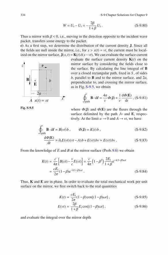
334 S-9 Chapter Solutions for Chapter 9
W = Ur−Ui = −2β
1+βUi . (S-9.80)
Thus a mirror with β < 0, i.e., moving in the direction opposite to the incident wave
packet, transfers some energy to the packet.
c) As a first step, we determine the distribution of the current density J. Since all
the fields are null inside the mirror, i.e., for x > x(t) = vt, the current must be local-
ized on the mirror surface, J(x, t)=K(t)δ(x−vt). We can evaluate the surface current
bE
xA x(t) = t
2a
B
z
Fig. S-9.5
evaluate the surface current density K(t) on the
mirror surface by considering the fields close to
the surface. By calculating the line integral of B
over a closed rectangular path, fixed in S , of sides
b, parallel to B and to the mirror surface, and 2a,
perpendicular to, and crossing the mirror surface,
as in Fig. S-9.5, we obtain
∮
path
B ·dℓ =4π
cΦ(J)+
1
c
dΦ(E)
dt, (S-9.81)
where Φ(J) and Φ(E) are the fluxes through the
surface delimited by the path Jv and E, respec-
tively. At the limit a→ 0 and A→ vt, we have
∮
path
B ·dℓ ≃ B(vt)b , Φ(J) = K(t)b , (S-9.82)
dΦ(E)
dt≃ ∂tE(vt) (vt−A)b+E(vt)bv ≃ E(vt)bv . (S-9.83)
From the knowledge of E and B at the mirror surface (Prob. 9.6) we obtain
K(t) =c
4π
[
B(vt)−v
cE(vt)
]
=c
4π
(
1−β2) 2Ei
1+βe−i(1−β)ωt
=cEi
2π(1−β)e−i(1−β)ωt . (S-9.84)
Thus, K and E are in phase. In order to evaluate the total mechanical work per unit
surface on the mirror, we first switch back to the real quantities
K(t) =cEi
2π(1−β)cos[(1−β)ωt] , (S-9.85)
E(vt) =2β
1+βEi cos[(1−β)ωt] , (S-9.86)
and evaluate the integral over the mirror depth

S-9.8 Pulse Modification by a Moving Mirror 335
∫ ∞
vt
J ·Edx =1
2K(t)E(vt) =
cE2i
2π
β(1−β)
1+βcos2[(1−β)ωt] . (S-9.87)
We have inserted the factor 1/2 to account for the discontinuity of E at x = vt (see
also Prob. 2.12). Equation (S-9.87) gives the mechanical power per unit surface
exerted on the mirror. To find the mechanical work, (S-9.87) must be integrated over
the time interval for which K(t) 0, i.e., for the time needed by the wave packet to
undergo a complete reflection. If the front of the wave packet reaches the mirror at
t = 0, the end of the packet will leave the mirror at t = τ/(1−β), which is different
from the pulse duration τ because the mirror moves while the wave train is reflected.
We thus need the integral
∫ τ/(1−β)
0
cos2[(1−β)ωt]dt =1
ω(1−β)
∫ ωτ
0
cos2 xdx =πN
(1−β)ω,
(S-9.88)
since ωτ = 2πN, and the integral of cos2 x over one period equals π. We thus obtain
W =
∫
1
2K(t)E(vt)dt =
cE2i
2π
β(1−β)
1+β
πN
(1−β)ω=
cE2i
4π
β
1+βτ (S-9.89)
= 2Iiτβ
1+β=
2β
1+βUi , (S-9.90)
in agreement with (S-9.80).
The work W. divided by the reflection time gives, the mechanical power per unit
surface
P =W1−β
τ=
2β(1−β)
1+βIi =
2(1−β)
1+βIi
v
c, (S-9.91)
which must be equal to the the pressure exerted on the moving mirror times its
velocity v. We thus obtain that the radiation pressure on a moving mirror is
Prad =P
v=
2Ii
c
1−β
1+β, (S-9.92)
a result which can also be obtained in different ways (see Problems
13.7 & 13.8).
S-9.9 Boundary Conditions on a Moving Mirror
a) We can assume the wave to be linearly polarized along y, without loss of gener-
ality. We choose the origin of the frame S ′, where the mirror is at rest, so that the
mirror surface is on the x′ = 0 plane. In S ′ the total fields at the mirror surface are

336 S-9 Chapter Solutions for Chapter 9
E′s(t′) = y′E′s(t
′) ≡ 0 ,
B′s(t′) = z′B′s(t
′)e−iω′it′ = −z′ 2E′i e−iω′
it′ , (S-9.93)
respectively, where
E′i = γ(1−β) Ei , ω′i = γ(1−β)ωi , (S-9.94)
are the amplitude and frequency of the incident wave in S ′, as seen in Problem 9.6.
Notice that E′ is continuous at x′ = 0, while B′ is not. By transforming the field
amplitudes at the mirror surface back to S we obtain
Es = γ(E′s+βB
′s) = γβB
′s = −2γ2β(1−β)Ei ,
Bs = γ(B′s−βE
′s) = γB′s = −2γ2(1−β)Ei , (S-9.95)
where β = v/c and γ = 1/√
1−β2. Thus, in general, in S we have both Es 0 and
Bs 0, while the fields are zero inside the mirror.
b) The EM fields are related to the vector potential by
E = −1
c∂tA , B = ∇×A. (S-9.96)
Thus, the only nonzero component of the vector potential is Ay, and we have
Es = −1
c∂tAy , Bs = ∂xAy . (S-9.97)
The total derivative of A appearing in (9.9) can be rewritten
dA
dt
∣
∣
∣
∣
∣
x=x(t)=[
∂tAy+ v∂xAy
]
x=x(t)= cEs− vBs = c (Es−βBs) = 0 , (S-9.98)
according to (S-9.95). Thus the equations (S-9.93) and (S-9.95) imply dA/dt
= 0 on the mirror surface in S .
c) The total vector potential in S is the sum of the vector potentials of the incident
and the reflected waves,
A(x, t) = y[
Ai eiki x−iωit +Are−ikr x−iωrt
]
= y[
Ai eiki(x−ct) +Ar e−ikr(x+ct)]
,
(S-9.99)

S-9.9 Boundary Conditions on a Moving Mirror 337
where Ai = icEi/ωi, ki = ωi/c, and kr = ωr/c. The boundary condition gives
0 = Ay(vt, t) = Ai e−iki(c−v)t +Ar e−ikr(c+v)t . (S-9.100)
This equation is satisfied if
Ar = −Ai ,kr
ki
=ωr
ωi
=c− v
c+ v=
1−β
1+β. (S-9.101)
For the total electric field we find
Ey = −1
c∂tAy = i
ωi
cAi eiki x−iωit − i
ωr
cAr e−ikr x−iωrt
= Ei eiki x−iωit −1−β
1+βEi e−ikr x−iωrt . (S-9.102)

Chapter S-10
Solutions for Chapter 10
S-10.1 Cyclotron Radiation
a) The electric dipole moment p = −er rotates in the xy plane with frequency ωL,
which is also the frequency of the emitted radiation. The dipole approximation is
valid if the dimensions of the radiating source are much smaller than the emitted
wavelength λ. Here this corresponds to the condition 2rL = 2v/ωL ≪ λ = 2πc/ωL,
always true for non-relativistic velocities.
The rotating dipole can be written as p = p0 (xcosωLt+ ysinωLt). For the electric
field of the dipole radiation observed in a direction of unit vector n, we have E ∝
−(p× n)× n. If n= z, then E∝ xcosωLt+ ysinωLt (circular polarization); if n= x or
n = y, we vave E ∝ −ysinωLt and E ∝ −xcosωLt, respectively (linear polarization).
Since r = v×ωL (where ωL = zωL), the radiated power can be written as
Prad =2
3
|er|2
c3=
2
3
e2v2ω2L
c3. (S-10.1)
b) We assume that the energy loss due to radiation is small enough to cause a vari-
ation of the orbit radius ∆rc ≪ rc during a single period, so that, during a single
period, the motion is still approximately circular. Thus the magnitude of the elec-
tron velocity v = v(t) can be written as v ≃ ωLr, where r = r(t) is the radius of the
orbit at time t. The electron energy is
U =mev2
2=
meω2Lr2
2, (S-10.2)
and the equation for the energy loss, dU/dt = −Prad, becomes
d
dt
(
meω2Lr2
2
)
= −2
3c3
(
e2ω4Lr2)
= −2remeω
4L
3cr2 , (S-10.3)
c© Springer International Publishing AG 2017
A. Macchi et al., Problems in Classical Electromagnetism,
DOI 10.1007/978-3-319-63133-2 23
339

340 Chapter S-10 Solutions for Chapter 10
where re = e2/(me c2) is the classical electron radius. Substituting the relation
d(r2)/dt = 2r dr/dt into (S-10.3) we obtain
dr
dt= −
2reω2L
3cr ≡ −
r
τ, with τ =
3c
2reω2L
=3mec3
2e2ω2L
, (S-10.4)
whose solution is
r(t) = r(0)e−t/τ , (S-10.5)
and the trajectory of the electron is a spiral with a decay time τ. Inserting the expres-
sions for re and ωL we have
τ =3
2
m3ec5
e4B20
=5.2×10⁵
B20
s (S-10.6)
where the magnetic field B0 is in G. The condition τ≫ ω−1L implies
3
2
m3ec5
e4B20
≫mec
eB0, or B0≪
3
2
m2ec4
e3= 9.2×10¹³ G , (S-10.7)
a condition well verified in all experimental conditions: such high fields can be
found only on neutron stars! (see Problem 10.5)
c) We insert a frictional force ffr = −meηv into the equation of motion, obtaining
medv
dt= −
e
cv×B0−meηv . (S-10.8)
This corresponds to the following two coupled equations for the the x and y compo-
nents the electron velocity
vx = −ωLvy−ηvx , vy = ωLvx −ηvy . (S-10.9)
An elegant method to solve these equations is to combine the x and y coordinates of
the electron into a single complex variable R = x+ iy, and the velocity components
into the complex variable V = vx+ ivy. The two equations (S-10.9) are thus combined
into the single complex equation
V = (iωL−η)V , with solution V = V(0)eiωLt−ηt = v0 eiωLt−ηt . (S-10.10)
For the electron position we have
R =
∫
V dt+C =v0
iωL−ηeiωLt−ηt +C = −
(η+ iωL)v0
ω2L+η2
eiωLt−ηt +C , (S-10.11)

S-10.1 Cyclotron Radiation 341
where C is a complex constant depending on our choice of the origin of the coordi-
nates. We choose C = 0, and rewrite (S-10.11) as
R = −v0
√
ω2L+η2
(cosφ+ i sinφ)eiωLt−ηt = −v0
√
ω2L+η2
ei(ωLt+φ)−ηt , (S-10.12)
where
cosφ =η
√
ω2L+η2
, sinφ =ωL
√
ω2L+η2
, φ = arctan
(
ωL
η
)
. (S-10.13)
Going back to the real quantities we have
vx = Re(V) = v0 e−ηt cosωLt , (S-10.14)
vy = Im(V) = v0 e−ηt sinωLt , (S-10.15)
x = Re(R) = −v0
√
ω2L+η2
e−ηt cos(ωLt+φ) , (S-10.16)
y = Im(R) = −v0
√
ω2L+η2
e−ηt sin(ωLt+φ) . (S-10.17)
Thus, the velocity rotates with frequency ωL, while its magnitude decays exponen-
tially, |v(t)| = v0 e−ηt. For the radius of the trajectory we have
r(t) = |R(t)| =v0
√
ω2L+η2
e−ηt . (S-10.18)
Thus, choosing η = 1/τ, the motion with frictional force is identical to the motion
with radiative power loss, and
ffr · v = −meηv2 = −
mev2
τ= −mev2 2e2ω2
L
3mec3= −
2e2v2ω2L
3c3= −Prad . (S-10.19)
A drawback of this approach is that the frictional coefficient inserted here is
not universal but is dependent on the force on the electron (in this case, via the
dependence on ωL). See Problem 10.12 for a more general approach to radiation
friction.

342 Chapter S-10 Solutions for Chapter 10
S-10.2 Atomic Collapse
a) An electron describing a circular orbit of radius a0 (Bohr radius) around a proton
corresponds to a counterrotating electric dipole p(t) of magnitude p0 = ea0. The
angular velocity of the orbit ω can be evaluated by considering that the centripetal
acceleration is due to the Coulomb force,
ω2a0 =1
me
e2
a20
, (S-10.20)
from which we obtain
ω =
√
e2
mea30
= 4.1×10¹⁶ rad/s . (S-10.21)
Actually, the strongest emission from the hydrogen atom occurs at a frequency
smaller by about one order of magnitude.
Since p is perpendicular to ω, we have p = (p×ω)×ω and |p|2 =(
ω2 p0
)2(the
same result can be obtained by considering the rotating dipole as the superposition
of two perpendicularly oscillating dipoles). Thus the radiated power is
Prad =2
3c3|p|2 =
2
3
ω4e2a20
c3=
2
3
e2r2e c
a40
, (S-10.22)
where re is the classical electron radius.
b) We assume that, due to the emission of radiation, the electron loses its energy
according to dU/dt = −Prad, where U = K +V is the total electron energy, K and V
being the kinetic and potential energy, respectively. If the energy lost per period is
small with respect to the total energy, we may assume that the electron the orbit is
almost circular during a period, with the radius slowly decreasing with time, r = r(t)
with r/r≪ ω.
Since the velocity is v = rω, the total energy can be written as a function of a:
U = K +V =mev2
2−
e2
r= −
e2
2r. (S-10.23)
Therefore
dU
dt≃ −
e2
2
d
d
(
1
r
)
=e2
2r2
dr
dt. (S-10.24)
S-10.2 Atomic Collapse 343
Since
Prad =2
3
e2r2e c
r4(S-10.25)
the equation dU/dt = −Prad can be written as
e2
2r2
dr
dt= −
2
3
e2r2e c
r4⇒ r2 dr
dt= −
4
3r2
e c ⇒1
3
dr3
dt=
4
3r2
e c (S-10.26)
The solution, assuming r(0) = a0, is
r3 = a30−4r2
e c t , (S-10.27)
giving for the time need by the electron to fall on the nucleus
τ =a3
0
4r2e c≃ 1.6×10⁻¹¹ s . (S-10.28)
This is a well-known result, showing that a classical “Keplerian” atom is not stable.
It is however interesting to notice that the value of τ is of the same order of mag-
nitude of the lifetime of the first excited state, i.e., of the time by which the excited
state decays to the ground state emitting radiation.
S-10.3 Radiative Damping of the Elastically Bound Electron
a) The solution of (10.5) with the given initial conditions and η = 0 is
r = s0 cosω0t . (S-10.29)
The corresponding average radiated power in the dipole approximation is
Prad =2
3c3
⟨
−e|r|2⟩
=2e2
3c3ω4
0s20
⟨
cos2ω0t⟩
=e2
3c3ω4
0s20 . (S-10.30)
The radiated power is emitted at the expense of the energy of the oscillating elec-
tron. Thus, the total mechanical energy of electron must decrease in time, and the
harmonic-oscillator solution of (S-10.29) cannot be exact. Assuming that the energy
of the oscillator decays very slowly, i.e., with a decay constant τ ≫ ω−10
, we can
approximate (S-10.29) as
r ≃ s(t)cosω0t . (S-10.31)
344 Chapter S-10 Solutions for Chapter 10
where s(t) is a decreasing function of time to be determined. Consequently, we must
replace s0 by s(t) also in equation (S-10.30) for the actual average radiated power.
b) At time t, the total energy of the oscillating electron is U(t) = meω20s2(t). The
time decay constant τ is defined as
τ =U(t)
Prad(t)=
3mec3
2e2ω20
=3c
2reω20
, (S-10.32)
and is thus independent of t. Since the classical electron radius is re ≃ 2.82×10⁻¹⁵ m,
the condition τ > 2π/ω0 leads to
ω0 <3
4π
c
re≃ 3×10²² rad/s . (S-10.33)
For a comparison, estimating ω0 as the frequency of the 1S←2P Lyman-alpha emis-
sion line of the hydrogen atom, we have ω0 ≃ 3×10¹⁶ rad/s.
c) We look for a solution of the form r = Re(s0 e−iωt), with complex ω. Substituting
this into (10.5), the characteristic equation becomes
ω2+ iηω+ω20 = 0 , (S-10.34)
whose solution is
ω = −iη
2±
√
ω20−η2
4≃ −iη
2±ω0 , (S-10.35)
where we have neglected the terms of the order (η/ω0)2 and higher. Thus, the
approximated solution for the electron position is
r ≃ s0 e−ηt/2 cosω0t . (S-10.36)
Actually, this approximation gives an initial velocity r(0) = −ηs0/2 instead of zero.
However, this discrepancy can be neglected if η≪ω0. The maximum speed reached
by the electron is vmax ≃ ω0s0, and ηs0/2≪ ω0s0.
The time-dependent total energy of the electron and average radiated power are
U(t) ≃me
2ω2
0s20 e−ηt , and Prad(t) ≃
e2
3c3ω4
0s20 e−ηt . (S-10.37)
The condition dU/dt = −Prad leads to
η =2reω
20
3c=
1
τ. (S-10.38)

S-10.4 Radiation Emitted by Orbiting Charges 345
S-10.4 Radiation Emitted by Orbiting Charges
a) Let us denote by r1 and r2 the location vectors of the two charges with respect to
the center of their common circular orbit. In polar coordinates we have
r1 ≡[
R,φ1(t)]
, and r2 ≡[
R,φ2(t)]
. (S-10.39)
Defining ∆φ = φ2 −φ1 and choosing an appropriate origin of time, the equations of
motion in polar coordinates are
r1 ≡
(
R,ωt−∆φ
2
)
, and r2 ≡
(
R,ωt+∆φ
2
)
. (S-10.40)
In Cartesian coordinates we have
r1 ≡[
x1(t),y1(t)]
, and r2 ≡[
x2(t),y2(t)]
, (S-10.41)
with, respectively,
x1(t) = Rcos
(
ωt−∆φ
2
)
, y1(t) = Rsin
(
ωt−∆φ
2
)
, (S-10.42)
x2(t) = Rcos
(
ωt+∆φ
2
)
, y2(t) = Rsin
(
ωt+∆φ
2
)
. (S-10.43)
The dipole moment of the system is p = q(r1+ r2), with Cartesian components
px = qR
[
cos
(
ωt−∆φ
2
)
+ cos
(
ωt+∆φ
2
)]
= 2qRcos
(
∆φ
2
)
cosωt , (S-10.44)
py = qR
[
sin
(
ωt−∆φ
2
)
+ sin
(
ωt+∆φ
2
)]
= 2qRcos
(
∆φ
2
)
sinωt , (S-10.45)
i.e., p has constant magnitude p = 2qRcos(∆φ/2), and rotates in the z = 0 plane with
angular frequency ω.
b) In the dipole approximation, the electric field of the radiation emitted along a
direction of unit vector the n is parallel to the vector
(p× n)× n = p⊥ . (S-10.46)
Since for a dipole rotating in the z = 0 plane
(p× x)× x is parallel to y , and (p× y)× y is parallel to x , (S-10.47)
the polarization of the radiation observed in the x (y) direction is linear and along y
(x). For radiation observed the z direction

346 Chapter S-10 Solutions for Chapter 10
(p× z)× z is parallel to p , (S-10.48)
and the observed polarization is circular.
The total radiated power is
Prad =2
3c3|p|2 =
4q2R2ω4
3c3cos2
(
∆φ
2
)
, (S-10.49)
which obviously vanishes when p = 0, i.e., for ∆φ = π (charges on opposite ends of
a rotating diameter), and has a maximum for ∆φ = 0 (superposed charges).
c) In this case charges are superposed to each other every half turn. We choose the
coordinates and the time origin so that the charges are superposed at t = 0 we have
r1 = r2 = (R,0). Thus the trajectories can be written as
r1 = r2 = R , φ1(t) = ωt , φ2(t) = −ωt , (S-10.50)
in polar coordinates, and as
x1(t) = Rcosωt , y1(t) = Rsinωt ,
x2(t) = Rcosωt , y2(t) = −Rsinωt , (S-10.51)
in Cartesian coordinates. The total dipole moment is thus p = (2qRcosωt) x. No
radiation is emitted along x, while the radiation emitted along all other directions is
linearly polarized. The total average radiated power is
Prad =2
3c3|p|2 =
4q2R2ω4
3c3. (S-10.52)
d) With an appropriate choice of the time origin the equations of motion of the three
charges can be written, in polar coordinates, as
r1 = r2 = r3 = R , φ1(t) = ωt ,
φ2(t) = ωt+∆φ2 , φ3(t) = ωt+∆φ3 , (S-10.53)
and, in Cartesian coordinates,
xi = Rcosφi(t) , yi = Rsinφi(t) , (i = 1,2,3) . (S-10.54)
The electric dipole moment vanishes if the three charges are on the vertices of a
rotating equilateral triangle (∆φ2 = −∆φ3 = 2π/3), and has its maximum value when
the three charges are overlapped (∆φ2 = ∆φ3 = 0).
e) The magnetic dipole moment for a point charge q, traveling at angular velocity ω
on a circular orbit of radius R, is defined by

S-10.4 Radiation Emitted by Orbiting Charges 347
m =1
2c
∫
r×Jd3x =qR2ω
2c, (S-10.55)
and is constant (notice that m is proportional to the angular momentum of the orbit-
ing charge). Thus the magnetic dipole does not contribute to radiation, because the
radiation fields are proportional to m.
This problem explains why a circular coil carrying a constant current does not
radiate, although we may consider the current as produced by charges moving on
circular orbits, and thus subject to acceleration.
S-10.5 Spin-Down Rate and Magnetic Field of a Pulsar
a) Due to the nonzero angle α between the magnetic moment and the rotation axis
of the pulsar, the component of m perpendicular toω rotates with frequency ω. Thus
the Pulsar emits magnetic dipole radiation of frequency ω. The total power is
P =2
3c3|m⊥|
2 =2
3
m2⊥ω
4
c3, (S-10.56)
where m⊥ = msinα.
b) The mechanical energy is U = Iω2/2, where I = 2MR2/5 ≃ 1.1× 1043 g cm2 is
the moment of inertia of the pulsar, assuming a uniform mass distribution over the
volume of a sphere of radius R. Assuming that the energy loss is due to radiation
emission only, we can write
dU
dt=
d
dt
(
Iω2
2
)
= Iωω = −P , (S-10.57)
and, substituting (S-10.56), we have
Iωω = −2
3
m2⊥ω
4
c3⇒
ω
ω3= −
2m2⊥
3Ic3. (S-10.58)
By integrating over time from 0 to t we obtain
1
2ω2(t)−
1
2ω2(0)=
2m2⊥
3Ic3t , (S-10.59)
and thus
ω(t) =ω(0)√
1+t
τ
, where τ =3Ic3
4m2⊥ω
2(0). (S-10.60)

348 Chapter S-10 Solutions for Chapter 10
c) We can rewrite ω/ω3 as ω/ω3 = −TT/4π2, where T = 2π/ω is the rotation period
of the pulsar, and T = −2πω/ω2. Thus we can obtain the magnetic dipole moment
m =m⊥ of the pulsar as a function of the experimentally measured parameters from
(S-10.58):
m =
√
3Ic3
8π2TT ≃ 3.3×1036
√
TT erg/G , (S-10.61)
where T is in seconds. The magnetic field immediately outside of the pulsar surface
is the field of a magnetic dipole located at the pulsar center:
B =3(r ·m) r−m
r3, (S-10.62)
and thus Bmax = 2m/R3. Thus we obtain the practical formula
Bmax ≃ 6.6×10²¹√
TT G , (S-10.63)
Inserting the experimental values for T and T we obtain
Bmax ≈ (9.6±0.25)×1016 G . (S-10.64)
S-10.6 A Bent Dipole Antenna
a) If we divide the antenna into a series of infinitesimal resistors, each of length dz
and resistance dR = (R/a)dz, we can write the dissipated power as
Pdiss =
∫
〈I2〉dR =
∫
+a
−a
I20
2
(
1−|z|
a
)2R
adz =
I20R
3. (S-10.65)
b) The linear charge density on the antenna qℓ can be obtained from the continuity
equation ∂tqℓ = −∂zI, obtaining
qℓ = ±iI0
aωe−iωt, (S-10.66)
where the signs + and − apply to z > 0 and z < 0, respectively. The linear charge
density is uniform (independent of z) on each half of the antenna. For symmetry
reasons, the only non-vanishing component of the electric dipole p is along z and it
is given by
pz =
∫ +a
−a
zqℓ dz = 2
∫ +a
0
iI0
aωe−iωtzdz =
iI0 a
ωe−iωt . (S-10.67)

S-10.6 A Bent Dipole Antenna 349
c) The average radiated power, in the dipole approximation, is
Prad =1
3c3
⟨
|pz|2⟩
=I20a2ω2
6c3=
2π2a2I20
3cλ2, (S-10.68)
where λ = 2πc/ω is the radiation wavelength. Thus
Prad
Pdiss
=2π2a2
cλ2R, (S-10.69)
where we recall that R has the dimensions of the inverse of a velocity in Gaussian
units.
d) The angular distribution of the radiated power is proportional to sin2 θ, where
θ is the angle between the observation direction and p. Thus the emitted radiation
intensity is zero along the z axis and maximum for observation in the xy plane.
e) The bent antenna has a linear charge density ±(iI0/aω)e−iωt on its horizontal and
vertical arms, respectively. Thus the electric dipole moment has two components
px =
∫ a
0
iI0
aωe−iωt xdx =
iI0a
2ωe−iωt , (S-10.70)
pz = −
∫ 0
−a
iI0
aωe−iωtzdz =
iI0a
2ωe−iωt . (S-10.71)
Since the components are perpendicular to each other, the cycle-averaged radiated
power can be calculated as the sum of the powers from each dipole:
Prad =1
3c3
⟨
|px|2+ |pz|
2⟩
=1
12c3(I0ωa)2 , (S-10.72)
which is one half of the value for the linear antenna, while the dissipated power Pdiss
does not change.
The electric dipole of the bent antenna lies along the diagonal direction, which
thus corresponds to the direction of zero emitted intensity. The intensity is maximum
in the plane perpendicular to the dipole.
S-10.7 A Receiving Circular Antenna
a) We choose a Cartesian reference frame such that the wave is propagating in
the z direction, its electric field E is along the x axis, and its magnetic field B
is along the y axis. The current I flowing in the antenna is I = Ecirc/R, where
Ecirc = −(1/c)dΦ(B)/dt is the electromotive force, andΦ(B) is the flux of B through
the circle delimited by the antenna. Since we have assumed λ≫ a, B is practically
uniform over the whole surface of the circle, and Φ(B) ≃ πa2B · n, where n is unit

350 Chapter S-10 Solutions for Chapter 10
vector perpendicular to the circle surface. Thus the circular antenna must lie on the
xz plane in order to maximize Φ(B). With a proper choice of the time origin the
magnetic field on the circle surface can be written as B ≃ y B0 cosωt, and
Ecirc = πa2ω
cE0 sin(ωt) , (S-10.73)
since B0 = E0 in Gaussian units.
b) The electromotive force on a linear antenna parallel to the x axis is practically
Elin = ℓE0 cos(ωt+φ), where ℓ is rhe length of the antenna and φ is a phase angle.
The ratio of the average electromotive force of the circular antenna to the average
electromotive force of the linear antenna is thus
〈Ecirc〉
〈Elin〉≃〈Ecirc〉
E0ℓ=πa2ω
ℓc= 2π2 a2
ℓλ. (S-10.74)
In the range 102 cm<λ< 103 cm, and with our assumptions ℓ≃ 50cm and a≃ 25cm,
this ratio varies between 2.5 and 0.25. The circular antenna is more convenient for
shorter wavelengths.
c) The radiation emission from the circular antenna is dominated by the magnetic
dipole term. The dipole moment of the antenna is
m =1
cIπa2 n , (S-10.75)
where I is the current circulating in the antenna due to the electromotive force
induced by the incident wave. The corresponding time-averaged radiated power is
Prad =2
3c3
⟨
|m|2⟩
=2
3c5(πa2)2ω4
⟨
I2⟩
=(πa2)4ω6
3c7R2E2
0 . (S-10.76)
In Gaussian units, the intensity of the incoming wave is I = cE20/4π, and (S-10.76)
can be rewritten
Prad =4π(πa2)4ω6
3c8R2I =
2(2π)7(πa2)4
3c2R2λ6I . (S-10.77)
The factor multiplying I,
σscatt =2(2π)7(πa2)4
3c2R2λ6, (S-10.78)
has the dimensions of a surface (R has the dimensions of an inverse velocity in
Gaussian units), and is the radiative scattering cross section for our circular antenna,
in the magnetic dipole approximation.

S-10.7 A Receiving Circular Antenna 351
The time-averaged power dissipated by Joule heating is Pdiss = R〈I2〉, so that
Prad
Pdiss
=2
3c5R(πa2)2ω4 =
2(2π)4(πa2)2
3Rcλ4. (S-10.79)
S-10.8 Polarization of Scattered Radiation
a) We choose a Cartesian reference frame with the origin located on the scattering
particle, and the z axis parallel to the wave vector of k the incident wave. In order to
have complete rotational symmetry around the z axis it is convenient to assume that
the incident wave is circularly polarized. The electric field of the incoming wave
can thus be written
Ei = E0(x± iy)eikz−iωt . (S-10.80)
Thus, the dipole moment of the scatterer is p = αEi = αE0(x± iy)eikz−iωt.
z
θ
y
y
kkd
z
Fig. S-10.1
Because of the rotational symme-
try of the problem around the z axis,
it is sufficient to consider the scat-
tered radiation with the wave vector
kd lying in the yz plane and forming
an angle θ with the z axis, as shown
in Fig. S-10.1. Disregarding a propor-
tionality factor depending on α and θ,
the electric field Ed of the scattered
radiation can be written
Ed ∝ −(p× n)× n
∝ −[(x± iy)× n]× n , (S-10.81)
where n = (0,sinθ,cosθ) is the unit vector parallel to kd. Now, recalling that
(x± iy)× n = (±i cosθ,−cosθ,sinθ) , (S-10.82)[
(x± iy)× n]
× n = (−1,∓i cos2 θ,±i sinθcosθ) , (S-10.83)
we fint that
Ed ∝(
1, ±i cos2 θ, ∓i sinθcosθ)
. (S-10.84)
Since an observer would measure the polarization of the scattered radiation with
respect to the direction n, we calculate the components of the field in the rotated

352 Chapter S-10 Solutions for Chapter 10
coordinate system (x′,y′,z′), rotated by an angle θ around the x axis, so that x′ = x
and z′ is along n:
E′d x = Ed x ∝ 1 , (S-10.85)
E′dy = Edy cosθ−Edz sinθ ∝ ±Ii cos3 θ± i sin2 θcosθ
= ±i cosθ(
cos2 θ+ sin2 θ)
= ±i cosθ , (S-10.86)
E′dz = Edy sinθ+Edz cosθ ∝ ±i sinθcos2 θ∓ i sinθcos2 θ = 0 . (S-10.87)
The last equality is a check that the radiation field is transverse. We thus obtain
Ed ∝ x′± i cosθ y′ , (S-10.88)
which gives the dependence of the polarization on the scattering angle θ. In addition,
the angular distribution or the radiated power is given by
dPscatt
dΩ∝ |Ed|
2 ∝ 1+ cos2 θ . (S-10.89)
b) The radiation from most sources (sunlight is a typical example) is usually inco-
herent. This means that its phase and electric field direction change randomly at
time intervals not much longer than the oscillation period. Thus, the radiation is
effectively unpolarized at direct observation, in the sense that it is not possible to
measure a definite polarization because of its fast variations. However, (S-10.88)
shows that, independently of the source polarization, the radiation scattered at 90
(cosθ = 0) is always linearly polarized (in the direction perpendicular to both the
wave vector of the incoming light and the observation direction). Hence, incoher-
ent radiation that has undergone scattering (as the blue light from the sky) tends to
be polarized, even if the radiation from the primary source (in this case the sun)
is unpolarized. A measurement of the polarization might help, then, to localize the
position of the Sun on a cloudy day.
S-10.9 Polarization Effects on Thomson Scattering
a) Equation (10.7) leads to the following two equations for the velocity components
of the electron, vx and vy,
mevx = −eE0 cosθcos(kz−ωt) , mevx = −eE0 sinθ sin(kz−ωt) , (S-10.90)

S-10.9 Polarization Effects on Thomson Scattering 353
where me is the electron mass. We search for a steady-state solution of the form
vx = V0x sin(kz−ωt) , vy = V0y cos(kz−ωt) , (S-10.91)
with V0x and V0y two real constants to be determined. Substituting into (S-10.90)
we obtain
V0x =eE0 cosθ
meω, V0y = −
eE0 sinθ
meω. (S-10.92)
The second derivative of the electric dipole moment of the electron with respect to
time is
p = −ev = −e2E0
me
[
(xcosθcos(kz−ωt)+ ysinθ sin(kz−ωt)]
, (S-10.93)
and the electron radiates at frequency ω. The polarization for scattered radiation
propagating in a generic direction of unit vector n direction is parallel to the projec-
tion of the dipole moment onto the plane perpendicular to n, i.e., to p⊥ = (p× n)× n.
Thus, we observe linear polarization parallel to y for the radiation emitted along x,
and linear polarization parallel to x for the radiation emitted along y, and elliptical
polarization for the radiation emitted along z.
If 0 < θ < π/4, so that sinθ < cosθ, we choose the observation-direction unit
vector n = (sinψ,0,cosψ), lying in the xz plane, and forming an angle ψ with the z
axis, as shown in Fig. S-10.2, where ki is the wave vector of the incident wave. Now
we choose a Cartesian reference frame x′,y′,z′, with y′ ≡ y and z′ along n, so that
the scattered radiation of interest is propagating along z′.
ki
n
xcos θ
sinθ
y y
x
zz
Fig. S-10.2
If we perform an orthogonal projection onto the
x′y′ plane of an ellipse lying on the xy plane, of
half axes cosθ parallel to x, and sinθ parallel to
y, we obtain an ellipse of half-axes cosθcosψ
along x′, and sinθ along y′. Thus we observe
a circular polarization if cosθcosψ = sinθ, i.e.,
if cosψ = tanθ. Analogously, if π/4 < θ < π/2,
so that sinθ > cosθ, we choose the observation-
direction unit vector n = (0,sinψ,cosψ), lying in
the yz plane, and we observe circular polarization
if sinθcosψ = cosθ, i.e., if cosψ = cotθ . b) The
average total scattered power is
P =2
3c3
⟨
|p|2⟩
=2e4
3m2ec3
⟨
|E|2⟩
, (S-10.94)

354 Chapter S-10 Solutions for Chapter 10
where
⟨
|E|2⟩
=⟨
E2x +E2
y
⟩
=1
2E2
0
(
cos2 θ+ sin2 θ)
=1
2E2
0 . (S-10.95)
Thus, the total scattered power is independent of θ and can be written as
P =e4E2
0
3m2ec3=
cE20
3r2
e =4π
3r2
e I , (S-10.96)
where
re =e2
mec2, and I =
cE20
4π,
are the classical electron radius and the intensity of the incident wave, respectively.
c) The magnetic field of the wave is
B = E0[
−xsinθ sin(kz−ωt)+ ycosθcos(kz−ωt)]
. (S-10.97)
The only non-vanishing component of v×B is in the z direction, and the magnetic
force on the electron can be written as
Fz = −e
c(v×B)z = −
e
c(vxBy− vyBx)
= −e2E2
0
2cmeω(cos2 θ− sin2 θ) sin(2kz−2ωt) , (S-10.98)
this quantity vanishes for θ = π/4, when cosθ = sinθ, i.e., for circular polarization.
d) The magnetic force Fz drives dipole oscillations along the z axis at frequency
2ω. Thus, in addition to the scattered radiation of frequency ω discussed at points a)
and b), we observe also scattered radiation of frequency 2ω, angularly distributed
as sin2ψ around the z axis. Since the dipole oscillating at 2ω is perpendicular to the
dipole oscillating at ω, we can simply add the corresponding scattered powers. Now
we want to evaluate the power emitted at frequency 2ω.
The equation of motion for the electron along the z axis is (we put cos2 θ−sin2 θ =
cos2θ)
mevz = Fz = −e2E2
0
2cmeωcos2θ sin(2kz−2ωt) . (S-10.99)
Once more, we search for a steady-state solution of the form
vz = V0z cos(2kz−2ωt) , (S-10.100)
with V0z a constant. Substituting into (S-10.99) we obtain

S-10.9 Polarization Effects on Thomson Scattering 355
V0z = −e2E2
0
4cm2eω
2cos(2θ) (S-10.101)
and
vz = −e2E2
0
2cm2eω
cos(2θ) sin(2kz−2ωt) . (S-10.102)
The total average power emitted by the dipole oscillating at 2ω is
P2ω =2
3c3
⟨
∣
∣
∣p2ω
∣
∣
∣
2⟩
=2
3c3
⟨
|evz|2⟩
=e6E4
0
12c5m4eω
2cos2(2θ)
=4π
3
e2E20
4c2m2eω
2cos2(2θ)r2
e I
=4π
3
V0z
ccos2(2θ)r2
e I . (S-10.103)
S-10.10 Scattering and Interference
a) With a proper choice of the time origin, the electric field of the incident plane
wave at x = ±d/2 can be written as
Ei
(
±d
2, t
)
= E0 e±ikd/2−iωt z , (S-10.104)
and the phase difference between the two scatterers is
φ+−φ− = kd . (S-10.105)
We denote by r± the optical paths between the observation point P and the scatterers
located at (±d/2,0,0), as shown in Fig. 10.5. The difference between the two optical
paths is
∆r = (r+− r−) ≃ −d sinθ , (S-10.106)
where θ is the angle between the y axis and the line joining the origin to P, as shown
in Fig. 10.5. The approximation is valid for L≫ d. The phase difference between
the two scattered waves in P is obtained by combining (S-10.105) and (S-10.106),
∆φ = kd(1− sinθ) . (S-10.107)
b) If we neglect the difference between the magnitudes of the scattered fields E+ and
E− in P, E± being the field of the wave scattered at (±d/2,0,0), the total scattered
intensity Is in P is proportional to

356 Chapter S-10 Solutions for Chapter 10
Is ∝ |E++E−|2 ∝ |E+|
2∣
∣
∣eikd(1−sinθ)/2+ e−ikd(1−sinθ)/2∣
∣
∣
2
∝1
r2cos2
[
kd
2(1− sinθ)
]
. (S-10.108)
Since r cosθ = L, we can also write
Is ∝cos2 θ
L2cos2
[
kd
2(1− sinθ)
]
. (S-10.109)
We denote by u = (kd/2)(1− sinθ) the argument of the second cos2 appearing in
(S-10.109). For −π/2 θ π/2 the variable u varies continuously and monotonically
from kd to 0. If kd ≪ 1 (i.e., if d ≪ λ/2π), then cos2 u ≃ 1 e Is(θ) ∼ cos2 θ, as if a
single scatterer was present. If kd < π/2 the function cos2 u has no zeros, meaning
that interference fringes are not observed if the distance between the scatterers is
less than λ/4. Ifπ
2<
kd
2< (n+1)
π
2,
with n an integer number and n 1, the function cos2 u has n zeros, and one observes
n scattered-intensity minima and n+1 maxima as θ varies from −π/2 to +π/2. The
intensity of the maxima is modulated by the function cos2 θ.
S-10.11 Optical Beats Generating a “Lighthouse Effect”
a) On the z = 0 plane the electric fields E± emitted by the two dipoles are parallel
to z (perpendicular to the plane), and their amplitudes are independent of φ. Since
for each dipole E± ∝ −ω2±p0, the field amplitudes are E+ ≃ E−, equal to each other
up to the first order in δω/ω0. The difference between the optical paths from the two
dipoles to P is δr ≃ d sinφ = (πc/ω0) sinφ, which yields a phase difference of πsinφ.
The total field may be thus written as
E = E0 cos[(ω0+δω/2)t+πsinφ/2]+E0 cos[(ω0−δω/2)t−πsinφ/2]
= 2E0 cos(ω0t)cos(δωt+πsinφ) . (S-10.110)
b) The EM energy flux in the radiation zone is given by Poynting’s vector S, which
is proportional to the square modulus of the electric field. Thus
S ∝ 4cos2(ω0t)cos2(δωt+πsinφ). (S-10.111)
Using the “fast”, or “instantaneous”, detector, only the factor cos2(ω0t) is averaged,
and the measured signal is proportional to
〈S 〉 ∝ 2cos2(δωt+πsinφ) , since⟨
cos2(ω0t)⟩
=1
2. (S-10.112)

S-10.11 Optical Beats Generating a “Lighthouse Effect” 357
At time t, the direction of maximum flux intensity is determined by the condition
δωt+πsinφ =
0
π, (S-10.113)
which means that the direction of maximum flux φmax rotates in the z = 0 plane,
similarly to a lighthouse beam, according to
φmax(t) = arcsin
(
−δω
πt
)
. (S-10.114)
p− p+
P
O
z
yx
r
θ
Fig. S-10.3
If the EM flux is measured with the “slow” detector,
i.e., averaging over times longer than 2π/δω, both
cos2 terms of (S-10.111) are averaged to 1/2, and
the total flux is the sum of the two independent fluxes
from the two dipoles.
c) Now the observation point P is on the x = 0 plane,
at a distance r from the origin, as in Fig. S-10.3.
The angle between the z axis and r is θ. Within our
approximations, the intensities of the two electric
fields E+ and E− in P are equal and proportional to
sinθ. Thus the two separate intensities are dependent
on θ, while they are independent of φ on the z = 0 plane. The amplitude of the
Poynting vector is proportional to
S ∝ 2sin2 θcos2(ω0t)cos2(δωt+πsinθ) . (S-10.115)
Thus the “fast” detector still measures a rotation of the direction of maximum emis-
sion, but the intensity is modulated by a sin2 θ factor.
S-10.12 Radiation Friction Force
a) We insert (10.11) for Frad into (10.9), obtaining
∫ t+T
t
Frad(t) · v(t)dt = meτ
∫ t+T
t
d2v(t)
dt2· v(t)dt
= meτ
[
dv(t)
dt· v(t)
]t+T
t
−meτ
∫ t+T
t
∣
∣
∣
∣
∣
dv(t)
dt
∣
∣
∣
∣
∣
2
dt , (S-10.116)

358 Chapter S-10 Solutions for Chapter 10
where we have used integration by parts in the second line. The first term vanishes
since the motion is periodic1:
[
dv(t)
dt· v(t)
]t+T
t
=1
2
[
d
dtv
2(t+T )−d
dtv
2(t)
]
= 0 . (S-10.117)
We thus obtain
∫ t+T
t
Frad(t) · v(t)dt = −meτ
∫ t+T
t
∣
∣
∣
∣
∣
dv
dt
∣
∣
∣
∣
∣
2
dt . (S-10.118)
Substituting Larmor’s formula (10.10) into the right-hand side of (10.9) we obtain
−
∫ t
0
Prad(t′)dt′ = −
∫ t
0
2e2
3c2
∣
∣
∣
∣
∣
dv
dt′
∣
∣
∣
∣
∣
2
dt′ , (S-10.119)
and (10.9) is verified if we choose
τ =2e2
3mec2. (S-10.120)
Apart from the 2/3 factor, τ is the time needed by light to travel a distance equal to
the classical electron radius re = 2.82×10⁻¹³ cm, and we have τ ∼ 10−23 s.
b) After substituting (10.12) into (10.8), we search for a steady-state solution of the
form v(t) = v0 e−iωt, and find
v0 = −ieE0
meω(1+ iωτ). (S-10.121)
Analogously, the steady-state solution of (10.13) is
v0 = −ieE0
meω
(
1+ iη
ω
) . (S-10.122)
The two solutions are identical if we choose η = ω2τ. The same result can be
obtained by a direct comparison of Frad to the frictional force −meηv.
Equation (10.8) represents the first attempt to derive an expression for the “radia-
tion friction” or “radiation reaction” force which is deeply related to the back-action
of the electron on itself, since the electron interacts with the electric field it gener-
ates (self-force9. However. (10.8) is considered unsatisfactory for for two reasons:
(i) it increases the order of the equation of motion, and, consequently, one needs
a further initial condition for the acceleration; and ii) it has unphysical “runaway”
1Actually it is not strictly necessary for the motion to be periodic, it is sufficient that dv2(t)dt
vanishes at the initial and final instants of the time interval considered.

S-10.12 Radiation Friction Force 359
solutions in the absence of an external field, such as a(t) = a0 et/τ with a = dv/dt.
This problem has a long and still open history. Additional discussion may be found
in textbooks and in the literature, also in very recent works related to highly rela-
tivistic electrons in ultraintense laser fields (for which the radiation friction effect
becomes important).

Chapter S-11
Solutions for Chapter 11
S-11.1 Wave Propagation in a Conductor at High and Low
Frequencies
a) We determine the conductivity of the metal by searching for a steady-state solu-
tion in complex form, v = ve−iωt, of (11.5) in the presence of an oscillating electric
field E(r, t) = Ee−iωt. We find
v = − ie
me(ω+ iη)E , (S-11.1)
corresponding to a current density
J = −ene v =ie2ne
meω(ω+ iη)E =
iω2p
4π(ω+ iη)E ≡ σ(ω) E , (S-11.2)
where ωp is the plasma frequency of the metal. At the limits of high frequencies
ω≫ η, and of low frequencies ω≪ η, we have
σ(ω) ≃
⎧
⎪
⎪
⎪
⎪
⎪
⎪
⎪
⎪
⎪
⎨
⎪
⎪
⎪
⎪
⎪
⎪
⎪
⎪
⎪
⎩
iω2p
4πω, for ω≫ η ,
ω2p
4πη, for ω≪ η .
(S-11.3)
The DC conductivity is thus σDC = σ(0) = ω2p/4πη. In a metal, typically we have
ωp ∼ 1016 s−1, since ne ∼ 1023 cm−3 and η ∼ 1013 s−1. It is thus a very good
approximation to assume σ to be purely imaginary for optical frequencies, i.e., for
ω ∼ 1015 s−1, and to be purely real and equal to σDC (i.e. independent of frequency)
for microwaves and longer wavelengths.
c© Springer International Publishing AG 2017
A. Macchi et al., Problems in Classical Electromagnetism,
DOI 10.1007/978-3-319-63133-2 24
361
362 11 Chapter Solutions for Chapter 11
b) Assuming plane geometry and monochromatic waves, in the absence of sources
at x = +∞, the electric field of the wave for x > 0 can be written as (in complex
notation)
E(x, t) = Et eikx−iωt , (S-11.4)
where the wave vector k is determined by the general dispersion relation (11.4)
in a medium where the refractive index n = n(ω) or, equivalently, the permittivity
ε = ε(ω) = n2 are known. For an incident wave of amplitude Ei, the electric field at
the surface is given by the Fresnel formula
Et =2
1+n
Ei . (S-11.5)
The permittivity ε(ω) is related to the complex conductivity of the medium by
(11.3). Inserting (S-11.3) for σ(ω), if ω ≫ η we have ε ≃ 1 − ω2p/ω
2, and k2
is real, so that the wave is propagating. For k2 < 0, i.e., for ωp > ω, we have
ikx = −|k|x = −x/ℓp, with ℓp = c/
√
ω2p−ω2, and the wave is evanescent:
E(x, t) = Et e−x/ℓp−iωt (S-11.6)
(the solution ∝ ex/ℓp has been disregarded as unphysical because it is divergent for
x→∞). For a metal, the condition ω < ωp implies that the metal is reflecting for
frequencies in the optical range, while it becomes transparent for ultraviolet fre-
quencies.
If ω ≪ η, we have that also σDC ≪ η, so that ε ≃ 4πiσDC/ω is an imaginary
number. In this case, since k = ±(1+ i)/ℓc with ℓc =√ωσDC/2c, the evanescent
solution is
E(x, t) = Et e−x/ℓc−ix/ℓc−iωt . (S-11.7)
c) The net flux of energy through the surface is given by the time average of the x-
component of the Poynting vector S = (c/4π)E×B at x = 0. We obtain the magnetic
field of the wave from the relation ∂tB=−c∇×E. Thus the complex field amplitudes
for x 0 can be written as
Ey = Et eik0nx , Bz = nEteik0nx , (S-11.8)
where k0 = ω/c. Thus we need to evaluate
〈S x(0)〉 =1
2
c
4πRe
[
Ey(0)B∗z (0)]
=c
8π|Et|2 Re(n) . (S-11.9)

S-11.1 Wave Propagation in a Conductor at High and Low Frequencies 363
At the limit ω≫ η, n is purely imaginary, as found above, and 〈S x(0)〉 = 0, and there
is no energy dissipated into the metal (it can be easily shown that the reflection coef-
ficient obtained from the Fresnel formulas has unity modulus, i.e., all the incident
energy is reflected). At the limit ω≫ η we obtain
〈S x(0)〉 =c
8π|Et|2
√
2πσDC
ω≃ c
16π|Ei|2
√
ω
2πσDC, (S-11.10)
where in the latter expression |1+n|2 ≃ |n|2 = 2(2πσDC/ω) has been assumed.
The energy dissipated per unit volume is
〈J ·E〉 = 1
2Re
(
σEyEy∗)=|Et|2
2Re
(
σeik0nxe−ik0n∗x
)
=|Et|2
2Re(σ)exp[−2k0Im(n)x] . (S-11.11)
If σ is imaginary then there is no dissipation, consistently with what found above.
In the ω ≪ η regime, the total energy dissipated per unit surface is given by the
integral
∫ ∞
0
〈J ·E〉dx =|Et|2
2
σDC
2k0Im(n)=|Et|2
2
σDC
2ωc
√2πσDC/ω
=c
8π|Et|2
√
2πσDC
ω, (S-11.12)
which is equal to the EM energy flux of (S-11.10).
S-11.2 Energy Densities in a Free Electron Gas
a) We use the complex representation for all fields, A(x, t) = Re(Aeikx−iωt), where
A is the considered field. For the electric field of the wave we have E = E0, where
E0 can be considered as a real quantity. The equation of motion for an electron,
neglecting the nonlinear magnetic term, is
med2r
dt2= me
dv
dt= −eE , (S-11.13)
which has the steady-state solution for the electron velocity and position
v = − ie
meωE0 , r =
e
meω2E0 . (S-11.14)

364 11 Chapter Solutions for Chapter 11
The polarization density is
P = −ener = − nee2
meω2E0 = −
1
4π
ω2p
ω2E0 ≡ χ(ω)E0 , (S-11.15)
corresponding to a dielectric permittivity of the medium
ε(ω) = 1+4πχ(ω) = 1−ω2
p
ω2. (S-11.16)
Using (11.4), the dispersion relation is obtained as
ω2 =k2c2
ε(ω)= ω2
p+ k2c2 . (S-11.17)
The phase and group velocities are
vϕ =ω
k=
c√
1−ω2
p
ω2
, vg =∂ω
∂k= c
√
1−ω2
p
ω2, (S-11.18)
so that both vϕ and vg are real if ω > ωp, and vϕvg = c2. Finally, using the equation
c∇×E = −∂tB. i.e., ikcE = iωB, we obtain E0 = (vϕ/c)B0.
b) From the definition of the EM energy density
uEM =
⟨
1
8π(E2+B2)
⟩
=1
16π(E2
0 +B20) =
1
16πE2
0
⎛
⎜
⎜
⎜
⎜
⎝
1+c2
v2ϕ
⎞
⎟
⎟
⎟
⎟
⎠
=1
16πE2
0
⎛
⎜
⎜
⎜
⎜
⎜
⎝
2−ω2
p
ω2
⎞
⎟
⎟
⎟
⎟
⎟
⎠
. (S-11.19)
c) From the definition of the kinetic energy density
uK =
⟨
neme
2v
2⟩
= neme
2
1
2
∣
∣
∣
∣
∣
eE0
meω
∣
∣
∣
∣
∣
2
=1
4
nee2
meω2E2
0
=1
16πE2
0
ω2p
ω2. (S-11.20)
Thus
u = uEM+uK =1
8πE2
0 , (S-11.21)
independently of ne.

S-11.2 Energy Densities in a Free Electron Gas 365
d) In our case (11.6) can be rewritten
vgE2t = c(E0
2−E2r ) . (S-11.22)
Using Fresnel formulas as functions of the phase velocity vϕ = c/n, with n =√εr,
we obtain
Er =vϕ− c
vϕ+ cE0 , Et =
2vϕ
vϕ+ cE0 , (S-11.23)
leading to
4vgv2ϕ = 4c2vϕ , (S-11.24)
which is equivalent to vgvϕ = c2.
S-11.3 Longitudinal Waves
a) We obtain from Maxwell’s equations, assuming B = 0,
0 = ∇×B =1
c(4πJ+∂tE) =
1
c(4π∂tP+∂tE) =
1
c∂t(4πP+E) . (S-11.25)
where P is the polarization density of the medium and J = ∂tP the associated polar-
ization current. Assuming all fields to have an harmonic dependence ∼ e−iωt, we
have P = χ(ω)E with χ = [εr(ω)−1]/(4π). Now, using (11.7), we can write
0 = −iω(4πP+E) = −iω [εr(ω)−1]E+E = −iωεr(ω)E , (S-11.26)
implying εr(ω) = 0.
b) The total charge and current densities in the medium can be obtained from E
using the equations
=1
4π∇ ·E , J = − 1
4π∂tE , (S-11.27)
which also imply the continuity equation 4π∂t = −∇ ·J. For E given by (11.7) we
obtain
=ik
4πE0 eikx−iωt , J = x
iω
4πE0 eikx−iωt . (S-11.28)

366 11 Chapter Solutions for Chapter 11
c) Assuming electrons moving with negligible friction, the equation of motion for
the single electron is
med2r
dt2= −meω
20 r− eE , (S-11.29)
where me is the electron mass, and r is the distance of the electron from its equilib-
rium position. For a monochromatic field E = E0 e−iωt the stationary solution is
r =eE
me(ω2−ω20). (S-11.30)
The polarization density of the medium is
P = −ene r = − nee2
me(ω2−ω20)
E ≡ χ(ω)E , (S-11.31)
where ne is the number of electrons per unit volume, and
χ(ω) = − ne e2
me(ω2−ω20)= −
ω2p
ω2−ω20
, (S-11.32)
is the dielectric susceptibility of the medium, and ωp =√
4πnee2/me is its plasma
frequency. The dielectric permittivity is thus
εr(ω) = 1+4πχ(ω) = 1−ω2
p
ω2−ω20
, (S-11.33)
and the longitudinal-wave condition εr(ω) = 0 leads to
ω =
√
ω2p+ω
20. (S-11.34)
It is important to notice that the wavevector k is not determined by this equation; it
may have any value, and the phase velocity may thus be arbitrary (lower or greater
than c). Longitudinal waves in condensed matter physics are also called polaritons.
In a free electron medium where ω0 = 0 (a simple metal, a ionized gas or a plasma),
we have ω = ωp; in this case the waves are called plasma waves or plasmons.

S-11.4 Transmission and Reflection by a Thin Conducting Foil 367
S-11.4 Transmission and Reflection by a Thin Conducting Foil
0
d
h2
h2
x
E
y
C
A
Fig. S-11.1
a) Since the problem of determining the transmission
and reflection coefficient is linear, and the medium is
isotropic, the choice of polarization is arbitrary. For
definiteness, we assume linear polarization, with the
electric field E of the incoming wave parallel to the
y axis, and the magnetic B parallel to the z axis.
We apply Stokes’s theorem to a closed rectangu-
lar path C, delimiting a surface area A, twice: once
for E and once for B. In both cases the base of the
path extends from x = −h/2 to x = +h/2, while the
height, of length ℓ, is parallel to the y axis for the
electric field E, as shown in Fig. S-11.1, and to the
z axis for the magnetic field B. For the electric field
we have
∮
C
E ·dl =
[
E
(
+h
2
)
−E
(
−h
2
)]
ℓ
= +iω
c
∫
A
B ·dA = iω
cBℓh , (S-11.35)
where B is the amplitude of B at some point of the surface A, according to the mean
value theorem. Since B is limited, at the limit h→ 0 we have Bh→ 0, and the first
of (11.8) is proved. For the magnetic field we have
∮
C
B ·dl =
[
B
(
+h
2
)
−B
(
−h
2
)]
ℓ =
∫
A
(
4π
cJ− iω
cE
)
·dA
=
∫
A
4π
cK δ(x)dxdz− i
∫
A
ω
cE ·dA
=4π
cℓK +−i
ω
cE ℓh , (S-11.36)
where, in the second line, we have replaced J by Kδ(x), and, in the third line, K
is a value assumed by K somewhere on the segment of length ℓ. Since, again, E is
limited, the product E ℓh→ 0 as h→ 0, and the second of (11.8) is proved.
b) The most general expression for the field is the sum of the incident and the
reflected wave for x < 0, and the transmitted wave only for x > 0:
E(x, t) =
Ei eikx−iωt +Er e−ikx−iωt , x < 0 ,
Et eikx−iωt , x > 0 .(S-11.37)

368 11 Chapter Solutions for Chapter 11
The amplitudes Er and Et must be determined as functions of Ei and other parame-
ters, by imposing (11.8) as boundary conditions. Noticing that K = σdE(0) = σdEt
and that c∂xE(x, t) = −∂tB(x, t), we have
Et−Ei−Er = 0, Et−Ei+Er = −4πσd
cEt , (S-11.38)
so that, writing 2πσd/c = η as a shorthand, we have
Er = −η
1+ηEi , Et =
1
1+ηEi . (S-11.39)
c) At the limit η≫ω the conductivity is given by σ = nee2/meη and is a real number
(Ohmic conductor). The mechanical power P is the cycle average of J ·E integrated
over the volume of the foil, thus we obtain (per unit surface)
P =1
2
∣
∣
∣E(0)2∣
∣
∣ d =1
2
σd
(1+η)2E2
i =c
4π
η
(1+η)2E2
i , (S-11.40)
(notice that Ei can be taken as a real quantity).
At the limit η ≪ ω the conductivity is σ = inee2/meω = iω2p/4πω and is thus
imaginary, corresponding to a real permittivity ε = 1−ω2p/ω
2. Accordingly, J and E
have opposite phase, and 〈J ·E〉 = 0, as can be directly verified.
d) The energy flux through the foil is given by the difference between the values of
the Poynting flux at the two surfaces (here we switch back to real fields for simplic-
ity),
S (0+)−S (0−) =c
4π
[
E(0+)B(0+)−E(0−)B(0−)]
. (S-11.41)
Inserting the boundary conditions we may write
E(0+)B(0+)−E(0−)B(0−) = E(0)[
B(0+)−B(0−)]
= −E(0)4π
cJd , (S-11.42)
so that
S (0+)−S (0−) = −JE(0)d = −KE(0) , (S-11.43)
i.e., the energy flux through the foil equals the mechanical power dissipated in the
foil (all quantities have been defined per unit surface).
S-11.4 Transmission and Reflection by a Thin Conducting Foil 369
Alternatively, we may compute the energy flux directly and compare it to the
mechanical power. For the cycle-averaged Poynting vector at the two surfaces we
have
⟨
S (0+)⟩
=c
4π
⟨
E2(0+)⟩
=2π
c|Et|2 =
2π
c
1
|1+η|2E2
i , (S-11.44)
⟨
S (0−)⟩
= ε0c2⟨E(0−)B(0−)⟩
=2π
cRe
[
(Ei+Er)(E∗i −E∗r )
]
=2π
c
1
|1+η|2Re
(
2η∗+1)
E2i . (S-11.45)
If η≪ ω, then η is purely imaginary and S (0−) = S (0+): there is no net energy flux
inside the foil, consistently with the vanishing of the mechanical power.
If η≫ ω, then η is real and the net flux of energy is
⟨
S (0+)⟩
−⟨
S (0−)⟩
=2π
c
1− (2η+1)
(1+η)2E2
i = −c
4π
η
(1+η)2E2
i , (S-11.46)
which is equal to minus the absorbed power (S-11.40).
S-11.5 Anti-Reflection Coating
a) In the absence of sources at x = +∞, the general solution can be written as (omit-
ting the common time dependence e−iωt)
E =
⎧
⎪
⎪
⎪
⎨
⎪
⎪
⎪
⎩
Ei eikx +Er e−ikx (x < 0),
E+ ein1kx +E− e−in1kx (0 < x < d) ,
Et ein2kx (x > d) ,
(S-11.47)
where k = ω/c, Ei is the amplitude of the incident wave, Er the amplitude of the
wave reflected at x = 0, E+ and E− the amplitudes of the waves propagating along
+x and −x, respectively, in the 0 < x < d layer, and Et the amplitude of the wave
propagating along +x in the x > d half-space. The subscripts of the electric fields E
in (S-11.47) are in agreement with the subscripts of the wave vectors k in Fig. 11.2.
b) The matching conditions require the electric field and its derivative with respect
to x (which is proportional to the magnetic field) to be continuous at the planes x = 0
and x = d. We thus obtain
Ei+Er = E++E− , (S-11.48)
Ei−Er = n1(E+−E−) , (S-11.49)
E+ e+in1kd +E− e−in1kd = Et ein2kd , (S-11.50)
n1
(
E+ e+in1kd −E− e−in1kd)
= n2Et ein2kd . (S-11.51)
370 11 Chapter Solutions for Chapter 11
c) Since we require that there is no reflected wave in vacuum, Er must be zero.
Posing Er = 0 in (S-11.48)-(S-11.51), the latter can be regarded as an homogeneous
linear system in Ei, E+, E− and Et- Such system has non-trivial solutions only if its
determinant is zero, i.e. if
e2in1kd =n1+n2
n1−n2
n1−1
n1+1. (S-11.52)
In the case of a layer of thickness d with vacuum at both sides, n2 = 1 and the right-
hand side of (S-11.52) equals unity, thus e2in1kd = 1. This implies 2n1kd = 2mπ,
with m any integer. Thus, there is no reflected wave when the layer thickness is
d =mλ/2n1 (since k = 2π/λ), i.e. when the “optical depth” nd equals an half-integer
number of wavelengths.
d) In the general case, the left-hand side of (S-11.52) is a complex number of mod-
ulus 1, while the right-hand side is always real number if n1 and n2 are real as
we assumed. Thus, we have solutions only if e2in1kd = ±1. The case e2in1kd = +1
is the case of n2 = 1, considered above at the end of point c). In the second case
e2in1kd = −1 we have the condition
2n1kd = (2m+1)π ,n1+n2
n1−n2
n1−1
n1+1= −1 , (S-11.53)
the second equation implying n2 =√
n1. The thickness of the layer must be
d = (2m+1)λ
4n1, (S-11.54)
with m, again, any integer. The smallest possible thickness is d = λ/(4n1), corre-
sponding to m = 0. This shows that, with a suitable choice of materials and of layer
thickness, we can produce an “anti-reflection” coating on an optical element (such
as a window or lens) from which we do not want any reflection to occur.
S-11.6 Birefringence and Waveplates
a) The incident wave can be considered as the superposition of two waves having,
respectively, P and S polarization, i.e., one having the electric field lying in the xy
plane, and the other parallel to z. The difference between the refractive indices for
P and S polarization, np and ns, gives origin to two different refraction angles, θt,pand θt,s, according to Snell’s law. With our assumptions, the refraction angles are
sinθt,p =sinθi
np= sin(θt−α) , sinθt,s =
sinθi
ns= sin(θt+α) , (S-11.55)
at the limit α≪ 1 we can approximate sinα ≃ α and cosα ≃ 1, obtaining

S-11.6 Birefringence and Waveplates 371
sin(θt±α) = sinθt cosα± cosθt sinα ≃ sinθt±αcosθt . (S-11.56)
The refractive indices are np = n+ δn, and ns = n− δn, respectively, with δn≪ n.
For P polarization we have, up to the first order in δn/n,
sinθt−αcosθt =sinθi
n+δn≃ sinθi
n
(
1− δnn
)
, (S-11.57)
and, analogously, for S polarization we have
sinθt,s ≃sinθi
n
(
1+δn
n
)
. (S-11.58)
The above results lead to
n =sinθi
sinθt, and α = 2
sinθi
cosθt
δn
n2= 2δn
sin2 θt
cosθt sinθi. (S-11.59)
b) In order to have exiting circularly polarized light, the exiting P- and S -polarized
components must be phase-shifted by δφ = π/2. This can obtained making use of
the difference between the two optical path lengths, np d and ns d. The condition for
circularly polarized light is thus
δφ = k 2δnd =4πδnd
λπ
2, (S-11.60)
i.e. d = λ/(8δn). This is called a quarter-wave plate. If δφ = π instead, i.e., if d =
λ/(4δn), there is a relative change of sign between the two components, which leads
to a polarization rotation of π/2; this is an half-wave plate.
S-11.7 Magnetic Birefringence and Faraday Effect
a) Neglecting the effect of the magnetic field of the wave, much smaller than the
external field B0, the equation of motion for the electrons is
med2r
dt2= −eE− e
v
c×B0−meω
20 . (S-11.61)
The electric field of the circularly polarized EM wave can be written, in complex
notation, as
E± = E(x± iy)eikz−iωt , (S-11.62)

372 11 Chapter Solutions for Chapter 11
where the plus and minus signs correspond to left-handed (clockwise) and right-
handed (counter-clockwise) circular polarizations, respectively. We look for solu-
tions of (S-11.61) of the form
r± = r±(x± iy)eikz−iωt , v± = v±(x± iy)eikz−iωt , (S-11.63)
with v± = −iωr±. The vector product v±×B0 is
v±×B0 = v±B0 (x± iy)× z = v±B0(−y± ix) = ±iv±B0 (x± iy) , (S-11.64)
thus (S-11.61) leads to the equation for r±
(ω20−ω
2)r± = −e
meE∓ ie
v±mec
B0 = −e
meE∓ωωcr± , (S-11.65)
where ωc = eB0/mec is the cyclotron frequency. The solution for r± is
r± =eE
me
(
ω2−ω20∓ωωc
) . (S-11.66)
Thus, we have a different polarization of the medium P±, and a corresponding differ-
ent dielectric susceptibility χ±, for each each circular-polarization state of the EM
wave,
P± = −ener± ≡ χ±E± . (S-11.67)
In turn, this gives two different dielectric constants ε± = 1+4πχ±
ε± = 1−ω2
p
ω2−ω20∓ωωc
, (S-11.68)
where ωp =√
4πe2ne/me is the plasma frequency of the medium. The propagation
of the wave requires ε± > 0, i.e., ω > ωco±, where the two cutoff frequencies ωco±depend on the polarization of the wave
ωco± =
√
ω20+ω2
p+ω2
c
4± ωc
2. (S-11.69)
The magnetized medium is thus birefringent. For waves of frequency in the range
ωco− < ω < ωco+, only one state of circular polarization can propagate in the
medium, while we have an evanescent wave for the opposite polarization. The two
resonant frequencies ωres±, defined by χ(ωres±)→∞, also depend on polarization:

S-11.7 Magnetic Birefringence and Faraday Effect 373
ωres± =
√
ω20+ω2
c
4± ωc
2. (S-11.70)
Notice that in the case ω0 = 0, i.e., for a magnetized free-electron medium, there is
a single resonance at ω = ωc, for only one circular polarization (see Problem 7.9).
The knowledge of the permittivity (or, equivalently, of the refraction index) for
the two independent states of circular polarization is sufficient to study the propa-
gation of a transverse wave of arbitrary polarization, since the latter can be always
expressed as a linear superposition of circularly polarized states. Notice that if we
had searched for linearly polarized solutions, we would have found a mixing of
polarization vectors directed along ˆx and ˆy, i.e. the permittivity would have been a
matrix instead of a number. It can be shown that such matrix can be diagonalized,
with circularly polarized states as eigenvectors and (S-11.68) as eigenvalues.
b) The linearly polarized wave can be considered as a superposition of the two states
of circular polarization, so that at z = 0 the electric field of the wave can be written
E(z = 0, t) = x E e−iωt =E
2
[
(x+ iy)+ (x− iy)]
e−iωt . (S-11.71)
The two circularly polarized components travel at different phase velocities v± =c/n±, where n± =
√ε± is the refractive index associated to each polarization state.
At z = ℓ, the electric field of the wave is
E(z = ℓ, t) =E
2
[
(x+ iy)eik+ℓ + (x− iy)e−ik−ℓ]
e−iωt , (S-11.72)
where k± =ω/v± = (ω/c)n±. To first order inωc/ω, we can write n± ≃ n0±δn, where
n0 = n(ωc = 0) and
δn =ωωcω
2p
2n0(ω2−ω20)2. (S-11.73)
Thus, the wave vectors for the two polarizations can be written k± ≃ k0 ± δk, where
k0 = (ω/c)n0 and δk = (ω/c)δn. The electric field at z = ℓ can be rewritten as
E(z = ℓ, t) =E
2
[
(x+ iy)eiδk ℓ + (x− iy)e−iδk ℓ]
eik0ℓ−iωt
∝ xcos(δk ℓ)− ysin(δk ℓ) . (S-11.74)
The polarization has thus rotated by an angle φ = δk ℓ, proportional to the intensity
of the magnetic field.
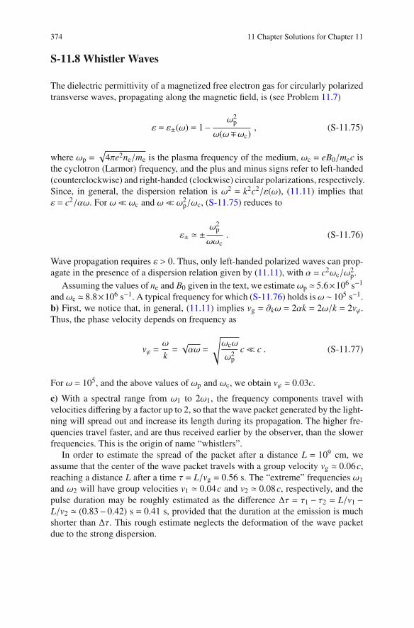
374 11 Chapter Solutions for Chapter 11
S-11.8 Whistler Waves
The dielectric permittivity of a magnetized free electron gas for circularly polarized
transverse waves, propagating along the magnetic field, is (see Problem 11.7)
ε = ε±(ω) = 1−ω2
p
ω(ω∓ωc), (S-11.75)
where ωp =√
4πe2ne/me is the plasma frequency of the medium, ωc = eB0/mec is
the cyclotron (Larmor) frequency, and the plus and minus signs refer to left-handed
(counterclockwise) and right-handed (clockwise) circular polarizations, respectively.
Since, in general, the dispersion relation is ω2 = k2c2/ε(ω), (11.11) implies that
ε = c2/αω. For ω≪ ωc and ω≪ ω2p/ωc, (S-11.75) reduces to
ε± ≃ ±ω2
p
ωωc. (S-11.76)
Wave propagation requires ε > 0. Thus, only left-handed polarized waves can prop-
agate in the presence of a dispersion relation given by (11.11), with α = c2ωc/ω2p.
Assuming the values of ne and B0 given in the text, we estimateωp ≃ 5.6×10⁶ s−1
andωc ≃ 8.8×10⁶ s−1. A typical frequency for which (S-11.76) holds isω∼ 105 s−1.
b) First, we notice that, in general, (11.11) implies vg = ∂kω = 2αk = 2ω/k = 2vϕ.
Thus, the phase velocity depends on frequency as
vϕ =ω
k=√αω =
√
ωcω
ω2p
c≪ c . (S-11.77)
For ω = 105, and the above values of ωp and ωc, we obtain vϕ ≃ 0.03c.
c) With a spectral range from ω1 to 2ω1, the frequency components travel with
velocities differing by a factor up to 2, so that the wave packet generated by the light-
ning will spread out and increase its length during its propagation. The higher fre-
quencies travel faster, and are thus received earlier by the observer, than the slower
frequencies. This is the origin of name “whistlers”.
In order to estimate the spread of the packet after a distance L = 109 cm, we
assume that the center of the wave packet travels with a group velocity vg ≃ 0.06c,
reaching a distance L after a time τ = L/vg = 0.56 s. The “extreme” frequencies ω1
and ω2 will have group velocities v1 ≃ 0.04c and v2 ≃ 0.08c, respectively, and the
pulse duration may be roughly estimated as the difference ∆τ = τ1 − τ2 = L/v1 −L/v2 ≃ (0.83− 0.42) s = 0.41 s, provided that the duration at the emission is much
shorter than ∆τ. This rough estimate neglects the deformation of the wave packet
due to the strong dispersion.

S-11.9 Wave Propagation in a “Pair” Plasma 375
S-11.9 Wave Propagation in a “Pair” Plasma
Actually, it is convenient to calculate the dispersion relation in the presence of an
external magnetic field B0 first, then, the answer to point a) is simply obtained as a
special case with B0 = 0. We assume B0 = B0 z and a wave linearly polarized along
x in a Cartesian reference frame xyz. The differential equations for the velocities of
positrons, v+, and electrons, v−, are respectively
dvx±dt= ± e
mec(Ex + vy±B0) ,
dvy±
dt= ∓ e
mec(vx±B0) , (S-11.78)
where we have assumed vz± = 0. Differentiating the first of (S-11.78) once more
with respect to t, and substituting the second of (S-11.78) for dvy±/dt, we obtain
d2vx±dt2
= ∓iωe
meEx ±
eB0
mec
dvy±
dt= ∓iω
e
meEx +ω
2cvx± , (S-11.79)
where ωc =√
eB0/mec is the cyclotron frequency. Substituting Ex = E0 e−iωt we
obtain
vx± = ∓iωe
me(ω2c −ω2)
E0 . (S-11.80)
Analogously, for vy± we have
vy± = ±eB0
mevx∓ = −iω
e
meE0 , (S-11.81)
which has the same value for both electrons and positrons. The components of the
current density are thus
Jx = n0 e (vx+− vx−) = − 2iωn0e2
me(ω2c −ω2)
E0 ,
Jy = n0 e (vy+− vy−) = 0 . (S-11.82)
The dielectric permittivity of the pair plasma, ε(ω), is obtained from the usual defi-
nitions J = σE = −iωχE and is
ε(ω) = 1−2ω2
p
ω2−ω2c
. (S-11.83)
The same result can be obtained for circular polarization, both for left-handed and
right-handed waves, confirming that there is no magnetically induced birefringence

376 11 Chapter Solutions for Chapter 11
in a pair plasma. This is different from the case of a medium containing free elec-
trons only, considered in Problem 11.7.
For case a), where B0 = 0, we set ωc = 0, and obtain a cut-off frequency at ω =
2ωp.
For case b), there is a resonance at ω = ωc, while wave propagation is forbidden
for frequencies in the range ωc < ω <
√
ω2c +2ω2
p.
S-11.10 Surface Waves
a) In a dielectric medium described by ε = ε(ω), a monochromatic EM field of
frequency ω satisfies the Helmoltz equation. Thus we have for the magnetic field
(
∇2+εω2
c2
)
Bz = 0 . (S-11.84)
Substituting (11.12) for Bz into the Helmholtz equation, we obtain
q2− k2+ω2
c2ε = 0 . (S-11.85)
b) From the equation c∇×B= 4πJ+∂tE and the definition of εwe obtain (for mono-
chromatic waves in complex notation) c∇×B = −iωεE. By substituting (11.12) for
B we obtain
− iωεE = (x∂y− y∂x)Bzc = (ikx−qy)Bzc , (S-11.86)
which gives for the electric field
E = −(kx+ iqy)c
εωBz . (S-11.87)
c) From the definition of S = cE×B/(4π) we find that S has components both along
x and along y, given by
S x =c
4πEyBz =
qcB20
4πεωe2qx cos(ky−ωt) sin(ky−ωt) , (S-11.88)
S y = −c
4πExBz =
kcB20
4πεωe2qx cos2(ky−ωt). (S-11.89)
However, averaging over one oscillation period we obtain 〈S x〉 = 0, thus the net
energy flux is in the y-direction only, since 〈S y〉 0.
d) The tangential component of the magnetic field at the interface between two
media must be continuous. Thus, from Bz(0−) = Bz(0
+) we get B1 = B2.

S-11.10 Surface Waves 377
e) Also the tangential component of the electric must be continuous at the interface,
thus Ey(0−) = Ey(0+). Using the results of points b) and d) we obtain
q1
ε1= −q2
ε2. (S-11.90)
Since both q1 > 0 and q2 > 0, ε1 and ε2 must have opposite signs.
f) Using the relationship (q1/ε1)2 = (q2/ε2)2 and the result of point a) we obtain
ε22
(
k2− ω2
c2ε1
)
= ε21
(
k2− ω2
c2ε2
)
, (S-11.91)
from which it follows that
ω2 = k2c2ε2
2−ε2
1
ε22ε1−ε21ε2
= k2c2 ε2+ε1
ε2ε1. (S-11.92)
Since wave can propagate only if k2 > 0, and ε1ε2 < 0, we get the additional condi-
tion ε1+ε2 < 0.
g) Since ε2 < −ε1 = −1 must hold, we may choose a metal, or a free electron gas, or
an ideal plasma . . . , for which ε2 = 1−ω2p/ω
2, and a frequency such thatω<ωp/√
2.
The above described EM modes are surface waves (also named surface plas-
mons). These waves propagate along the surface of a conductor and are evanescent
along the perpendicular direction, so that the EM energy is confined in a narrow
layer, thinner than the wavelength in vacuum. Surface waves are a building block
of plasmonics, a discipline oriented to develop optical and electronic devices on a
nanometric scale.1
S-11.11 Mie Resonance and a “Plasmonic Metamaterial”
a) The incident field can be written, in complex notation, as
Ei = Ei(x, t) = E0 eikx−iωt . (S-11.93)
Since a≪ λ, the electric field can be considered as uniform over the volume of the
sphere, thus Ei ≃ E0 e−iωt, assuming the center of the sphere to be located at x = 0.
1See e.g. W. L. Barnes et al., “Surface plasmon subwavelength optics”, Nature 424, 824 (2003); E.
Ozbay, “Plasmonics: merging photonics and electronics at nanoscale dimensions”, Science 311,
189 (2006).

378 11 Chapter Solutions for Chapter 11
Now we introduce a spherical coordinate system (r, θ,φ) with the origin at the center
of the sphere, and the zenith direction parallel to Ei. At the surface of the sphere,
r = a, we have the usual boundary conditions at the interface between two media
E⊥(a+, θ)−E⊥(a−, θ) = 4πσ(θ) , E‖(a+, θ)−E‖(a
−, θ) = 0 , (S-11.94)
where σ(θ) is the surface charge density on the sphere, independent of φ within our
approximations. The problem is thus analogous to the case of a dielectric sphere in
a static uniform external field, treated in Problem 3.4. We can extend the results for
the internal field and polarization to the case of an oscillating field as follows
Eint =3E0
εr(ω)+2, P = χEint =
3(εr(ω)−1)
4π(εr(ω)+2)E0 . (S-11.95)
The difference with the electrostatic case is that now εr depends on frequency, and
is not necessarily positive and greater than one, so that the internal field Eint can be
greater than the external applied field E0. A resonance appears when the real part of
the denominator vanishes. Setting η = 0 for simplicity, the resonance condition is
εr(ω)+2 = 3−ω2
p
ω2−ω20
= 0 , (S-11.96)
which yields
ω2 = ω20+ω2
p
3. (S-11.97)
The physical meaning of the resonance is particularly clear for ω0 = 0, e.g., for a
metallic (nano)sphere in a high-frequency (optical) field. In this case the resonance
frequency is
ω =ωp√
3, (S-11.98)
that is the natural frequency of the collective “Mie oscillations” of the electron
sphere treated in Problem 1.5, also known as the lowest-order surface plasmon of the
sphere. The resonance thus corresponds to the excitation of this oscillation mode.
b) The macroscopic polarization is given by the dipole moment of each nanosphere,
psphere = PV , with V = (4π/3)a3 the volume of the sphere, times the number of
nanospheres per unit volume, ns:
Pmacro = nspsphere = −3nsVω
2p
3ω2−ω2p
E0. (S-11.99)

S-11.11 Mie Resonance and a “Plasmonic Metamaterial” 379
This is equivalent to a macroscopic dielectric function
εr(ω) = 1−3nsVω
2p
3ω2−ω2p
. (S-11.100)
Wave propagation requires εr to be positive, i.e.,
ω <ωp√
3, ω >
ωp√3
√
1+3nsV . (S-11.101)
This is a simple example of an artificial “metamaterial”, where the plasmonic prop-
erties of the nanostructures composing the material determine the optical response.

Chapter S-12
Solutions for Chapter 12
S-12.1 The Coaxial Cable
a) Since the capacitance has been defined assuming static conditions and bound-
ary effects are negligible for an “infinite” wire, we evaluate the capacitance per unit
length of the cable, C, as for a cylindrical capacitor assuming the charge density to
be constant in time and uniformly distributed. For symmetry reasons the electrosta-
tic field between the two conductors is radial and independent of z and φ, and it is
obtained easily from Gauss’s law as
E =2λ
rr , a < r < b . (S-12.1)
Thus, the potential drop between the two conductors is
V = −∫ b
a
Er(r)dr = −2λ ln
(
b
a
)
, (S-12.2)
so that we obtain
C = λ|V | =1
2ln(b/a). (S-12.3)
∆z
b
a
z
Fig. S-12.1
Similarly, a static current I uniformly distrib-
uted on the inner conductor generates a mag-
netic field
B = Bφ(r) φ =2I
crφ . (S-12.4)
The inductance per unit length of the cable
can be obtained by evaluating the flux of B
c© Springer International Publishing AG 2017
A. Macchi et al., Problems in Classical Electromagnetism,
DOI 10.1007/978-3-319-63133-2 25
381

382 S-12 Solutions for Chapter 12
through a rectangle of width Δz, lying on a plane containing the z axis, and extending
from r = a to r = b, as highlighted in Fig. S-12.1. The flux is
Φ(B) =
∫ b
a
Bφ(r)Δzdr =2I
cln
(
b
a
)
Δz , (S-12.5)
corresponding to an inductance per unit length L
L = Φ(B)
IcΔz=
2
c2ln
(
b
a
)
. (S-12.6)
The same result can be obtained by calculating the magnetic energy in a cable
section of length Δz, and inductance ΔzL,
1
2ΔzL I2 ≡ Δz
∫ b
a
B2
8π2πr dr =
I2
c2ln
(
b
a
)
Δz . (S-12.7)
b) The coaxial cable is a continuous system with finite capacitance and inductance
per unit length, thus we know from Problem 7.4 that a current signal propagates
along the wire according to the wave equation (S-7.49), with velocity
v =1√LC= c . (S-12.8)
The general solution for the propagating current signal is thus I(z, t) = I(z− vt), and
propagation occurs with no dispersion. The associated charge signal λ(z, t) is related
to I(z, t) by the continuity equation,
∂tλ(z, t) = −∂zI(z, t) = −I′(z− ct) , (S-12.9)
where I′ denotes the derivative of I with respect to its argument. Since ∂tλ(z− ct) =
−cλ′(z− ct), we obtain
λ(z, t) = λ(z− ct) =1
cI(z− ct) . (S-12.10)
c) A transverse electric field E must be radial for symmetry reasons, E = Er(r,z, t) r.
Applying Gauss’s law to a cylindrical surface of radius a< r < b, infinitesimal height
Δz, and coaxial to the cable, we find Er = 2λ(z, t)/r. Again for symmetry reasons,
a transverse magnetic field must be azimuthal, B = Bφ(r,z, t) φ. Applying Stokes’
law to a circle of radius a < r < b, coaxial to the cable, we obtain Bφ = 2I(z, t)/rc.
The displacement current does not contribute to the flux through the circle, since
E is radial. Thus, the fields of have the same dependence on λ and I as the static
fields, the only difference being that here both λ = λ(z, t) and I = I(z, t) depend on
z and t. Notice that it is such peculiar character of the TEM configuration which

S-12.1 The Coaxial Cable 383
allows to use the capacitance and inductance calculated for static fields to obtain the
propagation velocity of electromagnetic signals along the cable, a result also true
for any transmission line in TEM mode.
We can check that the above fields constitute a solution to Maxwell’s equations
by verifying that
∇×E = ∂zEr φ =2
r∂zλ(z− ct) φ =
2
rλ′(z− ct) φ
=2
rcI′(z− ct) φ = − 2
rc2∂tI(z− ct) φ
= −1
c∂tB . (S-12.11)
d) The source at z = 0 must do a work W(t) in order to drive the current between the
inner and outer conductors,
W(t) = V(0, t) I(0, t) = −2cλ2(0, t) ln
(
b
a
)
. (S-12.12)
The local flux of energy at any point (r,φ,z), with a < r < b and z > 0, is
S(r,z, t) =c
4πE×B = z
c
4π
2λ(z− ct)
r
2I(z− ct)
rc
= zc
πr2λ2(z− ct) , (S-12.13)
corresponding to a total flow of energy at z
Φ(z, t) =
∫ b
a
S z 2πr dr = 2cλ2(z− ct) ln
(
b
a
)
= −W(z− ct) . (S-12.14)
This shows that the energy flow is sustained by the source.
e) The expressions for the fields, and for the capacitance and inductance per unit
length, are, in the presence of generic values of ε and μ,
Er = 2λ
εr, Bφ =
2μI
rc, (S-12.15)
C = ε
2ln(b/a), L = 2
c2ln
(
b
a
)
, (S-12.16)
corresponding to a wave velocity v = c/√εμ < c. In general, however, both ε and μ
can depend on frequency, and the cable becomes a dispersive transmission line with
phase velocity vφ(ω) = c/√
ε(ω)μ(ω).

384 S-12 Solutions for Chapter 12
S-12.2 Electric Power Transmission Line
a) The continuity equation is ∂tλ = −∂zI. Writing λ in the form λ = λ0 eikz−iωt, we
obtain
− iωλ0 = −ikI0 , or λ0 =k
ωI0 =
I0
vϕ, (S-12.17)
where vϕ is the phase velocity of the signal.
b) The electric field E can be calculated by applying Gauss’s law to a cylindrical
surface coaxial to the wire, obtaining
Er(r,z, t) =2λ(z, t)
r. (S-12.18)
The magnetic field B can be obtained from the equation c∇×B = 4πJ+∂tE. If we
choose a circle of radius r coaxial to the wire and apply Stokes’ theorem we have
∮
B ·dℓ = 1
c
∫
(4πJ+∂tE) ·dS . (S-12.19)
The ∂tE term is radial and thus does not contribute to the flux at the right-hand side,
so that
2πrBφ = 4πI
c, and Bφ(r,z, t) =
2I(z, t)
rc. (S-12.20)
The equations for Er(r,φ,z) and Bφ(r,φ,z) have the same form as in the static case of
a wire with constant and uniform charge density and current, respectively. We also
have |Er |/|Bφ| = c/vϕ. These are a typical properties of the TEM (transverse electro-
magnetic) mode for the transmission lines. Maxwell’s equation c∇×E = −∂tB gives
c∂zEr = −∂tBϕ leads to
ikλ0 = iωI0
c2⇒ k
I0
vϕ= ω
I0
c2⇒ ω
v2ϕ
=ω
c2⇒ vϕ = c , (S-12.21)
where we have used (S-12.17) and k = ω/vϕ.
In SI units we have
Er =λ
2πε0, Bφ =
μ0I
2πr,
|Er ||Bφ|=
c2
vϕ. (S-12.22)

S-12.2 Electric Power Transmission Line 385
d
+λ
E
−λ
h2θ
r
Fig. S-12.2
c) Consider a line on the midplane, at a distance h from
the plane containing the two wires, as in Figs. S-12.2
and S-12.3. The distance of the line from each wire is
r =√
h2+d2/4. The electric and magnetic fields gener-
ated by the two wires sum up to
E = 2x2I0
rcsinθe−iωt, (S-12.23)
B = 2y2I0
rcsinθe−iωt, (S-12.24)
with x and y the unit vectors parallel and perpendicular
to the plane containing the wires, respectively.
Since sinθ = d/(2r), we obtain
|Ex| = |By| =2I0 d
r2c. (S-12.25) d
h
B
+ I
2θ
− I
r
Fig. S-12.3
The corresponding expressions in SI units are
|Ex| = |By|c =I0 d
2πcε0r2=μ0I0 dc
2πr2. (S-12.26)
Thus
|By| =4π×10−7×103×5
2π× (302+52/22)T ≃ 10−6 T , (S-12.27)
and
|Ex| ≃ 3×10² V/m . (S-12.28)
For a comparison, the average magnetic field at the Earth surface is ∼ 5× 10⁻⁵ T,
while the electric field is ∼ 1.5×10² V/m. Possible screening effects by the Earth’s
surface have been neglected.
S-12.3 TEM and TM Modes in an “Open” Waveguide
a) Inserting (12.23) into the wave equation for B
(
∇2− 1
c2∂2
t
)
Bz = 0 , (S-12.29)

386 S-12 Solutions for Chapter 12
and recalling that ∂zBz = 0, we obtain the following relation between kx, ky and ω
k2x + k2
y −ω2
c2= 0 . (S-12.30)
b) The electric field of the wave can be obtained from
∂tE = c∇×B = c (x∂y− y∂x) Bz,
−iωE = cB0
[
−xky sin(kyy)− y ikx cos(kyy)]
eikx x−iωt , (S-12.31)
which leads to
Ex = −ikyc
ωB0 sin(kyy)eikx x−iωt , (S-12.32)
Ey =kxc
ωB0 cos(kyy)eikx x−iωt . (S-12.33)
c) The parallel component E‖ of the electric field E must vanish at the boundary with
a perfectly conducting surface, thus we must have Ex(y = ±a/2) = 0. This implies
that sin(kya/2) = 0, and kya = 2mπ, with m ∈ N. By substitution into (S-12.30) we
obtain
ω2 = k2xc2+
(
πc
a
)2
(2m)2 . (S-12.34)
The m = 0 mode corresponds to Ex = 0 and to Ey and Bz independent of y. The fields
are thus uniform over any cross-section of the waveguide parallel to the yz plane,
and we have ω= kxc. This is the TEM mode typical of transmission lines. The m= 1
mode has frequency
ω =
√
k2xc2+
(
2πc
a
)2
>2πc
a≡ ωco , (S-12.35)
where ωco ≡ 2πc/a is the cut-off frequency.
d) The energy flux is given by Poynting’s vector, parallel to the z = 0 plane,
S =c
4πE×B =
c
4π(EyBz x−ExBz y) . (S-12.36)
By averaging over one full cycle we find 〈S y〉 = 0, i.e., there is no net energy flux
along y. Averaging S x over one cycle we obtain
〈S x〉 =c2
8π
kx
ωB2
0 cos2(kyy) . (S-12.37)
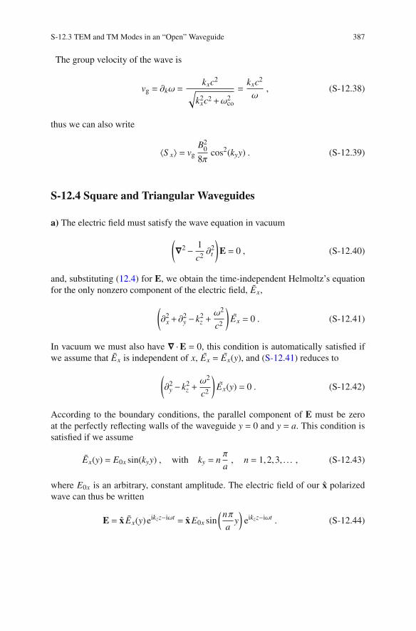
S-12.3 TEM and TM Modes in an “Open” Waveguide 387
The group velocity of the wave is
vg = ∂kω =kxc2
√
k2xc2+ω2
co
=kxc2
ω, (S-12.38)
thus we can also write
〈S x〉 = vg
B20
8πcos2(kyy) . (S-12.39)
S-12.4 Square and Triangular Waveguides
a) The electric field must satisfy the wave equation in vacuum
(
∇2− 1
c2∂2
t
)
E = 0 , (S-12.40)
and, substituting (12.4) for E, we obtain the time-independent Helmoltz’s equation
for the only nonzero component of the electric field, Ex,
(
∂2x +∂
2y − k2
z +ω2
c2
)
Ex = 0 . (S-12.41)
In vacuum we must also have ∇ ·E = 0, this condition is automatically satisfied if
we assume that Ex is independent of x, Ex = Ex(y), and (S-12.41) reduces to
(
∂2y − k2
z +ω2
c2
)
Ex(y) = 0 . (S-12.42)
According to the boundary conditions, the parallel component of E must be zero
at the perfectly reflecting walls of the waveguide y = 0 and y = a. This condition is
satisfied if we assume
Ex(y) = E0x sin(kyy) , with ky = nπ
a, n = 1,2,3, . . . , (S-12.43)
where E0x is an arbitrary, constant amplitude. The electric field of our x polarized
wave can thus be written
E = x Ex(y)eikzz−iωt = x E0x sin
(
nπ
ay
)
eikzz−iωt . (S-12.44)

388 S-12 Solutions for Chapter 12
Substituting (S-12.43) for Ex into (S-12.42) leads to
(
−k2y − k2
z +ω2
c2
)
E0x = 0 , (S-12.45)
which, diregarding the trivial case E0x = 0, is true only if
k2y + k2
z −ω2
c2= 0 , or kz =
√
ω2
c2− k2
y =
√
ω2
c2−n2π2
a2. (S-12.46)
The wave can propagate only if kz is real, thus we must have
ω > nπc
a. (S-12.47)
The cutoff frequency ωa is the lowest value of ω at which wave propagation occurs.
Since we must have n 1, we have ωa = πc/a. If we choose a frequency such that
πc/a < ω < 2πc/a, only the n = 1 mode can propagate in the guide.
The cross-section of the waveguide being square, the conditions for a y polarized
TE wave are obtained by interchanging the roles of x and y in all the above formulae,
and the electric field is
E = y E0y sin(kxx)eikzz−iωt = y E0y sin
(
mπ
ax
)
eikzz−iωt , (S-12.48)
with, again, E0y an arbitrary amplitude, m = 1,2,3, . . . , and the same dispersion rela-
tion as between ω and kz as above. Modes with m = n are degenerate, sharing the
same wavevector kz.
In general, a monochromatic TE wave propagating in the guide will be a super-
position of the two polarizations. The electric field will be
E =
[
x E0x sin
(
nπ
ay
)
+ y E0y sin
(
nπ
ax
)]
eikzz−iωt . (S-12.49)
b) In the case of the triangular waveguide, the parallel component of the electric
field E must be zero on the three x = 0, y = 0, and y = x planes. A field of the form
(S-12.49) already satisfies the boundary conditions at the x = 0 and y = 0 planes.
The additional condition at the y = x plane is E(x, x) · n = 0, where n = (−1,1,0)/√
2
is the unit vector perpendicular to the y = x plane. Thus
E ·h = E0x sin
(
nπ
ax
)
−E0y sin
(
nπ
ax
)
= 0 , (S-12.50)
which is satisfied if E0y = −E0x ≡ E0, so that we eventually obtain
E = E0
[
x sin
(
nπ
ay
)
− y sin
(
nπ
ax
)]
eikzz−iωt . (S-12.51)

S-12.5 Waveguide Modes as an Interference Effect 389
S-12.5 Waveguide Modes as an Interference Effect
xO p
y
p−1
p−2
p1
p2
+2a
+a
−a
+4a
−4a
−2a
A
Fig. S-12.4
a) The electrostatic potential φ must
be zero on the two conducting planes
at y = ±a, and the electric fields at
y = a− and y = −a+ must be perpen-
dicular to their surfaces (parallel to
y). The real dipole p is located at the
origin of our coordinate system, thus,
we need an image dipole equal to p,
located at (0,2a,0) and represented by
p1 in Fig. S-12.4, in order to fulfill
these conditions at the generic point A
of the y = +a plane. Analogously, the
real dipole p requires a further image
dipole p located at (0,−2a,0), repre-
sented by p−1 in Fig. S-12.4, in order
to fulfill the conditions at the y = −a
conducting plane. But now the three
dipoles p, p1, and p−1 together do not
generate a potential equal to zero on either plane. We can readjust the potential at
y = +a by adding a new image dipole equal to p, symmetrical to p−1, at (0,4a,0),
represented by p2. But this requires adding a further image dipole p−2, and so on.
Thus, the exact solution requires two infinite sets of equal image dipoles, pn and p−n,
with n = 1,2,3, . . . , located respectively at (0,2na,0) and (0,−2na,0). The resulting
electrostatic potential between the plates is finite because, for high n values, the
contribution of ±nth dipole is proportional to (2na)−2.
b) In order to fulfill the boundary conditions, all the image dipoles must oscillate
in phase with the real dipole. Consider the radiation emitted by each dipole in the
n ≡ (sinθ,cosθ,0) direction in the z = 0 plane, with wavevector k = (ω/c) n. In the
following we consider wavevectors lying in the z = 0 plane, but our considerations
apply to wavevectors lying in any plane containing the y axis, due to the rotational
symmetry of the problem. The optical path difference between the waves emitted by
two neighboring dipoles (real or images) is Δℓ = 2acosθ, as shown in Fig. S-12.5 for
the case of the real dipole p and the image p1. This corresponds to a phase difference
Δϕ = kΔℓ, and the condition for constructive interference is
kΔℓ =2ωa
ccosθ = 2πm, θ = arccos
(
mπc
ωa
)
, (S-12.52)

390 S-12 Solutions for Chapter 12
xO p
y
p−1
p−2
+2a
+a
−a
+4a
−4a
−2a
p2
p1
θ
∆
n
k
Fig. S-12.5
with m = 0,1,2, . . . . Due to the mirror symmetry of
the system for reflections through the y = 0 plane
(actually, antisymmetry, since all dipoles are inverted
by the reflection), if an angle θ satisfies (S-12.52)
for constructive interference, so does π− θ. In other
words, at large distance from the oscillating dipole,
each interference order m > 0 corresponds to the
superposition of two waves with wavevectors k± ≡(sinθ,±cosθ,0)ω/c, respectively.
The m = 0 condition corresponds to θ = π/2, and
the waves travels along the x axis. For m > 0, we can
write
kx =ω
csinθ =
ω
c
√
1− cos2 θ =ω
c
√
1−(
mπc
ωa
)2
=
√
ω2
c2−(
mπ
a
)2
, (S-12.53)
and kx is real only if ω > mπc/a. Thus, given a frequency ω, we observe only the
modes with m < ωa/(πc). If ω < πc/a, corresponding to a wavelength λ > 2a, only
the mode m = 0 can propagate.
c) Both magnetic fields must satisfy the wave equation
(c2∇2−∂2t )Bi = (c2∂2
x + c2∂2y −∂2
t )Bi = 0 , i = 0,1 , (S-12.54)
from which we obtain, denoting by k0 and k1 the respective wavevectors,
k20x c2 = ω2 , k2
1x c2+ k21y c2 = ω2 . (S-12.55)
d) Assuming electric fields of the form E = Ee−iωt, where E depends on the space
coordinates only, Maxwell’s equation in vacuum, ∂tE = c∇×B, gives
− iωE = c(x∂yBz− y∂xBz) . (S-12.56)
For the wave of type “0” we obtain
E0 = yk0xc
ωB0 eik0x x−iωt = y B0 eik0x x−iωt . (S-12.57)
For the wave of type “1” we obtain
E1 =ic
ωB1
[
yk1x cos(k1yy)− x ik1y sin(k1yy)]
eik1x x−iωt . (S-12.58)

S-12.5 Waveguide Modes as an Interference Effect 391
e) The “type-0” wave has the three vectors E0, B and k perpendicular to one another,
analogously to a plane wave in the free space (TEM mode). Further, E0 is perpen-
dicular to the two conducting surfaces, automatically satisfying the boundary con-
ditions. Thus, the frequency ω and the wavevector k = xk0x, with k0x = ω/c, are
subject to no constraint.
On the other hand, the electric field of the “type-1” wave has a component Ex
parallel to the two conducting surfaces, in addition to the transverse Ey component
(the mode is TM rather than TEM). The boundary conditions at y = ±a require that
Ex(y=±a)= 0. Thus we must have sin(±kya)= 0, or ky =mπ/a, with m= 1,2,3, . . . ,
leading to
kx =
√
ω2
c2−(
mπ
a
)2
. (S-12.59)
The m-th mode can propagate only if the corresponding kx is real, and has a lower
cut-off frequency ωco(m) = 2πmc/a-
A comparison to point (b) shows that the type-0 wave (TEM mode) corresponds
to the m = 0 interference order, while the type-1 waves (TM modes) correspond to
the > 0 interference orders. Actually, more precisely, we need not single dipoles,
but “dipole layers”, spread parallel to the z axis, in order to generate waves with
fields independent of z. If the real dipole of points (a) and (b) is parallel, rather than
perpendicular, to the conducting planes, the different boundary conditions would
lead to TE, rather than TM modes [1].
S-12.6 Propagation in an Optical Fiber
a) The electric field (12.6) corresponds to the sum of two plane waves of the same
frequency and different wavevectors, k1 and k2, propagating in the medium. For
both waves the dispersion relation is ω = kc/n, where n = n(ω) is the refractive
index of the medium. Both waves impinge on the medium-vacuum interface at the
angle θ, and the condition for total reflection is, according to Snell’s law,
sinθ >1
n
. (S-12.60)
b) The internal reflections at the y = ±a/2 planes turn the wave of type “1” into a
wave of type “2”, and vice versa. Thus the field amplitudes of the two waves at the
interface are related by the amplitude reflection coefficient r
E2(x,y = +a/2, t) = rE1(x,y = +a/2, t) ,
E1(x,y = −a/2, t) = rE2(x,y = −a/2, t) . (S-12.61)

392 S-12 Solutions for Chapter 12
For total reflection there is no transmission of energy through the y = ±a/2 planes,
thus the amplitudes of the incident and the reflected fields must be equal but for a
change of phase. For S -polarization (E parallel to the interface, as in our case) r is
written, according to the Fresnel equations,
r =ncosθ− i
√
n2 sin2 θ−1
ncosθ+ i√
n2 sin2 θ−1
, (S-12.62)
and, if nsinθ > 1, the square roots are real and |r| = 1. Thus we can write
r = eiδ = cosδ+ i sinδ , tanδ
2= −√
n2 sin2 θ−1
ncosθ. (S-12.63)
Substituting r= eiδ into (S-12.61) we obtain the following conditions at the y=±a/2
planes
E2 e−ikya/2 = E1 e+ikya/2 eiδ , E1 e−ikya/2 = E2 e+ikya/2 eiδ . (S-12.64)
By calculating the determinant of the homogeneous system for E1 and E2 we obtain
the condition
1 = e2i(kya+δ) , (S-12.65)
true if
2kya+2δ = 2mπ , m = 0,1,2, . . . . (S-12.66)
The implicit relation determining the allowed frequencies is
k2x =ω2
c2n
2− k2y > 0 . (S-12.67)
If nsinθ≫ 1 then δ ≃ −2θ, and if θ→ π/2 then
ky→ (m+1)π
a. (S-12.68)
c) All the above results are valid also for P-polarization, where the electric field of
the wave lies in the xy plane. Only (S-12.62) must be replaced by
r‖ = eiδ‖ =−n
2 cosθ+ i√
sin2 θ−n2
n2 cosθ+ i
√
sin2 θ−n2, (S-12.69)
corresponding to a different dependence of r and δ on θ.

S-12.7 Wave Propagation in a Filled Waveguide 393
S-12.7 Wave Propagation in a Filled Waveguide
a) The electric field E of a monochromatic EM wave of frequency ω propagating in
a medium of refractive index n = n(ω) satisfies Helmholtz’s equation
(
∇2+n2(ω)
ω2
c2
)
E = 0 . (S-12.70)
We are considering a TE mode with E = z Ez(y)eikx−iωt, thus we have
(
∂2y − k2+n
2(ω)ω2
c2
)
Ez(y) = 0 , (S-12.71)
whose general solution has the form s Ez(y) = Acos(qy)+ Bsin(qy), with A and B
two arbitrary constants. The electric field being parallel to the conducting walls at
y = ±a/2, the boundary conditions are Ez(y = ±a/2) = 0, from which we obtain
Ez(y) = E0
cos(qny) , n = 1,3,5 . . .
sin(qny) , n = 2,4,6 . . ., qn = n
π
a, (S-12.72)
and (S-12.71) turns into
q2n+ k2−n
2(ω)ω2
c2= 0 . (S-12.73)
The wave can propagate only if k is real, i.e., if ω > qnc ≡ ωn.
In the case of a plasma
q2n+ k2−
ω2−ω2p
c2= 0 , (S-12.74)
and the cut-off frequencies are
ω′n =√
q2nc2+ω2
p . (S-12.75)
b) The incident wave must be in the n = 1 mode, and its electric field is
Ei = z E0 cos(q1y)eik1 x−iωt , (S-12.76)
where k1 =
√
ω2/c2−q21. The total electric field is the sum of the incident field Ei
and the reflected field Er for x < 0, while only the transmitted field Et is present in
the x > 0 region. The boundary conditions at x = 0 is (Eiz +Erz)|x=0 = Etz|x=0, thus
all the waves must have the same dependence on t and y. The total field must thus be

394 S-12 Solutions for Chapter 12
Ez =
(
E0 eik1 x +Er e−ik1 x)
cos(q1y)e−iωt , x < 0 ,
Et cos(q1y )eikt x−iωt , x > 0 ,(S-12.77)
where kt =
√
n(ω)ω2/c2−q21. The boundary condition on the electric field yields
E0+Er = Et . (S-12.78)
In addition, the magnetic field must be also continuous at x= 0. From ∂tB=−c∇×E
we obtain
Bx =iπc
ωa×(
E0 eik1 x +Er e−ik1 x)
sin(q1y)e−iωt , x < 0 ,
Et sin(q1y)eikt x−iωt , x > 0 ,(S-12.79)
By = −c
ω×
k(
E0 eik1 x −Er e−ik1 x)
cos(q1y)e−iωt , x < 0 ,
ktEt cos(q1y)eikt x−iωt , x > 0 ,(S-12.80)
We notice that the continuity of Bx is ensured by the condition E0 +Er = Et, while
the continuity of By yields
k1(E0−Er) = ktEt . (S-12.81)
Eventually, we obtain
Er =k1− kt
k1+ ktE0 , Et =
2k1
k1+ ktE0 , (S-12.82)
which are identical to Fresnel’s formulas for S -polarization. In fact, the field of the
incoming wave (S-12.76) can be written as
Ei = z E0 cos(q1y)eik1 x−iωt = zE0
2
(
eiq1y+ e−iq1y)
eik1 x−iωt
= zE0
2eik1 x+iq1y−iωt + z
E0
2eik1 x−iq1y−iωt , (S-12.83)
which is the superposition of two z-polarized plane waves of equal amplitude, and
wavevectors of equal magnitude, but opposite y component, k = xk1 ± yq1. Thus
both plane waves impinge on the vacuum-medium interface at the same incidence
angle |θ| = arctan(q1/k1).
S-12.8 Schumann Resonances
a) Substituting the electric field (12.9) into the periodic boundary conditions (12.8)
we obtain

S-12.8 Schumann Resonances 395
eikxL = 1 , eikyL = 1 , (S-12.84)
solved by
kx = m2π
L, ky = n
2π
L, m,n = 0,1,2, . . . (S-12.85)
where m and n are not allowed to be zero simultaneously, and L = 2πR⊕. Since the
wave equations gives us ω2 = k2c2, we have
ω2 =
(
c
R⊕
)2
(m2+n2) . (S-12.86)
The lowest frequency corresponds to m = 1,n = 0 or m = 0,n = 1, and its value is
νmin =ωmin
2π=ω10
2π=
c
2πR⊕≃ 7.5s−1 , (S-12.87)
corresponding to a wavelength λmax = 2πR⊕ ≃ 40000km, the length of a great circle
of the Earth. The experimentally observed value is νmin ≃ 8s−1.
b) An ohmic conductor can be considered as perfectly reflecting at a frequency ω
if its conductivity σ(ω), assumed to be real, fulfills the condition σ(ω)≫ ω/4πke,
where ke = 1 in Gaussian units, and ke = 1/(4πε0) in SI units. Heuristically, the con-
dition corresponds to the conduction current J being much larger than Maxwell’s
displacement current. Since ε0 = 8.854× 10⁻¹² SI units, and σ/ω ≈ 0.6s Ω−1m−1,
sea water can be considered as a perfect conductor in the frequency range of the
Schumann resonances. In Gaussian units, the low-frequency conductivity of sea
water is σ ≃ 4×10¹⁰ s−1.
A discussion of Schumann resonances based on a “realistic” spherical geome-
try can be found in Reference [2], Section 8.9 and Problem 8.7. Nevertheless, our
simplified approach reveals the essential point that the characteristic length L of the
system, which determines the maximum wavelength for a standing wave (λ ≈ L),
is the Earth’s circumference, rather than the height of the ionosphere above the the
Earth’s surface.
References
1. R.P. Feynman, R.B. Leighton, M. Sands, The Feynman Lectures on Physics, Addison-Wesley
Publishing Company, Reading, MA 2006. Volume II, Section 24–8
2. J.D. Jackson, Classical Electrodynamics, § 9.2 and 9.4, 3rd Ed., Wiley, New York, London,
Sidney (1998)

Chapter S-13
Solutions for Chapter 13
S-13.1 Electrically and Magnetically Polarized Cylinders
(a) Long cylinders. In the “magnetic case”, the parallel component of the auxiliary
field, H =B/[(μ0)μr] (here, and the following, the parentheses mean that μ0 appears
in SI units only, not in Gaussian units) is continuous at the lateral surface of the
cylinder. Thus the magnetic field inside the cylinder, Bi, is
Bi = μrB0 . (S-13.1)
The interface condition for the electric field is that the parallel component of E must
be continuous at the lateral surface, thus we have for the internal field
Ei = E0 . (S-13.2)
These results are consistent with the analogy between the equations for E in
electrostatics and H in magnetostatics and in the absence of free currents, i.e., ∇×E = 0 and ∇×H = 0.
(b) Flat cylinders. In the “magnetic case”, the perpendicular component of B is
continuous at the bases, thus we have
Bi = B0 . (S-13.3)
In the “electric case”, the perpendicular component of the auxiliary vector D must
be continuous at the interface, thus internal field is
Ei =1
εrE0 . (S-13.4)
These results are consistent with the analogy between the equations for B and for
D in electrostatics and in the absence of free charges, i.e., ∇ ·B = 0 and ∇ ·D = 0.
c© Springer International Publishing AG 2017
A. Macchi et al., Problems in Classical Electromagnetism,
DOI 10.1007/978-3-319-63133-2 26
397
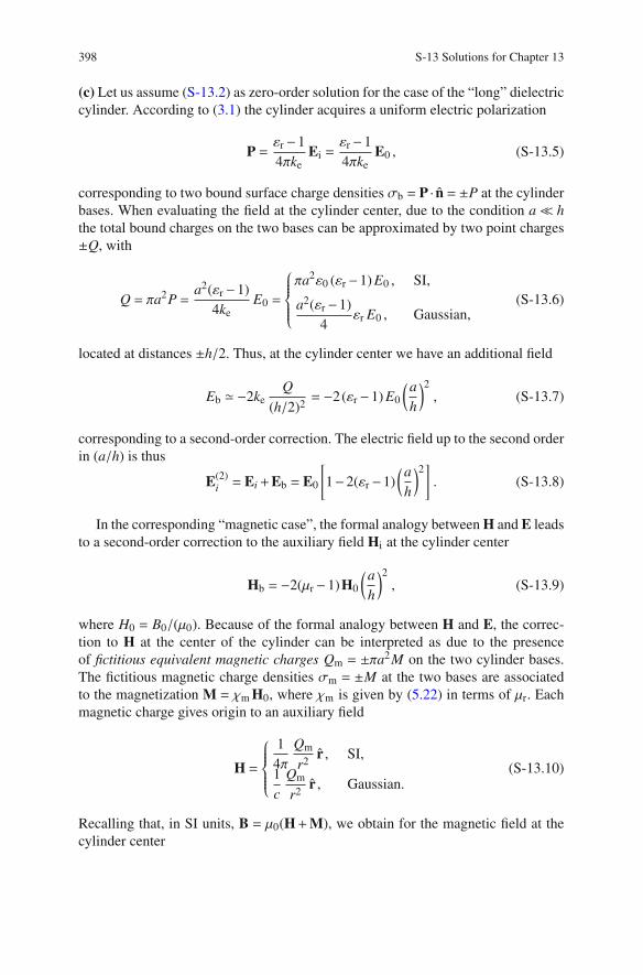
398 S-13 Solutions for Chapter 13
(c) Let us assume (S-13.2) as zero-order solution for the case of the “long” dielectric
cylinder. According to (3.1) the cylinder acquires a uniform electric polarization
P =εr−1
4πkeEi =
εr −1
4πkeE0 , (S-13.5)
corresponding to two bound surface charge densities σb = P · n = ±P at the cylinder
bases. When evaluating the field at the cylinder center, due to the condition a≪ h
the total bound charges on the two bases can be approximated by two point charges
±Q, with
Q = πa2P =a2(εr−1)
4keE0 =
⎧
⎪
⎪
⎪
⎪
⎨
⎪
⎪
⎪
⎪
⎩
πa2ε0 (εr−1) E0 , SI,
a2(εr−1)
4εr E0 , Gaussian,
(S-13.6)
located at distances ±h/2. Thus, at the cylinder center we have an additional field
Eb ≃ −2keQ
(h/2)2= −2(εr−1) E0
(
a
h
)2
, (S-13.7)
corresponding to a second-order correction. The electric field up to the second order
in (a/h) is thus
E(2)
i= Ei+Eb = E0
[
1−2(εr −1)
(
a
h
)2]
. (S-13.8)
In the corresponding “magnetic case”, the formal analogy between H and E leads
to a second-order correction to the auxiliary field Hi at the cylinder center
Hb = −2(μr−1)H0
(
a
h
)2
, (S-13.9)
where H0 = B0/(μ0). Because of the formal analogy between H and E, the correc-
tion to H at the center of the cylinder can be interpreted as due to the presence
of fictitious equivalent magnetic charges Qm = ±πa2M on the two cylinder bases.
The fictitious magnetic charge densities σm = ±M at the two bases are associated
to the magnetization M = χm H0, where χm is given by (5.22) in terms of μr. Each
magnetic charge gives origin to an auxiliary field
H =
⎧
⎪
⎪
⎪
⎪
⎨
⎪
⎪
⎪
⎪
⎩
1
4π
Qm
r2r , SI,
1
c
Qm
r2r , Gaussian.
(S-13.10)
Recalling that, in SI units, B = μ0(H+M), we obtain for the magnetic field at the
cylinder center

S-13.1 Electrically and Magnetically Polarized Cylinders 399
B = μ0(H0+M)+μ0Hb = μrH0+μ0Hb ≡ Bi+Bb , (S-13.11)
and the second-order correction is
Bb = −2(μr−1)B0
(
a
h
)2
. (S-13.12)
In Gaussian units we have B =H+4πM, the second order correction remaining the
same as in (S-13.12).
Notice that it would have been wrong to write
Bb = (μ0)μrHb (wrong!) , (S-13.13)
as it would have been wrong to write
Eb ≃ −2ke
εr
Q
(h/2)2= −2
(εr −1)
εrE0
(
a
h
)2
(wrong!) , (S-13.14)
instead of (S-13.7), because we are considering the fields generated by polariza-
tion charges, and inserting μr or εr would mean taking the effects of the medium
polarization into account twice.
Fig. S-13.1
Alternatively, we can recall that the zero-order
approximation of the cylinder magnetization is
M = χmHi = χmBi
(μ0)μr= χm
B0
(μ0), (S-13.15)
again, μ0 appearing in SI units only. The magnetiza-
tion is associated to a surface magnetization current
density Km =M× n/bm on the lateral surface of the
cylinder
Km =χm
bm
B0
(μ0)φ , (S-13.16)
where φ is the azimuthal unit vector of the cylindri-
cal coordinates with the cylinder axis as longitudi-
nal axis. Thus, the cylinder is equivalent to a finite
solenoid of height h and radius a, with the product
nI equal to a Km. The magnetic field of a finite solenoid on its axis is
BM = 2πkmnI (cosα1− cosα2) = 2πkmKm (cosα1− cosα2)
= 2πkmχm
bm
B0
(μ0)(cosα1− cosα2) = (μr−1)
B0
2(cosα1− cosα2) , (S-13.17)

400 S-13 Solutions for Chapter 13
where the angles α1 and α2 are shown in Fig. S-13.1. At the solenoid center we have
cosα1 = −cosα2 =h/2
√
a2+ (h/2)2≃ 1− 1
2
(
2a
h
)2
= 1−2
(
a
h
)2
, (S-13.18)
thus
BM ≃ (μr−1) B0
[
1−2
(
a
h
)2]
. (S-13.19)
The total field at the cylinder center equals the external field B0 plus the field due to
the cylinder magnetization
B(0) = B0+BM = μrB0−2μrB0
(
a
h
)2
+2B0
(
a
h
)2
= μrB0−2(μr−1)B0
(
a
h
)2
, (S-13.20)
in agreement with (S-13.19).
The correction to the field at the center of the magnetic “flat” cylinder can be
evaluated as due to a circular loop of radius a carrying an electric current Is = Kmh:
Bb =2πkmIs
a= 2πkmKm
h
a= 2π
km
bmM
h
a. (S-13.21)
At zeroth order we have
Hi ≃B0
(μ0)μr, thus M ≃ χm
B0
(μ0)μr, (S-13.22)
and we get
Bb =μr−1
2μr
a
hB0 . (S-13.23)
The auxiliary field H is given by (5.19), thus we have, up to the second order
Hi+Hb =B0+Bb
(μ0)μr=
⎧
⎪
⎪
⎪
⎪
⎨
⎪
⎪
⎪
⎪
⎩
B0+Bb
μ0−M = Hi+
Bb
μ0SI,
B0+Bb−4πM = Hi+Bb Gaussian.
(S-13.24)
Thus we have
Hb =Bb
(μ0)=μr−1
2μr
a
hH0 . (S-13.25)
Due to the formal analogy between H and E we have for the flat dielectric cylinder
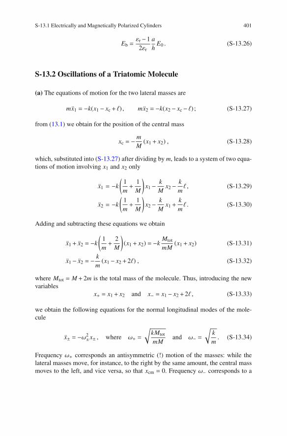
S-13.1 Electrically and Magnetically Polarized Cylinders 401
Eb =εr−1
2εr
a
hE0 . (S-13.26)
S-13.2 Oscillations of a Triatomic Molecule
(a) The equations of motion for the two lateral masses are
mx1 = −k(x1− xc+ ℓ) , mx2 = −k(x2− xc− ℓ) ; (S-13.27)
from (13.1) we obtain for the position of the central mass
xc = −m
M(x1+ x2) , (S-13.28)
which, substituted into (S-13.27) after dividing by m, leads to a system of two equa-
tions of motion involving x1 and x2 only
x1 = −k
(
1
m+
1
M
)
x1−k
Mx2−
k
mℓ , (S-13.29)
x2 = −k
(
1
m+
1
M
)
x2−k
Mx1+
k
mℓ . (S-13.30)
Adding and subtracting these equations we obtain
x1+ x2 = −k
(
1
m+
2
M
)
(x1+ x2) = −kMtot
mM(x1+ x2) (S-13.31)
x1− x2 = −k
m(x1− x2+2ℓ) , (S-13.32)
where Mtot = M + 2m is the total mass of the molecule. Thus, introducing the new
variables
x+ = x1+ x2 and x− = x1− x2+2ℓ , (S-13.33)
we obtain the following equations for the normal longitudinal modes of the mole-
cule
x± = −ω2±x± , where ω+ =
√
kMtot
mMand ω− =
√
k
m. (S-13.34)
Frequency ω+ corresponds an antisymmetric (!) motion of the masses: while the
lateral masses move, for instance, to the right by the same amount, the central mass
moves to the left, and vice versa, so that xcm = 0. Frequency ω− corresponds to a

402 S-13 Solutions for Chapter 13
symmetric motion: the lateral masses perform opposite oscillations, while the cen-
tral mass does not move.
(b) The electric dipole moment of the molecule is parallel to the molecular axis and
its magnitude is
p = −qx1+2qxc −qx2 = −q
(
1+2m
M
)
(x1+ x2) = −qMtot
Mx+ .
(S-13.35)
Thus, the dipole oscillates in the antisymetric mode at frequency ω+. The dipole
moment is zero when the molecule oscillates in the symmetric mode, and radiation
at frequency ω− is due only to quadrupole emission, which is weaker than dipole
emission.
(c) The initial conditions for x+ are
x+(0) = x1(0)+ x2(0) = d1+d2, x+(0) = 0 , (S-13.36)
thus for t > 0
x+(t) = (d1+d2)cosω+t . (S-13.37)
The symmetric mode is also excited, but does not contribute to the dipole radiation.
The instantaneous radiated power is
P =2
3c3| p|2 = 2q2
3c3
(
Mtot
M
)2
ω2+ (d1+d2)2 cos2ω+t . (S-13.38)
S-13.3 Impedance of an Infinite Ladder Network
Z2
Z1
Z0 = Z0
Fig. S-13.2
(a) Our infinite network is a sequence of
identical sections. As we did for Problem
4.10, we note that adding a further L-section
to the left of of Fig. 13.3 does not change the
impedance of the ladder network. Thus we
must have (see Fig. S-13.2).
Z0 = Z1+Z2Z0
Z2+Z0, (S-13.39)

S-13.3 Impedance of an Infinite Ladder Network 403
from which Z20−Z1Z0−Z1Z2 = 0 follows. The solution is
Z0 =Z1
2+
√
Z21
4+Z1Z2 , (S-13.40)
VNI0 I1
V1 V2IN−1
V0
Z1 Z1 Z1
Z2 Z2 Z2 Z0
Fig. S-13.3
The other solution of the quadratic
equation has been discarded
because in the case of real, posi-
tive impedances (the purely resis-
tive case of Problem 4.10) it would
give an unphysical negative value.
Thus, a finite ladder of N sections,
terminated by an impedance Z0 as
shown in Fig. S-13.3, is equivalent
to the infinite ladder.
(b) In Fig. 13.3, current In flows through the Z1 impedance of the (n+1)-th section,
thus, the voltage drop across the impedance, Vn −Vn+1, must equal InZ1. On the
other hand, In is input into the semi-infinite ladder network starting at node n, thus
we must have In = Vn/Z0. The two conditions give
Vn−Vn+1 =Vn
Z0Z1 , (S-13.41)
so that we obtain for the ratio of the voltages at adjacent nodes
α ≡ Vn+1
Vn
= 1− Z1
Z0. (S-13.42)
If V0(t) = V0 e−iωt is the input voltage, we have Vn = αnV0 e−iωt at the n-th node. For
a purely resistive network we have
Z0 ≡ R0 =R1
2+
√
R21
4+R1R2 , (S-13.43)
which is a real number, and α = 1−R1/R0 < 1. At each successive node the signal
is damped by a factor α.

404 S-13 Solutions for Chapter 13
(c) For the LC network we have
Z0 = −iωL
2+
√
−ω2L2
4+
iωL
iωC= − iωL
2+
√
L
C− ω
2L2
4
=
√
4L2
4LC− ω
2L2
4− iωL
2=
L
2
√
4
LC−ω2− iωL
2
=L
2
(√
ω2co−ω2− iω
)
, (S-13.44)
where ωco ≡ 2/√
LC. Thus
α = 1− Z1
Z0= 1+
2iωL
L
(
√
ω2co−ω2− iω
) =
√
ω2co−ω2+ iω
√
ω2co−ω2− iω
. (S-13.45)
If ω < ωco, the square roots are real and α is the ratio of a complex number to its
own complex conjugate, therefore |α| = 1, and we can write α = eiφ with
tan
(
φ
2
)
=ω
√
ω2co−ω2
. (S-13.46)
Thus the voltage at node n is Vn = V0 einφ−iωt, and the signal propagates along the
network without damping. The above equation also gives the dispersion relation
ω = ωco
∣
∣
∣
∣
∣
sin
(
φ
2
)
∣
∣
∣
∣
∣
. (S-13.47)
This is analogous to the dispersion relation (S-7.42) found in Problem 7.4, when we
substitute φ for ka.
If ω > ωco, Z0 is a purely imaginary number,
Z0 = ±i√
ω2−ωco , (S-13.48)
Fig. S-13.4
and α is real
α =±
√
ω2−ω2co+ω
±√
ω2−ω2co−ω
. (S-13.49)
Inserting the negative root into (S-13.49)
leads to |α| < 1, and the signal is damped. The

S-13.3 Impedance of an Infinite Ladder Network 405
positive root would lead to an unphysical |α| > 1, implying an amplification of the
signal along the network, without an external energy source.
Thus the LC network behaves as a low-pass filter, since signals at frequencies
ω>ωco are attenuated by a factor |α|N after N nodes. The dependence of the network
transmission on frequency approaches an ideal low-pass filter, for which transmis-
sion is zero for ω > ωco, at high numbers of circuit sections N. Figure S-13.4 shows
|α| (solid line) and |α|2 (dashed line) as a functions of the signal frequency ω.
(d) For the CL network (Problem 7.5) we proceed analogously to point (c) for the
LC network, and obtain
Z0 =i
2ωC+
√
− 1
4ω2C2+ωL
ωC=
1
2C
⎡
⎢
⎢
⎢
⎢
⎢
⎢
⎣
√
1
ω2co
− 1
ω2+
i
ω
⎤
⎥
⎥
⎥
⎥
⎥
⎥
⎦
, (S-13.50)
and
α =
√
ω−2co −ω−2− i/ω
√
ω−2co −ω−2+ i/ω
. (S-13.51)
We have undamped propagation for |α| = 1, i.e., when ω > ωco. For ω < ωco the
signals are damped, and the network acts as a high-pass filter.
S-13.4 Discharge of a Cylindrical Capacitor
(a) We use cylindrical coordinates (r,φ,z). For symmetry reasons, assuming h≫ b,
the electric field between the capacitor plates is radial, and easily evaluated from
Gauss’s law as
Er = Er(r) =2Q0
hr, (Gaussian units). (S-13.52)
The potential difference V across the plates is
V =
∣
∣
∣
∣
∣
∣
∫ b
a
E ·ds
∣
∣
∣
∣
∣
∣
=2Q0
h
∫ b
a
dr
r=
2Q0
hln(b/a) , (S-13.53)
and the capacity of our cylindrical capacitor is
C =Q0
V=
h
2ln(b/a)(S-13.54)

406 S-13 Solutions for Chapter 13
The initial electrostatic energy is Ues(0) = Q20/2C.
After the plates are connected through the resistor at t = 0, the system is an RC
circuit, and the capacitor charge at time t is
Q(t) = Q0 e−t/τ , where τ = RC =Rh
2ln(b/a)(S-13.55)
Assuming that the charge densities remain uniform over the plates during the dis-
charge, the absolute value of the charge of each plate between its bottom, z = 0, and
any height z < h (see Fig. S-13.5 for the case of the inner plate of Fig. 13.4) is
∆Q(z, t) = Q(t)z
h. (S-13.56)
The decay of the charge implies a current flowing over each plate, along the z direc-
tion. Let Ia(z, t) and Ib(z, t) be the currents in the inner and outer plate, respectively,
which can obtained from the continuity equation: for the inner plate
Ia(z, t) = −d[∆Q(z, t)]
dt=
Q(t)
τ
z
h=
Q0
τ
z
he−t/τ . (S-13.57)
a
r
R
O
z φ
h
z
∆Q
(z,t
)
I a(
)
I a(z
,t)
Fig. S-13.5
Since, in the assumption of uniform charge
densities, the charge on the outer plate is
−∆Q(z, t), then Ib(z, t) = −Ia(z, t).
We can evaluate B in the a < r < b region
from Maxwell’s equation
∇×B =4π
cJ+
1
c∂tE . (S-13.58)
The only nonzero component of J is along z
and the only nonzero component of E is along
r, given by
E = r2Q(t)
hr, (S-13.59)
while B must be independent of φ because of
the symmetry of our problem. Thus, according
to the curl components in cylindrical coordi-
nates of Table A.1 of the Appendix we have

S-13.4 Discharge of a Cylindrical Capacitor 407
(∇×B)r = −∂zBφ =1
c∂tEr ,
(∇×B)z =1
r∂r(rBφ) =
4π
cJz , (S-13.60)
and we see that the only nonzero component of B is Bφ, which can be evaluated
from either of (S-13.60). We choose the second of (S-13.60), and apply Stokes’
theorem to a circle C of radius a < r < b, coaxial to the capacitor and located at
height 0 < z < h,
∮
C
B(r,z, t) ·dℓ = 2πrBφ(r,z, t) =4π
cIa(z, t) , (S-13.61)
Bφ(r,z, t) =2
c
Ia(z, t)
r=
2
chτ
z
rQ0 e−t/τ . (S-13.62)
(b) The Poynting vector is
S =c
4πE×B = z
Q20
πh2τ
z
r2e−2t/τ , a < r < b , (S-13.63)
and S = 0 if r < a or r > b. The flux of S through a plane perpendicular to z at height
0 < z < h is thus
ΦS(z, t) =Q2
0z
πh2τe−2t/τ
∫ b
a
1
r22πr dr =
2Q20z ln(b/a)
h2τe−2t/τ . (S-13.64)
The electrostatic energy associated to the volume between the bottom of the capac-
itor (z = 0) and height z at time t is
∆Ues(z, t) =z
h
Q2(t)
2C=
z
h
Q20
e−2t/τ
2C=
z
h
Q20
ln(b/a)
he−2t/τ , (S-13.65)
because the electric field does not depend on z. Thus we have
d[∆Ues(z, t)]
dt= −2∆Ues(z, t)
τ= −ΦS(z, t) . (S-13.66)
(c) The assumptions of slowly varying currents and of uniform charge density are
closely related. In fact, the capacitor can be viewed as a portion of a coaxial cable
along which charge and current signals are propagating in TEM mode, at velocity c.
In these conditions, the charge density can be assumed as uniform if the propagation
of the signals is “instantaneous” with respect to the duration of the discharge, i.e., if
the propagation time h/c≪ τ. This is equivalent to assuming that the wavelengths
corresponding to the frequency spectrum of the signal are much larger than h, so
that the field can be considered as uniform along z.

408 S-13 Solutions for Chapter 13
We can reach the same conclusion by checking that the electric field E1, gener-
ated by the magnetic induction, is much smaller than the electrostatic field E0. From
Maxwell’s equation
∇×E1 ≃ −1
c∂tB , (S-13.67)
where the only nonzero component of B is Bφ, we obtain
∂zE1r =1
c
2
chτ2z
rQ0 e−t/τ
E1r =Q0
c2hτ2z2
re−t/τ =
1
2
(
z
cτ
)2
E0r . (S-13.68)
where E0r is from the second of (S-13.59). Thus E1r ≪ E0r if h≪ cτ.
S-13.5 Fields Generated by Spatially Periodic Surface Sources
(a) In this case fields and potential are electrostatic. The potential ϕ = ϕ(x,y) is a
solution of the 2D Laplace’s equation
(∂2x +∂
2y)ϕ = 0 for y 0, (S-13.69)
and, due to the symmetry of the source, must be an even function of y. We attempt to
find a solution by the method of separation of variables, i.e., we look for a solution
of the form ϕ = X(x)Y(y), where X depends only on x and Y only on y. Equation
(S-13.69) becomes
X′′(x)Y(y)+X(x)Y′′(y) = 0 , (S-13.70)
where the double primes denote the second derivatives. Dividing by X(x)Y(y) we
obtainY′′(y)
Y(y)= −X′′(x)
X(x), (S-13.71)
which must hold for every x,y, implying that both sides of the equation must equal
some constant value, which, for convenience, we denote by α2,
Y′′(y)
Y(y)= α2 ,
X′′(x)
X(x)= −α2 , (S-13.72)
whose solutions are
Y(y) = Ay e+αy+By e−αy , and X(x) = Ax e+iαx +Bx e−iαx , (S-13.73)

S-13.5 Fields Generated by Spatially Periodic Surface Sources 409
where Ax, Ay, Bx, and By are constants to be determined. Discarding the solutions
that diverge for |y| →∞, and fitting the x dependence to the dependence of σ, which
implies α = k, we obtain
ϕ = ϕ0 e−k|y| cos(kx) , (S-13.74)
where ϕ0 is a constant to be determined. The nonzero components of the electric
field are
Ex = −∂xϕ = kϕ0 e−k|y| sin(kx) ,
Ey = −∂yϕ = sgn(y)kϕ0 e−k|y| cos(kx) . (S-13.75)
The component Ex is continuous at the y = 0 plane, as expected, since ∇×E = 0. We
can obtain the relation between Ey at y = 0 and the surface charge density by using
Gauss’s law,
Ey(x,y = 0+)−Ey(x,y = 0−) = 4πσ(x) , (S-13.76)
from which we obtain the value of ϕ0, namely ϕ0 = 2πσ0/k, and, finally
ϕ =2πσ0
ke−k|y| cos(kx) . (S-13.77)
(b) Here we have magnetostatic fields. Due to the analogy between the Poisson
equations for the vector potential ∇2A = −4πJ/c, and for the scalar potential ∇2ϕ =
−4πρ, we can use (S-13.77) for obtaining the vector potential A as
A = z A0 e−k|y| cos(kx) , where A0 =2πK0
kc. (S-13.78)
The nonzero components of the magnetic field are
Bx = ∂yAz = −sgn(y)kA0 e−k|y| cos(kx) = −sgn(y)2πK0
ce−k|y| cos(kx) ,
By = −∂xAz = kA0 e−k|y| sin(kx) =2πK0
ce−k|y| sin(kx) . (S-13.79)
Thus, By is continuous at y = 0, as expected from ∇ ·B = 0. Further we have
Bx(x,y = 0+)−Bx(x,y = 0−) = −4π
cK0 cos(kx) , (S-13.80)
in agreement with Ampere’s law.
(c) Since σ = 0, also the scalar potential is zero, ϕ = 0. The inhomogeneous wave
equation for the vector potential A is, in the Lorentz gauge condition,
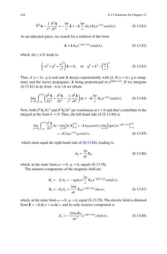
410 S-13 Solutions for Chapter 13
∇2A− 1
c2
∂2A
∂t2= −4π
cJ = −z
4π
cδ(y) K0 e−iωt cos(kx) . (S-13.81)
As an educated guess, we search for a solution of the form
A = z A0 e−q|y|−iωt cos(kx) , (S-13.82)
which, for y 0, leads to
(
−k2+q2+ω2
c2
)
A = 0 , or q2 = k2−(
ω
c
)2
. (S-13.83)
Thus, if ω < kc, q is real and A decays exponentially with |y|. If ω > kc, q is imag-
inary and the waves propagates, A being proportional to ei|q||y|−iωt. If we integrate
(S-13.81) in dy from −h to +h we obtain
limh→0
∫ +h
−h
(
∂2A
∂x2+∂2A
∂y2− 1
c2
∂2A
∂t2
)
dy = −z4π
cK0 e−iωt cos(kx) . (S-13.84)
Now, both ∂2A/∂x2 and ∂2A/∂t2 are continuous at y = 0 and don’t contribute to theintegral at the limit h→ 0. Thus, the left-hand side of (S-13.84) is
limh→0
∫ +h
−h
∂2A
∂y2dy = lim
h→0
[
∂yA]+h
−h= −z A0 qcos(kx) lim
h→0
[
sgn(y)e−q|y|−iωt]+h
−h
= −z2A0e−iωt qcos(kx) , (S-13.85)
which must equal the right-hand side of (S-13.84), leading to
A0 =2π
qcK0 (S-13.86)
which, at the static limit ω→ 0, q→ k, equals (S-13.78).
The nonzero components of the magnetic field are
Bx = ∂yAz = −sgn(y)2π
cK0 e−q|y|−iωt cos(kx) ,
By = −∂xAz =2πk
qcK0 e−q|y|−iωt sinωt , (S-13.87)
which, at the static limitω→ 0, q→ k, equal (S-13.79). The electric field is obtained
from E = −∂tA/c = iωA/c, and its only nonzero component is
Ez = −2πiωK0
qc2e−q|y|−iωt cos(kx) . (S-13.88)

S-13.5 Fields Generated by Spatially Periodic Surface Sources 411
(d) In this context, given a function f = f (x, t), we denote its time average by angle
brackets, and its space average by a bar, as follows
〈 f 〉 = ω2π
∫ +π/ω
−π/ωf dt , f =
k
2π
∫ +π/k
−π/kf dx . (S-13.89)
Thus we write the average power dissipated per unit time and unite surface on the
y = 0 plane as
⟨
KzEz
⟩
=1
2Re
[
K0
(
2πiω
qcK0
)∗]
cos2(kx) =πω
4c|K0|2 Re
(
−i
q
)
.
(S-13.90)
If q is real we have⟨
KzEz
⟩
= 0, consistently with the fields being evanescent for
|y| → ∞. There is no energy flow out of the y = 0 plane, and the work done by the
currents is zero on average. On the other hand, if q is imaginary, we have
⟨
KzEz
⟩
= −πω |K0|2
2|q|c , (S-13.91)
which equals minus the flux of electromagnetic energy out of the y = 0 plane. In
fact, the averaged Poynting vector is
⟨
S y
⟩
=c
4π
⟨
EzBx
⟩
=1
2
c
4πRe
[
2πiωK0
2qc
(
sgn(y)q∗2πK∗
0
q∗c
)]
cos2(kx)
= sgn(y)πω |K0|2
4|q|c , (S-13.92)
where we have used Re(i/q) = 1/|q| (for imaginary q). The flux of energy out of the
y = 0 plane is thus 2∣
∣
∣
∣
⟨
S y
⟩
∣
∣
∣
∣
= −⟨
KzEz
⟩
.
S-13.6 Energy and Momentum Flow Close to a Perfect Mirror
(a) The total electric field in front of the mirror is the sum of the fields of the incident
(Ei) and of the reflected (Er) waves, which have equal amplitude and frequency, but
opposite polarizations and wavevectors,

412 S-13 Solutions for Chapter 13
E = Ei+Er = y Eǫ [cos(kx−ωt)− cos(−kx−ωt)]
− zǫEǫ [sin(kx−ωt)− sin(−kx−ωt)]
= y Eǫ[cos(kx)cos(ωt)+ sin(kx) sin(ωt)− cos(kx)cos(ωt)+ sin(kxsin(ωt)]
− zǫEǫ[sin(kx)cos(ωt)− cos(kx) sin(ωt)+ sin(kx)cos(ωt)+ cos(kx) sin(ωt)]
= y2Eǫ sin(kx) sin(ωt)− z2ǫEǫ sin(kx)cos(ωt) , (S-13.93)
where Eǫ ≡ E0/√
1+ ǫ2. We can obtain the magnetic field from Maxwell’s equation
∂tB = −c∇×E = yc∂xEz− zc∂xEy
= −y2ǫEǫ ck cos(kx)cos(ωt)− z2Eǫ ck cos(kx) sin(ωt) , (S-13.94)
which yields, after integration in dt,
B = −y2ǫEǫck
ωcos(kx) sin(ωt)+ z2Eǫ
ck
ωcos(kx)cos(ωt)
= −y2ǫEǫ cos(kx) sin(ωt)+ z2Eǫ cos(kx)cos(ωt) , (S-13.95)
where we have used k = ω/c. The Poynting vector is
S =c
4πE×B = x
c
4π
(
EyBz−EzBy
)
= xcE2ǫ
π
[
sin(kx)cos(kx) sin(ωt)cos(ωt)− ǫ2 sin(kx)cos(kx)cos(ωt) sin(ωt)]
= xcE2ǫ
πsin(kx)cos(kx) sin(ωt)cos(ωt)
(
1− ǫ2)
= xc
4πE2ǫ
(
1− ǫ2)
sin(2kx) sin(2ωt) . (S-13.96)
Thus S = 0 if ǫ = 1, corresponding to circular polarization. In such a case, E is
parallel to B. In general, also when S 0, we have 〈S〉 = 0, and there is no net
energy flow.
(b) From the definition of Ti j we find
Fx = Txx =1
8πB2(0−) =
1
4πE2ǫ (cos2ωt+ ǫ2 sin2ωt)
=2I
c
[
1+1− ǫ2
1+ ǫ2cos2ωt
]
. (S-13.97)
The oscillating (at 2ω) component vanishes for circular polarization. The average
of Fx is the radiation pressure on the mirror (Problem 9.8), which does not depend
on polarization.

S-13.7 Laser Cooling of a Mirror 413
S-13.7 Laser Cooling of a Mirror
(a) A plane wave of intensity I exerts a radiation pressure 2I/c on a perfectly reflect-
ing surface. Thus the total force on the mirror, directed along the x axis of Fig. 13.5,
is
F =2A
c(I1− I2) . (S-13.98)
If I1 > I2 we have F > 0.
(b) The amplitudes of the electric fields of the two waves, in the mirror rest frame
S ′, are
E′1 = γ(E1−βB1) = γ(1−β) E1 =
√
1−β1+β
E1 , (S-13.99)
E′2 = γ(E2+βB2) = γ(1+β) E2 =
√
1+β
1−β E2 , (S-13.100)
where β= v/c, γ = 1/√
1−β2, and E1 = B1, E2 = B2 in Gaussian units. The intensity
of a plane wave is I = (c/4π) |E×B| = cE2/4π, thus we have
I′1 =1−β1+β
I1 , I′2 =1+β
1−β I2 . (S-13.101)
Since we have assumed I1 = I2, the total force is
F′ =2A
c(I′1− I′2) =
2A
c
(1−β)2− (1+β)2
1−β2= −8Aβγ2 I
c. (S-13.102)
(c) From the answer to point (b) we have F′ < 0, the direction of the force is opposite
to the direction of v. At the limit v≪ c, the force in the laboratory frame is equal to
the force in the mirror frame, and we have
F ≃ F′ ≃ −8AI
c2v , (S-13.103)
which is a viscous force. Under the action of this force, the mirror velocity will
decrease exponentially in time
v(t) = v(0)e−t/τ , where τ =Mc2
8AI. (S-13.104)
This effect has some analogies with the “laser-cooling” techniques, used in order
to cool atoms down to temperatures of the order of 10−6 K. These include, for

414 S-13 Solutions for Chapter 13
instance, Doppler cooling and Sisyphus cooling. The cooling of a macroscopic
mirror by radiation pressure has also been studied [1] for possible applications in
experiments of optical interferometry of ultra-high precision, e.g., for the detection
of gravitational waves.
S-13.8 Radiation Pressure on a Thin Foil
(a) It is instructive to solve this problem by three different methods. For definiteness
we assume a linearly polarized incident wave, with electric field Ei = y Ei eiki x−iωt,
where ki = ω/c; generalization to arbitrary polarization is straightforward.
First method (heuristic): we assume the incident plane wave to be a square pulse
of arbitrary but finite duration τ, and thus length cτ. The momentum of the wave
packet impinging on the surface A of the foil is, neglecting boundary effects,
pi =〈Si〉c2
cτA = x
⟨
|Ei|2⟩
4πcτA = x
E2i
8πcτA = x
I
cτA , (S-13.105)
where I = 〈|Si|〉 = c⟨
|Ei|2⟩
/(4π) = cE2i/(8π) is the intensity of the incident wave. The
reflected and transmitted wave packets have momenta
pr =〈Sr〉c2
cτA = −xRE2
i
8πcτA = −xR
I
cτA , (S-13.106)
pt =〈St〉c2
cτA = +xTE2
i
8πcτA = +xT
I
cτA , (S-13.107)
respectively, where R = |r|2, T = |t|2, and R+T = 1 because of energy conservation.
The amount of momentum transfered from the incident wave packet to the foil is
∆p = pi− (pr+pt) , (S-13.108)
resulting in a pressure pushing the foil toward positive x values (because ∆p > 0)
Prad =|∆p|τA=
[
1− (−R+T )] I
c= 2R
I
c. (S-13.109)
Second method: we calculate the average force on the foil, parallel to x, directly
as
〈F〉 =∫ d
0
〈J×B〉Adx , (S-13.110)

S-13.8 Radiation Pressure on a Thin Foil 415
where we have assumed the left surface of the foil located at x = 0, and the right
surface located at x = d. For a very small thickness d we can write
A
∫ d
0
〈J×B〉dx =1
2Ad
⟨
J(t)[
B(0+)+B(0−)]⟩
= −Ac
8π
⟨[
B2(0+)−B2(0−)]⟩
, (S-13.111)
where we have substituted J(t)=− [
B(0+)−B(0−)]
c/(4πd). Since we have |B(0+)|=|Et| = |t Ei|, and |B(0−)| =
∣
∣
∣Ei−Er
∣
∣
∣ =∣
∣
∣(1− r) Ei
∣
∣
∣, we can write the radiation pressure
on the foil as
Prad =〈|F|〉
A= −
E2i
16πc
(
|t|2− |1− r|2)
= − I
2c
(
|t|2− |1− r|2)
. (S-13.112)
Introducing the shorthand α = (ω2pd)/(2ωc) in (13.5), so that η = iα, we have
t =1
1+ iα, T = |t|2 = 1
1+α2, (S-13.113)
r = − iα
1+ iα, R = |r|2 = α2
1+α2, (S-13.114)
|1− r|2 = 1+5α2+4α4
(1+α2)2, |t|2− |1− r|2 = − 4α2
1+α2, (S-13.115)
and finally
Prad =I
2c2
4α2
1+α2= 2R
I
c. (S-13.116)
Third method: we calculate the flow of EM momentum directly using Maxwell’s
stress tensor Ti j. The theorem of EM momentum conservation states that
dpi
dt=
∮
S
Ti j n j dS (S-13.117)
(summation over the repeated index is implied), where n is the unit vector normal
to the surface S which envelops the thin foil, and p is the total momentum (EM and
mechanical) of the foil. Since in a steady state the EM contribution is constant, the
RHS of (S-13.117) equals the variation of mechanical momentum, i.e., the force.
Taking into account that the electric field has only the component Ey and the
magnetic field only the component Bz, and that n = ∓x on the left (x = 0−) and right
(x = 0+) surfaces, respectively, the only relevant component of Ti j is Txx, and
dpx
dt=
[
Txx(0+)−Txx(0−)]
A . (S-13.118)

416 S-13 Solutions for Chapter 13
For Txx(0+) and Txx(0−) we have
Txx(0+) = − 1
8π
⟨
E2(0+)+B2(0+)⟩
= − 1
4π
⟨
|Et|2(0+)⟩
= −TE2
i
8π,
Txx(0−) = − 1
8π
⟨
E2(0−)+B2(0−)⟩
= −
⟨
E2i
⟩
8π
[
|(1+ r)|2+ |(1− r)|2]
= −E2
i
16π
(
1+ |r|2+ rr∗+1+ |r|2− rr
∗)
= −(1+R)E2
i
8π. (S-13.119)
Thus
dpx
dt=
E2i
8π(−T +1+R) A = 2R
I
cA , (S-13.120)
which yields (13.6) again.
(b) From the Lorentz transformation of the fields we obtain the intensity of the
incident wave in the S ′ frame, where the foil is at rest,
I′ =1−β1+β
I , (S-13.121)
and the force on the foil in S ′ is F′ = 2AI′/c. Since for a force parallel to v we have
F = F′, in the laboratory frame S we can write
F = F′ = 21−β1+β
I
cA . (S-13.122)
(c) The radiation pressure must be multiplied by a factor R = R(ω′) in the frame S ′,where the frequency is ω′ =
√
(1−β)/(1+β)ω. Thus
F = 21−β1+β
R(
ω′) I
cA , ω′ =
√
1−β1+β
ω. (S-13.123)

S-13.9 Thomson Scattering in the Presence of a Magnetic Field 417
S-13.9 Thomson Scattering in the Presence of a Magnetic Field
(a) We write the fields in the complex notation. Within our assumptions, the equation
of motion for the electron is
medv
dt= −e
(
E+v
c×B0
)
, (S-13.124)
where −e and me are the charge and mass of the electron, respectively. The solution
has already been evaluated in Problem 7.10, and is
vx =ωc
ω2c −ω2
e
meEi e−iωt , vy =
iω
ω2c −ω2
e
meEi e−iωt , (S-13.125)
and vz = 0.
(b) The cycle-averaged radiated power is
〈P〉 = e4
3m2ec3|Ei|2
ω2
(
ω2c −ω2
)2
(
ω2c +ω
2)
, (S-13.126)
which is maximum at the cyclotron resonance, ω = ωc. At the low-frequency limit
ω/ωc ≪ 1 we have 〈P〉 ∝ ω2/ω2c , while at the high-frequency limit ω/ωc ≫ 1 the
power is independent of frequency (“white” spectrum).
The orbit of the electron is elliptical, consequently the angular distribution and
polarization of the scattered radiation are analogous to what found for an elec-
tron in the presence of an elliptically polarized wave, in the absence of external
magnetic fields, as discussed in Problem 10.9. According to (S-13.125) we have
vx/vy = −iωc/ω. At the limit ω ≪ ωc we have⟨
|vx|⟩
≫⟨
|vy|⟩
, the major axis of
the elliptical orbit of the electron is thus parallel to x, and the strongest radia-
tion intensity is observed on the yz plane. At the opposite limit, ω≫ ωc, we have⟨
|vx|⟩
≪⟨
|vy|⟩
, the major axis of the orbit is parallel to y, and the strongest radiation
intensity is observed on the xz plane.
S-13.10 Undulator Radiation
(a) According to Maxwell’s equation ∇ ·B = 0, we must have
∂xBx = −∂yBy = −(∂yb)cos(kx) , (S-13.127)
which, after integration in dx, leads to

418 S-13 Solutions for Chapter 13
Bx = −(∂yb)sin(kx)
k, (S-13.128)
where we have set to zero the integration constant. In static conditions, and in the
absence of electric currents, we have ∇×B = 0, thus we must also have
0 = ∂xBy−∂yBx = −kb(y) sin(kx)+ (∂2yb)
sin(kx)
k, (S-13.129)
which, divided by sin(kx), reduces to
∂2yb(y) = k2b(y) . (S-13.130)
The even solution (S-13.130) is
b(y) = B0 cosh(ky) , (S-13.131)
where B0 is a constant to be determined. Thus the two nonzero components of B
are
Bx = −B0 sin(kx) sinh(ky) , By = B0 cos(kx)cosh(ky) , (S-13.132)
and on the z axis, where x = 0 and y = 0, we have
B(0,0,z) = yB0 . (S-13.133)
(b) The Lorentz transformations from the laboratory frame S to S ′ give for the fields
in S ′
B′x = Bx[x(x′, t′),y′] = −B0 sinh(ky′) sin[kγ(x′+ vt′)] , (S-13.134)
B′y = γBy[x(x′, t′),y′] = γB0 cosh(ky′)cos[kγ(x′+ vt′)] , (S-13.135)
E′z = γvBy[x(x′, t′),y′] = γvB0 cosh(ky′)cos[kγ(x′+ vt′)].
(S-13.136)
where γ = 1/√
1− v2/c2. Since the boost is parallel to the x axis, we have y′ = y.
Disregarding the magnetic force in S ′, the electron oscillates along z′ under the
action of the electric field E′ = E′z(0,0, t′) = γvB0 cos(ω′t′), where ω′ = kγv. Thus,
in S ′, we observe a Thomson scattering, and the electron emits electric-dipole radi-
ation of frequency ω′.(d) Transforming back to S , the frequencies of the radiation emitted in the forward
(+) and backward (−) directions are
ω± = γ(1±β)ω′ = γ(1±β)kγv = kcγ2β(1±β) , (S-13.137)
where β = v/c.

S-13.10 Undulator Radiation 419
In S ′, the electron does not emit radiation along its direction of oscillation, i.e.,
along z′. This corresponds to two “forbidden” wavevectors k′ ≡ (0,0,ω′/c) and k′ ≡(0,0,−ω′/c). By a back transformation to S we obtain
kx = γ
(
k′x ±ω′
cβ
)
= ±γβ ω′
c, ky = 0 , kz = k′z =
ω′
c, (S-13.138)
thus, in S , we have no radiation emission at the angles ±θ in the xz plane such that
tanθ =kz
kx
=1
γβ. (S-13.139)
The “undulator radiation”, emitted by high-energy electrons injected along a peri-
odically modulated magnetic field, is at the basis of free-electron lasers emitting
coherent radiation in the X-ray frequency range.
S-13.11 Electromagnetic Torque on a Conducting Sphere
(a) We can write the electric field of the wave as
E(z, t) = E0[xcos(kz−ωt)− ysin(kz−ωt)]
= Re[E0(x+ iy)ei(kz−ωt)] , (S-13.140)
where k =ω/c= 2π/λ. Since a≪ λ, we can consider the electric and magnetic fields
of the wave as uniform over the volume of the sphere, and neglect the magnetic
induction effects. Thus, the sphere can be considered as located in a uniform rotating
electric field
E0(t) = Re(
E0 e−iωt)
, where E0 = E0(x+ iy) . (S-13.141)
In the presence of oscillating fields, the complex electric permittivity of a medium
of real conductivity σ is defined as
ε(ω) = 1+4πiσ
ω. (S-13.142)
Thus, our problem is analogous to Problem 3.4, where we considered a dielectric
sphere in a uniform external electric field. The internal electric field and the dipole
moment of the sphere are

420 S-13 Solutions for Chapter 13
Eint =3
ε+2E0 =
3E0
3+4πiσ/ω= − 3iωtd
1−3iωtdE0 , (S-13.143)
p = PV = χEintV =3V
4π
ε−1
ε+2E0 =
3V
4π
4πiσ/ω
3+4πiσ/ωE0 ,
=3V
4π
4πiσ
3ω+4πiσE0 =
3V
4π
i/td
3ω+ i/tdE0 =
3V
4π
i
3ωtd+ iE0
=3V
4π
1+3iωtd
(3ωtd)2+1E0 (S-13.144)
where V = 4πa3/3 is the volume of the sphere, and td = 1/(4πσ). By writing the
complex numerator in terms of its modulus and argument we have
1+3iωtd =
√
1+ (3ωtd)2 eiφ , where φ = arctan(3ωtd) , (S-13.145)
and, substituting into (S-13.144) we obtain
p =3V
4π
E0√
1+ (3ωtd)2eiφ , (S-13.146)
and, for the real quantity,
p = Re
⎡
⎢
⎢
⎢
⎢
⎢
⎣
3V
4π
E0√
1+ (3ωtd)2(x+ iy)e−i(ωt−φ)
⎤
⎥
⎥
⎥
⎥
⎥
⎦
=3V
4π
E0√
1+ (3ωtd)2[xcos(ωt−φ)+ ysin(ωt−φ)] . (S-13.147)
Thus the dipole moment of the sphere rotates with a phase delay φ relative to the
electric field of the wave.
(b) The torque acting on an electric dipole p in the presence of an electric field E is
τ = p×E. In our case, the angle between p and E0 is constant in time and equal to
φ, thus the torque is
τ = z |p||E0|sinφ = z3V
4π
E20
√
1+ (3ωtd)2sinφ. (S-13.148)
The same result can be obtained by evaluating
τ =1
2Re
(
p× E∗)= Re
⎡
⎢
⎢
⎢
⎢
⎢
⎣
3V
8π
E20
eiφ
√
1+ (3ωtd)2(x+ iy)× (x− iy)
⎤
⎥
⎥
⎥
⎥
⎥
⎦
= Re
⎡
⎢
⎢
⎢
⎢
⎢
⎣
3V
8π
E20
(cosφ+ i sinφ)√
1+ (3ωtd)2(−2i z)
⎤
⎥
⎥
⎥
⎥
⎥
⎦
= z3V
4π
E20
√
1+ (3ωtd)2sinφ. (S-13.149)

S-13.12 Surface Waves in a Thin Foil 421
S-13.12 Surface Waves in a Thin Foil
(a) As an educated guess, we search for solutions for the unknown quantities Ex,
and Bz of the form
Ex(x,y, t) = Ex(x)eiky−iωt , Bz(x,y, t) = Bz(x)eiky−iωt , (S-13.150)
where Ex(x), and Bz(x) are complex functions to be determined. According to
(13.10), Ey is symmetric (even) for reflection across the x = 0 plane. Since in vac-
uum we have ∇ ·E = ∂xEx +∂yEy = 0, we obtain
∂xEx = −ikE0 e−q|x| , (S-13.151)
which, after integration in dx, leads to
Ex(x) = sgn(x)ik
qE0 e−q|x| =
⎧
⎪
⎪
⎪
⎪
⎪
⎪
⎨
⎪
⎪
⎪
⎪
⎪
⎪
⎩
− ik
qE0 eqx , x < 0,
ik
qE0 e−qx , x > 0.
(S-13.152)
Thus, the Ex component is antisymmetric (odd) for reflection across the x = 0 plane.
Since our fields are independent of z, Maxwell’s equation ∇×E = −∂tB/c reduces
to
− 1
c∂tBz = ∂xEy−∂yEx = sgn(x)
(
k2
q−q
)
E0 e−q|x| ei(ky−ωt) , (S-13.153)
which, after integration in dt and division by −ei(ky−ωt)/c, leads to
Bz = sgn(x)ic
qω
(
q2− k2)
E0 e−q|x| , (S-13.154)
thus Bz, like Ex, is an odd function of x.
Fig. S-13.6
We can obtain the surface charge density σ(y, t)
and the surface current density K(y, t) on the foil
from the boundary conditions at the x = 0 plane.
Figure S-13.6 shows the surface current K and the
magnetic field close to the foil.
σ(y, t) =1
4π
[
Ex
(
x = 0+,y, t)−Ex
(
x = 0−,y, t)]
= i2k
qE0 ei(ky−ωt) , (S-13.155)
Ky(y, t) = − c
4π
[
Bz
(
x = 0+,y, t)−Bz
(
x = 0−,y, t)]

422 S-13 Solutions for Chapter 13
− ic2
2πqω
(
q2− k2)
E0 ei(ky−ωt) , (S-13.156)
while the z component of K is zero because its presence would imply a nonzero y
component of B.
(b) The time-averaged Poynting vector can be written as
〈S〉 = c
4π〈E×B〉 = c
8π
[
x Re(EyB∗z )− y Re(ExB∗z )]
, (S-13.157)
where
EyB∗z = −sgn(x)ic
qω
(
q2− k2)
|E0|2 e−2q|x|, (S-13.158)
ExB∗z =kc
q2ω
(
q2− k2)
|E0|2 e−2q|x| . (S-13.159)
We thus obtain 〈S x〉 = 0 because EyB∗z , is purely imaginary, and the energy flow is
in the y direction only:
〈S〉 = −ykc
8πq2ω
(
q2− k2)
|E0|2 e−2q|x| . (S-13.160)
(c) Form Helmholtz’s equation, we obtain
q2− k2+ω2
c2= 0 . (S-13.161)
(d) From (S-13.156) we can write, within our approximations,
J =K
ℓ= −y i
c2
2πqℓω
(
q2− k2)
E0 ei(ky−ωt) (S-13.162)
and, combining with (13.11), we obtain
−ic2
2πqℓω
(
q2− k2)
E0 ei(ky−ωt) = 4πiω2
p
ωE0 ei(ky−ωt) ,
q2− k2 = −8π2ω2
p
c2qℓ . (S-13.163)
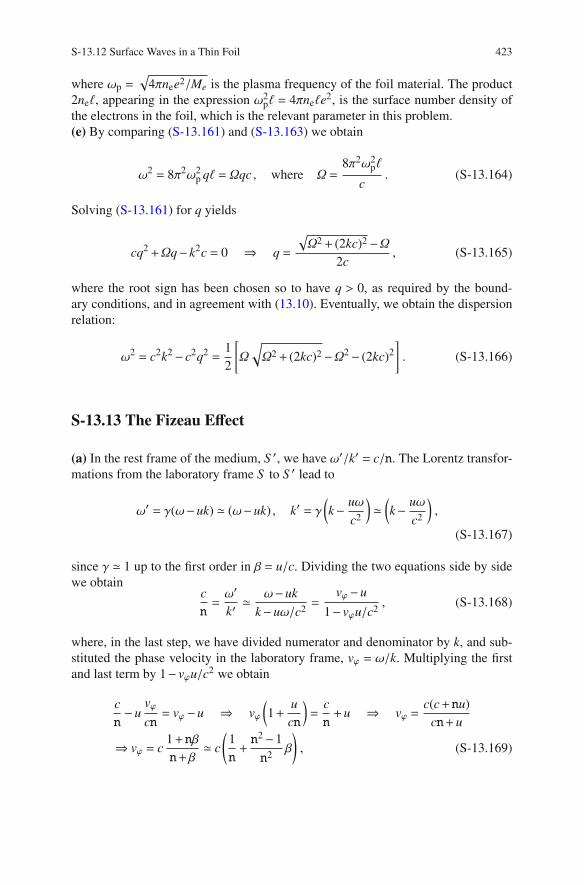
S-13.12 Surface Waves in a Thin Foil 423
where ωp =√
4πnee2/Me is the plasma frequency of the foil material. The product
2neℓ, appearing in the expression ω2pℓ = 4πneℓe
2, is the surface number density of
the electrons in the foil, which is the relevant parameter in this problem.
(e) By comparing (S-13.161) and (S-13.163) we obtain
ω2 = 8π2ω2p qℓ = Ωqc , where Ω =
8π2ω2pℓ
c. (S-13.164)
Solving (S-13.161) for q yields
cq2+Ωq− k2c = 0 ⇒ q =
√
Ω2+ (2kc)2−Ω2c
, (S-13.165)
where the root sign has been chosen so to have q > 0, as required by the bound-
ary conditions, and in agreement with (13.10). Eventually, we obtain the dispersion
relation:
ω2 = c2k2− c2q2 =1
2
[
Ω
√
Ω2+ (2kc)2−Ω2− (2kc)2
]
. (S-13.166)
S-13.13 The Fizeau Effect
(a) In the rest frame of the medium, S ′, we have ω′/k′ = c/n. The Lorentz transfor-
mations from the laboratory frame S to S ′ lead to
ω′ = γ(ω−uk) ≃ (ω−uk) , k′ = γ(
k− uω
c2
)
≃(
k− uω
c2
)
,
(S-13.167)
since γ ≃ 1 up to the first order in β = u/c. Dividing the two equations side by side
we obtainc
n=ω′
k′≃ ω−uk
k−uω/c2=
vϕ−u
1− vϕu/c2, (S-13.168)
where, in the last step, we have divided numerator and denominator by k, and sub-
stituted the phase velocity in the laboratory frame, vϕ = ω/k. Multiplying the first
and last term by 1− vϕu/c2 we obtain
c
n−u
vϕ
cn= vϕ−u ⇒ vϕ
(
1+u
cn
)
=c
n+u ⇒ vϕ =
c(c+nu)
cn+u
⇒ vϕ = c1+nβ
n+β≃ c
(
1
n+n2−1
n2β
)
, (S-13.169)
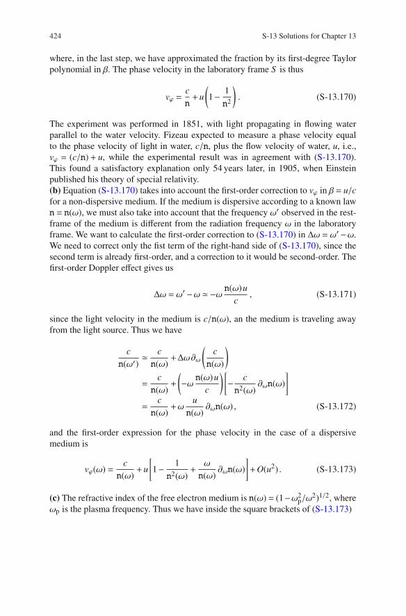
424 S-13 Solutions for Chapter 13
where, in the last step, we have approximated the fraction by its first-degree Taylor
polynomial in β. The phase velocity in the laboratory frame S is thus
vϕ =c
n+u
(
1− 1
n2
)
. (S-13.170)
The experiment was performed in 1851, with light propagating in flowing water
parallel to the water velocity. Fizeau expected to measure a phase velocity equal
to the phase velocity of light in water, c/n, plus the flow velocity of water, u, i.e.,
vϕ = (c/n) + u, while the experimental result was in agreement with (S-13.170).
This found a satisfactory explanation only 54 years later, in 1905, when Einstein
published his theory of special relativity.
(b) Equation (S-13.170) takes into account the first-order correction to vϕ in β = u/c
for a non-dispersive medium. If the medium is dispersive according to a known law
n = n(ω), we must also take into account that the frequency ω′ observed in the rest-
frame of the medium is different from the radiation frequency ω in the laboratory
frame. We want to calculate the first-order correction to (S-13.170) in ∆ω = ω′−ω.
We need to correct only the fist term of the right-hand side of (S-13.170), since the
second term is already first-order, and a correction to it would be second-order. The
first-order Doppler effect gives us
∆ω = ω′−ω ≃ −ω n(ω)u
c, (S-13.171)
since the light velocity in the medium is c/n(ω), an the medium is traveling away
from the light source. Thus we have
c
n(ω′)≃ c
n(ω)+∆ω∂ω
(
c
n(ω)
)
=c
n(ω)+
(
−ω n(ω)u
c
)[
− c
n2(ω)∂ωn(ω)
]
=c
n(ω)+ω
u
n(ω)∂ωn(ω) , (S-13.172)
and the first-order expression for the phase velocity in the case of a dispersive
medium is
vϕ(ω) =c
n(ω)+u
[
1− 1
n2(ω)+ω
n(ω)∂ωn(ω)
]
+O(u2) . (S-13.173)
(c) The refractive index of the free electron medium is n(ω) = (1−ω2p/ω
2)1/2, where
ωp is the plasma frequency. Thus we have inside the square brackets of (S-13.173)

S-13.13 The Fizeau Effect 425
1− 1
n2(ω)= − 1
1−ω2p/ω
2=ω2
p
ω2−ω2p
, (S-13.174)
and
ω
n(ω)∂ωn(ω) = − ω
(1−ω2p/ω
2)1/2
1
(1−ω2p/ω
2)3/2
ω2p
ω3= −
ω2p
ω2−ω2p
, (S-13.175)
so that the two first-order corrections to vϕ(ω) cancel out, and the phase velocity is
independent of the flow velocity of the medium up to the second order in β.
S-13.14 Lorentz Transformations for Longitudinal Waves
(a) The Lorentz transformations for the wave frequency and wavevector are, in the
case of a boost along x,
ω′L = γ (ωL −VkL) , k′L = γ(
kL−VωL
c2
)
, (S-13.176)
where γ = 1/√
1−V2/c2. In the special case where the boost velocity equals the
phase velocity, V = vϕ = ωL/kL, we have ω′L= 0, and the fields are independent of
time (static) in S ′. Further, recalling that kL = ωL/vϕ, we have
k′L =1
√
1− v2ϕ/c
2
(
ωL
vϕ−
vϕωL
c2
)
=1
√
1− v2ϕ/c
2
ωL
vϕ
⎛
⎜
⎜
⎜
⎜
⎜
⎝
1−v2ϕ
c2
⎞
⎟
⎟
⎟
⎟
⎟
⎠
=ωL
vϕ
√
1− v2ϕ/c
2 =kL
γ. (S-13.177)
If S ′ moves with velocity xV = xvϕ relative to S , the fields in S ′ are obtained from
(9.3) and are
E′ = E′(x′) = x E0 eik′L
x′ , B′ = 0 , (S-13.178)
i.e., E′ is constant in time. The charge and current densities in S ′ can be obtained
either by Lorentz transformations or directly from the equations
′ =1
4π∇′ ·E′ = 1
4π∂x′E
′x and 4πJ′+∂′tE
′ = 0 , (S-13.179)
which lead to
′ =ik′L4π
E0 eik′L
x′ , J′ = 0 . (S-13.180)

426 S-13 Solutions for Chapter 13
(b) The Lorentz transformations for the case V = c2/vϕ = c2kL/ωL, and vϕ > c, lead
to the following values for k′L and ω′L
k′L = γ(
kL−VωL
c2
)
= 0 ,
ω′L = γ
(
ωL−k2
Lc2
ω
)
= γωL
(
1− V2
c2
)
=ωL
γ, (S-13.181)
which imply that the fields propagate in space with infinite phase velocity, oscillat-
ing with uniform phase at frequency ω′L. The fields are
E′ = E′(t′) = x E0 e−iω′t′ , B′ = 0 , (S-13.182)
i.e., E′ is uniform in space. We also obtain ′ = 0, and J′ = J/γ.
(c) The Lorentz transformations of the wavevector and the frequency for a boost
along the y axis are
k′Lx = kLx = kL ,
k′Ly = γ
(
kLy−VωL
c2
)
= −γVωL
c2,
ω′L = γ(ωL−VkLy) = γωL . (S-13.183)
All fields and currents depend on space and time through a factor
ei(k′
Lxx′+k′
Lyy′−ω′
Lt′)
, thus, the propagation direction forms an angle
θ′ = arctan(k′Ly/k′Lx) = −arctan(γVvϕ/c
2) (S-13.184)
with the x′ axis. The wave has field amplitudes
E′x = γ(
Ex +V
cBz
)
= γE0 , (S-13.185)
B′z = γ(
Bz−V
c2Ex
)
= −γ V
c2E0 , (S-13.186)
all other field components being zero. Thus, in a frame moving transversally to the
propagation direction, the wave is no longer purely longitudinal and electrostatic.
S-13.15 Lorentz Transformations for a Transmission Cable
(a) The continuity equation for a linear charge density is written ∂tλ = −∂zI. Insert-
ing the expressions for λ and I of (13.14) we obtain

S-13.15 Lorentz Transformations for a Transmission Cable 427
− iωλ0 = −ikI0 , ⇒ I0 =ω
kλ0 = vϕλ0 . (S-13.187)
(b) The dispersion relation is
ω = vϕ k =c
nk =
c√ε
k , (S-13.188)
with
vϕ =c√ε
and k =ω
vϕ=ω√ε
c. (S-13.189)
The electric field can be evaluated by applying Gauss’s law to a cylindrical surface
coaxial to the wire, of radius r and height h. Since the field is transverse, and we
have cylindrical symmetry around the wire, the only nonzero component of E is Er
E(r,z, t) = r2λ
εr= r Er(r)eikz−iωt , where Er(r) =
2λ0
εr. (S-13.190)
The magnetic field can be evaluated by applying Stokes’ theorem to a circle of
radius r, coaxial to the wire. Because of symmetry, the only nonzero component of
B is the azimuthal component Bφ
B(r,z, t) = φ2I
rc= φBφ(r)eikz−iωt , where Bφ(r) =
2I0
rc=
2ωλ0
krc, (S-13.191)
that can be rewritten as
Bφ(r) =εω
kcEr(r) =
εvϕ
cEr(r) =
c
vϕEr(r) . (S-13.192)
(c) The wave frequency ω′ in the frame S ′, moving at the phase velocity zvϕ relative
to the laboratory frame S , is
ω′ = γ(
ω− vϕk)
= 0 , (S-13.193)
where we have used the second of (S-13.189). Thus the fields are static in S ′. For
our Lorentz boost we have
β = zvϕ
c=
z√ε, γ =
1√
1−1/ε=
√
ε
ε−1, (S-13.194)
and the wave vector k′ in S ′ can be written
k′ = γ(
k−vϕω
c2
)
=
√
ε
ε−1
(
ω√ε
c− ω
c√ε
)
=ω
c
√ε−1 . (S-13.195)

428 S-13 Solutions for Chapter 13
The (z′, t′)-dependence (actually, only z′-dependence) of our physical quantities in
S ′ will thus be through a factor eik′z′ . The amplitude of linear charge density in S ′
is
λ′0 = γ(
λ0−vϕ
c2I0
)
= γ
⎛
⎜
⎜
⎜
⎜
⎜
⎝
λ0−v2ϕ
c2λ0
⎞
⎟
⎟
⎟
⎟
⎟
⎠
= γ
(
1
γ
)2
λ0 =λ0
γ. (S-13.196)
The amplitude of the current in S ′ is
I′0 = γ(
I0− vϕλ0
)
= 0 . (S-13.197)
The field amplitudes transform according to (9.3), thus we have
E′r = γ(
Er −βBφ)
= γ
(
Er −vϕ
c
c
vϕEr
)
= 0 , (S-13.198)
B′φ = γ
⎛
⎜
⎜
⎜
⎜
⎜
⎝
Bφ−v2ϕ
c2Er
⎞
⎟
⎟
⎟
⎟
⎟
⎠
= γ
(
Bφ−vϕ
c
vϕ
cBφ
)
=Bφ
γ. (S-13.199)
It might seem surprising that, in S ′, we have λ′ 0 and E′r = 0, while I′ = 0 and
B′φ 0. The reason is that we must take into account also the polarization charge of
the medium in contact with the wire, λp(z, t), the presence of a polarization current,
Jp(r,z, t), and their Lorentz transformations. In the laboratory frame S we must have
λ(z, t)+λp(z, t) = λ(z, t)/ε, thus
λp(z, t) = −ε−1
ελ0 eikz−iωt = −λ0
γ2eikz−iωt = λ
(p)
0eikz−iωt , (S-13.200)
where λ(p)
0= −λ0/γ
2. The electric field (S-13.190) generates a polarization of the
medium
P(z,r, t) = rε−1
4πEr(r)eikz−iωt = r Pr(r)eikz−iωt , (S-13.201)
where
Pr(r) =ε−1
4π
2λ0
εr=ε−1
ε
λ0
2πr=
1
γ2
λ0
2πr. (S-13.202)
A time-dependent polarization is associated to a polarization current density
Jp = ∂tP = −r iωPr(r)eikz−iωt = r Jr(r)eikz−iωt (S-13.203)
where
Jr(r) = −iωPr(r) = −iω
γ2
λ0
2πr. (S-13.204)

S-13.15 Lorentz Transformations for a Transmission Cable 429
Thus, Jp is radial in S . According to the first of (9.1), we have a polarization four-
current
J(p)μ (r,z, t) =
[
c(p)
0(r), r Jr(r)
]
eikz−iωt , (S-13.205)
where, for instance
(p)
0(r) =
⎧
⎪
⎪
⎪
⎪
⎪
⎨
⎪
⎪
⎪
⎪
⎪
⎩
λ(p)
0
πr20
, if r < r0
0 if r > r0
, so that λ(p)
0=
∫ ∞
0
(p)
0(r)2πr dr , (S-13.206)
and we are interested in the limit r0→ 0. We can thus write
J(p)μ (r,z, t) =Gμ(r)eikz−iωt , where Gμ =
[
c(p)
0, r Jr(r)
]
. (S-13.207)
The four-vector Gμ transforms according to (9.2), thus we have in S ′
G′0 = γ (G0−β ·G) = γG0 , (S-13.208)
since the spacelike component of Gμ, being radial, is perpendicular to β. The ampli-
tude of the linear polarization charge density in S ′ is
λ(p)′0= γ
∫ ∞
0
G0
c2πr dr = γλ
(p)
0= −γ λ0
γ2= −λ0
γ, (S-13.209)
which cancels (S-13.196), therefore we have E′ = 0. The radial component of Jp
does not contribute to the magnetic field, thus we are interested in
G′‖ = γ(
G‖−βG0)
= −γβG0 = −γβ(p)
0(r)c , (S-13.210)
which corresponds to a polarization current in S ′ of amplitude
I(p)′0=
∫
∞G′‖ 2πr
′ dr′ = −γvϕλ(p)
0= γvϕ
λ0
γ2=
I0
γ(S-13.211)
in agreement with (S-13.199).
S-13.16 A Waveguide with a Moving End
(a) The electric field of the TE10 must be parallel to the two conducting planes,
thus it must vanish on them, and be of the form E(x,y, t) = z E0 cos(πy/a) f (x, t). The
dispersion relation is

430 S-13 Solutions for Chapter 13
ω2 = ω2co+ k2c2 , where ωco =
πc
a(S-13.212)
is the cutoff frequency of the waveguide. In our terminated waveguide, the global
electric field is the superposition of the fields of the wave incident on the terminating
wall at x = 0, and of the reflected wave. Incident and reflected wave have equal
amplitudes, thus
E(x,y, t) = z E0 cos
(
πy
a
)
sin(kx)e−iωt , (S-13.213)
where the phase has been chosen so that E(0,y, t) = 0. The magnetic field can be
obtained from the relation ∂tB = −c∇×E, and has the components
Bx = −ic
ω∂yEz =
iπc
ωaE0 sin
(
πy
a
)
sin(kx)e−iωt , (S-13.214)
By =ic
ω∂xEz = −
kc
ωE0 cos
(
πy
a
)
cos(kx)e−iωt . (S-13.215)
Notice that Bx(0,y, t) = 0, as required.
(b) In the frame S ′ where the waveguide termination is at rest (v′ = 0), the incident
wave has frequency and wavevector
ω′i = γ(ω−βkc) , k′i = γ(k−βω/c) , (S-13.216)
where β = v/c. Since we assumed β < kc/ω, we have k′i> 0 (notice that ω′
i> 0
anyway because k < ω/c). In S ′ the reflected wave has frequency and wavevector
ω′r = ω′i , k′r = −k′i . (S-13.217)
By transforming back into the laboratory frame S we obtain
ωr = γ(ω′r +βk
′r c) = γ2
[
(1+β2)ω−2βkc]
, (S-13.218)
kr = γ
(
−k+βω
c
)
= γ2[
−(1+β2)k+2βω
c
]
, (S-13.219)
As a check, at the limit a→∞we haveωco→ 0 and k→ω/c, and we obtain (S-9.54)
of Problem 9.6 for the frequency reflected by a moving mirror. With some algebraic
manipulations we obtain

S-13.16 A Waveguide with a Moving End 431
ω2r − c2k2
r = γ4
[
(1+β2)ω−2βkc]2− c2
[
−(1+β2)k+2βω
c
]2
= γ4[
(1+β2)ω−2βkc+ (1+β2)kc−2βω]
×
×[
(1+β2)ω−2βkc− (1+β2)kc+2βω]
= γ2[
(1−β)2ω+ (1−β)2kc] [
(1+β)2ω+ (1+β)2kc]
= (ω+ kc)(ω− kc) = ω2− k2c2 . (S-13.220)
(c) If v > kc2/ω, in S ′ we have k′i< 0, the incident wave propagates parallel to −x′,
and cannot reach the waveguide termination. In these conditions there is no reflected
wave. The condition is equivalent to v > vg, the group velocity in the waveguide.
S-13.17 A “Relativistically” Strong Electromagnetic Wave
(a) The equations of motion for px, py, and pz in the presence of the electromagnetic
fields of the wave are
dpx
dt= −eEx +
e
cvzBy , (S-13.221)
dpy
dt= −eEy−
e
cvzBx , (S-13.222)
dpz
dt= −e
cvxBy+
e
cvyBz . (S-13.223)
In general the magnetic contribution is not negligible, since vz is not necessarily
much smaller than c. However, if we assume vz = 0, the magnetic force vanishes. In
these conditions the solutions of (S-13.221-S-13.222) are
dpx
dt= −eE0 cosωt ,
dpy
dt= −eE0 sinωt , (S-13.224)
px = −eE0
ωsinωt , py = +
eE0
ωcosωt . (S-13.225)
Inserting these solutions into (S-13.223) we have
dpz
dt=
e
meγ(−pxBy+ pyBx) =
=e
meγ
eE20
ωc(−sinωt cosωt+ cosωt sinωt) = 0 , (S-13.226)
so that a pz is constant in time. Either assuming vz = 0 as initial condition or by a
proper change of reference frame, vz = 0 is a self-consistent assumption.

432 S-13 Solutions for Chapter 13
(b) Since p2 = p2x + p2
y = (eE0/ω)2 does not depend on time, the Lorentz factor
γ =√
1+ p2/(mec)2 =√
1+ [eE0/(meωc)]2 is a constant. This implies
dp
dt= me
d(γv)
dt= γme
dv
dt. (S-13.227)
The equations of motion have the same form as in the non-relativistic case if we
make the replacement me → γme. The relativistic behavior can be obtained by
attributing an “effective mass” γme, dependent on the wave intensity, to the elec-
tron.
(c) Accordingly, the refractive index for the relativistic case can be simply obtai-
ned by replacing me → meγ into the non-relativistic expression, so that ωp =√
(4πnee2/me)→ ωp/√γ. We thus obtain
n2(ω) = 1− 4πnee2
meγω2= 1−
ω2p
γω2. (S-13.228)
(d) The dispersion relation corresponding to n2(ω) in (S-13.228) is
ω2 = k2c2+ω2
p
γ. (S-13.229)
The cutoff frequency is ωco =ωp/√γ and depends on the wave amplitude. Since γ >
1, a plasma can be opaque to a low-intensity wave for which ωp >ω, but transparent
to a high-intensity wave of the same frequency if γ > ωp/ω.
It should be stressed, however, that the concept of a refractive index dependent
on the wave intensity deserves some care. What we have discussed above is just a
special case of “relativistically induced transparency”, applying to a plane, mono-
chromatic, infinite wave. In the case of a real light beam, of finite duration and
extension, different parts of the beam can have different amplitudes, and thus can
have different phase velocities, resulting in a complicated nonlinear dispersion.1
However, (S-13.229) can be of help to a qualitative discussion of some important
nonlinear effects observed for a relativistically strong wave. An important example
is the propagation of a strong beam of finite width, for which the effective refractive
index is higher at the boundaries (where the intensity is lower and γ is smaller) than
on the beam axis. This can compensate diffraction, analogously to what occurs in
an optical fiber (see Problem 12.6), and can cause self-focusing.
1In some cases, nonlinearity effects can compensate dispersion for particular wavepacket shapes,
these special solutions can propagate without changing their envelope shape, and are known as
solitons.

S-13.18 Electric Current in a Solenoid 433
S-13.18 Electric Current in a Solenoid
(a) This problem originated from the question: “can the electric field in a solenoid
have circular field lines, as seems to be required for driving the current in each turn
of the coil?” The answer is obviously no in static conditions, since ∇×E must be
zero. But a uniform field is sufficient to drive the current, since the coil of a real
solenoid does not consist of single circular circular loops perpendicular to the axis
(each loop would require its own current source, in this case!) The winding of a real
solenoid is actually a helix, of small, but nonzero pitch. The current is driven by the
component of E parallel to the wire, equal to (assuming E = Ez)
E‖ = E sinθ ≃ Ea
πb. (S-13.230)
The perpendicular component E⊥ is compensated by the electrostatic fields gener-
ated by the surface charge distribution of the wire, analogously to Problem 3.11.
Thus, the current density and intensity in the wire are
J = σE‖ ≃ σEa
πb, I = Jπa2 ≃ σa3
bE . (S-13.231)
Neglecting boundary effects, the current generates a uniform field B(int) = z Bz, with
Bz =4πnI
c=
4πI
2ac≃ 2π a2σ
bcE , (S-13.232)
inside the solenoid, since n = 1/(2a) is the number of turns per unit length. The
field outside the solenoid, B(ext), is generated by the total current I flowing parallel
to z. Thus in the external central region b < r ≪ h, |z| ≪ h, the field is azimuthal,
B(ext) = φBφ, with
Bφ ≃2I
cr=
2πJa2
cr≃ 2σa3
bcrE , b < r≪ h , |z| ≪ h , (S-13.233)
where the z origin is located at the center of the solenoid.
(b) In the external central region b < r≪ h, |z| ≪ h, the fields Ez and Bφ are associ-
ated to a a Poynting vector
S =c
4πE×B = −r
c
4πEzBφ = −r
σa3
2πbrE2 , (S-13.234)
with an entering flux through the lateral surface of a coaxial cylinder of length ℓ
Φin = 2πrℓσa3
2πbrE2 =
σa3ℓ
bE2 . (S-13.235)

434 S-13 Solutions for Chapter 13
The power dissipated by Joule heating in a solenoid portion of length ℓ is obtained
by multiplying the power dissipated in single turn
Wturn = I2R =
(
σa3
bE
)22πb
πa2σ=
2σa4
bE2 , (S-13.236)
by the number of turns ℓ/(2a)
W(ℓ) =2σa4
bE2 ℓ
2a=σa3ℓ
bE2 , (S-13.237)
in agreement with Poynting’s theorem.
S-13.19 An Optomechanical Cavity
(a) In the following we omit the vector notation for the electric fields, since the
results are independent of the polarization. The general expression for the electric
field of a monochromatic plane wave propagating along x is, in complex notation,
E(x, t) = E(x)e−iωt =(
E1e+ikx +E2e−ikx)
e−iωt , (S-13.238)
where k = ω/c. The boundary conditions at the two perfectly conducting walls are
E(±d/2) = 0, thus we must have
E1e+ikd/2+E2e−ikd/2 = 0 , E1e−ikd/2+E2e+ikd/2 = 0 . (S-13.239)
This system of two equations has nontrivial solutions for E1 and E2 only if the
determinant is zero,
eikd − e−ikd = 2isin(kd) = 0, (S-13.240)
from which we obtain
kd = nπ (n = 1,2,3, . . .) ω = kc = nπc
d, (S-13.241)
E2 = −E1einπ = (−1)n+1E1 . (S-13.242)
Thus, the electric field of the n-th mode is
En(x) =E0
2
[
einπx/d + (−1)n+1e−inπx/d]
. (S-13.243)
The magnetic field can be obtained from ∂tB = −∇×E:

S-13.19 An Optomechanical Cavity 435
Bn(x) =E0
2
[
einπx/d − (−1)n+1e−inπx/d]
. (S-13.244)
(b) The field is thus the superposition of two plane monochromatic waves of equal
frequency ω and amplitude E0/2, propagating in opposite directions. The radiation
pressure on each reflecting wall is thus the pressure exerted by a normally incident
wave of intensity I = c|E0/2|2/8π, evaluated in Problem 8.5,
P =2I
c=|E0|216π. (S-13.245)
(c) The energy per unit surface inside the cavity is independent of time and can be
evaluated as
U =
∫ +d/2
−d/2
1
8π
(
|E|2+ |B|2)
dx . (S-13.246)
We have
|E|2 = |E0|22
[
1+ (−1)n+1 cos
(
2nπx
d
)]
, (S-13.247)
|B|2 = |E0|22
[
1− (−1)n+1 cos
(
2nπx
d
)]
. (S-13.248)
Integrating over x, the oscillating terms of both expressions average to zero, and we
finally have
U =|E0|2d
16ππ = Pd . (S-13.249)
(d) At mechanical equilibrium, the force due to the radiation pressure on the walls
must balance the recoil force of the springs. Assuming that each wall is displaced
by δ from its equilibrium position in the absence of fields, we have
PS = Kδ = MΩ2δ , (S-13.250)
where Ω =√
K/M is the free oscillation frequency of the walls. Thus
MΩ2δ
S= P =
|E0|216π, (S-13.251)
from which we obtain δ = α∣
∣
∣E20
∣
∣
∣ where
α =S
16πMΩ2=
S
16πK. (S-13.252)

436 S-13 Solutions for Chapter 13
The length of the cavity is now d+2δ, and the resonance condition is
d+2δ = nλn
2= nπc
ωn
, (n = 1,2, . . . ) , (S-13.253)
where the mode frequencies are
ωn =2πc
λn
=nπc
d+2α|E0|2. (S-13.254)
This is a simple classical example of a resonant cavity where the frequency and
amplitude of the wave depend on each other (and on the cavity length), the link
being due to radiation pressure effects; this is called an optomechanical cavity [2].
S-13.20 Radiation Pressure on an Absorbing Medium
We assume the incident wave to be linearly polarized parallel to y for definiteness
(the generalization to a different polarization is straightforward). The electric field
of the wave is thus E(x, t) = y Ey(x, t), with
Ey(x, t) =
⎧
⎪
⎪
⎨
⎪
⎪
⎩
Re(
Ei eikx−iωt +Er e−ikx−iωt)
, (x < 0) ,
Re(
Eteiknx−iωt
)
, (x > 0) ,(S-13.255)
where Ei =√
8πIi/c, and
Er =1−n1+n
Ei , Et =2
1+nEi (S-13.256)
(Fresnel formulas at normal incidence). The magnetic field of the wave can be
obtained from ∂tB = −∇×E, we have B(x, t) = z Bz(x, t), with
Bz(x, t) =
⎧
⎪
⎪
⎨
⎪
⎪
⎩
Re(
Ei eikx−iωt −Er e−ikx−iωt)
, (x < 0) ,
Re(
nEt eiknx−iωt)
, (x > 0) .(S-13.257)
The field for x > 0 is exponentially decaying, since
Et eik(n1+in2)x−iωt = Et eikn1−iωt e−kn2 x , (S-13.258)
the decay length being (kn2)−1 = λ/(2πn2)≫ λ/n1, where λ = 2πc/ω is the wave-
length in vacuum.
The cycle-averaged value of the Poynting vector at the x = 0 plane gives the
flux of electromagnetic energy entering the medium. Since the field decays with
increasing x, there is no net flux of energy for x→∞, and all the energy entering

S-13.20 Radiation Pressure on an Absorbing Medium 437
the medium is eventually absorbed. Using (S-13.255) and (S-13.257) we find
〈S x(0+)〉 =⟨
c
4πEy(0+, t)Bz(0
+, t)
⟩
=1
2
c
4πRe(Etn
∗E∗t ) =c
8π|Et|2 Re(n∗)
=c
8πn1|Et|2 =
c
8πn1
4
|1+n|2|Ei|2 =
4n1
|1+n|2Ii ≡ AIi . (S-13.259)
The reflection coefficient R = |Er/Ei|2 = |1−n|2/|1+n|2. Thus
1−R = 1−∣
∣
∣
∣
∣
1−n1+n
∣
∣
∣
∣
∣
2
=2(n+n∗)
|1+n|2=
4Re(n)
|1+n|2=
4n1
|1+n|2= A .
(S-13.260)
(b) The pressure on the medium is the flow of electromagnetic momentum
through the x = 0 surface. Such flow is given, in the present conditions, by Prad =
−〈Txx(x = 0)〉 where Ti j is Maxwell stress tensor (see Problem 8.5). Since
Txx(0, t) = T11(0, t) = − 1
8π
(
E2(0, t)+B2(0, t))
(S-13.261)
we obtain
〈T11(0, t)〉 = − 1
16π|Et|2
(
1+ |n|2)
= − 1
4π|Ei|2
1+ |n|2
|1+n|2=
1
4π|Ei|2|1+n|2−2Re(n)
|1+n|2
= − 1
8π|Ei|2
(
2− 4n1
|1+n|2
)
= − Ii
c(1+R) ≡ −Prad. (S-13.262)
The same result can also be obtained by calculating the total average force per unit
surface exerted on the medium by the electromagnetic field
PEM =
∫ +∞
0
〈(J×B)x〉dx , (S-13.263)
since the electric term gives no contribution. The current density J inside the
medium can be obtained from the equation J = (c∇×B−∂tE)/4π, obtaining
Jy = Re
(
− ikcn
4π
n
cEt e−iknx−iωt +
iω
4πEt e−iknx−iωt
)
= Re
(
iω
4π
(
1−n2)
Et e−iknx−iωt
)
. (S-13.264)
A further way to obtain this result is recalling the relation between conductivity and
dielectric permittivity for complex fields, i.e.,
σ(ω) = − iω
4π[εr(ω)−1] = − iω
4π
[
n2(ω)−1]
. (S-13.265)

438 S-13 Solutions for Chapter 13
We thus have
⟨
JyBz
⟩
=1
2
ω
4πRe
[
i(
1−n2)
Et e(−ikn1−n2)x] [
n∗E∗t e(+ikn1−n2)x]
=1
8π|Et|2 Re
[
i(
1−n2)
n∗]
e−2n2 x . (S-13.266)
Now
Re[
i(
1−n2)
n∗]
= Re[(
1−n21+n
22−2in1n2
)
(in1+n2)]
= n2
(
1+n21+n
22
)
= n2
(
1+ |n|2)
, (S-13.267)
thus, by substituting in (S-13.263) and comparing to (S-13.262) we obtain
PEM =
∫ ∞
0
⟨
JyBz
⟩
dx =1
2
1
4π|Et|2n2
(
1+ |n|2)
∫ ∞
0
e−2n2 xdx
=1
2π|Ei|2
1+ |n|2
1− |n|2n2
1
2n2= Prad . (S-13.268)
S-13.21 Scattering from a Perfectly Conducting Sphere
(a) Since the radius of the sphere, a, is much smaller than the radiation wavelength,
λ, we can consider the electric field of the incident wave as uniform over the whole
volume of the sphere. As shown in Problems 1.1 and 2.1, the “electron sea” is dis-
placed by an amount δwith respect to the ion lattice in order to keep the total electric
field equal to zero inside the sphere. According to (S-2.2) we have
δ = −y3
4π0E0 cos(ωt) , (S-13.269)
where 0 is the volume charge density of the ion lattice. This corresponds to a vol-
ume polarization P
P = −ρδ = y3
4πE0 cos(ωt) , (S-13.270)
and to a total dipole moment of the conducting sphere
p =4π
3a3 P = E0a3 = ya3E0 cos(ωt) . (S-13.271)
The scattered, time-averaged power is thus
W(el)scatt =
1
3c3|p|2 = ω
4a6
3c3E2
0 . (S-13.272)

S-13.21 Scattering from a Perfectly Conducting Sphere 439
The intensity of the incident wave is I = (c/8π)E20, so we obtain for the scattering
cross section
σ(el)scatt =
W(el)scatt
I=
8π
3
ω4a6
c4= 128π4(πa2)
(
a
λ
)4
. (S-13.273)
(b) Due to the condition a≪ λ, also the magnetic field of the wave can be considered
as uniform inside the sphere
B(t) = z B0 cos(ωt) = z E0 cos(ωt) . (S-13.274)
Analogously to what seen above for the electric polarization, the sphere must
acquire also a uniform magnetization M in order to cancel the magnetic field of
the wave at its interior. As shown by (S-5.72) of Problem 5.10, we must have
M(t) = −z3
8πB0 cos(ωt) = −z
3
8πE0 cos(ωt) , (S-13.275)
corresponding to a magnetic dipole moment of the sphere
m =4πa3
3M = −z
a3
2E0 cos(ωt) , (S-13.276)
Thus the power scattered by the magnetic dipole is one fourth of the electric dipole
contribution:
W(magn)scatt =
1
3c3|m|2 = ω
4a6
12c3E2
0 . (S-13.277)
The total cross section is thus 5/4 times the value due to the electric dipole only:
σ(el,magn)scatt = 160π4(πa2)
(
a
λ
)4
. (S-13.278)
A discussion on how the magnetic dipole term contributes to the angular distribution
of the scattered radiation can be found in Reference [3].
S-13.22 Radiation and Scattering from a Linear Molecule
(a) At the initial time t = 0, we assume the center of mass of the molecule to be at rest
at the origin of our Cartesian coordinate system. The center of mass will remain at
rest, since the net force acting on the molecule is zero. However, the field E0 exerts
a torque τ0 = p0 ×E0, and the molecule rotates around the z axis. The equation of
motion is Iθ = τ0, or

440 S-13 Solutions for Chapter 13
Iθ = −p0E0 sinθ , (S-13.279)
where θ = θ(t) is the angle between p0 and the x axis. The potential energy of the
molecule is
V(θ) = −p0 ·E0+C = −ppE0 cosθ+C , (S-13.280)
where C is an arbitrary constant. The molecule has two equilibrium positions, at
θ = 0 (stable), and θ = π (unstable), respectively. For small oscillations around the
stable equilibrium position we can approximate sinθ ≃ θ, and (S-13.279) turns into
the equation for the harmonic oscillator
θ ≃ − p0E0
I θ ≡ −ω20θ , where ω2
0 =E0 p0
I . (S-13.281)
Thus, if the molecule starts at rest at a small initial angle θ(0) = θ0, we have θ(t) ≃θ0 cosω0t. The potential energy of the molecule can be approximated as
V(θ) ≃ −p0E0
(
1− θ2
2
)
+C =1
2p0E0 θ
2 =1
2Iω2
0 θ2 , (S-13.282)
where we have chosen C = p0E0, in order to have V(0) = 0. The kinetic energy of
the molecule is
K(θ) =1
2Iθ2 . (S-13.283)
(b) In our coordinate system the instantaneous dipole moment has components
px = p0 cosθ ≃ p0 , py = p0 sinθ ≃ p0θ0 cos(ω0t) , (S-13.284)
so that, for small oscillations, the radiation emitted by the molecule is equivalent to
the radiation of an electric dipole parallel to y, and of frequency ω0. The radiation
is linearly polarized, and the angular distribution of the emitted power is ∼ cos2α,
where α is the observation angle relative to E0. Thus, the radiated power per unit
solid angle is maximum in the xz plane and vanishes in the y direction. The time-
averaged total emitted power is
Prad =1
3c3|p|2 = 1
3c3ω4
0 p20θ
20 . (S-13.285)
We assume that the decay time is much longer than the oscillation period, so that
we can write
θ(t) ≃ θs(t)cosω0t , (S-13.286)
with θs(0) = θ0, and θs(t) decaying in time so slowly that it is practically constant
over a single oscillation. In these conditions the total energy of the molecule during
a single oscillation period can be written

S-13.22 Radiation and Scattering from a Linear Molecule 441
U(t) = K(θ)+V(θ) ≃ 1
2Iω2
0 θ2s (t) . (S-13.287)
The rate of energy loss due to the emitted radiation is
dU
dt= ω2
0Iθsdθs
dt= −Prad(θs) , (S-13.288)
from which we obtain
dθs
dt= − 1
3c3
ω20p2
0
I θs . (S-13.289)
Thus the oscillation amplitude decays exponentially in time
θs(t) = θ0 e−t/τ , with τ =3Ic3
ω20p2
0
. (S-13.290)
(c) Since kd ≪ 1, the electric field of the wave can be considered as uniform over
the molecule, and we can write E1(0, t) ≃ E1e−iωt in complex notation. The torque
exerted by the wave is τ1 = p0×E1. The complete equation of motion for the mole-
cule is thus
Iθ = −p0E0 sinθ− p0E1 cosθe−iωt , (S-13.291)
which, at the limit of small oscillations (sinθ ≃ θ, cosθ ≃ 1) becomes
θ = −ω20 θ−ω
21 e−iωt , with ω2
1 =E1 p0
I = ω20
E1
E0. (S-13.292)
The general solution of (S-13.292) is the sum of the homogeneous solution consid-
ered at point (a), which describes free oscillations, and of a particular solution of
the complete equation. A particular solution can be found in the form θ(t) = θfe−iωt,
which, substituted into (S-13.292), gives
θf =ω2
1
ω2−ω20
. (S-13.293)
For simplicity, we neglected the possible presence of friction in (S-13.281). How-
ever, in principle a friction term such as −θ/τ should appear because of the energy
loss by radiation. In the presence of the plane wave the friction term is relevant only
close to the ω = ω0 resonance, because τ−1≪ ω0.
(d) After a transition time of the order of τ possible initial oscillations at ω0 are
damped, and the the molecule reaches a steady state where it oscillates at frequency
ω. Assuming, as in (b), small-amplitude oscillations, we have an oscillating dipole

442 S-13 Solutions for Chapter 13
component py ≃ p0 θf e−iωt. The scattered power is
Pscatt =1
3c3|py|2 =
p20
3c3
ω4ω41
(ω2−ω20)2=
p40E2
1
3I2c3
ω4
(ω2−ω20)2. (S-13.294)
The intensity of the wave is I = (c/4π)E21, thus the scattering cross section is
σscatt =Pscatt
I=
4πp40
3I2c4
ω4
(ω2−ω20)2. (S-13.295)
An order-of-magnitude estimate for a simple molecule such as H2 can be performed
by noticing that p0 ∼ ed and I ∼ md, with m ∼ mp the mass of the nuclei, so that
(p40/I2c4) ∼ (e2/mpc2)2.
S-13.23 Radiation Drag Force
(a) The electric field of the wave in complex notation is
E = y Re(
E0 eikx−iωt)
. (S-13.296)
Neglecting the magnetic field, the particle oscillates in the y direction without
changing its x and z coordinates. Thus, assuming the particle to be initially located
at the origin of our Cartesian system, and looking for a solution of the form
v = Re(v0 e−iωt), we obtain by substitution into (13.22):
v0 = yiq
m(ω+ iν)E0 . (S-13.297)
(b) The power developed by the electromagnetic force is qE · v. Thus
Pabs = 〈qE · v〉 = q
2Re
(
E0v∗0)
=q2
2m
ν
ω2+ ν2|E0|2. (S-13.298)
(c) The electric dipole moment of the particle is p = qr. Using Larmor’s formula for
the radiated power we obtain
Prad =2
3c3
⟨
p2⟩
=2q2
3c3
⟨
r2⟩
=q4
3m2c3
ω2
ω2+ ν2|E0|2. (S-13.299)
Assuming Prad = Pabs, we obtain

S-13.23 Radiation Drag Force 443
ν =2q2ω2
3mc3. (S-13.300)
(d) We must evaluate
Fx =
⟨
q
cvyBz
⟩
, (S-13.301)
where for vy we use the result of (a), while the amplitude of the magnetic field is
B0 = E0. Thus we have
Fx =q
2cRe
(
v0E∗0)
=Pabs
c. (S-13.302)
Thus, the ratio between the energy and the momentum absorbed by the particle from
the electromagnetic field equals c.
(e) The radiation from a cluster smaller than one wavelength is coherent and thus
scales as N2, so does the total force. The cluster mass scales as N, thus the accelera-
tion scales as N2/N = N. In other terms, a cluster of many particles may be acceler-
ated much more efficiently than a single particle: the higher the number of particles
(within the limits of our approximations), the stronger the acceleration. This is the
basis of a concept of “coherent” acceleration using electromagnetic waves, formu-
lated by V. I. Veksler. [4]
References
1. P.F. Cohadon, A. Heidmann, M. Pinard, Cooling of a mirror by radiation pressure. Phys. Rev.
Lett. 83, 3174 (1999)
2. en.wikipedia.org/wiki/Cavity optomechanics
3. J.D. Jackson, Classical Electrodynamics, § 10.1.C, 3rd Ed., Wiley, New York, London, Sidney
(1998)
4. V.I. Veksler, Sov. J. Atomic Energy 2, 525–528 (1957)

Appendix A
Some Useful Vector Formulas
A.1 Gradient, Curl, Divergence and Laplacian
Vector equations are independent of the coordinate system used. Cartesian coordi-
nates are used very often because they are the most convenient when the problem has
Fig. A.1
no particular symmetry. However, in
the case of particular symmetries, cal-
culations can be greatly facilitated by
a suitable choice of the coordinate sys-
tem. Apart from the elliptical coordi-
nates, used only in Problem 2.14, The
only two special systems used in this
book are the cylindrical and spherical
coordinates.
Fig. A.2
A cylindrical coordinate system
(r,φ,z) specifies a point position by
the distance r from a chosen reference
(longitudinal) axis z, the angle φ that
r forms with a chosen reference plane
φ= 0 containing the z axis, and the dis-
tance, positive or negative, from a cho-
sen reference plane perpendicular to
the axis. The origin is the point where
r and z are zero, for r = 0 the value of
φ is irrelevant. Fig. A.1 shows a cylin-
drical coordinate system, superposed
to a Cartesian system sharing the same
origin, with the z axes of the two sys-
tems are superposed, the xz plane corresponding to the φ = 0 plane of the cylindrical
system. We have the conversion relations
c© Springer International Publishing AG 2017
A. Macchi et al., Problems in Classical Electromagnetism,
DOI 10.1007/978-3-319-63133-2
445

446 Appendix A: Some Useful Vector Formulas
Table A.1 Gradient, curl, divergence and Laplacian in cylindrical and spherical coordinates
Cylindrical Coordinates Spherical Coordinates
Components of the gradient of a scalar function V
r ∂V∂r
r ∂V∂r
φ 1r∂V∂φ
θ ∂V∂θ
z ∂V∂z
φ 1r sinθ
∂V∂φ
Components of the curl of a vector function A
r
(
1r
∂Az
∂φ−∂Aφ∂z
)
r 1r sinθ
[
∂∂θ
(
Aφ sinθ−∂Aθ∂φ
)]
φ(
∂Ar
∂z−∂Az
∂r
)
θ
[
1r sinθ
∂Ar
∂φ− 1
r
∂(rAφ)
∂r
]
z 1r
[
∂(rAφ)
∂r−∂Ar
∂φ
]
φ 1r
[
∂(rAθ)∂r−∂Ar
∂θ
]
Divergence of a vector function A
1r∂(rAr)∂r+ 1
r
∂Aφ∂φ+∂Az
∂z1r2
∂(r2Ar)∂r+ 1
r sinθ∂(Aθ sinθ)∂θ
+ 1r sinθ
∂Aφ∂φ
Laplacian of a scalar function V
1r∂∂r
(
r ∂V∂r
)
+ 1r2∂2V
∂φ2 +∂2V
∂z21r2∂∂r
(
r2 ∂V∂r
)
+ 1r2 sinθ
∂∂θ
(
sinθ ∂V∂θ
)
+
1
r2 sin2 θ
∂2V
∂φ2
x = r cosφ, y = r sinφ, z = z . (A.1)
The orthogonal line elements are dr, r dφ and dz, and the infinitesimal volume ele-
ment is r dr dφdz.
A spherical coordinate system (r, θ,φ) specifies a point position by the radial dis-
tance r from from a fixed origin, a polar angle θ measured from a fixed zenith direc-
tion, and the azimuth angle φ of the orthogonal projection of r on a reference plane
that passes through the origin and is orthogonal to the zenith, measured from a fixed
reference direction on that plane. Fig. A.2 shows a spherical coordinate system, su-
perposed to a Cartesian system sharing the same, origin, with the z axis superposed
to the zenith axis, and the xz plane corresponding to the φ = 0 plane of the spherical
system. We have the conversion relations
x = r sinθcosφ, y = r sinθ sinφ, z = r cosθ . (A.2)
The orthogonal line elements are dr, r dθ, and r sinθdφ, and the infinitesimal volume
element is r2 sinθdθdφdr (Table A.1).

Appendix A: Some Useful Vector Formulas 447
A.2 Vector Identities
Quantities A, B, and C are vectors or vector functions of the coordinates, f and g
are scalar functions of the coordinates.
A ·B×C = A×B ·C = B ·C×A = C ·A×B ; (A.3)
A× (B×C) = (C×B)×A = (A ·C)B− (A ·B)C ; (A.4)
∇( f g) = f ∇g+g∇ f ; (A.5)
∇ · ( f A) = f ∇ ·A+A ·∇ f ; (A.6)
∇× ( f A) = f ∇×A+∇ f ×A ; (A.7)
∇ · (A×B) = B ·∇×A−A ·∇×B ; (A.8)
∇× (A×B) = A (∇ ·B)−B (∇ ·A)+ (B ·∇)A− (A ·∇)B ; (A.9)
∇(A ·B) = A× (∇×B)+B× (∇×A)+ (A ·∇)B+ (B ·∇)A ; (A.10)
∇2A = ∇(∇ ·A)−∇× (∇×A) , (A.11)
∇× (∇×A) = ∇(∇ ·A)−∇2A . (A.12)

Index
A
Absorbing medium, radiation pressure on
an, 113, 436
Alternate LC ladder network, 59, 285
Amplitude reflection coefficient, 99, 391
Angle of incidence, 76
Angle of reflection, 76
Angular momentum of a light beam, 69, 312
Antenna, circular, 82, 349
Anti-reflection coating, 90, 369
Atomic collapse, 80, 342
Avogadro constant, 137
B
Beam, Gaussian, 69, 310
Beats, optical, 84, 356
Bent dipole antenna, 82, 348
Birefringence, 90, 91, 370, 371
Boundary conditions on a moving mirror,
77, 335
C
Cable, twin-lead, 96, 384
Capacitance per unit length, 95, 381
Capacitor, leaky, 200
Capacity of a conducting cylindrical wire,
15, 164
Capacity of a cylindrical wire, 167
Capacity per unit length , 281
Cavity, optomechanical , 113, 434
Charged hemispherical surface, 8, 134
Charge distribution in the presence of elec-
trical current, 30, 205
Charged sphere, electrostatic energy of a
uniformly, 4, 119
Charged spheres, collision, 7, 130
Charged spheres, overlapping, 3, 117
Charged sphere with internal spherical cav-
ity, 4, 118
Charged wire in front of a cylindrical con-
ductor, 14, 155
Charge in front of a dielectric half-space,
19, 169
Charge relaxation, 27, 194
Circular antenna, 82, 349
CL ladder network, 58, 282
CO2, 103
Coating, anti-reflection, 90, 369
Coaxial cable, 95, 381
Coaxial resistor, 27, 196
Coil in an inhomogeneous magnetic field,
44, 231
Collapse, atomic, 80, 342
Collision of two charged spheres, 7, 130
Conducting foil, transmission and reflec-
tion, 89, 367
Conducting half-space, 23, 187
Conducting plane, charge in front of a, 10,
138, 142
Conducting prolate ellipsoid of revolution,
15, 164
Conducting shell, point charge inside a, 13,
154
Conducting slab, 20, 176
Conducting sphere, electric charge in front
of a, 11, 144
Conducting sphere, electric dipole in front
of a, 11, 146
Conducting sphere, electromagnetic torque
on a, 108, 419
Conducting sphere in an external field, 10,
137
c© Springer International Publishing AG 2017
A. Macchi et al., Problems in Classical Electromagnetism,
DOI 10.1007/978-3-319-63133-2
449
450 Index
Conducting sphere in a uniform electric
field, 12, 151
Conducting sphere, plasma oscillations in a
charged, 7, 131
Conducting sphere, scattering from a per-
fectly, 114, 438
Conducting surface, hemispherical, 14, 159
Conductors, displacement current in, 256
Conductor, wave propagation in a, 88, 361
Coulomb explosion, infinite charged cylin-
der, 6, 127
Coulomb explosion, infinite charged slab, 6,
127
Coulomb explosion, uniformly charged
sphere, 5, 124
Coulomb’s experiment, 11, 148
Coupled RLC oscillators, 56, 57, 273, 276
Crossed electric and magnetic fields, 39,
220
Currents and charge distribution in conduc-
tors, 29, 201
Cutoff frequency, 388
Cyclotron radiation, 79, 339
Cyclotron resonances, 60, 61, 290, 293
Cylinder, transversally polarized, 23, 188
Cylinder, uniformly magnetized, 38, 219
Cylindrical capacitor, 22, 184
Cylindrical capacitor, discharge of a, 105,
405
Cylindrical conductor, charged wire in front
of a, 14, 155
Cylindrical conductor with an off-center
cavity, 39, 222
Cylindrical wire, capacity of a conducting,
15, 164
D
Damping, radiative, 80, 343
DC generator, magnetized cylinder, 49, 249
Dielectric-barrier discharge, 29, 204
Dielectric boundary conditions, 176
Dielectric half-space, 20, 176
Dielectric, lossy, 29, 202
Dielectric permittivity, measurement of the,
22, 184
Dielectric Slab, 23, 187
Dielectric sphere in an external field, 20,
173
Dipole antenna, bent, 82, 348
Discharge of a cylindrical capacitor, 105,
405
Disk, Faraday, 49, 251
Displacement current in conductors, 256
Distortionless transmission line, 58, 283
Drag force, radiation, 115, 442
Dynamo, self-sustained, 49, 251
E
Earth’s magnetic field, 46
Eddy currents in a solenoid, 46, 236
Eddy inductance, 51, 255
Effect, Fizeau, 109, 423
Elastically bound electron, 80, 343
Electrically connected spheres, 13, 153
Electrically polarized cylinder, 103, 397
Electrically polarized sphere, 19, 172
Electric charge in front of a conducting
plane, 10, 138, 142
Electric charge in front of a conducting
sphere, 11, 144
Electric currents induced in the ocean, 47,
242
Electric dipole, force between a point
charge and an, 7, 132
Electric dipole in a conducting spherical
shell, 12, 151
Electric dipole in a uniform electric field,
12, 151
Electric dipole in front of a conducting
sphere, 11, 146
Electric power transmission line, 96
Electric susceptibility, 22, 184
Electromagnetic torque on a conducting
sphere, 108, 419
Electron, elastically bound, 80, 343
Electron gas, free, 88, 363
Electrostatic energy in the presence of im-
age charges, 10, 138
Electrostatic pressure, 15, 21, 160, 162, 181,
183
Energy and momentum flow close to a per-
fect mirror, 106, 411
Energy densities in a free electron gas, 88,
363
Energy of a uniformly charged sphere, 4,
119
Equipotential surfaces, intersecting, 151
Equivalent magnetic charge, 39, 219
Evanescent wave, 88, 361
Experiment, the Rowland, 37, 211
F
Faraday disk, 49, 251
Faraday effect, 91, 371

Index 451
Ferrite, 238
Ferroelectricity, 19, 172
Feynman’s paradox, 47, 239
Feynman’s paradox (cylinder), 70, 314
Fiber, optical, 99, 391
Fields generated by spatially periodic sur-
face sources, 105, 408
Fields of a current-carrying wire, 74, 319
Fields of a plane capacitor, 74, 323
Fields of a solenoid, 75, 324
Filled waveguide, 100, 393
Fizeau effect, 109, 423
Floating conducting sphere, 21, 181
Fluid, resistivity, 28, 198, 199
Force between a point charge and an electric
dipole, 7, 132
Force between the plates of a parallel-plate
capacitor, 15, 160
Force on a magnetic monopole, Lorentz
transformation for the, 75, 327
Four-potential of a plane wave, 75, 325
Free electron gas, 88, 363
Free fall in a magnetic field, 45, 232
Frictional force, radiation, 85, 357
H
Heating, induction, 48, 246
Heaviside step function, 127
Hemispherical conducting surface, 14, 159
Hemispherical surface, charged, 8, 134
Homopolar motor, 53, 266
I
Image charges, method, hemispherical con-
ducting surfaces, 14, 159
Image charges, method of, 10, 138, 142
Image charges, method of, cylindrical con-
ductor, 14, 155
Immersed Cylinder, 22, 185
Impedance of an infinite ladder network,
104, 402
Impedance per unit length, cylindrical wire,
51, 255, 258
Incidence angle, 76
Inductance per unit length, 95, 381
Induction heating, 48, 246
Infinite charged Cylinder, Coulomb explo-
sion, 6, 127
Infinite charged slab, Coulomb explosion, 6,
127
Infinite ladder network, impedance, 104,
402
Infinite resistor ladder, 31, 209
Intensity of a light beam, 69, 312
Interference in Scattering, 84, 355
Internal spherical cavity in a charged sphere
with, 4, 118
Intersecting equipotential surfaces, 151
Isolated system, 161
L
Ladder network, CL, 58, 282
Ladder network, LC, 57, 279
Ladder network, LC, alternate, 59, 285
Laser cooling of a mirror, 106, 413
LC ladder network, 57, 279
Leaky capacitor, 200
Levitation, magnetic, 38, 217
Light beam, angular momentum of a, 69,
312
Light beam, Intensity of a, 69, 312
Lighthouse, 84, 356
Linear molecule, 114, 439
Longitudinal waves, 89, 365
Longitudinal waves, Lorentz transforma-
tions for, 110, 425
Lorentz transformation for the force on a
magnetic monopole, 75, 327
Lorentz transformations for a transmission
cable, 110, 426
Lorentz transformations for longitudinal
waves, 110, 425
Lossy dielectric, 29, 202
M
Magnetic birefringence, 91, 371
Magnetic charge, equivalent, 39, 219
Magnetic dipole in front of a magnetic half-
space, 38, 214
Magnetic dipole, potential energy of a, 217
Magnetic dipole rotating inside a solenoid,
51, 254
Magnetic field, cylinder rotating in, 40, 223
Magnetic field, Earth’s, 45, 234
Magnetic field of a rotating cylindrical ca-
pacitor, 40, 224
Magnetic levitation, 38, 217
Magnetic monopole, 71, 316
Magnetic monopole, Lorentz transforma-
tion for the force on a, 75, 327
Magnetic pressure on a solenoid, 52, 264
Magnetized cylinder, 38, 103, 219, 397
Magnetized cylinder, DC generator, 49, 249
Magnetized sphere, 40, 225

452 Index
Magnetized sphere, unipolar motor, 48, 243
Maxwell’s equations in the presence of
magnetic monopoles, 71, 316
Maxwell stress tensor, 309
Metal sphere in an external field, 10, 137
Method of image charges, 10, 138, 142
Method of image charges, cylindrical con-
ductor, 14, 155
Method of image charges, hemispherical
conducting surfaces, 14, 159
Mie oscillations, 5, 122
Mie resonance and a “plasmonic metamate-
rial”, 94, 377
Mirror, laser cooling of a, 106, 413
Mirror, moving, 76, 77, 328
Mirror, radiation pressure on a perfect, 68,
307
Monopole, magnetic, 71, 316
Motion of a charge in crossed electric and
magnetic fields, 39, 220
Motor, homopolar, 53, 266
Moving end, waveguide with a, 111, 429
Moving mirror, 76, 77, 328
Moving mirror, boundary conditions, 77,
335
Moving mirror, conservation laws in, 77,
328
Moving mirror, oblique incidence on a, 76,
332
Moving mirror, radiation pressure on a, 77,
333
Mutual induction between a solenoid and an
internal loop, 51, 254
Mutual induction between circular loops,
50, 253
Mutual induction, rotating loop, 50, 253
N
Network, CL, 58, 282
Network, LC, 57, 279
Neutron star, 81, 340, 347
Non-dispersive line, 58, 283
Non-uniform resistivity, 29, 201
O
Oblique incidence on a moving mirror, 76,
332
Ocean, induced electric currents, 47, 242
Open waveguide, TEM and TM modes in
an, 97, 385
Optical beats, 84, 356
Optical fiber, 99, 391
Optomechanical cavity, 113, 434
Orbiting charges, radiation emitted by two,
81, 345
Oscillations, Mie, 5, 122
Oscillations of a triatomic molecule, 103,
401
Oscillators, coupled, 56, 57, 273, 276
Overlapping charged spheres, 3, 117
P
Pair plasma, 93, 375
Parallel-plate capacitor, force between the
plates of a, 15, 160
Parallel-wire transmission line, 96, 384
Perfect mirror, energy and momentum flow
close to a, 106, 411
Pinch effect, 37, 52, 212, 261
Plane capacitor, fields of a, 74, 323
Plane wave, four-potential of a, 75, 325
Plasma oscillations, 5, 121
Plasma oscillations in a charged conducting
sphere, 7, 131
Plasma, “pair”, 93, 375
Plasmonic metamaterial, 94, 377
Plasmons, 366
Point charge inside a conducting shell, 13,
154
Polaritons, 366
Polarization of scattered radiation, 83, 351
Polarization, Thomson scattering, 83, 352
Potential energy of a magnetic dipole, 217
Poynting vector for a Gaussian light beam,
69, 310
Poynting vector in a capacitor, 67, 301
Poynting vector in a capacitor with moving
plates, 68, 303
Poynting vector in a solenoid, 67, 302
Poynting vector in a straight wire, 67, 299
Pressure, electrostatic, 15, 160, 162, 183
Propagation of a “relativistically” strong
electromagnetic wave, 111, 431
Pulsar, 81, 347
Q
Quasi-Gaussian wave packet, 61, 295
R
Radiation, cyclotron, 79, 339
Radiation drag force, 115, 442
Radiation emitted by two orbiting charges,
81, 345

Index 453
Radiation frictional force, 85, 357
Radiation pressure on a moving mirror, 77,
333
Radiation pressure on an absorbing
medium, 113, 436
Radiation pressure on a perfect mirror, 68,
307
Radiation pressure on a thin foil, 107, 414
Radiation, undulator, 108
Radiative damping, 80, 343
Receiving circular antenna, 82, 349
Reflection angle, 76
Reflection by a thin conducting foil, 89, 367
Reflection coefficient, amplitude, 99, 391
Refraction of the electric field at a dielectric
boundary, 20, 175
Relativistically strong electromagnetic
wave, propagation of a, 111, 431
Resistivity, fluid, 28, 198, 199
Resistivity, non-uniform, 29, 201
Resistor, coaxial, 27, 196
Resistor ladder, infinite, 31, 209
Resonance, Schumann, 100, 394
Resonances in an LC ladder network, 60,
288
Rotating cylinder in magnetic field, 40, 223
Rotating cylindrical capacitor, 40, 224
Rotation induced by electromagnetic induc-
tion, 47, 70, 239, 314
Rowland experiment, 37, 211
S
Satellite, tethered, 45, 234
Scattered radiation, polarization of, 83, 351
Scattering and Interference, 84, 355
Scattering from a perfectly conducting
sphere, 114, 438
Schumann resonances, 100, 394
Self-sustained dynamo, 49, 251
Skin effect, 51, 255
Slowly Varying Current Approximation
(SVCA), 236
Solenoid, eddy currents in a, 46, 236
Solenoid, electric current in a, 112, 433
Solenoid, fields of a, 75, 324
Solenoid, magnetic dipole rotating inside a,
51, 254
Solenoid, magnetic pressure on a, 52, 264
Solenoid, mutual induction between an in-
ternal loop and a, 51, 254
Soliton, 432
Spatially periodic surface sources, 105, 408
Sphere, electrically polarized, 19, 172
Spheres, electrically connected, 13, 153
Sphere, uniformly magnetized, 40, 225
Spiral motion, 79, 339
Square wave generator, 44, 229
Square waveguides, 387
Square wave packet, 68, 77, 307, 333
Stress tensor, Maxwell, 309
Surface charge density, 10, 142
Surface charges, 20, 23, 176, 187
Surface waves, 93, 376
Surface waves in a thin foil, 109, 421
T
TEM and TM modes in an “open”
waveguide, 97, 385
Tethered satellite, 45, 234
Thin foil, radiation pressure on a, 107, 414
Thin foil, surface waves in a, 109, 421
Thin foil, transmission and reflection, 89,
367
Thomson scattering in the presence of a
magnetic field, 107, 417
Thomson scattering, polarization, 83, 352
Tolman-Stewart experiment, 26, 193
Transmission and reflection by a thin con-
ducting foil, 89, 367
Transmission cable, Lorentz transforma-
tions for a, 110, 426
Transmission line, parallel-wire, 96, 384
Transversally polarized cylinder, 23, 188
Triangular waveguides, 387
Triatomic molecule, oscillations, 103, 401
Twin-lead cable, 96, 384
U
Undulator radiation, 108, 417
Uniformly charged sphere, Coulomb explo-
sion, 5, 124
Unipolar machine, 49, 249
Unipolar motor, magnetized sphere, 48, 243
W
Wave, evanescent, 88, 361
Waveguide, filled, 100, 393
Waveguide Modes as an Interference Effect,
98, 389
Waveguides, square and triangular, 387
Waveguide with a moving end, 111, 429
Wave packet, quasi-Gaussian, 61, 295
Wave packet, square, 68, 77, 307, 333

454 Index
Waveplate, 90, 370
Wave propagation in a conductor, 88, 361
Wave propagation in a filled waveguide,
100, 393
Waves, surface, 93, 376
Whistler waves, 92, 374