a45

Modelling Bond Yield and Forward-Rate Curves for the Financial Times Actuaries

British Government Securities Yield Indices

Andrew J.G. Cairns

Abstract This paper discusses the existing approach to gilt yield curves used by the Financial Times and suggested by Dobbie and Wilkie (1978, 1979). This approach splits bonds into high, medium and low coupon bands and fits seperate yield curves to each. In recent years this method has been identified as susceptible to “catastrophic” jumps when the least squares tit jumps from one set of parameters to another set of quite different values. This problem is a result of non-linearities in the least-squares formula which give rise to more than one local minimum. A desire to remove the risk of catastrophic changes prompted this research which is being carried out as part of the work of the Fixed Interest Indices Working Party.

Recent data has been analysed and it is demonstrated that catastrophic jumps could occur more frequently than originally thought.

A new approach suggested is the use of forward-rate curves rather than yield curves. Recent changes to the taxation of bonds means that the same forward-rate curve can be applied to both capital and income. The proposed curves appears to provide a significantly better fit than the present yield-curve formula. It is also thought that the risk of catastrophic jumps has been significantly reduced.

Yield curve, forward-rate curve, catastrophic jumps, least squares, maximum likelihood.

Depotmeat of Achuuial Mathematics and Statistics, Hexiot-Watt University, Rkcarton, Edinburgh, EH14 4AS (United Kingdom); Tel: + 44-131451 3245, Fax: + 44-131-451 3249, E-mail: A.Cai~.hw.ac.uk, WWWz http:l/www.ma.hw.ac.uk/-andrewcl

846

1 Introduction

This paper invistigates two approaches to the modelling of fixed-interest bond prices and the term structure of interest rates. The work described here makes up part of that of the Fixed Interest Indices Working Party of the Institute of Actuaries and the Faculty of Actuaries. This working party was set up to consider how the fixed-interest indices in the Financial Times could be improved.

This particular investigation was stimulated by the need to find an approach which avoided certain problems identified in recent years which arise out of the use of the Dobbie and Wilkie (1978, 1979) yield-curve model. In their model parameters are estimated by minimizing a least-squares function. It is now known that the function which is being minimized can often have two or more local minima giving rise to unexpected jumps in parameter estimates from one day to the next. This problem is illustrated in Section 3.

The forward-rate curve approach described in this paper, it is hoped, avoids this problem but it also brings the actuarial profession more into line with current thinking in the field of financial economics. Furthermore, the new method became much more useful following the announcement in 1995 that the taxation of government bonds was to change.

1.1 Approaches to modelling

There are a number of different types of model which one can estimate: that is, yield curves model (strictly speaking, gross-redemption yield curves) (for example, Dobbie and Wilkie, 1978, 1979, and Section 2 in this paper); forward rates (Section 3 in this paper); zero-coupon bond yields (or spot rates); and par-yield curves. Generally these models are equivalent in the sense that if we have one model then we have full information about the others. The one ex- ception is that if one fits a yield curve to medium-coupon stocks, say, this does not uniquely define the forward rate curve. The yield curve fitted instead de- pends upon the range of stocks which are included. These different approaches are described in detail in Anderson et al. (1996) and it is not intended to give descriptions here other than those given in Sections 2 and 3.

Typically such models are not intended to be used as stock pickers. Instead the intention is that they should be used to give a good indication of what interest rates are implicit in market prices. The data used are fixed interest gilt prices as published in the Financial Times. As with any curve fitting problem any

847

curve will fit well in the middle of the range of dates and less well at the end points. In particular, the curves which have been fitted do not appear to be particularly good at the short end (that is, with a remaining term of less than one year). This problem is exacerbated by the fact that yields on the shortest dated stocks are susceptible to rounding in the prices of stocks.

The model excludes certain stocks with special features, such as double-dated bonds and convertible bonds, which may give rise to prices which are appar- ently out of line with the market. So any term structure which is produced is giving us information about what interest rates are implicit in the prices of what one might describe as ‘normal’ stocks.

1.2 Changes in the Gilts Market

During the first few months of existence of the working party in 1995 the British government announced that it would be changing the taxation structure of the market. In particular, from 1996 income and capital gains would be taxed on the same basis, thus removing the advantages of low-coupon stocks for tax- payers.

One reason for this move was to allow the introduction of a zero-coupon bond market created by the ‘stripping’ of a limited number of existing coupon-paying bonds into a series of individual cashflows.

A knock-on effect of this was that the alternative, forward-rate curve model described in Section 3 of this paper became much more appropriate. The forward-rate model does not distinguish between income and capital and would not have given an adequate description of the market before the government’s announcement. Instead, a two-dimensional model taking account of coupon as well as term was necessary (for example, see Dobbie and Wilkie, 1978, 1979, and Clarkson, 1979).

When gross redemption yields are plotted one can still see a small coupon effect. This, however, is due to the fact that the gross redemption yield is, in some sense, a weighted average of the forward rates. High-coupon stocks place more weight on lower durations so that if the forward-rate curve is falling then high-coupon stocks will have slightly higher gross redemption yields than low-coupon stocks with the same term. This ordering will be reversed if the forward-rate curve is rising.

The disappearance of the genuine coupon effect is apparent when gross re- demption yields are plotted. Whereas previously there would have been a fairly wide band of yields at all terms, there is now quite a well defined curve

848

even before any model-fitting has taken place.

1.3 Plan

In Section 2 of this paper we consider the yield-curve approach described by Dobbie and Wilkie (1978, 1979). The discussion includes an analysis of recent data and illustrates the problem on having multiple minima.

Section 3 introduces the forward-rate curve model. The curve is a flexible model with four exponential terms and nine parameters in total. However, four of these parameters (the exponential rates) are fixed which reduces the risk of multiple solutions. Rather than take a least-squares approach, as is common in this field, here we describe fully a statistical model which underlies the prices of the stocks. This allows a rigorous process of estimation.

Section 4 gives the results from the fitting of this model to two sets of data (1988 to 1993, and 1995) and discusses various points arising from this. The analyses demonstrate that the model now provides a much better fit since the announcement of the changes in taxation.

Section 5 gives some discussion of the possiblity of multiple solutions with the new model. It is thought that this problem has been removed and some discussion is given over to why it is thought that this should be the case.

2 The existing yield curve approach and prob- lems

2.1 The current FT-Actuaries approach

Dobbie and Wilkie (1978, 1979) proposed the model

y(t) = A + Bemct + De-Ft

where y(t) is the gross redemption yield on a bond with maturity date time t from now.

At the time (which has been the case up until 1995) there was a marked coupon effect whereby high-coupon gilts had higher gross yields than low-coupon gilts. (In 1978, high-coupon stocks consisted of those with a coupon of more than 7%). Such an effect existed because coupons were taxed as income whereas

849

capital gains were tax-free. Thus, low-coupon stocks were sought after by tax- payers. Non-tax-payers, such as pension funds were able to take advantage of the lower demand for high-coupon stocks and their resulting higher yields. It was therefore proposed that the yield curve be fitted to low-, medium- and high-coupon stocks separately. This was the approach adopted by the Joint Index Committee of the Institute of Actuaries and the Faculty of Actuaries and it has been in place since then.

(It was also argued by Clarkson (1978) around this time that not only did this coupon effect exist but that it was non-linear and convex.)

A least squares approach was adopted to the estimation of the parameters of this curve. Thus we have to minimize the function:

S(A, B, CT D, F) = C w[K - y(b)]’

where Yi is the observed gross redemption yield on bond i with maturity ti. The weights, used in the Dobbie and Wilkie (1978, 1979) approach were pro- portional to the market capitalization of each stock. In this analysis the wi were all set to 1 and there was no subdivision of the stocks according to the size of coupon. Currently the calculations carried out for the Financial Times place an upper limit on C and F of 3, although such a restriction was not included in this analysis.

This model has been reformulated here in the following way:

-Ft _ e-ct y(t) = A + Bemct + De C _ F

The purpose of this was to provide sensible limits as C and F get closer and closer together. Previously as C converged to F, estimates for B and D would tend to infinity. (In practice the expression would be rearranged if C and F get too close together.) With the reformulated model, the limit as C tends to F is

y(t) = A + BeuFt + DtemFt

and the estimates for B and D do not diverge as before.

A similar curve has been used as a model for forward rates by Nelson and Siegel (1987) and Svensson (1994).

Now y(t) is linear in A, B and D so that it is straightforward to write down the values of A = A(C, F), B and D, given C and F. This leaves us with the problem of how to minimize the function

2 4./ 6 lo"0 2 4,6 8 10

Figure 1: Example of a problem with the minimization algorithm. A catas- trophic jump occurs between days 5 and 6.

>(C, F) = qa, b, c, L3, F)

It is now well known that s(C, F) can often have two or more local minima. This gave rise to occasional jumps from one minimum to another. Such a ‘catastrophic’ jump would sometimes go unnoticed. Occasionally, however, such a jump would occur during a period of relatively low volatility in prices, and the resulting change in the shape of the curve would be noticed by at least some practitioners. (However, it is not apparent that either of Nelson and Siegel (1987) and Svensson (1994) are aware of this problem.)

851

2.2 A simplified explanation

A stylized 2-dimensional version of this problem is illustrated in Figure 1. Suppose that we wish to minimize the function S(t, z) with respect to z. This function varies randomly but continuously through time, t (measured in days). The sequence of plots in Figure 1 represents six snapshots of the evolution of this curve. On day 1, the curve has a unique minimum at A. On days 2 to 5 there are two minima at A and B, but the minimization algorithm starts at the previous minimum and stays at A (which varies slightly from one day to the next). On days 2 and 4 A represents the global minimum while on days 3 and 5 the chosen minimum at A is only a local minimum and not the global minimum, which is at B. On day 6 the algorithm jumps to to what is now the unique minimum at B. This type of discontinuity between days 5 and 6 is often referred to as a ‘catastrophic’ jump and has a branch of mathematics devoted to it (for example, see Poston and Stewart, 1978, Chapter 5). It is not until day 6 when the algorithm finds the global minimum at B and this is because the local minimum at A has now disappeared. If the time sequence had been reversed then the solution to the algorithm would have been at B from time 6 down to time 2 before jumping to A at time 1 (the so-called ‘hysteresis’ effect). At the time of the catastrophic jump there may be an identifiable shift in the shape of the fitted yield curve, which would be particularly noticabie during quiet trading periods when actual yields had not shifted by any considerable margin. In practice catastrophic jumps might occur more frequently than would strictly be the case from the above description. First, we only take a daily snapshot, so that the new starting point for minimization (that is, yesterday’s minimum) might be sufficiently far from today’s minimum that the optimization routine would find the other minimum rather than to continue to track the previous solution. Second, the minimization algorithm (the Nelder-Meade simplex al- gorithm) might step inadvertently outside the current minimum’s domain of attraction. Both cases have the result that the other minimum might be found despite that fact the previous minimum still exists.

2.3 Recent history

A sample period of 100 consecutive trading days during 1995 is given in Figure 2.

The program which generated this output took a different approach to the

852

June to October 1995

~~1

5 June 6 July 7A#4us’ a September ’ October

8 8 d 5 June 6 July ’ August ’ September ’ October

mmttl

- I

5 June 6 July 7 August SSeptember g October month

Figure 2: Evolution of the estimates for 6 and 6’, and of the Root Mean Squared Error (RMSE) in the estimate of the gross redemption yield during the period June to October 1995.

853

problem. First the data were not split into high- medium- and low-coupon stocks (for convenience). Second the weights (the Wi) were all set equal to 1. Third the program located and tracked as many local minima as possible. Different numbers of minima were observed at different times: for example, around the middle of July there appeared to be a unique minimum; around the end of July there were 2 minima; and around the middle of August there were three minima each giving noticably different yield curves. In each of the plots in Figure 2 the solid line gives the values for the global minimum, the dotted line gives values for the second minimum and the dashed line values for the third minimum.

Figure 3 gives three yield curves on 27 September 1995 and a contour plot of S(C, F). P, Q and R were the three local minima identified on that date and mentioned above. The root mean squared errors are 18, 23 and 24 basis points, so each curve fits reasonably well. The best fit, P, succeeds by fitting the short end very well and adequately elsewhere. At terms 0 to 10 years Q and R are very similar and quite different from P. Between 10 and 15 years they are all similar, and after that P and R are similar and lower than Q. A catastrophic jump can occur when prices are relatively stable. From the example given here, such a jump would be noticable.

Suppose, then, that we started at the global minimum at the start of June. There is always a minimum with C in the range 0.1 to 0.5 and it is suspected that the original algorithm would have tracked this all the way through without any catastrophic jumps. However, it is necessary to track simultaneously P to check for this continuity. The lowest values of P, however, are slightly unreliable as many of the small values of F are combined with very small values of b and so have very little impact on the shape of the yield curve. When this happens the minimization routine is not able to improve upon the previous estimate of F due to rounding errors.

If there there no catastrophic jumps then a potentially serious problem would have arisen during the early part of August. The old algorithm would have picked a value of C of between 0.1 and 0.5: a local minimum. The global minimum during a good part of this period gave a much higher value for 6’ and, more importantly, a much better fit, and the algorithm would have completely missed this feature.

The combination of possible catastrophic jumps, of an algorithm which might track a poor local minimum, and of the recent changes in the taxation of gilts means that a fresh approach to the yield curve is now appropriate.

854

0.5 1.0 1.5

square-root(C)

0 5 10 15

years to maturity

20 25

Figure 3: 27 September 1995. (Top) The function ,!?(C, F) for this date showing the unusual feature of three local minima at P, Q and R (plus their reflections, P’ and Q’). The locations of these local minima are typical for other dates. (Bottom) Three yield curves corresponding to the local minima at P (solid curve), Q (dotted curve) and R (dashed curve). The dots represent the gross redemption yields on the gilt market at the end of the day.

3 A forward-rate curve approach to the pric- ing of gilts

An alternative to the use of yield curves, and which is popular in the field of financial economics, is the use of forward-rate curves. In a traditional actu- arial context the forward-rate at time s is sometimes referred to as the force of interest b(s) (for example, see McCutcheon and Scott, 1986). The force of interest is, however, a one dimensional deterministic process whereas the forward-rate curve is two dimemsional and evolves stochastically. This reflects the difference, for example, between an investment in an n-year zero-coupon bond and an investment in the short-term money market for n years.

In the Financial Economics literature forward-rate curves have been used di- rectly or implicitly as a means of pricing derivative securities. For example, see Vasicek (1977), Heath, Jarrow and Morton (1992). Such models have nec- essarily been relatively simple in order to facilitate the pricing of derivative instruments. As a consequence the models often fit available data relatively poorly. The forward-rate curve used here is more complex and is not arbitrage- free, but it does provide a much better fit than the existing, simpler arbitrage- free models. With suitable modifications the present model could provide an arbitrage-free framework but this was not considered to be essential as it was not designed as a means of pricing derivatives: instead it is designed to give an indication of what interest rates are currently being implied by the market.

Let j(t, s) be the forward rate curve observed at time t for t < s < co. That is, j(t, s) = 4 log Z(t, s)/& where Z(t, s) is the price at time t of a zero-coupon bond maturing at time s.

The model for f(t, s) used in this paper is:

f&J, to + t) = a(to) + f: b&+.-c’t

i=l

4

= a + c biemcst for brevity. i=l

If the value of q is small then the relevant value of bi affects all durations whereas if q is large then the relevant value of bi only affects the shortest durations.

Although this is a nine parameter model, the model is structured in such a way that cl, cz, c3 and c4 are regarded as fixed parameters and that we optimize

856

over a and the bi only. As is described a choice of c = (0.1,0.2,0.4,0.8) was found to be appropriate for the period 1988 to 1995. With this set of values for c, a wide variety of shapes for the forward-rate curve can be generated by using different combinations of values for the bi. In particular the forward-rate curve can have 0, 1, 2 or 3 turning points. Furthermore, bl will have more influence over the long term, while bd will have more influence over the short term.

This model was favoured over an alternative 5-parameter model

f(to, to + t) = a(to) + $ bi(to)e-cs(to)t i=l

where optimization occurs over a, bl, bz, cl and Q. This preference arises out of the conjecture that the former model cannot give rise to catastrophic jumps while the latter is known to have multiple maxima in the likelihood function even for the simple case where there are only zero-coupon bonds (when the optimization problem becomes the same as that considered by Dobbie and Wilkie, 1978, and discussed in Section 2). A similar model for the forward- ratecurve (f(to,to+t) = a(to)+bl(to)exp(-q(to)t+bz(to)texp(-cz(to)t)) has been used by Nelson and Siegel (1987) and Svensson (1994), and this is, it is suspected, also subject to catastrophic jumps. Such models also only allow for a maximum of one turning point, so that the alternative 5 out of 9 parameter model has a much richer range of curves available for fitting the data.

The discount function at time to for payments at time to + t is

v(to,to + t) = w(t) say, for convenience

= exp - iJ 0

t f@o, to + SW]

= exp 1

-at - $ t{l - exp(-st)} 1 In the estimation problem we have N fixed interest stocks. Stock i has coupon gi per annum per 21 nominal, with coupons payable at times Ti = { til, . , t+} from time to (so that, 0 < til < 0.5, tij+l - tij = 0.5 and ri = tini is the time to redemption. Given a particular parameter set (a, b) (b = (bl, bz, bl, bd)) and corresponding forward rate curve f(to, to + t) the theoretical price of stock i is

Pi = Pi(a, b)

= $ tz, W(t) + W(Ti).

057

Now the k; are theoretical prices, whereas the actual prices P; are subject to errors. It is appropriate, therefore, to formulate some form of statistical model.

3.1 Statistical model

There are two sources of error taken into account here.

First, published prices are subject to rounding to the nearest l/32 per El00 nominal. This affects primarily the short-dated stocks and can lead to large er- rors in the gross redemption yield. Short-dated stocks in an appropriate model therefore will have standard deviations of about l/32% or, equivalently, the logarithm of the price has a standard deviation of l/3200 (and, for the sake of argument, a normal distribution). It can readily be argued that this standard deviation should be less than this, in the sense that the ‘true’ midmarket price should lie in a band of width l/32. The value taken here is more cautious and (as described below) simulates weightings which tend to zero as the term of a stock approaches zero.

Second, we postulate that the differences between the actual and expected yields on independent stocks are independent and identically distributed nor- mal random variables with mean 0 and standard deviation 8. This part of the model is consistent with the statistical model which is contained implicitly in Dobbie and Wilkie’s (1978, 1979) paper.

In practice there will exist other minor features which could be added to this model. For example, each stock, i, could have a bias term, CL;, to account for special characteristics, such as benchmark status or if it has special taxation concessions. Thus $i would represent the yield on a stock if it had no special characteristics. In the fitting of the forward rate curve described below, we have specifically excluded double-dated bonds and convertible bonds which have a clear bias attached to their prices which results from the built-in option. There may also be correlations between the error terms, gi - oi, which have not been modelled here. In particular, when two ‘normal’ stocks have very similar redemption dates, if their respective errors are too far apart then this would provide something close to an arbitrage opportunity.

Now

Yi N N@i,a')

* lOgPi N N (log Pi , a2d:) (approximately)

where di = duration of stock i

a58

and the first source of error indicates that we would have log Pi N N(logpi + l/3200*) (approximately).

Blending these two sources of error together we get the following model for a given parameter set (a, b):

log Pi N N logPi , O”$ + A)

where di = duration of stock i

= I& lOgE,(Yi) t

and yi = the gross redemption yield on stock i

The log-likelihood function for the data is thus

gl(P(a, b) = -f $ log(~*d~/Wi) + (‘og~~~f~fi)2 t-l 1 E I

where wi = u”$

u’@ + l/3200*

3.2 Equivalent least squares approach

It is well known that logz = (Z - 1) - i(z - l)* + f(z - 1)3 + . . and that if z is close to 1 then logz z x - 1. Therefore, since Pi and Pi (per unit nominal) are close to 1 (that is, in the range 0.5 to 1.5) the log-likelihood function is approximately equal to

~~(Pla,h)=-~log(o*d~)+~~logwi-~~wi(~~’)*. a=1 Z-1 I

Maximizing this function with respect to a and b is thus equivalent to mini- mizing the weighted least-squares function

~2 = gwi(fi ifi)*

i=l 1

where wi = u”df

u”c$ + l/3200*

859

= the weight attached to stock i

+ 1 asd;-ioo 0 asdi+O

This least squares approach is very similar that suggested by Phillips (personal communication) who uses Wi = min{d;, 1). This approach is more familiar to many practitioners and it is reassuring to know that there is a sensible statistical model underlying it.

3.3 A Bayesian Approach

In the early stages of this investigation it was found occasionally that, for example, some predicted rates could be negative; or that the long term forward rate implied by fitted market prices (that is, estimated rather than actual prices) could tend to infinity. Such outcomes were considered to be undesirable: the first clearly leads to arbitrage possibilities and would not exist in practice; and in the second example it seems very unlikely that the market would expect interest rates to increase without bound.

It was therefore felt appropriate to introduce some way of constraining the solution to forward-rate curves which are bounded and non-negative.

One way to do this would be to maximize the log-likelihood function gl(Pla, b) subject to the constraint that f(te, ts + t) is bounded and non-negative. This could still lead to solutions in which the forward rate was equal to zero for some value oft. Prom a subjective point of view this still seems to be unlikely since if f(ta,ta + t) = 0 for some t 2 0 we create an arbitrage opportunity of order dt. That is, we could go long in zero-coupon bonds with term t and short in zero-coupon bonds with term t + dt. The difference in price would be o(dt) since f(to, to + t) = 0 whereas investing the proceeds of the t-dated bond would create a profit of the order T(tO + t).dt. Since r(s) > 0 with probability greater than 0 this means we have a guaranteed profit of O(dt).

We therefore adopt a Bayesian approach which incorporates this subjective viewpoint. This is done in the form of saying that before we look at the data we would say that it is more likely that the forward rate t years hence, f(to, to + t), is more likely to be, say, 4% than 2% which itself is more plausible than, say, a rate of 1%. This is done by introducing some prior distributions for the forward-rate curve.

Now we do not want the incorporation of this subjective view to swamp the data. The prior distribution was therefore chosen to reflect this view in a weak

860

Figure 4: Possible log-likelihood (solid curve), log-prior density (dotted) and log-posterior density (dashed) curves for a parameter d. (For example, d = f(4 t + lo).)

way. There are various ways of doing this, and the following prior density function for b = f(t, t), f(t, t + 10) and f(t, co) was selected:

prior-density = exp[g*(b)] = B”~~~‘p’

=S log-prior-density = g,(6) = (a - 1) log6 - PS -t- constant

where (Y = 1.5 and p = 0.01. p needs to be positive to ensure that we have a proper prior density function (that is, one which will integrate over its full range to l), and to inhibit the possibility that the forward rate tends to plus- infinity. (Y must be greater than 1 to inhibit the forward rate from getting too close to zero. The prior distribution is very diffuse relative to the likelihood function so it has very little impact on the posterior distribution except when some points on the forward rate curve get too close to zero. A stylized, one-dimensional representation of this is provided in Figure 4. The three curves are log-likelihood (solid curve), log-prior density (dotted curve) and log-posterior density (dashed curve) for some parameter d (for example f(t,, to). It can be seen that the main effect of the introduction of a prior

861

distribution is to ensure that the log-posterior tends to minus infinity as d tends to 0. The maximum log-likelihood occurs at d^ = 0.075 while the maximum log- posterior occurs at about d^ = 0.078. This shift is relatively small. In reality, however, the difference would be even smaller given that the log-likelihood will normally be concentrated over a much narrow range.

The log-posterior density is thus

da, W) = a(+, 6) + g2[f(t, t)] + g2[f(t, t + lo)] + g2[f(t, m)l + constant.

In practice the the estimates of parameter values were not found to be sensitive to the choice of values for cr or p.

The parameter estimates are (&, &) where

The very diffuse nature of the prior distribution means that these estimates will be very close to the maximum likelihood estimates.

4 Results

Two sets of data were used: bi-monthly data running from 1988 to 1993 (35 data points), representing a typical period before the recent tax announcement; and 100 consecutive trading days running from June to October, 1995. The announcement early in 1995 that the taxation of gilts was to change means that yield curves can almost be drawn by hand in the 1995 dataset. Certain stocks were excluded from the fitting process: in particular, convertible stocks, those with optional redemption dates and all undated stocks (except for 4% Consols and 2.5% Treasury).

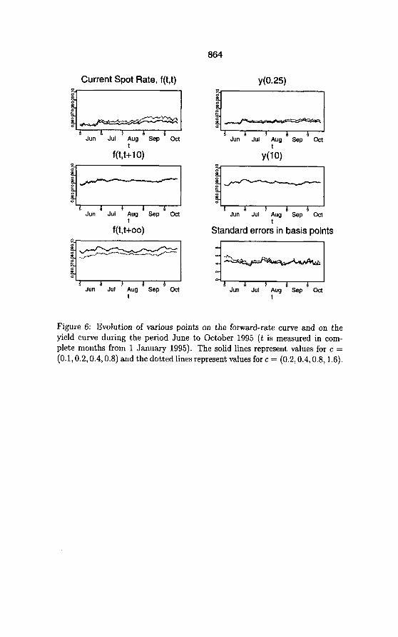
Using the 1988-1993 data (Figure 5), it was found that o = 0.001 (i.e. 10 basis points in the yield) was about right. For the 1995 data (Figure 6) (T = 0.0005 was nearer the mark. This difference is not surprising as prior to 1995 there was a marked coupon effect which the present model for the the forward-rate curve was unable to take account of given that it does not distinguish between income and capital. Never-the-less, it was perhaps surprising that the value of u = 0.001 was so low.

The effect of the choice of u2 was also considered. (It is intended that, like c, u2 should be fixed at the outset.) If there was no prior distribution then the value

862

Current Spot Rate, f(t,t)

Standard error: in basis points

t t

Figure 5: Evolution of various points on the forward-rate curve and on the yield curve during the period 1988 to 1993. The solid lines represent values for c = (0.1,0.2,0.4,0.8)andthedottedlinesrepresentvaluesforc= (0.2,0.4,0.8,1.6).

of u2 would have no effect on the estimates of a or b. If prior distributions are included, there is an effect on the estimates of a and b but this is very insignificant.

Results for 1988-1993 are plotted in Figure 5. (The current spot-rate j(t, t) and the 3-month par-yield ~(0.25) are given to allow comparison with money- market rates and treasury-bill prices.)

It can be seen that there was considerable variation over this period, but this variation appeared to be relatively smooth. Possibly the least variation was observed in the lo-year forward rates and yields.

Several choices for the vector c = (ci, c2,c3,c~) were considered. Of these,

863

c = (0.1,0.2,0.4,0.8) was found to be best over both the 1988-1993 and 1995 periods investigated. Other choices were only slightly worse and an example of one alternative is given in Figures 4 and 5 (c = (0.2,0.4,0.8,1.6)). Although there was not an obvious deterioration in fit, it has already been noted by considering Figure 5 that the long-term forward rate is fairly sensitive to the choice of c. Although this gives some cause for concern, it is unlikely that this problem could be removed through the use of an alternative model, because there will always be a range of possible parameter sets which are almost as good as the optimum and which give a wide variety of log-term forward rates.

Given that the 1995 dataset covers a much shorter period of time there is much less variability to observe in the evolution of the forward rate curve. However, there was a reasonable amount of randomness from one day to the next. Standard errors are considerably smaller than those in Figure 5 because the coupon effect had been almost entirely removed by this time.

4.1 Possible constraints

Two constraints on the forward-rate curve were considered:

(a) that the estimated yield on a three-month zero-coupon bond be equal to the 3-month Treasury-Bill rate given in the FT London Money Rates table (that is, Ji.25 f(t,t + s)ds) = log[l + T&i/4(t)] and T&i is the mid-point S-month Treasury-Bill rate);

(b) that the yield, $(oo), on an irredeemable stock, is equal to the mean of the gross redemption yields on 4% Consols and on 2.5% Treasury.

Inserting the constraint on 3-month zero-coupon bonds was found to increase the errors in the predicted yields by about 2 basis points during 1995. Trea- sury Bill data was not readily available for the period 1988 to 1993. It has been suggested that an alternative to the Treasury Bill rates is the 3-month Commercial Deposit rate minus 20 basis points, but this has yet to be tested.

Pegging down the long-term gross redemption yield was found to make very little difference to the goodness of fit implying that this constraint is acceptable leaving optimization over 4 rather than 5 parameters. To satisfy the constraint it is necessary to specify, for example, the values of bi, bz, b3 and bq and solve numerically for the value of a which gives the correct yield on irredeemable stocks. This numerical step itself requires additional computional effort re- ducing the benefits of the reduction in the number of parameters to maximize over.

Current Spot Rate, f(t,t)

864

~(0.25)

Jun Jut Aug Sep Ott t

Jun Jul Aw Sep Ott t

Jun Jul Aw Sep Ott t

4 1 9 1 A Jun Jul Aw Sep Ott

t

Jun Jul Aug Sep Ott

Standard error: in basis points

Jun Jul Aw Sep Ott t

Figure 6: Evolution of various points on the forward-rate curve and on the yield curve during the period June to October 1995 (t is measured in com- plete months from 1 January 1995). The solid lines represent values for c = (0.1,0.2,0.4,0.8) and the dotted lines represent values for c = (0.2,0.4,0.8,1.6).

Standard errors in basis points =-I I

Jun Jul Aw sep oci t

Jun Jul Aug Sep oci t

Jun Jul Aug Sep 0~3 t

865

Current Spot Rate, f(t,t)

Jun Jul Aw Sep Ott 1

Jun Jul Aw Sep act t

Y (00)

fyizyzy

Jun Jul 4 Sep Ott I

Figure 7: Evolution of various points on the forward-rate curve and on the yield curve during the period June to October 1995 (t is measured in months from 1 January 1995). Results with (solid line) and without (dotted line) irredeemable stocks.

It was generally felt amongst the members of the Fixed Interest Indices Work- ing Party that even 4% Consols and 2.5% Treasury have unreliable prices which are out of line with the rest of the market. On that basis it would be appropri- ate to either ignore all irredeemable stocks or to specify a higher variance in the price of an irredeemable. The fitting exercise was therefore repeated, with all irredeemable stocks removed from the data. The results of this are plotted in Figure 7.

There are two points to make here. First, it can be seen that when the consols’ yield is out of line with that of the more-frequently-traded long-dated stocks (for example, in June 1995) the fit of the model is improved. Furthermore, as is described below removing the irredeemables improves the performance of the model in the Runs Test. Second, we can observe that the long-term forward rate f(t, t + co) is less stable when the irredeemable stocks are removed. This

866

indicates that there is some value added by the irredeemable stocks.

4.2 Other tests of goodness of fit

It has already been pointed out that Root Mean Squared Errors (RMSE) were found to be about 10 basis points (1988-1993 data, significant coupon effect) or 4 to 5 basis points (1995 data, no significant coupon effect) (Figures 4, 5 and 6). This represents a significant improvement over the existing yield-curve model without the necessity of adding further parameters. The RMSE in the case of the new statistical model is, in fact approximately equal to (but larger than) the derived RMSE for the estimated errors in the gross redemption yields. (In fact, if we excluded the l/3200’ from the variance of log Pi in the current model then the RMSE plotted here would be equal to the RMSE in the fitted yields.)

The Runs Test was also applied to the results to test for independence of the residuals. In this test we consider the residuals zi = yi - &, and let n1 be the number of positive and n2 be the number of negative residuals. If the estimated curve provides a poor fit then, we may, for example, observe that all long-dated stocks all have yields which are below their estimated values, and the number of runs would be quite low.

As an example, suppose z = (1.1,0.6, -0.3, -0.7, -0.2,0.7, -0.1,0.6). We first translate this into -t’s and -‘s: that is, (+ + - - - + -+). A sequence of +‘s (minimum length 1) then counts as one run. So then the number of runs here is 5.

If the residuals are independent with Pr(zj > 0) = ni/(ni + n2) (that is, the null hypothesis) then we can derive the distribution of the number of runs. If the observed value is consistently too low then the model may be considered to have provided a poor fit. If the number of runs calculated each day occasionally looks too low then this is not a problem, since random variation will dictate that this will happen occasionally.

The Runs test was applied to each of the 100 days included in the 1995 data and the results are plotted in Figure 8. The plot gives results for the two cases with (solid line) and without (dotted line) the irredeemable stocks. The plot gives percentage points under the null hypothesis for the observed number of runs using the Normal approximation to the number of runs. The following observations are made:

l As one might expect, there is a high degree of correlation from one day

867

5 June

6 July ’ August

6 September ’ October

t

Figure 8: 1995 data. Approximate p-values (calculated separately for each day) for the numbers of runs based upon the null-hypothesis that residuals zi are independently distributed with Pr(z; > 0) = nr/(nr + na).

to the next.

l There are periods when the numbers of runs is relatively low. The worst cases occurred when there were 10 runs against an expected number of 18.

l Generally, however, the numbers of runs were not so low as to give seri- ous grounds for concern. The outcome is reasonably acceptable without being too good. With more experience we could find that the situation is better or worse but certainly, because of serial correlations, we have an inadequate set of data at the moment.

l Removing the irredeemables increases the number of runs indicating that their removal is worthwhile.

Residuals were also tested for correlation with the size of the coupon. The observed correlation coefficients for the 1988 to 1993 data were positive and very significant as we would expect. On-the-other-hand when we consider the 1995 data we find the the residuals showed no significant correlation with coupon, demonstrating that the imminent changes to the taxation of gilts has already been factored into the pricing structure of fixed interest bonds.

868

4.3 Comment on the choice of model

In section 3.5 it was remarked that the root-mean-squared-error with the new model hovers around 4 or 5 basis points. This was achieved with a 5-parameter model (the long-term forward rate plus m = 4 exponential terms). It was found that m = 4 was necessary to fit the data well on all dates examined. With m = 2 the RMSE was much higher at about 10 basis points during 1995. With m = 3 the RMSE only a little above that the m = 4 on average but there was some evidence that the differences could vary significantly. On some days the differences would be negligible, while on other days m = 3 would give a significantly worse fit. Since m = 4 was required for a good fit on a limited number of days it was felt that this should be used rather than m = 3.

5 Catastrophic Jumps

The new forward-rate model was investigated for the existence of multiple maxima. If more than one maximum exists then clearly there would still be the potential for catastrophic jumps in the future.

Using the new model the logarithms of the prices are not linear functions of the five parameters. If this was the case then we could say for sure that there will always be a single maximum because maximizing the likelihood would be equivalent to maximizing a quadratic function of the five parameters. This would be a result of the switch from a non-linear function to one which is linear in the 5 parameters a and the b;. Since this is not the case it is difficult to say with certainty that there are no multiple maxima, but it is strongly suspected that this is the case. There are two reasons for why this might be.

First, a number of specific dates were considered on an individual basis. For each date 100 starting points for the optimization were chosen at random. In each of these cases the algorithm converged to the same maximum.

Second, one can argue that multiple maxima are less likely to exist than before on the following grounds. If the market was made up entirely of zero-coupon stocks then the logarithms of the prices would be linear functions of the pa- rameters. Furthermore, if we ignored the prior distribution the the problem would reduce to maximizing a quadratic function. So in this special case it is known that there would be a unique maximum. In the earlier model, even in the zero-coupon bond case the Dobbie and Wilkie (1978, 1979) model would still be non-linear and we know that multiple minima exist in that particular example. As we move (in a continuous sense) away from this ideal position

869

to one which includes small coupons then, at first, continuity tells us that the likelihood surface will have more-or-less the same shape as before and, in par- ticular, will have only one maximum. As we increase the significance of the coupons further this may cease to be the case. But we can say that at least there will be a unique maximum if there are only low-coupon (in some sense) stocks. What is not clear is whether or not this is true also for markets with higher coupons, or, if it multiple maxima do turn up, is this beyond reasonable coupon rates.

Further investigation will need to be done here.

Acknowledgements

The author would like to thank the various members of the Fixed Interest In- dices Working Party. In particular, George Gwilt first suggested the use of the exponential class of forward-rate curves as an alternative to yield curves, while Geoff Chaplin, Keith Feldman and David Wilkie provided useful discussion of the results.

870

References

Anderson, N., Breedon, F., Deacon, M., Derry, A. and Murphy, G. ( 1996) Estimating and interpreting the yield curve. Wiley, Chichester.

Clarkson, R.S. (1979) A mathematical model for the gilt-edged market. Journal of the Institute of Actuaries 106, 85-132.

Dobbie, G.M. and Wilkie, A.D. (1978) The FT-Actuaries Fixed Interest Indices. Journal of the Institute of Actuaries 105, 15-27.

Dobbie, G.M. and Wilkie, A.D. (1979) The FT-Actuaries Fixed Interest Indices. Transactions of the Faculty of Actuaries 36, 203-213.

Heath, D., Jarrow, R. and Morton, A. (1992) Bond pricing and the term structure of interest rates: a new methodology for contingent claims valuation. Econometrica 60, 77-105.

McCutcheon, J.J. and Scott, W.F. (1986) An Introduction to the Mathematics of Finance. Heinemann, Oxford.

Nelson, C.R., and Siegel, A.F. (1987) P arsimonious modeling of yield curves. Journal of Business 60, 473-489.

Poston, T. and Stewart, I.M. (1978) Catastrophe theory and its applications. Pitman, London.

Svensson, L.E.O. (1994) Estimating and interpreting forward interest rates: Sweden 1992-1994. Working paper of the International Monetary Fund 94.114, 33 pages.

Vasicek, 0. (1977) An equilibrium characterization of the term structure. J. Financial Economics 5, 177-188.