anewhybridmethodologyforcooperative ... fileof radial basis function networks ... abstract this...

Soft Comput (2007) 11:655–668DOI 10.1007/s00500-006-0128-9

ORIGINAL PAPER

A new hybrid methodology for cooperative-coevolutionary optimizationof radial basis function networks

A. J. Rivera · I. Rojas · J. Ortega · M. J. del Jesus

Published online: 8 August 2006© Springer-Verlag 2006

Abstract This paper presents a new multiobjectivecooperative–coevolutive hybrid algorithm for the de-sign of a Radial Basis Function Network (RBFN). Thisapproach codifies a population of Radial Basis Func-tions (RBFs) (hidden neurons), which evolve by meansof cooperation and competition to obtain a compact andaccurate RBFN. To evaluate the significance of a givenRBF in the whole network, three factors have been pro-posed: the basis function’s contribution to the network’soutput, the error produced in the basis function radius,and the overlapping among RBFs. To achieve an RBFNcomposed of RBFs with proper values for these qualityfactors our algorithm follows a multiobjective approachin the selection process. In the design process, a FuzzyRule Based System (FRBS) is used to determine thepossibility of applying operators to a certain RBF. Asthe time required by our evolutionary algorithm to con-verge is relatively small, it is possible to get a furtherimprovement of the solution found by using a local min-imization algorithm (for example, the Levenberg–Mar-quardt method). In this paper the results of applying ourmethodology to function approximation and time seriesprediction problems are also presented and comparedwith other alternatives proposed in the bibliography.

A. J. Rivera (B) · M. J. del JesusDepartment of Computer Science,University of Jaén, Jaen, Spaine-mail: [email protected]: http://wwwdi.ujaen.es/∼arivera

I. Rojas · J. OrtegaDepartment of Computer Architecture andComputer Technology, University of Granada,Granada, Spain

Keywords Cooperative–coevolution ·Soft-computing techniques · RBF networks ·Fuzzy rule based system · Function approximation

1 Introduction

The extensive research work carried out on the designof neural networks (Haykin 1999; Lipmann 1987; Platt1991; Widrow and Lehr 1990), and more specifically onRBFNs, reveals the difficulty of this task and the ab-sence of general mechanisms to automatically set thenetwork parameters. In this field, the importance of soft-computing (Tettamanzi and Tomassini 2001) must behighlighted as one of the lines of development with thebest results. Evolutionary Computation (EC) (Schwefel1995) is one of the soft-computing strategies frequentlyapplied to design neural networks.

According to Potter and De Jong (2000), it can bedifficult to solve certain types of problems using evo-lutionary computation, especially when an individualrepresents a complete solution (i.e. a net) made of inde-pendent subcomponents. In these situations, the indi-viduals’ size can imply a premature convergence of thepopulation and specific operators and mechanisms mustbe used to avoid it. Moreover, the role of good (or bad)independent subcomponents has not been taken intoconsideration in an individual solution or net. In thesescases, it is suitable to extend the basic computationalmodel of evolution to provide a frame where the sub-components evolve and cooperate to reach a solution inan independent way and to maintain the diversity.

A solution for this problem is Cooperative Coevolu-tion (Potter and De Jong 2000; Rosin and Belew 1997), in

656 A. J. Rivera et al.

which the individuals in the population represent only apart of the solution and evolve in parallel, not only com-peting to survive but also cooperating to find a commonsolution at the same time. Compared with other evolu-tionary procedures, this new approach has the advan-tage of being less computationally complex and thusmore cost effective since an individual does not repre-sent the whole solution but only a part of it. The keypoint in a cooperative coevolutionary procedure is thecredit assignment or the allocated fitness to each individ-ual according to its contribution to the final solution.

Due to the novelty of this field and the difficulties ofan adequate implementation of the above aspects, fewproposals have been carried out in cooperative coevo-lution for the design of neural networks. A first exam-ple would be the Smalz and Conrad model (Smalz andConrad 1994), where multilayer networks are built bysubpopulations of nodes and the credit assignment isdone according to the compatibility of each populationwith different networks. The Symbiotic Adaptive NeuroEvolution (SANE) developed by Moriarty and Miikku-lainen (1997) is based on the coevolution of nodes, whichtake part in different candidate networks. The creditassignment to each node is done by using the averageefficiency of the five best networks it participates in. An-other interesting paper that applies cooperative coevo-lution to design neural networks can be shown in garciaet al. (2002). In this paper, subcomponent credit assign-ment is determined through a multiobjective coopera-tive coevolutionary technique which measures factorssuch as their efficiency and complexity.

In RBFNs, the response of the hidden neurons islocalized, and they can be optimized by means of coop-erative coevolutive methods. The main contribution ofthis paradigm is to direct the search using a credit assign-ment for each RBF based on its contribution to the per-formance of the network as a whole and also based onits importance.

In this paper a new hybrid cooperative coevolutivemethodology for optimization of RBFNs is presented.To carry out the credit assignment three quality factorswhich define the role of each RBF have been defined: thebasis function’s contribution to the network’s output; theerror in the basis function radius; and the overlapping ofRBFs. To combine them in a proper way a multiobjec-tive technique is incorporated. Moreover, an FRBS isused to determine the application of different operatorsover an RBF.

The organization of this paper is as follows. Section 2introduces the RBFNs and describes different alterna-tives for the optimization of the network parameters.In Sect. 3, the details of the proposed multiobjectivecooperative coevolutionary algorithm are described.

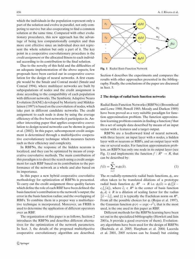
Fig. 1 Radial Basis Function Network

Section 4 describes the experiments and compares theresults with other approaches presented in the bibliog-raphy. Finally, the conclusions of the paper are discussedin Sect. 5.

2 The design of radial basis function networks

Radial Basis Function Networks (RBFNs) (Broomheadand Lowe 1988; Powell 1985; Moody and Darken 1989)have been proved as a very suitable paradigm for func-tion approximation problem. The function approxima-tion learning problem consists in finding a function f thatfits a set of sample data described by means of an inputvector with n features and a target output.

RBFNs are a feedforward kind of neural network,with three layers: an input layer with n nodes, a hiddenlayer with m neurons or RBFs, and an output layer withone or several nodes. For function approximation prob-lem, an RBFN has only one node in its output layer (seeFig. 1) and implements the function f : Rn → R, thatcan be described by:

f (�x) =m∑

i=1

wiφi(�x). (1)

The m radially-symmetric radial basis functions, φi, areoften taken to be translated dilations of a prototyperadial basis function φi: Rn → R i.e. φi(�x) = φi

(∥∥�x −ci

∥∥/di

), where �ci ∈ Rn is the center of basis function

φi, di ∈ R is a dilation of scaling factor for the radius∥∥�x − �ci∥∥, and ‖‖ is typically the Euclidean norm on Rn.

From all the possible choices for φi (Rojas et al. 1997),the Gaussian function φ(r) = exp(−r2), that is the mostused, is the one used in this paper as RBF.

Different methods for the RBFNs learning have beenset out in the specialized bibliography (Howlett and Jain2001a, b provide a good overview of them). Evolution-ary algorithms have been used for the design of RBFNs(Buchtala et al. 2005; Harpham et al. 2004; Lacerdaet al. 2001, 2005 reviews can be found) but existing

A new hybrid methodology for cooperative-coevolutionary optimization 657

approaches typically suffer from the problems of a highruntime and a premature convergence in local minima.Those are both objectives to reach in any evolutionaryproposal for the design of RBFNs.

In Butchala et al. (2005) analyze the combination ofevolutionary algorithms and RBFNs and consider thatthis hybridization can be classified in different categoriesrelated to the aspect that is optimized:

1. The computation of weights, i.e., centers and radiiof RBFs and/or output weights.

2. The determination of the architecture of RBFN.3. The feature selection for the RBFN.4. The combination of networks in form of ensembles.

In this paper, the structure of the RBFN is fixed pre-vioulsy and we only consider the evolutionary compu-tation of centers and radii of RBFs. The weights areadjusted by means of Levenberg–Marquardt training.For this problem, in the specialized bibliography differ-ent evolutionary approaches have been presented withindividuals which are complete RBFNs or single RBFswhich constitute a network.

The former idea is investigated in Rivas et al. (2002),in which the genetic algorithm evolves a populationof RBFNs to determine the network parameters. Inthis proposal the SVD algorithm (Golub and Van Loan1996) was used to calculate the weights of the net. In apaper by González et al. (2003), this codification schemeis used in a multiobjective genetic algorithm which insome of its stages, also employs conventional techniquessuch as clustering algorithms, Orthogonal Least SquaresOLS (Chen et al. 1999) or Singular Value Decomposi-tion (SVD) (Golub and Van Loan 1996). In thisapproach the Levenberg-Marquardt algorithm (Marqu-ardt 1963) is used to further minimize the approximationerror.

The evolution of single RBFs is investigated by White-head and Choate (1996) where a cooperative-competi-tive evolution of centers and radii is proposed. In theirgenetic algorithm, selection operates on individual RBFsrather than on whole networks and the entire populationcorresponds to a single RBFN and the credit assignmentto each individual is based on its contribution to the per-formance of the network as a whole and on the RBFweight. With this credit assignment strategy, it is shownthat it is possible to maintain the diversity in the pop-ulation. In this approach, the algorithm Singular ValueDecomposition (SVD) (Golub and Van Loan 1996) isalso applied to determine more accurate values for theweights of the network.

Although evolutionary alternatives to design RBFNsare frequent, few cooperative coevolutionary procedures

have been implemented up to now, due to the problemsarising in their development, especially with the creditassignment strategy which must promote competitionamong similar RBFs and cooperation among the differ-ent ones at the same time.

In this paper (an extended version can be found byRivera 2003) we present a new hybrid methodology forthe optimization of RBFNs based on a cooperative–coevolutionary algorithm. The proposal defines threecriteria for the credit assignment, establishes a multiob-jective selection for the individuals and uses an FRBSfor the application of the operators in the evolution-ary process. We have presented other coevolutionaryapproaches for this problem. In Rivera et al. (2003)the fitness of an RBF was calculated as a combinationof different factors (a factor which takes into accountits weight, a factor that measures its closeness to worstapproximated points and a factor which quantifies theoverlapping among RBFs), probabilistic rules are usedto apply the operators and a monoobjective approach isconsidered. In the paper (Rivera et al. 2003), a prelimi-nary approach was presented, with different criteria toevaluate an RBF.

3 A new approach for the optimization of RBF usinga multiobjective cooperative–coevolutive algorithm

In the approach proposed in this paper each individ-ual represents a basis function (RBF), and thereforeforms only a part of the solution to the problem underanalysis. Thus the entire population is responsible forthe final solution. This allows for an environment wherethe individuals cooperate towards a definitive solution.However, they also compete for survival, since if theirperformance is poor, they will be eliminated.

One of the most important contributions of this pro-posal is the evaluation of each basis function by means ofthree criteria related with its role in the complete RBFN.These quality factors allow for an accurate evaluation ofits participation within the network, or more generally,the assigned credit of each RBF to the final solution. Tobe precise, the three factors are the following ones:

• ai: which measures the basis function’s contributionto the network’s output.

• ei: that calculates the local error produced in thebasis function radius.

• oi: which evaluates the degree of overlapping ofRBFs. This objective will be used to maintain thediversity of the population.

The three objectives are important to obtain accurateRBFNs, with a good local and global performance and


composed of a set of RBFs which describe informationabout different areas of search space.

Another important characteristic of our approach isthat the way to combine these objectives is to evaluatethe RBFs. In a previous approach (Rivera et al. 2001), wecalculate the credit assignment as a weighted expressionof characteristic parameters. This proposal has two dis-advantages: the subjective determination of the weightsand the possibility of obtaining a solution with a highvalue in one objective but very low values in the others.In this RBFN design process with a cooperative coe-volutive approach it is most suitable to consider eachobjective in an independent way and to apply multiob-jective theory to sort the RBFs.

To complete the hybrid bio-inspired architecture, aFuzzy Rule Based System (FRBS) is used as the mainstrategy in order to decide the operators’ applicationover a certain RBF. The inputs for the FRBS are thevalues of the objectives previously defined. The use ofan FRBS for this task let us include in our cooperativecoevolutive methodology the knowledge of an experton the RBFN design.

The RBF network obtained from the hybrid bio-inspired procedure here described provides a solutionto the problem of function approximation from a set ofdata points. This solution has a proper level of accuracyand simplicity (see the results in Sect. 4). Nevertheless,if more accuracy is required, it is possible to improvethe quality of the solution found, by applying a localoptimization procedure. More specifically, the Leven-berg–Marquardt algorithm (Marquardt et al. 1963) hasbeen incorporated to our cooperative coevolutionaryprocedure.

The fact that the cooperative coevolution methodol-ogy we propose, where a population of RBFs and notRBFNs evolve, decreases the computational cost mustbe highlighted (see experimental results in Sect. 4).

It is remarkable that in the evolutionary design ofRBFNs (Buchtala et al. 2005) research field there are notso many coevolutionary approaches. The most impor-tant work is described before by Whitehead and Choate(1996), in which the credit assignment for each RBF isonly based on the weight of the RBF. And, it does notinclude expert knowledge in the evolution.

In the following a detailed description of hybrid mul-tiobjective methodology for cooperative coevolutionaryoptimization of RBFNs is shown.

3.1 Detailed algorithm

As is mentioned previously the complete populationrepresents an RBFN with a number of radial basis func-tions determined by the population size.

Algorithm 1. Detailed algorithm for the design of theRBFNs

1. Initialize RBFN2. Train RBFN3. Evaluate RBFs4. Select the worst RBFs5. Apply operators to the worst RBFs usingan FRBS

6. Substitute the RBFs that were eliminated7. Train RBFN8. If the stop− condition is not verifiedgo to step 3, else go to 9

9. Apply Levenberg− Marquardt

The main steps of the proposed algorithm are shownin Algorithm 1. These steps are explained in the follow-ing subsections:

3.1.1 Initializing the population

A simple process is used to define the first network tobegin with. According to the population size (i.e. thenumber of RBFs, m), the centre, ci, for each basis func-tion, φi, in the network is randomly generated by keep-ing a minimum distance with the centres of the basisfunctions already generated. This minimum distance isthe half of the radius that the m basis functions of thenetwork would have if they were uniformly distributedand covering the whole input space without overlapping.

Initially, the radius will be set to a random valuearound the average distance from each RBF to the near-est neighbour RBF, and the weights are set to 0.

3.1.2 RBFN training

There are several methods like LMS (Widrow and Lehr1990), SVD (Golub and Van Loan 1996), etc. to adaptthe weights of a RBFN. In our proposal LMS is usedbecause it is a simple and efficient (in computationalcost) technique to calculate these weights. In addition,this technique can obtain a more or less precise solution,depending on the value of parameter alfa or the timesthat the method is applied. This is a suitable characteris-tic in our algorithm, because in the main loop we do notwant a very accurate solution and we can save compu-tational time. At the end of the algorithm we apply theLevenberg–Marquardt algorithm to reach a high qualitysolution.

In this stage, the LMS algorithm is executed over thetraining set until the error does not decrease for twoconsecutive iterations.


3.1.3 Evaluating RBFs

From the coevolutionary point of view of this work, acredit assignment mechanism is required to evaluate therole of each base function in the whole network. For thispurpose, three parameters for each RBF φi are defined,taking into account the local behaviour of an RBF:

• ai: measures the contribution of the base function tothe output of the network.

• ei: gives the error in the basis function radius.• oi: evaluates the overlapping among RBFs.

The contribution, ai, of the RBF φi, i = 1, . . . , m, isdetermined by considering its weight wi and the num-ber of points of the training set inside its radius, pri.

ai = α· |wi| · pri1m

∑mj=1 prj

, (2)

where the parameter α allows the normalization of ai

inside the interval [0,1]. This normalization is requiredto assure an adequate FRBS performance.

The error measure, ei, for each RBF φi, is obtainedfrom the normalized root mean square error nrmsei ofthe data points inside the radius of the RBF, as well asthe standard deviation error, S(ei), also defined in theradius of the RBF.

ei = β · nrmsei · S(ei)

1m

∑mj=1 S(ei)

. (3)

Again, to be able to analyze the error values throughan FRBS, they have to be moved around the interval[0, 1] with the parameter β.

Any overlapping among the RBF φi and other RBFsis quantified by using the parameter oi. This parame-ter is calculated by taking into account the fitness shar-ing (Golberg and Richardson 1987) methodology, whoseaim is to keep the diversity in the population, thus main-taining the bases of the coevolutionary algorithms.

The parameter oi is expressed as:

oi =m∑

j

oij, (4)

where oij measures the overlapping among the RBFsφj, j = 1, . . . , m, and φi, is calculated as:

oij ={(

1 − ∥∥φi − φj∥∥/

di

)if

∥∥φi − φj∥∥ < di

0 otherwise, (5)

where || · || is the Euclidean distance between the twobasis functions, and di is the radius of the basis functionφi.

In opposite to the calculation of the previous param-eters, the expression to determine the values of oi pro-vides an absolute measure of the neurons overlapping,since it does not depend either on the problem, or onthe current network. The parameters oi can be directlyanalyzed using an FRBS without applying any kind ofdisplacement.

Figure 2 shows the behaviour of the parameter oij.In a the value of oij is 0 because there is not overlapbetween i and j. However in b the value of oij is greaterthan 0, and therefore the overlap between the hiddenneurons is detected.

3.1.4 Sorting and selecting basis functions

An appropriate way to sort the basis functions musttake into account the three parameters that characterizetheir contribution to the final solution. A multiobjective(Coello et al. 2002) approach (not based in the searchfor the Pareto optimal front) has been used to take intoaccount these three parameters, which have been con-sidered as different objectives.

To sort the population, first the worst basis functionφi is selected, which is the one with the worst values forthe three parameters (the lowest value for ai, the high-est value for ei, and the highest value for oi). If thereis no such basis function, the worst RBF is randomlychosen between the RBFs with the worst values in twoof the three parameters. If such basis function does notexist, any of the parameters is randomly chosen and thebasis function that presents the worst value within thisparameter is selected as the worst basis function. Thisprocedure is repeated with the remaining RBFs until allthe basis functions have been sorted.

Once the sorting procedure is applied, the m/2 worstfunctions are selected and the operators described in thefollowing subsection are applied to these selected RBFs.

3.1.5 Applying the operators to the set of worst basisfunctions

In the research field of cooperative coevolutive learningit is frequent to use only the mutation operator (Rechen-berg 1973) to explore the search space. Moreover, in theevolutionary design of RBFNs the crossover operatorcan be destructive when the individuals are not made byindependent subcomponents as in our case (Angelineet al. 1994; Yao 1999).

Taking this into account, in this proposal, only twooperators are defined to be applied to the selected RBFs:an operator that eliminates RBFs, and an operator thatadapts the selected RBF to the zone where it is situated.These operators exploit the local information that can


Fig. 2 Example of RBFs. a With no overlap. b With overlap


be obtained from the contribution of each basis func-tion to the network. A more detailed explanation of theproposed operators is given below:

• Operator REMOVE: It simply eliminates an RBF.• Operator ADAPT: This operator adapts the RBF to

the examples belonging to the zone where the RBFis allocated. To do this, the output of the networkis evaluated at the training points inside the radiusof the RBF, and according to this output, the centreand the radius of the RBF are modified. These mod-ifications are based on the LMS algorithm (Widrowand Lehr 1990).

As has been said, to decide the application of an opera-tor to a basis function, an FRBS (Mendel 1995) is used.The goal of this fuzzy system is to take decisions aboutthe operators according to expert knowledge and thebehaviour of the RBF in the RBFN.

The three objectives previously defined characterizethe contribution of each base function to the network,and its relation with the rest of the base functions. In thisway, the parameters ai, ei and oi are used as inputs inthe fuzzy system. These inputs are considered as linguis-tic variables vai, vei and voi. Moreover, two outputs aredefined. The output premove is the probability of applyingthe operator REMOVE, while the output padapt deter-mines the probability of applying the operator ADAPT.

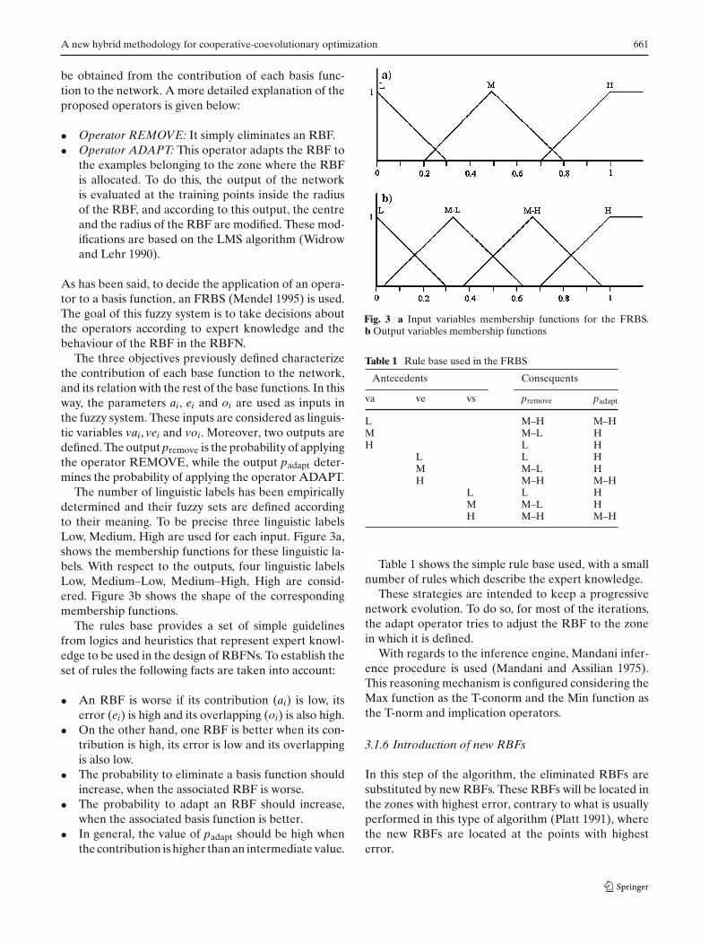
The number of linguistic labels has been empiricallydetermined and their fuzzy sets are defined accordingto their meaning. To be precise three linguistic labelsLow, Medium, High are used for each input. Figure 3a,shows the membership functions for these linguistic la-bels. With respect to the outputs, four linguistic labelsLow, Medium–Low, Medium–High, High are consid-ered. Figure 3b shows the shape of the correspondingmembership functions.

The rules base provides a set of simple guidelinesfrom logics and heuristics that represent expert knowl-edge to be used in the design of RBFNs. To establish theset of rules the following facts are taken into account:

• An RBF is worse if its contribution (ai) is low, itserror (ei) is high and its overlapping (oi) is also high.

• On the other hand, one RBF is better when its con-tribution is high, its error is low and its overlappingis also low.

• The probability to eliminate a basis function shouldincrease, when the associated RBF is worse.

• The probability to adapt an RBF should increase,when the associated basis function is better.

• In general, the value of padapt should be high whenthe contribution is higher than an intermediate value.

Fig. 3 a Input variables membership functions for the FRBS.b Output variables membership functions

Table 1 Rule base used in the FRBS

Antecedents Consequents

va ve vs premove padapt

L M–H M–HM M–L HH L H

L L HM M–L HH M–H M–H

L L HM M–L HH M–H M–H

Table 1 shows the simple rule base used, with a smallnumber of rules which describe the expert knowledge.

These strategies are intended to keep a progressivenetwork evolution. To do so, for most of the iterations,the adapt operator tries to adjust the RBF to the zonein which it is defined.

With regards to the inference engine, Mandani infer-ence procedure is used (Mandani and Assilian 1975).This reasoning mechanism is configured considering theMax function as the T-conorm and the Min function asthe T-norm and implication operators.

3.1.6 Introduction of new RBFs

In this step of the algorithm, the eliminated RBFs aresubstituted by new RBFs. These RBFs will be located inthe zones with highest error, contrary to what is usuallyperformed in this type of algorithm (Platt 1991), wherethe new RBFs are located at the points with highesterror.


The above indicated zones with the highest error aredetermined by using the points that are outside any basisfunction radius. From these points, the one with the high-est error will be the new centre of the one with a radiusequal to the average of the RBFs radius. The error in thiszone is calculated as the normalized root mean squarederror (nrmse) of the points inside the zone.

The new RBFs will be iteratively introduced inthese zones with higher error until the population iscompleted.

4 Experimental results

This section provides some experimental results ob-tained by the proposed algorithm in function approx-imation and time series forecasting problems.

For the experimentation the following conditions areestablished:

• The stop condition for the algorithm is a maximumnumber of iterations determined in a dynamical way:first, stop condition is set to 300 iterations. But if inthe last 50 iterations an improvement of the error isobtained, the new stop condition is increased by 50.

• The solution is the RBFN chosen is the RBFN withthe best error obtained during the entire run.

• The error used to measure the approximation of ourmodel is the nrmse.

• The results are obtained after 30 runs of the method.

4.1 Function Approximation

The function approximation problem can be defined asthe problem of estimating an unknown function, f, froma set of training examples: (�xk; zk); k = 1, 2, . . . , K; withzk = f (�xk) ∈ R, and �xk ∈ Rn.

In the following subsections the functions used andthe results obtained are shown.

Example 1 First, a 1-D target function is considered:

dickerson(x)=3x(x−1)(x−1.9)(x+0.7)(x+1.8),

x ∈ [−2.1, 2.1]. (6)

This function was proposed by Dickerson and Kosko(1996), where a hybrid neuro-fuzzy system is proposedusing ellipsoidal rules to approximate the original func-tion. This function was also used by Pomares et al.(2000), where a robust algorithm for the identificationand optimization of a fuzzy system is proposed.

In this experimentation, to evaluate the behaviour ofthe proposed algorithm, a training set of 500 samples anda test set of 1,000 samples of the dickerson(x) function

Fig. 4 Comparison of the results obtained for the TrainingNRMSE using different numbers of RBFs or Rules for the bench-mark function Dickerson

are generated by using inputs that have been randomlysampled from the interval where the function is definedas by González et al. (2003).

Figure 4 and Table 2 show the results of the proposedalgorithm in the approximation of dickerson(x) func-tion and the comparison with other methods for directsynthesis of fuzzy systems and neural networks reportedin the bibliography. The notation used is the following:m stands for the number RBFs or rules (depending onthe model) in the solution obtained; np is the numberof parameters learned by the algorithm; MSE stands formean square error and NRMSE is the normalized rootmean square error. In this case error for the trainingset is showed because only these results are found inthe specialized bibliography. Anyway, we have checkedthat these results are very similar to test results for ouralgorithm.

From these data, it is clear that the inclusion of newRBFs decreases the error index. The proposed algo-rithm outperforms the results of other procedures pre-sented by Dickerson and Kosko (1996), Pomares et al.(2000), Rives et al. (2002) and gives similar results tothe error indexes by González et al. (2003). Neverthe-less, the algorithm presented here is much simpler andhas a lower computational cost (see results in Sect. 4.3)because (González et al. 2003) uses traditional evolu-tionary computation (an individual is a complete RBFN)or complex mutation operators based on Singular ValueDecomposition (SVD) and Orthogonal Least Squares(OLS).

Example 2 In this example the bidimensional functionapproximation problem is considered. The two selected


Table 2 Comparison of the proposed algorithm with other methods for direct synthesis of neuro-fuzzy systems to approximate thetarget function dickerson (x)

Algorithm m np MSE NRMSE

Dickerson and Kosko (1996) Different weights for rules wk = 1 6 – 94.65 –wk = 1/vk 28.25 –wk = 1/v2

k 10.53 –Not supervised 7.927 –Supervised 3.069 –

Pomares et al. (2000) 5 8 5.01 0.336 10 1.35 0.177 12 0.46 0.10

González et al. (2003) 3 9 5.57 ± 0.00 0.3455 ± 0.00004 12 0.99 ± 0.49 0.1415 ± 0.03905 15 0.30 ± 0.02 0.0797 ± 0.0023

Rivas et al. (2002) 8.3 24.9 0.05 ± 0.04 –Proposed algorithm 3 9 3.57 + 0.00 0.2839 ± 0.0000

4 12 1.27 ± 0.38 0.1671 ± 0.02855 15 0.26 ± 0.09 0.0739 ± 0.02396 18 5.7E-3 ± 0.01 0.0036 ± 0.0052

functions, f4 and f7, are defined by the followingequations:

f4(x1, x2) = 1 + sin(2x1 + 3x2)

3.5 + sin(x1 − x2), x1, x2 ∈ [−2, 2], (7)

f7(x1, x2) = 1.9[1.35 + ex1sen(13(x1 − 0.6)2)

·e−x2 sen(7x2)

]x1, x2 ∈[

0, 1]. (8)

f4 function was reported by Cherkassky et al. (1996),where new methods for the design of Multilayer Per-ceptron are introduced. This function was also used byGonzález et al. (2003), and Pomares et al. (2000).

The f7 function is used by Charkassky and Lari-Najafi(1991) as a benchmark to compare the behaviour ofseveral paradigms applied to function approximation,such as Projection Pursuit (PP) (Frideman 1981), Multi-variate Adaptive Regression (MARS) (Friedman 1991),Constrained Topological Mapping (CTM) and Multi-layer Perceptron (MLP). This function was also usedas a benchmark by Castillo (2000), Cherkassky et al.(1996), and Pomares et al. (2000).

The training set is formed by 400 points randomlyselected from each cell of a 20 × 20 grid partition of theinput space. The test set is built with 961 points obtainedby dividing the input interval into a 31 × 31 grid. Thetraining and test sets are similar to the ones used byCherkassky et al. (1996) and González et al. (2003).

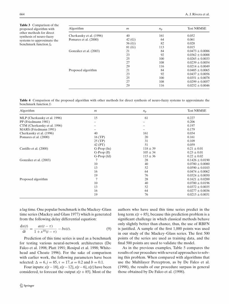
Tables 3, 4 and Fig. 5 compare the proposed algo-rithm with other methods presented in the bibliography.It is important to note that the methodology presentedby Pomares et al. (2000) gives an approximation withvery low error due to the small number of non-linear

Fig. 5 Comparison of the result obtained for the Test NRMSEusing different numbers of RBFs or Rules for the benchmarkfunction f 7

parameters to be optimized. Indeed, there are a greatnumber of linear parameters that can be optimally cal-culated in an FRBS. In this case, the results obtained bythe proposed algorithm are similar to those presentedby Pomares et al. (2000) and González et al. (2003) andbetter than those obtained in the rest of approaches.

4.2 Time series prediction

Time-series prediction is an important practical problemwhich can be formulated as follows: givenx[t−(n−1)�], x[t−(n−2)�], . . . , x[t−�], x[t] determinex[t + j], where n and j are fixed positive integers and � is


Table 3 Comparison of theproposed algorithm withother methods for directsynthesis of neuro-fuzzysystems to approximate thebenchmark function f4

Algorithm m np Test NRMSE

Cherkassky et al. (1996) 40 161 0.052Pomares et al. (2000) 42 (G) 64 0.061

56 (G) 82 0.02881 (G) 113 0.015

González et al. (2003) 21 84 0.0473 ± 0.008623 92 0.0362 ± 0.008825 100 0.0265 ± 0.003327 108 0.0239 ± 0.005429 116 0.0214 ± 0.0049

Proposed algorithm 21 84 0.0485 ± 0.006523 92 0.0437 ± 0.005625 100 0.0351 ± 0.007827 108 0.0299 ± 0.005729 116 0.0252 ± 0.0046

Table 4 Comparison of the proposed algorithm with other methods for direct synthesis of neuro-fuzzy systems to approximate thebenchmark function f7


MLP (Cherkassky et al. 1996) 15 61 0.227PP (Friedmann 1981) – – 0.206CTM (Cherkassky et al. 1996) – – 0.197MARS (Friedmann 1991) – – 0.179Cherkassky et al. (1996) 40 161 0.034Pomares et al. (2000) 16 (TP) 20 0.161

25 (TP) 31 0.10942 (PT) 51 0.059

Castillo et al. (2000) G-Prop (fn) 118 ± 39 0.21 ± 0.01G-Prop (fl) 105 ± 34 0.23 ± 0.01G-Prop (fd) 115 ± 36 0.22 ± 0.02

González et al. (2003) 7 28 0.1426 ± 0.019010 40 0.0780 ± 0.008013 52 0.0590 ± 0.010316 64 0.0474 ± 0.006219 76 0.0324 ± 0.0050

Proposed algorithm 7 28 0.1621 ± 0.020010 40 0.0700 ± 0.019613 52 0.0372 ± 0.003516 64 0.0277 ± 0.003619 76 0.0215 ± 0.0031

a lag time. One popular benchmark is the Mackey–Glasstime series (Mackey and Glass 1977) which is generatedfrom the following delay differential equation:

dx(t)dt

= ax(t − τ)

1 + x10(t − τ)− bx(t). (9)

Prediction of this time series is used as a benchmarkfor testing various neural-network architectures (DeFalco et al. 1998; Platt 1991; Rosipal et al. 1998; White-head and Choate 1996). For the sake of comparisonwith earlier work, the following parameters have beenselected: � = 6, j = 85, τ = 17, a = 0.2 and b = 0.1.

Four inputs: x[t −18], x[t −12], x[t −6], x[t] have beenconsidered, to forecast the output x[t + 85]. Most of the

authors who have used this time series predict in thelong term x[t + 85], because this prediction problem is asignificant challenge in which classical methods behaveonly slightly better than chance, thus, the use of RBFNis justified. A sample of the first 1,000 points was usedin our study of the Mackey–Glass series. The first 500points of the series are used as training data, and thefinal 500 points are used to validate the model.

As in the previous examples, Table 5 compares theresults of our procedure with several approaches to solv-ing this problem. When compared with algorithms thatuse the Multilayer Perceptron, as by De Falco et al.(1998), the results of our procedure surpass in generalthose obtained by De Falco et al. (1998).


Table 5 Comparison of the proposed algorithm with other methods for direct synthesis of neuro-fuzzy systems to approximate thebenchmark Mackey–Glass time series prediction for x(t + 85)


MLP + BGA (De Falco et al. 1998) 16 80 0.2666RAN (Platt 1991) ε = 0.1 57 342 0.378

ε = 0.05 92 552 0.376ε = 0.02 113 678 0.373ε = 0.01 123 738 0.374

RAN-GQRD (Rosipal et al. 1998) ε = 0.1 14 84 0.206ε = 0.05 24 144 0.170ε = 0.02 44 264 0.172ε = 0.01 55 330 0.165

RAN-P-GQRD (Rosipal et al. 1998) ε = 0.1 14 84 0.206ε = 0.05 24 144 0.174ε = 0.02 31 186 0.160ε = 0.01 38 228 0.183

Fuzzy System (Bersini et al. 1997) Brute force 10 190 0.108611 206 0.109812 228 0.102613 247 0.223514 266 0.158615 285 0.1028

Incremental 14 266 0.0965Whitehead and Choate (1996) 25 150 0.29

50 300 0.1875 450 0.11

125 750 0.05González et al. (2003) 14 84 0.1977 ± 0.0164

17 102 0.1467 ± 0.017820 120 0.1268 ± 0.017423 138 0.1012 ± 0.013226 156 0.0999 ± 0.019229 174 0.0891 ± 0.0131

Rivas et al. (2002) 72 432 0.177 ± 0.004Proposed algorithm 14 84 0.1675 ± 0.0210

17 102 0.1281 ± 0.009120 120 0.1133 ± 0.012523 138 0.1059 ± 0.013426 156 0.0947 ± 0.010129 174 0.0803 ± 0.0066

Other comparisons can be done with methodologiesbased on RBFNs, such as the classical model RAN (Platt1991), which iteratively builds an RBFN by analyzingthe novelty of the input data. Although the algorithmRAN was improved by Rosipal et al. (1998), givingas the result, the algorithms RAN-GQRD and RAN-P-GQRD, the proposed algorithm improves these meth-ods.

Another interesting algorithm to consider is the onepresented by Whitehead and Choate (1996). This algo-rithm evolves a population of individuals where eachone of these individuals represents an RBF. Therefore,this algorithm corresponds to an approach similar toour procedure, keeping in mind that it also carries outa final minimization of the error by the application ofthe SVD algorithm. Comparing the NRMSE, one can

observe that, although the algorithm offers similar errorvalues to those obtained by our algorithm, it requires ahigher number of RBFs. Regarding the computationalcost, both algorithms can be considered similar.

With regard to the algorithm (González et al. 2003),the differences in error are small; nevertheless it is impor-tant to take into account that the computational cost ofthis algorithm is very high compared with the cost of ouralgorithm.

The results of our procedure are also compared withthose of an algorithm based on a fuzzy system presentedby Bersini et al. (1997). In this paper two different algo-rithms are presented in order to optimize the member-ship functions and the fuzzy system generated: a bruteforce one, and an incremental one. The unstable behav-iour of the brute force is also evident when the number


Fig. 6 Results obtained by different algorithms in the predictionof the long term, x(t + 85), Mackey–Glass time series

of fuzzy rules increases. It is important to note that,although there is a certain similarity among the errorsobtained with those of our procedure, the number offree parameters of the fuzzy models generated by thismethod Bersini et al. (1997) is far greater.

Finally, it is important to note that our procedure isable to find a set of Pareto-optimum solutions that dom-inate all the solutions in the Table 5. This is graphicallyshown in Fig. 6.

4.3 Analysis of the independent phasesand computational cost of the algorithm

Next, the two main phases of the algorithm, the hy-brid bio-inspired phase and the minimization phase, areanalyzed. For this objective both the bio-inspired phaseand the minimization phase are executed from the sameinitialization and the results of the two phases of thealgorithm and the results of the complete algorithm areshown in the Fig. 7.

As can be seen from these data, the bio-inspired phasereaches a good solution near the solution of the com-plete algorithm. Also, this phase has coherent behav-iour and when new RBFs are introduced the RBFNerror decrease. Moreover the standard deviation is low.If only the minimization phase is applied the results arevery bad with incoherent behaviour, where more RBFsdo not imply a better result or where the standard devi-ation in high.

These results also confirm the reliability of the com-plete algorithm. The solutions obtained from the hybridbio-inspired phase are the most suitable because with ahigh probability, the minimization phase reaches practi-cally a global optimum.

Fig. 7 Comparison of the results of the different phases of thealgorithm for the approximation of the function f4. + results of thecomplete algorithm. x results if only Bio-inspired phase is applied.o results if only minimization phase is applied

Fig. 8 Comparison of the mean computational time requiredfor the proposed algorithm for approximating different problems(function of one and two dimensions, the Mackey–Glass time se-ries), compared with the approach presented by Gonzalez et al.(2003)

Finally, one of the most important feature of the pro-posed methodology is the computational cost of thealgorithm. In fact, the presented algorithm is very fastbecause the cooperative coevolutionary method selec-tion operates on individual RBFs rather than on wholenetworks, therefore instead of evolving complex neu-ral networks, it evolves individual neurons. The entirepopulation corresponds to a single RBFN, instead ofdifferent approaches (González et al. 2003), in whichthe entire population corresponds to a large numberof neural networks. This can be verified analyzing thecomputational time in Fig. 8.


5 Conclusions

A new multiobjective cooperative–coevolutionary algo-rithm for the optimization of the parameters defining anRBFN has been proposed. An important contribution ofthe presented procedure is the identification of the roleof each basis function defining the network. In orderto evaluate the significance of a given RBF, three fac-tors are used: the RBF contribution to the network’soutput, ai; the error in the basis function radius, ei; andthe degree of overlapping among RBFs, oi. Two mainoperators are used to drive the cooperative–coevolutivealgorithm: one is used for the elimination of a hiddenneuron and the other for the adaptation of the param-eters defining the neurons. In this way, our hybrid pro-cedure includes a fuzzy rule based system to decide theapplication of the operators to a given RBF (to removeor adapt it). Thus, the probability of applying an opera-tor is provided by the fuzzy rule based system by usingas an input the three parameters, ai, ei, and oi, used forcredit assignment.

The hybrid procedure here proposed is able to finda RBF network composed of few RBFs and with highaccuracy. Nevertheless, it is also possible to include afurther step if a further improvement in the quality ofthe RBF should be obtained. In our present implemen-tation this step uses the Levenberg–Marquardt methodas a local minimization algorithm that makes it possi-ble to obtain the local minimum near the solution givenby our bio-inspired procedure. In this way, the initialconditions given to Levenberg–Marquardt method arethe most suitable ones due to the quality of thecooperative coevolutionary algorithm used in the firstphase, thus implying that the final local optimum ob-tained will be a global optimum with a high degree ofprobability.

The paper provides a detailed comparison of our algo-rithm and other solutions presented in the bibliographyfor function approximation and time series prediction.From the analysis of the results obtained, it can be con-cluded that the proposed algorithm produces in gen-eral, good results for function approximation, is muchsimpler and has a lower computational cost than othermultiobjective evolutionary algorithms presented in thebibliography that use traditional evolutionary computa-tion and complex operators. It is important to take intoaccount the low values for the standard deviations ofthe error index. This circumstance indicates the robust-ness of the presented procedure with respect to its errorindices. Moreover, as the differences between the train-ing set error and the test set errors are small, the goodgeneralization capability of our algorithm is clearly dem-onstrated.

Finally as regards to future work, it would be inter-esting to analyze the importance and the contributionof each objective in the final solution and as a futureline, a deeper research in the evolution of the individ-uals applying multiobjective techniques will be carriedout.

Acknowledgments This work has been partially supported by theCICYT Spanish Projects TIN2004-01419, TIC2002-04036-C05-04and TIN2005-04386-C05-03.

References

Angeline P, Saunders G, Pollack J (1994) An evolutionary algo-rithm that constructs recurrent neural networks. IEEE TransNeural Netw 5(1):54–65

Bersini H, Duchateau A, Bradshaw N (1997) Using incremen-tal learning algorithms in the search for minimal and effec-tive models. In: Proceedings of the 6th IEEE internationalconference on fuzzy system. IEEE Computer Society Press,Barcelona, pp 1417–1422

Broomhead D, Lowe D (1988) Multivariable functional interpo-lation and adaptive networks. Complex Syst 2:321–355

Buchtala O, Klimek M, Sick B (2005) Evolutionary optimizationof radial basis function classifiers for data mining applications.IEEE Trans Syst Man Cybern B 35(5):928–947

Castillo P (2000) Optimización de perceptrones multicapa med-iante algoritmos evolutivos. Ph.D. dissertation, University ofGranada, Spain

Chen S, Woo Y, Luk B (1999) Combined genetic algorithms opti-mization and regularized orthogonal least squares learningfor radial basis function networks. IEEE Trans Neural Netw10(5):1239–1243

Cherkassky V, Lari-Najafi H (1991) Constrained topologicalmapping for non-parametric regression analysis. Neural Netw4(1):27–40

Cherkassky V, Gehring D, Mulier F (1996) Comparison of adap-tive methods for function estimation from samples. IEEETrans Neural Netw 7(4):969–984

Coello CA, Van Veldhuizen DA, Lamont GB (2002) Evolution-ary algorithms for solving multi-objective problems. Kluwer,New York

De Falco I, Della Cioppa A, Iazzetta A, Natale P, Tarantino E(1998) Optimizing neural networks for time series predic-tion. In: Roy R et al (eds) Proceedings of the 3rd on lineworld conference on soft computing (WSC3). Advances inSoft Computing – Engeenering design and ManufacturingInternet

Dickerson J, Kosko B (1996) Fuzzy function approximation withellipsoidal rules. IEEE Trans Syst Man Cybern B 26(4):542–560

Friedman J (1981) Projection pursuit regression. J Am Stat Assoc76:817–823

Friedman J (1991) Multivariate adaptive regression splines (withdiscussion). Ann Stat 19:1–141

García N, Hervás C, Muñoz J (2002) Multi-objective coopera-tive coevolution of artificial neural networks. Neural Netw15:1259–1278

Goldberg D, Richardson J (1987) Genetic algorithms with shar-ing for multimodal function optimization. In: Grefenstette J(ed) Proceedings of the second international conference ongenetic algorithms. Lawrence Erlbaum Associates, pp 41–49


Golub G, Van Loan C (1996) Matrix computations, 3rd edn. JohnsHopkins University Press, Baltimore

González J, Rojas I, Ortega J, Pomares H, Fernández F, Diaz A(2003) Multiobjective evolutionary optimization of the size,shape and position parameters of radial basis function net-works for function approximation. IEEE Trans Neural Netw14(6):1478–1495

Harpham C,Dawson C, Brown M (2004) A review of geneticalgorithms applied to training radial basis function networks.Neural Comput Appl 13:193–201

Haykin S (1999) Neural Networks. A comprehensive foundation,2nd edn. Prentice-Hall, Upper Saddle River

Howlett RJ, Jain LD (2001a) Radial basis function networks 1— recent developments in theory and applications. Studies infuzzyness and soft computing. Physica-Verlag, New York

Howlett RJ, Jain LD (2001b) Radial basis function networks 2 —New avances in design. Studies in fuzzyness and soft comput-ing. Physica-Verlag, New York

Lacerda E, de Carvalho A, Ludermir T (2001) Evolutionary opti-mization of RBF networks. In: Howlett RJ, Jain LC (eds)Radial basis. function networks 1 — Recent developments intheory and applications, vol 66.Studies in fuzzyness and softcomputing. Physica-Verlag, New York, pp 281–309

Lacerda E, Carvalho A, Padua, A, Bernarda T (2005) Evolution-ary radial basis functions for credit assessment. Appl Intell22:167–181

Lipmann R (1987) An introduction to computing with neuralnets. IEEE Trans Acoust Speech Signal Process 2(2):4–22

Mackey M, Glass L (1977) Oscillation and chaos in physiologicalcontrol system. Science 197:287–289

Mandani E, Assilian S (1975) An experiment in linguistic syn-thesis with a fuzzy logic controller. Int J Man-Mach Stud7(1):1–13

Marquardt DW (1963) An algorithm for least-squares estimationof non-linear inequalities. SIAM J Appl Math 11:431–441

Mendel J (1995) Fuzzy logic system for engineering: a tutorial.Proc IEEE 83(3), pp 345–377

Moody J, Darken CJ (1989) Fast learning in networks of locally-tuned processing units. Neural Comput 1:281–294

Moriarty D, Miikkulainen R (1997) Forming neural networksthrough efficient and adaptive coevolution. Evol Comput5(4):373–399

Platt J (1991) A resource-allocating network for function inter-polation. Neural Comput 3:213–225

Pomares H, Rojas I, Ortega J, González J, Prieto A (2000) Asystematic approach to self-generating fuzzy rule-table forfunction approximation. IEEE Trans Syst Man Cybern B30(3):431–447

Potter M, De Jong K (2000) Cooperative coevolution: an archi-tecture for evolving coadapted subcomponents. Evol Comput8(1):1–29

Powell M (1985) Radial basis functions for multivariable interpo-lation: a review. In: IMA. Conference on Algorithms for theapproximation of functions and data, pp 143–167

Rechenberg I (1973) Evolutionsstrategie: Optimierung Techni-scher Systeme nach Prinzipien der biologischen Evolution.Frommann-Holzboog, Stuttgart

Rivas V, Castillo PA, Merelo-Guervós JJ (2002) Evolved rbf net-works for time-series forecasting and function approxima-tion. LNCS 2439:505

Rivera AJ, Ortega J, Prieto A (2001) Design of rbf networksby cooperative/competitive evolution of units. In: Interna-tional conference on artificial neural networks and geneticalgorithms. ICANNGA 2001, pp 375–378

Rivera AJ, Ortega J, Rojas I, del Jesus M (2003) Co-evolutionaryalgorithm for RBF by self-organizing population of neurons.LNCS 2686:470–477

Rivera AJ (2003) Diseño y optimización de redes de funcionesde base radial mediante técnicas bioinspiradas. Ph.D. disser-tation, University Granada, Spain

Rojas I, Valenzuela O, Prieto A (1997) Statistical analysis ofthe main parameters in the definition of radial basic func-tion networks. LNCS 1240:882–891

Rosin C, Belew R (1997) New methods for competitive coevolu-tion. Evol comput 5(1):1–29

Rosipal R, Koska M, Farkaš I (1998) Prediction of chaotic timeseries with a resource allocating RBF networks. Neural Pro-cess Lett 7:185–197

Schwefel HP (1995) Evolution and optimum seeking. Wiley, NewYork

Smalz R, Conrad M (1994) Combining evolution with creditapportionment: a new learning algorithm for neural nets.Neural Netw 7(2):341–351

Tettamanzi A, Tomassini M (2001) Soft computing. Integratingevolutionary, neural and fuzzy system. Springer, BerlinHeidelberg New York

Whitehead, B, Choate T (1996) Cooperative-competitive geneticevolution of radial basis function centers and widths for timeseries prediction. IEEE Trans Neural Netw 7(4):869–880

Widrow B, Lehr MA (1990) 30 Years of adaptive neural net-works: perceptron, madaline and backpropagation. ProcIEEE 78(9):1415–1442

Yao X (1999) Evolving artificial neural networks. Proc IEEE87(9):1423–1447

anewhybridmethodologyforcooperative ... fileof radial basis function networks ... abstract this...

Documents