Synchronization between two Hele-Shaw cells.

Angela BernardiniDepartamento de Fısica y Matematica Aplicada

Universidad de Navarra

January, 2004

Acknowledgments

In writing this investigation, I owe a great debt to the joint contribution of severalpeople to whom I wish to express my deep gratitude.

First, I wish to thank the European project director Dr. Hector Mancini to makepossible my presence at the department of Physics and Applied Mathematics. Ashe says, “Ho comprato a scatola chiusa”.

I am very grateful to my scientific advisor Dr. Jean Bragard, with whom I haveworked closely for many months, who has prepared and driven me for the realizationof this research. But first of all, to be a friend.

I express my friendly thanks to Dr. Sergio Ardanza who contributed to theprocess of writing the English version and made many valuable suggestions for im-proving the comprehensibility and the formulation of many chapters.

Dr. Stefano Boccaletti contributed with many useful comments and preciousdiscussions.

Many thanks are also addressed to all the department, the secretary, all my col-leagues and all the professors who contributed to the completion of thesis in variousway.

I thank Cecilia Wolluschek that have been my Spanish’s teacher, my colleaguesof journey, of party and of all the best I remember of Spain.

I thank Sara, Maria and Sergia to be my Spanish family.

I also thank my parents for their unwavering support and encouragement.

In addition, I would like to thank the University of Navarra to make possiblemy PhD and the European project COSYC OF SENS (Grant Number BFM 2002-02011) for the financial support.

iii

Contents

Introduction 1

1 Mathematical Formulation 91.1 Governing equations . . . . . . . . . . . . . . . . . . . . . . . . . . . 9

1.1.1 Stream function equation reformulation . . . . . . . . . . . . . 111.1.2 The Nusselt number . . . . . . . . . . . . . . . . . . . . . . . 12

2 Solutions of Diffusive Initial Value Problems 132.1 Grid based methods and simple finite differences . . . . . . . . . . . . 13

2.1.1 Higher order finite difference schemes . . . . . . . . . . . . . . 142.1.2 Multi-dimensions . . . . . . . . . . . . . . . . . . . . . . . . . 15

2.2 Numerical solutions of the diffusion equation . . . . . . . . . . . . . . 162.2.1 Stability analysis . . . . . . . . . . . . . . . . . . . . . . . . . 17

2.3 Implicit scheme and stability:Crank-Nicholson scheme . . . . . . . . . . . . . . . . . . . . . . . . . 192.3.1 Alternating-Direction Implicit scheme . . . . . . . . . . . . . . 21

2.4 The non-linear term . . . . . . . . . . . . . . . . . . . . . . . . . . . 222.5 Multistep methods . . . . . . . . . . . . . . . . . . . . . . . . . . . . 24

2.5.1 ADI scheme revisited . . . . . . . . . . . . . . . . . . . . . . . 26

3 Boundary Value Problem 293.1 Iterative methods . . . . . . . . . . . . . . . . . . . . . . . . . . . . . 30

3.1.1 Classical methods: Jacobi and Gauss-Seidel . . . . . . . . . . 303.2 Direct methods . . . . . . . . . . . . . . . . . . . . . . . . . . . . . . 323.3 Matrix diagonalization method . . . . . . . . . . . . . . . . . . . . . 323.4 Rapid method: Fourier transform solutions . . . . . . . . . . . . . . . 343.5 The fast Fourier transform (FFT) . . . . . . . . . . . . . . . . . . . . 353.6 Cyclic reduction solvers . . . . . . . . . . . . . . . . . . . . . . . . . . 363.7 Explicit time-stepping procedure . . . . . . . . . . . . . . . . . . . . 36

4 From Stationary Convection to Chaos 394.1 Results of numerical simulations . . . . . . . . . . . . . . . . . . . . . 39

5 Synchronization 475.1 Complete synchronization . . . . . . . . . . . . . . . . . . . . . . . . 47

5.1.1 All internal points are connectors . . . . . . . . . . . . . . . . 48

v

vi CONTENTS

5.1.2 Coupling through the lateral walls (only) . . . . . . . . . . . . 515.1.3 Finite number of internal points are used as connectors . . . . 53

Conclusions, discussions and further works 55

Bibliography 57

Introduction

Thermal Convection

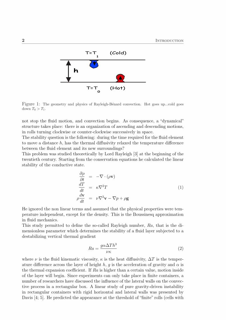
The origin of the term convection [1], from the Latin “convectio”, gives an ideaof “carrying with”. It seems to have been applied for the first time to denote thetransport of heat through fluid motion. Thermal convection arises when a thermalinhomogeneity exists in a fluid. This thermal inhomogeneity is a source of motionthrough different possible mechanisms, but stabilizing effects tend to dampen thesemotions. Generally, competition between these two opposite effects leads to an in-stability. The fundamental characteristic of such instabilities is the existence of athreshold beyond which there is organization of motion into a relatively orderedpattern.H. Benard [2] was the first person to study quantitatively the phenomenon of convec-tion in which instability is primarily due to temperature dependence of the surface-tension. In fact, it was at the turn of the last century that Benard reported oncarefully controlled experiments of convective motions in thin horizontal liquid lay-ers, where the lower surface was a metallic plate heated by steam and maintainedat a uniform temperature, while the upper surface was in free contact with air. Be-nard observed a first phase in which the fluid formed cells of almost regular shapes,nearly polygons of four to seven sides, which evolved to equal and regularly spacedhexagons.There is a different mechanism responsible for convection in which we are more in-terested in this thesis i.e. the Rayleigh-Benard convection [1], which has becomean experimental and theoretical paradigm for the study of systems out of the equi-librium. The Rayleigh-Benard experiment consists of a thin layer of fluid confinedbetween two horizontal, spatially-uniform, constant-temperature metal plates suchthat the bottom plate is maintained at a constant temperature higher than the up-per plate. The temperature difference generates a vertical gradient in the layer.The resulting stratification is formed by one denser layer located above another lessdense. This situation is clearly unstable.A fluid element located in the less dense region is not subjected to any upwardsforce, since its horizontal surroundings are of the same density. But, if we consider asmall ascending displacement of the fluid element, this will be surrounded by denserregions producing an buoyancy force that will sustain the initial displacement, towhich the thermal diffusivity and the viscous force will oppose. There is a thresh-old, due to the mechanism mentioned above, after which the dissipative effects can

1

2 Introduction

Figure 1: The geometry and physics of Rayleigh-Benard convection. Hot goes up...cold goesdown T0 > T1.

not stop the fluid motion, and convection begins. As consequence, a “dynamical”structure takes place: there is an organization of ascending and descending motions,in rolls turning clockwise or counter-clockwise successively in space.The stability question is the following: during the time required for the fluid elementto move a distance h, has the thermal diffusivity relaxed the temperature differencebetween the fluid element and its new surroundings?This problem was studied theoretically by Lord Rayleigh [3] at the beginning of thetwentieth century. Starting from the conservation equations he calculated the linearstability of the conductive state.

∂ρ

∂t= −∇ · (ρv)

dT

dt= κ∇2T (1)

ρdv

dt= ν∇2v −∇p + ρg

He ignored the non linear terms and assumed that the physical properties were tem-perature independent, except for the density. This is the Boussinesq approximationin fluid mechanics.This study permitted to define the so-called Rayleigh number, Ra, that is the di-mensionless parameter which determines the stability of a fluid layer subjected to adestabilizing vertical thermal gradient

Ra =gα∆Th3

νκ(2)

where ν is the fluid kinematic viscosity, κ is the heat diffusivity, ∆T is the temper-ature difference across the layer of height h, g is the acceleration of gravity and α isthe thermal expansion coefficient. If Ra is higher than a certain value, motion insideof the layer will begin. Since experiments can only take place in finite containers, anumber of researchers have discussed the influence of the lateral walls on the convec-tive process in a rectangular box. A linear study of pure gravity-driven instabilityin rectangular containers with rigid horizontal and lateral walls was presented byDavis [4; 5]. He predicted the appearance at the threshold of “finite” rolls (cells with

3

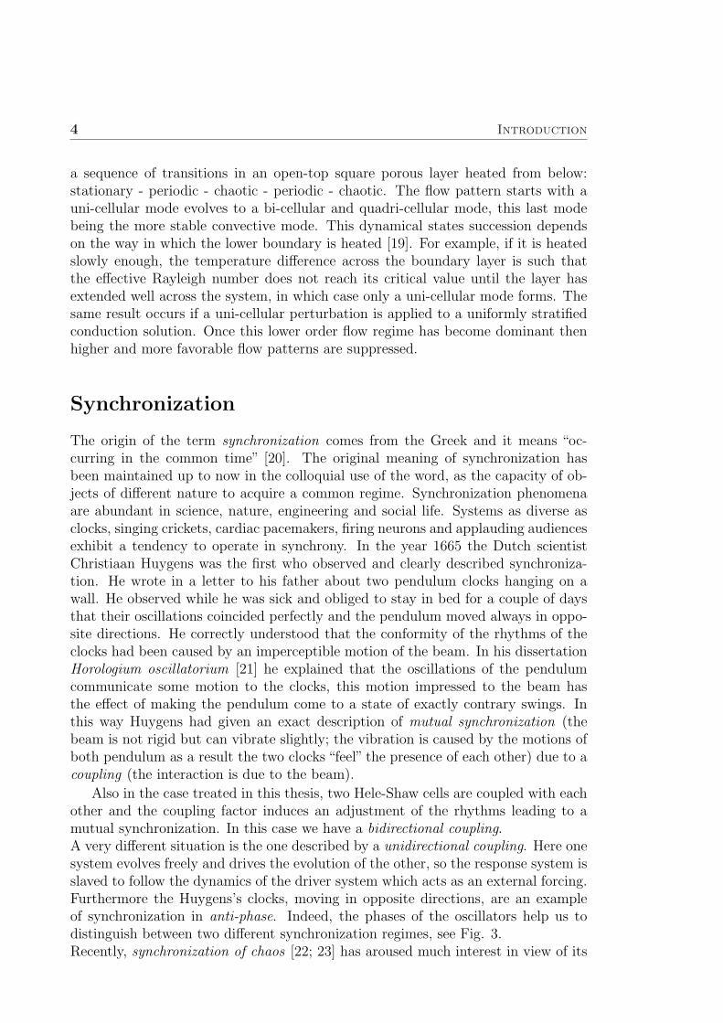
Figure 2: Convection in a porous media.

non-zero velocity components dependent on all three spatial variables) with axesparallel to the shorter side.The results on the onset of convection in rectangular vessels have been extendedto boxes of axisymmetric shape. Experiments in vessels of circular shape and largeextent have been performed by Koschmieder [6; 7] also by Koster and Muller [8] andalso more recently in smaller square boxes by Ondarcuhu et al. [9] and Ramon etal. [10].

Hele-Shaw and porous media

The Hele-Shaw cell was invented by British engineer Henry S. Hele Shaw before theturn of the twentieth century, and consists of two transparent plates separated bya small gap [11], so that one dimension is much smaller than the other two. It isvery useful because it reduces the complicated three dimensional flow of fluid to atwo dimensional flow. If the gap between the plates is sufficiently small the fluidflow between the plates held vertically and heated from below, is a good analog ofthe porous flow along ridge axes. For this reason, the governing equations for gap-averaged velocity components are identical with those for two-dimensional flow in aporous medium (the interested reader can see the detailed derivation in [12; 13]).As the Rayleigh number increases above a critical value of Rac = 4π2, the heat

transfer process changes from conduction to convection. This first transition has al-ready received considerable attention by Horton and Rogers (1945) [14] and Lapwood(1948) [15]. Their studies indicated that steady-state flow patterns evolved from aninitially motionless system and remained unchanged for all subsequent times. Itwas noticed later, that under certain conditions the flow became oscillatory. Theappearance of time dependent motion in a fluid layer uniformly heated from belowhas been suggested from Caltagirone et al. [16], and then Horne and O’Sullivan[17] who verified the existence of both stationary and oscillatory motions. Thereare more recent numerical works confirming the old results, where porous-mediaconvection for higher Rayleigh numbers has been treated with particular attentionas an illustration to the route to chaos. Cherkaoui and Wilcock [18] determined

4 Introduction

a sequence of transitions in an open-top square porous layer heated from below:stationary - periodic - chaotic - periodic - chaotic. The flow pattern starts with auni-cellular mode evolves to a bi-cellular and quadri-cellular mode, this last modebeing the more stable convective mode. This dynamical states succession dependson the way in which the lower boundary is heated [19]. For example, if it is heatedslowly enough, the temperature difference across the boundary layer is such thatthe effective Rayleigh number does not reach its critical value until the layer hasextended well across the system, in which case only a uni-cellular mode forms. Thesame result occurs if a uni-cellular perturbation is applied to a uniformly stratifiedconduction solution. Once this lower order flow regime has become dominant thenhigher and more favorable flow patterns are suppressed.

Synchronization

The origin of the term synchronization comes from the Greek and it means “oc-curring in the common time” [20]. The original meaning of synchronization hasbeen maintained up to now in the colloquial use of the word, as the capacity of ob-jects of different nature to acquire a common regime. Synchronization phenomenaare abundant in science, nature, engineering and social life. Systems as diverse asclocks, singing crickets, cardiac pacemakers, firing neurons and applauding audiencesexhibit a tendency to operate in synchrony. In the year 1665 the Dutch scientistChristiaan Huygens was the first who observed and clearly described synchroniza-tion. He wrote in a letter to his father about two pendulum clocks hanging on awall. He observed while he was sick and obliged to stay in bed for a couple of daysthat their oscillations coincided perfectly and the pendulum moved always in oppo-site directions. He correctly understood that the conformity of the rhythms of theclocks had been caused by an imperceptible motion of the beam. In his dissertationHorologium oscillatorium [21] he explained that the oscillations of the pendulumcommunicate some motion to the clocks, this motion impressed to the beam hasthe effect of making the pendulum come to a state of exactly contrary swings. Inthis way Huygens had given an exact description of mutual synchronization (thebeam is not rigid but can vibrate slightly; the vibration is caused by the motions ofboth pendulum as a result the two clocks “feel” the presence of each other) due to acoupling (the interaction is due to the beam).

Also in the case treated in this thesis, two Hele-Shaw cells are coupled with eachother and the coupling factor induces an adjustment of the rhythms leading to amutual synchronization. In this case we have a bidirectional coupling.A very different situation is the one described by a unidirectional coupling. Here onesystem evolves freely and drives the evolution of the other, so the response system isslaved to follow the dynamics of the driver system which acts as an external forcing.Furthermore the Huygens’s clocks, moving in opposite directions, are an exampleof synchronization in anti-phase. Indeed, the phases of the oscillators help us todistinguish between two different synchronization regimes, see Fig. 3.Recently, synchronization of chaos [22; 23] has aroused much interest in view of its

5

Figure 3: Possible synchronous regimes of two nearly identical oscillators. They may be synchro-nized in-phase, or in anti-phase.

potential applications. In particular, the use of chaotic synchronization in commu-nication systems has been investigated by several authors [24; 25]. A dynamicalsystem is called chaotic when its evolution is sensitive to small perturbations in itsinitial conditions [26]. This means that two close but different points in the phasespace will have trajectories that eventually separate exponentially. In other words,the evolution of a chaotic system cannot be predicted over a long time period.

The representation of a chaotic system in the phase space does not correspondto a simple geometrical object, but rather to a complex structure called strangeattractor.

Let us remember that a periodic oscillation is represented by a closed curve inthe phase space called limit cycle, see Fig. 4b. The origin of this term comes fromthe fact that the closed curve attracts all the trajectories from its neighborhood,which also explains the name simple attractor. The minimal dimension of the phasespace for a limit cycle oscillator is two, but this is not enough for chaotic motion totake place, since trajectories cannot intersect each other. A chaotic motion needsat least three dimensions. The Rossler model has exactly three dimensions and itsnumerical integration shows that this system lies on a strange attractor, see Fig. 4d.In the context of coupled chaotic systems many different synchronization states havebeen studied. In the present work, we have chosen to use strong coupling in orderto make the states of both oscillators identical. As a result, the signals coincideand we obtain a regime of complete synchronization. But, we have to pay attentionto how strong is the coupling, for example, if we consider two oscillators that aremechanically coupled with a rigid link, we can not speak of synchronization becausethe coupling imposes too strong limitations on the motion of the two systems. Todetermine what can be considered as a weak or a strong coupling is rather difficult,but we can say that the introduction of coupling should not qualitatively changethe behavior of the interacting systems. The motion of the attractor exhibits thesensitive dependence on initial conditions. As mentioned before this means thattwo trajectories starting very close together will rapidly diverge from each other,and thereafter have totally different futures. The growth rate is called Lyapunovexponent. Consider the trajectories x(k) and y(k), starting, respectively, from x(0)and y(0). If both trajectories are, until time k, always in the same linear region, wecan write

|x(j + 1)− y(j + 1)| = |f ′(x(j))||x(j)− y(j)|, j = 0, 1, ..., k − 1 (3)

6 Introduction

a) b)

0 0.02 0.04 0.06 0.08

time

10.4

10.6

10.8

11

11.2

x

10.4 10.6 10.8 11 11.2

x

0.35

0.355

0.36

0.365

y

c) d)

0 50 100 150

time

−20

−10

0

10

20

x

−20 −10 0 10 20

x

−20

−10

0

10

20

y

Figure 4: a) and b) Periodic oscillation is represented by a closed curve in the phase space. c)The Rossler’s attractor. d) For the variables x, y the dynamics of the Rossler model look likerotations around the center, with irregular amplitude and an irregular return time.

where f ′(x) denotes the derivative of f at x. Thus,

|x(k)− y(k)| = |f ′(x(k − 1))||f ′(x(k − 2))| . . . |f ′(x(0))||x(0)− y(0)| (4)

or equivalently

|x(k)− y(k)| = eλk|x(0)− y(0)| (5)

where

λ =1

k

k−1∑j=0

ln|f ′(x(j))|. (6)

The equation (6) defines the Lyapunov exponent of the trajectory x(k).The interpretation of (5) is that λ gives the average rate of divergence (if λ > 0),or convergence (if λ < 0) of the two trajectories from each other, during the timeinterval [0, k].

The scope of this work

The first objective of the present study is to calculate the evolution of the flow andheat transport patterns in a Hele-Shaw cell uniformly heated from below, from theonset of convection to relatively high Rayleigh numbers (Ra ' 30Rac). Having foundthe Rayleigh number’s value from which the chaotic regime begins (Ra = 1100), themain purpose is to achieve the synchronization between two identical Hele-Shaw

7

cells laying in the chaotic regime.

A mathematical formulation of the modeling of the flow in a Hele-Shaw cell isproposed in Chapter 1. The configuration, which we have modeled consists in a boxof porous material heated uniformly from below. It is a bounded two-dimensionalsquare porous layer of thickness (height) h. The vertical boundaries are consideredadiabatic. The horizontal top and bottom are isothermal, with the bottom warmerthan the top, see Fig. 2. When no motion occurs, a vertical linear temperaturedistribution is set in the system.The Chapters 2 and 3 are dedicated to explain the different numerical proceduresthat can be used to calculate the evolution of the temperature and velocity in thebox. In order to integrate the flow during a long period in time, we propose a set ofnumerical methods, which permit to compute in an accurate and stable way the timeevolution of the system. In chapter 2 we discuss the discretization of initial-valueproblems, considering, more specifically the advection-diffusion equations. One-stepand multistep methods are considered for explicit and implicit schemes, paying spe-cial attention to the accuracy and stability of discretization. Chapter 3 is devoted tosolve boundary value problems, essentially the Poisson, or more generally, Helmholtzequations. Also, in this case we offer different methods to find solutions in a rapidway, underlaying the success of the Fourier transform algorithms (FFT).In chapter 4, we describe the results of the numerical integrations. We give theRayleigh numbers that separate the different dynamical regimes. We describe thecharacteristics of the convective patterns after each transition, and analyze theireffects on the heat transport through the analysis of the Nusselt number.In the last chapter, after a brief discussion over what determines the spatial struc-tures of the flow, we investigate possible synchronization mechanisms between twoHele-Shaw cells. Using a weak bidirectional thermal coupling between all the pointsof the two systems, we obtain the complete coincidence of the states. We also inves-tigate the minimal number of points necessary to get synchronization and also thepossibility of coupling both systems only through the lateral walls.

Chapter 1

Mathematical Formulation

1.1 Governing equations

A porous medium is a material consisting of a solid matrix with an interconnectedvoid [12; 13]. The interconnectedness of the void (the pores) allows the flow of oneor more fluids through the material.In a natural porous medium the distribution of pores with respect to shape andsize is irregular. On the pore scale (the microscopic scale) the flow quantities willbe irregular, but many of these quantities are measured over areas that cross manypores, and such space-averaged (macroscopic) quantities change in a regular mannerwith respect to space and time.The usual way of deriving the laws governing the macroscopic variables is to beginwith the standard equations obeyed by the fluid [27; 28] and to obtain the macro-scopic equations by averaging over volumes or areas containing many pores. Inthe textbook “Convection in Porous Media” [13] the authors construct a continuummodel for a porous medium using a spatial approach: a macroscopic variable is de-fined over a sufficiently large representative elementary volume (r.e.v.). The valueof the variable is evaluated in center of the volume and it is assumed that the resultis independent of the size of the r.e.v.In our problem, we will consider a bounded two-dimensional square porous layer ofthickness h. The vertical boundaries are adiabatic. The horizontal boundaries areisothermal. The temperature difference across the porous layer is ∆T = T0 − T1,the porous layer is heated from below. Let us briefly recall what are the governingequations for such system:Conservation of mass.The expression for the continuity equation for a flow through porous media is givenby:

φ∂ρf

∂t+∇ · (ρfv) = 0, (1.1)

where ρf is the fluid density, v is the fluid velocity and φ is the porosity of theporous medium, defined as the fraction of the total volume of the medium that isoccupied by void space.Conservation of momentum.

9

10 chapter 1. Mathematical Formulation

The usual Navier-Stokes equation is replaced by the Darcy’s law which is assumedto describe the flow. The Darcy’s law expresses proportionality between the flowrate and the applied pressure difference:

∇p = −µ

kv, (1.2)

where ∇p is the pressure gradient in the flow direction, µ is the dynamic viscosityof the fluid and k is the permeability of the medium.An extension of the equation (1.2) for the conservation of the momentum can beexpressed in the following way:

ρf

(φ−1∂v

∂t+ φ−2(v · ∇)v

)= ρfg −∇p− µ

kv, (1.3)

where g is the acceleration due to gravity [12].Conservation of energy.

(φ(ρc)f + (1− φ)(ρc)s)∂T

∂t+ (ρc)fv · ∇T = λ∇2T, (1.4)

where (ρc)s and (ρc)f are respectively the heat capacity of the solid material and ofthe fluid and λ is the thermal conductivity of the fluid-saturated porous medium.Since φ is small for most relevant systems, the energy equation can be reduced to

σ∂T

∂t+ v · ∇T = κ∇2T, (1.5)

where σ = (ρc)s/(ρc)f is typically near unity and κ is the thermal diffusivity of thefluid-saturated porous medium. In the following we will assume σ = 1.

For thermal convection to occur, the density of the fluid must be a function ofthe temperature, hence we need an equation of state to complement the equationsof mass, momentum and energy. The simplest equation of state is:

ρf = ρ0[1− α(T − T0)], (1.6)

where ρ0 is the fluid density at some reference temperature T0 and the positive con-stant α is the thermal expansion coefficient. Equation (1.6) is obtained from thefirst term of the Taylor expansion of the equation of state of ρ = ρ(p, T ) in whichthe pressure variations are neglected.It is usual in convection problems to invoke the Boussinesq’s approximation. Thisconsists of setting constant all properties of the medium, except the one that in-volves the buoyancy term, hence α is retained in the momentum equation. As aconsequence the equation of continuity reduces to ∇ · v = 0. The Boussinesq’sapproximation is valid as long as that density changes remain small in comparisonwith ρ0, and provided that the temperature variations are insufficient to vary theproperties of the medium from their mean values.Also the momentum equation may be simplified further by comparing the relativemagnitude of the separate terms. Using this argument the equation (1.3) reduces to

v =k

µ(−∇p + ρfg). (1.7)

Section 1.1. Governing equations 11

1.1.1 Stream function equation reformulation

As an alternative way of solving the governing equations in primitive variables, itis also possible to avoid the explicit appearance of the pressure by using the streamfunction formulation.In two dimensions the governing equations are:

∂u

∂x+

∂v

∂y= 0, (1.8)

∂p

∂x+

µ

ku = 0, (1.9)

ρ0[1− α(T − T0)]g +∂p

∂y+

µ

kv = 0, (1.10)

∂T

∂t+ u

∂T

∂x+ v

∂T

∂y= κ

(∂2T

∂x2+

∂2T

∂y2

). (1.11)

In order to remove the pressure variable, we derive equation (1.10) with respect tox and subtract the derivative of equation (1.9) with respect to y. The resultingequation is:

−αρ0g∂T

∂x+

µ

k

(∂v

∂x− ∂u

∂y

)= 0. (1.12)

In two dimensions the stream function is defined by:

u =∂ψ

∂y; v = −∂ψ

∂x. (1.13)

Using the stream-function formulation the equations become:

∇2ψ = −αgkρ0

µ

∂T

∂x,

∂T

∂t+

∂ψ

∂y

∂T

∂x− ∂ψ

∂x

∂T

∂y= κ

(∂2T

∂x2+

∂2T

∂y2

). (1.14)

The equations may now be expressed in dimensionless form, by introducing thenew dimensionless variables:

t =h2

κt

x =x

h

u =h

κu

ψ =ψ

κ

T =T

T1 − T0

=T

∆T(1.15)

12 chapter 1. Mathematical Formulation

after which the equations become:

∂T

∂t= ∇2T +

∂ψ

∂y

∂T

∂x− ∂ψ

∂x

∂T

∂y,

∇2ψ = −Ra∂T

∂x, (1.16)

where Ra is the Rayleigh number and is defined by:

Ra =αgkρ0h∆T

µκ, (1.17)

this number is a dimensionless parameter that measures the applied temperaturedifference. For an infinitely horizontally extended porous medium, the linear the-ory gives a Rayleigh number equals at the onset of convection to 4π2 (Lapwood [15]).

In this thesis, we have considered isothermal conditions at the lower and at theupper boundaries:

T (x, 0) = T0 = 1 T (x, 1) = T1 = 0, (1.18)

and adiabatic conditions at the lateral walls:

∂T

∂x(0, y) =

∂T

∂x(1, y) = 0. (1.19)

The stream-function vanishes at all boundaries as a result of the impermeability ofthe walls. In the following, in order to make the notation lighter, tildes are omittedbut all variables are dimensionless.

1.1.2 The Nusselt number

An important consequence of convective motions is the increase of the heat flux qthrough the layer. Below the onset of convection ∆T < ∆Tc, and q is only due toconduction, q = qcond. In contrast, when the fluid motion is present, the fluid velocityentails a supplementary heat flux qconv, and then the total heat flux q = qcond + qconv

is higher than it would be in a purely conductive state.This is expressed by the Nusselt number:

Nu =qcond + qconv

qcond

. (1.20)

Hence Nu = 1 provided that Ra < Rac. For Ra > Rac the Nusselt number increasesreflecting the increasing part of the convection in the heat transport.For a layer internally heated from below:

Nu = −∫ 1

0

∂T

∂y|y=0dx. (1.21)

It can be easily checked, by substitution of the linear temperature profile in (1.21),that the reference value is given by Nu = 1 (for conduction).

Chapter 2

Solutions of Diffusive Initial ValueProblems

Rayleigh-Benard convection is so important that many numerical methods havebeen developed and tried over the years although [29; 30], somewhat unfortunately,most of these methods have not been compared with each other to determine whichbest achieves a practical balance of efficiency, accuracy, ease of programming, andparallel scalability on some specific computer architecture. Because our interest isto study fundamental questions in simple cell geometries, we chose not to use finiteelement [31; 32] or spectral methods [33; 34; 35] whose main strengths are the abilityto handle irregular boundaries. In the present thesis, we have chosen second orderaccurate finite difference approximations.

2.1 Grid based methods and simple finite differ-

ences

The basic idea of a finite difference procedure [36; 37; 38] is to replace the continuousproblem domain with a finite-difference mesh containing a finite number of gridpoints. In order to represent a function f on a two-dimensional domain spannedby Cartesian coordinates (x, y), we use f(j∆x, i∆y). The grid points are locatedaccording to values of i and j, so difference equations are usually written in termsof the general point (j, i) and its neighbors.The standard approach for approximating the differentials comes from truncatedTaylors series [39; 40]. Consider a function f(x, t) at a fixed time t. If f is sufficientlycontinuous in space we can expand it around any point f(x + ∆x) as

f(x + ∆x) = f(x) + ∆x∂f

∂x(x) +

(∆x)2

2

∂2f

∂x2(x) + ...

+(∆x)n−1

(n− 1)!

∂n−1f

∂xn−1(x) +

(∆x)n

n!

∂nf

∂xn(ξ) x ≤ ξ ≤ x + ∆x (2.1)

13

14 chapter 2. Solutions of Diffusive Initial Value Problems

where the last term can be identified as the remainder. If we ignore in this seriesterms of order ∆x2 and higher, we could approximate the first derivative at anypoint x0 as

∂f

∂x(x0) ≈ f(x0 + ∆x)− f(x0)

∆x+ O(∆x) (2.2)

where the last term is called the truncation error and it is the difference betweenthe actual partial derivative and its finite-difference representation.If we consider that our function is now stored in a discrete array of points fj andx = j∆x where ∆x is the grid spacing, then at time step n we can write

∂f

∂x(x0) ≈

fnj+1 − fn

j

∆x+ O(∆x) (2.3)

where (fnj+1 − fn

j )/∆x is the finite difference representation for (∂f/∂x)j.An identical procedure but expanding in time gives

∂f

∂t(t0) ≈

fn+1j − fn

j

∆t+ O(∆t) (2.4)

Both of these approximations are however first order accurate as the leading termin the truncation error is of order ∆x or ∆t.

Figure 2.1: Forward space step.

2.1.1 Higher order finite difference schemes

In equation (2.1), we have considered the value of our function at one point forwardin ∆x. We could just have easily taken a step backward to get

f(x−∆x) = f(x)−∆x∂f

∂x(x0) +

(∆x)2

2

∂2f

∂x2(x0) + O(∆x3) (2.5)

If we truncate at order ∆x2 and above we still get a first order approximation

∂f

∂x(x0) ≈

fnj − fn

j−1

∆x+ O(∆x) (2.6)

which is not any better than the forward step as it has the same order error (but ofopposite sign). An improved scheme is obtained by combining equation (2.1) and(2.5) to remove the equal but opposite second order terms. If one subtracts (2.5)from (2.1) one gets the centered space approximation

∂f

∂x(x0) ≈

fnj+1 − fn

j−1

2∆x+ O(∆x2) (2.7)

Section 2.1. Grid based methods and simple finite differences 15

Figure 2.2: Backward and centered space step.

Note that we have still two grid points to approximate the derivative but we havegained an order of magnitude in the truncation error. By including more and moreneighboring points, even higher order schemes can be obtained.After considering the first derivative, we have also to consider an approximation forthe second derivative. This time by adding (2.1) and (2.5) and rearranging we get

∂2f

∂x2(x0) ≈

fnj+1 − 2fn

j + fnj−1

(∆x)2+ O(∆x2) (2.8)

This approximation only requires a point and its two neighbors.

2.1.2 Multi-dimensions

What we have done in one dimension in the first section, we generalize it to multi-dimension. Consider, for example, a function f(x, y, t) at fixed time t and fixed pointy. If f is continuous in space we can expand it again around any point f(x+∆x, y)or f(x, y + ∆y). So if we ignore terms of order ∆x2 and ∆y2, and higher, and storethe function in a discrete matrix of points fi,j where x = j∆x and y = i∆y are thegrid spacings, at time steps n, we can write

∂f

∂x(x0, y0) ≈

fni,j+1 − fn

i,j−1

2∆x+ O(∆x2) (2.9)

or∂f

∂y(x0, y0) ≈

fni+1,j − fn

i−1,j

2∆y+ O(∆y2) (2.10)

at any point (x0, y0). In the same way, we can obtain an approximation for thesecond derivatives

∂2f

∂x2(x0, y0) ≈

fni,j+1 − 2fn

i,j + fni,j−1

(∆x)2+ O(∆x2) (2.11)

or for example

∂2f

∂x∂y(x0, y0) ≈

fni+1,j+1 − fn

i−1,j+1 − fni+1,j−1 + fn

i−1,j−1

4∆x∆y+ O(∆x2) + O(∆y2) (2.12)

16 chapter 2. Solutions of Diffusive Initial Value Problems

Figure 2.3: The second derivatives at the point A are evaluated using the points to which A isshown connected. The second derivatives at the point B are evaluated using the connected pointsand also using ”right-hand-side” boundary information, as shown schematically.

2.2 Numerical solutions of the diffusion equation

Let us consider the two-dimensional diffusion equation:

∂T

∂t= ∇2T. (2.13)

We will begin considering how to solve the diffusion equation numerically by derivingsome finite difference approximations to the Laplacian term [29; 38; 41; 42]. Givena 2-D square grid, we will use i and j to number the grid lines in the y and the xdirections, respectively, with i, j = 0, ..., N and ∆y = ∆x = ∆.Accordingly with last section, we represent the Laplacian as

∇2T =Ti+1,j − 2Ti,j + Ti−1,j

∆2+

Ti,j+1 − 2Ti,j + Ti,j−1

∆2(2.14)

which is a second-order accurate approximation.For convenience and future notation, it is useful to write (2.14) as

∇2T =1

∆x2

11 −2 1

1

Ti,j +

1

∆y2

11 −2 1

1

Ti,j (2.15)

which is an operator that acts on a point T (i, j) and its two nearest neighbors and itis represented by a tridiagonal matrix that is primarily zero except for the diagonal(which has value −2) and the super- and sub-diagonal (of value 1).Given a discretization of the thermal diffusion term we still need to add the timederivative for the left-hand-side. Using a forward time step the approximation ofthe diffusion equation can be written

T n+1i,j − T n

i,j

∆t=

T ni+1,j − 2T n

i,j + T ni−1,j

∆2+

T ni,j+1 − 2T n

i,j + T ni,j−1

∆2(2.16)

Section 2.2. Numerical solutions of the diffusion equation 17

or, in matrix form

T n+1i,j − T n

i,j

∆t=

1

∆2

11 −4 1

1

T n

i,j

T n+1i,j = T n

i,j + α

11 −4 1

1

T n

i,j

T n+1i,j =

αα 1− 4α α

α

T n

i,j (2.17)

where

α =∆t

∆2(2.18)

physically corresponds to the number of grid points that heat reaches in a time step(or it is the inverse of the number of time step required for heat to diffuse a gridspace) [43; 44].

2.2.1 Stability analysis

From the material presented thus far, it is evident that a variety of numerical schemescan be written, but they are not all equally acceptable. The difference representationgiven by (2.16) is referred to as the simple explicit scheme for the heat diffusionequation (Euler scheme). An explicit scheme is one for which only one unknownappears in the difference equation in a manner that permits evaluation in terms ofknown quantities.The first requirement that any scheme should meet is that of stability. A stablescheme is defined as one for which errors from any source are not permitted to growin the sequence of numerical procedures as the calculation proceeds from one stepto the next.The Von Neumann stability analysis is perhaps the most widely used for establishingthe stability characteristics of a finite-difference scheme. Instead of considering thebehavior of the truncated terms we will now consider the behavior of small sinusoidalerrors. If S is the exact solution of the difference scheme, we suppose to haveobtained S + δ, where δ is the results of errors arising from any sources. If wesubstitute in the equation (2.16), S will cancel out because it satisfies the differenceequation, we have

δn+1i,j − δn

i,j

∆t=

δi+1,j − 2δi,j + δi−1,j

∆2+

δi,j+1 − 2δi,j + δi,j−1

∆2. (2.19)

If the difference equation is linear, the errors will satisfy an equation of the sameform as the original difference equation.

18 chapter 2. Solutions of Diffusive Initial Value Problems

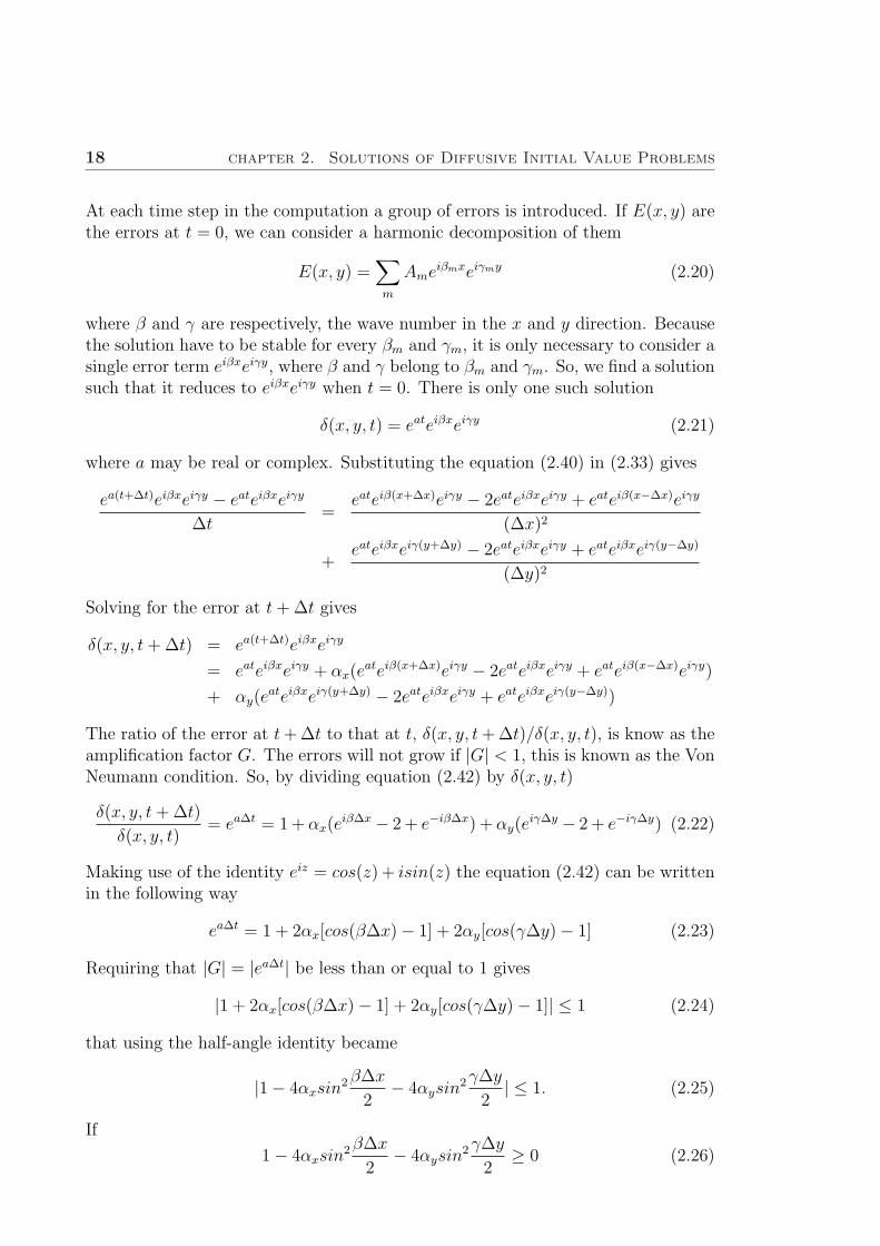
At each time step in the computation a group of errors is introduced. If E(x, y) arethe errors at t = 0, we can consider a harmonic decomposition of them

E(x, y) =∑m

Ameiβmxeiγmy (2.20)

where β and γ are respectively, the wave number in the x and y direction. Becausethe solution have to be stable for every βm and γm, it is only necessary to consider asingle error term eiβxeiγy, where β and γ belong to βm and γm. So, we find a solutionsuch that it reduces to eiβxeiγy when t = 0. There is only one such solution

δ(x, y, t) = eateiβxeiγy (2.21)

where a may be real or complex. Substituting the equation (2.40) in (2.33) gives

ea(t+∆t)eiβxeiγy − eateiβxeiγy

∆t=

eateiβ(x+∆x)eiγy − 2eateiβxeiγy + eateiβ(x−∆x)eiγy

(∆x)2

+eateiβxeiγ(y+∆y) − 2eateiβxeiγy + eateiβxeiγ(y−∆y)

(∆y)2

Solving for the error at t + ∆t gives

δ(x, y, t + ∆t) = ea(t+∆t)eiβxeiγy

= eateiβxeiγy + αx(eateiβ(x+∆x)eiγy − 2eateiβxeiγy + eateiβ(x−∆x)eiγy)

+ αy(eateiβxeiγ(y+∆y) − 2eateiβxeiγy + eateiβxeiγ(y−∆y))

The ratio of the error at t + ∆t to that at t, δ(x, y, t + ∆t)/δ(x, y, t), is know as theamplification factor G. The errors will not grow if |G| < 1, this is known as the VonNeumann condition. So, by dividing equation (2.42) by δ(x, y, t)

δ(x, y, t + ∆t)

δ(x, y, t)= ea∆t = 1 + αx(e

iβ∆x − 2 + e−iβ∆x) + αy(eiγ∆y − 2 + e−iγ∆y) (2.22)

Making use of the identity eiz = cos(z) + isin(z) the equation (2.42) can be writtenin the following way

ea∆t = 1 + 2αx[cos(β∆x)− 1] + 2αy[cos(γ∆y)− 1] (2.23)

Requiring that |G| = |ea∆t| be less than or equal to 1 gives

|1 + 2αx[cos(β∆x)− 1] + 2αy[cos(γ∆y)− 1]| ≤ 1 (2.24)

that using the half-angle identity became

|1− 4αxsin2β∆x

2− 4αysin

2γ∆y

2| ≤ 1. (2.25)

If

1− 4αxsin2β∆x

2− 4αysin

2γ∆y

2≥ 0 (2.26)

Section 2.3. Implicit scheme and stability:Crank-Nicholson scheme 19

that is

−4αxsin2β∆x

2− 4αysin

2γ∆y

2≤ 0 (2.27)

the inequality is always satisfied because α > 0. Whereas if

1− 4αxsin2β∆x

2− 4αysin

2γ∆y

2< 0 (2.28)

that is

αxsin2β∆x

2+ αysin

2γ∆y

2≤ 1

2(2.29)

the inequality is satisfied if

αx + αy ≤ 1

2. (2.30)

If ∆x = ∆y the condition (2.30) becomes

2α ≤ 1

2. (2.31)

This provides the stability requirement for this method. This means that a decreasein grid spacing, for example, by a factor of 2 in both direction requires a factor of16 more computer time. In fact, this choice for ∆x implies that the grid’s pointnumbers is increased by a factor 4 and from the condition (2.31) it follows that thenew ∆t is four times smaller than the original time step. Unfortunately, because thesimplest centered schemes are only second order in space (and first order in time), wegain only a factor of 4 in reducing the truncation error. Fortunately, this is not theonly scheme available. We will develop implicit schemes which are unconditionallystable and we will can take as large a step as we want.

2.3 Implicit scheme and stability:

Crank-Nicholson scheme

At the end of the last section we have shown that if we use an explicit scheme wehave to choose time steps that satisfy the restriction (2.31). But, sometimes timesteps comparable to, or smaller than, (∆x)2/4 may be physically unreasonable. Forthis reason we will use a implicit scheme which is unconditionally stable.In an explicit scheme we have only one unknown, since the parabolic heat equationgoverns a marching problem for which an initial distribution of T must be specified.The temperature field T at time level n can be considered to be known. If thesecond derivative term in the heat equation were approximated by the temperaturefield taken at the n + 1 time level, three unknowns would appear in the differenceequation. In this case the procedure is called implicit, indicating that the algebraicformulation would require the simultaneous solution of several equations involvingthe unknowns.The simplest implicit scheme for the heat diffusion equation can be developed fromthe Taylor series by simply evaluating the heat diffusion term at the n+1 time level

20 chapter 2. Solutions of Diffusive Initial Value Problems

(all we have to do is to rewrite equation (2.16) replacing the diffusion rate at timestep n with that at time step n + 1):

T n+1i,j − T n

i,j

∆t=

T n+1i+1,j − 2T n+1

i,j + T n+1i−1,j

∆2+

T n+1i,j+1 − 2T n+1

i,j + T n+1i,j−1

∆2(2.32)

or, in matrix form

T n+1i,j = T n

i,j + α

11 −4 1

1

T n+1

i,j . (2.33)

This is an implicit method because we do not know in advance what the right-hand-side will evaluate to, however, we can again rearrange (2.33) to solve T n+1

i,j

as

T ni,j =

−α−α 1 + 4α −α

−α

T n+1

i,j (2.34)

This scheme is first order accurate in time and second order accurate in space.The Von Neumann method can easily be applied to this scheme to determine itsstability characteristics. Proceeding in the same way that for the explicit scheme,we obtain that the error satisfy an equation of the same form as equation (2.32).Substituting δ(x, y, t) = eateiβxeiγy into that equation and requiring that |G| ≤ 1gives

|G| =(

1 + 4αsin2β∆x

2+ 4αsin2γ∆y

2

)−1

≤ 1 (2.35)

which is satisfied for any α ≥ 0. So, the difference equation is effectively, uncondi-tionally stable.We can obtain a second order scheme in both space and time, simply averaging theexplicit and implicit schemes:

T n+1i,j − T n

i,j

∆t=

1

2

((T n+1

i+1,j − 2T n+1i,j + T n+1

i−1,j) + (T ni+1,j − 2T n

i,j + T ni−1,j)

∆2

)

+1

2

((T n+1

i,j+1 − 2T n+1i,j + T n+1

i,j−1) + (T ni,j+1 − 2T n

i,j + T ni,j−1)

∆2

)(2.36)

Here both the left- and the right-hand sides are centered at time step n+1/2, so themethod is second-order accurate in time, as we said. This scheme is called Crank-Nicholson scheme and it is also unconditionally stable.Inspection of (2.36), shows that Crank-Nicholson in one dimension is a system oflinear equations of the form

Ax = b (2.37)

where A is a tridiagonal matrix that is primarily zero except for the diagonal (whichhas value (1 + 4α)) and one super and sub diagonal (of value −α). For (2.37) the

Section 2.3. Implicit scheme and stability:Crank-Nicholson scheme 21

vector x corresponds to the matrix of the temperature values at the time step n+1,Tn+1, and the vector b is the known temperature at time n. So, we want solve

ATn+1 = Tn (2.38)

A is a symmetric and positive definite matrix, so it can be inverted. Tridiagonalmatrix can be inverted in order N operations where N is the total number of gridpoints. The IMSL library provides efficient implementations of tridiagonal solversand shows that tridiagonal algorithm makes the implicit methods very competitivefor the heat diffusion equation in terms of computational effort.Unfortunately in two dimensions this scheme is no longer tridiagonal. In fact theextension of the Crank-Nicholson scheme (to two dimensions) leads to a system oflinear equations that contains five unknowns for two dimensions. It looks like

−1−1 2(2 + α) −1

−1

T n+1 =

11 2(2− α) 1

1

T n (2.39)

equation (2.39) is a “band” tridiagonal system of simultaneous linear equations andthe inversion of the matrix in this case is significant more expensive computationally.However the scheme remains unconditionally stable. One possibility to solve themis use a sparse matrix technique, or another approach, which combines second orderaccuracy in space and time with the ease of tridiagonal solvers, is the Alternating-Direction Implicit scheme.

2.3.1 Alternating-Direction Implicit scheme

One possibility is to use the ADI scheme, the idea is split one process into its dif-ferent directional components. For example, we could rewrite our multidimensionaldiffusion equation as

∂T

∂t= LxT + LyT (2.40)

where Lx is the operator controlling diffusion in the horizontal direction and Ly

controls diffusion in the vertical direction. Given this splitting, ADI schemes thensolve (2.40) by taking two-passes, first solving an implicit diffusion equation in thehorizontal for the first half time step and then an implicit diffusion equation in thevertical for the second half time step.In more detail, the ADI algorithm for (2.13) looks like

Tn+ 1

2i,j − T n

i,j

∆t/2=

1

∆x2

(T

n+ 12

i+1,j − 2Tn+ 1

2i,j + T

n+ 12

i−1,j

)

+1

∆y2

(T n

i,j+1 − 2T ni,j + T n

i,j−1

)(2.41)

T n+1i,j − T

n+ 12

i,j

∆t/2=

1

∆x2

(T

n+ 12

i+1,j − 2Tn+ 1

2i,j + T

n+ 12

i−1,j

)

+1

∆y2

(T n+1

i,j+1 − 2T n+1i,j + T n+1

i,j−1

)(2.42)

22 chapter 2. Solutions of Diffusive Initial Value Problems

Only one tridiagonal system of equations must be solved for each half step. Theequation (2.42) is an implicit, tridiagonal equation for the horizontal rows at timen+1/2 which are then used in the equation (2.42) to update the vertical columns attime n+1. The tridiagonal nature of these two schemes can be made more apparentif we collect terms of the same time step together. For a uniform grid we can rewritethe equations (2.42) as

[−1 α + 2 − 1]T n+ 12 =

1α− 2

1

T n

−1α + 2−1

T n+1 = [1 α− 2 1]T n+ 1

2 (2.43)

where a horizontal stencil implies horizontal neighbors and vertical stencil impliesvertical neighbor.The advantage of this method is that each time step requires only the solution oftwo simple tridiagonal systems.

2.4 The non-linear term

Our diffusion equation is not linear, it has the following form

∂T

∂t= ∇2T + J, (2.44)

where J is the Jacobian non linear term and in two dimensions it is written

J =∂ψ

∂y

∂T

∂x− ∂ψ

∂x

∂T

∂y(2.45)

this term is also known as the advection term. By studying the way to constructa computer model of the general circulation of the atmosphere, Arakawa [45] hasexplained that a simple finite difference approximation using central differences, forexample

∂ψ

∂y

∂T

∂x=

(ψi+1,j − ψi−1,j) (Ti,j+1 − Ti,j−1)

4∆2(2.46)

causes numerical instability. At first he thought his problems were “truncation er-ror”. A computer cannot produce numbers with infinite precision. When thousandsof calculation are repeated and the numbers are truncated each time, we add uptiny discrepancies over and over. As result we have a big discrepancy. Eventuallythe solutions became unrealistic and “explode”. But after that Arakawa recognizedthat the instability was like the problem of a platoon of soldiers ordered to marchacross a bridge. If they march across in step, it may happen that somewhere there isa combination that resonates at just the frequency of their marching. Each time thefeet come down, they hit that combination at the same phase of its swing, pushing

Section 2.4. The non-linear term 23

it a little further. Soldiers know that bridges can resonate and they will break stepbefore crossing.Something like this happened with Arakawa’s simulations. Suppose the computergoes through a complete step and takes its next step after a simulation interval of,for example, one hour. Among the simulated waves there would be some with afrequency of just one hour. Every time the calculation was repeated, the computerwould catch those waves at the same phase (aliasing occurs when the sampling fre-quency is too low with respect to the frequency content in the original time series.A new, but false frequency is obtained by the sampling procedure). Arakawa soughta way to make the small pushes cancel one another out, as the impact of the feetof the soldiers would cancel one another if they broke step. The key, he found, wasto write equations in such a way that certain quantities would remain unchanged.For example, the kinetic energy. In the real world, the law of conservation of energydemands that there is never any change in the total energy, whereas kinetic energyalone is not normally conserved. But by using equations that did conserve kineticenergy, Arakawa could make sure that no unrealistic spike of wind speed grew ex-ponentially from his calculations.To avoid aliasing errors Arakawa developed nine- and thirteen-point representationsof the Jacobian J which conserve the kinetic energy and which have a truncationerror of the square and fourth power, respectively, of the spatial difference x. Thesenumerical schemes are known as the second and fourth-order Arakawa schemes.We choose second order Arakawa scheme. There are different possibilities to writethe expression for the Jacobian [46; 47]:

J(ψ, T ) =∂ψ

∂y

∂T

∂x− ∂ψ

∂x

∂T

∂y

=∂

∂x

(ψ

∂T

∂y

)− ∂

∂y

(ψ

∂T

∂x

)

=∂

∂y

(T

∂ψ

∂x

)− ∂

∂x

(T

∂ψ

∂y

)

=1

2r

{(∂ψ

∂y− r

∂ψ

∂x

)(∂T

∂y+ r

∂T

∂x

)−

(∂T

∂y− r

∂T

∂x

)(∂ψ

∂y+ r

∂ψ

∂x

)}

The last expression follows from

η = x− y

r

ξ = x +y

r

from which

∂

∂η=

1

2

(∂

∂x− r

∂

∂y

),

∂

∂ξ=

1

2

(∂

∂x+ r

∂

∂y

), (2.47)

24 chapter 2. Solutions of Diffusive Initial Value Problems

and

J(ψ, T ) =2

r

{∂ψ

∂y

∂T

∂x− ∂ψ

∂x

∂T

∂y

}(2.48)

The resulting schemes will depend on the choice of the mathematical expression forthe Jacobian. From the first expression we have

J++ =1

4∆x∆y

{(ψi,j+1−ψi,j−1)(Ti+1,j − Ti−1,j)− (ψi+1,j −ψi−1,j)(Ti,j+1− Ti,j−1)

},

from the second expression we get:

J+× =1

4∆x∆y

{ψi,j+1(Ti+1,j+1 − Ti−1,j+1)− ψi,j−1(Ti+1,j−1 − Ti−1,j−1)

− ψi+1,j(Ti+1,j+1 − Ti+1,j−1) + ψi−1,j(Ti−1,j+1 − Ti−1,j−1)

}, (2.49)

the third one leads to:

J×+ =1

4∆x∆y

{Ti+1,j(ψi+1,j+1 − ψi+1,j−1)− Ti−1,j(ψi−1,j+1 − ψi−1,j−1)

− Ti,j+1(ψi+1,j+1 − ψi−1,j+1) + Ti,j−1(ψi+1,j−1 − ψi−1,j−1)

}, (2.50)

finally, from the last one with r = ∆y/∆x:

J×× =1

8∆x∆y

{(ψi−1,j+1 − ψi+1,j−1)(Ti+1,j+1 − Ti−1,j−1)

− (ψi+1,j+1 − ψi−1,j−1)(Ti−1,j+1 − Ti+1,j−1)

}. (2.51)

A viable form to represent the Jacobian is

J = aJ++ + bJ×+ + cJ+× + dJ××, a + b + c + d = 1 (2.52)

In the discretized expression for the Jacobian J the two super-indices indicate thepoints where ψ and T are evaluated respectively. For example, J+× means that ψis evaluated in the adjacent horizontal and vertical points and T is evaluated withthe neighboring points on the diagonals. In the present thesis, we have chosen touse d = 0 and a = b = c = 1/3 for the discretization of the Jacobian [17].

2.5 Multistep methods

The method proposed in section 2.3.1 is known as single-step because it uses infor-mation from only the last step computed. The value T n+1

ij depends only on T nij. It

exists a class of methods that use past values for the approximation of the solution.They are known as multistep methods.

Section 2.5. Multistep methods 25

For ordinary differential equations the principle of multistep methods can be usedfor the solution of the initial value problem

dy

dx= f(x, y), y(x0) = y0, (2.53)

can be expressed in integral form as

yk+1 = yk +

∫ xk+1

xk

f(x, y(x))dx, (2.54)

where yk,yk−1,...,yk−N are approximations of the solution at xk,xk−1,...,xk−N , forsome integer N . The integral on the right can be approximated by a numericalquadrature formula and the result will be a formula for generating the approximatesolution step by step. There is a unique polynomial p(x) of degree N such thatp(xi) = fi = f(xi, yi), for i = k, ..., k −N . So the explicit multistep method is:

yk+1 = yk +

∫ xk+1

xk

p(x)dx. (2.55)

If N = 0, we have just the Euler’s method. If N = 1, p is a linear function connecting(xk, fk) and (xk−1, fk−1):

p1(t) = fk +1

h(x− xk)(fk − fk−1). (2.56)

Substituting (2.56) into (2.55), we have:

yk+1 = yk + hfk +h

2(fk − fk−1) = yk +

h

2(3fk − fk−1), (2.57)

a two step method (see how it is modified with respect the Euler method).If N = 2, the polynomial interpolating (xk, fk),(xk−1, fk−1),(xk−2, fk−2), is of treeform:

p2(x) = p1(x) +(x− xk)(x− xk−1)

2h2(fk − 2fk−1 + fk−2). (2.58)

Evaluating the integral we find:

yk+1 = yk + hfk +h

2(fk − fk−1) +

56

6(fk − 2fk−1 + fk−2), (2.59)

a 3 step method modified from 2 step method (2.57). Completing the integration,we get:

yk+1 = yk +h

12(23fk − 16fk−1 + 5fk−2). (2.60)

Similarly, for N = 3, one has the 4 step method:

yk+1 = yk +h

24(55fk − 59fk−1 + 37fk−2 − 9fk−3). (2.61)

The above explicit multistep methods are called Adams-Bashforth methods of orderN + 1.

26 chapter 2. Solutions of Diffusive Initial Value Problems

2.5.1 ADI scheme revisited

By adding the non-linear term and using a second-order Adams-Bashforth methodin the diffusion equation, the ADI scheme is modified as follow:

[−1 α + 2 − 1]T n+ 12 =

1α− 2

1

T n − ∆t

2ρ (2.62)

−1α + 2−1

T n+1 = [1 α− 2 1]T n+ 1

2 − ∆t2

ρ (2.63)

where

ρ =1

2

(3J(ψn, T n)− J(ψn−1, T n−1)

)(2.64)

In the ADI scheme we have to solve two tridiagonal systems, one for each spatialdirections at every time step. We have spoken yet about the implementation ofboundary conditions. The equations (2.62) and (2.63) can be used to calculate thesolution at the internal points, while the temperatures at the boundaries are suppliedby the given boundary conditions.In the first half step we have to solve the a implicit system in the x direction. Inthis case, the boundary condition that we have to consider are the condition at thelateral walls. We imposed a Neumann boundary condition that fixes the heat flux(= 0) at the boundary

∂T

∂x(0, y) =

∂T

∂x(1, y) = 0. (2.65)

Hence we can obtain the temperature at the boundary by approximating the deriva-tive in (2.65) by a finite difference. In sections 3.1 and 3.2, we have written a firstapproximation for the first derivative using only two points

∂Ti,0

∂x=

Ti,1 − Ti,0

∆;

∂Ti,N

∂x=

Ti,N − Ti,N−1

∆. (2.66)

From (2.65) and (2.66) we deduce that

Ti,0 = Ti,1 Ti,N = Ti,N−1. (2.67)

A derivative using three points formula will increase the precision

∂Ti,0

∂x=

−3Ti,0 + 4Ti,1 − Ti,2

2∆∂Ti,N

∂x=

Ti,N−2 − 4Ti,N−1 + 3Ti,N

2∆

from which

Ti,0 =4Ti,1 − Ti,2

3Ti,N =

4Ti,N−1 − Ti,N−2

3. (2.68)

For the second half step in the vertical direction we consider the upper and lowerboundaries, where Dirichlet boundary condition are imposed:

T0,j = 1 at the bottom (2.69)

Section 2.5. Multistep methods 27

andTN,j = 0 at the top of the layer (2.70)

Chapter 3

Boundary Value Problem

In the previous section we have been concerned with time dependent initial valueproblems where we start with some assumed initial condition (plus appropriateboundary conditions), then we calculate how this solution will change in time. Wehave considered both implicit and explicit numerical schemes, but the basic point isthat given a starting field it is relatively simple to get the next step. The principaldifficulties with time dependent scheme are stability and accuracy.In a boundary value problem we are trying to satisfy a steady state solution in spacethat agrees with our prescribed boundary conditions. In general, boundary valueproblems will reduce, when discretized, to a large and sparse set of linear equations.While stability is no more a problem, efficiency in solving these equations is impor-tant.In the following sections we will describe several approaches for discretizing andsolving elliptic (2nd order) boundary value problems. We will consider the simplestelliptic problem which is a Poisson problem of the form:

∇2u = f(x, y) (3.1)

We have already discussed finite difference approximations in the previous sectionson 2-D initial value problems. For boundary value problems, nothing has changedexcept that we do not have any time derivatives to deal with any more. For example,the standard 5-point discretization of the equation (3.1) on a regular 2-D cartesianmesh with uniform grid (∆x = ∆y = ∆) is:

1

∆2(ui+1,j − 2ui,j + ui−1,j) +

1

∆2(ui,j+1 − 2ui,j + ui,j−1) = fi,j (3.2)

Finally, a note about boundary conditions. For determining T it is necessaryto specify the boundary conditions. In general boundary conditions add auxiliaryinformation that modify the matrix or the right hand-side or both. However, thereare many ways to implement the boundary conditions and these depend somewhaton the method of solution. In general, for Dirichlet boundary conditions, becausematrix methods can be so expensive, the fewer points the better so one approach isjust to solve the unknown interior points.

29

30 chapter 3. Boundary Value Problem

3.1 Iterative methods

Iterative methods [48; 49; 50] consists of repeated application of an algorithm thatis usually relatively simple and these methods are particularly useful for systemsin which roundoff errors may be a problem. Furthermore, iterative procedures caneasily take advantage of the sparse nature of the coefficient matrices, on the otherhand they are certain to converge only for systems having ”diagonal dominance”.We are going to review briefly the main concepts of the iterative methods. The moststraightforward approach to a iterative solution of a linear system is to rewrite thelinear equations Ax = b as a linear fixed-point iteration. One way to do this is towrite Ax = b as

x = (I − A)x + b (3.3)

and to define the Richardson iteration

xk+1 = (I − A)xk + b. (3.4)

We will discuss more general method in which {xk} is given by

xk+1 = Mxk + c. (3.5)

In (3.5) M is a matrix called the iteration matrix. Iterative methods of this form arecalled stationary iterative methods because the transition from xk to xk+1 does notdepend on the history of the iteration.There are ways to convert Ax = b to a linear fixed-point iteration that are differentfrom (3.4). Methods such as Jacobi and Gauss-Seidel are based on splitting of A ofthe form:

A = A1 + A2, (3.6)

where A1 is a nonsingular matrix constructed so that equations with A1 as coefficientmatrix is easy to solve. The Ax = b is converted to the fixed-point problem

x = A−11 (b− A2x). (3.7)

In the next section we show two iterative schemes the Jacobi and the Gauss-Seideliterative methods.

3.1.1 Classical methods: Jacobi and Gauss-Seidel

In this section we want illustrate the simplest iterative scheme called Jacobi scheme.This is certainly not the best scheme because it converges too slowly, but it is thebasis for understanding the modern methods, which are always compared with it.The Jacobi iteration uses the splitting

A1 = D, A2 = L + U (3.8)

where D is the diagonal part of A, L is the lower triangle of A with zeros on thediagonal and U is the upper triangle of A with zeros on the diagonal. This leads tothe iteration matrix

−D−1(L + U). (3.9)

Section 3.1. Iterative methods 31

If superscripts n and n + 1 denote two successive iterates, then we can express theJacobi iteration for (3.1) concretely as

Un+1 = D−1[fn − (L + U)Un]. (3.10)

Note that D is diagonal and hence trivial to invert.For the simple regular Poisson stencil

Aij =1

∆2

11 −4 1

1

(3.11)

we can write the Jacobi scheme in stencil notation as

Un+1i,j = −1

4

∆2fn

i,j −

11 0 1

1

Un

i,j

(3.12)

What is the rate of convergence of the Jacobi method ? First of all, the iteration(3.10) converges if and only if the spectral radius, defined as the largest eigenvalueof the iterative matrix and denoted ρs, is less than one. In other words, the matrixD−1(L + U) is trying to reduce the errors in our guess Un and those errors canalways be decomposed into orthogonal eingevectors with the property that

D−1(L + U)x = λx (3.13)

where x is the eingevector and λ is the eingevalue. If λ is not less than one, repeatediterations of the equation (3.10) will causes the error to grow and blow up. Even fornon-exploding iteration schemes, however, the rate of convergence will be controlledby the largest eigenvalue. Unfortunately for most iteration matrices, the largesteigenvalue approaches unity as the number of points increase and thus simple schemetends to converge quite slowly.The number of iterations r required to reduce the overall error by a factor 10−p isthus estimated by

r ≈ pln10

(−lnρs)(3.14)

In general, the spectral radius goes asymptotically to one as the grid-size is increased,so that more iterations are required. For the 2D diffusion equation on a grid N ×Nwith Dirichlet boundary conditions on all four sides, the asymptotic formula forlarge N turn out to be

ρs ≈ 1− π2

2N2. (3.15)

The number of iterations r required to reduce the error by a factor of 10−p is thus

r ≈ 2pN2ln10

π2≈ 1

2pN2. (3.16)

In other words the number of iteration is proportional to the number of mesh points.Since our problem has a 129× 129 points, it is clear that the Jacobi scheme is only

32 chapter 3. Boundary Value Problem

of theoretical interest.The Gauss-Seidel method corresponds to the matrix decomposition:

A1 = D + L A2 = U (3.17)

and the iteration matrix isM = −(D + L)−1U. (3.18)

Note that A1 is lower triangular, and hence A−11 y is easy to compute for vectors y.

Note also that, unlike Jacobi iteration, the iteration depends on the ordering of theunknowns, as it can easily check writing out (3.7) in components. One can show thatthe spectral radius of a Gauss-Seidel scheme is the square of that the Jacobi schemeso it converges in about a factor of two less time. The factor of two improvement inthe number of iterations over the Jacobi method still leaves the method impractical.

3.2 Direct methods

Direct methods [50] are based on the factorization of the coefficient matrix. In the(hypothetical) absence of rounding errors, these methods produce the exact solutionof a linear system after a finite number of arithmetic operations. One of the mostelementary methods is the Cramer’s rule. Unfortunately the number of operationsrequired in the algorithm is approximately proportional to (n + 1)!, where n is thenumber of unknowns. For more than about three equations the use of Cramer’srule becomes impractical owing to excessive computational effort and is not recom-mended. Gaussian elimination is a very useful and efficient tool for solving manysystems of algebraic equations. Although it is one of the earliest methods proposedfor solving simultaneous linear equations, it remains among the most importantalgorithms in use today. Direct methods for solving certain systems of algebraicequations that are significantly faster than Gaussian elimination do exist. Unfor-tunately, none of them is completely general. That is, they are applicable only tothe algebraic equations arising from a special class of differential equations and as-sociated boundary conditions. The algorithms for fast direct procedures tend tobe rather complicated and are not easily adapted to irregular domains or complexboundary conditions. One of the simplest fast direct methods is the error vectorpropagation, but roundoff errors tend to accumulate in this method, so it is limitedin applicability to relatively small systems of equation. Two fast direct methods forthe Poisson equation that are not limited by the accumulation of roundoff errors arethe even-odd reduction method and the fast Fourier transform method [51; 52; 53].

3.3 Matrix diagonalization method

In this section we present a method to solve the Poisson equation that we haveobtained modifying a numerical scheme developed by Lopez [54; 55; 56; 57] to studyaxisymmetric Navier-Stokes equations. The algorithm is based on the use of the

Section 3.3. Matrix diagonalization method 33

matrix diagonalization method [58].Consider the the left-hand-side of the equation (3.2). We claim that it may berewritten as the matrix-matrix product (1/∆2)TU , where U is the N -by-N matrixof u(i, j), and T is the familiar symmetric tridiagonal matrix, that in stencil formwe have written:

T =

11 −2 1

1

(3.19)

A formal proof requires the simple computation:

T (i, j)U(i, j) =∑

k

T (i, k)U(k, j)

= T (i, i− 1)U(i− 1, j) + T (i, j)U(i, j) + T (i, i + 1)U(i + 1, j)

= −U(i− 1, j) + 2U(i, j)− U(i + 1, j) (3.20)

since only three entries of row i of T are nonzero. A completely analogous argumentshows that:

U(i− 1, j)− 2U(i, j) + U(i + 1, j)

∆2= − 1

∆2U(i, j)T (i, j) (3.21)

and so the Poisson equation may be written

TU + UT = b (3.22)

The important feature of these matrices is that they are incredibly sparse and theproblem is to solve for T efficiently in terms of time and storage.Suppose we know how to factorize the solution U = QV , where V is a knownnon singular matrix and the columns of Q are eigenvectors of T . Substituting thisexpression for U into TU + UT = b yields

TQV + QV T = b. (3.23)

Now premultiply this equation by Q−1 to get[Q−1TQ

]V +

[Q−1Q

]V T = Q−1b (3.24)

or, letting D the diagonal matrix that contains the eigenvalues of T

DV + V T = Q−1b. (3.25)

We want to solve this equation for V , because then we can compute U = QV . Butwe have to observe that this is not a typical system. The idea to solve it is to takethe transpose of the expression (3.25), we obtain:

V tD + TV t = H (3.26)

where H = bt(Q−1)t and then solving N systems for every column of V t

(λi + I)V tj = Hj j = 1, ..., N. (3.27)

This let us with a good algorithm to solve TU + UT = b for U , only computing H,V t and V . The matrix multiplications may be a problem if we increase the numberof points. We know that the cost of this operation is N4.

34 chapter 3. Boundary Value Problem

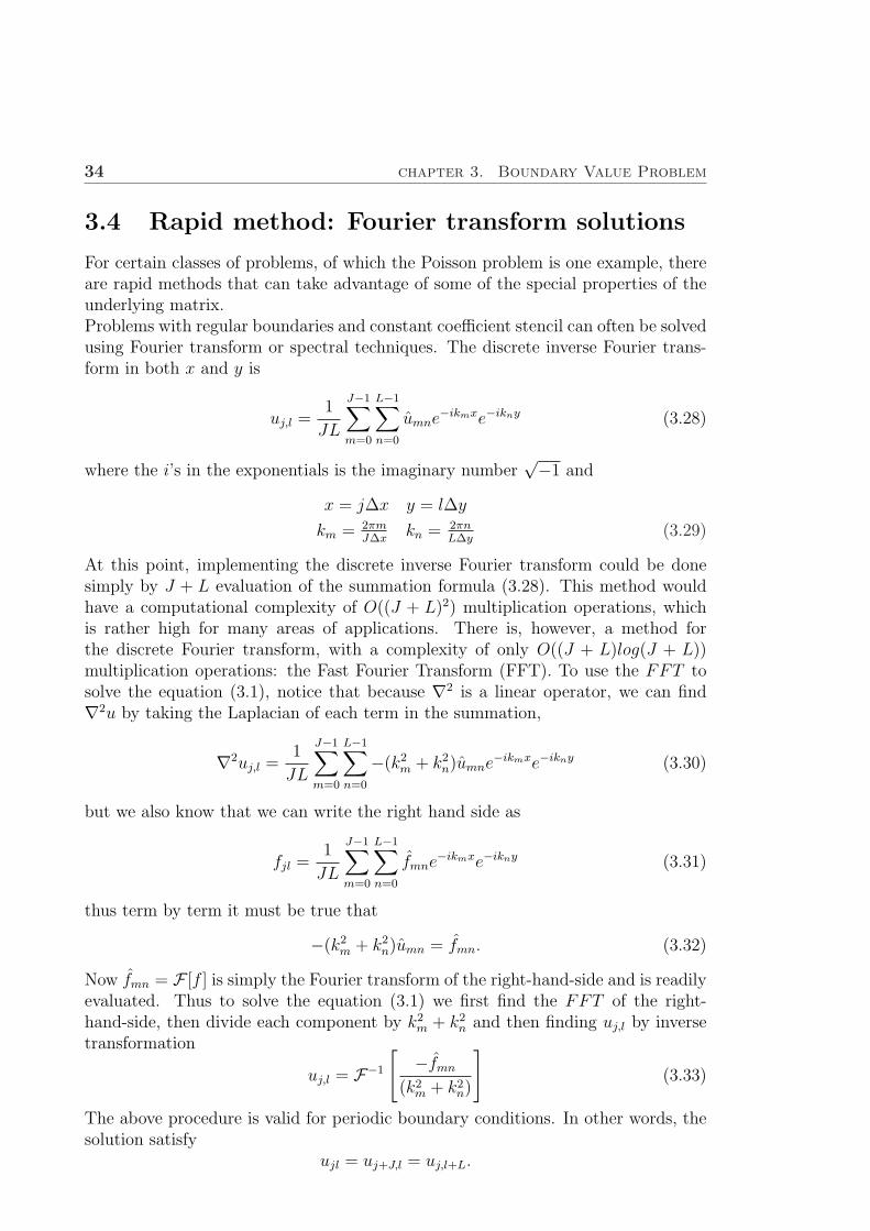
3.4 Rapid method: Fourier transform solutions

For certain classes of problems, of which the Poisson problem is one example, thereare rapid methods that can take advantage of some of the special properties of theunderlying matrix.Problems with regular boundaries and constant coefficient stencil can often be solvedusing Fourier transform or spectral techniques. The discrete inverse Fourier trans-form in both x and y is

uj,l =1

JL

J−1∑m=0

L−1∑n=0

umne−ikmxe−ikny (3.28)

where the i’s in the exponentials is the imaginary number√−1 and

x = j∆x y = l∆y

km = 2πmJ∆x

kn = 2πnL∆y

(3.29)

At this point, implementing the discrete inverse Fourier transform could be donesimply by J + L evaluation of the summation formula (3.28). This method wouldhave a computational complexity of O((J + L)2) multiplication operations, whichis rather high for many areas of applications. There is, however, a method forthe discrete Fourier transform, with a complexity of only O((J + L)log(J + L))multiplication operations: the Fast Fourier Transform (FFT). To use the FFT tosolve the equation (3.1), notice that because ∇2 is a linear operator, we can find∇2u by taking the Laplacian of each term in the summation,

∇2uj,l =1

JL

J−1∑m=0

L−1∑n=0

−(k2m + k2

n)umne−ikmxe−ikny (3.30)

but we also know that we can write the right hand side as

fjl =1

JL

J−1∑m=0

L−1∑n=0

fmne−ikmxe−ikny (3.31)

thus term by term it must be true that

−(k2m + k2

n)umn = fmn. (3.32)

Now fmn = F [f ] is simply the Fourier transform of the right-hand-side and is readilyevaluated. Thus to solve the equation (3.1) we first find the FFT of the right-hand-side, then divide each component by k2

m + k2n and then finding uj,l by inverse

transformation

uj,l = F−1

[−fmn

(k2m + k2

n)

](3.33)

The above procedure is valid for periodic boundary conditions. In other words, thesolution satisfy

ujl = uj+J,l = uj,l+L.

Section 3.5. The fast Fourier transform (FFT) 35

For Dirichlet boundaries where u = 0 we need expand the function in terms ofdiscrete sin series:

ujl =2

J

2

L

J−1∑m=1

L−1∑n=1

umnsin

(πjm

J

)sin

(πln

L

)(3.35)

this satisfy the boundary condition that u = 0 at j = 0, J and at l = 0, L. If wesubstitute this expansion and the analogous one for fjl into equation (3.1), we findthat the solution procedure is the same that for periodic boundary conditions.These and more general boundary conditions are discussed in some detail in [41].

3.5 The fast Fourier transform (FFT)

In 1965 J.W. Cooley and J. W. Tukey published a paper [59] about a special discreteFourier transform algorithm which they called fast Fourier transform. It was thispaper which caused the widespread dissemination of the FFT [60; 61] algorithm andnowadays it is one of the truly great computational developments of this century.The description of the FFT algorithm given in this section is based on the followingproof of the Daniel-Lanczos lemma, which makes it possible to write a discreteFourier transform length N (N even) as a sum of two discrete Fourier transforms oflength N/2:

Fk =N−1∑j=0

e2πijk/Nfj

=

N/2−1∑j=0

e2πi(2j)k/Nf2j +

N/2−1∑j=0

e2πi(2j+1)k/Nf2j+1

=

N/2−1∑j=0

e2πijk/(N/2)f2j + W k

N/2−1∑j=0

e2πijk/(N/2)f2j+1 (3.36)

= F ek + W kF o

k .

F ek (F o

k ) denotes the kth component of the Fourier transform of length N/2 formedfrom the even (odd) components of the original fj’s. The transforms F e

k and F ok

are periodic in k with period N/2, again, the required N components for Fk areobtained.If N/2 is even, (3.36) can be used again on F e

k and F ok . In the next step the F e

k

becomes the two Fourier transforms F eek and F eo

k of length N/4. For N = 2r (withr ∈ N) this can be carried out recursively r times, until identities of the formF eooe···oee

k = fn for any n are achieved. At this point the patterns of the e and oare changed to e = 0 end o = 1. From this point on, this operation is called abit reversal permutation. If the resulting sequence of bits is interpreted as a binarynumber, then it is exactly n. It is because of the successive subdivisions of the datainto even and odd values that is equivalent to the testing of the least significant bit

36 chapter 3. Boundary Value Problem

of the binary representation of n.Therefore, the first part of the FFT algorithm is to interchange fn using a bit reversalpermutation. The second part has an outer loop which is executed log2N times andcalculates, in turn, transform of length 2, 4, 8, · · · , N . At each stage of this process,two nested inner loops range over the sub-transforms already computed and theelements of each transform implementing the Daniel-Lanczos lemma (3.36). Duringeach stage O(N) arithmetic operations are carried out. Since there are log2N stages,the complexity of the whole FFT algorithm is of the order O(NlogN).

3.6 Cyclic reduction solvers

Evidently the FFT method works only when the original PDE has constant co-efficients and regular boundaries. A more general set of rapid methods, howeverexists for problems that are separable, in the sense of separation of variables. Thesemethods include cyclic reduction. Numerical Recipes [41] gives a brief explanationof how these methods work which we do not repeat here. We will tell about a col-lection of codes called FISHPAK packages [62]. These are a collection of generalizedcyclic reduction Fortran routines for solving more general Helmholtz problems, 3-DCartesian coordinates and general 2-D separable elliptic problem, for any combi-nation of periodic or mixed boundary conditions. These codes are extremely fastwith solution time scaling like N2logN , but they were written back in the eightiesand the Fortran is inscrutable and therefore hard to modify for different boundaryconditions. In addition they still only work for separable problems and could not,for example solve the more general problem ∇ · k∇T = ρ for a space varying con-ductivity. However, the only solvers that can compete in time with these routinesand handle spatially varying coefficients are the iterative multi-grid solvers.

3.7 Explicit time-stepping procedure

In previous sections we have seen how we can solve a non-linear diffusion equationas well as the Poisson equation, so we have all the elements in order to study ourspecific problem. The latter we remember to be:

∂T

∂t= ∇2T +

∂ψ

∂y

∂T

∂x− ∂ψ

∂x

∂T

∂y(3.37)

∇2ψ = −Ra∂T

∂x, (3.38)

T (x, 0) = 1; T (x, 1) = 0, (3.39)

∂T

∂x(0, y) =

∂T

∂x(1, y) = 0. (3.40)

We first discretize equations (3.38)-(3.40) in space by using second-order centereddifferences at the grid point (i, j) for i = 1, ..., N − 1 and j = 1, ..., M − 1 (i = 0 orN or j = 0 or M represent the points on the boundary. In particular the advection

Section 3.7. Explicit time-stepping procedure 37

term is discretized using Arakawa scheme. The resulting equations are

∂tTij = G1(Tij, ψij) (3.41)

∇2ψij = −RaG2(Tij) (3.42)

where G1 and G2 represent finite difference approximation for all the terms exceptthe one with time derivative in (3.42) We use second-order forward and backwarddifferences for the boundary condition of T .We use a second-order predictor-corrector scheme to iterate in time

T n+1ij = T n

ij +∆t

2∇2T n

ij +∆t

2(3J(T n

ij, ψnij)− J(T n−1

ij , ψn−1ij )). (3.43)

More precisely, the scheme is implemented in the following way:I. Initialization of the temperature and stream function at the time step n and alsoat n − 1. We suppose that the temperature has a linear vertical distribution. Thestream function is identically zero.II. Evaluate the intermediate temperature T n+ 1

2 by solving the implicit diffusionequation in the horizontal direction for the first half time step

Tn+1/2ij = T n

ij +∆t

2∇2T n

ij +∆t

4(3J(T n

ij, ψnij)− J(T n−1

ij , ψn−1ij )) (3.44)

for i = 1, ..., N − 1 and j = 1, ..., M − 1.III. Implement lateral boundary conditions on T

n+1/2ij .

IV . Evaluate the temperature T n+1 solving the implicit diffusion equation alongthe vertical direction for the second half time step

T n+1ij = T

n+1/2ij +

∆t

2∇2T

n+1/2ij +

∆t

4(3J(T n

ij, ψnij)− J(T n−1

ij , ψn−1ij )) (3.45)

for i = 1, ..., N − 1 and j = 1, ..., M − 1.V . Implement top and bottom boundary conditions on T n+1

ij .V I. Solve

∇2ψn+1ij = −RaG2(T

n+1ij ). (3.46)

by the generalized cyclic reduction routine from the FISHPACK package.V II. Implement boundary conditions on ψn+1

ij .V III. Go to the next time step.

Chapter 4

From Stationary Convection toChaos

In this Chapter, we investigate the different behaviors of the flow patterns and heattransport in a square porous media uniformly heated from below. We start from theonset of convection to high Rayleigh number limit where the flow is chaotic. TheRayleigh number determines the nature of the flow and it characterizes the evolutionof the system, from conduction at Ra < 4π2, to vigorous convection, at higher val-ues. Using the numerical methods described in Chapter 3 we determine the Rayleighnumbers at several transitions, which modify significantly the characteristic of theflow and the heat transport. These transitions can be of two types. The first type isa decrease in the horizontal aspect ratio of the cells. The second type is from steadyto unsteady pattern. The present investigation considers value of Rayleigh numberstarting from 44 until 1200. It will be seen later that it is within this range thatthe transitions from steady to oscillatory convection and from oscillatory to chaoticconvection occur.

4.1 Results of numerical simulations

The onset of convection is defined when the parallel fringe pattern of the state ofpure heat conduction is slightly deformed to a wavy shape, indicating the appear-ance of a vertical flow component rising upward along one of the two vertical walls.At low Rayleigh number, Ra = 44, the convective flow begins in the most favorablemode for that value, that consists of a roll with its axis parallel to the shorter side ofthe box, namely the uni-cellular mode. The flow is steady. The single roll can turnclockwise or counterclockwise depending on the initial condition (we have addedsome noise to the initial linear temperature profile). In a single cell, the fluid isswept horizontally toward the lateral boundary. Due to buoyancy it rises and even-tually impacts the upper boundary layer in the corner where the side wall meets theupper surface of the cell. In this way the fluid carries heat flux away from the hotboundary layer. In that corner the fluid is redirected horizontally, subsequently itbecomes a dominant part of the fluctuation which sweeps along the upper boundary

39

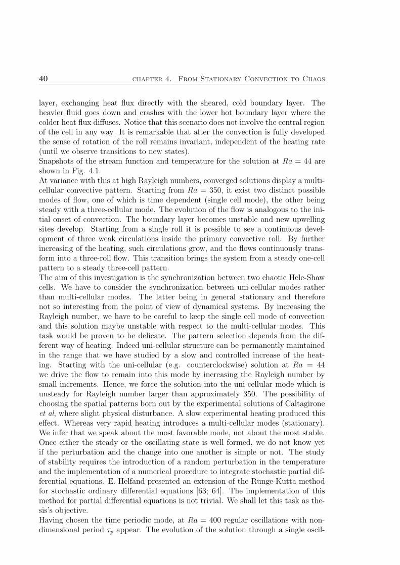
40 chapter 4. From Stationary Convection to Chaos

layer, exchanging heat flux directly with the sheared, cold boundary layer. Theheavier fluid goes down and crashes with the lower hot boundary layer where thecolder heat flux diffuses. Notice that this scenario does not involve the central regionof the cell in any way. It is remarkable that after the convection is fully developedthe sense of rotation of the roll remains invariant, independent of the heating rate(until we observe transitions to new states).Snapshots of the stream function and temperature for the solution at Ra = 44 areshown in Fig. 4.1.At variance with this at high Rayleigh numbers, converged solutions display a multi-cellular convective pattern. Starting from Ra = 350, it exist two distinct possiblemodes of flow, one of which is time dependent (single cell mode), the other beingsteady with a three-cellular mode. The evolution of the flow is analogous to the ini-tial onset of convection. The boundary layer becomes unstable and new upwellingsites develop. Starting from a single roll it is possible to see a continuous devel-opment of three weak circulations inside the primary convective roll. By furtherincreasing of the heating, such circulations grow, and the flows continuously trans-form into a three-roll flow. This transition brings the system from a steady one-cellpattern to a steady three-cell pattern.The aim of this investigation is the synchronization between two chaotic Hele-Shawcells. We have to consider the synchronization between uni-cellular modes ratherthan multi-cellular modes. The latter being in general stationary and thereforenot so interesting from the point of view of dynamical systems. By increasing theRayleigh number, we have to be careful to keep the single cell mode of convectionand this solution maybe unstable with respect to the multi-cellular modes. Thistask would be proven to be delicate. The pattern selection depends from the dif-ferent way of heating. Indeed uni-cellular structure can be permanently maintainedin the range that we have studied by a slow and controlled increase of the heat-ing. Starting with the uni-cellular (e.g. counterclockwise) solution at Ra = 44we drive the flow to remain into this mode by increasing the Rayleigh number bysmall increments. Hence, we force the solution into the uni-cellular mode which isunsteady for Rayleigh number larger than approximately 350. The possibility ofchoosing the spatial patterns born out by the experimental solutions of Caltagironeet al, where slight physical disturbance. A slow experimental heating produced thiseffect. Whereas very rapid heating introduces a multi-cellular modes (stationary).We infer that we speak about the most favorable mode, not about the most stable.Once either the steady or the oscillating state is well formed, we do not know yetif the perturbation and the change into one another is simple or not. The studyof stability requires the introduction of a random perturbation in the temperatureand the implementation of a numerical procedure to integrate stochastic partial dif-ferential equations. E. Helfand presented an extension of the Runge-Kutta methodfor stochastic ordinary differential equations [63; 64]. The implementation of thismethod for partial differential equations is not trivial. We shall let this task as the-sis’s objective.Having chosen the time periodic mode, at Ra = 400 regular oscillations with non-dimensional period τp appear. The evolution of the solution through a single oscil-

Section 4.1. Results of numerical simulations 41

a) b)

Figure 4.1: Stationary convection at Ra=44. a) The spatial pattern preferred by the flow is auni-cellular mode (stream-function). b) The snapshots of the temperature field show clockwise andcounterclockwise rotation of the roll.

lation period is illustrated in Fig. 4.2. The sequence is of five isothermal and fivestreamline plots evenly spaced in time (τp/4). The numerical simulation is char-acterized by one prevailing frequency, ω1 = 527.55 = 2π/τp. The power spectrum(defined as the squared modulus of the Fourier transform of the temperature takenat point x = 10/128,y=10/128), is particularly useful for determining the frequencyof a system. The power spectrum of the Nusselt number, plotted on log linear scale,shows characteristics of single periodic regime. Figure 4.2 exhibits sharp spectrallines, standing for the the dominant frequency and its harmonics. The power spec-trum of temperature is also peaked at the same frequency.The convective system departs from this single periodic state at Ra = 500 when

a second fundamental frequency, uncommensurable with the first, appears in thepower spectrum. A close look at the Poincare section [65] suggests a quasi-periodicdynamics. The concept of the Poincare section follows from the observation of asystem in the phase space and the consideration that the direction tangential to theflow (here flow refers to its meaning in the dynamical system theory) does not carrymuch interesting information. By a suitable oriented surface in the phase space, wecan construct an invertible map on this surface following a trajectory of the flow.The iterates of the map are given by the points where the trajectory intersects thesurface in a specified direction. In this way we reduce the phase space dimension-ally by one, at the same time turning the continuous time flow in a discrete timemap. The discrete time n of this map is the intersection count and is usually notsimply proportional to the continuous time t of the flow. The advantage of thePoincare section is that it permits to figure out the organization of the trajectoryin the phase space. At Ra = 520, (Fig. 4.3), we deduce that the phase trajectory is

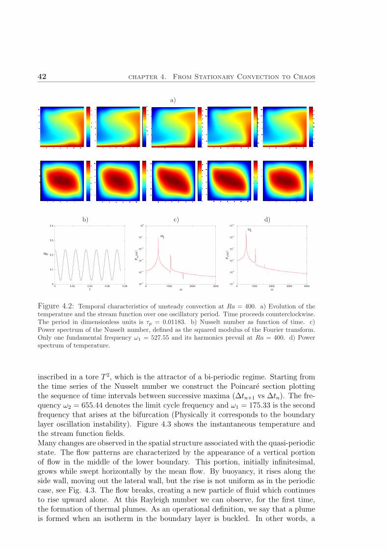
42 chapter 4. From Stationary Convection to Chaos

a)

b) c) d)

0 0.02 0.04 0.06 0.08

t

5

5.1

5.2

5.3

5.4

Nu

0 1000 2000 3000

ω

10−5

10−4

10−3

10−2

10−1

100

PN

u(ω

)

ω1

0 1000 2000 3000 4000

ω

10−7

10−6

10−5

10−4

10−3

10−2

PT(ω

)ω

1

Figure 4.2: Temporal characteristics of unsteady convection at Ra = 400. a) Evolution of thetemperature and the stream function over one oscillatory period. Time proceeds counterclockwise.The period in dimensionless units is τp = 0.01183. b) Nusselt number as function of time. c)Power spectrum of the Nusselt number, defined as the squared modulus of the Fourier transform.Only one fundamental frequency ω1 = 527.55 and its harmonics prevail at Ra = 400. d) Powerspectrum of temperature.

inscribed in a tore T 2, which is the attractor of a bi-periodic regime. Starting fromthe time series of the Nusselt number we construct the Poincare section plottingthe sequence of time intervals between successive maxima (∆tn+1 vs ∆tn). The fre-quency ω2 = 655.44 denotes the limit cycle frequency and ω1 = 175.33 is the secondfrequency that arises at the bifurcation (Physically it corresponds to the boundarylayer oscillation instability). Figure 4.3 shows the instantaneous temperature andthe stream function fields.Many changes are observed in the spatial structure associated with the quasi-periodicstate. The flow patterns are characterized by the appearance of a vertical portionof flow in the middle of the lower boundary. This portion, initially infinitesimal,grows while swept horizontally by the mean flow. By buoyancy, it rises along theside wall, moving out the lateral wall, but the rise is not uniform as in the periodiccase, see Fig. 4.3. The flow breaks, creating a new particle of fluid which continuesto rise upward alone. At this Rayleigh number we can observe, for the first time,the formation of thermal plumes. As an operational definition, we say that a plumeis formed when an isotherm in the boundary layer is buckled. In other words, a

Section 4.1. Results of numerical simulations 43

a)

b) c) d)

0 0.05 0.1 0.15 0.2

t

5.6

5.8

6

6.2

6.4

Nu

0 2000 4000 6000

ω

10−8

10−6

10−4

10−2

100

PN

u(ω

)

ω ω12

0.009 0.0093 0.0096 0.0099

∆tn

0.009

0.0093

0.0096

0.0099

∆tn+1

Figure 4.3: a) Snapshots of temperature and stream function for the solution at Ra = 520. Atthis value of the Rayleigh number, it appears for the first time thermal plumes. They are swepthorizontally in the lower boundary layer to rise along the right lateral wall by buoyancy. b) Nusseltnumber as function of time. c) The spectrum of Nu shows quasi-periodic behavior: ω2 = 655.44is the limit cycle frequency and ω1 = 175.33 is the second frequency that is born at the secondarybifurcation. d) Poincare section plots the typical ”eight” of a quasi-periodic state.

plume is formed when some portion of fluid becomes nearly vertical (away from thedownstream corner). In quasi-periodic cases, no plumes are identical. The hori-zontal position of each plume is shifted, so with each plume formation cycle differslightly in position relative to one another: each plume forms slightly upstream ordownstream of the main position of formation. This process occurs in the followingway: a fluctuation in the bottom boundary layer causes a plume to form just alittle bit earlier, causing a horizontal compression of the wave train (and verticalexpansion). This leads to two plumes being slightly closer to each other than theywould otherwise be. These two plumes together do a more efficient job of cleaningcold fluid of the boundary layer than usual. This leads to a little longer inductiontime for the next plume to form, a larger interval between plumes and a slightlyworse job of cleaning out the boundary layer. Thus the next plume forms a littleearlier and the flow develops a phase-modulated train of disturbance. We underlinethat the steady solution shows the same generation of two additional cells.Starting from Ra = 570 the solution returns back to a simply periodic regime. Thekey element is always the formation of thermal plumes, which change as Ra in-

44 chapter 4. From Stationary Convection to Chaos

a)

b) c) d)

0 0.01 0.02 0.03 0.04 0.05 0.06

t

10.3

10.4

10.5

10.6

10.7

Nu

0 10000 20000 30000

ω

10−8

10−6

10−4

10−2

100

PN

u(ω

)

ω1

0.002 0.003 0.004

∆tn

0.002

0.003

0.004∆t

n+

1

Figure 4.4: Same as figure 4.3 except that Ra = 900. a) Temporal evolution of the temper-ature and stream function over one oscillation period, τp = 0.00273. This time sequence of thetemperature shows the entire plume formation process. The overall circulation of the flow iscounterclockwise. b) Nusselt number as a function of time. c) At Ra = 900 a single frequency,ω1 = 2293.55, and its harmonic prevail. d) Poincare section.

creases. At Ra = 520 the plumes born around the middle of the bottom boundarylayer. They are small and grow, more in width than in height, as they are convectedacross the horizontal layer. At Ra = 900 the plumes start closer to the left lateralboundary with greater strength. They are narrow and expand vertically.Figure 4.4 shows, at Ra = 900, the evolution of the thermal plumes and stream

function over one oscillatory cycle. Every plume is identical, modulo a shift in time.The period, in dimensionless units, is equal to 0.00273. The power spectrum of theNusselt number has a single frequency, ω1 = 2293.55. The Poincare section is verysimple, it reduces to a point. The phase trajectory is a limit cycle.Starting from Ra = 1100, the scenario repeats. The numerical solution shows aquasi-periodic regime.At Ra = 1200 the amplitude of the variations in the heat transport reaches itsmaximum value and a strong broad band noise appears in the power spectrum,which is a characteristic of non-periodic motion. Exponential decay in the powerspectra at high frequency is expected for bounded smooth deterministic dynamics[66; 67]. The Poincare section shows a very large number of scattered points. The

Section 4.1. Results of numerical simulations 45

a)

b) c) d)

0 0.5 1 1.5 2

t

0.1

0.2

0.3

0.4

T

0 5000 10000 15000

ω

10−10

10−8

10−6

10−4

10−2

100

PT(ω)

0 0.002 0.004 0.006 0.008 0.01

∆tn

0

0.002

0.004

0.006

0.008

0.01

∆tn+1

Figure 4.5: Same as figure 4.3 except that Ra = 1200. No single frequency prevails in the powerspectrum anymore. b) Convection is in the chaotic regime. c) The power spectrum on a log linearscale illustrates the region of exponential decay. d) Poincare section showing the scattered points.

convective regime is now chaotic. Qualitatively, however, the flow patterns appearto follow a cycle, characterized also in this case by thermal plumes. The structureis similar to those at lower Rayleigh numbers, except that the plumes are very tightand stretched. This pattern repeats itself intermittently from the left of the lowerboundary without any specific regularity.In order to gain some knowledge about the time evolution of the system one can in-troduce some indicators as e. g. the autocorrelations of a signal [68; 69]. In general,the measurement sl of the state at time l is regarded from a probability distribution,p(s), for observing different values or sequences of value. The probability distribu-tion can be inferred from the time series. The mean of the probability distributioncan be estimated by the mean of the time series

< s >=1

N

L∑

l=1

sl (4.1)

where < · > denotes the average over time and L is the total number of mea-surements in the time series. The variance of the probability distribution will be

46 chapter 4. From Stationary Convection to Chaos

a) b)

0 50 100 150 200

τ

−1

−0.5

0

0.5

1

C(τ)

0 500 1000 1500 2000

τ

−1

−0.5

0

0.5

1

C(τ)

Figure 4.6: The autocorrelation function of the temperature signal at point x = 10/128; y =10/128. a) is close up of b), τ is the lag time (τ = ν∆t).

estimated by the variance of the time series

σ2 =1

N − 1

L∑

l=1

sl(sl− < s >)2. (4.2)

The autocorrelation at lag time ν is given by

cν =< (sl− < s >)(sl−ν− < s >) >

σ2. (4.3)

If we plot the values sl versus the corresponding values at fixed ν, the autocorrelationcν quantifies how these points are related. If they are not correlated then cν = 0.If the signal is observed over a continuous time, one can introduce autocorrelationfunction C(τ) and the correlation of equation (4.3) are estimates of C(τ = ν∆t).Obviously, C0 = 1.Autocorrelation of signals from chaotic systems decay exponentially with increasinglag time [65]. Our simulations indicate, indeed, that the correlation functions ofthe temperature, decay exponentially (at least for the envelope of the function).The spatial correlation function of the temperature has the same behavior. Figure4.7 shows the spatial correlation curves between points at three different heights(y = 1/4, y = 1/2 and y = 3/4).

0 0.2 0.4 0.6 0.8 1

ξ−0.5

0

0.5

1

C(ξ)

3/4

1/2

1/4

Figure 4.7: The spatial correlation function of the temperature for x ∈ [0, 1], at y = 1/4,y = 1/2 and y = 3/4.

Chapter 5

Synchronization

In the previous chapter we have shown that by heating uniformly from below anHele-Shaw cell a large number of different dynamical regimes may appear: station-ary convection, oscillatory convection, thermal plumes and turbulent flow. Thisrichness of different behaviors, in a rather simple geometry, seems a good candidatein order to study possible synchronization mechanisms between two identical cells.We give particular emphasis to the synchronization of chaotic dynamics. Indeed,this problem has attracted much attention during the last few years because of itsrole in the understanding of coupled nonlinear systems.In this context of different behaviors many different synchronization states havebeen identified: complete synchronization, phase synchronization, general synchro-nization, etc... [23].Here we have chosen to characterize the first discovered and certainly the simplestform of synchronization i.e. the complete synchronization.Different coupling schemes have been proposed in order to achieve synchronization.A widely used coupling, and controlling, technique is the so called “pinning” tech-nique [70; 71; 72; 73], which connects pair of points of the two systems.

5.1 Complete synchronization

For chaotic dynamics, synchronization influences not only the mean frequencies butalso the chaotic amplitudes. As a result, the signals coincide (or nearly coincide).Let us consider the temporal evolution of two identical chaotic systems:

x = f(x),

y = f(y), (5.1)

where x and y represent the N -dimensional state vectors of the systems, while fis a vector field f : Rn → Rn. As the dynamics of each variable is chaotic, inthe case of non interacting systems one sees two independent random-like processeswithout any mutual correlation. Now let us introduce an interaction between thetwo systems. Obviously, there is not a unique way to couple. However, we are

47

48 chapter 5. Synchronization

a) b) c)

−1

−0.5

0

0.5

1

ψ1

10.4

10.6

10.8

11

11.2

ψ1

10.4

10.6

10.8

11

11.2

ψ1

0 20 40t

0

0.3

0.6

ψ2

0 0.1t

10.4

10.6

10.8

11

11.2

ψ2

1.35 1.4 1.45 1.5t

10.4

10.6

10.8

11

11.2

ψ2

Figure 5.1: Time series of ψ1 and ψ2 at the point x = 1/3; y = 1/3. a) Complete synchronizationfor steady convection at Ra = 44. Complete synchronization for periodic convection at Ra = 400.b) At the beginning the time series are out of phase. c) Under the presence of the coupling theperiodic oscillations come in phase.

looking for a contractive coupling that tends to make the differences |x−y| smallerand does not affect the symmetric synchronous state x = y. Therefore, we demandthat the coupling force were proportional to the differences of the state of the twosystems and vanishes for coinciding state.A bidirectional coupling scheme is obtained by introducing the following additionaldissipation term:

x = f(x) + C · (y − x)

y = f(y) + C · (x− y) (5.2)

where C is a n× n matrix, whose coefficients rule the dissipative coupling. If thereis no coupling the two systems are completely independent and uncorrelated; withsmall coupling the trajectory of the signals will move closer due to the attractionbetween the two states. If the coupling is strong enough the attraction wins andeventually it can lead to a complete synchronized state.

5.1.1 All internal points are connectors

Starting from two identical Hele-Shaw cells, we introduce a thermal bidirectionalcoupling between all the internal points. Adding the dissipation term to the equa-tions (3.42) and (3.43), the systems are governed now by

I

∂T (1)

∂t= ∇2T (1) + J(T (1), ψ(1)) + ε(T (2) − T (1))

∇2ψ(1) = −RaG2(T(1))

Section 5.1. Complete synchronization 49

0 0.005 0.01 0.015 0.02

ε

0.85

0.9

0.95

1

1.05

γ

Figure 5.2: Pearson’s coefficient (see text for definition) vs the thermal coupling ε.

II

T (2)

∂t= ∇2T (2) + J(T (2), ψ(2)) + ε(T (1) − T (2))

∇2ψ(2) = −RaG2(T(2))

where the indexes 1 and 2 refer to the two systems, ε is the thermal coupling and isapplied in all the interior points (i, j = 1, ..., N − 1).Before presenting the results for the synchronization of chaotic systems, we want tobriefly discuss the cases of steady and periodic convection.At Ra = 44, two systems with a single convective cell, the first system with clockwiserotation, the second one with counterclockwise rotation are prepared. By setting thethermal coupling ε, which value lies in the interval [0.35, 1], synchronization betweenthe two cells is achieved. The cell of the first system begins to turn counterclockwise.The figure 5.1a shows complete coincidence of the two systems after some transient,for the coupling ε = 0.5.For the periodic case, Ra = 400, the two cells are prepared with counterclockwiserotation but they are initially out of phase, see Fig. 5.1b. This can be done bytaking as initial conditions for the second system the final state of the first aftera time of exactly half period. By applying a thermal coupling ε = 0.05 after 1000iterations, the two periodic states return in phase, see figure 5.1c. We underline thatthis is the simplest case. We pass through two different states of synchronization:from synchronization in anti-phase to synchronization in phase.Let us now come to discuss the case of chaotic dynamics at Ra = 1200. In this

case, the correlation function gains much interest because it is one central measurefor quantifying synchrony. Recent papers illustrate the power of the correlation inmeasuring the synchrony [74; 75; 76]. The most common way to quantify the degreeof synchronization between two variables is by monitoring the Pearson’s coefficientγ, or zero-lag cross-correlation

γ =< (T1− < T1 >)(T2− < T2 >) >

σ1σ2

(5.4)

where we recall that <> and σ2 denote a full space-time average and variance, re-spectively, and T1 and T2 are the temperature field of the two systems. Precisely,

50 chapter 5. Synchronization

a)

30 31 32 33 34 35

ψ1

28

30

32

34

36

ψ2

c)

28 30 32 34 36

ψ2

28

30

32

34

36

ψ1

b)

30

31

32

33

34

35

ψ1

0 0.02 0.04 0.06 0.08 0.1t

28

30

32

34

36

ψ2

d)

28

30

32

34

36

ψ1

0 0.02 0.04 0.06 0.08 0.1t

28

30

32

34

36

ψ2

Figure 5.3: a) Uncoupled Hele-Shaw cells, ψ1 vs ψ2 (ε = 0, x = 1/3; y = 1/3). b) Time series ofthe stream function below the synchronization threshold. c) and d) Complete synchronization incoupled Hele-Shaw cells (ε = 0.05). The states of the systems are identical.

when γ = 0 the two fields are linearly uncorrelated; γ = 1 marks complete corre-lation and γ = −1 indicates that the fields are negatively correlated. Figure 5.2reports the Pearson’s coefficient as function of the thermal coupling ε. The resultsindicate that for value of the coupling smaller than 0.02 the Pearson’s coefficient isalmost one. But, as we will see later, this not means the appearance of a completesynchronization state for these low values of the coupling.The cells have been prepared both with counterclockwise rotation but different ini-tial conditions. The proper way to do this is analog to what we did for the periodiccase. In order to see the differences between the systems we plot the variables ofsystem I vs the variables of system II, (a Lissajous-type plot) as in Fig. 5.3a. Ofcourse, the time series give us the same information as in Fig. 5.3b.We connect the two systems with couplings ε = 0.5, 0.05, 0.02, 0.01 at the dimen-

sionless time t = 0.01. Once we get synchronization, the states of the systems areidentical, as it can be easy seen on the plot ψ1 vs. ψ2, Fig. 5.3c. The trajectory lieson the diagonal ψ1 = ψ2. However, it is important to note that the coupling doesnot destroy the chaotic dynamics, but the oscillations are nearly identical, as shownin figure 5.3d.In order to verify the complete synchronization we have defined the synchronization

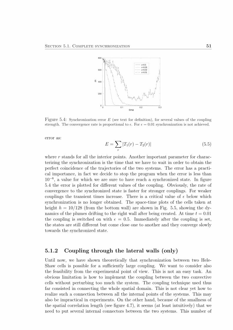
Section 5.1. Complete synchronization 51

0 0.1 0.2 0.3

time

0

200

400

600

800

E

ε=0.5ε=0.05ε=0.02ε=0.01

Figure 5.4: Synchronization error E (see text for definition), for several values of the couplingstrength. The convergence rate is proportional to ε. For ε = 0.01 synchronization is not achieved.

error as:

E =∑

r

|T1(r)− T2(r)| (5.5)

where r stands for all the interior points. Another important parameter for charac-terizing the synchronization is the time that we have to wait in order to obtain theperfect coincidence of the trajectories of the two systems. The error has a practi-cal importance, in fact we decide to stop the program when the error is less than10−6, a value for which we are sure to have reach a synchronized state. In figure5.4 the error is plotted for different values of the coupling. Obviously, the rate ofconvergence to the synchronized state is faster for stronger couplings. For weakercouplings the transient times increase. There is a critical value of ε below whichsynchronization is no longer obtained. The space-time plots of the cells taken atheight h = 10/128 (from the bottom wall) are shown in Fig. 5.5, showing the dy-namics of the plumes drifting to the right wall after being created. At time t = 0.01the coupling is switched on with ε = 0.5. Immediately after the coupling is set,the states are still different but come close one to another and they converge slowlytowards the synchronized state.

5.1.2 Coupling through the lateral walls (only)

Until now, we have shown theoretically that synchronization between two Hele-Shaw cells is possible for a sufficiently large coupling. We want to consider alsothe feasibility from the experimental point of view. This is not an easy task. Anobvious limitation is how to implement the coupling between the two convectivecells without perturbing too much the system. The coupling technique used thusfar consisted in connecting the whole spatial domain. This is not clear yet how torealize such a connection between all the internal points of the systems. This mayalso be impractical in experiments. On the other hand, because of the smallness ofthe spatial correlation length (see figure 4.7), it seems (at least intuitively) that weneed to put several internal connectors between the two systems. This number of

52 chapter 5. Synchronization

Figure 5.5: Space-time plots of the two convective cells at h = 10/128. At time t = 0.01 thecoupling (ε = 0.5) is switched on.

connectors must be finite and as small as possible. The reason for which we do notcouple in the whole spatial domain is that the uncoupled areas receive correlationwith the coupled areas that are in their neighborhood. They receive the informationabout the dynamics through the internal spatial diffusion inside the system. Inaddition we should mention also that the experimental measuring devices have afinite time resolution and measure local spatial information of some observable.Let us now give a brief account of the experiment. It has been thought to work byusing the Peltier effect in order to put or extract heat from the system. In 1934J. Peltier discovered that the passage of an electric current through the junctionof two dissimilar conductors can either cool or heat this junction, depending onthe direction of the current. Heat generation or absorption rates are proportionalto the magnitude of the current and also the temperature of the junction. Let usnow return to our numerical simulation, the cells are prepared with different initialconditions. Both cells have Peltier devices on each lateral boundary. The position ofthem is the same for the two cells. The temperature of the fluid around each Peltierdevice is constantly measured. A same fluid’s parcel has a different temperaturein the two cells. The Peltier device in contact with warmer fluid will extract heatand locally cools the surrounding fluid, the corresponding device in the other cellwill inject heat. This will last until the temperature measured in both systems areequilibrated.In order to test the feasibility of this experimental setup, we are using controllers

Section 5.1. Complete synchronization 53

0 0.1 0.2 0.3 0.4

time

0

1000

2000

3000

E

ε=0.3ε=3

Figure 5.6: Synchronization error using a weak and a very strong coupling connecting only thepoints located at the lateral boundaries. Synchronization is not achieved in these cases.

only belonging to the lateral walls i.e. 256 mesh points. With this particular choicethe systems are governed always by the same equations (5.3), where the term ε(T 2,1

i,j −T 1,2

i,j ) appears when i = 1, ..., N − 1, but only j = 1 and j = N − 1. An inspection ofthe synchronization errors suggest that this type of connection is not strong enoughto achieve synchronization. From Fig. 5.6, we observe that the synchronizationerror increases in time by using a very strong coupling, ε = 3.

5.1.3 Finite number of internal points are used as connec-tors

The failed attemp of synchronization through the lateral walls brings us to investi-gate the minimal number of “internal” points necessary in order to obtain synchro-nization. In experiment one will try to use as few controllers as possible.The simplest way to start investigating the minimal number of controllers is to put

the connectors every two grid points and, in case of success, following the reductionof connectors in this way. This strategy permits to get synchronization, but weobserve a change in the organization of the pattern structure, see figure 5.7. For aconnector every two grid points, the flow passes from a single roll cell (chaotic) to athree-cellular convection mode (stationary). The convergence to the synchronizationstate is not fast. Here the synchronization drastically affect the final dynamical stateof the system i.e. we have chaos suppression. Presumably, the basin of attraction ofthe single chaotic cell is quite narrow and a sparse and strong coupling will lead tofall in the three-cellular steady solution. The reason is that this solution is selectedwhen strong perturbations are applied to the single chaotic cell. In order to avoidto destroy the single cell solution, we have to increase very slowly the coupling fromzero to its nominal value. Unfortunately, all attempts to keep the single mode withless connectors have failed so far. Even worse, is the case of a connector every fourgrid points, in that case the synchronization is no longer achieved and the solutionsingle mode is destroyed into a two-cellular solution that is still chaotic.

54 chapter 5. Synchronization

Figure 5.7: The synchronization error obtained by connecting all the points, every two pointsand every four points. The coupling parameter, ε = 0.5, is set at t = 0.01. For a loose connection(every two points) a new three-cellular stationary structure appears. For a connector every fourpoints, synchronization is not achieved.

Conclusions, discussions andfurther works

In this work we have studied possible ways to synchronize two Hele-Shaw cells. Thisobjective has required first to study the dynamics of a single Hele-Shaw cell. TheHele-Shaw cell has been defined in the first chapter and it is interesting for us as asimple system possessing a boundary layer instability at reasonably large Rayleighnumber. There is no analytical tools available for solving nonlinear complicatedPDE. Therefore, in chapter 2 and 3, we have recalled the numerical techniquesthat permit to calculate the time evolution of the flow inside the convective cell.In Chapter 4, we have displayed the results of the integration of a Hele-Shaw cellfor different values of the Rayleigh number. By increasing this parameter, we passfrom stationary to oscillatory and chaotic convection with also formation of thermalplumes. Thermal plumes are generated in the lower unstable boundary layer.

One thing that comes clear from reading Chapter 4, is the dynamical richness ofthe Hele-Shaw cell. For a fixed value of the Rayleigh number, the system exhibitsmultistability. Several solutions are possible depending on the initial conditions.The question of stability of these multiple solutions has not been considered in thisthesis and is the first objective that we plan to pursue in the future. A “phase” dia-gram is the goal, i.e. for a fixed value of the Rayleigh number what are the solutionsstable and unstable and for each of the stable solution what is the basin of attractionof the solution. This study will certainly been time consuming but some tools canhelp in this task as e.g. Auto2000 [77] ( a bifurcation analysis package for ODE).In the same objective, we plan to perturb the solutions with different type of noise(starting from white Gaussian noise and then more complicated “colored” noise) inorder to study how robust the solutions are. In the process of drawing the “phase”diagram of the Hele-Shaw cell, it may be useful to reduce the PDE to a large set ofODE as it has been done by Dauby [78] in the case of Benard-Marangoni convectionin small containers.

We thought interesting to use the synchronization techniques in this realisticPDE system. In Chapter 5, we have presented some preliminary results on thesynchronization of two Hele-Shaw cells. Synchronization is possible if the cells arecoupled with all the internal points and a sufficient strong coupling. These require-ments are quite demanding and in view of future experimental realization not veryencouraging. Let us recall that synchronization through the lateral walls failed as

55

56 Conclusions, discussions and further works

well as for a loose coupling when only every 4 grid points were connected in space,as it is detailed in the end of Chapter 5. These first numerical results are not verypromising for experimental realization but we are planning to use a new techniquefor control based on the Floquet theory [79] that has permitted giant improvementin the control of spatial structures in semiconductor devices. Also in the connectionwith experiments, we want to use finite area of coupling rather than the less realistic“pinning” control used in Chapter 5, this will be based on some recent work of Jungeand Parlitz [72].

As it is often the case, this investigation has opened more doors than has givendefinitive answers.

Bibliography

[1] P. Berge and M. Dubois. Rayleigh-Benard Convection. Contemp. Phys., 25:535–582, 1984.

[2] H. Benard. Les tourbillons cellulaires dans une nappe liquide. Rev. Gen. Sci.Puers Appl., 11:1261–1271, 1900.

[3] Rayleigh, Lord. On convection currents in a horizontal layer of fluid when thehigher temperature is on the under side. Philos. Mag., 32:529–546, 1916.

[4] S.H. Davis. Convection in a box: linear theory. J. Fluid Mech., 30:465–478,1967.

[5] S.H. Davis. Convection in a box: on the dependence of preferred wave-numberupon the Rayleigh number at finite amplitude. J. Fluid Mech., 32:619–624,1968.

[6] E.L. Koschmieder. On convection on a uniformly heated plane. Beitr. Phys.Atmos., 39:1–11, 1966.

[7] E.L. Koschmieder. On convection on a non-uniformly heated plane. Phys. Rev.Lett., 39:208–216, 1966.

[8] J.N. Koster and U. Muller. Convection in boxes: an experimental investigationin vertical cylinder and annuli. J. Fluid Mech., 71:231–240, 1975.

[9] T. Ondarcuhu, J. Millan-Rodriguez, H. Mancini, A. Garciamartın and C. Perez-Garcia. Benard-Marangoni convective patterns in small cylindrical layers. Phys.Rev. E , 48:1051, 1993.

[10] M.L. Ramon, D. Maza and H. Mancini. Patterns in a small aspect ratio Benard-Marangoni convection. Phys. Rev. E , 60:4193–4198, 1999.

[11] J.N. Koster and U. Muller. Time-dependent free convection in vertical slots.Phys. Rev. Lett., 47:1599–1602, 1981.

[12] J. Bear. Dynamics of Fluid in Porous Media. New York, 1972.

[13] D.A. Nield and A. Bejan. Convection in Porous Media. New York, 1999.

[14] C.W. Horton and F.T. Rogers. . J. Appl. Phys., 16:367, 1945.

57

58 BIBLIOGRAPHY

[15] E.R. Lapwood. Convection of a fluid in a porous medium. Proc. Camb. PhilSoc., 44:508–521, 1948.

[16] J.P. Caltagirone, M. Cloupeau and M. Combarnous. Convection naturelle fluc-tuante dans une couche poreuse horizontale. Acad. Sci. Paris , 273:833–836,1971.

[17] R.N. Horne and M.J. O’Sullivan. Oscillatory convection in porous mediumheated from below. J. Fluid Mech., 66:339–352, 1974.

[18] A.S.M. Cherkaoui and W.S.D. Wilcock. Characteristics of high Rayleigh num-ber two-dimensional convection in an open-top porous layer heated from below. J. Fluid Mech., 394:241–260, 1999.

[19] M. P. Arroyo and J. M. Saviron. Rayleigh-Benard convection in a small box:spatial features and thermal dependence of the velocity field. J. Fluid Mech.,235:325–348, 1992.

[20] A. Pikovsky, M. Rosenblum and J. Kurths. Synchronization, A Universal Con-cept in Nonlinear Sciences . Cambridge University Press, UK, 2001.

[21] C. Huygens. Horologium Oscilatorium. Paris, France, 1673.

[22] L.M. Pecora and T.L. Carroll. Synchronization in chaotic systems. Phys. Rev.Lett., 64:821–824, 1990.

[23] S. Boccaletti, J. Kurts, G. Osipov, D.L. Valladares and C.S. Zhou. The syn-chronization of chaotic systems. Phys. Rep., 366:1–101, 2002.

[24] L. Kocarev and U. Parlitz. General approach for chaotic synchronization withapplications to communication. Phys. Rev. Lett., 74:5028–5031, 1995.

[25] U. Parlitz, L. Kocarev, T. Stojanovski and H. Preckel. Encoding messages usingchaotic synchronization. Phys. Rev. E , 53:4351–4361, 1996.

[26] S.H. Strogatz. Nonlinear Dynamics and Chaos . Addison–Wesley, USA, 1994.

[27] D. Pnueli and C. Gutfinger. Fluid Mechanics . Cambridge University Press,1992.

[28] R. Peyret. Spectral methods for incompressible viscous flow . Springer, NewYork, 2002.

[29] W.J. Minkowycz, E.M. Sparrow, G.E. Schneider and R.H. Pletcher. Handbookof numerical heat transfer . Wiley,New York, 1988.

[30] J.D. Lambert. Numerical methods for ordinary differential systems: the initialvalue problem. Wiley & Sons, London, 1991.

[31] R.D. Cook. Concept and applications of finite element analysis . Wiley & Sons,New York, 1981.

BIBLIOGRAPHY 59

[32] A.J. Davies. The finite element method: a first approach. Clarendon Press,Oxford, 1980.

[33] L.N. Trefthen. Spectral methods in MATLAB . PA: Society for Industial andApplied Mathematics, Philadelphia, 2000.

[34] B. Mercier. An introduction to numerical analysis of spectral methods . Springer,Berlin, 1989.

[35] D. Gottlieb and S.A. Orszag. Numerical analysis of spectral methods: theoryand application. Society for Industial and Applied Mathematics, Philadelphia,1993.

[36] C. Jordan. Calculus of finite differences . Chelsea publishing company, NewYork, 1965.

[37] L.M. Milne-Thomson. The calculus of finite differences . Macmillan and Co.,New York, 1965.

[38] G.D. Smith. Numerical solution of partial differential equations: finite differ-ence methods . Oxford University Press, New York, 1999.

[39] R. Courant. Differential and integral calculus . Interscience, 1970.

[40] E. Landau. Differential and integral calculus . Chelsea, New York, 1965.

[41] W.H. Press. Numerical recipes in FORTRAN: the art of scientific computing .Cambridge University Press, Cambridge, 1992.

[42] M. Spiegelman. Myths & Methods in Modeling . www.ldeo.columbia.edu/∼mspieg, 2000.

[43] W. E and J. Liu. Vorticity boundary condition and related isuue for finitedifference schemes . www.math.umd.edu/∼jliu/research, 2000.

[44] W. E and J. Liu. Essentially compact schemes for unsteady viscous incompress-ible flows . www.math.umd.edu/∼jliu/research, 2000.

[45] S. Weart. Arakawa’s Computation Trick . www.aip.org/history/climate, 2001.

[46] J.M. Beckers. Methodes numeriques appliquees a l’environnement .http://modb.oce.ulg.ac.be, 2002.

[47] J.M. Beckers. Mecanique des fluides non-homogenes .http://modb.oce.ulg.ac.be, 2000.

[48] G.H. Golub and C.G. Van Loan. Matrix Computations . Johns Hopkins Uni-versity Press, Baltimore, 1983.

[49] C.T. Kelley. Iterative Methods for Linear and Nonlinear equations . SIAM,Philadelphia, 1995.

60 BIBLIOGRAPHY

[50] C.W. Ueberhuber. Numerical Computation 2, Methods, Software and Analysis .Springer, Berlin, 1997.

[51] D.F. Elliot and K.R. Rao. Fast Transform: Algorithms, Analyses, Applications .Academic Press, New York, 1982.

[52] H.J. Nussbaumer. Fast Fourier Transform and Convolution Algorithms .Springer-Verlag, Berlin, 1981.

[53] C. Van Loan. Computational Framework for the Fast Fourier Transform. SIAMPress, Philadelphia, 1992.

[54] J.M. Lopez and J. Shen. An efficient spectral-projection method for the Navier-Stokes equations in cylindrical geometries. J. Comput. Phys., 139:308–326,1998.

[55] G.L. Brown and J.M. Lopez. Axisymmetric vortex breakdown, Part 2. Physicalmechanisms. J. Fluid Mech., 221:553–576, 1990.

[56] J.M. Lopez. Axisymmetric vortex breakdown, Part 1. Confined swirling flow.J. Fluid Mech., 221:533–552, 1990.

[57] J.M. Lopez and A.D. Perry. Axisymmetric vortex breakdown, Part 3. Onset ofperiodic flow and chaotic advection. J. Fluid Mech., 234:449–471, 1992.

[58] R.E. Lynch, J.R. Rice and D.H. Thomas. Direct solution of partial differentialequations by tensor product methods. Numer. Math., 6:185–199, 1964.

[59] J.W. Cooley and J.W. Tukey. An algorithm for the machine calculation ofcomplex Fourier series . Math. Comp., 19:297–301, 1965.

[60] E.O. Brigham. The fast Fourier transform. Englewood Cliffs: Prentice-Hall,1974.

[61] E.O. Brigham. The fast Fourier transform and its application. EnglewoodCliffs: Prentice-Hall, 1988.

[62] P.N. Swarztrauber and R.A. Sweet. Efficient FORTRAN subprograms for thesolution of elliptic partial differential equations. ACM Trans. Math. Soft., 5:352,1979.

[63] E. Helfand. Numerical integration of Stochastic Differential Equations . TheBell System Technical Journal , 58:2289–2299, 1979.

[64] E. Helfand. Numerical integration of Stochastic Differential Equations-II . TheBell System Technical Journal , 60:1927–1940, 1981.

[65] P. Berge, Y. Pomeau and C. Vidal. L’ordre dans le chaos. Vers une approchedeterministe de la turbulence. Hermann, Paris, 1984.

BIBLIOGRAPHY 61

[66] M.R. Paul, M.C. Cross, P.F. Fischer and H.S. Greenside. Power law behavior ofpower spectra in low Prandtl number Rayleigh Benard convection. Phys. Rev.Lett., 87:154501/1–4, 2001.

[67] U. Frisch and R. Morf. Intermittency in nonlinear dynamics and singularitiesat complex times. Phys. Rev. A, 23:2673–2705, 1981.

[68] H. Kantz and T. Schreiber. Nonlinear time series analysis . Cambridge Univer-sity Press, 1997.

[69] R. Hegger, H. Kantz and T. Schreiber. Practical implementation of nonlin-ear time series methods: The TISEAN package. www.mpipks-dresden.mpg.de,1998.

[70] G. Hu and Z. Qu. Controlling spatiotemporal chaos in coupled map latticesystems . Phys. Rev. Lett., 72:68–71, 1994.

[71] R.O. Grigoriev, M.C. Cross and H.G. Schuster. Pinning control of spatiotem-poral chaos . Phys. Rev. Lett., 79:2795–2798, 1997.

[72] L. Junge and U. Parlitz. Synchronization and control of coupled Ginzburg-Landau equations using local coupling. Phys. Rev. E , 61:3736–3742, 1999.

[73] S. Boccaletti, J. Bragard and F.T. Arecchi. Controlling and synchronizing spacetime chaos. Phys. Rev. E , 59:6574–6578, 1999.

[74] O.N. Bjornsatd, R.A. Ims and X. Lambin. Spatial population dynamics: ana-lyzing patterns and processes of population synchrony. Trends in ecology andevolution, 14:427–431, 2000.

[75] O.N. Bjornsatd and J. Bascompte. Synchrony and second-order spatial cor-relation in host-parasitoid systems . Journal of Animal Ecology , 70:924–933,2001.

[76] J. Bragard, S. Boccaletti and H. Mancini. Asymmetric coupling effects inthe synchronization of spatially extended chaotic systems . Phys. Rev. Lett.,91:064103, 2003.

[77] E. Doedel, R. Paffenroth, A. Champneys, T. Fairgrieve, Yu. Kuznetsov, B.Oldaman, S. Sonstade and X. Wong. Auto 2000: Continuation and bifurcationsoftware for ordinary differential equations (with Homcont). Technical Report,Concordia University, 2002.

[78] P.C. Dauby and L. Lebon. Benard-Marangoni instability in rigid rectangularcontainers. J. Fluid Mech., 329:25–64, 1996.

[79] N. Baba, A. Amann, E. Scoll and W. Just. Giant improvement of time-delayedfeedback control by spatio-temporal filtering. Phys. rev. Lett., 89:074101, 2002.