Angular momentum theory and applications

Gerrit C. GroenenboomTheoretical Chemistry, Institute for Molecules and Materials,

Radboud University Nijmegen, Heyendaalseweg 135,6525 ED Nijmegen, The Netherlands, e-mail: gerritg@theochem.ru.nl

(Dated: May 29, 2019)

Note: These lecture notes were used in a six hours course on angular momentum during the winter school onTheoretical Chemistry and Spectroscopy, Domaine des Masures, Han-sur-Lesse, Belgium, November 29 - December 3,1999. These notes are available from:http: // www. theochem. ru. nl/ cgi-bin/ dbase/ search. cgi? Groenenboom: 99

The lecture notes of another course on angular momentum, by Paul E. S. Wormer, are also on the web:http: // www. theochem. ru. nl/ ~ pwormer (Teaching material, Angular momentum theory). In those notes you canfind some recommendations for further reading.

Contents

I. Rotations 1A. Small rotations in SO(3) 2B. Computing eφN 4C. Adding the series expansion 4D. Basis transformations of vectors and operators 5E. Vector operators 6F. Euler parameters 8G. Rotating wave functions 8

II. Irreducible representations 9A. Rotation matrices 11

III. Vector coupling 14A. An irreducible basis for the tensor product space 14B. The rotation operator in the tensor product space 16C. Application to photo-absorption and photo-dissociation 18D. Density matrix formalism 18E. The space of linear operators 19

IV. Rotating in the dual space 20A. Tensor operators 21

Appendix A: exercises 22

I. ROTATIONS

Angular momentum theory is the theory of rotations. We discuss the rotation of vectors in R3, wave functions, andlinear operators. These objects are elements of linear spaces. In angular momentum theory it is sufficient to considerfinite dimensional spaces only.

• Rotations R are linear operators acting on an n−dimensional linear space V, i.e.,

R(~x+ ~y) = R~x+ R~y, Rλ~x = λR~x for all ~x, ~y ∈ V. (1)

2

We introduce an orthonormal basis {~e1, ~e2, . . . , ~en} so that we have

(~ei, ~ej) = δij , ~x =∑i

xi~ei, xi = (~ei, ~x). (2)

We define the column vector x = (x1, x2, . . . , xn)T , so that

~y = R~x, yi =∑j

Rijxj , Rij = (~ei, R~ej), y = Rx. (3)

Unless otherwise specified we will work in the standard basis {ei}. The multiplication of linear operators isassociative, thus for three rotations we have (R1R2)R3 = R1(R2R3).

• Rotations form a group:

– The product of two rotations is again a rotation, R1R2 = R3.

– There is one identity element R = I.

– For every rotation R there is an inverse R−1 such that RR−1 = R−1R = I.

• The rotation group is a three (real) parameter continuous group. This means that every element can be labeledby three parameters = (ω1, ω2, ω3). Furthermore, if

R(ω1) = R(ω2)R(ω3) (4)

we can express the parameters ω1 as analytic functions of ω2 and ω3. This means that we are allowed to takederivatives with respect to the parameters, which is the mathematical way of saying that there is such a thingas a “small rotation”. The choice of parameters is not unique for a given group.

• Rotations are unitary operators

(Rx, Ry) = (x,y), for all x and y. (5)

The adjoint or Hermitian conjugate A† of a linear operator A is defined by

(Ax,y) = (x, A†y), for all x and y. (6)

For the matrix elements of A† we have

(A†)ij = A∗ji. (7)

Hence, for a rotation matrix we have

(Rx, Ry) = (x, R†Ry) = (x,y), (8)

i.e., R†R = I, and R† = R−1. For the determinant we find

det(R†R) = det(R)∗ det(R) = det(I) = 1, |det(R)| = 1. (9)

By definition rotations have a determinant of +1.

• In R3 there is exactly one such group with the above properties and it is called SO(3), the special (determinantis +1) orthogonal group of R3. In C2 (two-dimensional complex space) there is also such a group called SU(2),the special (again since the determinant is +1) unitary group of C2. There is a 2:1 mapping between SU(2)and SO(3). The group SU(2) is required to treat half-integer spin.

A. Small rotations in SO(3)

By convention let the parameters of the identity element be zero. Consider changing one of the parameters (φ ∈ R).Since R(0) = I we can always write

R(ε) = I + εN. (10)

3

Since R†R = I we have

(I + εN)†(I + εN) = I + ε(N† +N) + ε2N†N = I, (11)

thus, for small ε

N† +N = 0, N† = −N. (12)

The matrix N is said to be antihermitian, N∗ij = −Nji. In R3 we may write

N =

0 −n3 n2

n3 0 −n1

−n2 n1 0

. (13)

The signs of the parameters are of course arbitrary, but with the above choice we have

Nx =

n2x3 − n3x2

n3x1 − n1x3

n1x2 − n2x1

= n× x. (14)

For small rotations we thus have

x′ = R(n, ε)x = x + εn× x. (15)

Clearly, the vector n is invariant under this rotation

R(n, ε)n = n + εn× n = n. (16)

For the product of two small rotations around the same vector n we have

R(n, ε1)R(n, ε2) = (I + ε1N)(I + ε2N) (17)

= I + (ε1 + ε2)N + ε1ε2N2 (18)

≈ R(n, ε1 + ε2). (19)

We now define non-infinitesimal rotations by requiring for arbitrary φ1 and φ2 that

R(n, φ1)R(n, φ2) = R(n, φ1 + φ2). (20)

We may now proceed in two ways to obtain an explicit formula for R(n, φ). First, we may observe that “many smallrotations give a big one”:

R(n, φ) = R(n, φ/k)k. (21)

By taking the limit for k →∞ and using the explicit expression for an infinitesimal rotation we get (see also AppendixA)

R(n, φ) = limk→∞

(I +φ

kN)k =

∞∑k=0

1

k!(φN)k = eφN . (22)

Note that a function of a matrix is defined by its series expansion.Alternatively we may start from eq. (20) and take the derivative with respect to φ1 at φ1 = 0 to obtain the

differential equation

d

dφ1R(n, φ1)|φ1=0R(n, φ2) =

d

dφ1R(n, φ1 + φ2)|φ1=0 =

d

dφ2R(n, φ2), (23)

with ddφ1

R(n, φ1) = N this gives

d

dφR(n, φ) = NR(n, φ). (24)

Solving this equation with the initial condition R(n, 0) = I again gives R(n, φ) = eφN .

4

B. Computing eφN

This problem is similar to solving the time-dependent Schrodinger equation, but it involves an antihermitian, ratherthan an Hermitian matrix. Therefore, we define the matrix Ln = iN , which is easily verified to be Hermitian

L† = (iN)† = −i(−N) = L. (25)

Thus, we have

R(n, φ) = e−iφL. (26)

The general procedure for computing functions of Hermitian matrices starts with computing the eigenvalues andeigenvectors

Lui = λiui. (27)

This may be written in matrix notation

LU = UΛ, U = [u1u2 . . .un], Λij = λiδij . (28)

For Hermitian matrices the eigenvalues are real and the eigenvectors may be orthonormalized so that U is unitaryand we have

L = UΛU†. (29)

If a function f is defined by its series expansion

f(x) =∑k

fkxk (30)

we have

f(L) =∑k

fkLk =

∑k

fk(UΛU†)k =∑k

fkUΛkU† = U(∑k

fkΛk)U† = Uf(Λ)U†. (31)

For the diagonal matrix Λ we simply have

[f(Λ)]ij =∑k

fk(λiδij)k =

∑k

fkλki δkij = f(λi)δij . (32)

Thus after computing the eigenvectors ui and eigenvalues λi of L we have

R(n, φ)x = e−iφLx = Ue−iφΛU†x =∑k

e−iφλkuk(uk,x). (33)

Note that the eigenvalues of R(n, φ) are e−iφλk . Since the λk’s are real, these (three) eigenvalues lie on the unit circlein the complex plane. Clearly, this must hold for any unitary matrix, since for any eigenvector u of some unitarymatrix U with eigenvalue λ we have

(Uu, Uu) = (λu, λu) = λ∗λ(u,u) = (u,u), i.e., |λ| = 1.. (34)

Note that R(n, φ)n = n. This does not yet prove that any R can be generated by an infinitesimal rotation. Since Ris real for every complex eigenvalue λ there must be an eigenvalue λ∗. The three eigenvalues lie on the unit circle inthe complex plane and their product is equal to the determinant (+1), therefore R must have at least one eigenvalueequal to 1. In this way, one can prove that any rotation is a rotation around some axis n.

C. Adding the series expansion

As an alternative approach we may start from

eφN =

∞∑k=0

1

k!(φN)k. (35)

5

From Eq. (27) it follows that

Nuk = −iλkuk ≡ αkuk. (36)

For the present discussion we will not actually need the eigenvectors and eigenvalues, we will only use the fact thatthey exist. We define the matrix A(N)

A(N) = (N − α1I)(N − α2I)(N − α3I). (37)

It is easily verified that for any eigenvector uk we have

A(N)uk = 0. (38)

Since any vector may be written as a linear combination of the eigenvectors uk we actually know that A(N) = 03×3,the zero matrix in R3. Thus, the polynomial A(N) is referred to as a annihilating polynomial. Expanding A(N) gives

A(N) = N3 + c2N2 + c1N + c0I = 0, (39)

where the coefficients ck can easily be expressed as functions of the eigenvalues αk. We now observe that N3 may beexpressed as a linear combination of lower powers of N :

N3 = −c2N2 − c1N − c0I (40)

From this equation we may directly compute the coefficients ck, without knowing the eigenvalues αk. By directmultiplication we construct the matrices Nk, k = 2, 3. By putting the matrix elements of these matrices in columnvectors of length 3× 3 = 9 we can turn the matrix equation into a set of 9 equations with 3 unknowns ck, k = 0, 1, 2.It may be of interest to know that this procedure is quite general: for a completely arbitrary n × n matrix A in Cn

there exist an annihilating polynomial of degree n. It can always be found be plugging the matrix A back into thecharacteristic polynomial P (λ) ≡ det(A− λI). In this case we have (see Appendix A)

N3 = −N. (41)

so that

N2k+1 = (−1)kN for k ≥ 0 (42)

N2k+2 = (−1)kN2 for k ≥ 1. (43)

As a consequence, the infinite sum simplifies to

eφN = I +

∞∑k=1

1

k!φkNk = I + sinφN + (1− cosφ)N2. (44)

D. Basis transformations of vectors and operators

We will refer to the basis {ek} used so far as the space fixed basis. We now introduce a new orthonormal basis{b} which we will refer to as the body fixed basis. These names are chosen with a typical application in a quantummechanical problem in mind. If the body fixed coordinates are indicated with a prime we have∑

k

ekxk =∑k

bkx′k, x = Bx′. (45)

Let a linear operator A be represented by the matrix A in the space fixed basis. We now define a transformed orrotated operator A′, which is represented by the matrix A′ in space fixed coordinates, by the requirement that it isrepresented by the matrix A when expressed in body fixed coordinates:

(bi, A′bj) = Aij , B†A′B = A. (46)

Using the unitarity of B we get

A′ = BAB†. (47)

6

Using this definition we may also transform any function of A defined by its series expansion

f(A)′ = Bf(A)B† = B(∑k

fkAk)B† =

∑k

fk(BAkB†) =∑k

fk(A′)k = f(A′). (48)

As an example we consider the transformation of a rotation operator

R′ = BR(n, φ)B† = BeφNB† = eφBNB†. (49)

We work out the exponent by considering

BNB†x = B(n×B†x) (50)

For an arbitrary unitary transformation of a cross product we have the rule (see Appendix A)

Ux× Uy = det(U)U(x× y) (51)

so that we have

B(n×B†x) = (Bn)× (BB†x) = (Bn)× x ≡ NBnx (52)

Thus, with the notation Nn = N ,

BNnB† = NBn (53)

and for the transformed rotation

BR(n, φ)B† = eφBNnB†

= R(Bn, φ). (54)

E. Vector operators

Define the three matrices Ni ≡ Nei. The matrix N can now be expressed as a linear combination of these matrices

N =

0 −n3 n2

n3 0 −n1

−n2 n1 0

= n1

0 0 00 0 −10 1 0

+ n2

0 0 10 0 0−1 0 0

+ n3

0 −1 01 0 00 0 0

(55)

= n1N1 + n2N2 + n3N3 = n ·N, (56)

where we introduced the vector operator N . The components of the vector operator transform as

BNjB† = BNejB

† = NBej = Nbj = bj ·N =∑i

NiBij . (57)

We also define the Hermitian vector operator L = iN for which we also have

BLjB† =

∑i

LiBij (58)

Since B is an arbitrary orthonormal matrix we may take B = R(n, φ) = e−iφn·L which gives

e−iφnLLjeiφnL =

∑i

LiRij(n, φ) (59)

For two operators A and B we have a relation which is sometimes referred to as the Baker-Campbell-Hausdorffform (appendix A)

eABe−A =

∞∑k=0

1

k![A,B]k, (60)

7

where the repeated commutator [A,B]k is defined by

[A,B]0 = B

[A,B]1 = [A,B] = AB −BA (61)

[A,B]k = [A, [A,B]k−1]. (62)

The importance of this relation is that the (repeated) commutation relations fully define the exponential form. Hence,from Eq. (59) we find for arbitrary angular momentum operators

R(n, φ)jR†(n, φ) = RT (n, φ)j. (63)

The commutation relations of two arbitrary antihermitian matrices Na and Nb follow from a property of the crossproduct (see appendix A)

x× (y × z) + y × (z× x) + z× (x× y) = 0. (64)

Using the property x× y = −y × x we find

a× (b× x)− b× (a× x)− (a× b)× x = 0. (65)

In matrix notation this gives

NaNbx−NbNax−Na×bx = 0. (66)

Since this holds for any x we obtain the commutation relation

[Na, Nb] = Na×b. (67)

The cross product of two basis vectors in an orthonormal basis may be written using the Levi-Civita tensor (e123 = 1,it changes sign when two indices are permuted),

ei × ej =∑k

eijkek, (68)

so that we can write the commutation relations for the components of the vector operator N as

[Ni, Nj ] =∑k

eijkNk. (69)

From this equation we immediately find the commutation relations for the Hermitian operators Li as

[Li, Lj ] =∑k

ieijkLk. (70)

These commutation relations, together with Eq. (60) allow us to write the left hand side of Eq. (59) as a linearcombination of the operators Li. The right hand side is also a linear combination of the operators Li. Thus, we canimmediately solve for the matrix elements Rij(n, φ), whenever the operators Li are linearly independent (i.e., when∑k akLk = 0⇒ ak = 0).One other example of Hermitian operators satisfying the commutation relations Eq. (70) are the generators of

SU(2),

σ1 =1

2

[0 11 0

], σ2 =

1

2

[0 −ii 0

], σ3 =

1

2

[1 00 −1

]. (71)

Note that e−i(φ+2π)σk = −e−iφσk . This is in agreement with the 2 : 1 mapping between SU(2) and SO(3) mentionedearlier.

8

F. Euler parameters

So far we have used the (n, φ) parameterization of SO(3). Since Euler parameters are used widely we describethem here. A linear operator in R3 is defined by its action on the three basis vectors. Let us assume that a rotationoperator R maps the basis vector e3 onto e′3. We can then write the matrix R as

R = R(e′3, γ)R1, (72)

where R1 may be any rotation for which e′3 = R1e3. If the polar angles of e′3 are (β, α) we can take

R1 = R(e3, α)R(e2, β). (73)

Thus, any rotation R can be written as

R(α, β, γ) = R(R1e3, γ)R1 = R1R(e3, γ)R†1R1, (74)

so that and

R(α, β, γ) = R(e3, α)R(e2, β)R(e3, γ) (75)

From this derivation we see that the ranges of the parameters required to span SO(3) are

0 ≤ α < 2π, 0 ≤ β < π, 0 ≤ γ < 2π. (76)

For the inverse we have

R(α, β, γ)−1 = R(e3,−γ)R(e2,−β)R(e3,−α). (77)

We may bring −β back into the range [0, π] by inserting R(e3, π)R(e3,−π) at both sides of R(e2,−β)twice and byusing the relation

R(e3,−π)R(e2,−β)R(e3, π) = R(−e2,−β) = R(e2, β), (78)

which gives

R(α, β, γ)−1 = R(e3,−γ + π)R(e2, β)R(e3,−α− π). (79)

We may also define a volume element for integration

dτ = dα sinβdβ dγ, (80)

which has the important property that for any function f(α, β, γ) the integral is invariant under rotation of thefunction f . The definition of a “rotated function” is given in the next section.

G. Rotating wave functions

We may extend the definition of rotations in R3 to the rotation of one particle wave functions (Ψ(x)) by Wigner’sconvention

(RΨ)(x) ≡ Ψ(R−1x). (81)

Usually, Ψ will be an element of some Hilbert space. For our purposes it is sufficient to think of Ψ as an element ofsome finite dimensional linear space V. Of course, we must assume that RΨ is also an element of V, whenever Ψ ∈ V.We use the hat ( ) to distinguish the operators on V from the corresponding operators in R3.

The inverse in the definition is important since it gives

R1(R2Ψ) = (R1R2)Ψ. (82)

This is readily verified:

[R1(R2Ψ)](x) = (R2Ψ)(R−11 x) = Ψ(R−1

2 R−11 x) = Ψ[(R1R2)−1x] = [(R1R2)Ψ](x). (83)

9

Note that Wigner’s convention is consistent with Dirac notation

Ψ(x) = 〈x|Ψ〉, 〈x|RΨ〉 = 〈R†x|Ψ〉 = 〈R−1x|Ψ〉. (84)

For small rotations we have

R(n, ε)Ψ(x) = Ψ(x− εn× x). (85)

To first order in ε we have in general

f(x + εy) = f(x) +∑k

εyk∂

∂xkf(x) ≡ f(x) + εy · ∇f(x), (86)

so that we may write

f(x− εn× x) = [1− ε(n× x) · ∇]f(x). (87)

Using n× x · ∇ = eijknixj∇k = n · x×∇ we find

R(n, ε) = 1− εn · x×∇ = 1− iεn · L, (88)

where we defined

p ≡ −i∇ (89)

L ≡ x× p. (90)

Using integration by parts, and assuming that the surface term vanishes, it is easy to show that the operators ∇k areantihermitian, i.e. (∇kf, g) = (f,−∇kg). The multiplicative operators xk are Hermitian and it is also straightforward

to evaluate the commutator [∇i, xj ] = δij . It is left as an exercise for the reader to verify that the operators Lk areHermitian and that they satisfy the commutation relations

[Li, Lj ] = i∑k

eijkLk. (91)

We may now follow the same procedure as before to find the expression for a non-infinitesimal rotation

R(n, φ) = e−iφn·L. (92)

If we choose a n dimensional (orthonormal) basis {|i〉, i = 1, . . . , n} in the space V we may represent the operators R

and Lk by n dimensional matrices. For rotations we will denote these matrices as D(R). By definition

Dij(R) = 〈i|R|j〉. (93)

We also use the notation D(n, φ) = D[R(n, φ)]. The unitary matrices D(R) are a representation of SO(3), since

R(n1, φ1)R(n2, φ2) = R(n3, φ3) (94)

implies

D(n1, φ1)D(n2, φ2) = D(n3, φ3). (95)

This representation may be reducible. That is, it may be possible to find a unitary transformation of the basis thatwill simultaneously block diagonalize the matrices D(R) for all R.

II. IRREDUCIBLE REPRESENTATIONS

Suppose we can divide the space V into a subspace S and its orthogonal complement T , i.e. S ⊕ T = V, such thatfor all Ψ ∈ S and for all R(n, φ) we have RΨ ∈ S. In this case S is called an invariant subspace. Since the operators

R are unitary T must also be an invariant subspace. If not, we could find some f ∈ T and g ∈ S such that for someR we would have (g, Rf) 6= 0. However, that would mean that (R−1g, f) 6= 0, which is in contradiction with S being

10

an invariant subspace. Thus, if we construct a basis {|i〉, i = 1, . . . , n} where the first m vectors {|i〉, i = 1, . . . ,m}span the space S and the vectors {|i〉, i = m+ 1, . . . , n} span the space T we find that all matrices D(R) have a blockstructure.

Suppose some Hermitian operator A commutes with all operators R(n, φ)

[A, R(n, φ)] = 0. (96)

Let Sλ be the space spanned by all eigenvectors fi with eigenvalue λ

Afi = λfi. (97)

For each each f ∈ Sλ we find that g = Rf also has eigenvalue λ

Ag = ARf = RAf = λg, (98)

i.e., g ∈ Sλ, which shows that Sλ is an invariant subspace. In order to find an operator A that commutes with eachR it is sufficient to find an operator that commutes with L1, L2, and L3.

From the commutation relations of Lk we can show that the Hermitian operator

L2 = L21 + L2

2 + L23 (99)

commutes with L1, L2, and L3. It turns out that the commutation relations also allow us to derive the possibleeigenvalues of L2 and the dimensions of the subspaces. Furthermore, within each eigenspace of L2 we can constructa basis of eigenfunctions of the L3 operator and we can even derive the matrix elements of all operators Lk in thisbasis. We summarize this general result:

A linear (or Hilbert) space V which is invariant under the Hermitian operators ji, i = 1, 2, 3 that satisfy thecommutation relations

[ji, jj ] = i∑k

εijk jk (100)

decomposes into invariant subspaces Vj of j2 = j21 + j2

2 + j23 . The spaces Vj are spanned by orthonormal kets

|j,m〉, m = −j, . . . , j, (101)

with

j2|j,m〉 = j(j + 1)|j,m〉, (102)

j3|j,m〉 = m|j,m〉, (103)

j±|j,m〉 = C±(j,m)|j,m± 1〉, (104)

with

j± = j1 ± ij2 (105)

C±(j,m) =√j(j + 1)−m(m± 1). (106)

The j± are the so called step up/down operators.The proof of the existence of basis (101) is well-known. Briefly, the main arguments are:

• As [j2, j3] = 0, we can find a common eigenvector |a, b〉 of j2 and j3 with j2|a, b〉 = a2|a, b〉 and j3|a, b〉 = b|a, b〉.Since it is easy to show that j2 has only non-negative real eigenvalues, we write its eigenvalue as a squarednumber.

• Considering the commutation relations [j3, j±] = ±j± and [j2, j±] = 0, we find, that j2j+|a, b〉 = a2j+|a, b〉 and

j3j+|a, b〉 = (b+ 1)j+|a, b〉. Hence j+|a, b〉 = |a, b+ 1〉

• If we apply j+ now k + 1 times we obtain, using j†+ = j−, the ket |a, b+ k + 1〉 with norm

〈a, b+ k|j−j+|a, b+ k〉 = [a2 − (b+ k)(b+ k + 1)]〈a, b+ k|a, b+ k〉. (107)

Thus, if we let k increase, there comes a point that the norm on the left hand side would have to be negative(or zero), while the norm on the right hand side would still be positive. A negative norm is in contradictionwith the fact that the ket belongs to a Hilbert space. Hence there must exist a value of the integer k, such thatthe ket |a, b+ k〉 6= 0, while |a, b+ k + 1〉 = 0. Also a2 = (b+ k)(b+ k + 1) for that value of k.

11

• Similarly l+ 1 times application of j− gives a zero ket |a, b− l− 1〉 with |a, b− l〉 6= 0 and a2 = (b− l)(b− l− 1).

• From the fact that a2 = (b+k)(b+k+1) = (b− l)(b− l−1) follows 2b = l−k, so that b is integer or half-integer.This quantum number is traditionally designated by m. The maximum value of m will be designated by j.Hence a2 = j(j + 1).

• Requiring that |j,m〉 and j±|j,m〉 are normalized and fixing phases, we obtain the well-known formula (105).

Summarizing, in V we have the basis {|j,m〉, j = 0, 12 , 1, . . . ;m = −j, . . . , j}. Not all values of j need to occur in a

given space V. The angular momentum operators are diagonal in j, and their matrix elements are

〈jm′|j2|jm〉 = j(j + 1)δm′m (108)

〈jm′|j1|jm〉 =1

2[C+(j,m)δm′,m+1 + C−(j,m)δm′,m−1] (109)

〈jm′|j2|jm〉 = −i12

[C+(j,m)δm′,m+1 − C−(j,m)δm′,m−1] (110)

〈jm′|j3|jm〉 = mδm′m. (111)

A. Rotation matrices

The rotation operators in V are, by definition

R(n, φ) = e−iφn·j . (112)

The matrix representation D(R) is block diagonal in j. The matrix elements of the diagonal blocks Dj are

Djk,m(n, φ) ≡ 〈jk|R(n, φ)|jm〉. (113)

Thus, for a rotated vector we have

R|jm〉 =∑k

|jk〉〈jk|R|jm〉 =∑k

|jk〉Djkm(R). (114)

The matrix elements of the rotation operator themselves can act as functions on which we may define the action of arotation operator according to Wigner’s convention:

R1Djmk(R2) = Dj

mk(R−11 R2) =

∑m′

Djmm′(R

−11 )Dj

m′k(R2). (115)

Here we used the general property of representations that D(R1R2) = D(R1)D(R2). When we compare this result

with Eq. (114) we find that the function Djm,k(R) almost behaves as a ket |jm〉, except that the inverse of R1 appears.

This can be remedied by starting with the complex conjugate of a D-matrix element:

R1Dj,∗mk(R2) =

∑m′

Dj,∗mm′(R

−11 )Dj,∗

m′k(R2) =∑m′

Dj,∗m′k(R2)Dj

m′m(R1). (116)

where we used another property of representations: D(R−1) = D(R)−1.Many properties of D-matrices are independent of the parameterization that we choose. However, if we do need a

parameterization, the Euler parameters are very useful, since they allow us to factorize any D-matrix in D-matricesdepending on a single parameter:

D[R(α, β, γ)] = D[R(e3, α)]D[R(e2, β)]D[R(e3, γ)] ≡ D(e3, α)D(e2, β)D(e3, γ). (117)

With the procedure for exponentiating an operator described in Section I B it is straightforward to derive

Djkm(e3, γ) = 〈jk|e−iγj3 |jm〉 = e−imγδkm. (118)

To find Dj(e2, β) we must exponentiate −iβj(j)2 , where j

(j)2 is the matrix representation of j2 in Vj . Note that this

matrix is real. Usually it is denoted by dj(β) ≡ Dj(e2, β) so that we have

Djmk(α, β, γ) = e−imαdjmk(β)e−ikγ . (119)

12

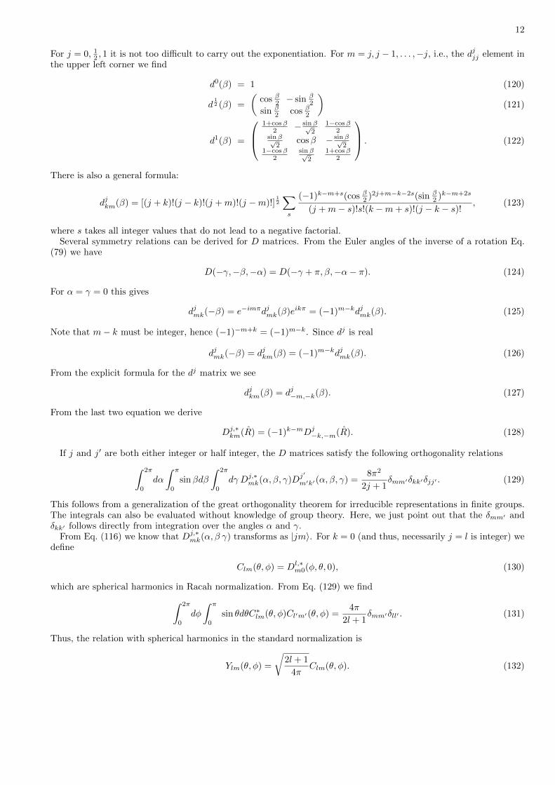
For j = 0, 12 , 1 it is not too difficult to carry out the exponentiation. For m = j, j − 1, . . . ,−j, i.e., the djjj element in

the upper left corner we find

d0(β) = 1 (120)

d12 (β) =

(cos β2 − sin β

2

sin β2 cos β2

)(121)

d1(β) =

1+cos β

2 − sin β√2

1−cos β2

sin β√2

cosβ − sin β√2

1−cos β2

sin β√2

1+cos β2

. (122)

There is also a general formula:

djkm(β) = [(j + k)!(j − k)!(j +m)!(j −m)!]12

∑s

(−1)k−m+s(cos β2 )2j+m−k−2s(sin β2 )k−m+2s

(j +m− s)!s!(k −m+ s)!(j − k − s)!, (123)

where s takes all integer values that do not lead to a negative factorial.Several symmetry relations can be derived for D matrices. From the Euler angles of the inverse of a rotation Eq.

(79) we have

D(−γ,−β,−α) = D(−γ + π, β,−α− π). (124)

For α = γ = 0 this gives

djmk(−β) = e−imπdjmk(β)eikπ = (−1)m−kdjmk(β). (125)

Note that m− k must be integer, hence (−1)−m+k = (−1)m−k. Since dj is real

djmk(−β) = djkm(β) = (−1)m−kdjmk(β). (126)

From the explicit formula for the dj matrix we see

djkm(β) = dj−m,−k(β). (127)

From the last two equation we derive

Dj,∗km(R) = (−1)k−mDj

−k,−m(R). (128)

If j and j′ are both either integer or half integer, the D matrices satisfy the following orthogonality relations∫ 2π

0

dα

∫ π

0

sinβdβ

∫ 2π

0

dγ Dj,∗mk(α, β, γ)Dj′

m′k′(α, β, γ) =8π2

2j + 1δmm′δkk′δjj′ . (129)

This follows from a generalization of the great orthogonality theorem for irreducible representations in finite groups.The integrals can also be evaluated without knowledge of group theory. Here, we just point out that the δmm′ andδkk′ follows directly from integration over the angles α and γ.

From Eq. (116) we know that Dj,∗mk(α, β γ) transforms as |jm〉. For k = 0 (and thus, necessarily j = l is integer) we

define

Clm(θ, φ) = Dl,∗m0(φ, θ, 0), (130)

which are spherical harmonics in Racah normalization. From Eq. (129) we find∫ 2π

0

dφ

∫ π

0

sin θdθC∗lm(θ, φ)Cl′m′(θ, φ) =4π

2l + 1δmm′δll′ . (131)

Thus, the relation with spherical harmonics in the standard normalization is

Ylm(θ, φ) =

√2l + 1

4πClm(θ, φ). (132)

13

Also setting m to zero gives us Legendre polynomials

Pl(cos θ) = dl00(θ) = Cl0(θ, φ). (133)

We also define the regular harmonics,

Rlm(r) = rlClm(r), (134)

where rT = (x, y, z) = r(cosφ sin θ, sinφ sin θ, cos θ), and r = (θ, φ). From the explicit formulas for D0 and D1 we find

R0,0(r) = 1 (135)

R1,1(r) = − 1√2

(x+ iy) ≡ r+1 (136)

R1,0(r) = z ≡ r0 (137)

R1,−1(r) =1√2

(x− iy) ≡ r−1. (138)

The r+1, r0, and r−1 are the so called spherical components of the vector r. They are related to the Cartesiancomponents via the unitary transformation

r ≡

r+

r0

r−

=

√1

2

−1 −i 0

0 0√

21 −i 0

xyz

≡ ST r. (139)

We put in the transpose so that for row vectors we get rT = rTS. We now compare the rotation of the Cartesian andthe spherical components of a vector. In Cartesian coordinates we define

r ≡ R(n, φ)r′, ⇒ r′T = rTR(n, φ) (140)

and for the spherical components we find

R(n, φ)Rlm(r) = Rlm[R(n, φ)−1r] = Rlm(r′) =∑k

Rlk(r)Dlkm(n, φ). (141)

For l = 1 this gives r′T = rTD1(n, φ), so that

r′T = r′TS = rTRS = rTSD1, (142)

which gives

R = SD1S†. (143)

We recall that the components of an angular momentum operator transform as the Cartesian components of a row

vector [see Eq. (59)]. Thus, if we define J(1)µ =

∑i JiSiµ, with µ = +1, 0,−1, i.e.,

J(1)+1 = −

√1

2(J1 + iJ2) (144)

J(1)0 = J3 (145)

J(1)−1 =

√1

2(J1 − iJ2) (146)

we obtain

R(n, φ)J (1)m R(n, φ)† =

∑k

J(1)k D1

km(n, φ). (147)

14

III. VECTOR COUPLING

In quantum chemistry one usually writes a two electron wave function as, e.g., ψa(r1)ψb(r2)−ψa(r2)ψb(r1). When-ever convenient, we will use tensor product notation where, by definition, we keep the order of the arguments fixed,so that we can drop them, and we write ψa ⊗ ψb − ψb ⊗ ψa. For two linear spaces V1 and V2 with dimensions n1, n2,the tensor product space V1⊗V2 is a n1×n2 dimensional linear space which contains the tensor products f ⊗ g, withf ∈ V1 and g ∈ V2. For a complete definition me must point out when two elements of V1 ⊗ V2 are the same:

(λf)⊗ g = f ⊗ (λg) = λ(f ⊗ g) (148)

(f + g)⊗ h = f ⊗ h+ g ⊗ h (149)

f ⊗ (g + h) = f ⊗ g + f ⊗ h. (150)

For linear operators A and B defined on V1 and V2, respectively, we define

(A⊗ B)(f ⊗ g) = (Af)⊗ (Bg). (151)

Thus, (∇x +∇y)f(x)g(y) written in tensor notation becomes (∇⊗ I + I ⊗∇)f ⊗ g.The scalar product in the tensor product space is defined in terms of the scalar products on V1 and V2 by

(f1 ⊗ g1, f2 ⊗ g2) = (f1, f2)(g1, g2). (152)

If we have an orthonormal basis {ei, i = 1, . . . , n1} on V1 and an orthonormal basis {fi, i = 1, . . . , n2} thenei ⊗ fj , i = 1, . . . , n1; j = 1, . . . , n2} forms an orthonormal basis for V1 ⊗ V2. Clearly, we have

(ei ⊗ fj , ei′ ⊗ fj′) = (ei, ei′)(fj , fj′) = δii′δjj′ . (153)

If the matrix elements Aij = (ei, Aej) and Bij = (fi, Bfj) are known, we can easily compute the matrix elements of

the tensor product A⊗ B in the tensor product basis

(ei ⊗ fj , [A⊗ B]ei′ ⊗ fj′) = (ei ⊗ fj , Aei′ ⊗ Bfj′) = (ei, Aei′)(fj , Bfj′) = Aii′Bjj′ . (154)

Let Afi = λifi and Bgj = µjgj , then

(A⊗ I + I ⊗ B)(fi ⊗ gj) = Afi ⊗ Igj + Ifi ⊗ Bgj = λifi ⊗ gj + µjfi ⊗ gj = (λi + µj)fi ⊗ gj , (155)

i.e., the functions fi ⊗ gj are eigenfunctions of the operator (A⊗ I + I ⊗ B) with eigenvalues (λi + µj).From the Taylor expansion of an exponential one can prove that, for scalars, ea+b = eaeb. Since functions of

operators are defined by the series expansion this relation also holds for operators that commute. It is readily verifiedthat the commutator

[A⊗ I , I ⊗ B] = 0 (156)

and so we have

eA⊗I+I⊗B = eA ⊗ eB . (157)

A. An irreducible basis for the tensor product space

Let us assume that Vj1 and Vj2 are spaces spanned by the bases {|j1,m1〉,m1 = −j1, . . . , j1} and {|j2,m2〉,m2 =−j2, . . . , j2}, respectively. All that we need to construct an irreducible basis for the tensor product space is a set ofthree Hermitian operators that satisfy the angular momentum commutation relations. It is not hard to verify thatthe operators

Ji ≡ ji ⊗ 1 + 1⊗ ji, i = 1, 2, 3 (158)

satisfy these conditions. Since we have explicit expressions for the matrix elements of ji in the bases of Vj1 and Vj2we can easily calculate the matrix elements of the operators Ji in the so called uncoupled basis

|j1m1j2m2〉 ≡ |j1m1〉 ⊗ |j2m2〉, m1 = −j1, . . . , j1; m2 = −j2, . . . , j2. (159)

15

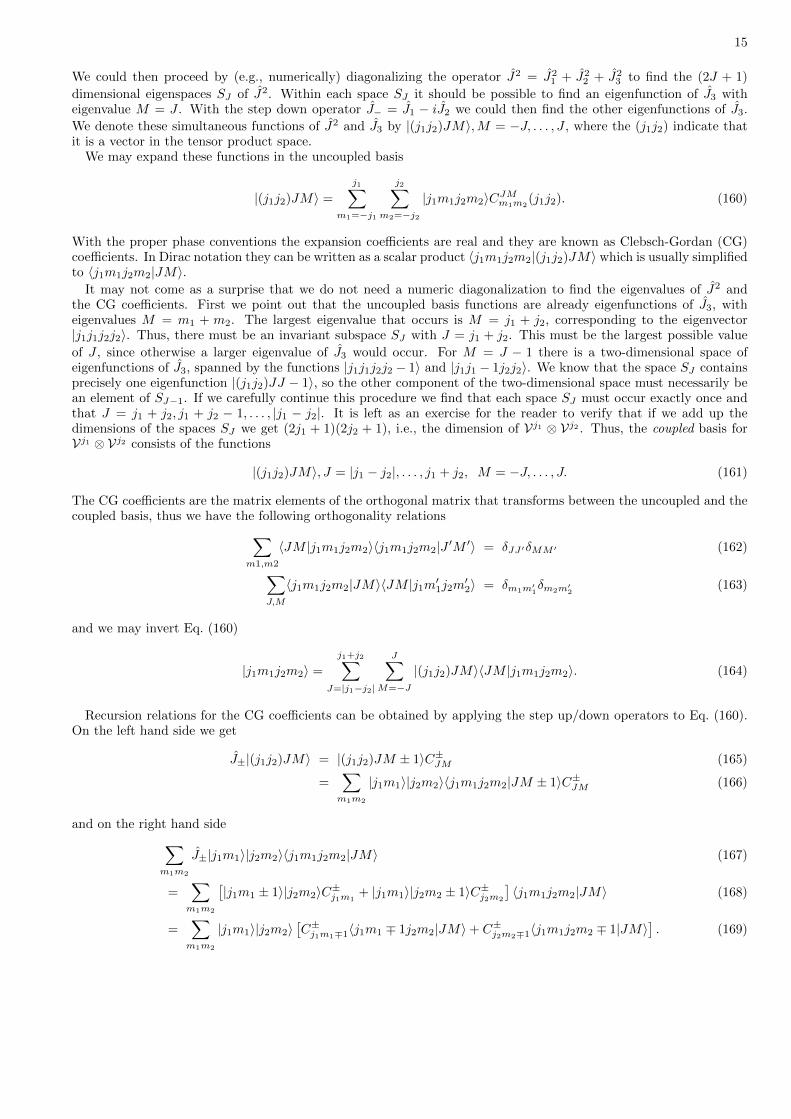
We could then proceed by (e.g., numerically) diagonalizing the operator J2 = J21 + J2

2 + J23 to find the (2J + 1)

dimensional eigenspaces SJ of J2. Within each space SJ it should be possible to find an eigenfunction of J3 witheigenvalue M = J . With the step down operator J− = J1 − iJ2 we could then find the other eigenfunctions of J3.

We denote these simultaneous functions of J2 and J3 by |(j1j2)JM〉,M = −J, . . . , J , where the (j1j2) indicate thatit is a vector in the tensor product space.

We may expand these functions in the uncoupled basis

|(j1j2)JM〉 =

j1∑m1=−j1

j2∑m2=−j2

|j1m1j2m2〉CJMm1m2(j1j2). (160)

With the proper phase conventions the expansion coefficients are real and they are known as Clebsch-Gordan (CG)coefficients. In Dirac notation they can be written as a scalar product 〈j1m1j2m2|(j1j2)JM〉 which is usually simplifiedto 〈j1m1j2m2|JM〉.

It may not come as a surprise that we do not need a numeric diagonalization to find the eigenvalues of J2 andthe CG coefficients. First we point out that the uncoupled basis functions are already eigenfunctions of J3, witheigenvalues M = m1 + m2. The largest eigenvalue that occurs is M = j1 + j2, corresponding to the eigenvector|j1j1j2j2〉. Thus, there must be an invariant subspace SJ with J = j1 + j2. This must be the largest possible value

of J , since otherwise a larger eigenvalue of J3 would occur. For M = J − 1 there is a two-dimensional space ofeigenfunctions of J3, spanned by the functions |j1j1j2j2 − 1〉 and |j1j1 − 1j2j2〉. We know that the space SJ containsprecisely one eigenfunction |(j1j2)JJ − 1〉, so the other component of the two-dimensional space must necessarily bean element of SJ−1. If we carefully continue this procedure we find that each space SJ must occur exactly once andthat J = j1 + j2, j1 + j2 − 1, . . . , |j1 − j2|. It is left as an exercise for the reader to verify that if we add up thedimensions of the spaces SJ we get (2j1 + 1)(2j2 + 1), i.e., the dimension of Vj1 ⊗ Vj2 . Thus, the coupled basis forVj1 ⊗ Vj2 consists of the functions

|(j1j2)JM〉, J = |j1 − j2|, . . . , j1 + j2, M = −J, . . . , J. (161)

The CG coefficients are the matrix elements of the orthogonal matrix that transforms between the uncoupled and thecoupled basis, thus we have the following orthogonality relations∑

m1,m2

〈JM |j1m1j2m2〉〈j1m1j2m2|J ′M ′〉 = δJJ ′δMM ′ (162)

∑J,M

〈j1m1j2m2|JM〉〈JM |j1m′1j2m′2〉 = δm1m′1δm2m′

2(163)

and we may invert Eq. (160)

|j1m1j2m2〉 =

j1+j2∑J=|j1−j2|

J∑M=−J

|(j1j2)JM〉〈JM |j1m1j2m2〉. (164)

Recursion relations for the CG coefficients can be obtained by applying the step up/down operators to Eq. (160).On the left hand side we get

J±|(j1j2)JM〉 = |(j1j2)JM ± 1〉C±JM (165)

=∑m1m2

|j1m1〉|j2m2〉〈j1m1j2m2|JM ± 1〉C±JM (166)

and on the right hand side∑m1m2

J±|j1m1〉|j2m2〉〈j1m1j2m2|JM〉 (167)

=∑m1m2

[|j1m1 ± 1〉|j2m2〉C±j1m1

+ |j1m1〉|j2m2 ± 1〉C±j2m2

]〈j1m1j2m2|JM〉 (168)

=∑m1m2

|j1m1〉|j2m2〉[C±j1m1∓1〈j1m1 ∓ 1j2m2|JM〉+ C±j2m2∓1〈j1m1j2m2 ∓ 1|JM〉

]. (169)

16

In the last step we used ∑m1

|j1m1 ± 1〉C±j1,m1=∑m1

|j1m1〉C±j1,m1∓1, (170)

which is correct, assuming the range of summation is alway chosen to include all allowed m1 values. Combining Eqs.166 and 169 we obtain the recursion relations

C±JM 〈j1m1j2m2|JM ± 1〉 = C±j1m1∓1〈j1m1 ∓ 1j2m2|JM〉+ C±j2m2∓1〈j1m1j2m2 ∓ 1|JM〉. (171)

For the upper sign with M = J we get

0 = C+j1m1−1〈j1m1 − 1j2m2|JJ〉+ C+

j2m2−1〈j1m1j2m2 − 1|JJ〉. (172)

By convention we take 〈j1, j1, j2, J − j1|J, J〉 real and positive. After normalization according to Eq. (162) this fixes〈j1m1j2m2|JJ〉. The other values |JM〉 elements are obtained by using the lower sign. For J = M = 0 this proceduregives

〈j1m1j2m2|00〉 =(−1)j1−m1

√2j1 + 1

δj1j2δm1,−m2. (173)

It is straightforward to construct an irreducible basis in a higher dimensional tensor product space. E.g., inVj1 ⊗ Vj2 ⊗ Vj3

|[(j1j2)j3]JM〉 ≡∑

m1m2m3m4

|j1m1〉|j2m2〉|j3m3〉〈j1m1j2m2|j4m4〉〈j4m4j3m3|JM〉. (174)

transforms like |JM〉. For |JM〉 = |00〉 and substituting Eq. (173) we construct a so called invariant function∑m1m2m3

|j1m1〉|j2m2〉|j3m3〉〈j1m1j2m2|j3−m3〉(−1)j3+m3

√2j3 + 1

. (175)

This motivates the definition of the 3jm−symbol(j1 j2 j3m1 m2 m3

)≡ (−1)j1−j2−m3

√2j3 + 1

〈j1m1j2m2|j3 −m3〉. (176)

The phase convention makes the symmetry properties of the 3j symbol particularly simple: permuting two columnsor changing all the mi to −mi gives an extra factor (−1)j1+j2+j3 . Thus, cyclic permutations of the columns leave the3j unchanged. (

j1 j2 j3m1 m2 m3

)= (−1)j1+j2+j3

(j1 j2 j3−m1 −m2 −m3

)= (−1)j1+j2+j3

(j2 j1 j3m2 m1 m3

)(177)

etc. From the inverse relation

〈j1m1j2m2|j3m3〉 = (−1)j1−j2+m3√

2j3 + 1

(j1 j2 j3m1 m2 −m3

)(178)

one can find how awkward the corresponding symmetry relations for CG coefficients are. Of course, a rigorousderivation of these symmetry relations must start from the recursion relations of the CG coefficients.

B. The rotation operator in the tensor product space

The rotation operator in Vj1 ⊗ Vj2 is given by

R(n, φ) = e−iφnJ (179)

and when operating on the coupled basis functions it gives

R|(j1j2)JM〉 =∑K

|(j1j2)JK〉DJKM (R) (180)

=∑k1k2

|j1k1〉|j2k2〉∑K

〈j1k1j2k2|JK〉DJKM (R). (181)

17

Using the rules for manipulating tensor products of operators derived above we find

e−iφn·J = e−iφn·j1 ⊗ e−iφn·j2 , (182)

which we may write symbolically as R = R⊗ R. Thus, the uncoupled basis functions rotate as

(R⊗ R)|j1m1〉|j2m2〉 =∑k1k2

|j1k1〉|j2k2〉Dj1k1m1

(R)Dj2k2m2

(R). (183)

Together with Eq. (164) this gives

Dj1k1m1

(R)Dj2k2m2

(R) =∑JKM

〈j1k1j2k2|JK〉〈j1m1j2m2|JM〉DJKM (R). (184)

This is a remarkable useful equation. E.g., it allows us to verify the orthogonality relations Eq. (129) and to find∫ 2π

0

dα

∫ π

0

sinβdβ

∫ 2π

0

dγ DJ,∗MK(α, β, γ)Dj1

m1k1(α, β, γ)Dj2

m2k2(α, β, γ) =

8π2

2J + 1〈j1m1j2m2|JM〉〈j1k1j2k2|JK〉.

(185)If we take the complex conjugate, set K = k1 = k2 = 0, and eliminate the integral over the third Euler angle, we find∫ 2π

0

dφ

∫ π

0

sin θdθC∗LM (φ, θ)Cl1m1(θ, φ)Cl2m2(θ, φ) =4π

2L+ 1〈l1m1l2m2|LM〉〈l10l20|L0〉. (186)

We also may derive the recursion relation for Legendre polynomials from the explicit expressions for dj with z ≡ cosβ

P0(z) = 1 (187)

P1(z) = z. (188)

From Eq. (184) with m = k = 0 and j1 = 1 and j2 = l we derive a recursion relation for the Legendre polynomials

P1(z)Pl(z) =∑L

〈10l0|L0〉2PL(z) (189)

= 〈10l0|l + 1, 0〉2Pl+1(z) + 〈10l0|l − 1, 0〉2Pl−1(z) (190)

=l + 1

2l + 1Pl+1(z) +

l

2l + 1Pl−1(z), (191)

i.e.,

Pl+1(z) =z(2l + 1)Pl(z)− lPl−1(z)

l + 1(192)

P2(z) =3z2 − 1

2. (193)

Suppose the angular part of a wave function is given by

Ψ(θ, φ) =∑lm

almClm(θ, φ) (194)

and we are interested in the spatial distribution

P (θ, φ) = |Ψ(θ, φ))|2 =∑

l1m1l2m2

a∗l1m1al2m2

C∗l1m1(θ, φ)Cl2m2

(θ, φ). (195)

First, from Eqs. (128) and (130) we find

C∗lm(θ, φ) = (−1)mCl,−m(θ, φ). (196)

From Eq. (184) we have

(−1)m1Cl1−m1(r)Cl2m2(θ, φ) = (−1)m∑LM

〈l1,−m1, l2,m2|LM〉〈l10l20|L0〉CLM (θ, φ) (197)

18

thus,

P (θ, φ) =∑

l1l2m1m2LM

a∗l1m1al2,m2

(−1)m〈l1,−m1, l2,m2|LM〉〈l10l20|L0〉CLM (θ, φ). (198)

For a pure state, Ψ(θ, φ) = Clm(θ, φ)

P (θ, φ) =∑LM

|alm|2(−1)m〈l,−m, l,m|LM〉〈l0l0|L0〉CLM (θ, φ) (199)

=∑L

|alm|2(−1)m〈l,−m, l,m|L0〉〈l0l0|L0〉PL(cos θ). (200)

It follows from the triangular conditions for 〈l0l0|L0〉 that L runs from 0 to 2l. Furthermore, a CG coefficient is zeroif all the m’s are zero and the sum of the l’s is odd (prove this using Eq. (176) and the symmetry properties of 3jmsymbols) so L must be even.

C. Application to photo-absorption and photo-dissociation

The transition amplitude in a one-photon electric dipole transition between two states is proportional to the matrixelements of the operator T = e · µ, where e is the polarization vector of the photon and µ is the dipole operator. Ascalar product can be written in spherical coordinates

e · µ =∑m

(−1)me(1)−mµ

(1)m = −

√3∑m

e(1)−mµ

(1)m .〈1−m1m|00〉 (201)

The spherical components of the dipole operator for a one-particle system are

µ(1)m (r) = qR1m(r) = qrC1m(r). (202)

The matrix elements of T in the basis Ψnlm(r) = fnl(r)Clm(r) are

〈Ψn1l1m1|T |Ψn2l2m2

〉 =∑m

(−1)me(1)−m

∫drC∗l1m1

(r)C1m(r)Cl2m2(r)

∫r2drf∗n1l1(r)qrfn2l2(r) (203)

=∑m

(−1)me−mAn1l1n2l2〈l1m11m|l2m2〉〈l1010|l20〉. (204)

For simplicity we assume that one component of e is 1, and the others 0. Since we want to focus on the angular partof the problem, we drop the n quantum numbers and also we absorb the factor 〈l1010|l20〉 into Al1l2 , so that we get

〈l1m1|T |l2m2〉 = Al1l2〈l1m11m|l2m2〉. (205)

Thus, we can write the (angular part of) the operator T as

T =∑

l1m1l2m2

Al1l2 |l1m1〉〈l2m2|〈l1m11m|l2m2〉. (206)

D. Density matrix formalism

A quantum mechanical system can be completely described by its density operator

ρ =∑i

|Ψi〉pi〈Ψi|, (207)

where the pi are the probabilities of the system being in the state |Ψi〉. To every observable some Hermitian operator

A corresponds and the mean result of a measurement of this quantity is given by

〈A〉 ≡ Tr(ρA) =∑ji

〈j|Ψi〉pi〈Ψi|A|j〉 =∑ji

pi〈Ψi|A|j〉〈j|Ψi〉 =∑i

pi〈Ψi|A|Ψi〉. (208)

19

For example, measuring an angular probability distribution, as in the example above, corresponds to taking A = |r〉〈r|,which gives

A(r) =∑

pi〈Ψi|r〉〈r|Ψi〉 =∑i

pi|Ψi(r)|2. (209)

A photoabsorption experiment is described by A =∑f T |Ψf 〉〈Ψf |T which gives

A =∑

pi〈Ψi|∑f

T |Ψf 〉〈Ψf |T |Ψi〉 =∑i,f

pi|〈Ψf |T |Ψi〉|2. (210)

To determine an angular distribution after photo-excitation we take

A(r) = T P |r〉〈r|P T with P =∑f

|Ψf 〉〈Ψf |, (211)

which gives

A(r) =∑i,f

pi|Ψf (r)|2|〈Ψf |T |Ψ〉i|2. (212)

Thus, in any case we need to evaluate Tr(ρA) = Tr(ρ†A), since ρ is Hermitian.

E. The space of linear operators

Let |i〉 be an orthonormal basis in V, i.e., 〈i|j〉 = δij . In Dirac notation, any linear operator can be written as

A =∑ij

Aij |i〉〈j|. (213)

Indeed, for the matrix elements we get

〈k|A|l〉 = 〈k|∑ij

Aij |i〉〈j|l〉 = Akl. (214)

Thus we may think of

Tij ≡ |i〉〈j| (215)

as a “basis function” for the space of linear of operators, and of the matrix element Aij as an expansion coefficient.

We define the “scalar product” between operators A and B as the trace of A†B, since that gives

Tr(A†B) =∑ij

〈j|A†|i〉〈i|B|j〉 =∑ij

A∗ijBij , (216)

completely analogous to (x,y) =∑i x∗i yi. We also have

Aij = Tr(T †ijA) (217)

and

Tr(T †ij Ti′j′) = δii′δjj′ . (218)

Furthermore

Tr(A†B) = Tr(B†A)∗. (219)

and

T †ij = |j〉〈i| = Tji. (220)

A basis transformation |i〉′ = R|i〉 gives

T ′ij ≡ |i〉′ ′〈j| = RTijR†. (221)

One can easily verify that if R is a unitary transformation on V, then T ′ij is again an orthonormal basis, i.e.,

Tr(T ′†ij

ˆT ′i′j′) = δijδi′j′ . Note that one may also think of Tij as an element of V ⊗ V∗.

20

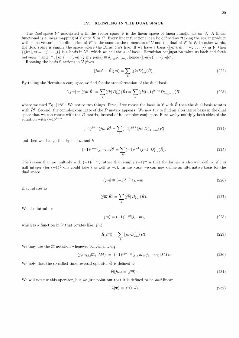
IV. ROTATING IN THE DUAL SPACE

The dual space V∗ associated with the vector space V is the linear space of linear functionals on V. A linearfunctional is a linear mapping of V onto R or C. Every linear functional can be defined as “taking the scalar productwith some vector”. The dimension of V∗ is the same as the dimension of V and the dual of V∗ is V. In other words,the dual space is simply the space where the Dirac bra’s live. If we have a basis {|jm〉,m = −j, . . . , j} in V, then{〈jm|,m = −j, . . . , j} is a basis in V∗, which we call the dual basis. Hermitian conjugation takes us back and forth

between V and V∗, |jm〉† = 〈jm|, 〈j1m1|j2m2〉 ≡ δj1j2δm1m2, hence (|jm〉c)† = 〈jm|c∗.

Rotating the basis functions in V gives

|jm〉′ ≡ R|jm〉 =∑k

|jk〉Djkm(R), (222)

By taking the Hermitian conjugate we find for the transformation of the dual basis

′〈jm| ≡ 〈jm|R† =∑k

〈jk|Dj,∗km(R) =

∑k

〈jk|(−1)k−mDj−k,−m(R) (223)

where we used Eq. (128). We notice two things. First, if we rotate the basis in V with R then the dual basis rotates

with R†. Second, the complex conjugate of the D matrix appears. We now try to find an alternative basis in the dualspace that we can rotate with the D-matrix, instead of its complex conjugate. First we by multiply both sides of theequation with (−1)j+m

(−1)j+m〈jm|R† =∑k

(−1)j+k〈jk|Dj−k,−m(R) (224)

and then we change the signs of m and k

(−1)j−m〈j,−m|R† =∑k

(−1)j−k〈j−k|Djkm(R). (225)

The reason that we multiply with (−1)j,−m, rather than simply (−1)m is that the former is also well defined if j is

half integer (for (−1)12 one could take i as well as −i). In any case, we can now define an alternative basis for the

dual space

〈jm| ≡ (−1)j−m〈j,−m| (226)

that rotates as

〈jm|R† =∑k

〈jk|Djkm(R). (227)

We also introduce

|jm〉 = (−1)j−m|j,−m〉, (228)

which is a function in V that rotates like |jm〉

R|jm〉 =∑k

|jk〉Djkm(R). (229)

We may use the m notation whenever convenient, e.g.

〈j1m1j2m2|JM〉 = (−1)j2−m2〈j1,m1, j2,−m2|JM〉. (230)

We note that the so called time reversal operator Θ is defined as

Θ|jm〉 = |jm〉. (231)

We will not use this operator, but we just point out that it is defined to be anti linear

Θλ|Ψ〉 ≡ λ∗Θ|Ψ〉. (232)

21

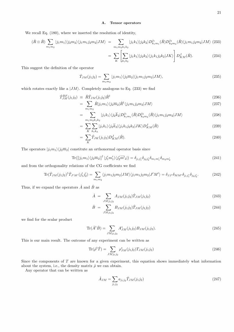
A. Tensor operators

We recall Eq. (180), where we inserted the resolution of identity,

(R⊗ R)∑m1m2

|j1m1〉|j2m2〉〈j1m1j2m2|JM〉 =∑

m1m2k1k2

|j1k1〉|j2k2〉Dj1k1m1

(R)Dj2k2m2

(R)〈j1m1j2m2|JM〉 (233)

=∑K

[∑k1k2

|j1k1〉|j2k2〉〈j1k1j2k2|JK〉

]DJKM (R). (234)

This suggest the definition of the operator

TJM (j1j2) =∑m1m2

|j1m1〉〈j2m2|〈j1m1j2m2|JM〉, (235)

which rotates exactly like a |JM〉. Completely analogous to Eq. (233) we find

TBFJM (j1j2) ≡ RTJM (j1j2)R† (236)

=∑m1m2

R|j1m1〉〈j2m2|R†〈j1m1j2m2|JM〉 (237)

=∑

m1m2k1k2

|j1k1〉〈j2k2|Dj1k1m1

(R)Dj2k2m2

(R)〈j1m1j2m2|JM〉 (238)

=∑K

∑k1k2

|j1k1〉〈j2k2|〈j1k1j2k2|JK〉DJKM (R) (239)

=∑K

TJK(j1j2)DJKM (R). (240)

The operators |j1m1〉〈j2m2| constitute an orthonormal operator basis since

Tr([|j1m1〉〈j2m2|]† |j′1m′1〉〈j′2m′2|) = δj1j′1δj2j′2δm1m′1δm2m′

2(241)

and from the orthogonality relations of the CG coefficients we find

Tr(TJM (j1j2)†TJ′M ′(j′1j′2) =

∑m1m2

〈j1m1j2m2|JM〉〈j1m1j2m2|J ′M ′〉 = δJJ ′δMM ′δj1j′1δj2j′2 . (242)

Thus, if we expand the operators A and B as

A =∑

JMj1j2

AJM (j1j2)TJM (j1j2) (243)

B =∑

JMj1j2

BJM (j1j2)TJM (j1j2) (244)

we find for the scalar product

Tr(A†B) =∑

JMj1j2

A∗JM (j1j2)BJM (j1j2). (245)

This is our main result. The outcome of any experiment can be written as

Tr(ρ†T ) =∑

JMj1j2

ρ∗JM (j1j2)TJM (j1j2) (246)

Since the components of T are known for a given experiment, this equation shows immediately what informationabout the system, i.e., the density matrix ρ we can obtain.

Any operator that can be written as

AJM =∑j1j2

aj1j2 TJM (j1j2) (247)

22

is called an irreducible tensor operator. It rotates like

RAJM R† =

∑K

AJKDJKM (R) (248)

and its matrix elements are

〈jm|AJM |jm′〉 = ajj′(√

2J + 1)(−1)j−m(

j J j′

−m M m′

)(249)

This result is known as the Wigner-Eckart theorem. The coefficient ajj′ is called the reduced matrix element and it

is often written as 〈j||A||j′〉.Gerrit C. Groenenboom, Nijmegen, November 1999

Appendix A: exercises

1. Derive the second equality sign in Eq. (22).

2. Show that N3 = −N (Eq. 41).

3. Do the summation in Eq. (44).

4. Show that e−iαp|x〉, is an eigenfunction of x, using only the definition x|x〉 = x|x〉 and the assumption that xand p are Hermitian operators with the commutation relation [x, p] = i. What is the eigenvalue?

5. Derive the following relations for the Levi-Civita tensor (Eq. 68)

eijkeij′k′ = δjj′δkk′ − δjk′δkj′ (250)

eijkeijk′ = 2δkk′ (251)

eijkeijk = 6, (252)

where we used Einstein summation convention: summation over repeated indices is implicit.

6. Show that

x× (y × z) = (x, z)y − (x,y)z. (253)

7. Using the last equation verify Eq. (64).

8. Derive Eq. (51). Hint: work out det(U [xyz]) in two ways, or use the Levi-Civita tensor.

9. Show that

B(t) = etABe−tA (254)

satisfies the equation

B(0) = B,d

dtB(t) = [A,B(t)] (255)

and therefore

B(t) = B +

∫ t

0

dτ [A,B(τ)]. (256)

Solve the last equation by iteration to derive Eq. (60)

10. Show that∑j1+j2J=|j1−j2|(2J + 1) = (2j1 + 1)(2j2 + 1). Hint: draw a grid of points (m1,m2) with mi = −ji . . . ji.

11. Compute the d12 (β) matrix [Eq. (121)].