animation & physically-based simulationdcor/graphics/cg-slides/graphics_tau_anim_pbs.pdf · 37...
TRANSCRIPT
1
Animation & Physically-Based Simulation
0368-3236, Spring 2019
Tel-Aviv University
Amit Bermano
2
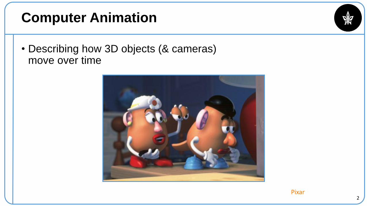
Computer Animation
• Describing how 3D objects (& cameras)move over time
Pixar
3
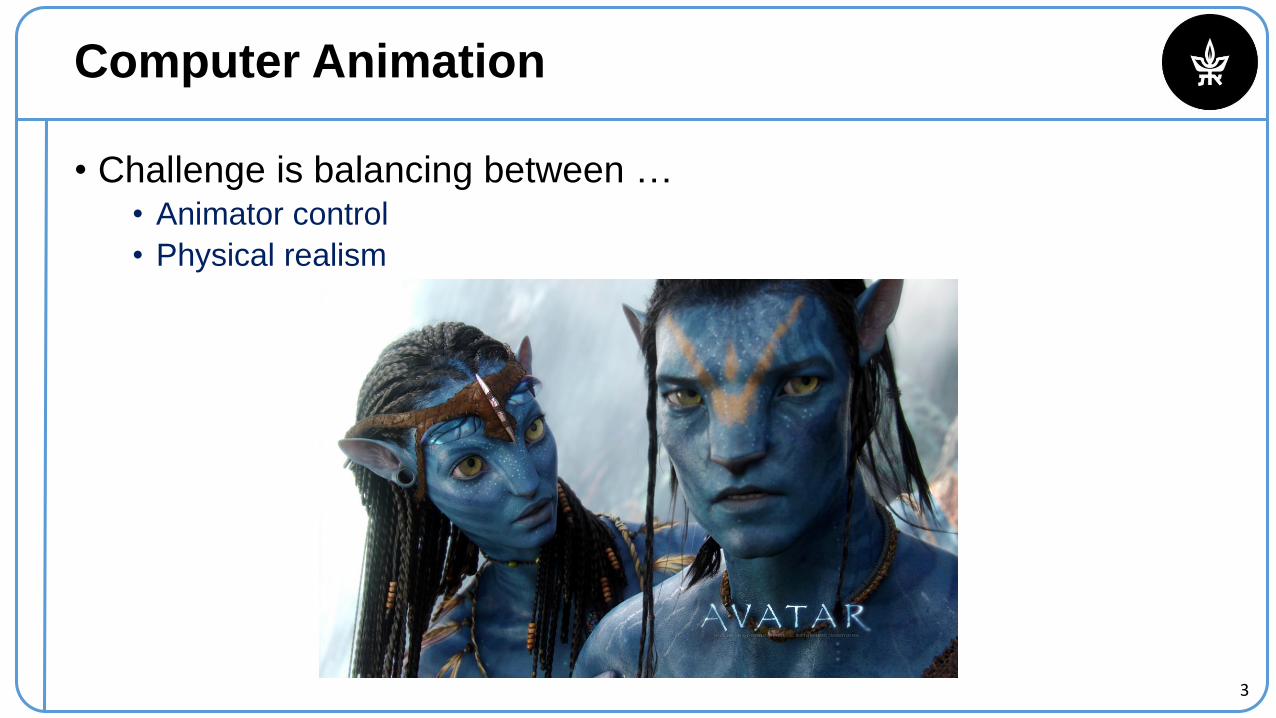
Computer Animation
• Challenge is balancing between …• Animator control
• Physical realism
4
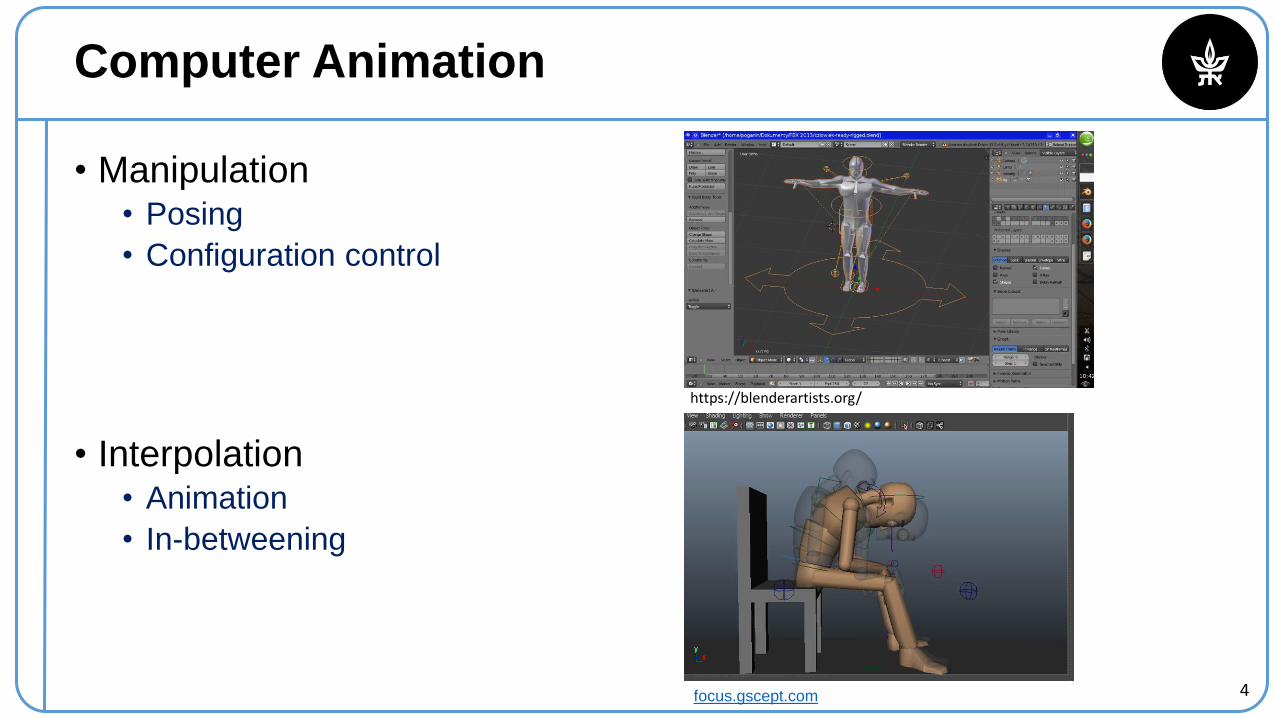
Computer Animation
• Manipulation• Posing
• Configuration control
• Interpolation• Animation
• In-betweening
focus.gscept.com
https://blenderartists.org/
5
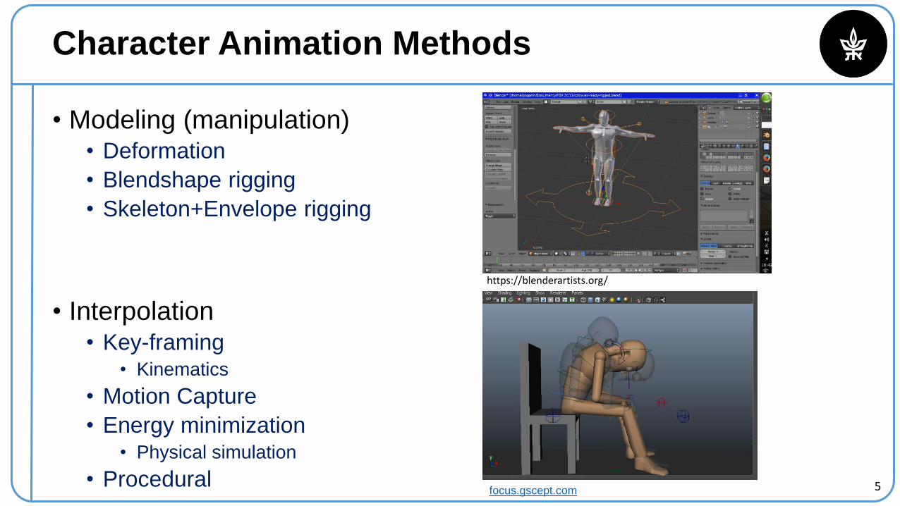
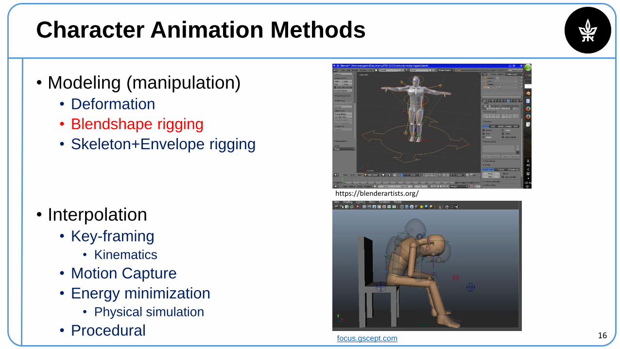
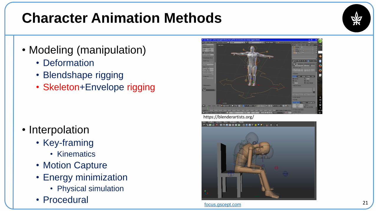
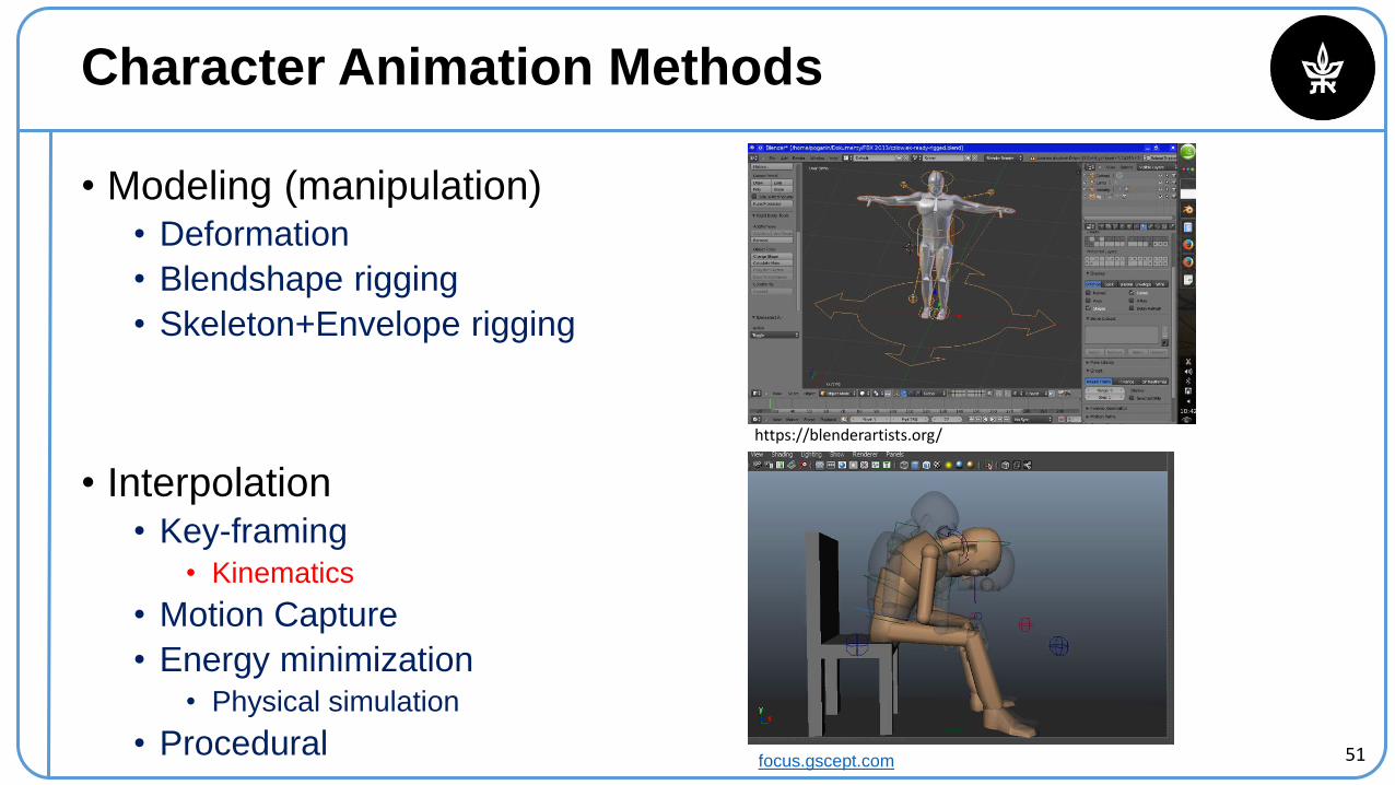
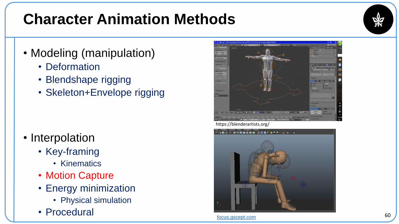
Character Animation Methods
• Modeling (manipulation)• Deformation
• Blendshape rigging
• Skeleton+Envelope rigging
• Interpolation• Key-framing
• Kinematics
• Motion Capture
• Energy minimization• Physical simulation
• Proceduralfocus.gscept.com
https://blenderartists.org/
6
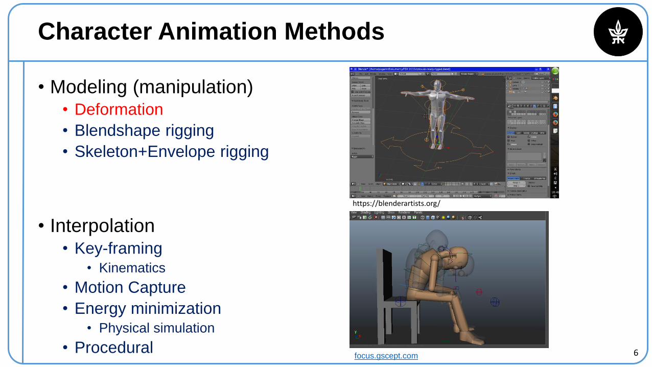
Character Animation Methods
• Modeling (manipulation)• Deformation
• Blendshape rigging
• Skeleton+Envelope rigging
• Interpolation• Key-framing
• Kinematics
• Motion Capture
• Energy minimization• Physical simulation
• Proceduralfocus.gscept.com
https://blenderartists.org/
7
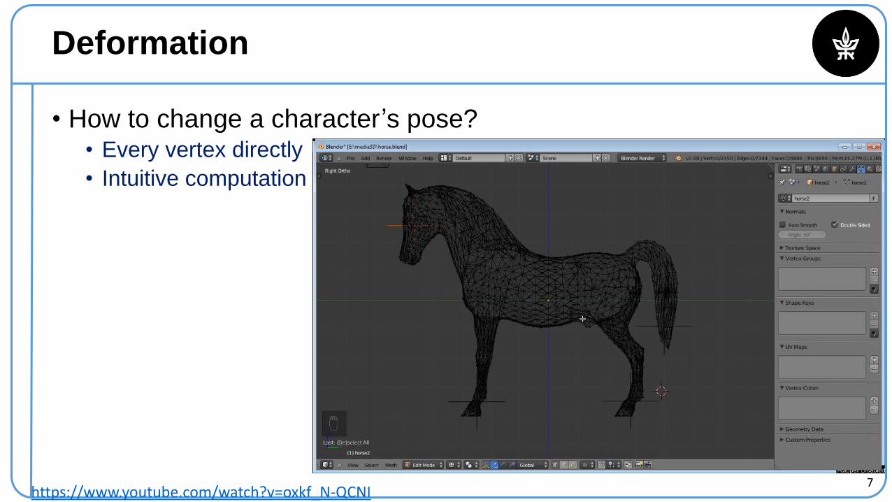
Deformation
• How to change a character’s pose?• Every vertex directly
• Intuitive computation
https://www.youtube.com/watch?v=oxkf_N-QCNI
8
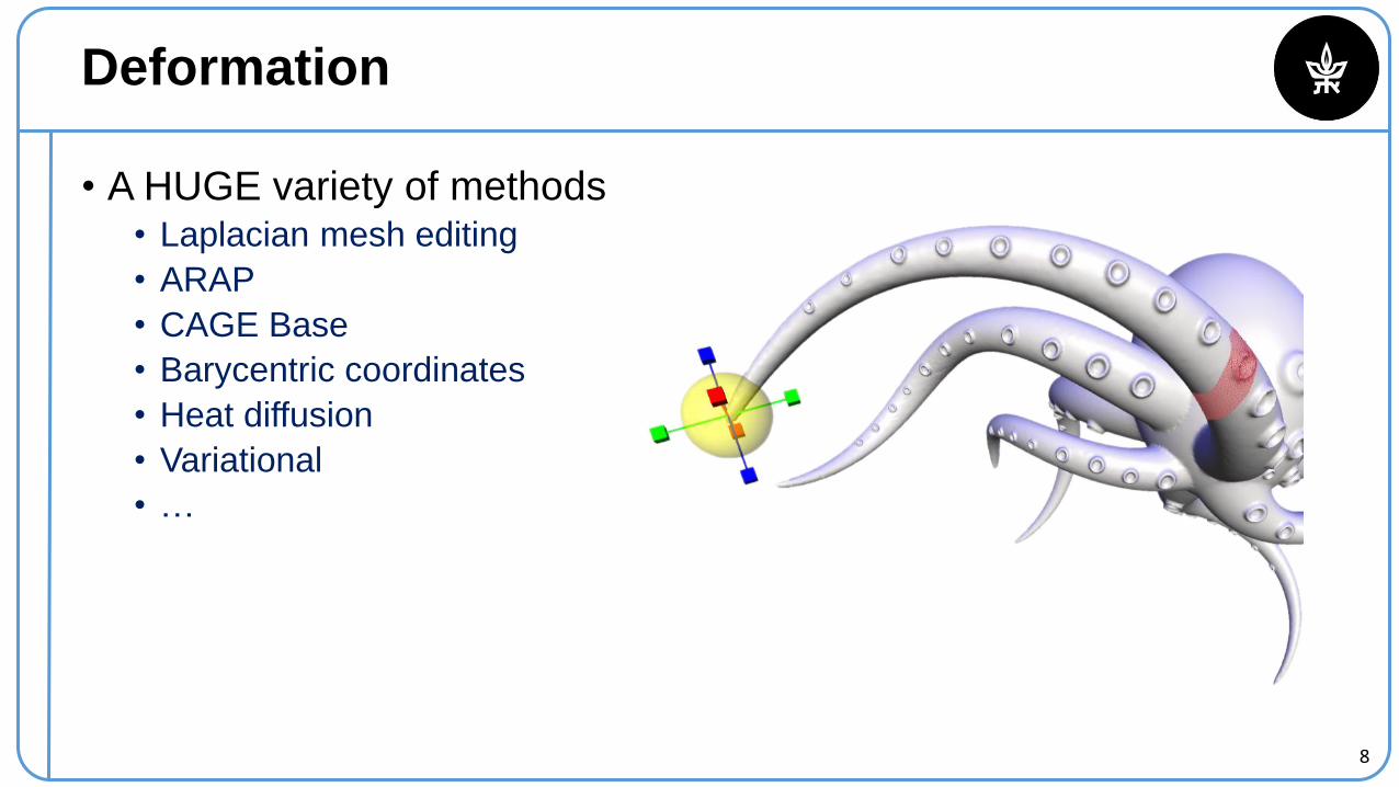
Deformation
• A HUGE variety of methods• Laplacian mesh editing
• ARAP
• CAGE Base
• Barycentric coordinates
• Heat diffusion
• Variational
• …
9
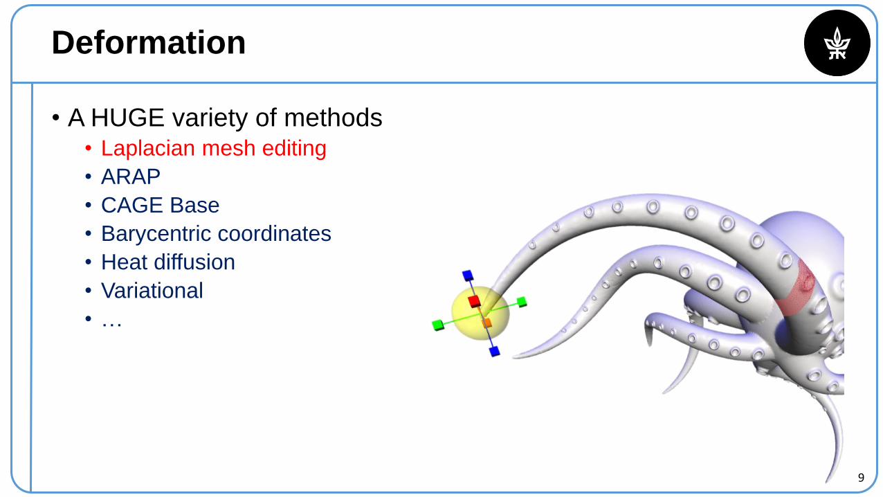
Deformation
• A HUGE variety of methods• Laplacian mesh editing
• ARAP
• CAGE Base
• Barycentric coordinates
• Heat diffusion
• Variational
• …
10
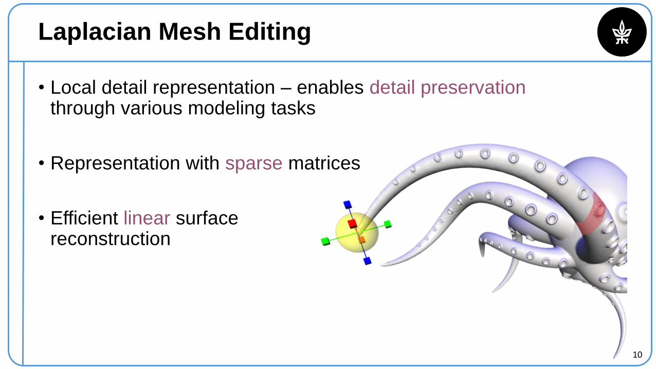
Laplacian Mesh Editing
• Local detail representation – enables detail preservationthrough various modeling tasks
• Representation with sparse matrices
• Efficient linear surface reconstruction
11
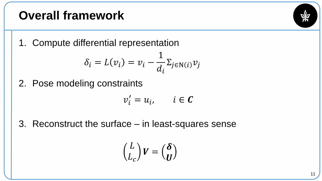
Overall framework
1. Compute differential representation
2. Pose modeling constraints
3. Reconstruct the surface – in least-squares sense
𝛿𝑖 = 𝐿 𝑣𝑖 = 𝑣𝑖 −1
𝑑𝑖Σ𝑗∈N 𝑖 𝑣𝑗
𝑣𝑖′ = 𝑢𝑖 , 𝑖 ∈ 𝑪
𝐿𝐿𝑐
𝑽 =𝜹𝑼
12
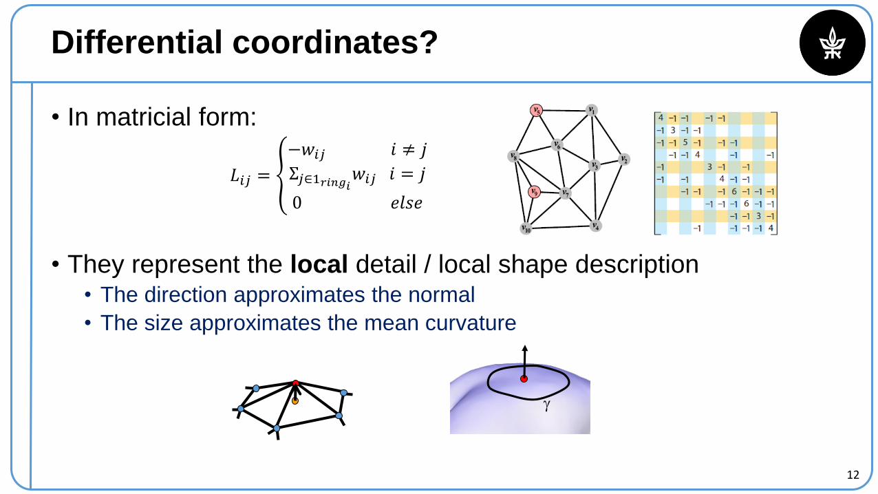
Differential coordinates?
• In matricial form:
• They represent the local detail / local shape description• The direction approximates the normal
• The size approximates the mean curvature
𝐿𝑖𝑗 = ൞
−𝑤𝑖𝑗 𝑖 ≠ 𝑗
Σ𝑗∈1𝑟𝑖𝑛𝑔𝑖𝑤𝑖𝑗 𝑖 = 𝑗
0 𝑒𝑙𝑠𝑒
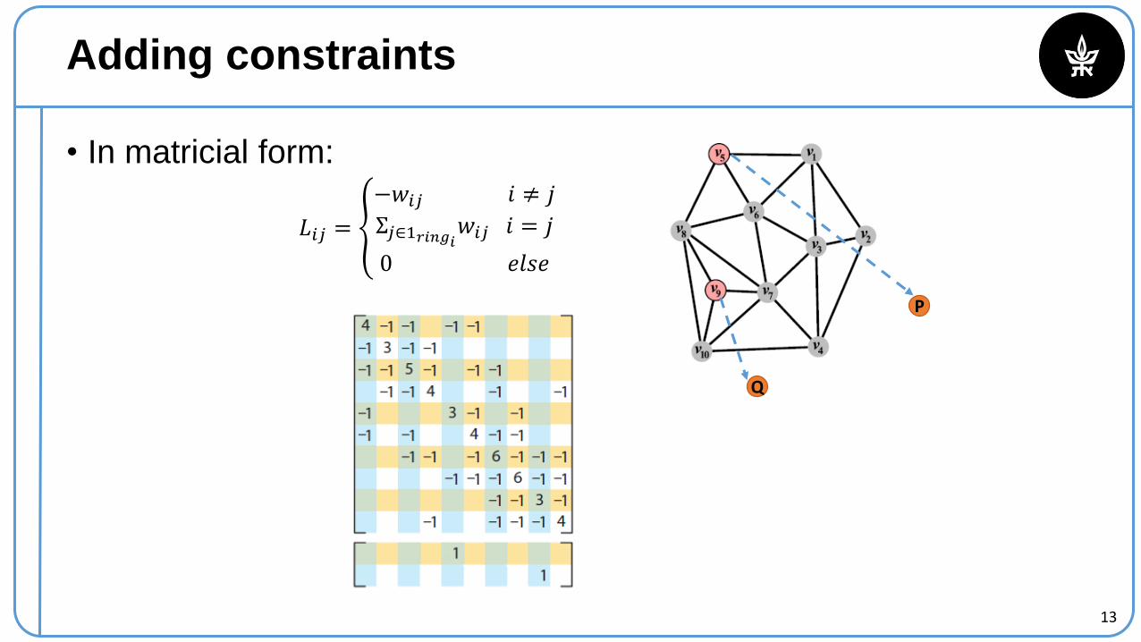
13
• In matricial form:
𝐿𝑖𝑗 = ൞
−𝑤𝑖𝑗 𝑖 ≠ 𝑗
Σ𝑗∈1𝑟𝑖𝑛𝑔𝑖𝑤𝑖𝑗 𝑖 = 𝑗
0 𝑒𝑙𝑠𝑒
P
Q
Adding constraints
14
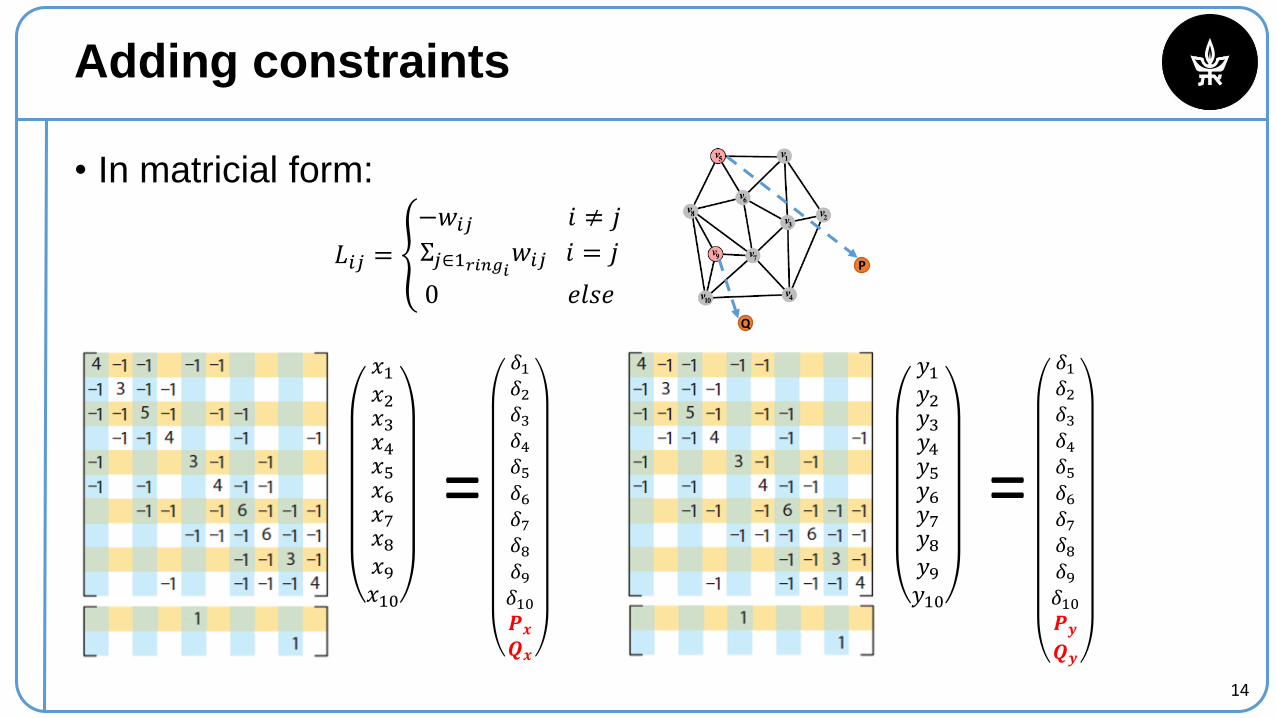
Adding constraints
• In matricial form:
𝐿𝑖𝑗 = ൞
−𝑤𝑖𝑗 𝑖 ≠ 𝑗
Σ𝑗∈1𝑟𝑖𝑛𝑔𝑖𝑤𝑖𝑗 𝑖 = 𝑗
0 𝑒𝑙𝑠𝑒
𝑥1𝑥2𝑥3𝑥4𝑥5𝑥6𝑥7𝑥8𝑥9𝑥10
=
𝛿1𝛿2𝛿3𝛿4𝛿5𝛿6𝛿7𝛿8𝛿9𝛿10𝑷𝒙
𝑸𝒙
𝑦1𝑦2𝑦3𝑦4𝑦5𝑦6𝑦7𝑦8𝑦9𝑦10
=
𝛿1𝛿2𝛿3𝛿4𝛿5𝛿6𝛿7𝛿8𝛿9𝛿10𝑷𝒚
𝑸𝒚
P
Q
15
Demo
16
Character Animation Methods
• Modeling (manipulation)• Deformation
• Blendshape rigging
• Skeleton+Envelope rigging
• Interpolation• Key-framing
• Kinematics
• Motion Capture
• Energy minimization• Physical simulation
• Proceduralfocus.gscept.com
https://blenderartists.org/
17
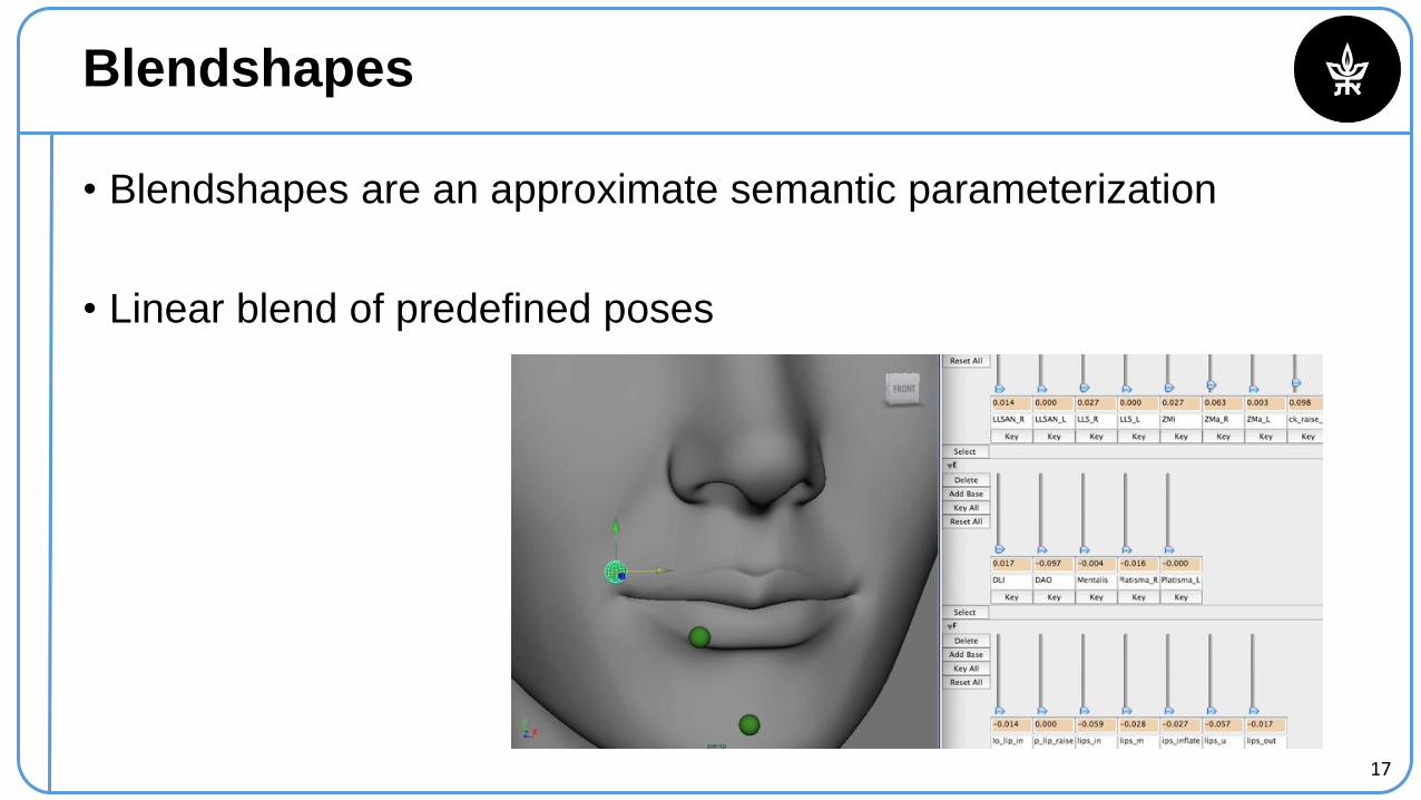
Blendshapes
• Blendshapes are an approximate semantic parameterization
• Linear blend of predefined poses
18
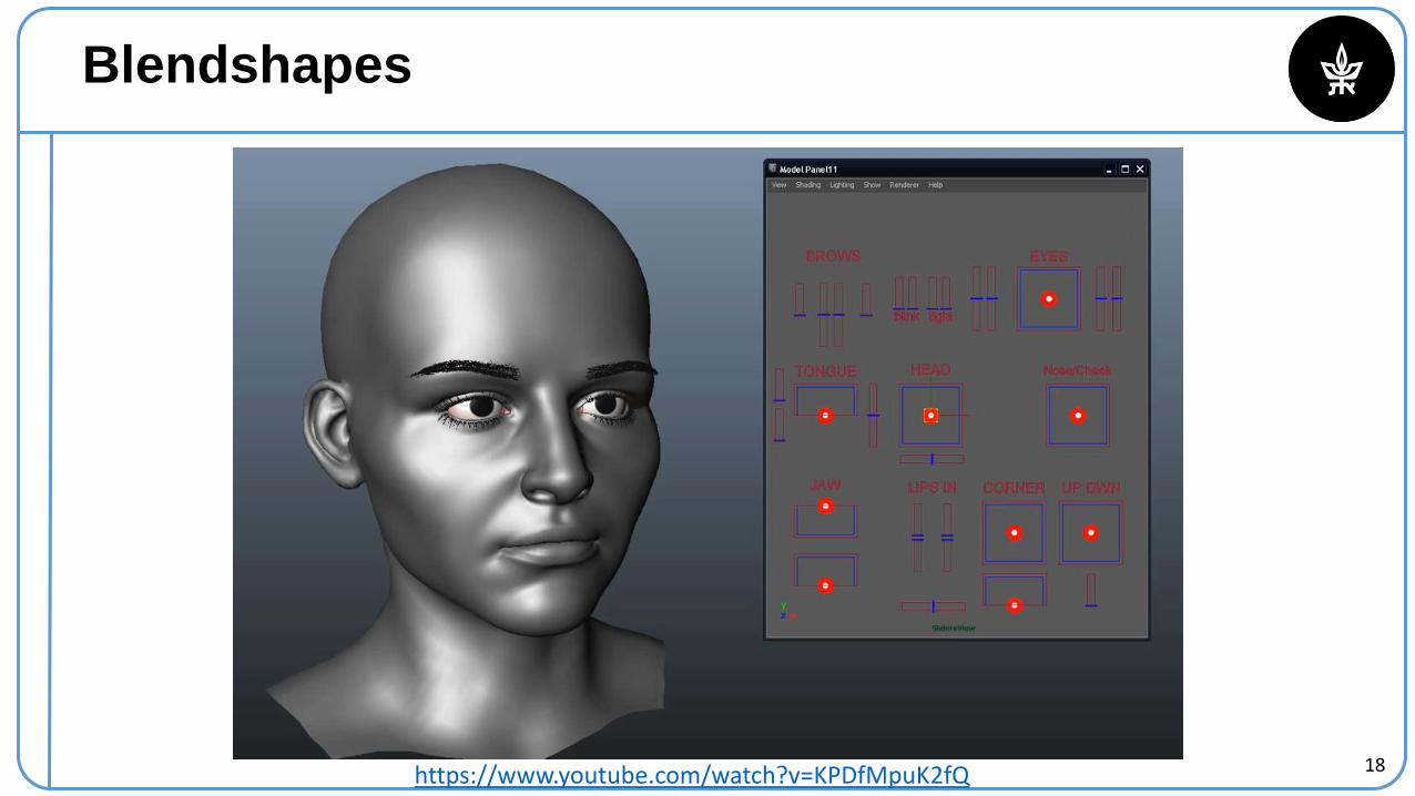
Blendshapes
https://www.youtube.com/watch?v=KPDfMpuK2fQ
19
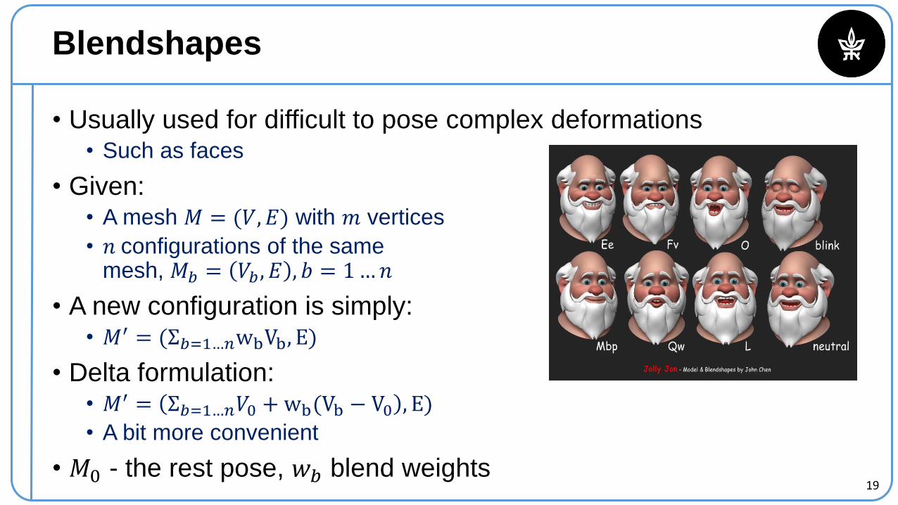
Blendshapes
• Usually used for difficult to pose complex deformations• Such as faces
• Given: • A mesh 𝑀 = (𝑉, 𝐸) with 𝑚 vertices
• 𝑛 configurations of the samemesh, 𝑀𝑏 = 𝑉𝑏 , 𝐸 , 𝑏 = 1…𝑛
• A new configuration is simply:• 𝑀′ = (Σ𝑏=1…𝑛wbVb, E)
• Delta formulation:• 𝑀′ = Σ𝑏=1…𝑛𝑉0 +wb(Vb − V0 , E)
• A bit more convenient
• 𝑀0 - the rest pose, 𝑤𝑏 blend weights
20
Blendshapes
https://www.youtube.com/watch?v=jBOEzXYMugE
21
Character Animation Methods
• Modeling (manipulation)• Deformation
• Blendshape rigging
• Skeleton+Envelope rigging
• Interpolation• Key-framing
• Kinematics
• Motion Capture
• Energy minimization• Physical simulation
• Proceduralfocus.gscept.com
https://blenderartists.org/
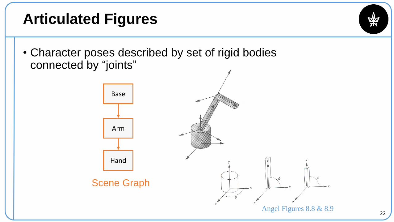
22Angel Figures 8.8 & 8.9
Base
Arm
Hand
Scene Graph
Articulated Figures
• Character poses described by set of rigid bodies connected by “joints”
23
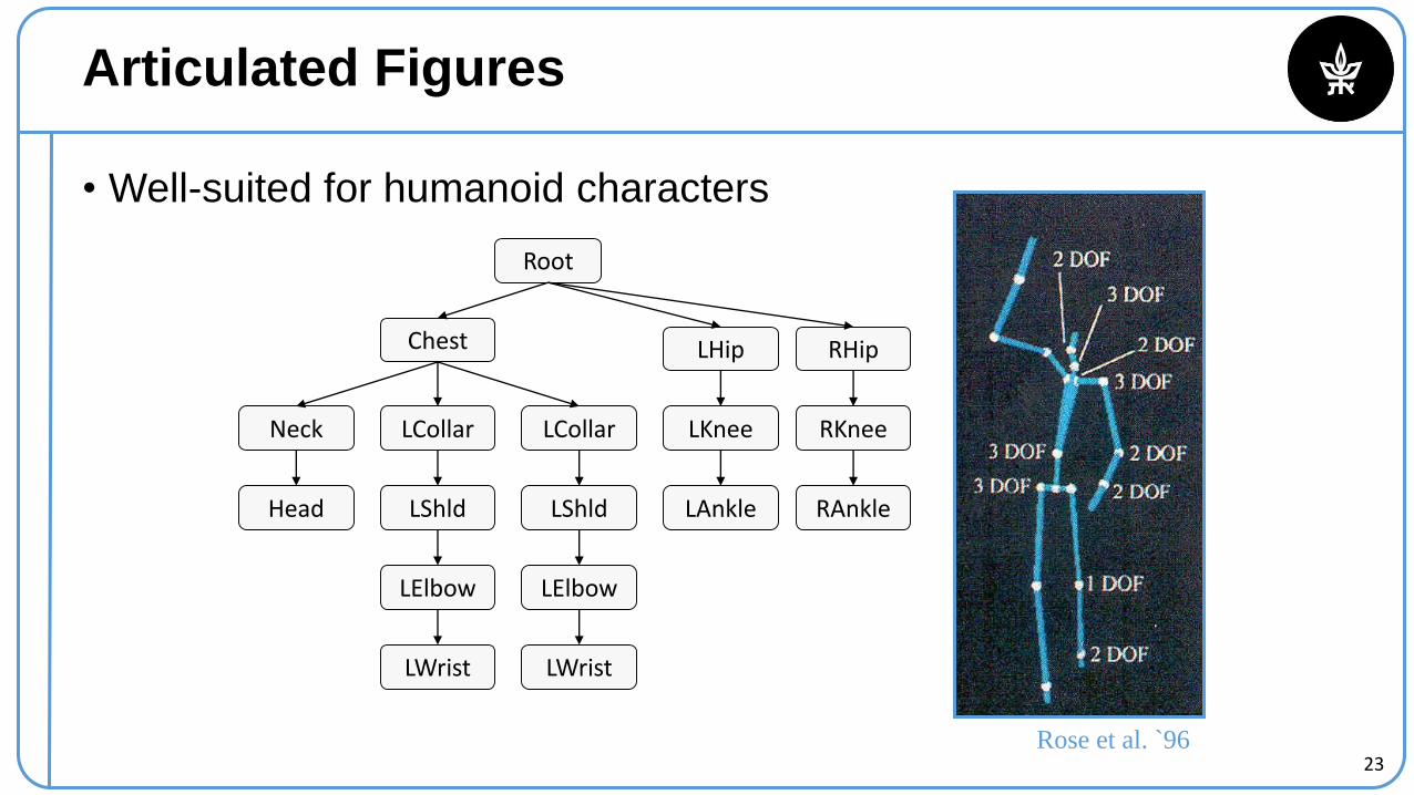
Articulated Figures
• Well-suited for humanoid characters
Rose et al. `96
Root
LHip
LKnee
LAnkle
RHip
RKnee
RAnkle
Chest
LCollar
LShld
LElbow
LWrist
LCollar
LShld
LElbow
LWrist
Neck
Head
25
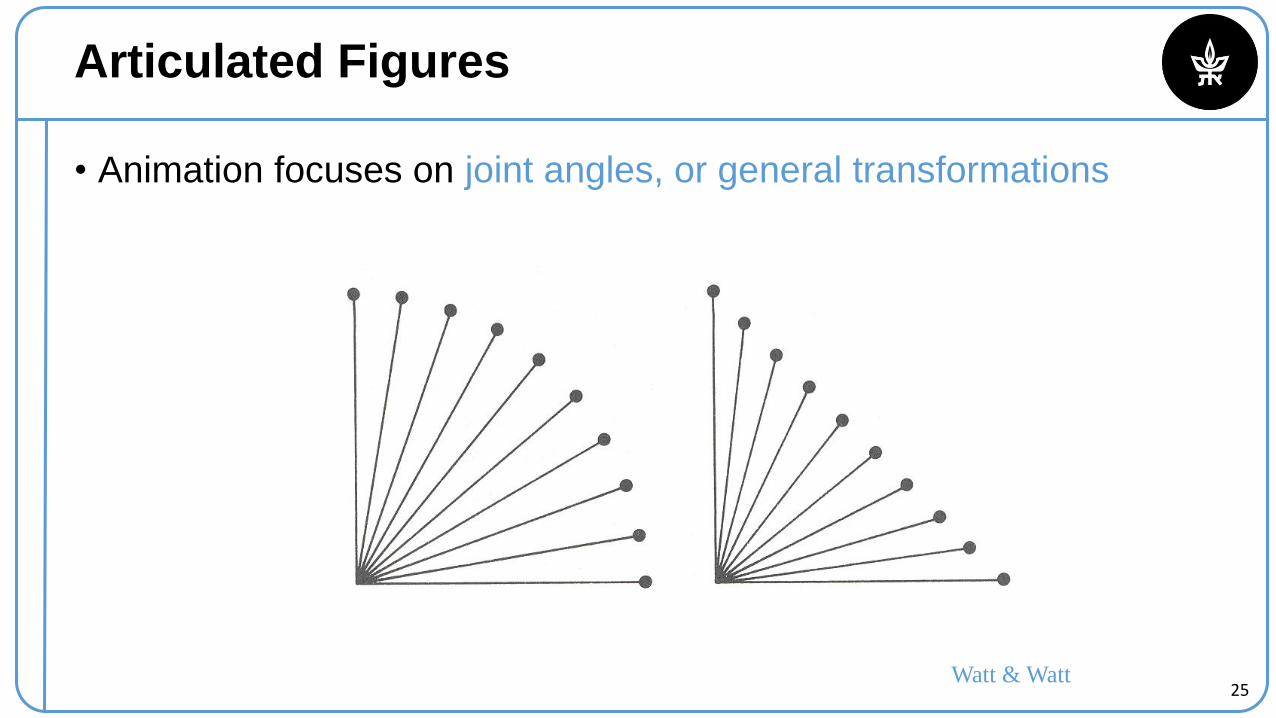
Articulated Figures
• Animation focuses on joint angles, or general transformations
Watt & Watt
26
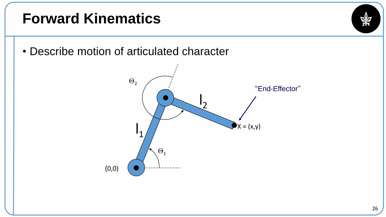
Forward Kinematics
• Describe motion of articulated character
1
2
X = (x,y)
l2
l1
(0,0)
“End-Effector”
27
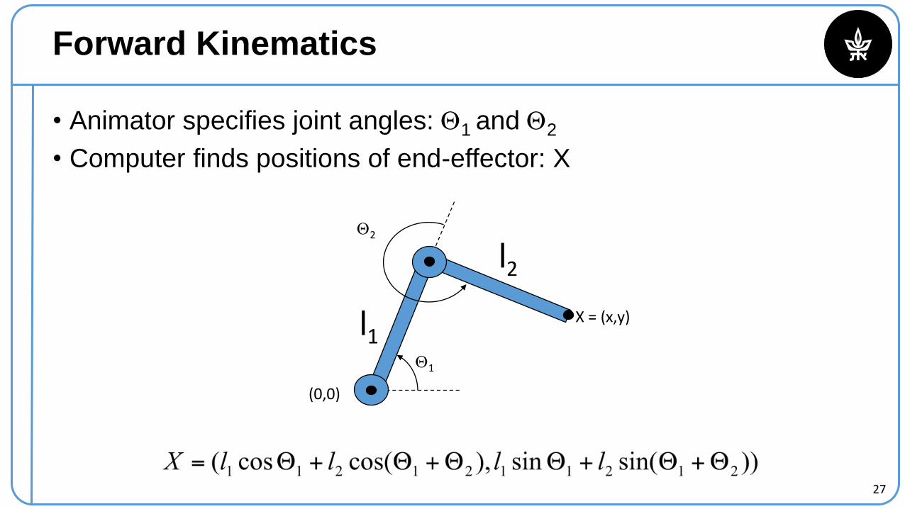
Forward Kinematics
• Animator specifies joint angles: 1 and 2
• Computer finds positions of end-effector: X
1
2
X = (x,y)
l2
l1
(0,0)
29
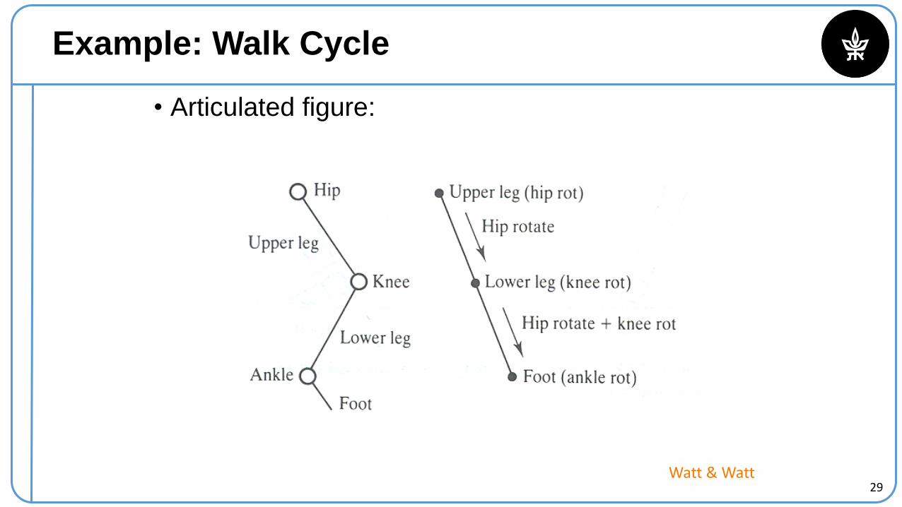
Example: Walk Cycle
• Articulated figure:
Watt & Watt
30
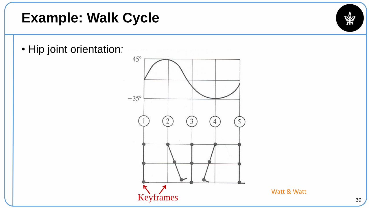
Example: Walk Cycle
• Hip joint orientation:
Watt & Watt Keyframes
31
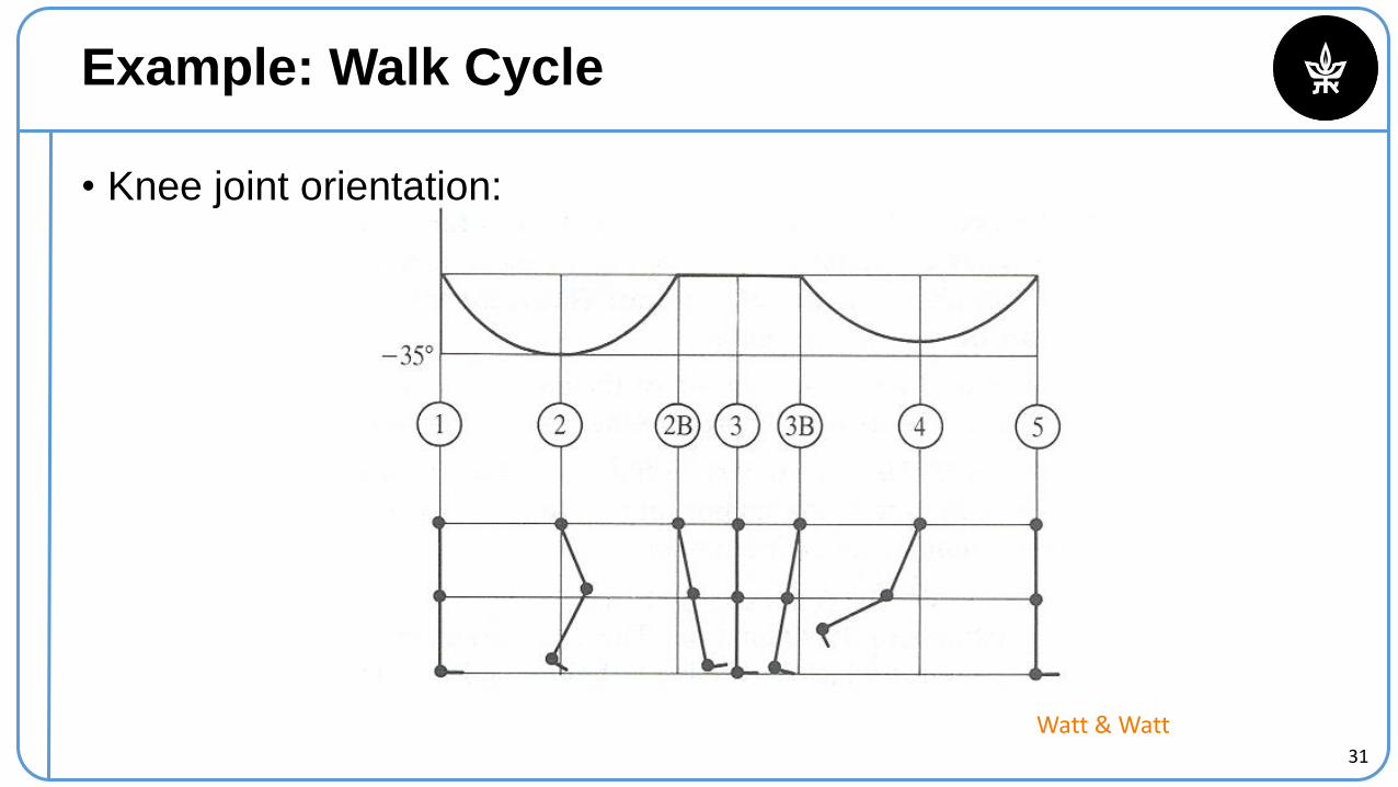
Example: Walk Cycle
• Knee joint orientation:
Watt & Watt
32
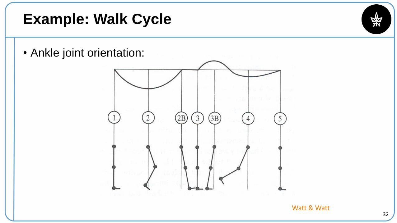
Example: Walk Cycle
• Ankle joint orientation:
Watt & Watt
33
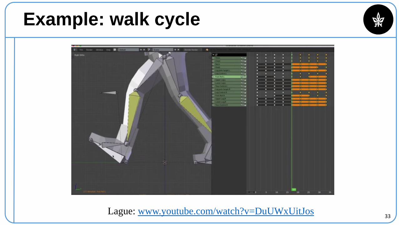
Example: walk cycle
Lague: www.youtube.com/watch?v=DuUWxUitJos

34
Character Animation Methods
• Modeling (manipulation)• Deformation
• Blendshape rigging
• Skeleton+Envelope rigging
• Interpolation• Key-framing
• Kinematics
• Motion Capture
• Energy minimization• Physical simulation
• Proceduralfocus.gscept.com
https://blenderartists.org/
35
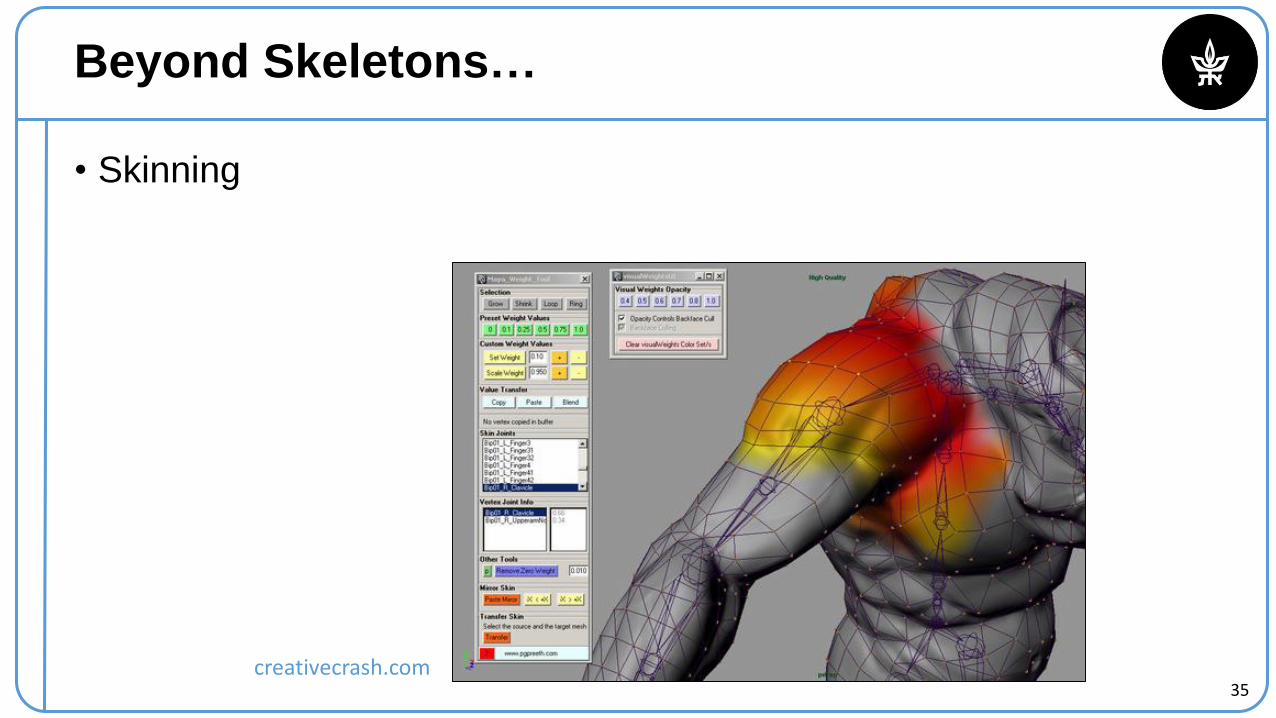
Beyond Skeletons…
• Skinning
creativecrash.com
36
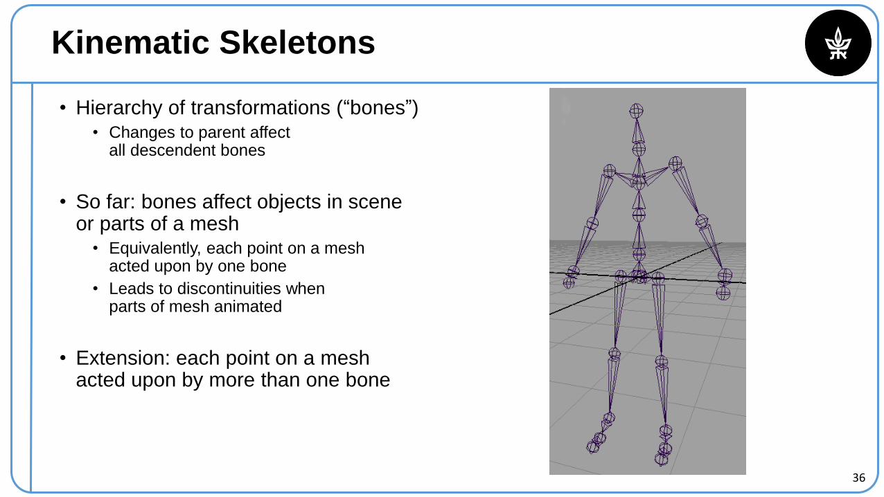
Kinematic Skeletons
• Hierarchy of transformations (“bones”)• Changes to parent affect
all descendent bones
• So far: bones affect objects in sceneor parts of a mesh
• Equivalently, each point on a meshacted upon by one bone
• Leads to discontinuities whenparts of mesh animated
• Extension: each point on a meshacted upon by more than one bone
37
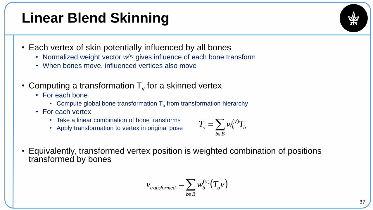
Linear Blend Skinning
• Each vertex of skin potentially influenced by all bones• Normalized weight vector w(v) gives influence of each bone transform
• When bones move, influenced vertices also move
• Computing a transformation Tv for a skinned vertex• For each bone
• Compute global bone transformation Tb from transformation hierarchy
• For each vertex• Take a linear combination of bone transforms
• Apply transformation to vertex in original pose
• Equivalently, transformed vertex position is weighted combination of positions transformed by bones
Bb
b
v
bv TwT )(
Bb
b
v
bdtransforme vTwv )(
38
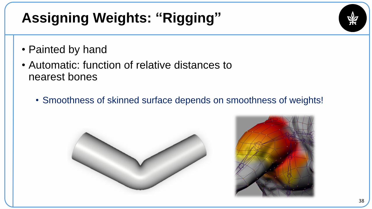
Assigning Weights: “Rigging”
• Painted by hand
• Automatic: function of relative distances tonearest bones
• Smoothness of skinned surface depends on smoothness of weights!
39
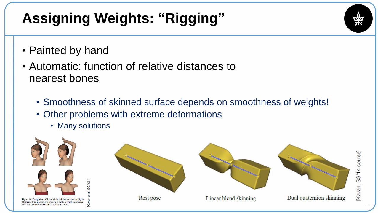
Assigning Weights: “Rigging”
• Painted by hand
• Automatic: function of relative distances tonearest bones
• Smoothness of skinned surface depends on smoothness of weights!
• Other problems with extreme deformations• Many solutions
40
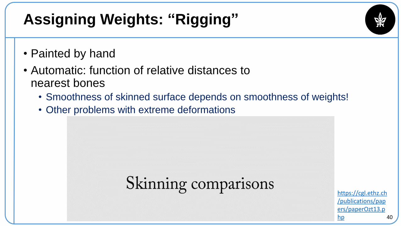
Assigning Weights: “Rigging”
• Painted by hand
• Automatic: function of relative distances tonearest bones
• Smoothness of skinned surface depends on smoothness of weights!
• Other problems with extreme deformations
https://cgl.ethz.ch/publications/papers/paperOzt13.php
41
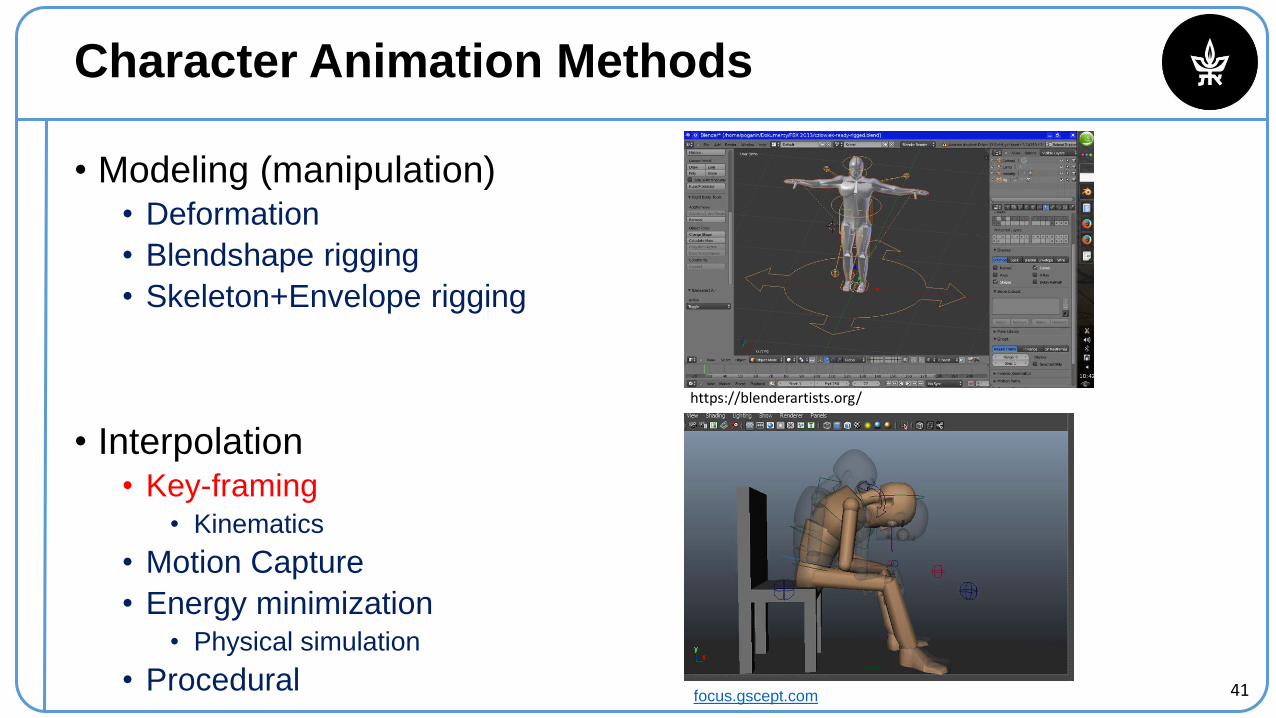
Character Animation Methods
• Modeling (manipulation)• Deformation
• Blendshape rigging
• Skeleton+Envelope rigging
• Interpolation• Key-framing
• Kinematics
• Motion Capture
• Energy minimization• Physical simulation
• Proceduralfocus.gscept.com
https://blenderartists.org/
42
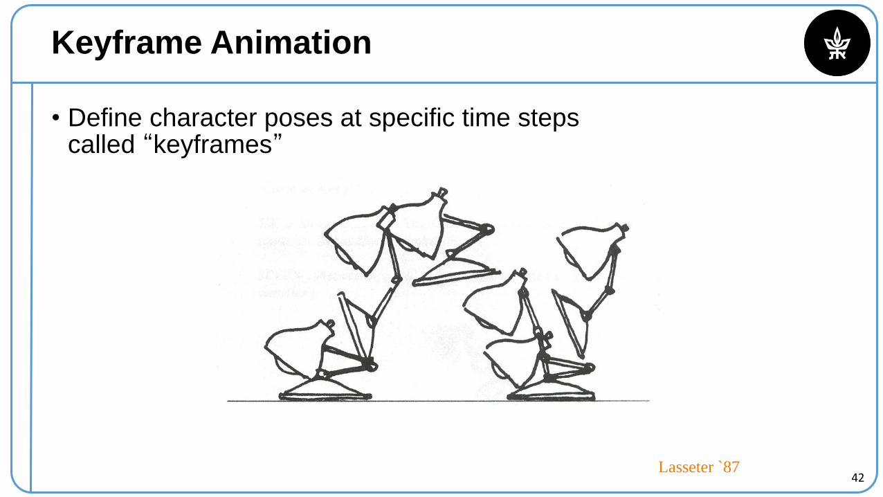
Keyframe Animation
• Define character poses at specific time stepscalled “keyframes”
Lasseter `87
43
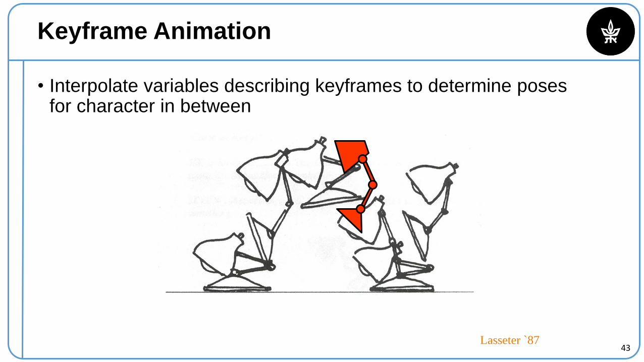
Keyframe Animation
• Interpolate variables describing keyframes to determine poses for character in between
Lasseter `87
44
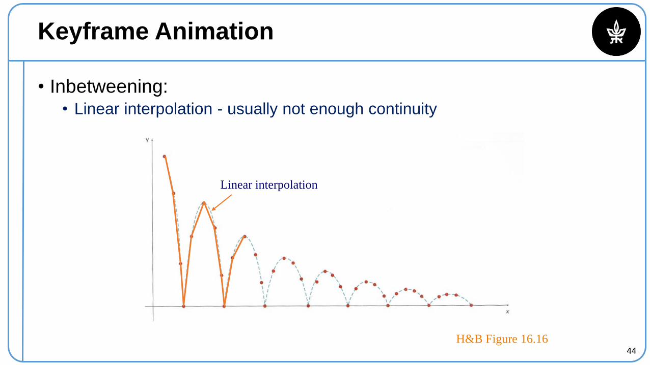
Keyframe Animation
• Inbetweening:• Linear interpolation - usually not enough continuity
H&B Figure 16.16
Linear interpolation
45
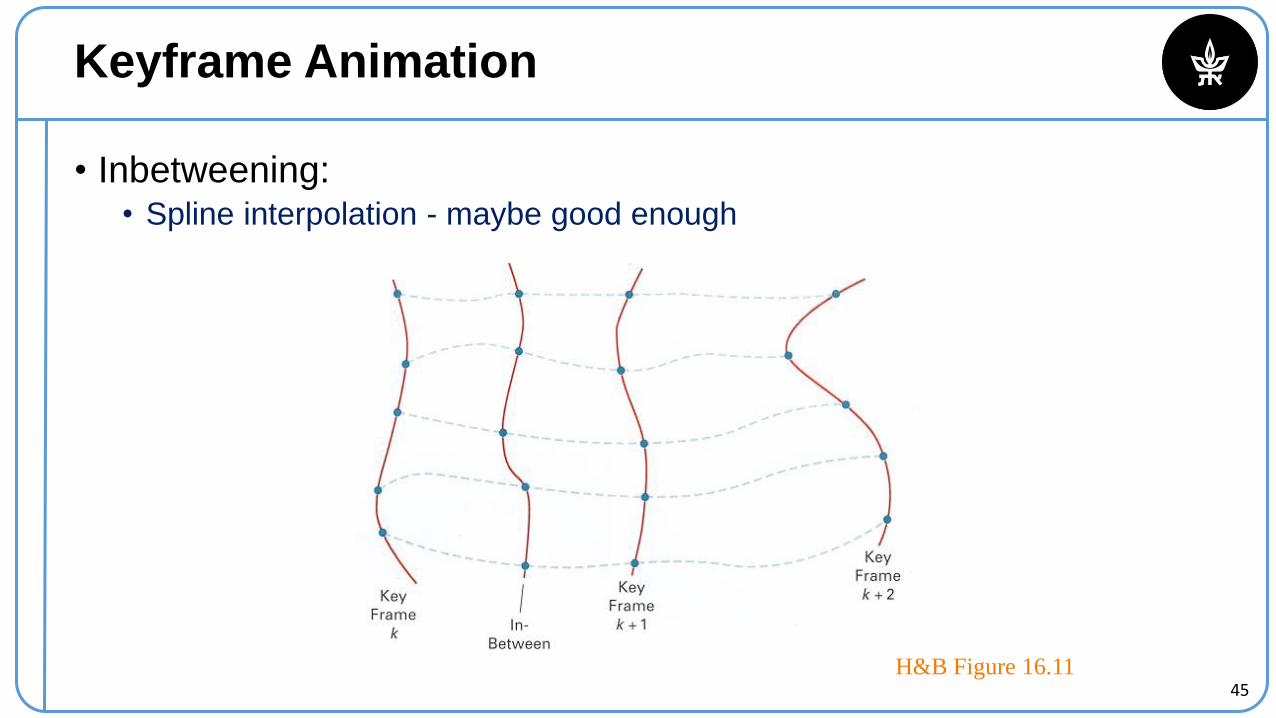
Keyframe Animation
• Inbetweening:• Spline interpolation - maybe good enough
H&B Figure 16.11
46
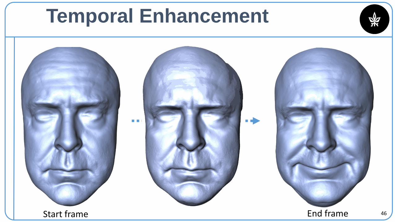
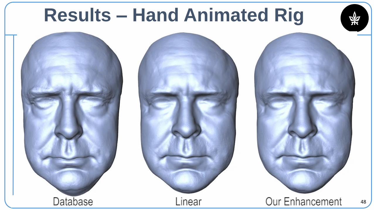
Temporal Enhancement
Start frame End frame
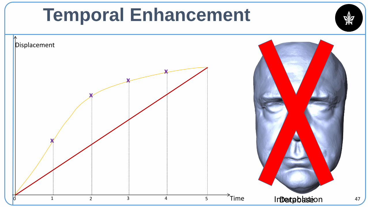
47Time0 1 2 3 4 5
Displacement
Temporal Enhancement
xx
x
x
DatabaseInterpolation
48
Results – Hand Animated Rig
50
Example: Ball Boy
Fujito, Milliron, Ngan, & Sanocki
Princeton University
“Ballboy”
51
Character Animation Methods
• Modeling (manipulation)• Deformation
• Blendshape rigging
• Skeleton+Envelope rigging
• Interpolation• Key-framing
• Kinematics
• Motion Capture
• Energy minimization• Physical simulation
• Proceduralfocus.gscept.com
https://blenderartists.org/
53
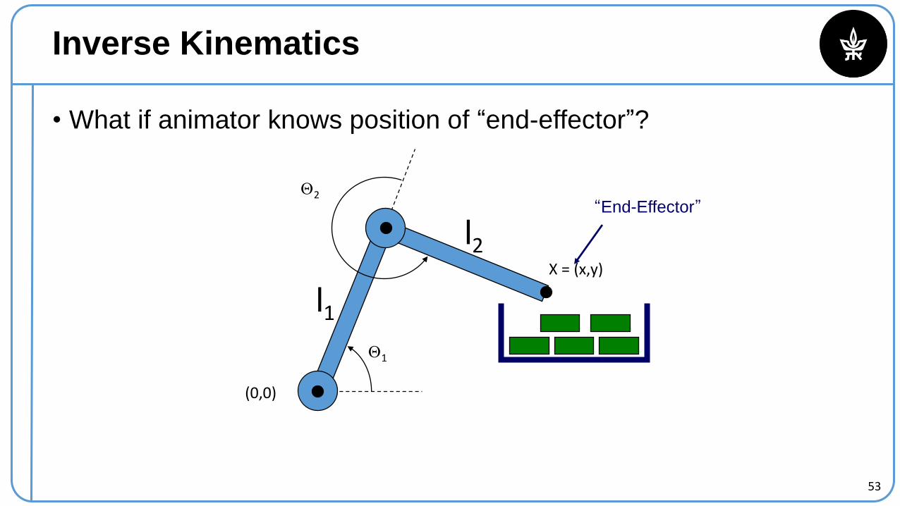
Inverse Kinematics
• What if animator knows position of “end-effector”?
1
2
X = (x,y)
l2
l1
(0,0)
“End-Effector”
54
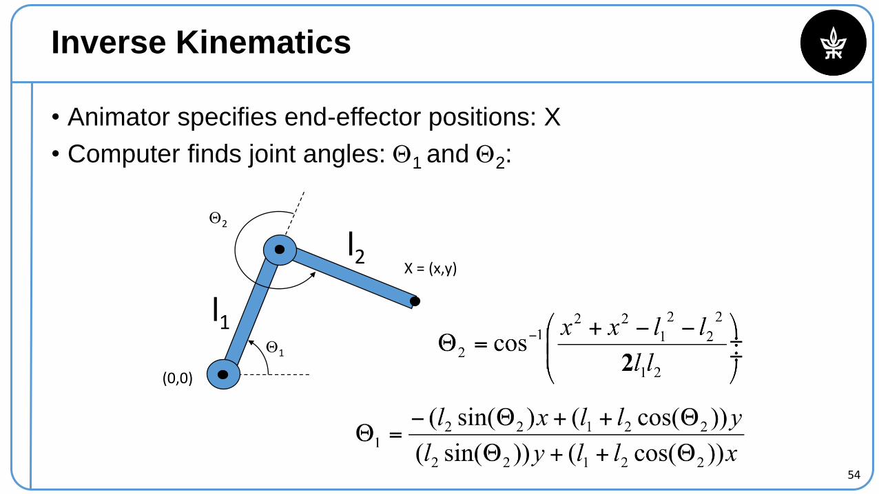
Inverse Kinematics
• Animator specifies end-effector positions: X
• Computer finds joint angles: 1 and 2:
1
2
X = (x,y)l2
l1
(0,0)
55
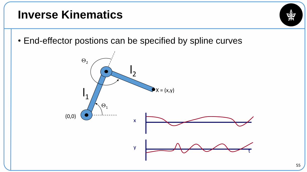
Inverse Kinematics
• End-effector postions can be specified by spline curves
1
2
X = (x,y)
l2
l1
(0,0)
y
x
t
56
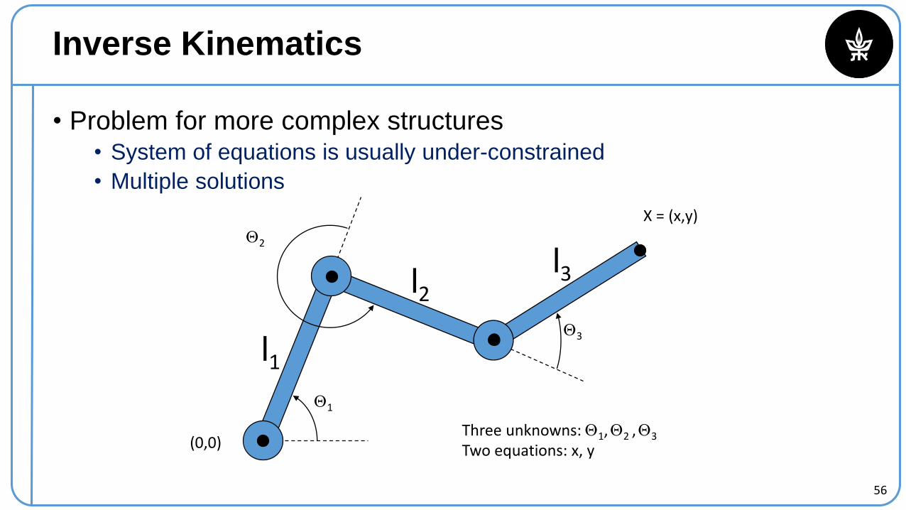
Inverse Kinematics
• Problem for more complex structures• System of equations is usually under-constrained
• Multiple solutions
1
2
l2
l1
(0,0)
X = (x,y)
l3
3
Three unknowns: 1,2 ,3
Two equations: x, y
57
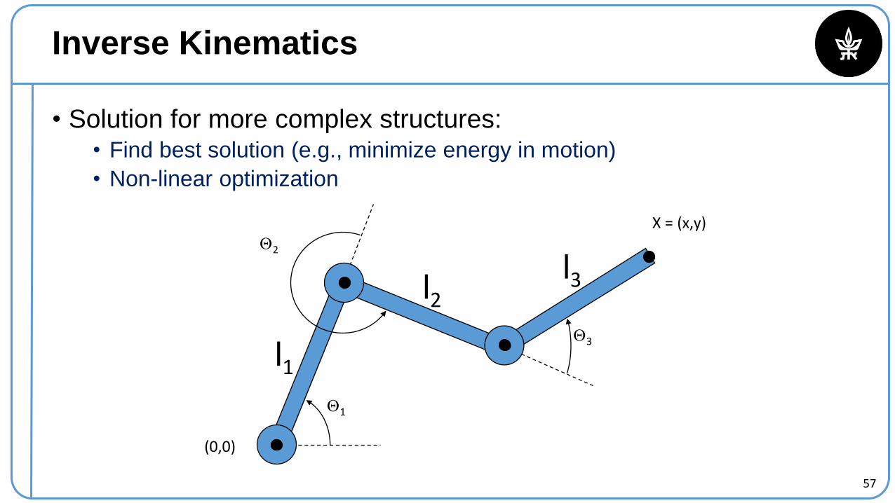
Inverse Kinematics
• Solution for more complex structures:• Find best solution (e.g., minimize energy in motion)
• Non-linear optimization
1
2
l2
l1
(0,0)
X = (x,y)
l3
3
58
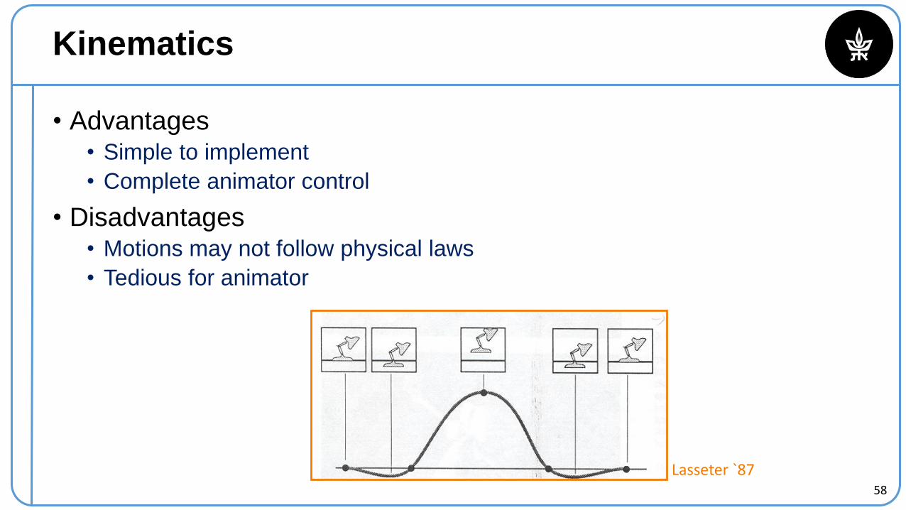
Kinematics
• Advantages• Simple to implement
• Complete animator control
• Disadvantages• Motions may not follow physical laws
• Tedious for animator
Lasseter `87
59
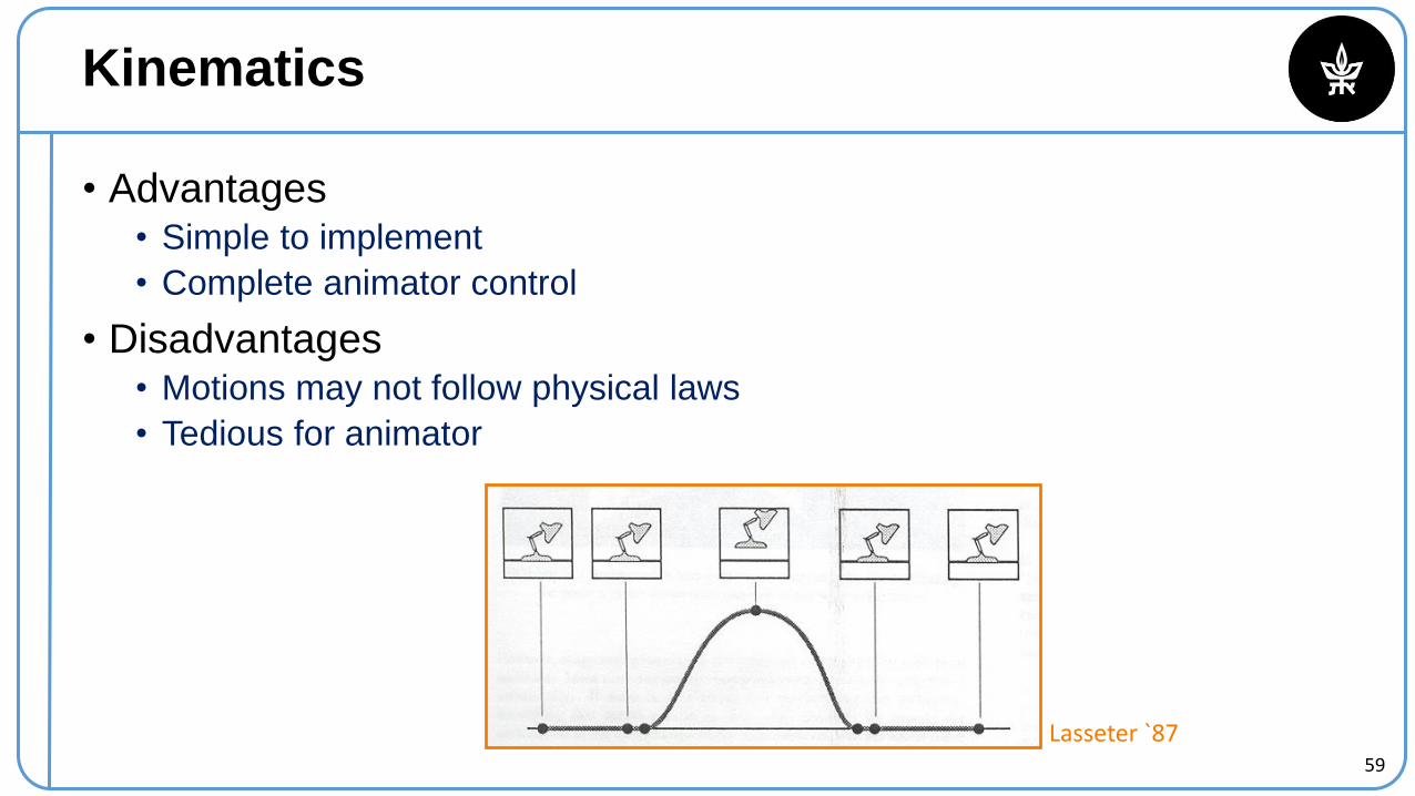
Kinematics
• Advantages• Simple to implement
• Complete animator control
• Disadvantages• Motions may not follow physical laws
• Tedious for animator
Lasseter `87
60
Character Animation Methods
• Modeling (manipulation)• Deformation
• Blendshape rigging
• Skeleton+Envelope rigging
• Interpolation• Key-framing
• Kinematics
• Motion Capture
• Energy minimization• Physical simulation
• Proceduralfocus.gscept.com
https://blenderartists.org/
61
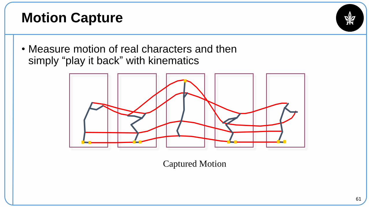
Motion Capture
• Measure motion of real characters and thensimply “play it back” with kinematics
Captured Motion
62
Motion Capture
• Measure motion of real characters and then simply “play it back” with kinematics
https://www.youtube.com/watch?v=MVvDw15-3e8
63
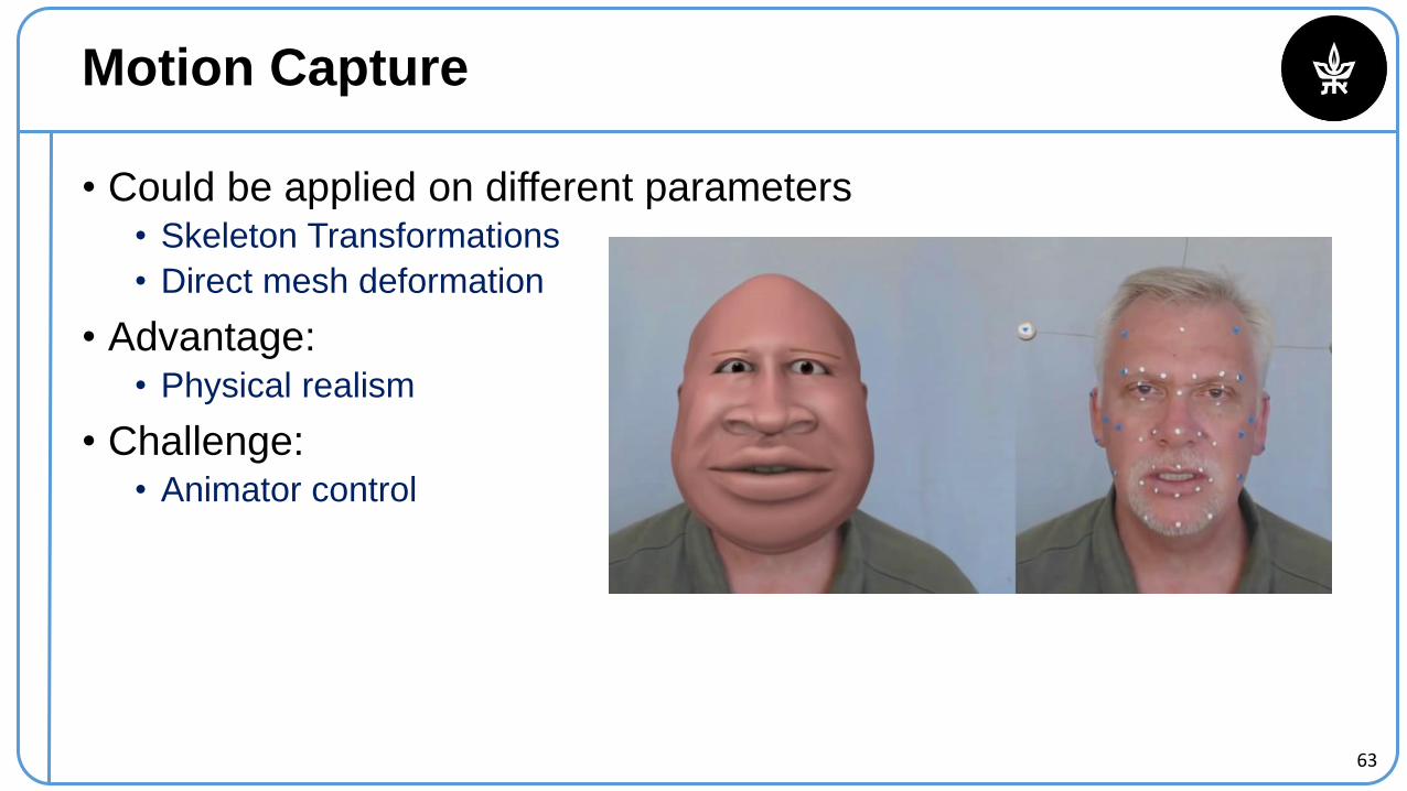
Motion Capture
• Could be applied on different parameters• Skeleton Transformations
• Direct mesh deformation
• Advantage:• Physical realism
• Challenge:• Animator control
65
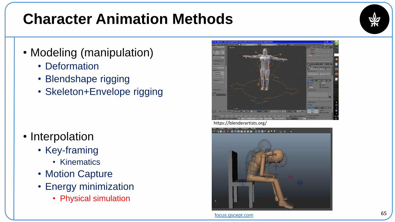
Character Animation Methods
• Modeling (manipulation)• Deformation
• Blendshape rigging
• Skeleton+Envelope rigging
• Interpolation• Key-framing
• Kinematics
• Motion Capture
• Energy minimization• Physical simulation
focus.gscept.com
https://blenderartists.org/
66
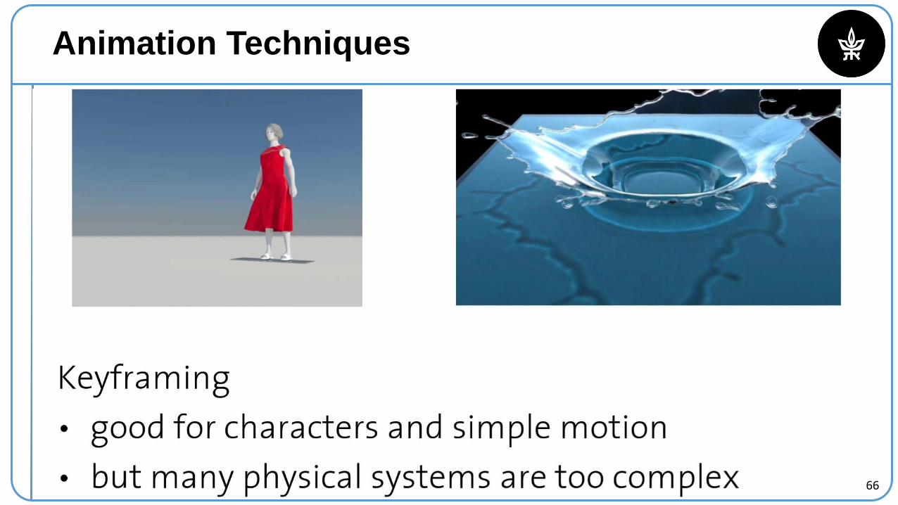
Animation Techniques
67
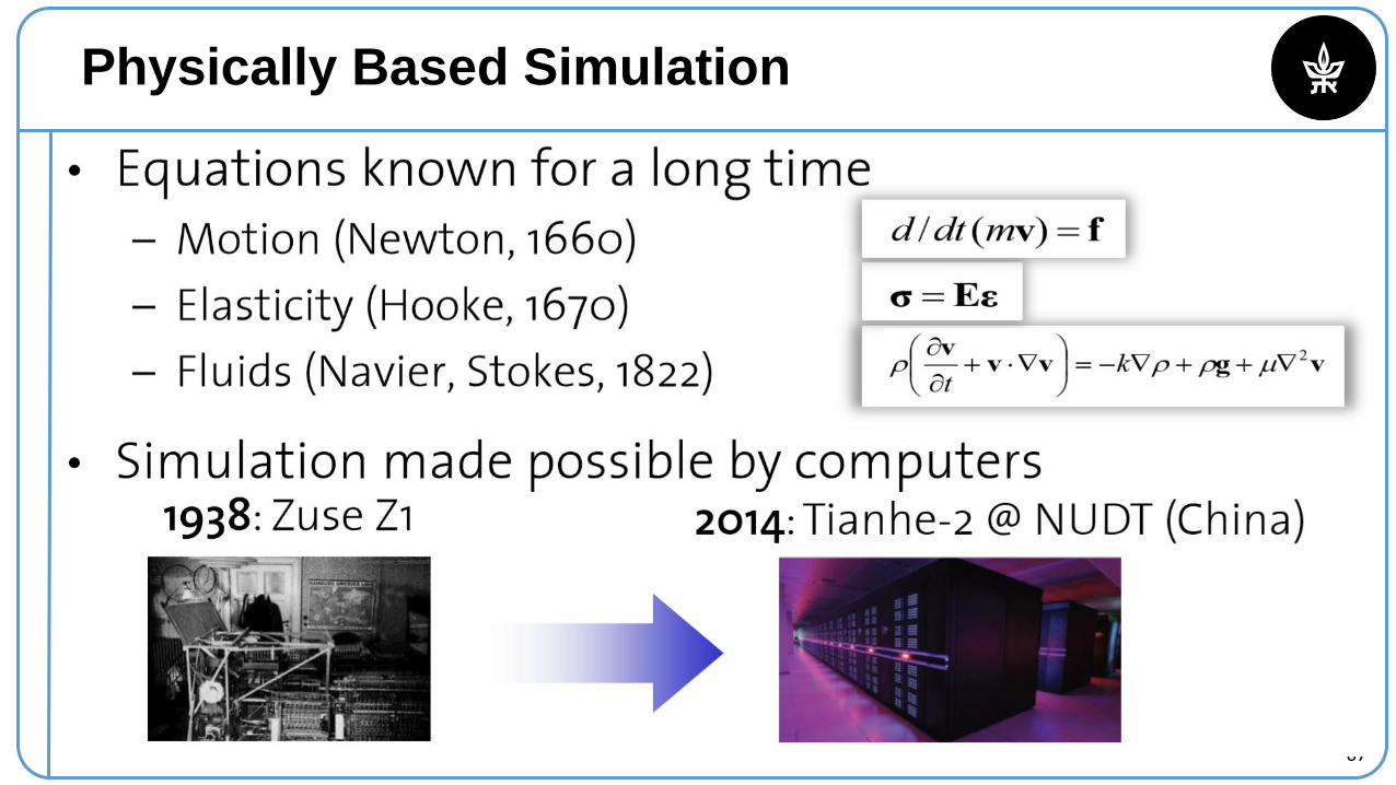
Physically Based Simulation
68
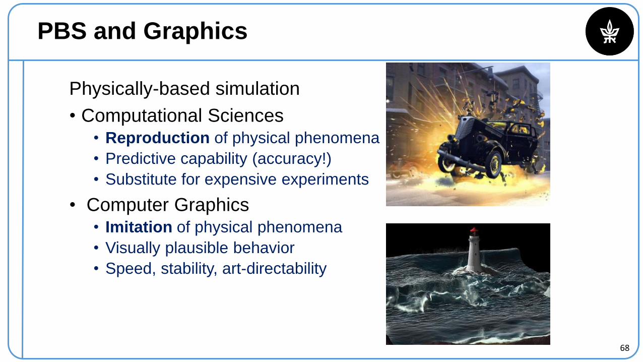
Physically-based simulation
• Computational Sciences• Reproduction of physical phenomena
• Predictive capability (accuracy!)
• Substitute for expensive experiments
• Computer Graphics• Imitation of physical phenomena
• Visually plausible behavior
• Speed, stability, art-directability
PBS and Graphics
69
Simulation in Graphics
• Art-directability
70
Simulation in Graphics
• Speed https://www.youtube.com/watch?v=-x9B_4qBAkk
71
Simulation in Graphics
• Stability
https://www.youtube.com/watch?v=tT81VPk_ukU
72
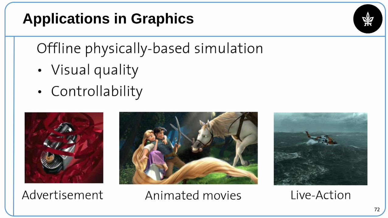
Applications in Graphics
73
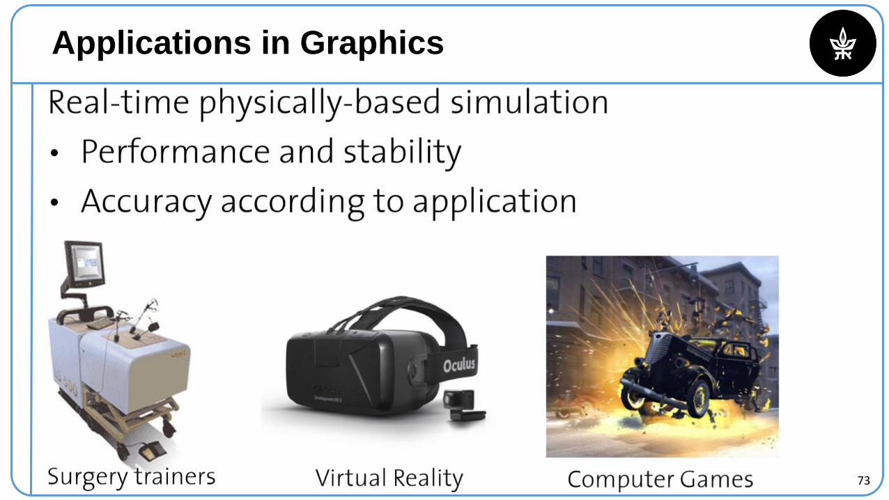
Applications in Graphics
74
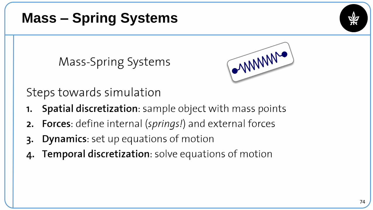
Mass – Spring Systems
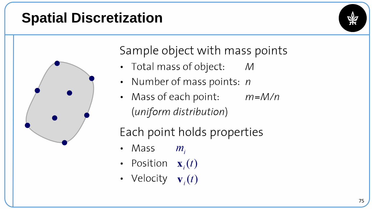
75
Spatial Discretization
76
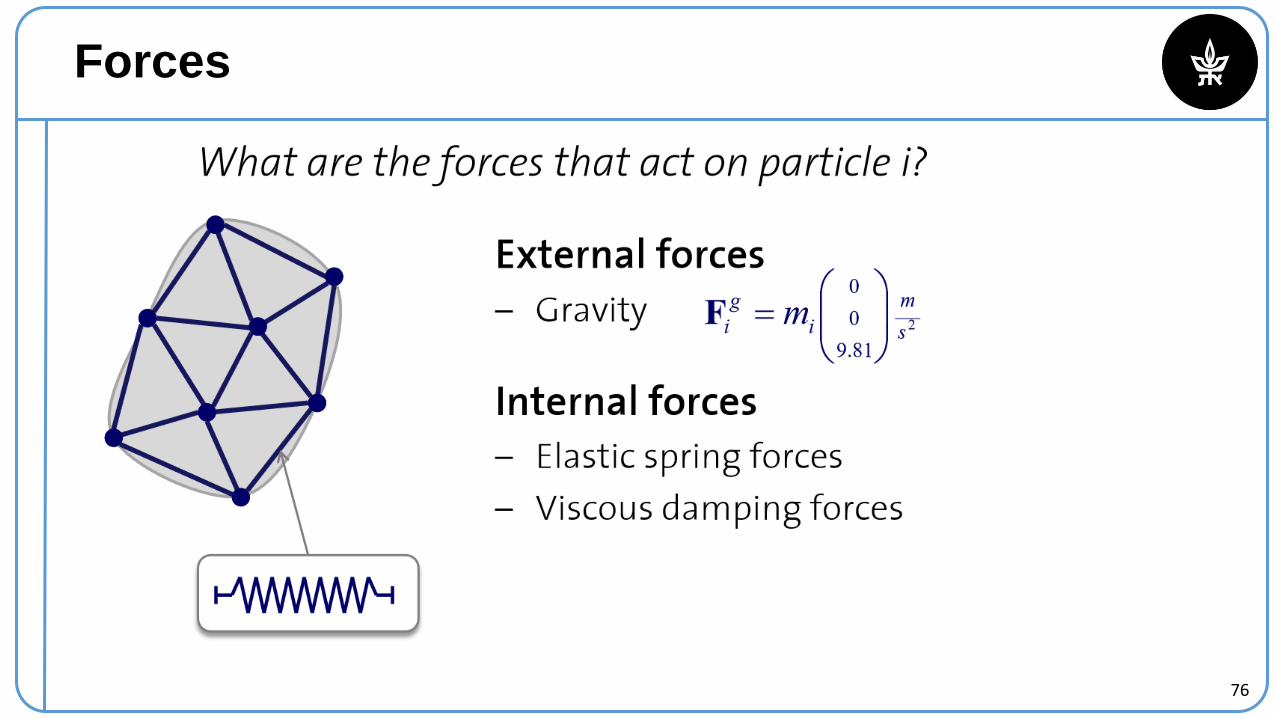
Forces
77
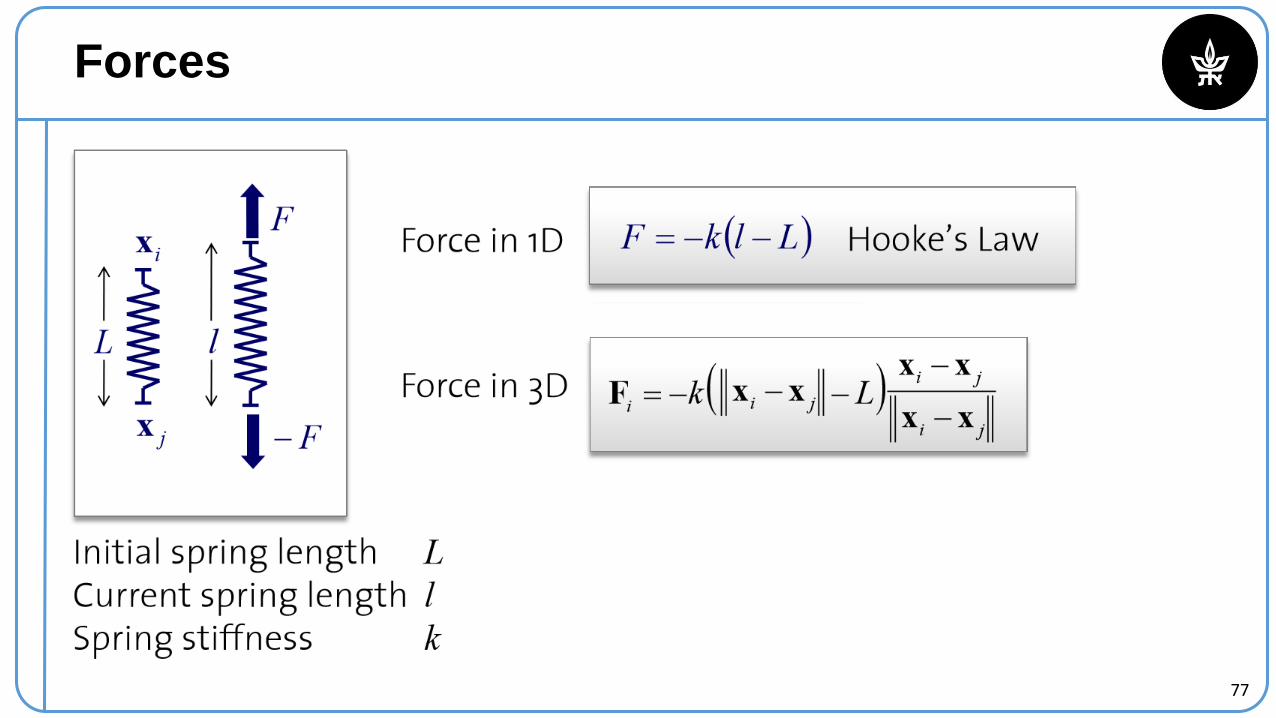
Forces
78
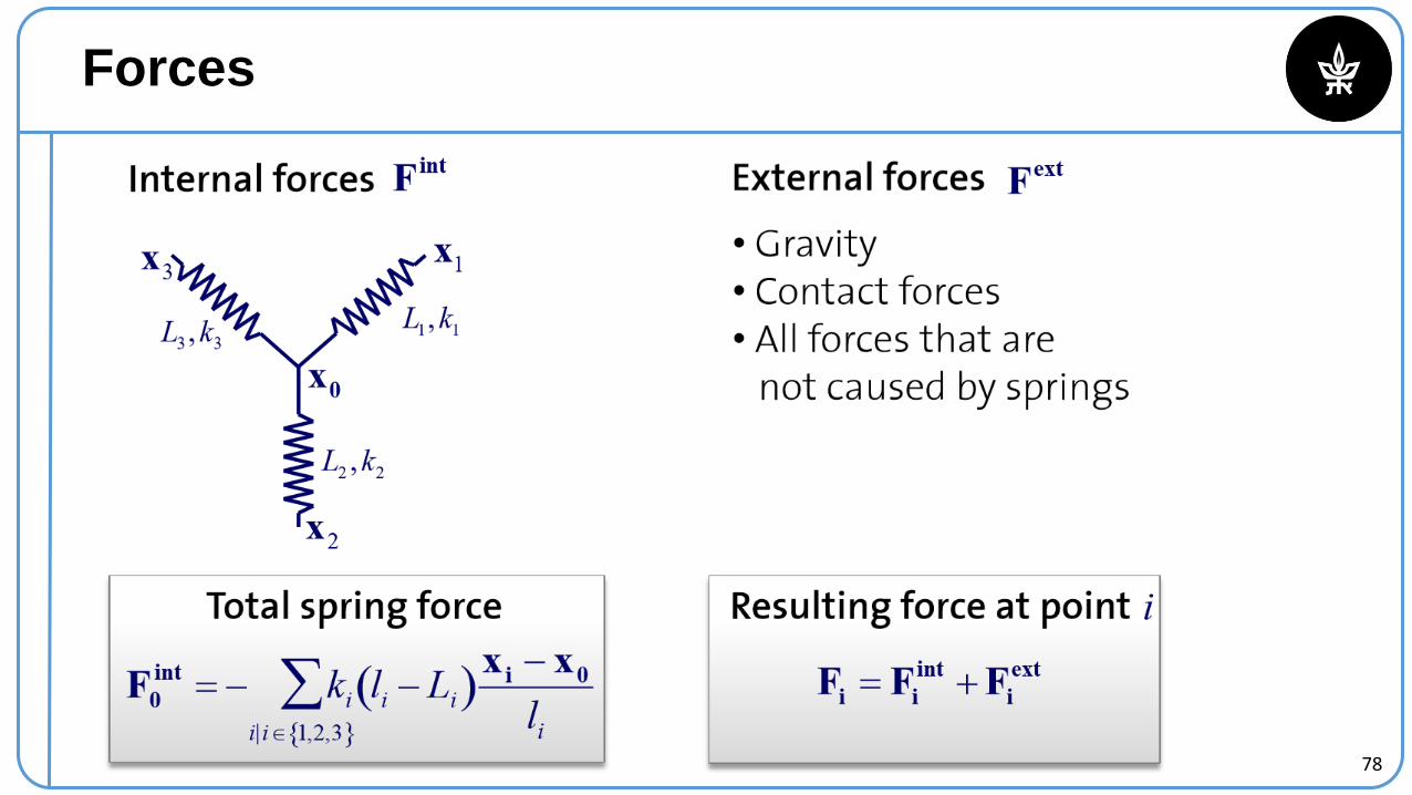
Forces
79
Example: Rope
80
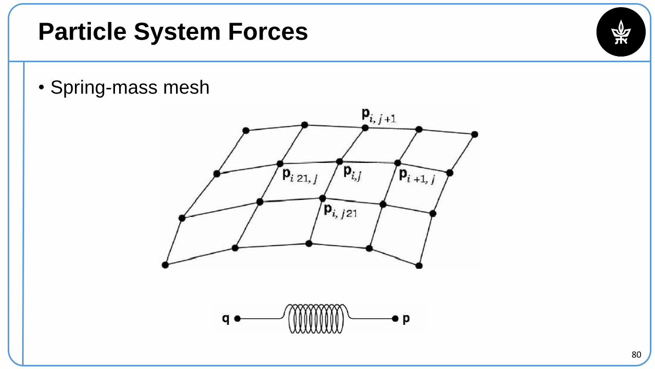
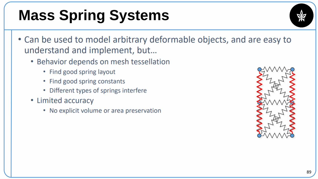
Particle System Forces
• Spring-mass mesh
81
Example: Cloth

82
Demo
83
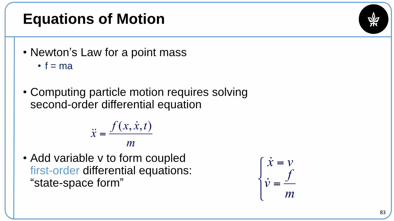
Equations of Motion
• Newton’s Law for a point mass• f = ma
• Computing particle motion requires solvingsecond-order differential equation
• Add variable v to form coupledfirst-order differential equations:“state-space form”
84
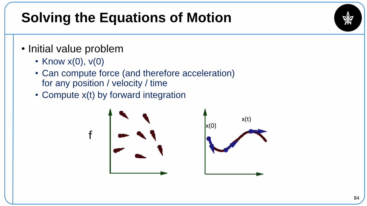
Solving the Equations of Motion
• Initial value problem• Know x(0), v(0)
• Can compute force (and therefore acceleration)for any position / velocity / time
• Compute x(t) by forward integration
fx(0)
x(t)
85
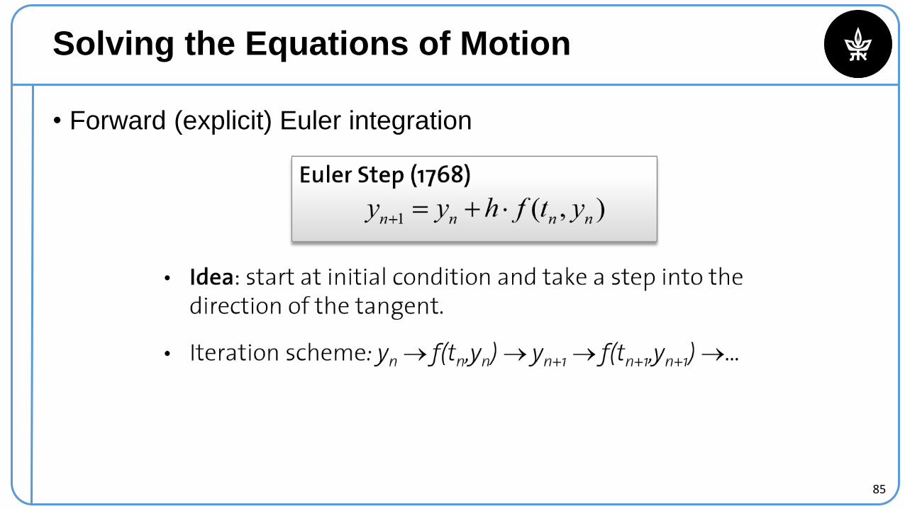
Solving the Equations of Motion
• Forward (explicit) Euler integration
86
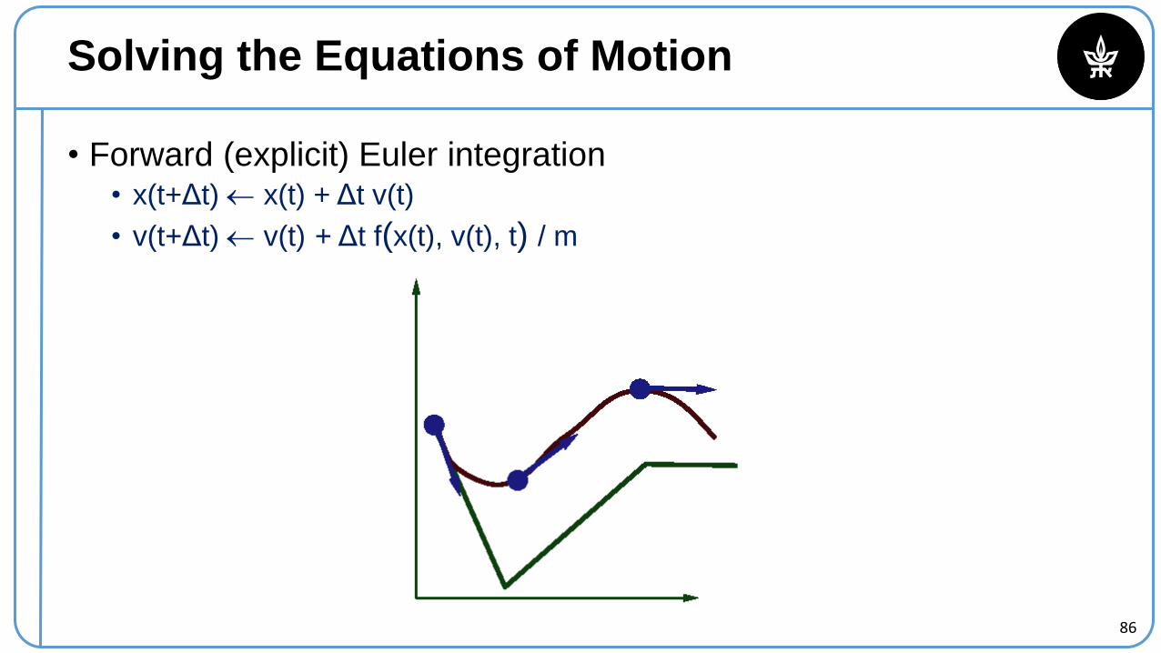
Solving the Equations of Motion
• Forward (explicit) Euler integration• x(t+Δt) x(t) + Δt v(t)
• v(t+Δt) v(t) + Δt f(x(t), v(t), t) / m
87
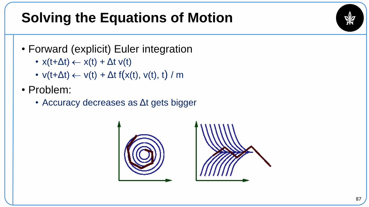
Solving the Equations of Motion
• Forward (explicit) Euler integration• x(t+Δt) x(t) + Δt v(t)
• v(t+Δt) v(t) + Δt f(x(t), v(t), t) / m
• Problem:• Accuracy decreases as Δt gets bigger

88
Single Particle Demo
89
Mass Spring Systems
90
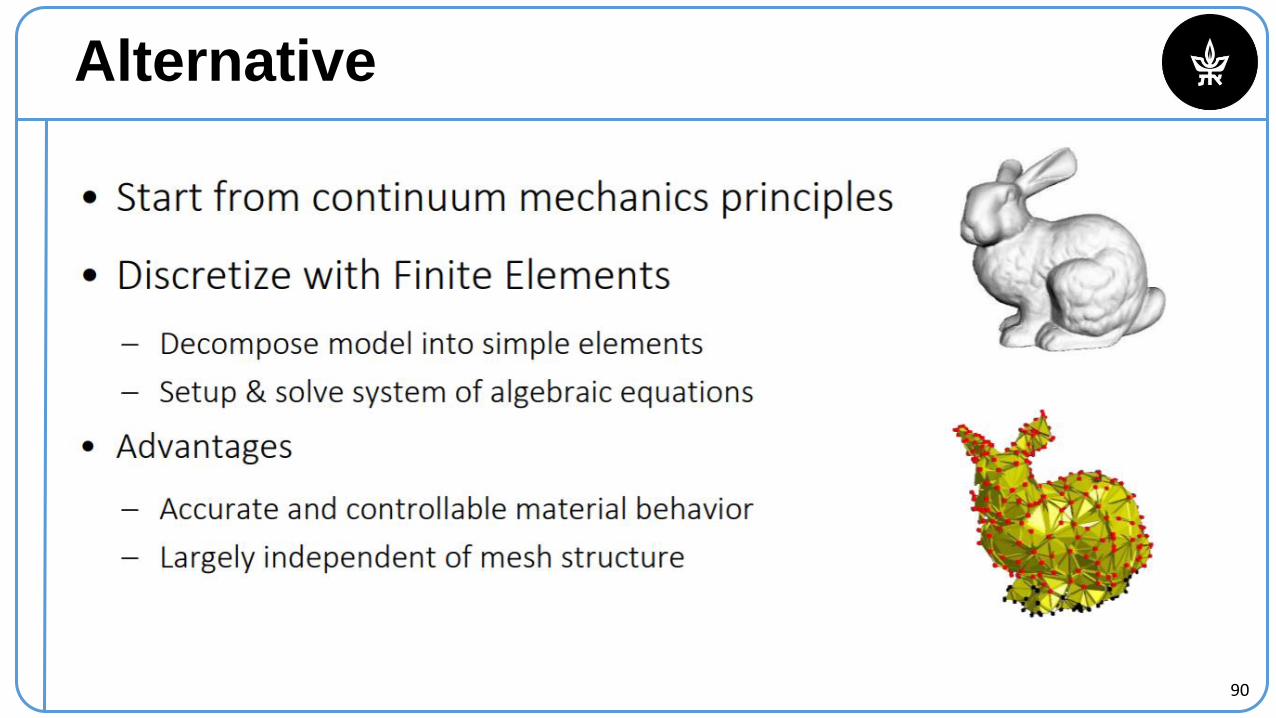
Alternative
91
Continuum Mechanics
https://www.youtube.com/watch?v=BOabEZXm9IE
92
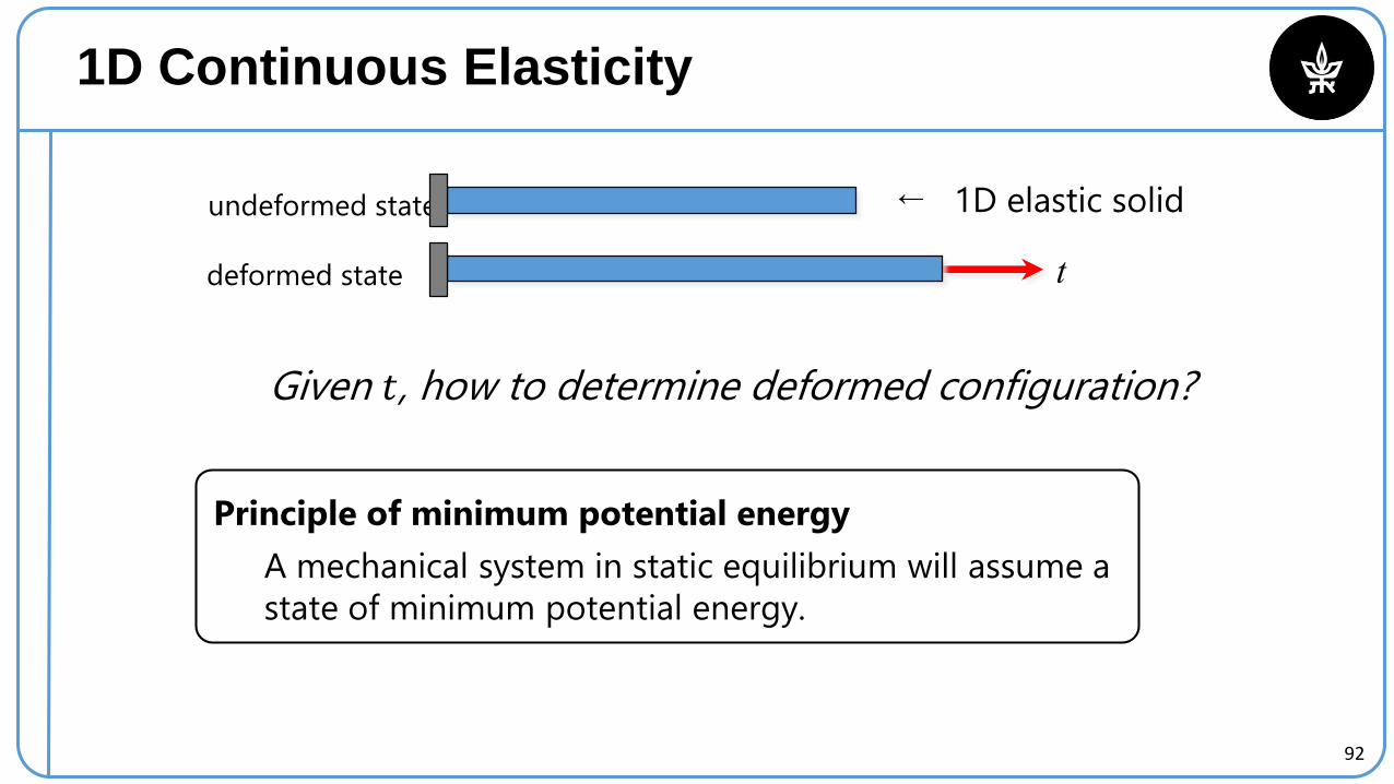
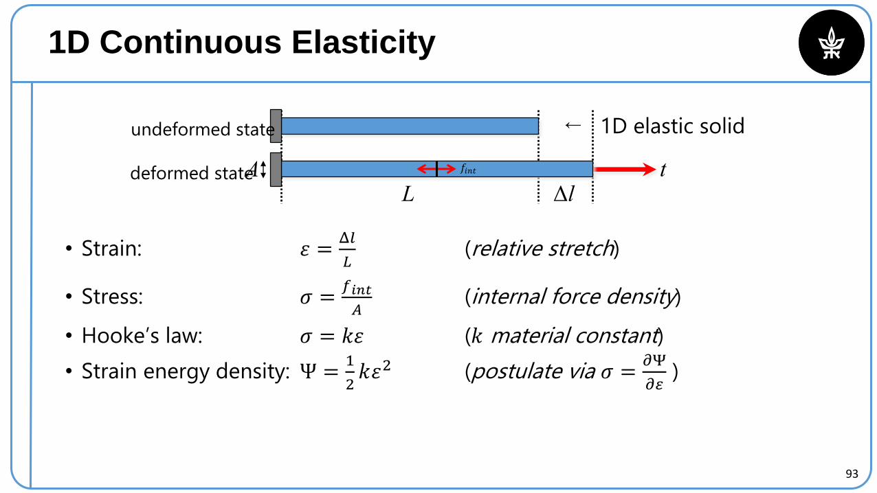
1D Continuous Elasticity
undeformed state 1D elastic solid←
Given 𝑡, how to determine deformed configuration?
Principle of minimum potential energy
A mechanical system in static equilibrium will assume a
state of minimum potential energy.
tdeformed state
93
1D Continuous Elasticity
• Strain: 휀 =Δ𝑙
𝐿(relative stretch)
• Stress: 𝜎 =𝑓𝑖𝑛𝑡
𝐴(internal force density)
• Hooke’s law: 𝜎 = 𝑘휀 (𝑘 material constant)
• Strain energy density: Ψ =1
2𝑘휀2 (postulate via 𝜎 =
𝜕Ψ
𝜕𝜀)
L ΔltA
1D elastic solid←
𝑓𝑖𝑛𝑡
undeformed state
deformed state
94
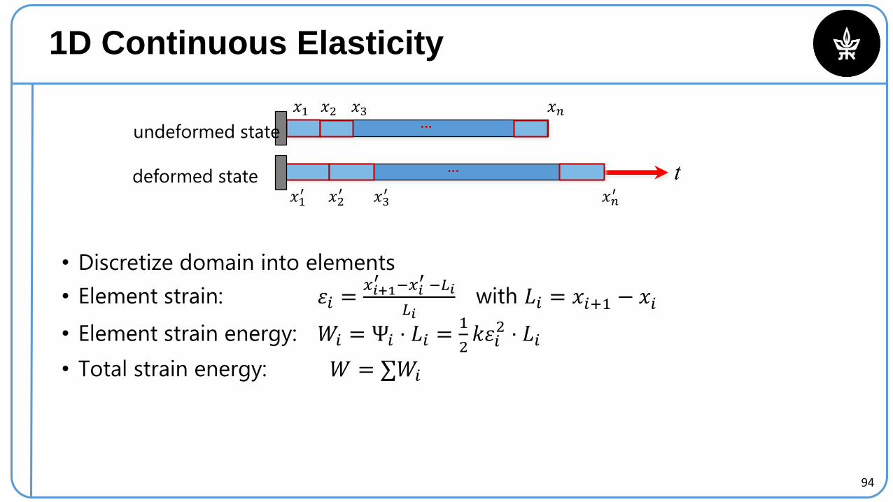
1D Continuous Elasticity
• Discretize domain into elements
• Element strain: 휀𝑖 =𝑥𝑖+1′ −𝑥𝑖
′ −𝐿𝑖
𝐿𝑖with 𝐿𝑖 = 𝑥𝑖+1 − 𝑥𝑖
• Element strain energy: 𝑊𝑖 = Ψ𝑖 ⋅ 𝐿𝑖 =1
2𝑘휀𝑖
2 ⋅ 𝐿𝑖
• Total strain energy: 𝑊 = ∑𝑊𝑖
t
…
…
𝑥1 𝑥2 𝑥3 𝑥𝑛
𝑥1′ 𝑥2
′ 𝑥3′ 𝑥𝑛
′
undeformed state
deformed state
95
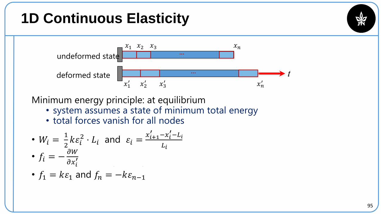
1D Continuous Elasticity
Minimum energy principle: at equilibrium• system assumes a state of minimum total energy • total forces vanish for all nodes
• 𝑊𝑖 =1
2𝑘휀𝑖
2 ⋅ 𝐿𝑖 and 휀𝑖 =𝑥𝑖+1′ −𝑥𝑖
′−𝐿𝑖
𝐿𝑖→
𝜕𝑊𝑖
𝜕𝑥𝑖′ =
𝜕𝑊𝑖
𝜕𝜀𝑖
𝜕𝜀𝑖
𝜕𝑥𝑖′ = −𝑘휀𝑖
• 𝑓𝑖 = −𝜕𝑊
𝜕𝑥𝑖′ = −
𝜕𝑊𝑖−1
𝜕𝑥𝑖′ −
𝜕𝑊𝑖
𝜕𝑥𝑖′ = −𝑘(휀𝑖−1 − 휀𝑖) for 𝑖 = 2…𝑛 − 1
• 𝑓1 = 𝑘휀1 and 𝑓𝑛 = −𝑘휀𝑛−1
t
…
…
𝑥1 𝑥2 𝑥3 𝑥𝑛
𝑥1′ 𝑥2
′ 𝑥3′ 𝑥𝑛
′
undeformed state
deformed state
96
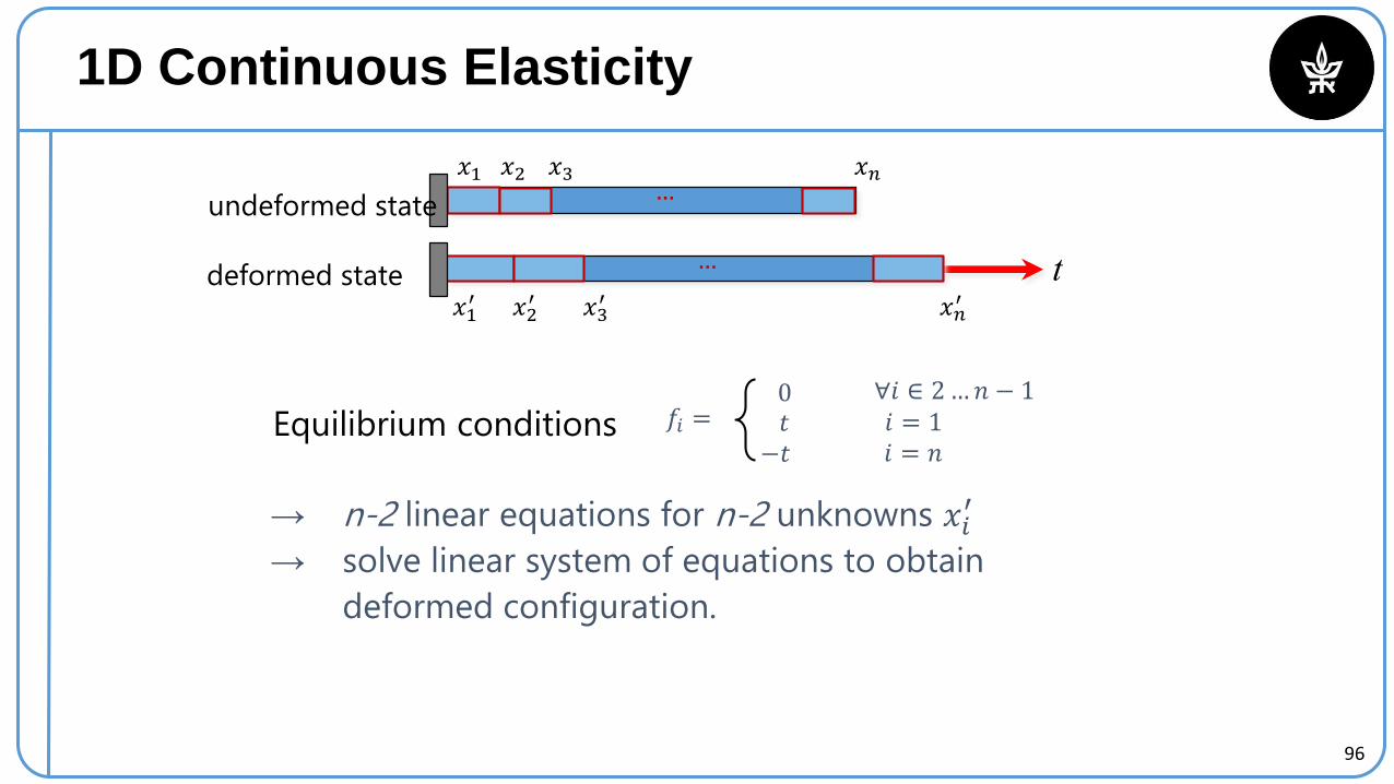
1D Continuous Elasticity
Equilibrium conditions 𝑓𝑖 =0 ∀𝑖 ∈ 2…𝑛 − 1
−𝑡 𝑖 = 𝑛
→ n-2 linear equations for n-2 unknowns 𝑥𝑖′
→ solve linear system of equations to obtain
deformed configuration.
t
𝑥1…
…
𝑥2 𝑥3 𝑥𝑛
𝑥1′ 𝑥2
′ 𝑥3′ 𝑥𝑛
′
𝑡 𝑖 = 1
undeformed state
deformed state
97
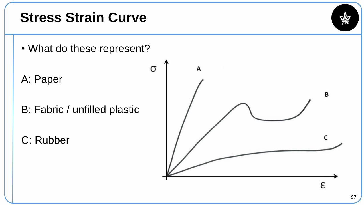
Stress Strain Curve
• What do these represent?
A: Paper
B: Fabric / unfilled plastic
C: Rubber
98
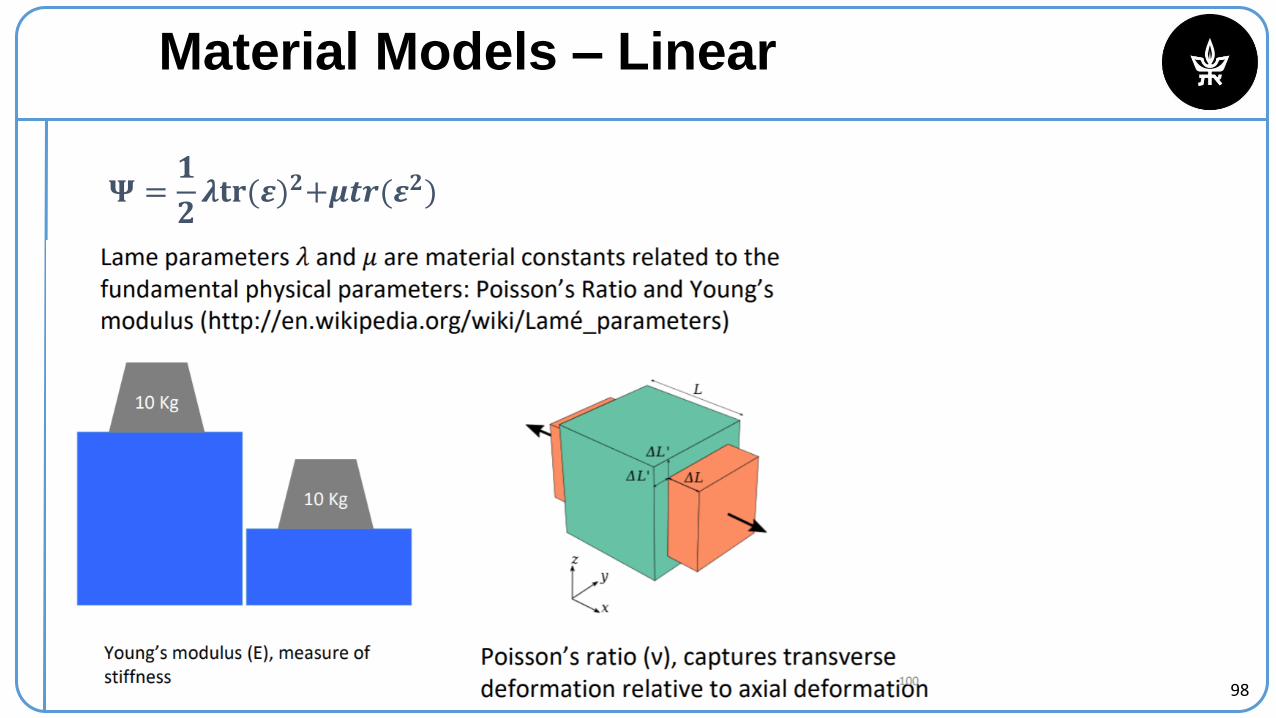
Material Models – Linear
𝚿 =𝟏
𝟐𝝀𝐭𝐫(𝜺)𝟐+𝝁𝒕𝒓(𝜺𝟐)
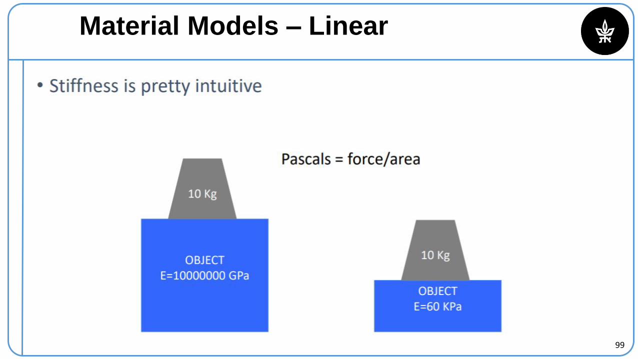
99
Material Models – Linear
100
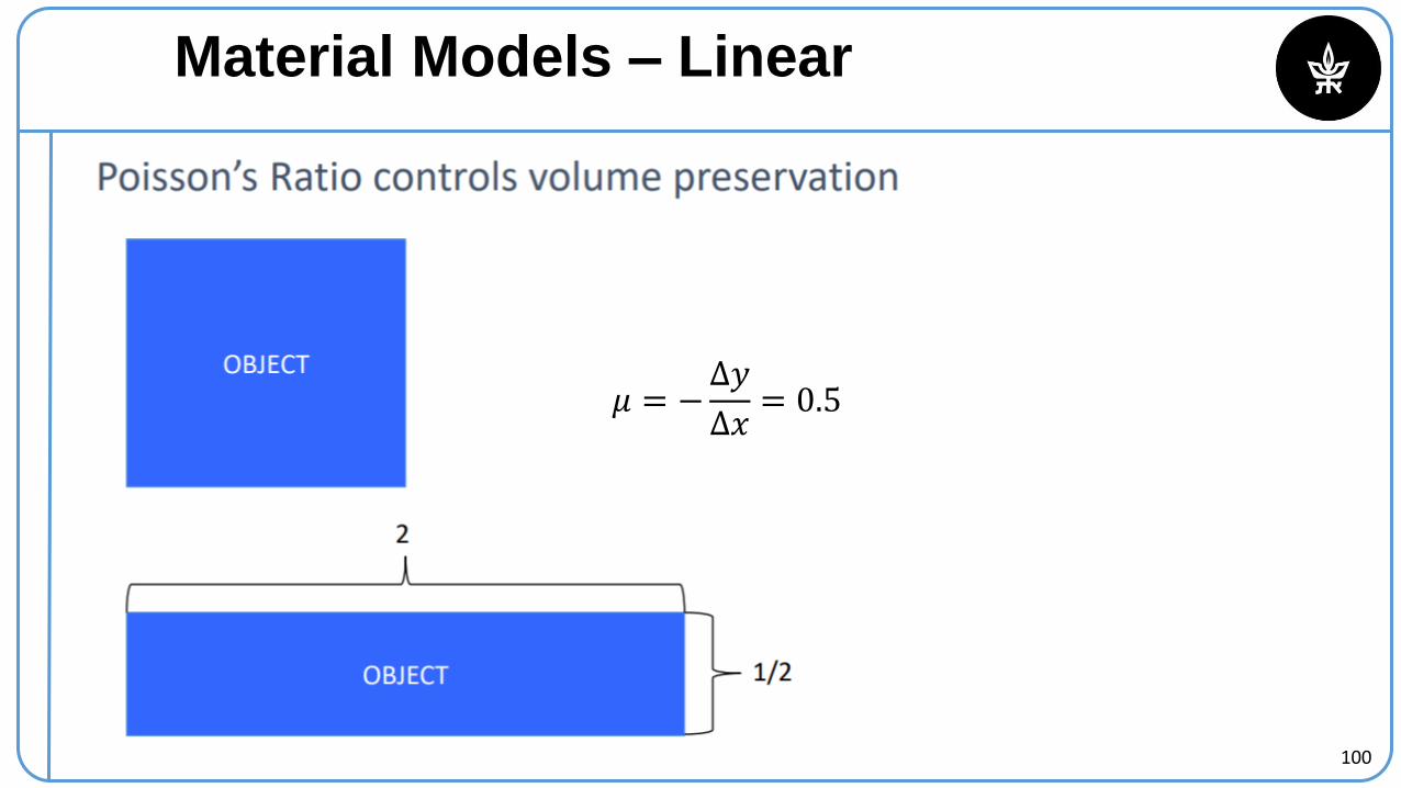
Material Models – Linear
𝜇 = −Δ𝑦
Δ𝑥= 0.5
101
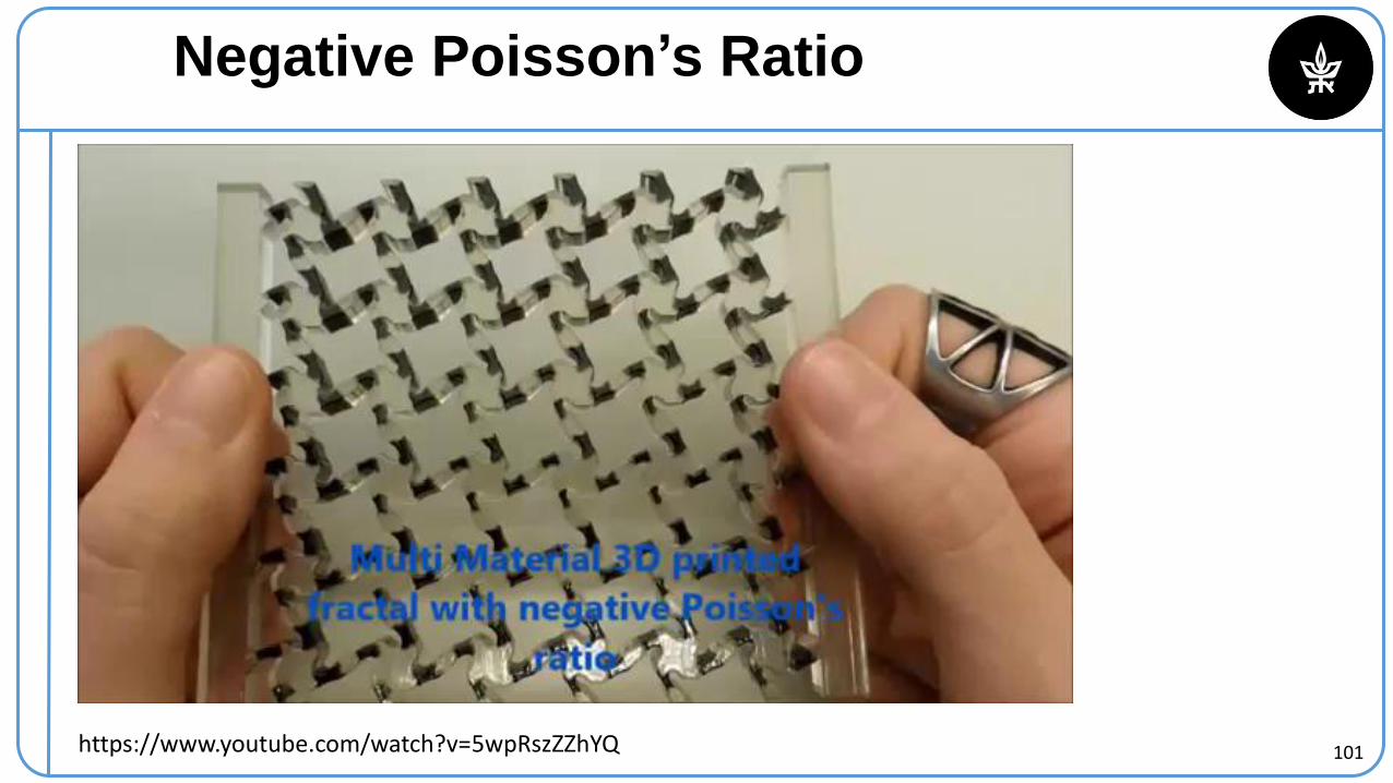
Negative Poisson’s Ratio
https://www.youtube.com/watch?v=5wpRszZZhYQ
103
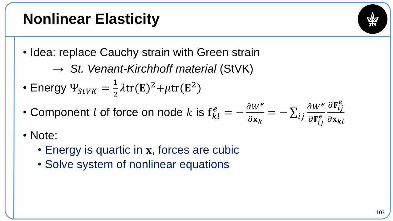
Nonlinear Elasticity
• Idea: replace Cauchy strain with Green strain
→ St. Venant-Kirchhoff material (StVK)
• Energy Ψ𝑆𝑡𝑉𝐾 =1
2𝜆tr(𝐄)2+𝜇tr(𝐄2)
• Component 𝑙 of force on node 𝑘 is 𝐟𝑘𝑙𝑒 = −
𝜕𝑊𝑒
𝜕𝐱𝑘= −∑𝑖𝑗
𝜕𝑊𝑒
𝜕𝐅𝑖𝑗𝑒
𝜕𝐅𝑖𝑗𝑒
𝜕𝐱𝑘𝑙
• Note:
• Energy is quartic in 𝐱, forces are cubic
• Solve system of nonlinear equations
104
Nonlinear Elasticity
105
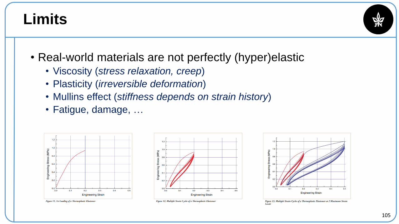
Limits
• Real-world materials are not perfectly (hyper)elastic• Viscosity (stress relaxation, creep)
• Plasticity (irreversible deformation)
• Mullins effect (stiffness depends on strain history)
• Fatigue, damage, …
106
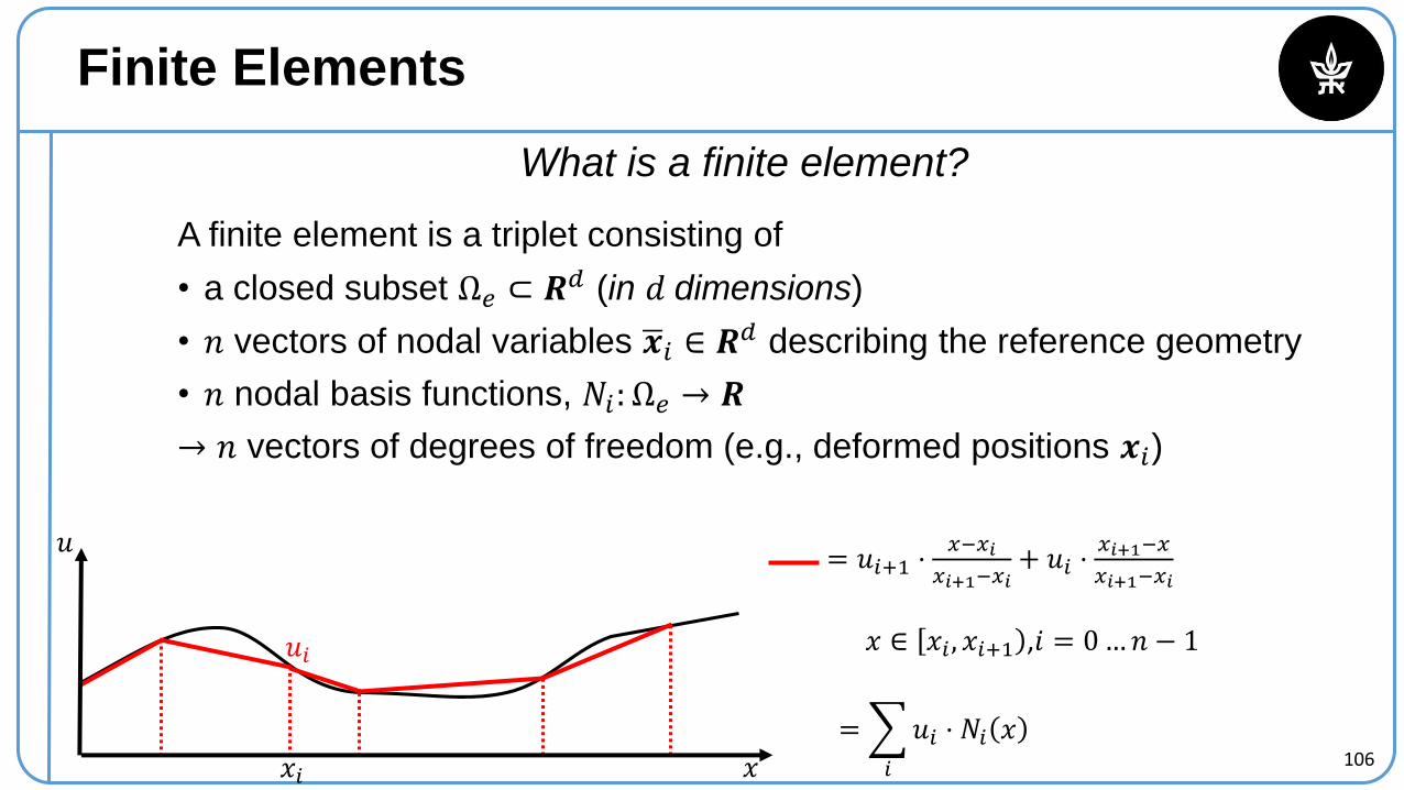
Finite Elements
What is a finite element?
A finite element is a triplet consisting of
• a closed subset Ω𝑒 ⊂ 𝑹𝑑 (in 𝑑 dimensions)
• 𝑛 vectors of nodal variables ഥ𝒙𝑖 ∈ 𝑹𝑑 describing the reference geometry
• 𝑛 nodal basis functions, 𝑁𝑖: Ω𝑒 → 𝑹
→ 𝑛 vectors of degrees of freedom (e.g., deformed positions 𝒙𝑖)
𝑥
𝑢
𝑥𝑖
𝑢𝑖
= 𝑢𝑖+1 ⋅𝑥−𝑥𝑖
𝑥𝑖+1−𝑥𝑖+ 𝑢𝑖 ⋅
𝑥𝑖+1−𝑥
𝑥𝑖+1−𝑥𝑖
𝑥 ∈ 𝑥𝑖 , 𝑥𝑖+1 ,𝑖 = 0…𝑛 − 1
=
𝑖
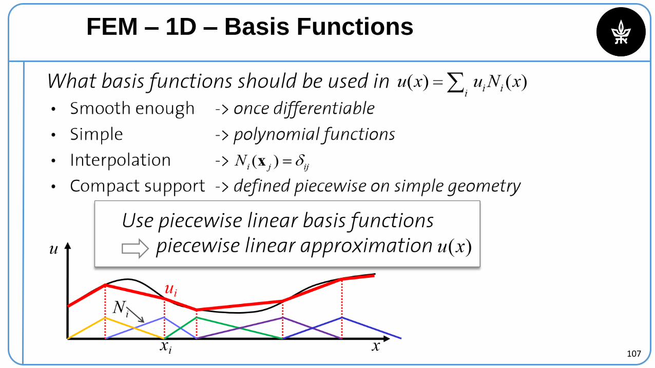
𝑢𝑖 ⋅ 𝑁𝑖 𝑥
107
FEM – 1D – Basis Functions
108
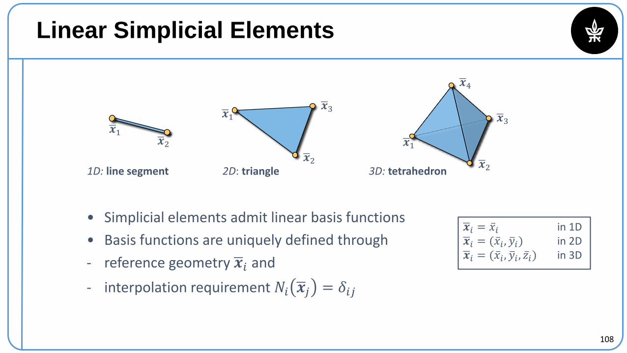
Linear Simplicial Elements
1D: line segment 2D: triangle 3D: tetrahedron
• Simplicial elements admit linear basis functions
• Basis functions are uniquely defined through
- reference geometry ഥ𝒙𝑖 and
- interpolation requirement 𝑁𝑖 ഥ𝒙𝑗 = 𝛿𝑖𝑗
ഥ𝒙𝑖 = ҧ𝑥𝑖 in 1Dഥ𝒙𝑖 = ( ҧ𝑥𝑖 , ത𝑦𝑖) in 2Dഥ𝒙𝑖 = ( ҧ𝑥𝑖 , ത𝑦𝑖 , ҧ𝑧𝑖) in 3D
ഥ𝒙1ഥ𝒙2
ഥ𝒙3ഥ𝒙1
ഥ𝒙2
ഥ𝒙4
ഥ𝒙3
ഥ𝒙1
ഥ𝒙2
109
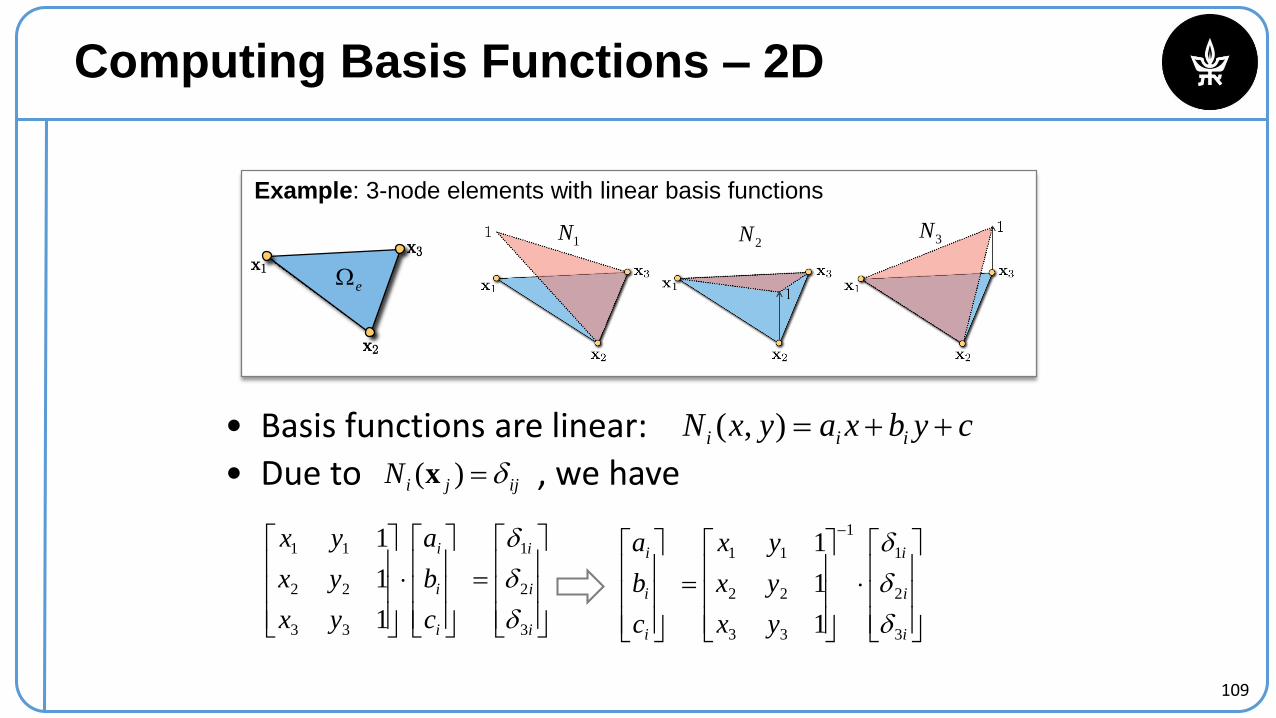
Computing Basis Functions – 2D
i
i
i
i
i
i
c
b
a
yx
yx
yx
3
2
1
33
22
11
1
1
1
i
i
i
i
i
i
yx
yx
yx
c
b
a
3
2
1
1
33
22
11
1
1
1
• Due to , we haveijjiN )(x
Example: 3-node elements with linear basis functions
e
1N2N 3N
• Basis functions are linear: cybxayxN iii ),(
110
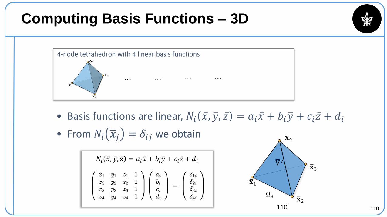
Computing Basis Functions – 3D
110
𝑁𝑖 ҧ𝑥, ത𝑦, ҧ𝑧 = 𝑎𝑖 ҧ𝑥 + 𝑏𝑖 ത𝑦 + 𝑐𝑖 ҧ𝑧 + 𝑑𝑖
Ω𝑒
ത𝐱1
ത𝐱2
ത𝐱3
ത𝐱4
ഥV𝑒
4-node tetrahedron with 4 linear basis functions
… … … …
• Basis functions are linear, 𝑁𝑖 ҧ𝑥, ത𝑦, ҧ𝑧 = 𝑎𝑖 ҧ𝑥 + 𝑏𝑖 ത𝑦 + 𝑐𝑖 ҧ𝑧 + 𝑑𝑖
• From 𝑁𝑖 ഥ𝒙𝑗 = 𝛿𝑖𝑗 we obtain
112
Example
https://www.youtube.com/watch?v=I46ly-ubzYQ
113
Example
https://vimeo.com/245424174