ann aplid to seismic assmnt of deep tunnels
DESCRIPTION
ANN applied to Seismic assmntTRANSCRIPT

Istituto Universitario
di Studi Superiori
Università degli Studi di Pavia
EUROPEAN SCHOOL FOR ADVANCED STUDIES IN REDUCTION OF SEISMIC RISK
ROSE SCHOOL
ARTIFICIAL NEURAL NETWORKS APPLIED TO THE
SEISMIC DESIGN OF DEEP TUNNELS
A Dissertation Submitted in Partial Fulfilment of the Requirements for the Master Degree in
EARTHQUAKE ENGINEERING
by
TERAPHAN ORNTHAMMARATH
Supervisor: Dr CARLO G. LAI, Dr. MIRKO CORIGLIANO
April, 2007

The dissertation entitled “Artificial neural networks applied to seismic design of deep tunnels”, by Teraphan Ornthammarath, has been approved in partial fulfilment of the requirements for the Master Degree in Earthquake Engineering.
Dr. Carlo G. Lai …… … ………
Dr. Mirko Corigliano………… … ……
i

Abstract
ABSTRACT
The underground structure responses in competent rock are widely accepted to conform to the surrounding ground during the earthquake which is different from the aboveground structure responses. Additionally, past study suggested that underground structures in general were less severely affected than surface structures at the same geographic location. However, in the 1995 Kobe, 1999 Chi-Chi, and 1999 Kocaeli earthquakes, the damages of underground structures in these events show that most tunnels were located in the vicinity of the causative fault. One of the main contributions of these damages is the near-fault effect. From the past observations, the near-field ground motions produce ground motion characteristic in the vicinity (<10-25 km) different from that in the far-field because of the directivity and fling step effects. It is important from the practical design point of views to evaluate the seismic performance of underground structures at a particular site, especially in near field. This study presents a simplified method to predict the maximum shear strains around the fault by using Artificial Neural Networks (ANNs). Since the deformation of underground structures, both longitudinal and transversal, is mainly caused by the longitudinal and shear strains respectively in terms of the whole cross section, the proposed method is then based on identification of these shear strains by ANNs. The proposed method is applied to the “Ariano Irpino” fault located in Southern Italy that was subjected to the December 5, 1456 earthquake. The near-field ground motion model developed by Hisada and Bielak [2003] had been performed as this fault with assumed ground profile in that area. The observation point is the point where seismometers or accelerograms would be place to record the ground motion characteristics. The observation points had been assumed to be laid next to the fault in different directions. For this study, it was assumed that we have observation points only in 100- and 600-meter depths. These synthetic data would be used as a training data for ANNs to learn the near-field ground characteristics. From this assumption, the trained ANNs would be able to predict the maximum shear strains in other different directions and depths. The computed results show that the ANNs has a possible capability to predict the maximum shear strains around the fault vicinity. Keywords: deep tunnel; seismic design; artificial neural networks; near-field earthquake
i

Acknowledgement
ACKNOWLEDGEMENTS I would like to express my sincere to a lot of people during my study in MEEES program both in ROSE school, Italy, and UJF, Grenoble: - First of all, I would like to thank Dr. Carlo Lai for introducing to me the topic of seismic design of
tunnels, for his motivation during this work. I also appreciate the financial help provided by the ROSE school during the last stage of this study.
- To Dr. Mirko Corigliano for his guidance, discussion, and reviews of my works, and the good
marks in the homeworks during Prof. Pender’s course. - To all my MEEES and ROSE school students, for all times that we studied, traveled, and got
drunk together. - To my parents, for every phone call that they talked with me when I was home sick. - My final acknowledgement is to my grandmother, who is fighting her last stage of lung cancer,
while I am writing this dissertation. The woman that consoled me when I cried, the woman that held my hand when I was just a little boy, the woman that gave / bought a candy to me when I just came back from school and very hungry, and the woman that asked me about the school after the first day of my primary school. She is always very kind and nice. She always loves and worries about my personal life. I would like to tell her that “Whatever would happen please do not worry I am already a grown up man. I love you as much as you love me. If we had to be separate, I know that you always stay with me and I would be alright because I have you as a mentor to impart invaluable life knowledge; in spite of this, I would miss you the most.”
ii

Index
TABLE OF CONTENTS
Page
ABSTRACT ............................................................................................................................................i ACKNOWLEDGEMENTS....................................................................................................................ii TABLE OF CONTENTS...................................................................................................................... iii LIST OF FIGURES ...............................................................................................................................vi LIST OF TABLES.................................................................................................................................ix 1 INTRODUCTION .............................................................................................................................1
1.1 Objective ....................................................................................................................................4 1.2 General outlines of study ...........................................................................................................5
2 THE DAMAGES TO UNDERGROUND STRUCTURES ..............................................................6 2.1 Typologies of underground structures .......................................................................................6
2.1.1 Support system properties................................................................................................6 2.1.2 Construction Methods......................................................................................................7 2.1.3 Sectional typologies .........................................................................................................7
2.2 The ground motion parameters ..................................................................................................8 2.2.1 Peak Acceleration ............................................................................................................8 2.2.2 Peak Ground Velocity (PGV) ..........................................................................................9 2.2.3 Earthquake magnitude .....................................................................................................9 2.2.4 Duration of earthquake ..................................................................................................10 2.2.5 Frequency-content effects ..............................................................................................10 2.2.6 Near-field ground motion ..............................................................................................11
2.3 The past studies........................................................................................................................14 2.3.1 Dowding and Rozen [1978] ...........................................................................................15 2.3.2 Owen and Scholl [1981] ................................................................................................17 2.3.3 Yoshikawa and Fukuchi [1984] .....................................................................................17
iii

Index
2.3.4 Sharma and Judd [1991] ................................................................................................18 2.3.5 Asakura and Sato [1998]................................................................................................20 2.3.6 American Lifeline Alliance (ALA) [2001] ....................................................................21
2.4 Lesson learns from the past damages.......................................................................................23 2.4.1 Geological settings.........................................................................................................23 2.4.2 Concrete lining...............................................................................................................24 2.4.3 Distance effect ...............................................................................................................24 2.4.4 Overburden depth...........................................................................................................25 2.4.5 Slope stability.................................................................................................................25 2.4.6 Duration of earthquake ..................................................................................................25 2.4.7 Frequency-content effect ...............................................................................................25 2.4.8 Peak ground motion parameters.....................................................................................25 2.4.9 Near-fault effect .............................................................................................................25
3 SEISMIC DESIGN AND ANALYSIS PROCEDURES FOR UNDERGROUND STRUCTURES26 3.1 Seismic behaviors of underground structures ..........................................................................26 3.2 Design and analysis methods ...................................................................................................29
3.2.1 The free field deformation method ................................................................................29 3.2.2 The soil-structure interaction method ............................................................................37 3.2.3 Numerical methods ........................................................................................................49 3.2.4 Conclusion .....................................................................................................................51
4 ARTIFICIAL NEURAL NETWORKS...........................................................................................52 4.1 Introduction to Artificial Neural Networks..............................................................................52
4.1.1 Artificial Neural Networks (ANNs)...............................................................................52 4.1.2 Biological neural networks ............................................................................................52
4.2 Neural Network Architectures .................................................................................................53 4.2.1 Single layer neural network ...........................................................................................54 4.2.2 Multiple layers neural network ......................................................................................54 4.2.3 Other neural network architectures ................................................................................55
4.3 Activation Function .................................................................................................................55 4.3.1 Binary sigmoid function ................................................................................................56 4.3.2 Bipolar sigmoid function ...............................................................................................56
4.4 Training Algorithm ..................................................................................................................56 4.4.1 Learning rule..................................................................................................................56 4.4.2 Generalized delta rule ....................................................................................................57
4.5 The Backpropagation Network ................................................................................................57 4.6 Deficiencies of Backpropagation .............................................................................................61
iv

Index
4.6.1 Network paralysis ..........................................................................................................61 4.6.2 Local minima .................................................................................................................61
5 NUMERICAL EXAMPLES ...........................................................................................................62 5.1 Introduction..............................................................................................................................62 5.2 Test Description and Data Analyzed .......................................................................................62
5.2.1 The case study................................................................................................................62 5.2.2 Near-field ground motion modeling ..............................................................................63 5.2.3 Identification of shear strains by ANNs.........................................................................66
5.3 Results and interpretation of numerical computations.............................................................68 5.3.1 The YZ-shear strain at 0- strike degree axis ..................................................................69 5.3.2 The YZ-shear strain at 270-strike degree axis ...............................................................71 5.3.3 The YZ-shear strain at 280-strike degree axis ...............................................................73 5.3.4 The YZ-shear strain at 315-strike degree axis ...............................................................75 5.3.5 The XY-shear strain at 0-strike degree axis...................................................................77 5.3.6 The XY-shear strain at 270-strike degree axis...............................................................79 5.3.7 The XY-shear strain at 280-strike degree axis...............................................................81 5.3.8 The XY-shear strain at 315-strike degree axis...............................................................83
6 CONCLUSION AND FUTURE RESEARCH ...............................................................................86 6.1 Introduction..............................................................................................................................86 6.2 Numerical examples.................................................................................................................86 6.3 Future research.........................................................................................................................87
REFERENCES .....................................................................................................................................88
v

Index
LIST OF FIGURES
Page
Figure 1.1 Shapes of underground structures [Kawashima, 2000]............................................3
Figure 2.1 An idealization of widely spread underground structure, Kawashima [2000]..........8
Figure 2.2 Different relationships between the pulse period of the velocigram and earthquake
magnitude , Corigliano, M., et al. [2007]..........................................................................11
Figure 2.3 Rupture-directivity effects in the recorded displacement time histories of the 1989
Loma Prieta earthquake, for the fault-normal (top) and fault-parallel (bottom)
components, EERI [1995].................................................................................................12
Figure 2.4 Schematic diagram showing the orientations of fling step and directivity pulse for
...........................................................................................................................................13
Figure 2.5 Schematic diagram of time histories for strike-slip and dip-slip faulting in which 14
Figure 2.6 Calculated peak surface responses with associated damage observations for
earthquakes, Owen and Scholl [1981] ..............................................................................15
Figure 2.7 Comparison of peak ground velocity measured at the free surface and observed
damage, Corigliano, M. [2007].........................................................................................16
Figure 2.8 Damage Statistics, Sharma and Judd [1991] ...........................................................20
Figure 2.9 Seismic forces and probable failure modes, Asakura and Sato [1998]. ..................21
Figure 3.1 Acceleration response of Underground and On-ground structures, [Kawashima,
2000] .................................................................................................................................27
Figure 3.2 Axial deformation along the tunnel, Wang [1993]..................................................28
Figure 3.3 Bending deformation along the tunnel, Wang [1993]. ............................................28
Figure 3.4 Ovaling deformation of a circular cross section [Owen and Scholl, 1981]...........29
Figure 3.5 Geometry of a sinusoidal shear wave oblique to axis of tunnel, Wang [1993].......31
Figure 3.6 Free-field shear distortion of ground Wang [1993].................................................35
vi

Index
Figure 3.7 The interaction between elastic waves and tunnel lining .......................................36
Figure 3.8 Relationship between stress and thickness of tunnel lining, Okamoto[1973].........37
Figure 3.9 Induced forces and moments caused by waves propagating along tunnel axis.......39
Figure 3.10 Induced circumferential forces and moments........................................................44
Figure 3.11 Lining response coefficients vs. flexibility ratio, full-slip interface, and circular
tunnel, Wang [1993] .........................................................................................................45
Figure 3.12 Normalized lining deflection vs. flexibility ratio, full slip interface, and circular
lining, Wang [1993] ..........................................................................................................46
Figure 3.13 Lining (thrust) response coefficient vs. compressibility ratio, no-slip interface,
and circular tunnel, Wang [1993] .....................................................................................48
Figure 3.14 Simplified three-dimensional model for analysis of the global response of an
immersed tube tunnel, Hashash et al. [1998]. ...................................................................50
Figure 4.1 Biological neuron ....................................................................................................53
Figure 4.2 Single layer network................................................................................................54
Figure 4.3 Multiple layer network ............................................................................................55
Figure 4.4 Binary Sigmoid Function ........................................................................................56
Figure 4.5 Bipolar Sigmoid Function .......................................................................................56
Figure 4.6 The diagram illustrates the process of minimizing the error of a function through
the set of empirical data ....................................................................................................58
Figure 4.7 Typical two hidden layers backpropagation neural networks .................................59
Figure 5.1 Location of the “Serro Montefalco” tunnel (dotted line) along the “Caserta-Foggia”
railway line (dark solid line). The nearby active faults retrieved from the DISS 3.0.2
database are superimposed. The “Ariano Irpino” fault (ITGG092), which is assumed as a
potential seismic source in the dynamic analysis of the tunnel, is highlighted. The short
segment perpendicular to the tunnel axis, denotes the cross-section of the tunnel,
Corigliano, M., et al. [2007]. ............................................................................................63
Figure 5.2 Geological profile along the “Serro Montefalco” tunnel, Barla et al. [1986] .........63
Figure 5.3 The crustal velocity profile adopted for the solution of the auxiliary problem,
Corigliano, M., et al. [2007] .............................................................................................64
Figure 5.4 The general outline of the studied fault and its subfaults, Hisada and Bielak [2003]
...........................................................................................................................................66
Figure 5.5 Methodology adopted for this study........................................................................68
Figure 5.6 The general outline of seismic source zone.............................................................69
vii

Index
Figure 5.7 The exact 0-degree YZ-shear strain computed by Hisada code ..............................69
Figure 5.8 The attenuation of PGVs at 0-degree axis ...............................................................70
Figure 5.9 The comparison between 0-degree YZ-shear strain computed by Hisada and ANNs
at different depth ...............................................................................................................70
Figure 5.10 The exact 270-degree YZ-shear strain computed by Hisada code ........................71
Figure 5.11 The attenuation of PGVs at 270-degree axis.........................................................71
Figure 5.12 The comparison between 270-degree YZ-shear strain computed by Hisada and
ANNs at different depths ..................................................................................................72
Figure 5.13 The exact 280-degree YZ-shear strain computed by Hisada code ........................73
Figure 5.14 The attenuation of PGVs at 280-degree axis.........................................................73
Figure 5.15 The comparison between 280-degree YZ-shear strain computed by Hisada and
ANNs at different depths ..................................................................................................74
Figure 5.16 The exact 315-degree YZ-shear strain computed by Hisada code ........................75
Figure 5.17 The attenuation of PGVs at 315-degree axis.........................................................75
Figure 5.18The comparison between 315-degree YZ-shear strain computed by Hisada and
ANNs at different depths ..................................................................................................77
Figure 5.19 The exact 0-degree XY-shear strain computed by Hisada code............................77
Figure 5.20 The attenuation of PGVs at 0-degree axis.............................................................78
Figure 5.21 The comparison between 0-degree XY-shear strain computed by Hisada and
ANNs at different depths ..................................................................................................79
Figure 5.22 The exact 270-degree XY-shear strain computed by Hisada code........................79
Figure 5.23 The attenuation of PGVs at 270-degree axis.........................................................80
Figure 5.24 The comparison between 270-degree XY-shear strain computed by Hisada and
ANNs at different depths ..................................................................................................81
Figure 5.25 The exact 280-degree XY-shear strain computed by Hisada code........................81
Figure 5.26 The attenuation of PGVs at 280-degree axis.........................................................82
Figure 5.27 The comparison between 280-degree XY-shear strain computed by Hisada and
ANNs at different depths ..................................................................................................83
Figure 5.28 The exact 315-degree XY-shear strain computed by Hisada code........................83
Figure 5.29 The attenuation of PGVs at 315-degree axis.........................................................84
Figure 5.30 The comparison between 315-degree XY-shear strain computed by Hisada and
ANNs at different depths ..................................................................................................85
viii

Index
LIST OF TABLES
Page
Table 2.1 Summary of Earthquakes and Lining/Support systems of the Bored tunnels, Power
et al. [1998] .......................................................................................................................22
Table 2.2 Statistics for all bored tunnels, ALA [2001].............................................................22
Table 2.3 Tunnel Fragility-Median PGAs-Ground shaking hazard only, ALA [2001]............23
Table 3.1 Strains and curvatures due to body and surface waves.............................................32
Table 5.1The studied ground profile.........................................................................................65
Table 5.2 The features of studied fault, DISS v. 3.0.2..............................................................65
ix

Chapter 1. Introduction
1 INTRODUCTION
Nowadays, underground tunnel becomes parts of concern to the populace, whether it is for transport or facility purposes. The underground tunnels are still being one of the most challenging problems especially in seismic regions, whose underground structures must sustain both static and seismic phenomena. The seismic responses of tunnels and in general of underground structures is considerably different from that of above-ground facilities since the overall mass of the structure is usually small compared with the mass of the surrounding ground, and the stress confinement provides high values of radiation damping. These two effects make an underground structure to response in accordance with the response of surrounding ground without the resonance. Historically, underground tunnels have experienced a lower rate of damage than aboveground structures; nevertheless, recently several large earthquakes resulted in heavy damage to underground structures in major urban centers and mountain territories. Earthquake effects on underground structures can be grouped into two categories [Hashash et al., 2001]:
1. Ground shaking, i.e. the deformation of the ground produced by seismic waves propagating through the earth's crust.
2. Ground failure such as uplift due to soil liquefaction, fault displacement, and slope instability.
The ground shaking damage, which is the main concern in this report, is caused by the seismic wave propagating through the medium. Some previous studies indicate several reasons for these subsurface facility collapses, which also depend on different earthquake mechanisms, geological settings, and tunnel properties itself [Hashash et al., 2001]. Moreover, different typologies and sizes of underground facilities (e.g. lifelines, repositories, transportation tunnels, etc.) have also been widely acknowledged for their different structural responses from the past damage. It therefore appears prudent to determine under what conditions of anticipated ground shakings, site conditions and opening configurations which are necessary to consider seismic design.
On the other hand, for ground failure damage, which is caused by the fault movement, special design, e.g. a flexible joint, over-sizing the cross section of the tunnel, or reinforcing the shear zone across the fault, needs to be proposed to accommodate the permanent displacement, localized the damage, and provide the means to facilitate repairs. Apart from the direct effect of earthquake ground shaking, the damages from soil liquefaction and slope instability have
1

Chapter 1. Introduction
damaged portals and shallow excavations. The main reasons of these damages are due to the surrounding soil / rock, where the large permanent ground deformation takes place. The ground stabilization techniques, such as soil reinforcement, drainage, grouting, may be effective in preventing damages from liquefiable deposits and slope instability. However, this type of damage is beyond the scope of the present study.
Peak ground motion parameters, such as acceleration and particle velocity, can be correlated with the extent of damage. Duration of the earthquake motion also contributes to damage. Besides earthquake parameters, other important parameters that affect tunnel stability are tunnel support and in-situ stresses. A thorough evaluation of the relation between these parameters, soil conditions, and the performance of the underground structures was not possible because a complete suite of data could not be compiled, since many of the documents citing the earthquake performance of underground structures do not provide details on all the important parameters. Furthermore, many of the events occurred many years ago, and it is no longer possible to obtain complete information on all the relevant factors. Consequently, some empirical relations between various parameters (for example, PGA and PGV), and tunnel damage are approximate and tentative. Then, a more detailed definition of the relationship requires more comprehensive studies than currently available.
In design and analysis of seismic effects, underground structures are classified by Kawashima [2000] into 3 categories (Figure 1.1) based on their structural responses to seismic waves.
1. A pipeline embedded in ground along the surface, most pipelines for utilities are in this group.
2. An underground structure with a large cross section along the ground surface. Underground roads, parking lots, subways and common utility ducts are in this group.
3. An underground structure deep in vertical direction. Large trenches and ducts for ventilation and approaches to tunnels are in this group.
2

Chapter 1. Introduction
Figure 1.1 Shapes of underground structures [Kawashima, 2000]
From past investigations, the underground structures response in accordance to the surrounding soil / rock because of the small mass (inertia) of tunnel compared to the surrounding ground and large radiational damping. Okamoto et al. [1973] measured the seismic response of an immersed tube tunnel during several earthquakes show that the response of a tunnel is dominated by the surrounding ground response not from the inertial properties of the tunnel structure itself. Then, the focus of underground seismic design relies on the estimation of the induced seismic strain and their interaction with the structures. From many underground structural designs, [Wang 1993; Hashash et al. 2001; Corigliano, M., et al. 2007], the accuracy of the stress increment in the tunnel lining evaluated through pseudo-static approach are highly dependent on the prediction of maximum shear strain under the free-field condition. The simplified methods to predict induced seismic strain in the ground should be developed.
However, the general perception of structural and geotechnical engineers was that underground structures presented minimal seismic risk unless they were intersected by active faults, where slip could occur, or liquefaction of the surrounding ground could be triggered. Even current design specifications in USA [AASHTO LRFD, 1998, Interim 2001] for highway structures do not consider the seismic design in the transverse direction unless the structure crosses an active fault. In seismic design for pipeline, the Eurocode 8 suggests the use of simple approaches, Newmark and Kuesel-type of analyses, which are not considered the uncertainty of different geological formations.
The damages of underground structures in the 1995 Kobe, 1999 Chi-Chi, and 2004 Niigata earthquakes, show that most tunnels were located in the vicinity of the causative fault. One of the main contributions of these damages is the near-fault effects, which their ground motions are characterized by strong and coherent (narrow band) long period pulses. The consideration of near-field effects to underground structural design would then be appropriated.
3

Chapter 1. Introduction
However, the near-fault ground motion is also strongly influenced by the fault geometries, which make it even more difficult for the determination of ground motion characteristics in the vicinity area. The direction of rupture propagation relative to the site, termed herein as the rupture-directivity, and possible permanent ground displacements, fling step, are the major effects in near fault region. For vertical strike-slip faults, the rupture directivity effects cause a strong spatial variation in ground motions for a given closest distance to the fault in the direction normal to the fault. In the parallel direction of the vertical strike slip fault, the fling step effect is dominating the ground response. For dip-slip earthquake, however, the effects of rupture directivity and fling step would be concentrated only in the direction normal to the fault.
However, even with considerable knowledge of near-field ground motion, it is just after the 1999 Turkey and 1999 Chi Chi earthquakes that increase the ten-fold of near-field ground motion recordings. For underground structures located in the vicinity of a fault rupture, it is even more difficult to cope with the lacks of near-fault ground motion records and the difficulty to adequately scale the time-histories recorded at the free surface. Synthetic records are then the options for the area in which no properly near-field records. On the other hand, all near-field ground motion records do not include forward rupture directivity effects. This important effect gives even fewer proper data to use in the near-field structural design. This is true even if time histories are being matched to a design spectrum because the spectral matching process cannot build a forward rupture directivity pulse into a record where none is present to begin with, Somerville, P. [2000]. Then, in this study, the semi-analytical near-field ground motion model developed by Hisada and Bielak [2003], which had the capability to generate directivity effect, had been chosen to use through this study. This model is based on the computation of static and dynamic Green’s function of displacements and stresses for a viscoelastic horizontally layered half space.
The application of Artificial Neural Networks (ANNs), which considered as a non-parametric approach, to compute the maximum shear strains in the near-fault ground motion condition would be developed in this study. The ANNs is a powerful and viable tool in satisfactorily emulating complex mapping functions between available and relevant inputs, i.e. acquirable active fault parameters, ground profiles, and outputs, i.e. the maximum shear strains. For the major advantage of ANNs over the physical based-model, considered as a parametric approach, is that an investigated active fault may not behave within the class of models initially assumed. This is also the main reason to hinder the practical engineers and decision-making people to recognize the complex behaviours of near-field ground motion.
1.1 Objective Since the main reason of underground tunnels damages are near fault effect, which its ground motion characteristic in the vicinity (<10-25 km) different from that in the far-field because of the directivity and fling step effects, the consideration of near fault effect in underground structural design is then crucial and inevitable. From many pseudo-static approaches to design underground structures, [Wang 1993; Hashash et al. 2001; Corigliano, M., et al. 2007], it is able to predict the seismic stress increment in the lining if the maximum shear strain is predicted correctly. The application of ANNs to predict the maximum shear strains under free-field condition
4

Chapter 1. Introduction
around the fault would be developed in this study. The main objective of this study can be list below.
1) Assessment of SOA (State Of the Art) on the seismic design of underground structures with a detailed analysis of the typologies of damages caused by earthquakes
2) Development of ANNs for prediction of the maximum shear strains based on the synthetic near-field ground motion generated using Hisada and Bielak [2003] approach.
1.2 General outlines of study The present thesis contains six chapters. It covers the damages to underground structures from earthquakes (Chapter 2), the seismic design and analysis procedures for underground structures (Chapter 3), the general summaries of Artificial Neural Networks (ANNs) (Chapter 4), the numerical examples of the proposed method to predict maximum shear strain using ANNs (Chapter 5). Finally in Chapter 6 the conclusions and future research proposals are presented.
1) The literature of both damaged underground facility and underground seismic design would be reviewed. Also the differences of site characteristics, ground motion parameters, and fault mechanisms, which relate to different structural responses, would then be pointed out. The general summaries about the lesson learn from the past damages would then be provided at the end of the Chapter 2.
2) The seismic behaviors of underground structures would be described at the beginning of the Chapter 3. The current design and analysis of underground structures in the simplified free field deformation and Pseudo-static methods would be reviewed, and investigated their applicability. Some past examples in different approaches would also be provided.
3) The introduction of ANNs would be provided, along with its general procedure, training algorithms, and the deficiencies of ANNs would be provided at the end of Chapter 4.
4) The capabilities of ANNs to reproduce the maximum near-field ground motion shear strains would be performed based on the synthetic near-field ground motion generated by Hisada and Bielak [2003] code. The seismic source would be based on the “Ariano Irpino” fault geometries and characteristics in the “Sannio” region. The data analyzed and the numerical computation procedures would be explained in detailed. The ANNs would be given the sets of training data in order to let the ANNs learning the near-fault characteristics from available data. To generalize and expand its applicability, the input to the ANNs would be available field measurement data which are the soil density, the maximum shear modulus, the PGV, the distance in x and y directions from the fault origin, and the depth of the observation points. At the end of Chapter 5, the trained ANNs would then be able to regenerate the maximum shear strain in the different directions and depths from the trained data.
5
Chapter 2. The Damages to Underground Structures
2 THE DAMAGES TO UNDERGROUND STRUCTURES
The response of underground excavation to earthquake shaking is influenced by many variables. Some important factors of these are the structural typologies and depth of the excavation, the properties of the soil or rock within which the excavation is constructed, the properties of support systems, and the severity of the ground shaking. General concepts of these variables would be provided, and also the past damaged studies to underground structures are described with the explanation about the failure causes. The earthquake characteristics related to damaged of underground structures would be also briefly discussed.
2.1 Typologies of underground structures Since the growing and various use of subsurface facilities in urban area and different ground conditions, their shapes and sizes would then be varied in a wide range resulting in their unique structural responses. Some common types of these structures based on their support systems, construction methods, and sectional typologies, which affect the structural responses in design and analysis, are support system properties, construction methods, and sectional typologies.
2.1.1 Support system properties Underground structural responses within rock and soil can be quite different from each other depending on the strength and quality of the surrounding ground, as well as on the size of the opening. The rock mass can vary from very competent rock with massive blocks to very weak and highly fractured rock. Thus the support requirements can also vary from no support at all to fairly heavy steel sets.
- Lined tunnel, normally, are lined with 0.2 – 0.5 cm of concrete or cast-in-place concrete, where tunnels are excavated in soft rock or where the use of the tunnel requires high safety and infrequent maintenance. The damages of lined tunnel from ground shaking include cracking, spalling, and failure of the liner as a direct consequence of the shaking. Alternatively, vibratory motion may reduce the strength of the ground thereby placing additional loads on the tunnel support system.
- Unlined tunnel will be used where the rock is sound and there is no or little water infiltration. From the past records, however, this type of tunnels is more liable to damage than lined and grouted tunnels even in rock zone, such damage occurs as rock fall, spalling, local opening of rock joints, and block motion.
6

Chapter 2. The Damages to Underground Structures
2.1.2 Construction Methods The linear underground tunnel, which is the main concerned in this study, can be grouped into three broad categorize, each having distinct design features and construction methods. Generally, the reason of different construction methods comes from the different ground conditions.
- Bored or mined tunnel are unique because they are constructed without significantly affecting the soil or rock above the excavation. Tunnels excavated using tunnel-boring machines (TBMs) are usually circular. Situation where boring may be preferable to cut-and-cover excavation include (1) significant excavation depths, and (2) the existence of overlying structures.
- Cut-and-cover structure are those in which an open excavation is made, the structure is constructed, and fill is placed over the finished structure. This method is typically used for tunnels with rectangular cross-section and only for relatively shallow tunnels (< 15 m of overburden). Example of these structures includes subway stations, portal structures. From past experiences, this type of tunnels is more vulnerable than the other methods, since its different soil-structure interaction between backfill and medium. In terms of tunnel performance, the racking behavior of cut-and-cover tunnels appears to be the seismic response most in need of careful attention.
- Immersed tube tunnels are sometimes employed to traverse a body of water. This method involves constructing sections of the structure in a dry dock, then moving these sections, sinking them into position and ballasting or anchoring the tubes in place, Hashash, et al. [2001].
2.1.3 Sectional typologies The shape and size of underground structures can vary in a wide range. They may be classified according to their sizes and shapes into three groups.
- Laterally long (or linear) underground structures, e.g. pipeline utilities, underground tunnel, are more affected to the axial deformation than flexural deformation, while the effect of flexural deformation increases as the size increases, Kawashima [2000].
- Large cross-sectional structures, e.g. underground roads, parking lots, subways, and common utility ducts, are more subjected to in-plane deformation along the cross section. And also because of its shape which is spread extensively in lateral direction as well as longitudinal direction, the beam-type analysis is not realistic. This could be extend to the property of subsurface ground varies in not only longitudinal direction but also transverse direction. Then, an idealization of the structure by plate elements, Figure 2.1, may be more realistic, Kawashima [2000].
7

Chapter 2. The Damages to Underground Structures
Figure 2.1 An idealization of widely spread underground structure, Kawashima [2000]
- Vertically deep underground structures, e.g. large trenches and ducts for ventilation and approaches to tunnels, are more subjected to in-plane deformation along the cross section. In analyzing a vertically deep underground structure, three-dimensional and axi-symmetric finite element idealizations are generally used. However, two-dimensional analysis also provides sufficiently accurate results when a structure is sufficiently stiff compared to the ground, Kawashima [2000].
2.2 The ground motion parameters The ground motion parameters are essential for describing the important characteristics of strong ground motion in compact, quantitative form. Many parameters have been proposed to characterize the amplitude, frequency content, and duration of strong ground motions; some describe only one of these characteristics, while others may reflect two or three. Because of the complexity of earthquake ground motions, identification of a single parameter that accurately describes all important ground motion characteristics is regarded as impossible, [Jenning, 1985; Joyner and Boore, 1988].
2.2.1 Peak Acceleration The most commonly used measure of the amplitude of a particular ground motion is the peak horizontal acceleration (PHA). The PHA for a given component of motion is simply the
8

Chapter 2. The Damages to Underground Structures
largest (absolute) value of horizontal ground acceleration obtained from the accelerogram of that component. By taking the vector sum of two orthogonal components, the maximum resultant Peak Horizontal Acceleration (PHA) (the direction of which will usually not coincide with either of the measured components) can be obtained. For most earthquakes, the horizontal acceleration is greater than the vertical acceleration, and thus the peak horizontal ground acceleration also turns out to be the peak ground acceleration (PGA).
Ground motions with high peak accelerations are usually, but not always, more destructive than motions with lower peak accelerations. Very high peak accelerations that last for only a short period of time may cause little damage to many types of structures. Although peak acceleration is a very useful parameter, it provides no information on the frequency content or duration of the motion; consequently, it must be supplemented by additional information to characterize a ground motion accurately, Kramer [1996].
While a surface structure responds as a resonating cantilevered beam, an underground structure responds essentially with the ground, and then the PGA is not a good parameter to describe the underground responses. The PGA seems to correlate with the extent of damage. However, it is also dependent on the surrounding ground. A severe damage is often associated with tunnels in soil and poor rock; where as damage to tunnels in competent rock is usually (but not always) minor.
2.2.2 Peak Ground Velocity (PGV) The peak ground velocity (PGV) is another useful parameter for characterization of ground motion amplitude. Since the velocity is less sensitive to the high-frequency components of the ground motions, the PGV is more likely than the PGA to characterize ground motion amplitude accurately at intermediate frequencies. Moreover, the PGV is very importance for underground structural design, since a rough estimate of the maximum shear strain could be computed using the following well-known expression, Newmark [1967] relating the peak ground strain (PGS) to the Peak Ground Velocity (PGV):
PGVPGSC
= (2.1)
where C denotes either the apparent speed of propagation velocity of S-waves in the horizontal direction (VSapp) or the prevailing phase velocity of Rayleigh waves (VR).
2.2.3 Earthquake magnitude The earthquake magnitude is a number characteristic of the earthquake depending on the release of energy at the focus and independent of the location of the recording station. Several different magnitudes scales are currently in use, the most common being the local magnitude, ML; the surface wave magnitude, MS; the body wave magnitude, MB; and the moment magnitude, MW. Physically, the magnitude has been correlated with the energy released by the earthquake, as well as the fault rupture length, and maximum displacement, St. John and Zahrah [1987]. A standard magnitude scale that is completely independent of the type of instrument is the moment magnitude, and it comes from the seismic moment M0.
9

Chapter 2. The Damages to Underground Structures
0log 10.71.5w
MM = − (2.2)
where M0 is
0M Adμ= (2.3)
where μ is the shear modulus of the faulted rock (about 3.3×10¹⁰N/m2), A is the area of the fault (i.e. the product of its length and width), and d is the average displacement on the fault (i.e. the slip which is the length of the slip vector of the rupture measured in the plane of the fault).
2.2.4 Duration of earthquake The level of earthquake damage is often strongly influenced by the duration of strong ground motion. For the near-fault effect, the forward directivity time duration is short but with high intensity.
Bommer and Martinez-Pereira [1999] review almost thirty different definitions of strong-motion duration, which have been proposed by various researchers since 1962. They identify three generic groups: bracketed duration, uniform duration and significant duration. They show that the use of different definitions can give rise to very different duration values for any given strong-motion record. Selection of a specific definition should therefore depend on purpose.
2.2.5 Frequency-content effects The earthquake responses of structures and the ground are highly influenced by the frequency content of the input motion. Frequency content is significant for buried structures in as much as the response of the soil layers in which they are embedded is sensitive to frequency content. It is therefore important to consider how the amplitude of ground motion is distributed among the range of frequencies. For the near-fault effect, the frequency content of the forward directivity effect is narrow band and low to intermediate frequency.
For the pulse period of the velocigram several authors proposed empirical correlations between this quantity and moment magnitude (see Figure 2.2). These relations differ mainly for the definitions used for the pulse period and for the database used in the regression analysis.
10

Chapter 2. The Damages to Underground Structures
Figure 2.2 Different relationships between the pulse period of the velocigram and earthquake magnitude ,
Corigliano, M., et al. [2006]
2.2.6 Near-field ground motion In the immediate vicinity of a fault, ground motion exhibits various characteristics that can be attributed to the orientation, direction and other features of propagation of the fault rupture. These factors result in effects termed as “rupture directivity” and “fling step” effects. These effects are significantly difference from those further away from the seismic source. The estimation of ground motions close to an active fault should account for these characteristics of near-field ground motions.
- Rupture directivity effect
The propagation of fault rupture toward a site at a velocity that is almost as large as the shear wave velocity causes most of the seismic energy from the rupture to arrive coherently in a single large long period pulse of motion which occurs at the beginning of the record. This pulse of motion represents the cumulative effect of most of the seismic radiation from the fault. The radiation pattern of the shear dislocation on the fault causes this large pulse of motion to be oriented in the direction perpendicular to the fault, causing the strike-normal peak velocity to be larger than the strike-parallel peak velocity. The enormous destructive potential of near-fault ground motions was manifested in the 1994 Northridge and 1995 Kobe earthquakes. In each of these earthquakes, peak ground velocities as high as 175 cm/s were recorded, and the period of the near-fault pulse lie in the range of 1 to 2 seconds, comparable to the natural periods of structures such as bridges and mid-rise buildings, many of which were severely damaged, Somerville [2000].
Forward rupture directivity effects occur when two conditions are met: the rupture front propagates toward the site, and the direction of slip on the fault is aligned with the site. The conditions for generating forward rupture directivity effects are readily met in strike-slip faulting, where the rupture propagates horizontally along strike either unilaterally or bilaterally, and the fault slip direction is oriented horizontally in the direction along the strike of the fault. The pulse of motion is typically characterized by large amplitude at intermediate to long periods and short duration. However, not all near-fault locations experience forward
11
Chapter 2. The Damages to Underground Structures
rupture directivity effects in a given event. Backward directivity effects, which occur when the rupture propagates away from the site, give rise to the opposite effect: long duration motions having low amplitudes at long periods, Somerville [2000]. Neutral directivity occurs for sites located off to the side of the fault rupture surface (i.e., rupture is neither predominantly toward nor away from the site).
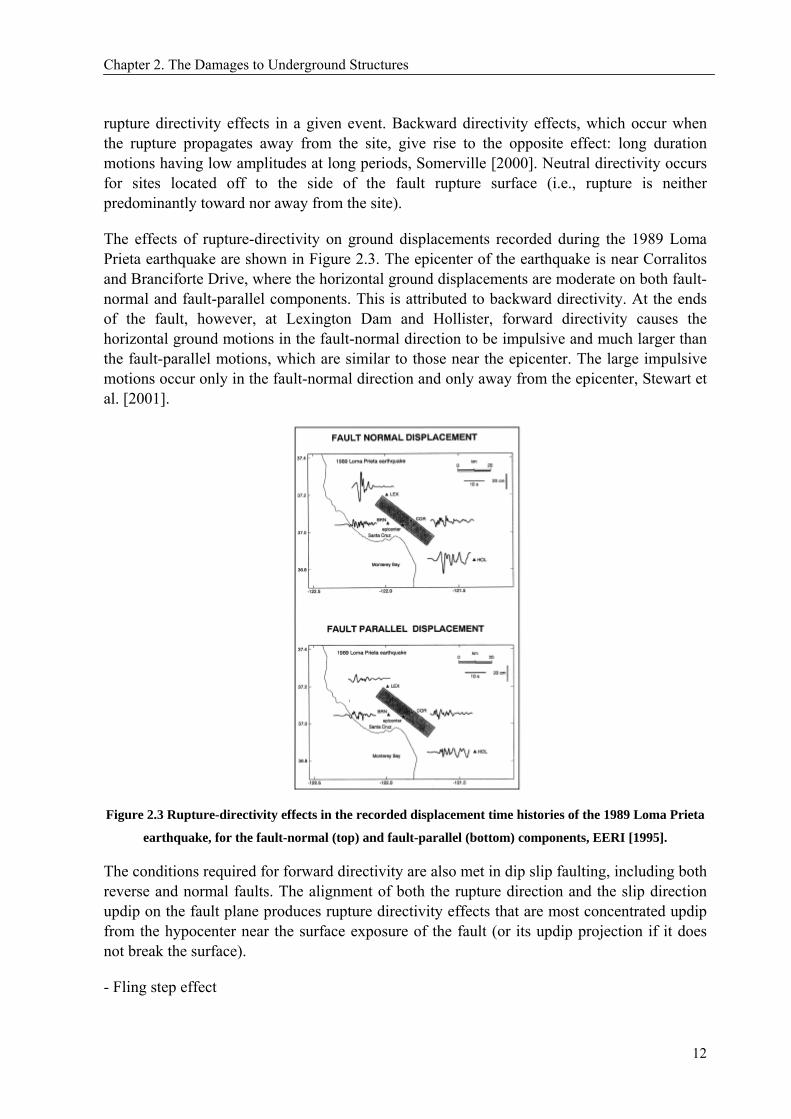
The effects of rupture-directivity on ground displacements recorded during the 1989 Loma Prieta earthquake are shown in Figure 2.3. The epicenter of the earthquake is near Corralitos and Branciforte Drive, where the horizontal ground displacements are moderate on both fault-normal and fault-parallel components. This is attributed to backward directivity. At the ends of the fault, however, at Lexington Dam and Hollister, forward directivity causes the horizontal ground motions in the fault-normal direction to be impulsive and much larger than the fault-parallel motions, which are similar to those near the epicenter. The large impulsive motions occur only in the fault-normal direction and only away from the epicenter, Stewart et al. [2001].
Figure 2.3 Rupture-directivity effects in the recorded displacement time histories of the 1989 Loma Prieta
earthquake, for the fault-normal (top) and fault-parallel (bottom) components, EERI [1995].
The conditions required for forward directivity are also met in dip slip faulting, including both reverse and normal faults. The alignment of both the rupture direction and the slip direction updip on the fault plane produces rupture directivity effects that are most concentrated updip from the hypocenter near the surface exposure of the fault (or its updip projection if it does not break the surface).
- Fling step effect
12

Chapter 2. The Damages to Underground Structures
Moreover, the effects of surface faulting due to tectonic deformations have been recently called fling step. These static displacements occur over a discrete time interval of several seconds as the fault slip is developed. In contrast to forward directivity effects, which show the large long-period pulse in the direction normal to the fault plane, the fling effects exhibit long-period pulses and permanent static offsets in the direction parallel to the fault plane, and therefore are not strongly coupled with the aforementioned dynamic displacements referred to as the “rupture-directivity pulse”. In dip-slip faulting, both the fling step and directivity pulse occur on the strike-normal component. The orientations of fling step and directivity pulse for strike-slip and dip-slip faulting are shown schematically in Figure 2.4, and time histories in which these contributions are shown together and separately are shown schematically in Figure 2.5, Stewart et al. [2001].
Figure 2.4 Schematic diagram showing the orientations of fling step and directivity pulse for
strike-slip and dip-slip faulting, Stewart et al. [2001].
13

Chapter 2. The Damages to Underground Structures
Figure 2.5 Schematic diagram of time histories for strike-slip and dip-slip faulting in which
the fling step and directivity pulse are shown together and separately, Stewart et al. [2001].
2.3 The past studies Historically, underground facilities have experienced a lower rate of damage than aboveground structures. However several large earthquakes resulted in damage to modern underground structures both in mountain and urban areas.
Some investigators of the performance of underground excavations have attempted to develop direct empirical relationships between damage levels and ground motion parameters. Such attempts are fraught with difficulties since damage assessments may be highly subjective and the peak ground motion experienced at a site must often be deduced from very incomplete data. Therefore, it is desirable that arrays of strong instruments be deployed in and around important underground structures.
Wang, et al. [2001] reported the various degrees of mountain tunnel damages after the 1999 Chi Chi earthquake. The most and often serious damage were found on the east of the Chelungpu fault line (hanging wall) while damages on the footwall and other areas suffered less. Then, the extent of damage to tunnel linings was influenced by the position of the tunnels in relation to fault zones, ground conditions, and closeness to the epicenter and surface slopes.
14

Chapter 2. The Damages to Underground Structures
Information on the performance of underground openings during earthquakes is relatively scarce, compared to information on the performance of surface structures. Therefore, the summaries of published data presented in this section may represent only a small fraction of the total amount of data on underground structures. There may be many damage cases that went unnoticed or unreported. However, there are undoubtedly even more unreported cases where little or no damage occurred during earthquakes, Indrawan [2001].
2.3.1 Dowding and Rozen [1978] Dowding and Rozen [1978] identified three levels of damage for underground excavations in rock due to ground shaking: these were no damage, minor damage, and damage. No damage meant no new cracks or falls of rocks; minor damage meant new cracking and minor rock falls; and damage included severe cracking, major rock falls, and closure. Dowding and Rozen [1978] presented results of correlation of the estimated peak surface acceleration and peak particle velocity with reported damage. Their correlations are reproduced in Figure 2.6. The numbers on the ordinate axis are the designations of the cases tabulated in their paper. The same numbering system also is used within the extensive tabulation of damage prepared by Owen and Scholl [1981]. It should be noted that the peak ground motion parameters (acceleration and velocity) were not recorded at the sites of the excavations but were calculated using attenuation relationships. Free-field strong motion measurements from instruments placed in and around tunnels could provide much more reliable data in the future.
(a) (b)
(a) peak surface acceleration (b) peak particle velocities
Figure 2.6 Calculated peak surface responses with associated damage observations for earthquakes, Owen
and Scholl [1981]
Review of data such as those presented by Dowding and Rozen [1978] suggests that no
15

Chapter 2. The Damages to Underground Structures
damage should be expected if the peak surface accelerations are less than about 0.2g, and only minor damage should be experienced between 0.2 and 0.4 g. The corresponding thresholds for peak particle velocity are approximately 20 cm/s and 40 cm/s. Of these two correlations, the one based on velocity is probably to be preferred as a design criterion because the peak particle velocity resulting from an earthquake of a given magnitude can be predicted to fall within reasonably narrow limits. Moreover, experience on the performance of mining excavations adjacent to rock bursts has indicated that damage is better correlated with peak velocity than peak acceleration McGarr [1983].
It should be emphasized that the above relationships hold for rock sites only, and may be very different for underground structures in soil because the attenuation of motion with depth and the confinement of the structure are very different than those for rock sites. Unfortunately, similar relationships have not yet been derived for underground structures in soil, St. John and Zahrah [1987].
Dowding and Rozen [1978] also summarized two relationships involving tunnel damage. First, the observed damage is compared to Modified-Mercalli (MM) Intensity levels for aboveground structures. Secondly, the damage level is correlated to Richter magnitude and distance between epicenter and tunnel location. The ‘no damage zone’ with acceleration up to 0.19g, is equivalent to MM VI-VIII; the ‘minor damage zone’ with acceleration up to 0.5g is equivalent to MM VIII – IX. It is clear that at peak surface accelerations which are expected to cause heavy damage to aboveground structures (MM VIII - IX) there is only minor damage to tunnels. Comparatively, then, tunnels are less vulnerable to damage from shaking than aboveground structures at the same intensity level as determined from surface motions. However, the values of PGV suggested by Dowding and Rozen [1978] are typical for near-fault earthquake and for such events the predictions of PGV made by attenuation relations carry a certain level of uncertainty. Bray and Rodriguez-Marek [2004] developed a more reliable relation of PGV in the near fault region. This relation has been used to correlate the PGV to the damage thresholds defined by Dowding and Rozen [1978] as illustrated in Figure 2.7, Corigliano, M. [2007].
Figure 2.7 Comparison of peak ground velocity measured at the free surface and observed damage,
Corigliano, M. [2006].
16

Chapter 2. The Damages to Underground Structures
However, damage resulting from fault displacement must still be considered. Based on their study, Dowding and Rozen [1978], concluded primarily for rock tunnels, that;
- Tunnels are much safer than aboveground structures for a given intensity of shaking.
- Tunnels deep in rock are safer than shallow tunnels
- No damage was found in both lined and unlined tunnels at surface acceleration up to 0.19g
- Minor damage consisting of cracking of brick or concrete or falling of loose stones was observed in a few cases for surface accelerations above 0.25g and below 0.4g.
- No collapse was observed due to ground shaking effect alone up to a surface acceleration of 0.5g
- Severe but localized damage including total collapse may be expected when a tunnel is subject to an abrupt displacement of an intersecting fault.
2.3.2 Owen and Scholl [1981] These authors documented additional case histories to Dowding and Rozen [1978]’s, for a total of 127 case histories. In addition, they suggested the following:
- Little damage occurred in rock tunnels for peak ground accelerations below 0.4g.
- Severe damage and collapse of tunnels from shaking occurred only under extreme conditions, usually associated with marginal construction such as brick or plain concrete liners and lack of grout between wood lagging and the overbreak.
- Severe damage was inevitable when the underground structure was intersected by a fault that slipped during an earthquake. Cases of tunnel closure appeared to be associated with movement of an intersecting fault, landslide, or liquefied soil.
- Deep tunnels were less prone to damage than shallow tunnels.
- Duration of strong seismic motion appeared to be an important factor contributing to the severity of damage to underground structures. Damage initially inflicted by earth movements, such as faulting and landslides, may be greatly increased by continued reversal of stresses on already damaged sections.
2.3.3 Yoshikawa and Fukuchi [1984] These authors described the damage of railway tunnels in Japan from different earthquakes, which magnitude ranging from 7.0 to 7.9. This paper reported a vague tendency of the number of damages not dependent only on the earthquake magnitude, but also on the geological settings of railway tunnels.
The ground failure, which is caused by slope stability, is the main reason of damages from these records, since Japan mountain tunnels have been and are constructed around the sloping
17

Chapter 2. The Damages to Underground Structures
area. The heavy damage could be observed at the intersection of the railway and fault lines. The number of damaged tunnels decreased with respect to the farther distance from the hypocentral zone coinciding with the acceleration attenuation. The high seismic vulnerability of joint portion (e.g. portal part) had also been notified by the authors according to the statistic records. Deformations were mostly tied to faults or where the strata show sudden change in strength.
2.3.4 Sharma and Judd [1991] The authors extended Owen and Scholl [1981]’s work and collected qualitative data for 192 reported observations from 85 worldwide earthquake events. They correlated the vulnerability of underground facilities with six factors: overburden cover, rock type (including soil), peak ground acceleration, earthquake magnitude, epicentral distance, and type of support. It must be pointed out that most of the data reported are for earthquakes of magnitude equal to 7 or greater. Therefore, the damage percentage of the reported data may appear to be astonishingly higher than one can normally conceive.
The results are summarized in the following paragraphs. These statistical data are of a very qualitative nature. In many cases, the damage statistics, when correlated with a certain parameter, may show a trend that violates an engineer’s intuition. This may be attributable to the statistical dependency on other parameters which may be more influential.
- The effects of overburden depths on damage are shown in Fiugre 2.8A for 132 of 192 cases. Apparently, the reported damage decreases with increasing overburden depth.
- Figure 2.8B shows the damage distribution as a function of material type surrounding the underground opening. In this figure, the data labeled “Rock(?)” were used for all deep mines where details about the surrounding medium were not known. The data indicate more damage for underground facilities constructed in soil than in competent rock.
- The relationship between peak ground acceleration (PGA) and the number of damaged cases are shown in Figure 2.8C.
- For PGA values less than 0.15g, only 20 out of 80 cases reported damage.
- For PGA values greater than 0.15g, there were 65 cases of reported damage out of a total of 94 cases
- Figure 2.8D summarizes the data for damage associated with earthquake magnitude. The figure shows that more than half of the damage reports were for events that exceeded magnitude M =7.
- The damage distribution according to the epicentral distance is presented in Figure 2.8E. As indicated, damage increases with decreasing epicentral distance, and tunnels are most vulnerable when they are located within 25 to 50 km from the epicenter.
- Among the 192 cases, unlined openings account for 106 cases. Figure 2.8F shows the
18

Chapter 2. The Damages to Underground Structures
statistical damage data for each type of support. There were only 33 cases of concrete lined openings including 24 openings lined with plain concrete and 9 cases with reinforced concrete linings. Of the 33 cases, 7 were undamaged, 1 was slightly damaged, 3 were moderately damaged, and 11 were heavily damaged.
It is interesting to note that, according to the statistical data shown in Figure 2.8F, the proportion of damaged cases for the concrete and reinforced concrete lined tunnels appears to be greater than that for the unlined cases. Sharma and Judd [1991] attributed this phenomenon to the poor ground conditions that originally required the openings to be lined. Richardson and Blejwas [1992] offered two other possible explanations:
- Damage in the form of cracking or spalling is easier to identify in lined openings than in unlined cases.
- Lined openings are more likely to be classified as damaged because of their high cost and importance
19

Chapter 2. The Damages to Underground Structures
Figure 2.8 Damage Statistics, Sharma and Judd [1991]
2.3.5 Asakura and Sato [1998] The authors provide an excellent compilation of past earthquake damage to Japanese tunnels and also a description of damage due to the 1995 Hyogoken-Nanbu (Kobe) earthquake. There are 24 damage tunnels out of 107 rock tunnels in the area, excluding cut-and-cover tunnels and tunnels constructed by shield tunnelling. Twelve tunnels were reported as requiring repair
20

Chapter 2. The Damages to Underground Structures
and 12 with minor damage not requiring substantial repair. Typical damage patterns were cracking in the lining, spalling of concrete in the arch and the sidewalls, expansion of existing cracks, heave and cracking of the invert, settlement of the arch crown, pounding of construction joints, and collapse of portal. The closest tunnel, the Maiko tunnel under construction, with an epicentral distance of 4 km received only slight damage while a four-story building on the surface on top of the tunnel was completely destroyed. There was, however, no definite regularity of damage relative to the epicentral distance for the 12 most damaged tunnels. They were all within ~10 km from the presumed earthquake fault plane. Tunneling method is not a predominant factor for tunnel performance either. A great part of the damage was caused again where faults are crossing the tunnels.
In this paper, Asakura and Sato [1998] also proposed the damage by seismic force in the tunnel cross-sectional direction and probable failure modes, Figure 2.9. If the tunnel cross section is horizontally compressed, compressive failure at the arch crown and compression-shear failure at the arch shoulder may occur. On the other hand, if the tunnel cross section is vertically compressed, spalling may occur at the arch-sidewall joint, which has a special structure, for lining work convenience, to induce stress concentration. If horizontal shear acts on the tunnel, longitudinal cracking around the arch shoulder is possible to occur, which was observed in the Higashyama Tunnel.
Figure 2.9 Seismic forces and probable failure modes, Asakura and Sato [1998].
In 1995 Kobe earthquake, the tunnel damages can be classified as cracking and exfoliation of lining concrete at portals, and at other places where the depth is shallow and where a fault cross the tunnel. Record, where available, on damage of tunnel lining due to fault movement show that damage took place within ~ 10 m from the faults.
From their conclusion, mountain tunnels may suffer some damage if the tunnel is located near the epicenter of the earthquake fault, i.e. within 10 km for a magnitude 7 earthquake and 30 km for a magnitude 8 earthquake or, when the tunnel has special geological or construction conditions, such as poor slope stability around tunnel portal, crossing existing faults or fracture zones, poor lining with material and structural defects, or if collapse or water inflow trouble occurred during construction.
2.3.6 American Lifeline Alliance (ALA) [2001] From this report, a database of 217 bored tunnels that have experienced strong ground
21
Chapter 2. The Damages to Underground Structures
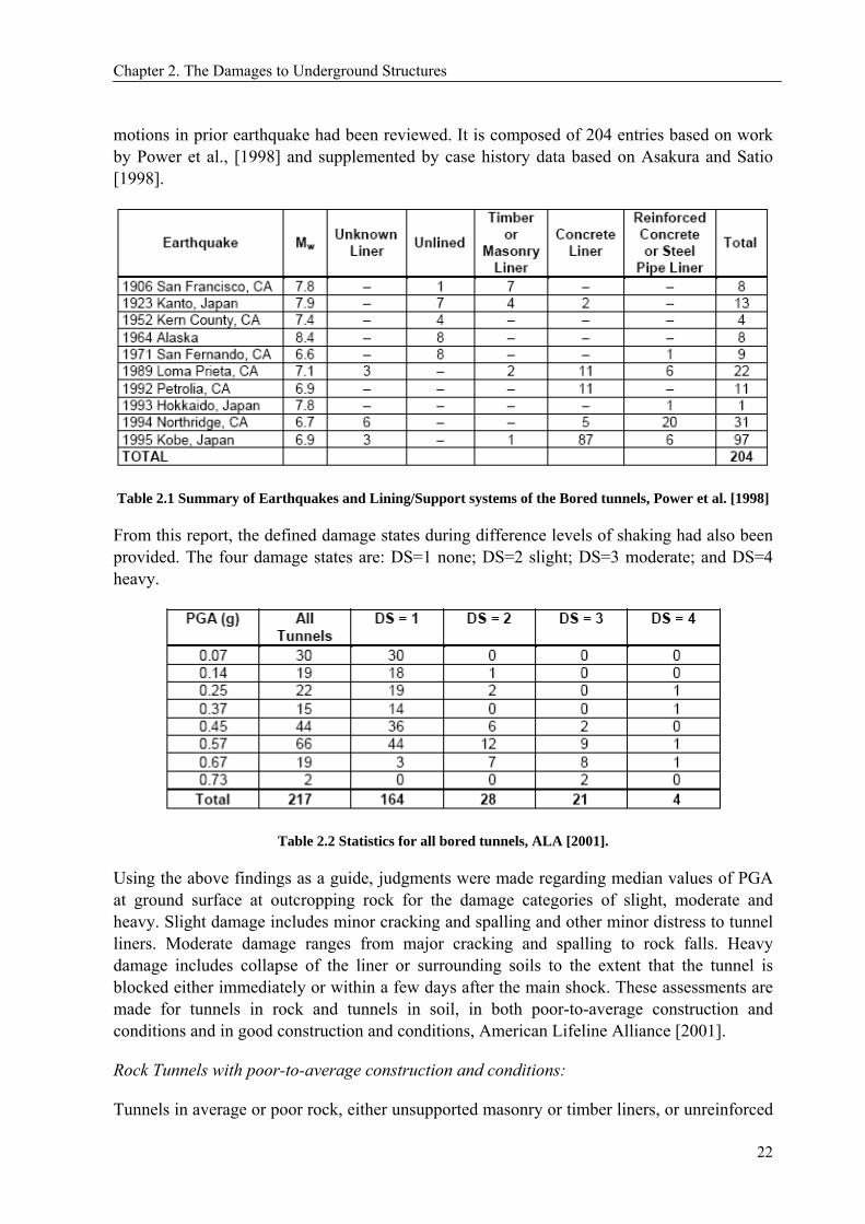
motions in prior earthquake had been reviewed. It is composed of 204 entries based on work by Power et al., [1998] and supplemented by case history data based on Asakura and Satio [1998].
Table 2.1 Summary of Earthquakes and Lining/Support systems of the Bored tunnels, Power et al. [1998]
From this report, the defined damage states during difference levels of shaking had also been provided. The four damage states are: DS=1 none; DS=2 slight; DS=3 moderate; and DS=4 heavy.
Table 2.2 Statistics for all bored tunnels, ALA [2001].
Using the above findings as a guide, judgments were made regarding median values of PGA at ground surface at outcropping rock for the damage categories of slight, moderate and heavy. Slight damage includes minor cracking and spalling and other minor distress to tunnel liners. Moderate damage ranges from major cracking and spalling to rock falls. Heavy damage includes collapse of the liner or surrounding soils to the extent that the tunnel is blocked either immediately or within a few days after the main shock. These assessments are made for tunnels in rock and tunnels in soil, in both poor-to-average construction and conditions and in good construction and conditions, American Lifeline Alliance [2001].
Rock Tunnels with poor-to-average construction and conditions:
Tunnels in average or poor rock, either unsupported masonry or timber liners, or unreinforced
22

Chapter 2. The Damages to Underground Structures
concrete with frequent voids behind lining and/or weak concrete.
Rock Tunnels with good construction and conditions:
Tunnels in very sound rock and designed for geologic conditions (e.g., special support such as rock bolts or stronger liners in weak zones); unreinforced, strong concrete liners with contact grouting to assure continuous contact with rock; average rock; or tunnels with reinforced concrete or steel liners with contact grouting.
Alluvial (Soil) and Cut and Cover Tunnels with poor to average construction:
Tunnels that are bored or cut and cover box-type tunnels and include tunnels with masonry, timber or unreinforced concrete liners, or any liner in poor contact with the soil. These also include cut and cover box tunnels not designed for racking mode of deformation.
Alluvial (Soil) and Cut and Cover Tunnels with good construction:
Tunnels designed for seismic loading, including racking mode of deformation for cut and cover box tunnels. These also include tunnels with reinforced strong concrete or steel liners in bored tunnels in good contact with soil.
Table 2.3 Tunnel Fragility-Median PGAs-Ground shaking hazard only, ALA [2001].
The magnitudes of the median fragilities are about the same for tunnels of good quality construction and somewhat lower for tunnels of lower quality construction. The heavy damage state is provided only for tunnels with poor-to-average conditions. From the observation of this database, no heavy damage has occurred to well-constructed tunnels in good ground conditions.
2.4 Lesson learns from the past damages The following general observation can be made regarding the seismic performance of underground structures.
2.4.1 Geological settings Mountain tunnels in rock and lined without material and structural defects are less affected by an earthquake even if it is very large. Seismic waves propagate faster in hard and dense materials, and thus less energy will be released at places where the tunnels lie in ground that is harder than the tunnel structure, meaning that such tunnels will tend to deform with the
23

Chapter 2. The Damages to Underground Structures
ground and suffer less damage. On the other hand, if the tunnels lie in relatively weaker ground they will absorb larger amounts of energy and thus suffer greater damage. Concrete linings can particularly be damaged easily by ground displacement or ground squeeze where soft and hard grounds meet, as soft and hard grounds behave differently during earthquakes, Hashash, et al. [2001].
2.4.2 Concrete lining Okamoto [1973] reviewed damages to railway tunnels in 1923 Kanto earthquake. Based on observed damages he concluded that there is a certain correlation between lining thickness and damage, i.e. earthquake damage was greater in sections which thick lining than thin ones as shown in the following:
Lining Thickness (cm) 57.1 45.7 34.3 22.9
Damage Rate 80 % 55 % 11 % 0 %
Also, during the Kita-Minto earthquake, the rate of damage to waterway tunnels for hydroelectric power generation is as high as 82 % for lining thickness of 40 cm, and only 16 % for thickness of 20 cm. The damage ratios are compared only be geological classification without consideration of lining thickness, the rate is progressively reduced in the order of soil or soil and gravel, rock with joints, soft rock, and hard rock as shown in following:
Type of soil Hard rock Soft rock Rock with joints Soil or Soil & Gravel
Damage Rate 16 % 40 % 44 % 61 %
The damage characteristics described above indicates the rate of damage is higher the poorer the geology of the ground and also higher the thicker the lining. This shows the importance of geological settings which can not be overcome by merely increasing the lining thickness, Okamoto [1973].
Concrete linings can particularly be damaged easily by ground displacement or ground squeeze where soft and hard grounds meet, as soft and hard grounds behave differently during earthquakes. Any unfavorable events such as cave-in or collapse during tunneling would extend the plastic zone around the tunnel, weaken the surrounding rock and cause excessive vibration when seismic waves pass through. In addition, if the ground has previously experienced vertical stress from loosening, plastic stress owing to squeezing, inclined stress or any other weakening processes, tunnels in these areas will suffer greater damage to their concrete linings during an earthquake [Wang et al., 2001].
Tunnels are more stable under a symmetric load, which improves ground-lining interaction. Improving the tunnel lining by placing thicker and stiffer sections without stabilizing surrounding poor ground may result in excess seismic forces in the lining. Backfilling with non-cyclically mobile material and rock-stabilizing measures may improve the safety and stability of shallow tunnels, Hashash, et al. [2001].
2.4.3 Distance effect The intensity of seismic force experienced by each tunnel differs owing to their different distances from the displaced fault zone and the direction from the epicenter of the earthquake.
24

Chapter 2. The Damages to Underground Structures
Seismic waves propagate in the ground and lose energy because of dispersion and ground resistance, causing tunnels to be under greater seismic forces if they are closer to the displaced fault zone or the epicenter. The near-fault effect should be considered in this short distance case.
2.4.4 Overburden depth The distance to the ground surface also influences the seismic effect. When seismic waves reach the ground surface, they release energy due to reflection or refraction, and thus tunnels near the surface, and especially those near slope faces, will absorb a greater seismic energy. High shaking intensity is also due to the lower stiffness of the soils and the site amplification effect. The frequencies of damage reports decrease with depth, which is attributed to the lack of surface waves, lower acceleration with depth, and increased strength of the rock with depth. However, far more facilities exist at shallower depth a fact that may induce considerable bias, [Sharma and Judd, 1991].
2.4.5 Slope stability Damage at and near tunnel portals may be significant due to slope instability. The primary failure mode tends to be slope failure. Particular caution must be taken if the portal also acts as a retaining wall [St. John and Zahrah, 1987].
2.4.6 Duration of earthquake Duration of strong-motion shaking during earthquakes is of utmost importance because it may cause fatigue and therefore, large deformations, [Hashash, et al, 2001].
2.4.7 Frequency-content effect High frequency motions may explain the local spalling of rock or concrete along planes of weakness. These frequencies, which rapidly attenuate with distance, may be expected mainly at small distances from the causative fault, [Hashash, et al, 2001].
2.4.8 Peak ground motion parameters Damage may be related to peak ground velocity based on the magnitude and rupture distance of the affected earthquake, [Hashash, et al, 2001].
2.4.9 Near-fault effect For the near-fault zone, the directivity and fling step effects are obviously dominated the tunnel responses. The underground structural design should also include the effect of high intensity ground motion at intermediate to long period pulse.
25

Chapter 3. Seismic Design and Analysis Procedures for Underground Structures
3 SEISMIC DESIGN AND ANALYSIS PROCEDURES FOR
UNDERGROUND STRUCTURES
3.1 Seismic behaviors of underground structures In general, seismic design loads for underground structures are characterized in terms of the deformations and strains imposed on the structure by the surrounding ground, often due to the interaction between the two. For most underground structures, the inertia of the surrounding soil is large relative to the inertia of the structure. The response of a tunnel is neither resonance in the ground nor dominated by the inertial properties of the tunnel structure itself, but it conforms to the surrounding ground response, Kawashima [2000]. The author also gives two major reasons for this phenomenon. First, the mass effect is generally small in an underground structure, because the gross unit weight of an underground structure is generally 10.5 – 11 kN/m3 while the unit weight of the surrounding soils is generally in the range of 14 – 18 kN/m3. Second, the damping of an underground structure is very high due to the radiation of energy from the structure to the surrounding ground. In contrast, surface structures are designed for the inertial forces caused by ground accelerations.
The comparison between underground and on ground structure behaviors also proves the previous assumptions. Figure. 3.1 shows the peak response acceleration of the on ground structure is 0.77g and this is larger than the acceleration of 0.6g at the ground surface; this difference is caused by the amplified effect of the on ground structural response. On the other hand, the response acceleration of the underground structure is quite close in both frequency content and peak value to the ground acceleration at the same depth as the underground structure, Kawashima [2000].
26

Chapter 3. Seismic Design and Analysis Procedures for Underground Structures
Figure 3.1 Acceleration response of Underground and On-ground structures, [Kawashima, 2000]
The major factors influencing shaking damage include: [Dowding and Rozen, 1978; St. John and Zahrah, 1987]
• The shape, dimensions, and depth of the structure
• The properties of the surrounding soil or rock
• The properties of the structure
• The severity of the ground shaking, e.g. duration, PGA, PGV, and frequency effects.
The general behavior of the linear tunnel is similar to that of an elastic beam subject to deformation or strains imposed by the surrounding ground. Owen and Scholl [1981] express the response of underground structures to seismic motions into three types:
(1) Axial extension and compression
27

Chapter 3. Seismic Design and Analysis Procedures for Underground Structures
Axial deformations in tunnels are generated by the components of seismic waves that produce motions parallel to the axis of the tunnel and cause alternating compression and tension. The design of a tunnel lining to accommodate axial deformations generally concentrates on the direction along the tunnel axis, Wang [1993]. This type of deformation is slightly complex since there will be some interaction between the structure and the ground. This interaction would be more important if the ground is soft and shear stress transfer between the ground and the structure is limited by the interface shear strength, Hashash et al. [2001].
Figure 3.2 Axial deformation along the tunnel, Wang [1993].
(2) Curvature deformation or longitudinal bending
Bending deformations are caused by the components of seismic waves producing particle motions perpendicular to the longitudinal axis. The design and analysis of bending deformations are also in the longitudinal direction along the tunnel axis, Wang [1993].
Figure 3.3 Bending deformation along the tunnel, Wang [1993].
(3) Ovaling deformations
Ovaling deformation in a tunnel structure develops when shear waves propagate normal or nearly normal to the tunnel axis, resulting in a distortion of the cross-sectional shape of the tunnel lining. Design considerations for this type of deformation are in the transverse direction. The general behavior of the lining may be simulated as a buried structure subject to ground deformations under a two-dimensional plane-strain condition, Hashash et al. [2001].
Ovaling deformations may be caused by vertically, horizontally or obliquely propagating seismic waves of any type. Many previous studies have suggested, however, that the vertically propagating shear wave is the predominant form of earthquake loading that governs the tunnel lining design against ovaling. The following reasons are given, Wang [1993]:
28

Chapter 3. Seismic Design and Analysis Procedures for Underground Structures
- Ground motion in the vertical direction is generally considered less severe than its horizontal component. Typically, vertical ground motion parameters are assumed to be 1/2 to 2/3 of the horizontal ones. (Note that a vertically propagating shear wave causes the ground to shake in the horizontal direction.) This relation is based on observation of California earthquakes, which are most commonly of the strike-slip variety in which horizontal motion predominates, Wang [1993].
For thrust faults, in which one rock block overrides another, vertical effects may equal or exceed the horizontal ones. The effects of thrust faulting are usually more localized, however, than those of the strike-slip faulting, and they are attenuated more rapidly with distance from the focus, Wang [1993].
- For tunnels embedded in soils or weak media, the horizontal motion associated with vertically propagating shear waves tends to be amplified. In contrast, the ground strains due to horizontally propagating waves are found to be strongly influenced by the ground strains in the rock beneath. Generally, the resulting strains are smaller than those calculated using the properties of the soils, Wang [1993].
Figure 3.4 Ovaling deformation of a circular cross section [Owen and Scholl, 1981]
3.2 Design and analysis methods Design methods have been developed to estimate seismic loads on underground structures. These methods include free-field deformation motion, which the ground deformation/strains caused by the travelling seismic waves without the structure being present is imposed on the underground structure, as well as dynamic soil-structure interaction analysis.
3.2.1 The free field deformation method This simplest method, the quasi-static method without soil-structure interaction, assumes conservatively that the structure is flexible enough to follow the deformations of the surrounding grounds. Thus by using the maximum values of amplitude and wavelength of the soil seismic deformation, the maximum structural strains can be determined. This approach shows satisfactory results when low levels of shaking are anticipated or the underground structure stiffness is similar to the surrounding ground.
29

Chapter 3. Seismic Design and Analysis Procedures for Underground Structures
However, the applicability of this approach is quite limited, since it may overestimate or underestimate structure deformations depending on the rigidity of the structure relative to the ground. In many cases, especially in soft soils, this method gives overly conservative designs because of free-field ground distortions in soft soils are generally large. For example, rectangular box structures in soft soils are typically designed with stiff configurations to resist static loads and are therefore, less tolerant to racking distortions, Hwang and Lysmer, [1981]. On the other hand, when the tunnel structure is flexible relative to the surrounding ground, this method may also underestimate the seismic responses of the structure. Soil-structure interaction effects have to be included for the design of such structures Wang [1993].
The free-field deformation method, nevertheless, has been used on many significant projects, including the San Francisco BART stations and tunnels, Kuesel [1969] and the Los Angeles Metro, Monsees and Merritt [1991], while Sakurai and Takahashi [1969] apply it to underground pipelines. The newly built Daikai station in Kobe was also designed in this criterion. Kuesel found that, in most cases, if a structure can absorb free-field soil distortions elastically, no special seismic provisions are necessary.
(1) Closed form elastic solutions
This simplified method assumes the seismic wave field to be that of plane waves with the same amplitudes at all locations along the tunnel, differing only in their arrival time. Wave scattering and complex three-dimensional wave propagation, which can lead to differences in wave amplitudes along the tunnel are neglected, although ground motion incoherence tends to increase the strains and stresses in the longitudinal direction. Then, results of analyses based on plane wave assumptions should be interpreted with care, Power et al. [1996].
Newmark [1968] and Kuesel [1969] proposed a simplified method for calculating free-field ground strains caused by a harmonic wave propagating at a given angle of incidence in a homogeneous, isotropic, elastic medium (Figure 3.5). The most critical incidence angle yielding maximum strain is typically used as a safety measure against the uncertainties of earthquake prediction. Newmark’s approach provides an order of magnitude estimate of wave-induced strains while requiring a minimal input, making it useful as both an initial design tool and a method of design verification [Wang 1993; Hashash et al. 2001].
30

Chapter 3. Seismic Design and Analysis Procedures for Underground Structures
Figure 3.5 Geometry of a sinusoidal shear wave oblique to axis of tunnel, Wang [1993]
St. John and Zahrah [1987] used Newmarks’s approach to develop solutions for free-field longitudinal, normal, and shear strains due to compression (P-wave), shear (S-wave) and Rayleigh waves Table 3.1. However, it is generally considered that the P-wave induced response would not control the design. It is also difficult to determine which type of wave will dominate due to the complex nature of the characteristics associated with different wave types. Generally, strains produced by Rayleigh waves may govern only when the site is at a large distance from the earthquake source and the structure is built at shallow depth, Wang [1993].
31

Chapter 3. Seismic Design and Analysis Procedures for Underground Structures
Strain and curvature due to body and surface waves, St. John and Zahrah [1987]
Wave type Longitudinal strain Normal strain Shear strain Curvature
P-wave 2cosPl
P
VC
ε φ= 2sinPn
P
VC
ε φ= sin cosP
P
VC
γ φ φ= 22 sin cosP
P
aKC
φ φ=
for 0Plm
P
VC
ε φ= = o for 90Pnm
P
VC
ε φ= = o for 452
Pm
P
VC
γ φ= = o '20.385 for 35 16P
mP
aKC
φ= = o
S-wave sin cosSl
S
VC
ε φ φ= sin cosSn
S
VC
ε φ φ= 2cosS
S
VC
γ φ= 32 cosS
S
aKC
φ=
for 452
Slm
S
VC
ε φ= = o for 452
Snm
S
VC
ε φ= = o for 0Sm
S
VC
γ φ= = o 2 for 0Sm
S
aKC
φ= = o
Rayleigh wave
2cosRPl
R
VC
ε φ= 2sinRPn
R
VC
ε φ= sin cosRP
R
VC
γ φ φ= 22 sin cosRP
R
aKC
φ φ= Compressional
for 0RPlm
R
VC
ε φ= = o for 90RPnm
R
VC
ε φ= = o for 452
RPm
R
VC
γ φ= = o '20.385 for 35 16RP
mR
aKC
φ= = o component
sinRSn
R
VC
ε φ= cosRS
R
VC
γ φ= 22 cosRS
R
aKC
φ= Shear
component
for 90RSnm
R
VC
ε φ= = o for 0RSm
R
VC
γ φ= = o 2 for 0RSm
R
aKC
φ= = o
Table 3.1 Strains and curvatures due to body and surface waves
32

Chapter 3. Seismic Design and Analysis Procedures for Underground Structures
Notation:
The Poisson's ratio and dynamic modulus of a soil deposit can be computed from measured P-wave and S-wave propagation velocities in an elastic medium:
The Poisson’s ratio
2
2
212 1
p
s
p
s
CC
CC
ν−
=−
⎛ ⎞⎜ ⎟⎝ ⎠⎛ ⎞⎜ ⎟⎝ ⎠
; Young’s modulus ( ) ( )( )
2 1 1 21pE Cν ν
ρν
+ −=
−; and Shear
modulus 2sG Cρ= ⋅ , respectively.
where:
r: radius of circular tunnel or half height of a rectangular tunnel
aP: peak particle acceleration associated with P wave
aS: peak particle acceleration associated with S wave
aRP: peak particle acceleration associated with Rayleigh wave, compressional component
aRS: peak particle acceleration associated with Rayleigh wave, shear component
Φ: angle of incidence of wave with respect to tunnel axis
Vp: peak particle velocity associated with P wave
Cp: apparent velocity of P wave propagation
Vs: peak particle velocity associated with S wave
Cs: apparent velocity of S wave propagation
VRP: peak particle velocity associated with Rayleigh Wave, compressional component
VRS: peak particle velocity associated with Rayleigh Wave, shear component
CR: apparent velocity of Rayleigh wave propagation
ρ : mass density
Combined axial and curvature deformations can be obtained by treating the tunnel as an elastic beam. Using beam theory, total free-field axial strains, εab, are found by combining the longitudinal strains generated by axial and bending deformations, Power et al. [1996]
22cos sin cosab P P
P P
V arC C
2ε φ φ⎡ ⎤
= +⎢⎣ ⎦
φ⎥ for P-waves (3.1)
33

Chapter 3. Seismic Design and Analysis Procedures for Underground Structures
32sin cos cosab S S
S S
V arC C
ε φ φ φ⎡ ⎤
= +⎢⎣ ⎦
⎥ for S-waves (3.2)
22cos sin cosab R R
R R
V arC C
2ε φ φ⎡ ⎤
= +⎢⎣ ⎦
φ⎥ for Rayleigh-waves (compressional component) (3.3)
Application of the strain equation in Table 3.1 requires knowledge of:
- The apparent wave propagation velocity
- The peak particle velocity
- The peak particle acceleration
The peak particle velocity and acceleration can be established through empirical methods, field measurements, or site-specific seismic exposure studies. The apparent wave propagation velocity in rock can be determined with reasonable confidence from in-situ and laboratory tests. Estimating the apparent wave propagation velocity in soil overburden presents the major difficulty. Previous studies have shown that, except possibly for vertically propagating shear waves, the use of soil properties in deriving the wave velocity in soil overburden may be overly conservative. Free-field ground deformations and velocities due to a seismic event should then be estimated using site specific response analysis that accounts for local geology.
The contribution of bending deformation to axial strain increases as the radius of the tunnel increases. However, calculations using the equations shown in Table 3.1 indicate that the bending component of strain is, in general, relatively small compared to axial strains for tunnels under seismic loading. The cyclic nature of the axial strains should also be noted. Although a tunnel lining may crack in tension, this cracking is usually transient due to the cyclic nature of the incident waves. The reinforcing steel in the lining may close these cracks at the end of the shaking, provided there is no permanent ground deformation and the steel has not yielded, Hashash et at. [2001]. Even unreinforced concrete linings are considered adequate as long as the cracks are small, uniformly distributed, and do not adversely affect the performance of the lining, Wang [1993]. According to this method moment and forces generated in tunnel lining are in the following form:
2
31 1
2 cos sin/ cos
M E I DL Lπ θ 2π
θ⎛ ⎞ ⎛= ⋅ ⋅ ⋅ ⋅ ⋅⎜ ⎟ ⎜⎝ ⎠ ⎝
⎞⎟⎠
(3.4)
3
41 1
2 cos cos/ cos
V E I DL Lπ θ 2π
θ⎛ ⎞ ⎛= ⋅ ⋅ ⋅ ⋅ ⋅⎜ ⎟ ⎜⎝ ⎠ ⎝
⎞⎟⎠
(3.5)
1 12 2cos sin cos
/ cosQ E A D
L Lπ πθ θ
θ⎛ ⎞ ⎛= ⋅ ⋅ ⋅ ⋅ ⋅ ⋅⎜ ⎟ ⎜⎝ ⎠ ⎝
⎞⎟⎠
(3.6)
where M, bending moment; V, shear force; Q, axial force; θ, angle of wave impact; I1, moment of inertia of tunnel lining; E1, modulus of elasticity of lining material; D, amplitude of sine wave; L, shear wavelength; and A1, section area of lining.
34

Chapter 3. Seismic Design and Analysis Procedures for Underground Structures
(2) Ovaling deformation of circular tunnels
Ground shear distortions can be defined in two ways, as shown in Figure 3.8: (1) Non-perforated ground; and (2) Perforated ground. Typically two-dimensional, plane strain conditions are considered. In the non-perforated ground, the maximum diametric strain εd is a function only of the maximum free-field shear strain γmax:
max
2dd
dγε Δ
= = ± (3.7)
where; d is the diameter of the opening. The diametric strain in a perforated ground is related to the Poisson’s ratio of the medium:
(max2 1dd
d)ε γ νΔ
= = ± − (3.8)
(a) (b)
(a) Non-perforated medium (b) Perforated medium
Figure 3.6 Free-field shear distortion of ground Wang [1993]
Both equations assume that there is no liner, therefore ignoring structure-ground interaction. The perforated ground yields a much greater distortion than the non-perforated ground, by a factor of two to three. Results with the perforated ground may provide a reasonable distortion criterion for a soft lining, while the non-perforated results may be appropriate when the lining stiffness is similar to that of the ground. A lining with large relative stiffness should experience distortions much smaller than those given by Eq. (3.8) Perforated, Wang [1993].
Okamoto [1973] also developed the analytical solution using the theory of elastic waves to the dynamics of a tunnel to investigate the effect of lining thickness. The stress around a hole subjected to shear wave coming from one side was calculated. In this case shear waves and longitudinal waves are reflected from the surface of the hole, and a stress concentration is produced around the hole, while in the tunnel lining a reaction force to the reflection of seismic waves acts as seismic force.
35

Chapter 3. Seismic Design and Analysis Procedures for Underground Structures
Figure 3.7 The interaction between elastic waves and tunnel lining
As indicated in Figure 3.7, the calculations were made for sinusoidal shear waves, ( ){ }exp /a ip t x β+ , propagating along the x axis. The result shows that the following seismic
force acts normal to the surface of the lining when the diameter of the hole is small in relation to the wavelength of the earthquake motion:
0 sin 2rr rr θ= (3.9)
.The maximum seismic load is given by the following equation:
3
0
0 3
6
16c
havrrr
g hE rβ
ρβ
⎛ ⎞⎜ ⎟⎝ ⎠=
⎛ ⎞+ ⎜ ⎟⎝ ⎠
(3.10)
where
a is the amplitude of incident seismic wave;
rr is the intensity of seismic load per unit width of lining acting perpendicular on lining
surface;
rr0 is the maximum value of rr;
r is the radius of tunnel;
h is the thickness of lining;
ρ is the unit weight of soil;
β is the propagation velocity of shear wave;
v0 is the velocity amplitude of seismic wave; and
36

Chapter 3. Seismic Design and Analysis Procedures for Underground Structures
Ec is the Young’s modulus of lining concrete.
Bending moment is produced in the lining and the maximum fiber stress is given by the following equation:
0
3
12
16c
havr
g hE r
σ θβ
ρβ
=⎛ ⎞+ ⎜ ⎟⎝ ⎠
(3.11)
According to this equation, both rr and σ are proportional to v0. Therefore, it is the peak ground velocity of the earthquake motion which affects the stress of the lining.
2 2/ , /m kg cm rr t mσ ⎡ ⎤ ⎡⎣ ⎦ ⎣ ⎤⎦
Figure 3.8 Relationship between stress and thickness of tunnel lining, Okamoto[1973]
Form previous equations, the seismic stresses produced in the lining depending on the lining thickness. Figure 3.8 shows the seismic forces acting on the lining and the seismic stresses produced thereby for cases of various earthquake wave propagation velocities. According to this, the seismic load acting on the lining and the seismic stress increase with increased lining thickness. In general, increased thickness tends to have a detrimental effect on the lining. Some general conclusion can be given as:
(a) The seismic load acting on the lining was increased and the seismic stress also became greater the slower the seismic wave propagation velocity
(b) With the exception of very slow seismic wave propagation velocity, the seismic load and seismic stress were increased with increased lining thickness.
(c) However, when the propagation velocity of seismic waves was extremely slow in a range above a certain lining thickness, increase in the lining thickness reduced seismic stress. This reduction in seismic stress was not, however, very great considering the increase in lining thickness.
3.2.2 The soil-structure interaction method A pseudo-static analysis method is commonly used to account for soil-structure interaction
37

Chapter 3. Seismic Design and Analysis Procedures for Underground Structures
effects. However, the pseudo static approach may be valid for weak ground motion where deformations are elastic.
In this approach it is assumed that the presence of an underground structure modifies the deformations of the ground around the structure, and thus the free-field ground deformations are not experienced by the structure [Wang, 1993; Penzien and Wu, 1998; Penzien, 2000; and Hashash et al. 2001]. The ground and the underground structure have a complex interaction during seismic motions. In general, when an underground structure is stiffer than its surrounding soils, the structure resists, rather than conforms to the deformations imposed by the ground. On the other hand, when an underground structure is more flexible than its surrounding ground, the deformations of the ground surrounding the structure may be larger than those of the free-field ground. Relative stiffness (stiffness ratio) between an underground structure and the surrounding ground plays a key role in the response of the structure.
(1) Elastic solutions of longitudinal deformations for circular tunnels
The beam-on-elastic foundation approach is used to model pseudo-static ground structure interaction effects. The solutions ignore dynamic inertial interaction effects. Under seismic loading, the cross-section of a tunnel will experience axial bending and shear strains due to free field axial, curvature, and shear deformations (Figure 3.9). St. John and Zahrah [1987] proposed that the maximum structural strains are caused by a wave at an incident angle of 45º. The maximum axial strain εa
max used by a 45º incident shear wave (Figure 3.7) is:
max 2
2
422
a
l cl c
a
AfLL
E AE AK L
π
επ
⎛ ⎞⎜ ⎟⎝ ⎠= ≤
⎛ ⎞+ ⎜ ⎟⎝ ⎠
(3.12)
where
L : Wavelength of an ideal sinusoidal shear wave
Ka : Longitudinal spring coefficient of ground medium (see Eq. 11); in units of
force per unit deformation per unit length
A : Free-field ground displacement response amplitude for an ideal sinusoidal
shear wave
Ac : Cross-sectional area of tunnel lining
El : Elastic modulus of the tunnel lining
f : Maximum friction force per unit length between tunnel and surrounding soil
Eq. 3.7 states that the maximum axial strain shall be smaller than the one induced by the
38

Chapter 3. Seismic Design and Analysis Procedures for Underground Structures
maximum shear force that can be developed between tunnel and surrounding soil. The maximum friction shear is dependent on the roughness of the ground-tunnel interface and the normal force applied to the tunnel from the ground.
Figure 3.9 Induced forces and moments caused by waves propagating along tunnel axis
The maximum bending strain occurs when the incident angle of shear wave is equal to 0º (Figure 3.5):
2
max 4
2
21
b
l c
l
AL r
E IK L
π
επ
⎛ ⎞⎜ ⎟⎝ ⎠=
⎛ ⎞+ ⎜ ⎟⎝ ⎠
(3.13)
Ic: moment of inertia of the tunnel section
Kl: transverse spring coefficient of the ground medium (see Eq. 3.18); in force per unit
deformation per unit length of tunnel
r: radius of circular tunnel or half height of a rectangular tunnel
The maximum shear force on the tunnel cross-section can be written as a function of this maximum bending strain:
3
maxmax 4
22
21
l c bl c
l c
l
E I AE ILV
L rE IK L
πεπ
π
⎛ ⎞⎜ ⎟ ⎛ ⎞⎛ ⎞⎝ ⎠= = ⎜⎜ ⎟
⎝ ⎠⎛ ⎞ ⎝ ⎠+ ⎜ ⎟⎝ ⎠
⎟ (3.14)
The maximum bending moment is:
39

Chapter 3. Seismic Design and Analysis Procedures for Underground Structures
2
max 4
2
21
l c
l c
l
E I ALME IK L
π
π
⎛ ⎞⎜ ⎟⎝ ⎠=
⎛ ⎞+ ⎜ ⎟⎝ ⎠
(3.15)
and the maximum axial force is (from Eq. 3.12):
max 2
2
22
l c
l c
a
E I ALQE IK L
π
π
⎛ ⎞⎜ ⎟⎝ ⎠=
⎛ ⎞+ ⎜ ⎟⎝ ⎠
(3.16)
A conservative estimate of the total maximum axial strain is obtained by combining the axial and bending strains since both the liner and the ground are assumed as linear elastic, Power et al., [1996]:
max max maxab a bε ε ε= + (3.17)
Note that in the above equations, the interaction between ground and structure is modeled by including springs with the spring coefficients Ka and Kl for longitudinal and transverse soil response. St. John and Zahrah [1987] suggested that the spring coefficients Ka and Kl are functions of the incident wavelength:
( )( )
16 13 4a lG dK K
Lπ ν
ν−
= =−
(3.18)
where G is the shear modulus and ν is the Poisson’s ratio of the ground; d is the diameter of circular tunnels or the height of rectangular tunnels; and L is the incident wavelength.
Wang [1993] indicated that the springs differ from those of a conventional beam analysis on an elastic foundation. Not only must the coefficients be representative of the dynamic modulus of the ground, but the derivation of these constants must consider the fact that the seismic loading is alternately positive and negative due to the sinusoidal wave.
The input wavelengths for underground structure design have been investigated by a number of researchers. The incident wavelength of a ground motion may be estimated as:
sL T C= ⋅ (3.19)
where T is the natural period of a shear wave in the soil deposits and Cs is the shear wave velocity. Idriss and Seed [1968] recommended that:
4
s
hTC
= (3.20)
40

Chapter 3. Seismic Design and Analysis Procedures for Underground Structures
where h is the thickness of the soil deposit.
The ground displacement response amplitude A, in Eqs (3.12) through (3.16), represents the spatial variation of ground motions along a horizontal alignment and should be derived by site-specific subsurface conditions. The displacement amplitude generally increases with increasing wavelength. In case of a sinusoidal shear wave with a displacement amplitude A and a wavelength L, the displacement amplitude A can be calculated from the following equations:
For free-field axial strains:
2 sin coss
s
VAL Cπ φ φ= (3.21)
For free-field bending strains:
2
32
4 coss
s
aACL
π φ= (3.22)
For a sinusoidal compression wave with a displacement amplitude A and a wavelength L, the displacement amplitude A can be calculated from the following equations:
For free-field axial strains:
22 cosp
p
VAL Cπ φ= (3.23)
For free-field bending strains:
2
22
4 sin cosp
p
aACL
π φ φ= (3.24)
(2) Ovaling deformations of circular tunnels
Peck et al. [1972] characterized tunnel liners into two groups: flexible liners and rigid liners. A liner is said to be "flexible" if it interacts with the ground in a way that the pressure distribution on the liner and the corresponding deflected shape result in negligible bending moments in the lining. A "rigid" liner is a liner which deflects insignificantly under the loads imposed by the ground; and thus it has to support large bending moments.
Actual tunnel linings are neither perfectly flexible nor perfectly rigid. A tunnel that may be rigid in a soft ground may behave as a flexible liner in a very stiff ground. In order to quantitatively describe the relative stiffness between tunnels and ground, based on earlier work by Burns and Richard [1964] and Hoeg [1968], Peck et al. [1972] proposed that the relative stiffness of a tunnel-ground system can be divided into two separate and distinct types. The first type is extensional stiffness, which is a measure of the equal uniform pressure
41

Chapter 3. Seismic Design and Analysis Procedures for Underground Structures
to cause a unit diametric strain of the tunnel without changing the shape of the tunnel. The second type is flexural stiffness, which is a measure of the non-uniform pressure to cause a unit diametric strain resulting in a change in shape or an ovaling of the tunnel. The relative stiffness between the tunnel and surrounding ground is hence characterized by two dimensionless ratios designated as the compressibility ratio and flexibility ratio (C and F).
The compressibility ratio, a measure of the extensional stiffness of the ground to that of the liner, is obtained by considering an infinite, elastic, homogeneous and isotropic ground subjected to a uniform external pressure. The compressibility ratio is equal to the ratio between the pressure required to cause a unit diametric strain (contraction) of the free-field ground and the pressure required to cause a unit diametric strain (contraction) of the liner. Note that in order to obtain the diametric strain of the free-field ground, a circle with its size identical to the liner is assumed. The compressibility ratio can be expressed as:
( )
( )( )
21
1 1 2l
l
E rC
E t
ν
ν ν
−=
+ − (3.25)
where E is the Young's modulus of the ground; v is the Poisson's ratio of the ground; I is the moment of inertia of the tunnel lining per unit width; r is the radius of the tunnel; and t is the thickness of the tunnel lining.
The flexibility ratio, a measure of the flexural stiffness of the ground to that of the liner, is obtained by considering an infinite, elastic, homogeneous and isotropic ground subjected to a pure shear loading. The flexibility ratio is equal to the ratio between the shear stress required to cause a unit diametric strain (ovaling) of the free-field ground and the shear stress required to cause a unit diametric strain (ovaling) of the liner. Note that in order to obtain the diametric strain of the free-field ground, a circle with size identical to the liner is assumed. The flexibility ratio is:
( )
( )
2 31
6 1l
l
E rF
E I
ν
ν
−=
+ (3.26)
It is often suggested that the flexibility ratio is the most important because it is related to the ability of the lining to resist distortion imposed by the ground. Burns and Richard [1964] have shown that the forces and deformations of ground and structure depend on (1) the compressibility ratio, C; (2) the flexibility ratio, F; and (3) the slippage at the interface between the ground and the liner. The interface between ground and support has often been assumed to be frictional, i.e. the shear stress and normal stress developed at the interface follow the Coulomb friction law. In other words, the maximum shear stress at the interface is equal to the normal stress times the friction coefficient between ground and support. Two extreme cases are considered: full-slip and no-slip.
The full-slip case assumes that the friction coefficient is zero and no shear force develops at the interface. The ground may detach from the tunnel during an earthquake. In the no-slip case, the friction coefficient is such that the ground and structure are tied together. The ground
42

Chapter 3. Seismic Design and Analysis Procedures for Underground Structures
and structure cannot be separated. Actual conditions may be in between these two extreme cases. However, due to the complexity of the problem, most of the work has focused on either full-slip or no-slip interface conditions.
- Full-slip conditions
Peck et a1. [1972] provided closed-form solutions for diametric strain εd, thrust T, and bending moment M, for the full-slip case under static loading conditions, i.e. tunnels under overburden and lateral earth pressures. The displacements and forces are functions of the compressibility ratio C, flexibility ratio F and the in-situ overburden pressure of the soil γ, H.
At the crown and invert of a circular tunnel:
( )( ) ( )0 01 2 11 1 12 3 1 2
ld l
C
Hrd K b C K b Fd M
γ νε νν
Δ −2
⎡ ⎤= = − + + −⎢ ⎥−⎣ ⎦ (3.27)
( ) ( )0 1 0 21 11 12 3tT Hr K b K bγ ⎡ ⎤= + − −⎢ ⎥⎣ ⎦
(3.28)
( )( ) ( )0 1 0 21 2 11 1 12 3 1 2
td
C
Hrd K b C K b Fd M
γ νε νν
Δ −⎡ ⎤= = − + + −⎢ ⎥−⎣ ⎦ (3.29)
( )20 2
1 16 tM Hr K bγ ⎡ ⎤= −⎣ ⎦ (3.30)
At the springline of a circular tunnel;
( )( ) ( )0 01 2 11 1 12 3 1 2
td l
C
Hrd K b C K b Fd M
γ νε νν
Δ −2
⎡ ⎤= = − + − −⎢ ⎥−⎣ ⎦ (3.31)
( ) ( )0 1 0 21 11 12 3tT Hr K b K bγ ⎡ ⎤= + + −⎢ ⎥⎣ ⎦
(3.32)
( )20 2
1 16 tM Hr K bγ ⎡ ⎤= − −⎣ ⎦ (3.33)
where
γt = Total unit weight of the soil;
Ko= Lateral earth pressure coefficient;
H = Burial depth of the tunnel, measured from the free surface to the center of the tunnel
Mc = Constrained modulus of the soil which is given by:
43

Chapter 3. Seismic Design and Analysis Procedures for Underground Structures
( )( )( )
11 1 2c
EM
νν ν
−=
+ − (3.34)
E = Young’s modulus of the ground;
ν = Poisson’s ratio of the ground;
r = radius of the tunnel;
( )( )( )11 2 1
11 2 1
Cb
Cνν
− −= −
− + (3.35)
and
22 1 2 2 11 3 42 5 6 2 5 6
F FbF F
νν ν
+ − −= + −
+ − + − (3.36)
The solution can be used to obtain deformations and forces due to a shear wave; this can be done by using Ko = -1, which replaces the far field normal stresses σν, and σh = Koσν by a far field shear stress τ, Wang [1993]. After some mathematical manipulations, the diametric strain εd, maximum thrust Tmax, and bending moment Mmax can be presented in the following forms (see Figure 3.10):
Figure 3.10 Induced circumferential forces and moments
caused by waves propagating perpendicular to tunnel axis
1 ma13d
d K Fd xε γΔ
= = ± (3.37)
44

Chapter 3. Seismic Design and Analysis Procedures for Underground Structures
( )max 1 max
16 1
ET K rγν
= ±+
(3.38)
( )
2max 1 max
16 1
EM K r γν
= ±+
(3.39)
where
( )1
12 12 5 6
KF
νν
−=
+ − (3.40)
E and ν are the Young’s modulus and Poisson’s ratio of the ground, respectively; r is the radius of the tunnel; γmax is the maximum free-field ground shear strain and and F is the flexibility ratio defined in Eq. 3.26. Kl is the full-slip lining response coefficient and is determined by Eq. 3.39. The relationship between K1 and F is shown in Figure 3.11, Wang [1993].
Figure 3.11 Lining response coefficients vs. flexibility ratio, full-slip interface, and circular tunnel, Wang
[1993]
45

Chapter 3. Seismic Design and Analysis Procedures for Underground Structures
123
lining
free field
dK F
d −
Δ=
Δ (3.41)
The normalized lining deformation provides an indication of the importance of the flexibility ratio in lining response, Wang [1993]: According to this equation and Figure 3.12, a tunnel lining will deform less than the free field when the flexibility ratio is less than one, i.e. a stiff lining in soft soil. As the flexibility ratio increases, the lining deflects more than the free field and may reach an upper limit equal to the deformations of an opening without support.
Figure 3.12 Normalized lining deflection vs. flexibility ratio, full slip interface, and circular lining, Wang
[1993]
- No-slip conditions
Slip at the interface is only possible for tunnels in soft soils or cases of severe seismic intensity, Hashash et al.[2001]. Full-slip assumptions under simple shear may significantly underestimate the maximum thrust. Hoeg [1968] supported this conclusion and recommend the no-slip assumption is made in assessing the lining response. For no-slip:
46

Chapter 3. Seismic Design and Analysis Procedures for Underground Structures
( )max 2 max 2 max2 1
ET K r K rτ γν
= ± = ±+
(3.42)
where
( ) ( ) ( )
( ) ( )
2
22
11 2 1 2 1 2 221
53 2 1 2 8 6 6 82
F CK
F C C
ν ν ν
ν ν ν ν
⎡ ⎤− − − − − +⎣ ⎦= +
⎡ ⎤⎡ ⎤− + − + − + + −⎣ ⎦ ⎢ ⎥⎣ ⎦ν
(3.43)
K2 is defined as the no-slip lining response coefficient. Expressions for deformations and maximum moment were not provided by the author. The relationship between K2 and C is shown in Figure 3.13, Wang [1993]. The figure shows that seismically-induced thrust increases with decreasing compressibility and flexibility ratios when the Poisson's ratio of the surrounding ground is less than 0.5. As the Poisson's ratio approaches 0.5, the thrust response is independent of compressibility because the soil is considered incompressible, Wang [1993].
47

Chapter 3. Seismic Design and Analysis Procedures for Underground Structures
Figure 3.13 Lining (thrust) response coefficient vs. compressibility ratio, no-slip interface, and circular
tunnel, Wang [1993]
Figure 3.13 (Continued) Lining (thrust) response coefficient vs. compressibility ratio, no-slip interface, and circular tunnel, Wang [1993]
Corigliano et al. [2007] also developed a closed form solution for the pseudo-static analysis of the transversal response. The relationships for the thrust force Q and bending moment M per unit length of tunnel lining for seismic design associated with the no-slip condition between the lining and the surrounding ground are given by the following relations:
( ) max 1 cos 2
2 1 3 4EQ R δ πγν
θ⎡ ⎤⎛ ⎞ ⎛ ⎞= −⎜ ⎟ ⎜ ⎟+⎢ ⎥+ ⎝ ⎠ ⎝ ⎠⎣ ⎦ (3.44)
48

Chapter 3. Seismic Design and Analysis Procedures for Underground Structures
( )
2max
1 1 cos 22 2 1 3 4
EM R δ πγ ε θν
⎡ ⎤⎡ ⎤ ⎛= + + ⎜⎞+ ⎟⎢ ⎥⎢ ⎥+ ⎣ ⎦ ⎝ ⎠⎣ ⎦
(3.45)
where the parameters ε, δ, β, C*, F* are defined by:
( ) ( ){ } ( ) ( ){ } ( )
( ) ( ) ( ){ } ( ) ( )
* * * * * * *
** * * * **
3 / 1 2 3 1 2 1 2 1 2 1 1
31 1 4 2 1 2 1 4 2 1
C F C C C C C
CC C C C C 2F
ν ν ν νε
ν ν ν ν β ν ν ν ν
⎡ ⎤ ⎡ ⎤ ⎡ ⎤ ⎡ ⎤ ⎡− − − − + + − − + − + + −⎣ ⎦ ⎣ ⎦ ⎣ ⎦ ⎣ ⎦ ⎣=⎡ ⎤ ⎡ ⎤ ⎡ ⎤ ⎡− − + − − + + + − + − − +⎣ ⎦ ⎣ ⎦ ⎣ ⎦ ⎣
ν ⎤⎦⎤⎦
(3.46)
( ) ( )
( )
* *
*
1 2 1 4
1 2
C C
C
ν ν νδ
ν
⎡ ⎤ ⎡− − − − +⎣ ⎦ ⎣=⎡ ⎤− +⎣ ⎦
ε⎤⎦
)
(3.47)
( ) ( ) (* *1 4 6 1 2 1C Cβ ν ν ν ν⎡ ⎤ ⎡ ⎤= − + − − + −⎣ ⎦ ⎣ ⎦ (3.48)
( )( )
2*
2
1
1l
l l
ERC
E A
ν
ν
−=
− (3.49)
( )( )
3 2*
2
1
1l
l l
ERF
E I
ν
ν
−=
− (3.50)
where R is the average tunnel radius, A, and Il are area and moment of inertia per unit length of the lining respectively, E, El, ν, and νl are the Young’s modulus and Poisson’s ratio of ground and lining respectively. The parameter C* and F* are the compressibility and flexibility ratios. They represent a measure of the relative stiffness of the ground with respect to the supporting system (i.e. the lining) under a symmetric and antisymmetric loading respectively, Einstein and Schwartz [1979]. Finally γmax is the maximum shear strain (in absolute value) calculated in free-field conditions. Knowing γmax, the imposed stress can be easily computed as follows:
( ) max2 1
Eσ τν
= =+
γ (3.51)
The maximum shear strain is then the key parameter to determine the stress, thrust force, and moment in the tunnel lining.
3.2.3 Numerical methods The analysis of underground structures is complicated due to their interaction with the surrounding soil, especially under dynamic conditions, cut-and-cover structures, mined tunnels with non-circular shapes, and non-uniform properties of circular linings that preclude the use of simple close-form solutions. As opposed to close form analytical solutions, numerical methods can be used for analysis and design of complex structures. The numerical
49

Chapter 3. Seismic Design and Analysis Procedures for Underground Structures
methods of analysis fall under one of the following categories: (a) The lumped mass / stiffness methods
In the lumped mass method, the tunnel is divided into a number of segments with masses / stiffness, which are connected by springs representing the axial, shear, and bending stiffness of the tunnel. The soil reactions are represented by horizontal, vertical, and axial springs, Hashash et al. [1998], Figure 3.17.
Figure 3.14 Simplified three-dimensional model for analysis of the global response of an immersed tube
tunnel, Hashash et al. [1998].
Free-field displacement time histories are first computed at selected locations along the tunnel length. The computed free-field displacement time histories are then applied at the ends of the springs representing the soil-tunnel interaction. If a dynamic, time-history analysis is desired appropriate damping factors have to be incorporated into the springs and the structure. However, this method has some drawbacks since it accounts for soil-structure interaction in an approximate manner through springs and dashpots, whose characteristics are usually difficult to determine and primarily used for preliminary design.
(b) The Finite Difference Method (FDM)
The FDM analysis involves a discretization of the governing equations of motion for the soil/structure system. The discretization is based on replacing the continuous derivatives in the governing equations by the ratio of changes in the variables over a small, but finite increment. The differential equations are, thus, transformed into difference equations. The method of solution of these equations for transient analysis can be based on either an implicit or an explicit scheme. The implicit scheme requires the solution of a set of simultaneous equations and large storage may be needed. Explicit schemes are relatively straightforward and may require less effort than implicit schemes. For certain types of problems, it is possible to obtain unconditionally stable implicit schemes. The choice of the best solution scheme depends on the particular application. These methods, FDM and FEM, are used both for modeling the structure and the soil in two- or three-dimensional problems of underground structures. For analyzing axial and bending deformations, it is most appropriate to utilize three-dimensional models.
However, this method can be difficult to apply when nonhomgeneity and nonlinearities exist; however, this difficulty can be overcome using the so called integrated finite difference techniques. Another situation common in wave propagation problems involves infinite media. Accordingly, there is a need to crate appropriate boundary conditions that will simulate the
50

Chapter 3. Seismic Design and Analysis Procedures for Underground Structures
physical behavior of the actual problem. The most popular approach is the use of viscous dashpots to eliminate boundary reflections.
(c) The Finite Element Method (FEM)
For FEM, the continuum is discretized into an equivalent system of smaller continua, which are called finite elements. Each element is assigned constitutive or material properties and its equations of state are formulated. Subsequently the elements are assembled to obtain equations for the total structure. As in the case of the finite difference method, the solution scheme can be based on either an implicit or an explicit formulation. In either case, a finite difference approximation is used to represent the time dimension. The main advantage of the finite element method is that arbitrary boundaries and material inhomogeneity can be accommodated easily. As in the finite difference method, energy absorbing boundaries are used to approximate the wave propagation in an infinite medium.
In comparison between FEM and simplified tunnel models, Gomez-Masso and Attalla [1984] performed an extensive study comparing these two different methods, and found that, with few exceptions, simplified methods tend to be very conservative. One reason for this finding is that the simplified methods they used fail to consider structure-to-structure interaction effects through the soil, which are important in this case.
Also, the nonlinear analyses of the Los Angeles Metro system, Sweet [1997] displayed structural racking greater than the free-field, though previous linear analyses showed smaller racking. This supports the assertion that both the nonlinear structural behavior and the frequency content of the free-field environment contribute to the structural-racking behavior. These elastic assumptions limit their applicability given the significant nonlinearity associated with the soil behavior and associated near field ground motion, which generally contain high velocity intensity.
(d) The Boundary Element Method (BEM)
The boundary element method involves numerical solution of a set of integral equations that relate the boundary or surface tractions to the boundary displacements. The method is based on solution of integral rather than differential equations. It requires the discretization of only the surface of the body into a number of segments or elements. The solution is first obtained at the boundary, and then the solution at points within the medium based on the solution at the boundaries. The method is mostly used for the analysis of linear, static problems. It has not been widely utilized to handle material nonlinearities and non-homogeneities, St. John and Zahrah [1987].
3.2.4 Conclusion Since the deformation of underground structures, both longitudinal and transversal, is mainly caused by the longitudinal and shear strains respectively in terms of the whole cross section, the accuracy in determination of concrete lining stresses is a key parameter, Equation (3.44) and (3.45) in case of quasi-static and no-slip condition. The application of ANNs to define the maximum shear strain around the interested fault would be studied in this work.
51

Chapter 4. Artificial Neural Networks
4 ARTIFICIAL NEURAL NETWORKS
4.1 Introduction to Artificial Neural Networks
4.1.1 Artificial Neural Networks (ANNs) ANNs is an information-processing system that has certain performance characteristics in common with biological neural networks. Artificial neural networks have been developed as generalizations of mathematical models of human cognition or neural biology, based on the assumptions that:
1) Information processing occurs at many simple elements called neurons.
2) Signals are passed between neurons over connection links.
3) Each connection link has an associated weight, which, in atypical neural net, multiplies the signal transmitted.
4) Each neuron applies an activation function (usually non-linear) to its net input (sum of weighted input signals) to determine its output signal.
A neural network is characterized by the pattern of connections between the neurons (called its architecture), the method of determining the weights on the connections (called its training or learning, algorithm) and the activation function. A neural net consists of a large number of simple processing elements called neurons, units, cells or nodes.
Each neuron is connected to other neurons by means of directed communication links, each with an associated weight. The weights represent information being used by the net to solve a problem. Each neuron has an internal state, called its activation or activity level, which is a function of the inputs it has received. Typically, a neuron sends its activation as a signal to several other neurons. It is important to note that a neuron can send only one signal at a time, although that signal is broadcast to several other neurons.
4.1.2 Biological neural networks A biological neuron has three types of components that are of particular interest in understanding an artificial neuron: its dendrites, soma and axon. The many dendrites receive
52

Chapter 4. Artificial Neural Networks
signals from other neurons. The signals are electric impulses that are transmitted across a synaptic gap by means of a chemical process. The action of the chemical transmitter modifies the incoming signal (typical, by scaling the frequency of the signals that are received) in a manner similar to action of the weights in an artificial neural network.
The soma, or cell membrane, sums the incoming signals. When sufficient input is received, the cell fires; that is, it transmits a signal over its axon to other cells. It is often supposed that a cell either fires or does not at any instant of time, so that transmitted signals can be treated as binary. However, the frequency of firing varies and can be viewed as a signal of either greater or lesser magnitude. This corresponds to looking at discrete time steps and summing all activity (signals received or signals sent) at a particular point in time.
Second, we are able to tolerate damage to the neural system itself. Humans are born with as 100 billion neurons. Most of these are in the brain, and most are not replaced when they die. transmitted signals can be treated as binary. However, the frequency of firing varies and can be viewed as a signal of either greater or lesser magnitude. This corresponds to looking at discrete time steps and summing all activity (signals received or signals sent) at a particular point in time.
A generic biological neuron is illustrated in Figure. 4.1, together with axons from other neurons (from which the illustrated neuron could receive signals) and dendrites for other neurons. Another important characteristic that artificial neural networks share with biological neural systems is fault tolerance. Biological neural systems are fault tolerant in two respects. First, we are able to recognize many input signals that are somewhat different from any signal we have seen before. An example of this is our ability to recognize a person in a picture we have not seen before or to recognize a person after a long period of time. Second, we are able to tolerate damage to the neural system itself. Humans are born with as 100 billion neurons. Most of these are in the brain, and most are not replaced when they die.
Figure 4.1 Biological neuron
4.2 Neural Network Architectures Each unit can be combined into a network in numerous fashions. The most common of these is the multilayer perceptron (MLP) network. The basic MLP network architecture is arrangement of neurons into layers of input units and the connection patterns weight between layers, which are often classified as:
53

Chapter 4. Artificial Neural Networks
4.2.1 Single layer neural network A single layer network has only one layer of connection weight. The input units receive signals from the outside world, multiplies an associated weight, sum its weight input signal, apply activation function to output unit. The weight for one output unit does not influence the weights for other output unit.
Typically, the input units of single layer net are fully connected to output and these output units are not connected to the other output unit. The weight for one output unit does not influence the weights for other output unit.
Figure 4.2 Single layer network
This neural network is very simple; the presence of a hidden unit together with a non-linear activation function gives it the ability to many more complicated problems. That is discussed in Multi-Layer network below.
4.2.2 Multiple layers neural network A multi-layer network is a network with one or more layers of hidden units between the input units and the output units. There is a layer of weights between hidden layers, too. As shown in Figure. 4.3, The output layer is a layer whose output is the network output. The other layers are hidden layers.
54

Chapter 4. Artificial Neural Networks
Figure 4.3 Multiple layer network
Multi-layer networks are more powerful than single layer networks. For instance, multi-layer network can be trained to approximate most functions arbitrarily well. Single-layer network cannot do this. The most practical neural networks have just two or three layers.
4.2.3 Other neural network architectures The previous describe network architecture is just one out of many neural networks, but it is the only one of covered here. Several textbooks are available that offer introductions to the most common network types. Most of these books also provide the historical background for neural networks and how they relate to biological neural networks. See for example Hertz et al. [1991], Haykin [1998], and Zurada [1992]. Not all networks are equally suitable for modeling and control of dynamic systems. For these applications the most common alternative to the multilayer percepteron (MLP) network is probably the Radial Basis Function (RBF) networks [Sanner and Slotine 1992, Tzirkel-Hancock and Fallside 1992]. Studying and comparing the performance of different network types is however beyond the scope of this study.
4.3 Activation Function The activation function is the same for all neurons in any particular layer of a neural net. In most cases, a non-linear activation function is chosen to satisfy some specification of the problem that the neuron is attempting to solve. For the results of feeding a signal through two or more layers of linear processing element.
In identification-related problem, the useful activation function is sigmoid function (S-shape curves). The logistic function and the hyperbolic tangent functions are the most common, which are Binary sigmoid function and Bipolar sigmoid function.
55

Chapter 4. Artificial Neural Networks
4.3.1 Binary sigmoid function The binary sigmoid function is shown in Figure. 4.4. This activation function takes input, which may have any value between plus and minus infinity and squashes the output into the range 0 to 1.
Figure 4.4 Binary Sigmoid Function
The binary sigmoid function is the logistic function, which commonly used in multi-layer networks that are trained using the backpropagation algorithm, in part because this function is differentiable.
4.3.2 Bipolar sigmoid function The bipolar sigmoid is closely related to the hyperbolic tangent function. The application of this function is similar as the binary sigmoid function; this function is illustrated in Figure. 4.5. The input can be any value between plus and minus infinity. But the desire ranges of output values are between –1 and 1, (-1,1). The bipolar sigmoid output is wider than output from binary sigmoid function (0,1).
Figure 4.5 Bipolar Sigmoid Function
4.4 Training Algorithm
4.4.1 Learning rule Learning rule means a procedure for modifying the weights and biases of the network. The purpose of the learning rule is to train to perform some task. There are many types of neural network learning rules. They fall into two broad categories: supervised learning and unsupervised learning.
In supervised learning, the learning rule is provided with a set of examples (the training set) of proper network behavior:
56

Chapter 4. Artificial Neural Networks
(y1, o1), (y2, o2), … , (yn, on)
where yn is input to the network and on is the corresponding correct (target) output. As the inputs are applied to the network, the network outputs are comparing to the targets. The learning rule is then used to adjust the weights and biases of the network in order to move the network outputs closer to the targets.
In unsupervised learning, the weights and biases are modified in response to network inputs only. There are no target outputs available. Most of these algorithms perform some kind of clustering operation. They learn to categorize the input patterns into a finite number of classes. This is especially useful in such applications as vector quantization.
4.4.2 Generalized delta rule In the Widrow-Hoff rule, or delta rule, the amount of learning is represented as the difference (or delta) between the desired and computed outputs. Purposed by Rumelhart, Hinton, and Williams [1986], backpropagation (BP) is an error-correcting learning procedure that generalized the delta rule to multi-layer feedforward neural networks with hidden units between the input and output units. The goal of the learning procedure is to update the weights of the links connecting the nodes, and to minimize the average squared system error between the desired and the computed outputs. The error term from one output neuron is defined as:
( )212
E t o= − (4.1)
where t is the desired output, o is the network output.
We adjust the weights and threshold value in proportion to j
Ew∂
−∂
or in order to reduce the
system error:
jj
Eww
μ ∂Δ = −
∂ (4.2)
where μ is called the learning rate, which determines what amount of the calculated error sensitivity to, weight change will be used for the weight correction.
4.5 The Backpropagation Network The backpropagation network (BPN) is currently the most general-purpose and commonly used neural- network paradigm. The BPN achieves its generality because of the gradient- descent technique used to train the network.
Gradient descent is analogous to an error- minimization process. Error minimization, as the term implies, is an attempt to fit a closed-form solution to a set of empirical data points, such that the solution deviates from the exact value by a minimal amount. Figure 4.6 illustrates the error-minimization concept.
57

Chapter 4. Artificial Neural Networks
Figure 4.6 The diagram illustrates the process of minimizing the error of a function through the set of
empirical data
The learning process begins with the presentation of an input pattern to the BPN. That input pattern is propagated through the entire network, until an output pattern is produced. The BPN then makes use of what is called the generalized delta rule to determine the error for the current pattern contributed by slightly in a direction that reduces its error signal, and the process is repeated for the next pattern.
In this project, the backpropagation neural network is adapted for the identification of non-linear. The principles of the backpropagation neural network are introduced in the following.
Figure 4.7 the typical two hidden layers backpropagation neural network: the input layer with n nodes, hidden layer 1, 2 with q, p nodes respectively and the output layer with 1 node. There are weights uih, vhj, wj layers, represent the strength of connection of the nodes in the network.
58

Chapter 4. Artificial Neural Networks
Figure 4.7 Typical two hidden layers backpropagation neural networks
The first type of operation of bakpropagation neural network is called feed forward and it shown as solid lines with arrows. Starting from an input-output pair, each input neuron receives an input signal and broadcasts this signal to the connected neurons Z1 ,…, Zq in the first hidden layer. The total input to the Zh neuron from the input layer is
(4.3) 01
_n
h h i ii
z in u y u=
= +∑ h
Each of these neurons then computes its activation
( )_h hz f z in= (4.4)
and sends its result to the connected neurons K1, …, Kp in the second hidden layer. The total input to the Kj neuron from the first hidden layer is
01
_q
j j hh
k in v z v=
= +∑ hj (4.5)
Next, each neuron in the second hidden layer computes its activation
( )_j jk f k in= (4.6)
and sends its result to the output neuron. The total input to the output neuron O from the second hidden layer is
(4.7) 01
_p
j jj
o in w k w=
= +∑
Finally, the output neuron yields the network output according to
( )_o f o in= (4.8)
59

Chapter 4. Artificial Neural Networks
In the equations above uih, vhj, and wj are the connection weights between the layers, whereas f(⋅) is the activation function, Haykin [1999]. For example, a bipolar sigmoid activation function, Figure 4.5, is defined as
( ) 2 11 xf x
e−= −
+ (4.9)
During training, the network output o is compared with its target or sample output t to determine the error e associated with the output neuron.
( )e t o= − (4.10)
The update of the connection weights aims at minimizing this discrepancy. Consequently, an objective function to be minimized is defined as
(4.11) ( )20.5E t o= −
Using the generalized delta rule, the update of the weights connecting the second hidden layer with the output layer is given by
j ,n j ,o jw w wΔ= + (4.12)
jj
Eww
Δ α ∂= −
∂ (4.13)
( ) ( )'jt o f o _ in kα= − (4.14)
jkαδ≡ (4.15)
where α = learning rate; wj,n = new weight, wj,o = old weight.
For the weights connecting the first hidden layer to the second hidden layer, the update is done in the same way
hj ,n hj ,o hjv v vΔ= + (4.16)
hjhj
Evv
Δ α ∂= −
∂ (4.17)
( )'j j hf k _ in w zα δ= (4.18)
j hzαδ≡ (4.19)
Finally, the update for the weights connecting the input layer to the first hidden layer is
ih ,n ih ,o ihu u uΔ= + (4.20)
60

Chapter 4. Artificial Neural Networks
ihih
Euu
Δ α ∂= −
∂ (4.21)
( )p
'h j hj
j 1if z _ in v yα
=
= ∑δ (4.22)
h iyαδ≡ (4.23)
After finishing the first sample input-output pair, the procedure repeats from (4.3) to (4.23) for each consecutive sample pair. When there is no further improvement in the discrepancy reduction, the procedure is stopped. Besides consecutively updating the connection weights as described, the update can be done in a batch mode manner. In the latter case the objective function (9) is defined as the summation of all discrepancy from individual sample input-output pair.
4.6 Deficiencies of Backpropagation Despite the apparent success of the backpropagation learning algorithm, there are some aspects, which make the algorithm not guaranteed to be universally useful. Most troublesome is the long training process. This can be a result of a non-optimum learning rate. A lot of advanced algorithm based on backpropagation learning have some optimized method to adapt this learning rate but it is beyond the scope of this study. Outright training failures generally arise from two sources: network paralysis and local minima.
4.6.1 Network paralysis As the network trains, the weight can be adjusted to very large values. The total input of a hidden unit or output unit can therefore reach very high (either positive or negative) values, and because of the bipolar sigmoid activation function the unit will have an activation very close to minus one or very close to one. As is clear from Eq. (4.16), the weight adjustments which are proportional to (1+f(x))×(1-f(x)) will be close to minus one, and the training process can come to a virtual standstill.
4.6.2 Local minima The error surface of a complex network is full of hills and valleys. Because of the gradient descent, the network can get trapped in a local minimum when there is a much deeper minimum nearby. Probabilistic methods can help to avoid this trap, but they tend to be slow. Another suggested possibility is to increase the number of hidden units. Although this will work because of the higher dimensionality of the error space, and the chance to get trapped is smaller, it appears that there is some upper limit of the number of hidden units which, when exceeded, again results in the system being trapped in local minima.
61
Chapter 5. Numerical Examples
5 NUMERICAL EXAMPLES
5.1 Introduction From the past observations, most rock tunnel damages were caused by near-fault earthquakes, which produce ground motion characteristic in the vicinity (<10-25 km) different from that in the far-field. Since the characteristics of underground structures are depended to the deformations and strains of the surrounding grounds, the method to describe the ground behaviors especially near-field earthquake is crucial and necessary. From the past researches [Wang 1993; Hashash et al. 2001; Corigliano, M., et al. 2007], the seismic designed loads of the underground structures from both the simplified soil structure interaction analysis and advanced numerical methods (i.e. Finite Element Method, Finite Difference Method, or Spectral Element Method) provide a good agreement if the maximum shear strains could be defined correctly. The idea of this study is to apply the synthetic near fault ground motion data for ANNs to predict the maximum shear strains under free-field conditions around the fault, the ANNs-based attenuation of near-fault ground motions.
5.2 Test Description and Data Analyzed
5.2.1 The case study In this study, the “Sannio” region, the northern sector of the southern Apennines, had been used for this study. It is among the most active seismic regions in Italy. In this area five large earthquakes with IMCS > X occurred in 1456, 1688, 1702, 1735, and 1805, causing several victims and severe damage. A long seismic quiescence since 1805 event makes the area highly susceptible to a new earthquake. In this area, there is the new “Caserta-Foggia” railway line which has been designed in the late 80’s and includes 17 tunnels. The “Serro Montefalco” tunnel which belong to the latter section of the “Caserta-Foggia”. This is a 11.9 km long tunnel, with a maximum depth of 225 m. It represents one of the most relevant structures of the entire railway line due to the complexity of the geological context. The lithotypes include varicoloured clay-shales, marl and marly limestone and clay andmarl intercalated with limestone, Barla et al. [1986]. The varicoloured clay-shales (the so-called “Argille Scagliose”) include expansive clay minerals which exhibit significant swelling behaviour. Previous excavations of tunnels in this weak rock formation were characterized by severe squeezing and swelling problems which lead to face instability, large convergences, invert-heave and critical loading of the tunnel support.
62

Chapter 5. Numerical Examples
Figure 5.1 Location of the “Serro Montefalco” tunnel (dotted line) along the “Caserta-Foggia” railway line (dark solid line). The nearby active faults retrieved from the DISS 3.0.2 database are superimposed. The “Ariano Irpino” fault (ITGG092), which is assumed as a potential seismic source in the dynamic analysis of the tunnel, is highlighted. The short segment perpendicular to the tunnel axis, denotes the cross-section of the tunnel, Corigliano, M., et al. [2007].
Figure 5.2 Geological profile along the “Serro Montefalco” tunnel, Barla et al. [1986]
5.2.2 Near-field ground motion modeling The near-fault ground motion model developed by Hisada and Bielak [2003] had been used through out this study. This model is accounting for the effects of fling step and rupture directivity effects based on the computation of static and dynamic Green’s function of displacements and stresses for a viscoelastic horizontally layered half space. It takes advantage of an analytical expression for the asymptotic solutions of the integrands of the
63

Chapter 5. Numerical Examples
Green’s functions, stemming from the generalized R/T reflection and transmission coefficient method and of the stress discontinuity representations for boundary and source (i.e. kinematic model of the source) conditions respectively. However, in this study, only the directivity effect, the dynamic Green’s function, had been considered. In order to running the analysis, this code requires the ground profile and the seismic source model, which had been used through out this study, are shown below:
- Ground profile
The “Sannio” region’s geological structure is rather complex and characterized by strong lateral heterogeneities in the upper 4 km of the earth crust. Improta et al [2000] give an interpretation of the crustal seismic refraction data from the Northern Sector of the Southern Apennines thrust belt. This profile has been adopted as a generalized crustal model for the “Sannio” region. Since this model is too rough in the shallow part of the earth crust (due to the fact that only two layers in the first 5 km from the free surface are used), it has been adapted to fit the soil profile proposed by Cotton et al. [2006] based on the Vs30 parameter. In this case it was selected a value of Vs30 = 600 m/s to gradually merge with the Vs profile at greater depths, Corigliano, M., et al. [2007]. The one-dimensional ground response analyses are assumed and tabulated in the following table and figure. Since the active fault considered in this study reaches a depth of 25 km and the adopted crustal model is defined only down to 13 km depth, the latter has been extended in depth following the less detailed model proposed by other authors, Chiarabba and Amato [1997].
Figure 5.3 The crustal velocity profile adopted for the solution of the auxiliary problem, Corigliano, M., et
al. [2007]
64

Chapter 5. Numerical Examples
No. of Density Vp Vs Thickness DepthLayer (t/m3) (m/s) (m/s) (m) (m)
1 1.8 1,039 600 25 252 1.9 1,386 800 25 503 2.1 2,252 1,300 100 1504 2.3 3,031 1,750 100 2505 2.4 3,464 2,000 150 4006 2.4 3,724 2,150 100 5007 2.4 4,070 2,350 500 1,0008 2.5 4,503 2,600 500 1,5009 2.6 4,850 2,800 500 2,000
10 2.6 5,196 3,000 1,000 3,00011 2.6 5,543 3,200 1,000 4,00012 2.6 5,785 3,340 1,000 5,00013 2.7 6,062 3,500 2,000 7,00014 2.7 6,582 3,800 4,000 11,00015 2.6 5,023 2,900 8,450 19,45016 2.7 6,582 3,800 - 19,450
Table 5.1The studied ground profile
- Seismic source model
In this study, the “Ariano Irpino” fault has been selected as an only seismic source zone in this study since it is the closest one to the tunnel and it is characterized by an expected maximum magnitude of 6.9. It was the source of the December 5, 1456 earthquake, one of the most significant seismic events of the Italian seismic history, Corigliano, M., et al. [2007]. The main parameters for the fault used in this study are summarized and visualized in the following.
M0
(Nm) Mw L
(Km) W
(Km) Slip (m)
Strike (˚)
Dip (˚)
Rake (˚)
Min. Depth(Km)
Max. Depth(Km)
Hypo. Depth (Km)
Rupture Velocity (Km/s)
Max. Freq.(Hz)
Rise Time
(s) 2.54×10¹⁹ 6.9 30 14.9 2 277 70 230 11 25 22.7 2.8 5 1.8
Table 5.2 The features of studied fault, DISS v. 3.0.2
65

Chapter 5. Numerical Examples
strike
1 2 3 4
NL
NL+1
dip
rake
fault
origin
hypocenter NL+2 NL+3
NL+4
2NL
2NL+1
3NL+1
NW*NL+1
(NW-1)*NL+1
(NW-1)*NL
strike
X (North)
Strike Angle
Y (East)
Z (Down)
Free Surface
Figure 5.4 The general outline of the studied fault and its subfaults, Hisada and Bielak [2003]
5.2.3 Identification of shear strains by ANNs In this study the maximum strain tensors can be obtained by the displacement time histories at six points around the observation points which calculated by Hisada and Bielak [2003]’s code. The maximum shear strains in yz- and xy- directions had been chosen for ANNs to predict. These shear strains can be computed by the displacement response from the following equations:
( ) ( ) ( ) ( )
( ) ( ) ( ) (
0 0 0 0 0 0 0 0
0 0 0 0 0 0 0 0
1 1, , ,2 21 1, , ,
2 2
yz
xy
w y z z y z z w y y z w y y zz y z y
u y x x y x x u y y x u y y xx y x y
)
,
,
νγ ν ν
νγ ν ν
∂ ∂⎡ ⎤ ⎡= + ≅ + Δ − −Δ + + Δ − −Δ ⎤⎣ ⎦ ⎣∂ ∂ Δ Δ
∂ ∂
⎦
⎡ ⎤ ⎡= + ≅ + Δ − −Δ + + Δ − −Δ ⎤⎣ ⎦ ⎣∂ ∂ Δ Δ ⎦
(5.1)
The choosing of the inputs for ANNs are also very important, since they are directly related to the quality of ANNs’ computed values, and the amount of time that need for ANNs to learn the given ground motion characteristics. There are six inputs for ANNs in this study composing of
66

Chapter 5. Numerical Examples
- the soil density,
- the maximum shear modulus,
- the Peak Ground Velocity (PGV),
- the distance in x and y directions from the fault origin, and
- the depth of the observation points.
The PGV had been choosing as an input, since the peak strain (PGS) is dependent on peak particle velocity (PGV) as:
PGVPGSC
= (5.2)
, which is crucial for ANNs to determine the PGS. The other reason for choosing these input parameters lies in the fact that these inputs are general and easy to be acquired in the field experiments. The following flow chart will explain briefly the framework, adopted for this study.
67

Chapter 5. Numerical Examples
Result comparison between exact
solutions and ANNs’ solutions
ANNs’ based identification of near fault shear strains.
ANNs training process
ANNs testing process
Near fault responses from observed data
by Hisada’s code
Re-training process by changing
ANNs parameters or acquiring
more training data
Geotechnical, and fault parameter
estimation
Verification of ANNs model using
the lowest error prediction criteria
Yes
Yes
No
No
Figure 5.5 Methodology adopted for this study
5.3 Results and interpretation of numerical computations The observation point is the point where seismometers or accelerograms would be place to record the ground motion characteristics. The observation points had been assumed to be positioned in North and West direction (0 and 270 degree strike angle, respectively), and the 280 degree as shown in the Figure 5.5. The distance between observation points equals to 1 km from 1 km to 40 kms. For this study, it was assumed that we have observation points only in 100- and 600-meter depths. These synthetic data would be used as a training data for ANNs to learn the near-field ground characteristics. From this assumption, the trained ANNs will be used to predict the maximum shear strains in different directions at 400-, 800-, and 1,000-meter depths.
68

Chapter 5. Numerical Examples
North
WestObservation points
Observation points Active Fault
The observation points with available filed-experiment data
The observation points with ground characteristics predicted by ANNs
Figure 5.6 The general outline of seismic source zone
5.3.1 The YZ-shear strain at 0- strike degree axis
Exact solution, 0-degree axis
0.E+00
1.E-05
2.E-05
3.E-05
4.E-05
5.E-05
6.E-05
0 5 10 15 20 25 30 35 40Distance (Kms)
YZ -
Shea
r str
ain
100-meter depth400-meter depth600-meter depth800-meter depth1000-meter depth
Figure 5.7 The exact 0-degree YZ-shear strain computed by Hisada code
PGV, 0-degree axis
00.020.040.060.080.1
0.120.140.160.180.2
0 5 10 15 20 25 30 35 40Distance (Kms)
PGV
(m/s
)
100-meter depth400-meter depth600-meter depth800-meter depth1000-meter depth
69

Chapter 5. Numerical Examples
Figure 5.8 The attenuation of PGVs at 0-degree axis
Depth 400 meters, 0-degree
0.0E+00
5.0E-06
1.0E-05
1.5E-05
2.0E-05
2.5E-05
3.0E-05
3.5E-05
4.0E-05
0 5 10 15 20 25 30 35 40Distance (Kms)
YZ -
Shea
r str
ain
ANNsHisada
Depth 800 meters, 0-degree axis
0.E+00
1.E-05
2.E-05
3.E-05
4.E-05
5.E-05
6.E-05
0 5 10 15 20 25 30 35 40Distance (Kms)
YZ -
Shea
r str
ain
ANNsHisada
Depth 1,000 meters, 0-degree axis
0.E+00
1.E-05
2.E-05
3.E-05
4.E-05
5.E-05
6.E-05
0 5 10 15 20 25 30 35 40Distance (Kms)
YZ -
Shea
r str
ain
ANNsHisada
Figure 5.9 The comparison between 0-degree YZ-shear strain computed by Hisada and ANNs at different
depth
From the computation, it can be seen clearly that ANNs can learn and simulate the near-field YZ-shear strain at different depths but in the same direction as the training data sets. Moreover, the effect of PGV to the maximum shear strains can be seen clearly by the
70

Chapter 5. Numerical Examples
attenuation relationship of PGV and maximum shear strain.
5.3.2 The YZ-shear strain at 270-strike degree axis
Exact solution, 270-degree axis
0.0E+00
2.0E-05
4.0E-05
6.0E-058.0E-05
1.0E-04
1.2E-04
1.4E-04
1.6E-04
0 5 10 15 20 25 30 35 40Distance (Kms)
YZ-S
hear
str
ain
100-meter depth400-meter depth600-meter depth800-meter depth1000-meter depth
Figure 5.10 The exact 270-degree YZ-shear strain computed by Hisada code
PGV, 270-degree axis
0
0.1
0.2
0.3
0.4
0.5
0.6
0.7
0.8
0 5 10 15 20 25 30 35 40Distance (Kms)
PGV
(m/s
)
100-meter depth400-meter depth600-meter depth800-meter depth1000-meter depth
Figure 5.11 The attenuation of PGVs at 270-degree axis
Depth 400 meters, 270 degrees
0.0E+00
2.0E-05
4.0E-05
6.0E-05
8.0E-05
1.0E-04
1.2E-04
1.4E-04
0 5 10 15 20 25 30 35 40Distance (Kms)
YZ-S
hear
str
ain
ANNs
Hisada
71

Chapter 5. Numerical Examples
Depth 800 meters, 270 degrees
0.0E+00
2.0E-05
4.0E-05
6.0E-05
8.0E-05
1.0E-04
1.2E-04
1.4E-04
1.6E-04
0 5 10 15 20 25 30 35 40Displacement (Kms)
YZ-S
hear
str
ain
ANNs
Hisada
Depth 1000 meters, 270 degrees
0.0E+00
2.0E-05
4.0E-05
6.0E-05
8.0E-05
1.0E-04
1.2E-04
1.4E-04
1.6E-04
0 5 10 15 20 25 30 35 40Displacement (Kms)
YZ-S
hear
str
ain
ANNsHisada
Figure 5.12 The comparison between 270-degree YZ-shear strain computed by Hisada and ANNs at
different depths
The ANNs’ and Hisada’s computation shows a good agreement in the 400-meter depth prediction; however, for the 800- and 1,000-meter depth, the ANNs loss its capability to predict the maximum shear strain at farther distance from the fault origin. This effect comes from the limitation of ANNs to predict values which exceed its upper bound in the training data sets, i.e. in the 800-and 1,000-meter depths. This effect can be seen as the requirement in choosing the appropriate observation points in the future and practical works. Moreover, the effect of PGV to the maximum shear strains can be seen clearly by the attenuation relationship of PGV and maximum shear strain.
72
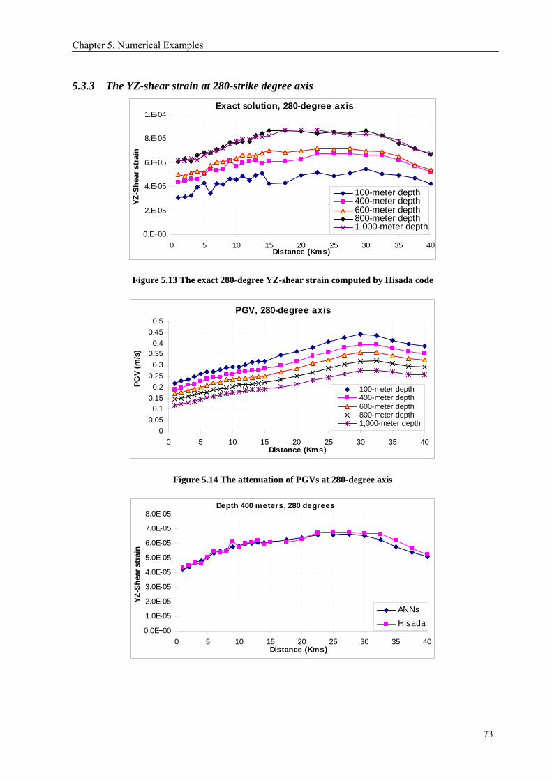
Chapter 5. Numerical Examples
5.3.3 The YZ-shear strain at 280-strike degree axis
Exact solution, 280-degree axis
0.E+00
2.E-05
4.E-05
6.E-05
8.E-05
1.E-04
0 5 10 15 20 25 30 35 40Distance (Kms)
YZ-S
hear
str
ain
100-meter depth400-meter depth600-meter depth800-meter depth1,000-meter depth
Figure 5.13 The exact 280-degree YZ-shear strain computed by Hisada code
PGV, 280-degree axis
00.050.1
0.150.2
0.250.3
0.350.4
0.450.5
0 5 10 15 20 25 30 35 40Distance (Kms)
PGV
(m/s
)
100-meter depth400-meter depth600-meter depth800-meter depth1,000-meter depth
Figure 5.14 The attenuation of PGVs at 280-degree axis
Depth 400 meters, 280 degrees
0.0E+00
1.0E-05
2.0E-05
3.0E-05
4.0E-05
5.0E-05
6.0E-05
7.0E-05
8.0E-05
0 5 10 15 20 25 30 35 40Distance (Kms)
YZ-S
hear
str
ain
ANNs
Hisada
73

Chapter 5. Numerical Examples
Depth 800 meters, 280 degrees
0.0E+001.0E-052.0E-053.0E-054.0E-055.0E-056.0E-057.0E-058.0E-059.0E-051.0E-04
0 5 10 15 20 25 30 35 40Distance (Kms)
YZ-S
hear
str
ain
ANNs
Hisada
Depth 1,000 meters, 280 degrees
0.0E+001.0E-052.0E-053.0E-054.0E-055.0E-056.0E-057.0E-058.0E-059.0E-051.0E-04
0 5 10 15 20 25 30 35 40Distance (Kms)
YZ-S
hear
str
ain
ANNs
Hisada
Figure 5.15 The comparison between 280-degree YZ-shear strain computed by Hisada and ANNs at
different depths
The ANNs’ and Hisada’s computation at 280-degree direction and at 400-meter depth provides a good agreement. However, the ANNs prediction accuracy is lower at deeper depth and at higher distance from the fault origin, caused by the effect of exceeding the upper bound of training data set in deeper depth. This effect can be seen as the requirement in choosing the appropriate observation point depth in the future and practical works. Moreover, the effect of PGV to the maximum shear strains can be seen clearly by the attenuation relationship of PGV and maximum shear strain in each direction.
74

Chapter 5. Numerical Examples
5.3.4 The YZ-shear strain at 315-strike degree axis
Exact solution, 315-degree axis
0.0E+00
1.0E-05
2.0E-05
3.0E-05
4.0E-05
5.0E-05
6.0E-05
0 5 10 15 20 25 30 35 40
Distance (Kms)
YZ-S
hear
str
ain
100-meter depth400-meter depth600-meter depth800-meter depth1,000-meter depth
Figure 5.16 The exact 315-degree YZ-shear strain computed by Hisada code
PGV, 315-degree axis
0
0.05
0.1
0.15
0.2
0.25
0 5 10 15 20 25 30 35 40Distance (Kms)
PGV
(m/s
)
100-meter depth400-meter depth600-meter depth800-meter depth1,000-meter depth
Figure 5.17 The attenuation of PGVs at 315-degree axis
Depth 100 meters, 315 degrees
0.0E+00
5.0E-06
1.0E-05
1.5E-05
2.0E-05
2.5E-05
3.0E-05
3.5E-05
0 5 10 15 20 25 30 35 40Distance (Kms)
YZ-S
hear
str
ain
ANNs
Hisada
75

Chapter 5. Numerical Examples
Depth 400 meters, 315 degrees
0.0E+00
5.0E-06
1.0E-05
1.5E-05
2.0E-052.5E-05
3.0E-05
3.5E-05
4.0E-05
4.5E-05
0 5 10 15 20 25 30 35 40Distance (Kms)
YZ-S
hear
str
ain
ANNs
Hisada
Depth 600 meters, 315 degrees
0.0E+005.0E-061.0E-051.5E-052.0E-052.5E-053.0E-053.5E-054.0E-054.5E-055.0E-05
0 5 10 15 20 25 30 35 40Distance (Kms)
YZ-S
hear
str
ain
ANNs
Hisada
Depth 800 meters, 315 degrees
0.0E+00
1.0E-05
2.0E-05
3.0E-05
4.0E-05
5.0E-05
6.0E-05
0 5 10 15 20 25 30 35 40Distance (Kms)
YZ-S
hear
str
ain
ANNs
Hisada
76

Chapter 5. Numerical Examples
Depth 1,000 meters, 315 degrees
0.0E+00
1.0E-05
2.0E-05
3.0E-05
4.0E-05
5.0E-05
6.0E-05
7.0E-05
0 5 10 15 20 25 30 35 40Distance (Kms)
YZ-S
hear
str
ain
ANNs
Hisada
Figure 5.18The comparison between 315-degree YZ-shear strain computed by Hisada and ANNs at
different depths
For 315-degree computation, which is completely different testing data from the training data set, the ANNs still can simulate the near-field YZ-shear strain at different depths. However, the ANNs’ computation at 315- degree YZ-shear strains and at 800- and 1,000-meter depth shows the limited of ANNs to predict the higher shear strain value than the ones that had been used as the training data. This effect can be seen as the requirement in choosing the appropriate observation points in the future and practical works. Moreover, the effect of PGV to the maximum shear strains can be seen clearly by the attenuation relationship of PGV and maximum shear strain in each direction.
5.3.5 The XY-shear strain at 0-strike degree axis
Exact solution, 0-degree axis
0.E+00
5.E-06
1.E-05
2.E-05
2.E-05
3.E-05
3.E-05
4.E-05
0 5 10 15 20 25 30 35 40Distance (meters)
XY -
Shea
r str
ain
100-meter depth400-meter depth600-meter depth800-meter depth1,000-meter depth
Figure 5.19 The exact 0-degree XY-shear strain computed by Hisada code
77

Chapter 5. Numerical Examples
PGV, 0-degree axis
00.020.040.060.080.1
0.120.140.160.180.2
0 5 10 15 20 25 30 35 40Distance (Kms)
PGV
(m/s
)
100-meter depth400-meter depth600-meter depth800-meter depth1000-meter depth
Figure 5.20 The attenuation of PGVs at 0-degree axis
Depth 400 meters, 0 degrees
0.0E+00
5.0E-06
1.0E-05
1.5E-05
2.0E-05
2.5E-05
3.0E-05
0 5 10 15 20 25 30 35 40Distance (Kms)
XY-S
hear
str
ain
ANNs
Hisada
Depth 800 meters, 0 degrees
0.0E+00
5.0E-06
1.0E-05
1.5E-05
2.0E-05
2.5E-05
0 5 10 15 20 25 30 35 40Distance (Kms)
XY-S
hear
str
ain
ANNs
Hisada
78

Chapter 5. Numerical Examples
Depth 1,000 meters, 0 degrees
0.0E+00
5.0E-06
1.0E-05
1.5E-05
2.0E-05
2.5E-05
0 5 10 15 20 25 30 35 40Distance (Kms)
XY-S
hear
str
ain
ANNs
Hisada
Figure 5.21 The comparison between 0-degree XY-shear strain computed by Hisada and ANNs at
different depths
The ANNs and Hisada’s computed shear strains show a good agreement, even at higher depth, i.e. 800- and 1,000-meter depth, since the training data sets provide the highest upper bound for shear strain in XY direction. Moreover, the effect of PGV to the maximum shear strains can be seen clearly by the attenuation relationship of PGV and maximum shear strain in each direction.
5.3.6 The XY-shear strain at 270-strike degree axis
Exact solution, 270-degree axis
0.0E+002.0E-054.0E-056.0E-058.0E-051.0E-041.2E-041.4E-041.6E-041.8E-04
0 5 10 15 20 25 30 35 40Distance (meters)
XY-S
hear
str
ain
100-meter depth400-meter depth600-meter depth800-meter depth1,000-meter depth
Figure 5.22 The exact 270-degree XY-shear strain computed by Hisada code
79

Chapter 5. Numerical Examples
PGV, 270-degree axis
0
0.1
0.2
0.3
0.4
0.5
0.6
0.7
0.8
0 5 10 15 20 25 30 35 40Distance (Kms)
PGV
(m/s
)
100-meter depth400-meter depth600-meter depth800-meter depth1000-meter depth
Figure 5.23 The attenuation of PGVs at 270-degree axis
Depth 400 meters, 270 degrees
0.0E+00
2.0E-05
4.0E-05
6.0E-05
8.0E-05
1.0E-04
1.2E-04
1.4E-04
1.6E-04
0 5 10 15 20 25 30 35 40Distance (Kms)
XY-S
hear
str
ain
ANNs
Hisada
Depth 800 meters, 270 degrees
0.0E+00
2.0E-05
4.0E-05
6.0E-05
8.0E-05
1.0E-04
1.2E-04
0 5 10 15 20 25 30 35 40Distance (Kms)
XY-S
hear
str
ain
ANNs
Hisada
80

Chapter 5. Numerical Examples
Depth 1,000 meters, 270 degrees
0.0E+001.0E-052.0E-053.0E-054.0E-055.0E-056.0E-057.0E-058.0E-059.0E-051.0E-04
0 5 10 15 20 25 30 35 40Distance (Kms)
XY-S
hear
str
ain
ANNs
Hisada
Figure 5.24 The comparison between 270-degree XY-shear strain computed by Hisada and ANNs at
different depths
It can be seen clearly that ANNs can learn and simulate the near-field XY-shear strain at different depths at 270-degree direction. The ANN’s computation provides a good result when the highest maximum shear strain had been chosen in the training data set. Moreover, the effect of PGV to the maximum shear strains can be seen clearly by the attenuation relationship of PGV and maximum shear strain in each direction.
5.3.7 The XY-shear strain at 280-strike degree axis
Exact solution, 280-degree axis
0.0E+001.0E-052.0E-053.0E-054.0E-055.0E-056.0E-057.0E-058.0E-059.0E-051.0E-04
0 5 10 15 20 25 30 35 40Distance (meters)
XY-S
hear
str
ain
100-meter depth400-meter depth600-meter depth800-meter depth1,000-meter depth
Figure 5.25 The exact 280-degree XY-shear strain computed by Hisada code
81

Chapter 5. Numerical Examples
PGV, 280-degree axis
00.050.1
0.150.2
0.250.3
0.350.4
0.450.5
0 5 10 15 20 25 30 35 40Distance (Kms)
PGV
(m/s
)
100-meter depth400-meter depth600-meter depth800-meter depth1,000-meter depth
Figure 5.26 The attenuation of PGVs at 280-degree axis
Depth 400 meters, 280 degrees
0.0E+00
1.0E-05
2.0E-05
3.0E-05
4.0E-05
5.0E-05
6.0E-05
7.0E-05
8.0E-05
9.0E-05
0 5 10 15 20 25 30 35 40Distance (Kms)
XY-S
hear
str
ain
ANNs
Hisada
Depth 800 meters, 280 degrees
0.0E+00
1.0E-05
2.0E-05
3.0E-05
4.0E-05
5.0E-05
6.0E-05
7.0E-05
0 5 10 15 20 25 30 35 40Distance (Kms)
XY-S
hear
str
ain
ANNs
Hisada
82
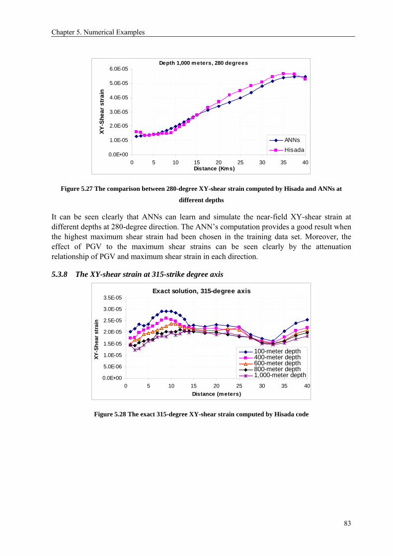
Chapter 5. Numerical Examples
Depth 1,000 meters, 280 degrees
0.0E+00
1.0E-05
2.0E-05
3.0E-05
4.0E-05
5.0E-05
6.0E-05
0 5 10 15 20 25 30 35 40Distance (Kms)
XY-S
hear
str
ain
ANNs
Hisada
Figure 5.27 The comparison between 280-degree XY-shear strain computed by Hisada and ANNs at
different depths
It can be seen clearly that ANNs can learn and simulate the near-field XY-shear strain at different depths at 280-degree direction. The ANN’s computation provides a good result when the highest maximum shear strain had been chosen in the training data set. Moreover, the effect of PGV to the maximum shear strains can be seen clearly by the attenuation relationship of PGV and maximum shear strain in each direction.
5.3.8 The XY-shear strain at 315-strike degree axis
Exact solution, 315-degree axis
0.0E+00
5.0E-06
1.0E-05
1.5E-05
2.0E-05
2.5E-05
3.0E-05
3.5E-05
0 5 10 15 20 25 30 35 40Distance (meters)
XY-S
hear
str
ain
100-meter depth400-meter depth600-meter depth800-meter depth1,000-meter depth
Figure 5.28 The exact 315-degree XY-shear strain computed by Hisada code
83

Chapter 5. Numerical Examples
PGV, 315-degree axis
0
0.05
0.1
0.15
0.2
0.25
0 5 10 15 20 25 30 35 40Distance (Kms)
PGV
(m/s
)
100-meter depth400-meter depth600-meter depth800-meter depth1,000-meter depth
Figure 5.29 The attenuation of PGVs at 315-degree axis
Depth 100 meters, 315 degrees
0.0E+00
5.0E-06
1.0E-05
1.5E-05
2.0E-05
2.5E-05
3.0E-05
3.5E-05
4.0E-05
0 5 10 15 20 25 30 35 40Distance (Kms)
XY-S
hear
str
ain
ANNs
Hisada
Depth 400 meters, 315 degrees
0.0E+00
5.0E-06
1.0E-05
1.5E-05
2.0E-05
2.5E-05
3.0E-05
3.5E-05
0 5 10 15 20 25 30 35 40Distance (Kms)
XY-S
hear
str
ain
ANNs
Hisada
84

Chapter 5. Numerical Examples
Depth 600 meters, 315 degrees
0.0E+00
5.0E-06
1.0E-05
1.5E-05
2.0E-05
2.5E-05
3.0E-05
0 5 10 15 20 25 30 35 40Distance (Kms)
XY-S
hear
str
ain
ANNs
Hisada
Depth 800 meters, 315 degrees
0.0E+00
5.0E-06
1.0E-05
1.5E-05
2.0E-05
2.5E-05
3.0E-05
0 5 10 15 20 25 30 35 40Distance (Kms)
XY-S
hear
str
ain
ANNs
Hisada
Depth 1,000 meters, 315 degrees
0.0E+00
5.0E-06
1.0E-05
1.5E-05
2.0E-05
2.5E-05
0 5 10 15 20 25 30 35 40Distance (Kms)
XY-S
hear
str
ain
ANNs
Hisada
Figure 5.30 The comparison between 315-degree XY-shear strain computed by Hisada and ANNs at
different depths
For 315-degree computation, which is completely different testing data from the training data set, the ANNs still can learn and simulate the near-field YZ-shear strain at different depths.
85

Chapter 6: Conclusion and Future Research
6 CONCLUSION AND FUTURE RESEARCH
6.1 Introduction Since the effects of near fault effect owned to the forward directivity and fling step effects contribute to the underground structural damages, which are largely different from that in the far-field case. Corigliano, M., et al. [2007] developed the pseudo-static equations to predict the seismic stress increment in the lining. The comparison between the pseudo-static and numerical examples showed a reasonable result from his study. From the equation (3.44) and (3.45), the seismic forces can be predicted correctly from the prediction of the maximum shear strain that is the key parameter and it is the main concern in this study. The simplified tool, the ANNs, had been developed and calibrated to compute the maximum shear strain under free-field in near-fault region.
To develop an ANNs-based method to determine the maximum shear strain, the “Ariano Irpino” fault in the “Sannio” region had been used as the seismic source in this study which its near-fault ground motion record was generated by semi analytical method developed by Hisada and Bielak [2003]. To compute the earthquake-induced shear strain field in the vicinity of a causative fault, the displacement at six points around the interested observation points is calculated, and the shear strains can be calculated based on equation (5.1).
Since the ANNs need training data set in order to learn the near-field ground motion characteristics, the 100- and 600- meter depth and at 0-, 270-, and 280- strike degree data set had been used for this purpose. The trained ANNs would then be tested to predict the maximum shear strain at 400-, 800-, and 1,000-meter depth and at 0-, 270-, 280-, and 315- strike degree).
6.2 Numerical examples The choosing of observation points as a training data set is very important, since the ANNs is highly affected to the quality of training data set. From Figure 5.12, in 270 degrees at 800- and 1,000- meter depths, the computed maximum YZ-shear strain are clearly over predict the target result. The main reason is the training data set, 100- and 600-meter depths have lower maximum shear strain ordinate than that at800- and 1,000-meter depths. This observation should be considered for installation of the seismograms or accelerometers in order to improve the ANNs’ computation accuracy.
From the numerical calculation, the ANNs can predict the maximum shear strain in the same
86

Chapter 6: Conclusion and Future Research
direction as using in training data set but at different depth, with a reasonable accuracy as long as the limit of upper bound of training data set does not exceed, Figure 5.9, 5.21, 5.24.
The computed result from ANNs in different strike angles and depths from the training data set give a rationally acceptable as long as the limit of upper bound of training data set does not exceed, Figure 5.30.
6.3 Future research From this study, the prediction of the earthquake-induced maximum shear strain in the ground under free-field condition had been proposed. The numerical examples show a possible capability of ANNs in computing the maximum shear strains around the studied fault.
The applicable of ANNs to determine the maximum free-field shear strain should be applied to other fault geometries and earthquake magnitudes to test the versatility of ANNs. Moreover, the choosing of observation points in order to optimize and increase the predicted accuracy should be also investigated.
87

References
REFERENCES
AASHTO [1998] LRFD Bridge Design Specifications, Second Edition, 2001 Interim Revisions, American Association of State Highway and Transportation Officials, Washington DC.
AKI, K. [1993]. “Local site effects on weak and strong ground motion,” Tectonophysics, 218, pp. 93-111.
American Lifelines Alliance [2001], Seismic Fragility Formulations for Water Systems.
Asakura T and Sato Y, [1998] “Mountain Tunnels Damage in the 1995 HYOGOKEN-NANBU Earthquake,” QR of Railway Technical Research Institute (RTRI), 39(1) pp. 9–16.
Bommer, J.J. & Martinez-Pereira, A. [1999]. “The effective duration of earthquake strong motion,” Journal of Earthquake Engineering, 3 (2), pp. 127-172.
Bray and Rodriguez-Marek [2004] “Characterization of forward directivity ground motion in the near fault region.” Soil Dynamic and Earthquake Engineering, 24, pp. 815-828.
Burns, J. Q., and Richard, R. M. [1964] “Attenuation of stresses for buried cylinders,” Proceeding of the Symposium on Soil-Structure Interaction, University of Arizona at Tempe, Arizona.
Hoeg, K. [1968] “Stresses against underground structural cylinders,” Journal Soil Mechanics Found. Div., ASCE 94 (SM4), pp. 883-858.
Corigliano, M., Scandella, L., Barla, G., Lai, C. G., Paolucci, R. [2007] “Seismic analysis of deep tunnels in weak rock: a case study in southern Italy,” Procceding of 4th International Conference on Earthquake Geotechnical Engineering, Paper No. 1616, Thessaloniki, Greece
Cotecchia V, [1986] “Ground deformations and slope instability produced by the earthquake of 23 November 1980 in Campania and Basilicata,” International symposium on Engineering Geology in Seismic Areas. Bari, Italy: Institution of Engineering Geology and Geotechnics, University of Bari, Italy.
Cotton, F., Scherbaum, F., Bommer, J. J., and Bungum, H. [2006] “Criteria for selecting and adjusting ground motion models for specific target regions: Application to Central Europe and rock sites,“ Journal of Seismology, 10, pp.137-156
DISS v. 3.0.1 [2006]: Database of Individual Seismogenic Sources: A compilation of potential sources for earthquakes larger than M 5.5 in Italy and surrounding areas. http://www.ingv.it/DISS/.
Dowding, C.H., Rozen, A. [1978] “Damage to Rock Tunnels from Earthquake Shaking,” Journal of
88

References
Geotechnical Engineering Division, ASCE 104 GT2, pp. 175- 191
Einstein H. H. and Schwartz C. W. [1979] “Simplified analysis for tunnel support,“ Journal of the geotechnical engineering division, 105, pp. 499-518.
Japanese Society of Civil Engineers, JSCE [1975] Specification for Earthquake Resistant Design of Submerged Tunnels.
Jenning, P. C. [1985] “Ground motion parameters that influence structural damage,” in R.E. Scholl and J.L. King, eds. Strong Ground Motion Simulation and Engineering Applications, EERI Publication 85-02, EERI, Berkeley, 298 pp.
Joyner, W.B. and Boore, D.M. [1988] “Measurement, characterization, and prediction of strong ground motion,” in Earthquake Engineering and Soil Dynamics II – Recent Advances in Ground Motion Evaluation, Geotechnical Special Publication 20, ASCE, New York, pp. 43-102.
Gomez-Masso, A. and Attalla, I. [1984] “Finite element vs. simplified methods in the seismic analysis of underground structures,” Earthquake Engineering and Structural Dynamics, 12, pp. 347-367.
Hashash, M. A. Youssef, Hook, J., Jeffrey, Schmidt Birger, Yao, John I-Chiang [2001] “Seismic design and analysis of underground structures,” Tunneling and Underground Space Technology Vol. 16, pp. 247-293.
Hashash. Y.M.A., Tseng, W.S. and Krimotat, A. [1998] “Seismic Soil-structure Interaction Analysis for Immersed Tube Tunnels Retrofit,” Geotechnical Earthquake Engineering and Soil Mechanics. Vol. I11 2, pp. 1380-1391. ASCE Geotechnical Special Publication no. 75.
Haykin, S. [1998] Neural Networks: A Comprehensive Foundation. Prentice Hall, 2nd edition.
Hertz, J., Krogh, A., and Palmer, R. G. [1991], “An Introduction to the Theory of Neural Computation”. Lecture Notes, Volume I. Addison-Wesley, Redwood City, CA.
Hisada Y. and Bielak J., [2003] “A theoretical method for computing near fault ground motion in a layered half-spaces considering static offset due to surface faulting, with a physical interpretation of fling step and rupture directivity,” Bulletin of the Seismological Society of America 93(3), pp. 1154-1168.
Hwang, R.N., and Lysmer, J. [1981] “Response of Buried Structures to Traveling Waves,” Journal of the Geotechnical Engineering Division, ASCE, Vol. 107, No. GT2.
Idriss, I.M. and Seed, H.B. [1968] “Seismic response of horizontal soil layers,” J. Soil mech. Found. Div., ASCE 94 (SM4), pp. 1003-1031.
Improta, L., Iannaccone, G., Capuano P., Zollo, A., Scandone, P., [2000] “Inferences on the upper crustal structure of Southern Apennines (Italy) from seismic refraction investigations and subsurface data,” Tectonophysics, 317, pp. 273-297.
Indrawan, B., [2001] “Lessons learned from past Earthquake Damages and seismic Observation of Tunnel Structures,” Tunneling seminar, University of Pelita Harapan. Karawachi, Indonesia.
Kawashima, K. [2000] “Seismic Design of Underground Structures in Soft Soil Ground: A Review, Key Note Presentation,” Geothechnical Aspects of Underground Construction in Soft Ground, Balkema, Rotterdam, 3-19, 2000
Kramar, S. L. [1996]. Geotechnical Earthquake Engineering. New Jersey: Prentice Hall.
89

References
Kuesel, T.R. [1969]. “Earthquake Design Criteria for Subways,” Journal of Structure Division, ASCE ST6, pp. 1213- 1231.
McGarr, A. [1983]. “Estimated ground motion for small near-by earthquakes,” Seismic Design of Embankment and Caverns, pp. 113-127. New York: ASCE.
Monsees, J.E. and Merritt J.L., [1988] “Seismic modeling and design of underground structures,” Numerical Methods in Geomechanics, Innsbruck, pp. 1833-1842.
Monsees, J.E. and Merritt J.L., [1991] “Earthquake considerations in design of the Los Angeles Metro,” Proceeding of the ASCE Conference on Lifeline Earthquake Engineering.
Newmark, N. M. [1967] “Problems in wave propagation in soil and rocks,” Proceedings of the International Symposium on Wave Propagation and Dynamic Properties of Earth Materials, University of New Mexico Press, pp.7-26.
Okamoto, S. [1973], Introduction to Earthquake Engineering, University of Tokyo Press, Tokyo, Japan, 1973.
Owen, G.N. and Scholl, R.E. [1981] Earthquake Engineering of Large Underground Structures. Report no. FHWARD-80-195, Federal Highway Administration and National Science Foundation.
Peck , R.B., Hendron, A.J., Mohraz, B.,[1972] “State of the art in soft ground tunneling,” Proceeding of the Rapid Excavation and Tunneling Conference. American Institute of Mining, Metallurgical and Petroleum Engineers, New York, pp. 259-286.
Power, M.S., Rosidi, D., and Kaneshiro, J., [1996], Vol. III Strawman: screening, evaluation, and retrofit design of tunnels, Report Draft National Center for Earthquake Engineering Research, Buffalo, New York.
Power, M.S., Rosidi, D., and Kaneshiro, J., Gilstrap, S.D., and Chiou, S.J. [1998], “Summary and Evaluation of Procedures for the Seismic Design of Tunnels: Multidisciplinary Center for Earthquake Engineering Research,” Draft Technical Report, FHWA Contract No. DTFH61-92-C-0012 Task 112-D-5.3c, Sept. 1998.
Richardson, A., and Blejwas T. E. [1992] “Seismic Design of Circular-Section Concrete-Lined Underground Openings — Preclosure Performance Considerations for the Yucca Mountain Site,” ASCE Symposium on Dynamic Analysis and Design Considerations for High-Level Nuclear Waste Repositories.
Rumelhart, D. E., Hinton, G. E., and Williams, R. J. [1986] “ A Learning representations by back-propagating errors,” Nature 323: pp. 533-536.
Sanner, R.M. and Slotine, J-J.E. [1992] “Gaussian networks for direct adaptive control,” IEEE Transcations on Neural Network 2(6):pp. 837-863.
Sakurai, A. and Takahashi, T. [1969] “Dynamic stresses of underground pipeline during earthquakes,” Proceeding of the Fourth World Conference on Earthquake Engineering.
Tzirkel-Hancock, E. and Fallside, F. [1992] “Stable control of nonlinear systems using neural networks,” International Journal of Robust and Nonlinear Control, 2(1): pp. 63-86.
Sharma S and Judd W R, [1991] “Underground opening damage from earthquakes,” Engineering Geology, Vol. 30: pp. 263–276.
90

References
Simpson, K.A. [1996]. “Attenuation of strong ground-motion incorporating near-surface foundation conditions.” Doctoral Thesis, University of London.
Somerville, P.G., Smith, N.F., Graves, R.W., and Abrahamson, N.A. [1997] “Modification of empirical strong ground motion attenuation relationships to include the amplitude and duration effects of rupture directivity,” Seismological Research Letters, 68 (1), pp.199-222.
SOMERVILLE, P. [1998] “Ground motion attenuation relationships and their application to aseismic design and seismic zonation,” In: Irikura, Kudo, Okada & Sasatani (eds) The effects of Surface Geology on Seismic Motion. pp.35-49.
Somerville, P. [2000] “Characterization of Near-Fault Ground Motions,” Proceeding of the U.S.-Japan Workshop on the Effects of Near-Field Earthquake Shaking, Pacific Earthquake Engineering Research Center, pp. 21-30.
St. John, C.M. and Zahrah, T.F. [1987] “Aseismic Design of Underground Structures,” Tunneling Underground Space Technology. Vol. 22, pp. 165 - 197.
Stewart, J. P., Chiou, S. J., Bray, J. D., Graves, R. W., Somerville, P. G., Abrahamson, N. A., [2001], “Ground Motion Evaluation Procedures for Performance-Based Design”, Report PEER 2001/09.
Sweet, J. [1997] “Los Angeles Metro Red Line project: seismic analysis of the Little Tokyo Subway Station,” Report no. CAI-097-100. Engineering Management Consultants.
Tso, W.K., Zhu, T.J. & Heidebrecht, A.C. [1992] “Engineering implication of ground motion A/V ratio,” Soil Dynamics and Earthquake Engineering. 11, pp.133-144.
Yoshikawa, K., Fukuchi, G. [1984] “Earthquake Damage to Railway Tunnels in Japan,” Advances in Tunneling Technology and Subsurface Use, Vol.4 Nr.3, pp. 75-83
W.L. Wang, T.T. Wang, J.J. Su, C.H. Lin, C.R.Seng, T.H.Huang, [2001] “Assessment of damage in
mountain tunnels due to the Taiwan Chi-Chi Earthquake,” Tunneling and Underground Space
Technology, Vol 16, pp. 133-150
Wang, J. N. [1993] “Seismic Design of Tunnels, A State-of-the-Art Approach,” Monograph 7, Parsons Brickerhoff Quade & Douglas, Inc., New York.
Zurada, J. M. [1992], Artificial Neural Systems. West Publishing Company, St. Paul, MN.
91