annex 2 step-by-step guideline for mike 11-rr …open_jicareport.jica.go.jp/pdf/174438_03.pdf ·...
TRANSCRIPT
1
Annex 2
Step-by-step Guideline
for
MIKE 11-RR (NAM) Model
Biala River basin (EABD)
Pirinska Bistritsa River basin (WABD)
JICA Study Team

2

3
1. Biala River Basin
62800
HMS
Catchment_HMS62800
RiverNetworkMIKE11
MainRiverSegment
NAMCatchment
Catchment
/ Available information for model
From Core Data of GIS-DB
- Digital elevation model (50m grid)
- RiverNetwork and Catchment boundary
From Analysis Data of GIS-DB
- Monthly Potential Evapo-Transpiration (1km grid)
From TimeSeries Data of GIS-DB
- Daily average water quantity at HMS 62800 (2000 – 2005)
- Daily precipitation at precipitation sts. at 43450, 44410, 44420 (2000 –
2005)
- Daily average temperature at Meteorological st. at 43010 (Haskovo) (2000-
2005)
-
/ Model setting
Total catchment Area: 598.77 km2
Number of catchment for Rainfall-Runoff model (NAM Catchment): 1
Number of river for MIKE11-HD: 1 (for next exercise)
In this exercise, effect of water abstraction and waste water discharge is neglected.
Therefore, it is regarded that daily average water quantity at 62800 is almost equal to
quasi-natural water quantity.

4
(1) Input data
1) Average Precipitaton
62800
43450
4441044420
Thiessen Polygon
Precipitation St.
HMS
Catchment_HMS62800
RiverNetworkMIKE11
NAMCatchment
Average precipitation over a catchment is estimated by the following equation.
0aveelcave PCP =
( )[ ]P_aveaveele EE.expC -00030=
npnave PCP 0 =
npnp_ave ECE =
where Pave = average precipitation (mm), Pave0 = average precipitation before
correction for elevation difference (mm), Cele = correction coefficient for
elevation difference between average elevation of catchment and one for
precipitation sts. (-), Eave = average elevation of catchment (m), Eave_p = average
elevation of precipitation stations (m), Pn = precipitation at station “n” (mm), Cpn
= Thiessen coefficient for station “n” (-), En = elevation at station “n” (m).
Average elevation of catchment is derived from digital elevation model.

5
Thiessen coefficients for each precipitation station are calculated as follows.
Total catchment of Biala River Basin (NAM Catchment: BI_M)
Average elevation of catchment (m)
Eave
418Catchment Area
(km2)
598.77
Station No. 43450 44410 44420 Average elevation of
Precipitation sts. Eave_P
Thiessen Coefficient Cpn
0.060 0.643 0.296 N/A
Elevation (m) En
240 100 450 212
Correction coefficient for elevation difference (m)
Cele
1.064
Watershed for HMS62800
Average elevation of catchment (m)
Eave
452CatchmentArea (km
2)
506.71
Station No. 43450 44410 44420 Average in catchment
Eave_P
Thiessen Coefficient Cpn
0.071 0.579 0.350 N/A
Elevation (m) En
240 100 450 233
Correction coefficient for elevation difference (m)
Cele
1.068
2) Average Potential Evapo-Transpiration
Average potential evapo-transpiration for a catchment is derived from 1km grid
monthly evapo-transpiration.
3) Daily Average Temperature
Daily average temperature at Meteorological st. at 43010 (Haskovo) is directly
used for simulation.
Elevation of Meteorological St. (m) at 43010
230

6
4) Elevation zone distribution
Catchment area is divided into several elevation zones for snow module in
NAM model. Based on digital elevation model, area for each elevation zone
within total catchment area is calculated as follows.
Total Catchment of Biala River Basin (NAM Catchment: BI_M)
Elevation Zone (m)
0 – 200 200 - 400 400 -600 600 - 800800 - 1000
1000- 1200
1200- 1400
Representative Elevation (m)
100 300 500 700 900 1100 1300
Area (km2) 59.58 231.92 210.33 77.28 13.32 6.26 0.08
Elevation Zone (m)
1400- 1600
1600- 1800
1800- 2000
2000- 2200
2200- 2400
2400- 2600
2600- 2800
Representative Elevation (m)
1500 1700 1900 2100 2300 2500 2700
Area (km2) 0.00 0.00 0.00 0.00 0.00 0.00 0.00
Watershed for HMS62800
Elevation Zone (m)
0 – 200 200 - 400 400 -600 600 - 800800 - 1000
1000- 1200
1200- 1400
Representative Elevation (m)
100 300 500 700 900 1100 1300
Area (km2) 21.57 183.45 204.76 77.28 13.32 6.26 0.08
Elevation Zone (m)
1400- 1600
1600- 1800
1800- 2000
2000- 2200
2200- 2400
2400- 2600
2600- 2800
Representative Elevation (m)
1500 1700 1900 2100 2300 2500 2700
Area (km2) 0.00 0.00 0.00 0.00 0.00 0.00 0.00
5) Precipitation correction for each elevation zone
Catchment area is divided into several elevation zones for snow module in
NAM model. Amount of precipitation for each elevation zone is corrected
based on the following equation.
( )[ ]{ }1-00030100 aveii EE.expR =
where Ri = Correction ratio (%), Ei = average elevation of each elevation zone
(m), Eave = average elevation of catchment (m),.
Correction ratio for each elevation zone is calculated as follows.

7
Total Catchment of Biala River Basin (NAM Catchment: BI_M)
Elevation Zone (m)
0 – 200 200 - 400 400 -600 600 - 800800 - 1000
1000- 1200
1200- 1400
Representative Elevation (m)
100 300 500 700 900 1100 1300
Ri (%) -9.09 -3.47 2.50 8.83 15.56 22.71 30.30
Elevation Zone (m)
1400- 1600
1600- 1800
1800- 2000
2000- 2200
2200- 2400
2400- 2600
2600- 2800
Representative Elevation (m)
1500 1700 1900 2100 2300 2500 2700
Ri (%) 38.35 46.91 55.99 65.64 75.88 86.76 98.31
Watershed for HMS62800
Elevation Zone (m)
0 – 200 200 - 400 400 -600 600 - 800800 - 1000
1000- 1200
1200- 1400
Representative Elevation (m)
100 300 500 700 900 1100 1300
Ri (%) -10.02 -4.46 1.45 7.72 14.39 21.46 28.97
Elevation Zone (m)
1400- 1600
1600- 1800
1800- 2000
2000- 2200
2200- 2400
2400- 2600
2600- 2800
Representative Elevation (m)
1500 1700 1900 2100 2300 2500 2700
Ri (%) 36.94 45.41 54.40 63.95 74.09 84.85 96.29
6) Input file name
Total catchment of Biala River
Basin (NAM Catchment: BI_M)
Watershed for HMS62800
DailyPrecipitation DailyPrecipitation_Biala.dfs0 DailyPrecipitation_62800.dfs0
Monthly PET MonthlyPET_Biala.dfs0 MonthlyPET_62800.dfs0
DailyAveTemperature DailyAveTemperature.dfs0 DailyAveTemperature.dfs0
DailyAveWaterQuantity
for calibration
N/A DailyAveDischarge_62800.dfs0
Elevation zone NAM_Parameters_Training.xls NAM_Parameters_Training.xls
Precipitation correction
ratio for each elevation
zone
NAM_Parameters_Training.xls NAM_Parameters_Training.xls

8
2. Pirinska Bistritsa River Basin
51590
HMS
Catchment_HMS51590
RiverNetworkMIKE11
MainRiverSegment
NAMCatchment
Catchment
/ Available information for model
From Core Data of GIS-DB
- Digital elevation model (50m grid)
- RiverNetwork and Catchment boundary
From Analysis Data of GIS-DB
- Monthly Potential Evapo-Transpiration (1km grid)
From TimeSeries Data of GIS-DB
- Daily average water quantity at HMS 51590 (2000 – 2005)
- Daily precipitation at precipitation sts. at 61600, 61610, 61640, 61660,
61670 (2000 – 2005)
- Daily average temperature at Meteorological st. at 15712 (Sandanski)
(2000- 2005)
/ Model setting
Total catchment Area: 508.29 km2
Number of catchment for Rainfall-Runoff model (NAM Catchment): 1
Number of river for MIKE11-HD: 1 (for next exercise)
In this exercise, effect of water abstraction and waste water discharge except
intake by Pirinska Bistritsa-HPP is neglected. Observed data at HMS51590 is
strongly affected by HPP. Based on monthly used water amount by Pirinska
Bistritsa HPP, quasi-natural flow at HMS 51590 is estimated (2001-2004 only).

9
(2) Input data
1) Average Precipitaton
51590
61600
61610
61640
61660
61670
Thiessen Polygon
Precipitation St.
HMS
Catchment_HMS51590
RiverNetworkMIKE11
NAMCatchment
Average precipitation over a catchment is estimated by the following equation.
0aveelcave PCP =
( )[ ]P_aveaveele EE.expC -00030=
npnave PCP 0 =
npnp_ave ECE =
where Pave = average precipitation (mm), Pave0 = average precipitation before
correction for elevation difference (mm), Cele = correction coefficient for
elevation difference between average elevation of catchment and one for
precipitation sts. (-), Eave = average elevation of catchment (m), Eave_p = average
elevation of precipitation stations (m), Pn = precipitation at station “n” (mm), Cpn
= Thiessen coefficient for station “n” (-), En = elevation at station “n” (m).
Average elevation of catchment is derived from digital elevation model.

10
Thiessen coefficients for each precipitation station are calculated as follows.
Total catchment of Pirinska Bistritsa River Basin (NAM Catchment: ST_PIR)
Average elevation of catchment (m)
Eave
1015 CatchmentArea (km
2)
508.29
Station No. 61600 61610 61640 61660 61670 Average elevation of
Precipitation sts. Eave_P
Thiessen Coefficient Cpn
0.100 0.377 0.059 0.167 0.298 N/A
Elevation (m) En
710 760 100 860 382 620
Correction coefficient for elevation difference (m)
Cele
1.126
Watershed for HMS51590
Average elevation of catchment (m)
Eave
1507 CatchmentArea (km
2)
133.71
Station No. 61600 61610 61640 61660 61670 Average elevation of
Precipitation sts. Eave_P
Thiessen Coefficient Cpn
0.012 0.047 0.00 0.624 0.318 N/A
Elevation (m) En
710 760 100 860 382 702
Correction coefficient for elevation difference (m)
Cele
1.273
2) Average Potential Evapo-Transpiration
Average potential evapo-transpiration for a catchment is derived from 1km grid
monthly evapo-transpiration.
3) Daily Average Temperature
Daily average temperature at Meteorological st. at 15712 (Sandanski) is
directly used for simulation.
Elevation of Meteorological St. (m) at 15712
206

11
4) Elevation zone distribution
Catchment area is divided into several elevation zones for snow module in
NAM model. Based on digital elevation model, area for each elevation zone
within total catchment area is calculated as follows.
Total Catchment of Pirinska Bistritsa River Basin (NAM Catchment: ST_PIR)
Elevation Zone (m)
0 – 200 200 - 400 400 -600 600 - 800800 - 1000
1000- 1200
1200- 1400
Representative Elevation (m)
100 300 500 700 900 1100 1300
Area (km2) 18.39 62.09 70.96 51.35 58.09 52.20 60.76
Elevation Zone (m)
1400- 1600
1600- 1800
1800- 2000
2000- 2200
2200- 2400
2400- 2600
2600- 2800
Representative Elevation (m)
1500 1700 1900 2100 2300 2500 2700
Area (km2) 51.65 34.10 20.09 11.41 10.10 7.10 0.00
Watershed for HMS51590
Elevation Zone (m)
0 – 200 200 - 400 400 -600 600 - 800800 - 1000
1000- 1200
1200- 1400
Representative Elevation (m)
100 300 500 700 900 1100 1300
Area (km2) 0.00 0.18 3.22 7.98 10.92 14.62 22.06
Elevation Zone (m)
1400- 1600
1600- 1800
1800- 2000
2000- 2200
2200- 2400
2400- 2600
2600- 2800
Representative Elevation (m)
1500 1700 1900 2100 2300 2500 2700
Area (km2) 18.49 18.15 12.56 8.34 10.09 7.10 0.00
5) Precipitation correction for each elevation zone
Catchment area is divided into several elevation zones for snow module in
NAM model. Amount of precipitation for each elevation zone is corrected
based on the following equation.
( )[ ]{ }1-00030100 aveii EE.expR =
where Ri = Correction ratio (%), Ei = average elevation of each elevation zone
(m), Eave = average elevation of catchment (m),.
Correction ratio for each elevation zone is calculated as follows.

12
Total Catchment of Pirinska Bistritsa River Basin (NAM Catchment: ST_PIR)
Elevation Zone (m)
0 – 200 200 - 400 400 -600 600 - 800800 - 1000
1000- 1200
1200- 1400
Representative Elevation (m)
100 300 500 700 900 1100 1300
Ri (%) -24.02 -19.32 -14.33 -9.03 -3.40 2.57 8.91
Elevation Zone (m)
1400- 1600
1600- 1800
1800- 2000
2000- 2200
2200- 2400
2400- 2600
2600- 2800
Representative Elevation (m)
1500 1700 1900 2100 2300 2500 2700
Ri (%) 15.65 22.80 30.39 38.45 47.01 56.11 65.76
Watershed for HMS51590
Elevation Zone (m)
0 – 200 200 - 400 400 -600 600 - 800800 - 1000
1000- 1200
1200- 1400
Representative Elevation (m)
100 300 500 700 900 1100 1300
Ri (%) -34.43 -30.38 -26.07 -21.50 -16.65 -11.49 -6.02
Elevation Zone (m)
1400- 1600
1600- 1800
1800- 2000
2000- 2200
2200- 2400
2400- 2600
2600- 2800
Representative Elevation (m)
1500 1700 1900 2100 2300 2500 2700
Ri (%) -0.21 5.96 12.51 19.47 26.86 34.70 43.03
6) Input file name
Total catchment of Pirinska
Bistritsa River Basin
(NAM Catchment: ST_PIR)
Watershed for HMS51590
DailyPrecipitation DailyPrecipitation_PirinskaB.dfs0 DailyPrecipitation_51590.dfs0
Monthly PET MonthlyPET_PirinskaB.dfs0 MonthlyPET_51590.dfs0
DailyAveTemperature DailyAveTemperature.dfs0 DailyAveTemperature.dfs0
DailyAveWaterQuantity
for calibration
N/A DailyAveDischarge_51590_cal.dfs0
Area for each elevation
zone
NAM_Parameters_Training.xls NAM_Parameters_Training.xls
Precipitation correction
ratio for each elevation
zone
NAM_Parameters_Training.xls NAM_Parameters_Training.xls

13
3. Model set-up
Here, example for Biala River Basin is shown. Set-up procedure for Pirinska
Bistritsa River Basin is principally same.

14
Copy the folder”MIKE11_Training”
from CD, which includes training
material, to hard disk in your
computer.
Start MIKE11 from “start menu”.
Now, MIKE11 with MIKE ZERO
platform started.

15
Setting Option in MIKE
Zero
Select File -> Options -> User
Setting
Set Default Project Folder, (if
necessary).
Check “Enable Dynamic Show
all”.
(Important!)
Click “OK”.
Restart MIKE11
Making a new project
File -> New -> Project from
Folders

16
Dialog “New Project from Folder”
appears.
Browse the folder”MIKE11_Training”
which was copied to the hard disk in
your computer.
Enter Project Name.
Then, click “Next (N)”.
Make sure all are checked in check
boxes.
Then click “complete”.

17
New project opened.
Once a new project is set, from next
time, you can open the project by
clicking Name of project shown in
“Open an Existing Project”.
Right click “MIKE11_Traing” folder.
Click “Show all”.
(Important!)
Without doing this, newly added files
in the project are not visible.

18
Setting-up rainfall-runoff
model for calibration
In Project Explorer, place cursor on
“Biala_Cal”, then right click.
Select “Add Folder”.
Dialog “New Folder” appears.
Input folder name. Then, click “OK”.
New folder “62800” under
“Biala_Cal” is now in Project
Explorer.

19
In Project Explorer, place cursor on
“62800”, then right click.
Select “Add New File”.
Dialog “New Folder” appears.
Select
MIKE11 -> RR Parameters(RR11)
Then. Click “OK”

20
Dialog “RRPar1” appears.
Click ”Insert catctment”
Set the name for “Catchment name”
Select “NAM” from Rainfall runoff
model.
Set the value for “ Catchment area”.
Then, click “OK”.
Now, a catchment is set.
You can see the inserted catchment
in “Catchment Overview”.

21
Check “Calibration plot”.
By checking this, you can get
“calibration plot”, which shows
observed and simulated hydrograph
together, when you conduct a
simulation run.
Select” NAM” tab.
You can see that default parameters
are already set in
“Surface-Rootzone” tab.
Keep default values.
(Later, auto-calibration will be done.)
Select” GroundWater” tab.
Check “Lower baseflow….”.
Set the value for “Cqlow”, “Cklow”.
Note:
There is an option not to use
“LowerGroundWater component”.
However, the study results show that
to include “LowerGroundWater
component” gives better results for
recession process.

22
Select” SnowMelt” tab.
Check “Include snow melt”.
Set values for “Csnow”,”T0”.
Check “Delineation of catchment into
elevation zone”.
Click “Edit Zones”.
Dialog “Elevation Zones” appears.
Set values ”Number of elevation
zone”, Reference level for
temperature station”
Click “OK”.

23
Form folder for training material,
open ./003_XLS/NAM_Paramaters_T
raining.xls”.
Activate sheet
“ElevationZone_Adjusted”/
Copy elevation zone.
Open again dialog “Elevation Zones”.
Click “elevation”. Then, paste the
copied from.xls file.
Repeat same procedure for “Area”,
“Correction of precipitation”.

24
Set values for “Min storage for full
coverage” to 100 (default value) for
all elevation zones.
Set values for “Max storage in
zone” to 10000 (default value) for all
elevation zones.
Set values for “Maximum water
retained in snow”.
Based on the calibration results for
EABD&WABD catchments, the
followings are the most
recommended values.
Zone:100-1300 -> 0
Zone:1500 -> 50
Zone: 1500- 2700 -> 100
Check “Dry temperature lapse rate”,
“Wet temperature lapse rate”.
Set values for Dry temperature
lapse rate”, “Wet temperature lapse
rate”. (Default values are -0.6 and
-0.4, respectively.)
Click “Calculate”. Then the
correction values of temperature for
each elevation zone are
automatically assigned.
Finally, click “OK”.

25
Select” Irrigation” tab.
Make sure that”Include irrigation” is
not checked.
Select” Initial Condition” tab.
Set values for initial conditions.
Please refer
“./003_XLS/NAM_Paramaters_Trai
ning.xls”.
Select” Auto Calibration” tab.
Make sure that ”Include
autocalibration” is not checked.
(At later stabe of this exercise,
auto-calibration will be included.)

26
Select” Timeseries” tab.
Click Brows for “rainfall input file”.
Dialog “DFS File & Item Selection”
appears. It shows available .dfs0
file for selection in the projects.
Choose appropriate file, and click
“OK”.
Repeat same procedure for
“Evaporation”, (Observed
discharge)”, “Temperature”.
In case of “Temperature”, .dfs0 file
contains several items (several
stations”. Please select
appropriate item (station).

27
Make sure that all input time series
are specified.
Click “SAVE” button to save .RR11
file.
Set filename.
Click “OK”.

28
Now, you should be able to see
newly created .rr11 file.
In Project Explorer, place cursor on
“62800”, then right click.
Select “Add New File”, then, after
dialog “New Folder” appears,
select
MIKE11 -> Simulations(.sim11)
Then. Click “OK”
Dialog “simulation editor” appears.
Select “Model” tab.
Check only ”rainfall-runoff”.

29
Select “Input” tab.
Set “RR parameters” file.
You can browse available files in
the project by pressing “…” button.
Select “Simulation” tab.
Select “Fixed time step” for time
step type.
Set values for “Time step”, “Unit”.
Click “Apply Default”.
Then, simulation period is
automatically adjusted for available
maximum period based on the
input timeseries data.

30
Manually adjust simulation period.
For Biala river,
2000/08/01 to 2006/01/01
For Pirinska Bistritsa river,
2001/08/01 to 2004/10/31
Select ”Parameter Files” for Initial
Condition.
Select “Results” tab.
Set values for “Storing Frequency”,
“Unit”.
Filename can be “blank”. In this
case, result file will be made in the
same directory of .sim11 file.
Click “SAVE” button to save .sim11
file.
Set filename.
Click “OK”.

31
Now, .sim11 file is set.
You are ready to run the model.
Select “Start” tab.
Make sure that all of color of
buttons in Validation status are
green.
Click “start”. Then, simulation will
start.
When you see the message
“100%”, “completed”, then
simulation is completed.

32
Dibble click .plc file in
“RRcalibration“ folder.
You can see the results.
As we have not yet done the
calibration, simulated result is
completely deferent from observed
one.

33
4. Calibration
Open project.
Double click “.sim11” file prepared
by 3.
Then, simulation editor appears.
Select “Input” tab.
Click “Edit”.
Now, .rr11 file is editable.

34
Select “Nam“ tab.
Select “Autocalibration” tab.
Check “Include autocalibration”.
Check “Fit” in “Calibration
Parameters”, if you want to
calibrate the parameters
automatically.
Save .rr11 file.

35
Activate simulation editor of .sim11.
Click “start”. Then, simulation with
auto calibration will be done.
When auto-calibration is
completed, dialog to notice it
appears.
Click “OK”.
You can see the results by double
clicking .plc file in the Project
Explorer.

36
You can see updated model
parameters by reloading .rr11 file.
You can change the range of model
parameters to be calibrated.
Try several options by changing the
range of model parameters,
calibration parameters.
Some parameters may be fixed.
Some other parameters are
automatically calibrated.

37
Reference:
Parameters and those ranges for calibration for HMS62800 (Parameters are not yet finalized.)
Parameters and those ranges for calibration for HMS51590

38
5. Run the model with calibrated parameters
Model set-up procedure for total catchment area is same as one for calibration.
In this exercise, model set-up for Biala River Basin and Pirinska Bistritsa River Basin have been
prepared.
For Biala river basin:
001_Biala/Biala/Bi ala_RRonly.sim11
For Pirinska Bistritsa River Basin:
002_PriniskaBistritsa/ PiriniskaBistritsa/PirinskaB_RRonly.sim11
Open those set-up files, and enter the calibrated parameters. Run the model, then see the
results with MIKE View.

39
6. Change of Input file
Exercise:
Let’s see what happen if precipitation amount increases 10%.
In this case, you may need to change input file for precipitation. This can be done in Temporal
Analysts for ArcGIS. However, in this exercise, method to use Excel is introduced.

40
Open project ”MIKE11_Training”
In Project Explorer, browse
/MIKE11_Training/InputTimesereie
s/DailyPrecipitation_Biala.dfs0
Right click.
Select “ Copy”

41
“copy_DailyPrecipitation_Biala.dfs0”
appears in Project Explorer.
Right click it, and select “Rename”.
Change the name of the file”
“DailyPrecipitation_Biala_plus10per.
dfs0”
Double click it.
Timeseries data appears.

42
Select columns with time and
value.
Copy the selected part by
“CTRL+C”.
Open MS-Excel.
Paste the copied parts to excel
sheet.

43
Insert equation
Copy and paste to the end of line
Copy column C

44
In MIKE Zero, highlight the column
which will be changed.
The, paste the copied from Excel.
Save the file.
Close the .dfs0 file.
Open Biala_RRonly.sim11

45
After simulation editor appears,
select “Input” tab and click ”edit” for
input file.
Then, editor for “Biala.RR11”
appears.
Select “Timeseries” tab.
Click “Browse” for Rainfall.
After dialog “DFS file & item
selection” appears, browse the
newly prepared .dfs0 file.
Select it and click “OK”.

46
Save “Biala_RRonly.rr11”
Select “results” tab.
Click “…”.
Change “results file name”.
Click “SAVE”.

47
Save “Biala_RRonly.sim11”
Select “Start” tab.
Click “Start”.
You will get new result.
Note: if you can not see the result,
please right click of the folder and
select “show all”.

48
In MIKE View, you can compare the
results.
End of Exercise

49
Homework - Trial assessment on effect of global warming on run-off
It is said that global warming will bring about increase of average temperature
and change of precipitation amount.
Change of precipitation amount would directly affect to run-off amount. In
addition, increase of average temperature would alter Potential
Evapo-Transpiration and snow melting process.
In this exercise, we change the precipitation amount, temperature by several
scenarios. Then, we investigate how such change could alter the run-off
amount, using the mode set-up in the training course.
Scenarios
Precipitation
No change +10% -10%
No change Case 0 - - Temperature
+3 degree Case 1 Case 2 Case 3
Note: Case 0 is existing condition.
Same temporal patterns of precipitation and temperature as 2001-2005 are used.
However, average values are changed according to the above scenarios.
PET when temperature increases with 3 degree is prepared.
For Biala River Basin:
MonthlyPET_Biala_p3.dfs0
For Pirinska Bistritsa River basin:
MonthlyPET_PirinskaB_p3.dfs0
Changed temperature is also prepared.
DailyAveTemperature_p3.dfs0
Please change precipitation amount and try to simulate with the above scenarios
by changing input files.
Compare the results and discuss the effects of increase of temperature and
change of precipitation.

50

1
Annex 3
Step-by-step Guideline
for
MIKE 11 HD model
Biala River basin (EABD)
Pirinska Bistritsa River basin (WABD)
JICA Study Team

2

3
1. Biala River Basin
62800
HMS
Catchment_HMS62800
RiverNetworkMIKE11
MainRiverSegment
NAMCatchment
Catchment
/ Available information for model
From Core Data of GIS-DB
- Digital elevation model (50m grid)
- RiverNetwork and Catchment boundary
- Google Earth
/ Model setting
Total catchment Area: 598.77 km2
Number of catchment for Rainfall-Runoff model (NAM Catchment): 1
(Previous Exercise)
Number of river for MIKE11-HD: 1

4
(1) Input data
Cross-section
No actual cross-section data are available.
Instead of using actual cross-section data, simplified cross-section data
are used for upstream-end and downstream end of MIKE11 river
network.
Downstream end:
Chainage = 0 m
Elevation from DEM = 34.6 m
Average channel slope from DEM = 0.00386
Approximate width of river (referred Google Earth) = 50 m
Upstream end:
Chainage = 32521.42 m
Elevation from DEM = 160.0 m
Approximate width of river (referred Google Earth) = 50 m

5
(2) RR-HD Link
62800
UpstreamReach
DownstreamReach
HMS
RiverNetworkMIKE11
NAMCatchment
Sub-NAMcatchment for RR-Link
Output from Rainfall-Runoff Model (RR) is linked to MIKE11-HD river
network.
Rainfall-Runoff Catchment is sub-divided into two parts. One is
upstream reach and another is downstream reach.
Those two parts are linked to the river network as follows:
NAM
Catchment
Name
Area
(km2)
Branch
Name
Upper
Chainage
Lower
Chainage
Downstream part Biala 225.40 BI_M 0 32521
Upstream part Biala 373.37 BI_M 32521 32521
(3) Input File Name
Cross-section data: CS_Biala.xls
RR-Link RRlink_Biala.xls
Chainage =0
Chainage
=32521

6
2. Pirinska Bistritsa River Basin
51590
HMS
Catchment_HMS51590
RiverNetworkMIKE11
MainRiverSegment
NAMCatchment
Catchment
/ Available information for model
From Core Data of GIS-DB
- Digital elevation model (50m grid)
- RiverNetwork and Catchment boundary
- Google Earth
/ Model setting
Total catchment Area: 508.29 km2
Number of catchment for Rainfall-Runoff model (NAM Catchment): 1
(Previous Exercise)
Number of river for MIKE11-HD: 1

7
(1) Input data
Cross-section
Data for one cross-section in the middle reach of the river are available.
For upstream end and downstream end of MIKE11 river network, copied
cross-section from the one in the middle reach are used. However,
elevations for upstream end and downstream end are modified by
referring DEM.
Downstream end:
Chainage = 0 m
Elevation from DEM = 56.6 m
Average channel slope from DEM = 0.00582
Upstream end:
Chainage = 14615.81 m
Elevation from DEM = 147.7 m

8
(2) RR-HD Link
51590
UpstreamReach
DownstreamReach
HMS
RiverNetworkMIKE11
NAMCatchment
Sub-NAMcatchment for RRlink
Output from Rainfall-Runoff Model (RR) is linked to MIKE11-HD river
network.
Rainfall-Runoff Catchment is sub-divided into two parts. One is
upstream reach and another is downstream reach.
Those two parts are linked to the river network as follows:
NAM
Catchme
nt Name
Area
(km2)
Branch
Name
Upper
Chainage
Lower
Chainage
Downstream part PirinskaB 119.76 ST_PIR 0 14615
Upstream part PirinskaB 388.53 ST_PIR 14615 14615
(3) Input File Name
Cross-section data: CS_PirinskaB.xls
RR-Link: RRlink_PirinskaB.xls
Chainage =0
Chainage
=14615

9
3. Model set-up
Here, example for Biala River Basin is shown. Set-up procedure for Pirinska
Bistritsa River Basin is principally same except setting of cross-section data.

10
Copy the folder”MIKE11_Training_2”
from CD, which includes training
material, to hard disk in your
computer.
Start MIKE11 from “start menu”.
Now, MIKE11 with MIKE ZERO
platform started.

11
Setting Option in MIKE
Zero
Select File -> Options -> User
Setting
Set Default Project Folder, (if
necessary).
Check “Enable Dynamic Show
all”.
(Important!)
Click “OK”.
Restart MIKE11
Making a new project
File -> New -> Project from
Folders

12
Dialog “New Project from Folder”
appears.
Browse the
folder”MIKE11_Training_2” which
was copied to the hard disk in your
computer.
Enter Project Name.
Then, click “Next (N)”.
Make sure all are checked in check
boxes.
Then click “complete”.

13
New project opened.
Once a new project is set, from next
time, you can open the project by
clicking Name of project shown in
“Open an Existing Project”.
Right click “MIKE11_Traing_2”
folder.
Click “Show all”.
(Important!)
Without doing this, newly added files
in the project are not visible.

14
Setting-up .nwk11 file
In Project Explorer, place cursor on
“001_Biala/Biala/Biala.nwk11”, then
double click.
Network editor “Biala.mwk11”
appears.
However, area of editing is not so
suitable.
Select Network -> Resize Area

15
Dialog “Geographical Area
Coordinates” appears.
Change Min coords and Max coords
for x and y to be appropriate ones.
Then, click”OK”.
Now, area of editing is reset.
Select
Layers -> Add/Remove....

16
Dialog “Layers” appears.
Click button.
New line appears.
Select “Shape File” from File type
field.
Then, Click “…”.

17
Dialog “Selection File” appears.
Select
”/SHP_MIKE11_Biala/
RiverNetworkMIKE11_Biala.shp”
Click “OK”.
In Dialog “Layers”,
Click “OK”.
Now, shape file of
RiverNetworkMIKE11_Biala is
inserted to network editor.

18
Remarks on .shp file
For auto-conversion of .shp file to
MIEK11 river branch, direction of
digitizing must be opposite from
direction of flow.
This is because it is determined
that chainage starts from
downstream end point in the
present study.
Please also remind that one object
will be one river branch by using
auto-conversion.
Select
Network ->
Generate Branch from shape files..
Dialog “Generate Branch from
shape files” appears.
Select “Generate points and
branch”.
Direction of digitizing
Direction of flow

19
Select in Shape file field
“RiverNetworkMIKE11_Biala.shp”
Select in River name attribute field
“ShortName”
(Branch name will be automatically
assigned).
Select in Topo ID attribute field
“(Auto generated)”
Then, click “OK”.
Now, you can see MIKE11 river
network branch and points.
Zoom in to downstream end point
using “zoom in tool”.

20
Place cursor on the point at
downstream end, and then right
click.
Dialog appears.
Select “Point Properties…”, and
click it.
You can see the coordinate of the
point and chainage.
Please make sure that
Chainage type is “ System Defined”,
Chainage is “0”.
Then, click “OK”.

21
Note:
In this exercise, branch is only one.
However, if there are more than
two branches, you can
automatically connect branches by
selecting “Network -> Auto Connect
Branches”.
Select
View -> Tabular View
Dialog “Biala.nwk11” appears.
Select “Network”.
Click “+”.

22
Place cursor on “Branch”, then
click.
Now, you can see “Definition”.
Set values as follows.
Topo ID : Existing
Flow direction : Negative
Maximum dx : 2000
Branch Type : Regular
Then, close the dialog.
Save the .nwk11 file and close it.

23
Preparation of files for HD simulation
In Project explorer, place cursor on
folder “Biala”, and then, right click.
Select “Add New File…”.
Select
MIKE11 -> Cross Sections(.xns11)
Click” OK”.
After dialog for “cross-section
editor” appears, click “save” button.
Set filename, and click “OK”.

24
Repeat same procedures for
.bnd11 file
.hd11 file
.sim11 file
You should have the following files.
.bnd11
.hd11
.nwk11
.RR11
.sim11
.xns11
Open “Biala.sim11” by double click.
Dialog “simulation editor” appears.
Select “Model” tab.
Check only ”Hydrodynamics”.

25
Select “Input” tab.
Set Network file
Set Cross-sections file
Ste Boundary file
Set HD file
Click, “Edit” on HD Parameters.
Then, editor for HD parameters
appears.
Select tab” Wave Approximation”.
Set Global values for Wave
Approximation as “Higher Order
Fully Dynamic”.

26
Select tab” Bed Resist”.
Set resistance Formula as
“Manning (M)”.
Set Global values for Resistance
Number as “25”.
Then, save the .hd11 file

27
Set Cross-section file for Biala river basin
(for Pirinska Bistritsa River, please see after p.31)
Click, “Edit” on Network.
Then, network editor appears.
Zoom in to downstream end point
using “zoom in tool”.
Place cursor on the point at
downstream end, and then right
click.
Dialog appears.
Select
Insert -> Network -> Cross
Sections

28
Crosse-section editor appears.
Open “/003_XLS/CS_Biala.xls”
Select sheet ”0”
You can see cross-section data at
chainage “0”.
Copy the cross-section data.

29
Highlight “x” & “z” columns.
Then, paste the copied from .xls
file.
Now, the cross-sec data are
inserted.
Click “Update Markers”.
Then, markers are automatically
updated.

30
Set resistance numbers.
For Transversal Distribution
“Uniform”
For Resistance Type
“Relative resistance”
For Uniform
“1”
In network editor, zoom into
upstream end of MIKE11 river
network.
Place cursor on the point at
upstream end, and then right click.

31
Crosse-section editor appears
again.
You can see new cross-section is
inserted at chainage 32521.42.
Repeat same as chainage “0”.
(insert cross-sec data and so on)
After setting, save the .xns11 file.
Close the .xns11 file.
You will see the mark for
cross-section in network editor.

32
Set Cross-section file for Pirinska Bistritsa River basin
(for Biala River, please skip to p.39)
Click, “Edit” on Cross-sections.
Then, cross-section editor appears.
Click “Insert Cross-section”.
Dialog “Insert branch” appears.
Set values as follows.
River name “ ST_PIR”
Topo ID “ Existing”
First chainage “7905”
Then, click “OK”.
New cross-section is inserted.

33
Click “Update Markers”.
Then, some lines appear in
cross-section editor.
Open
“/003_XLS/CS_PirinskaB.xls”
Select sheet ”7905”
You can see cross-section data at
chainage “7905”.
Copy the cross-section data.

34
Highlight “x” & “z” columns.
Then, paste the copied from .xls
file.
Now, the cross-sec data are
inserted.
Click “Update Markers”.
Then, markers are automatically
updated.

35
Set resistance numbers.
For Transversal Distribution
“Uniform”
For Resistance Type
“Relative resistance”
For Uniform
“1”
Save .xns11 file and close it.
Click, “Edit” on Network.
Then, network editor appears.

36
Zoom in to downstream end point
using “zoom in tool”.
Place cursor on the point at
downstream end, and then right
click.
Dialog appears.
Select
Insert -> Network -> Cross
Sections
Cross-section editor appears.
Now, new cross-section is inserted.

37
Select cross-section at chainage =
7905.
Highlight “x” & “z” columns.
Copy “x” & “z” columns.
Selectabain cross-section at
chainage = 0.
Highlight “x” & “z” columns.
Paste the copied.
Cross-section data are copied.
Click “Update Markers”.

38
Set resistance numbers.
For Transversal Distribution
“Uniform”
For Resistance Type
“Relative resistance”
For Uniform
“1”
Set datum value as “-52”
Note:
-52 (m) = 56.6 (m) – 108.61 (m)
(Elevation from DEM at
chainage=0 )= 56.6 (m)
(Minimum Elevation of copied
cross-section data) =108.61 (m)
In network editor, zoom into
upstream end of MIKE11 river
network.
39
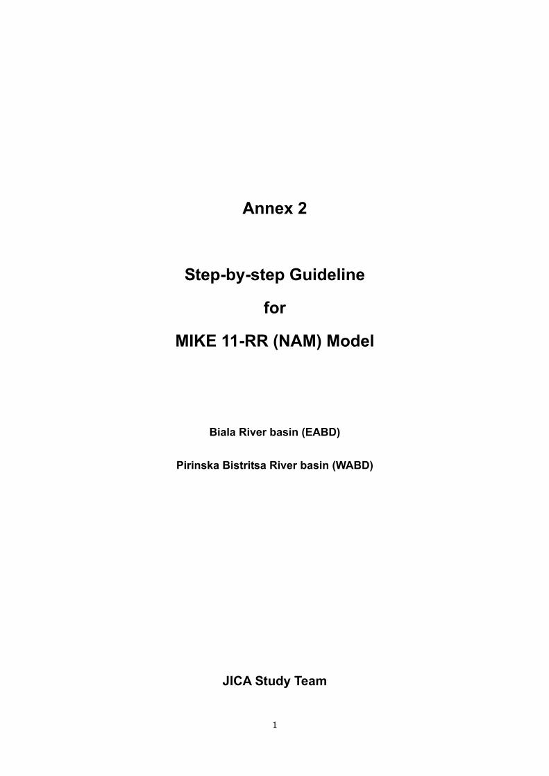
Place cursor on the point at
upstream end, and then right click.
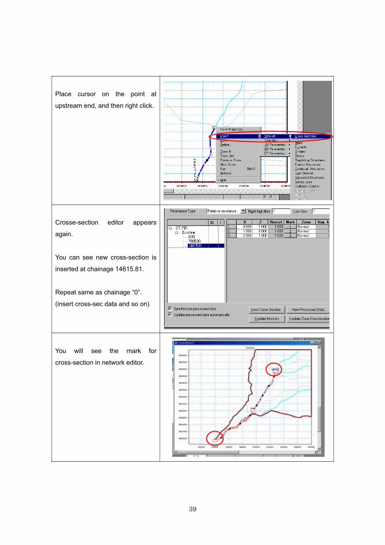
Crosse-section editor appears
again.
You can see new cross-section is
inserted at chainage 14615.81.
Repeat same as chainage “0”.
(insert cross-sec data and so on)
You will see the mark for
cross-section in network editor.

40
Setting .bnd11 file
In network editor, zoom in to
downstream end point using “zoom
in tool”.
Place cursor on the point at
downstream end, and then right
click.
After dialog appears,
Select
Insert -> Boundary -> Hydro
Dynamic
Boundary editor appears.
Set Boundary Description as
“Open”.
Set Boundary Type as “Q-h”.
Make sure “Include HD calculation”
is checked.

41
Highlight h –Q columns.
Tools -> Auto calculation of Q/h
Table
Select Manning formula
Set values for slope and Manning’s
M.

42
h-Q relation is automatically
calculated.
Highlight line 1, then press “Insert”
button in your key board.
New line is inserted.
Insert “0.001” at Q column, line 2.
Select line 11, then press “Tab”
button in your key board.
You will get new line 12.
Insert “100”(big number) at h
column.
Insert “10000”(big number) at Q
column”.
These are for preventing stopping
simulation caused by initial
instability.

43
In network editor, zoom in to
upstream end point using “zoom in
tool”.
Place cursor on the point at
upstream end, and then right click.
After dialog appears,
Select
Insert -> Boundary -> Hydro
Dynamic
Now, you have new boundary “2”.
Set Boundary Description as
“Open”.
Set Boundary Type as “Inflow”.
Make sure “Include HD calculation”
is checked.
Select “Constant” for TS Type.

44
Set values for constant discharge
as “0.001”.
(After you enter the value, you
should press “return” key.)
Note:
In this exercise, RR-HD link will be
applied. Therefore, inlet
discharge can be zero. However,
it is better to give very small
amount of discharge at upstream
end for stabilizing simulation.
Save the .bnd11 file and close it.

45
4. Preparation of Initial Hot start file
MIKE11-HD becomes easily unstable when it starts from rough estimation of initial
condition such as approximation of uniform flow condition.
To prevent this instability, very small time step is required. However, it is not so good
idea to use so small time step for entire simulation.
MIKE11-HD has several options for time-step. Adaptive time-step can work very well
for changing time step automatically corresponding to the requirement to prevent
instability of simulation. However, when RR-HD link is applied, you can not use the
option “Adaptive time-step”.
To overcome this situation, you have to prepare “Initial Hot start file”.
After you prepare “Initial Hot start file”, you can use relatively large time step with option
“fixed time step” without the initial instability.

46
In Project Explorer,
Select
001_Biala/Biala/Biala.bnd11
Then, right click
Select “Copy”.
New file “Copy_Biala.bnd11”
appears in Project Explorer.
Right click it m select ”Rename”.
Rename it to “Biala_int.bnd11”
Double click “Biala_int.bnd11”

47
Activate boundary item”2”.
Set constant discharge value as
“1”.
Save the .bnd11 file, and close it.
In Project Explorer, select
“Biala.sim11”, then double click to
start it.
After network editor appears, select
tab”Input”.
Click”…” for Boundary data.
Select “Baial_int.bnd11” from
Dialog “File selection”.
Then, click “OK”.

48
Select tab ”Simulation”.
Set Time step type as
“Adaptive time step”
Set Simulation period
Start : 2000/01/01
End: 2000/01/02
Set Initial condition for HD as
“Steady State”
Click “Settings..”
After dialog “Time Step Setting”
appears,
Set values as follows
Minimum -> “1”
Maximum ->”300”
Unit -> “Sec.”
Click “OK”.
Note: The above value is based on
experience for EABD & WABD
rivers.
Select tab “Results”.
Set value as follows.
For Storing frequency
“10”.
For Unit
“Time step”
Specify result file name as
“HDint_temp.res11”
Click “OK”.

49
Select tab“Start”.
Click “Start” button.
Simulation completed
Now, you have new result file
“HDint_temp.res11”.
Open it from MIKE View.
You can see the initial development
of flow field.
Check if flow condition is almost
steady at the final time step.
Note:
In this exercise case, 1 day is
enough to get steady state.
However, if total river length is
longer, it may require longer time
period.

50
Select tab “Simulation” from
simulation editor again.
Set Time step type as
“Fixed time step”
Set Time step and unit as
“5” & “ Min”
Set Initial condition for HD
For Type of condition,
“Hotstart”
For Hotstart filename
“/001_Biala/Biala/HDint_temp.res11”
For Hotstart date and Time
“2000/01/01 23:00:00”
Select tab “Results”.
Change result file name as
“HDint_temp2.res11”
Click “OK”.

51
Select tab“Start”.
Click “Start” button.
Now, you can run with relatively
large time step with option “Fixed
time step” without initial instability.
Simulation completed
Now, you have new result file
“HDint_temp2.res11”.
Open it from MIKE View.
Make sure stable condition is
obtained at final time step.

52
Copy “HDint_temp2.res11”
Rename
“copy of HDint_temp2.res11”
to
“HDint_Biala.res11”
Then, move it to folder “INT”.
Now, you are ready for actual
simulation.

53
5. RR-link and run the model
Open “Biala.sim11” from Project
Explore.
Select tab “Model”.
Check ”Hydrodynamic” and
”Rainfall-Runoff”
Select tab “Input”.
Set filename
For Boundary filename
“001_Biala/Biala/Biala.bnd11”
For RR Parameters
“001_Biala/Biala/Biala.RR11”
Click “Edit” for network.

54
After network editor appears,
select
View -> Tabular View
In Tabular View,
select
Runoff/groundwater links
-> Rainfall-runoff links
Open “/003_XLS/RRlink_Biala.xls”
Copy line 2&3

55
In Tabular view of network editor,
Place cursor on any column in line 1.
Press “TAB” key in your key board.
Then, you can insert new line “2”.
Prepare line “1” & “2”.
Note: If number of link is more,
please add more line according to
the number of links.
Highlight NAME to DS chainage
column
Then, paste the copied from .xls file.
Now, RR-HD link are set.

56
Save the .nwk11 file and close it.
Select tab “Simulation”.
Set Time step type as
“Fixed time step”
Set Time step and unit as
“5” & “ Min”
Set Simulation period
Start : 2000/08/01
End: 2006/01/01
Set RR time step multiplier
“144”
Note: Time step of RR is 12hours.
then, 144 = 12 hours x 60min/5min
Set Initial Conditions as follows.
For Type of Condition
“Hotstart”
For Hotstart Filename
“/001_Biala/Biala/INT/HDint_Biala.r
es11”
For Hotstart Date and Time
“2000/01/01 23:00:00”

57
Select tab “Results”.
Set Results filename etc. as
follows.
For HD
Filename:
“001_Biala/Biala/ResultHD/HD_
Biala.res11”
Storing Frequency and Unit
“288” and “time step”
For RR
Filename:
“001_Biala/Biala/ResultRR/RR_
Biala.res11”
Storing Frequency and Unit
“2” and “time step”
Save .sim11 file.
Select tab “Start”.
Click “Start “ button.
Then, simulation will start.
58
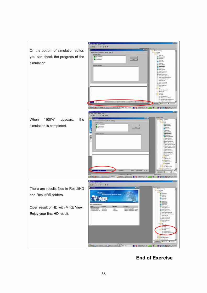
On the bottom of simulation editor,
you can check the progress of the
simulation.
When “100%” appears, the
simulation is completed.
There are results files in ResultHD
and ResultRR folders.
Open result of HD with MIKE View.
Enjoy your first HD result.
End of Exercise