annurev-astro-081309-130914
DESCRIPTION
SPH contributionTRANSCRIPT
AA48CH11-Springel ARI 23 July 2010 15:52
Smoothed ParticleHydrodynamics in AstrophysicsVolker SpringelMax-Planck-Institut fur Astrophysik, D-85741 Garching, Germany;email: [email protected]
Annu. Rev. Astron. Astrophys. 2010. 48:391–430
First published online as a Review in Advance onMay 24, 2010
The Annual Review of Astronomy and Astrophysics isonline at astro.annualreviews.org
This article’s doi:10.1146/annurev-astro-081309-130914
Copyright c© 2010 by Annual Reviews.All rights reserved
0066-4146/10/0922-0391$20.00
Key Words
conservation laws, fluid particles, gas dynamics, numerical convergence,numerical simulations, structure formation
Abstract
This review discusses smoothed particle hydrodynamics (SPH) in the astro-physical context, with a focus on inviscid gas dynamics. The particle-basedSPH technique allows an intuitive and simple formulation of hydrodynamicsthat has excellent conservation properties and can be coupled to self-gravitywith high accuracy. The Lagrangian character of SPH allows it to automat-ically adjust its resolution to the clumping of matter, a property that makesthe scheme ideal for many application areas in astrophysics, where often alarge dynamic range in density is encountered. We discuss the derivation ofthe basic SPH equations in their modern formulation, and give an overviewabout extensions of SPH developed to treat physics such as radiative trans-fer, thermal conduction, relativistic dynamics, or magnetic fields. We alsobriefly describe some of the most important applications areas of SPH in as-trophysical research. Finally, we provide a critical discussion of the accuracyof SPH for different hydrodynamical problems, including measurements ofits convergence rate for important classes of problems.
391
Ann
u. R
ev. A
stro
. Ast
roph
ys. 2
010.
48:3
91-4
30. D
ownl
oade
d fr
om w
ww
.ann
ualr
evie
ws.
org
Acc
ess
prov
ided
by
Uni
vers
ity o
f N
ottin
gham
on
02/0
5/15
. For
per
sona
l use
onl
y.
AA48CH11-Springel ARI 23 July 2010 15:52
1. INTRODUCTION
Smoothed particle hydrodynamics (SPH) is a technique for approximating the continuum dynam-ics of fluids through the use of particles, which may also be viewed as interpolation points. SPHwas originally developed in astrophysics, as introduced by Lucy (1977) and Gingold & Monaghan(1977) some 30 years ago. Since then it has also found widespread use in other areas of science andengineering. In this review, I discuss SPH in its modern form, based on a formulation derived fromvariational principals, giving SPH very good conservation properties and making its derivationlargely free of ad hoc choices that needed to be made in older versions of SPH.
A few excellent reviews have discussed SPH previously (e.g., Monaghan 1992, 2005; Dolag et al.2008; Rosswog 2009); hence, we concentrate primarily on recent developments and on a criticaldiscussion of SPH’s advantages and disadvantages, rather than on giving a full historical account ofthe most important literature on SPH. Also, we generally restrict the discussion of SPH to inviscidideal gases, which is the relevant case for the most common applications in astrophysics, especiallyin cosmology. Only in passing we comment on some other important uses of SPH in astronomy,where fluids quite different from an ideal gas are modeled, e.g., in planet formation. Fully outsidethe scope of this review are the many successful applications of SPH-based techniques in fieldssuch as geophysics and engineering. For example, free-surface flows tend to be very difficult tomodel with Eulerian methods, whereas this is comparatively easy with SPH. As a result, there aremany applications of SPH to problems such as dam-braking, avalanches, and the like, which wehowever do not discuss here.
Numerical simulations have become an important tool in astrophysical research. For example,cosmological simulations of structure formation within the �CDM model have been instrumentalto understanding the nonlinear outcome of the initial conditions predicted by the theory of infla-tion. By now, techniques to simulate collisionless dark matter through the particle-based N-bodymethod (Hockney & Eastwood 1981) have fully matured and are comparatively well understood.However, to represent the collisional baryons as well, the hydrodynamical fluid equations needto be solved, which represents a much harder problem than the dark matter dynamics. On topof the more complicated gas dynamics, additional physics, like radiation fields, magnetic fields,or nonthermal particle components need to be numerically followed as well to produce realisticmodels of the formation and evolution of galaxies, stars, or planets. There is therefore ample needfor robust, accurate, and efficient hydrodynamical discretization techniques in astrophysics.
The principal idea of SPH is to treat hydrodynamics in a completely mesh-free fashion, interms of a set of sampling particles. Hydrodynamical equations of motion are then derived forthese particles, yielding a quite simple and intuitive formulation of gas dynamics. Moreover, itturns out that the particle representation of SPH has excellent conservation properties. Energy,linear momentum, angular momentum, mass, and entropy (if no artificial viscosity operates) aresimultaneously conserved. In addition, there are no advection errors in SPH, and the scheme isfully Galilean invariant, unlike alternative mesh-based Eulerian techniques. Due to its Lagrangiancharacter, the local resolution of SPH follows the mass flow automatically, a property that is ex-tremely convenient in representing the large density contrasts often encountered in astrophysicalproblems. Together with the ease with which SPH can be combined with accurate treatments ofself-gravity (suitable and efficient gravity solvers for particles can be conveniently taken from a cos-mological N-body code developed for the representation of dark matter), this has made the methodvery popular for studying a wide array of problems in astrophysics, ranging from cosmologicalstructure growth driven by gravitational instability to studies of the collisions of protoplanets.Furthermore, additional subresolution treatments of unresolved physical processes (such as starformation in galaxy-scale simulations) can be intuitively added at the particle level in SPH.
392 Springel
Ann
u. R
ev. A
stro
. Ast
roph
ys. 2
010.
48:3
91-4
30. D
ownl
oade
d fr
om w
ww
.ann
ualr
evie
ws.
org
Acc
ess
prov
ided
by
Uni
vers
ity o
f N
ottin
gham
on
02/0
5/15
. For
per
sona
l use
onl
y.
AA48CH11-Springel ARI 23 July 2010 15:52
In this review, we first give, in Section 2, a derivation of what has become the standard for-mulation of SPH for ideal gases, including also a description of the role of artificial viscosity. Wethen summarize some extensions of SPH to include additional physics such as magnetic fieldsor thermal conduction in Section 3, followed by a brief description of the different applicationareas of SPH in astronomy in Section 4. Despite the popularity of SPH, there have been few sys-tematic studies of the accuracy of SPH when compared with the traditional Eulerian approaches.We therefore include a discussion of the convergence, consistency, and stability of standard SPHin Section 5, based on some of our own tests. Finally, we give a discussion of potential futuredirections of SPH development in Section 6 and our conclusions in Section 7.
2. BASIC FORMULATION OF SMOOTHED PARTICLEHYDRODYNAMICS FOR IDEAL GASES
2.1. Kernel Interpolants
At the heart of SPH lie so-called kernel interpolants, which are discussed in detail by Gingold &Monaghan (1982). In particular, we use a kernel summation interpolant for estimating the density,which then determines the rest of the basic SPH equations through the variational formalism.
For any field F(r), we may define a smoothed interpolated version, Fs(r), through a convolutionwith a kernel W(r, h):
Fs (r) =∫
F (r)W (r − r′, h)dr′. (1)
Here, h describes the characteristic width of the kernel, which is normalized to unity and approx-imates a Dirac δ-function in the limit h → 0. We further require that the kernel be symmetricand sufficiently smooth to make it differentiable at least twice. One possibility for W is a Gaussian,which was in fact used by Gingold & Monaghan (1977). However, most current SPH imple-mentations are based on kernels with a finite support. Usually a cubic spline is adopted withW (r, h) = w( |r|
2h ), and
w3D(q ) = 8π
⎧⎪⎨⎪⎩
1 − 6q 2 + 6q 3, 0 ≤ q ≤ 12 ,
2(1 − q )3, 12 < q ≤ 1,
0, q > 1,
(2)
in 3D normalization. This kernel belongs to a broader class of interpolation and smoothing kernels(Schoenberg 1969, Hockney & Eastwood 1981, Monaghan 1985). Note that in the above mostcommonly used definition of the smoothing length h, the kernel drops to zero at a distance ofr = 2h. Through Taylor expansion, it is easy to see that the kernel interpolant is at least second-order accurate due to the symmetry of the kernel.
Suppose now we know the field at a set of points ri; that is, Fi = F (ri ). The points have anassociated mass mi and density ρ i, such that �ri ∼ mi/ρi is their associated finite volume element.Provided the points sufficiently densely sample the kernel volume, we can approximate the integralin Equation 1 with the sum
Fs (r) �∑
j
m j
ρ jFj W (r − r j , h). (3)
This is effectively a Monte-Carlo integration, except that thanks to the comparatively regulardistribution of points encountered in practice, the accuracy is considerably better than for arandom distribution of the sampling points. In particular, for points in one dimension with equalspacing d, one can show that for h = d the sum of Equation 3 provides a second-order accurate
www.annualreviews.org • Smoothed Particle Hydrodynamics 393
Ann
u. R
ev. A
stro
. Ast
roph
ys. 2
010.
48:3
91-4
30. D
ownl
oade
d fr
om w
ww
.ann
ualr
evie
ws.
org
Acc
ess
prov
ided
by
Uni
vers
ity o
f N
ottin
gham
on
02/0
5/15
. For
per
sona
l use
onl
y.
AA48CH11-Springel ARI 23 July 2010 15:52
approximation to the real underlying function. Unfortunately, for the irregular yet somewhatordered particle configurations encountered in real applications, a formal error analysis is notstraightforward. It is clear, however, that at the very least one should have h ≥ d , which translatesto a minimum of ∼33 neighbors in three dimensions.
Importantly, we see that the estimate for Fs (r) is defined everywhere (not only at the underlyingpoints) and is differentiable thanks to the differentiability of the kernel, albeit with a considerablyhigher interpolation error for the derivative. Moreover, if we set F (r) = ρ(r), we obtain
ρs (r) �∑
j
m j W (r − r j , h), (4)
yielding a density estimate based just on the particle coordinates and their masses. In general,the smoothing length can be made variable in space, h = h(r, t), to account for variations in thesampling density. This adaptivity is one of the key advantages of SPH and is essentially alwaysused in practice. There are two options to introduce the variability of h into Equation 4. One isby adopting W [r − r j , h(r)] as kernel, which corresponds to the scatter approach (Hernquist &Katz 1989). It has the advantage that the volume integral of the smoothed field recovers the totalmass,
∫ρs (r)dr = ∑
i mi . However, the so-called gather approach, where we use W [r − r j , h(ri )]as kernel in Equation 4, requires only knowledge of the smoothing length hi for estimating thedensity of particle i, which leads to computationally convenient expressions when the variationof the smoothing length is consistently included in the SPH equations of motion. Because thedensity is only needed at the coordinates of the particles and the total mass is conserved anyway(because it is tied to the particles), it is not important that the volume integral of the gather formof ρs (r) exactly equals the total mass.
In the following, we drop the subscript s for indicating the smoothed field, and adopt as theSPH estimate of the density of particle i the expression
ρi =N∑
j=1
m j W (ri − r j , hi ). (5)
It is clear now why kernels with a finite support are preferred. They allow the summation to berestricted to the Nngb neighbors that lie within the spherical region of radius 2h around the targetpoint ri, corresponding to a computational cost of order O(N ngb N ) for the full density estimate.Normally this number Nngb of neighbors within the support of the kernel is approximately (orexactly) kept constant by choosing the hi appropriately. Nngb, hence, represents an importantparameter of the SPH method and needs to be made large enough to provide sufficient samplingof the kernel volumes. Kernels like the Gaussian, however, would require a summation over allparticles N for every target particle, resulting in an O(N 2) scaling of the computational cost.
If SPH were really a Monte-Carlo method, the accuracy expected from the interpolation errorsof the density estimate would be rather problematic. But the errors are much smaller because theparticles do not sample the fluid in a Poissonian fashion. Instead, their distances tend to equilibratedue to the pressure forces, which makes the interpolation errors much smaller. Yet, they remaina significant source of error in SPH and are ultimately the primary origin of the noise inherent inSPH results.
Even though we have based most of the above discussion on the density, the general kernelinterpolation technique can also be applied to other fields and to the construction of differentialoperators. For example, we may write down a smoothed velocity field and take its derivative to
394 Springel
Ann
u. R
ev. A
stro
. Ast
roph
ys. 2
010.
48:3
91-4
30. D
ownl
oade
d fr
om w
ww
.ann
ualr
evie
ws.
org
Acc
ess
prov
ided
by
Uni
vers
ity o
f N
ottin
gham
on
02/0
5/15
. For
per
sona
l use
onl
y.
AA48CH11-Springel ARI 23 July 2010 15:52
estimate the local velocity divergence, yielding the following:
(∇ · v)i =∑
j
m j
ρ jv j · ∇i W (ri − r j , h). (6)
However, an alternative estimate can be obtained by considering the identity ρ∇·v = ∇(ρv)−v·∇ρ
and computing kernel estimates for the two terms on the right-hand side independently. Theirdifference then yields
(∇ · v)i = 1ρi
∑j
m j (v j − vi ) · ∇i W (ri − r j , h). (7)
This pair-wise formulation turns out to be more accurate in practice. In particular, it has theadvantage of always providing a vanishing velocity divergence if all particle velocities are equal.
2.2. Variational Derivation
The Euler equations for inviscid gas dynamics in Lagrangian (comoving) form are given by
dρ
dt+ ρ∇ · v = 0, (8)
dvdt
+ ∇ Pρ
= 0, (9)
dudt
+ P∇ · v = 0, (10)
where d/dt = ∂/∂t +v ·∇ is the convective derivative. This system of partial differential equationsexpresses conservation of mass, momentum, and energy. Eckart (1960) has shown that the Eulerequations for an inviscid ideal gas follow from the Lagrangian
L =∫
ρ
(v2
2− u
)dV . (11)
This opens up an interesting route for obtaining discretized equations of motion for gas dynamics.Instead of working with the continuum equations directly and trying to heuristically work outa set of accurate difference formulas, one can discretize the Lagrangian and then derive SPHequations of motion by applying the variational principles of classical mechanics, an approachfirst proposed by Gingold & Monaghan (1982). Using a Lagrangian also immediately guaranteescertain conservation laws and retains the geometric structure imposed by Hamiltonian dynamicson phase space.
We here follow this elegant idea, which was first worked out by Springel & Hernquist (2002),with a consistent accounting of variable smoothing lengths. We start by discretizing the Lagrangianin terms of fluid particles of mass mi, yielding
LSPH =∑
i
(12
mi v2i − mi ui
), (12)
where it has been assumed that the thermal energy per unit mass of a particle can be expressedthrough an entropic function Ai of the particle, which simply labels its specific thermodynamicentropy. The pressure of the particles is
Pi = Aiργ
i = (γ − 1)ρi ui , (13)
www.annualreviews.org • Smoothed Particle Hydrodynamics 395
Ann
u. R
ev. A
stro
. Ast
roph
ys. 2
010.
48:3
91-4
30. D
ownl
oade
d fr
om w
ww
.ann
ualr
evie
ws.
org
Acc
ess
prov
ided
by
Uni
vers
ity o
f N
ottin
gham
on
02/0
5/15
. For
per
sona
l use
onl
y.
AA48CH11-Springel ARI 23 July 2010 15:52
where γ is the adiabatic index. Note that for isentropic flow (that is, in the absence of shocks, andwithout mixing or thermal conduction), we expect the Ai to be constant. We, hence, define ui, thethermal energy per unit mass, in terms of the density estimate as
ui (ρi ) = Aiρ
γ−1i
γ − 1. (14)
This raises the question of how the smoothing lengths hi needed for estimating ρ i should bedetermined. As we discussed above, we would like to ensure adaptive kernel sizes, meaning thatthe number of points in the kernel should be approximately constant. In much of the older SPHliterature, the number of neighbors was allowed to vary within some (small) range around a targetnumber. Sometimes the smoothing length itself was evolved with a differential equation in time,exploiting the continuity relation and the expectation that ρh3 should be approximately constant(e.g., Steinmetz & Mueller 1993). In case the number of neighbors inside the kernel happened tofall outside the allowed range, h was suitably readjusted. However, Nelson & Papaloizou (1994)pointed out that for smoothing lengths varied in this way, the energy is not conserved correctly.They showed that the errors could be made smaller by keeping the number of neighbors exactlyconstant, and they also derived leading order correction terms (which became known as ∇h terms)for the classic SPH equations of motion that could reduce them still further. In the modernformulation discussed below, these ∇h terms do not occur; they are implicitly included at allorders.
The central trick making this possible is to require that the mass in the kernel volume shouldbe constant, e.g.,
ρi h3i = const (15)
for three dimensions. Because ρi = ρi (r1, r2, . . . rN , hi ) is only a function of the particle coordinatesand of hi, this equation implicitly defines the function hi = hi (r1, r2, . . . rN ) in terms of the particlecoordinates.
We can then proceed to derive the equations of motion from
ddt
∂L∂ ri
− ∂L∂ri
= 0. (16)
This first gives
midvi
dt= −
N∑j=1
m jPj
ρ2j
∂ρ j
∂ri, (17)
where the derivative ∂ρ j /∂ri stands for the total variation of the density with respect to thecoordinate ri, including any variation of hj this may entail. We can then write
∂ρ j
∂ri= ∇iρ j + ∂ρ j
∂h j
∂h j
∂ri, (18)
where the smoothing length is kept constant in the first derivative on the right-hand side (inour notation, the Nabla operator ∇i = ∂/∂ri means differentiation with respect to ri holding thesmoothing lengths constant). However, differentiation of ρ j h3
j = const with respect to ri yields
∂ρ j
∂h j
∂h j
∂ri
[1 + 3ρ j
h j
(∂ρ j
∂h j
)−1]
= −∇iρ j . (19)
Combining Equations 18 and 19, we then find
∂ρ j
∂ri=
(1 + h j
3ρ j
∂ρ j
∂h j
)−1
∇iρ j . (20)
396 Springel
Ann
u. R
ev. A
stro
. Ast
roph
ys. 2
010.
48:3
91-4
30. D
ownl
oade
d fr
om w
ww
.ann
ualr
evie
ws.
org
Acc
ess
prov
ided
by
Uni
vers
ity o
f N
ottin
gham
on
02/0
5/15
. For
per
sona
l use
onl
y.
AA48CH11-Springel ARI 23 July 2010 15:52
Using
∇iρ j = mi∇i Wi j (h j ) + δi j
N∑k=1
mk∇i Wki (hi ), (21)
we finally obtain the equations of motion
dvi
dt= −
N∑j=1
m j
[fi
Pi
ρ2i∇i Wi j (hi ) + f j
Pj
ρ2j∇i Wi j (h j )
], (22)
where the fi are defined by
fi =[
1 + hi
3ρi
∂ρi
∂hi
]−1
, (23)
and the abbreviation Wi j (h) = W (|ri −r j |, h) has been used. Note that the correction factors fi canbe easily calculated alongside the density estimate; all that is required is an additional summationto get ∂ρi/∂ri for each particle. This quantity is in fact also useful to get the correct smoothingradii by iteratively solving ρi h3
i = const with a Newton-Raphson iteration.The equations of motion (Equation 22) for inviscid hydrodynamics are remarkably simple. In
essence, we have transformed a complicated system of partial differential equations into a muchsimpler set of ordinary differential equations. Furthermore, we only have to solve the momentumequation explicitly. The mass conservation equation as well as the total energy equation (and,hence, the thermal energy equation) are already taken care of, because the particle masses andtheir specific entropies stay constant for reversible gas dynamics. However, later we introduce anartificial viscosity that is needed to allow a treatment of shocks. This introduces additional termsin the equations of motion and requires the time integration of one thermodynamic quantity perparticle, which can be chosen as either entropy or thermal energy. Indeed, Monaghan (2002)pointed out that the above formulation can also be equivalently expressed in terms of thermalenergy instead of entropy. This follows by taking the time derivative of Equation 14, which firstyields
dui
dt= Pi
ρi
∑j
v j · ∂ρi
∂r j. (24)
Using Equations 20 and 21 then gives the evolution of the thermal energy as
dui
dt= fi
Pi
ρi
∑j
m j (vi − v j ) · ∇Wi j (hi ), (25)
which needs to be integrated along the equation of motion if one wants to use the thermal energyas an independent thermodynamic variable. There is no difference, however, between using theentropy or the energy; the two are completely equivalent in the variational formulation. Thisalso solves the old problem pointed out by Hernquist (1993): that the classic SPH equations didnot properly conserve energy when the entropy was integrated, and vice versa. Arguably, it isnumerically advantageous to integrate the entropy though, as this is computationally cheaper andeliminates time integration errors in solving Equation 25.
Note that the above formulation readily fulfills the conservation laws of energy, momentum,and angular momentum. This can be shown based on the discretized form of the equations, but it isalso manifest due to the symmetries of the Lagrangian that was used as a starting point. The absenceof an explicit time dependence gives the energy conservation, the translational invariance impliesmomentum conservation, and the rotational invariance gives angular momentum conservation.
Other derivations of the SPH equations based on constructing kernel interpolated versions ofdifferential operators and applying them directly to the Euler equations are also possible (see, e.g.,
www.annualreviews.org • Smoothed Particle Hydrodynamics 397
Ann
u. R
ev. A
stro
. Ast
roph
ys. 2
010.
48:3
91-4
30. D
ownl
oade
d fr
om w
ww
.ann
ualr
evie
ws.
org
Acc
ess
prov
ided
by
Uni
vers
ity o
f N
ottin
gham
on
02/0
5/15
. For
per
sona
l use
onl
y.
AA48CH11-Springel ARI 23 July 2010 15:52
Monaghan 1992). However, these derivations of “classic SPH” are not unique in the sense that oneis left with several different possibilities for the equations and certain ad hoc symmetrizations needto be introduced. The choice for a particular formulation then needs to rely on experimentallycomparing the performance of many different variants (Thacker et al. 2000).
2.3. Artificial Viscosity
Even when starting from perfectly smooth initial conditions, the gas dynamics described by theEuler equations may readily produce true discontinuities in the form of shock waves and contactdiscontinuities (Landau & Lifshitz 1959). At such fronts the differential form of the Euler equationsbreaks down, and their integral form (equivalent to the conservation laws) needs to be used. Ata shock front, this yields the Rankine-Hugoniot jump conditions that relate the upstream anddownstream states of the fluid. These relations show that the specific entropy of the gas alwaysincreases at a shock front, implying that in the shock layer itself the gas dynamics can no longerbe described as inviscid. In turn, this also implies that the discretized SPH equations we derivedabove cannot correctly describe a shock for the simple reason that they keep the entropy strictlyconstant.
One thus must allow for a modification of the dynamics at shocks and somehow introduce thenecessary dissipation. This is usually accomplished in SPH by an artificial viscosity. Its purpose isto dissipate kinetic energy into heat and to produce entropy in the process. The usual approach isto parameterize the artificial viscosity in terms of a friction force that damps the relative motionof particles. Through the viscosity, the shock is broadened into a resolvable layer, something thatmakes a description of the dynamics everywhere in terms of the differential form possible. It mayseem a daunting task, though, to somehow tune the strength of the artificial viscosity such that justthe right amount of entropy is generated in a shock. Fortunately, this is relatively unproblematic.Provided the viscosity is introduced into the dynamics in a conservative fashion, the conservationlaws themselves ensure that the right amount of dissipation occurs at a shock front.
What is more problematic is to devise the viscosity such that it is only active when there is reallya shock present. If it also operates outside of shocks, even if only at a weak level, the dynamicsmay begin to deviate from that of an ideal gas.
The viscous force is most often added to the equation of motion as
dvi
dt
∣∣∣∣visc
= −N∑
j=1
m j i j ∇i W i j , (26)
where
W i j = 12
[Wi j (hi ) + Wi j (h j )] (27)
denotes a symmetrized kernel, which some researchers prefer to define as W i j = Wi j ([hi +h j ]/2).Provided the viscosity factor ij is symmetric in i and j, the viscous force between any pair ofinteracting particles will be antisymmetric and along the line joining the particles. Hence, linearmomentum and angular momentum are still preserved. In order to conserve total energy, we needto compensate the work done against the viscous force in the thermal reservoir, described eitherin terms of entropy,
dAi
dt
∣∣∣∣visc
= 12
γ − 1
ργ−1i
N∑j=1
m j i j vi j · ∇i W i j , (28)
398 Springel
Ann
u. R
ev. A
stro
. Ast
roph
ys. 2
010.
48:3
91-4
30. D
ownl
oade
d fr
om w
ww
.ann
ualr
evie
ws.
org
Acc
ess
prov
ided
by
Uni
vers
ity o
f N
ottin
gham
on
02/0
5/15
. For
per
sona
l use
onl
y.
AA48CH11-Springel ARI 23 July 2010 15:52
or in terms of thermal energy per unit mass,
dui
dt
∣∣∣∣visc
= 12
N∑j=1
m j i j vi j · ∇i W i j , (29)
where vi j = vi − v j . There is substantial freedom in the detailed parameterization of the viscosityij. The most commonly used formulation is an improved version of the viscosity introduced byMonaghan & Gingold (1983),
i j ={
[−αc i j μi j + βμ2i j ]/ρi j if vi j · ri j < 0
0 otherwise,(30)
with
μi j = hi j vi j · ri j
|ri j |2 + εh2i j
. (31)
Here, hij and ρ ij denote arithmetic means of the corresponding quantities for the two particlesi and j, with cij giving the mean sound speed. The strength of the viscosity is regulated by theparameters α and β, with typical values in the range of α � 0.5 − 1.0 and the frequent choiceof β = 2α. The parameter ε � 0.01 is introduced to protect against singularities if two particleshappen to get very close.
In this form, the artificial viscosity is basically a combination of a bulk and a von Neumann-Richtmyer viscosity. Historically, the quadratic term in μij has been added to the originalMonaghan-Gingold form to prevent particle penetration in high Mach number shocks. Notethat the viscosity only acts for particles that rapidly approach each other; hence, the entropy pro-duction is always positive definite. Also, the viscosity vanishes for solid-body rotation, but not forpure shear flows. To cure this problem in shear flows, Balsara (1995) suggested adding a correctionfactor to the viscosity, reducing its strength when the shear is strong. This can be achieved bymultiplying ij with a prefactor ( f AV
i + f AVj )/2, where the factors
f AVi = |∇ · v|i
|∇ · v|i + |∇ × v|i (32)
are meant to measure the rate of the local compression in relation to the strength of the local shear(estimated with formulas such as Equation 7). This Balsara switch has often been successfully usedin multidimensional flows and is enabled as default in many SPH codes. We note, however, thatit may be problematic sometimes in cases where shocks and shear occur together, e.g., in obliqueshocks in differentially rotating disks.
In some studies, alternative forms of viscosity have been tested. For example, Monaghan (1997)proposed a modified form of the viscosity based on an analogy to the Riemann problem, whichcan be written as
i j = −α
2v
sigi j wi j
ρi j, (33)
where vsigi j = c i + c j − 3wi j is an estimate of the signal velocity between two particles i and j,
and wi j = vi j · ri j /|ri j | is the relative velocity projected onto the separation vector. This viscosityis identical to Equation 30 if one sets β = 3/2 α and replaces wi j with μi j . The main differencebetween the two viscosities lies therefore in the additional factor of hi j /ri j that μi j carries withrespect to wi j . In Equations 30 and 31, this factor weights the viscous force toward particle pairswith small separations. In fact, after multiplying with the kernel derivative, this weighting is strongenough to make the viscous force in Equation 31 diverge as ∝ 1/ri j for small pair separations upto the limit set by the εh2
i j term.
www.annualreviews.org • Smoothed Particle Hydrodynamics 399
Ann
u. R
ev. A
stro
. Ast
roph
ys. 2
010.
48:3
91-4
30. D
ownl
oade
d fr
om w
ww
.ann
ualr
evie
ws.
org
Acc
ess
prov
ided
by
Uni
vers
ity o
f N
ottin
gham
on
02/0
5/15
. For
per
sona
l use
onl
y.
AA48CH11-Springel ARI 23 July 2010 15:52
Lombardi et al. (1999) have systematically tested different parameterization of viscosity, butin general, the standard form was found to work best. Recently, the use of a tensor artificialviscosity was conjectured by Owen (2004) as part of an attempt to optimize the spatial resolutionof SPH. However, a disadvantage of this scheme is that it breaks the strict conservation of angularmomentum.
In attempting to reduce the numerical viscosity of SPH in regions away from shocks, severalstudies have instead advanced the idea of keeping the functional form of the artificial viscosity, butmaking the viscosity strength parameter α variable in time. Such a scheme was first suggested byMorris (1997), and it was successfully applied for studying astrophysical turbulence more faithfullyin SPH (Dolag et al. 2005b) and to follow neutron star mergers (Rosswog et al. 1999, Rosswog2005). Adopting β = 2α, one may evolve the parameter α individually for each particle with anequation such as
dαi
dt= −αi − αmax
τi+ Si , (34)
where Si is some source function meant to ramp up the viscosity rapidly if a shock is detected, whilethe first term lets the viscosity exponentially decay again to a prescribed minimum value αmin on atimescale τ i. So far, simple source functions like Si = max[−(∇ · v)i , 0] and timescales τi � hi/c i
have been explored, and the viscosity, αi, has often also been prevented from becoming higherthan some prescribed maximum value αmax. It is clear that the success of such a variable α schemedepends critically on an appropriate source function. The form above can still not distinguishpurely adiabatic compression from that in a shock, so is not completely free of creating unwantedviscosity.
2.4. Coupling to Self-Gravity
Self-gravity is extremely important in many astrophysical flows, quite in contrast to other areas ofcomputational fluid dynamics, where only external gravitational fields play a role. It is noteworthythat Eulerian mesh-based approaches do not manifestly conserve total energy if self-gravity isincluded (Muller & Steinmetz 1995, Springel 2010), but it can be easily and accurately incorporatedin SPH.
Arguably the best approach to account for gravity is to include it directly into the discretizedSPH Lagrangian, which has the advantage of also allowing a consistent treatment of variable grav-itational softening lengths. This was first conducted by Price & Monaghan (2007) in the context ofadaptive resolution N-body methods for collisionless dynamics (see also Bagla & Khandai 2009).
Let �(r) = G∑
i miφ(r − ri , εi ) be the gravitational field described by the SPH point set,where εi is the gravitational softening length of particle i. We then define the total gravitationalself-energy of the system of SPH particles as
Epot = 12
∑i
mi�(ri ) = G2
∑i j
mi m j φ(ri j , ε j ). (35)
For SPH including self-gravity, the Lagrangian then becomes
LSPH =∑
i
(12
mi v2i − mi ui
)− G
2
∑i j
mi m j φ(ri j , ε j ). (36)
400 Springel
Ann
u. R
ev. A
stro
. Ast
roph
ys. 2
010.
48:3
91-4
30. D
ownl
oade
d fr
om w
ww
.ann
ualr
evie
ws.
org
Acc
ess
prov
ided
by
Uni
vers
ity o
f N
ottin
gham
on
02/0
5/15
. For
per
sona
l use
onl
y.
AA48CH11-Springel ARI 23 July 2010 15:52
As a result, the equation of motion acquires an additional term due to the gravitational forces,given by:
mi agravi = −∂ Epot
∂ri
= −∑
j
Gmi m jri j
ri j
[φ′(ri j , εi ) + φ′(ri j , ε j )]2
(37)
−12
∑j k
Gm j mk∂φ(r jk, ε j )
∂ε
∂ε j
∂ri,
where φ′(r, ε) = ∂φ/∂r .The first sum on the right-hand side describes the ordinary gravitational force, where the
interaction is symmetrized by averaging the forces in case the softening lengths between an inter-acting pair are different. The second sum gives an additional force component that arises whenthe gravitational softening lengths are a function of the particle coordinates themselves, that is,if one invokes adaptive gravitational softening. This term has to be included to make the systemproperly conservative when spatially adaptive gravitational softening lengths are used (Price &Monaghan 2007).
In most cosmological SPH codes of structure formation, this has usually not been done thusfar, and a fixed gravitational softening was used for collisionless dark matter particles and SPHparticles alike. However, especially in the context of gravitational fragmentation problems, itappears natural, and also indicated by accuracy considerations (Bate & Burkert 1997), to tie thegravitational softening length to the SPH smoothing length, even though some studies cautionagainst this strategy (Williams, Churches & Nelson 2004). Adopting εi = hi and determining thesmoothing lengths as described above, we can calculate the ∂ε j /∂ri = ∂h j /∂ri term by means ofEquations 19 and 21. Defining the quantities
η j = h j
3ρ jf j
∑k
mk∂φ(r j k, h j )
∂h, (38)
where the factors fi are defined as in Equation 23, we can then write the gravitational accelerationcompactly as
dvi
dt
∣∣∣∣grav
= −G∑
j
m jri j
ri j
[φ′(ri j , hi ) + φ′(ri j , h j )]2
+ G2
∑j
m j [ηi∇i Wi j (hi ) + η j ∇i Wi j (h j )]. (39)
This acceleration has to be added to the ordinary SPH equations of motion (Equation 22) dueto the pressure forces, which arise from the first part of the Lagrangian (Equation 36). Note thatthe factors ηj can be conveniently calculated alongside the SPH density estimate. The calculationof the gravitational correction force, that is, the second sum in Equation 39, can then be donetogether with the usual calculation of the SPH pressure forces. Unlike in the primary gravitationalforce, here only the nearest neighbors contribute.
We note that it appears natural to relate the functional form of the gravitational softening tothe shape of the SPH smoothing kernel, even though this is not strictly necessary. If this is done,φ(r, h) is determined as a solution to Poisson’s equation,
∇2φ(r, h) = 4πW (r, h). (40)
www.annualreviews.org • Smoothed Particle Hydrodynamics 401
Ann
u. R
ev. A
stro
. Ast
roph
ys. 2
010.
48:3
91-4
30. D
ownl
oade
d fr
om w
ww
.ann
ualr
evie
ws.
org
Acc
ess
prov
ided
by
Uni
vers
ity o
f N
ottin
gham
on
02/0
5/15
. For
per
sona
l use
onl
y.
AA48CH11-Springel ARI 23 July 2010 15:52
The explicit functional form for φ(r, h) resulting from this identification for the cubic spline kernelis also often employed in collisionless N-body codes and can be found, for example, in the appendixof Springel, Yoshida & White (2001).
2.5. Implementation Aspects
The actual use of the discretized SPH equations in simulation models requires a time-integrationscheme. The Hamiltonian character of SPH allows in principle the use of symplectic integrationschemes (Hairer, Lubich & Wanner 2002; Springel 2005), such as the leapfrog, which respects thegeometric phase-space constraints imposed by the conservation laws and can prevent the build-up of secular integration errors with time. However, because most hydrodynamical problems ofinterest are not reversible anyway, this aspect is less important than in dissipation-free collisionlessdynamics. Hence, any second-order accurate time integration scheme, like a simple Runge-Kuttaor predictor-corrector scheme, may equally well be used. It is common practice to use individualtime steps for the SPH particles, often in a block-structured scheme with particles arranged ina power-of-two hierarchy of time steps (Hernquist & Katz 1989). This greatly increases theefficiency of calculations in systems with large dynamic range in timescale, but can make theoptimum choice of time steps tricky. For example, the standard Courant time step criterion of theform
�ti = CCFLhi
c i, (41)
usually used in SPH, where CCFL ∼ 0.1 − 0.3 is a dimensionless parameter, may not guaranteefine enough time-stepping ahead of a blast wave propagating into very cold gas. This problem canbe avoided with an improved method for determining the sizes of individual time steps (Saitoh &Makino 2009).
If self-gravity is included, one can draw from the algorithms employed in collisionless N-body dynamics to calculate the gravitational forces efficiently, such as tree-methods (Barnes &Hut 1986) or mesh-based gravity solvers. The tree approach, which provides for a hierarchicalgrouping of the particles, can also be used to address the primary algorithmic requirement towrite an efficient SPH code, namely the need to efficiently find the neighboring particles insidethe smoothing kernel of a particle. If this is done naively, by computing the distance to all otherparticles, a prohibitive O(N 2) scaling of the computational cost results. Using a range-searchingtechnique together with the tree, this cost can be reduced to O(N ngb N log N ), independent ofthe particle clustering. To this end, a special walk of the tree is carried out for neighbor searchingin which a tree node is only opened if there is a spatial overlap between the tree node and thesmoothing kernel of the target particle; otherwise the corresponding branch of the tree can beimmediately discarded.
These convenient properties of the tree algorithm have been exploited for the developmentof a number of efficient SPH codes in astronomy; several of them are publicly available andparallelized for distributed memory machines. Among them are TreeSPH (Hernquist & Katz1989; Katz, Weinberg & Hernquist 1996), HYDRA (Pearce & Couchman 1997), GADGET(Springel, Yoshida & White 2001; Springel 2005), GASOLINE (Wadsley, Stadel & Quinn 2004),MAGMA (Rosswog & Price 2007), and VINE (Wetzstein et al. 2009).
3. EXTENSIONS OF SMOOTHED PARTICLE HYDRODYNAMICS
For many astrophysical applications, additional physical processes in the gas phase besides invis-cid hydrodynamics need to be modeled. This includes, for example, magnetic fields, transport
402 Springel
Ann
u. R
ev. A
stro
. Ast
roph
ys. 2
010.
48:3
91-4
30. D
ownl
oade
d fr
om w
ww
.ann
ualr
evie
ws.
org
Acc
ess
prov
ided
by
Uni
vers
ity o
f N
ottin
gham
on
02/0
5/15
. For
per
sona
l use
onl
y.
AA48CH11-Springel ARI 23 July 2010 15:52
processes such as thermal conduction or physical viscosity, or radiative transfer. SPH also needsto be modified for the treatment of fluids that move at relativistic speeds or in relativisticallydeep potentials. Below we give a brief overview of some of the extensions of SPH that have beendeveloped to study this physics.
3.1. Magnetic Fields
Magnetic fields are ubiquitous in astrophysical plasmas, where the conductivity can often beapproximated as being effectively infinite. In this limit one aims to simulate ideal, nonresistivemagnetohydrodynamics (MHD), which is thought to be potentially very important in many situ-ations, in particular in star formation, cosmological structure formation, and accretion disks. Theequations of ideal MHD are composed of the induction equation,
dBdt
= (B · ∇)v − B(∇ · v), (42)
and the magnetic Lorentz force. The latter can be obtained from the Maxwell stress tensor,
Mi j = 14π
(Bi B j − 1
2B2δi j
), (43)
as
Fi = ∂Mi j
∂x j. (44)
Working with the stress tensor is advantageous for deriving equations of motion that are discretizedin a symmetric fashion. The magnetic force F then has to be added to the usual forces from gaspressure and the gravitational field.
First implementations of magnetic forces in SPH date back to Gingold & Monaghan (1977),soon followed by full implementations of MHD in SPH (Phillips & Monaghan 1985). However,a significant problem with MHD in SPH has become apparent early on. The constraint equation∇ · B = 0, which is maintained by the continuum form of the ideal MHD equations, is in generalnot preserved by discretized versions of the equations. Those tend to build up ∇ ·B = 0 errors overtime, corresponding to unphysical magnetic monopole sources. In contrast, in the most modernmesh-based approaches to MHD, so-called constrained transport schemes (Evans & Hawley 1988)are able to accurately evolve the discretized magnetic field while keeping a vanishing divergenceof the field.
Much of the recent research on developing improved SPH realizations of MHD has thereforeconcentrated on constructing formulations that either eliminate the ∇ ·B = 0 error or at least keepit reasonably small (Dolag, Bartelmann & Lesch 1999; Price & Monaghan 2004a,b, 2005; Dolag& Stasyszyn 2009; Price 2010). To this extent, different approaches have been investigated in theliterature, involving periodic field cleaning techniques (e.g., Dedner et al. 2002), formulations ofthe equations that “diffuse away” the ∇ · B = 0 terms if they should arise, or the use of the Eulerpotentials or the vector potential. The latter may seem like the most obvious solution, becausederiving the magnetic field as B = ∇ × A from the vector potential A will automatically create adivergence-free field. However, Price (2010) explored the use of the vector potential in SPH andconcluded that there are substantial instabilities in this approach, rendering it essentially uselessin practice.
Another seemingly clean solution lies in the so-called Euler potentials (also known as Clebschvariables). One may write the magnetic field as the cross product B = ∇α × ∇β of the gradientsof two scalar fields α and β. In ideal MHD, where the magnetic flux is locked into the flow, oneobtains the correct field evolution by simply advecting these Euler potentials α and β with the
www.annualreviews.org • Smoothed Particle Hydrodynamics 403
Ann
u. R
ev. A
stro
. Ast
roph
ys. 2
010.
48:3
91-4
30. D
ownl
oade
d fr
om w
ww
.ann
ualr
evie
ws.
org
Acc
ess
prov
ided
by
Uni
vers
ity o
f N
ottin
gham
on
02/0
5/15
. For
per
sona
l use
onl
y.
AA48CH11-Springel ARI 23 July 2010 15:52
motion of the gas. This suggests a deceptively simple approach to ideal MHD; just construct thefields α and β for a given magnetic field, and then move these scalars along with the gas. Althoughthis has been shown to work reasonably well in a number of simple test problems and also hasbeen used in some real-world applications (Price & Bate 2007, Kotarba et al. 2009), it likely hassignificant problems in general MHD dynamics, as a result of the noise in SPH and the inability ofthis scheme to account for any magnetic reconnection. Furthermore, Brandenburg (2010) pointsout that the use of Euler potentials does not converge to a proper solution in hydromagneticturbulence.
Present formulations of MHD in SPH are, hence, back to discretizing the classic magneticinduction equation. For example, Dolag & Stasyszyn (2009) give an implementation of SPH inthe GADGET code where the magnetic induction equation is adopted as
dBi
dt= fi
ρi
∑j
m j {Bi [vi j · ∇i Wi j (hi )] − vi j [Bi · ∇i Wi j (hi )]} (45)
and the acceleration due to magnetic forces as
dvi
dt=
∑j
m j
[fiMi
ρ2i
· ∇i Wi j (hi ) + f jM j
ρ2j
· ∇i Wi j (h j )
], (46)
where the fi are the correction factors of Equation 23, and Mi is the stress tensor of particle i.Combined with field cleaning techniques (Børve, Omang & Trulsen 2001) and artificial mag-netic dissipation to keep ∇ · B = 0 errors under control, this leads to quite accurate results formany standard tests of MHD, like magnetic shock tubes or the Orszag-Tang vortex. A similarimplementation of MHD in SPH is given in the independent MAGMA code by Rosswog & Price(2007).
3.2. Thermal Conduction
Diffusion processes governed by variants of the equation
dQdt
= D ∇2 Q, (47)
where Q is some conserved scalar field and D is a diffusion constant, require a discretization of theLaplace operator in SPH. This could be done in principle by differentiating a kernel-interpolatedversion of Q twice. However, such a discretization turns out to be quite sensitive to the localparticle distribution, or in other words, it is fairly noisy. It is much better to use an approximationof the ∇2 operator proposed first by Brookshaw (1985), in the form
∇2 Q∣∣i = −2
∑j
m j
ρ j
Q j − Qi
r2i j
ri j · ∇i W i j . (48)
Cleary & Monaghan (1999) and Jubelgas, Springel & Dolag (2004) have used this to constructimplementations of thermal conduction in SPH that allow for spatially variable conductivities.The heat conduction equation,
dudt
= 1ρ
∇(κ∇T ), (49)
where κ is the heat conductivity, can then be discretized in SPH as follows:
dui
dt=
∑j
m j
ρiρ j
(κi + κ j )(T j − Ti )r2
i jri j · ∇i W i j . (50)
404 Springel
Ann
u. R
ev. A
stro
. Ast
roph
ys. 2
010.
48:3
91-4
30. D
ownl
oade
d fr
om w
ww
.ann
ualr
evie
ws.
org
Acc
ess
prov
ided
by
Uni
vers
ity o
f N
ottin
gham
on
02/0
5/15
. For
per
sona
l use
onl
y.
AA48CH11-Springel ARI 23 July 2010 15:52
In this form, the energy exchange between two particles is balanced on a pairwise basis, andheat always flows from higher to lower temperature. Also, it is easy to see that the total entropyincreases in the process. This formulation has been used, for example, to study the influence ofSpitzer conductivity due to electron transport on the thermal structure of the plasma in massivegalaxy clusters (Dolag et al. 2004).
3.3. Physical Viscosity
If thermal conduction is not strongly suppressed by magnetic fields in hot plasmas, then one alsoexpects a residual physical viscosity (a pure shear viscosity in this case). In general, real gasesmay possess both physical bulk and physical shear viscosity. They are then correctly described bythe Navier-Stokes equations and not the Euler equations of inviscid gas dynamics that we havediscussed thus far. The stress tensor of the gas can be written as
σi j = η
(∂vi
∂r j+ ∂v j
∂ri− 2
3δi j
∂vk
∂rk
)+ ζ δi j
∂vk
∂rk, (51)
where η and ζ are the coefficients of shear and bulk viscosity, respectively. The Navier-Stokesequation including gravity is then given by
dvdt
= −∇ Pρ
− ∇� + 1ρ
∇σ . (52)
Sijacki & Springel (2006) have suggested an SPH discretization of this equation, which estimatesthe shear viscosity of particle i based on
dvα
dt
∣∣∣∣i, shear
=∑
j
m j
[ηiσαβ |i
ρ2i
[∇i Wi j (hi )]|β + η j σαβ | j
ρ2j
[∇i Wi j (h j )]|β], (53)
and the bulk viscosity as
dvdt
∣∣∣∣i, bulk
=∑
j
m j
[ζi∇ · vi
ρ2i
∇i Wi j (hi ) + ζ j ∇ · v j
ρ2j
∇i Wi j (h j )
]. (54)
These viscous forces are antisymmetric, and together with a positive definite entropy evolution,
dAi
dt= γ − 1
ργ−1i
[12
ηi
ρiσ 2
i + ζi
ρi(∇ · v)2
], (55)
they conserve total energy. Here, the derivatives of the velocity can be estimated with pair-wiseformulations as in Equation 7.
In some sense, it is actually simpler for SPH to solve the Navier-Stokes equation than theEuler equations. As we discuss in more detail in Section 5.4, this is because the inclusion of anartificial viscosity in SPH makes the scheme problematic for purely inviscid flow, because thistypically introduces a certain level of spurious numerical viscosity also outside of shocks. If thegas has, however, a sizable amount of intrinsic physical viscosity anyway, it becomes much easierto correctly represent the fluid, provided the physical viscosity is larger than the unavoidablenumerical viscosity.
3.4. Radiative Transfer
In many astrophysical problems, like the reionization of the Universe or in first star formation,one would like to self-consistently follow the coupled system of hydrodynamical and radiative
www.annualreviews.org • Smoothed Particle Hydrodynamics 405
Ann
u. R
ev. A
stro
. Ast
roph
ys. 2
010.
48:3
91-4
30. D
ownl
oade
d fr
om w
ww
.ann
ualr
evie
ws.
org
Acc
ess
prov
ided
by
Uni
vers
ity o
f N
ottin
gham
on
02/0
5/15
. For
per
sona
l use
onl
y.
AA48CH11-Springel ARI 23 July 2010 15:52
transfer equations, allowing for a proper treatment of the backreaction of the radiation on thefluid, and vice versa. Unfortunately, the radiative transfer equation is in itself a high-dimensionalpartial differential equation that is extremely challenging to solve in its full generality. The task isto follow the evolution of the specific intensity field,
1c
∂ Iν
∂t+ n · ∇ Iν = −κν Iν + jν, (56)
which is not only a function of spatial coordinates, but also of direction n and of frequency ν.Here jν is a source function and κν is an absorption coefficient, which provide an implicit couplingto the hydrodynamics. Despite the formidable challenge to develop efficient numerical schemesfor the approximate solution of the radiation-hydrodynamical set of equations, the developmentof such codes based on SPH-based techniques has really flourished in recent years, where severalnew schemes have been proposed.
Perhaps the simplest and also oldest approaches are based on flux-limited diffusion approx-imations to radiative transfer in SPH (Whitehouse & Bate 2004, 2006; Whitehouse, Bate &Monaghan 2005; Fryer, Rockefeller & Warren 2006; Viau, Bastien & Cha 2006; Forgan et al.2009). A refinement of this strategy has been proposed by Petkova & Springel (2009), based onthe optically thin variable tensor approximations of Gnedin & Abel (2001). In this approach, theradiative transfer equation is simplified in moment-based form, allowing the radiative transfer tobe described in terms of the local energy density Jν of the radiation,
Jν = 14π
∫Iν d�. (57)
This radiation energy density is then transported with an anisotropic diffusion equation,
1c
∂Jν
∂t= ∂
∂r j
(1κν
∂Jνhi j
∂ri
)− κνJν + jν, (58)
where the matrix hij is the so-called Eddington tensor, which is symmetric and normalized tounit trace. The Eddington tensor encodes information about the angle dependence of the localradiation field, and in which direction, if any, it prefers to diffuse in case the local radiation fieldis highly anisotropic. In the ansatz of Gnedin & Abel (2001), the Eddington tensors are simplyestimated in an optically thin approximation as a 1/r2-weighted sum over all sources, which canbe calculated efficiently for an arbitrary number of sources with techniques familiar from thecalculation of gravitational fields.
Petkova & Springel (2009) derive an SPH discretization of the transport part of this radiativetransfer approximation (described by the first term on the right-hand side) as
∂ N i
∂t=
∑j
wi j (N j − N i ), (59)
where the factors wi j are given by
wi j = 2c mi j
κi j ρi j
rTi j hi j ∇i W i j
r2i j
, (60)
and N i = c 2Jν/(h4Planckν
3) is the photon number associated with particle i. The tensor,
h = 52
h − 12
Tr(h), (61)
is a modified Eddington tensor such that the SPH discretization in Equation 60 correspondsto the correct anisotropic diffusion operator. The exchange described by Equation 59 is photon
406 Springel
Ann
u. R
ev. A
stro
. Ast
roph
ys. 2
010.
48:3
91-4
30. D
ownl
oade
d fr
om w
ww
.ann
ualr
evie
ws.
org
Acc
ess
prov
ided
by
Uni
vers
ity o
f N
ottin
gham
on
02/0
5/15
. For
per
sona
l use
onl
y.

AA48CH11-Springel ARI 23 July 2010 15:52
conserving, and because the matrix wi j is symmetric and positive definite, reasonably fast iterativeconjugate gradient solvers can be used to integrate the diffusion problem implicitly in time in astable fashion.
A completely different approach to combine radiative transfer with SPH has been describedby Pawlik & Schaye (2008), who transport the radiation in terms of emission and receptioncones, from particle to particle. This effectively corresponds to a coarse discretization of the solidangle around each particle. Yet another scheme is given by Nayakshin, Cha & Hobbs (2009),who implemented a Monte Carlo implementation of photon transport in SPH. Here, the pho-tons are directly implemented as virtual particles, thereby providing a Monte Carlo sampling ofthe transport equation. Although this method suffers from the usual Monte Carlo noise limita-tions, only few simplifying assumptions in the radiative transfer equation itself have to be made,and it can therefore be made increasingly more accurate simply by using more Monte-Carlophotons.
Finally, Altay, Croft & Pelupessy (2008) suggested a ray-tracing scheme within SPH, whichessentially implements ideas that are known from so-called long- and short-characteristics methodsfor radiative transfer around point sources in mesh codes. These approaches have the advantage ofbeing highly accurate, but their efficiency rapidly declines with an increasing number of sources.
3.5. Relativistic Dynamics
It is also possible to derive SPH equations for relativistic dynamics from a variational principle(Monaghan & Price 2001), both for special and general relativistic dynamics. This is more elegantthan alternative derivations and avoids some problems inherent in other approaches to relativisticdynamics in SPH (Monaghan 1992; Laguna, Miller & Zurek 1993; Faber & Rasio 2000; Siegler& Riffert 2000; Ayal et al. 2001).
The variational method requires discretizing the Lagrangian,
L = −∫
TμνU νU ν dV , (62)
where Uμ is the four-velocity, and Tμν = (P + e)U νU ν + P ημν is the energy momentum tensorof a perfect fluid with pressure P and rest-frame energy density
e = n m0c 2(
1 + uc 2
). (63)
Here a (−1, 1, 1, 1) signature for the flat metric tensor ημν is used. n is the rest frame numberdensity of particles of mean molecular weight m0, and u is the rest-frame thermal energy per unitmass. In the following, we set c = m0 = 1.
Rosswog (2009) gives a detailed derivation of the resulting equations of motion when thediscretization is done in terms of fluid parcels with a constant number ν i of baryons in SPH-particle i and when variable smoothing lengths are consistently included. In the special-relativisticcase, he derives the equations of motion as
dsi
dt= −
∑j
ν j
[fi
Pi
N 2i∇i Wi j (hi ) + f j
Pj
N 2j∇i Wi j (h j )
], (64)
where the generalized momentum si of particle i is given by
si = γi vi
(1 + ui + Pi
ni
), (65)
www.annualreviews.org • Smoothed Particle Hydrodynamics 407
Ann
u. R
ev. A
stro
. Ast
roph
ys. 2
010.
48:3
91-4
30. D
ownl
oade
d fr
om w
ww
.ann
ualr
evie
ws.
org
Acc
ess
prov
ided
by
Uni
vers
ity o
f N
ottin
gham
on
02/0
5/15
. For
per
sona
l use
onl
y.
AA48CH11-Springel ARI 23 July 2010 15:52
and γ i is the particle’s Lorentz factor. The baryon number densities Ni in the computing frameare estimated just as in Equation 4, except for the replacements ρi → N i and m j → ν j . Similarly,the correction factors fi are defined as in Equation 23 with the same replacements.
One also needs to complement the equation of motion with an energy equation of the form
dεi
dt= −
∑j
ν j
[fi Pi
N 2i
vi · ∇Wi j (hi ) + f j Pj
N 2j
v j · ∇Wi j (h j )
], (66)
where
εi = vi · si + 1 + ui
γi(67)
is a suitably defined relativistic energy variable. These equations conserve the total canonicalmomentum as well as the angular momentum. A slight technical complication arises for this choiceof variables due to the need to recover the primitive fluid variables after each time step from theupdated integration variables si and εi, which requires finding the root of a nonlinear equation.
4. APPLICATIONS OF SMOOTHED PARTICLE HYDRODYNAMICS
The versatility and simplicity of SPH have led to a wide range of applications in astronomy,essentially in every field where theoretical research with hydrodynamical simulations is carriedout. We here provide a brief, necessarily incomplete overview of some of the most prominenttopics that have been studied with SPH.
4.1. Cosmological Structure Formation
Among the most important successes of SPH in cosmology are simulations that have clarified theorigin of the Lyman-α forest in the absorption spectra to distant quasars (e.g., Hernquist et al.1996, Dave et al. 1999), which have been instrumental for testing and interpreting the cold darkmatter cosmology. Modern versions of such calculations use detailed chemical models to studythe enrichment of the intragalactic medium (Oppenheimer & Dave 2006), and the nature of theso-called warm-hot IGM, which presumably contains a large fraction of all cosmic baryons (Daveet al. 2001).
Cosmological simulations with hydrodynamics are also used to study galaxy formation in its fullcosmological context, directly from the primordial fluctuation spectrum predicted by inflationarytheory. This requires the inclusion of radiative cooling and subresolution models for the treatmentof star formation and associated energy feedback processes from supernovae explosions or galacticwinds. A large variety of such models have been proposed (e.g., Springel & Hernquist 2003);some also involve rather substantial changes of SPH, for example, the decoupled version of SPHby Marri & White (2003) for the treatment of multiphase structure in the ISM. Despite theuncertainties such modeling involves and the huge challenge to numerical resolution this problementails, important theoretical results on the clustering of galaxies, the evolution of the cosmic star-formation rate, and the efficiency of galaxy formation as a function of halo mass have been reached.
One important goal of such simulations has been the formation of disk galaxies in a cosmologicalcontext, which has however proven to represent a significant challenge. In recent years, substantialprogress in this area has been achieved, however, where some simulated galaxies have become quiteclose now to the morphology of real spiral galaxies (Governato et al. 2007, Scannapieco et al. 2008).Still, the ratio of the stellar bulge to disk components found in simulations is typically much higherthan in observations, and the physical or numerical origin for this discrepancy is debated.
408 Springel
Ann
u. R
ev. A
stro
. Ast
roph
ys. 2
010.
48:3
91-4
30. D
ownl
oade
d fr
om w
ww
.ann
ualr
evie
ws.
org
Acc
ess
prov
ided
by
Uni
vers
ity o
f N
ottin
gham
on
02/0
5/15
. For
per
sona
l use
onl
y.
AA48CH11-Springel ARI 23 July 2010 15:52
The situation is better for clusters of galaxies, where the most recent SPH simulations havebeen quite successful in reproducing the primary scaling relations that are observed (Borgani et al.2004; Puchwein, Sijacki & Springel 2008; McCarthy et al. 2010). This comes after a long strugglein the literature with the cooling-flow problem, namely the fact that simulated clusters tend toefficiently cool out much of their gas at the center, an effect that is not present in observations inthe predicted strength. The modern solution is to attribute this to a nongravitational heat sourcein the center of galaxies, which is thought to arise from active galactic nuclei. This importantfeedback channel has recently been incorporated in SPH simulations of galaxy clusters (Sijackiet al. 2008).
SPH simulations of cosmic large-scale structure and galaxy clusters are also regularly used tostudy the Sunyaev-Zel’dovich effect (da Silva et al. 2000), the buildup of magnetic fields (Dolag,Bartelmann & Lesch 1999, 2002; Dolag et al. 2005a), or even the production of nonthermalparticle populations in the form of cosmic rays (Pfrommer et al. 2007, Jubelgas et al. 2008). Thelatter also required the development of a technique to detect shock waves on the fly in SPH andto measure their Mach number (Pfrommer et al. 2006).
4.2. Galaxy Mergers
The hierarchical theory of galaxy formation predicts frequent mergers of galaxies, leading to thebuildup of ever larger systems. Such galaxy interactions are also prominently observed in manysystems, such as the Antennae Galaxies NGC 4038/4039. The merger hypothesis (Toomre &Toomre 1972) suggests that the coalescence of two spiral galaxies leads to an elliptical remnantgalaxy, thereby playing a central role in explaining Hubble’s tuning fork diagram for the morphol-ogy of galaxies. SPH simulations of merging galaxies have been instrumental in understandingthis process.
In pioneering work by Hernquist (1989), Barnes & Hernquist (1991), and Mihos & Hernquist(1994, 1996), the occurrence of central nuclear starbursts during mergers was studied in detail.Recently, the growth of supermassive black holes has been added to the simulations (Springel,Di Matteo & Hernquist 2005), making it possible to study the coevolution of black holes andstellar bulges in galaxies. Di Matteo, Springel & Hernquist (2005) demonstrated that the energyoutput associated with accretion regulates the black hole growth and establishes the tight observedrelation between black hole masses and bulge velocity dispersions. Subsequently, these simulationshave been used to develop comprehensive models of spheroid formation and for interpreting theevolution and properties of the cosmic quasar population (Hopkins et al. 2005, 2006).
4.3. Star Formation and Stellar Encounters
On smaller scales, many SPH-based simulations have studied the fragmentation of molecularclouds, star formation, and the initial mass function (Bate 1998; Klessen, Burkert & Bate 1998; Bate& Bonnell 2005; Smith, Clark & Bonnell 2009). This includes also simulations of the formation ofthe first stars in the Universe (Bromm, Coppi & Larson 2002; Yoshida et al. 2006; Clark, Glover& Klessen 2008), which are thought to be very special objects.
In this area, important numerical issues related to SPH have been examined as well. Bate &Burkert (1997) show that the Jeans mass needs to be resolved to guarantee reliable results forgravitational fragmentation, a result that was strengthened by Whitworth (1998), who showedthat, provided h ∼ ε and the Jeans mass is resolved, only physical fragmentation should occur.Special on-the-fly particle splitting methods have been developed in order to guarantee that theJeans mass stays resolved over the course of a simulation (Kitsionas & Whitworth 2002, 2007).
www.annualreviews.org • Smoothed Particle Hydrodynamics 409
Ann
u. R
ev. A
stro
. Ast
roph
ys. 2
010.
48:3
91-4
30. D
ownl
oade
d fr
om w
ww
.ann
ualr
evie
ws.
org
Acc
ess
prov
ided
by
Uni
vers
ity o
f N
ottin
gham
on
02/0
5/15
. For
per
sona
l use
onl
y.
AA48CH11-Springel ARI 23 July 2010 15:52
Also, the ability of SPH to represent driven isothermal turbulence has been studied (Klessen,Heitsch & Mac Low 2000).
Pioneering work on stellar collisions with SPH has been performed by Benz & Hills (1987) andBenz et al. (1990). Some of the most recent work in this area studied quite sophisticated problems,such as relativistic neutron star mergers with an approximate treatment of general relativity andsophisticated nuclear matter equations of state (Rosswog, Ramirez-Ruiz & Davies 2003; Oechslin,Janka & Marek 2007), or the triggering of subluminous supernovae type Ia through collisions ofwhite dwarfs (Pakmor et al. 2010).
4.4. Planet Formation and Accretion Disks
SPH have been successfully employed to study giant planet formation through the fragmentationof protoplanetary disks (Mayer et al. 2002, 2004) and to explore the interaction of high- and low-mass planets embedded in protoplanetary discs (Bate et al. 2003, Lufkin et al. 2004). A numberof works have also used SPH to model accretion disks (Simpson 1995), including studies of spiralshocks in 3D disks (Yukawa, Boffin & Matsuda 1997), accretion of gas onto black holes in viscousaccretion disks (Lanzafame, Molteni & Chakrabarti 1998), or cataclysmic variable systems (Woodet al. 2005).
Another interesting application of SPH lies in simulations of materials with different equa-tions of state, corresponding to rocky and icy materials (Benz & Asphaug 1999). This allows theprediction of the outcome of collisions of bodies with sizes from the scale of centimeters to hun-dreds of kilometers, which has important implications for the fate of small fragments in the SolarSystem or in protoplanetary disks. Finally, such simulation techniques allow calculations of thecollision of protoplanets, culminating in numerical simulations that showed how the Moon mighthave formed by an impact between protoearth and an object a tenth of its mass (Benz, Slattery &Cameron 1986).
5. CONVERGENCE, CONSISTENCY, AND STABILITY OF SMOOTHEDPARTICLE HYDRODYNAMICS
There have been a few code comparisons in the literature between SPH and Eulerian hydrody-namics (Frenk et al. 1999, O’Shea et al. 2005, Tasker et al. 2008), but very few formal studies of theaccuracy of SPH have been carried out. Even most code papers on SPH report only circumstantialevidence for SPH’s accuracy. What is especially missing are rigorous studies of the convergencerate of SPH toward known analytic solutions, which is ultimately one of the most sensitive testsof the accuracy of a numerical method. For example, this may involve measuring the error inthe result of an SPH calculation in terms of an L1 error norm relative to a known solution, asis often done in tests of Eulerian hydrodynamics codes. There is no a priori reason why SPHshould not be subjected to equally sensitive tests to establish whether the error becomes smallerwith increasing resolution (convergence) and whether the convergence occurs toward the correctphysical solution (consistency). Such tests can also provide a good basis to compare the efficiencyof different numerical approaches for a particular type of problem with each other.
In this Section, we discuss a number of tests of SPH in one and two dimensions in order toprovide a basic characterization of the accuracy of “standard SPH” as outlined in Section 2. Ourdiscussion is, in particular, meant to critically address some of the weaknesses of standard SPH,both to clarify the origin of the inaccuracies and to guide the ongoing search for improvementsin the approach. We note that there is already a large body of literature with suggestions forimprovements of standard SPH, ranging from minor modifications, say in the parameterization
410 Springel
Ann
u. R
ev. A
stro
. Ast
roph
ys. 2
010.
48:3
91-4
30. D
ownl
oade
d fr
om w
ww
.ann
ualr
evie
ws.
org
Acc
ess
prov
ided
by
Uni
vers
ity o
f N
ottin
gham
on
02/0
5/15
. For
per
sona
l use
onl
y.
AA48CH11-Springel ARI 23 July 2010 15:52
of the artificial viscosity, to more radical changes, such as outfitting SPH with a Riemann solveror replacing the kernel-interpolation technique with a density estimate based on a Voronoi tes-sellation. We shall summarize some of these attempts in Section 6, but refrain from testing themin detail here.
We note that for all test results reported below, it is well possible that small modificationsin the numerical parameters of the code that was used (GADGET2, Springel 2005) may lead toslightly improved results. However, we expect that this may only reduce the error by a constantfactor as a function of resolution, but is unlikely to significantly improve the order or convergence.The former is very helpful of course, but ultimately represents only cosmetic improvements ofthe results. What is fundamentally much more important is the latter, the order of convergenceof a numerical scheme.
5.1. One-Dimensional Sound Waves
Based on analytic reasoning, Rasio (2000) argued that convergence of SPH for 1D sound wavesrequires increasing both the number of smoothing neighbors and the number of particles, withthe latter increasing faster such that the smoothing length and, hence, the smallest resolved scaledecreases. In fact, he showed that in this limit the dispersion relation of sound waves in onedimension is correctly reproduced by SPH for all wavelengths. He also pointed out that if thenumber of neighbors is kept constant and only the number of particles is increased, then one mayconverge to an incorrect physical limit, implying that SPH is inconsistent in this case.
We note that in practice the requirement of consistency may not be crucially important,provided the numerical result converges to a solution that is close enough to the correct physicalsolution. For example, a common error in SPH for a low number of neighbors is that the densityestimate carries a small bias of up to a percent or so. Although this automatically means that theexact physical value of the density is systematically missed by a small amount, in the majority ofastrophysical applications of SPH, the resulting error will be subdominant compared to othererrors or approximations in the physical modeling, and is therefore not really of concern. In ourconvergence tests below, we therefore stick with the common practice of keeping the numberof smoothing neighbors constant. Note that because we compare to known analytic solutions,possible errors in the dispersion relation will be picked up by the error measures anyway.
We begin with the elementary test of a simple acoustic wave that travels through a periodicbox. To avoid any wave steepening, we consider a very small wave amplitude of �ρ/ρ = 10−6.The pressure of the gas is set to P = 3/5 at unit density, such that the adiabatic sound speed isc s = 1 for a gas with γ = 5/3. We let the wave travel once through the box of unit length andcompare the velocity profile of the final result at time t = 1.0 with the initial conditions in termsof an L1 error norm. We define the latter as
L1 = 1N
∑i
|vi − v(xi )|, (68)
where N is the number of SPH particles, vi is the numerical solution for the velocity of particlei, and v(xi ) is the expected analytic solution for the problem, which is here identical to the initialconditions. Note that we deliberately pick the velocity as error measure, because the densityestimate can be subject to a bias that would then completely dominate the error norm. Thevelocity information on the other hand tells us more faithfully how the wave has moved andwhether it properly returned to its original state.
In Figure 1, we show results for the L1 error norm as a function of the number N of equal-massparticles used to sample the domain, for different numbers of smoothing neighbors. Interestingly,
www.annualreviews.org • Smoothed Particle Hydrodynamics 411
Ann
u. R
ev. A
stro
. Ast
roph
ys. 2
010.
48:3
91-4
30. D
ownl
oade
d fr
om w
ww
.ann
ualr
evie
ws.
org
Acc
ess
prov
ided
by
Uni
vers
ity o
f N
ottin
gham
on
02/0
5/15
. For
per
sona
l use
onl
y.
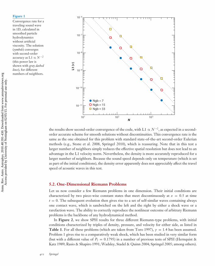
AA48CH11-Springel ARI 23 July 2010 15:52
10 1 10 2 10 3
N
L1 (v
)
10 –11
10 –10
10 –9
10 –8
10 –7
10 –6
Ngb = 7Ngb = 15Ngb = 33
Figure 1Convergence rate for atraveling sound wavein 1D, calculated insmoothed particlehydrodynamicswithout artificialviscosity. The solution(symbols) convergeswith second-orderaccuracy as L1 ∝ N −2
(this power law isshown with gray dashedlines), for differentnumbers of neighbors.
the results show second-order convergence of the code, with L1 ∝ N −2, as expected in a second-order accurate scheme for smooth solutions without discontinuities. This convergence rate is thesame as the one obtained for this problem with standard state-of-the-art second-order Eulerianmethods (e.g., Stone et al. 2008, Springel 2010), which is reassuring. Note that in this test alarger number of neighbors simply reduces the effective spatial resolution but does not lead to anadvantage in the L1 velocity norm. Nevertheless, the density is more accurately reproduced for alarger number of neighbors. Because the sound speed depends only on temperature (which is setas part of the initial conditions), the density error apparently does not appreciably affect the travelspeed of acoustic waves in this test.
5.2. One-Dimensional Riemann Problems
Let us now consider a few Riemann problems in one dimension. Their initial conditions arecharacterized by two piece-wise constant states that meet discontinuously at x = 0.5 at timet = 0. The subsequent evolution then gives rise to a set of self-similar waves containing alwaysone contact wave, which is sandwiched on the left and the right by either a shock wave or ararefaction wave. The ability to correctly reproduce the nonlinear outcome of arbitrary Riemannproblems is the backbone of any hydrodynamical method.
In Figure 2, we show SPH results for three different Riemann-type problems, with initialconditions characterized by triples of density, pressure, and velocity for either side, as listed inTable 1. For all these problems (which are taken from Toro 1997), γ = 1.4 has been assumed.Problem 1 gives rise to a comparatively weak shock, which has been studied in very similar form(but with a different value of P2 = 0.1795) in a number of previous tests of SPH (Hernquist &Katz 1989; Rasio & Shapiro 1991; Wadsley, Stadel & Quinn 2004; Springel 2005; among others).
412 Springel
Ann
u. R
ev. A
stro
. Ast
roph
ys. 2
010.
48:3
91-4
30. D
ownl
oade
d fr
om w
ww
.ann
ualr
evie
ws.
org
Acc
ess
prov
ided
by
Uni
vers
ity o
f N
ottin
gham
on
02/0
5/15
. For
per
sona
l use
onl
y.
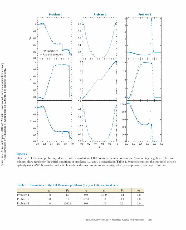
AA48CH11-Springel ARI 23 July 2010 15:52
0.0
0.2
0.4
Problem 1 Problem 2 Problem 3
0.6
0.8
SPH particles
1.0
ρ
Analytic solutions
0.0
0.2
0.4
0.6
0.8
1.0
v
0.0
0.2
0.4
0.6
0.8
1.0
P
0.0 0.2 0.4 0.6 0.8 1.0
0.2
0.4
0.6
0.8
1.0
-2
-1
0
1
2
0.0
0.1
0.2
0.3
0.4
0.5
0.0 0.2 0.4 0.6 0.8 1.0x
1
2
3
4
5
6
0
5
10
15
20
0
200
400
600
800
1,000
0.0 0.2 0.4 0.6 0.8 1.0
Figure 2Different 1D Riemann problems, calculated with a resolution of 100 points in the unit domain, and 7 smoothing neighbors. The threecolumns show results for the initial conditions of problems 1, 2, and 3 as specified in Table 1. Symbols represent the smoothed particlehydrodynamics (SPH) particles, and solid lines show the exact solutions for density, velocity, and pressure, from top to bottom.
Table 1 Parameters of the 1D Riemann problems (for γ = 1.4) examined here
ρ1 P1 ν1 ρ2 P2 ν2
Problem 1 1.0 1.0 0.0 0.125 0.1 0.0Problem 2 1.0 0.4 −2.0 1.0 0.4 2.0Problem 3 1.0 1000.0 0.0 1.0 0.01 0.0
www.annualreviews.org • Smoothed Particle Hydrodynamics 413
Ann
u. R
ev. A
stro
. Ast
roph
ys. 2
010.
48:3
91-4
30. D
ownl
oade
d fr
om w
ww
.ann
ualr
evie
ws.
org
Acc
ess
prov
ided
by
Uni
vers
ity o
f N
ottin
gham
on
02/0
5/15
. For
per
sona
l use
onl
y.
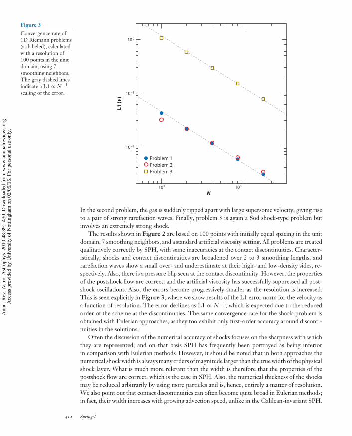
AA48CH11-Springel ARI 23 July 2010 15:52
10 2 10 3
N
L1 (v
)
10 0
10 –1
10 –2
Problem 1Problem 2Problem 3
Figure 3Convergence rate of1D Riemann problems(as labeled), calculatedwith a resolution of100 points in the unitdomain, using 7smoothing neighbors.The gray dashed linesindicate a L1 ∝ N −1
scaling of the error.
In the second problem, the gas is suddenly ripped apart with large supersonic velocity, giving riseto a pair of strong rarefaction waves. Finally, problem 3 is again a Sod shock-type problem butinvolves an extremely strong shock.
The results shown in Figure 2 are based on 100 points with initially equal spacing in the unitdomain, 7 smoothing neighbors, and a standard artificial viscosity setting. All problems are treatedqualitatively correctly by SPH, with some inaccuracies at the contact discontinuities. Character-istically, shocks and contact discontinuities are broadened over 2 to 3 smoothing lengths, andrarefaction waves show a small over- and underestimate at their high- and low-density sides, re-spectively. Also, there is a pressure blip seen at the contact discontinuity. However, the propertiesof the postshock flow are correct, and the artificial viscosity has successfully suppressed all post-shock oscillations. Also, the errors become progressively smaller as the resolution is increased.This is seen explicitly in Figure 3, where we show results of the L1 error norm for the velocity asa function of resolution. The error declines as L1 ∝ N −1, which is expected due to the reducedorder of the scheme at the discontinuities. The same convergence rate for the shock-problem isobtained with Eulerian approaches, as they too exhibit only first-order accuracy around disconti-nuities in the solutions.
Often the discussion of the numerical accuracy of shocks focuses on the sharpness with whichthey are represented, and on that basis SPH has frequently been portrayed as being inferiorin comparison with Eulerian methods. However, it should be noted that in both approaches thenumerical shock width is always many orders of magnitude larger than the true width of the physicalshock layer. What is much more relevant than the width is therefore that the properties of thepostshock flow are correct, which is the case in SPH. Also, the numerical thickness of the shocksmay be reduced arbitrarily by using more particles and is, hence, entirely a matter of resolution.We also point out that contact discontinuities can often become quite broad in Eulerian methods;in fact, their width increases with growing advection speed, unlike in the Galilean-invariant SPH.
414 Springel
Ann
u. R
ev. A
stro
. Ast
roph
ys. 2
010.
48:3
91-4
30. D
ownl
oade
d fr
om w
ww
.ann
ualr
evie
ws.
org
Acc
ess
prov
ided
by
Uni
vers
ity o
f N
ottin
gham
on
02/0
5/15
. For
per
sona
l use
onl
y.
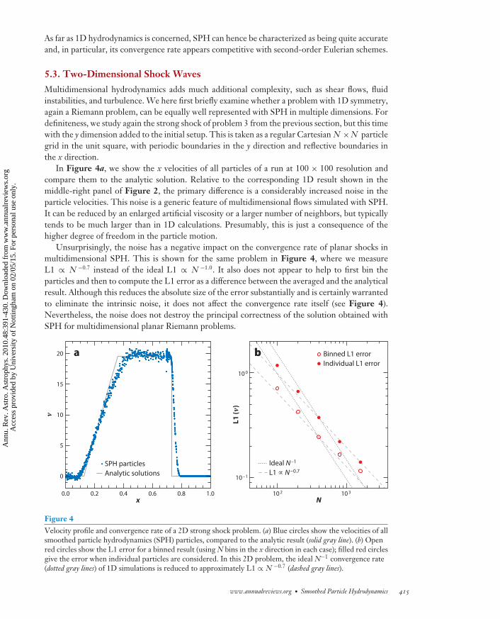
AA48CH11-Springel ARI 23 July 2010 15:52
As far as 1D hydrodynamics is concerned, SPH can hence be characterized as being quite accurateand, in particular, its convergence rate appears competitive with second-order Eulerian schemes.
5.3. Two-Dimensional Shock Waves
Multidimensional hydrodynamics adds much additional complexity, such as shear flows, fluidinstabilities, and turbulence. We here first briefly examine whether a problem with 1D symmetry,again a Riemann problem, can be equally well represented with SPH in multiple dimensions. Fordefiniteness, we study again the strong shock of problem 3 from the previous section, but this timewith the y dimension added to the initial setup. This is taken as a regular Cartesian N × N particlegrid in the unit square, with periodic boundaries in the y direction and reflective boundaries inthe x direction.
In Figure 4a, we show the x velocities of all particles of a run at 100 × 100 resolution andcompare them to the analytic solution. Relative to the corresponding 1D result shown in themiddle-right panel of Figure 2, the primary difference is a considerably increased noise in theparticle velocities. This noise is a generic feature of multidimensional flows simulated with SPH.It can be reduced by an enlarged artificial viscosity or a larger number of neighbors, but typicallytends to be much larger than in 1D calculations. Presumably, this is just a consequence of thehigher degree of freedom in the particle motion.
Unsurprisingly, the noise has a negative impact on the convergence rate of planar shocks inmultidimensional SPH. This is shown for the same problem in Figure 4, where we measureL1 ∝ N −0.7 instead of the ideal L1 ∝ N −1.0. It also does not appear to help to first bin theparticles and then to compute the L1 error as a difference between the averaged and the analyticalresult. Although this reduces the absolute size of the error substantially and is certainly warrantedto eliminate the intrinsic noise, it does not affect the convergence rate itself (see Figure 4).Nevertheless, the noise does not destroy the principal correctness of the solution obtained withSPH for multidimensional planar Riemann problems.
0.0 0.2 0.4 0.6 0.8 1.0x
0
5
10
15
20 a
10 2 10 3
N
10 –1
L1 (v
)
v
10 0
SPH particlesAnalytic solutions
Ideal N–1
L1 ∝ N–0.7
Binned L1 errorIndividual L1 error
bb
Figure 4Velocity profile and convergence rate of a 2D strong shock problem. (a) Blue circles show the velocities of allsmoothed particle hydrodynamics (SPH) particles, compared to the analytic result (solid gray line). (b) Openred circles show the L1 error for a binned result (using N bins in the x direction in each case); filled red circlesgive the error when individual particles are considered. In this 2D problem, the ideal N−1 convergence rate(dotted gray lines) of 1D simulations is reduced to approximately L1 ∝ N −0.7 (dashed gray lines).
www.annualreviews.org • Smoothed Particle Hydrodynamics 415
Ann
u. R
ev. A
stro
. Ast
roph
ys. 2
010.
48:3
91-4
30. D
ownl
oade
d fr
om w
ww
.ann
ualr
evie
ws.
org
Acc
ess
prov
ided
by
Uni
vers
ity o
f N
ottin
gham
on
02/0
5/15
. For
per
sona
l use
onl
y.
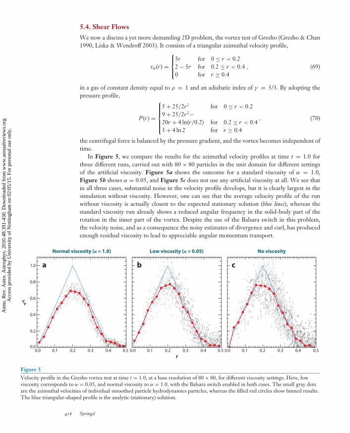
AA48CH11-Springel ARI 23 July 2010 15:52
5.4. Shear Flows
We now a discuss a yet more demanding 2D problem, the vortex test of Gresho (Gresho & Chan1990, Liska & Wendroff 2003). It consists of a triangular azimuthal velocity profile,
vφ(r) =
⎧⎪⎨⎪⎩
5r for 0 ≤ r < 0.22 − 5r for 0.2 ≤ r < 0.40 for r ≥ 0.4
, (69)
in a gas of constant density equal to ρ = 1 and an adiabatic index of γ = 5/3. By adopting thepressure profile,
P (r) =
⎧⎪⎪⎪⎨⎪⎪⎪⎩
5 + 25/2r2 for 0 ≤ r < 0.29 + 25/2r2−20r + 4 ln(r/0.2) for 0.2 ≤ r < 0.43 + 4 ln 2 for r ≥ 0.4
, (70)
the centrifugal force is balanced by the pressure gradient, and the vortex becomes independent oftime.
In Figure 5, we compare the results for the azimuthal velocity profiles at time t = 1.0 forthree different runs, carried out with 80 × 80 particles in the unit domain for different settingsof the artificial viscosity. Figure 5a shows the outcome for a standard viscosity of α = 1.0,Figure 5b shows α = 0.05, and Figure 5c does not use any artificial viscosity at all. We see thatin all three cases, substantial noise in the velocity profile develops, but it is clearly largest in thesimulation without viscosity. However, one can see that the average velocity profile of the runwithout viscosity is actually closest to the expected stationary solution (blue lines), whereas thestandard viscosity run already shows a reduced angular frequency in the solid-body part of therotation in the inner part of the vortex. Despite the use of the Balsara switch in this problem,the velocity noise, and as a consequence the noisy estimates of divergence and curl, has producedenough residual viscosity to lead to appreciable angular momentum transport.
0.0
0.2
0.4
0.6
0.8
1.0
Normal viscosity (α = 1.0)
a b c
0.0 0.1 0.2 0.3 0.4 0.5 0.0 0.1 0.2 0.3 0.4 0.50.0 0.1 0.2 0.3 0.4 0.5r
Low viscosity (α = 0.05) No viscosity
vφ
Figure 5Velocity profile in the Gresho vortex test at time t = 1.0, at a base resolution of 80 × 80, for different viscosity settings. Here, lowviscosity corresponds to α = 0.05, and normal viscosity to α = 1.0, with the Balsara switch enabled in both cases. The small gray dotsare the azimuthal velocities of individual smoothed particle hydrodynamics particles, whereas the filled red circles show binned results.The blue triangular-shaped profile is the analytic (stationary) solution.
416 Springel
Ann
u. R
ev. A
stro
. Ast
roph
ys. 2
010.
48:3
91-4
30. D
ownl
oade
d fr
om w
ww
.ann
ualr
evie
ws.
org
Acc
ess
prov
ided
by
Uni
vers
ity o
f N
ottin
gham
on
02/0
5/15
. For
per
sona
l use
onl
y.
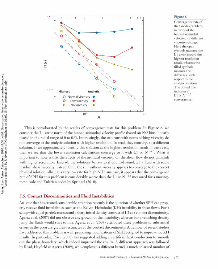
AA48CH11-Springel ARI 23 July 2010 15:52
N10 2 10 3
L1 (v
)
10 –1
10 –2
Normal viscosity
Highest Analytic
Low viscosityNo viscosity
L1 ∝ N –0.7
Figure 6Convergence rate ofthe Gresho problem,in terms of thebinned azimuthalvelocity, for differentviscosity settings.Here the opensymbols measure theL1 error toward thehighest resolutionresult, whereas thefilled symbolsmeasure thedifference withrespect to theanalytic solution.The dotted lineindicates aL1 ∝ N −0.7
convergence.
This is corroborated by the results of convergence tests for this problem. In Figure 6, weconsider the L1 error norm of the binned azimuthal velocity profile (based on N/2 bins, linearlyplaced in the radial range of 0 to 0.5). Interestingly, the two runs with nonvanishing viscosity donot converge to the analytic solution with higher resolution. Instead, they converge to a differentsolution. If we approximately identify this solution as the highest resolution result in each case,then we see that the lower resolution calculations converge to it with L1 ∝ N −0.7. What isimportant to note is that the effects of the artificial viscosity on the shear flow do not diminishwith higher resolution. Instead, the solutions behave as if one had simulated a fluid with someresidual shear viscosity instead. Only the run without viscosity appears to converge to the correctphysical solution, albeit at a very low rate for high N. In any case, it appears that the convergencerate of SPH for this problem is considerably worse than the L1 ∝ N −1.4 measured for a moving-mesh code and Eulerian codes by Springel (2010).
5.5. Contact Discontinuities and Fluid Instabilities
An issue that has created considerable attention recently is the question of whether SPH can prop-erly resolve fluid instabilities, such as the Kelvin-Helmholtz (KH) instability in shear flows. For asetup with equal particle masses and a sharp initial density contrast of 1:2 at a contact discontinuity,Agertz et al. (2007) did not observe any growth of the instability, whereas for a vanishing densityjump the fluids would start to mix. Agertz et al. (2007) attributed these problems to substantialerrors in the pressure gradient estimates at the contact discontinuity. A number of recent studieshave addressed this problem as well, proposing modifications of SPH designed to improve the KHresults. In particular, Price (2008) has suggested adding an artificial heat conduction to smoothout the phase boundary, which indeed improved the results. A different approach was followedby Read, Hayfield & Agertz (2009), who employed a different kernel, a much enlarged number of
www.annualreviews.org • Smoothed Particle Hydrodynamics 417
Ann
u. R
ev. A
stro
. Ast
roph
ys. 2
010.
48:3
91-4
30. D
ownl
oade
d fr
om w
ww
.ann
ualr
evie
ws.
org
Acc
ess
prov
ided
by
Uni
vers
ity o
f N
ottin
gham
on
02/0
5/15
. For
per
sona
l use
onl
y.
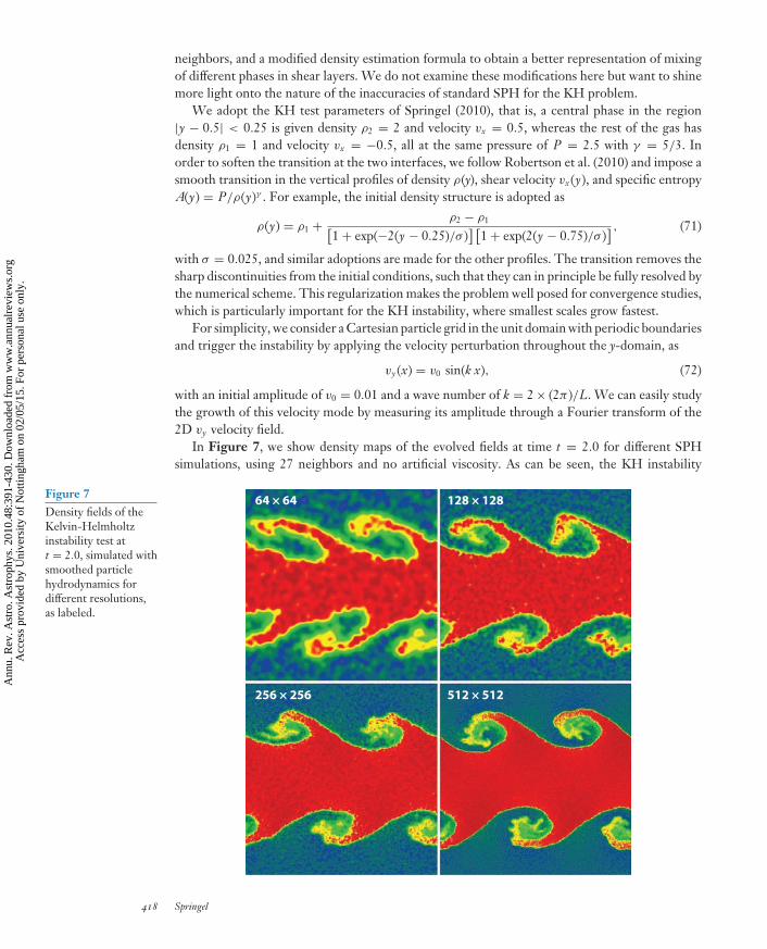
AA48CH11-Springel ARI 23 July 2010 15:52
neighbors, and a modified density estimation formula to obtain a better representation of mixingof different phases in shear layers. We do not examine these modifications here but want to shinemore light onto the nature of the inaccuracies of standard SPH for the KH problem.
We adopt the KH test parameters of Springel (2010), that is, a central phase in the region|y − 0.5| < 0.25 is given density ρ2 = 2 and velocity vx = 0.5, whereas the rest of the gas hasdensity ρ1 = 1 and velocity vx = −0.5, all at the same pressure of P = 2.5 with γ = 5/3. Inorder to soften the transition at the two interfaces, we follow Robertson et al. (2010) and impose asmooth transition in the vertical profiles of density ρ(y), shear velocity vx(y), and specific entropyA(y) = P/ρ(y)γ . For example, the initial density structure is adopted as
ρ(y) = ρ1 + ρ2 − ρ1[1 + exp(−2(y − 0.25)/σ )
] [1 + exp(2(y − 0.75)/σ )
] , (71)
with σ = 0.025, and similar adoptions are made for the other profiles. The transition removes thesharp discontinuities from the initial conditions, such that they can in principle be fully resolved bythe numerical scheme. This regularization makes the problem well posed for convergence studies,which is particularly important for the KH instability, where smallest scales grow fastest.
For simplicity, we consider a Cartesian particle grid in the unit domain with periodic boundariesand trigger the instability by applying the velocity perturbation throughout the y-domain, as
vy (x) = v0 sin(k x), (72)
with an initial amplitude of v0 = 0.01 and a wave number of k = 2 × (2π )/L. We can easily studythe growth of this velocity mode by measuring its amplitude through a Fourier transform of the2D vy velocity field.
In Figure 7, we show density maps of the evolved fields at time t = 2.0 for different SPHsimulations, using 27 neighbors and no artificial viscosity. As can be seen, the KH instability
64 × 64 128 × 128
256 × 256 512 × 512
Figure 7Density fields of theKelvin-Helmholtzinstability test att = 2.0, simulated withsmoothed particlehydrodynamics fordifferent resolutions,as labeled.
418 Springel
Ann
u. R
ev. A
stro
. Ast
roph
ys. 2
010.
48:3
91-4
30. D
ownl
oade
d fr
om w
ww
.ann
ualr
evie
ws.
org
Acc
ess
prov
ided
by
Uni
vers
ity o
f N
ottin
gham
on
02/0
5/15
. For
per
sona
l use
onl
y.
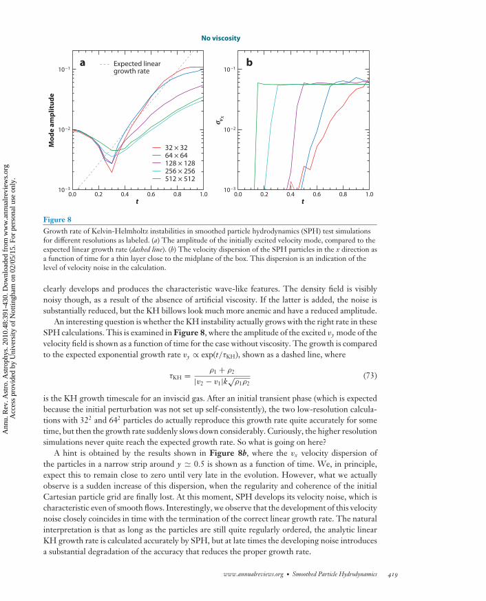
AA48CH11-Springel ARI 23 July 2010 15:52
10 –1
10 –2
10 –3
10 –1
10 –2
10 –3
σ vX
a b
0.0 0.2 0.4 0.6 0.8 1.0t
Mod
e am
plit
ude
0.0 0.2 0.4 0.6 0.8 1.0t
32 × 32
Expected lineargrowth rate
64 × 64128 × 128256 × 256512 × 512
No viscosity
Figure 8Growth rate of Kelvin-Helmholtz instabilities in smoothed particle hydrodynamics (SPH) test simulationsfor different resolutions as labeled. (a) The amplitude of the initially excited velocity mode, compared to theexpected linear growth rate (dashed line). (b) The velocity dispersion of the SPH particles in the x direction asa function of time for a thin layer close to the midplane of the box. This dispersion is an indication of thelevel of velocity noise in the calculation.
clearly develops and produces the characteristic wave-like features. The density field is visiblynoisy though, as a result of the absence of artificial viscosity. If the latter is added, the noise issubstantially reduced, but the KH billows look much more anemic and have a reduced amplitude.
An interesting question is whether the KH instability actually grows with the right rate in theseSPH calculations. This is examined in Figure 8, where the amplitude of the excited vy mode of thevelocity field is shown as a function of time for the case without viscosity. The growth is comparedto the expected exponential growth rate vy ∝ exp(t/τKH), shown as a dashed line, where
τKH = ρ1 + ρ2
|v2 − v1|k√ρ1ρ2
(73)
is the KH growth timescale for an inviscid gas. After an initial transient phase (which is expectedbecause the initial perturbation was not set up self-consistently), the two low-resolution calcula-tions with 322 and 642 particles do actually reproduce this growth rate quite accurately for sometime, but then the growth rate suddenly slows down considerably. Curiously, the higher resolutionsimulations never quite reach the expected growth rate. So what is going on here?
A hint is obtained by the results shown in Figure 8b, where the vx velocity dispersion ofthe particles in a narrow strip around y � 0.5 is shown as a function of time. We, in principle,expect this to remain close to zero until very late in the evolution. However, what we actuallyobserve is a sudden increase of this dispersion, when the regularity and coherence of the initialCartesian particle grid are finally lost. At this moment, SPH develops its velocity noise, which ischaracteristic even of smooth flows. Interestingly, we observe that the development of this velocitynoise closely coincides in time with the termination of the correct linear growth rate. The naturalinterpretation is that as long as the particles are still quite regularly ordered, the analytic linearKH growth rate is calculated accurately by SPH, but at late times the developing noise introducesa substantial degradation of the accuracy that reduces the proper growth rate.
www.annualreviews.org • Smoothed Particle Hydrodynamics 419
Ann
u. R
ev. A
stro
. Ast
roph
ys. 2
010.
48:3
91-4
30. D
ownl
oade
d fr
om w
ww
.ann
ualr
evie
ws.
org
Acc
ess
prov
ided
by
Uni
vers
ity o
f N
ottin
gham
on
02/0
5/15
. For
per
sona
l use
onl
y.
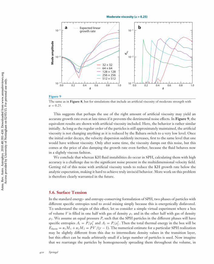
AA48CH11-Springel ARI 23 July 2010 15:52
10 –1
10 –2
10 –3
10 –1
10 –2
10 –3
σ vX
a b
0.0 0.2 0.4 0.6 0.8 1.0t
Mod
e am
plit
ude
0.0 0.2 0.4 0.6 0.8 1.0t
32 × 32
Expected lineargrowth rate
64 × 64128 × 128256 × 256512 × 512
Moderate viscosity (α = 0.25)
Figure 9The same as in Figure 8, but for simulations that include an artificial viscosity of moderate strength withα = 0.25.
This suggests that perhaps the use of the right amount of artificial viscosity may yield anaccurate growth rate even at late times if it prevents the detrimental noise effects. In Figure 9, theequivalent results are shown with artificial viscosity included. Here, the behavior is rather similarinitially. As long as the regular order of the particles is still approximately maintained, the artificialviscosity is not changing anything as it is reduced by the Balsara switch to a very low level. Oncethe initial order decays, the velocity dispersion suddenly increases, first to the same level that onewould have without viscosity. Only after some time, the viscosity damps out this noise, but thiscomes at the price of also damping the growth rate even further, because the fluid behaves nowin a slightly viscous fashion.
We conclude that whereas KH fluid instabilities do occur in SPH, calculating them with highaccuracy is a challenge due to the significant noise present in the multidimensional velocity field.Getting rid of this noise with artificial viscosity tends to reduce the KH growth rate below theanalytic expectation, making it hard to achieve truly inviscid behavior. More work on this problemis therefore clearly warranted in the future.
5.6. Surface Tension
In the standard energy- and entropy-conserving formulation of SPH, two phases of particles withdifferent specific entropies tend to avoid mixing simply because this is energetically disfavored.To understand the origin of this effect, let us consider a simple virtual experiment where a boxof volume V is filled in one half with gas of density ρ1 and in the other half with gas of densityρ2. We assume an equal pressure P, such that the SPH particles in the different phases will havespecific entropies A1 = P/ρ
γ
1 and A2 = P/ργ
2 . Then the total thermal energy in the box will beEtherm = u1 M 1 + u2 M 2 = PV /(γ − 1). The numerical estimate for a particular SPH realizationmay be slightly different from this due to intermediate density values in the transition layer,but this effect can be made arbitrarily small if a large number of particles is used. Now imaginethat we rearrange the particles by homogeneously spreading them throughout the volume, in
420 Springel
Ann
u. R
ev. A
stro
. Ast
roph
ys. 2
010.
48:3
91-4
30. D
ownl
oade
d fr
om w
ww
.ann
ualr
evie
ws.
org
Acc
ess
prov
ided
by
Uni
vers
ity o
f N
ottin
gham
on
02/0
5/15
. For
per
sona
l use
onl
y.
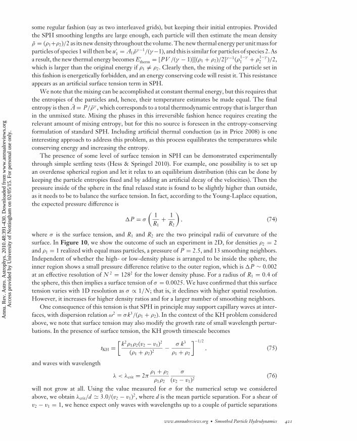
AA48CH11-Springel ARI 23 July 2010 15:52
some regular fashion (say as two interleaved grids), but keeping their initial entropies. Providedthe SPH smoothing lengths are large enough, each particle will then estimate the mean densityρ = (ρ1+ρ2)/2 as its new density throughout the volume. The new thermal energy per unit mass forparticles of species 1 will then be u′
1 = A1ργ−1/(γ −1), and this is similar for particles of species 2. As
a result, the new thermal energy becomes E ′therm = [PV /(γ − 1)][(ρ1 + ρ2)/2]γ−1(ρ1−γ
1 + ρ1−γ
2 )/2,which is larger than the original energy if ρ1 = ρ2. Clearly then, the mixing of the particle set inthis fashion is energetically forbidden, and an energy conserving code will resist it. This resistanceappears as an artificial surface tension term in SPH.
We note that the mixing can be accomplished at constant thermal energy, but this requires thatthe entropies of the particles and, hence, their temperature estimates be made equal. The finalentropy is then A = P/ργ , which corresponds to a total thermodynamic entropy that is larger thanin the unmixed state. Mixing the phases in this irreversible fashion hence requires creating therelevant amount of mixing entropy, but for this no source is foreseen in the entropy-conservingformulation of standard SPH. Including artificial thermal conduction (as in Price 2008) is oneinteresting approach to address this problem, as this process equilibrates the temperatures whileconserving energy and increasing the entropy.
The presence of some level of surface tension in SPH can be demonstrated experimentallythrough simple settling tests (Hess & Springel 2010). For example, one possibility is to set upan overdense spherical region and let it relax to an equilibrium distribution (this can be done bykeeping the particle entropies fixed and by adding an artificial decay of the velocities). Then thepressure inside of the sphere in the final relaxed state is found to be slightly higher than outside,as it needs to be to balance the surface tension. In fact, according to the Young-Laplace equation,the expected pressure difference is
�P = σ
(1R1
+ 1R2
), (74)
where σ is the surface tension, and R1 and R2 are the two principal radii of curvature of thesurface. In Figure 10, we show the outcome of such an experiment in 2D, for densities ρ2 = 2and ρ1 = 1 realized with equal mass particles, a pressure of P = 2.5, and 13 smoothing neighbors.Independent of whether the high- or low-density phase is arranged to be inside the sphere, theinner region shows a small pressure difference relative to the outer region, which is �P ∼ 0.002at an effective resolution of N 2 = 1282 for the lower density phase. For a radius of R1 = 0.4 ofthe sphere, this then implies a surface tension of σ = 0.0025. We have confirmed that this surfacetension varies with 1D resolution as σ ∝ 1/N; that is, it declines with higher spatial resolution.However, it increases for higher density ratios and for a larger number of smoothing neighbors.
One consequence of this tension is that SPH in principle may support capillary waves at inter-faces, with dispersion relation ω2 = σk3/(ρ1 + ρ2). In the context of the KH problem consideredabove, we note that surface tension may also modify the growth rate of small wavelength pertur-bations. In the presence of surface tension, the KH growth timescale becomes
tKH =[
k2ρ1ρ2(v2 − v1)2
(ρ1 + ρ2)2− σ k3
ρ1 + ρ2
]−1/2
, (75)
and waves with wavelength
λ < λcrit = 2πρ1 + ρ2
ρ1ρ2
σ
(v2 − v1)2(76)
will not grow at all. Using the value measured for σ for the numerical setup we consideredabove, we obtain λcrit/d � 3.0/(v2 − v1)2, where d is the mean particle separation. For a shear ofv2 − v1 = 1, we hence expect only waves with wavelengths up to a couple of particle separations
www.annualreviews.org • Smoothed Particle Hydrodynamics 421
Ann
u. R
ev. A
stro
. Ast
roph
ys. 2
010.
48:3
91-4
30. D
ownl
oade
d fr
om w
ww
.ann
ualr
evie
ws.
org
Acc
ess
prov
ided
by
Uni
vers
ity o
f N
ottin
gham
on
02/0
5/15
. For
per
sona
l use
onl
y.
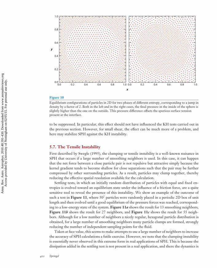
AA48CH11-Springel ARI 23 July 2010 15:52
0.0 0.2 0.4 0.6 0.8 1.0
x
0.0
0.2
0.4
0.6
0.8
1.0
y
0.0 0.2 0.4 0.6 0.8 1.0
Figure 10Equilibrium configurations of particles in 2D for two phases of different entropy, corresponding to a jump indensity by a factor of 2. Both in the left and in the right cases, the final pressure in the inside of the sphere isslightly higher than the one on the outside. This pressure difference offsets the spurious surface tensionpresent at the interface.
to be suppressed. In particular, this effect should not have influenced the KH tests carried out inthe previous section. However, for small shear, the effect can be much more of a problem, andhere may stabilize SPH against the KH instability.
5.7. The Tensile Instability
First described by Swegle (1995), the clumping or tensile instability is a well-known nuisance inSPH that occurs if a large number of smoothing neighbors is used. In this case, it can happenthat the net force between a close particle pair is not repulsive but attractive simply because thekernel gradient tends to become shallow for close separations such that the pair may be furthercompressed by other surrounding particles. As a result, particles may clump together, therebyreducing the effective spatial resolution available for the calculation.
Settling tests, in which an initially random distribution of particles with equal and fixed en-tropies is evolved toward an equilibrium state under the influence of a friction force, are a quitesensitive tool to reveal the presence of this instability. We show an example of the outcome ofsuch a test in Figure 11, where 502 particles were randomly placed in a periodic 2D box of unitlength and then evolved until a good equilibrium of the pressure forces was reached, correspond-ing to a low-energy state of the system. Figure 11a shows the result for 13 smoothing neighbors,Figure 11b shows the result for 27 neighbors, and Figure 11c shows the result for 55 neigh-bors. Although for a low number of neighbors a nicely regular, hexagonal particle distribution isobtained, for a large number of smoothing neighbors many particle clumps are formed, stronglyreducing the number of independent sampling points for the fluid.
Taken at face value, this seems to make attempts to use a large number of neighbors to increasethe accuracy of SPH calculations a futile exercise. However, we note that the clumping instabilityis essentially never observed in this extreme form in real applications of SPH. This is because thedissipation added in the settling test is not present in a real application, and there the dynamics is
422 Springel
Ann
u. R
ev. A
stro
. Ast
roph
ys. 2
010.
48:3
91-4
30. D
ownl
oade
d fr
om w
ww
.ann
ualr
evie
ws.
org
Acc
ess
prov
ided
by
Uni
vers
ity o
f N
ottin
gham
on
02/0
5/15
. For
per
sona
l use
onl
y.
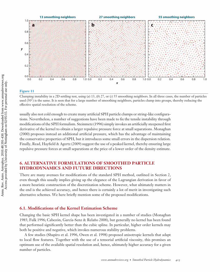
AA48CH11-Springel ARI 23 July 2010 15:52
0.0 0.2 0.4 0.6 0.8 1.00.0
0.2
0.4
0.6
0.8
1.0
0.0 0.2 0.4 0.6 0.8 1.0x
0.0 0.2 0.4 0.6 0.8 1.0
y
13 smoothing neighbors 27 smoothing neighbors 55 smoothing neighbors
a b ca b c
Figure 11Clumping instability in a 2D settling test, using (a) 13, (b) 27, or (c) 55 smoothing neighbors. In all three cases, the number of particlesused (502) is the same. It is seen that for a large number of smoothing neighbors, particles clump into groups, thereby reducing theeffective spatial resolution of the scheme.
usually also not cold enough to create many artificial SPH particle clumps or string-like configura-tions. Nevertheless, a number of suggestions have been made to fix the tensile instability throughmodifications of the SPH formalism. Steinmetz (1996) simply invokes an artificially steepened firstderivative of the kernel to obtain a larger repulsive pressure force at small separations. Monaghan(2000) proposes instead an additional artificial pressure, which has the advantage of maintainingthe conservative properties of SPH, but it introduces some small errors in the dispersion relation.Finally, Read, Hayfield & Agertz (2009) suggest the use of a peaked kernel, thereby ensuring largerepulsive pressure forces at small separations at the price of a lower order of the density estimate.
6. ALTERNATIVE FORMULATIONS OF SMOOTHED PARTICLEHYDRODYNAMICS AND FUTURE DIRECTIONS
There are many avenues for modifications of the standard SPH method, outlined in Section 2,even though this usually implies giving up the elegance of the Lagrangian derivation in favor ofa more heuristic construction of the discretization scheme. However, what ultimately matters inthe end is the achieved accuracy, and hence there is certainly a lot of merit in investigating suchalternative schemes. We here briefly mention some of the proposed modifications.
6.1. Modifications of the Kernel Estimation Scheme
Changing the basic SPH kernel shape has been investigated in a number of studies (Monaghan1985; Fulk 1996; Cabezon, Garcıa-Senz & Relano 2008), but generally no kernel has been foundthat performed significantly better than the cubic spline. In particular, higher order kernels mayboth be positive and negative, which invokes numerous stability problems.
A few studies (Shapiro et al. 1996, Owen et al. 1998) proposed anisotropic kernels that adaptto local flow features. Together with the use of a tensorial artificial viscosity, this promises anoptimum use of the available spatial resolution and, hence, ultimately higher accuracy for a givennumber of particles.
www.annualreviews.org • Smoothed Particle Hydrodynamics 423
Ann
u. R
ev. A
stro
. Ast
roph
ys. 2
010.
48:3
91-4
30. D
ownl
oade
d fr
om w
ww
.ann
ualr
evie
ws.
org
Acc
ess
prov
ided
by
Uni
vers
ity o
f N
ottin
gham
on
02/0
5/15
. For
per
sona
l use
onl
y.
AA48CH11-Springel ARI 23 July 2010 15:52
In the context of galaxy-formation simulations and the so-called overcooling problem, it hasbeen pointed out that SPH’s density estimate in the vicinity of contact discontinuities may beproblematic (Pearce et al. 1999). This led Ritchie & Thomas (2001) to suggest a modified densityestimate specifically designed to work better across contact discontinuities. To this extent, particlesare weighted with their thermal energies in the density estimate, which works well across contacts.In particular, this removes the pressure blip that is often found in contact waves that develop inRiemann problems. This idea has also been recently reactivated by Read, Hayfield & Agertz (2009)and combined with the suggestion of a much larger number of neighbors and a modified shape ofthe smoothing kernel.
A more radical approach has been proposed by Børve, Omang & Trulsen (2001), who intro-duced the so-called regularized SPH formalism. In it the discretization errors of the ordinarykernel estimation are reduced by introducing a new concept of intermediate interpolation cells.They are also used for periodic redefinitions of the whole particle distribution to obtain a betternumerical description of the dynamics, in particular of MHD-related problems.
Another attempt to reduce the errors associated with kernel sums is given by Imaeda & Inutsuka(2002) in terms of their “consistent velocity method.” The central idea of this scheme is to achieveconsistency between the continuity equation and the density estimate. In some sense, this makes itreminiscent of the simpler idea of “XSPH,” originally introduced by Monaghan (1989) and laterderived in more accurate form from a Lagrangian (Monaghan 2002). In this scheme, the particlesare moved with a SPH-interpolated version of the velocity and not with the individual particlevelocities. This has been used in some simulations to reduce problems of particle interpenetration.Finally, a higher order formulation of SPH has also been proposed (Oger et al. 2007). It has beenshown to eliminate the tensile instability, but at the price of somewhat larger errors in the gradientestimates.
6.2. Improved Artificial Viscosity
The idea to use a time-variable coefficient for the parameterization of the artificial viscosity is ingeneral very interesting. It can help to restrict the viscosity to regions where it is really needed(that is, in shocks), though it should be reduced to very small levels everywhere else, ideally to thelowest level still consistent with keeping the velocity noise of the scheme under control. Thereis clearly still room for improvement of the switches used at present to increase or decrease theviscosity, as discussed in Section 2.3.
Attempts to outfit SPH with a Riemann solver go a step further (e.g., Inutsuka 2002, Cha &Whitworth 2003), making SPH more similar to the Godunov approach used in Eulerian hydro-dynamics. If successful, this may in principle eliminate the need for an artificial viscosity entirely,which would be a very welcome feature. So far, these versions of Godunov-based SPH have notfound widespread application though, presumably an indication that still more work is requiredto make them equally robust as the standard SPH formulation in all situations.
6.3. Modeling Mixing
As discussed earlier, the standard form of SPH has no mechanism to equilibrate the specificentropies of neighboring particles, a property that does not allow different phases to mix into aperfectly homogeneous phase where all particles have the same thermodynamic properties. Asseen above, this even causes an artificial surface tension effect. It has been suggested that the issueof mixing is ultimately the primary cause for the differences seen in the central entropy profiles ofgalaxy clusters simulated with SPH and mesh-based Eulerian techniques (Mitchell et al. 2009).
424 Springel
Ann
u. R
ev. A
stro
. Ast
roph
ys. 2
010.
48:3
91-4
30. D
ownl
oade
d fr
om w
ww
.ann
ualr
evie
ws.
org
Acc
ess
prov
ided
by
Uni
vers
ity o
f N
ottin
gham
on
02/0
5/15
. For
per
sona
l use
onl
y.
AA48CH11-Springel ARI 23 July 2010 15:52
Recently, there have been a few suggestions to treat mixing in SPH by invoking artificial heatconduction. Price (2008) has shown that this improves the results for KH instability tests whenthere are sharp discontinuities in the initial conditions. Also, in a study by Rosswog & Price (2007),it was found that this improves the accuracy of very strong shocks in Sedov-Taylor blast waves. Oneproblem is to parameterize the heat conductivity such that it only affects the calculations where itis really needed and not anywhere else. The parameterization by Price (2008), for example, alsooperates for static contact discontinuities, where it is not clear that any mixing should occur in sucha case. A more physical parameterization of the diffusive mixing has been suggested by Wadsley,Veeravalli & Couchman (2008), who use an estimate of the local velocity shear to parameterizethe mixing rate.
Yet another approach to mixing has been recently proposed by Read, Hayfield & Agertz(2009), who do not attempt to make the thermodynamic properties of a mixed fluid equal at theparticle level. Instead, the number of smoothing neighbors is drastically enlarged by an order ofmagnitude, such that resolution elements of the mixed phases are sampled by a very large number ofparticles.
6.4. Alternative Fluid Particle Models
One possibility to substantially modify SPH lies in replacing the kernel interpolation techniqueof SPH by a different technique to estimate densities. This idea has been explored in the fluidparticle model of Hess & Springel (2010), where an auxiliary Voronoi tessellation was used todefine a density estimate based on the mass of a particle divided by its associated Voronoi volume.The latter is simply the region of space that lies closer to the point than to any other particle.The same Lagrangian as in Equation 12 can then be used to derive the equations of motion ofthe new particle-based scheme, where now no smoothing kernel is necessary. This highlightsthat the kernel interpolation technique in principle only really enters in the density estimateof SPH. If the density estimate is replaced with another construction, different particle-basedhydrodynamical schemes can be constructed that are nevertheless similar in spirit to SPH. TheVoronoi-based scheme of Hess & Springel (2010) does not show the surface tension effect andhas the advantage of leading to a consistent partitioning of the volume. It may also be moreamenable to Riemann-solver-based approaches to avoid the need of artificial viscosity, because anunambiguous interaction area between two particles (namely the area of the facet shared by thetwo Voronoi cells) is given. However, it is not clear whether it can significantly reduce the noiseinherent in multidimensional SPH calculations.
A considerable step further is the moving-mesh technique devised by Springel (2010). Thisalso exploits a Voronoi mesh, but solves the fluid equations with the finite-volume approach of thetraditional Eulerian Godunov approach, where a Riemann solver is used to work out fluxes acrossboundaries. This is really a Eulerian scheme, but adjusted to work with particle-based fluid cells.In fact, as Springel (2010) discusses, this approach is identical to the well-known Eulerian MUSCLscheme (van Leer 1984) when the mesh-generating points are kept fixed. If they are allowed tomove with the flow, the scheme behaves in a Lagrangian way similarly to SPH. Nevertheless, inthis mode the conceptual differences with respect to SPH also become most apparent. The firstdifference is that the errors in the discrete kernel sum are avoided through the use of an explicitsecond-order accurate spatial reconstruction. The second difference is that the cells/particles mayexchange not only momentum, but also mass and specific entropy, allowing already for the mixingthat may happen in multidimensional flow.
www.annualreviews.org • Smoothed Particle Hydrodynamics 425
Ann
u. R
ev. A
stro
. Ast
roph
ys. 2
010.
48:3
91-4
30. D
ownl
oade
d fr
om w
ww
.ann
ualr
evie
ws.
org
Acc
ess
prov
ided
by
Uni
vers
ity o
f N
ottin
gham
on
02/0
5/15
. For
per
sona
l use
onl
y.
AA48CH11-Springel ARI 23 July 2010 15:52
7. CONCLUSIONS
Smoothed particle hydrodynamics is a remarkably versatile approach to model gas dynamics inastrophysical simulations. The ease with which it can provide a large dynamic range in spatialresolution and density, as well as an automatically adaptive resolution, is unmatched in Eulerianmethods. At the same time, SPH has excellent conservation properties, not only for energy andlinear momentum, but also for angular momentum. The latter is not automatically guaranteed inEulerian codes, even though it is usually fulfilled at an acceptable level for well-resolved flows.When coupled to self-gravity, SPH conserves the total energy exactly, which is again not manifestlytrue in mesh-based approaches to hydrodynamics. Finally, SPH is Galilean invariant and free ofany errors from advection alone, which is another significant advantage compared to Eulerianapproaches.
Thanks to its completely mesh-free nature, SPH can easily deal with complicated geometricsettings and large regions of space that are completely devoid of particles. Implementations ofSPH in a numerical code tend to be comparatively simple and transparent. For example, it isreadily possible to include passively advected scalars in SPH (for example, chemical composition)in a straightforward and simple way. At the same time, the scheme is characterized by remarkablerobustness. For example, negative densities or negative temperatures, sometimes a problem inmesh-based codes, cannot occur in SPH by construction. Although shock waves are broadened inSPH, the properties of the postshock flow are correct. Also, contact discontinuities can even benarrower than in mesh-based codes.
All of these features make SPH a very interesting method for many astrophysical problems.Indeed, a substantial fraction of the simulation progress made in the past two decades on under-standing galaxy formation, star formation, and planet formation has become possible thanks toSPH.
The main disadvantage of SPH is clearly its limited accuracy in multidimensional flows. Onesource of noise originates in the approximation of local kernel interpolants through discrete sumsover a small set of nearest neighbors. While in 1D the consequences of this noise tend to bequite benign, particle motion in multiple dimensions has a much higher degree of freedom. Herethe mutually repulsive forces of pressurized neighboring particle pairs do not easily cancel in alldimensions simultaneously, especially not given the errors of the discretized kernel interpolants.As a result, some jitter in the particle motions readily develops, giving rise to velocity noise upto a few percent of the local sound speed. This noise in SPH is likely also a primary cause forthe mixed results obtained thus far for MHD techniques implemented on top of SPH despite theconsiderable effort invested to make them work accurately.
In some sense it may seem surprising that SPH still models acceptable fluid behavior despitethe presence of this comparatively large noise. However, because SPH accurately respects theconservation laws of fluid dynamics as described by the Lagrangian, the local fluctuations tendto average out, enforcing the correct large-scale motion of the fluid. Fulfilling the conservationlaws is thus clearly more important than a high order of the underlying scheme. However, asa consequence of this noise, individual SPH particles cannot be readily interpreted as precisetracers of the local state of the fluid at their representative location. Instead one needs to carryout some sort of averaging or binning procedure first. In this sense, SPH then indeed exhibits akind of Monte Carlo character, as manifested also in its comparatively slow convergence rate formultidimensional flow.
The noise inherent in SPH can be reduced by using a larger artificial viscosity and/or a highernumber of smoothing neighbors. Both approaches do work at some level, but they are not withoutcaveats and, hence, need to be used with caution. The standard artificial viscosity makes the
426 Springel
Ann
u. R
ev. A
stro
. Ast
roph
ys. 2
010.
48:3
91-4
30. D
ownl
oade
d fr
om w
ww
.ann
ualr
evie
ws.
org
Acc
ess
prov
ided
by
Uni
vers
ity o
f N
ottin
gham
on
02/0
5/15
. For
per
sona
l use
onl
y.
AA48CH11-Springel ARI 23 July 2010 15:52
simulated gas slightly viscous, which can affect the calculated solutions. The results will then infact not converge to the solution expected for an inviscid gas, but to those of a slightly viscous gas,which is really described by the appropriate Navier-Stokes equations and not the Euler equations.However, improved schemes for artificial viscosity, such as a time-dependent artificial viscositywith judiciously chosen viscosity triggers, can improve on this substantially. Simply using a largernumber of smoothing neighbors is computationally more costly and invokes the danger of sufferingfrom artificial particle clumping. Here, modified kernel shapes and different viscosity prescriptionsmay provide a satisfactory solution.
In the future, it will be of primary importance to make further progress in understandingand improving the accuracy properties of SPH in order to stay competitive with the recentlymatured adaptive-mesh-refining and moving-mesh methodologies. If this can be achieved, theSPH technique is bound to remain one of the primary workhorses in computational astrophysics.
DISCLOSURE STATEMENT
The author is not aware of any affiliations, memberships, funding, or financial holdings that mightbe perceived as affecting the objectivity of this review.
ACKNOWLEDGMENTS
I apologize in advance to all researchers whose work could not be cited due to space limitations.I would like to thank Lars Hernquist, Simon White, Stephan Rosswog, and Klaus Dolag for veryhelpful comments on this review.
LITERATURE CITED
Agertz O, Moore B, Stadel J, Potter D, Miniati F, et al. 2007. MNRAS 380:963–78Altay G, Croft RAC, Pelupessy I. 2008. MNRAS 386:1931–46Ayal S, Piran T, Oechslin R, Davies MB, Rosswog S. 2001. Ap. J. 550:846–59Bagla JS, Khandai N. 2009. MNRAS 396:2211–27Balsara DS. 1995. J. Comput. Phys. 121:357–72Barnes J, Hut P. 1986. Nature 324:446–49Barnes JE, Hernquist LE. 1991. Ap. J. Lett. 370:L65–68Bate MR. 1998. Ap. J. Lett. 508:L95–98Bate MR, Bonnell IA. 2005. MNRAS 356:1201–21Bate MR, Burkert A. 1997. MNRAS 288:1060–72Bate MR, Lubow SH, Ogilvie GI, Miller KA. 2003. MNRAS 341:213–29Benz W, Asphaug E. 1999. Icarus 142:5–20Benz W, Cameron AGW, Press WH, Bowers RL. 1990. Ap. J. 348:647–67Benz W, Hills JG. 1987. Ap. J. 323:614–28Benz W, Slattery WL, Cameron AGW. 1986. Icarus 66:515–35Borgani S, Murante G, Springel V, Diaferio A, Dolag K, et al. 2004. MNRAS 348:1078–96Børve S, Omang M, Trulsen J. 2001. Ap. J. 561:82–93Brandenburg A. 2010. MNRAS 401:347–54Bromm V, Coppi PS, Larson RB. 2002. Ap. J. 564:23–51Brookshaw L. 1985. Proc. Astron. Soc. Aust. 6:207–10Cabezon RM, Garcıa-Senz D, Relano A. 2008. J. Comput. Phys. 227:8523–40Cha S, Whitworth AP. 2003. MNRAS 340:73–90Clark PC, Glover SCO, Klessen RS. 2008. Ap. J. 672:757–64Cleary PW, Monaghan JJ. 1999. J. Comput. Phys. 148:227–64
www.annualreviews.org • Smoothed Particle Hydrodynamics 427
Ann
u. R
ev. A
stro
. Ast
roph
ys. 2
010.
48:3
91-4
30. D
ownl
oade
d fr
om w
ww
.ann
ualr
evie
ws.
org
Acc
ess
prov
ided
by
Uni
vers
ity o
f N
ottin
gham
on
02/0
5/15
. For
per
sona
l use
onl
y.

AA48CH11-Springel ARI 23 July 2010 15:52
da Silva AC, Barbosa D, Liddle AR, Thomas PA. 2000. MNRAS 317:37–44Dave R, Cen R, Ostriker JP, Bryan GL, Hernquist L, et al. 2001. Ap. J. 552:473–83Dave R, Hernquist L, Katz N, Weinberg DH. 1999. Ap. J. 511:521–45Dedner A, Kemm F, Kroner D, Munz C-D, Schnitzer T, Wesenberg M. 2002. J. Comput. Phys. 175:645–73Di Matteo T, Springel V, Hernquist L. 2005. Nature 433:604–7Dolag K, Bartelmann M, Lesch H. 1999. Astron. Astrophys. 348:351–63Dolag K, Bartelmann M, Lesch H. 2002. Astron. Astrophys. 387:383–95Dolag K, Borgani S, Schindler S, Diaferio A, Bykov AM. 2008. Space Sci. Rev. 134:229–68Dolag K, Grasso D, Springel V, Tkachev I. 2005a. J. Cosmol. Astropart. Phys. 1:9Dolag K, Jubelgas M, Springel V, Borgani S, Rasia E. 2004. Ap. J. Lett. 606:L97–100Dolag K, Stasyszyn F. 2009. MNRAS 398:1678–97Dolag K, Vazza F, Brunetti G, Tormen G. 2005b. MNRAS 364:753–72Eckart C. 1960. Phys. Fluids 3:421–27Evans CR, Hawley JF. 1988. Ap. J. 332:659–77Faber JA, Rasio FA. 2000. Phys. Rev. D 62:064012Forgan D, Rice K, Stamatellos D, Whitworth A. 2009. MNRAS 394:882–91Frenk CS, White SDM, Bode P, Bond JR, Bryan GL, et al. 1999. Ap. J. 525:554–82Fryer CL, Rockefeller G, Warren MS. 2006. Ap. J. 643:292–305Fulk D. 1996. J. Comput. Phys. 126:165–80Gingold RA, Monaghan JJ. 1977. MNRAS 181:375–89Gingold RA, Monaghan JJ. 1982. J. Comput. Phys. 46:429–53Gnedin NY, Abel T. 2001. New Astron. 6:437–55Governato F, Willman B, Mayer L, Brooks A, Stinson G, et al. 2007. MNRAS 374:1479–94Gresho PM, Chan ST. 1990. Int. J. Numer. Methods Fluids 11:621–59Hairer E, Lubich C, Wanner G. 2002. Geometric Numerical Integration. Springer Ser. Comput. Math., Vol. 31.
Berlin: Springer-VerlagHernquist L. 1989. Nature 340:687–91Hernquist L. 1993. Ap. J. 404:717–22Hernquist L, Katz N. 1989. Ap. J. Suppl. 70:419–46Hernquist L, Katz N, Weinberg DH, Miralda-Escude J. 1996. Ap. J. Lett. 457:L51Hess S, Springel V. 2010. MNRAS In press (DOI: 10.111/j.1365-2966.2010.16892.x)Hockney RW, Eastwood JW. 1981. Computer Simulation Using Particles. New York: McGraw-HillHopkins PF, Hernquist L, Cox TJ, Di Matteo T, Robertson B, Springel V. 2006. Ap. J. Suppl. 163:1–49Hopkins PF, Hernquist L, Martini P, Cox TJ, Robertson B, et al. 2005. Ap. J. Lett. 625:L71–74Imaeda Y, Inutsuka S. 2002. Ap. J. 569:501–18Inutsuka S. 2002. J. Comput. Phys. 179:238–67Jubelgas M, Springel V, Dolag K. 2004. MNRAS 351:423–35Jubelgas M, Springel V, Enßlin T, Pfrommer C. 2008. Astron. Astrophys. 481:33–63Katz N, Weinberg DH, Hernquist L. 1996. Ap. J. Suppl. 105:19Kitsionas S, Whitworth AP. 2002. MNRAS 330:129–36Kitsionas S, Whitworth AP. 2007. MNRAS 378:507–24Klessen RS, Burkert A, Bate MR. 1998. Ap. J. Lett. 501:L205Klessen RS, Heitsch F, Mac Low M. 2000. Ap. J. 535:887–906Kotarba H, Lesch H, Dolag K, Naab T, Johansson PH, Stasyszyn FA. 2009. MNRAS 397:733–47Laguna P, Miller WA, Zurek WH. 1993. Ap. J. 404:678–85Landau LD, Lifshitz EM. 1959. Fluid Mechanics. Oxford: PergamonLanzafame G, Molteni D, Chakrabarti SK. 1998. MNRAS 299:799–804Liska R, Wendroff B. 2003. SIAM J. Sci. Comput. 25:995–1017Lombardi JC, Sills A, Rasio FA, Shapiro SL. 1999. J. Comput. Phys. 152:687–735Lucy LB. 1977. Astron. J. 82:1013–24Lufkin G, Quinn T, Wadsley J, Stadel J, Governato F. 2004. MNRAS 347:421–29Marri S, White SDM. 2003. MNRAS 345:561–74Mayer L, Quinn T, Wadsley J, Stadel J. 2002. Science 298:1756–59
428 Springel
Ann
u. R
ev. A
stro
. Ast
roph
ys. 2
010.
48:3
91-4
30. D
ownl
oade
d fr
om w
ww
.ann
ualr
evie
ws.
org
Acc
ess
prov
ided
by
Uni
vers
ity o
f N
ottin
gham
on
02/0
5/15
. For
per
sona
l use
onl
y.
AA48CH11-Springel ARI 23 July 2010 15:52
Mayer L, Quinn T, Wadsley J, Stadel J. 2004. Ap. J. 609:1045–64McCarthy IG, Schaye J, Ponman TJ, Bower RG, Booth CM, et al. 2010. MNRAS In press (DOI: 10.111/j.1365-
2966.2010.16750.x)Mihos JC, Hernquist L. 1994. Ap. J. Lett. 431:L9–12Mihos JC, Hernquist L. 1996. Ap. J. 464:641Mitchell NL, McCarthy IG, Bower RG, Theuns T, Crain RA. 2009. MNRAS 395:180–96Monaghan JJ. 1985. Comput. Phys. Rep. 3:71–124Monaghan JJ. 1989. J. Comput. Phys. 82:1–15Monaghan JJ. 1992. Annu. Rev. Astron. Astrophys. 30:543–74Monaghan JJ. 1997. J. Comput. Phys. 136:298–307Monaghan JJ. 2000. J. Comput. Phys. 159:290–311Monaghan JJ. 2002. MNRAS 335:843–52Monaghan JJ. 2005. Rep. Prog. Phys. 68:1703–59Monaghan JJ, Gingold RA. 1983. J. Comput. Phys. 52:374Monaghan JJ, Price DJ. 2001. MNRAS 328:381–92Morris J. 1997. J. Comput. Phys. 136:41–50Muller E, Steinmetz M. 1995. Comput. Phys. Commun. 89:45–58Nayakshin S, Cha S, Hobbs A. 2009. MNRAS 397:1314–25Nelson RP, Papaloizou JCB. 1994. MNRAS 270:1Oechslin R, Janka H, Marek A. 2007. Astron. Astrophys. 467:395–409Oger G, Doring M, Alessandrini B, Ferrant P. 2007. J. Comput. Phys. 225:1472–92Oppenheimer BD, Dave R. 2006. MNRAS 373:1265–92O’ Shea BW, Nagamine K, Springel V, Hernquist L, Norman ML. 2005. Ap. J. Suppl. 160:1–27Owen JM. 2004. J. Comput. Phys. 201:601–29Owen JM, Villumsen JV, Shapiro PR, Martel H. 1998. Ap. J. Suppl. 116:155Pakmor R, Kromer M, Roepke FK, Sim SA, Ruiter AJ, Hillebrandt W. 2010. Nature 463:61–64Pawlik AH, Schaye J. 2008. MNRAS 389:651–77Pearce FR, Couchman HMP. 1997. New Astron. 2:411–27Pearce FR, Jenkins A, Frenk CS, Colberg JM, White SDM, et al. 1999. Ap. J. Lett. 521:L99–102Petkova M, Springel V. 2009. MNRAS 396:1383–403Pfrommer C, Enßlin TA, Springel V, Jubelgas M, Dolag K. 2007. MNRAS 378:385–408Pfrommer C, Springel V, Enßlin TA, Jubelgas M. 2006. MNRAS 367:113–31Phillips GJ, Monaghan JJ. 1985. MNRAS 216:883–95Price DJ. 2008. J. Comput. Phys. 227:10040–57Price DJ. 2010. MNRAS 364:384–406Price DJ, Bate MR. 2007. MNRAS 377:77–90Price DJ, Monaghan JJ. 2004a. MNRAS 348:123–38Price DJ, Monaghan JJ. 2004b. MNRAS 348:139–52Price DJ, Monaghan JJ. 2005. MNRAS 364:384–406Price DJ, Monaghan JJ. 2007. MNRAS 374:1347–58Puchwein E, Sijacki D, Springel V. 2008. Ap. J. Lett. 687:L53–56Rasio FA. 2000. Progr. Theor. Phys. Suppl. 138:609–21Rasio FA, Shapiro SL. 1991. Ap. J. 377:559Read JI, Hayfield T, Agertz O. 2010. MNRAS In press (DOI: 10.111/j.1365-2966.2010.16577.x)Ritchie BW, Thomas PA. 2001. MNRAS 323:743–56Robertson BE, Kravtsov AV, Gnedin NY, Abel T, Rudd DH. 2010. MNRAS 401:2463–2476Rosswog S. 2005. Ap. J. 634:1202–13Rosswog S. 2009. New Astron. Rev. 53:78–104Rosswog S, Liebendorfer M, Thielemann FK, Davies MB, Benz W, Piran T. 1999. Astron. Astrophys. 341:499–
526Rosswog S, Ramirez-Ruiz E, Melvyn B. 2003. MNRAS 345:1077–90Rosswog S, Price D. 2007. MNRAS 379:915–31Saitoh TR, Makino J. 2009. Ap. J. Lett. 697:L99–102
www.annualreviews.org • Smoothed Particle Hydrodynamics 429
Ann
u. R
ev. A
stro
. Ast
roph
ys. 2
010.
48:3
91-4
30. D
ownl
oade
d fr
om w
ww
.ann
ualr
evie
ws.
org
Acc
ess
prov
ided
by
Uni
vers
ity o
f N
ottin
gham
on
02/0
5/15
. For
per
sona
l use
onl
y.

AA48CH11-Springel ARI 23 July 2010 15:52
Scannapieco C, Tissera PB, White SDM, Springel V. 2008. MNRAS 389:1137–49Schoenberg I. 1969. J. Approx. Theory 2:167–206Shapiro PR, Martel H, Villumsen JV, Owen JM. 1996. Ap. J. Suppl. 103:269Siegler S, Riffert H. 2000. Ap. J. 531:1053–66Sijacki D, Pfrommer C, Springel V, Enßlin TA. 2008. MNRAS 387:1403–15Sijacki D, Springel V. 2006. MNRAS 371:1025–46Simpson JC. 1995. Ap. J. 448:822Smith RJ, Clark PC, Bonnell IA. 2009. MNRAS 396:830–41Springel V. 2005. MNRAS 364:1105–34Springel V. 2010. MNRAS 401:791–851Springel V, Di Matteo T, Hernquist L. 2005. MNRAS 361:776–94Springel V, Hernquist L. 2002. MNRAS 333:649–64Springel V, Hernquist L. 2003. MNRAS 339:289–311Springel V, Yoshida N, White SDM. 2001. New Astron. 6:79–117Steinmetz M. 1996. MNRAS 278:1005–17Steinmetz M, Mueller E. 1993. Astron. Astrophys. 268:391–410Stone JM, Gardiner TA, Teuben P, Hawley JF, Simon JB. 2008. Ap. J. Suppl. 178:137–77Swegle J. 1995. J. Comput. Phys. 116:123–34Tasker EJ, Brunino R, Mitchell NL, Michielsen D, Hopton S, et al. 2008. MNRAS 390:1267–81Thacker RJ, Tittley ER, Pearce FR, Couchman HMP, Thomas PA. 2000. MNRAS 319:619–48Toomre A, Toomre J. 1972. Ap. J. 178:623–66Toro E. 1997. Riemann Solvers and Numerical Methods for Fluid Dynamics. Berlin: Springer-Verlagvan Leer B. 1984. SIAM J. Sci. Stat. Comput. 5:1–20Viau S, Bastien P, Cha S. 2006. Ap. J. 639:559–70Wadsley JW, Stadel J, Quinn T. 2004. New Astron. 9:137–58Wadsley JW, Veeravalli G, Couchman HMP. 2008. MNRAS 387:427–38Wetzstein M, Nelson AF, Naab T, Burkert A. 2009. Ap. J. Suppl. 184:298–325Whitehouse SC, Bate MR. 2004. MNRAS 353:1078–94Whitehouse SC, Bate MR. 2006. MNRAS 367:32–38Whitehouse SC, Bate MR, Monaghan JJ. 2005. MNRAS 364:1367–77Whitworth AP. 1998. MNRAS 296:442–44Williams PR, Churches DK, Nelson AH. 2004. Ap. J. 607:1–19Wood MA, Robertson JR, Simpson JC, Kawaler SD, O’Brien MS, et al. 2005. Ap. J. 634:570–84Yoshida N, Omukai K, Hernquist L, Abel T. 2006. Ap. J. 652:6–25Yukawa H, Boffin HMJ, Matsuda T. 1997. MNRAS 292:321
430 Springel
Ann
u. R
ev. A
stro
. Ast
roph
ys. 2
010.
48:3
91-4
30. D
ownl
oade
d fr
om w
ww
.ann
ualr
evie
ws.
org
Acc
ess
prov
ided
by
Uni
vers
ity o
f N
ottin
gham
on
02/0
5/15
. For
per
sona
l use
onl
y.
AR421-FM ARI 16 July 2010 18:40
Annual Review ofAstronomy andAstrophysics
Volume 48, 2010Contents
Searching for InsightDonald Lynden-Bell � � � � � � � � � � � � � � � � � � � � � � � � � � � � � � � � � � � � � � � � � � � � � � � � � � � � � � � � � � � � � � � � � � � � � � � � � � � � 1
Cosmic SilicatesThomas Henning � � � � � � � � � � � � � � � � � � � � � � � � � � � � � � � � � � � � � � � � � � � � � � � � � � � � � � � � � � � � � � � � � � � � � � � � � � � � � �21
The Birth Environment of the Solar SystemFred C. Adams � � � � � � � � � � � � � � � � � � � � � � � � � � � � � � � � � � � � � � � � � � � � � � � � � � � � � � � � � � � � � � � � � � � � � � � � � � � � � � � � �47
Strong Lensing by GalaxiesTommaso Treu � � � � � � � � � � � � � � � � � � � � � � � � � � � � � � � � � � � � � � � � � � � � � � � � � � � � � � � � � � � � � � � � � � � � � � � � � � � � � � � � �87
Reionization and Cosmology with 21-cm FluctuationsMiguel F. Morales and J. Stuart B. Wyithe � � � � � � � � � � � � � � � � � � � � � � � � � � � � � � � � � � � � � � � � � � � � � � � 127
Interstellar Dust in the Solar SystemIngrid Mann � � � � � � � � � � � � � � � � � � � � � � � � � � � � � � � � � � � � � � � � � � � � � � � � � � � � � � � � � � � � � � � � � � � � � � � � � � � � � � � � � 173
The Inner Regions of Protoplanetary DisksC.P. Dullemond and J.D. Monnier � � � � � � � � � � � � � � � � � � � � � � � � � � � � � � � � � � � � � � � � � � � � � � � � � � � � � � � � � 205
Physical Processes in Magnetically Driven Flares on the Sun, Stars,and Young Stellar ObjectsArnold O. Benz and Manuel Gudel � � � � � � � � � � � � � � � � � � � � � � � � � � � � � � � � � � � � � � � � � � � � � � � � � � � � � � � � 241
Local Helioseismology: Three-Dimensional Imagingof the Solar InteriorLaurent Gizon, Aaron C. Birch, and Henk C. Spruit � � � � � � � � � � � � � � � � � � � � � � � � � � � � � � � � � � � � 289
A Universal Stellar Initial Mass Function? A Critical Look at VariationsNate Bastian, Kevin R. Covey, and Michael R. Meyer � � � � � � � � � � � � � � � � � � � � � � � � � � � � � � � � � � � � 339
Smoothed Particle Hydrodynamics in AstrophysicsVolker Springel � � � � � � � � � � � � � � � � � � � � � � � � � � � � � � � � � � � � � � � � � � � � � � � � � � � � � � � � � � � � � � � � � � � � � � � � � � � � � � 391
Young Massive Star ClustersSimon F. Portegies Zwart, Stephen L.W. McMillan, and Mark Gieles � � � � � � � � � � � � � � � � � � 431
xi
Ann
u. R
ev. A
stro
. Ast
roph
ys. 2
010.
48:3
91-4
30. D
ownl
oade
d fr
om w
ww
.ann
ualr
evie
ws.
org
Acc
ess
prov
ided
by
Uni
vers
ity o
f N
ottin
gham
on
02/0
5/15
. For
per
sona
l use
onl
y.
AR421-FM ARI 16 July 2010 18:40
Dark Matter Candidates from Particle Physics and Methodsof DetectionJonathan L. Feng � � � � � � � � � � � � � � � � � � � � � � � � � � � � � � � � � � � � � � � � � � � � � � � � � � � � � � � � � � � � � � � � � � � � � � � � � � � � 495
Molecular Clouds in Nearby GalaxiesYasuo Fukui and Akiko Kawamura � � � � � � � � � � � � � � � � � � � � � � � � � � � � � � � � � � � � � � � � � � � � � � � � � � � � � � � � 547
The Ages of StarsDavid R. Soderblom � � � � � � � � � � � � � � � � � � � � � � � � � � � � � � � � � � � � � � � � � � � � � � � � � � � � � � � � � � � � � � � � � � � � � � � � � 581
Exoplanet AtmospheresSara Seager and Drake Deming � � � � � � � � � � � � � � � � � � � � � � � � � � � � � � � � � � � � � � � � � � � � � � � � � � � � � � � � � � � 631
The Hubble ConstantWendy L. Freedman and Barry F. Madore � � � � � � � � � � � � � � � � � � � � � � � � � � � � � � � � � � � � � � � � � � � � � � � � 673
Indexes
Cumulative Index of Contributing Authors, Volumes 37–48 � � � � � � � � � � � � � � � � � � � � � � � � � � � 711
Cumulative Index of Chapter Titles, Volumes 37–48 � � � � � � � � � � � � � � � � � � � � � � � � � � � � � � � � � � � � 714
Errata
An online log of corrections to Annual Review of Astronomy and Astrophysics articles maybe found at http://astro.annualreviews.org/errata.shtml
xii Contents
Ann
u. R
ev. A
stro
. Ast
roph
ys. 2
010.
48:3
91-4
30. D
ownl
oade
d fr
om w
ww
.ann
ualr
evie
ws.
org
Acc
ess
prov
ided
by
Uni
vers
ity o
f N
ottin
gham
on
02/0
5/15
. For
per
sona
l use
onl
y.

AnnuAl Reviewsit’s about time. Your time. it’s time well spent.
AnnuAl Reviews | Connect with Our expertsTel: 800.523.8635 (us/can) | Tel: 650.493.4400 | Fax: 650.424.0910 | Email: [email protected]
New From Annual Reviews:
Annual Review of Statistics and Its ApplicationVolume 1 • Online January 2014 • http://statistics.annualreviews.org
Editor: Stephen E. Fienberg, Carnegie Mellon UniversityAssociate Editors: Nancy Reid, University of Toronto
Stephen M. Stigler, University of ChicagoThe Annual Review of Statistics and Its Application aims to inform statisticians and quantitative methodologists, as well as all scientists and users of statistics about major methodological advances and the computational tools that allow for their implementation. It will include developments in the field of statistics, including theoretical statistical underpinnings of new methodology, as well as developments in specific application domains such as biostatistics and bioinformatics, economics, machine learning, psychology, sociology, and aspects of the physical sciences.
Complimentary online access to the first volume will be available until January 2015. table of contents:•What Is Statistics? Stephen E. Fienberg•A Systematic Statistical Approach to Evaluating Evidence
from Observational Studies, David Madigan, Paul E. Stang, Jesse A. Berlin, Martijn Schuemie, J. Marc Overhage, Marc A. Suchard, Bill Dumouchel, Abraham G. Hartzema, Patrick B. Ryan
•The Role of Statistics in the Discovery of a Higgs Boson, David A. van Dyk
•Brain Imaging Analysis, F. DuBois Bowman•Statistics and Climate, Peter Guttorp•Climate Simulators and Climate Projections,
Jonathan Rougier, Michael Goldstein•Probabilistic Forecasting, Tilmann Gneiting,
Matthias Katzfuss•Bayesian Computational Tools, Christian P. Robert•Bayesian Computation Via Markov Chain Monte Carlo,
Radu V. Craiu, Jeffrey S. Rosenthal•Build, Compute, Critique, Repeat: Data Analysis with Latent
Variable Models, David M. Blei•Structured Regularizers for High-Dimensional Problems:
Statistical and Computational Issues, Martin J. Wainwright
•High-Dimensional Statistics with a View Toward Applications in Biology, Peter Bühlmann, Markus Kalisch, Lukas Meier
•Next-Generation Statistical Genetics: Modeling, Penalization, and Optimization in High-Dimensional Data, Kenneth Lange, Jeanette C. Papp, Janet S. Sinsheimer, Eric M. Sobel
•Breaking Bad: Two Decades of Life-Course Data Analysis in Criminology, Developmental Psychology, and Beyond, Elena A. Erosheva, Ross L. Matsueda, Donatello Telesca
•Event History Analysis, Niels Keiding•StatisticalEvaluationofForensicDNAProfileEvidence,
Christopher D. Steele, David J. Balding•Using League Table Rankings in Public Policy Formation:
Statistical Issues, Harvey Goldstein•Statistical Ecology, Ruth King•Estimating the Number of Species in Microbial Diversity
Studies, John Bunge, Amy Willis, Fiona Walsh•Dynamic Treatment Regimes, Bibhas Chakraborty,
Susan A. Murphy•Statistics and Related Topics in Single-Molecule Biophysics,
Hong Qian, S.C. Kou•Statistics and Quantitative Risk Management for Banking
and Insurance, Paul Embrechts, Marius Hofert
Access this and all other Annual Reviews journals via your institution at www.annualreviews.org.
Ann
u. R
ev. A
stro
. Ast
roph
ys. 2
010.
48:3
91-4
30. D
ownl
oade
d fr
om w
ww
.ann
ualr
evie
ws.
org
Acc
ess
prov
ided
by
Uni
vers
ity o
f N
ottin
gham
on
02/0
5/15
. For
per
sona
l use
onl
y.