Answering Approximate String Querieson Large Data Sets Using External Memory

Alexander Behm1, Chen Li2, Michael J. Carey3

Deptarment of Computer Science, University of California, Irvine1abehm@ics.uci.edu, 2chenli@ics.uci.edu, 3mjcarey@ics.uci.edu

Abstract— An approximate string query is to find from acollection of strings those that are similar to a given querystring.Answering such queries is important in many applications suchas data cleaning and record linkage, where errors could occurin queries as well as the data. Many existing algorithms havefocused on in-memory indexes. In this paper we investigate howto efficiently answer such queries in a disk-based setting, bysystematically studying the effects of storing data and indexeson disk. We devise a novel physical layout for an invertedindex to answer queries and we study how to construct it withlimited buffer space. To answer queries, we develop a cost-based,adaptive algorithm that balances the I/O costs of retrievingcandidate matches and accessing inverted lists. Experimentson large, real datasets verify that simply adapting existingalgorithms to a disk-based setting does not work well and that ournew techniques answer queries efficiently. Further, our solutionssignificantly outperform a recent tree-based index, BED-tree.

I. I NTRODUCTION

Many information systems need to answer approximatestring queries. Given a collection of data strings such asperson names, publication titles, or addresses, an approximatestring query finds all data strings similar to a given querystring. For example, in data cleaning we want to discoverand eliminate inconsistent, incorrect or duplicate entries ofa real-world entity such asWall-Mart versusWal-Martor Schwarzenegger versusSchwartseneger. Similarproblems exist in record linkage where we intend to combinerecords of the same entity from different sources.

Various measures can quantify the similarity between twostrings, such as edit distance, Jaccard, etc. Many approachesto answering approximate string queries rely onq-grams. Theq-grams of a string are all its substrings of lengthq. For ex-ample, the 2-grams of stringcathey areca, at, th, he, ey.Intuitively, if two strings are similar, then they must share acertain number of grams. We can facilitate finding all datastrings that share a gram by using an inverted index on thegrams. For instance, Figure 1 shows a collection of strings andthe corresponding inverted lists of their2-grams. To constructthe index, we decompose each data string into its grams andadd its string id to the inverted lists of its grams.

To answer an approximate string query, we decompose thequery string into its grams and retrieve their correspondinginverted lists. We find all the string ids that occur at leasta certain number of times on the lists (see Section II).For those string ids we retrieve their corresponding strings,compute their real similarities to the query, and remove falsepositives. For many similarity measures, given a thresholdon

String

cat

cathey

kathy

kat

cathy

id

1

2

3

4

5

ca

1

2

5

th

1

3

5

Data Strings Inverted Lists

at

1

2

3

4

5

ka

3

5

ey

2

hy

3

5

hy

2

Fig. 1. A string collection of person names and their inverted lists of2-grams.

the similarity, a lower bound on the number of common gramsbetween two similar strings can be computed [15].

Motivation: In this paper, we study how to answer ap-proximate string queries when data and indexes reside ondisk. Many existing works on approximate string queries haveassumed memory resident data and indexes, but their sizescould be very large. Indexing large amounts of data may causeproblems for applications. On the one hand, the indexes anddata could be so large that even compression cannot shrinkthem to fit into main memory. On the other hand, even ifthey fit, dedicating a large portion of memory to them maybe unacceptable. Database systems need to deal with manydifferent indexes and concurrent queries, leading to heavyresource contention. In another scenario, consider a desktop-search application supporting similarity queries. It is infeasibleto keep the entire index in memory when desktop search playsa secondary role in the users’ activities, and hence we shouldconsider secondary-storage solutions.

In recent years, major database systems such as Oracle [1],DB2 [2], and SQL Server [8] have each added support forsome kind of approximate queries. Though their implementa-tion details are undisclosed, they clearly must employ disk-based indexes. Our work could help to improve the perfor-mance of similarity queries in these systems.

Contributions: Storing the data strings and the invertedlists on disk dramatically changes the costs of answeringapproximate string queries. This setting presents to us newtradeoffs and allows novel optimizations. One solution is tosimply map the inverted lists to disk, and use existing in-memory solutions for answering approximate string queries,retrieving inverted lists from disk as necessary. Such disk-based inverted indexes have been extensively studied for con-junctive keyword queries [22]. However, there are several keydifferences between our problem and the traditional problemof conjunctive keyword queries. First, a keyword query oftenconsists of only a few words, and the opportunity of pruningresults is limited to a few inverted lists. In contrast, an

approximate string query could have many grams, and it maybe inefficient to “blindly” readall their inverted lists. Second,for conjunctive keyword queries an answer should typicallyappear on all the inverted lists of the query’s keywords. Incontrast, for an approximate string query, an answer must notnecessarily occur on all the query grams’ inverted lists. Third,keyword queries ask for possibly large documents, whereasapproximate string queries ask for strings relatively smallerthan documents. This difference in the size of answers makesit more attractive in our setting to ignore some inverted listsand pay a higher cost in the final verification step.

We make the following contributions. In Section III wepropose a new storage layout for the inverted index and showhow to efficiently construct it with limited buffer space. Thenew layout uses the unique filtering property of our setting(see Section II) to split the inverted list of a gram intosmaller sublists that still remain contiguous on disk. We alsodiscuss the placement of the data strings on disk to improvequery performance. Intuitively, we want to order the datastrings to reflect the access patterns of queries during post-processing. In Section IV we develop a cost-based, adaptivealgorithm for answering queries. It effectively balances theI/O costs of accessing inverted lists and candidate answers.It becomes technically interesting how to properly quantifythe tradeoff between accessing inverted lists and candidateanswers when combining our new partitioned inverted indexwith the adaptive algorithm. Finally, Section V presents aseries of experiments on large, real datasets to study themerit of our techniques. We show that the index-constructionprocedure is efficient, and that the adaptive algorithm consider-ably improves query performance. In addition, we show thatour techniques outperform a recent tree-based index, BED-tree [21], by orders of magnitude.

A. Related Work

In the literature, the termapproximate string query alsomeans the problem of finding within a long text string thosesubstrings that are similar to a given query pattern. See [17]for an excellent survey. Here, we use this term to refer to theproblem of finding from a collection of strings those similarto a given query string.

There are two main families of algorithms for answeringapproximate string queries: those based on trees (e.g., suffixtrees) [16], [12], [21], and those based on inverted indexeson q-grams [11], [15], [5]. Suffix trees focus on substring-similarity search and mainly support edit distance. In thispaper we focus on the inverted-index approach because itsupports a variety of important similarity measures and it gen-eralizes to other kinds of set-similarity queries. In Section Vwe compare our solutions to a recent tree-based approach,BED-tree [21], which is a disk-based index similar to a B-tree. Its main idea is to employ a smart global ordering of thedata strings in the tree, and then transform a similariy queryinto a range query using the global ordering.

Several recent papers have focused on approximateselec-tion queries [11], [15], [5] using in-memory indexes. Many

algorithms have been developed for approximate string joinsbased on various similarity functions [3], [4], [9], [10], [18],[20]. Some of them are proposed in the context of relationaldatabases. A recent paper [13] usesq-gram inverted indexesto answer substring queries. In this paper, we focus onapproximate string selection queries, but some of our ideasmay also apply to substring queries and approximate joins.

There are many studies on disk-based inverted indexes,mostly for information retrieval [22]. Index-construction pro-cedures are presented in [22], and index-maintenance strate-gies are evaluated in [14]. Please refer to our introductionfora comparison between our problem and keyword queries.

Compression can improve transfer speeds of disk-residentstructures. There are various compression algorithms tailoredto inverted lists [23], [7]. These methods are orthogonal tothetechniques described in this paper.

II. PRELIMINARIES

Q-Grams: Let Σ be an alphabet. For a strings of thecharacters inΣ, we use “|s|” to denote the length ofs. Theq-grams of a strings are all its substrings of lengthq, obtainedby sliding a window of lengthq over s. For instance, the 2-grams of a stringcathey areca, at, th, he, ey. We denotethe multiset ofq-grams ofs by G(s). The number ofq-gramsin G(s) is |G(s)| = |s| − q + 1.

Approximate String Queries: An approximate string queryconsist of a stringr and a similarity thresholdk. Given a set ofstringsS, the query asks for all strings inS whose similarityto r is no less thank. We also call such queries approximaterange or selection queries. Various measures can quantify thesimilarity between two strings, as follows. Theedit distancebetween two stringsr and s is the minimum number ofsingle-character insertions, deletions, and substitutions neededto transformr to s. For example, the edit distance between“cathey” and “kathy” is 2. Other measures quantify thesimilarity between two strings based on the similarity of theirq-gram multisets, for example:

• Jaccard(G(r), G(s)) = |G(r)∩G(s)||G(r)∪G(s)|

• Dice(G(r), G(s)) = 2|G(r)∩G(s)||G(r)|+|G(s)| .

T-Occurrence Problem: For answering approximate stringqueries we focus onq-gram inverted indexes. For each gramg in the strings inS, we have a listlg of the ids of the stringsthat include this gramg, as shown in Figure 1 for2-grams. Anapproximate string query can be approached by solving a “T -occurrence problem” [18] defined as follows: Find the stringids that appear at leastT times on the inverted lists of grams inthe query string.T is a lower bound on the number of gramsany answer must share withr, computed as follows for editdistance. A stringr that is within edit distancek of anotherstring s must share at least the following number of gramswith s [19]: Ted = (|r|− q+1)−k× q. Intuitively, every editoperation can affect at mostq grams of a string, andT is theminimum number of grams that “survive”k edit operations.Similar observations exist for other similarity functionssuchas Jaccard and Dice [15]. Solving theT -occurrence problem

yields a superset of the answers to a particular query. Toremove false positives we compute their real similarities tothe query in a post-processing step. Our goal in this paper isto efficiently answer approximate string queries when both thedata and indexes need to reside on disk.

Generalization: Set-based similarity measures such as Jac-card and Dice are not limited toq-grams. For example, wecould also tokenize our strings into multisets of words (insteadof grams), and use Jaccard or Dice to find similar multisetsof words. In general, aset-similarity query is to find, from acollection of sets, those sets that are similar to a given queryset. In this paper, we mostly use approximate string queriesusing edit distance for illustration purposes, but our techniquesalso work for many types of set-similarity queries.

A. Pruning with Filters

Pruning candidate answers based on theT lower bound asdiscussed previously is referred to as the “count filter” [10].We briefly review a few of the many other important filters.

Length Filter: An answer to a query with strings andedit distancek must have a length in[|s| − k, |s| + k] [10].Analogous findings exist for other similarity functions [15].

Prefix Filter: Suppose we impose a global ordering on theuniverse of grams. Consider a query with an ordered gram setG(r) and lower boundT . An answer must share at least onegram with the query in its “prefix”. That is, the first|G(r)| −T +1 grams of an answerr must share at least one gram withthe first |G(r)| − T + 1 grams of the query [9].

Other Filters: Some filters exploit the the positions ofg-grams, e.g., the position filter [10] and content-based fil-ter [20], or mismatchingq-grams [20] for pruning.

B. Filter Tree

We can use filters to partition the data strings into groups.We use a structure called FilterTree [15] to facilitate suchapartitioning. Originally, the FilterTree was designed forin-memory inverted lists. In Section III-B we discuss how toplace the inverted lists onto disk.

FilterTree

[2,4) [4,6) [6,8) [8,10)

cat

kat

cathy

kathy

cathey

Inverted indexes

Strings in groups

Length ranges

Fig. 2. A FilterTree partitioning data strings by length.

Figure 2 shows a FilterTree that partitions the data stringsby their length. A leaf node corresponds to a range of lengths(called group), and each string belongs to exactly one group.For each group we build an inverted index on the strings inthat group. To answer a query we then only need to processsome of the groups. For example, the answers to a query withstring “cathey” and edit distance 1 must be within the lengthrange [5, 7]. To answer the query, we only access the invertedindexes of therelevant groups [4,6) and [6,8).

III. D ISK-BASED INDEX

In this section we introduce a disk-based index to answerapproximate string queries. We detail its individual compo-nents, and discuss how to construct and store them on disk.

A. System Context

Suppose we have a table about persons with attributes suchas address, name, phone number, as shown in Figure 3. Wewant to create an index on the “Name” attribute to supportsimilarity selections. All components except the source tablebelong to this index and are intended to be part of the databaseengine. The components below the dotted line are stored ondisk, and only the FilterTree is assumed to fit in memory.

Dense Index: The lowest level of our index is a dense indexthat maps from names to record ids in the source table. Eachentry in the dense index is identified by a unique id, calledstring id (SID). Our decision to project the indexed columninto a dense index is motivated by the following observations:(1) The number of candidates answers could be much higherthan the number of true answers. Since the tuples in the sourcetable could have many attributes, it would be inefficient toretrieve them for removing false positives. Instead, we usethedense index for post-processing and only access the sourcetable for true answers. (2) The additional level of indirectionallows us to choose the physical organization of the denseindex independently of the source table, which can improvequery performance (see Section III-D).

M

E

M

O

R

Y

D

I

S

K NameAddressSource

Table … …

Dense

Index

Inverted

Index

…

…

Via RID

Phone

…

Via Inverted-List Address

Via DID

FilterTree

Fig. 3. Components of an index on the “Name” field of a “Person”table.

Inverted Index and FilterTree : The final level of ourindex consists of an in-memory FilterTree (Section II-B) anda corresponding disk-resident inverted index. Each leaf intheFilterTree has a map from each of its grams to an inverted listaddress(l, o), indicating the offseto and lengthl of a gram’sinverted list in a particular group. The inverted index storesinverted lists of string ids (SIDs) in a file on disk. Typically,the FilterTree is very small (a few megabytes) compared tothe inverted index (hundreds of megabytes or gigabytes).

Answering Queries: To answer a query, we first identifyall relevant groups with the FilterTree. Then, for each relevantgroup we retrieve the inverted lists corresponding to the querytokens, and solve theT -occurrence problem (Section II) toidentify candidate answers. To remove false positives, weretrieve the candidates from the dense index and compute theirreal similarity to the query. In further discussions we ignore

the final step of retrieving the records from the source tablesince this step cannot be avoided, and we want to keep oursolutions independent of the organization of the source table.

B. Partitioning Disk-Based Inverted Lists

Inverted lists are often stored contiguously on disk [22]so each list can be read sequentially. This layout maximizesselection-query performance at the expense of more costlyupdates. As mentioned in Section II-A, we use a filter topartition the data strings into different groups, e.g., based ontheir length. For each group we build aq-gram inverted index.To answer a query, we process allrelevant groups that couldcontain answers according to the partitioning filter used, e.g.,groups that are within a certain length range.

at

1

2

3

4

5

at

1

4

[2, 4) [4, 6) [6, 8)

at

2

Groups Based on Filter Ranges

at

[8, 10)

No Filter Partitioning Filter

rootroot

…

...

…

...

…

...

…

...

…

...

1, 2, 3, 4, 5 1, 4

3, 5

2

1, 4 3, 5

(a)No Filter,

Contiguous

(b) Filter,

Scattered

(c) Filter,

Contiguous Groups

at

3

5

2

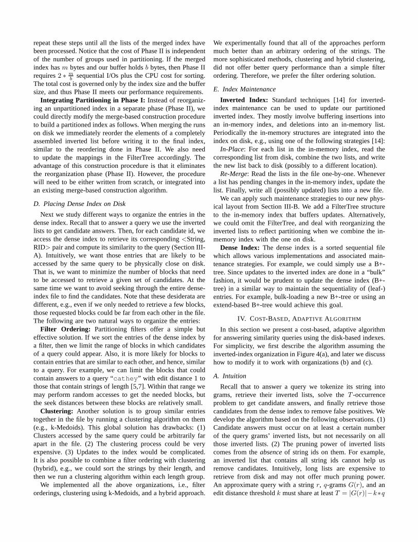
Fig. 4. The inverted list of gram “at” with and without partitioning andpossible mappings to a file on disk. Organization (c) is the best.

Let us examine Figure 4 to discuss possible layouts ofinverted lists partitioned in this fashion. In the left upperportion we see a gramat’s inverted list without partitioning.To the right, the original inverted list is split into differentgroups according to a filter. At the bottom we show possiblestorage layouts. Without partitioning we can simply store thelist contiguously as shown in organization (a). In organization(b), each inverted list is stored contiguously, but the listsbelonging to the same gram from different groups are scatteredacross the file. Finally, organization (c) places the inverted listsbelonging to the same gram contiguously in the file.

Example: Suppose we partitioned the strings by length, asshown in Figure 4. Consider a query with the string “cathey”and an edit-distance thresholdk = 1. Let us examine the costfor retrieving the inverted list of gramat. In organization(a), we perform one disk seek and transfer the five elements1, 2, 3, 4, 5 for at’s inverted list. With filtering, answers tothe query must be within the length range[5, 7], since thelength of the query string “cathey” is six. Therefore, onlythe groups[4, 6) and[6, 8) are relevant. Using organization (b)we transfer three list elements2, 3, 5 with two disk seeks.Note that the elements3, 5 and2 could be arbitrarily farapart in the file. Using organization (c) we transfer the samethree elements2, 3, 5 but with only one disk seek.

C. Constructing Inverted Index on Disk

We now present how to efficiently build an inverted indexin the physical layout shown in Figure 4(c). Since we want toindex large string collections, we cannot assume that the finalindex fits into main memory. Hence, we desire a techniquethat (1) can cope with limited buffer space, and (2) scalesnicely with increasing buffer space. Our main idea is tofirst construct an unpartitioned inverted index with a standardmerge-based method [22] (Phase I), and then reorganize theinverted lists to reflect partitioning (Phase II). This two-phaseapproach has the advantage that any existing constructionprocedure for an inverted index can be directly used in PhaseI, without modification. Later in this subsection, we discussan alternative construction procedure that directly modifies astandard merge-based technique. Figure 5 shows both phasesof index construction, described as follows.

In-Memory

Inverted Lists

1.Tokenize

Runs on Disk

2. Flush

Merged Index

Phase I: Build Index without Filter

Phase II: Reorganize Index

1 2 3 4Merged Index

1, 2, 3, 4, 51.Read

2.Order by

LID, SID

1, 4 3, 5 2

3. Set list addresses

4.Write

3.Merge

[2,4) [4,6) [6,8) [8,10)

FilterTree

SID

1

2

3

4

5

…

String

cat

cathey

kathy

kat

cathy

…

Fig. 5. Two phases of index construction. Phase I builds the index withoutpartitioning. Phase II re-organizes the index to reflect partitioning.

Phase I: This is a standard merge-based construction pro-cedure [22]. We read the strings in the collection one-by-one, decompose them into grams, and add the correspondingstring ids into an in-memory inverted index. Whenever the in-memory index exceeds the buffer limitation, we flush all itsinverted lists with their grams to disk, creating a run. Onceallstrings in the collection have been processed, we combine allruns into the final index in a merge-sort-like fashion.

Phase II: This phase reorganizes the inverted index con-structed in Phase I into a partitioned inverted index bettersuited for approximate string queries. We start with an “empty”FilterTree, whose leaves contain empty mappings from gramsto list addresses. We assign a unique id to each leaf (LID).Then, we sequentially read lists from the merged index untilthe buffer is full. For each of those lists, we re-order itselements based on their FilterTree leaf ids (LID) and stringids (SID). The re-ordering can be supported by a map fromSID to LID created in Phase I, or we can compute the cor-respondingLIDs on-the-fly to save memory. In the process,we set the lengths and offsets (list addresses) for the listsofdifferent groups in the FilterTree. After the elements of eachlist in the buffer have been re-ordered, we write these listsinthe buffer back to disk, in-place, in one sequential write. We

repeat these steps until all the lists of the merged index havebeen processed. Notice that the cost of Phase II is independentof the number of groups used in partitioning. If the mergedindex hasm bytes and our buffer holdsb bytes, then Phase IIrequires2 ∗ m

bsequential I/Os plus the CPU cost for sorting.

The total cost is governed only by the index size and the buffersize, and thus Phase II meets our performance requirements.

Integrating Partitioning in Phase I: Instead of reorganiz-ing an unpartitioned index in a separate phase (Phase II), wecould directly modify the merge-based construction procedureto build a partitioned index as follows. When merging the runson disk we immediately reorder the elements of a completelyassembled inverted list before writing it to the final index,similar to the reordering done in Phase II. We also needto update the mappings in the FilterTree accordingly. Theadvantage of this construction procedure is that it eliminatesthe reorganization phase (Phase II). However, the procedurewill need to be either written from scratch, or integrated intoan existing merge-based construction algorithm.

D. Placing Dense Index on Disk

Next we study different ways to organize the entries in thedense index. Recall that to answer a query we use the invertedlists to get candidate answers. Then, for each candidate id,weaccess the dense index to retrieve its corresponding<String,RID> pair and compute its similarity to the query (Section III-A). Intuitively, we want those entries that are likely to beaccessed by the same query to be physically close on disk.That is, we want to minimize the number of blocks that needto be accessed to retrieve a given set of candidates. At thesame time we want to avoid seeking through the entire dense-index file to find the candidates. Note that these desiderata aredifferent, e.g., even if we only needed to retrieve a few blocks,those requested blocks could be far from each other in the file.The following are two natural ways to organize the entries:

Filter Ordering: Partitioning filters offer a simple buteffective solution. If we sort the entries of the dense indexbya filter, then we limit the range of blocks in which candidatesof a query could appear. Also, it is more likely for blocks tocontain entries that are similar to each other, and hence, similarto a query. For example, we can limit the blocks that couldcontain answers to a query “cathey” with edit distance 1 tothose that contain strings of length [5,7]. Within that range wemay perform random accesses to get the needed blocks, butthe seek distances between these blocks are relatively small.

Clustering: Another solution is to group similar entriestogether in the file by running a clustering algorithm on them(e.g., k-Medoids). This global solution has drawbacks: (1)Clusters accessed by the same query could be arbitrarily farapart in the file. (2) The clustering process could be veryexpensive. (3) Updates to the index would be complicated.It is also possible to combine a filter ordering with clustering(hybrid), e.g., we could sort the strings by their length, andthen we run a clustering algorithm within each length group.

We implemented all the above organizations, i.e., filterorderings, clustering using k-Medoids, and a hybrid approach.

We experimentally found that all of the approaches performmuch better than an arbitrary ordering of the strings. Themore sophisticated methods, clustering and hybrid clustering,did not offer better query performance than a simple filterordering. Therefore, we prefer the filter ordering solution.

E. Index Maintenance

Inverted Index: Standard techniques [14] for inverted-index maintenance can be used to update our partitionedinverted index. They mostly involve buffering insertions intoan in-memory index, and deletions into an in-memory list.Periodically the in-memory structures are integrated intotheindex on disk, e.g., using one of the following strategies [14]:

In-Place: For each list in the in-memory index, read thecorresponding list from disk, combine the two lists, and writethe new list back to disk (possibly to a different location).

Re-Merge: Read the lists in the file one-by-one. Whenevera list has pending changes in the in-memory index, update thelist. Finally, write all (possibly updated) lists into a newfile.

We can apply such maintenance strategies to our new phys-ical layout from Section III-B. We add a FilterTree structureto the in-memory index that buffers updates. Alternatively,we could omit the FilterTree, and deal with reorganizing theinverted lists to reflect partitioning when we combine the in-memory index with the one on disk.

Dense Index: The dense index is a sorted sequential filewhich allows various implementations and associated main-tenance strategies. For example, we could simply use a B+-tree. Since updates to the inverted index are done in a “bulk”fashion, it would be prudent to update the dense index (B+-tree) in a similar way to maintain the sequentiality of (leaf-)entries. For example, bulk-loading a new B+-tree or using anextend-based B+-tree would achieve this goal.

IV. COST-BASED, ADAPTIVE ALGORITHM

In this section we present a cost-based, adaptive algorithmfor answering similarity queries using the disk-based indexes.For simplicity, we first describe the algorithm assuming theinverted-index organization in Figure 4(a), and later we discusshow to modify it to work with organizations (b) and (c).

A. Intuition

Recall that to answer a query we tokenize its string intograms, retrieve their inverted lists, solve theT -occurrenceproblem to get candidate answers, and finally retrieve thosecandidates from the dense index to remove false positives. Wedevelop the algorithm based on the following observations.(1)Candidate answers must occur on at least a certain numberof the query grams’ inverted lists, but not necessarily on allthose inverted lists. (2) The pruning power of inverted listscomes from theabsence of string ids on them. For example,an inverted list that contains all string ids cannot help usremove candidates. Intuitively, long lists are expensive toretrieve from disk and may not offer much pruning power.An approximate query with a stringr, q-gramsG(r), and anedit distance thresholdk must share at leastT = |G(r)|−k∗q

grams with an answer, with|G(r)| = |s| − q + 1. Accordingto the prefix filter (Section II-A), the minimum number oflists we must read to ensure the completeness of answers isminLists = |G(r)| − (T − 1). To understand this equation,consider a string id that occurs onT − 1 lists. To become acandidate, it must additionally occur on at least one of theother|G(r)|− (T − 1) lists. For example, ifq = 2 andk = 1,a query with string “cathey” has |G(r)| = 6 − 2 + 1 = 5grams,T = 5− 1 ∗ 2 = 3 andminLists = 5− (3− 1) = 3.

At one extreme, we could read just theminLists shortestlists. As a consequence, the number of candidates for post-processing could be high, because every string id on thoselists needs to be considered. Recall that for post-processingwe retrieve strings from the dense index (Figure 3), henceevery candidate could require a random disk I/O. At the otherextreme, we could read all the inverted lists for a query,including those long and expensive ones with little pruningpower. It is natural to strive for a solution between the twoextremes, balancing the I/O costs for retrieving inverted listsand for probing the dense index.

B. Algorithm Details

To answer a query we begin by reading theminList

shortest inverted lists (corresponding to grams in the query)from disk into memory. Then we traverse these lists to obtaina set of initial candidates containing all the lists’ stringids(using an algorithm such as “HeapMerge” [18]). The set ofinitial candidates, denoted byC = c1, c2, . . . , c|C|, is a setof triples c = (sid, cnt, cnta). In each triple,sid denotes thestring id of the candidate,cnt denotes the current “count” orthe total number of occurrences ofsid on the lists we have readso far, andcnta denotes the “count absent” value (its meaningwill become clear shortly). Next, we decide whether we canreduce the overall cost of the query by reading additional liststo prune candidates. If so, then we read the next list and prunecandidates with it. If not, then we post-process the candidatesin C. The decision whether or not to read the next list dependson the current number of candidates still inC, the cost forpost-processing them by accessing the dense index, the costfor reading more lists, and the likelihood of pruning candidatesby reading more lists. We repeat this process until we haveread all the query grams’ inverted lists or there is no costreduction from reading additional inverted lists.

Note that the benefits of reading additional inverted listsmight manifest themselves after reading a few more lists, andnot necessarily after reading only one more list. Hence, wemust estimate the effects of reading the nextλ lists. Takeour running example, withr = cathey, k = 1, and lowerboundT = 5 as shown in Figure 6. Let us examine candidatec1 = (2, 2, 2), which is part of the initial candidates producedafter processing theminLists = 3 shortest lists. We haveread 3 of the 5 lists, so there are 2 lists left. In order to prunecandidatec1, its string id must be absent on at leastcnta = 2additional lists.

In general, the “count absent” value is the minimum numberof additional lists a candidate string id must beabsent from,

Inverted Lists for Query s=cathey, k=1, q=2, T=3

minLists = 3

Initial Candidates

c1 = (2, 2, 2)

c2 = (1, 1, 1)

c3 = (3, 1, 1)

c4 = (5, 1, 1)

ca

1

2

5

th

1

3

5

at

1

2

3

4

5

ey

2

hy

2

Fig. 6. Example to illustrate meaning and effect of the “count absent” value.

in order to be pruned. At each stage in the adaptive algorithmfor answering a query with stringr and q-gramsG(r), wecan compute the count-absent value of a triple(sid, cnt, cnta)corresponding to a candidate answer by:

cnta = (|G(r)| −minLists)− (T − cnt) + 1. (1)

Candidates could have variouscnta values, and the cost andbenefit of reading more lists depend onλ, i.e., the numberof additional lists we consider reading. Since the benefits ofreading more lists can become apparent only after readingseveral next lists, a cost model that considers only readingthenext list could get stuck in a local minimum, and is thereforeinsufficient to find a globally minimal cost. This is the reasonwhy we need to consider reading all the possible numbers ofremaining listsλ. For example, in the first iteration we wouldconsider1 ≤ λ ≤ |G(r)| −minLists.

Pseudo-Code:Figure 7 shows pseudo-code for the adaptivealgorithm. We useΩ(r) to denote the list addresses sortedby length in an increasing order for a query stringr. Forconvenience we useΩ(r)[j] to mean thej-th list in Ω(r).Cλ refers to the subset of candidates withcnta ≤ λ. Weassume the following parameters of a cost-model: (1)Θ is theaverage cost of post-processing a candidate, (2)Π(l) is thecost of reading listl, and (3)ben(λ) is the benefit or readingλ additional lists.

Input: Inverted list addressesΩ(r) for a query stringrMinimum number of lists to readminLists

Output: A setC of candidate answers to be post-processedMethod:1. C = HeapMerge(Ω(r), minLists);2. nextList = minLists + 1;3. listsLeft = |Ω(r)| −minLists;4. WHILE listsLeft > 05. FOR λ = 1 TO listsLeft6. Λ = nextλ lists starting fromΩ(r)[nextList];7. costPP =|Cλ| ∗Θ; // cost of post-processing8. costRL =

∑l∈Λ

Π(l); // cost of reading lists9. benfitRL =ben(λ) for lists in Λ;10. IF (costRL - benefitRL< costPP)THEN11. invList = readList(Ω(r)[nextList]);12. C = pruneCandidates(C, invList);13. nextList+=1; listsLeft−=1;14. BREAK FOR;15. END IF16. END FOR17. IF λ == listsLeft THEN BREAK WHILE; // no benefit18. END WHILE19. RETURN C;

Fig. 7. Cost-based, adaptive algorithm for answering queries.

We begin by readingminLists inverted lists and processthem to obtain a set of initial candidates (line 1). Next,we consider reading all numbers of remaining lists, settingλ accordingly. We compute the cost of post-processing thecandidates that could potentially be pruned withλ lists (line7). Correspondingly, we compute the cost (line 8) and benefit(line 9) of reading the nextλ lists. We decide whether we canreduce the overall cost by readingλ lists, as compared to notreading them (line 10). If we can reduce the cost, we read thenext list (line 11) and prune candidates (line 12). Otherwise,we proceed with the nextλ. We repeat this process until (a)we have read all lists or (b) we cannot benefit from readingany more lists. Notice that whenever we detect a benefit weread justone more list at a time, independent of the valueof λ. This approach mitigates possible inaccuracies of a realcost-model.

C. Cost Model

In this section we develop a model to estimate the cost andbenefit of reading additional inverted list.

Cost of post-processing candidates: We focus on the I/Ocost because the CPU time for computing similarities is oftennegligible in comparison. The maximum cost for retrieving acandidate string is the time for one disk seek plus the time totransfer one disk block. This cost can be determined directlyfrom the hardware configuration or estimated offline. We canimprove this model by taking into account the chance thata dense index block is already cached in memory. Using aconservative but simple approach, we read a few blocks offlineand compute the average time to retrieve a block, denoted byΘ. We then use|C|∗Θ to estimate the cost of post-processinga candidate setC. For example, the cost of post-processingthe candidates in Figure 6 would be 4*Θ since|C| = 4.

Cost of retrieving inverted lists: Since the lengths ofinverted lists usually follow a Zipf distribution, the averageretrieval time is not an accurate estimator of the true cost.Again, the cost is determined by the seek time and the transferrate of the disk. Since our solution is on top of a file system,the raw disk parameters are not very accurate performanceindicators either, due to the intermediate layer. To overcomethis issue, we read a few lists offline and do a linear regressionto obtain the cost functionΠ(ω) = m ∗ ω.l + b, whereω.ldenotes the length of the inverted listω, b is an estimate forthe seek time, andm is an estimate for the inverse transferrate. So, given a setΩ of ω, we can estimate the total cost ofreading all those inverted lists by

∑

ω∈ΩΠ(ω). For example,the cost of reading the lists of gramsca andat from Figure 6would be(m ∗ 3 + b) + (m ∗ 5 + b), since their lengths are 3and 5, respectively.

Benefit of reading additional inverted lists: At a highlevel, we quantify the benefit in terms of the cost we cansave by pruning candidates, considering the likelihood of thathappening by readingλ lists. The likelihood of pruning acandidatec with λ lists depends on itscnta. Intuitively, wewould like to know the probability thatc’s string id is absentfrom at leastcnta of the λ lists. Computing this probability

for each candidate individually would be computationallyexpensive. To avoid repeated computations we group thecandidates bycnta as follows. We define a subset ofC asC(i) = c|c ∈ C ∧ c.cnta = i, containing all candidates inC that have a certaincnta = i. We also make the followingsimplifying assumptions:• The probability of one string id being present or absent

from an inverted list is independent of the presence orabsence of another string id on the same list.

• The probability of a string id being present or absent fromone inverted list is independent of that same string id beingabsent or present from another list.

Following these assumptions, we estimate the benefit as:

ben(λ) = Θ ∗

λ∑

i=1

|C(i)| ∗ p(i, λ), (2)

wherep(i, λ) denotes the probability of a string id being absentfrom i of the λ lists. In a sense, we are being optimistic,since Equation 2 expresses that we could pruneall candidatesin C(i) with probability p(i, λ). The key challenge is toobtain a reasonably accuratep(i, λ) efficiently. Following ourassumptions we modelp(i, λ) as a sequence ofλ independentBernoulli trials, i.e., a Bernoulli process. We define “success”as the absence of a string id on a list, and “failure” as thepresence of a string id on a list. Since all we know of the listsare their lengths, we estimate the success probability withasetΩ of list addressesω as:

ps = 1−

∑

ω∈Ω ω.l

|Ω|∗

1

N. (3)

The term∑

ω∈Ωω.l

|Ω| denotes the average list length of theλ listsin Ω we are considering to read, andN is the total numberof strings in the dense index. The probability of at leasti

successes inλ trials having a success probabilityps can becomputed with the cumulative binomial distribution function:

p(i, λ) = binom(i, λ, ps) =

λ∑

j=i

(

λ

j

)

pjs(1− ps)λ−j . (4)

Combining Equations 2, 3 and 4 yields a complete model forestimating the benefit of readingλ additional lists:

ben(λ) = Θ ∗

λ∑

i=1

|C(i)| ∗ binom(i, λ, ps). (5)

D. Combining with Partitioned Inverted-Index Layout

So far, we have presented the adaptive algorithm using thelayout in Figure 4(a) from Section III for simplicity. Next,we discuss how to combine the adaptive algorithm with theother two inverted-index layouts (b) and (c). Recall that whenanswering a query we first traverse the FilterTree to identifythe relevant groups (e.g., corresponding to length ranges)which could contain answers.

Modified Success Probability: In Equation 3 the proba-bility (called success probability) of a string id being absentfrom a set of lists depends on their average list length, and

the total number of stringsN in the dataset. Since each groupgenerated by a partitioning filter only contains a subset of theN total strings, simply applying Equation 3 would lead tooverestimation of the success probability, and consequentlyoverestimation of the benefit (Equation 5). We modify thesuccess probability by replacingN in Equation 3 with thenumber of strings in the particular group we are considering.This change applies to both inverted-index layouts (b) and (c).Next, we detail how to answer queries with those two layouts.

Layout (b): To answer a query using the adaptive algorithm,we first identify all relevant groups, and then process eachgroup individually as if there was no partitioning (but withthenew success probability). Each instance of the algorithm triesto minimize the cost for processing its corresponding group.

Layout (c): Intuitively, we just process all relevant groupstogether, as opposed to processing them one-by-one. We firstread theminList inverted lists of all relevant groups to createthe sets of initial candidates forall groups at the same time.To exploit the contiguous layout, we retrieve the lists grambygram. That is, we read the lists of all relevant groups of thefirst gram, then we read the lists of all relevant groups of thesecond gram, etc., until we have retrieved all theminLists

lists. We perform HeapMerge on the groups separately to getthe initial sets of candidates.

Next, we proceed with the iterative phase of the algorithm,estimating the cost and benefit of reading the next grams’ listsof all relevant groups. We either decide to read the next liststogether or commence post-processing.

Layout (c) Examples: In the following, we describe how tohandle a few interesting scenarios when combining the adap-tive algorithm with organization (c). For example, Figure 8shows the inverted lists of the relevant groups for our runningexamplecathey (the string ids differ from earlier examples).To minimize the global cost we should read the lists for gramhy first because there are a total of 3 relevant elements2, 6,8. Next, we should read the lists of gramey because theycontain a total of 4 elements2, 6, 7, 8, and so on.

Local vs. Global Ordering: We want to read the invertedlists from shortest to longest. However, the local order of eachgroup may not correspond to the best global order. We mustread the relevant lists of grams in order of their sum of lengths.

ca

1

2

5

th

1

3

5

at

1

2

3

4

5

ey

2

hy

2

ca

6

7

8

9

th

8

9

at

6

ey

6

7

8

hy

6

8

Group [4,6) Group [6,8)

Fig. 8. Inverted lists for querycathey, k = 1, q = 2, andT = 3.

Pruning Entire Groups: Groups that do not contain at leastT grams of the query can be pruned entirely. We should notread the lists that do match a query’s grams of a pruned group.

Figure 9 shows a group [6,8) that has less thanT of thequery’s grams. Since this group cannot contain answers to thequery, we do not need to read lists from it. For example, forgramca that exists in group [6,8), we should only read theelements1,2,5 andnot the elements6,7,8,9.

A similar situation can arise during the iterative phase ofthe adaptive algorithm. When a particular group does notcontribute candidates anymore (because they have all beenpruned), then we do not need to read inverted lists fromthat group anymore (but possibly still from the other ones).We must handle both scenarios above specially during costestimation and during the retrieval of lists.

ca

1

2

5

th

1

3

5

at

1

2

3

4

5

ey

2

hy

2

ca

6

7

8

9

that ey

6

7

8

hy

Group [4,6) Group [6,8)

Fig. 9. Inverted lists for querycathey, k = 1, q = 2, andT = 3. Noneof the strings in group [6,8) contain the gramsat, th, or ty.

V. EXPERIMENTS

In this section, we evaluate the performance of queries andindex construction of our techniques. We show experiments onrange and top-k queries using edit distance, and range queriesusing normalized edit distance, Jaccard based onq-grams, andJaccard based on word grams. We compare our techniques toa recent tree-based index BED-tree [21], whenever possible.

Datasets:We used six real datasets, summarized in Table I.The first four datasets are taken from [21] (BED-tree) toestablish a fair comparison. In addition, we used the last twodatasets for experiments on scalability and index-constructionsince they are larger than the first four.

Dataset # Strings Max Len Avg LenDBLP Author 2,948,929 48 15DBLP Title 1,158,648 667 68IMDB Actor 1,213,391 73 16

Uniprot 508,038 1992 341

Medline Titles 10,000,000 252 84Web Word Grams 20,000,000 163 23

TABLE I

DATASETS AND THEIR STATISTICS.

The DBLP Title and Author datasets1 were taken fromDBLP, and contained authors and titles of publications. TheIMDB Actor2 dataset consists of actor names from movies.The Uniprot3 dataset contains protein sequences in text format.The Medline Titles4 dataset consists of publication titlesfrom the medical domain. Finally, the Web Word Grams5

dataset contains popular word-grams from web documents. Werandomly picked 10 million titles of the Medline Dataset, and20 million 4-word-grams for the Web Word Grams dataset.

Hardware and Compiler: We conducted all experimentson a machine with a four-core Intel Xeon E5520 2.26Ghzprocessor, 12GB of RAM, and a 10,000 RPM disk drive,running a Ubuntu operating system. We used the original codefor BED-tree written in C++ which the authors generously

1www.informatik.uni-trier.de/˜ley/db2www.imdb.com3www.uniprot.org4www.ncbi.nlm.nih.gov/pubmed5www.ldc.upenn.edu/Catalog, number LDC2006T13

provided to us. We implemented all our algorithms in C++ aswell. We compiled all code with GCC using the “-O3” flag.

Parameters:We experimented with differentq for tokeniz-ing strings intoq-grams and foundq = 3 to be best for mostcases. Therefore, we usedq = 3 for all experiments, for bothBED-tree (where applicable) and for out techniques. For ourtechniques, we used the length filter for partitioning. We useda disk-block size of 8KB for both BED-tree and our methods.

Clearing Filesystem Cache:In our experiments we con-sidered both the raw disk performance of queries, and theirperformance with caching. To simplify the implementations,both BED-tree and our techniques were built on top of afilesystem (as opposed to using the raw disk device). Usinga filesystem, however, complicates accurate measurements ofdisk performance due to filesystem caching (it will aggres-sively use all available memory to cache disk pages). Toovercome this issue, we cleared the filsystem cache at certainpoints (to be explained) with the following shell command:

echo 3 > /proc/sys/vm/drop_caches

Query Workloads: The authors of the BED-tree providedus with the data and workloads from their experiments in [21].The workload for each dataset consisted of 100 randomlychosen strings. For the other datasets used only in this pa-per (Medline Titles, Web Word Grams), we also generatedworkloads by randomly choosing 100 strings for each dataset.

A. Index Construction Performance

We built inverted indexes for the Web Word Grams datasetsin organization (c) (Section III) using length filtering. Wemeasured each step of the construction procedure (1) creatingruns, (2) merging the runs, and (3) reorganizing the index,clearing the filesystem cache before each step. We also ranthis experiment on the Medline Titles dataset, but omit theresults since they show a similar trend.

0

1

2

3

4

5

6

7

4 8 12 16 20Con

stru

ctio

n T

ime

(min

s)

Number of Strings (millions)

Create Runs (Phase I)Merge Runs (Phase I)

Reorganize Index (Phase II)

0

2

4

6

8

10

12

14

50 100 150 200Con

stru

ctio

n T

ime

(min

s)

Buffer Size (MB)

Create Runs (Phase I)Merge Runs (Phase I)

Reorganize Index (Phase II)

Fig. 10. Index construction performance on Web Word Grams.

In the left chart of Figure 10 we allocated a fixed buffersize of 400MB for index construction. It shows that the index-construction procedure scaled well (almost linearly) withthesize of the dataset. The right chart shows the constructionperformance with varying buffer sizes, and we see that themerging of the runs took most of the time. By increasingthe buffer size we improved the performance of merging theruns. The other two phases, creating the runs and reorganizingthe index, did not benefit from a larger buffer size becausethey were CPU bound, explained as follows. Creating the runsconsists of tokenizing the strings, and frequently reallocating

in-memory inverted lists. Reorganizing the index consistsofsorting inverted-list elements, while performing disk opera-tions in buffer-sized chunks.

We do not report the construction times for BED-tree forthe following reason. A comparison would be somewhat unfairsince our technique builds its inverted index in “bulk”, whileBED-tree does not currently implement bulk-loading (it usesrepeated insertions). For example, constructing a BED-tree on20 million Web Word Grams with a 100MB buffer took around9 hours, and still almost 4 hours with a 400MB buffer.

B. Query Performance Naming Conventions and Methodology

In this subsection, we introduce the different flavors ofBED-tree and the inverted-index approach used in our exper-iments on query performance. We also detail our proceduresfor obtaining the results of different types of experiments.

BED-Tree Naming: We follow the convention from [21].BD, BGC, and BGL refer to a BED-tree using the dictionaryorder, gram count order, and gram location order, respectively.

Naming of Our Approaches: In our experiments wefocused on the following two extreme approaches showingthe best and worst inverted-index solutions for raw diskperformance. “Simple” refers to a straightforward adoption ofexisting algorithms. It uses an unpartitioned inverted indexand a dense index whose entries are in an arbitrary order.“Simple” retrieves all the inverted lists of a query string’sgrams and then solves theT -occurrence problem with anefficient in-memory algorithm (we used DivideSkip [15]). Weuse “AdaptPtOrd” to refer to our most advanced method usingthe adaptive algorithm (“Adapt”), a partitioned inverted index(“Pt”), and a dense index with entries ordered by their length(“Ord”). More results exploring the various dimensions of oursolutions can be found in the full paper [6].

Raw Disk: In this type of experiments, we measured theperformance of queries when all data required for answeringa query (inverted lists, dense index blocks, BED-tree blocks)needed to be retrieved from disk. To do so, we cleared thefilesystem cache before each query. Recall that our inverted-index assumes the FilterTree is in memory (Section III-A). Fora fair comparison, we allocated the same amount of memoryneeded for the FilterTree to BED-tree’s buffer manager. Notethat BED-tree implements its own buffer manager, and there-fore, those blocks cached in its buffer manager were unaffectedby clearing the filesystem cache.

We also gathered the number of disk seeks and the amountof data transferred from disk per query captioned as ”DataTransferred” and “Disk Seeks”. For BED-tree the disk seeksare the number of nodes retrieved from disk (not already in thebuffer manager), and the data transferred is that number mul-tiplied by the block size. For our inverted-index solution,thenumber of disk seeks is the number of inverted lists and dense-index blocks accessed. We computed the data transferred usingthe sizes of the inverted lists and dense-index blocks.

Fully Cached Index: This experiment represents the otherextreme in which all data required to answer a query isalready in memory. For BED-tree we achieved this behavior

by allocating a large amount of memory in its buffer manager.We ran our workloads immediately after building the BED-tree, and therefore, the entire BED-tree was in memory whenrunning queries. For our inverted-index approach we reliedon the filesystem for caching. We first built the invertedindex and dense index without clearing the filesystem cache,and then immediately ran our workloads, assuming that afterconstruction all indexes are probably in the filesystem’s cache.

C. Range Queries Using Edit Distance

0.1

1

10

100

1 2 3 4Avg

Que

ry T

ime

(s)

Edit Distance

BDBGCBGL

SimpleAdaptPtOrd

(a) Raw Disk Time.

1

10

100

1000

1 2 3 4Avg

Que

ry T

ime

(ms)

Edit Distance

BDBGCBGL

SimpleAdaptPtOrd

(b) Fully Cached Index Time.

0.1

1

10

100

1000

1 2 3 4Dat

a T

rans

ferr

ed (

MB

)

Edit Distance

BDBGCBGL

SimpleAdaptPtOrd

(c) Data Transferred.

0.1

1

10

100

1000

1 2 3 4Dis

k S

eeks

(x1

00)

Edit Distance

BDBGCBGL

SimpleAdaptPtOrd

(d) Disk Seeks.

Fig. 11. Range-query performance on DBLP Author.

0.01

0.1

1

10

100

1 2 4 8 16Avg

Que

ry T

ime

(s)

Edit Distance

BDBGCBGL

SimpleAdaptPtOrd

(a) Raw Disk Time.

0.1

1

10

100

1000

1 2 4 8 16Avg

Que

ry T

ime

(ms)

Edit Distance

BDBGCBGL

SimpleAdaptPtOrd

(b) Fully Cached Index Time.

0.01

0.1

1

10

100

1000

1 2 4 8 16Dat

a T

rans

ferr

ed (

MB

)

Edit Distance

BDBGCBGL

SimpleAdaptPtOrd

(c) Data Transferred.

0.1

1

10

100

1000

1 2 4 8 16Dis

k S

eeks

(x1

00)

Edit Distance

BDBGCBGL

SimpleAdaptPtOrd

(d) Disk Seeks.

Fig. 12. Range-query performance on DBLP Title.

1) Comparison with BED-Tree: Next, we compare ourapproach with BED-tree on range-query performance usingthe datasets and workloads from the BED-tree paper [21]. Thefirst two graphs, (a) and (b), of Figures 11-14 show the rawdisk, and fully cached index times, respectively. The graphs(c) and (d) further detail the raw disk performance with theaverage number of disk seeks and data transferred per query.

0.01

0.1

1

10

100

1 2 3 4Avg

Que

ry T

ime

(s)

Edit Distance

BDBGCBGL

SimpleAdaptPtOrd

(a) Raw Disk Time.

0.1

1

10

100

1000

1 2 3 4Avg

Que

ry T

ime

(ms)

Edit Distance

BDBGCBGL

SimpleAdaptPtOrd

(b) Fully Cached Index Time.

0.1

1

10

100

1000

1 2 3 4Dat

a T

rans

ferr

ed (

MB

)

Edit Distance

BDBGCBGL

SimpleAdaptPtOrd

(c) Data Transferred.

0.1

1

10

100

1000

1 2 3 4Dis

k S

eeks

(x1

00)

Edit Distance

BDBGCBGL

SimpleAdaptPtOrd

(d) Disk Seeks.

Fig. 13. Range-query performance on IMDB Author.

0.01

0.1

1

10

100

1 2 4 8 16Avg

Que

ry T

ime

(s)

Edit Distance

BDBGCBGL

SimpleAdaptPtOrd

(a) Raw Disk Time.

0.1

1

10

100

1000

10000

1 2 4 8 16Avg

Que

ry T

ime

(ms)

Edit Distance

BDBGCBGL

SimpleAdaptPtOrd

(b) Fully Cached Index Time.

0.01 0.1

1 10

100 1000

10000

1 2 4 8 16Dat

a T

rans

ferr

ed (

MB

)

Edit Distance

BDBGCBGL

SimpleAdaptPtOrd

(c) Data Transferred.

0.1

1

10

100

1000

10000

1 2 4 8 16Dis

k S

eeks

(x1

00)

Edit Distance

BDBGCBGL

SimpleAdaptPtOrd

(d) Disk Seeks.

Fig. 14. Range-query performance on Uniprot.

We see that “AdaptPtOrd” consistently outperformed BED-treeby orders of magnitude, both for raw disk peformance andfor a fully cached index (notice we are using a log scale onthe y-axes). Also, “AdaptPtOrd” was considerably faster than“Simple”. The performance differences between “AdaptPtOrd”and the BED-tree variants on raw disk are explained by thegraphs (c) and (d). “AdaptPtOrd” transferred significantlylessdata per query with fewer disk seeks than BED-tree. Thetwo main reasons why BED-tree examined so many nodesare as follows. First, the pruning power at higher levels ofthe BED-tree is weak because a node entry refers to theenclosing interval of ranges in its subtree. Second, the BED-tree search procedure traverse multiple paths in the tree (moreakin to an R-tree search), leading to additional node accessesas compared to a standard B-tree range search. Such a searchprocedure can also incur long disk-seek distances, becauseit isimpossible to simultaneously store all tree-nodes close toeachother (in a standard B-tree we only need to store the leavesclose to their siblings). Our argument that BED-tree’s pruning

power is not as strong as our approach is also supported bythe results on fully cached indexes, where a significant costiscomputing the real edit distances to candidate answers.

In Table II we summarized the index sizes for these sets ofexperiments. We observe that, in general, our inverted indexapproach requires more space than BED-tree. For example,on DBLP Author the BED-tree with dictionary ordering (BD)required 97MB of disk-space, and our indexes required 82 +204 = 292MB on disk. However, our approaches transferredmuch less data from disk per query (see Figures 11-14). Also,recall that for the raw disk experiments, we give the BED-treevariants a buffer space equal to “FT”, the size of our FilterTree.

Dataset BD BGC BGL DenIx InvIx FTDBLP Author 97 225 189 82 204 7DBLP Title 123 156 157 100 297 21IMDB Actor 38 88 75 32 88 11

Uniprot 283 302 305 222 617 49

TABLE II

INDEX SIZES IN MB OF BED-TREE VARIANTS AND OUR INVERTED-INDEX

COMPONENTS. DENIX REFERS TO THE DENSE INDEX, INV IX TO THE

INVERTED INDEX, AND FT TO THE IN-MEMORY FILTERTREE.

2) Scalability: In Figures 15 and 16 we varied the numberof indexed strings on our two large datasets, Web WordGrams and Medline Titles, to evaluate the scalability of ourtechniques. Due to its slow performance we omit BED-treefrom the raw disk experiments. For example, on 12 millionWeb Word Grams its best version BD needed an average of15 seconds per query, and on 6 million Medline Titles its bestversion BGC needed an average of 145 seconds. Similarly,we only plot the best version of BED-tree for the in-memoryresults since the other versions were significantly worse.

Our results show that “AdaptPtOrd” offers better scalabilitythan “Simple”, explained as follows. As we increased the sizeof the dataset, some inverted lists became longer. However,the number of results per query grew relatively slower thanthe total index size. Especially for highly selective queries, theadaptive algorithm avoided reading many unnecessary invertedlists. This effect explains the excellent performance on thehighly selective Medline Titles. Similar arguments hold forthe experiments with fully cached indexes.

0

0.2

0.4

0.6

0.8

1

4 8 12 16 20

Avg

Que

ry T

ime

(s)

Number of Strings (millions)

Simple AdaptPtOrd

(a) Raw Disk Time.

0 20 40 60 80

100 120 140

4 8 12 16 20Avg

Que

ry T

ime

(ms)

Number of Strings (millions)

BDSimple

AdaptPtOrd

(b) Fully Cached Index Time.

Fig. 15. Range-query scalability with edit distance 2 on WebWord Grams.

D. Top-K Queries Using Edit Distance

Next, we discuss our results on top-k queries shown inFigures 17 and 18. As before we used the datasets and

0

1

2

3

4

5

2 4 6 8 10

Avg

Que

ry T

ime

(s)

Number of Strings (millions)

Simple AdaptPtOrd

(a) Raw Disk Time.

0

100

200

300

400

500

600

2 4 6 8 10Avg

Que

ry T

ime

(ms)

Number of Strings (millions)

BGCSimple

AdaptPtOrd

(b) Fully Cached Index Time.

Fig. 16. Range-query scalability with edit distance 6 on Medline Title.

workloads of the BED-tree paper. We answer top-k querieson our inverted-index by a sequence of range queries withincreasing ranges. We do not show the results on the DBLPTitle and Uniprot datasets, because for some queries BED-treedid not find all correct answers. For example, on Uniprot withK=4, BED-tree only returned a total of 304 answers insteadof the correct 400 answers for the 100 queries.

The results on top-k queries are consistent with those onrange queries, and similarity show our techniques answeredtop-k queries efficiently, and outperformed BED-tree.

0.01

0.1

1

10

100

1 2 4 8 16Avg

Que

ry T

ime

(s)

K

BDBGCBGL

SimpleAdaptPtOrd

(a) Raw Disk Time.

0.1

1

10

100

1000

1 2 4 8 16Avg

Que

ry T

ime

(ms)

K

BDBGCBGL

SimpleAdaptPtOrd

(b) Fully Cached Index Time.

Fig. 17. Top-K query performance on DBLP Author.

0.01

0.1

1

10

100

1 2 4 8 16Avg

Que

ry T

ime

(s)

K

BDBGCBGL

SimpleAdaptPtOrd

(a) Raw Disk Time.

0.1

1

10

100

1000

1 2 4 8 16Avg

Que

ry T

ime

(ms)

K

BDBGCBGL

SimpleAdaptPtOrd

(b) Fully Cached Index Time.

Fig. 18. Top-K query performance on IMDB Actor.

E. Query Performance Using Other Similarity Functions

In this subsection, we present experiments on range queriesusing normalized edit distance and Jaccard. Its main purposeis to demonstrate that our solutions also support similarityfunctions other than edit distance. Due to space limitations,we omit some of the figures since they are consistent with theoverall trends. The complete set of experimental results canbe found in the full version of this paper [6].

1) Normalized Edit Distance: Again, we used the datasetsand workloads from the BED-tree paper. Since BED-treecurrently supports normalized edit distance only with the gramcounting order, we have only BGC in Figures 19 and 20. Asbefore, “AdaptPtOrd” outperforms its competitors.

0.01

0.1

1

10

100

0.8 0.85 0.9 0.95

Avg

Que

ry T

ime

(s)

Normalized Edit Distance

BGCSimple

AdaptPtOrd

(a) Raw Disk Time.

1

10

100

1000

0.8 0.85 0.9 0.95Avg

Que

ry T

ime

(ms)

Normalized Edit Distance

BGCSimple

AdaptPtOrd

(b) Fully Cached Index Time.

Fig. 19. Range-query performance on DBLP Author.

0.1

1

10

100

0.8 0.85 0.9 0.95

Avg

Que

ry T

ime

(s)

Normalized Edit Distance

BGCSimple

AdaptPtOrd

(a) Raw Disk Time.

1

10

100

1000

0.8 0.85 0.9 0.95Avg

Que

ry T

ime

(ms)

Normalized Edit Distance

BGCSimple

AdaptPtOrd

(b) Fully Cached Index Time.

Fig. 20. Range-query performance on DBLP Title.

2) Jaccard with Q-Gram Tokens: In Figure 21 we used theJaccard similarity of multisets ofq-gram tokens to quantify thesimilarity between strings. Though BED-tree could possiblyanswer queries using Jaccard with the gram count ordering, itscurrent implementation does not support it. Therefore, we onlyplot the results of our approaches. We observe that our newtechniques also provide a disk-performance benefit to queriesusing Jaccard.

0

0.1

0.2

0.3

0.4

0.5

0.6

0.9 0.8 0.7 0.6

Avg

Que

ry T

ime

(s)

Jaccard

Simple AdaptPtOrd

(a) DBLP Author.

0

0.2

0.4

0.6

0.8

1

1.2

0.9 0.8 0.7 0.6

Avg

Que

ry T

ime

(s)

Jaccard

Simple AdaptPtOrd

(b) DBLP Title.

Fig. 21. Raw disk range-query performance using Jaccard onq-gram tokens.

3) Jaccard with Word Tokens: For those datasets with verylong strings (DBLP Title, Medline Title), it could be moremeaningful to use Jaccard based on word tokens to quantifythe similarity between strings. Figure 22 shows the raw diskperformance of queries based on word tokens, and we see thatour techniques also improved their performance in this setting.

0

0.1

0.2

0.3

0.4

0.9 0.8 0.7 0.6

Avg

Que

ry T

ime

(s)

Jaccard

Simple AdaptPtOrd

(a) DBLP Title.

0

1

2

3

0.9 0.8 0.7 0.6

Avg

Que

ry T

ime

(s)

Jaccard

Simple AdaptPtOrd

(b) Medline Title.

Fig. 22. Raw disk range-query performance using Jaccard on word tokens.

VI. CONCLUSION

We have studied approximate string selection queries whendata and indexes reside on disk. We proposed a new physicallayout for an inverted index, demonstrated how to efficientlyconstruct it, and showed its benefits to query processing. Wedeveloped a cost-based adaptive algorithm to answer queries.We have shown that the adaptive algorithm and the new indexlayout complement each other and that their combination an-swers queries efficiently. Further, our techniques outperformeda recent tree-based index, BED-tree.

Acknowledgements: This work was supported by the CluE(IIS 0844574) and Asterix (IIS 0910989) NSF grants, and theNational Nature Science of China grant number 60828004.

REFERENCES

[1] Oracle Text, An Oracle Technical White Paper, 2007. http://www.oracle.com/technology/products/text/pdf/11goracletexttwp.pdf.

[2] Fuzzy Search in IBM DB2 9.5, 2008. http://publib.boulder.ibm.com/infocenter/db2luw/v9r5/index.jsp?topic=/com.ibm.db2.luw.admin.nse.topics.doc/doc/t0052178.html.

[3] A. Arasu, V. Ganti, and R. Kaushik. Efficient exact set-similarity joins.In VLDB, pages 918–929, 2006.

[4] R. J. Bayardo, Y. Ma, and R. Srikant. Scaling up all pairs similaritysearch. InWWW, 2007.

[5] A. Behm, S. Ji, C. Li, and J. Lu. Space-constrained gram-based indexingfor efficient approximate string search. InICDE, 2009.

[6] A. Behm, C. Li, and M. J. Carey. Answering approximate string querieson large datasets using external memory (full version). Technical report,Department of Computer Science, UC Irvine, July 2010.

[7] S. Buettcher and C. L. A. Clarke. Index compression is good, especiallyfor random access. InCIKM, 2007.

[8] S. Chaudhuri, K. Ganjam, V. Ganti, R. Kapoor, V. Narasayya, andT. Vassilakis. Data cleaning in Microsoft SQL Server 2005. In SIGMOD,2005.

[9] S. Chaudhuri, V. Ganti, and R. Kaushik. A primitive operator forsimilarity joins in data cleaning. InICDE, 2006.

[10] L. Gravano, P. G. Ipeirotis, H. V. Jagadish, N. Koudas, S. Muthukrishnan,and D. Srivastava. Approximate string joins in a database (almost) forfree. In VLDB, pages 491–500, 2001.

[11] M. Hadjieleftheriou, A. Chandel, N. Koudas, and D. Srivastava. Fastindexes and algorithms for set similarity selection queries. In ICDE,2008.

[12] E. Hunt, M. P. Atkinson, and R. W. Irving. A database index to largebiological sequences. InIn VLDB, pages 139–148, 2001.

[13] Y. Kim, K.-G. Woo, H. Park, and K. Shim. Efficient processing ofsubstring match queries with inverted q-gram indexes. InICDE, 2010.

[14] N. Lester, J. Zobel, and H. Williams. Efficient online index maintenancefor contiguous inverted lists.Inf. Process. Manage., 42(4), 2006.

[15] C. Li, J. Lu, and Y. Lu. Efficient merging and filtering algorithms forapproximate string searches. InICDE, pages 257–266, 2008.

[16] C. Meek, J. M. Patel, and S. Kasetty. Oasis: An online andaccuratetechnique for local-alignment searches on biological sequences, 2003.

[17] G. Navarro. A guided tour to approximate string matching. ACMComput. Surv., 33(1):31–88, 2001.

[18] S. Sarawagi and A. Kirpal. Efficient set joins on similarity predicates.In SIGMOD Conference, 2004.

[19] E. Ukkonen. Approximae string matching with q-grams and maximalmatching.Theor. Comut. Sci., 1:191–211, 1992.

[20] C. Xiao, W. Wang, and X. Lin. Ed-join: An efficient algorithm forsimilarity joins with edit distance constraints. InVLDB, 2008.

[21] Z. Zhang, M. Hadjieleftheriou, B. C. Ooi, and D. Srivastava. Bed-tree:an all-purpose index structure for string similarity search based on editdistance. InSIGMOD, 2010.

[22] J. Zobel and A. Moffat. Inverted files for text search engines. ACMComput. Surv., 38(2):6, 2006.

[23] M. Zukowski, S. Heman, N. Nes, and P. Boncz. Super-scalar RAM-CPUcache compression. 2006.