ansys cfx tutorial laminar flow in a rectangular...

ANSYS CFX Tutorial Laminar Flow in a Rectangular Duct 2019-09-10 V5.00

University of Manitoba of 25

ANSYS CFX Tutorial

Laminar Flow in a Rectangular Duct

Scott J. Ormiston Jeffrey R. Berg

Department of Mechanical Engineering

University of Manitoba

Winnipeg, Manitoba Canada

V5.00

2019-09-10



1. Introduction This tutorial has been adapted from a basic tutorial that was originally developed for CFX-TASCflow. It has been adapted for ANSYS CFX and now uses a mesh created by ANSYS Meshing in ANSYS Workbench. The objective of this tutorial is to help a new user of CFX to progress through the basic steps of setting up and running an isothermal single phase laminar internal flow simulation.

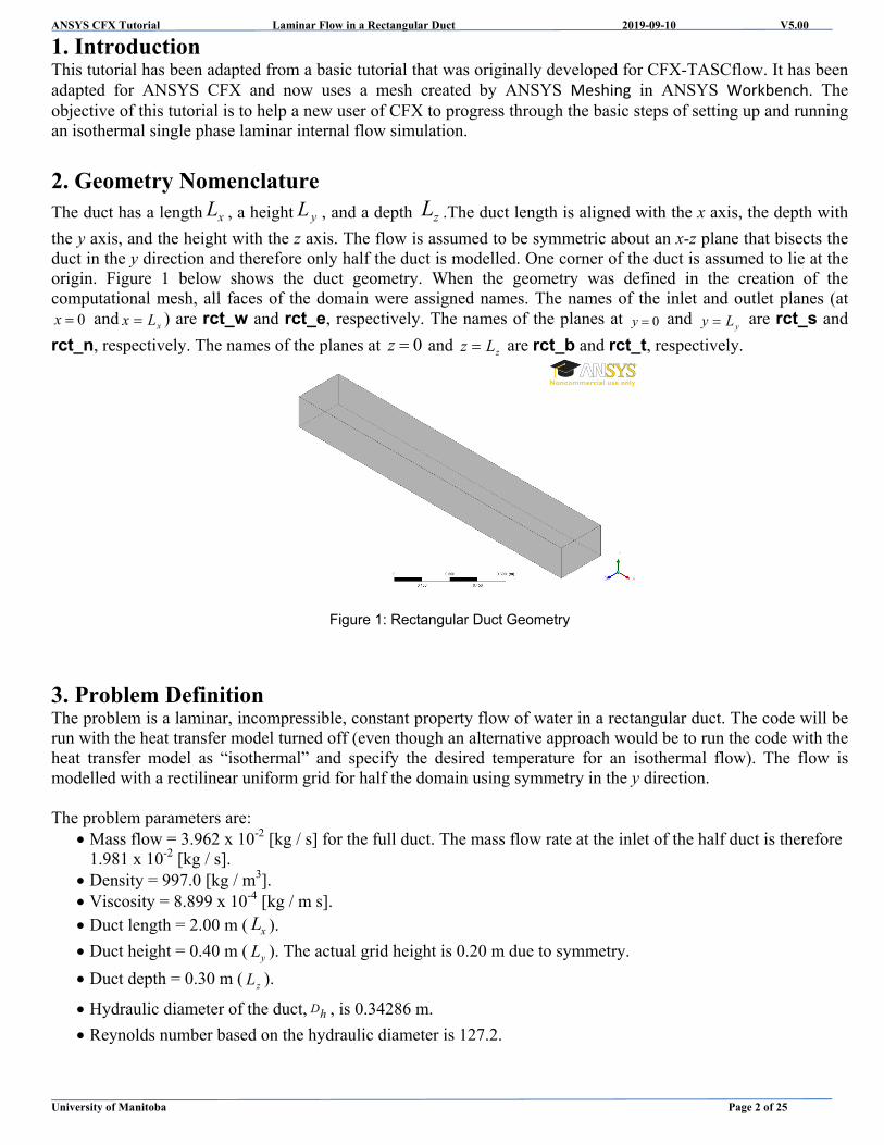
2. Geometry Nomenclature The duct has a length xL , a height yL , and a depth zL .The duct length is aligned with the x axis, the depth with

the y axis, and the height with the z axis. The flow is assumed to be symmetric about an x-z plane that bisects the duct in the y direction and therefore only half the duct is modelled. One corner of the duct is assumed to lie at the origin. Figure 1 below shows the duct geometry. When the geometry was defined in the creation of the computational mesh, all faces of the domain were assigned names. The names of the inlet and outlet planes (at

0x and xLx ) are rct_w and rct_e, respectively. The names of the planes at 0y and yLy are rct_s and

rct_n, respectively. The names of the planes at 0z and zLz are rct_b and rct_t, respectively.

Figure 1: Rectangular Duct Geometry

3. Problem Definition The problem is a laminar, incompressible, constant property flow of water in a rectangular duct. The code will be run with the heat transfer model turned off (even though an alternative approach would be to run the code with the heat transfer model as “isothermal” and specify the desired temperature for an isothermal flow). The flow is modelled with a rectilinear uniform grid for half the domain using symmetry in the y direction. The problem parameters are:

Mass flow = 3.962 x 10-2 [kg / s] for the full duct. The mass flow rate at the inlet of the half duct is therefore 1.981 x 10-2 [kg / s].

Density = 997.0 [kg / m3]. Viscosity = 8.899 x 10-4 [kg / m s]. Duct length = 2.00 m ( xL ).

Duct height = 0.40 m ( yL ). The actual grid height is 0.20 m due to symmetry.

Duct depth = 0.30 m ( zL ).

Hydraulic diameter of the duct, hD , is 0.34286 m.

Reynolds number based on the hydraulic diameter is 127.2.



4. Features This tutorial demonstrates how to: Import a grid (created using ANSYS Meshing) Specify boundary conditions Solve the flow problem Do some post-processing of the results

5. Setup First, create a new directory called cfx-tutorial. Make sure that the path to this directory does not contain any space characters. Spaces in a directory name or path will cause an error message in CFX (in addition, a hyphen cannot be used in the simulation name). Make this new directory your current directory (i.e., “cd” to that directory). The grid for this tutorial has been pre-generated. It was created in ANSYS Workbench using DesignModeler and Meshing. For the purposes of this tutorial, the completed grid will be imported into CFX. The completed grid is in a file called duct.msh that can be copied to your current directory using: cp -p ~engsjo/pub/mech-4822/cfx-tutorial/duct.msh ./ or it can be downloaded (it is inside a zip file called cfxtutorial_duct_msh.zip) from a link in the following web page: http://home.cc.umanitoba.ca/~engsjo/teaching/Tutorials/index.htm#cfxtutorial

6. Assumptions about Running CFX These instructions assume that:

1. The user is connected to a Linux-based server or workstation using ThinLinc. Examples of suitable Linux machines (with suffix .cc.umanitoba.ca) are mars, venus, jupiter, cc01, cc02, cc03, and cc04. or The user is using CFX on a Windows PC.

2. The version of the software is ANSYS CFX v19.2. The CFX launcher can be started under Windows Programs or on Linux by typing: cfx5 & and then using the buttons for CFX-Pre, CFX-Solver, and CFD-Post.

7. Defining the Simulation in CFX-Pre

1. Creating a New Simulation Select File > New Case Simulation Type default is General (click on General in the window and then click OK)



Also click on OK in the following window:

To name the simulation: Select File > Save Case

In the window, set File name to rct_lam.cfx and click Save.

2. Importing the Mesh

Select File > Import > Mesh Files of type: Select Fluent (*cas *msh)



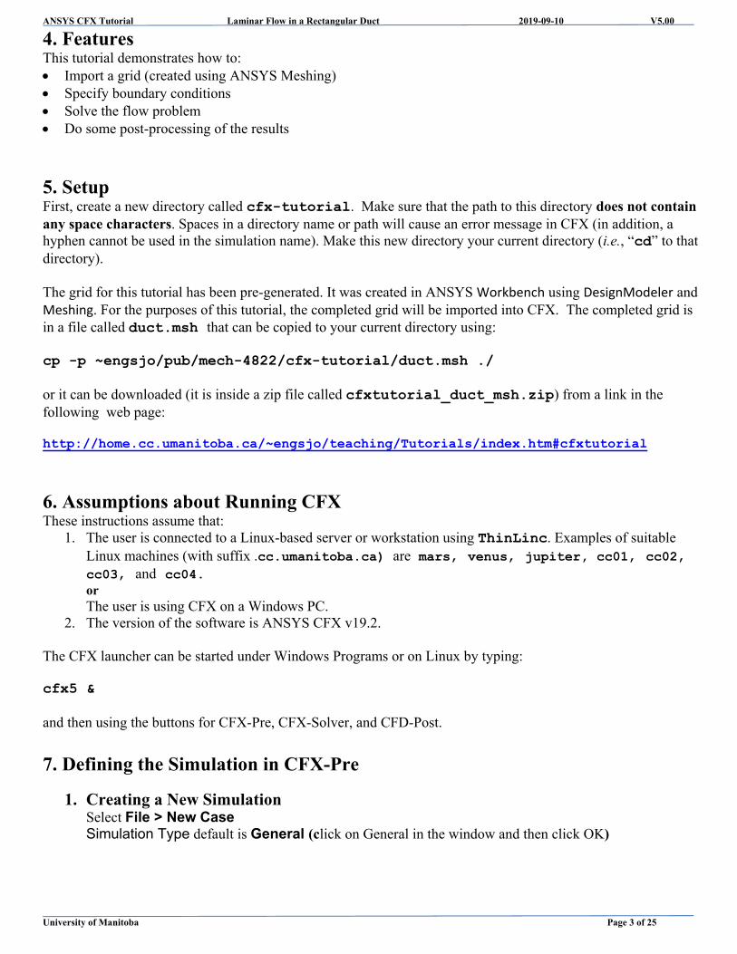
File name: Enter (or browse for) duct.msh Click Open

3. Domain Specification

Select Insert > Domain Name: enter duct Click OK

Under the Domain: duct tab in the Basic Settings tab, click on and then in the Selection Dialog box that appears, click on duct and then Click OK



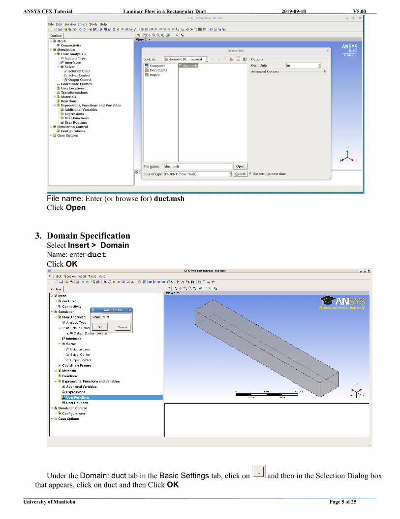
Still under the Basic Settings tab:

Location: this should be DUCT Domain Type: this should be Fluid Domain Coordinate Frame: this should be Coord 0 Fluid and Particle Definitions… this should be Fluid 1 Fluid 1: Option: this should be Material Library

Material: select Water Morphology: Option: this should be Continuous Fluid

Do not click Minimum Volume Fraction. Domain Models Pressure: Reference Pressure: this should be 1 [atm] Buoyancy Model: Option: this should be Non Buoyant Domain Motion: Option: this should be Stationary Mesh Deformation: Option: this should be None



Click Apply

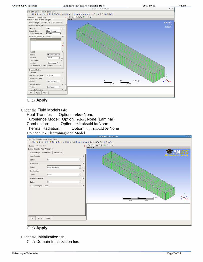
Under the Fluid Models tab:

Heat Transfer: Option: select None Turbulence Model: Option: select None (Laminar) Combustion: Option: this should be None Thermal Radiation: Option: this should be None Do not click Electromagnetic Model.

Click Apply

Under the Initialization tab:

Click Domain Initialization box



Leave all the values as the default values.

Now, Click OK

4. Defining the Inlet Boundary Condition

Select Insert > Boundary Name: enter inlet Click OK

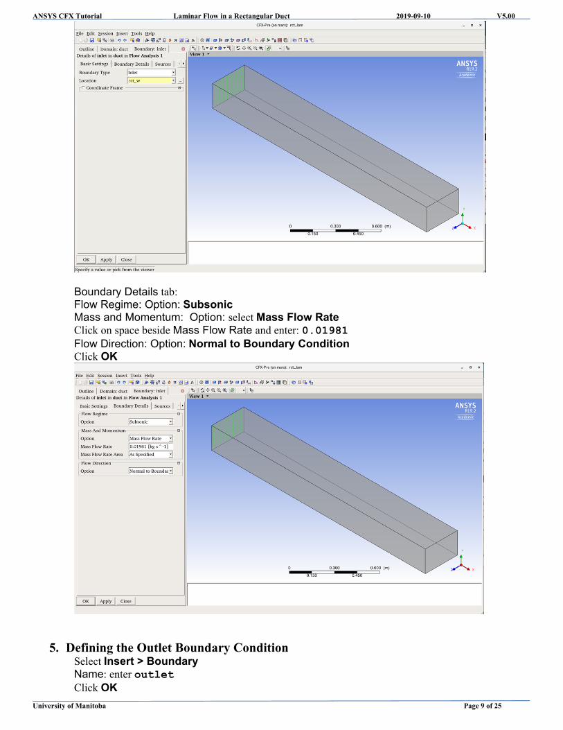
Under Boundary: inlet tab: Basic Settings tab: Boundary Type: select Inlet Location: select rct_w



Boundary Details tab: Flow Regime: Option: Subsonic Mass and Momentum: Option: select Mass Flow Rate Click on space beside Mass Flow Rate and enter: 0.01981 Flow Direction: Option: Normal to Boundary Condition Click OK

5. Defining the Outlet Boundary Condition Select Insert > Boundary Name: enter outlet Click OK



Under Boundary: outlet tab: Basic Settings tab: Boundary Type: select Outlet Location: select rct_e

Boundary Details tab: Flow Regime: Option: Subsonic Mass and Momentum: Option: Average Static Pressure Click on space beside Relative Pressure and enter: 0.0 Leave Pres. Profile Blend at 0.05 Pressure Averaging: Option: Average Over Whole Outlet Click OK



6. Defining the Symmetry Plane Boundary Condition

Select Insert > Boundary Name: enter symmetry Click OK Under Boundary: symmetry tab: Basic Settings tab: Boundary Type: select Symmetry Location: select rct_s Click OK

7. Defining the Walls Boundary Condition Select Insert > Boundary Name: enter walls Click OK Under Boundary: walls tab: Basic Settings tab: Boundary Type: select Wall

Location: click on the icon. In the Selection Dialog window, click on rct_b, then, while holding down the Ctrl key, click on rct_n and rct_t. Click OK.



Boundary Details tab: Mass And Momentum: Option: select No Slip Wall Do not check the box by Wall Velocity Click OK

The overall image of the domain should now appear as:



Note that there is no duct domain “default” in the list. This means that all surfaces have been assigned a boundary condition.

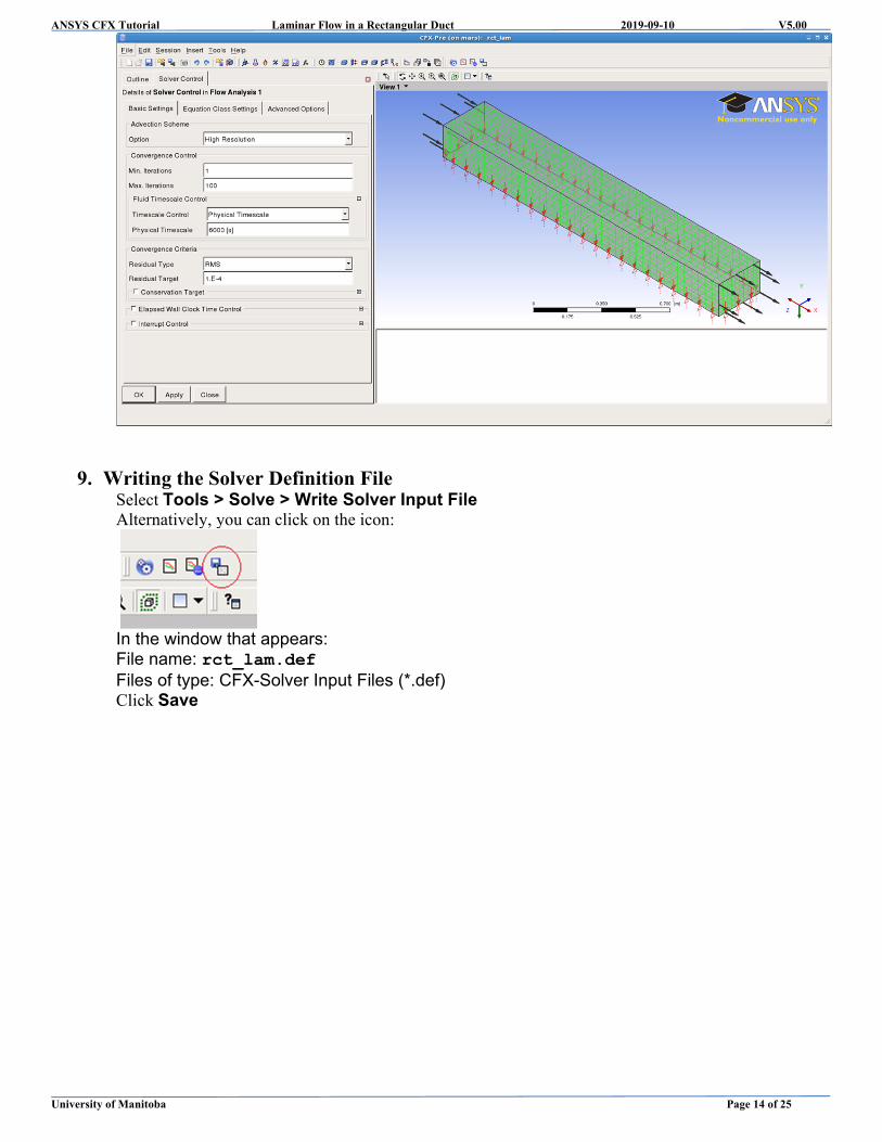
8. Setting the Solver Controls Select Insert > Solver > Solver Control Under Solver Control tab: Details of Solver Control in Flow Analysis 1 tab: Basic Settings tab: Advection Scheme: Option: High Resolution Convergence Control:

Min. Iterations: 1 Max. Iterations: 100

Fluid Timescale Control: Timescale Control: select Physical Timescale Physical Timescale: click in the box and enter 6000

Convergence Criteria: Residual Type: RMS Residual Target: 1.E-4

Leave the boxes unchecked for Conservation Target, Elapsed Wall Clock Time Control, and Interrupt Control. Click OK



9. Writing the Solver Definition File Select Tools > Solve > Write Solver Input File Alternatively, you can click on the icon:

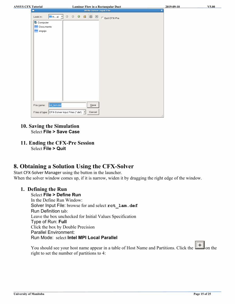
In the window that appears: File name: rct_lam.def Files of type: CFX-Solver Input Files (*.def) Click Save



10. Saving the Simulation Select File > Save Case

11. Ending the CFX-Pre Session

Select File > Quit

8. Obtaining a Solution Using the CFX-Solver Start CFX‐Solver Manager using the button in the launcher. When the solver window comes up, if it is narrow, widen it by dragging the right edge of the window.

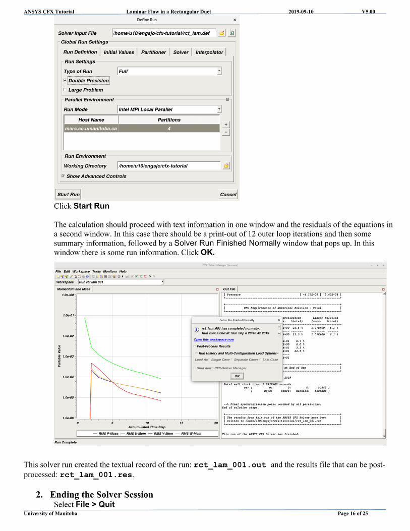
1. Defining the Run Select File > Define Run In the Define Run Window: Solver Input File: browse for and select rct_lam.def Run Definition tab: Leave the box unchecked for Initial Values Specification Type of Run: Full Click the box by Double Precision Parallel Environment: Run Mode: select Intel MPI Local Parallel

You should see your host name appear in a table of Host Name and Partitions. Click the on the right to set the number of partitions to 4:



Click Start Run The calculation should proceed with text information in one window and the residuals of the equations in a second window. In this case there should be a print-out of 12 outer loop iterations and then some summary information, followed by a Solver Run Finished Normally window that pops up. In this window there is some run information. Click OK.

This solver run created the textual record of the run: rct_lam_001.out and the results file that can be post-processed: rct_lam_001.res.

2. Ending the Solver Session Select File > Quit



Viewing the Results using CFD-Post As simple examples of post-processing, this tutorial illustrates how to create a graph of a velocity profile at the duct exit and a velocity vector plot on the plane of symmetry. There are many other features available in CFD-Post. For more details on these features, consult the course instructor and teaching assistant, as well as the on-line CFD-Post help. To begin using CFD-Post type: Cfx5post –gr mesa&

1. Loading the Results File Select File > Load Results In the file browser window, click on rct_lam_001.res and then click Open.

2. Creating a Line at the Exit Plane Select Insert > Location > Line Name: enter Exit Line Click OK



A sidebar entitled “Details of Exit Line” should appear. Geometry tab: Domains: All Domains Definition: Method: Two Points Point 1: enter 2, 0, 0 Point 2: enter 2, 0, 0.3 Line Type: click on circle for Cut Click on Apply

(Aside: In the future, we will use Line Type Sample and specify a number of points to sample.) A yellow line will appear at the end of the duct image in the 3D viewer. After zooming, it should appear like:



In order to zoom in, you can use some of the icons at the top of the 3D viewer window:

To zoom click the (zoom) or (zoom box) icons. You can also use the pan icon: to move the image around and a scroll wheel on a mouse to zoom. You can also change the view by right clicking on the 3D viewer window and choosing a Predefined Camera. If you want to see the entire duct

again, click on the fit view icon: .

3. Creating a Graph (Chart) of a Velocity Profile at the Exit Select Insert > Chart Name: U Velocity versus z Click OK Under Details of U Velocity versus z: General tab: Type: XY Title: U Velocity at the Exit Caption: Exit Velocity Graph Data Series tab: For Series 1: Name: click in the box and enter Exit Line Profile Location: select Exit Line X Axis tab:



Variable: select Z Leave the box checked for Determine ranges automatically Y Axis tab: Variable: select Velocity u Click on the circle for Hybrid Leave the box checked for Determine ranges automatically Click on Apply

You should see the chart shown below in the right window (Chart Viewer).

The data used in this chart can also be exported to a spreadsheet program by using the export feature. To do this:

Click Export File name: enter u_exit_profile.csv File Type: Comma Separated Values (*.csv) Click on Save



The file created, when loaded into Excel (and formatted with more decimals for column A and scientific notation for column B), looks like:

These data can also be exported in a text file format for plotting with gnuplot or other plotting software.

4. Creating a Velocity Vector Plot

Click on the 3D Viewer tab. Select Insert > Vector Name: enter Symm Plane Vectors Click OK A sidebar entitled “Details of Symm Plane Vectors” should appear.



Geometry tab: Domains: All Domains Definition: Locations: select symmetry Sampling: Vertex Reduction: Reduction Factor Factor: select 1.0 Variable: Velocity Boundary Data: Click on the circle for Hybrid Projection: None Click on Apply

The vector plot below should appear in the 3D Viewer window. The domain was zoomed in for the image.



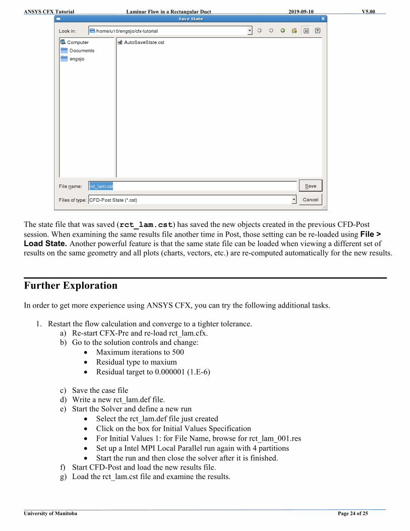
3. Ending the CFD-Post Session Select File > Quit Click on Save & Quit

File name: enter rct_lam.cst Files of type: CFD-Post State (*.cst) Click on Save



The state file that was saved (rct_lam.cst) has saved the new objects created in the previous CFD-Post session. When examining the same results file another time in Post, those setting can be re-loaded using File > Load State. Another powerful feature is that the same state file can be loaded when viewing a different set of results on the same geometry and all plots (charts, vectors, etc.) are re-computed automatically for the new results.

Further Exploration In order to get more experience using ANSYS CFX, you can try the following additional tasks.

1. Restart the flow calculation and converge to a tighter tolerance. a) Re-start CFX-Pre and re-load rct_lam.cfx. b) Go to the solution controls and change:

Maximum iterations to 500 Residual type to maxium Residual target to 0.000001 (1.E-6)

c) Save the case file d) Write a new rct_lam.def file. e) Start the Solver and define a new run

Select the rct_lam.def file just created Click on the box for Initial Values Specification For Initial Values 1: for File Name, browse for rct_lam_001.res Set up a Intel MPI Local Parallel run again with 4 partitions Start the run and then close the solver after it is finished.

f) Start CFD-Post and load the new results file. g) Load the rct_lam.cst file and examine the results.



2. Add energy equation calculation and thermal boundary conditions.

a) Re-start CFX-Pre and re-load rct_lam.cfx. b) In the Outline below Analysis Type, double click on “duct”. Under “Domain: duct”, click on the

Fluid Models tab. Change the “Heat Transfer” Option to “Thermal Energy”. Click OK. You will see an error message appear that refers to boundary conditions. This means you need to add thermal boundary conditions. You will add an inlet temperature and a wall temperature. The symmetry and outlet conditions do not need to be changed.

c) Double click on “inlet” below duct under Analysis Type. Click on the Boundary Details tab. Under Heat Transfer Option, select Static Temperature.

Then, click in the box beside Static Temperature and enter 300 (the units should be K). Click OK.

d) Double click on “walls” below duct under Analysis Type. Click on the Boundary Details tab. Under Heat Transfer Option, select Heat Flux. Then,

click in the box beside Heat Flux in and enter 2000 (the units should be W/m2). Click OK. e) Use File > Save Case As to save the current setup as rct_lam_thermal.cfx. f) Write a Solver Input File: rct_lam_thermal.def. g) Start the Solver and define a new run

Select the rct_lam_thermal.def file just created Do not use Initial Values Specification Use double precision Set up a Intel MPI Local Parallel run again with 4 partitions Start the run and then close the solver after it is finished.

h) Start CFD-Post and load the new results file. i) Load the rct_lam.cst file and examine the results. j) Try creating a contour plot of Temperature at the outlet face. k) Save the modified state as rct_lam_thermal.cst. l) Examine the temperature results. Create a new chart that is the temperature profile at the Exit Line

created earlier. m) Create a new line that goes down the centre of the duct. Create a chart that plots the temperature

along this line.

ansys cfx tutorial laminar flow in a rectangular...

Documents