ansys tutorialsintroduction.docx

7/27/2019 ANSYS TUTORIALSIntroduction.docx

http://slidepdf.com/reader/full/ansys-tutorialsintroductiondocx 1/53

Introduction: In this example you will learn to model a composite material and analyze one

dimensional conduction properties. Using ANSYS will allow you to output thetemperature distribution in an extremely simple and accurate way.

Problem Description:

We are modeling heat transfer in a block with a gap filled with different gases. All units are S.I. Boundary Conditions:

1) The left side of the block has a constant temperature of 400 K.2) The right side of the block has convection (h=20 W/m-K ; T= 300

K) 3) The Al section generates heat at a rate of 200 W/m3 4) The He section absorbs heat at a rate of 175 W/m3

Material Properties: Aluminum(1st layer): K Al = 235 W/m*K

Helium(2nd layer): K He = 0.1513 W/m*K Copper(3rd layer): K Cu = 400 W/m*K

Dimensions Length = 3 m Width = 3 m Thickness of each Layer = 1 m

Objective: Find the nodal temperature distribution and the rate of heat loss fromthe furnace.

Figure:

Basic Outline of the Problem:

Preprocessing: 1. Start ANSYS. 2. Create areas through keypoints. 3. Define the material properties. 4. Define element type. (Quad 8node 77 element, which is a 2-D element for heattransfer analysis.) 5. Specify meshing controls / Mesh the areas to create nodes and elements.

Solution:



6. Specify boundary conditions.

7. Solve.

Postprocessing: 8. List the results of the temperature distribution. 9. Plot the results of the temperature distribution.

Exit: 10. Exit the ANSYS program, saving all data.

Starting ANSYS:

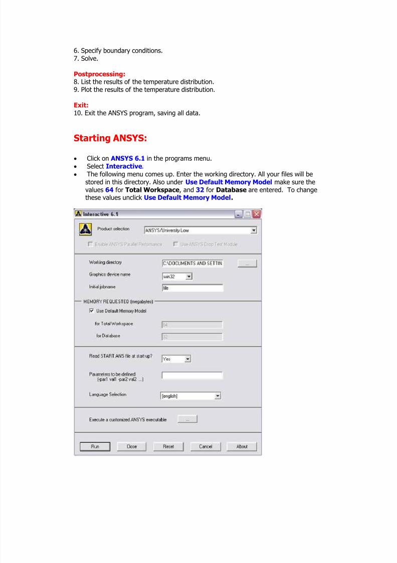
Click on ANSYS 6.1 in the programs menu. Select Interactive. The following menu comes up. Enter the working directory. All your files will be

stored in this directory. Also under Use Default Memory Model make sure thevalues 64 for Total Workspace, and 32 for Database are entered. To change

these values unclick Use Default Memory Model.



Click RUN

Modeling the Structure:

Go to the ANSYS Utility Menu (the top bar). Click Workplane>WP Settings… The following widow comes up: (notice the numbers are different)

Check the Cartesian and Grid Only buttons Enter the values shown in the figure above. Click OK

Go to the ANSYS Utility Menu (the top bar). Click Workplane>Display WorkingPlane. This will display the working grid on the workspace.

Use Utility Menu>PlotCtrls>Pan Zoom Rotate to display the grid as shown in

the next step below.

Next, go to the ANSYS Main Menu (on the left hand side of the screen) and click Preprocessor>Modeling>Create>Keypoints>On Working Plane.

The following window comes up:



Click on the working plane below to select the points (they follow the dimensionsexplained in the beginning, (1m x 3m). After setting the workplane settings in thebeginning, you should be aware that each line on the plane equals to 1m. When

done, click OK.



Now you have created the points to make the block.

Now select Preprocessor>Modeling>Create>Areas>Arbitrary>ThroughKPs. A window will now appear on the left of the screen.

Select the points that form the 1st section. Click Apply such that it is formedseparate from the other two areas.

Repeat the step of selecting the KPs that make up each area, and clicking Applyuntil all three layers are defined. (Click OK for the last one)

The model should look like this now: (note, you have a black background)

Material Properties:

Now that we have built the model, material properties need to be defined suchthat ANSYS understands how heat travels through this composite solid.

Go to the ANSYS Main Menu Select Preferences. We will set up the drop menus only to include thermal tasks, to

make everything easy to navigate.



Select Thermal and hit ok. Now you are ready. Click Preprocessor>Material Props>Material Models.

The pop-up window will now look like this:

In the window that comes up, select Material>New Material



Hit OK. Repeat the process for the third material. (repeat the last step once more) Choose Thermal>Conductivity>Isotropic. The following window comes up:

Fill in 235 for Thermal conductivity. Click OK . This is the Thermal Conductivity of

Al. Now repeat the steps of clicking Thermal>Conductivity>Isotropic and then

defining the Thermal Conductivity as 0.1513 for the Model 2. You have now defined the k value of Helium. Define the last section and this time use K = 400. This is the Thermal

Conductivity of Copper. Now exit the “Define Material Model Behavior” Window.

Element Properties:

Now that we’ve defined what material ANSYS will be analyzing, we have to define

how ANSYS should analyze our block.

Click Preprocessor>Element Type>Add/Edit/Delete... In the 'ElementTypes' window that opens click on Add... The following window opens:



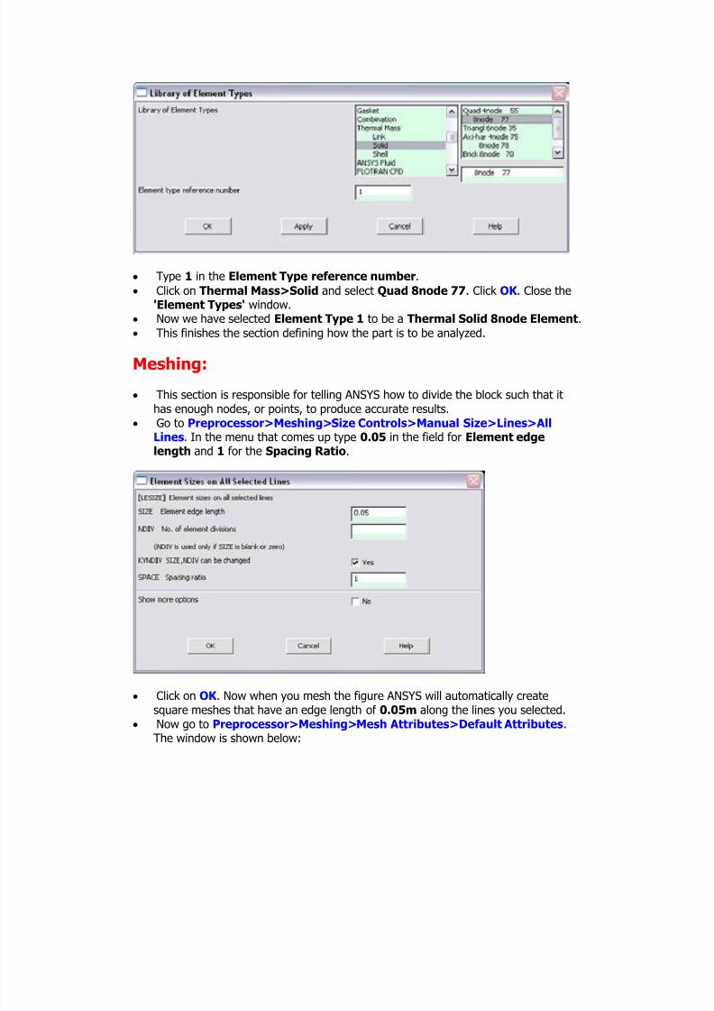
Type 1 in the Element Type reference number. Click on Thermal Mass>Solid and select Quad 8node 77. Click OK . Close the

'Element Types' window.

Now we have selected Element Type 1 to be a Thermal Solid 8node Element.

This finishes the section defining how the part is to be analyzed.

Meshing:

This section is responsible for telling ANSYS how to divide the block such that it

has enough nodes, or points, to produce accurate results. Go to Preprocessor>Meshing>Size Controls>Manual Size>Lines>All

Lines. In the menu that comes up type 0.05 in the field for Element edgelength and 1 for the Spacing Ratio.

Click on OK . Now when you mesh the figure ANSYS will automatically create

square meshes that have an edge length of 0.05m along the lines you selected. Now go to Preprocessor>Meshing>Mesh Attributes>Default Attributes.

The window is shown below:



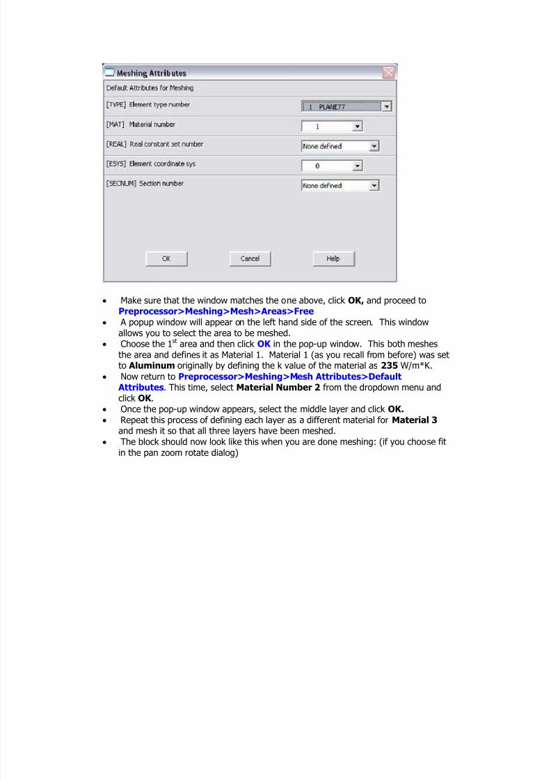
Make sure that the window matches the one above, click OK, and proceed toPreprocessor>Meshing>Mesh>Areas>Free

A popup window will appear on the left hand side of the screen. This window

allows you to select the area to be meshed. Choose the 1st area and then click OK in the pop-up window. This both meshes

the area and defines it as Material 1. Material 1 (as you recall from before) was setto Aluminum originally by defining the k value of the material as 235 W/m*K.

Now return to Preprocessor>Meshing>Mesh Attributes>Default Attributes. This time, select Material Number 2 from the dropdown menu andclick OK .

Once the pop-up window appears, select the middle layer and click OK. Repeat this process of defining each layer as a different material for Material 3

and mesh it so that all three layers have been meshed. The block should now look like this when you are done meshing: (if you choose fit

in the pan zoom rotate dialog)



Boundary Conditions and Constraints:

Now that we have modeled the block and defined how ANSYS is to analyze theblock we will apply the appropriate Boundary Conditions. ANSYS refers to allBoundary Conditions under the Loads category, so remember that when looking forcommands within the main menu…

Go to Preprocessor>Loads>Define Loads>Apply>Thermal (from here onecan apply any of the loads, or Boundary Conditions, offered by ANSYS.)

Apply Constant Temperature

Now we’ll apply the given temperature boundary condition on the right side of theblock.

This time, within the Thermal Load category select Temperature>On Lines. A popup window will appear on the left hand side of the screen. This window

allows you to select the line you wish the load to be applied to. Click the innermost boundary of the block and then OK . Enter 400 in the popup window as the set temperature for the left edge of the

first section:

Apply Convection



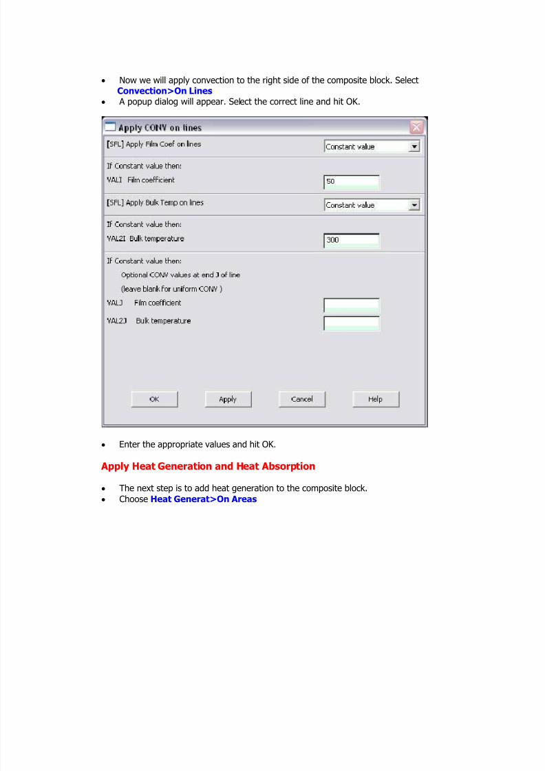
Now we will apply convection to the right side of the composite block. SelectConvection>On Lines

A popup dialog will appear. Select the correct line and hit OK.

Enter the appropriate values and hit OK.

Apply Heat Generation and Heat Absorption

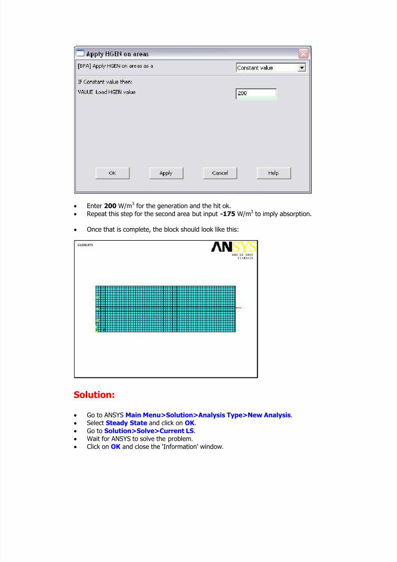
The next step is to add heat generation to the composite block. Choose Heat Generat>On Areas



Enter 200 W/m3 for the generation and the hit ok. Repeat this step for the second area but input -175 W/m3 to imply absorption.

Once that is complete, the block should look like this:

Solution:

Go to ANSYS Main Menu>Solution>Analysis Type>New Analysis. Select Steady State and click on OK .

Go to Solution>Solve>Current LS.

Wait for ANSYS to solve the problem.

Click on OK and close the 'Information' window.



Post-Processing:

This section is designed so that one can present the results of their analysis in themost appropriate way. This presentation can be in the form of tabulated nodalvalues, curves, etc.

Go to the ANSYS Main Menu. Click General Postprocessing>List

Results>Nodal Solution. The following window will come up:

Select DOF solution and Temperature. Click on OK . The nodal temperatures

will be listed as follows:

Within this window one can numerically find the maximum and minimum value of the temperature within the block. Note that you may have nodes in different

places. Therefore your first displayed temperatures might not be the same as theones shown above. If you scroll down you should find everything.

Modification / Plotting the Results:

The last section displayed the numerical results, but some people prefer a plotpresentation of the temperatures on the block over the numerical results. This ishow you go about doing that…



First go to General Postprocessing>Plot Results>Contour Plot>Nodal

Solution. The following window will come up:

Select DOF solution and Temperature to be plotted and click OK . The outputwill be like this:

This is the Final Solution To find extra information on Saving an ANSYS model see the Appendix on the

ANSYS tutorial mainpage.

Saving Projects

Simply go to Utility Menu>File>Save As… and save the project using the

desired filename. To open the file later, run Interactive (the first thing explained in



this tutorial) as usual, and when that is done, go to Utility Menu>File>ResumeFrom… and choose the saved job from the directory it is saved in.

Solid Model Creation

Introduction This tutorial is the last of three basic tutorials devised to illustrate commom features in ANSYS.Each tutorial builds upon techniques covered in previous tutorials, it is therefore essential that

you complete the tutorials in order.

The Solid Modelling Tutorial will introduce various techniques which can be used in ANSYS to

create solid models. Filleting, extrusion/sweeping, copying, and working plane orientation will

be covered in detail.

Two Solid Models will be created within this tutorial.

Problem Description A

We will be creating a solid model of the pulley shown in the following figure.



Geometry Generation

We will create this model by first tracing out the cross section of the pulley and then sweeping

this area about the y axis.

Creation of Cross Sectional Area

1. Create 3 Rectangles

Main Menu > Preprocessor > (-Modeling-) Create > Rectangle > By 2

Corners BLC4, XCORNER, YCORNER, WIDTH, HEIGHT

The geometry of the rectangles:

Rectangle 1 Rectangle 2 Rectangle 3

WP X (XCORNER) 2 3 8

WP Y (YCORNER) 0 2 0



WIDTH 1 5 0.5

HEIGHT 5.5 1 5

You should obtain the following:

2. Add the Areas

Main Menu > Preprocessor > (-Modeling-) Operate > (-Boolean-) Add >

Areas AADD, ALL

ANSYS will label the united area as AREA 4 and the previous three areas will be

deleted.

3. Create the rounded edges using circles

Preprocessor > (-Modeling-) Create > (-Areas-) Circle > Solid circles CYL4,XCENTER,YCENTER,RAD

The geometry of the circles:

Circle 1 Circle 2

WP X (XCENTER) 3 8.5

WP Y (YCENTER) 5.5 0.2

RADIUS 0.5 0.2

4. Subtract the large circle from the base



Preprocessor > Operate > Subtract > Areas ASBA,BASE,SUBTRACT

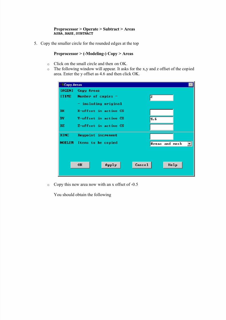
5. Copy the smaller circle for the rounded edges at the top

Preprocessor > (-Modeling-) Copy > Areas

o Click on the small circle and then on OK.o The following window will appear. It asks for the x,y and z offset of the copied

area. Enter the y offset as 4.6 and then click OK.

o Copy this new area now with an x offset of -0.5

You should obtain the following



6. Add the smaller circles to the large area.

Preprocessor > Operate > Add > Areas AADD,ALL

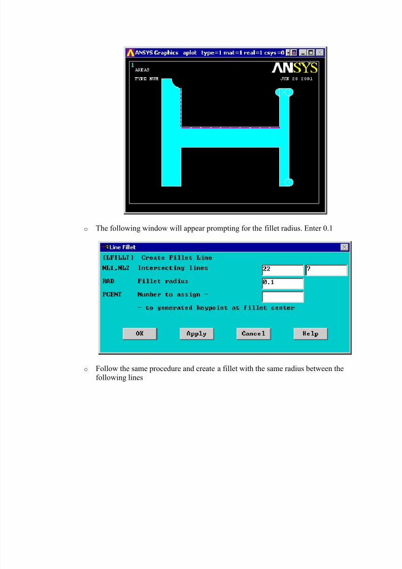
7. Fillet the inside edges of the top half of the area

Preprocessor > Create > (-Lines-) Line Fillet

o Select the two lines shown below and click on OK.



o The following window will appear prompting for the fillet radius. Enter 0.1

o Follow the same procedure and create a fillet with the same radius between thefollowing lines



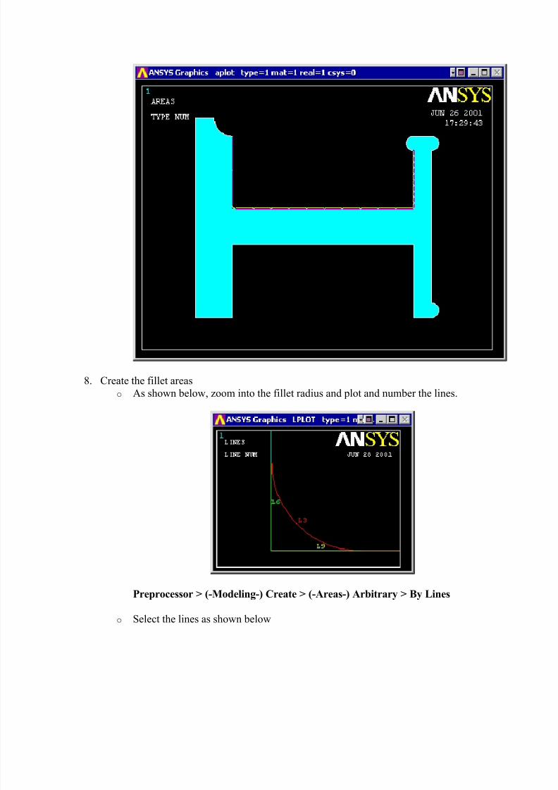
8. Create the fillet areaso As shown below, zoom into the fillet radius and plot and number the lines.

Preprocessor > (-Modeling-) Create > (-Areas-) Arbitrary > By Lines

o Select the lines as shown below



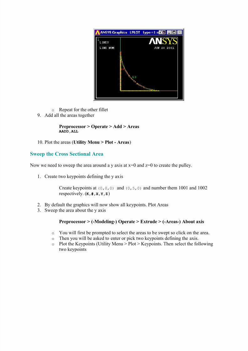
o Repeat for the other fillet

9. Add all the areas together

Preprocessor > Operate > Add > Areas AADD,ALL

10. Plot the areas (Utility Menu > Plot - Areas)

Sweep the Cross Sectional Area

Now we need to sweep the area around a y axis at x=0 and z=0 to create the pulley.

1. Create two keypoints defining the y axis

Create keypoints at (0,0,0) and (0,5,0) and number them 1001 and 1002

respectively. (K,#,X,Y,Z)

2. By default the graphics will now show all keypoints. Plot Areas3. Sweep the area about the y axis

Preprocessor > (-Modeling-) Operate > Extrude > (-Areas-) About axis

o You will first be prompted to select the areas to be swept so click on the area.o Then you will be asked to enter or pick two keypoints defining the axis.

o

Plot the Keypoints (Utility Menu > Plot > Keypoints. Then select the followingtwo keypoints



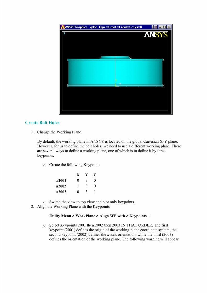
o The following window will appear prompting for sweeping angles. Click on OK.

You should now see the following in the graphics screen.



Create Bolt Holes

1. Change the Working Plane

By default, the working plane in ANSYS is located on the global Cartesian X-Y plane.

However, for us to define the bolt holes, we need to use a different working plane. There

are several ways to define a working plane, one of which is to define it by three

keypoints.

o Create the following Keypoints

X Y Z

#2001 0 3 0

#2002 1 3 0

#2003 0 3 1

o Switch the view to top view and plot only keypoints.

2. Align the Working Plane with the Keypoints

Utility Menu > WorkPlane > Align WP with > Keypoints +

o Select Keypoints 2001 then 2002 then 2003 IN THAT ORDER. The first

keypoint (2001) defines the origin of the working plane coordinate system, the

second keypoint (2002) defines the x-axis orientation, while the third (2003)defines the orientation of the working plane. The following warning will appear



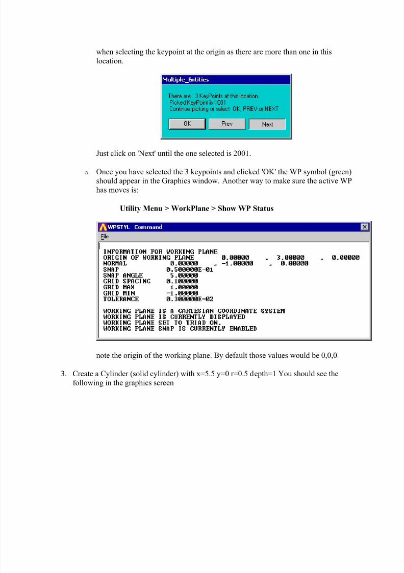
when selecting the keypoint at the origin as there are more than one in this

location.

Just click on 'Next' until the one selected is 2001.

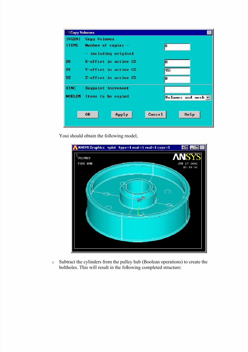
o Once you have selected the 3 keypoints and clicked 'OK' the WP symbol (green)should appear in the Graphics window. Another way to make sure the active WP

has moves is:

Utility Menu > WorkPlane > Show WP Status

note the origin of the working plane. By default those values would be 0,0,0.

3. Create a Cylinder (solid cylinder) with x=5.5 y=0 r=0.5 depth=1 You should see the

following in the graphics screen



We will now copy this volume so that we repeat it every 45 degrees. Note that you must

copy the cylinder before you use boolean operations to subtract it because you cannotcopy an empty space.

4. We need to change active CS to cylindrical Y

Utility Menu > WorkPlane > Change Active CS to > Global Cylindrical Y This will allow us to copy radially about the Y axis

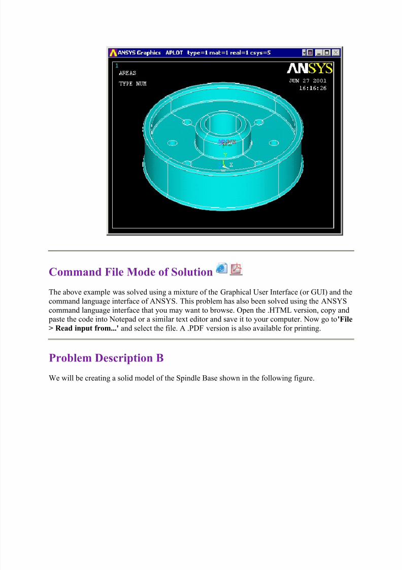
5. Create 8 bolt Holes

Preprocessor > Copy > Volumes

o Select the cylinder volume and click on OK. The following window will appear;

fill in the blanks as shown,



Youi should obtain the following model,

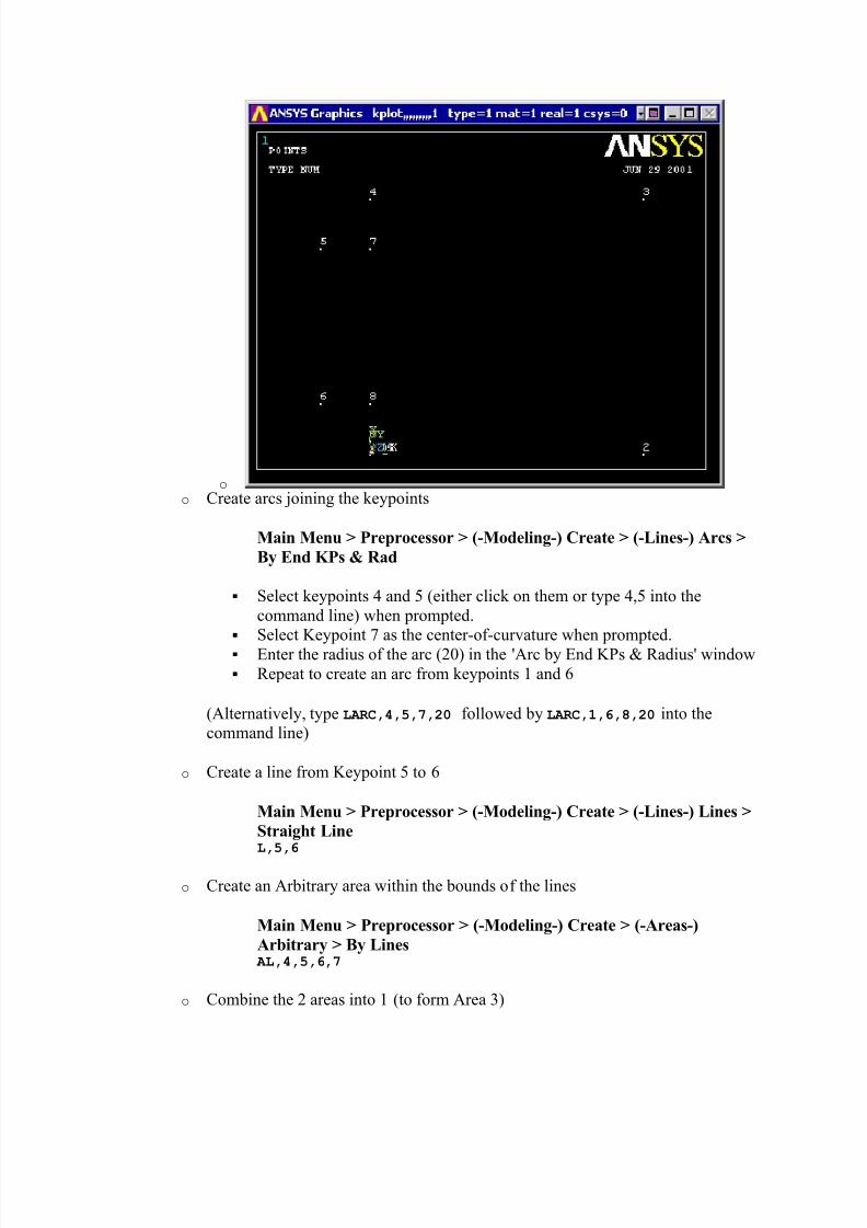
o Subtract the cylinders from the pulley hub (Boolean operations) to create the

boltholes. This will result in the following completed structure:



Command File Mode of Solution

The above example was solved using a mixture of the Graphical User Interface (or GUI) and the

command language interface of ANSYS. This problem has also been solved using the ANSYScommand language interface that you may want to browse. Open the .HTML version, copy and paste the code into Notepad or a similar text editor and save it to your computer. Now go to 'File

> Read input from...' and select the file. A .PDF version is also available for printing.

Problem Description B

We will be creating a solid model of the Spindle Base shown in the following figure.

http://www.mece.ualberta.ca/tutorials/ansys/CL/CBT/Solid/Print.pdf

http://www.mece.ualberta.ca/tutorials/ansys/CL/CBT/Solid/Print.html







Geometry Generation

We will create this model by creating the base and the back and then the rib.

Create the Base

1. Create the base rectangle

WP X (XCORNER) WP Y (YCORNER) WIDTH HEIGHT

0 0 109 102

2. Create the curved edge (using keypoints and lines to create an area)o Create the following keypoints

X Y Z

Keypoint 5 -20 82 0

Keypoint 6 -20 20 0

Keypoint 7 0 82 0

Keypoint 8 0 20 0

o You should obtain the following:



o o Create arcs joining the keypoints

Main Menu > Preprocessor > (-Modeling-) Create > (-Lines-) Arcs >

By End KPs & Rad

Select keypoints 4 and 5 (either click on them or type 4,5 into the

command line) when prompted.

Select Keypoint 7 as the center-of-curvature when prompted.

Enter the radius of the arc (20) in the 'Arc by End KPs & Radius' window

Repeat to create an arc from keypoints 1 and 6

(Alternatively, type LARC,4,5,7,20 followed by LARC,1,6,8,20 into thecommand line)

o Create a line from Keypoint 5 to 6

Main Menu > Preprocessor > (-Modeling-) Create > (-Lines-) Lines >

Straight Line L,5,6

o Create an Arbitrary area within the bounds of the lines

Main Menu > Preprocessor > (-Modeling-) Create > (-Areas-)

Arbitrary > By Lines AL,4,5,6,7

o Combine the 2 areas into 1 (to form Area 3)



Main Menu > Preprocessor > (-Modeling-) Operate > (-Booleans-)

Add > Volumes AADD,1,2

3. You should obtain the following image:

4. 5. Create the 4 holes in the base

We will make use of the 'copy' feature in ANSYS to create all 4 holes

o Create the bottom left circle (XCENTER=0, YCENTER=20, RADIUS=10)o Copy the area to create the bottom right circle (DX=69)

(AGEN,# Copies (include original),Area#,Area2# (if 2 areas to be

copied),DX,DY,DZ)

o Copy both circles to create the upper circles (DY=62)o Subtract the three circles from the main base

( ASBA,3,ALL)




6. Extrude the base

Preprocessor > (-Modeling-) Operate > Extrude > (-Areas-) Along Normal

The following window will appear once you select the area

o Fill in the window as shown (length of extrusion = 26mm). Note, to extrude the

area in the negative z direction you would simply enter -26.

(Alternatively, type VOFFST,6,26 into the command line)

Create the Back

1. Change the working plane



As in the previous example, we need to change the working plane. You may have

observed that geometry can only be created in the X-Y plane. Therefore, in order to

create the back of the Spindle Base, we need to create a new working plane where the X-Y plane is parallel to the back. Again, we will define the working plane by aligning it to 3

Keypoints.

o Create the following keypoints

X Y Z

#100 109 102 0

#101 109 2 0

#102 159 102 sqrt(3)/0.02

o Align the working plane to the 3 keypoints

Recall when defining the working plane; the first keypoint defines the origin, thesecond keypoint defines the x-axis orientation, while the third defines the

orientation of the working plane.

(Alternatively, type KWPLAN,1,100,101,102 into the command line)

2. Create the back area

o Create the base rectangle (XCORNER=0, YCORNER=0, WIDTH=102,

HEIGHT=180)o Create a circle to obtain the curved top (XCENTER=51, YCENTER=180,

RADIUS=51)o Add the 2 areas together

3.

Extrude the area (length of extrusion = 26mm)

Preprocessor > (-Modeling-) Operate > Extrude > (-Areas-) Along Normal VOFFST,27,26

4. Add the base and the back together o Add the two volumes together

Preprocessor > (-Modeling-) Operate > (-Booleans-) Add > Volumes VADD,1,2

You should now have the following geometry



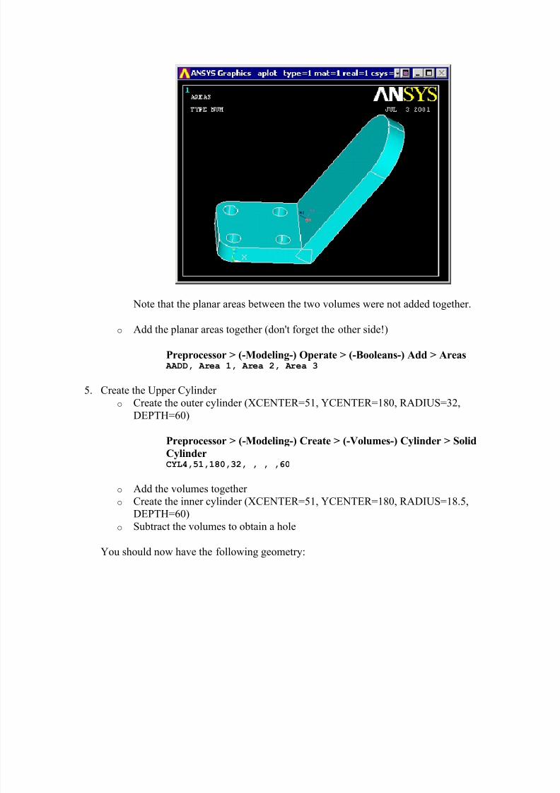
Note that the planar areas between the two volumes were not added together.

o Add the planar areas together (don't forget the other side!)

Preprocessor > (-Modeling-) Operate > (-Booleans-) Add > Areas AADD, Area 1, Area 2, Area 3

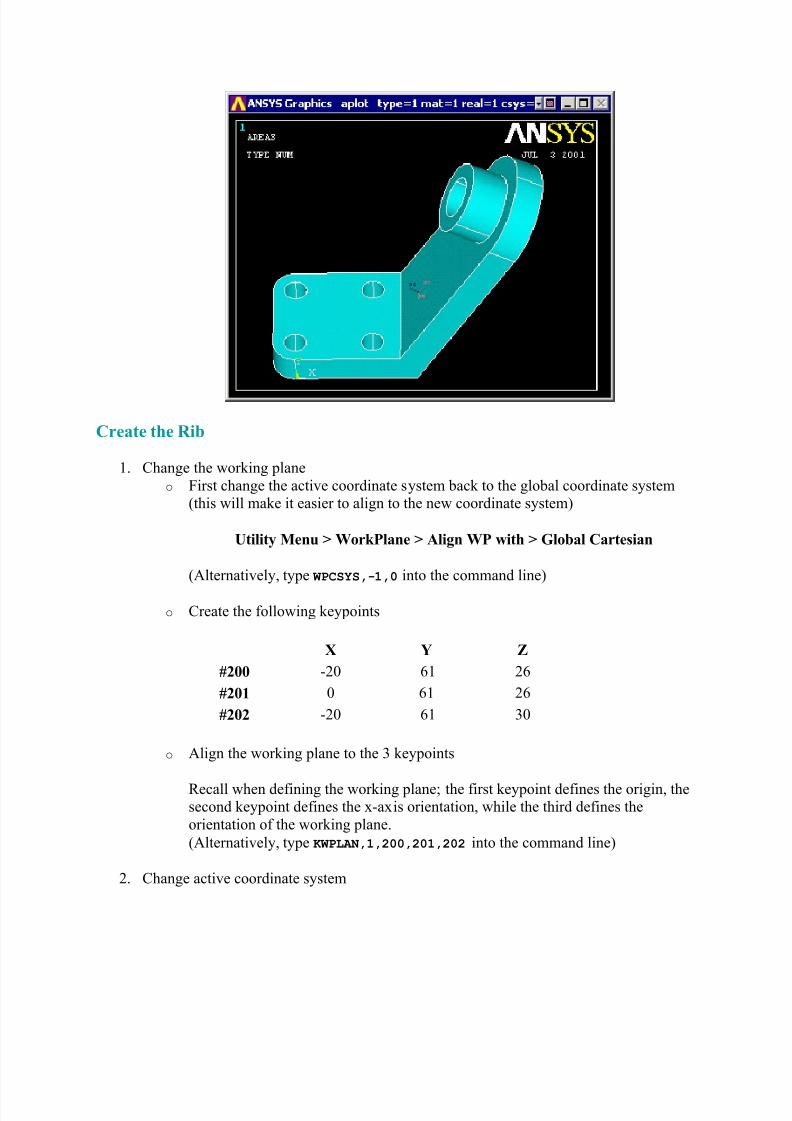
5. Create the Upper Cylinder

o Create the outer cylinder (XCENTER=51, YCENTER=180, RADIUS=32,

DEPTH=60)

Preprocessor > (-Modeling-) Create > (-Volumes-) Cylinder > Solid

CylinderCYL4,51,180,32, , , ,60

o Add the volumes together o Create the inner cylinder (XCENTER=51, YCENTER=180, RADIUS=18.5,

DEPTH=60)

o Subtract the volumes to obtain a hole

You should now have the following geometry:



Create the Rib

1. Change the working planeo First change the active coordinate system back to the global coordinate system

(this will make it easier to align to the new coordinate system)

Utility Menu > WorkPlane > Align WP with > Global Cartesian

(Alternatively, type WPCSYS,-1,0 into the command line)

o Create the following keypoints

X Y Z

#200 -20 61 26

#201 0 61 26

#202 -20 61 30

o Align the working plane to the 3 keypoints

Recall when defining the working plane; the first keypoint defines the origin, thesecond keypoint defines the x-axis orientation, while the third defines the

orientation of the working plane.

(Alternatively, type KWPLAN,1,200,201,202 into the command line)

2. Change active coordinate system



We now need to update the coordiante system to follow the working plane changes (ie

make the new Work Plane origin the active coordinate)

Utility Menu > WorkPlane > Change Active CS to > Working PlaneCSYS,4

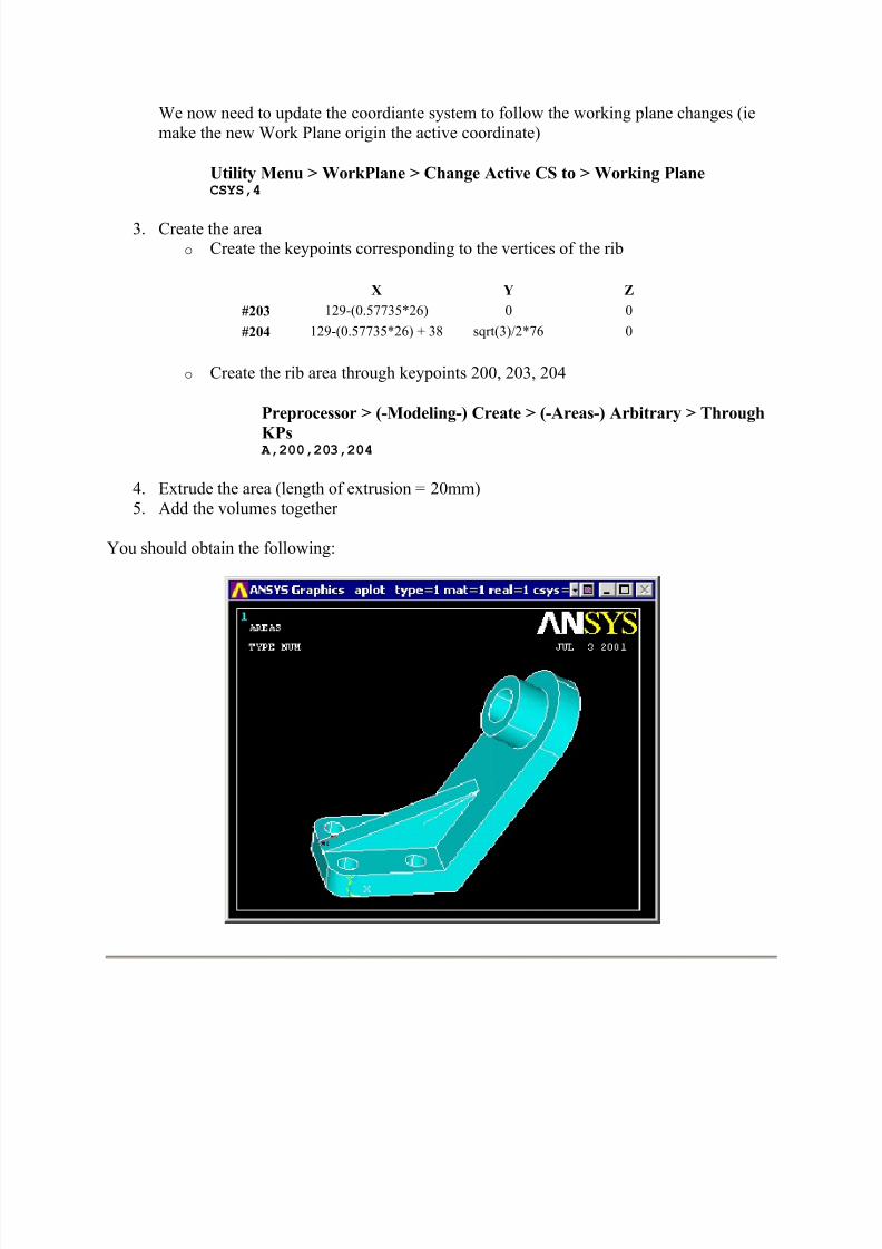
3. Create the areao Create the keypoints corresponding to the vertices of the rib

X Y Z

#203 129-(0.57735*26) 0 0

#204 129-(0.57735*26) + 38 sqrt(3)/2*76 0

o Create the rib area through keypoints 200, 203, 204

Preprocessor > (-Modeling-) Create > (-Areas-) Arbitrary > Through

KPs A,200,203,204

4. Extrude the area (length of extrusion = 20mm)

5. Add the volumes together




Modelling Using Axisymmetry

Introduction

This tutorial was completed using ANSYS 7.0 This tutorial is intended to outline the stepsrequired to create an axisymmetric model.

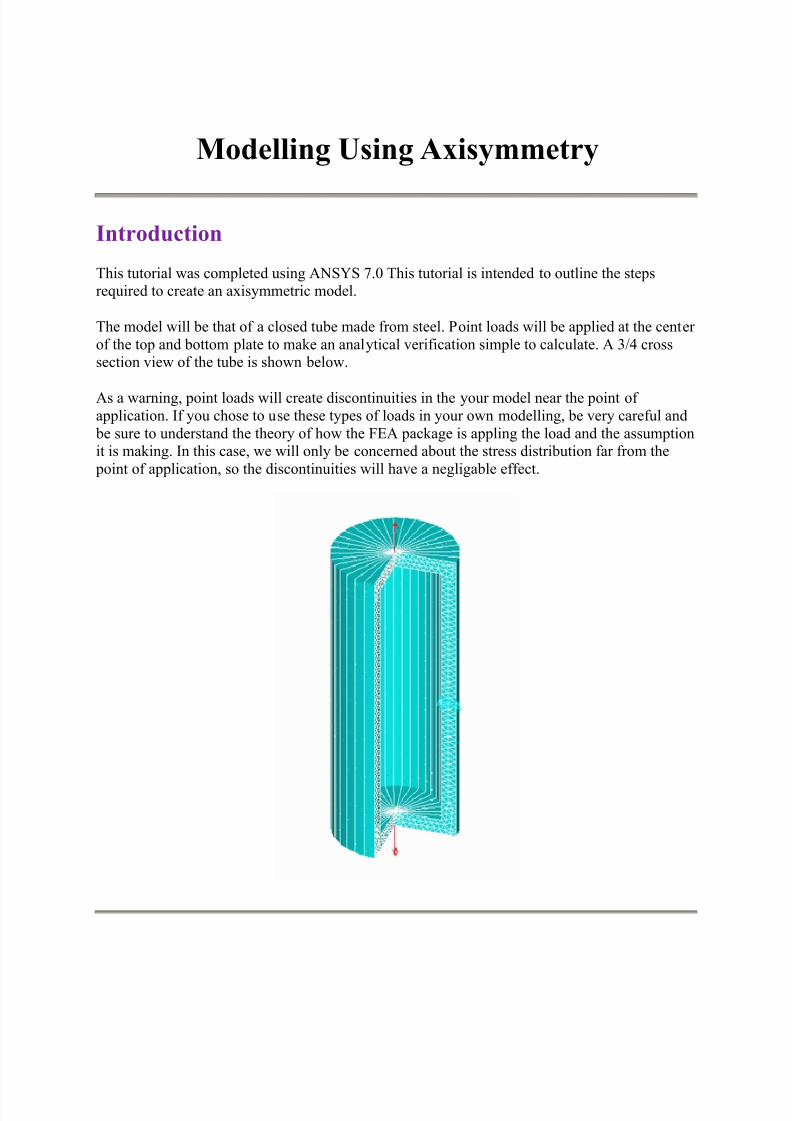
The model will be that of a closed tube made from steel. Point loads will be applied at the center

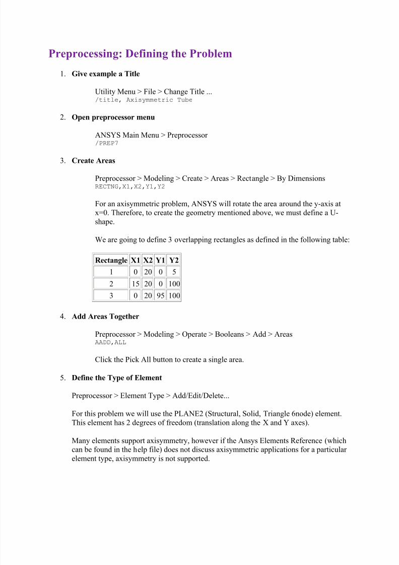
of the top and bottom plate to make an analytical verification simple to calculate. A 3/4 crosssection view of the tube is shown below.

As a warning, point loads will create discontinuities in the your model near the point of application. If you chose to use these types of loads in your own modelling, be very careful and

be sure to understand the theory of how the FEA package is appling the load and the assumptionit is making. In this case, we will only be concerned about the stress distribution far from the

point of application, so the discontinuities will have a negligable effect.



Preprocessing: Defining the Problem

1. Give example a Title

Utility Menu > File > Change Title ...

/title, Axisymmetric Tube

2. Open preprocessor menu

ANSYS Main Menu > Preprocessor /PREP7

3. Create Areas

Preprocessor > Modeling > Create > Areas > Rectangle > By DimensionsRECTNG,X1,X2,Y1,Y2

For an axisymmetric problem, ANSYS will rotate the area around the y-axis atx=0. Therefore, to create the geometry mentioned above, we must define a U-

shape.

We are going to define 3 overlapping rectangles as defined in the following table:

Rectangle X1 X2 Y1 Y2

1 0 20 0 5

2 15 20 0 100

3 0 20 95 100

4. Add Areas Together

Preprocessor > Modeling > Operate > Booleans > Add > AreasAADD,ALL

Click the Pick All button to create a single area.

5. Define the Type of Element

Preprocessor > Element Type > Add/Edit/Delete...

For this problem we will use the PLANE2 (Structural, Solid, Triangle 6node) element.

This element has 2 degrees of freedom (translation along the X and Y axes).

Many elements support axisymmetry, however if the Ansys Elements Reference (whichcan be found in the help file) does not discuss axisymmetric applications for a particular

element type, axisymmetry is not supported.



Turn on Axisymmetry

While the Element Types window is still open, click the Options... button.

Under Element behavior K3 select Axisymmetric.

Define Element Material Properties Preprocessor > Material Props > Material Models > Structural > Linear > Elastic >

Isotropic

In the window that appears, enter the following geometric properties for steel:

i. Young's modulus EX: 200000

ii. Poisson's Ratio PRXY: 0.3

Define Mesh Size

Preprocessor > Meshing > Size Cntrls > ManualSize > Areas > All Areas

For this example we will use an element edge length of 2mm.

Mesh the frame Preprocessor > Meshing > Mesh > Areas > Free > click 'Pick All'

Your model should know look like this:



Solution Phase: Assigning Loads and Solving

1. Define Analysis Type

Solution > Analysis Type > New Analysis > StaticANTYPE,0

Apply Constraints

Solution > Define Loads > Apply > Structural > Displacement > Symmetry B.C. > On

Lines

Pick the two edges on the left, at x=0, as shown below. By using the symmetry B.C.

command, ANSYS automatically calculates which DOF's should be constrained for theline of symmetry. Since the element we are using only has 2 DOF's per node, we could

have constrained the lines in the x-direction to create the symmetric boundary conditions.



Utility Menu > Select > Entities

Select Nodes and By Location from the scroll down menus. Click Y coordinates andtype 50 into the input box as shown below, then click OK.



Solution > Define Loads > Apply > Structural > Displacement > On Nodes > Pick All

Constrain the nodes in the y-direction (UY). This is required to constrain the model in

space, otherwise it would be free to float up or down. The location to constrain the modelin the y-direction (y=50) was chosen because it is along a symmetry plane. Therefore,

these nodes won't move in the y-direction according to theory.

Utility Menu > Select > Entities

In the select entities window, click Sele All to reselect all nodes. It is important to alwaysreselect all entities once you've finished to ensure future commands are applied to the whole

model and not just a few entities. Once you've clicked Sele All, click on Cancel to close the

window.

Apply Loads

Solution > Define Loads > Apply > Structural > Force/Moment > On Keypoints

Pick the top left corner of the area and click OK. Apply a load of 100 in the FY direction.

Solution > Define Loads > Apply > Structural > Force/Moment > On Keypoints

Pick the bottom left corner of the area and click OK. Apply a load of -100 in the FYdirection.

The applied loads and constraints should now appear as shown in the figure below.



Solve the System Solution > Solve > Current LSSOLVE

Postprocessing: Viewing the Results

1. Hand Calculations

Hand calculations were performed to verify the solution found using ANSYS:

The stress across the thickness at y = 50mm is 0.182 MPa.

2. Determine the Stress Through the Thickness of the Tube o Utility Menu > Select > Entities...



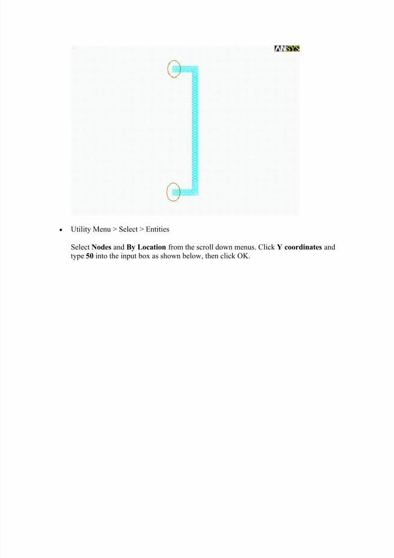
Select Nodes > By Location > Y coordinates and type 45,55 in the Min,Max box,as shown below and click OK.

o General Postproc > List Results > Nodal Solution > Stress > Components

SCOMP

The following list should pop up.



o If you take the average of the stress in the y-direction over the thickness of the

tube, (0.18552 + 0.17866)/2, the stress in the tube is 0.182 MPa, matching the

analytical solution. The average is used because in the analytical case, it isassumed the stress is evenly distributed across the thickness. This is only true

when the location is far from any stress concentrators, such as corners. Thus, to

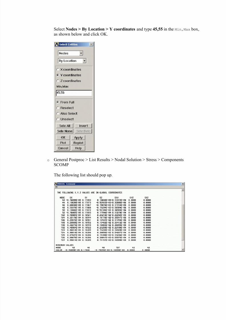
approximate the analytical solution, we must average the stress over the thickness.3. Plotting the Elements as Axisymmetric

Utility Menu > PlotCtrls > Style > Symmetry Expansion > 2-D Axi-symmetric...

The following window will appear. By clicking on 3/4 expansion you can

produce the figure shown at the beginning of this tutorial.

4. Extra Exercise

It is educational to repeat this tutorial, but leave out the key option which enables

axisymmetric modelling. The rest of the commands remain the same. If this is done, the

model is a flat, rectangular plate, with a rectangular hole in the middle. Both the stressdistribution and deformed shape change drastically, as expected due to the change in

geometry. Thus, when using axisymmetry be sure to verify the solutions you get are

reasonable to ensure the model is infact axisymmetric.

Data Plotting: Using Tables to Post Process

Results



Introduction

This tutorial was created using ANSYS 7.0 The purpose of this tutorial is to outline the steps

required to plot Vertical Deflection vs. Length of the following beam using tables, a special typeof array. By plotting this data on a curve, rather than using a contour plot, finer resolution can be

achieved.

This tutorial will use a steel beam 400 mm long, with a 40 mm X 60 mm cross section as shown

above. It will be rigidly constrained at one end and a -2500 N load will be applied to the other.

Preprocessing: Defining the Problem

1. Give the example a Title

Utility Menu > File > Change Title .../title, Use of Tables for Data Plots

2. Open preprocessor menu

ANSYS Main Menu > Preprocessor /PREP7

3. Define Keypoints

Preprocessor > Modeling > Create > Keypoints > In Active CS...K,#,x,y,z



We are going to define 2 keypoints for this beam as given in the following table:

Keypoint Coordinates (x,y,z)

1 (0,0)

2 (400,0)

4. Create Lines

Preprocessor > Modeling > Create > Lines > Lines > In Active CoordL,1,2

Create a line joining Keypoints 1 and 2

5. Define the Type of Element

Preprocessor > Element Type > Add/Edit/Delete...

For this problem we will use the BEAM3 (Beam 2D elastic) element. This element has 3degrees of freedom (translation along the X and Y axes, and rotation about the Z axis).

Define Real Constants Preprocessor > Real Constants... > Add...

In the 'Real Constants for BEAM3' window, enter the following geometric properties:

i. Cross-sectional area AREA: 2400

ii. Area moment of inertia IZZ: 320e3iii. Total beam height: 40

This defines a beam with a height of 40 mm and a width of 60 mm.

Define Element Material Properties Preprocessor > Material Props > Material Models > Structural > Linear > Elastic >

Isotropic

In the window that appears, enter the following geometric properties for steel:

i. Young's modulus EX: 200000ii. Poisson's Ratio PRXY: 0.3

Define Mesh Size Preprocessor > Meshing > Size Cntrls > ManualSize > Lines > All Lines...

For this example we will use an element edge length of 20mm.



Mesh the frame Preprocessor > Meshing > Mesh > Lines > click 'Pick All'

Solution Phase: Assigning Loads and Solving

1. Define Analysis Type

Solution > Analysis Type > New Analysis > StaticANTYPE,0

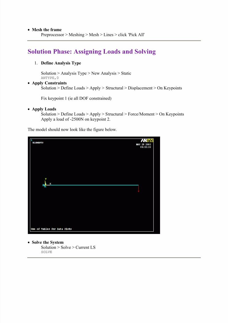
Apply Constraints Solution > Define Loads > Apply > Structural > Displacement > On Keypoints

Fix keypoint 1 (ie all DOF constrained)

Apply Loads

Solution > Define Loads > Apply > Structural > Force/Moment > On KeypointsApply a load of -2500N on keypoint 2.

The model should now look like the figure below.

Solve the System Solution > Solve > Current LSSOLVE



Postprocessing: Viewing the Results

It is at this point the tables come into play. Tables, a special type of array, are basically matrices

that can be used to store and process data from the analysis that was just run. This example is a

simplified use of tables, but they can be used for much more. For more information type help in

the command line and search for 'Array Parameters'.

1. Number of Nodes

Since we wish to plot the verticle deflection vs length of the beam, the location and

verticle deflection of each node must be recorded in the table. Therefore, it is necessaryto determine how many nodes exist in the model. Utility Menu > List > Nodes... > OK.

For this example there are 21 nodes. Thus the table must have at least 21 rows.

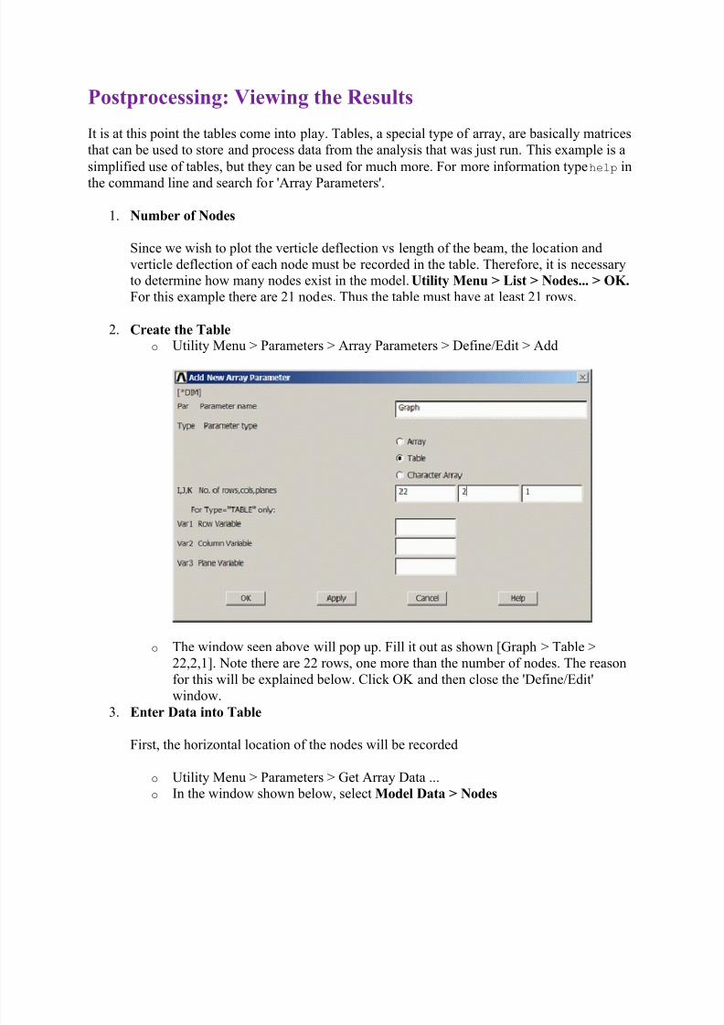
2. Create the Table o Utility Menu > Parameters > Array Parameters > Define/Edit > Add

o The window seen above will pop up. Fill it out as shown [Graph > Table >

22,2,1]. Note there are 22 rows, one more than the number of nodes. The reason

for this will be explained below. Click OK and then close the 'Define/Edit'

window.

3.

Enter Data into Table

First, the horizontal location of the nodes will be recorded

o Utility Menu > Parameters > Get Array Data ...o In the window shown below, select Model Data > Nodes



o Fill the next window in as shown below and click OK [Graph(1,1) > All >

Location > X]. Naming the array parameter 'Graph(1,1)' fills in the table startingin row 1, column 1, and continues down the column.

Next, the vertical displacement will be recorded.

o Utility Menu > Parameters > Get Array Data ... > Results data > Nodal resultso Fill the next window in as shown below and click OK [Graph(1,2) > All > DOF

solution > UY]. Naming the array parameter 'Graph(1,2)' fills in the table starting

in row 1, column 2, and continues down the column.



4. Arrange the Data for Ploting

Users familiar with the way ANSYS numbers nodes will realize that node 1 will be onthe far left, as it is keypoint 1, node 2 will be on the far right (keypoint 2), and the rest of

the nodes are numbered sequentially from left to right. Thus, the second row in the table

contains the data for the last node. This causes problems during plotting, thus theinformation for the last node must be moved to the final row of the table. This is why a

table with 22 rows was created, to provide room to move this data.

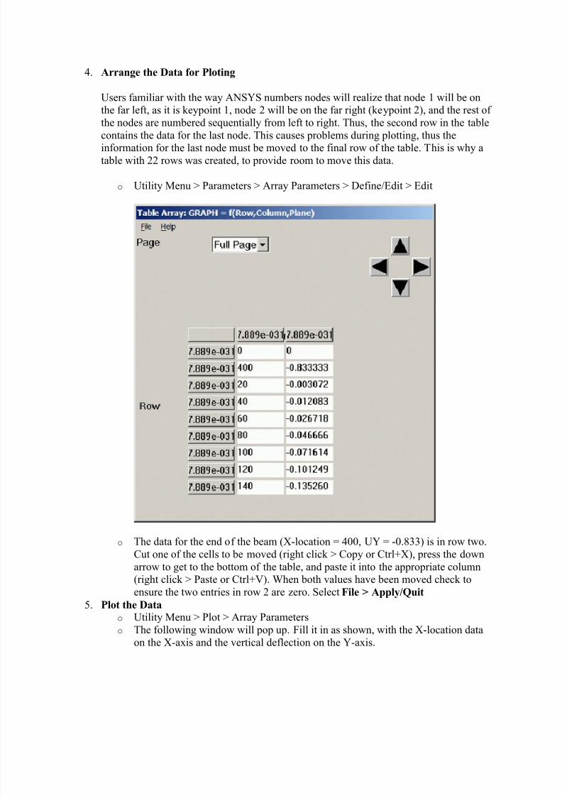
o Utility Menu > Parameters > Array Parameters > Define/Edit > Edit

o The data for the end of the beam (X-location = 400, UY = -0.833) is in row two.

Cut one of the cells to be moved (right click > Copy or Ctrl+X), press the downarrow to get to the bottom of the table, and paste it into the appropriate column(right click > Paste or Ctrl+V). When both values have been moved check to

ensure the two entries in row 2 are zero. Select File > Apply/Quit

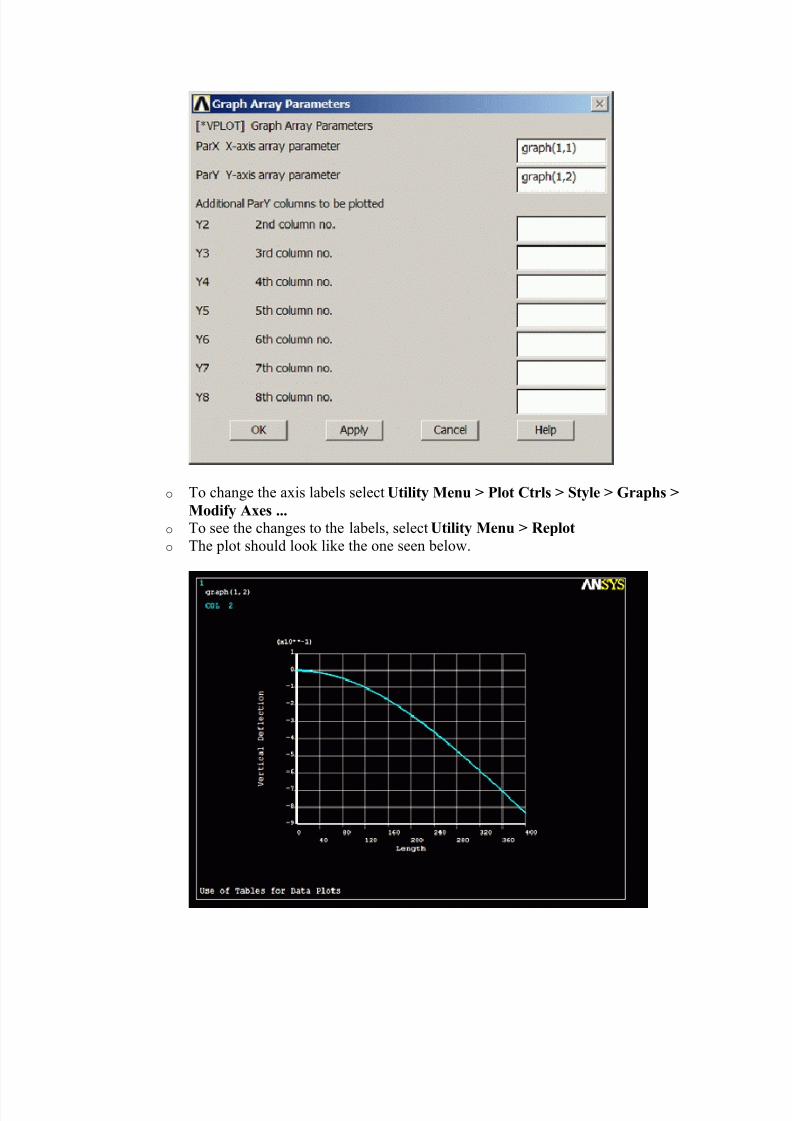
5. Plot the Data o Utility Menu > Plot > Array Parameters

o The following window will pop up. Fill it in as shown, with the X-location data

on the X-axis and the vertical deflection on the Y-axis.



o To change the axis labels select Utility Menu > Plot Ctrls > Style > Graphs >

Modify Axes ... o To see the changes to the labels, select Utility Menu > Replot o The plot should look like the one seen below.

ansys tutorialsintroduction.docx

Documents