The Cryosphere, 12, 1969–1985, 2018https://doi.org/10.5194/tc-12-1969-2018© Author(s) 2018. This work is distributed underthe Creative Commons Attribution 3.0 License.

Antarctic sub-shelf melt rates via PICORonja Reese1,3, Torsten Albrecht1, Matthias Mengel1, Xylar Asay-Davis1,2, and Ricarda Winkelmann1,3

1Potsdam Institute for Climate Impact Research (PIK), Member of the Leibniz Association, P.O. Box 60 12 03,14412 Potsdam, Germany2Los Alamos National Laboratory, P.O. Box 1663, T-3, MS-B216, Los Alamos, NM 87545, USA3University of Potsdam, Institute of Physics and Astronomy, Karl-Liebknecht-Str. 24-25, 14476 Potsdam, Germany

Correspondence: Ricarda Winkelmann (ricarda.winkelmann@pik-potsdam.de)

Received: 19 April 2017 – Discussion started: 27 June 2017Revised: 20 November 2017 – Accepted: 9 February 2018 – Published: 12 June 2018

Abstract. Ocean-induced melting below ice shelves is oneof the dominant drivers for mass loss from the AntarcticIce Sheet at present. An appropriate representation of sub-shelf melt rates is therefore essential for model simulationsof marine-based ice sheet evolution. Continental-scale icesheet models often rely on simple melt-parameterizations,in particular for long-term simulations, when fully coupledice–ocean interaction becomes computationally too expen-sive. Such parameterizations can account for the influenceof the local depth of the ice-shelf draft or its slope on melt-ing. However, they do not capture the effect of ocean circu-lation underneath the ice shelf. Here we present the PotsdamIce-shelf Cavity mOdel (PICO), which simulates the verti-cal overturning circulation in ice-shelf cavities and thus en-ables the computation of sub-shelf melt rates consistent withthis circulation. PICO is based on an ocean box model thatcoarsely resolves ice shelf cavities and uses a boundary layermelt formulation. We implement it as a module of the ParallelIce Sheet Model (PISM) and evaluate its performance underpresent-day conditions of the Southern Ocean. We identify aset of parameters that yield two-dimensional melt rate fieldsthat qualitatively reproduce the typical pattern of compara-bly high melting near the grounding line and lower meltingor refreezing towards the calving front. PICO captures thewide range of melt rates observed for Antarctic ice shelves,with an average of about 0.1 ma−1 for cold sub-shelf cavi-ties, for example, underneath Ross or Ronne ice shelves, to16 ma−1 for warm cavities such as in the Amundsen Sea re-gion. This makes PICO a computationally feasible and morephysical alternative to melt parameterizations purely basedon ice draft geometry.

1 Introduction

Dynamic ice discharge across the grounding lines into float-ing ice shelves is the main mass loss process of the AntarcticIce Sheet. Surrounding most of Antarctica’s coastlines, theice shelves themselves lose mass by ocean-induced meltingfrom below or calving of icebergs (Depoorter et al., 2013;Liu et al., 2015). Observations show that many Antarcticice shelves are thinning at present, driven by enhanced sub-shelf melting (Pritchard et al., 2012; Paolo et al., 2015).Thinning reduces the ice shelves’ buttressing potential, i.e.,the restraining force at the grounding line provided by theice shelves (Thomas, 1979; Dupont and Alley, 2005; Gud-mundsson et al., 2012), and can thereby accelerate upstreamglacier flow. The observed acceleration of tributary glaciersis seen as the major contributor to the current mass loss inthe West Antarctic Ice Sheet (Pritchard et al., 2012). In par-ticular, the recent dynamic ice loss in the Amundsen Seasector (MacGregor et al., 2012; Mouginot et al., 2014) isassociated with high melt rates that result from inflow ofrelatively warm circumpolar deep water (CDW) in the ice-shelf cavities (D. M. Holland et al., 2008; Jacobs et al., 2011;Pritchard et al., 2012; Schmidtko et al., 2014; Hellmer et al.,2017; Thoma et al., 2008). Also in East Antarctica, particu-larly at Totten glacier, as well as along the Southern Antarc-tic Peninsula, glacier thinning seems to be linked to CDWreaching the deep grounding lines (Greenbaum et al., 2015;Wouters et al., 2015). An appropriate representation of meltrates at the ice–ocean interface is hence crucial for simulat-ing the dynamics of the Antarctic Ice Sheet. Melting in ice-shelf cavities can occur in different modes that depend on theocean properties in the proximity of the ice shelf, the topog-

Published by Copernicus Publications on behalf of the European Geosciences Union.

1970 R. Reese et al.: Antarctic sub-shelf melt rates via PICO

raphy of the ocean bed and the ice-shelf subsurface (Jacobset al., 1992). Antarctica’s ice-shelf cavities can be classifiedinto “cold” and “warm” with typical mean melt rates rangingfrom O(0.1–1.0) m a−1 in “cold” cavities as for the Filchner-Ronne Ice-Shelf andO(10) ma−1 in “warm” cavities like theone adjacent to Pine Island Glacier (Joughin et al., 2012).For the “cold” cavities of the large Ross, Filchner-Ronne andAmery ice shelves, freezing to the shelf base is observed inthe shallower areas near the center of the ice shelf and to-wards the calving front (Rignot et al., 2013; Moholdt et al.,2014).

Since the stability of the ice sheet is strongly linked tothe dynamics of the buttressing ice shelves, it is essentialto adequately represent their mass balance. A number ofparameterizations with different levels of complexity havebeen developed to capture the effect of sub-shelf melting.Simplistic parameterizations that depend on the local oceanand ice-shelf properties have been applied in long-term andlarge-scale ice sheet simulations (Joughin et al., 2014; Martinet al., 2011; Pollard and DeConto, 2012; Favier et al., 2014).These parameterizations make melt rates piece-wise linearfunctions of the depth of the ice-shelf draft (Beckmann andGoosse, 2003) or of the slope of the ice-shelf base (Littleet al., 2012). Other models describe the evolution of melt-water plumes forming at the ice-shelf base (Jenkins, 1991).Plumes evolve depending on the ice-shelf draft and slope,sub-glacial discharge and entrainment of ambient ocean wa-ter. This approach has been applied to models with charac-teristic conditions for Antarctic ice shelves (Holland et al.,2007; Payne et al., 2007; Lazeroms et al., 2018) and forGreenland outlet glaciers and fjord systems (Jenkins, 2011;Carroll et al., 2015; Beckmann et al., 2018). Interactivelycoupled ice–ocean models that resolve both the ice flow andthe water circulation below ice shelves are now becomingavailable (Goldberg et al., 2012; Thoma et al., 2015; Seroussiet al., 2017; De Rydt and Gudmundsson, 2016). There is acommunity effort to better understand effects of ice–oceaninteraction in such coupled models (Asay-Davis et al., 2016).However, as ocean models have many more degrees of free-dom than ice sheet models and require for much shorter timesteps, coupled simulations are currently limited to short timescales (on the order of decades to centuries).

Here, we present the Potsdam Ice-shelf Cavity mOdel(PICO), which provides sub-shelf melt rates in a computa-tionally efficient manner and accounts for the basic verticaloverturning circulation in ice-shelf cavities driven by the icepump (Lewis and Perkin, 1986). It is based on the earlierwork of Olbers and Hellmer (2010) and is implemented as amodule in the Parallel Ice Sheet Model (PISM: Bueler andBrown, 2009; Winkelmann et al., 2011).1 Ocean temperatureand salinity at the depth of the bathymetry in the continentalshelf region serve as input data. PICO allows for long-termsimulations (on centennial to millennial time scales) and for

1http://www.pism-docs.org (last access: 15 May 2018)

large ensembles of simulations which makes it applicable,for example, in paleo-climate studies or as a coupling mod-ule between ice-sheet and Earth System models.

In this paper, we give a brief overview of the cavity circu-lation and melt physics and describe the ocean box geometryin PICO and implementation in PISM in Sect. 2. In Sect. 3,we derive a valid parameter range for present-day Antarcticaand compare the resulting sub-shelf melt rates to observa-tional data. This is followed by a discussion of the applica-bility and limitations of the model (Sect. 4) and conclusions(Sect. 5).

2 Model description

PICO is developed from the ocean box model of Olbers andHellmer (2010), henceforth referred to as OH10. The OH10model is designed to capture the basic overturning circulationin ice-shelf cavities which is driven by the “ice pump” mech-anism: melting at the ice-shelf base near the grounding linereduces salinity and the ambient ocean water becomes buoy-ant, rising along the ice-shelf base towards the calving front.Since the ocean temperatures on the Antarctic continentalshelf are generally close to the local freezing point, densityvariations are primarily controlled by salinity changes. Melt-ing at the ice-shelf base hence reduces the density of ambientwater masses, resulting in a haline driven circulation. Buoy-ant water rising along the shelf base draws in ocean water atdepth, which flows across the continental shelf towards thedeep grounding lines of the ice shelves. The warmer thesewater masses are, the stronger the melting-induced ice pumpwill be. The OH10 box model describes the relevant physicalprocesses and captures this vertical overturning circulationby defining consecutive boxes following the flow within theice-shelf cavity. The strength of the overturning flux q is de-termined from the density difference between the incomingwater masses on the continental shelf and the buoyant watermasses near the deep grounding lines of the ice shelf.

As PICO is implemented in an ice sheet model with char-acteristic time scales much slower than typical responsetimes of the ocean, we assume steady state ocean conditionsand hence reduce the complexity of the governing equationsof the OH10 model. Using this assumption facilitates adap-tive box adjustment to grounding line migration, especiallysince PICO transfers the box model approach into two hor-izontal dimensions. We assume stable vertical stratification;OH10 found that a circulation state for an unstable verticalwater column, which would imply a high (parametrized) dif-fusive transport between boxes, only occurs transiently (Ol-bers and Hellmer, 2010, Sect. 2). This motivates neglectingthe diffusive heat and salt transport between boxes whichis small under these conditions. Without diffusive transportbetween the boxes, some of the original ocean boxes fromOH10 become passive and can be incorporated into the gov-erning equations of the set of boxes used in PICO. We

The Cryosphere, 12, 1969–1985, 2018 www.the-cryosphere.net/12/1969/2018/

R. Reese et al.: Antarctic sub-shelf melt rates via PICO 1971

Table 1. PICO parameters and typical values.

Parameter Symbol Value Unit

Salinity coefficient of freezing equation a −0.0572 ◦C PSU−1

Constant coefficient of freezing equation b 0.0788 ◦CPressure coefficient of freezing equation c 7.77× 10−8 ◦C Pa−1

Thermal expansion coefficient in EOS α 7.5× 10−5 ◦C−1

Salt contraction coefficient in EOS β 7.7× 10−4 PSU−1

Reference density in EOS ρ∗ 1033 kgm−3

Latent heat of fusion L 3.34× 105 Jkg−1

Heat capacity of sea water cp 3974 Jkg−1 ◦C−1

Density of ice ρi 910 kgm−3

Density of sea water ρw 1028 kgm−3

Turbulent salinity exchange velocity γS 2× 10−6 ms−1

Turbulent temperature exchange velocity γT 5× 10−5 ms−1

Effective turbulent temperature exchange velocity γ ∗T 2× 10−5 ms−1

Overturning strength C 1× 106 m6 s−1 kg−1

The coefficients in the equation of state (EOS), the turbulent exchange velocities for heat and salt, are taken from Olbers andHellmer (2010). We linearized the potential freezing temperature equation with a least-squares fit with salinity values over arange of 20–40 PSU and pressure values of 0–107 Pa using Gibbs SeaWater Oceanographic Package of TEOS-10(McDougall and Barker, 2011). All values are kept constant, except for γ ∗T and C, which vary between experiments. Thevalues of these two parameters are the best-fit from Sect. 3.1.

explicitly model a single open ocean box which providesthe boundary conditions for the boxes adjacent to the ice-shelf base following the overturning circulation, as shown inFig. 1. In order to better resolve the complex melt patterns,PICO adapts the number of boxes based on the evolving ge-ometry of the ice shelf. These simplifying assumptions allowus to analytically solve the system of governing equations,which is presented in the following two sections. A detailedderivation of the analytic solutions is given in Appendix A.In Sect. 2.3, we describe how the ice-model grid relatesto the ocean box geometry of PICO. The system of equa-tions is solved locally on the ice-model grid, as described inSect. 2.4. Table 1 summarizes the model parameters and typ-ical values.

2.1 Physics of the overturning circulation in ice-shelfcavities

PICO solves for the transport of heat and salt between theocean boxes as depicted in Fig. 1. Although box B0, whichis located at depth between the ice-shelf front and the edgeof the continental shelf, does not extend into the shelf cavity,its properties are transported unchanged from box B0 to boxB1 near the grounding line. The heat and salt balances forall boxes in contact with the ice-shelf base (boxes Bk for k ∈{1, . . .n}) can be written as

VkTk = qTk−1− qTk +AkmkTbk −AkmkTk

+AkγT (Tbk − Tk) , (1)VkSk = qSk−1− qSk +AkmkSbk −AkmkSk

+AkγS (Sbk − Sk) . (2)

n

Ice sheet Ice shelf

Grounding line

Figure 1. Schematic view of the PICO model. The model mimicsthe overturning circulation in ice-shelf cavities: ocean water frombox B0 enters the ice-shelf cavity at the depth of the sea floor andis advected to the grounding line box B1. Freshwater influx frommelting at the ice-shelf base makes the water buoyant, causing itto rise. The cavity is divided into n boxes along the ice-shelf base.Generally, the highest melt rates can be found near the groundingline, with lower melt rates or refreezing towards the calving front.

The local application of these equations for each ice modelcell is described in Sect. 2.4. Since we assume steady circu-lation, the terms on the left-hand side are neglected. For theboxBk with volume Vk , heat or salt content change due to ad-vection from the adjacent box Bk−1 with overturning flux q(first term on the right-hand side) and due to advection to theneighboring box Bk+1 (or the open ocean for k = n; secondterm). Vertical melt flux into the box Bk across the ice–ocean

www.the-cryosphere.net/12/1969/2018/ The Cryosphere, 12, 1969–1985, 2018

1972 R. Reese et al.: Antarctic sub-shelf melt rates via PICO

interface with area Ak (third term) and out of the box (fourthterm) play a minor role and are neglected in the analytic so-lution of the equation system employed in PICO (a detaileddiscussion of these terms is given in Jenkins et al., 2001). Themelt rate mk is negative if ambient water freezes to the shelfbase. The last term represents heat and salt changes via turbu-lent, vertical diffusion across the boundary layer beneath theice–ocean interface. The parameters γT and γS are the tur-bulent heat and salt exchange velocities which we assume,following OH10, to be constant.

The overturning flux q > 0 is assumed to be driven by thedensity difference between the ocean reservoir box B0 andthe grounding line box B1. This is parametrized as in OH10as

q = C (ρ0− ρ1) , (3)

where C is a constant overturning coefficient that captureseffects of friction, rotation and bottom form stress.2 The cir-culation strength in PICO is hence determined by densitychanges through sub-shelf melting in the grounding zone boxB1. From there, water follows the ice-shelf base towards theopen ocean assuming the overturning flux q to be the samefor all subsequent boxes. Ocean water densities are computedassuming a linear approximation of the equation of state:

ρ = ρ∗ (1−α (T − T∗)+β (S− S∗)) , (4)

where T∗ = 0 ◦C, S∗ = 34 PSU and α, β and ρ∗ are constantswith values given in Table 1.

2.2 Melting physics

Melting physics are derived from the widely used 3-equationmodel (Hellmer and Olbers, 1989; Holland and Jenkins,1999), which assumes the presence of a boundary layer be-low the ice–ocean interface. The temperature at this interfacein box Bk is assumed to be at the in situ freezing point Tbk ,which is linearly approximated by

Tbk = a Sbk + b− cpk, (5)

where pk is the overburden pressure, here calculated asstatic-fluid pressure given by the weight of the ice on top.At the ice–ocean interface, the heat flux from the ambientocean across the boundary layer due to turbulent mixing,QT = ρwcpγT (Tbk − Tk), equals the heat flux due to meltingor freezingQTb =−ρiLmk . Neglecting heat flux into the ice,the heat balance equation thus reads

γT (Tbk − Tk)=−νλmk, (6)

where ν = ρi/ρw ∼ 0.89, λ= L/cp ∼ 84 ◦C. We obtain thesalt flux boundary condition as the balance between tur-bulent salt transfer across the boundary layer, QS =

2For a more detailed discussion see Olbers and Hellmer (2010,Sect. 2).

ρwγS (Sbk − Sk), and reduced salinity due to melt water in-put, QSb =−ρiSbkmk ,

γS (Sbk − Sk)=−νSbkmk. (7)

To compute melt rates, we apply a simplified version of the 3-equations model (McPhee, 1992, 1999; Holland and Jenkins,1999) which allows for a simple, analytic solution of the sys-tem of governing equations. It has been shown that this for-mulation yields realistic heat fluxes (McPhee, 1992, 1999).This simplification is used only for melt rates, we neverthe-less solve for the boundary layer salinity which is central tothe solution of the system of equations as detailed in Ap-pendix A. Melt rates are given by

mk =−γ ∗Tνλ(aSk + b− cpk − Tk) , (8)

with ambient ocean temperature Tk and salinity Sk in boxBk . Here, we use the effective turbulent heat exchange coef-ficient γ ∗T . The relation between γT and γ ∗T is discussed in theAppendix A.

2.3 PICO ocean box geometry

PICO is implemented as a module in the three-dimensionalice sheet model PISM as described in Sect. 2.4. Since theoriginal system of box-model equations is formulated foronly one horizontal and one vertical dimension, it needed tobe extended for the use in the three-dimensional ice sheetmodel. The system of governing equations as described inthe previous two sections is solved for each ice shelf inde-pendently. PICO adapts the ocean boxes to the evolving iceshelves at every time step.

For any shelf D, we determine the number of ocean boxesnD by interpolating between 1 and nmax depending on its sizeand geometry such that larger ice shelves are resolved withmore boxes. The maximum number of boxes nmax is a modelparameter; a value of 5 is suitable for the Antarctic setup, asdiscussed further in Sect. 3.2. We determine the number ofboxes nD for each individual ice shelf D with

nD = 1+ rd(√dGL(D)/dmax (nmax− 1)

), (9)

where rd( ) rounds to the nearest integer. Here, dGL(x,y) isthe local distance to the grounding line from an ice-modelgrid cell with horizontal coordinates (x, y), dGL(D) is themaximum distance within ice shelf D and dmax is the maxi-mum distance to the grounding line within the entire compu-tational domain.

Knowing the maximum number of boxes nD for an iceshelf D, we next define the ocean boxes underneath it. Theextent of boxes B1, . . .,BnD is determined using the dis-tance to the grounding line and the shelf front. The non-dimensional relative distance to the grounding line r is de-fined as

r (x,y)= dGL (x,y)/(dGL (x,y)+ dIF (x,y)) , (10)

The Cryosphere, 12, 1969–1985, 2018 www.the-cryosphere.net/12/1969/2018/

R. Reese et al.: Antarctic sub-shelf melt rates via PICO 1973

with dIF (x,y) the horizontal distance to the ice front. Weassign all ice cells with horizontal coordinates (x,y) ∈D tobox Bk if the following condition is met:

1−√(nD − k+ 1)/nD ≤ r (x,y)≤ 1−

√(nD − k)/nD . (11)

This leads to comparable areas for the different boxes withina shelf, which is motivated in Appendix B. Thus, for exam-ple, the box B1 adjacent to the grounding line interacts withall ice shelf grid cells with 0≤ r ≤ 1−

√(nD − 1)/nD . Fig-

ure 3 shows an example of the ocean box areas for Antarc-tica. PICO does currently not account for melting along verti-cal ice cliffs, as, for example, the termini of some Greenlandoutlet fjords.

2.4 Implementation in the Parallel Ice Sheet Model

PICO is implemented in the open-source Parallel Ice SheetModel (PISM: Bueler and Brown, 2009; Winkelmann et al.,2011). In the three-dimensional, thermo-mechanically cou-pled, finite-difference model, ice velocities are computedthrough a superposition of the shallow approximations forthe slow, shear-dominated flow in ice sheets (Hutter, 1983,SIA) and the fast, membrane-like flow in ice streams andice shelves (Morland, 1987, SSA). In PISM, the groundinglines (diagnosed via the flotation criterion) and ice frontsevolve freely. Grounding line movement has been evalu-ated in the model intercomparison project MISMIP3d (Pat-tyn et al., 2013; Feldmann et al., 2014).

PICO is synchronously coupled to the ice-sheet model,i.e., they use the same adaptive time steps. The cavity modelprovides sub-shelf melt rates and temperatures at the ice–ocean boundary to PISM, with temperatures being at the insitu freezing point. PISM supplies the evolving ice-shelf ge-ometry to PICO, which in turn adjusts in each time step theocean box geometry to the ice-shelf geometry as describedin Sect. 2.3.

PICO computes the melt rates progressively over the oceanboxes, independently for each ice shelf. Since the ice-sheetmodel has a much higher resolution, each ocean box inter-acts with a number of ice-shelf grid cells. PICO applies theanalytic solutions of the system of governing equations sum-marized in Sect. 2.1 and 2.2 locally to the ice model grid asdetailed below. Model parameters that are varied between theexperiments are the effective turbulent heat exchange veloc-ity γ ∗T from the melt parametrization described in Sect. 2.2and the overturning coefficient C described in Sect. 2.1. Thetwo parameter values are applied to the entire ice sheet.

Input for PICO in the ocean reservoir box B0 is data fromobservations or large-scale ocean models in front of the iceshelves. Temperature T0 and salinity S0 are averaged at thedepth of the bathymetry in the continental shelf region. Inbox B1 adjacent to the grounding line, PICO solves the sys-tem of governing equations in each ice grid cell (x, y) to at-tain the overturning flux q (x,y), temperature T1 (x,y), salin-ity S1 (x,y), and the melting m1 (x,y) at its ice–ocean inter-

face (given by the local solution of Eqs. 3, A12, A8 and 8, re-spectively). The model proceeds progressively from box Bkto box Bk+1 to solve for sub-shelf melt rate mk+1 (x,y), am-bient ocean temperature Tk+1 (x,y), and salinity Sk+1 (x,y)

(given by the local solution of Eqs. 13, A13 and A8, respec-tively) based on the previous solutions Sk and Tk in box Bkand conditions at the ice–ocean interface. PICO provides theboundary conditions Tk and Sk to box Bk+1 as the averageover the ice-grid cells within box Bk , i.e.,

Tk = 〈Tk (x,y) with (x,y) in Bk〉 (12)

and analogously for Sk , where 〈 〉 denotes the average.The overturning is solved in Box B1 and given by q =〈q (x,y) with (x,y) in B1〉. Melt rates in box Bk are com-puted using the local overburden pressure pk (x,y) in eachice-shelf grid cell that is given by the weight of the ice col-umn provided by PISM, i.e.,

mk (x,y)=−γ ∗Tνλ(aSk (x,y)+ b− cpk (x,y)− Tk (x,y)) . (13)

This reflects the pressure dependence of heat available formelting and leads to a depth-dependent melt rate patternwithin each box. The implications for energy and mass con-servation are discussed in Sects. 3.2 and 4.

3 Results for present-day Antarctica

We apply PICO to compute sub-shelf melt rates for allAntarctic ice shelves under present-day conditions. Oceanicinput for each ice shelf is given by observations of temper-ature (converted to potential temperature) and salinity (con-verted to practical salinity) of the water masses occupying thesea floor on the continental shelf (Schmidtko et al., 2014),averaged over the time period 1975 to 2012. Water masseswithin an ice-shelf cavity originate from source regions: ne-glecting ocean dynamics, we approximate these by averagingocean properties on the depth of the continental shelf withinregions that are chosen to encompass areas of similar, large-scale ocean conditions. Oceanic input is given for 19 basinsof the Antarctic Ice Sheet, which are based on Zwally et al.(2012) and extended to the attached ice shelves and the sur-rounding Southern Ocean (Fig. 2). For each ice shelf, tem-perature T0 and salinity S0 in box B0 are obtained by av-eraging the basin input weighted with the fractional area ofthe shelf within the corresponding basin. Figure 2 shows thebasin-mean ocean temperature (shadings and numbers) andsalinity (numbers) used.3

Here, we use nmax = 5 from which PICO determines thenumber of ocean boxes in each shelf via Eq. (9). Figure 3

3We combine drainage sectors feeding the same ice shelf, e.g.,all contributory inlets to Filchner-Ronne or Ross Ice Shelves. Wealso consolidate the basins “IceSat21” and “IceSat22” (Pine IslandGlacier and Thwaites Glacier) as well as “IceSat7” and “IceSat8”in East Antarctica.

www.the-cryosphere.net/12/1969/2018/ The Cryosphere, 12, 1969–1985, 2018

1974 R. Reese et al.: Antarctic sub-shelf melt rates via PICO

1

23

4

5

6

7

8

9

10

11

1213

1415

16

1718

19

-1.76 °C34.82 psu

-1.66 °C34.70 psu

-1.65 °C34.48 psu -1.58 °C

34.49 psu

-1.51 °C34.5 psu

-1.73 °C34.70 psu

-1.68 °C34.65 psu

-0.73 °C34.73 psu

-1.61 °C34.75 psu

-1.30 °C34.84 psu

-1.83 °C34.95 psu

-1.58 °C34.79 psu

-0.36 °C34.58 psu

0.47 °C34.73 psu

1.04 °C34.86 psu

1.17 °C34.84 psu

0.23 °C34.70 psu -1.23 °C

34.76 psu

-1.80 °C34.84 psu

Tem

pera

ture

(°C

)

Figure 2. PICO input for Antarctic basins. The ice sheet, ice shelves and the surrounding Southern Ocean are split into 19 basins thatare based on Zwally et al. (2012) and indicated by black contour lines and labels. For each ice shelf, the governing equations are solvedseparately with the respective oceanic boundary conditions. For ice shelves that cross basin boundaries, the input is averaged, weighted withthe fractional area of the shelf within the corresponding basin. Numbers show the temperature and salinity input in each basin, obtained byaveraging observed properties of the ocean water in front of the ice-shelf cavities at depth of the continental shelf (Schmidtko et al., 2014),indicated by the color shading. Grey lines show Antarctic grounding lines and ice-shelf fronts (Fretwell et al., 2013).

displays the resulting extent of the ocean boxes for Antarc-tica, ordered in elongated bands beneath the ice shelves. Forthe large ice-shelf cavities of Filchner-Ronne and Ross, theice–ocean boundary is divided into five ocean boxes whilesmaller ice shelves have two to four boxes (see Table 2). In-troducing more than five ocean boxes has a negligible effecton the melt rates, as discussed in Sect. 3.2.

To validate our model, we run diagnostic simulations withPISM+PICO based on bed topography and ice thicknessfrom BEDMAP2 (Fretwell et al., 2013), mapped to a gridwith 5 km horizontal resolution. Diagnostic simulations al-low us to assess the sensitivity of the model to the parametersC and γ ∗T and to the number of boxes nmax as well as the icemodel resolution. Transient behavior is exemplified in a sim-ulation starting from an equilibrium state of the Antarctic Ice

Sheet forced with ocean temperature changes, see Video S1in the Supplement and Sect. 3.3.

3.1 Sensitivity to model parameters C and γ ∗T

We test the sensitivity of sub-shelf melt rates to the modelparameters for overturning strength C ∈ [0.1, 9]Svm3 kg−1

and the effective turbulent heat exchange velocity γ ∗T ∈ [5×10−6, 1× 10−4

]ms−1. These ranges encompass the valuesidentified in OH10, discussed further in Appendix A. Thesame parameters for C and γ ∗T are applied to all shelves. Weconstrain the results by the following qualitative criteria (1)and (2), as well as the quantitative constraints (3) and (4),summarized in Fig. 4:

Criterion (1). Freezing must not occur in the first box B1of any ice shelf, i.e., the ocean box closest to the ground-

The Cryosphere, 12, 1969–1985, 2018 www.the-cryosphere.net/12/1969/2018/

R. Reese et al.: Antarctic sub-shelf melt rates via PICO 1975

180◦150◦W 150◦E

60◦S

60◦S

1000km

B1

B2

B3

B4

B5

Figure 3. Extent of PICO ocean boxes for Antarctic ice shelves. Most ice shelves are split into two, three, or four ocean boxes interactingwith the ice cells on a much higher resolution. The largest ice shelves, Filchner-Ronne and Ross, have five ocean boxes. One ocean boxtypically corresponds to many ice-shelf grid cells.

Table 2. Results from the reference simulation as displayed in Fig. 5.

Ice-shelf bn T0 S0 Tn Sn 1T 1S q m mobserved

Larsen C 3 −1.33 34.60 −2.02 34.28 −0.69 −0.32 0.16 0.76 0.45 ± 1.00Wilkins, Stange, Bach, George VI 4 1.17 34.67 −1.41 33.48 −2.58 −1.19 0.32 9.50 1.46 ± 1.00Pine Island 2 0.46 34.55 −0.49 34.12 −0.94 −0.44 0.17 16.15 16.20 ± 1.00Thwaites 2 0.46 34.55 −0.62 34.06 −1.07 −0.50 0.13 14.55 17.73 ± 1.00Getz 3 −0.37 34.41 −1.63 33.83 −1.26 −0.58 0.23 7.04 4.26 ± 0.40Drygalski 3 −1.84 34.78 −2.03 34.69 −0.19 −0.09 0.02 0.69 3.27 ± 0.50Cook 2 −1.62 34.58 −1.94 34.43 −0.32 −0.15 0.05 2.63 1.33 ± 1.00Ninnis 2 −1.62 34.58 −1.88 34.45 −0.26 −0.12 0.04 3.63 1.17 ± 2.00Mertz 3 −1.62 34.58 −1.99 34.40 −0.38 −0.17 0.04 1.46 1.43 ± 0.60Totten 2 −0.68 34.57 −1.26 34.29 −0.59 −0.27 0.13 9.90 10.47 ± 0.70Shackleton 3 −1.69 34.48 −2.03 34.32 −0.34 −0.16 0.07 0.42 2.78 ± 0.60West 2 −1.69 34.48 −2.01 34.33 −0.32 −0.15 0.07 1.17 1.74 ± 0.70Amery 3 −1.72 34.53 −2.16 34.33 −0.43 −0.20 0.16 0.55 0.58 ± 0.40Baudouin 3 −1.55 34.33 −2.06 34.09 −0.51 −0.23 0.12 0.50 0.43 ± 0.40Fimbul 3 −1.57 34.32 −2.06 34.10 −0.49 −0.23 0.10 0.56 0.57 ± 0.20Riiser-Larsen 3 −1.66 34.53 −2.06 34.34 −0.40 −0.19 0.09 0.43 0.20 ± 0.20Stancomb, Brunt 3 −1.66 34.53 −2.01 34.37 −0.35 −0.16 0.08 0.35 0.03 ± 0.20Filchner-Ronne 5 −1.76 34.65 −2.19 34.45 −0.43 −0.20 0.21 0.06 0.32 ± 0.10Ross 5 −1.58 34.63 −2.12 34.38 −0.53 −0.25 0.17 0.06 0.10 ± 0.10

The number of boxes for each is ice-shelf is given by bn, T0 (S0) is the temperature (salinity) in ocean box B0, Tn (Sn) the temperature (salinity) averaged over the oceanbox at the ice-shelf front, 1T = Tn − T0 and 1S = Sn − S0. m is the average sub-shelf melt rate, mobserved the observed melt rates from Rignot et al. (2013). q is theoverturning flux. Unit of temperatures is ◦C, salinity is given in PSU, melt rates in m a−1 and overturning flux in Sv.

www.the-cryosphere.net/12/1969/2018/ The Cryosphere, 12, 1969–1985, 2018

1976 R. Reese et al.: Antarctic sub-shelf melt rates via PICO

0.6 0.8 1.0 3.0 5.0 7.0 9.0

0.2

0.4

0.6

0.8

1.0

3.0

5.0

7.0

9.0

Over

turn

ing

coeffi

cien

tC

m >1 0

0.6 0.8 1.0 3.0 5.0 7.0 9.0

Heat exchange coefficientγ∗T (×10−5 m s−1)

0.2

0.4

0.6

0.8

1.0

3.0

5.0

7.0

9.0

Over

turn

ing

coeffi

cien

tC

(Sv m

kg

)

m1 ≥ m2

0.6 0.8 1.0 3.0 5.0 7.0 9.0

0.2

0.4

0.6

0.8

1.0

3.0

5.0

7.0

9.0

FRIS (basin 1)

-0.2

0.0

0.2

0.4

0.6

0.8

Aver

age

mel

tra

te(m

a−

1)

0.6 0.8 1.0 3.0 5.0 7.0 9.0

Heat exchange coefficientγ∗T (×10−5 m s−1)

0.2

0.4

0.6

0.8

1.0

3.0

5.0

7.0

9.0

PIG (basin 14)

20.0

40.0

60.0

80.0

Aver

age

mel

tra

te(m

a−

1)

(a) (c)

(b) (d)

-13

(Sv m

kg

)-1

3

Figure 4. Sensitivity of PICO sub-shelf melt rates to the overturning coefficient C and the effective turbulent heat exchange coefficientγ ∗T . Black contour indicates the valid range of parameters, all other parameter combinations are excluded by one of the following criteria:no freezing may occur in the first ocean box (a), mean basal melt rates must decrease between the first and second ocean box (b). Greencontour indicates the valid range of parameters where the following quantitative constraints are additionally met: mean basal melt rates forFilchner-Ronne Ice Shelf should be within the range of 0.01 to 1.0 ma−1 (c), mean basal melt rates for Pine Island Glacier Ice Shelf shouldbe within the range of 10.0 to 25.0 ma−1 (d). The best-fit parameters (brown contour) minimize the root-mean-square error of mean meltrates to observations for both ice shelves.

ing line. Freezing in box B1 would increase ambient salinity,and since the overturning circulation in ice-shelf cavities ismainly haline driven, the circulation would shut down, vio-lating the model assumption q > 0 (see Sect. 2). As shownin Fig. 4a, the condition is not met for a combination of rel-atively high turbulent heat exchange and relatively low over-turning parameters. In such cases, freezing near the ground-ing line occurs because of the strong heat exchange betweenthe ambient ocean and the ice–ocean boundary in box B1 thatcannot be balanced by the resupply of heat from the openocean through overturning.

Criterion (2). Sub-shelf melt rates must decrease betweenthe first and second box for each ice shelf. This condition isbased on general observations of melt-rate patterns and onthe assumption that ocean water masses move consecutivelythrough the boxes and cool down along the way, as longas melting in these boxes outweighs freezing. As shown inFig. 4b, this condition is violated for either high overturningand low turbulent heat exchange or, vice versa, low overturn-ing and high turbulent heat exchange. An appropriate balancebetween the strength of these values is hence necessary for arealistic melt rate pattern.

If criterion (1) or (2) fails, basic assumptions of PICO areviolated. Thus, we choose the model parameters γ ∗T and Csuch that both criteria are strictly met. The following quan-titative, observational constraints (3) and (4) compare mod-eled average melt rates with observations and thus dependon our choice of valid ranges. We choose Filchner-Ronne IceShelf and the ice shelf adjacent to Pine Island Glacier to fur-ther constrain our model parameters for Antarctica. Theseshelves represent two different types regarding both the modeof melting and the ice-shelf size.

Observational constraint (3). Average melt rates inFilchner-Ronne Ice Shelf comply with the classification ofa “cold” cavity and lie between 0.01 and 1.0 ma−1 (Fig. 4c).

Observational constraint (4). For Pine Island Glacier, with“warm” ocean conditions, average melt rates lie between 10and 25 ma−1 (Fig. 4d).

Generally, an increase in overturning strength C will sup-ply more heat and thus yield higher melt rates, especiallyfor the large and “cold” ice shelves like Filchner-Ronne.Larger C leads to higher melt rates also in the smaller and“warm” Pine-Island Glacier Ice Shelf but the effect is lesspronounced. In contrast, the turbulent heat exchange alters

The Cryosphere, 12, 1969–1985, 2018 www.the-cryosphere.net/12/1969/2018/

R. Reese et al.: Antarctic sub-shelf melt rates via PICO 1977

Figure 5. Sub-shelf melt rates for present-day Antarctica computed with PISM+PICO. The mean melt rate per ice shelf (upper numbers) iscompared to the observed melt rates (lower numbers with uncertainty ranges) from Rignot et al. (2013). In the model, the same parametersγ ∗T = 2×10−5 ms−1 and C = 1 Svm3 kg−1 are applied to all ice shelves around Antarctica. The respective oceanic boundary condition areshown in Fig. 2. Ice geometry and bedrock topography are from the BEDMAP2 data set on 5 km resolution (Fretwell et al., 2013). Refreezingoccurs in some parts of the larger shelves like Filchner-Ronne and Ross.

melting, particularly in small ice shelves, while it might de-crease melt rates in large ice shelves with “cold” cavities.Hence, modeled melting in the Filchner-Ronne Ice Shelf isdominated by overturning while in the Amundsen regionmelting is dominated by turbulent exchange across the ice–ocean boundary layer. For three different parameter com-binations, the resulting spatial patterns of melt rates in theFilchner-Ronne and Pine Island regions are displayed inFig. S1 in the Supplement.

All of the above criteria restrict the parameter space to abounded set with lower and upper limits as depicted by thegreen contour lines in Fig. 4. We determine a best-fit pair ofparameters which minimizes the root-mean-square error ofaverage melt rates for both ice shelves. The valid range ofmodel parameters around the best-fit parameters with C =1 Svm3 kg−1 and γ ∗T = 2× 10−5 ma−1 compares well withparameters found in OH10 and Holland and Jenkins (1999),discussed further in Appendix A.

3.2 Diagnostic melt rates for present-day Antarctica

Using the best-fit values C = 1 Svm3 kg−1 and γ ∗T = 2×10−5 ms−1 found in Sect. 3.1, we apply PICO to present-dayAntarctica, solving for sub-shelf melt rates and water prop-erties in the ocean boxes. This model simulation is referredto as “reference simulation” hereafter.

The average melt rates computed with PICO range from0.06 ma−1 under the Ross Ice Shelf to 16.15 ma−1 for theAmundsen Region (Fig. 5). Consistent with the model as-sumptions, melt rates are highest in the vicinity of thegrounding line and decrease towards the calving front. Insome regions of the large ice shelves, refreezing occurs, e.g.,towards the center of Filchner-Ronne or Amery ice shelves.The melt pattern depends on the local pressure melting tem-perature. Thus, melt rates are highest where the shelf is thick-est, i.e., near the grounding lines within box B1. Further-more, freezing and melting can occur in the same box de-

www.the-cryosphere.net/12/1969/2018/ The Cryosphere, 12, 1969–1985, 2018

1978 R. Reese et al.: Antarctic sub-shelf melt rates via PICO

−2 −1 0 1 2

Temperature anomaly (◦C)

0

1

2

3

4

5

Mel

tra

te(m

a−1)

(a)

Antarctica

FRIS

FRIS box 1

FRIS box 2

FRIS box 3

FRIS box 4

−2 −1 0 1 2

Temperature anomaly (◦C)

0

5

10

15

20

25

30

35(b)

Antarctica

PIG

PIG box 1

PIG box 2

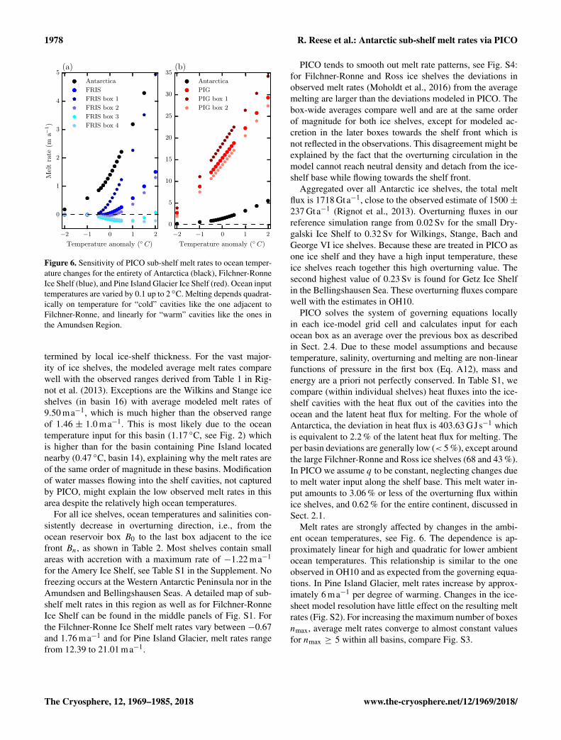
Figure 6. Sensitivity of PICO sub-shelf melt rates to ocean temper-ature changes for the entirety of Antarctica (black), Filchner-RonneIce Shelf (blue), and Pine Island Glacier Ice Shelf (red). Ocean inputtemperatures are varied by 0.1 up to 2 ◦C. Melting depends quadrat-ically on temperature for “cold” cavities like the one adjacent toFilchner-Ronne, and linearly for “warm” cavities like the ones inthe Amundsen Region.

termined by local ice-shelf thickness. For the vast major-ity of ice shelves, the modeled average melt rates comparewell with the observed ranges derived from Table 1 in Rig-not et al. (2013). Exceptions are the Wilkins and Stange iceshelves (in basin 16) with average modeled melt rates of9.50 ma−1, which is much higher than the observed rangeof 1.46 ± 1.0 ma−1. This is most likely due to the oceantemperature input for this basin (1.17 ◦C, see Fig. 2) whichis higher than for the basin containing Pine Island locatednearby (0.47 ◦C, basin 14), explaining why the melt rates areof the same order of magnitude in these basins. Modificationof water masses flowing into the shelf cavities, not capturedby PICO, might explain the low observed melt rates in thisarea despite the relatively high ocean temperatures.

For all ice shelves, ocean temperatures and salinities con-sistently decrease in overturning direction, i.e., from theocean reservoir box B0 to the last box adjacent to the icefront Bn, as shown in Table 2. Most shelves contain smallareas with accretion with a maximum rate of −1.22 ma−1

for the Amery Ice Shelf, see Table S1 in the Supplement. Nofreezing occurs at the Western Antarctic Peninsula nor in theAmundsen and Bellingshausen Seas. A detailed map of sub-shelf melt rates in this region as well as for Filchner-RonneIce Shelf can be found in the middle panels of Fig. S1. Forthe Filchner-Ronne Ice Shelf melt rates vary between −0.67and 1.76 ma−1 and for Pine Island Glacier, melt rates rangefrom 12.39 to 21.01 ma−1.

PICO tends to smooth out melt rate patterns, see Fig. S4:for Filchner-Ronne and Ross ice shelves the deviations inobserved melt rates (Moholdt et al., 2016) from the averagemelting are larger than the deviations modeled in PICO. Thebox-wide averages compare well and are at the same orderof magnitude for both ice shelves, except for modeled ac-cretion in the later boxes towards the shelf front which isnot reflected in the observations. This disagreement might beexplained by the fact that the overturning circulation in themodel cannot reach neutral density and detach from the ice-shelf base while flowing towards the shelf front.

Aggregated over all Antarctic ice shelves, the total meltflux is 1718 Gta−1, close to the observed estimate of 1500 ±237 Gta−1 (Rignot et al., 2013). Overturning fluxes in ourreference simulation range from 0.02 Sv for the small Dry-galski Ice Shelf to 0.32 Sv for Wilkings, Stange, Bach andGeorge VI ice shelves. Because these are treated in PICO asone ice shelf and they have a high input temperature, theseice shelves reach together this high overturning value. Thesecond highest value of 0.23 Sv is found for Getz Ice Shelfin the Bellingshausen Sea. These overturning fluxes comparewell with the estimates in OH10.

PICO solves the system of governing equations locallyin each ice-model grid cell and calculates input for eachocean box as an average over the previous box as describedin Sect. 2.4. Due to these model assumptions and becausetemperature, salinity, overturning and melting are non-linearfunctions of pressure in the first box (Eq. A12), mass andenergy are a priori not perfectly conserved. In Table S1, wecompare (within individual shelves) heat fluxes into the ice-shelf cavities with the heat flux out of the cavities into theocean and the latent heat flux for melting. For the whole ofAntarctica, the deviation in heat flux is 403.63 GJs−1 whichis equivalent to 2.2 % of the latent heat flux for melting. Theper basin deviations are generally low (< 5 %), except aroundthe large Filchner-Ronne and Ross ice shelves (68 and 43 %).In PICO we assume q to be constant, neglecting changes dueto melt water input along the shelf base. This melt water in-put amounts to 3.06 % or less of the overturning flux withinice shelves, and 0.62 % for the entire continent, discussed inSect. 2.1.

Melt rates are strongly affected by changes in the ambi-ent ocean temperatures, see Fig. 6. The dependence is ap-proximately linear for high and quadratic for lower ambientocean temperatures. This relationship is similar to the oneobserved in OH10 and as expected from the governing equa-tions. In Pine Island Glacier, melt rates increase by approx-imately 6 ma−1 per degree of warming. Changes in the ice-sheet model resolution have little effect on the resulting meltrates (Fig. S2). For increasing the maximum number of boxesnmax, average melt rates converge to almost constant valuesfor nmax ≥ 5 within all basins, compare Fig. S3.

The Cryosphere, 12, 1969–1985, 2018 www.the-cryosphere.net/12/1969/2018/

R. Reese et al.: Antarctic sub-shelf melt rates via PICO 1979

3.3 Transient evolution of PICO boxes and melt rates

PICO is capable of adjusting to changing ice-shelf geome-tries and migrating grounding lines. We demonstrate its be-havior as a module in PISM in a transient simulation. Basedon an Antarctic equilibrium state at 8 km resolution compa-rable to the state submitted to initMIP (Nowicki et al., 2016),we run PISM+PICO over time with a simple temperatureforcing applied: starting from equilibrium conditions, oceantemperatures increase linearly over 50 years until an ocean-wide warming of 1 ◦C is reached. It is then held constantover the next 250 modeled years. The Video S1 shows thetemporal evolution of the ocean temperature input for the iceshelf adjacent to Pine Island Glacier as well as the Filchner-Ronne Ice Shelf. The ocean temperature increase enhancesthe sub-shelf melting for both ice shelves, especially in thefirst box. Ice-shelf thinning reduces buttressing and causesthe grounding lines to retreat with the ocean boxes adjustingaccordingly.

4 Discussion

PICO models the dominant vertical overturning circulationin ice-shelf cavities and translates ocean conditions in frontof the ice shelves, either from observations or large-scaleocean models, into physically based sub-shelf melt rates.For present-day ocean fields and ice-shelf cavity geometries,PICO as an ocean module in PISM reproduces average meltrates of the same order of magnitude as observations for mostAntarctic ice shelves. With a single combination of over-turning parameter C and effective turbulent heat exchangeparameter γ ∗T applied to all shelves, a wide range of meltrates for the different ice shelves is obtained, reproducing thelarge-scale patterns observed in Antarctica. The results areconsistent across different ice-sheet and cavity model reso-lutions. Additionally, PICO reproduces the common patternof maximum melt close to the grounding line and decreas-ing melt rates towards the ice-shelf front, eventually with re-freezing in the shallow parts of the large ice shelves. The gov-erning model equations are solved for individual grid cells ofthe ice sheet model (and not for each ocean box with repre-sentative depth value), which allows spatial variability in theresulting melt rate field at comparatively smaller scale. PICOcan adapt to evolving cavities and is applicable to ice shelvesin two horizontal dimensions. It is hence suited as a sub-shelfmelt module for ice-sheet models.

Yet PICO is a coarse model designed as an ocean cou-pler for large-scale ice-sheet models. It is based on the OH10model and hence shares some simplifying assumptions withthat model: PICO does not resolve ocean dynamics and itparameterizes the vertical overturning circulation in the ice-shelf cavities which is given by one value for each ice shelf.The underlying box model equations of PICO do not resolvehorizontal ocean circulation in the ice-shelf cavities driven

by the Coriolis force nor seasonal melt variation due to in-trusion of warm water from the calving front during Australsummer. Hence, we do not expect that horizontal variationsor small scale patterns of basal melt are accurately capturedin PICO. Due to the box model formulation, maximum melt-ing in PICO is found directly at the grounding line and notslightly downstream as seen in the high-resolution coupledice–ocean simulation by, e.g., De Rydt and Gudmundsson(2016). We find that PICO tends to produce smoother meltrate patterns than observed, though the box-wide averagesare in good agreement with observations. The effect on icedynamics of small-scale differences in melt patterns in re-lation to the large-scale mean melt fluxes is not well estab-lished yet and needs further investigation. Following OH10,meltwater does not contribute to the volume flux in the cavityin PICO, introducing a minor error regarding mass conserva-tion. The relative error regarding mass conservation is how-ever small and below 0.7 % of the total overturning strengthin our reference run.

A necessary condition for the box model to work is fur-ther the assumption that melting outweighs accretion in boxB1 which is consistent with the majority of available obser-vations. In PICO, melt rates show a quadratic dependencyon ocean temperature input for lower temperatures, e.g., inthe Filchner-Ronne basin, and a rather linear dependency forhigher temperatures, e.g., in the Amundsen basin. This isconsistent with the results from OH10 and the implementedmelting physics assuming a constant coefficient for turbu-lent heat exchange. In contrast, P. R. Holland et al. (2008)employ a dependency of the turbulent heat exchange coef-ficient on the velocity of the overturning circulation, sug-gesting melt rates to respond quadratically to warming of theambient ocean water. Here we follow the approach taken inOH10.

Differently from the OH10 model and relying on muchlonger timescales of ice dynamics in comparison to oceandynamics, PICO assumes the overturning circulation to bein steady state. In their analysis, OH10 find unstable verti-cal water columns to occur only transiently, and hence forPICO a stable stratification of the vertical water column is as-sumed. Under these conditions, diffusive transport betweenthe boxes is generally small in OH10 and it is hence omit-ted in PICO. Because PICO also does not consider verticalvariations in ambient ocean density, under-ice flow is pre-vented from reaching neutral density and detaching from theice-shelf base on its way towards the shelf front. The spa-tial pattern of melting closer to the calving front of cold iceshelves may in such cases be not represented well.

PICO input is determined by averaging bottom tempera-tures and salinities over the continental shelf, this is donefor 19 different basins. Hence PICO – as a coarse model –misses the nuances of how ocean currents transport and mod-ify CDW over the regions being averaged. The procedure todetermine melt rates in PICO is based on the assumption thatocean water that is present on the continental shelf can ac-

www.the-cryosphere.net/12/1969/2018/ The Cryosphere, 12, 1969–1985, 2018

1980 R. Reese et al.: Antarctic sub-shelf melt rates via PICO

cess the ice-shelf cavities and reach their grounding lines.This implies for example, that barriers like sills that may pre-vent intrusion of warm CDW are not accounted for and mightexplain why PICO melting is too high for the ice shelves lo-cated along the Southern Antarctic Peninsula. Such phenom-ena could be tested by varying the ocean input of PICO byevolving the temperature and salinity outside of the cavityover time. Because of the dependence of sub-shelf meltingon the local pressure of the ice column above, the model isnot fully energy conserving. For the estimated heat fluxes, therelative error is lower than 2.2 % of the latent heat flux due tosub-shelf melting. Hence, we consider our choice of modelsimplifications as justified, as it introduces small errors in theheat and mass balances in our reference simulation.

PICO is computationally fast, as it uses analytic solutionsof the equations of motion with a small number of boxesalong the ice shelf. As boundary conditions for PICO areaggregated based on predefined regional basins, the modelcan act as an efficient coupler of large-scale ice-sheet andocean models. For this purpose, heat flux into the ice shouldbe added to the boundary layer melt formulation.

5 Conclusions

The Antarctic Ice Sheet plays a vital role in modulatingglobal sea level. The ice grounded below sea level in its ma-rine basins is susceptible to ocean forcing and might respondnonlinearly to changes in ocean boundary conditions (Mer-cer, 1978; Schoof, 2007). We therefore need carefully esti-mated conditions at the ice–ocean boundary to better con-strain the dynamics of the Antarctic ice and its contributionto sea-level rise for the past and the future.

The PICO model presented here provides a physics-basedyet efficient approach for estimating the ocean circulation be-low ice shelves and the heat provided for ice-shelf melt. Themodel extends the one-horizontal dimensional ocean boxmodel by OH10 to realistic ice-shelf geometries followingthe shape of the grounding line and calving front. PICO is acomparably simple alternative to full ocean models, but goesbeyond local melt parameterizations, which do not accountfor the circulation below ice shelves. We find a set of possi-ble parameters for present-day ocean conditions and ice ge-ometries which yield PICO melt rates in agreement with av-erage melt rate observations. PICO qualitatively reproducesthe general pattern of ice-shelf melt, with high melting atthe grounding line and low melting or refreezing towardsthe calving front. Its sensitivity to changes in input oceantemperatures and model parameters is comparable to earlierestimates (Holland and Jenkins, 1999; Olbers and Hellmer,2010). The model accurately captures the large variety of ob-served Antarctic melt rates using only two calibrated param-eters applied to all ice shelves.

The ocean models that are part of the large Earth systemand global circulation models do not yet resolve the circula-tion below ice shelves. PICO is able to fill this gap and canbe used as an intermediary between global circulation mod-els and ice sheet models. We expect that PICO will be usefulfor providing ocean forcing to ice sheet models with the stan-dardized input from climate model intercomparison projectslike CMIP5 and CMIP6 (Taylor et al., 2012; Meehl et al.,2014; Eyring et al., 2016). Since PICO can deal with evolv-ing ice-shelf geometries in a computationally efficient way, itis in particular suitable for modeling the ice sheet evolutionon paleo-climate timescales as well as for future projections.

PICO is implemented as a module in the open-source Par-allel Ice Sheet Model (PISM). The source code is fully ac-cessible and documented as we want to encourage improve-ments and implementation in other ice sheet models. Thisincludes the adaption to other ice sheets than present-dayAntarctica.

Code availability. The PICO code used for this publication is avail-able under Reese et al. (2018). For further use of PICO please referto the latest version at https://github.com/pism/pism/commits/dev.

Data availability. The data that support the findings of this studyare available from the corresponding authors upon request.

The Cryosphere, 12, 1969–1985, 2018 www.the-cryosphere.net/12/1969/2018/

R. Reese et al.: Antarctic sub-shelf melt rates via PICO 1981

Appendix A: Derivation of the analytic solutions

Here, we derive the analytic solutions of the equations sys-tem describing the overturning circulation (see Sect. 2.1) andthe melting at the ice–ocean interface (see Sect. 2.2).

For box Bk with k > 1 we solve progressively for melt ratemk , temperature Tk and salinity Sk in box Bk , dependent onthe local pressure pk , the area of box adjacent to the ice-shelf base Ak and the temperature Tk−1 and salinity Sk−1 ofthe upstream box Bk−1. For box B1, we additionally solvefor the overturning q as explained below. These derivationsadvance the ideas presented in the appendix of OH10. As-suming steady state conditions, the balance Eqs. (1) and (2)for box Bk from Sect. 2.1 are

0= q (Tk−1− Tk)+AkγT (Tbk − Tk)+Akmk (Tbk − Tk),

0= q (Sk−1− Sk)+AkγS (Sbk − Sk)+Akmk (Sbk − Sk) . (A1)

The heat fluxes balance at the boundary layer interface, i.e.,the heat flux across the boundary layer due to turbulent mix-ingQT = ρwcpγT (Tbk − Tk) equals the heat flux due to melt-ing or freezing QTb =−ρiLmk , omitting the heat flux intothe ice. This yields

γT (Tbk − Tk)=−νλmk, (A2)

where ν = ρi/ρw ∼ 0.89, λ= L/cp ∼ 84 ◦C. Regarding thesalt flux balance in the boundary layer, with QS =

ρwγS (Sbk − Sk) at the lower interface of the boundarylayer and “virtual” salt flux due to meltwater input QSb =

−ρiSbkmk , we obtain

γS (Sbk − Sk)=−νSbkmk. (A3)

Inserting Eqs. (A2) and (A3) into Eqs. (A1) yields

0= q (Tk−1− Tk)−Akmkνλ+Akmk (Tbk − Tk) ,

0= q (Sk−1− Sk)−AkmkνSbk +Akmk (Sbk − Sk) .

Comparing (Tbk − Tk)� νλ≈ 75 ◦C, allows us to neglectthe last term in the temperature equation. Considering thelast two terms of the salinity equation, we find that Sk >(1− ν)Sbk ≈ 0.1Sbk , allowing us to neglect the terms con-taining Sbk , which simplifies the equations to

0= q (Tk−1− Tk)−Akνλmk

0= q (Sk−1− Sk)−AkmkSk. (A4)

We use a simplified version of the melt law described byMcPhee (1992) and detailed in Sect. 2.2, which makes useof Eqs. (6) and (5) in which the salinity in the boundary layerSbk is replaced by salinity of the ambient ocean water:

mk =−γ ∗Tνλ(aSk + b− cpk − Tk) . (A5)

Holland and Jenkins (1999) suggest that this simplificationrequires γ ∗T to be a factor of 1.35 to 1.6 smaller than γT

in the 3-equation formulation for the constant values of γTranging from 3×10−5 to 5×10−5 ms−1 used in OH10. Thisimplies that γ ∗T ranges from 2.2× 10−5 to 3.2× 10−5 ms−1,which is consistent with the parameter range we derive inSect. 3.1. We apply this assumption in the computation ofmelt rates. For the solution of the transport Eqs. (A1), it isessential to take the salinity of the boundary layer Sbk into ac-count, since otherwise the salinity transport equation wouldreduce to Sk = Sk−1 and the overturning circulation, whichis predominantly haline driven, would be reduced. Insertingthe simplified melt law in Eq. (A4) yields

0= q (Tk−1− Tk)+Akγ ∗Tνλ(aSk + b− cpk − Tk) νλ,

0= q (Sk−1− Sk)+Akγ ∗Tνλ(aSk + b− cpk − Tk) Sk.

Replacing x = Tk−1−Tk , y = Sk−1−Sk , T ∗ = aSk−1+b−

cpk − Tk−1, g1 = Akγ∗T and g2 =

g1νλ

, we obtain

0= qx+ g1(T ∗+ x− ay

), (A6)

0= qy+ g2 (Sk−1− y)(T ∗+ x− ay

). (A7)

We simplify the previous equations as follows. RewritingEq. (A6) as

(T ∗+ x− ay

)=−qx

g1

and inserting it into Eq. (A7), we obtain

0= qy+ g2(Sk−1− y)

(−qx

g1

)= qy− qx

Sk−1− y

νλ

⇐⇒ 0= νλy− Sk−1x+ xy

⇐⇒ 0= (νλ+ x)y− Sk−1x

⇒ y =Sk−1x

νλ+ x.

Note that we can divide the first line by q since, by the modelassumptions, q > 0. Because x = Tk−1− Tk � νλ≈ 75 ◦C,we may approximate

y ≈Sk−1x

νλ. (A8)

Using this approximation, we may proceed to solve the sys-tem of equations. Since we also need to solve for the over-turning q in boxB1, which is adjacent to the grounding line, aslightly different approach is needed than for the other boxes,as discussed in the next section.

A1 Solution for box B1

The overturning flux q is parameterized as

q = Cρ∗ ( β (S0− S1)−α (T0− T1) ) , (A9)

www.the-cryosphere.net/12/1969/2018/ The Cryosphere, 12, 1969–1985, 2018

1982 R. Reese et al.: Antarctic sub-shelf melt rates via PICO

in the model, see Sect. 2.1. Substituting this equation intoEqs. (A6) and (A7), we obtain

0= αx2−βxy−

g1

Cρ∗

(T ∗+ x− ay

), (A10)

0=−βy2+αxy−

g2

Cρ∗(S0− y)

(T ∗+ x− ay

). (A11)

Inserting the approximation for y from Eq. (A8) into theEq. (A10), we obtain a quadratic equation for x,

(βs−α)x2+

g1

Cρ∗

(T ∗+ x (1− as)

)= 0,

with s = S0/νλ. Since as =−0.057× S0/74.76=−0.000762× S0� 1, we can omit the last part of thelast term,

(βs−α)x2+

g1

Cρ∗

(T ∗+ x

)= 0.

Rearranging (assuming that βs−α > 0, which we demon-strate below), we obtain

x2+

g1

Cρ∗ (βs−α)x+

g1T∗

Cρ∗ (βs−α)= 0,

and hence we obtain the solution

x =−g1

2Cρ∗ (βs−α)

±

√(g1

2Cρ∗ (βs−α)

)2

−g1T

∗

Cρ∗ (βs−α). (A12)

The temperature in the box B1 near the grounding lineis supposed to be smaller than in the ocean box B0,since, in general, melting will occur in box B1 and henceT1 < T0, or equivalently x = T0− T1 > 0. Furthermore, weknow that g1/(Cρ∗)= A1γ

∗T /(Cρ∗) is positive, as all fac-

tors are positive. Since α = 7.5× 10−5, β = 7.7× 10−4 ands = S0/(νλ)= S0/74.76≥ 0.4, it follows that βs > α. Thismeans that the first summand of Eq. (A12) is negative andthe second (negative) solution can be excluded. From here,we use T1 = T0+ x and y = xS0/(νλ) to solve for T1, S1,m1 and q.

A2 Solution for box Bk , k > 1

Now, we give the solution for the other boxes Bk with k >1. By inserting the approximation for y in Eq. (A8) intoEq. (A6), we can solve for x as

0= qx+ g1

(T ∗+ x− a

Sk−1x

νλ

)⇐⇒0= qx+ g1T

∗+ g1x− g2 a Sk−1 x

⇐⇒− g1T∗= x (q + g1− g2 Sk−1 a)

⇐⇒x =−g1T

∗

q + g1− g2 a Sk−1. (A13)

The denominator is positive, as all terms are positive, and thesign of the numerator depends on T ∗. The equation can nowbe solved for Tk , and then Eq. (A8) for Sk and Eq. (13) formk .

Appendix B: Motivation for geometric rule

Here, we want to motivate the rule that determines the extentof the boxes under each ice shelf. The rule aims at equal areasfor all boxes. Assuming a half-circle with radius r = 1, wewant to split it into a fixed number n of equal-area rings. Gen-eralized to the individual shapes of ice shelves, we will de-fine the “radius” of an ice shelf as r = 1− dGL/(dGL+ dIF).We define r1 = 1 the outer (grounding-line ward) radius ofthe half-circle ring covering an area A1 and correspondingto box B1 adjacent to the grounding line, r2 as the outerradius of second outer-most half-ring, etc. The box Bk isthen given by all shelf cells with horizontal coordinates (x,y) such that rk+1 ≤ r (x,y)≤ rk where rn+1 = 0 is the cen-ter point of the circle. We can use these to determine theareas An = 0.5πr2

n, An−1 = 0.5π(r2n−1− r

2n

), . . ., An−k =

0.5π(r2n−k − r

2n−k+1

). If we require that A1 = A2 = . . .=

An, then, solving progressively, rn−k =√k+ 1 rn. By our

assumption is r1 = 1, hence 1= rn−(n−1) =√nrn. This im-

plies that rn = 1/√n and thus rn−k =

√k+1n

. Hence, the

box Bk for k = 1, . . .,n is defined as 1−√(n− k+ 1)/n≤

dGL/(dGL+ dIF)≤ 1−√(n− k)/n.

The Cryosphere, 12, 1969–1985, 2018 www.the-cryosphere.net/12/1969/2018/

R. Reese et al.: Antarctic sub-shelf melt rates via PICO 1983

The Supplement related to this article is available onlineat https://doi.org/10.5194/tc-12-1969-2018-supplement.

Author contributions. All authors designed the model. RW con-ceived the study. RR, RW, TA, and MM implemented PICO as amodule in PISM. RR conducted the model experiments. MM cre-ated the Antarctic equilibrium simulation for the Video S1 in theSupplement. RR prepared the manuscript with contributions fromall co-authors.

Competing interests. The authors declare that they have no conflictof interest.

Acknowledgements. Development of PISM is supported by NASAgrant NNX17AG65G and NSF grants PLR-1603799 and PLR-1644277. Torsten Albrecht was supported by DFG priority programSPP 1158, project numbers LE1448/6-1 and LE1448/7-1. MatthiasMengel was supported by the AXA Research Fund. Ronja Reesewas supported by the German Academic National Foundation, thepostgraduate scholarship programme of the state of Brandenburgand the Evangelisches Studienwerk Villigst. The project is furthersupported by the German Climate Modeling Initiative (PalMod) andthe Leibniz project DominoES. Xylar Asay-Davis was supported bythe US Department of Energy, Office of Science, Office of Biolog-ical and Environmental Research under award no. DE-SC0013038.The authors gratefully acknowledge the European Regional Devel-opment Fund (ERDF), the German Federal Ministry of Educationand Research and the Land Brandenburg for supporting this projectby providing resources on the high performance computer systemat the Potsdam Institute for Climate Impact Research.

We thank Frank Pattyn and the anonymous reviewer fortheir helpful comments on the manuscript. We are grateful toConstantine Khroulev for his excellent support in improving theimplementation of PICO in PISM. We are very thankful to HartmutH. Hellmer and Dirk Olbers for their helpful comments and theirongoing support in further developing their original ocean boxmodel.

Edited by: Eric LarourReviewed by: Frank Pattyn and one anonymous referee

References

Asay-Davis, X. S., Cornford, S. L., Durand, G., Galton-Fenzi, B.K., Gladstone, R. M., Gudmundsson, G. H., Hattermann, T., Hol-land, D. M., Holland, D., Holland, P. R., Martin, D. F., Mathiot,P., Pattyn, F., and Seroussi, H.: Experimental design for threeinterrelated marine ice sheet and ocean model intercomparisonprojects: MISMIP v. 3 (MISMIP +), ISOMIP v. 2 (ISOMIP +)and MISOMIP v. 1 (MISOMIP1), Geosci. Model Dev., 9, 2471–2497, https://doi.org/10.5194/gmd-9-2471-2016, 2016.

Beckmann, A. and Goosse, H.: A parameterization of ice shelf-ocean interaction for climate models, Ocean Model., 5, 157–170,https://doi.org/10.1016/S1463-5003(02)00019-7, 2003.

Beckmann, J., Perrette, M., and Ganopolski, A.: Simple models forthe simulation of submarine melt for a Greenland glacial systemmodel, The Cryosphere, 12, 301–323, https://doi.org/10.5194/tc-12-301-2018, 2018.

Bueler, E. and Brown, J.: Shallow shelf approximation as a “slidinglaw” in a thermomechanically coupled ice sheet model, J. Geo-phys. Res., 114, F03008, https://doi.org/10.1029/2008JF001179,2009.

Carroll, D., Sutherland, D. A., Shroyer, E. L., Nash, J. D.,Catania, G. A., and Stearns, L. A.: Modeling TurbulentSubglacial Meltwater Plumes: Implications for Fjord-ScaleBuoyancy-Driven Circulation, J. Phys. Oceanogr., 45, 2169–2185, https://doi.org/10.1175/JPO-D-15-0033.1, 2015.

Depoorter, M. A., Bamber, J. L., Griggs, J. A., Lenaerts, J. T. M.,Ligtenberg, S. R. M., van den Broeke, M. R., and Moholdt, G.:Calving fluxes and basal melt rates of Antarctic ice shelves., Na-ture, 502, 89–92, https://doi.org/10.1038/nature12567, 2013.

De Rydt, J. and Gudmundsson, G. H.: Coupled ice shelf-ocean modeling and complex grounding line retreat froma seabed ridge, J. Geophys. Res.-Earth, 121, 865–880,https://doi.org/10.1002/2015JF003791, 2016.

Dupont, T. K. and Alley, R. B.: Assessment of the importance ofice-shelf buttressing to ice-sheet flow, Geophys. Res. Lett., 32,L04503, https://doi.org/10.1029/2004GL022024, 2005.

Eyring, V., Bony, S., Meehl, G. A., Senior, C. A., Stevens, B.,Stouffer, R. J., and Taylor, K. E.: Overview of the CoupledModel Intercomparison Project Phase 6 (CMIP6) experimen-tal design and organization, Geosci. Model Dev., 9, 1937–1958,https://doi.org/10.5194/gmd-9-1937-2016, 2016.

Favier, L., Durand, G., Cornford, S. L., Gudmundsson, G. H.,Gagliardini, O., Gillet-Chaulet, F., Zwinger, T., Payne, A. J.,and Le Brocq, A. M.: Retreat of Pine Island Glacier controlledby marine ice-sheet instability, Nat. Clim. Change, 5, 117–121,https://doi.org/10.1038/nclimate2094, 2014.

Feldmann, J., Albrecht, T., Khroulev, C., Pattyn, F., and Levermann,A.: Resolution-dependent performance of grounding line motionin a shallow model compared with a full-Stokes model accord-ing to the MISMIP3d intercomparison, J. Glaciol., 60, 353–360,https://doi.org/10.3189/2014JoG13J093, 2014.

Fretwell, P., Pritchard, H. D., Vaughan, D. G., Bamber, J. L., Bar-rand, N. E., Bell, R., Bianchi, C., Bingham, R. G., Blanken-ship, D. D., Casassa, G., Catania, G., Callens, D., Conway, H.,Cook, A. J., Corr, H. F. J., Damaske, D., Damm, V., Ferracci-oli, F., Forsberg, R., Fujita, S., Gim, Y., Gogineni, P., Griggs,J. A., Hindmarsh, R. C. A., Holmlund, P., Holt, J. W., Jacobel,R. W., Jenkins, A., Jokat, W., Jordan, T., King, E. C., Kohler,J., Krabill, W., Riger-Kusk, M., Langley, K. A., Leitchenkov,G., Leuschen, C., Luyendyk, B. P., Matsuoka, K., Mouginot,J., Nitsche, F. O., Nogi, Y., Nost, O. A., Popov, S. V., Rignot,E., Rippin, D. M., Rivera, A., Roberts, J., Ross, N., Siegert,M. J., Smith, A. M., Steinhage, D., Studinger, M., Sun, B.,Tinto, B. K., Welch, B. C., Wilson, D., Young, D. A., Xiangbin,C., and Zirizzotti, A.: Bedmap2: improved ice bed, surface andthickness datasets for Antarctica, The Cryosphere, 7, 375–393,https://doi.org/10.5194/tc-7-375-2013, 2013.

www.the-cryosphere.net/12/1969/2018/ The Cryosphere, 12, 1969–1985, 2018

1984 R. Reese et al.: Antarctic sub-shelf melt rates via PICO

Goldberg, D. N., Little, C. M., Sergienko, O. V., Gnanadesikan,A., Hallberg, R., and Oppenheimer, M.: Investigation of landice–ocean interaction with a fully coupled ice-ocean model:1. Model description and behavior, J. Geophys. Res., 117,F02037, https://doi.org/10.1029/2011JF002246, 2012.

Greenbaum, J. S., Blankenship, D. D., Young, D. A., Richter, T. G.,Roberts, J. L., Aitken, A. R. A., Legresy, B., Schroeder, D. M.,Warner, R. C., van Ommen, T. D., and Siegert, M. J.: Ocean ac-cess to a cavity beneath Totten Glacier in East Antarctica, Nat.Geosci., 8, 294–298,https://doi.org/10.1038/NGEO2388, 2015.

Gudmundsson, G. H., Krug, J., Durand, G., Favier, L., and Gagliar-dini, O.: The stability of grounding lines on retrograde slopes,The Cryosphere, 6, 1497–1505, https://doi.org/10.5194/tc-6-1497-2012, 2012.

Hellmer, H. and Olbers, D.: A two-dimensional model for the ther-mohaline circulation under an ice shelf, Antarct. Sci., 1, 325–336, https://doi.org/10.1017/S0954102089000490, 1989.

Hellmer, H. H., Kauker, F., Timmermann, R., and Hatter-mann, T.: The fate of the southern Weddell Sea continen-tal shelf in a warming climate, J. Climate, 30, 4337–4350,https://doi.org/10.1175/JCLI-D-16-0420.1, 2017.

Holland, D. M. and Jenkins, A.: Modeling ThermodynamicIce–Ocean Interactions at the Base of an Ice Shelf, J. Phys.Oceanogr., 29, 1787–1800, https://doi.org/10.1175/1520-0485(1999)029<1787:MTIOIA>2.0.CO;2, 1999.

Holland, D. M., Thomas, R. H., de Young, B., Ribergaard, M. H.,and Lyberth, B.: Acceleration of Jakobshavn Isbrætriggeredby warm subsurface ocean waters, Nat. Geosci., 1, 659–664,https://doi.org/10.1038/ngeo316, 2008.

Holland, P. R., Feltham, D. L., and Jenkins, A.: IceShelf Water plume flow beneath Filchner-Ronne IceShelf, Antarctica, J. Geophys. Res., 112, C05044,https://doi.org/10.1029/2006JC003915, 2007.

Holland, P. R., Jenkins, A., and Holland, D. M.: The Response of IceShelf Basal Melting to Variations in Ocean Temperature, J. Cli-mate, 21, 2558–2572, https://doi.org/10.1175/2007JCLI1909.1,2008.

Hutter, K.: Theoretical glaciology: material science of ice and themechanics of glaciers and ice sheets, Springer, vol. 1, 1983.

Jacobs, S. S., Hellmer, H., Doake, C. S. M., Jenkins, A.,and Frolich, R. M.: Melting of ice shelves and themass balance of Antarctica, J. Glaciol., 38, 375–387,https://doi.org/10.3189/S0022143000002252, 1992.

Jacobs, S. S., Jenkins, A., Giulivi, C. F., and Dutrieux,P.: Stronger ocean circulation and increased melting underPine Island Glacier ice shelf, Nat. Geosci., 4, 519–523,https://doi.org/10.1038/ngeo1188, 2011.

Jenkins, A.: A one-dimensional model of ice shelf-ocean interaction, J. Geophys. Res., 96, 20671–20677,https://doi.org/10.1029/91JC01842, 1991.

Jenkins, A.: Convection-Driven Melting near the Grounding Linesof Ice Shelves and Tidewater Glaciers, J. Phys. Oceanogr., 41,2279–2294, https://doi.org/10.1175/JPO-D-11-03.1, 2011.

Jenkins, A., Hellmer, H. H., and Holland, D. M.: TheRole of Meltwater Advection in the Formulation of Con-servative Boundary Conditions at an Ice-Ocean Interface,J. Phys. Oceanogr., 31, 285–296, https://doi.org/10.1175/1520-0485(2001)031<0285:TROMAI>2.0.CO;2, 2001.

Joughin, I., Alley, R. B., and Holland, D. M.: Ice-SheetResponse to Oceanic Forcing, Science, 338, 1172–1176,https://doi.org/10.1126/science.1226481, 2012.

Joughin, I., Smith, B. E., and Medley, B.: Marine IceSheet Collapse Potentially Under Way for the ThwaitesGlacier Basin, West Antarctica, Science, 344, 735–738,https://doi.org/10.1126/science.1249055, 2014.

Lazeroms, W. M. J., Jenkins, A., Gudmundsson, G. H., and van deWal, R. S. W.: Modelling present-day basal melt rates for Antarc-tic ice shelves using a parametrization of buoyant meltwaterplumes, The Cryosphere, 12, 49–70, https://doi.org/10.5194/tc-12-49-2018, 2018.

Lewis, E. L. and Perkin, R. G.: Ice pumps andtheir rates, J. Geophys. Res., 91, 11756–11762,https://doi.org/10.1029/JC091iC10p11756, 1986.

Little, C. M., Goldberg, D., Gnanadesikan, A., andOppenheimer, M.: On the coupled response toice-shelf basal melting, J. Glaciol., 58, 203–215,https://doi.org/10.3189/2012JoG11J037, 2012.

Liu, Y., Moore, J. C., Cheng, X., Gladstone, R. M., Bassis,J. N., Liu, H., Wen, J., and Hui, F.: Ocean-driven thin-ning enhances iceberg calving and retreat of Antarcticice shelves, P. Natl. Acad. Sci. USA, 112, 3263–3268,https://doi.org/10.1073/pnas.1415137112, 2015.

MacGregor, J. A., Catania, G. A., Markowski, M. S., andAndrews, A. G.: Widespread rifting and retreat of ice-shelf margins in the eastern Amundsen Sea Embay-ment between 1972 and 2011, J. Glaciol., 58, 458–466,https://doi.org/10.3189/2012JoG11J262, 2012.

Martin, M. A., Winkelmann, R., Haseloff, M., Albrecht, T., Bueler,E., Khroulev, C., and Levermann, A.: The Potsdam Parallel IceSheet Model (PISM-PIK) – Part 2: Dynamic equilibrium simu-lation of the Antarctic ice sheet, The Cryosphere, 5, 727–740,https://doi.org/10.5194/tc-5-727-2011, 2011.

McDougall, T. J. and Barker, P. M.: Getting started with TEOS-10and the Gibbs Seawater (GSW) Oceanographic Toolbox, May,SCOR/IAPSO WG1207, available at: http://www.teos-10.org/pubs/Getting_Started.pdf (last access: 15 May 2018), 2011.

McPhee, M. G.: Turbulent heat flux in the upper oceanunder sea ice, J. Geophys. Res., 97, 5365–5379,https://doi.org/10.1029/92JC00239, 1992.

McPhee, M. G.: Parameterization of mixing in the ocean boundarylayer, J. Marine Syst., 21, 55–65, https://doi.org/10.1016/S0924-7963(99)00005-6, 1999.

Meehl, G. A., Moss, R., Taylor, K. E., Eyring, V., Stouffer, R. J.,Bony, S., and Stevens, B.: Climate Model Intercomparisons:Preparing for the Next Phase, Eos T. Am. Geophys. Un., 95, 77–78, https://doi.org/10.1002/2014EO090001, 2014.

Mercer, J. H.: West Antarctic ice sheet and CO2 greenhouse effect– A threat of disaster, Nature, 271, 321–325, 1978.

Moholdt, G., Padman, L., and Fricker, H. A.: Basal mass budget ofRoss and Filchner-Ronne ice shelves, Antarctica, derived fromLagrangian analysis of ICESat altimetry, J. Geophys. Res.-Earth,119, 2361–2380, https://doi.org/10.1002/2014JF003171, 2014.

Moholdt, G., Padman, L., and Fricker, H. A.: Elevationchange and mass budget of Ross and Filchner-Ronne iceshelves, Antarctica, Norwegian Polar Institute, Tromsø, Nor-way, https://doi.org/10.21334/npolar.2016.cae21585 (last ac-cess:n 12 June 2018), 2016.

The Cryosphere, 12, 1969–1985, 2018 www.the-cryosphere.net/12/1969/2018/

R. Reese et al.: Antarctic sub-shelf melt rates via PICO 1985

Morland, L. W.: Unconfined Ice-Shelf Flow, Springer Nether-lands, Dordrecht, 99–116, https://doi.org/10.1007/978-94-009-3745-1_6, 1987.

Mouginot, J., Rignot, E., and Scheuchl, B.: Sustained increase inice discharge from the Amundsen Sea Embayment, West Antarc-tica, from 1973 to 2013, Geophys. Res. Lett., 41, 1576–1584,https://doi.org/10.1002/2013GL059069, 2014.

Nowicki, S. M. J., Payne, A., Larour, E., Seroussi, H., Goelzer,H., Lipscomb, W., Gregory, J., Abe–Ouchi, A., and Shep-herd, A.: Ice Sheet Model Intercomparison Project (ISMIP6)contribution to CMIP6, Geosci. Model Dev., 9, 4521–4545,https://doi.org/10.5194/gmd-9-4521-2016, 2016.

Olbers, D. and Hellmer, H.: A box model of circulation andmelting in ice shelf caverns, Ocean Dynam., 60, 141–153,https://doi.org/10.1007/s10236-009-0252-z, 2010.

Paolo, F. S., Fricker, H. A., and Padman, L.: Volume loss fromAntarctic ice shelves is accelerating, Science, 348, 327–332,https://doi.org/10.1126/science.aaa0940, 2015.

Pattyn, F., Perichon, L., Durand, G., Favier, L., Gagliardini,O., Hindmarsh, R. C., Zwinger, T., Albrecht, T., Cornford,S., Docquier, D., Fürst, J. J., Goldberg, D., Gudmunds-son, G. H., Humbert, A., Hütten, M., Huybrechts, P., Jou-vet, G., Kleiner, T., Larour, E., Martin, D., Morlighem, M.,Payne, A. J., Pollard, D., Rückamp, M., Rybak, O., Seroussi,H., Thoma, M., and Wilkens, N.: Grounding-line migra-tion in plan-view marine ice-sheet models: results of theice2sea MISMIP3d intercomparison, J. Glaciol., 59, 410–422,https://doi.org/10.3189/2013JoG12J129, 2013.

Payne, A. J., Holland, P. R., Shepherd, A. P., Rutt, I. C., Jenkins, A.,and Joughin, I.: Numerical modeling of ocean-ice interactionsunder Pine Island Bay’s ice shelf, J. Geophys. Res.-Oceans, 112,C10019, https://doi.org/10.1029/2006JC003733, 2007.

Pollard, D. and DeConto, R. M.: Description of a hybrid ice sheet-shelf model, and application to Antarctica, Geosci. Model Dev.,5, 1273–1295, https://doi.org/10.5194/gmd-5-1273-2012, 2012.

Pritchard, H. D., Ligtenberg, S. R. M., Fricker, H. A., Vaughan,D. G., van den Broeke, M. R., and Padman, L.: Antarctic ice-sheet loss driven by basal melting of ice shelves, Nature, 484,502–505, https://doi.org/10.1038/nature10968, 2012.

Reese, R., Albrecht, T., Mengel, M., Winkelmann, R., andother PISM authors: pism/pik/pico_dev: PISM+PICO versionas used in Reese et al., The Cryosphere publication, Zenodo,https://doi.org/10.5281/zenodo.1248799, last access: 18 May2018.

Rignot, E., Jacobs, S., Mouginot, J., and Scheuchl, B.: Ice-shelf melting around Antarctica, Science, 341, 266–270,https://doi.org/10.1126/science.1235798, 2013.

Schmidtko, S., Heywood, K. J., Thompson, A. F., and Aoki, S.:Multidecadal warming of Antarctic waters, Science, 346, 1227–1231, https://doi.org/10.1126/science.1256117, 2014.

Schoof, C.: Marine ice-sheet dynamics. Part 1. The case of rapidsliding, J. Fluid Mech., 573, 27–55, 2007.

Seroussi, H., Nakayama, Y., Larour, E., Menemenlis, D.,Morlighem, M., Rignot, E., and Khazendar, A.: Continued retreatof Thwaites Glacier, West Antarctica, controlled by bed topogra-phy and ocean circulation, Geophys. Res. Lett., 44, 6191–6199,https://doi.org/10.1002/2017GL072910, 2017.

Taylor, K. E., Stouffer, R. J., and Meehl, G. A.: An Overview ofCMIP5 and the Experiment Design, B. Am. Meteorol. Soc., 93,485–498, https://doi.org/10.1175/BAMS-D-11-00094.1, 2012.

Thoma, M., Jenkins, A., Holland, D., and Jacobs, S.: ModellingCircumpolar Deep Water intrusions on the Amundsen Sea con-tinental shelf, Antarctica, Geophys. Res. Lett., 35, L18602,https://doi.org/10.1029/2008GL034939, 2008.

Thoma, M., Determann, J., Grosfeld, K., Goeller, S., andHellmer, H. H.: Future sea-level rise due to projected oceanwarming beneath the Filchner Ronne Ice Shelf: A cou-pled model study, Earth Planet. Sc. Lett., 431, 217–224,https://doi.org/10.1016/j.epsl.2015.09.013, 2015.

Thomas, R. H.: Ice Shelves: a Review, J. Glaciol., 24, 273–286,https://doi.org/10.3189/S0022143000014799, 1979.

Winkelmann, R., Martin, M. A., Haseloff, M., Albrecht, T., Bueler,E., Khroulev, C., and Levermann, A.: The Potsdam ParallelIce Sheet Model (PISM-PIK) – Part 1: Model description, TheCryosphere, 5, 715–726, https://doi.org/10.5194/tc-5-715-2011,2011.

Wouters, B., Martin-Espanol, A., Helm, V., Flament, T., vanWessem, J. M., Ligtenberg, S. R., van den Broeke, M. R., andBamber, J. L.: Glacier mass loss. Dynamic thinning of glacierson the Southern Antarctic Peninsula, Science, 348, 899–903,https://doi.org/10.1126/science.aaa5727, 2015.

Zwally, H. J., Giovinetto, M. B., Beckley, M. A., and Saba,J. L.: Antarctic and Greenland Drainage Systems, GSFCCryospheric Sciences Laboratory, at available at: https://icesat4.gsfc.nasa.gov/cryo_data/ant_grn_drainage_systems.php (last ac-cess: 15 May 2018), 2012.

www.the-cryosphere.net/12/1969/2018/ The Cryosphere, 12, 1969–1985, 2018