antenna diversity with opportunistic combining

Department of Science and Technology Institutionen för teknik och naturvetenskap Linköping University Linköpings universitet

gnipökrroN 47 106 nedewS ,gnipökrroN 47 106-ES

LiU-ITN-TEK-A--12/083--SE

Antenna diversity withopportunistic combining

Md. Khalilur Rahman

Chuanhui Xia

2012-12-14

LiU-ITN-TEK-A--12/083--SE

Antenna diversity withopportunistic combining

Examensarbete utfört i Elekroteknikvid Tekniska högskolan vid

Linköpings universitet

Md. Khalilur RahmanChuanhui Xia

Handledare Magnus KarlssonExaminator Shaofang Gong

Norrköping 2012-12-14

Upphovsrätt

Detta dokument hålls tillgängligt på Internet – eller dess framtida ersättare –under en längre tid från publiceringsdatum under förutsättning att inga extra-ordinära omständigheter uppstår.

Tillgång till dokumentet innebär tillstånd för var och en att läsa, ladda ner,skriva ut enstaka kopior för enskilt bruk och att använda det oförändrat förickekommersiell forskning och för undervisning. Överföring av upphovsrättenvid en senare tidpunkt kan inte upphäva detta tillstånd. All annan användning avdokumentet kräver upphovsmannens medgivande. För att garantera äktheten,säkerheten och tillgängligheten finns det lösningar av teknisk och administrativart.

Upphovsmannens ideella rätt innefattar rätt att bli nämnd som upphovsman iden omfattning som god sed kräver vid användning av dokumentet på ovanbeskrivna sätt samt skydd mot att dokumentet ändras eller presenteras i sådanform eller i sådant sammanhang som är kränkande för upphovsmannens litteräraeller konstnärliga anseende eller egenart.

För ytterligare information om Linköping University Electronic Press seförlagets hemsida http://www.ep.liu.se/

Copyright

The publishers will keep this document online on the Internet - or its possiblereplacement - for a considerable time from the date of publication barringexceptional circumstances.

The online availability of the document implies a permanent permission foranyone to read, to download, to print out single copies for your own use and touse it unchanged for any non-commercial research and educational purpose.Subsequent transfers of copyright cannot revoke this permission. All other usesof the document are conditional on the consent of the copyright owner. Thepublisher has taken technical and administrative measures to assure authenticity,security and accessibility.

According to intellectual property law the author has the right to bementioned when his/her work is accessed as described above and to be protectedagainst infringement.

For additional information about the Linköping University Electronic Pressand its procedures for publication and for assurance of document integrity,please refer to its WWW home page: http://www.ep.liu.se/

© Md. Khalilur Rahman, Chuanhui Xia

Antenna Diversity with

Opportunistic combining

Institute of Technology

(2012)

Authors: Supervisor and examiner:

Md. Khalilur Rahman Magnus Karlsson (LiU, Supervisor) Chuanhui Xia Paul Hallbjörner (SP, Supervisor) Peter Ankarson (SP, Supervisor) Shaofang Gong (LiU, Examiner)

ii

Abstract

In modern telecommunication technologies, the requirement for signal reliability is higher and higher but fading is the main challenge for signal reliability. Different types of techniques have been studied to mitigate this fading but MIMO (Multiple Input Multiple Output) has been studied extensively in wireless communication systems to overcome small-scale fading, which is an efficient way to improve signal-to-noise and bit error rates.

In this thesis, all works were operated at 2.45 GHz. Planar-Inverted F antenna (PIFA) is used for mobile phone due to its low profile and high gain. In this thesis, two PIFAs are used for antenna diversity. All the simulation of the antennas was performed in High Frequency Structure Simulator (HFSS). Advanced Design system (ADS) is used for Wilkinson combiner design and simulation and overall layout design for PCB fabrication. Phase shifters are used to change the phase of each input signals.

All measurements have been done in both reverberation chamber and office environment and the two results are different. Office environment measurements have been done in PCB lab at Linköping University and reverberation measurements have been done at SP Technical Research Institute of Sweden. Finally a conclusion was drawn about the performance of this thesis.

iii

Acknowledgment

We would like to thank supervisors Dr. Magnus Karlsson in Linköping University and Dr. Paul Hallbjörner, Dr. Peter Ankarson in SP Technical Research Institute of Sweden for valuable helps and patient guidance while implementing designs on software, PCB manufactory and hardware measurements.

We would also like to thank the examiner Professor Shaofang Gong for giving us encouragement and support to make the project fulfill successfully.

We really appreciated that we can have the opportunity to do the project with research group of Communication Electronic at Linköping University and SP Technical Research Institute of Sweden.

Last but not the least, we would like to say thanks to our beloved families who have always encouraged and supported us throughout the life.

iv

List of Abbreviations

ADS Advanced Design System

CF Center Frequency

EM Electromagnetic

EGC Equal Gain Combining

FG Functional Generator

HFSS High Frequency Structure Simulator

ISI Inter Symbol Interference

LOS Line Of Sight

MRC Maximum Ratio Combining

OC Opportunistic Combining

PCB Printed Circuit Board

PS Phase Shifter

PIFA Planar-Inverted F antenna

RSSI Receive Signal Strength Indicator

RF Radio Frequency

RC Reverberation Chamber

SC Selection Combining

SMA Subminiature version A

SNR Signal to Noise Ratio

SMT Surface Mounted Technology

VNA Vector Network Analyzer

v

Table of Contents

Acknowledgment ................................................................................................................... iii

List of Abbreviations ............................................................................................................. iv

1 Introduction ......................................................................................................................... 1

1.1 Background and motivation .......................................................................................................... 1

1.2 Problem description ...................................................................................................................... 1

1.3 Thesis outline ................................................................................................................................. 1

2 Theoretical Background .................................................................................................... 2

2.1 Antenna theory ............................................................................................................................. 2

2.2 Planar inverted-F antenna ............................................................................................................. 4

2.2.1 Planar inverted-F antenna structure ...................................................................................... 4

2 .3 Diversity System ........................................................................................................................... 5

2.3.1 Antenna Diversity ................................................................................................................... 5

2.4 Correlation Coefficients ................................................................................................................. 6

2.4.1 Calculating correlation from S-parameter ............................................................................. 6

2.4.2 Calculating correlation from radiation pattern ...................................................................... 6

2.5 Diversity Gain ................................................................................................................................ 7

2.6 Phase shifter .................................................................................................................................. 8

2.6.1 Analog phase shifter ............................................................................................................... 8

2.6.2 Fixed phase digital phase shifter ............................................................................................ 8

2.7 Relation between Propagation Constant, Phase Shift, Delay, and Wavelength ........................... 9

2.8 Phase varying conditions ............................................................................................................. 10

2.9 Combining techniques ................................................................................................................. 13

2.9.1 Selection Combining (SC) ..................................................................................................... 13

2.9.2 Maximum Ratio Combining (MRC) ....................................................................................... 14

2.9.3 Equal Gain Combining (EGC) ................................................................................................ 14

2.10 Opportunistic combining (OC) ................................................................................................... 15

3 Design and Simulation ..................................................................................................... 16

3.1 Software tools ............................................................................................................................. 16

3.2 Antenna design ............................................................................................................................ 16

3.2.1 Antenna specification ........................................................................................................... 17

3.2.2 Design specification .............................................................................................................. 17

3.2.3 Simulation result from S-parameter..................................................................................... 19

3.2.4 Simulation result from radiation pattern ............................................................................. 21

vi

3.2.5 Compare ............................................................................................................................... 22

3.3 Phase shifter simulation .............................................................................................................. 23

3.3.1 Phase shifter specifications .................................................................................................. 23

3.4 Wilkinson combiner ..................................................................................................................... 24

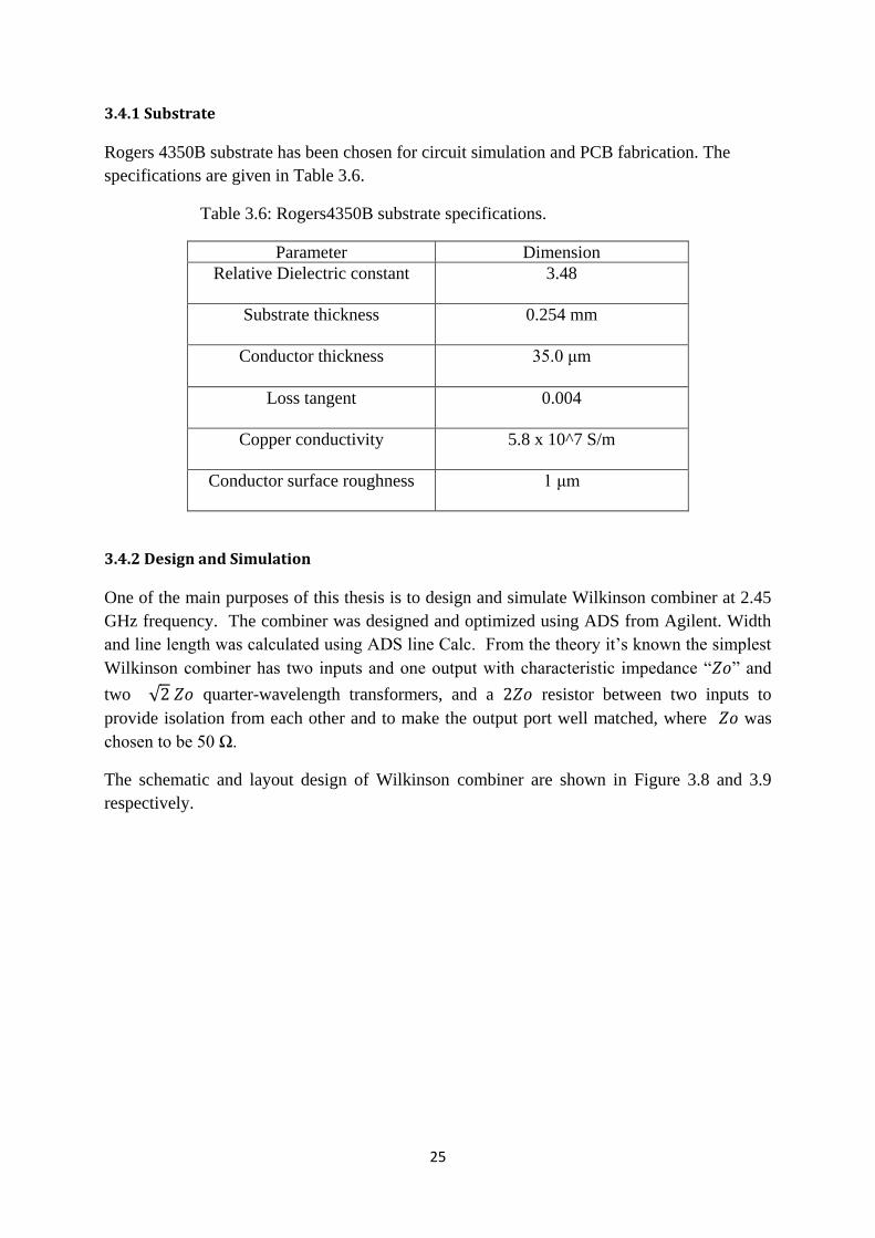
3.4.1 Substrate .............................................................................................................................. 25

3.4.2 Design and Simulation .......................................................................................................... 25

4 Prototype design and measurements ........................................................................... 28

4.1 Layout design ............................................................................................................................... 28

4.2 Prototype design ......................................................................................................................... 29

4.3 Measurement .............................................................................................................................. 30

4.3.1 Measurements using VNA .................................................................................................... 30

4.3.2 Measurements using ZigBee board ...................................................................................... 34

4.4 Measurement in reverberation chamber .................................................................................... 51

5 Results and discussions ................................................................................................... 52

5.1 Comparison between Fixed, Single, and Two Phases varied Average RSSI and Packet Error ..... 52

6 Conclusion and future work ............................................................................................ 58

6.1 Conclusion ................................................................................................................................... 58

6.2 Future work ................................................................................................................................. 58

7 References .......................................................................................................................... 59

1

1 Introduction

1.1 Background and motivation

In wireless communication, radio propagating in free space is regarded as the most ideal situation. However, in reality, propagation takes place around obstacles or even in atmosphere with gases, it will give rise to multipath propagation. Most signals are propagating in multipath environment. Considering mobile phone users, who moving around randomly in multipath environment, it will cause signal fading and received signal level variations over time. Diversity techniques have been used for solving this fading problem and being studied in mobile phones for a long time. There are many types of diversity, e.g. frequency, time, polarization, angle and space diversity (also as antenna diversity). When the channel is in the case of MIMO (multiple input multiple output), it implies that the antenna diversity can be employed at the transmitter side, which is provided with multiple copies of transmitted over two or more independent transmission channels [1], and can also be used at the received side, which means that each diversity branch then has its own receiver to the point where the branches are combined [2]. Antenna diversity can improve signals reliability only on the condition that the signals on the different branches are uncorrelated. However, in reality, correlation coefficient still exists. In this thesis, finding low correlation coefficient, through optimizing antenna diversity, is the first task.

All the existing diversity systems use multiple receiver or feedback systems, which are complex and costly. Now the time has come to use wireless sensor networks with a single receiver.

The goal of this thesis is to design antenna diversity system with opportunistic combining, this could be a new useful technique for mitigating fading beyond all existing systems because it can be easily implemented on transmit side as on receive side.

1.2 Problem description

The effect of antenna diversity is affected by the correlation between two antennas in the antenna diversity. In order to improve the signal reliability and enhance diversity gain, it is important to make correlation coefficient as low as possible through mounting two antennas in the different ways or placing two antenna in a further distance. The signal on branches should be combined in a clever way, so as to achieve maximum improvement in signal reliability while considering practical aspects.

1.3 Thesis outline

This thesis is divided into six chapters. The first chapter is the introduction part, including the project background and the problems which are investigated. The second chapter is regarding of the basic theories concerning about the project and these concepts are obtained from amount of references and books. In chapter three, design and simulation on software processes and results are presented, both on antenna diversity and phase shift. Chapter four is concerned about the prototype design and different measurements in reverberation chamber and office environments. In chapter five, measurement results are compared and discussed. The last chapter six, which is dealt with conclusion and future work.

2

2 Theoretical Background

2.1 Antenna theory

Antenna is an essential part of wireless communications. It is an electric and inherently bidirectional device that they can be used for either transmit or receive functions. An antenna can be viewed as a device that converts a guided electromagnetic wave on a transmission line to a plane wave propagating in the free space. Thus one side of an antenna appears as an electric circuit element, and the other side provides an interface with a propagating plane wave [3].

Radiation: When a time-varying and alternating voltage or current is applied to a

conductor, free electrons are accelerated in the space between atoms. The acceleration of

these electrons causes radiation to occur [4].

Far-Field region: A transmitting antenna is beyond the far-field distance df.. When D>>λ ,

it is expressed in equation 2.1 [1].

(2.1)

Radiation Pattern: The power density, S is not only dependent on the distance r, but also on the spherical coordinate angles θ and Φ, where θ denotes the angle in the zenith plane (azimuth) (0≤θ≤π), while Φ denotes the angle in the horizontal plane (0≤Φ≤βπ) [3]. Radiation pattern obtains from sketching S(θ,Φ) in the θ- or Φ- plane.

A typical radiation pattern is plotted in polar form, verse the angle Φ. The plot shows the relative variation of the radiated power of the antenna in dB, normalized to the maximum value [5]. As an example of Figure 2.1, the radiation pattern illustrated several distinct radiation lobes, which is presented maximum value in different directions [6]. The lobe having the maximum value is called the main lobe, while those lobes at lower level are called side lobes [5]. Side lobes are separated by nulls (no radiation in the null direction) [3].

Figure 2.1 Radiation pattern plotted in polar form.

3

Gain: The ratio of the maximum direction power density received from a given antenna to that of an isotropic radiator.

Directivity: The ratio of the maximum radiation intensity from a given antenna to the radiation intensity average over all space.

Radiation efficiency: It can be defined that the ratio of the desired output power to the supplied input power [5]. Since antenna power must induce loss, the relationship between the gain and directivity is [4].

(2.2)

When an antenna without any losses, i.e. ideal situation, there is 100% efficient and directivity is equal to gain. However, in practice, there are many parameters to contribute transmit power loss. One type is the external losses, such as impedance mismatch at the input to the antenna, or polarization mismatch with receive antenna, which can be eliminated by optimal circuit design. The other type of losses is due to the antenna itself, called resistive losses, resulting from metal conductivity and dielectric materials. Resistive losses remain in all antennas. The antenna radiation efficiency can be expressed as [7].

(2.3)

Where Prad is the radiated power by the antenna, Pin is the power supplied to the input of the antenna, and the Ploss is the power lost in the antenna, due to resistive losses [5]. The radiation efficiencies in antennas in mobile equipment are especially low, since the small electrical size of the terminals. Efficiencies of as low as 50% or even less are not uncommon [8].

Co-polarization: The polarization is what antenna is intended to radiate.

Cross-polarization: The polarization is orthogonal to co-polarization. For instance, if the polarization is Right Hand Circularly Polarization, the cross-polarization is Left Hand Circularly Polarization.

S-parameter: It is scattering parameters. In RF system, it defines the input-output relations of a network in terms of incident and reflected power waves [7]. Sij is obtained by driving the port j with an incident wave of voltage Vj

+, and measuring the reflected wave amplitude, Vi- ,

coming out of port i (the incident waves on all ports except the jth port are set to zero).

However, in a two antenna system, the two radios (radio 1 and radio 2) are regard as two ports (port 1 and port 2). Assuming that a1 and a2 are the incident waves on port 1 and port 2 respectively. Then b1 and b2 are the reflected waves from port1 and port 2 respectively.

4

The relationship can be described as follows.

1

1

2221

1211

2

1

a

a

SS

SS

b

b (2.4)

Where, S11 is the reflected power radio 1 which is attempting to deliver to antenna 1. S12 is the power from radio 2 is delivered to radio 1. S22 is the reflected power radio 2 which is attempting to deliver to antenna 2. In this case, S-parameter is a function of frequency. S11 is equal to input reflection coefficient which is looking from the source into the transmission line. So |S11| is as low as being regarded matching good.

VSWR: It is voltage standing wave ratio which is defined the ratio of the maximum voltage over the minimum voltage, ranging from 1 to infinite. It is a way to quantity the degree of mismatch. The ideal situation is VSWR=1, which means the termination is totally matched.

2.2 Planar inverted-F antenna

Planar inverted-F antennas have been increasingly common used for mobile phones. The antenna resonant is at quarter-wavelength. The size and radiation pattern make this type of antenna attractive. There are three main advantages:

1) a low profile, which can be built-in the handset mobiles. 2) omnidirectional radiation pattern, which exhibits moderate to high gain even in the polarization states, vertical and horizontal. 3) the finite ground plane leads to preferential radiation away from the user, which means that having reduced the backward radiation towards the user's head.

2.2.1 Planar inverted-F antenna structure

The basic PIFA consists of a top plate, a shorting pin, a feed wire and a ground, as shown in Figure 2.2.

5

Figure 2.2 Basic PIFA antenna structures.

In Figure 2.2, it shows that the PIFA with length L1, width L2, and the height h from the ground plate. The ground plate is a dielectric with relative permittivity ɛ >1 so the size can be reduced.

In general, the resonant frequency of PIFA can be approximate with [9]:

L1+L2+W = λ/4 (2.5)

where εf

cλ . c is the speed of light.

2 .3 Diversity System

Diversity techniques are used to improve the performance of data transmission over fading radio channels [1]. There are two types of fading, small-scale fading and large-scale fading. Diversity techniques, which solve the problem of small-scale fading, are over several branches (also called channels). These branches are uncorrelated fading channels to avoid the signals experience deep fades simultaneously.

There are many types of diversity, e.g. frequency, time, and space diversity and so on. In this thesis, space diversity is involved.

2.3.1 Antenna Diversity

Antenna diversity is one type of diversity, also called space diversity. In multipath propagation, placing receiving antennas at different locations will result in different received signal levels [1]. It requires antennas give uncorrelated signals, resulting from separating the antennas sufficiently large to decrease the correlation coefficients.

Nowadays, with modern wireless communications, the channel is MIMO, so space diversity can be employed both at the transmit and the receive side. So, Multiplicative order of diversity is obtained.

6

2.4 Correlation Coefficients

In antenna diversity, it assumes that if two antennas are separated large enough, the signals will be independent of each other, which means they are totally uncorrelated signals. However, in practical system, it hardly to achieve this ideal situation, maybe due to antennas mounted closely and other unknown losses. The correlation coefficient is a measure standard of how independent between antennas. The aim for antenna design is to make correlation coefficients, ranging from 0 to 1, as low as possible. When the correlation is equal to 0, it indicates perfectly uncorrelated antennas.

2.4.1 Calculating correlation from S-parameter

It is a simple but not accurate way if the radiation efficiencies of the antenna are low and the correlation of the losses are unknown. The following formula can be used to obtain correlation

2

21

2

22

2

21

2

11

21*22

*2111

11 SSSS

SSSS

(2.6)

The result retrieved from the simulation of antennas in HFSS and the antennas are simulated in free space.

2.4.2 Calculating correlation from radiation pattern

Correlation obtained from far-field is an accurate way either in free space or in a normal environment, where there are objects around to make signal scatter. The formulas are shown below.

(2.7)

(2.8)

(2.9)

Where, Ucp, 1 = Complex radiation in co-polarization from antenna 1

Uxp, 1 = Complex radiation in cross-polarization from antenna 1

Ucp, 2 = Complex radiation in co-polarization from antenna 2

Uxp, 2 = Complex radiation in cross-polarization from antenna 2

M

m

N

nnmnxpmncp UUP

1 1

2

1,

2

1,1 sin,,

M

m

N

nnmnxpmncp UUP

1 1

2

2,

2

2,2 sin,,

21

1 1

*2,1,

*2,1, sin,,,,

PP

UUUUM

m

N

nnmnxpmnxpmncpmncp

c

7

2.5 Diversity Gain

It is an effective approach to evaluate the antenna diversity. The lower correlation coefficients, the higher diversity gain. It can be defined as the increase in the power level where it has certain signal reliability, for constant SNR. Another way is to say the diversity gain is the improvement in time-averaged SNR from combined signals from a diversity antenna system, relative to the SNR from one signal system, preferably the best one [10]. The definition is specific requirement on the SNR above a reference level.

The general mathematical expression for diversity gain (DG) is as follows:

(dB) (2.10)

where けc is the instantaneous SNR of diversity combined signal, Γc is the mean SNR of the

combined signal, け1 is the highest SNR of the diversity branch signals, Γ1 is the mean value of

け1 and けs/ Γ is a threshold or reference level[11].

The e definition gain is illustrated in Figure 2.3. This will give a theoretical diversity gain is 7dB, because the change in average power is 3dB, the change in noise power is 0 dB, the change in outage level is 10dB, given in below Figure 2.3.

Figure 2.3 Diversity gain in with and without diversity situations.

The output probability is dependent on the M branches. Assuming the uncorrelated signals with Rayleigh distribution in the same average SNR branches, then the probability is expressed as follows [10]:

(2.11)

-30

-20

-10

0

10

20

Level (d

B)

Time-30

-20

-10

0

10

20

Level (d

B)

Time

8

2.6 Phase shifter

Phase shifter is a device which is used to adjust the phase angle of a system or a network when passing through it. Theoretically ideal phase shifter will provide very low insertion loss and some other loss but practically it’s not possible. A lot of parameters are related with it’s design and performance of the phase shifter like operating frequencies, insertion loss (IL), the limits of the phase change, switching speed, temperature sensitivity, return loss (RL), power handling (P) etc [12]. It can be controlled electrically, mechanically, or magnetically. There are different types of phase shifters like analog, digital, active, passive etc. It has numerous applications such as phase array antennas, beam forming modules, military radar, linearization of power amplifier, satellite communication etc.

2.6.1 Analog phase shifter

This is one part of this thesis works. It provides continuous variable phase shifts with the control input. It can be controlled both electrically and mechanically. The most commonly semiconductor control elements used in its design are varactor diodes which operate in reversed biased condition providing junction capacitance that varies with applied voltage or nonlinear dielectrics such as Barium Strontium Titanate, or Ferro-electric materials such as Yttrium iron garnet [12]. It provides monotonic (with monotonic means output always increases as the input increases) performance with high resolution. The main advantages of analog phase shifter are that it uses less area and provide large amount of phase shift range with low insertion loss, at low accuracy cost.

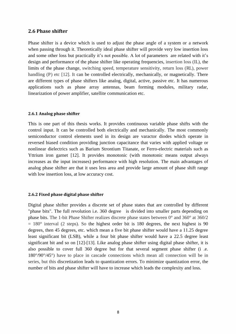
2.6.2 Fixed phase digital phase shifter

Digital phase shifter provides a discrete set of phase states that are controlled by different "phase bits". The full revolution i.e. 360 degree is divided into smaller parts depending on phase bits. The 1-bit Phase Shifter realizes discrete phase states between 0° and 360° at 360/2 = 180° interval (2 steps). So the highest order bit is 180 degrees, the next highest is 90 degrees, then 45 degrees, etc. which mean a five bit phase shifter would have a 11.25 degree least significant bit (LSB), while a four bit phase shifter would have a 22.5 degree least significant bit and so on [12]-[13]. Like analog phase shifter using digital phase shifter, it is also possible to cover full 360 degree but for that several segment phase shifter (i .e. 180°/90°/45°) have to place in cascade connections which mean all connection will be in series, but this discretization leads to quantization errors. To minimize quantization error, the number of bits and phase shifter will have to increase which leads the complexity and loss.

9

2.7 Relation between Propagation Constant, Phase Shift, Delay, and

Wavelength

The propagation constant or propagation coefficient in a transmission line is the complex number which comprise of real and imaginary parts. It determines the manner in which way the signal (voltage/current) will vary according to distance x. The real part is called attenuation constant (α, neper per unit length) which represents the reduction of signal (voltage/current) along the line where as the imaginary part is called phase constant (く, radians per unit length) which represents the variation of phase of signal along the line. The phase constant is denoted by

け = α + j く (2.12)

where, α = attenuation constant

く = phase constant

This is actually valid for loss line. For lossless line it will give purely imaginary part and will be proportional to the function of frequency.

Phase shift can be represented in degree or radians. One full wavelength is equal to 360° (or 2π radians) and as shown in figure 2.4 below.

Figure 2.4 Relationship between degree (°), radian (2π), phase shift (β), and wavelength (λ).

From the above figure, the relation between phases constant in βπ radian and wave length at a distance x is

く = (radian/length) (2.13)

π

2π

λ

β ふxぶ

Length x

180 360 90

10

Some other relations can be derived from the above Figure 2.4 [13]. As phase shift is also termed as delay so the relation between time delay and phase shift for transmission line is

Time delay (sec) = (2.14)

The phase velocity is termed for a single wave when travelling along a line at a certain frequency. It has an inverse relation with time delay is

Time delay (sec) = (2.15)

and group velocity is termed for at different frequencies with different velocities along the transmission line.

The group delay is the average delay of the various sinusoidal components while passing through a circuit or device under test.

The group delay has a proportional relation with rate of phase shift at certain frequency of interest.

Group delay (sec) = [ ] x [

] (2.16)

2.8 Phase varying conditions

Different phase varying conditions can be considered for opportunistic combining system which is discussed in below [14].

I. QUASI STATIC PHASE

Consider two signals at the antenna:

S1 = A1 cos (2.17a)

S2 = A2 cos (2.17b)

so, combined to received signal:

Sr = S1 + S2 = A1 cos + A2 cos (2.18)

The I channel is

Irx = 2 Sr cos ( = A1 cos + A2 cos (2.19a)

The Q channel is

Qrx = 2 Sr sin ( = - A1 sin - A2 sin (2.19b)

11

maximum will occurs when =

If a matched filter or integrate and dump detector is used on I and Q channel then:

= dt = Irx (2.20)

= Qrx (2.21)

II. TIME VARYING PHASE - VIEWPOINT 1 In this case is assumed to change linearly with time, and the period time T = Ts/n for an integer n 1

= t (2.22)

In this case the I and Q channels are:

Irx = 2 Sr cos ( = A1 cos + A2 cos (2.23)

Qrx = 2 Sr sin ( = - A1 cos - A2 cos (2.24)

Using an integrate and dump detector:

= dt = A2 cos (2.25)

= dt = - A2 sin (2.26)

If the phase sweep is an integer multiple of a complete sweep from 0 to 360 , the contribution from antenna 1 (where the phase sweep occurs) cancels completely if a integrate and dump detector is used. It is therefore unlikely the technique will work with common coherent receiver with integrate and dump detection.

12

III. TIME VARYING PHASE - VIEWPOINT 2 For a varying phase according to:

= t (2.27)

The total received signal is:

Sr = S1 + S2 = A1 cos + A2 cos = A1 cos t + A2 cos (2.28)

A linear increase in phase is the same as a frequency shift

f1 = =

(2.29)

hence

Sr = S1 + S2 = A1 cos + A2 cos (2.30)

This shows that when the phase on one antenna changes with time, the resulting received signal from the two antennas consists of two signals with different center frequencies. It may be predicted this will introduce problems for the carrier recovery circuit in a receiver. However, assuming A1 = A2 = A the received signal can also be written in the following form:

Sr = 2A [cos cos )] (2.31)

So there is an effective carrier: = (2.32)

and an additional time varying amplitude modulation (2.33)

hence

Sr =2 A cos ( ) (2.34)

if a carrier recovery circuit can look to then the I and Q channel after mixing are

=2 Sr cos ( A cos ( ) (2.35) =2 Sr sin( A sin ( ) (2.36)

but Am changes with time so Irx and Qrx are still modulated with a frequency f1/2.

13

2.9 Combining techniques

The signals on the different branches should be combined in a clever way, so as to achieve maximum improvement in signal reliability while considering practical aspects, otherwise diversity gain can be lost. There are different types of combining techniques. Different types of combing technique call for different type of diversity. The most popular techniques are

1. Selection Combining 2. Maximum Ratio Combining 3. Equal Gain Combining

2.9.1 Selection Combining (SC)

This is a very simple technique. The main principle is to select the strongest signal from the different branches signal according to some quality measurement, which can be e.g. signal level, power or signal to noise ratio, and ignores the other signals which means it only use one signal at a time [1]. As it selects the strongest signal, so maximum SNR is available at the output which helps to reduce the effect of fading in signals. The disadvantages of this system is that complicated equipment is required on each branch to monitor signals continuously to find out strongest signal, and also, the signals must be monitored at a rate faster than fading process. The arrangement for SC is shown in Figure 2.5.

Figure 2.5 Principle of selection combining method.

Channel 1

Channel 2

Channel N

TransmitterReceiver

SNRmonitor

Select maxSNR

14

2.9.2 Maximum Ratio Combining (MRC)

In this technique, all branches are simultaneously used to get the maximum SNR at the output. Each of the branch signals is weighted (w) with their instantaneous SNRs. The branches are co-phased and summed up to get the resultant signal. After weighting the incoming branches, co-phasing is the main challenge of this system. It needs weight updates and SNR estimation which make it complex design. A main problem of this system is that each branch of signal must have the same phase shift before combining [1]. The arrangement for MRC is shown in Figure 2.6.

Figure 2.6 Principle of maximum ratio combining.

2.9.3 Equal Gain Combining (EGC)

This is the modified version of MRC. In this technique, all the branches weights (w) are all set to constant value, and then signals are co-phased before combining [1]. The arrangement for MRC is shown in Figure 2.7.

Figure 2.7 Principle of equal gain combining.

Channel 1

Channel 2

Channel N

TransmitterReceiver

Co-

Ph

asi

ng

an

d S

um

ma

tion

W1

W2

WN

Channel 1

Channel 2

Channel N

TransmitterReceiver

Co-

Ph

asi

ng

an

d S

um

ma

tion

W1

W2

WN

W = SNRi

W = Constant

15

2.10 Opportunistic combining (OC)

Most of the existing diversity system requires signal sensing or feedback system but OC does not require any of those. The main advantages of this combining is that it can be easily implemented on transmit and receive sides. The arrangements are shown in Figure 2.8.

Figure 2.8 Opportunistic diversity (a) Transmit side (b) Receiver side.

Sweeping Control

Divider

Transmit Diversity

Combiner

Receive Diversity

Sweeping Control

16

3 Design and Simulation

3.1 Software tools

HFSS stands for High Frequency Structure Simulator. It is one of the most commercial tools to implement antenna design and other RF electronic circuit elements design. HFSS provides the accuracy, capacity, and the performance to engineers. The most outstanding advantage is the 3-D full-wave electromagnetic field and engineers can extract scattering matrix parameters. However, the backwards is requiring large amount of computer memory and simulation time.

Advance Designed System (ADS) is moment method based software which is used for Wilkinson combiner design, simulation, and overall layout design for fabrication.

MATLAB is used for figure drawing purposes.

3.2 Antenna design

The correlation coefficient is changed by the distance and angle between two antennas in antenna diversity. Generally, increasing the distance of two antennas, the isolation between them will be improved, and if the two antennas are polarized diversity, the level of uncorrelation is higher than any other angles. So the length of PCB board is changed by 50, 70, 90, 110 and 130 mm; and the width is fixed to 50 mm. The main goal of design antenna diversity among different PCB dimension is to find out the lowest correlation coefficient at 2.45 GHz, which is the first step to obtain successful measurement.

So the design topology is shown below, Figure 3.1

Figure 3.1The design topology.

Width

Len

gth

17

3.2.1 Antenna specification

In this thesis, Mica 2.4 GHz SMD Antenna (part number: A5645) is adopted. This antenna is

widely used in wireless devices, e.g. mobile phones, laptops, sensors and headsets etc. The

frequency is ranged from 2.4-2.5 GHz. There are two significant advantages are that the

maximum reflection is -11dB, which is below -10dB and the maximum VSRW is 1.8:1.

The product is shown below Figure 3.2.

Figure 3.2 Mica A5645.

The dimension of this PIFA is shown in Table 3.1.

Table 3.1: Dimension of Mica A5645 [16].

3.2.2 Design specification

The proposal design plan is implemented by HFSS. The substrate is used by FR4, the normally PCB material, relative permittivity is 4.4 and dielectric loss tangent is 0.02 given by HFSS material library. The height of substrate is 0.8 mm. Regarding of the shelf on antenna, it is assumed one type of FR4 is utilized (relative permittivity = 4, dielectric loss tangent = 0 at the frequency at 2.45 GHz). All metal sheets are assigned ‘Finite Conductivity’ boundary, this kind of boundary is modeled high conductivity metal. PCB ground is set to ‘Perfect E’, i.e. perfect electric conductor, so that creating ideal conditions for elements. ‘Air box’, shown in Figure 3.3 [a], is radiation boundary, which is made of ‘air’ so that far field information may be extract from the structure in free space. To obtain the best result, a cubic air boundary is defined with a distance of λ/4.

18

Figure 3.3 shows the antenna diversity design in HFSS. In [a], it is the whole version of the design, and the distance between the boundary of ‘airbox’ and antennas is so long that being modeled far field radiation. When hiding the ‘airbox’ in vision as presented in [b], the antenna diversity design is expanded to see clearly. Figure 3.3 [c] is the back side of the design.

[a]

[b]

[c]

Figure 3.3 Antenna diversity design on HFSS (a) with air box (b) without air box (c) the backside.

19

けSolution setupげ is another important stage in HFSS design. It will display the desired data in

the frequency response of the structure.

Solution Frequency 2.45 GHz

Maximum Number of Passes 22

Maximum Delta S 0.02

Sweep Type Interpolating Table 3.2: Analysis setup details.

Type Linear Step Start 2.2 GHz Stop 2.7 GHz

Step Size 0.01 GHz Table 3.3: Sweep details.

3.2.3 Simulation result from S-parameter

According to expression (2.6), calculating correlation coefficients from S-parameter needs S-parameters in the form of complex values, not in the decibel unit. After analyzing the design, in the ‘Create Modal Solution Data Report’, S-parameters versus frequencies is obtained, then exporting values to Matlab to calculate the correlation coefficients by equation (2.6).

The simulated magnitudes of correlation coefficient versus frequencies with different PCB dimensions show in the Figure 3.4, from (a) to (e), i.e. the length of PCB are 50, 70, 90, 110 and 130 mm. It is obvious in (a) that, when the two antennas are near together, the correlation is much higher than those with larger distance, reaching to above 0.55 at 2.2 GHz. The correlation coefficient must be below 0.5 is an advanced requirement and generally, correlation is regarded as quite low just below 0.2. When the length of PCB is getting larger, as seen in (b), (c), (d), (e), the correlation is decreased to below 0.15 in 2.45 GHz.

20

(a) (b)

(c) (d)

(e)

Figure 3.4 The magnitude of correlation coefficients with dimension of (a) 50 mm*50 mm (b) 50 mm*70 mm (c) 50 mm*90 mm (d) 50 mm*110 mm (e) 50 mm*130 mm.

As seen in Table 3.4, the correlation coefficients are presented in the complex value. It is obvious that as the length of PCB is equal to 70 mm and 130 mm, the correlation coefficients are the lowest. However, integrating the factors, e.g. the phase shifter size and combined

21

circuit, the dimension of PCB can be neither too small, nor too big. So it is decided to use 50 mm*90 mm.

PCB Dimension Correlation Coefficient 50 mm*50 mm 0.2001-0.1891i

50 mm*70 mm -0.0064-0.0829i

50 mm*90 mm -0.1244+0.0236i

50 mm*110 mm -0.1063+0.0668i

50 mm*130 mm -0.0249+0.0498i

Table 3.4: The value of correlation coefficient with different PCB dimension.

3.2.4 Simulation result from radiation pattern

Even though, correlation is calculated by S-parameter formula, the approach is not very accurate for unknown antenna losses. Therefore, after the size of PCB is confirmed, it is better to adopt radiation pattern formula to calculate once again.

Based on the formula (2.7) ~ (2.9), setting co-polarization and cross-polarization is the first thing. Because all radiation from antenna should be considered and it does not matter which pair of polarization was chosen, as long as they are orthogonal. For simplicity, using θ and φ is to be orthogonal components. The simulation is a function of phi, for a number of theta angles. The sweeping range of phi is from 0 to 360 degree and theta is from 0 to 180 degree. Both of them are cut by 10 degree in every step. The two antennas are assigned ‘antenna 1’ and ‘antenna β’ to simulate and analyze separately.

Figure 3.5 (a) (b) (c) (d) plot the radiation pattern in the polar from at frequency 2.45 GHz from antenna 1. Figure (a) and (b) are the real and image value of co-polarization radiation from antenna 1 respectively. (c) and (d) are the real and image part of cross-polarization radiation from antenna 2 respectively. So Ucp,1 is made up by the (a) and (b); Uxp,1 is made up by the (c) and (d).

22

(a) (b)

(c) (d)

Figure 3.5 Radiation patterns from antenna1 (a) real value in co-polarization (b) image value in co-

polarization (c) real value in cross-polarization (d) image value in cross-polarization.

The same step is used to simulate antenna 2. When simulating one antenna radiation pattern, the other antenna port must be forbidden to excite. The results are exported to Matlab in order to calculate the correlation coefficients by formula (2.7) to (2.9), and the correlation is -0.3537-0.0564i.

3.2.5 Compare

In ideal situation, if there are no losses, the correlation coefficients obtained from S-parameters and radiation patterns are the same. However, the radiation efficiencies result in uncertain parameters in the calculated received signal correlation, if the correlation between the losses is known, which is often the case [8], because even though design matching network to eliminate external losses, the internal resistant always remains in the system. Moreover, the coefficient of losses between the two antennas is uncertain and hard to measure its actual value. One paper is presented the relations for the effect of antenna efficiencies have on the calculated correlation in theory formulas [8].

23

Using S-parameters to calculate the correlation coefficients is a simple but not accurate way, unless antenna efficiencies are very high. Otherwise, the more losses in antenna system, the more deviations occur.

To simulate radiation patterns in full-sphere is a prefer method, because it is without uncertain parameters and contributes an accurate value.

3.3 Phase shifter simulation

3.3.1 Phase shifter specifications

In this thesis, Hittite SMT package analog phase shifter (part number: HMC928LP5E) has been adopted which is controlled via control voltage from 0 to + 13 volt. This is extensively used in EW receiver, Beam forming modules, test equipment, Satellite communications, Military radar etc. The frequency range is 2 - 4 GHz. It provides continuous variable phase shifts from 0 to 450 degrees with low phase error within the frequency range. It shows monotonic property with respect to control voltage. The dimension of phase shifter is (L x W) 5x5 mm. The functional diagram is shown in Figure 3.6 [15].

Figure 3.6 Functional diagram.

In this thesis, phase shifter directly bought and examined it and got the almost same values (phase in degree) at different control voltages what are given in product specifications sheet. The experimental values are shown in Table 3.5.

24

Table 3.5: Phase shifter measurement values at different control voltages.

Serial

No.

Control voltage

(Volt)

Phase shift

S21 (degree)

01 0 -0.20

02 1 82.2

03 1.14 89.9

04 2 132.6

05 3.07 179.5

06 4 -141.3

07 5.23 -90.5

08 6 -68.3

09 7 -36.3

10 8 -7

11 8.06 0

12 9 20.1

The graphical representation of phase shifter response at different control voltages is shown in Figure 3.7.

Figure 3.7 Phase shift vs Vctl.

3.4 Wilkinson combiner

Wilkinson combiner is a passive microwave component. It is a three-port network made up of micro strip transmission line and is used to combine power of antennas in a system or multiple transistors in an amplifier. Its construction is very simple. It uses quarter wave transmission line which can be easily fabricated on the PCB board with a simple resistor. The resistor provides isolation between two input ports and makes the output port well matched. The resistor does not dissipate power when use as a divider so theoretically it’s a lossless component, though practically there is some loss but it does not affect so much on the overall performance.

0 1 2 3 4 5 6 7 8 9-150

-100

-50

0

50

100

150

200

Control voltage (volt)

Pha

se s

hift

(de

gree

)

Vctl vs Phase shift

Phase response

25

3.4.1 Substrate

Rogers 4350B substrate has been chosen for circuit simulation and PCB fabrication. The specifications are given in Table 3.6.

Table 3.6: Rogers4350B substrate specifications.

Parameter Dimension Relative Dielectric constant 3.48

Substrate thickness 0.254 mm

Conductor thickness γ5.0 たm

Loss tangent 0.004

Copper conductivity 5.8 x 10^7 S/m

Conductor surface roughness 1 たm

3.4.2 Design and Simulation

One of the main purposes of this thesis is to design and simulate Wilkinson combiner at 2.45 GHz frequency. The combiner was designed and optimized using ADS from Agilent. Width and line length was calculated using ADS line Calc. From the theory it’s known the simplest Wilkinson combiner has two inputs and one output with characteristic impedance “ ” and two quarter-wavelength transformers, and a resistor between two inputs to provide isolation from each other and to make the output port well matched, where was chosen to be 50 Ω.

The schematic and layout design of Wilkinson combiner are shown in Figure 3.8 and 3.9 respectively.

26

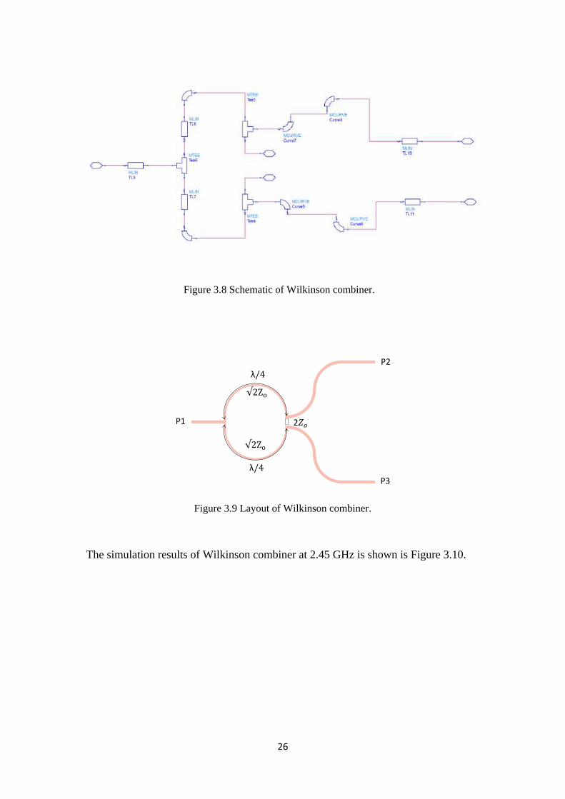
Figure 3.8 Schematic of Wilkinson combiner.

Figure 3.9 Layout of Wilkinson combiner.

The simulation results of Wilkinson combiner at 2.45 GHz is shown is Figure 3.10.

λ

λ

2 P1

P2

P3

27

Figure 3.10 Wilkinson combiner outputs (a) Input reflection, (b) Output reflection, (c) Forward transmission at port 2 and port 3, (d) Phase response at port 2 and port 3.

The simulation results show that they follow the principle of combiner i.e. they show the same amplitude and no phase difference, besides it shows -28.5 dB reflection at input port which is reasonable.

S11 S22

S21

S31 S21

S31

28

4 Prototype design and measurements

4.1 Layout design

The main task is to design antenna diversity system with opportunistic at 2.45 GHz center frequency. The design has divided three parts such as antenna section, phase shifter section, and combiner section. Though the antenna was simulated with HFSS but the overall layout part for PCB fabrication has been designed using ADS version 2011 and Rogers 4350B substrate is used for PCB fabrication.

The Layout design of antenna diversity system is shown in Figure 4.1.

(a) (b)

Figure 4.1 Layout design of antenna diversity system (a) without antennas (b) with antennas.

After layout design, PCB is manufactured in PCB lab which is shown in Figure 4.2 below.

Figure 4.2 Manufacture of PCB of antenna diversity system without components.

50 mm

90

mm

48 mm

48

mm

Antenna

section

Out put

Combiner section

Phase shifter section

29

4.2 Prototype design

After manufacturing of PCB, two prototypes, one with antenna and another without antenna have been made and 50 Ω SMA connectors were soldered to input and output ports to measure antenna parameters. All prototypes have been made in PCB lab at Linköping University. Though the main focus of this thesis to make a total integral prototype but another prototype without antenna is made for safety purpose. If main prototype wouldn’t work anyhow, then this extra part (without antenna prototype) could be used for measuring purpose but for this, two extra single antennas will have to add at input SMA connectors maintaining a reasonable distance with extra wire between antennas to get low co-relation coefficient but this will experience some losses due extra wire.

The prototype of without and with diversity systems are shown in below Figure 4.3 and 4.4 respectively.

Figure 4.3 Prototype of antenna diversity system without antennas.

Figure 4.4 Prototype of total antenna diversity system.

90 mm

50

mm

48 mm

48

mm

Edge mounted SMA connector

Phase shifters

PIFA antennas Vctl pins

30

Figure 4.5 Bottom view of total antenna diversity system.

One of the transmission lines from antenna to phase shifters is slightly zigzag (in Figure 4.4) than other so that it can avoid fringing effects from antenna during test. Two pins for DC signal of the phase shifters are placed on the opposite side so that they together with connecting cables (red cables shown in above Figure 4.5) will have less influence to the radiation tests.

4.3 Measurement

To measure prototype, different measurement configurations have been taken which are given below in different sections. Though two prototypes were made but finally total measurements only conducted with total integral prototype.

4.3.1 Measurements using VNA

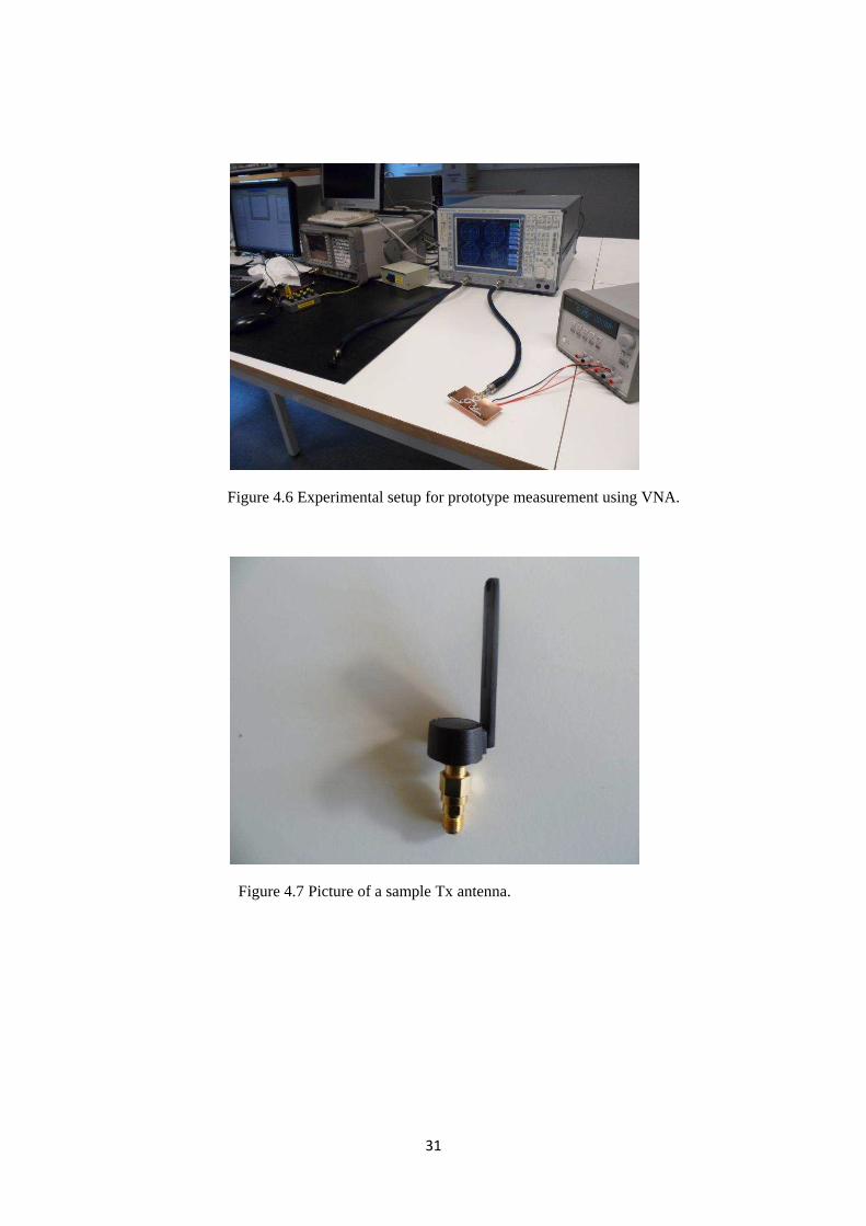
One port of Vector network analyzer (VNA) was connected with sample Tx antenna and another port of VNA with prototype PCB board. Regarding phase shifter, power supplied to the phase shifter for antenna 1 with a varying control voltage while keeping the other control voltage steady at 0 V. This gave the S21 values, which are the combined signals from both antennas. Then changed connection and varied the control voltage for antenna 2 while keeping the control voltage for antenna 1 fixed at 0 V. These also gave the S21 values to the right in the table, still the combined signals from both antennas. This measurement has been performed for three different sample antenna positions. The experimental set up for this measurement is shown in Figure 4.6.

90 mm

50

mm

31

Figure 4.6 Experimental setup for prototype measurement using VNA.

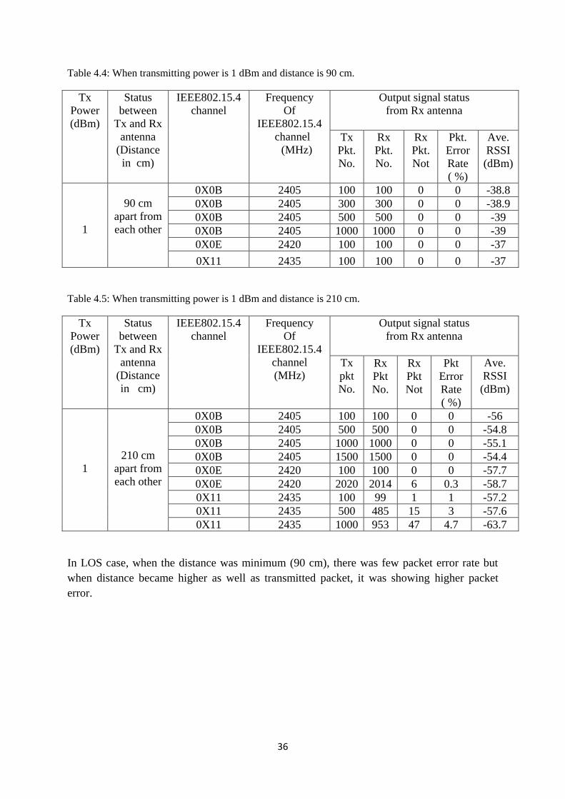
Figure 4.7 Picture of a sample Tx antenna.

32

The measurement values of S21 at different distances are given below in different tables.

Table 4.1: When the distance between Tx antenna and diversity antennas is 28 cm.

Serial No.


Combine output signal from prototype antennas

(When PS 1 is varied and PS 2 is fixed at 0 V)



S21 (degree)

S21 (dB)

Overall amplitude

varied (dB)

S21 (degree)

S21

(dB) Overall

amplitude varied (dB))

01 0 -48.21 -50.28

10.36

-86.37 -48.74

7.36

02 1 -72.14 -44.10 25.76 -52.68 03 2 -52.94 -41.83 86.39 -49.52 04 3 -40.94 -41.32 126.78 -47.21 05 4 -27.46 -42.11 160.89 -45.32 06 5 -13.27 -42.99 -169.14 -45.6 07 6 2.66 -45.29 -136.55 -46.17 08 7 -8.62 -49.52 -111.63 -47.18 09 8 -31.2 -52.47 -92.57 -47.99 10 9 -59.8 -50.23 -62.49 -49.22


Serial No.






S21 (degree)

S21 (dB)

Overall amplitude

varied (dB)

S21 (degree)

S21

(dB) Overall

amplitude varied (dB))

01 0 -30.91 -49.0

7.93

-52.19 -50.69

8.01

02 1 -54.10 -44.66 74.55 -46.99 03 2 -43.67 -42.29 105.11 -44.68 04 3 -32.30 -42.99 136.55 -42.68 05 4 -26.21 -42.10 155 -42.86 06 5 -13.81 -44.91 -154.60 -43.70 07 6 -2.32 -45.76 -142.37 -45.90 08 7 -13.78 -48.54 -109.22 -47.52 09 8 -23.84 -50.03 -74.16 -49.22 10 9 -43.80 -49.62 -19.35 -48.96

33


Serial No.






S21

(degree) S21

(dB) Overall

amplitude varied (dB)

S21 (degree)

S21 (dB)

Overall amplitude

varied (dB)

01 0 -19.04 -60.50

17.33

8.08 -59.80

9.11

02 1 -35.91 -51.78 137.36 -52.26 03 2 -18.44 -49.04 173.93 -52.99 04 3 -3.90 -48.35 -157.48 -50.76 05 4 15.44 -49.10 -128.51 -50.69 06 5 27.39 -48.99 -92.73 -51.88 07 6 52.37 -53.04 -72.16 -54.41 08 7 66.75 -57.31 -39.0 -58.17 09 8 22.48 -65.68 14.97 -58.30 10 9 -30.99 -63.06 50.11 -56.95

The above measurement values are represented graphically using matlab which are shown in Figure 4.3 and 4.4 respectively.

Figure 4.8 Variation of S21 values for diversity antennas at different control voltages.

0 1 2 3 4 5 6 7 8 9-70

-65

-60

-55

-50

-45

-40


S21

(dB

)

Vctl vs S21(when PS 1 is varied and PS 2 is fixed at 0 V)

S21 at 28 cmS21 at 35 cmS21 at 42 cm

34

Figure 4.9 Variation of S21 values for diversity antennas at different control voltages.

This measurement values imply that higher the distances, higher the signal variation.

4.3.2 Measurements using ZigBee board

ZigBee is a wireless communication protocol which is used for wireless personal area networks (WPANs) based on IEEE 802 standard. It is comparatively simpler, cheaper and stronger method than other WPANs method like Bluetooth. The ZigBee demo board uses QPSK modulation signal and measures the link quality under real circumstances. The demo board can directly measure RSSI and Packet error rate. Smart RF studio 7 software tools from Texas Instruments Inc. assisted to record RSSI and Packer error rate parameter values. Two demo boards were connected with two PCs and one acted as a Tx and another as a Rx. The measurement performed for different power level at different distances including in LOS (Line Of Sight) environment and close environment (with close mean concrete wall barrier between Tx and Rx). Different experimental configuration were performed which are given below.

4.3.2.1 When single antenna as a Tx and single antenna as a Rx

Two pieces of single antenna were taken and one used as Tx and another used as Rx. The measurements were performed in LOS. Figure 4.5 and 4.6 shows the picture of ZigBee board and monitor window and measurement values are given in below different tables.

0 1 2 3 4 5 6 7 8 9-60

-58

-56

-54

-52

-50

-48

-46

-44

-42


S21

(dB

)

Vctl vs S21(when PS 2 is varied and PS 1 is fixed at 0 V)

S21 at 28 cmS21 at 35 cmS21 at 42 cm

35

Figure 4.10 Picture of ZigBee demo board .

Figure 4.11 RSSI and Packer error rate parameters monitor window.

36

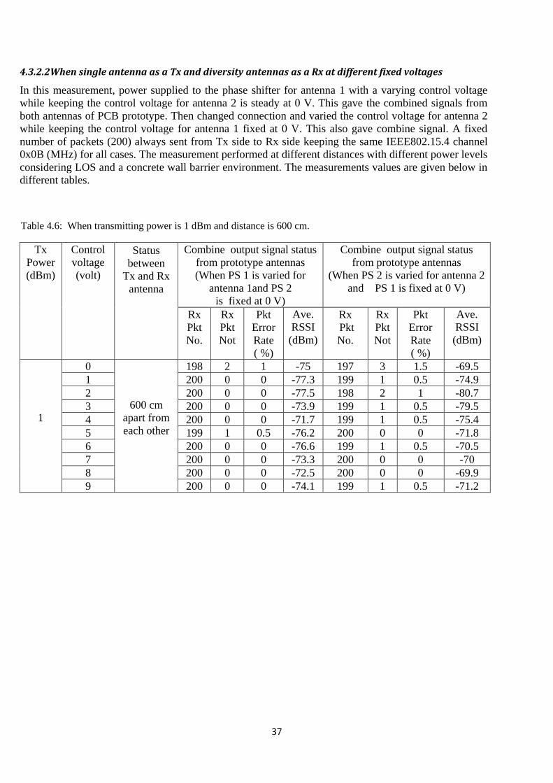
Table 4.4: When transmitting power is 1 dBm and distance is 90 cm.

Tx Power (dBm)

Status between

Tx and Rx antenna

(Distance in cm)

IEEE802.15.4 channel

Frequency Of

IEEE802.15.4 channel (MHz)

Output signal status from Rx antenna

Tx Pkt. No.

Rx Pkt. No.

Rx Pkt. Not

Pkt. Error Rate ( %)

Ave. RSSI (dBm)

1

90 cm

apart from each other

0X0B 2405 100 100 0 0 -38.8 0X0B 2405 300 300 0 0 -38.9 0X0B 2405 500 500 0 0 -39 0X0B 2405 1000 1000 0 0 -39 0X0E 2420 100 100 0 0 -37

0X11 2435 100 100 0 0 -37


Tx Power (dBm)

Status between

Tx and Rx antenna

(Distance in cm)

IEEE802.15.4 channel

Frequency Of

IEEE802.15.4 channel (MHz)

Output signal status from Rx antenna

Tx pkt No.

Rx Pkt No.

Rx Pkt Not

Pkt Error Rate ( %)

Ave. RSSI (dBm)

1

210 cm apart from each other

0X0B 2405 100 100 0 0 -56 0X0B 2405 500 500 0 0 -54.8 0X0B 2405 1000 1000 0 0 -55.1 0X0B 2405 1500 1500 0 0 -54.4 0X0E 2420 100 100 0 0 -57.7 0X0E 2420 2020 2014 6 0.3 -58.7 0X11 2435 100 99 1 1 -57.2 0X11 2435 500 485 15 3 -57.6 0X11 2435 1000 953 47 4.7 -63.7

In LOS case, when the distance was minimum (90 cm), there was few packet error rate but when distance became higher as well as transmitted packet, it was showing higher packet error.

37

4.3.2.2When single antenna as a Tx and diversity antennas as a Rx at different fixed voltages

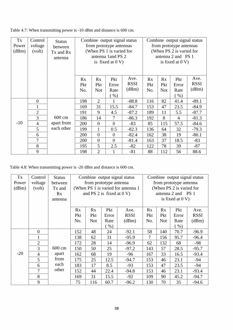
In this measurement, power supplied to the phase shifter for antenna 1 with a varying control voltage while keeping the control voltage for antenna 2 is steady at 0 V. This gave the combined signals from both antennas of PCB prototype. Then changed connection and varied the control voltage for antenna 2 while keeping the control voltage for antenna 1 fixed at 0 V. This also gave combine signal. A fixed number of packets (200) always sent from Tx side to Rx side keeping the same IEEE802.15.4 channel 0x0B (MHz) for all cases. The measurement performed at different distances with different power levels considering LOS and a concrete wall barrier environment. The measurements values are given below in different tables.


Tx Power (dBm)


Status between

Tx and Rx antenna

Combine output signal status from prototype antennas (When PS 1 is varied for

antenna 1and PS 2 is fixed at 0 V)

Combine output signal status from prototype antennas

(When PS 2 is varied for antenna 2 and PS 1 is fixed at 0 V)

Rx Pkt No.

Rx Pkt Not

Pkt Error Rate ( %)

Ave. RSSI (dBm)

Rx Pkt No.

Rx Pkt Not

Pkt Error Rate ( %)

Ave. RSSI (dBm)

1

0


198 2 1 -75 197 3 1.5 -69.5 1 200 0 0 -77.3 199 1 0.5 -74.9 2 200 0 0 -77.5 198 2 1 -80.7 3 200 0 0 -73.9 199 1 0.5 -79.5 4 200 0 0 -71.7 199 1 0.5 -75.4 5 199 1 0.5 -76.2 200 0 0 -71.8 6 200 0 0 -76.6 199 1 0.5 -70.5 7 200 0 0 -73.3 200 0 0 -70 8 200 0 0 -72.5 200 0 0 -69.9 9 200 0 0 -74.1 199 1 0.5 -71.2

38

Table 4.7: When transmitting power is -10 dBm and distance is 600 cm.

Tx Power (dBm)


Status between

Tx and Rx antenna




antenna 2 and PS 1 is fixed at 0 V)

Rx Pkt No.

Rx Pkt Not

Pkt Error Rate ( %)

Ave. RSSI (dBm)

Rx Pkt No.

Rx Pkt Not

Pkt Error Rate ( %)

Ave. RSSI (dBm)

-10

0


198 2 1 -88.8 116 82 41.4 -89.1 1 169 31 15.5 -84.7 153 47 23.5 -84.9 2 191 9 4.5 -87.2 189 11 5.5 -87.7 3 186 14 7 -86.3 192 8 4 -81.3 4 200 0 0 -83 85 115 57.5 -84.6 5 199 1 0.5 -82.3 136 64 32 -79.3 6 200 0 0 -82.4 162 38 19 -80.1 7 200 0 0 -81.4 163 37 18.5 -83 8 195 5 2.5 -82 122 78 39 -87 9 198 2 1 -81 88 112 56 88.6


Tx Power (dBm)


Status between Tx and

Rx antenna

Combine output signal status from prototype antenna


Combine output signal status from prototype antenna (When PS 2 is varied for


Rx Pkt No.

Rx Pkt Not

Pkt Error Rate ( %)

Ave. RSSI (dBm)

Rx Pkt No.

Rx Pkt Not

Pkt Error Rate ( %)

Ave. RSSI (dBm)

-20

0


152 48 24 -92.1 58 140 70.7 -96.9 1 138 62 31 -95.9 7 156 95.7 -96.4 2 172 28 14 -96.9 62 132 68 -98 3 150 50 25 -97.2 143 57 28.5 -95.7 4 162 68 19 -96 167 33 16.5 -93.4 5 175 25 12.5 -94.7 153 46 23.1 -94 6 183 17 8.5 -93 153 47 23.5 -94 7 152 44 22.4 -94.8 153 46 23.1 -93.4 8 169 31 15.5 -92 109 90 45.2 -94.7 9 75 116 60.7 -96.2 130 70 35 -94.6

39

Table 4.9: When transmitting power is -10 dBm and Concrete wall barrier between them.

Tx Power (dBm)


Status between

Tx and Rx antenna





Rx Pkt No.

Rx Pkt Not

Pkt Error Rate ( %)

Ave. RSSI (dBm)

Rx Pkt No.

Rx Pkt Not

Pkt Error Rate ( %)

Ave. RSSI (dBm)

-10

0

600 cm apart from

each Other and

Concrete wall

barrier between

them

138 68 30.7 -94.8 166 34 17 -86.8

1 192 8 4 -89.5 173 27 13.5 -91 2 198 2 1 -89 179 21 10.5 -90.7

3 199 1 0.5 -91.2 130 70 3.5 93.4

4 188 12 6 -92.9 175 7 12.5 -88.7

5 164 35 17.6 -95.1 198 2 1 -85

6 174 25 12.6 -94.6 184 16 8 -85.1

7 182 18 9 -93 190 10 5 -85 8 167 33 16.5 -93 198 2 1 -85 9 171 29 14.5 -91.2 192 8 4 -85.6


Tx Power (dBm)


Status between Tx and Rx antenna





Rx Pkt No.

Rx Pkt Not

Pkt Error Rate ( %)

Ave. RSSI (dBm)

Rx Pkt No.

Rx Pkt Not

Pkt Error Rate ( %)

Ave. RSSI (dBm)

-14

0 600 cm

apart from each Other and

Concrete wall

barrier between

them

140 59 29.6 -97.4 161 34 17.4 -93.9 1 159 41 20.5 -93.6 151 45 23 -93.2 2 184 16 8 -95.1 140 57 28.9 -94.8 3 55 138 71.5 -98.1 135 63 31.8 -96.3 4 147 51 25.8 -97.5 11 81 88 -98.4

5 169 31 15.5 -96.1 No

value No value

No v alue

No value

6 15 29 65.9 -97.3 90 109 54.8 -98.3 7 166 32 16.2 -97.4 127 73 36.5 -95.6 8 151 49 24.5 -98 156 44 22 -93.3 9 143 56 28.1 -95.5 155 45 22.5 -93.6

40


Tx Power (dBm)


Status between

Tx and Rx antenna





Rx Pkt No.

Rx Pkt Not

Pkt Error Rate ( %)

Ave. RSSI (dBm)

Rx Pkt No.

Rx Pkt Not

Pkt Error Rate ( %)

Ave. RSSI (dBm)

-18

0

600 cm apart from

each Other and

Concrete wall

barrier between

them

2 35 94.6 -99 No

value No

value No

value No

value 1 76 124 62 -98.4 84 116 58 -98.7 2 176 24 12 -96.1 170 30 15 -96.4 3 43 69 61.6 -98.7 132 67 33.7 -98.1 4 41 71 59.6 -98 8 157 95.2 -98.8 5 40 70 61 -98.2 10 64 86.5 -99

6 63 126 66.7 -98.9 No

value No

value No

value No

value

7 54 144 72.7 -98.7 No

value No

value No

value No

value 8 156 42 21.2 -97.1 17 27 61.4 -98.9

9 149 51 25.5 -97.9 No

value No

value No

value No

value

In both LOS and close environment, when power was high and distance was minimum, packet error rate and signal strength was reasonable, but both were deteriorating with higher distances and low power. However, LOS provides better performance than close environment. Some cases, it didn’t show any data (No value) due weak signal which means data didn’t transfer successfully from Tx to Rx.

41

The graphical representation of above measurement results using matlab are shown in Figure 4.12 and

4.13 respectively.

Figure 4.12 Variation of RSSI values for diversity antennas at different control voltages in LOS

environment.

Figure 4.13 Variation of RSSI values for diversity antennas at different control voltages in close

environment.

0 1 2 3 4 5 6 7 8 9-100

-95

-90

-85

-80

-75

-70


RS

SI (

dBm

)

Vctl vs RSSI at different power level for LOS environment

AVG. RSSI at -1 dBmAVG. RSSI at -10 dBmAVG. RSSI at -20 dBm

0 1 2 3 4 5 6 7 8 9

-100

-98

-96

-94

-92

-90

-88


RS

SI (

dBm

)

Vctl vs RSSI at different power level for close environment


42

4.3.2.3 When single antenna as a Tx and diversity antennas as a Rx and single phase is varied with

different Functional generator signal

In this measurement, Signal supplied to the phase shifter for antenna 1 with varying signal generated by Functional generator while keeping the control voltage for antenna 2 is steady at 0 V. This gave the combined signals from both antennas of PCB prototype. Then changed and varied the signal for antenna 2 while keeping the control voltage for antenna 1 fixed at 0 V. The rest of the conditions are same as mentioned for above measurements. The measurements values are given below in different tables.


Tx Power (dBm)

Functional Generator Signal (KHz)

Status between Tx and Rx antenna





Rx Pkt No.

Rx Pkt Not

Pkt Error Rate ( %)

Ave. RSSI (dBm)

Rx Pkt No.

Rx Pkt Not

Pkt Error Rate ( %)

Ave. RSSI (dBm)

1

50


199 1 0.5 -73.2 199 1 0.5 -71 100 199 1 0.5 -76.2 200 0 0 -70.1 150 199 1 0.5 -74.2 199 1 0.5 -71.6 200 165 34 17.1 -73.2 163 36 18.1 -70.4 250 185 15 7.5 -77.9 200 0 0 -73.6 300 197 3 1.5 -80.2 199 1 0.5 -73.1 350 191 9 4.5 -81 199 1 0.5 -73.8 400 103 61 37.2 -81 199 1 0.5 -72.8 450 188 12 6 -81.7 130 70 35 -74 500 162 38 19 -78.1 82 115 58.4 -74.9 550 198 2 1 -79.7 137 63 31.5 -72.9 600 198 2 1 -76.7 191 9 4.5 -73.8

43


Tx Power (dBm)

Functional Generator

Signal (KHz)

Status between

Tx and Rx antenna





Rx Pkt No.

Rx Pkt Not

Pkt Error Rate ( %)

Ave. RSSI (dBm)

Rx Pkt No.

Rx Pkt Not

Pkt Error Rate ( %)

Ave. RSSI (dBm)

-10

50


189 11 5.5 -85.3 194 6 3 -85.4 100 199 1 0.5 -87 188 12 6 -86.2 150 171 29 14.5 -89 177 23 11.5 -87.3 200 163 37 18.5 -88.8 153 46 23.1 -90.2 250 96 104 52 -91.5 130 33 20.2 -90.2 300 1 22 95.7 -92 140 59 29.6 -90.6 350 1 34 97.1 -93 177 23 11.5 -90.2 400 30 169 84.9 -90.4 134 64 32.3 -89.8 450 183 17 8.5 -83.2 170 30 15 -89 500 176 16 8.3 -83.1 184 16 8 -89 550 6 154 96.2 -86.2 152 48 24 -89.8


Tx Power (dBm)


Signal (KHz)

Status between

Tx and Rx antenna





Rx Pkt No.

Rx Pkt Not

Pkt Error Rate ( %)

Ave. RSSI (dBm)

Rx Pkt No.

Rx Pkt Not

Pkt Error Rate ( %)

Ave. RSSI (dBm)

-20

50


14 172 92.5 -92.8 55 143 75.3 -97.9 100 33 160 82.9 -93.3 146 50 25.5 -95.4 150 15 154 91.1 -93.5 10 140 93.3 -97.6 200 68 129 65.5 -92.4 1 21 95.5 -94 250 89 93 51.1 -91.7 15 167 91.8 -95.9 300 98 91 48.1 -95 19 180 90.5 -94.8 350 15 99 86.8 -94.6 36 154 81.1 -94.7 400 160 33 17.1 -94.5 15 160 91.4 -95.5 450 147 42 22.2 -96 31 148 82.7 -97.9

500 No

value No

value No

value No

value 28 120 81.1 -98.1 550 4 118 96.7 -96.5 9 46 83.6 -97 600 No

value No

value No

value No

value 54 134 71.3 -97.1

44


Tx Power (dBm)


Signal (KHz)

Status between

Tx and Rx antenna





Rx Pkt No.

Rx Pkt Not

Pkt Error Rate ( %)

Ave. RSSI (dBm)

Rx Pkt No.

Rx Pkt Not

Pkt Error Rate ( %)

Ave. RSSI (dBm)

-10

50 600 cm

apart from each Other and

Concrete wall

barrier between

them

187 13 6.5 -87.1 107 93 46.5 -88.1 100 151 49 24.5 -88 93 105 53 -86.9 150 128 72 36 -88.9 37 157 80.9 -89.4 200 143 57 28.5 -88.9 38 157 80.5 -89.6 250 138 62 31 -89 17 170 90.9 -91.1 300 136 64 32 -88.7 12 149 92.5 -89.6

350 109 91 45.5 -89.3 No

value No

value No

value No

value 400 65 133 67.2 -90.5 7 41 85.4 -91.1 450 121 79 39.5 -89.6 4 133 97.1 -90.8 500 171 29 14.5 -87.3 1 17 94.4 -91


Tx Power (dBm)


Signal (KHz)

Status between

Tx and Rx antenna





Rx Pkt No.

Rx Pkt Not

Pkt Error Rate ( %)

Ave. RSSI (dBm)

Rx Pkt No.

Rx Pkt Not

Pkt Error Rate ( %)

Ave. RSSI (dBm)

-14

50

600 cm apart from

each Other and

Concrete wall

barrier between

them

74 125 62.8 -92.4 121 79 39.5 -92.7 100 119 81 40.5 -89.5 164 35 17.6 -93.3 150 95 103 52 -91.6 93 106 53.3 -95.4 200 96 104 52 -91.5 172 28 14 -90 250 72 127 63.8 -92.6 28 156 84.8 -91.2 300 45 145 76.3 -92.8 11 147 93 -91.1

350 69 131 65.5 -92.5 No

value No

value No

value No

value

400 53 146 73.4 -93.6 No

value No

value No

value No

value

450 71 82 53.6 -91.6 No

value No

value No

value No

value 500 80 117 59.4 -92.5 1 4 80 -91

550 32 168 84 -94.8 No

value No

value No

value No

value 600

47 142 75.1 -93.2 No

value No

value No

value No

value

45


Tx Power (dBm)


Signal (KHz)

Status between

Tx and Rx antenna





Rx Pkt No.

Rx Pkt Not

Pkt Error Rate ( %)

Ave. RSSI (dBm)

Rx Pkt No.

Rx Pkt Not

Pkt Error Rate ( %)

Ave. RSSI (dBm)

-18

50 600 cm apart from each Other

and Concrete

wall barrier between

them

78 113 59.2 -94.9 156 44 22 -94.1 100 65 132 67 -95.7 167 33 16.5 93.1 150 69 130 65.3 -94.5 172 28 14 -92.7 200 47 150 76.1 -94.9 158 41 21 -93.2 250 28 162 85.3 -96.8 44 150 77.3 -92.9 300 28 166 85.6 -95.5 22 171 88.6 -92.7 350 30 159 84.1 -95.7 4 71 94.7 -94 400 33 166 83.4 -95.6 No value No value No value No value 450 82 116 58.6 -95.9 No value No value No value No value 500 65 126 66 -94 No value No value No value No value 550 74 126 63 -95.6 No value No value No value No value 600 29

165

85.1

-98.2

No value

No value

No value

No value

The graphical representation of above measurement results using matlab are shown in Figure 4.14 and 4.15 respectively.

Figure 4.14 Variation of RSSI values for diversity antennas at different FG signals in LOS environment.

50 100 150 200 250 300 350 400 450 500 550-100

-95

-90

-85

-80

-75

-70


RS

SI (

dBm

)

FG signal vs RSSI at different power level for LOS environment


46

Figure 4.15 Variation of RSSI values for diversity antennas at different FG signals in close environment.

4.3.2.4 When single antenna as a Tx and diversity antennas as a Rx and two phases are varied

with different Functional generator signal

In this measurement, extra 3 Functional Generators (FG) and 1 Oscilloscope have been engaged. 2 FG used as slave and 1 FG is used as a Master which produced synchronized signal for triggering the slave. Before start to sweeping both phase, two outputs of slaves were connected to the Oscilloscope to check the stability between two slave signals and adjust a fixed phase shift (almost 90 depending on phase shifter control voltage from PS data sheet) between them through changing offset value from FGs and then disconnected slaves output from the Oscilloscope and connected with two phase shifter control pin from developed prototype diversity antennas. Repeated this procedure at different experimental frequencies. Figure 4.6 shows experimental set up for this measurement and FG displays setting and measurements values are given below in different tables.

Table 4.18: Different parameter setting at Functional Generator.

Display Modify Setting Trigger Mode Master Slave1 Slave2

Gated AMPL (V) 3.9 AMPL (V) 3.9 AMPL (V) 3.9 OFST (V) 2.5 OFST (V) 3.5 OFST (V) 2.5 SYM (%) 20 SYM (%) 20 SYM (%) 20

50 100 150 200 250 300 350 400 450 500-98

-96

-94

-92

-90

-88

-86


RS

SI (

dBm

)

FG signal vs RSSI at different power level for close environment


47

Figure 4.16 Experimental set up for two phase varying condition with FGs.

Figure 4.17 Close view of slaves stable output at Oscilloscope.

Master

Slave

48

Table 4.19: When transmitting power is 1 dBm and distance between Tx and Rx is 600 cm.

Tx

Power (dBm)


Signal as Master (SYNC Signal) (KHz)

Combine two Functional Generator

Signal as Slave

(Triggering Signal) (KHz)

Ave. RSSI (dBm)

Tx pkt No.

Rx Pkt No.

Rx Pkt Not

Pkt Error Rate ( %)

1

100 101 -64.4 200 200 0 0

200 220 -66.8 200 199 1 0.5

250 270 -66 200 74 110 59.8

300 330 -66 200 25 160 86.5

350 380 No value 200 No value No value No value

400 430 No value 200 0 10 100


500 540 No value 200 0 1 100

Table 4.20: When transmitting power is -10 dBm and distance between Tx and Rx is 600 cm.

Tx

Power (dBm)

Functional Generator Signalas Master

(SYNC Signal) (KHz)


Signalas Slave (Triggering Signal)

(KHz)

Ave. RSSI (dBm)

Tx pkt No.

Rx Pkt No.

Rx Pkt Not

Pkt Error Rate ( %)

-10

100 101 -77.5 200 200 0 0

200 220 -75.4 200 200 0 0

250 270 -76.3 200 75 118 61.1

300 330 -78 200 24 171 87.7


400 430 No value 200 0 1 100

450 490 No value 200 0 1 100


49


Tx

Power (dBm)


Signal as Master (SYNC Signal) (KHz)


Signal as Slave


Ave. RSSI (dBm)

Tx pkt No.

Rx Pkt No.

Rx Pkt Not

Pkt Error Rate ( %)

– 20

100 101 -88.6 200 193 7 3.5

200 220 -88.2 200 188 12 6

250 270 -88.2 200 68 126 64.9

300 330 -90.3 200 31 169 84.5

350 380 -89 200 1 1 50

400 430 No value 200 0 6 100

450 490 No value 200 0 3 100

500 540 No value 200 0 4 100


Tx

Power (dBm)

Functional Generator Signal

as Master (SYNC Signal)

(KHz)

Combine two Functional

Generator Signal as Slave


Ave. RSSI (dBm)

Tx pkt No.

Rx Pkt No.

Rx Pkt Not

Pkt Error Rate ( %)

– 10

100 101 -88.8 200 179 21 10.5

200 220 -90.9 200 183 17 8.5

250 270 -93.6 200 42 155 78.7

300 330 -96 200 1 5 83.3


400 430 No value 200 0 1 100


500 540 No value 200 0 1 100

50


Tx

Power (dBm)

Functional Generator Signalas Master

(SYNC Signal) (KHz)


Signalas Slave (Triggering

Signal) (KHz)

Ave. RSSI (dBm)

Tx pkt No.

Rx Pkt No.

Rx Pkt Not

Pkt Error Rate ( %)

-14

100 101 No value 200 0 15 100

200 220 -96.5 200 4 133 97.1

250 270 No value 200 0 2 100

300 330 -98 200 1 2 66.7






Tx Power (dBm)


Signalas Master (SYNC Signal)

(KHz)

Combine two Functional

Generator Signal as Slave


Ave. RSSI (dBm)

Tx pkt No.

Rx Pkt No.

Rx Pkt Not

Pkt Error Rate ( %)

-18

100 101 -98 200 21 168 88.9

200 220 -98 200 1 14 93.3

250 270 No value 200 0 10 100

300 330 No value 200 0 4 100




500 540 No value 200 0 2 100

51

4.4 Measurement in reverberation chamber

Reverberation Chamber (RC) is used for measurement purpose. The reverberation chamber was chosen for measurement had the dimension about 1x1x1.5 m.

First a monopole antenna was measured in the RC, but showed very high error rates. After placing absorbers in the RC the error rates dropped to levels similar to the ones measured in real environments measured data. The error rates were very steady in the RC over several measurements. Probably presence of high Q-factor in the RC which gave ISI due to long ringing is one reason.

Second, the diversity antennas (developed prototype) were measured in the same way in RC like monopole. Swept the control voltage at different frequencies (10, 62.5, 125, 250, 500 kHz). The measurement was conducted with both triangle and sinus curves with the help of hardware attenuators and the software to make sure the RSSI was the same as in the monopole measurements. Observed the comparison between diversity antennas and monopole were at different RSSI values. The results showed some small variations over several measurements. The average error rates were however about the same as with the monopole. In some cases there was a small improvement.

In order to check the signal environment in the RC more carefully, passive transmission measurements (S21) was tested in the RC, both with the monopole and with developed diversity antennas and with/without pieces of absorbers in the RC. Without absorbers, it was seen that a nice Rayleigh fading signal, however, with absorbers the S21 level went down, and there were fewer and not so deep fading dips, so the signal variations were not exactly Rayleigh. The curve was also not so smooth but edgy, which was an indication that there were too few waves in the RC. This means that the diversity technique was not tested in a good way in the RC with absorbers. Without absorbers the signal environment was too resonant, and with absorbers it was too sparse.

From this measurement it is difficult to draw any definite conclusion in sparse environment because the diversity technique seems to give neither an improvement nor degradation (perhaps sometimes a small improvement), compared with monopole antenna. And ‘sparse environment’ is a vague definition; it would be unlikely that accidentally obtain the same performance in specific environment if the richness was important.

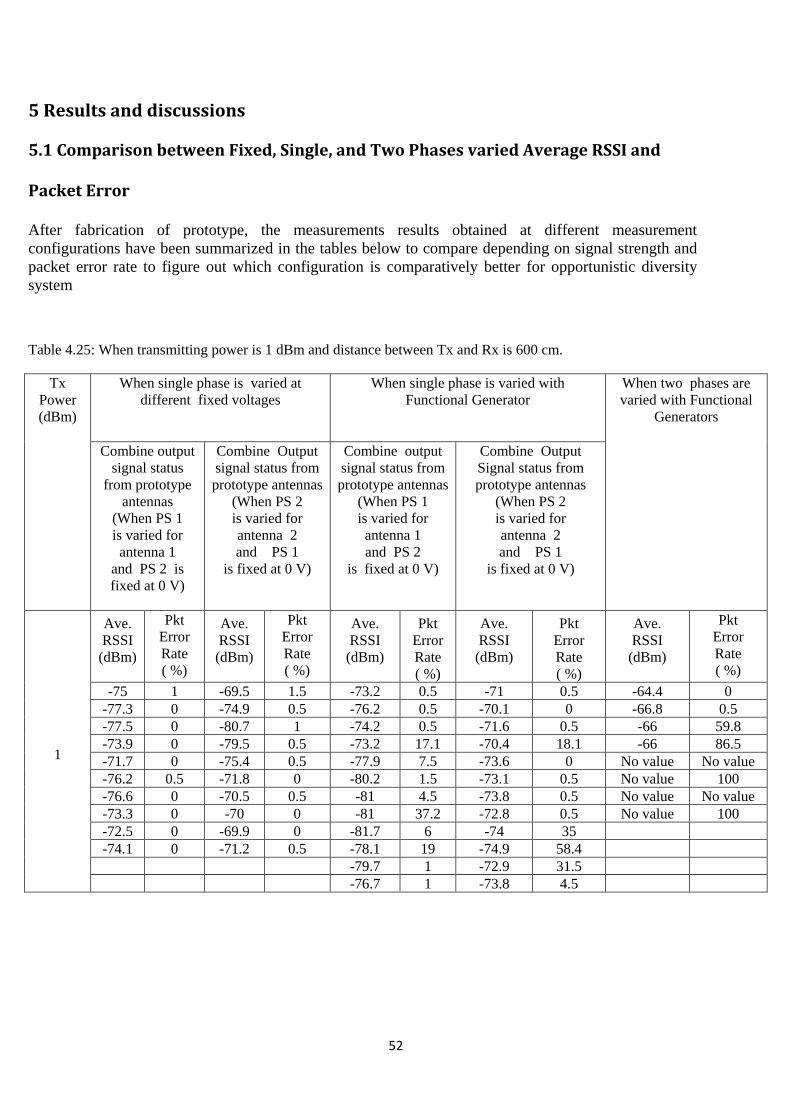
52

5 Results and discussions

5.1 Comparison between Fixed, Single, and Two Phases varied Average RSSI and

Packet Error

After fabrication of prototype, the measurements results obtained at different measurement configurations have been summarized in the tables below to compare depending on signal strength and packet error rate to figure out which configuration is comparatively better for opportunistic diversity system

Table 4.25: When transmitting power is 1 dBm and distance between Tx and Rx is 600 cm.

Tx Power (dBm)

When single phase is varied at different fixed voltages

When single phase is varied with Functional Generator

When two phases are varied with Functional

Generators

Combine output signal status

from prototype antennas

(When PS 1 is varied for antenna 1

and PS 2 is fixed at 0 V)

Combine Output signal status from prototype antennas

(When PS 2 is varied for antenna 2 and PS 1

is fixed at 0 V)



is fixed at 0 V)

Combine Output Signal status from prototype antennas


is fixed at 0 V)

1

Ave. RSSI (dBm)

Pkt Error Rate ( %)

Ave. RSSI (dBm)

Pkt Error Rate ( %)

Ave. RSSI (dBm)

Pkt Error Rate ( %)

Ave. RSSI (dBm)

Pkt Error Rate ( %)

Ave. RSSI (dBm)

Pkt Error Rate ( %)

-75 1 -69.5 1.5 -73.2 0.5 -71 0.5 -64.4 0 -77.3 0 -74.9 0.5 -76.2 0.5 -70.1 0 -66.8 0.5 -77.5 0 -80.7 1 -74.2 0.5 -71.6 0.5 -66 59.8 -73.9 0 -79.5 0.5 -73.2 17.1 -70.4 18.1 -66 86.5 -71.7 0 -75.4 0.5 -77.9 7.5 -73.6 0 No value No value -76.2 0.5 -71.8 0 -80.2 1.5 -73.1 0.5 No value 100 -76.6 0 -70.5 0.5 -81 4.5 -73.8 0.5 No value No value -73.3 0 -70 0 -81 37.2 -72.8 0.5 No value 100 -72.5 0 -69.9 0 -81.7 6 -74 35 -74.1 0 -71.2 0.5 -78.1 19 -74.9 58.4

-79.7 1 -72.9 31.5 -76.7 1 -73.8 4.5

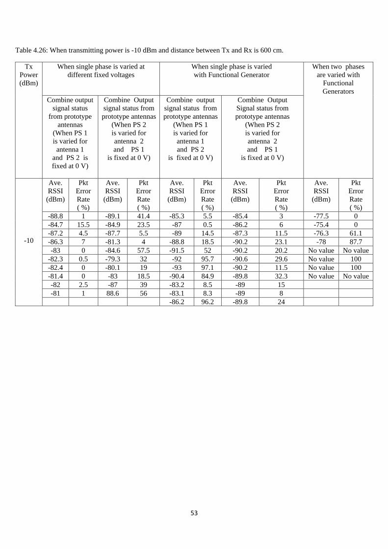
53


Tx Power (dBm)



When two phases are varied with

Functional Generators







is fixed at 0 V)



is fixed at 0 V)



is fixed at 0 V)

-10

Ave. RSSI (dBm)

Pkt Error Rate ( %)

Ave. RSSI (dBm)

Pkt Error Rate ( %)

Ave. RSSI (dBm)

Pkt Error Rate ( %)

Ave. RSSI (dBm)

Pkt Error Rate ( %)

Ave. RSSI (dBm)

Pkt Error Rate ( %)

-88.8 1 -89.1 41.4 -85.3 5.5 -85.4 3 -77.5 0 -84.7 15.5 -84.9 23.5 -87 0.5 -86.2 6 -75.4 0 -87.2 4.5 -87.7 5.5 -89 14.5 -87.3 11.5 -76.3 61.1 -86.3 7 -81.3 4 -88.8 18.5 -90.2 23.1 -78 87.7 -83 0 -84.6 57.5 -91.5 52 -90.2 20.2 No value No value

-82.3 0.5 -79.3 32 -92 95.7 -90.6 29.6 No value 100 -82.4 0 -80.1 19 -93 97.1 -90.2 11.5 No value 100 -81.4 0 -83 18.5 -90.4 84.9 -89.8 32.3 No value No value -82 2.5 -87 39 -83.2 8.5 -89 15 -81 1 88.6 56 -83.1 8.3 -89 8

-86.2 96.2 -89.8 24

54


Tx Power (dBm)




Generators Combine output

signal status from prototype

antennas (When PS 1 is varied for antenna 1




is fixed at 0 V)



is fixed at 0 V)



is fixed at 0 V)

-20

Ave. RSSI (dBm)

Pkt Error Rate ( %)

Ave. RSSI (dBm)

Pkt Error Rate ( %)

Ave. RSSI (dBm)

Pkt Error Rate ( %)

Ave. RSSI (dBm)

Pkt Error Rate ( %)

Ave. RSSI (dBm)

Pkt rror Rate ( %)

-92.1 24 -96.9 70.7 -92.8 92.5 -97.9 75.3 -88.6 3.5 -95.9 31 -96.4 95.7 -93.3 82.9 -95.4 25.5 -88.2 6 -96.9 14 -98 68 -93.5 91.1 -97.6 93.3 -88.2 64.9 -97.2 25 -95.7 28.5 -92.4 65.5 -94 95.5 -90.3 84.5 -96 19 -93.4 16.5 -91.7 51.1 -95.9 91.8 -89 50

-94.7 12.5 -94 23.1 -95 48.1 -94.8 90.5 No value 100 -93 8.5 -94 23.5 -94.6 86.8 -94.7 81.1 No value 100

-94.8 22.4 -93.4 23.1 -94.5 17.1 -95.5 91.4 No value 100 -92 15.5 -94.7 45.2 -96 22.2 -97.9 82.7

-96.2 60.7 -94.6 35 No value No value -98.1 81.1 -96.5 96.7 -97 83.6 No value No value -97.1 71.3

55

Table 4.28: When transmitting power is -10 dBm and Concrete wall barrier between Tx and Rx.

Tx Power (dBm)




Generators







is fixed at 0 V)






is fixed at 0 V)

-10

Ave. RSSI (dBm)

Pkt Error Rate ( %)

Ave. RSSI (dBm)

Pkt Error Rate ( %)

Ave. RSSI (dBm)

Pkt Error Rate ( %)

Ave. RSSI (dBm)

Pkt Error Rate ( %)

Ave. RSSI (dBm)

Pkt Error Rate ( %)

-94.8 30.7 -86.8 17 -87.1 6.5 -88.1 46.5 -88.8 10.5 -89.5 4 -91 13.5 -88 24.5 -86.9 53 -90.9 8.5 -89 1 -90.7 10.5 -88.9 36 -89.4 80.9 -93.6 78.7

-91.2 0.5 93.4 3.5 -88.9 28.5 -89.6 80.5 -96 83.3 -92.9 6 -88.7 12.5 -89 31 -91.1 90.9 No value -95.1 17.6 -85 1 -88.7 32 -89.6 92.5 No value 100 -94.6 12.6 -85.1 8 -89.3 45.5 No value No value No value No value -93 9 -85 5 -90.5 67.2 -91.1 85.4 No value 100 -93 16.5 -85 1 -89.6 39.5 -90.8 97.1

-91.2 14.5 -85.6 4 -87.3 14.5 -91 94.4

56


Tx Power (dBm)



When two phases are varied with Functional Generators







is fixed at 0 V)






is fixed at 0 V)

-14

Ave. RSSI (dBm)

Pkt Error Rate ( %)

Ave. RSSI (dBm)

Pkt Error Rate ( %)

Ave. RSSI (dBm)

Pkt Error Rate ( %)

Ave. RSSI (dBm)

Pkt Error Rate ( %)

Ave. RSSI (dBm)

Pkt Error Rate ( %)

-97.4 29.6 -93.9 17.4 -92.4 62.8 -92.7 39.5 No value 100 -93.6 20.5 -93.2 23 -89.5 40.5 -93.3 17.6 -96.5 97.1 -95.1 8 -94.8 28.9 -91.6 52 -95.4 53.3 No value 100 -98.1 71.5 -96.3 31.8 -91.5 52 -90 14 -98 66.7 -97.5 25.8 -98.4 88 -92.6 63.8 -91.2 84.8 No value No value -96.1 15.5 No value No value -92.8 76.3 -91.1 93 No value No value -97.3 65.9 -98.3 54.8 -92.5 65.5 No value No value No value No value -97.4 16.2 -95.6 36.5 -93.6 73.4 No value No value No value No value -98 24.5 -93.3 22 -91.6 53.6 No value No value

-95.5 28.1 -93.6 22.5 -92.5 59.4 -91 80 -94.8 84 No value No value -93.2 75.1 No value No value

57


Tx Power (dBm)



When two phases are varied with Functional Generators






is fixed at 0 V)







is fixed at 0 V)

-18

Ave. RSSI (dBm)

Pkt Error Rate ( %)

Ave. RSSI (dBm)

Pkt Error Rate ( %)

Ave. RSSI (dBm)

Pkt Error Rate ( %)

Ave. RSSI (dBm)

Pkt Error Rate ( %)

Ave. RSSI (dBm)

Pkt Error Rate ( %)

-99 94.6 No value No value -94.9 59.2 -94.1 22 -98 88.9 -98.4 62 -98.7 58 -95.7 67 93.1 16.5 -98 93.3 -96.1 12 -96.4 15 -94.5 65.3 -92.7 14 No value 100 -98.7 61.6 -98.1 33.7 -94.9 76.1 -93.2 21 No value 100 -98 59.6 -98.8 95.2 -96.8 85.3 -92.9 77.3 No value No value

-98.2 61 -99 86.5 -95.5 85.6 -92.7 88.6 No value No value -98.9 66.7 No value No value -95.7 84.1 -94 94.7 No value No value -98.7 72.7 No value No value -95.6 83.4 No value No value No value 100 -97.1 21.2 -98.9 61.4 -95.9 58.6 No value No value -97.9 25.5 No value No value -94 66 No value No value

-95.6 63 No value No value -98.2 85.1 No value No value

After analysis the above comparison tables for different power levels and distances in both LOS and close environment, it is clear that sweeping one of the phase shifters makes link quality worse comparative to fixed control voltage based measurements but sweeping both phase shifter provides better results between all measurement configurations concerning certain frequency of interests.

58

6 Conclusion and future work

6.1 Conclusion

In this thesis work, mainly focus on antenna diversity systems with opportunistic combining to improve the signal reliability through reducing fading. Placing two PIFA in different dimensions of PCB is designed and simulated in HFSS. In the HFSS simulation results, the correlation coefficients by S-parameters and radiation patterns are not the same, it is because the unknown losses in the materials or other reasons. Wilkinson combiner is designed and simulated in ADS and Phase shifter is used to changes the phase of input signal with the help of controlling voltage and Rogers 4350B substrate is used for PCB fabrication and prototypes were made in PCB lab.

Measurements have been done in both reverberation chamber and office environments. In office environment experiment with ZigBee board, sweeping both phases gives good results comparatively with fixed and sweeping single phase for certain frequencies and in reverberation chamber, it does not show so good result in comparison with monopole antenna but sometimes it shows some small improvement with opportunistic diversity, and sometimes the performance was the same as with just one monopole.

6.2 Future work

Uncorrelated between antenna branches is an important issue for signal improvement which depends on correlation coefficients, lower the correlation coefficients, the higher the signal reliability in multipath propagation. So, to improve antenna diversity design to make the correlation coefficients be close to zero. Diversity technique was not tested in a good way in the RC with absorbers due to presence of few waves which mean the signal environment was sparse. One way to move forward would be tested in a Rayleigh environment that is not highly resonant. Such equipment could be the so-called multipath propagation simulator (MPS). The same above measurements could verify with without antennas prototype through connecting two separate alone antenna with extra cable. Bluetooth device (incoherent FSK) can also be used instead of ZigBee board for measurement purpose.

59

7 References

[1] Lars Ahlin, Jens Zander, Ben Slimane and Studentlitteratur “Principles of Wireless Communications” ISBNμ λ1-44-03080-0, 2006.

[2] Magnus Jobs, Mathias Gruden, Paul Hallbjörner, Anders Ryberg ‘Antenna Diversity with Opportunistic Combining for ASK System With Single Channel Receivers’.

[3] David M.Pozar ‘ Microwave Engineering- third edition’, ISBNμλ78-81-265-1049-8, John Wiley & Sons(Asia) Pte. Ltd., Singapore,1989.

[4] Vicent F.Fusco, ’Foundation of Antenna Theory and Techniques’, ISBNμλ78-81-317-1125-5, Person Education, Ltd, 2005.

[5] Pozar, David M ‘Microwave and RF design of wireless system’. ISBNμ 0-471-32282-2, John Wiley & Sons, Inc, 2001.

[6] http://en.wikipedia.org/w/index.php?title=File:Sidelobes_en.svg&page=1, [acesssed 16/10/2012].

[7] Reinhold Ludwig, Gene Bogdanov, ‘ RF Circuit Design Theory and Applications’, ISBN-13:978-01-314-7137-5, Person Education, Inc, Upper Saddle River, NJ 07458.

[8] Pail Hallbjörner, β005,’The Significant of Radiation Efficiencies When Using S-Parameters to Calculate the Received Signal Correlation From Two Antennas’, IEEE Antenna and Wireless Propagation Letters, Vol.4, pp.97-99.

[9] www.antenna-theory.com/antennas/patches/pifa.php, [accessed 18/10/2012].

[10] Kyohei Fujimoto ’Mobile Antenna System Handbook - Third edition’ ISBN-13:978-1-59693-126-8, ARTECH HOUSE, INC. 685 Canton Street Norwood, MA 02062.

[11] Vanja Plicanic, May 2004,’ Antenna Diversity Studies and Evalution’, Master of Science Thesis, in cooperation with Ericsson Mobile Communication AB, Department of Electroscience, Lund University.

[12] http://www.qsl.net/v/va3iul/Phase_Shifters/Phase_Shifters.pdf, [accessed 18/10/2012].

[13] http://www.microwaves101.com/encyclopedia/phaseshifters.cfm, [accessed 18/10/2012].

[14] Joakim Östh “Opportunistic combining calculation” presented on presentation at Linköping University, Sweden, 2012-10-11.

[15] http://www.hittite.com/content/documents/data_sheet/hmc928lp5.pdf, [accessed 18/10/2012].

[16] http://www.antenova.com/Product%20Specs/FE010315-N-Product-Specification-Mica.pdf, [accessed 18/10/2012].

antenna diversity with opportunistic combining

Documents