Anti-smoking policies and smoker well-being: evidence from Britain

IFS Working Paper W13/13

Andrew Leicester Peter Levell

Anti-smoking Policies and Smoker Well-Being: Evidence From

Britain∗

Andrew Leicester†and Peter Levell‡

June 14, 2013

Abstract

Anti-smoking policies can in theory make smokers better o�, by helping smokers with time-inconsistent

preferences commit to giving up or reducing the amount they smoke. We use almost 20 years of British

individual-level panel data to explore the impact on self-reported psychological well-being of two policy

interventions: large real-terms increases in tobacco excise taxes and bans on smoking in public places.

We use a di�erence-in-di�erences approach to compare the e�ects on well-being for smokers and non-

smokers. Smoking behaviour is likely to be in�uenced by policy interventions, leading to a selection

problem if outcomes are compared across current smokers and non-smokers. We consider di�erent ways

of grouping individuals into `treatment'and `control' groups based on demographic characteristics and

observed smoking histories. We �nd fairly robust evidence that increases in tobacco taxes raise the

relative well-being of likely smokers. Exploiting regional variation in the timing of the smoking ban

across British regions, we also �nd some evidence that it raised smoker well-being, though the e�ect is

not robust to the measure of well-being. The economic signi�cance of the e�ects also appears to be quite

modest. Our �ndings therefore give cautious support to the view that such interventions are at least

partly justi�able because of the bene�ts they have for smokers themselves.

JEL: D03, D12, H23, H31

Keywords: Smoking, taxation, happiness, well-being, time inconsistency, commitment

∗Address for correspondence: a.leicester@ifs.org.uk. This research was funded by the Nu�eld Foundation (referenceOPD/39073), and the ESRC Centre for Microeconomic Analysis of Public Policy (CPP, reference RES-544-28-5001) at IFS.Data from the British Household Panel Survey are produced by University of Essex Institute for Economic and Social Research.The data are Crown Copyright and reproduced with the permission of the Controller of HMSO and the Queen's Printer forScotland. The authors would like to thank Ian Crawford of IFS and Oxford, Tom Crossley of IFS and Essex, Deborah Arnottand Martin Dockrell of Action on Smoking and Health, Howard Reed of Landman Economics and Robert West of UCL forcomments on earlier drafts and useful discussions. They would also like to thank seminar participants at the Institute for FiscalStudies and the Royal Economics Society annual conference for helpful advice. Views expressed are those of the authors andnot the Institute for Fiscal Studies. Any errors are our own.†Institute for Fiscal Studies‡Institute for Fiscal Studies and University College London

1

1 Introduction

It has long been recognised that policies to reduce smoking behaviour can be justi�ed by the negative

externalities associated with smoking.1 Costs including passive smoking and the net cost to public healthcare

are borne by wider society but not the smoker, leading to excessively high levels of smoking from a socially

optimal perspective. Policies such as tobacco excise taxes which raise the cost of smoking can therefore

improve overall social welfare, though are usually assumed to make smokers individually worse o�. However,

recent insights from behavioural economics suggest that smokers themselves may bene�t from anti-smoking

interventions. In particular, when smokers are time inconsistent, they may not be acting in their own best

interests in making their smoking decisions. They make plans to give up smoking in the future but are unable

to act on them when the future comes and they are faced with the immediate decision to smoke again.2 In

such cases, anti-smoking policies could help smokers commit to giving up, meaning the policies could be

further rationalised by the commitment bene�ts they confer on smokers.

It is hard to determine straightforwardly whether or not there is such a rationale for intervention. Empir-

ical predictions about how smoking behaviour responds to price increases (now or expected in the future), for

example, are the same whether or not smokers are assumed to be time inconsistent. A small emerging litera-

ture, beginning with Gruber and Mullainathan (2005), has started to look at how the self-reported well-being

of smokers responds to policy reforms. Assuming that self-reported well-being is informative about individual

welfare, evidence that smokers are made relatively better-o� when anti-smoking reforms are enacted would

be suggestive of time inconsistency. The key methodological challenge of this literature is to overcome the

fact that smoking behaviour is in itself partly determined by policy reforms.

This paper contributes to this emerging literature in a number of ways. Most signi�cantly, we make

use of a long individual-level panel dataset which includes information on smoking behaviour alongside self-

reported well-being. Previous studies looking into the same question have made use of cross-sectional data,

relying on a modelled propensity to smoke (assumed exogenous to policy changes) to identify the impact

on well-being. Using panel data allows us to make use of individuals' own smoking histories to construct

treatment groups of people likely to bene�t from the commitment value of anti-smoking policies, but where

treatment status is not itself determined by policy changes. We also explore the di�erential impact of the

policies across education groups. If low education (a proxy for low lifetime income) people are more prone to

time-inconsistency, they may see greater welfare bene�ts from anti-smoking policies. This has implications

for the distributional e�ects of such policies.

We look at the e�ect both of tobacco excise taxes and bans on smoking in public places. Bans have

1A summary of the evidence on the magnitude of smoking-related externalities is in Crawford et al. (2010).2Around two thirds of adult smokers in England say they would like to give up (NHS Information Centre, 2012).

2

been implemented in a number of OECD countries in recent years, as anti-smoking policies move beyond

price-based incentives toward more direct regulation of smoker behaviour. We exploit time-speci�c variation

in cigarette taxation and regional variation in when smoking bans were implemented to identify the impact

of these measures on smoker well-being. Our study provides the �rst evidence on this issue for Britain, which

has been active both in implementing bans on smoking and in raising tobacco taxes. As at July 2011, British

excise taxes on cigarettes were the second-highest (behind Ireland) in the EU.

To preview brie�y our key results: we �nd evidence that higher real tobacco taxes increase the relative

well-being of likely smokers, suggestive of time inconsistency in smoker behaviour. This result is broadly

robust to di�erent de�nitions of treatment groups and measures of well-being. We �nd similar evidence that

bans on smoking in public places raise smoker well-being, though this result is more sensitive to the measure

of well-being. We do not �nd any di�erential e�ects across education groups.

The rest of the paper proceeds as follows. Section 2 recaps the recent evolution of UK tobacco taxes and

bans on smoking in public places, our main policies of interest. Section 3 then describes the main economic

and conceptual ideas around smoker behaviour and the implications of anti-smoking policies for smoker

welfare. Section 4 develops the empirical strategy and describes the data used for the analysis. Section 5

describes the main results, and Section 6 concludes.

2 Policy background

2.1 Smoking taxation

Excise taxes have long formed an important part of government policy to limit tobacco consumption.

Cigarette taxation in the UK includes both a speci�c component (¿3.35 per pack of 20 cigarettes in 2012)

and an ad-valorem component (16.5% of the tax-inclusive price).3 Tobacco taxes are forecast to raise around

¿9.8 billion in �nancial year 2012/13, 1.7% of total receipts.

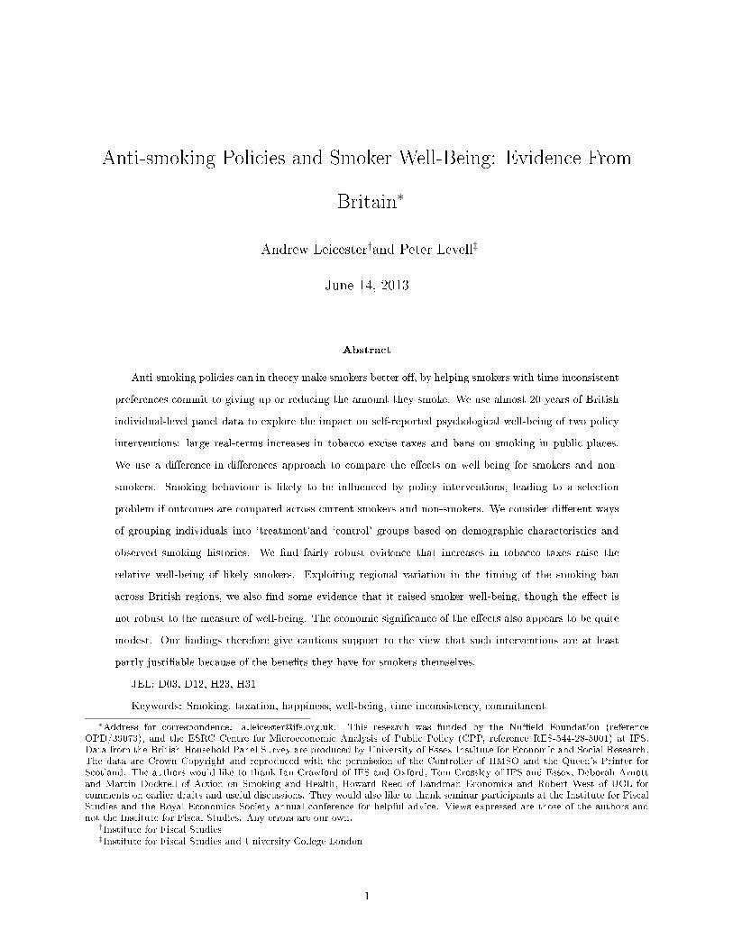
Figure 1 shows real-terms excise taxes on cigarettes in the UK between 1988 and 2012, based on data from

HM Revenue and Customs (HMRC, 2012). We convert the speci�c and ad valorem components into a single

rate per pack of 20 cigarettes using information on cigarette prices from the O�ce for National Statistics to

place a cash value on the ad-valorem component.4 This is then converted to real June 2012 values using the

all-items Retail Prices Index (RPI).

3Other tobacco products generally face speci�c taxes by weight. Rates can be found athttp://www.hmrc.gov.uk/rates/tobacco-duty.htm.

4Series CZMP at http://www.ons.gov.uk/ons/datasets-and-tables/data-selector.html?table-id=3.1&dataset=mm23.

3

Figure 1: Real-terms cigarette excise tax per pack of 20, 1988�2012

0

50

100

150

200

250

300

350

400

450

500

19

88

19

89

19

90

19

91

19

92

19

93

19

94

19

95

19

96

19

97

19

98

19

99

20

00

20

01

20

02

20

03

20

04

20

05

20

06

20

07

20

08

20

09

20

10

20

11

20

12

Rea

l exc

ise

tax

(pen

ce p

er p

ack,

Ju

ne

20

12

pri

ces)

Source: ONS data on prices (series CZMP, Consumer Price Indices). UKtradeinfo data on taxes

(www.uktradeinfo.com). Converted to June 2012 prices using the all-items Retail Prices Index.

Real tax rates more than doubled over the period. Between 1993 and 2000, there was an explicit `escalator'

policy to increase the speci�c tax in real terms, by 3% above in�ation at �rst and then, from July 1997, by

5%. Over this period, real tobacco taxes increased by around 64% from ¿2.32 to ¿3.81 per pack. Beginning

with the 2001 Budget, tobacco taxes were then frozen in real terms. In December 2008, tax rates increased

to `o�set' a temporary reduction in the rate of Value Added Tax (VAT) from 17.5% to 15% enacted as a

�scal stimulus (though note this was not reversed when VAT rates rose again in January 2010). Real taxes

then rose by 1% in 2010, 2% in 2011 and 5% in 2012.

A large empirical literature suggests that prices are an e�ective instrument to reduce smoking rates. A

meta-study by Gallet and List (2003) found an average price elasticity of demand for cigarettes of around

-0.4 to -0.5. Chaloupka and Warner (2000) �nd that price increases reduce demand both along the extensive

and intensive margins (i.e. the propensity to smoke at all and how much is smoked conditional on smoking

anything), and that increases in tobacco taxes tend to be passed through more than one-for-one into �nal retail

prices. A number of papers have highlighted other behavioural responses to price rises, such as substitution

to higher tar and nicotine cigarettes and smoking more intensively (Evans and Farrelly, 1998; Farrelly et al.,

4

2004; Adda and Cornaglia, 2006) which could partially or wholly o�set the impact of reduced smoking on the

intensive margin. Smokers could also substitute by trading down to cheaper brands or forms of tobacco, such

as hand-rolling tobacco (HRT) rather than pre-rolled cigarettes. There is evidence of a switch towards HRT

in the England. Data from the NHS Information Centre (2012) suggest that in 1990, around 91% of adult

smokers smoked mostly pre-rolled cigarettes whilst 10% smoked hand-rolled. By 2010, the proportions were

69% and 31%. Note, though, that the taxation of HRT and cigarettes have moved in very similar ways over

time (HMRC, 2011a). Further, given the overall decline in smoking rates, the prevalence of HRT smokers

amongst all adults rose only from 3% to 6% whilst the proportion of cigarette smokers fell from 26% to 14%.

Smokers may also respond by purchasing illicit tobacco (e.g. from low-tax jurisdictions by people living

near borders, or through increased organised smuggling). Stehr (2005) uses US data and �nds cigarette

purchases repond more than cigarette consumption to tax changes, ascribing much of the di�erence to evasion.

Price is not the only determinant of evasion, which will also depend on resources devoted to enforcement.

Estimates for the UK (HMRC, 2011b) suggest that the illicit market share for cigarettes fell from 21% in

2000/01 to 10% in 2009/10 (from 61% to 46% for HRT over the same period) following a policy strategy to

reduce smuggling including greater enforcement at borders and punishments for those caught (HMCE and

HMT, 2000). We discuss the possible implications for our analysis in Section 5.

2.2 Bans on smoking in public places

Over the last decade or so a number of countries have implemented bans on smoking in public places. In the

UK, a ban was �rst introduced in Scotland from 26 March 2006, followed by Wales (2 April 2007), Northern

Ireland (30 April 2007) and �nally England (1 July 2007). de Bartolome and Irvine (2010) develop a model in

which bans raise the cost of smoking by limiting the ability of smokers to take in a smooth stream of nicotine

throughout the day. Bans can also raise the hassle costs of smoking. A review by Hopkins et al. (2010) �nds

a small but consistent e�ect of `smokefree' policies including bans to reduce smoking at the extensive and

intensive margin. By contrast, a number of recent studies (Adda and Cornaglia, 2010; Carpenter et al., 2011;

Anger et al., 2011; Jones et al., 2011) have used quasi-experimental approaches exploiting regional variation

in the timing of bans and found no signi�cant e�ect on overall smoking prevalence or intensity, though

some evidence of heterogeneous responses amongs particular groups (e.g. those most likely to frequent bars

and restaurants or heavy smokers). Shetty et al. (2009) �nd no impact of smoking bans in workplaces on

hospitalisation rates or mortality from heart attacks, comparing areas where bans were introduced to control

areas where they were not. These results suggest bans tend to displace where people smoke. Adda and

Cornaglia (2010) draw on time use data to suggest that following bans, smokers spent more time at home.

5

They argue that bans may have increased children's exposure to second-hand smoke as a result, though

the �ndings have been disputed by Carpenter et al. (2011) drawing on self-reported records of exposure by

non-smokers.

3 Economic models of smoker behaviour and welfare implications

of policy interventions

The workhorse economic model of smoking has been the `rational addiction' framework (Becker and Murphy,

1988). Consumption of an addictive good like tobacco builds up a `stock' of addiction. Utility in each period

depends not only on current consumpion of tobacco and other goods, but also the accumulated addiction stock

(re�ecting for example the health costs of smoking). This introduces a non-separability in preferences across

periods, such that current smoking will be in�uenced by expectations of future tobacco prices. Addiction is

characterised by `adjacent complementarity': the higher the addiction stock, the higher the marginal utility

from smoking. Consumers pick a path for current and future consumption of tobacco and the non-addictive

good, taking into account how current decisions a�ect future utility. In the absence of any unexpected shocks,

they will follow through that plan. A key implication of the rational addiction framework is that increases of

the cost of smoking (such as higher tobacco taxes or public smoking bans) will reduce smokers' well-being.

The rational addiction model has been extended in a number of ways to account for smokers expressing

regret about their smoking behaviour or failing to give up when they express a preference to do so, whilst

maintaining the basic assumption that smoking decisions are the result of utility maximising behaviour.

For example, if consumers make boundedly rational decisions with informational uncertainty about their

tendency to become addicted (Orphanides and Zervos, 1995), then taking up smoking might look optimal

given some perceived risk of addiction which later turns out to be wrong, but continued smoking is then

optimal given the addiction stock which has been built up. There is some empirical evidence that young

people in particular make smoking choices without full information on the risk of addiction (Gruber and

Zinman, 2001; Loewenstein et al., 2003; Schoenbaum, 2005).5 Suranovic et al. (1999) build in an adjustment

cost of reducing smoking (perhaps re�ecting the pain of withdrawal) which may not be fully anticipated by

people making smoking decisions. Jehiel and Lilico (2010) argue that consumption decisions may be taken

with limited foresight: consumers may make smoking choices only considering some proportion of the future

rather than the whole lifetime. In this framework it is possible that the lifetime optimal choice would be

not to smoke but the limited foresight optimal choice is to smoke. They show that if the foresight horizon

5It is also possible that people may misperceive the health risks of smoking which would cause them to come to regret theirdecisions as and when their information changed. Sloan and Platt (2011), though, suggest that if anything young people tendto overestimate the risk of health harms from smoking.

6

increases with age (perhaps re�ecting increased learning or maturity), older people will give up or, in some

cases, cycle between smoking and not smoking.

Whilst these ideas suggest why people come to regret past decisions or change their behaviour in the light

of new information or experience, they do not clearly explain why people say they plan to give up but fail

to do so.6 Another development of the theory has considered that people su�er from a time inconsistency

problem. The rational addiction framework assumes that there is a constant discount rate: from today's

perspective, utility in two periods is discounted twice as much as utility next period. If, instead, people

discount the immediate future more heavily relative to the far-distant future, then it is possible that a plan

to quit looks optimal from today's perspective but is no longer optimal when the time comes to follow that

plan through. As a result, the passage of time alone is enough to change behaviour, hence the expression `time

inconsistency'. A key implication of time inconsistency is that consumers place positive value on mechanisms

which allow them to commit to a particular plan of action. Bryan et al. (2010) provide evidence on the

demand for commitment devices in a number of contexts. Frederick et al. (2002) and DellaVigna (2009)

survey evidence for time-inconsistency in lab and �eld experiments respectively.

The hyperbolic discounting model of Laibson (1997) builds this change in discount factors into standard

models of people making inter-temporal choices. O'Donoghue and Rabin (1999) look at this in the context

of procrastination over whether or not to carry out a discrete action such as giving up smoking. Gruber and

K®szegi (2000, 2001, 2004) build hyperbolic discounting into the rational addiction framework to think about

continuous choices over cigarette consumption. Their model forms the basis for our empirical approach - we

outline the main points below but full details of the derivation and proofs can be found in their papers.

Consumers allocate income across two goods in each period t, addictive tobacco at and a non-addictive

consumption good ct. Utility is assumed to be additively separable in the two goods. Consuming the addictive

good builds up an addiction stock St which depreciates at a constant rate 0 < d < 1 in each period. Utility

from consuming the addictive good depends on the accumulated stock as well as the current consumption.

Thus the utility function takes the form:

Ut = v(at, St) + u(ct)

St+1 = (1− d)(St + at)

Addiction in this model arises when vaS > 0, that is, the marginal utility of current tobacco consumption

increases in the addiction stock. The harmful health consequences of tobacco can be modelled by assuming6Assuming of couse that a stated preference to give up is genuine and does not re�ect a bias of survey respondents to give

`socially acceptable' answers.

7

vS < 0 .

Under quadratic utility, the subutility functions can be written as:

v(at, St) = αaat + αSSt + αaSatSt +αaa

2a2t +

αSS

2S2t

u(ct) = αcct

with αa, αc, αaS > 0 and αaa, αSS , αS < 0. Tobacco is sold at a price p in each period, and the non-addictive

good is sold at a normalised price of 1. Consumption of the non addictive good is therefore given as residual

income, ct = It − pat.

Consumers maximise discounted current and future utility. Utility over T periods is given as:

U = Ut + β

T−t∑i=1

δiUt+i

with β, δ ∈ (0, 1). Hyperbolic discounting in this model arises because from the period t perspective, utility

in the next period t + 1 is discounted by βδ whereas utility between periods t + 1 and t + 2 (or any two

future consecutive periods) is discounted only by δ. In other words, the immediate future is more heavily

discounted than the distant future. In the next period, the discount rate between t + 1 and t + 2 will then

change to βδ.

Consumers are assumed to be aware that their discount rates are time-varying in this way. It is also

assumed that from a welfare perspective, what matters for consumers are their long-run preferences (i.e.

ignoring the additional immediate discount factor β).7 The question is then how an increase in the price of

tobacco a�ects consumer welfare. Since (conditional on income) utility will depend on the price of tobacco

and the addiction stock in this model, from today's perspective, the expression of interest is:

d

dpU1(S1, p) =

d

dp[v(a1, S1) + αc(I1 − pa1) + δU2(S2, p)]

Gruber and K®szegi (2004) show using an iterative procedure that the derivative of discounted utility with

respect to the price of tobacco is given by:

−αc

T∑j=1

δj−1aj

− (1− β)T∑

j=1

δj−1 ∂aj∂p

va(aj , Sj)− pαc

β

7This is of course something of a controversial assumption: it may be thought that at least some weight should be given tothe short-term preference as well. For a discussion see Bernheim and Rangel (2005).

8

The �rst term is the standard result where there is no time inconsistency: higher tobacco prices reduce

utility by increasing the cost of smoking. The second term is the commitment bene�t of higher prices. In

each period, consumers smoke by more than they would `like' on the basis of their long-term preferences

because the immediate future is more heavily discounted. Higher prices induce a consumption response

∂aj

∂p < 0 which helps time-inconsistent consumers to act more in line with their long-run preferences. The

whole second expression is positive: that is, the utility cost of higher prices is mitigated by the self control

bene�t.

To reiterate: the important implication of building time inconsistency into the addiction framework is

that increases in the cost of addictive goods (such as tobacco) need not reduce individual welfare. With

time inconsistency, higher costs provide a `commitment' bene�t to smokers, reducing future consumption

towards levels that would be optimal in a time consistent model.8 Gruber and K®szegi (2004) carry out

a calibration exercise to show that higher prices are particularly likely to be welfare-improving when the

hyperbolic discount factor is low (that is, when people are very impatient over the immediate future). This

suggests that increases in tobacco tax rates can make smokers better o�, giving a rationale for smoking taxes

even without negative externalities. A similar argument can be made for other policies which raise the cost

of smoking, such as bans on smoking in public places.

If we can interpret measures of self-reported well-being in surveys as a measure of individual welfare (or at

least assume that they are positively correlated with welfare), then this model implies that when smokers are

very time-inconsistent their reported well-being will rise when smoking costs increase, whereas non-smokers

will be una�ected.9 This forms the basis of our empirical strategy outlined in the next section.

8As noted in Gruber and Mullainathan (2005), other `behavioural' models besides time inconsistency can generate a demandfor commitment. Bernheim and Rangel (2004) discuss `cue-based' consumption models, where consumption decisions dependon particular environmental signals (such as intending not to smoke but being in�uenced to do so when in the company of othersmokers). Smokers who are aware of this would demand mechanisms that help them avoid those cues. The model of Gul andPesendorfer (2001, 2007) considers the `self-control' costs that people face to avoid `temptation' - think of the willpower e�ortneeded not to smoke when cigarettes are easily available - and so demand mechanisms that reduce self-control costs. In bothcases, simple versions of these models imply that higher prices make smokers worse-o� because consumption in the presence ofa cue or the temptation value placed on smoking is essentially unresponsive to price. However, allowing cue-based demand ortemptation utility to vary with price can restore the interpretation that smoker welfare improves when the costs of smoking rise.

9Larsen and Fredrickson (1999) and Stutzer and Frey (2010) summarise evidence on the relationship between survey-basedmeasures of happiness and other indicators of well-being (including observer-reports of happiness and economic indicators).There are of course reasons why non-smokers may be impacted by higher tobacco taxes as well. Reduced smoking rates mayhave positive bene�ts for non-smokers in the presence of negative externalities, for example. The use of increased tobacco taxrevenues to fund public spending or reduce other taxes may also bene�t non-smokers. However it might be expected that thesegains are second-order in magnitude relative to the direct gains for time-inconsistent smokers.

9

4 Empirical methods

4.1 Empirical strategy

We carry out a reduced-form analysis of the impact of anti-smoking policy interventions (increases in cigarette

excise taxes and bans on smoking in public places) on self-reported individual measures of well-being. In

particular, we compare whether these policies have a di�erential impact on the well-being of the people most

likely to bene�t from the commitment value they generate: smokers or groups of people who, on the basis

of their observable characteristics or past smoking behaviour, are likely smokers. We exploit time-varying

real excise taxes and time- and location-varying bans on smoking alongside detailed long-term panel data

reporting happiness and smoking measures for a large sample of British adults to conduct our analysis. The

data are described in more detail in Section 4.2.

We draw on a number of recent studies, most notably the pioneering work of Gruber and Mullainathan

(2005). Using US and Canadian data, they �nd evidence that higher real cigarette excise taxes signi�cantly

reduce the tendency of likely smokers to report being unhappy relative to those unlikely to smoke. Their

results for the US imply that an excise tax of $1.60 has the same e�ect on the happiness of likely smokers

as moving from the poorest income quartile to the next poorest quartile. More recently, mixed evidence has

emerged on the e�ect of smoking bans on the relative well-being of smokers. Odermatt and Stutzer (2012) �nd

a negative e�ect, exploiting variation in the timing of bans across European countries and regions. However,

Brodeur (2013) uses county-level data from the US and �nds a positive e�ect.

Other studies have provided empirical support that smokers support anti-smoking policies. Hersch (2005)

uses US data to look at support for restrictions on smoking in six di�erent types of public place among

current smokers, distinguishing those who say they want to quit (who may therefore reveal themselves to be

su�ering from time inconsistency) from those who do not. The results show stronger support for the bans

amongst those who want to give up. Interestingly, the support is even stronger for those who have tried

and failed to quit than those who are planning to try for the �rst time. They suggest this is evidence that

those who have failed before have higher quit costs (such as the pain of withdrawal or di�culty in obtaining

support for giving up elsewhere) and so would place even greater value on the policies. Kan (2007) �nds

evidence in Taiwanese data that smokers who want to quit express more support for higher tobacco taxes

and smoking bans in public places or at work. Badillo Amador and López Nicolás (2011) �nd similar results

in Spanish data.

10

4.1.1 Cigarette excise taxes

In looking at the impact of tobacco excise taxes, we compare how they a�ect the self-reported well-being of

likely smokers relative to non-smokers. The basic estimating equation takes the form:

Hit = α+ βt + γTt + δSit + ξ (Tt × Sit) + θXit + εit

where Hit is a measure of well-being (i indexing individuals and t indexing the time (year and month) in

which the individual is observed), Tt is the in�ation-adjusted tobacco tax rate, Sit is a variable indicating

smoker status and Xit is a vector of individual-speci�c observable characteristics that could a�ect well-being.

We detail the set of covariates in Section 4.2. Because we use panel data, we cluster the standard errors at

the individual level to account for any correlation in the error structure within individuals over time. The

parameter of interest is ξ which measures the di�erential impact of real excise taxes on the well-being of

smokers relative to non-smokers. A positive coe�cient would be suggestive of the commitment bene�ts from

higher taxation seen in time inconsistency models of smoker behaviour.

Simply using current smoker status as the measure of Sit in the model may lead to problems since smoking

behaviour today will be endogenous to current tax rates. This leads to a selection e�ect: if those who continue

to smoke following a tax rise have lower happiness than those who quit, this will bias downward the coe�cient

ξ.

We consider a number of approaches to deal with this. The �rst closely follows that of Gruber and

Mullainathan (2005). In place of current smoking status, they use a modelled estimate of an individual's

propensity to smoke based on observable characteristics, where smoking propensity is not a function of current

smoking tax rates. Using the �rst wave of data (from 1991) we estimate a probit model of the propensity

to smoke where the dependent variable is a dummy variable for current smoker status and the independent

variables are the same covariates used in the happiness equation.10 We use the parameter estimates to predict

the likelihood that individuals observed in each year would have been smokers had they been observed with

those covariates in the 1991 sample. This propensity P 91it is then used in place of Sit in the well-being

equation.11 There are two small di�erences between the Gruber and Mullainathan (2005) approach and our

10The model results from this probit are detailed in the Appendix. Controlling for other observables, women are less likelyto smoke than men. People in poorer households and with lower educational attainment are more likely to smoke, as are thosewho are unemployed. Divorced, widowed or co-habiting people are more likely to smoke than married people. Private and socialrenters are more likely to smoke than other tenure types. Those with breathing problems are more likely to be smokers.

11Note that as discussed in Gruber and Mullainathan (2005), we do not use P 91it as an instrument forSit; rather, it directly

replaces it as the object of interest in the estimating equation. Further, as we use the same covariates in the happiness equationand the �rst stage probit equation, identi�cation of the θ parameter in the happiness equation is rather tenuous, driven largelyby the fact that the propensity score is modelled non-linearly whereas the parameters enter linearly into the happiness equation.However, these covariates in the happiness equation are not really of direct interest and serve merely as controls: the keyparameter of interest is ξ which is identi�ed by the interaction of smoking propensity with real tax rates.

11

�rst method. First, we model the propensity only using the �rst year of data rather than estimating separate

propensity models for each year of data. The idea is that modelled propensity to have been a smoker in 1991

is exogenous to tax rates in later years. Second, we account for the fact that we use a two-step method and

use bootstrapping techniques to calculate standard errors in the happiness equation. Not doing this gives

misleadingly small standard errors which could give rise to spurious signi�cance of the key terms of interest.

The fact we are using a long panel dataset of individual smoking and happiness data allows us to consider

two further approaches. Rather than modelling the likelihood that individuals are smokers, we are able to

draw on each individual's own smoking history to assign them to a `treatment' group who would bene�t

from the commitment value of higher taxation under time inconsistency and `control' group who would not.

First, we de�ne those who are smokers in the initial 1991 wave of data as treated and track how their well-

being responds to changes in cigarette excise taxes relative to those who were not smokers in 1991. Second,

we de�ne those who are ever observed to smoke over the entire data period (1991 to 2008) as treated and

those who never smoke as controls. Clearly, those who smoked in 1991 are a subset of those who are ever

observed to smoke over the whole period. It may be that some of those who were not smoking in 1991 but

later took it up were also at risk of starting in earlier years and so would also have valued the commitment

bene�t of taxation. Rather than estimating a propensity weight, these approaches essentially boil down to a

straightforward di�erence-in-di�erences model where treatment status is exogenous to policy reforms.12

One particular implication of the economic model is that likely smokers who exhibit a greater degree of

time inconsistency will see the largest welfare gains from increased taxes, since they will value the commitment

mechanism more highly. There is relatively little evidence on whether time inconsistency varies directly with

observable individual characteristics. Paserman (2008) �nds unemployed workers previously on low incomes

exhibit more time inconsistency than those previously on high incomes. Choi et al. (2011) �nd evidence that

better-o� consumers make decisions consistent with economic rationality, but do not test time-consistency

directly. We investigate the issue by exploring whether there is any di�erential in the relative impact of

taxes on self-reported happiness for smokers in di�erent education groups, where education is assumed to

re�ect di�erences in permanent income across households. This involves further interacting the policy and

smoker status interaction with an educational attainment dummy for those who achieved post-compulsory

quali�cations. Finding larger e�ects for low education individuals could be suggestive evidence that time

12We considered other approaches to determining treatment status. For example, in 1999 individuals were asked about theirsmoking histories over their whole life and we could have classi�ed anyone who had ever smoked as treated. However, aroundtwo-thirds of people had smoked at some point, and we found little di�erence between modelled smoking propensity acrosstreatment and control individuals using this de�nition. It was also unclear that experimental youth smoking would be a gooddeterminant of whether or not people su�ered from time inconsistency problems as a later adult non-smoker. We also couldhave used any past smoking behaviour as a current treatment indicator, such as smoker status in the previous year, rather thansmoker status in the �rst wave. However, the assumption that smoking status a year ago is exogenous to current policy changesis perhaps less credible than assuming exogeneity of initial smoker status to current policy, particularly where people may havehad reasonable expectations about how policy would change in the near future either during the tobacco tax escalator or aroundthe time that smoking bans were being introduced in di�erent regions.

12

inconsistency problems are larger for poorer people.

4.1.2 Bans on smoking in public places

We adopt a similar approach to assessing the well-being e�ect of the ban on smoking in public places.

We exploit regional variation in the timing of the smoking ban. We restrict our sample to those who are

de�ned as likely smokers, and compare changes in smoker well-being for those living in Scotland to those

living in England and Wales in the period following the ban being implemented in Scotland. Again this is

a straightforward di�erence-in-di�erences estimation where the sample is restricted to individuals likely to

bene�t from the commitment value of the ban, and `treatment' is now de�ned across regions rather than

people.

We de�ne groups of likely smokers using individual observed smoking histories in a similar way as described

above.13 First we take smoking status in the �rst year in which individuals are observed. In the analysis

of the smoking ban, we begin in 1999 (rather than in 1991 as for the tax analysis) in order to make use

of regional booster samples in the data which signi�cantly increase the Scottish sample size. Second we

take smoking status over the whole data period beginning from 1999 and de�ne likely smokers as those who

smoked at any time. As above, treatment status should be exogneous to the policy reforms.

The estimating equation is of the form:

Hit = α+ βSCOTit + γPOSTit + ξ (SCOTit × POSTit) + θXit + εit

where SCOTitis a dummy variable for individuals living in Scotland, and POSTitis a dummy for someone

observed in March 2006 or later, following the ban being introduced in Scotland. The coe�cient on the

interaction term ξ then represents the relative impact on well-being for a `smoker' living in Scotland following

the ban there compared to one living in England or Wales before the ban was extended to the rest of Britain.

4.2 Data

Our data come from the �rst eighteen waves of the British Household Panel Survey (BHPS), which covers

the period September 1991 to April 2009. The BHPS is annual survey that initially sampled around 5,500

households (10,000 individuals) in 1991. The survey attempts to follow the same individuals and their natural

descendents through successive waves, even if they move home. All adult members (age 16+) of the sample

households are interviewed each year, including adults that move into the household after the start of the

13Note that we do not use a propensity score approach in this part of the analysis. We could model smoking likelihood andtake some arbitrary cut o� value to de�ne those `likely' smokers over whom to make regional comparisons in well-being, but itis not clear what the appropriate cut-o� to take would be.

13

survey and children that reach adulthood. Most interviews (around 97%) take place between September and

November each year, though a small number take place between December and May. The survey initially

only covered England, Scotland and Wales. Booster samples of around 1,500 households each from Scotland

and Wales were added in 1999 to allow regional-level analysis.14 Information on individual and household

socio-economic characteristics is collected each year, along with physical and mental health status and current

smoking behaviour.

The survey asks several questions on individuals' subjective well-being. However, the only questions that

have been asked consistently across waves are the General Health Questionnaire (GHQ) questions of Goldberg

(1972).15 These are a suite of 12 questions originally used to screen patients to detect signs of psychiatric

disorders. They ask about recent feelings of stress, self-worth, con�dence and happiness. Respondents

answer each question on a four point scale, re�ecting their recent feelings relative to `usual'. These responses

are converted to a 0�3 numeric value, where 3 represents the highest distress and 0 the lowest distress.

Values for each question are then simply added up to give a total score between 0 and 36, with higher values

representing greater distress. Answers to these questions are recorded by the respondents on a self-completion

questionnaire and are not interviewer-delivered.

We draw on the GHQ measure in two ways to de�ne the dependent variable in the well-being equation.

First, we use the total GHQ score and estimate the well-being model using simple OLS. Second, we select

one of the twelve questions which make up the GHQ: �have you recently been feeling reasonably happy, all

things considered?� Respondents can answer �more so than usual�, �the same as usual�, �less so than usual� or

�much less than usual�. We generate three dummy variables for �happier than usual�, �the same as usual� and

�less happy than usual� (the latter includes those reporting �much less� which is relatively rarely observed),

and then estimate three separate linear probability models for each outcome.16

Note that the GHQ speci�cally asks respondents to consider their feelings relative to `usual'. There may

be some concern about this. If time-inconsistent smokers felt their `usual' happiness rise following anti-

smoking policy interventions, we may not pick this up with the questions as phrased. However, what would

be particularly hard to account for outside of a time inconsistency framework is a short-term increase in

happiness following an anti-smoking intervention, which is precisely what this sort of question would capture.

14A sample of around 2,000 housheolds from Northern Ireland was included from the 11th wave (2001) to allow UK-wideanalysis; because the region is not covered across all waves we exclude Northern Ireland observations from all our results.Further details of the BHPS can be found at https://www.iser.essex.ac.uk/bhps. Note that from 2009 onwards, the BHPSsample has been subsumed into the wider survey Understanding Society which has much larger sample sizes. The �rst wave ofUnderstanding Society to incorporate the BHPS sample was in 2010. However, information on smoking is not routinely collectedin Understanding Society; rather smoking history information will be gathered every three years. This means it has not beenpossible to extend the analysis beyond 2008.

15A seven point measure of life general life satisfaction is only available from 1996 to 2000 and 2002 to 2008, and so misses alarge period during which real-terms cigarette excise taxes were rising rapidly (see Figure 1).

16This follows Ai and Norton (2003) who warn of the di�culty of interpreting interaction terms in non-linear models. However,results using probit methods are qualitatively similar and are available on request. Fewer than 1% of observations in all caseshad predicted probabilities outside the 0-1 range.

14

Within the standard rational addiction model, for example, smokers could be happier (have higher utility)

if they did not smoke than if they did, but given their accumulated addiction stock and the short-term costs

of quitting the optimal decision is to continue to smoke. Higher taxes may help smokers to give up, and

eventually attain a higher baseline happiness level, but we would expect the short-term e�ect on happiness

to be negative whilst the costs of quitting are endured. If we �nd evidence that anti-smoking measures

make likely smokers happier than usual this could be even more persuasive evidence for time inconsistency

if we interpret it as a short-term gain to happiness. Note too that we are not the �rst to use the GHQ

as a straightforward happiness measure (see for example Oswald, 1997; Clark and Oswald, 2002), or as

a measure of happiness relating to smoking behaviour in the BHPS: Moore (2009) �nds that increases in

smoking behaviour are correlated with reduced happiness using the same GHQ happiness question.

We include a number of covariates in the model which we might expect to in�uence well-being. This

includes real net equivalised annual household income, based on the income derivations for the BHPS provided

by Bardasi et al. (2012). Rather than using absolute income, we construct within-wave income deciles to

allow for the possibility that well-being is a�ected by relative income position rather than absolute income,

and to allow for non-linear relationships between income and well-being.17 Individual-level covariates include

age (and age squared), gender, the presence and number of children of di�erent age groups in the household,

highest educational attainment, employment status, marital status, housing tenure type, and a number of

physical and mental health problems as recorded by the individual in the self-completion questionnaire. Clark

and Etilé (2002) note that deterioration in health is correlated with quitting smoking. Health outcomes are

therefore likely to be related both to smoking status and self-reported well-being, suggesting that excluding

them could bias our results.

The BHPS data are supplemented with real-terms smoking excise duties as described in Section 2 above.

These are merged into the BHPS data at a monthly level, expressed in June 2012 prices based on the all-items

RPI measure of the price level.

4.2.1 Sample selection

As described in Section 4.1.1, we consider three main approaches to explore the relationship between anti-

smoking policies and the relative well-being of likely smokers. Here we outline the samples selected from the

data for the di�erent approaches.

17Clark and Oswald (2002) discuss absolute versus positional measures of income as determinants of well-being.

15

Cigarette excise taxes

All of our analysis of excise taxes is restricted to the `original' BHPS sample (individuals who were interviewed

in the initial 1991 wave). We start with a naive analysis using current smoker status; here our only restriction

on the sample is to include individuals who are observed in 1991 and have non-missing smoker information

in a given year.

For the model using smoking propensity in place of smoker status, we also restrict the sample to individuals

observed in 1991. This is largely because we bootstrap the estimates to account for the two-stage nature of

the estimation. Since we have panel data, each iteration of the bootstrap samples individuals rather than

observations (combinations of individual and survey wave). To ensure that the number of observations in

the �rst stage probit model does not change in each iteration, we have to condition on individuals who are

observed in that year.

For the model using 1991 smoking status as a treatment indicator, it is obvious that we need to restrict

the sample to those individuals observed in that year with non-missing smoking status. Conditional on that

we do not make any other sample selection. This means that we can include observations in later years where

smoking status is missing (unlike the naive model) since the treatment indicator has been de�ned for that

observation.

For the model using observed smoking status over the period 1991 to 2008 as a treatment indicator, we

condition on the individual reporting their smoking status in at least 15 waves (including 1991).18 If they

ever report a positive response to current smoking behaviour we classify them as treated individuals in all

years, otherwise they are classed as controls. Essentially we are willing to assume that someone who reports

being a non-smoker in at least 15 separate years is unlikely to be a smoker in the years in which their smoking

status is not observed. Since this is the only speci�cation that conditions on smoking status being observed

a given number of times the sample sizes for this speci�cation are substantially lower than the others (see

Table 1).19

Across all speci�cations, we further condition on individuals having a full set of right-hand side control

variables without missing values. We also exclude proxy respondents.

Bans on smoking in public places

Our analysis of smoking bans relies explicitly on regional variation in when bans are introduced. Since the

original BHPS sample contains relatively small numbers of Scottish observations, relying on this sample alone

18Conditioning on observing individuals in 1991 excludes new entrants to the survey whose smoking status may be dependon tax rates in the years they join.

19This selection does not appear to materially a�ect things: our empirical �ndings are not sensitive to using this more restrictedsample with the other approaches.

16

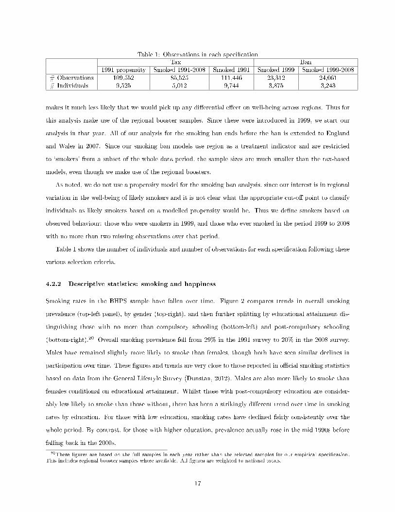
Table 1: Observations in each speci�cationTax Ban

1991 propensity Smoked 1991-2008 Smoked 1991 Smoked 1999 Smoked 1999-2008# Observations 109,552 85,525 111,446 23,312 24,061# Individuals 9,525 5,012 9,744 3,875 3,243

makes it much less likely that we would pick up any di�erential e�ect on well-being across regions. Thus for

this analysis make use of the regional booster samples. Since these were introduced in 1999, we start our

analysis in that year. All of our analysis for the smoking ban ends before the ban is extended to England

and Wales in 2007. Since our smoking ban models use region as a treatment indicator and are restricted

to `smokers' from a subset of the whole data period, the sample sizes are much smaller than the tax-based

models, even though we make use of the regional boosters.

As noted, we do not use a propensity model for the smoking ban analysis, since our interest is in regional

variation in the well-being of likely smokers and it is not clear what the appropriate cut-o� point to classify

individuals as likely smokers based on a modelled propensity would be. Thus we de�ne smokers based on

observed behaviour: those who were smokers in 1999, and those who ever smoked in the period 1999 to 2008

with no more than two missing observations over that period.

Table 1 shows the number of individuals and number of observations for each speci�cation following these

various selection criteria.

4.2.2 Descriptive statistics: smoking and happiness

Smoking rates in the BHPS sample have fallen over time. Figure 2 compares trends in overall smoking

prevalence (top-left panel), by gender (top-right), and then further splitting by educational attainment dis-

tinguishing those with no more than compulsory schooling (bottom-left) and post-compulsory schooling

(bottom-right).20 Overall smoking prevalence fell from 29% in the 1991 survey to 20% in the 2008 survey.

Males have remained slightly more likely to smoke than females, though both have seen similar declines in

participation over time. These �gures and trends are very close to those reported in o�cial smoking statistics

based on data from the General Lifestyle Survey (Dunstan, 2012). Males are also more likely to smoke than

females conditional on educational attainment. Whilst those with post-compulsory education are consider-

ably less likely to smoke than those without, there has been a strikingly di�erent trend over time in smoking

rates by education. For those with low education, smoking rates have declined fairly consistently over the

whole period. By contrast, for those with higher education, prevalence actually rose in the mid 1990s before

falling back in the 2000s.

20These �gures are based on the full samples in each year rather than the selected samples for our empirical speci�cation.This includes regional booster samples where available. All �gures are weighted to national totals.

17

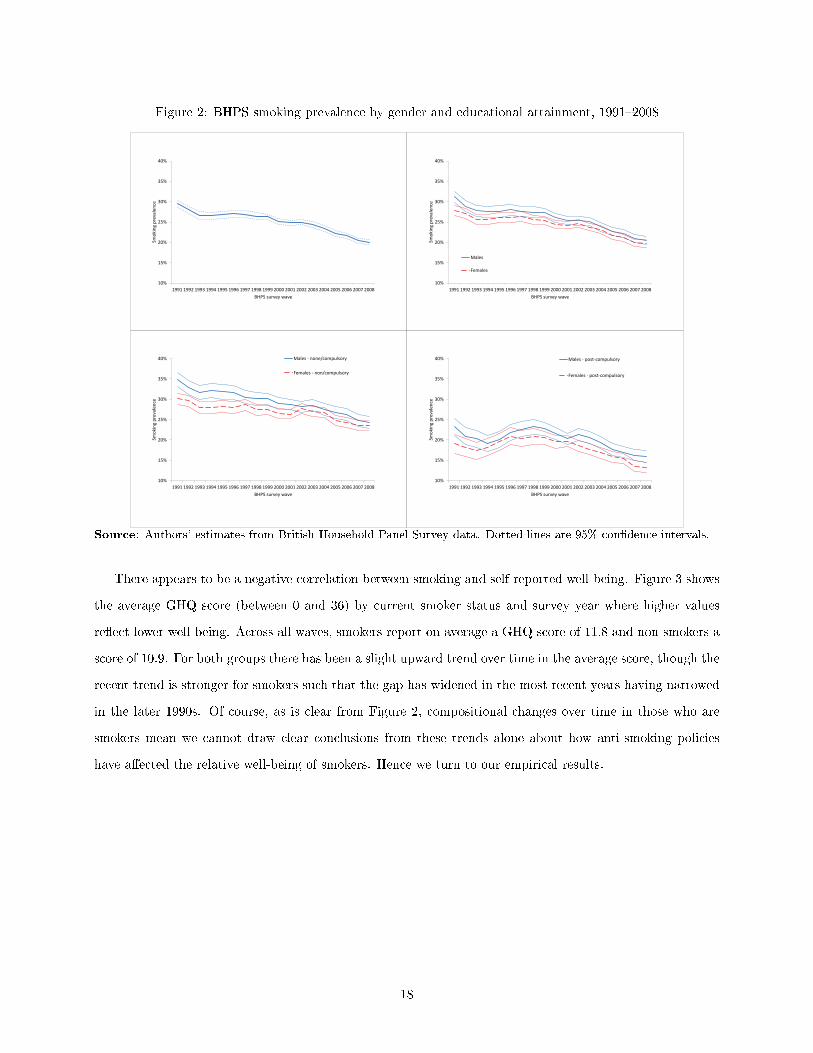
Figure 2: BHPS smoking prevalence by gender and educational attainment, 1991�2008

10%

15%

20%

25%

30%

35%

40%

1991 1992 1993 1994 1995 1996 1997 1998 1999 2000 2001 2002 2003 2004 2005 2006 2007 2008

Smok

ing

prev

alen

ce

BHPS survey wave

10%

15%

20%

25%

30%

35%

40%

1991 1992 1993 1994 1995 1996 1997 1998 1999 2000 2001 2002 2003 2004 2005 2006 2007 2008

Smok

ing

prev

alen

ce

BHPS survey wave

Males

Females

10%

15%

20%

25%

30%

35%

40%

1991 1992 1993 1994 1995 1996 1997 1998 1999 2000 2001 2002 2003 2004 2005 2006 2007 2008

Smok

ing

prev

alen

ce

BHPS survey wave

Males - none/compulsory

Females - non/compulsory

10%

15%

20%

25%

30%

35%

40%

1991 1992 1993 1994 1995 1996 1997 1998 1999 2000 2001 2002 2003 2004 2005 2006 2007 2008

Smok

ing

prev

alen

ce

BHPS survey wave

Males - post-compulsory

Females - post-compulsory

Source: Authors' estimates from British Household Panel Survey data. Dotted lines are 95% con�dence intervals.

There appears to be a negative correlation between smoking and self-reported well-being. Figure 3 shows

the average GHQ score (between 0 and 36) by current smoker status and survey year where higher values

re�ect lower well-being. Across all waves, smokers report on average a GHQ score of 11.8 and non-smokers a

score of 10.9. For both groups there has been a slight upward trend over time in the average score, though the

recent trend is stronger for smokers such that the gap has widened in the most recent years having narrowed

in the later 1990s. Of course, as is clear from Figure 2, compositional changes over time in those who are

smokers mean we cannot draw clear conclusions from these trends alone about how anti-smoking policies

have a�ected the relative well-being of smokers. Hence we turn to our empirical results.

18

Figure 3: GHQ score by current smoker status, 1991�2008

9

9.5

10

10.5

11

11.5

12

12.5

13

1991 1992 1993 1994 1995 1996 1997 1998 1999 2000 2001 2002 2003 2004 2005 2006 2007 2008

Aver

age

GHQ

scor

e (h

ighe

r = g

reat

er d

istre

ss)

BHPS survey wave

Non-smoker

Smoker

Source: Authors' estimates from British Household Panel Survey data. Dotted lines are 95% con�dence intervals.

5 Results

5.1 Cigarette excise taxes

Table 2 shows the proportion of individuals classi�ed as current smokers and as treatment and control groups

under the two speci�cations which use smoking histories to de�ne those who may bene�t from higher excise

taxes as a commitment device. It also shows the average smoking propensity score from the probit model of

smoking status using the 1991 sample for the treatment and control groups and for current smokers.

Table 2: Likely smoker variablesCurrent smoker Everyone #Observations #Individuals

Yes No No AnswerAverage pscore 0.35 0.24 0.32 0.27 113,821 9,816Ever smoked 1991-2008 100% 16% 37% 35% 86,938 5,012Smoked 1991 89% 9% 27% 29% 113,821 9,816

The table shows that the average propensity score is higher for individuals observed smoking in any given

year than those observed not smoking, though the di�erence is not huge (0.35 compared to 0.24). 35%

19

of the sample were seen smoking at one point in our sample and are included in our ever smoked group.

Interestingly, only 16% of those observed not smoking in any given year are seen smoking on some other

occasion, suggesting that most non-smokers are essentially never smokers. 29% of the sample were seen

smoking in the �rst year of data in 1991.

All of the well-being equations include year dummies,21 the smoker status variable (the treatment/control

indicator or the propensity score) and its interaction with the real excise tax rate (measured in pounds per

pack of 20 cigarettes), and the same set of covariates as the smoking propensity model. As discussed earlier,

these covariates serve merely as controls in the model. For reasons of space we do not therefore present the

full model results, and instead present the key results of interest. Full results are available on request.

Table 3 shows results from an OLS speci�cation where the overall GHQ score (on the 0-36 scale) is the

dependent variable. Recall that higher GHQ scores re�ect lower well-being; as a result, if higher excise

taxes were associated with an increase in the relative well-being of the smoker groups we would expect a

negative coe�cient on the interaction term. Each column shows a di�erent speci�cation of the de�nition of

the `smoker' variable as outlined above. Column (1) shows a naive speci�cation using current smoker status,

likely to be endogenous to the current tax rate. Column (2) replaces current status with the propensity score

based on the 1991 smoker probit. Column (3) replaces current smoker status with a treatment indicator set

to 1 for those who were smokers at any time between 1991 and 2008. Column (4) sets the treatment indicator

to 1 for those who smoked in 1991.

Table 3: Cigarette taxes and smoker well-being: overall GHQ score(1) (2) (3) (4)

Current smoker 1991 propensity Smoked 1991-2008 Smoked 1991`Smoker' e�ect 0.657*** 4.376*** 0.796*** 0.880***

(0.229) (1.168) (0.235) (0.212)Cigarette tax 1.224** 1.273** 0.905 1.264**

(0.613) (0.620) (0.751) (0.613)Interaction -0.126* -0.243 -0.199*** -0.230***

(0.075) (0.246) (0.070) (0.068)Observations 111,399 109,552 85,525 111,446Individuals 9,744 9,525 5,012 9,744R2 0.176 0.173 0.176

Clustered (on the individual) standard errors in parentheses. Standard errors in Column (2) are based on 1,000 bootstrap replications.

* p < 0.10 , ** p < 0.05 , *** p < 0.01

Being a smoker, or a likely smoker based on individual characteristics or observed behaviour, is consistently

related to lower overall well-being. Smokers in the two treatment/control speci�cations (columns 3 and 4)

have average GHQ scores around 0.8 to 0.9 points higher than non-smokers. It is hard to compare that to the

21We do not control speci�cally for month - whilst we may expect seasonal variation in reported well-being, recall that almostall the interviews in the BHPS take place between September and November in a given year.

20

propensity score speci�cation (column 2) since here the `smoker' variable is just the propensity score in the

range 0 to 1. Taking the average observed propensity score for current smokers in the sample (0.36) compared

to the average propensity score for non-smokers (0.25) and multiplying the di�erence by the coe�cient gives

that an average smoker in this speci�cation has a GHQ score around 0.5 points higher than an average

non-smoker.

Increases in real cigarette taxes also tend to raise GHQ scores (reduce well-being): a ¿1 tax rise is

assocated with an average increase of around 1 to 1.2 points in the GHQ score, though this is not statistically

signi�cant in all speci�cations.

The interaction terms are consistently negative, though the statistical signi�cance varies across speci�ca-

tions, being strongly signi�cant for the treatment/control models but not signi�cant in the propensity score

model. These results lend some support to the view that a treatment group of smokers sees their well-being

rise relative to a control group of non-smokers as taxes increase (though note that the overall e�ect of higher

taxes on `smoker' well-being given by the sum of the tax and interaction terms is still negative). Taking the

treatment/control speci�cations, for example, a ¿1 rise in taxes would be associated with a relative fall in

the GHQ score of smokers of around 0.2 points. This compares to an average GHQ score for the sample of

11.1 and a standard deviation of 5.3.

As discussed in Section 4.1, an open empirical question is whether poorer consumers exhibit a greater

degree of time inconsistency. If so, one implication is that low education smokers (where low education is a

proxy for low lifetime income) would see the largest bene�ts from the commitment value of higher taxation.

Table 4 repeats the analysis, further interacting the smoker status and tax interaction with three educational

attainment groups (post-compulsory, compulsory only and no formal quali�cations). The interaction terms

are all negative, though vary across speci�cations in terms of stastistical signi�cance. The results point in

the direction that those with compulsory education see larger bene�ts from higher taxes than those with

post-compulsory education, but also larger bene�ts than those with no formal quali�cations. However it is

possible that the `no quali�cation' group also tend to be older, possibly con�ating age and education e�ects.

Further, the degree of statistical signi�cance of the di�erences across education groups is limited: F-tests

fail to reject the null hypothesis that all the interaction coe�cients are the same except in the speci�cation

de�ning treatment status based on observed smoking behaviour between 1991 and 2008 (column 3). Thus

there is relatively little compelling evidence for greater time inconsistency among the lifetime poor from these

results.

21

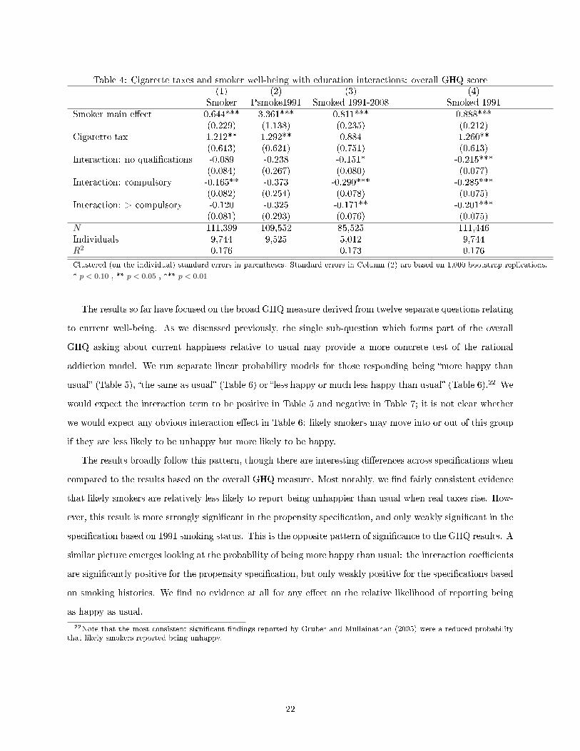
Table 4: Cigarette taxes and smoker well-being with education interactions: overall GHQ score(1) (2) (3) (4)

Smoker Psmoke1991 Smoked 1991-2008 Smoked 1991Smoker main e�ect 0.644*** 3.361*** 0.811*** 0.888***

(0.229) (1.138) (0.235) (0.212)Cigarette tax 1.212** 1.292** 0.884 1.260**

(0.613) (0.621) (0.751) (0.613)Interaction: no quali�cations -0.089 -0.238 -0.151* -0.215***

(0.084) (0.267) (0.080) (0.077)Interaction: compulsory -0.165** -0.373 -0.290*** -0.285***

(0.082) (0.254) (0.078) (0.075)Interaction: > compulsory -0.120 -0.325 -0.171** -0.201***

(0.081) (0.293) (0.076) (0.075)N 111,399 109,552 85,525 111,446Individuals 9,744 9,525 5,012 9,744R2 0.176 0.173 0.176

Clustered (on the individual) standard errors in parentheses. Standard errors in Column (2) are based on 1,000 bootstrap replications.

* p < 0.10 , ** p < 0.05 , *** p < 0.01

The results so far have focused on the broad GHQ measure derived from twelve separate questions relating

to current well-being. As we discussed previously, the single sub-question which forms part of the overall

GHQ asking about current happiness relative to usual may provide a more concrete test of the rational

addiction model. We run separate linear probability models for those responding being �more happy than

usual� (Table 5), �the same as usual� (Table 6) or �less happy or much less happy than usual� (Table 6).22 We

would expect the interaction term to be positive in Table 5 and negative in Table 7; it is not clear whether

we would expect any obvious interaction e�ect in Table 6: likely smokers may move into or out of this group

if they are less likely to be unhappy but more likely to be happy.

The results broadly follow this pattern, though there are interesting di�erences across speci�cations when

compared to the results based on the overall GHQ measure. Most notably, we �nd fairly consistent evidence

that likely smokers are relatively less likely to report being unhappier than usual when real taxes rise. How-

ever, this result is more strongly signi�cant in the propensity speci�cation, and only weakly signi�cant in the

speci�cation based on 1991 smoking status. This is the opposite pattern of signi�cance to the GHQ results. A

similar picture emerges looking at the probability of being more happy than usual: the interaction coe�cients

are signi�cantly positive for the propensity speci�cation, but only weakly positive for the speci�cations based

on smoking histories. We �nd no evidence at all for any e�ect on the relative likelihood of reporting being

as happy as usual.

22Note that the most consistent signi�cant �ndings reported by Gruber and Mullainathan (2005) were a reduced probabilitythat likely smokers reported being unhappy.

22

Table 5: Relationship between cigarette taxes and being more happy than usual(1) (2) (3) (4)

Current smoker 1991 propensity Smoked 1991-2008 Smoked 1991`Smoker' e�ect -0.012 -0.163*** -0.030** -0.026**

(0.012) (0.053) (0.014) (0.012)Cigarette tax 0.023 0.015 0.022 0.020

(0.041) (0.041) (0.051) (0.041)Interaction 0.000 0.031** 0.008* 0.006*

(0.004) (0.013) (0.004) (0.004)Observations 113,770 113,821 86,938 113,821Individuals 9,816 9,816 5,012 9,816R2 0.025 0.025 0.025

Clustered (on the individual) standard errors in parentheses. Standard errors in Column (2) are based on 1,000 bootstrap replications.

* p < 0.10 , ** p < 0.05 , *** p < 0.01

Table 6: Relationship between cigarette taxes and being the same happiness as usual(1) (2) (3) (4)

Current smoker 1991 propensity Smoked 1991-2008 Smoked 1991`Smoker' e�ect -0.005 -0.046 -0.002 0.002

(0.017) (0.078) (0.019) (0.016)Cigarette tax -0.106* -0.105* -0.077 -0.106*

(0.055) (0.054) (0.066) (0.054)Interaction 0.002 -0.002 -0.000 -0.001

(0.005) (0.017) (0.006) (0.005)Observations 113,770 113,821 86,938 113,821Individuals 9,816 9,816 5,012 9,816R2 0.060 0.062 0.060

Clustered (on the individual) standard errors in parentheses. Standard errors in Column (2) are based on 1,000 bootstrap replications.

* p < 0.10 , ** p < 0.05 , *** p < 0.01

Table 7: Relationship between cigarette taxes and being less happy than usual(1) (2) (3) (4)

Current smoker 1991 propensity Smoked 1991-2008 Smoked 1991`Smoker' e�ect 0.023* 0.217*** 0.039*** 0.029**

(0.013) (0.059) (0.015) (0.013)Cigarette tax 0.063 0.068 0.063 0.064

(0.041) (0.042) (0.050) (0.041)Interaction -0.004 -0.027** -0.010** -0.007*

(0.004) (0.014) (0.004) (0.004)Observations 113,770 113,821 86,938 113,821Individuals 9,816 9,816 5,012 9,816R2 0.083 0.085 0.083

Clustered (on the individual) standard errors in parentheses. Standard errors in Column (2) are based on 1,000 bootstrap replications.

* p < 0.10 , ** p < 0.05 , *** p < 0.01

In summary, the results based on the single happiness question point in the same direction as the results

based on the overall GHQ measure: likely smokers appear to be made relatively better o� from higher

real excise taxes. Taxes had a negative and signi�cant e�ect on the relative distress of likely smokers for

23

two out of three of the treatment groups at the 5% level; in the third case the sign of the e�ect was also

negative. For all speci�cations, treatment groups were more likely to report being happier than usual and less

likely to report being unhappier than usual with at least 10% signi�cance. Although the magnitude of the

interaction term is quite low relative to the mean or standard deviation of happiness measures, the fact that

they all point consistently in the same direction is noteworthy, and goes against the prediction of the rational

addiction model. We �nd only very weak evidence that the e�ect is greater for low education individuals in

the treatment group.

5.2 Ban on smoking in public places

For the analysis of regional variation in the timing of the smoking ban, the sample is restricted to those

classi�ed as likely smokers, comparing the well-being of smokers in Scotland to England and Wales in the

period following the ban being implemented north of the border. We restrict our sample to stop in March 2007,

before the ban is extended to other regions. We show results for the speci�cation classifying likely smokers

based on their 1999 smoking behaviour. Results from the alternative strategy outlined above drawing on

observed smoking status over the whole period 1999 to 2008 are quantitatively very similar and are available

on request.

As always with di�erence-in-di�erence studies, we make the common trend assumption. This means that

changes in likely smoker well-being in England and Wales would be a good predictor of changes in Scotland

absent the smoking ban having been implemented there. Figure 4 shows trends in the average GHQ score

by region (Scotland versus England and Wales) and year among those who smoked in 1999. The trends

are broadly similar: �at or declining GHQ scores in both regions up to around 2003 with some evidence of

increasing scores (reduced well-being) since then. The striking di�erence is 1999 to 2000 when there was a

large increase in the GHQ score in England and Wales not seen in Scotland.

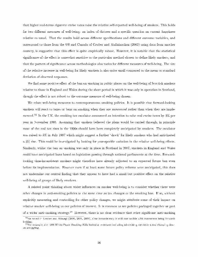
Table 8 shows the main results, again focused on the coe�cients of key interest: the coe�cient on the

Scotland dummy, a dummy for the period between March 2006 and March 2007 (when the ban is in place

in Scotland but not elsewhere) and the interaction term between the two which is the di�erence-in-di�erence

estimate. Columns here represent di�erent dependent variables: linear probability models for the three

categorical responses to the single happiness equation and an OLS model for the overall GHQ index.

While we �nd no sign�cant e�ects of the ban on the relative probability of a smoker being more, less,

or no more happy than usual, we do �nd signi�cant e�ects of the ban on the overall GHQ score of those

who were seen smoking in 1999. According to the results in column 4, the smoking ban appears to have

improved well-being for likely smokers in Scotland by around 0.5 points relative to likely smokers in England

24

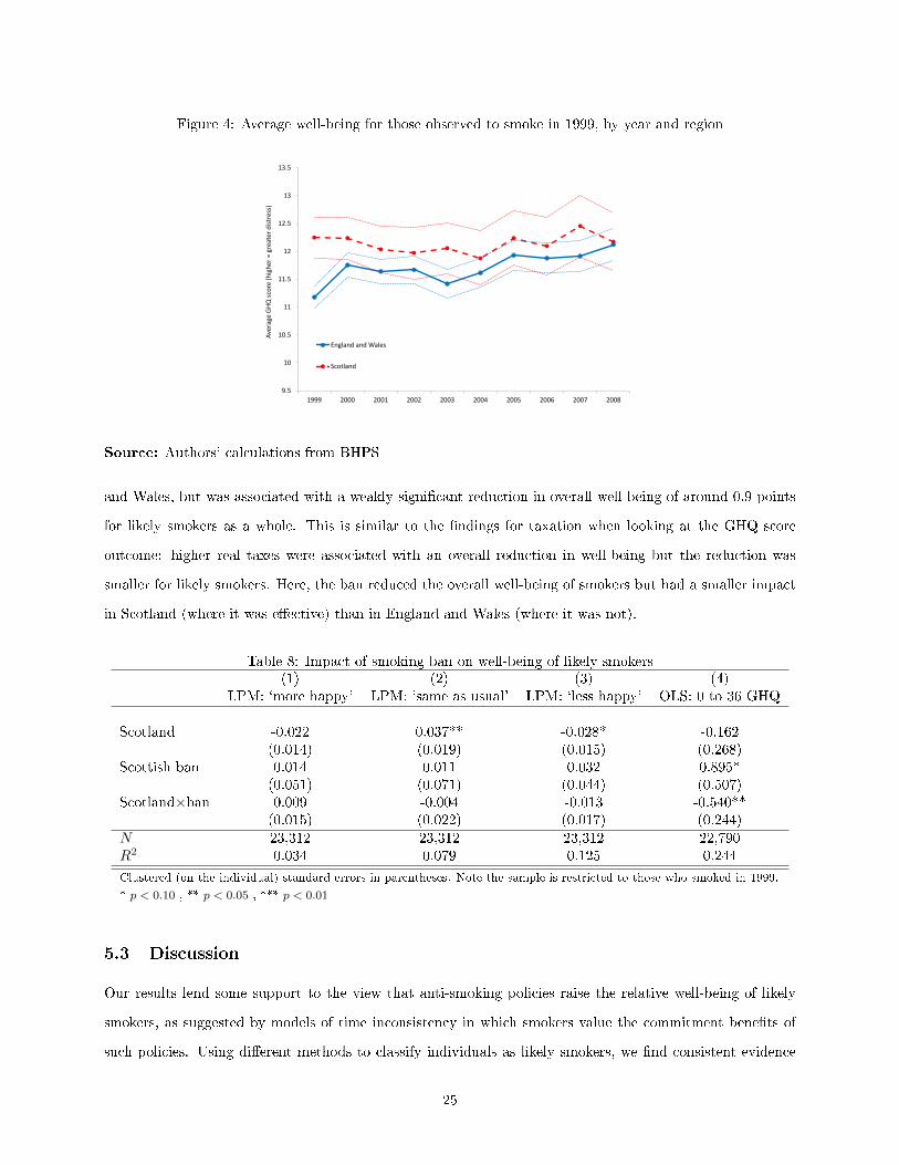
Figure 4: Average well-being for those observed to smoke in 1999, by year and region

9.5

10

10.5

11

11.5

12

12.5

13

13.5

1999 2000 2001 2002 2003 2004 2005 2006 2007 2008

Aver

age

GHQ

scor

e (h

ighe

r = g

reat

er d

istre

ss)

England and Wales

Scotland

Source: Authors' calculations from BHPS

and Wales, but was associated with a weakly signi�cant reduction in overall well-being of around 0.9 points

for likely smokers as a whole. This is similar to the �ndings for taxation when looking at the GHQ score

outcome: higher real taxes were associated with an overall reduction in well-being but the reduction was

smaller for likely smokers. Here, the ban reduced the overall well-being of smokers but had a smaller impact

in Scotland (where it was e�ective) than in England and Wales (where it was not).

Table 8: Impact of smoking ban on well-being of likely smokers(1) (2) (3) (4)

LPM: `more happy' LPM: `same as usual' LPM: `less happy' OLS: 0 to 36 GHQ

Scotland -0.022 0.037** -0.028* -0.162(0.014) (0.019) (0.015) (0.268)

Scottish ban 0.014 0.011 0.032 0.895*(0.051) (0.071) (0.044) (0.507)

Scotland×ban 0.009 -0.004 -0.013 -0.540**(0.015) (0.022) (0.017) (0.244)

N 23,312 23,312 23,312 22,790R2 0.034 0.079 0.125 0.244

Clustered (on the individual) standard errors in parentheses. Note the sample is restricted to those who smoked in 1999.

* p < 0.10 , ** p < 0.05 , *** p < 0.01

5.3 Discussion

Our results lend some support to the view that anti-smoking policies raise the relative well-being of likely

smokers, as suggested by models of time inconsistency in which smokers value the commitment bene�ts of

such policies. Using di�erent methods to classify individuals as likely smokers, we �nd consistent evidence

25

that higher real-terms cigarette excise taxes raise the relative self-reported well-being of smokers. This holds

for two di�erent measures of well-being: an index of distress and a speci�c question on current happiness

relative to usual. That the results hold across di�erent speci�cations and di�erent outcome variables, and

correspond to those from the US and Canada of Gruber and Mullainathan (2005) using data from another

country, is suggestive that this e�ect is quite empirically robust. However, it is notable that the statistical

signi�cance of the e�ect is somewhat sensitive to the particular method chosen to de�ne likely smokers, and

that the pattern of signi�cance across methodologies also varies for di�erent measures of well-being. The size

of the relative increase in well-being for likely smokers is also quite small compared to the mean or standard

deviation of observed responses.

We �nd some positive e�ect of the ban on smoking in public places on the well-being of Scottish smokers

relative to those in England and Wales during the short period in which it was only in operation in Scotland,

though the e�ect is not robust to the outcome measure of well-being chosen.

We relate well-being measures to contemporaneous smoking policies. It is possible that forward-looking

smokers will react to taxes or bans on smoking when they are announced rather than when they are imple-

mented.23 In the UK, the smoking tax escalator announced an intention to raise real excise taxes by 3% per

year in November 1993. Assuming that smokers believed the plans would be carried through, in principle

most of the real tax rises in the 1990s should have been completely anticipated by smokers. The escalator

was raised to 5% in July 1997 which might suggest a further `shock' for likely smokers who had anticipated

a 3% rise. This could be investigated by looking for year-speci�c variation in the relative well-being e�ects.

Similarly, whilst the ban on smoking was only in place in Scotland in 2007, smokers in England and Wales

could have anticipated bans based on legislation passing through national parliaments at the time. Forward-

looking time-inconsistent smokers might therefore have already adjusted to an expected future ban even

before its implementation. However even if at least some future policy reforms were anticipated, this does

not undermine our central �nding that they appear to have had a small but positive e�ect on the relative

well-being of groups of likely smokers.

A related point thinking about wider in�uences on smoker well-being is to consider whether there were

other changes in anti-smoking policies at the same time as tax changes or the smoking ban. If so, without

explicitly measuring and controlling for other policy changes, we might attribute some of their impact on

relative smoker well-being to our policies of interest. It is common to see policies packaged together as part

of a wider anti-smoking strategy.24 However, there is no clear evidence that other signi�cant anti-smoking

23As noted in Gruber and K®szegi (2000, 2001, 2004), time inconsistency is still compatible with consumers being forward-looking.

24For example, the 1998 White Paper Smoking Kills looked at measures including advertising restrictions and clamping downon smuggling.

26

reforms were introduced at the same time as the main increase in real excise taxes in the 1990s under the

duty escalator. Cigarette advertising had been banned on UK television since 1965, and advertising in other

media was progressively banned between 2003 and 2005 as part of the Tobacco Advertising and Promotions

Act 2002, following the end of the escalator period. Health warnings on cigarette packets were introduced

compulsorily in July 1991, before the excise escalator, and increased in prominence and visibility from 2002,

after the escalator had ended. The legal purchase age for cigarettes was also raised after the escalator period,

in October 2007.

An alternative explanation for our results is that taxes a�ect the well-being of smokers through their

e�ects on the illicit (untaxed) market for tobacco. As noted above, illicit tobacco appeared to command

a relatively high share of the market in the 1990s when tax rates were increasing rapidly. If tax increases

lead to a rise in the availability of illicit tobacco, this could actually reduce the cost of smoking and make

smokers better o� even under a time consistent framework. This would undermine the power of our test to

discriminate between time inconsistentcy and rational addiction. Note, though, that for this to hold would

require the cost of obtaining tobacco to fall when the tax rate went up, where the cost of illicit tobacco

includes not only the purchase price but also the costs of obtaining it (which may include the hassle of

dealing with illicit sellers and any moral costs). In general, we might expect that people turning to illicit

tobacco might be paying more than they had paid for tobacco before the tax increase, just less than the cost

of obtaining licit (duty-paid) tobacco following the tax rise. However, it is possible that the cost of smoking

fell as a result of tax increases if, for instance, the growth in the size of the illicit market allowed tobacco

smugglers to bene�t from economies of scale, or if more widespread use of illict tobacco reduced any social

stigma or moral costs from consuming it. It is of course hard to determine whether these sorts of e�ects exist

or how important they are without data on who smokes illicit tobacco and how the price of licit and illicit

products changed over this period.

A �nal potential concern is attrition from our panel. Attrition may be in�uenced by both happiness and

smoking behaviour, and if there is any interaction between these e�ects it could bias our results (for example,

if relatively unhappy smokers are more likely to die or attrit from the sample for other reasons, then we

may see an upward trend in the relative happiness of smokers which correlates with the trend in real excise

taxes). To check the robustness of our results to problems of attrition, we repeat our analysis from Table 3 for

our �Smoked 1991-2008� and �Smoked 1991� measures on a sample which conditions on individuals who are

observed in all years of data. This reduces our sample sizes substantially: for example, using 1991 smoking

status to classify treated individuals, the number of observations falls by around 45% and the number of

individuals by around 64%. Using the GHQ index measure of well-being, we still �nd negative interaction

e�ects between smoker status and the real excise tax for both speci�cations (-0.17 and -0.09 respectively),

27

with the former signi�cant at the 5% level but the latter no longer statistically signi�cant. Thus we continue

to �nd the negative interaction term, but we have much less precise estimates. It is possible that an attrition

bias explains some part of our �nding, but at least for some speci�cations the result appears robust to a

sample where attrition is ruled out - even when that also entails a substantial reduction in sample size.

6 Conclusions

When people su�er from time inconsistency problems that lead them to over-consume harmful products,

policies that restrict their behaviour can in principle make them individually better o�. We �nd quite

strong evidence of such an e�ect of tobacco taxes using British panel data recording smoking status and

self-reported measures of well-being over a long period. There is also weaker evidence of a similar e�ect for a

ban on smoking in public places introduced in Scotland. We �nd little compelling evidence that the relative

e�ect is larger for poorer households as measured by educational attainment. The size of the e�ect appears

to be fairly modest, but is robust to di�erent treatment indicators and measures of well-being, and points in

the opposite direction to the predictions of standard theory.

From a policy perspective, our �ndings suggest a possible `internality' rationale for tobacco taxation as

well as the more usual externality rationale. This could suggest that optimal tobacco excise taxes exceed

those which would be justi�ed by estimates of the marginal external cost imposed on others, though we are

unable to quantify the size of the internality on the basis of our results. Drawing on a theoretical framework,

Gruber and K®szegi (2001) estimated the internality-correcting tax could be around $1 per pack of cigarettes

compared to an excise tax at the time of around 65 cents. They also argued that if poorer individuals were

more likely to su�er from time inconsistency, increases in taxes could be progressive in terms of the welfare

impact. However we �nd no signi�cant evidence that this is the case: tax do not appear to have a larger

relative e�ect on the well-being of poorer (low education) smokers than richer (high education) smokers.

References

[1] Adda, J. and F. Cornaglia (2006), �Taxes, cigarette consumption and smoking intensity�, American

Economic Review, 96 (4), 1013�28

[2] Adda, J. and F. Cornaglia (2010), �The e�ect of bans and taxes on passive smoking�, American Economic

Journal: Applied Economics, 2 (1), 1�32

[3] Ai, C. and E. Norton (2003), �Interaction terms in logit and probit models�, Economics Letters, 80 (1),

123�9

28

[4] Anger, S., M. Kvasnicka and T. Siedler (2011), �One last pu�? Public smoking bans and smoking

behaviour�, Journal of Health Economics, 30, 591�601

[5] Badillo Amador, L. and López Nicolás, Á (2011), �Self-control and support for anti-smoking policies

among smokers, ex smokers and never smokers�, European Journal of Health Economics, October

[6] Bardasi, E., S. Jenkins, H. Sutherland, H. Levy and F. Zantomio (2012), British Household Panel Survey

Derived Current and Annual Net Household Income Variables, Waves 1-18, 1991-2009 (9th Edition),

University of Essex Institute for Social and Economic Research (original data producers), Colchester,

Essex; UK Data Archive (distributor), SN 3909 (http://dx.doi.org/10.5255/UKDA-SN-3909-2)

[7] de Bartolome, C. and I. Irvine (2010), The Economics of Smok-

ing Bans, University College Dublin Geary Institute Discussion Paper

(http://www.ucd.ie/geary/static/publications/workingpapers/gearywp201027.pdf)

[8] Becker, G. and K. Murphy (1988), �A theory of rational addiction�, Journal of Political Economy, 96

(4), 675�700

[9] Bernheim, B. and A. Rangel (2004), �Addiction and cue-triggered decision processes�, American Eco-

nomic Review, 94 (5), 1558�90

[10] Bernheim, B. and A. Rangel (2005), Behavioral Public Economics: Welfare and Policy Analysis with

Non-Standard Decision-Makers, NBER Working Paper 11518 (http://www.nber.org/papers/w11518)

[11] Brodeur, A. (2013), Smoking, Income and Subjective Well-Being: Evidence from Smoking Bans, mimeo,

Paris School of Economics (http://cep.lse.ac.uk/pubs/download/dp1202.pdf)

[12] Bryan, G., D. Karlan and S. Nelson (2010), �Commitment devices�, Annual Review of Economics, 2,

671�98

[13] Carpenter, C., S. Postolek and C. Warman (2011), �Public-place smoking laws and exposure to environ-

mental tobacco smoke (ETS)�, American Economic Journal: Economic Policy, 3, 35�61

[14] Chaloupka, F. and K. Warner (2000), �The economics of smoking�, in Culyer, A. and J. Newhouse (eds.),

Handbook of Health Economics, Volume 1

[15] Choi, S., S. Kariv, W. Müller and D. Silverman (2011), Who is (More) Rational?, Working Paper

(http://www.homepages.ucl.ac.uk/∼uctpsc0/Research/CKMS_I.pdf)

[16] Clark, A. and F. Etilé (2002), �Do health changes a�ect smoking? Evidence from British panel data�,

Journal of Health Economics, 21 (4), 533�62

29

[17] Clark, E. and A. Oswald (2002), �A simple statistical method for measuring how life events a�ect

happiness�, International Journal of Epidemiology, 31 (6), 1139�44

[18] Crawford, I., M. Keen and S. Smith (2010), �Value Added Tax and excises�, in Mirrlees, J., S.

Adam, T. Besley, R. Blundell, S. Bond, R. Chote, M. Gammie, P. Johnson, G. Myles and J.

Poterba (eds.), Dimensions of Tax Design: the Mirrlees Review, Oxford: Oxford University Press

(http://www.ifs.org.uk/mirrleesreview/dimensions/ch4.pdf)

[19] DellaVigna, S. (2009), �Psychology and economics: evidence from the �eld�, Journal of Economic Lit-

erature, 47 (2), 315�72

[20] Dunstan, S. (ed.) (2012), General Lifestyle Survey Overview: a Report on the 2010 General Lifestyle

Survey, London: O�ce for National Statistics (http://www.ons.gov.uk/ons/rel/ghs/general-lifestyle-

survey/2010/index.html)

[21] Evans, W. and M. Farrelly (1998), �The compensating behavior of smokers: taxes, tar and nicotine�,

RAND Journal of Economics, 29 (3), 578�95

[22] Farrelly, M., C. Nimsch, A. Hyland and M. Cummings (2004), �The e�ects of higher cigarette prices on

tar and nicotine consumption in a cohort of adult smokers�, Health Economics, 13, 49�58

[23] Frederick, S., G. Loewenstein and T. O'Donoghue (2002), �Time discounting and time preference: a

critical review�, Journal of Economic Literature, 40 (2), 351�401

[24] Gallet, C. and J. List (2003), �Cigarette demand: a meta-analysis of elasticities�, Health Economics, 12,

821�35

[25] Goldberg, D. (1972), The Detection of Psychiatric Illness by Questionnaire, London: Oxford University

Press

[26] Gruber, J. and B. K®szegi (2000), Is addiction `rational'? Theory and evidence, NBER Working Paper

7507 (http://www.nber.org/papers/w7507.pdf)

[27] Gruber, J. and B. K®szegi (2001), �Is addiction `rational'? Theory and evidence�, Quarterly Journal of

Economics, 116 (4), 1261�1303

[28] Gruber, J. and B. K®szegi (2004), �Tax incidence when individuals are time-inconsistent: the case of

cigarette excise taxes�, Journal of Public Economics, 88 (9�10), 1959�87

[29] Gruber, J. and S. Mullainathan (2005), �Do cigarette taxes make smokers happier�, Advances in Eco-

nomic Analysis & Policy, 5 (1), Article 4

30

[30] Gruber, J. and J. Zinman (2001), �Youth smoking in the United States: evidence and implications�, in

J. Gruber (ed.), Risky Behavior among Youths: An Economic Analysis, Chicago: University of Chicago

Press (http://www.nber.org/chapters/c10687.pdf)

[31] Gul, F. and W. Pesendorfer (2001), �Temptation and self-control�, Econometrica, 69 (6), 1403�36

[32] Gul, F. and W. Pesendorfer (2007), �Harmful addiction�, Review of Economic Studies, 74 (1), 147�72

[33] Hersch, J. (2005), �Smoking restrictions as a self-control mechanism�, Journal of Risk and Uncertainty,

31 (1), 5�21

[34] HMCE and HMT (2000), Tackling Tobacco Smuggling, London: The Stationery O�ce Limited

(http://www.hm-treasury.gov.uk/d/433.pdf)

[35] HMRC (2011a), Tobacco Duties Factsheet November 2011, London: HMRC

(https://www.uktradeinfo.com/Statistics/Statistical%20Factsheets/TobaccoFactsheet2011.xls)

[36] HMRC (2011b), Measuring Tax Gaps 2011, London: HMRC (http://www.hmrc.gov.uk/stats/mtg-

2011.pdf)

[37] HMRC (2012), Tobacco duty bulletin July 2012, London: HMRC

(https://www.uktradeinfo.com/Statistics/Tax%20and%20Duty%20Bulletins/Tob0712.xls)

[38] Hopkins, D., S. Razi, K. Leeks, G. Kalra, S. Chattopadhyay and R. Soler (2010), �Smokefree policies to

reduce tobacco use�, American Journal of Preventive Medicine, 38 (2S), S275�89

[39] Jehiel, P. and A. Lilico (2010), �Smoking today and stopping tomorrow: a limited foresight perspective�,

CESifo Economic Studies, 56 (2), 141�64

[40] Jones, A., A. Laporte, N. Rice and E. Zucchelli (2011), A Model of the Impact of Smoking Bans on

Smoking With Evidence from Bans in England and Scotland, University of York Health, Econometrics

and Data Group Working Paper W05/11 (http://www.york.ac.uk/res/herc/documents/wp/11_05.pdf)

[41] Kan, K. (2007), �Cigarette smoking and self-control�, Journal of Health Economics, 26 (1), 61�81

[42] Laibson, D. (1997), �Golden eggs and hyperbolic discounting�, Quarterly Journal of Economics, 112 (2),

443�77

[43] Larsen, R. and B. Fredrickson (1999), �Measurement issues in emotion research�, in Kahneman, D., E.

Diener and N. Schwarz (eds.), Well-Being: Foundations of Hedonic Psychology, New York: Russell Sage

(http://www.unc.edu/peplab/publications/Larsen%20&%20Fredrickson_1999.pdf)

31

[44] Loewenstein, G., T. O'Donoghue and M. Rabin (2003), �Projection bias in predicting future utility�,

Quarterly Journal of Economics, 118 (4), 1209�48

[45] Moore, S. (2009), �The nonpecuniary e�ects of smoking cessation: happier smokers smoke less�, Applied

Economics Letters, 16 (4), 395�8

[46] NHS Information Centre (2012), Statistics on Smoking - England, 2012, Data Tables (avail-

able from http://www.ic.nhs.uk/statistics-and-data-collections/health-and-lifestyles/smoking/statistics-

on-smoking�england-2012)

[47] O'Donoghue, T. and M. Rabin (1999), �Doing it now or later�, American Economic Review, 89 (1),

103�24

[48] Odermatt, R. and Stutzer, A. (2012), Smoking Bans and Life Satisfaction in Europe, mimeo

(http://www.iza.org/conference_�les/ReDisWeBe2010/odermatt_r6632.pdf)

[49] Orphanides, A. and D. Zervos (1995), �Rational addiction with learning and regret�, Journal of Political

Economy, 103 (4), 739�58

[50] Oswald, A. (1997), �Happiness and economic performance�, Economic Journal, 107 (445), 1815�31

[51] Paserman, M. (2008), �Job search and hyperbolic discounting: structural estimation and policy evalua-

tion�, Economic Journal, 118 (531), 1418�52

[52] Schoenbaum, M. (2005), �The accuracy of teens' expectations of future smoking�, American Journal of

Preventive Medicine, 28 (3), 274�80

[53] Shetty, K., T. DeLeire, C. White and J. Bhattacharya (2009), Changes in U.S. Hospitalization and

Mortality Rates Following Smoking Bans, NBER Working Paper 14790

[54] Sloan, F. and A. Platt (2011), �Information, risk perceptions, and smoking choices of youth�, Journal of

Risk and Uncertainty, 42, 161�93

[55] Stehr, M. (2005), �Cigarette tax avoidance and evasion�, Journal of Health Economics, 24, 277�97

[56] Stutzer, A. and B. Frey (2010), Recent Advances in the Economics of Individual Subjective Well-Being,

IZA Discussion Paper 4850 (http://ftp.iza.org/dp4850.pdf)

[57] Suranovic, S., R. Goldfarb and T. Leonard (1999), �An economic theory of cigarette addiction�, Journal

of Health Economics, 18 (1), 1�29

32

Appendix: Propensity to smoke results

Table 9: Smoker Probit, 1991

(1)

Dep var: Smoker

Age 0.0461∗∗∗

(7.96)

Age2 -0.000638∗∗∗

(-10.14)

Female -0.128∗∗∗

(-4.16)

Child 0-4 0.0469

(0.90)

More than one child 0-4 0.0279

(0.33)

Child 5-11 0.114∗

(2.39)

More than one child 5-11 -0.0714

(-1.19)

Child 12-18 -0.0878

(-1.89)

More than one child 12-18 -0.351∗∗∗

(-5.11)

2nd income decile -0.0631

(-0.86)

3rd income decile -0.175∗

(-2.38)

4th income decile -0.150∗

(-2.09)

5th income decile -0.254∗∗∗

(-3.57)

33

6th income decile -0.192∗∗

(-2.70)

7th income decile -0.329∗∗∗

(-4.54)

8th income decile -0.221∗∗

(-3.02)

9th income decile -0.170∗

(-2.27)

10th income decile -0.389∗∗∗

(-4.94)

Income decile -0.126

(-1.77)

No formal quali�cation 0.731∗∗∗

(4.84)

O-level/CSE 0.553∗∗∗

(3.66)

A-level 0.332∗

(2.17)

Undergraduate 0.146

(0.94)

Self-employed 0.0301

(0.55)

Retired 0.109

(1.68)

Unemployed 0.250∗∗∗

(3.98)

Other employment -0.116∗∗

(-2.58)

Student 0.170

(1.90)

Co-habiting 0.298∗∗∗

(5.01)

34

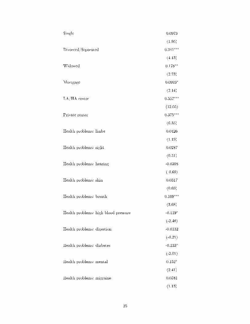
Single 0.0973

(1.95)

Divorced/Separated 0.241∗∗∗

(4.13)

Widowed 0.178∗∗

(2.73)

Mortgage 0.0923∗

(2.14)

LA/HA renter 0.557∗∗∗

(12.05)

Private renter 0.375∗∗∗

(6.35)

Health problems: limbs 0.0426

(1.19)

Health problems: sight 0.0287

(0.51)

Health problems: hearing -0.0398

(-0.69)

Health problems: skin 0.0317

(0.69)

Health problems: breath 0.169∗∗∗

(3.68)

Health problems: high blood pressure -0.119∗

(-2.48)

Health problems: digestion -0.0132

(-0.21)

Health problems: diabetes -0.233∗

(-2.01)

Health problems: mental 0.152∗

(2.41)

Health problems: migraine 0.0581

(1.13)

35

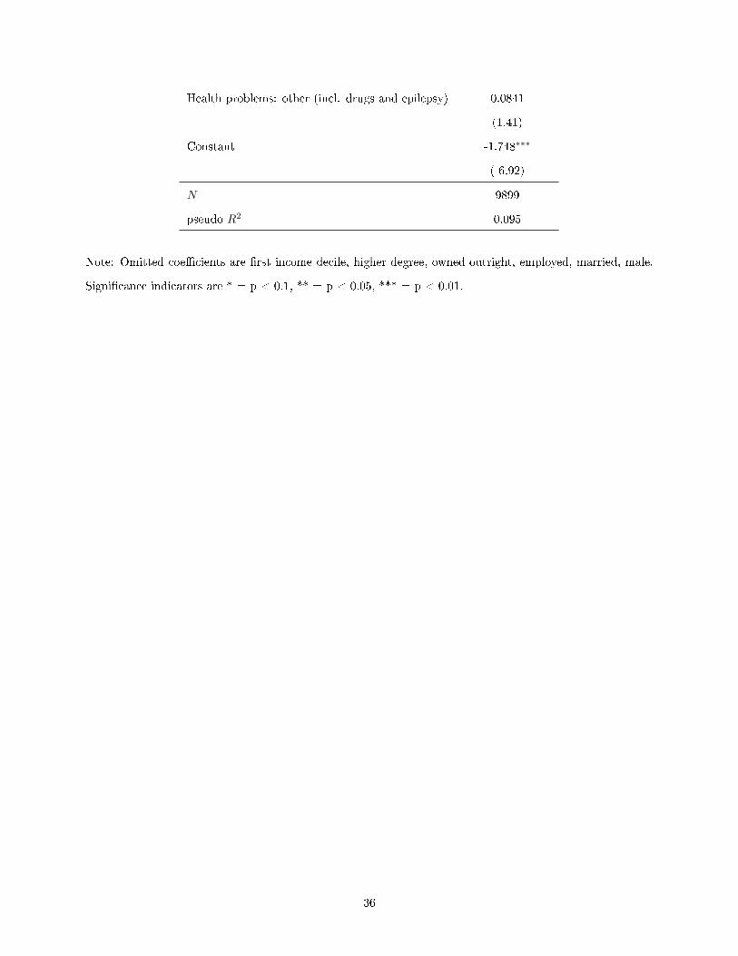
Health problems: other (incl. drugs and epilepsy) 0.0841

(1.41)

Constant -1.748∗∗∗

(-6.92)

N 9899

pseudo R2 0.095

Note: Omitted coe�cients are �rst income decile, higher degree, owned outright, employed, married, male.

Signi�cance indicators are * = p < 0.1, ** = p < 0.05, *** = p < 0.01.

36