anti-surge control - semantic scholar5. suggest tuning strategies for the various approaches....
TRANSCRIPT

June 2009Tor Arne Johansen, ITKBjørnar Bøhagen, ABB ASJørgen Spjøtvold, ABB AS
Master of Science in Engineering CyberneticsSubmission date:Supervisor:Co-supervisor:
Norwegian University of Science and TechnologyDepartment of Engineering Cybernetics
Anti-surge controlControl theoretic analysis of existing anti-surge control strategies
Terje Kvangardsnes


Problem Description1. Review various approaches for anti-surge control using a recycle valve.2. Establish simple dynamic model for analysis of control theoretic properties of thereviewed approaches in item 1. a. Neglect temperature dynamics and mole weight changes b. Include suction and discharge pressure dynamics c. Include compressor flow dynamics d. Include recycle line/valve flow dynamics3. Establish simulator for item 2 in Simulink and include typical industrial implementations.4. Analyze stability and performance of the various approaches found in item 1 using themodel in item 2, and verify using the simulator in item 3.5. Suggest tuning strategies for the various approaches.
Assignment given: 12. January 2009Supervisor: Tor Arne Johansen, ITK

Abstract
This report on compressor anti-surge control closes some of the gaps related tothe significant properties of control strategies. Anti-surge control is an impor-tant issue in operation of e.g. oil and gas processing plants. However, controlstrategies have not previously been studied thoroughly from a control theo-retic viewpoint. Special attention is given to the input-output relationship be-tween recycle valve opening and control variable when changing the compres-sor speed. The properties are then validated through simulations.
The compression system is found to be open-loop stable for operating pointsalong the surge control line. However, the behaviour of control variable in dif-ferent points is highly dependent on control strategy. A normalized control vari-able structure based on a operating point invariant to inlet conditions will per-form similarly for a range of compressor speeds. The report also provide greaterinsight in the dynamics of the compression system, along with guidelines forstrategy analysis and synthesis and controller tuning.


ix
Preface
This thesis is the culmination of 5 years spent at the Norwegian University ofScience and Technology (NTNU), studying for a MSc in Control Engineering.The problem description was given by ABB AS situated in Oslo, Norway.
Starting from scratch in January 2009, when considering insight in compres-sors and the field of compressor control, was a great challenge. There has beenboth frustrating and joyful moments during this journey. When it now all comesto an end, it is with great respect the results of my work is presented. The fieldof compressor control has a rich history, but hopefully some important aspectshave been pointed in this thesis.
There are many people who has played important roles while I was workingwith the thesis. First I would like to thank the fellow students and friends PerAaslid, Knut Ove Stenhagen, Eivind Lindeberg, Tore Brekke, Morten DinhoffPedersen and Lars Andreas Wennersberg. They have always been willing to dis-cuss matters of both technical and personal character, giving valuable feedback.
The cooperation with ABB has been fruitful and I would like to thank themand my supervisors at ABB Jørgen Spjøtvold and Bjørnar Bøhagen for fascilitat-ing my work and giving advice when needed.
Last but not least I would like to thank my family and friends for backing meup in though times, and especially my girlfriend for removing negative thoughtsand stress by a gentle touch.
I am now ready to embark the ship heading for my future, applying knowl-edge in other environments than the academic. Even though my status as astudent is cleared, I will always try to remember the words of Leonardo DaVinci:
“Learning never exhausts the mind.”
Terje Kvangardsnes Trondheim June 15th, 2009


xi
Contents
Abstract . . . . . . . . . . . . . . . . . . . . . . . . . . . . . . . . . . . iList of Figures . . . . . . . . . . . . . . . . . . . . . . . . . . . . . . . . xivList of Symbols . . . . . . . . . . . . . . . . . . . . . . . . . . . . . . . xvi
1 Introduction 11.1 Compressors . . . . . . . . . . . . . . . . . . . . . . . . . . . . . 11.2 Motivation . . . . . . . . . . . . . . . . . . . . . . . . . . . . . . . 21.3 Report organization . . . . . . . . . . . . . . . . . . . . . . . . . 2
2 Theory 32.1 Centrifugal compressor . . . . . . . . . . . . . . . . . . . . . . . . 3
2.1.1 Compressor maps . . . . . . . . . . . . . . . . . . . . . . . 42.1.2 Surge . . . . . . . . . . . . . . . . . . . . . . . . . . . . . 5
2.2 Compressor control . . . . . . . . . . . . . . . . . . . . . . . . . . 82.2.1 Surge control . . . . . . . . . . . . . . . . . . . . . . . . . 92.2.2 Surge avoidance with recycle valve . . . . . . . . . . . . . 10
2.3 Implementation issues . . . . . . . . . . . . . . . . . . . . . . . . 132.3.1 Invariance . . . . . . . . . . . . . . . . . . . . . . . . . . . 132.3.2 Surge control line . . . . . . . . . . . . . . . . . . . . . . 142.3.3 Flow measurement . . . . . . . . . . . . . . . . . . . . . . 152.3.4 Pressure measurements . . . . . . . . . . . . . . . . . . . 182.3.5 Control valve characteristics . . . . . . . . . . . . . . . . . 18
3 Modeling 213.1 Pressure dynamics . . . . . . . . . . . . . . . . . . . . . . . . . . 213.2 Duct flow . . . . . . . . . . . . . . . . . . . . . . . . . . . . . . . 223.3 Shaft dynamics . . . . . . . . . . . . . . . . . . . . . . . . . . . . 223.4 Compressor characteristics . . . . . . . . . . . . . . . . . . . . . . 233.5 Valve flow . . . . . . . . . . . . . . . . . . . . . . . . . . . . . . . 24
3.5.1 Check valve flow . . . . . . . . . . . . . . . . . . . . . . . 253.6 Compression system model . . . . . . . . . . . . . . . . . . . . . 253.7 Comments . . . . . . . . . . . . . . . . . . . . . . . . . . . . . . . 263.8 State space representation framework . . . . . . . . . . . . . . . 273.9 Equilibrium . . . . . . . . . . . . . . . . . . . . . . . . . . . . . . 28
xii
4 Analysis 314.1 Strategy analysis . . . . . . . . . . . . . . . . . . . . . . . . . . . 31
4.1.1 Surge control line . . . . . . . . . . . . . . . . . . . . . . 314.1.2 Control variable structure . . . . . . . . . . . . . . . . . . 314.1.3 Control variable dynamics . . . . . . . . . . . . . . . . . . 33
4.2 Strategy 1 . . . . . . . . . . . . . . . . . . . . . . . . . . . . . . . 374.2.1 Invariance . . . . . . . . . . . . . . . . . . . . . . . . . . . 374.2.2 Surge control line . . . . . . . . . . . . . . . . . . . . . . 374.2.3 Control variable structure . . . . . . . . . . . . . . . . . . 374.2.4 Control variable dynamics . . . . . . . . . . . . . . . . . . 39
4.3 Strategy 2 . . . . . . . . . . . . . . . . . . . . . . . . . . . . . . . 444.3.1 Invariance . . . . . . . . . . . . . . . . . . . . . . . . . . . 464.3.2 Surge control line . . . . . . . . . . . . . . . . . . . . . . 464.3.3 Control variable structure . . . . . . . . . . . . . . . . . . 474.3.4 Control variable dynamics . . . . . . . . . . . . . . . . . . 47
4.4 Summary . . . . . . . . . . . . . . . . . . . . . . . . . . . . . . . 51
5 Simulations 535.1 Strategy 1 . . . . . . . . . . . . . . . . . . . . . . . . . . . . . . . 53
5.1.1 System input pulse . . . . . . . . . . . . . . . . . . . . . . 535.1.2 Disturbance pulse . . . . . . . . . . . . . . . . . . . . . . . 55
5.2 Strategy 2 . . . . . . . . . . . . . . . . . . . . . . . . . . . . . . . 555.2.1 System input pulse . . . . . . . . . . . . . . . . . . . . . . 555.2.2 Disturbance pulse . . . . . . . . . . . . . . . . . . . . . . . 57
5.3 Summary . . . . . . . . . . . . . . . . . . . . . . . . . . . . . . . 58
6 Conclusion 616.1 Further work . . . . . . . . . . . . . . . . . . . . . . . . . . . . . 61
A Numerical values 67
B Linearization 69
C Transfer functions 71C.1 Strategy 1 . . . . . . . . . . . . . . . . . . . . . . . . . . . . . . . 71C.2 Strategy 2 . . . . . . . . . . . . . . . . . . . . . . . . . . . . . . . 73
D CD content 77

xiii
List of Figures
2.1 Compressor components . . . . . . . . . . . . . . . . . . . . . . . 42.2 Example of compressor map. . . . . . . . . . . . . . . . . . . . . 52.3 Surge cycle illustration . . . . . . . . . . . . . . . . . . . . . . . . 72.4 Compressor control approaches . . . . . . . . . . . . . . . . . . . 82.5 Fluid flow through orifice. . . . . . . . . . . . . . . . . . . . . . . 152.6 Non-corrected versus corrected mass flow ratio. . . . . . . . . . . 172.7 Non-corrected versus corrected mass flow ratio. . . . . . . . . . . 18
3.1 Compression system with recycle line. . . . . . . . . . . . . . . . 253.2 Changes in temperature versus changes in pressure. . . . . . . . . 273.3 Equilibrium of actuated system. . . . . . . . . . . . . . . . . . . . 29
4.1 Effect of SCL parameters. . . . . . . . . . . . . . . . . . . . . . . 32(a) b1 . . . . . . . . . . . . . . . . . . . . . . . . . . . . . . . . 32(b) b0 . . . . . . . . . . . . . . . . . . . . . . . . . . . . . . . . 32
4.2 Shortest distance. . . . . . . . . . . . . . . . . . . . . . . . . . . . 334.3 Interpretation of control variable. . . . . . . . . . . . . . . . . . . 384.4 Relative placement of zeroes and poles . . . . . . . . . . . . . . . 424.5 Movement of zeroes and poles . . . . . . . . . . . . . . . . . . . . 43
(a) 1,2,5 . . . . . . . . . . . . . . . . . . . . . . . . . . . . . . . 43(b) 3 . . . . . . . . . . . . . . . . . . . . . . . . . . . . . . . . . 43(c) 4,6 . . . . . . . . . . . . . . . . . . . . . . . . . . . . . . . . 43
4.6 3D bode plot. . . . . . . . . . . . . . . . . . . . . . . . . . . . . . 45(a) Amplitude . . . . . . . . . . . . . . . . . . . . . . . . . . . . 45(b) Phase . . . . . . . . . . . . . . . . . . . . . . . . . . . . . . 45
4.7 Normalized steady state gain for system input . . . . . . . . . . . 454.8 Normalized steady state gain for disturbances. . . . . . . . . . . . 46
(a) v1 . . . . . . . . . . . . . . . . . . . . . . . . . . . . . . . . 46(b) v2 . . . . . . . . . . . . . . . . . . . . . . . . . . . . . . . . 46
4.9 Interpretation of control variable. . . . . . . . . . . . . . . . . . . 474.10 Movement of zeroes and poles, corresponding value for lowest
Rp,e marked by a red downward pointing triangle. . . . . . . . . 50(a) 1,2,5 . . . . . . . . . . . . . . . . . . . . . . . . . . . . . . . 50(b) 3 . . . . . . . . . . . . . . . . . . . . . . . . . . . . . . . . . 50(c) 4,6 . . . . . . . . . . . . . . . . . . . . . . . . . . . . . . . . 50
4.11 Normalized steady state gain for system input . . . . . . . . . . . 51

xiv
4.12 Normalized steady state gain for disturbances. . . . . . . . . . . . 51(a) v1 . . . . . . . . . . . . . . . . . . . . . . . . . . . . . . . . 51(b) v2 . . . . . . . . . . . . . . . . . . . . . . . . . . . . . . . . 51
5.1 Strategy 1 control variable response to system input pulse . . . . 54(a) System input pulse . . . . . . . . . . . . . . . . . . . . . . . 54(b) Control variable response . . . . . . . . . . . . . . . . . . . 54
5.2 Strategy 1 control variable response to disturbance pulse . . . . . 56(a) Disturbance pulse . . . . . . . . . . . . . . . . . . . . . . . 56(b) Control variable response . . . . . . . . . . . . . . . . . . . 56
5.3 Strategy 2 control variable response to system input pulse . . . . 57(a) System input pulse . . . . . . . . . . . . . . . . . . . . . . . 57(b) Control variable response . . . . . . . . . . . . . . . . . . . 57
5.4 Strategy 2 control variable response to disturbance pulse . . . . . 58(a) Disturbance pulse . . . . . . . . . . . . . . . . . . . . . . . 58(b) Control variable response . . . . . . . . . . . . . . . . . . . 58
A.1 Curvefitted compressor map . . . . . . . . . . . . . . . . . . . . . 68

xv
List of Symbols
The following list explains the symbols used in the text, unless otherwise spec-ified. The meaning when used as subscript is marked (sub) and as a functionmarked (func).
Symbol Meaninga framework constantA cross sectional areab (func) surge control line parameterc constantc (sub) variable related to compressorc (func) surge control lineC Valve coefficientd (sub) outlet; also desired valued diameterD (func) transfer function denominatore (sub) equilibriume rotational speed errore (func) framework disturbancef (func) framework stateF forceg (func) framework inputh polytropic headh (func) framework measurementH (func) transfer functioni (func) framework control variable (measurement)j (func) surge lineJ inertiak ratio of specific heatk (func) framework control variable (states)K PID gains; also transfer function gainl recycle valve openingL length; also Lie derivative operator
xvi
m (sub) measured variablem massm (func) double derivative of control variableM molar massN rotational speed (rpm)N (func) transfer function numeratoro (sub) orificep pressureq volumetric flowr radiusr (sub) variable related to recycle flow; also corrected or reduced variableR with subscript denotes ratio; otherwise universal gas constants (sub) inlett (sub) variable related to check valveT temperatureu framework system inputv framework disturbance; also fluid flow velocityv (sub) property related to valveV volumew mass flowx framework statey framework measurementz framework control variableZ compressibilityα real part of complex numberβ imaginary part of complex numberρ densityσ polytropic compression exponentτ torqueΨ (func) compressor characteristicsψ (func) framework compressor characteristics

1
Chapter 1
Introduction
1.1 Compressors
The compressor is a mechanical device whose aim is to increase the pressureof a fluid. The term compressor is mostly used for for applications where thefluid is in gas state, whereas the term pump is used for increasing pressure inliquids.
How the pressure increase is achieved, depends on the type of compressor.Some increase pressure by reducing the volume occupied by the gas, e.g. recip-rocating compressors, scroll compressors and diaphragm compressors. Otherswork by first increasing fluid velocity, followed by a reduction of velocity to in-crease the fluid pressure due theory of energy conservation. If the fluid velocityis reduced without dissipating energy, kinetic energy will be transformed intopotential energy. Concerning gases, the increase in potential energy manifestsas both an increase in pressure and density.
Turbo compressors, hereunder axial and centrifugal/radial compressors, workby the latter principle. Energy is transferred to the fluid by a drive unit whichis connected to rotating blades called the impeller. This causes the fluid to ac-celerate, before it enters a stationary passage, the diffuser, where the fluid isdecelerated.
The terms axial and radial are related to which direction the fluid flowsthrough the impeller. The fluid flow in axial compressor is more or less parallellto the rotating axis of the compressor. For centrifugal compressors, fluid leavesthe impeller radially to the rotating axis.
Compressors are used in a wide range of applications. Axial compressorsare preferred where large flow rates or small physical dimensions are required.Centrifugal compressors on the other hand, are able to operate at higher pres-sures and are more resistant to erosive, dirty and corrosive gases. Examples ofapplications are:
• Gas transport
• Refrigerators and air conditioners
• Turbochargers for combustion engines
2 Chapter 1. Introduction
• Storage of air in containers e.g. for diving gear
Regardless of applications, turbo compressors may experience instabilityproblems related to their operating conditions. These instabilities are unwantedbecause they may lead to destruction of nearby equipment or the compressoritself, and can be avoided by ensuring that enough fluid flows through the com-pressor. One way of achieving minimum flow is to lead fluid from compressoroutlet to compressor inlet, or in other terms through fluid recycling. Recycleflow is regulated by a recycle valve. The state of the art protection schemesalso stabilize the compressor operation through active control of e.g. compres-sor rotational speed. However, in industrial application the simple, yet energyinefficient, recycling scheme is widely used to protect the compressor and itssurroundings.
1.2 Motivation
Even though the recycling scheme is old and the technology mature, there is alack of studies where control theoretic analysis tools have been used to studythe dynamics of the compression system including the recycle line. Further, asthe recycle valve opening often is determined by a simple PID controller withconstant gains, the linearity of control strategy is of importance. There are a va-riety of ways to synthesise the control variable used as input to the controller,and a few of these strategies will be analyzed in terms of its behaviour in dif-ferent compressor operating points.
1.3 Report organization
In chapter 2, theory related to the centrifugal compressor and its performanceis presented. Especially the instability phenomenon called surge is thoroughlydescribed. The chapter also contains a section presenting various compressorcontrol schemes and means to achieve control.
Chapter 3 presents a compression system model, and further adapts thismodel to a framework suited for control theoretic analysis. Some general con-siderations regarding the model properties and equilibria are also stated.
The analysis of the compression system and control strategies is given inchapter 4. First, the characteristics for different parts of a control strategyare identified, and general remarks concerning these characteristics presented.Then, two different control strategies are analyzed, both related to the pre-sented characteristics and their dynamic behaviour.
In chapter 5, simulations of the compression system models are performedto validate results from the control theoretic and structural analyses.
3
Chapter 2
Theory
The field of compressor control embrace a range of concepts which are essentialfor understanding the motivation behind different control strategies. The mostimportant of these concepts will be presented in the following chapter.
2.1 Centrifugal compressor
The compressor used further in this thesis is the centrifugal compressor, and amore detailed decription of its main characteristics follows. For further readingconsult e.g. [1].
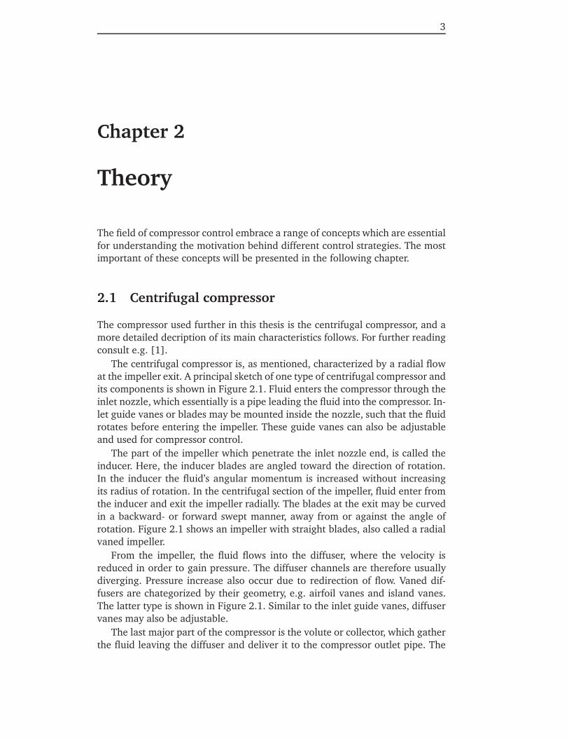
The centrifugal compressor is, as mentioned, characterized by a radial flowat the impeller exit. A principal sketch of one type of centrifugal compressor andits components is shown in Figure 2.1. Fluid enters the compressor through theinlet nozzle, which essentially is a pipe leading the fluid into the compressor. In-let guide vanes or blades may be mounted inside the nozzle, such that the fluidrotates before entering the impeller. These guide vanes can also be adjustableand used for compressor control.
The part of the impeller which penetrate the inlet nozzle end, is called theinducer. Here, the inducer blades are angled toward the direction of rotation.In the inducer the fluid’s angular momentum is increased without increasingits radius of rotation. In the centrifugal section of the impeller, fluid enter fromthe inducer and exit the impeller radially. The blades at the exit may be curvedin a backward- or forward swept manner, away from or against the angle ofrotation. Figure 2.1 shows an impeller with straight blades, also called a radialvaned impeller.
From the impeller, the fluid flows into the diffuser, where the velocity isreduced in order to gain pressure. The diffuser channels are therefore usuallydiverging. Pressure increase also occur due to redirection of flow. Vaned dif-fusers are chategorized by their geometry, e.g. airfoil vanes and island vanes.The latter type is shown in Figure 2.1. Similar to the inlet guide vanes, diffuservanes may also be adjustable.
The last major part of the compressor is the volute or collector, which gatherthe fluid leaving the diffuser and deliver it to the compressor outlet pipe. The
4 Chapter 2. Theory
AB
C
C
D
D
Figure 2.1: Compressor components shown from front and side where A: inducer B:impeller C: diffuser D: collector, and rotating parts are colored grey, andthe arrows indicate the direction of rotation.
collector, like the diffusor channels, have an increases in the cross sectional areasuch that fluid kinetic energy converts into pressure.
Centrifugal compressors may also have several stages, where two or moreimpellers are mounted on the same drive shaft. Fluid flows from one impeller tothe next via diffusors and collectors. Consequently, a series of single stage com-pressors constitute the multi stage compressor. A multi stage compressor is ableto produce the same pressure increase as that from a single stage compressorwith significantly larger impeller.
Compressors are often driven by electric motors or gas turbines. Electricdrive units are generally easier to control and have quicker response. However,for applications where use of electric power is impossible or undesireable, gasturbines may be employed as drive units. Especially natural gas compressorsare highly suitable for gas turbine drives, as the compression medium also fuelsthe compression system.
2.1.1 Compressor maps
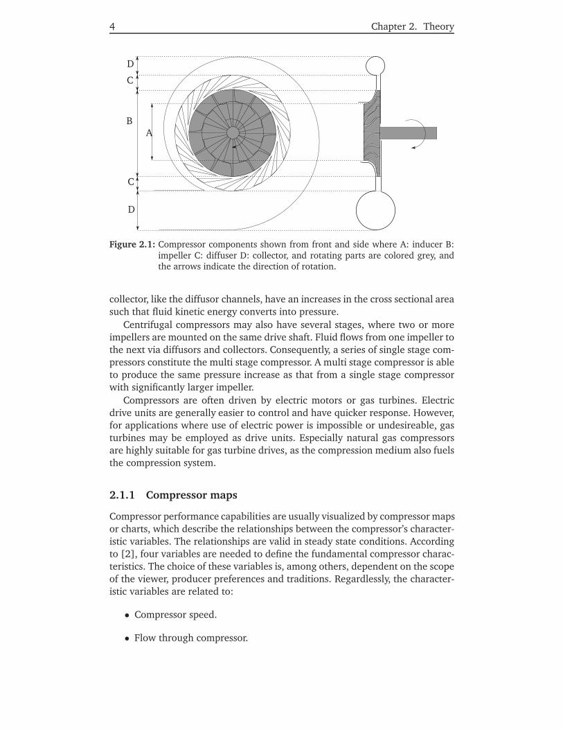
Compressor performance capabilities are usually visualized by compressor mapsor charts, which describe the relationships between the compressor’s character-istic variables. The relationships are valid in steady state conditions. Accordingto [2], four variables are needed to define the fundamental compressor charac-teristics. The choice of these variables is, among others, dependent on the scopeof the viewer, producer preferences and traditions. Regardlessly, the character-istic variables are related to:
• Compressor speed.
• Flow through compressor.
Chapter 2. Theory 5
Figure 2.2: Example of compressor map.
• Pressure rise 1.
• Energy efficiency.
An example compressor map is given in Figure 2.2, where the variable repre-senting energy efficiency is omitted.
2.1.2 Surge
Both axial and centrifugal compressor are subjected to different phenomenalimiting their operational range. The stonewall or choke phenomenon is char-acterized by fluid flowing through the compressor without any net increase inpressure, caused by a low load or discharge pressure. At this point, the flowresistance through the compressor equals the energy increase of the gas. Therotating stall phenomenon is in many ways the opposite, where fluid flow oscil-lates around zero with an increase in pressure. However, rotating stall is usu-ally referred to as local behaviour, only occuring in regions of the compressorwhile the net flow through the compressor is positive. But the most severe phe-nomenon when regarding compressor operational contraints is known as surge,characterized by oscillations in all of the compressor characteristic variables.
Rotating stall may develop such that flow oscillates in every part of the an-nular flow through the compressor. If no means are employed to counteract the
1By pressure rise is meant a general increase in pressure, not the special increase given by adifferential pressure Δp.

6 Chapter 2. Theory
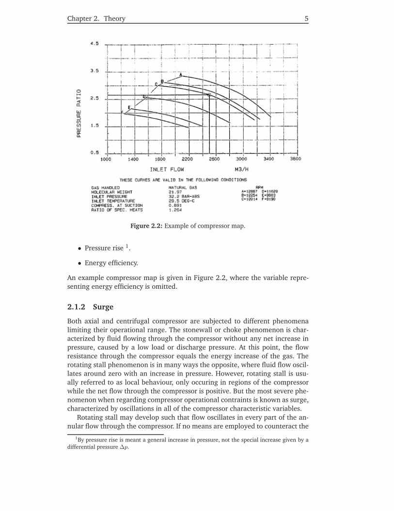
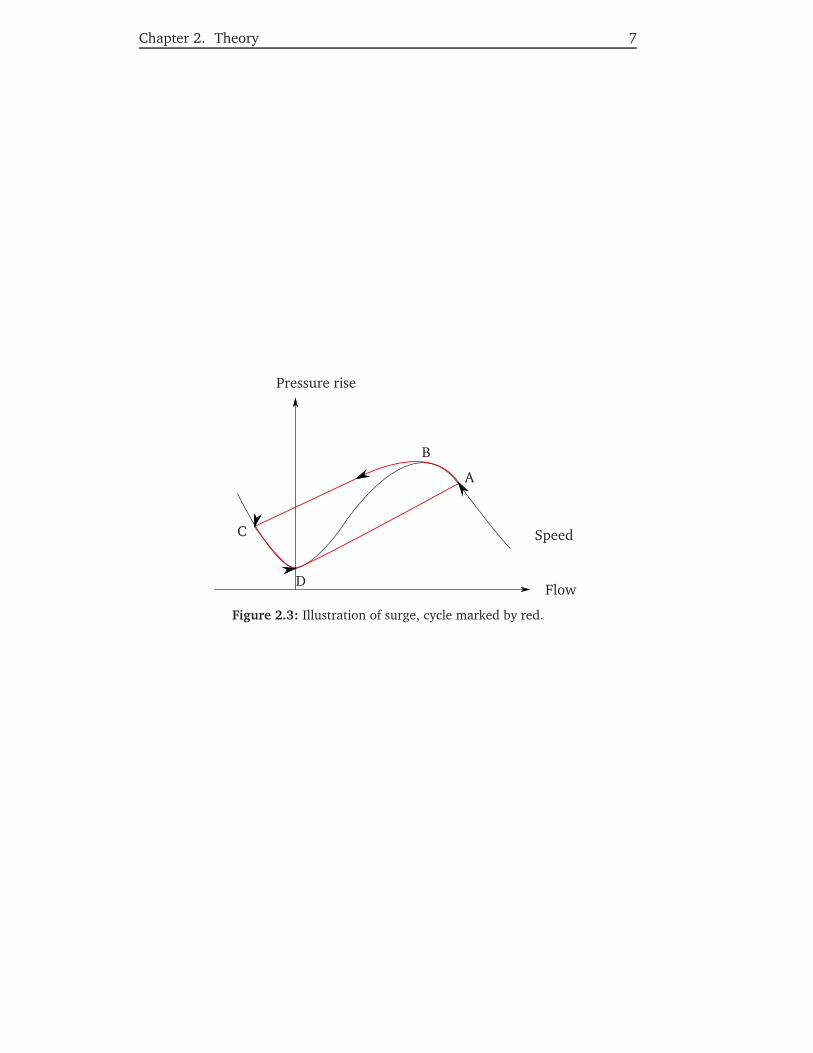
oscillations, the compressor will enter surge. Surge is more easily described onthe basis of an extended compressor map, see Figure 2.3. The stable operatingregion of the compressor lies to the right of point B in Figure 2.3, where pres-sure rise decreases for increasing flow. Also assume that the compressor speedis constant, implying that the operating point lie on the speed line shown in thefigure. The surge cycle can then be described by the following steps:
1. Assume that the compressor operates at point A, when the downstreampressure starts to increase. This causes compressor flow to decrease to thepoint where no further pressure rise through the compressor is possible,marked by B.
2. If the downstream pressure still exceeds the maximum pressure increase,flow will decrease and even become negative at point C. The negative flowcauses the upstream pressure to increase, and as a result the pressure riseover the compressor goes down.
3. At point D, the upstream pressure of the compressor is almost equal tothe downstream pressure. The compressor will then restore positive flow.
4. Flow will continue to increase until reaching point A. If no means areemployed to move out of the surge region, the surge cycle will repeat.
For a variable speed compressor, the stable and unstable regions of operationare separated by the surge line (SL). This line is usually determined by consid-ering the points on the compressor map where the pressure rise increase is zerofor increasing flow, which includes point B in 2.3.
The SL is usually independent of the energy efficiency, which is one of thevariables defining compressor characteristics. The remaining three variables arecoupled through the relations given by the compressor map. Consequently onlytwo variables are needed to describe the SL. But due to the non-linear com-pressor characteristics, the operating point of the compressor is not uniquelydetermined by every combination of these two variables, e.g. speed and pres-sure rise.
The surge phenomenon, unlike rotating stall, is a system instability whichaffects all states of the compression system. Speaking in terms of control theory,the surge cycle has the characteristics of a limit cycle.
Compressor surge may cause severe damage to the machinery and both up-stream and downstream components and is therefore highly undesireable. Var-ious means for preventing the occurance of surge or stabilizing the compressorwhen operating in the surge region will be presented later.
Chapter 2. Theory 7
Speed
Flow
Pressure rise
A
B
C
D
Figure 2.3: Illustration of surge, cycle marked by red.
8 Chapter 2. Theory
TV
RV
BV
CVIGV DV
SC
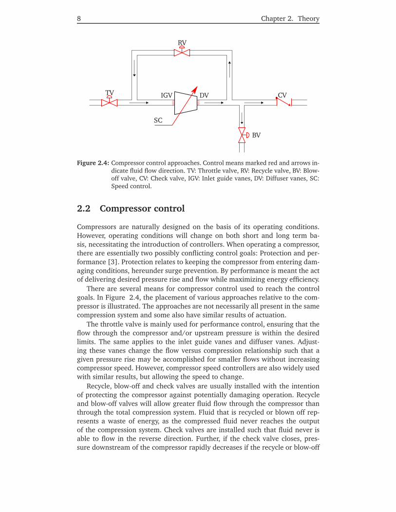
Figure 2.4: Compressor control approaches. Control means marked red and arrows in-dicate fluid flow direction. TV: Throttle valve, RV: Recycle valve, BV: Blow-off valve, CV: Check valve, IGV: Inlet guide vanes, DV: Diffuser vanes, SC:Speed control.
2.2 Compressor control
Compressors are naturally designed on the basis of its operating conditions.However, operating conditions will change on both short and long term ba-sis, necessitating the introduction of controllers. When operating a compressor,there are essentially two possibly conflicting control goals: Protection and per-formance [3]. Protection relates to keeping the compressor from entering dam-aging conditions, hereunder surge prevention. By performance is meant the actof delivering desired pressure rise and flow while maximizing energy efficiency.
There are several means for compressor control used to reach the controlgoals. In Figure 2.4, the placement of various approaches relative to the com-pressor is illustrated. The approaches are not necessarily all present in the samecompression system and some also have similar results of actuation.
The throttle valve is mainly used for performance control, ensuring that theflow through the compressor and/or upstream pressure is within the desiredlimits. The same applies to the inlet guide vanes and diffuser vanes. Adjust-ing these vanes change the flow versus compression relationship such that agiven pressure rise may be accomplished for smaller flows without increasingcompressor speed. However, compressor speed controllers are also widely usedwith similar results, but allowing the speed to change.
Recycle, blow-off and check valves are usually installed with the intentionof protecting the compressor against potentially damaging operation. Recycleand blow-off valves will allow greater fluid flow through the compressor thanthrough the total compression system. Fluid that is recycled or blown off rep-resents a waste of energy, as the compressed fluid never reaches the outputof the compression system. Check valves are installed such that fluid never isable to flow in the reverse direction. Further, if the check valve closes, pres-sure downstream of the compressor rapidly decreases if the recycle or blow-off
Chapter 2. Theory 9
valve opens, such that forward flow is quickly restored. Recycle valves are usu-ally installed where the gas itself is valuable, not only the pressure rise, such asnatural gas compression systems. Blow-off valves are used in air compressionapplications as air can be released directly into the atmosphere.
Even though the preceding means of control have been categorized by theirinitial reason for installment, they are also able to affect their opposing controlgoal. Speed control e.g. may be used to aid the recycle valve controller againstthe destructing effects of surge. Coordinated control have the potential to bothincrease compressor performance while ensuring safe operation.
2.2.1 Surge control
This section presents some of the most important control schemes developedfor surge control. The history of compressor surge control spans at least from1917 [4] to present. This rich past combined with the wide range of compressorapplications results in many different control schemes. Even though surge con-trol strategies have evolved from simple mechanical devices to state of the artcomputer based active surge control, insight in the development of compressorcontrol is of importance. The industry is conservative when considering newtechnology, especially for safety critical applications. Therefore, relatively oldcontrol schemes are still deployed in existing plants.
In general, technology specifications are protected by their owning company,which limits the possibility of obtaining direct knowledge from the developer.However, the same protective behavior results in patents open to the generalpublic. The literature reviewed in this survey is consequently to a large extentbased on filed patents. In addition to patents, articles on general compressordynamics and control are consulted with the aim of increased insight and un-derstanding.
Due to the vast number of patents only a selection of these can be reviewed.The selection represents the main trends and evolution of control schemes.The number of times that a patent has been cited by later patents and patentsassigned by main contributors in the field of compressor control, are believedto be of special importance. Existing control strategies can according to [5]and [2] be divided into three groups, characterized by their control goals. Thegroups are called surge avoidance, surge detection and avoidance, and activesurge control.
Surge avoidance has the aim of preventing surge by keeping the operatingpoint away from the surge region. Usually a static or dynamic surge controlline related to the surge lin is established, which increases the illegal regionof operation. This category is the main focus of this thesis and will be furtherexamined.
Surge detection and avoidance scheme inventors emphasize that some dis-turbances will cause the compressor operating point to enter the surge region,regardless of avoidance strategy. Further, surge avoidance schemes will effec-tively decrease the operating range of the compressor reducing its performance.Establishment of the surge line and corresponding surge control line requiresdetailed knowledge of the compressor’s geometry and construction, as well as
10 Chapter 2. Theory
operational values such as temperature, gas composition and pressure. Thesechallenges are not overcome by monitoring the operating point of the compres-sor, but by detecting incipient surge. Measurements reflecting characterisics ofincipient surge are converted into a surge control variable which is comparedto some threshold. When exceeded, means for recovering from the surge condi-tion are initiated. This eliminates the need for calculating the compressor oper-ating point and its distance to the surge line. Examples of patents are found in[6], [7] and [8]. This approach is fundametally different from surge avoidance,where surge is prevented prior to its occurance.
Active surge control is a relatively new discipline of compressor control,according to [2] first introduced in the literature by [9]. The goal of activesurge control is to extend the operating range of the compressor into the surgeregion by suppressing the effects caused by surge. The surge region can beregarded as open loop unstable. By introducing a controller, the compressorcan be stabilized also in the unstable region.
2.2.2 Surge avoidance with recycle valve
In [5] a comprehensive overview and discussion of different surge controlstrategies from its start to 1990 is presented. Surge avoidance schemes aregrouped into four categories. The categorization is based on how the threevariables suitable to describe proximity to surge are combined into a controlvariable.
• Category one is called “Conventional anti-surge control” and encompassstrategies where only flow and differential pressure across the compressorare measured. The control line is usually established by a static relation-ship between the measurements. The author describes some controllerstructures. A trend is that the inventions have special means for react-ing to rapid disturbances. Also, the controller tuning parameters are notstatic, but depend on the rate of approach or distance to the control line.
• Category two, “Flow/rotational speed”, the pressure rise of the compres-sor is neglected. Instead, the fluid flow is normalized by the compressorrotational speed to form a single variable which is compared to a set point.
• Category three, “Microprocessor and PLC 2 Based Controller”, is charac-terized by including measurements in addition to flow and pressure rise.Variables such as inlet temperature are measured to accurately calculatethe operating point and its location in the compressor map.
• Category four, “Control without flow measurements”, avoid the possiblyinaccurate and noisy flow measurement when computing the control vari-able. Pressure rise and compressor rotational speed or torque are the mostcommon measurements.
2Programmable Logic Controller.
Chapter 2. Theory 11
With the work done by [5] in mind, patents from the time after 1990 have beenexamined. The focus has been on the proposed controller structure, along withthe presented control variable.
In [10] a control scheme addressing the non-linear characteristics of thesurge line is proposed. A given change in pressure rise results in different re-sponse of the control system determined by placement of the operating pointin the compressor map. This is referred to as variable gain. As the control sys-tem performance is heavily influenced by the gain, it should be determined bythe system designer. The invention provides a system and device for balancingthe effects of variable gain, such that the total gain of the system is constantfor all operating points. The input to a PID controller is adjusted according tothe gradient of the non-linear surge control line at the operating point. A gainscheduling approach is also proposed, by calculating different gains for differ-ent operating points in advance. Including a discrete filter for the gain sched-uled values removes the discontiunous jumps which exist for gain scheduling.The standard flow rate and pressures upstream and downstream of the com-pressor are used to form the control variable, placing this invention in categoryone.
The standard PID controller may not be able to prevent surging if distur-bances are fast and/or flow rate is small. In [11], the inventor proposes anadditional controller which opens a quick acting solenoid valve when flow rateis below a static threshold. A selector chooses between the the signals fromthe standard PID controller and the fast response controller. Time dependentfunctions are used to ensure smooth transitions between the two controllersand provide extra safety margins when the quick emptying valve has been em-ployed.
A similar approach is proposed in [12]. The conventional PID controlleris used and the control variable belongs to in chategory one. To be able towithstand fast disturbances, an additional IPID controller is introduced. Thecontrol variable of the latter is the rate of change of the conventional PID’scontrol variable. According to the inventor, the additional integrator in the ratecontroller will cause the system to settle down even if the operating point isoutside the active region of the conventional PID controller. To allow higherfluctuations when operating far from the surge region, the setpoint of the ratecontroller is adjusted correspondingly.
In [13], the rate of approach to the surge line is counteracted by adjustingthe surge control line. First, a control variable which includes inlet and out-let temperatures, compression ratio and flow rate, and compressor rotationalspeed and guide vane position is calculated, a category three approach. Simul-taneously, the surge control line is established by adding to the surge line asteady state bias, an adaptive control bias determined from the time derivativeof the control variable, and a surge count bias based on the number of surgeevents experienced. The distance from the control variable to the surge con-trol line is input to a PI controller. The distance is also sent to an open-loopcontroller, which increments its control output if the distance is below a prede-termined threshold. Finally, the outputs from the two controllers are added andthe sum determine the anti surge valve opening.
12 Chapter 2. Theory
Another dynamic surge control line is applied in [14], on the basis of thecategory one variables flow rate and pressure rise. It is claimed that in the mostcommon control schemes, the valve is closed when operating to the right of thecontrol line, even if it approaches the surge region rapidly. The invention solvesthis by introducing a rate dependent bias on the surge control line, calculatedby the current distance to the set point substracted by a time delayed signal ofthe same distance. The time delay is large when the operating point approachesthe surge line, and small if it is directed away from the surge line.
An application note for compressor control by a specified controller is givenin [15]. The controller itself has a standard PID structure including integralanti-windup. But in addition, the closing rate is limited. This allows the PIDcontroller to be tuned for fast response, while at the same time avoiding thatthe valve is closed equally fast.
The invention in [16] comprises a control variable that is claimed to beindependent of molecular weight of the gas, compressor speed, temperatureand/or pressure. This way a single universal surge line can be plotted for alloperating conditions, and control is performed only by measuring flow, inletand outlet pressures, resulting in a category three scheme.
The scheme presented in [17] also pursues a control variable invariant ofoperating conditions, which especially adresses the the problems encounteredwhen the surge line is nearly horizontal. The basis of the control variable isthe one encountered in e.g. [13], but further manipulated into a new controlvariable.
Apparantly, most of the control schemes for surge avoidance with recyclevalves encountered in patent literature, incorporate a conventional PID con-troller. The contributions made by the patents can be divided into two groups:
• Improving response by adding more control structures
• Altering the control variables and measurements
Control under normal operating conditions is usually performed by the PIDcontroller, whereas the patents belonging to the first group tries to improve re-sponse when the system is subjected to rapid disturbances or emergency shut-down events (ESD). The patents in the second group aim to render the controlsystem invariant with respect to certain system variables and/or operating con-ditions.
Chapter 2. Theory 13
2.3 Implementation issues
When implementing anti surge control strategies, one has to take into accountpractical implementation aspects. Some of these aspects will be discussed inthe following section, with the aim to justify, describe and clarify existing antisurge strategies.
2.3.1 Invariance
Preferably, the operating point of the compressor should be given by variablesinvariant of the operating conditions of the compressor. Invariant variables de-scribes the distance to the surge limit in a uniform manner suited for anti-surgecontrol. If the compressor map were to be expressed by these invariant vari-ables, it would be fixed for all inlet conditions. An invariant compressor map isnaturally only valid for a specific compressor, but this limitation is due to thegeometry and construction of the compressor, not its operating conditions. Forthe discussion of anti-surge control, variables describing energy efficiency arenot important. Consequently, variables related to the latter characteristic willnot be presented.
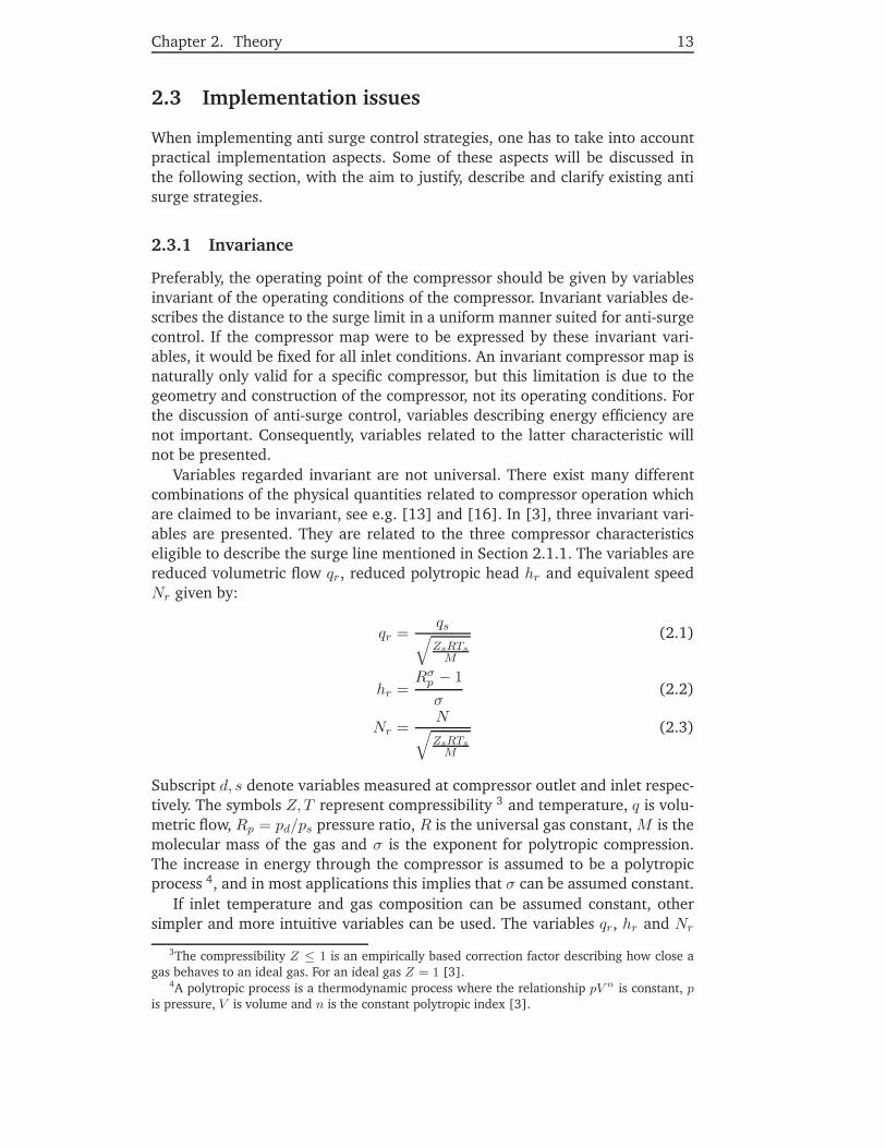
Variables regarded invariant are not universal. There exist many differentcombinations of the physical quantities related to compressor operation whichare claimed to be invariant, see e.g. [13] and [16]. In [3], three invariant vari-ables are presented. They are related to the three compressor characteristicseligible to describe the surge line mentioned in Section 2.1.1. The variables arereduced volumetric flow qr, reduced polytropic head hr and equivalent speedNr given by:
qr =qs√ZsRTsM
(2.1)
hr =Rσp − 1σ
(2.2)
Nr =N√ZsRTsM
(2.3)
Subscript d, s denote variables measured at compressor outlet and inlet respec-tively. The symbols Z, T represent compressibility 3 and temperature, q is volu-metric flow, Rp = pd/ps pressure ratio, R is the universal gas constant, M is themolecular mass of the gas and σ is the exponent for polytropic compression.The increase in energy through the compressor is assumed to be a polytropicprocess 4, and in most applications this implies that σ can be assumed constant.
If inlet temperature and gas composition can be assumed constant, othersimpler and more intuitive variables can be used. The variables qr, hr and Nr
3The compressibility Z ≤ 1 is an empirically based correction factor describing how close agas behaves to an ideal gas. For an ideal gas Z = 1 [3].
4A polytropic process is a thermodynamic process where the relationship pV n is constant, pis pressure, V is volume and n is the constant polytropic index [3].
14 Chapter 2. Theory
are then invertible functions 5 of q, Rp and N respectively. Consequently, thelatter variables may be assumed to be invariant.
For the remaining of this thesis, the volumetric flow on the SL is given as afunction of pressure ratio:
qSL
= j(Rp,SL) (2.4)
Even though the control variable should be invariant to varying inlet con-ditions, compressor maps are rarely given in terms of the previously presentedinvariant variables. Non-invariant compressor maps are only valid for given ref-erence operating conditions. However, because the compressor map, or morespecifically surge line, is the basis for developement of compressor controlstrategies, non-invariant variables should be corrected to fit the reference con-ditions. This correction is performed via the invariant variables.
If flow is represented by mass flow w, a correction factor can be found byconsidering flow at different conditions, relating them to volumetric flow andinserting ideal gas law (2.12):
wmρm
= q =wrρr
RTmpmM
wm =RTrefMpref
wr
wr =Tm/Trefpm/pref
wm (2.5)
Measured and corrected values are subscripted m and r respectively, while refdenote the reference condition given in the compressor map. For simplicity, itis assumed that the gas composition is equal to its reference, such that the gasmolar mass M can be eliminated.
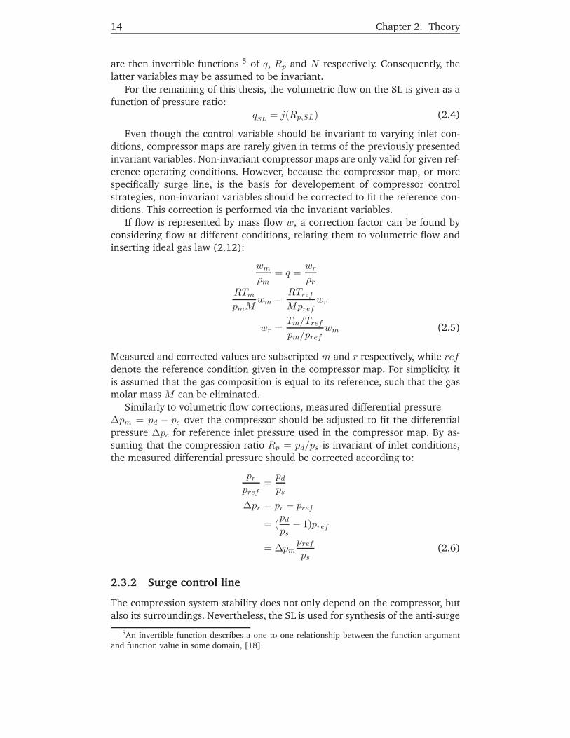
Similarly to volumetric flow corrections, measured differential pressureΔpm = pd − ps over the compressor should be adjusted to fit the differentialpressure Δpc for reference inlet pressure used in the compressor map. By as-suming that the compression ratio Rp = pd/ps is invariant of inlet conditions,the measured differential pressure should be corrected according to:
prpref
=pdps
Δpr = pr − pref
= (pdps
− 1)pref
= Δpmprefps
(2.6)
2.3.2 Surge control line
The compression system stability does not only depend on the compressor, butalso its surroundings. Nevertheless, the SL is used for synthesis of the anti-surge
5An invertible function describes a one to one relationship between the function argumentand function value in some domain, [18].
Chapter 2. Theory 15
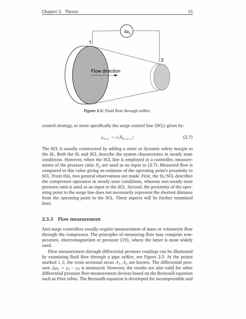
Figure 2.5: Fluid flow through orifice.
control strategy, or more specifically the surge control line (SCL) given by:
qSCL = c(Rp,SCL) (2.7)
The SCL is usually constructed by adding a static or dynamic safety margin tothe SL. Both the SL and SCL describe the system charateristics in steady stateconditions. However, when the SCL line is employed in a controller, measure-ments of the pressure ratio Rp are used as an input to (2.7). Measured flow iscompared to this value giving an estimate of the operating point’s proximity toSCL. From this, two general observations are made. First, the SL/SCL describesthe compressor operation in steady state conditions, whereas non-steady statepressure ratio is used as an input to the SCL. Second, the proximity of the oper-ating point to the surge line does not necessarily represent the shortest distancefrom the operating point to the SCL. These aspects will be further examinedlater.
2.3.3 Flow measurement
Anti-surge controllers usually require measurement of mass or volumetric flowthrough the compressor. The principles of measuring flow may comprise tem-perature, electromagnetism or pressure [19], where the latter is most widelyused.
Flow measurement through differential pressure readings can be illustratedby examining fluid flow through a pipe orifice, see Figure 2.5. At the pointsmarked 1, 2, the cross sectional areas A1, A2 are known. The differential pres-sure Δpo = p1 − p2 is measured. However, the results are also valid for otherdifferential pressure flow measurement devices based on the Bernoulli equationsuch as Pitot tubes. The Bernoulli equation is developed for incompressible and
16 Chapter 2. Theory
inviscid fluids 6 [20], essentially expressing conservation of energy for fluids.Assuming horizontal flow, the equation takes the form:
p1
ρ+v21
2=p2
ρ+v22
2(2.8)
where v1, v2 are flow velocities in point 1 and 2. The mass flow w is equalthrough the cross sections, assuming no mass accumulation. The pipe and ori-fice hole are assumed to have circular cross sections with diameters d1, d2:
w = ρA1v1 = ρA2v2 (2.9)
Combining (2.8) and (2.9), solving for mass flow, gives:
w = cd
√2ρΔpo1A2
2− 1
A21
= cdA2
√2ρΔpo1 − γ4
= cfA2
√2ρΔpo (2.10)
where cd is a coefficient included to correct for frictional losses and other mea-surement errors introduced by the geometry of the orifice, and γ is the ratio oforifice hole to pipe diameter d2/d1 < 1.
Gas expansion factor
The preceding result is based on the assumption that compression effects arenegligible for the differential pressure between points 1, 2. For gases, compres-sion effects may be included by multiplying (2.10) with the gas expansion fac-tor:
Y =
√√√√R2/ko
(k
k − 1
)(1 −R
(k−1)/ko
1 −Ro
)(1 − γ4
1 − γ4R2/ko
)(2.11)
where Ro = p2p1
and k = cpcv
is the specific heat ratio. For derivation of this factor,see [20].
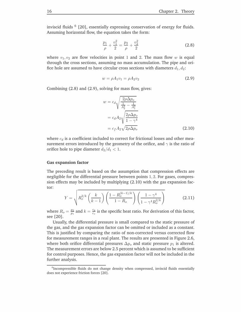
Usually, the differential pressure is small compared to the static pressure ofthe gas, and the gas expansion factor can be omitted or included as a constant.This is justified by comparing the ratio of non-corrected versus corrected flowfor measurement ranges in a real plant. The results are presented in Figure 2.6,where both orifice differential pressures Δpo and static pressure p1 is altered.The measurement errors are below 2.5 percent which is assumed to be sufficientfor control purposes. Hence, the gas expansion factor will not be included in thefurther analysis.
6Incompressible fluids do not change density when compressed, inviscid fluids essentiallydoes not experience friction forces [20].
Chapter 2. Theory 17
2.5
3
3.5
x 106
8
9
10
x 104
1.01
1.015
1.02
1.025
p1Δpo
Rat
io
Figure 2.6: Non-corrected versus corrected mass flow ratio.
Density variations
However, the assumption of incompressible fluid is not generally valid for gases.The density of the gas will vary with the static pressure, and consequently thiseffect should also be compensated for. The ideal gas law states that:
p = ρR
MT (2.12)
where R is the universal gas constant, M is the molar mass of the gas and Tis gas temperature as previously defined. Replacing ρ in (2.10) and assumingconstant temperature and gas composition gives:
w = cfA2
√2p1
M
RTΔpo = cw
√p1Δpo (2.13)
where cw = cfA2
√2MRT .
Volumetric flow can be computed from mass flow and orifice differentialpressure according to:
q =w
ρ= cqw
w
p1= cq
√Δpop1
(2.14)
where cq = cfA2
√2RTM and cqw = cq
cw= RT
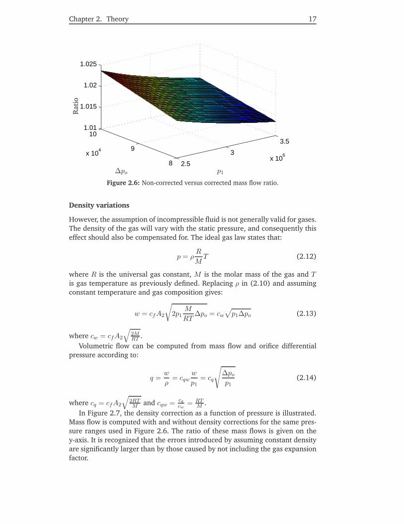
M .In Figure 2.7, the density correction as a function of pressure is illustrated.
Mass flow is computed with and without density corrections for the same pres-sure ranges used in Figure 2.6. The ratio of these mass flows is given on they-axis. It is recognized that the errors introduced by assuming constant densityare significantly larger than by those caused by not including the gas expansionfactor.

18 Chapter 2. Theory
2.5 3 3.5
x 106
0.9
0.95
1
1.05
1.1
1.15
p1R
atio
Figure 2.7: Non-corrected versus corrected mass flow ratio.
2.3.4 Pressure measurements
Pressure measurements are not nearly as complicated as flow measurements.Many principles of pressure measurements exist, each with different error sourcesand dynamic behaviour [19]. However, the error sources are not as closely re-lated to the system states as for flow measurements. For simplicity, pressuremeasurements are assumed to be perfect in the remaining of this thesis.
2.3.5 Control valve characteristics
Flow in the compression system is usually controlled by inserting valves in pipesand ducts. The steady state flow through a valve can be modeled by [21, page35]:
wv = C∗v (l)
√2ρΔp (2.15)
where wv is the mass flow through the valve, C∗v (l) is the valve flow coefficient,
l ∈ [0, 1] is the valve opening, ρ is the upstream density of the fluid and Δp =p1 − p2 is the pressure drop across the valve.
The flow coefficient C∗v is calculated in steady state conditions, at a certain
opening position and where Δp = 1Pa. The term valve characteristics is usedto describe how the flow coefficient varies as a function of opening position.There are three common valve characteristics:
• Linear C∗v = C∗
v,maxl.
• Quick opening C∗v = C∗
v,maxl1/μ, μ > 1.
• Equal percentage C∗v = C∗
v,maxφl−1, φ ≈ 50
Valves with linear and equal percentage characteristics are mainly used for con-trol purposes, whereas quick opening valves are ideal for applications wherelarge flow rates should be delivered as quickly as possible.
The recycle valve opening is regulated by a positioner, whose set point isgiven by the anti-surge controller. Consequently, the resulting recycle flow froma commanded valve opening will vary depending on the valve characteristics.

Chapter 2. Theory 19
As previously presented, anti-surge strategies are often based on standard linearPI(D) controllers with constant gains. However, the linear structure of the PIDcontroller will be distorted if employing valves with non linear characteristics.This may complicate controller tuning, as the valve response will be highlydependent on its opening.

21
Chapter 3
Modeling
The mathematical model used for analysis is based on the compression systemwith recycle valve model presented in [22, page 504], which again is basedon the famous Greitzer surge model from 1976. The model captures the maincharacteristics related to surge expressed by a set of differential equations. Pre-viously discussed phenomena apart from surge encountered in a compressionsystem, e.g. rotating stall, are not covered by the model. However, as the inher-ent goal of the anti surge controller is avoiding surge, other phenomena are oflimited interest. The model is developed by considering three principal models;pressure dynamics in a control volume, duct flow dynamics and shaft dynam-ics. The models presented will not be derived from their fundamental origin, forfurther insight the reader is adviced to consult e.g. [22] and other references.
3.1 Pressure dynamics
A gas compression system inludes a considerable amount of piping where fluidis able to accumulate. Further, in many gas compression systems the wet anddry parts of a fluid is separated in a component called a scrubber, ensuring thatno liquid enter the compressor. However, two phase flow 1 is out of scope ofthis thesis. By assuming that the amount of liquid accumulated in the scrubberis constant, the size of the volume occupied by gas will also be constant.
The presented pressure dynamic model may also be used to represent inter-connecting ducts, such that duct flow can be regarded one dimensional.
The pressure dynamics are derived by regarding a fixed control volume withuniform density. The rate of change of mass in the volume is described by:
V ρ = win −wout (3.1)
V is the control volume size, ρ is the density of the gas, win, wout are the massflows in and out of the volume. The relationship may be further refined byassuming that the gas in the volume is ideal, see Equation (2.12), and that the
1Two phase flow contain both liquids and gases [23].
22 Chapter 3. Modeling
thermodynamic behaviour of the gas can be regarded isentropic 2:
dp = c2i dρ (3.2)
where ci is the sonic velocity in the volume. The pressure differential equationfor a volume is then finally given by:
p =c2iV
(win − wout) (3.3)
3.2 Duct flow
Compression systems include, as mentioned, pipes or ducts in which fluid flowsbetween system components. The duct fluid flow also represent dynamic rela-tionships suitable to be expressed by differential equations. Flow can be mod-eled by considering the momentum equation of the fluid inside of the duct. Theduct is assumed to have constant cross sectional area A and connects two vol-umes with pressures p1 and p2. Further, fluid is assumed incompressible, onedimensional and with uniform axissymmetric velocity. The momentum equa-tion for the duct is then given by:
d
dt(mv) = Ap1 −Ap2 + F ′ (3.4)
where m = LAρ is the total fluid mass in the duct, v = wρA is the fluid velocity,
and F ′ describes the sum of all internal forces in the duct. L reflects the actualfluid flow path length which does not necessarily correspond to the physicallength of the duct.
Rewriting (3.4) gives a differential equation for the duct mass flow:
w =A
L(p1 − p2 + F ) (3.5)
where F = 1AF
′.
3.3 Shaft dynamics
Centrifugal compressors are large rotating systems, and the dynamics of theshaft will also affect the total compression system. The compressor may beactuated by different drives. However, the drive dynamics are not in the scopeof this thesis, hence drive torque is assumed to be delivered instantly. Shaftdynamics are modeled from conventional torque balance:
ω =1J
(τu − τl) (3.6)
where ω is the rotational speed of the compressor, J is the inertia of all rotatingparts in the compressor, τu is the drive torque, and τl is the load torque.
2A isentropic process resemble a polytropic process where pV n is constant, and no heat isremoved from or added to the gas [3].

Chapter 3. Modeling 23
The drive torque is assumed to be controlled by a conventional PID con-troller, whose aim is to keep the shaft rotational speed constant at ωd. The PIDcontroller is given by:
τu = Kpeω +Kdeω +Ki
∫e dt (3.7)
eω = ωd − ω (3.8)
The controller output is dependent on precise measurement of rotational speed.This measurement is assumed to be perfect, hence the rotational speed ω willbe directly used in the drive torque PID controller.
A simple load torque model is found in [22, page 488]. By assuming radialvanes in the impeller, the load torque is given by:
τl = r2wcω (3.9)
where r is the radius at the impeller outlet and wc is the compressor mass flow.
Error dynamics
To include the PID controller in the total compression system dynamics, theerror dynamics of the shaft and speed controller is derived. Differentiating (3.8)with respect to time, and inserting (3.6), (3.7) and (3.9) gives:
eω = −ω = − 1J
(Kpeω +Kdeω +Ki
∫eωdt − r2wc(ωd − eω))
= − 1Kd + J
(Kpeω +Ki
∫eωdt− r2wc(ωd − eω))
eω = − 1Kd + J
((Kp + r2wc)eω +Kieω − r2wc(ωd − eω))
(3.10)
3.4 Compressor characteristics
Compressor modeling is traditionally based on empirical studies of compressorsin steady state, which result in the previously described compressor map. Thecompressor map can also be derived by considering an isentropic process inseries with an isobaric process, for details consult [22]. In any case, the result-ing compressor characteristics must be related to the duct flow dynamics from(3.5). First, assume that the compressor characteristic is given by:
pdps
= Ψc(qc, ω) (3.11)
where pd, ps are pressures at the outlet and inlet of the compressor, and Ψc :RxR → R is the compressor map giving the pressure ratio of the compressor asa function of volumetric flow qc through the compressor and rotational speedω of the compressor shaft. The mapping from volumetric flow and rotationalspeed to pressure ratio implies that internal flow dynamics inside the compres-sor are fast compared to the overall compression system.

24 Chapter 3. Modeling
The duct mass flow (3.5) is in steady state condition given by:
p1 − p2 = Δp = −F (3.12)
In steady state, the pressure at the compressor inlet equals the pressure in theupstream volume, and the compressor outlet pressure equals the downstreamvolume pressure. Consequently, the compressor characteristic is related to thegeneral duct flow force by:
F = Ψc(qc, ω)p1 − p1
which inserted into (3.5) gives:
wc =AcLc
(Ψc(qc, ω)p1 − p2) (3.13)
representing the mass flow through the compressor in term of volume pres-sures upstream and downstream and the compressor map. The mass flow wcand volumetric flow qc are related, however the two notations are preservedto illustrate that the compressor map is expressed by invariant coordinates dis-cussed in Section 2.3.1.
3.5 Valve flow
The flow dynamics for ducts where valves are inserted are derived similarly tothe compressor flow, on basis of the equations given by (3.5) and (2.15).
By inserting the ideal gas law (2.12) into (2.15), the steady state flow canbe expressed for different upstream pressures:
wr = Cr(l)√p1Δp (3.14)
where Cr(l) = C∗v (l)
√2 MRT . Further, combining (3.14) and (3.12), gives:
F = − 1p1Cr(l)2
|wr|wr (3.15)
Finally, the dynamic behaviour of mass flow through the recycle line is givenby:
wr =AdLd
(p1 − p2 − 1p1Cr(l)2
|wr|wr) (3.16)
To avoid division by zero, l in Cr(l) is set to be in the range l ∈ [εl, 1], 0 <εl << 1. This implies that a small leakage flow through the valve occurs evenwhen fully closed. However, this implication will also be encountered in realapplications where the differential pressure over the valve is high [21].

Chapter 3. Modeling 25
Figure 3.1: Compression system with recycle line.
3.5.1 Check valve flow
Check valves only allow flow in one direction preventing reversed flow into thesystem. The ideal check valve has zero pressure loss, implying that F = 0 from(3.5). Consequently, the mass flow through the check valve is given by:
wt =AtLt
(p1 − p2)
wt > 0 (3.17)
3.6 Compression system model
The preceding component models are assembled into a complete model forthe compression system with recycle line, see 3.1. Pressure dynamics in thevolumes 1 and 2 denoted p1, p2 respectively, are described by (3.3). Volume 1represents the scrubber and piping upstream of the compressor, while volume2 is a relatively small volume downstream of the compressor inserted in theintersection of the compressor duct and the recycle line. Volume 3 is assumedto be so large that pa is constant.
Flow through the compressor wc is given by (3.13). The inlet and outletpressures of the duct where the compressor is mounted is given by the pressurein volume 1 and volume 2, respectively.
Further, recycle line flow wr is given by (3.16) where it is assumed thatpressure drop over the recycle valve equals pressure difference in volume 1 and2.
Check valve flow wt is governed by (3.17), whereas feed flow wf is consid-ered a system disturbance.
Finally, the compressor shaft dynamics are incorporated through the corre-sponding error dynamics from (3.8).

26 Chapter 3. Modeling
The total compression system model is then given by:
p1 =c21V1
(wf − wc + wr)
p2 =c22V2
(wc − wr − wt)
wc =AcLc
(Ψc(cqwwcp1, ω)p1 − p2)
wr =ArLr
(p2 − p1 − 1p2Cr(lr)2
|wr|wr)
wt =AtLt
(p2 − pa)
eω = − 1Kd + J
((Kp + r2wc)eω +Kieω − r2A
Lc(Ψc(wc, ω)p1 − p2)(ωd − eω))
(3.18)
The measurements in the system are given by the measurement vector y:
y =
⎡⎣ p1
p2
Δpo
⎤⎦ =
⎡⎢⎣p1
p2w2
cc2wp1
⎤⎥⎦ (3.19)
The pressures of volumes 1 and 2 are assumed to be measured directly, whereasthe flow through the compressor is measured by a flow element. The relation-ship between differential pressure across a flow element and mass flow is pre-sented in (2.13). Measurement of shaft rotational speed is not included in y, asthis is implicit in the speed error dynamics.
3.7 Comments
The model (3.18) does not include temperature dynamics. In many gas com-pression systems, temperature is regulated by heat exchangers to ensure highenergy efficiency in the compressor. Consequently, inlet temperature is assumedto be constant, density computed from ideal gas law Equation (2.12) is a func-tion of pressure only. This assumption can be justified by examining the ratio oftemperature measurements versus the mean temperature value, and the ratioof inlet pressure measurements versus the mean pressure value. Measurementsare taken from a real plant, and the ratios are presented Figure 3.2. It is recog-nized that pressure varies considerably more than temperature, hence densitychanges are mainly caused by pressure dynamics.
The temperature regulation violates the assumption of an isentropic processused in the derivation of the volume 1 pressure dynamics, as heat is removedfrom the system. However, recycle flow will partly compensate for the heat lossas the temperature of fluid on the compressor outlet usually is higher than thetemperature at the inlet.
The small volume 2 downstream of compressor may not meet the assump-tions regarding uniform density when check valve is closed. Inflow and outflow

Chapter 3. Modeling 27
Time step
Nor
mal
ized
tem
pera
ture
0 0.5 1 1.5 2 2.5 3 3.5×10⁴
0.9985
0.999
0.9995
1
1.0005
1.001
1.0015
1.002
1.0025
Figure 3.2: Changes in temperature versus changes in pressure.
regions of the volume where fluid velocity is non zero will affect density, andthe size of these regions are significant compared to the total volume. However,for positive throttle flow, volume 2 may be regarded as an integral part of largevolume 3. Hence, the model is more accurate when regarding positive throttleflow.
Regarding the recycle valve operation, no assumptions about the valve char-acteristics have been made. Hence, the system input u covers a wider range ofpossible implementations. The size of u will still be limited by the minimumand maximum values of the valve opening given by the assumptions for (3.15).
3.8 State space representation framework
The model (3.18) and strategies are transformed into a uniform state spaceframework for further analysis. The scope of this thesis lie on the different antisurge control strategies. Consequently, the compressor speed is assumed to beperfectly controlled and the error dynamics are neglected:
x = f(x) + g(x)1u
+ e(x)v
y = h(x)z = i(y)
(3.20)
where x denotes the system state space vector, u the scalar system input, v isdisturbance vector, y is the measurement vector, z the scalar control variableand f, g, e, h, i are vector functions. Finally, the system constants are gathered

28 Chapter 3. Modeling
in a vector a. The scalars, vectors and functions are defined by:
x =[p1 p2 wc wr wt
]Tu = Cr(lr)2
v =[wf pa
]Ta =
[c21V1
c22V2
AcLc
ArLr
AtLt
1c2w
cqw
]T(3.21)
f(x, u, a, v) =
⎡⎢⎢⎢⎢⎣
a1(−x3 + x4)a2(x3 − x4 − x5)a3(ψc(x3
x1)x1 − x2)
a4(x2 − x1)a5x2
⎤⎥⎥⎥⎥⎦
g(x) =[0 0 0 −a4
|x4|x4
x20]T
e(x) =[e1 e2
]=[a1 0 0 0 00 0 0 0 −a5
]T
h(x) =[x1 x2 a6
x23x1
]T
(3.22)
The function i(y) differ for the different anti surge control strategies, and istreated in later sections. Note also that the compressor map is represented byψc(x3
x1), assuming that the compressor speed is constant for the given timeframe.
3.9 Equilibrium
The equilibrium of the system when the recycle line is closed is determined byits boundary conditions or disturbances. The SCL can be viewed as a manifoldseparating the unactuated and actuated regions of compressor operation. If thedisturbances imply that the equilibria of the unactuated system lies to the leftof the SCL, the recycle valve must be opened to ensure safe operation of thecompressor. Assuming that the anti surge controller is able to drive the controlvariable to zero, the actuated system will have its equilibria on the SCL. Thiscan be stated as:
c(Rp,e) = qe (3.23)
where c(·) is the function from (2.7), and subscript e denotes the equilibrium.The shaft rotational speed of the compressor is assumed controlled. If the speedcontroller regulates speed according to a predetermined set point value ωd, theequilibrium of the actuated compression system will be explicitly determinedby the intersection of the corresponding speed line in the compressor map andthe SCL, see Figure 3.3.
The equilibrium for the whole compression recycle system can be found from(3.20), setting all derivatives to zero and assuming that the recycle valve must

Chapter 3. Modeling 29
ωd
q
Rp
SCL
Rp,e
qe
Figure 3.3: Equilibrium of actuated system.
be actuated to remain on the SCL by introducing the relationship from (3.23):
x1e =v2Rp,e
x2e = v2
x3e =v2qea7Rp,e
x4e =v2qea7Rp,e
− v1
x5e = v1
ue =( v2qea7Rp,e
− v1)2
v22(1 − 1/Rp,e)
(3.24)
The presented equilibria are valid for positive values of recycle flow, or:
c(Rp,e)Rp,e
>a7v1v2
(3.25)
which limits possible pressure ratio equilibria from below.
System input equilibrium
The equilibrium of the system input is dependent on the compression ratiowhere the SCL is defined. However, the latter observation does not imply thatthe largest system input on the surge line is given by the highest compressionratio. This can be explored by regarding the derivative of the equilibrium uewith respect to compression ratio Rp,e. If negative, this means that an increasein compressor speed will in fact require the recycle valve to be closed to remainon the SCL. Further, if the derivative equals zero:
∂ue∂Rp,e
= 0

30 Chapter 3. Modeling
will after some calculation imply that:
c(Rp,e)Rp,e
− a7v1v2
= 0 (3.26)
or
c(Rp,e)(2 − 1Rp,e
) + 2c′(Rp,e)(1 −Rp,e) − a7v1v2
= 0 (3.27)
where c′(Rp,e) = ∂c∂Rp
|Rp=Rp,e . The relationship in (3.26) describes the equi-librium with zero recycle flow which does not comply with the criterion from(3.25). However, if (3.27) is satisfied for a compression ratio in the compres-sor’s region of operation, the minimum and maximum valve openings will notnecessarily appear at the extremal values of compressor speed.
This previous aspects seem surprising, as an increase in speed means thatmore fluid should pass through the compressor to stay on the SCL. Assumingunchanged disturbances, the compressor flow increase must be a result of in-creased flow through the recycle line. However, the differential pressure acrossthe recycle valve will also be risen due to the speed change, such that the re-quired flow is achieved without further opening the recycle valve.
Example 3.1
Assume that the SCL is given by:
c(Rp) = c0√Rp − 1
Inserted into (3.26), will after some algebraic manipulation give:
R3p,e − (3 + (
a7v1v2c0
)2)R2p,e + 3Rp,e − 1 = 0 (3.28)
whose solutions are determined by the slope of the SCL and the size of the dis-turbances. The existence of solutions for positive values ofRp,e can be examinedby using the Descartes’ sign rule [24]. The rule states that the maxium numberof negative zeros for a polynomial P (x) can be found from counting the num-ber of sign changes in P (−x). Applied to (3.28), it is recognized that zero signchanges occurs. Consequently, all solutions of (3.28) are positive, showing thatpeaks in system input equilibrium may be encountered for feasible compressionratios.

31
Chapter 4
Analysis
This chapter first presents tools to categorize and analyse different anti surgestrategies and characteristics concerning the model (3.20), followed by a sec-tion where the tools are applied on presented strategies. Finally, simulationsemphasizing strategy characteristics are shown.
4.1 Strategy analysis
The different anti surge strategies will be assessed by their invariance accordingto those discussed in in 2.3.1. However, the strategies also differs in the struc-ture of the control variable and SCL. Some general properties of the dynamicsof the control variable when seen in relation to the whole compression systemwill also be presented.
4.1.1 Surge control line
The SCL is constructed by adding a safety margin to the SL. An expression forthe this way of constructing the SCL is given by:
c(Rp,SCL, t) = b1(Rp,SL
, t)j(Rp,SL) + b0(Rp,SL
, t) (4.1)
where b1 alters the slope of the SL, and b0 give an offset to the SL, see Figure4.1. Time varying SCL parameters are presented in e.g. [14] and [13] aiming todampen fast disturbances and avoid recurring surge events. The SCL may alsobe specified by a smooth function, e.g.:
c(Rp,SCL) = c0
√Rp,SCL
− 1 (4.2)
where it is ensured that the SCL lies to the right of the surge line for the wholeoperating region of the compressor.
4.1.2 Control variable structure
The control variable z describes the relation between a set point value qd(c(Rp))generated from the SCL and measured value q(q) generated from flow. Depend-ing on the sign of controller gains, z is positive or negative whenever qd > q. Inthe remaining of this thesis z > 0 if qd > q.

32 Chapter 4. Analysis
Speed lines
q
Rp
SCLSL
(a) b1
Speed lines
q
Rp
SCLSL
(b) b0
Figure 4.1: Effect of SCL parameters.
There are many ways to satisfy the latter criterion. Due to the linear struc-ture of the PID controller, the traditional synthesis of the variable z is a linearcombination of qd, q given by:
z1 = qd − q (4.3)
Another structure used in the industry is given by:
z2 = 1 − q
qd(4.4)
This normalization scheme cancels out terms which are common for both qdand q. However, it also implies that deviations from setpoint are expressed rel-ative to the set point value. This can be clarified by relating the two schemesaccording to:
z1 = z2qd (4.5)
Assuming that (4.4) determines the control variable, insertion of (4.5) into ageneral expression for a PID controller gives:
u =Kp
qdz1 +Kd
d
dt(z1qd
) +Ki
∫z1qd
dt (4.6)
The behaviour of this choice of control variable is not as transparent as thechoice of (4.3). If assuming a constant set point qd, it is clear that the controllergains are determined by the size of the set point.
Example 4.1
To illustrate the various aspects concerning the control variable and SCL, asimple example is presented. Assume that control variable is given by :
z = c(Rp)2 − q2
according to the structure in (4.3), and the SCL according to (4.2):
c(Rp) = c0√Rp − 1 (4.7)
Chapter 4. Analysis 33
R
q2
Rp
c(Rp)2 q2
d
z
SCL
Operating point
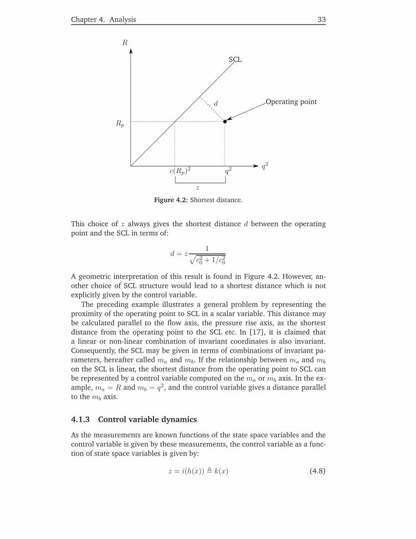
Figure 4.2: Shortest distance.
This choice of z always gives the shortest distance d between the operatingpoint and the SCL in terms of:
d = z1√
c20 + 1/c20
A geometric interpretation of this result is found in Figure 4.2. However, an-other choice of SCL structure would lead to a shortest distance which is notexplicitly given by the control variable.
The preceding example illustrates a general problem by representing theproximity of the operating point to SCL in a scalar variable. This distance maybe calculated parallel to the flow axis, the pressure rise axis, as the shortestdistance from the operating point to the SCL etc. In [17], it is claimed thata linear or non-linear combination of invariant coordinates is also invariant.Consequently, the SCL may be given in terms of combinations of invariant pa-rameters, hereafter called ma and mb. If the relationship between ma and mb
on the SCL is linear, the shortest distance from the operating point to SCL canbe represented by a control variable computed on the ma or mb axis. In the ex-ample, ma = R and mb = q2, and the control variable gives a distance parallelto the mb axis.
4.1.3 Control variable dynamics
As the measurements are known functions of the state space variables and thecontrol variable is given by these measurements, the control variable as a func-tion of state space variables is given by:
z = i(h(x)) � k(x) (4.8)
34 Chapter 4. Analysis
The time derivative of the control variable is:
z =∂k(x)∂x
x
=∂k(x)∂x
(f(x) + g(x)1u
+ e1v1 + e2v2)
= Lfk(x) + Lgk(x)1u
+ Le1k(x)v1 + Le2k(x)v2
= Lfk(x) + Le1k(x)v1 (4.9)
where Lfk(x) = ∂k(x)x f(x) is called the Lie derivative of k with respect to f. It is
recognized that the term Lgk(x) = 0, which means that the first time derivativeof the control variable is independent of system input u. This is clarified byrewriting Lgk(x):
Lgk(x) =∂k(x)∂x
g(x)
=∂i(h(x))∂x
g(x)
=∂i(y)∂y
∂h(x))∂x
g(x) (4.10)
where:∂h(x))∂x
g(x) =∂h(x1, x2, x3))
∂x
[0 0 0 −a4
|x4|x4
x20]T
= 0
The measurements are only dependent on states x1, x2, x3 while the systeminput appears in the differential equation describing x4. This is independent ofthe choice of control variable, as long as the current measurements are utilized.The same applies to Le2k(x).
The second time derivative of the control variable is, assuming constant dis-turbances:
z =∂[Lfk(x) + Le1k(x)v1]
∂xx
+∂[Lfk(x) + Le1k(x)v1]
∂xv
= L2fk(x) + LgLfk(x)
1u
+ Le1Lfk(x)v1 + Le2Lfk(x)v2
+ LfLe1k(x)v1 + LgLe1k(x)v11u
+ L2e1k(x)v
21 + Le2Le1k(x)v1v2
� m(x, u, v) (4.11)
Linearization
The system presented in (3.20), can be studied for small pertubations aroundan equilibrium through linearization [25, page 99]. The linearized system isgiven by:
Δx = AΔx+BΔu+EΔvΔz = CΔx (4.12)

Chapter 4. Analysis 35
where
A �∂(f(x) + g(x) 1
u + e(x)v)∂x
|e
B �∂(g(x) 1
u )∂u
|eE � e(x)|eC � ∂(k(x))
∂x
Δx � x− xe
Δu � u− ue
Δv � v − ve
The term |e denotes that the function is evaluated at the equilibrium given by(3.24). Matrices are given in appendix B.
One characteristic of a linear system, is that the frequency response frominput change to output change is independent of its operating point. This canbe shown by considering a general linear system:
x∗ = A∗x+B∗u∗ + E∗v∗
z∗ = C∗x∗
The linear system equilibrium is given by:
x∗e = (A∗)−1 [B∗u∗e + E∗v∗e ]z∗e = C∗x∗e
Hence, when the linear system dynamics are expressed by deviations from theequilibrium, we get:
Δx∗ = A∗Δx∗ +B∗Δu∗ + E∗Δv∗
Δz∗ = C∗Δx∗
The transfer functions are given by:
H∗u(s) =
N∗u(s)
D∗u(s)
= C∗ (sI −A∗)−1B∗ (4.13)
H∗v (s) =
N∗v (s)
D∗v(s)
= C∗ (sI −A∗)−1E∗ (4.14)
Consequently, the transfer functions (4.13) and (4.14) from control variableand disturbances, respectively, are independent of the operating point of thesystem.
This is not generally valid for a linearized system, as the matrices A,B,C,Eare dependent on the equilibrium. However, a non-linear system’s linearity maybe examined by regarding the transfer function of the linearized system in dif-ferent equilibria. Specifically, by calculating the eigenvalues and zeroes of the
36 Chapter 4. Analysis
linearized system, the main governing dynamics may be identified. How theseeigenvalues and zeroes are affected by changes in equilibrium, will give insightin the behaviour of the system in different equilibria. Further, for small frequen-cies the steady state gains given by Hu(0) and Hv(0) can be used to determinehow the system gain is affected by equilibrium changes.
Applied to the compression system, the equilibria of interest lie on the SCL.As previously mentioned, operating conditions which require an open recyclevalve to ensure safe operation of the compressor, give a system equilibrium onthe SCL. The SCL is parameterized in terms of the compression ratio Rp,e, butone should bear in mind that that an increase in steady state compression ratiocorresponds to increasing the compressor speed.
The size of the steady state gain is not interesting by itself, as the steady statedeviation caused by slow varying disturbances will be cancelled by the integraleffect in a controller. But for the purpose of controller tuning, it is necessary todetermine the area where the input to output gain is larger. If the input-outputgain increases significantly, a PID-controller with constant controller gains haveto be tuned such that the closed loop stability for high compression ratios ismaintained. However, a large gain difference might imply that the responseto a disturbance for low compression ratios is insufficient to avoid surge. Onthe other hand, if the input-output gain increase is small, the response to adisturbance for low compression ratios may be excessive such that oscillationsare induced.

Chapter 4. Analysis 37
4.2 Strategy 1
Control of the compression system is made on the basis of measured compressorpressure rise Δpc = p2 − p1 and differential pressure over an orifice Δpo,m.
4.2.1 Invariance
The differential pressure over the orifice representing compressor flow and inletpressure are combined according to:
q = Δpo,mKf
p1=q2cKf
c2q(4.15)
where Kf is an adjustment constant. Hence, the flow variable is proportionalto volumetric flow squared. As volumetric flow is regarded as an invariant vari-able, the same applies to the given flow variable. For simplicity, the relationshipKf/c
2q = 1 is used in the further analysis.
The differential pressure over the compressor is divided by inlet pressuregiving:
Δpp1
= Rp − 1 (4.16)
As previously discussed, pressure ratio can be regarded as an invariant variable.Consequently, the proposed pressure rise parameter is also invariant.
4.2.2 Surge control line
The surge control line is computed from the surge line by adding a margin inpercentage of flow, or:
c(Rp,SCL) = 1 + b1j(Rp,SL
) (4.17)
qd = c(Rp)2 (4.18)
4.2.3 Control variable structure
The control variable is computed from difference between qd and q in corre-spondance with (4.3):
z = c(Rp)2 − q2c (4.19)
The control variable can also be described by introducing the relation from(3.23), and describing the compressor flow in terms of volumetric flow qc:
z = c(Rp)2 − q2c
= c(Rp)2 − c(Rp,e)2 + q2e − q2c (4.20)
= (c(Rp) − c(Rp,e))(c(Rp) + c(Rp,e)) + (qe − qc)(qe + qc)= Δc(Rp)(Δc(Rp) + 2c(Rp,e)) + Δqc(2qe − Δqc)
= 2qe(Δc(Rp) + Δqc) + Δc(Rp)2 − Δq2c (4.21)
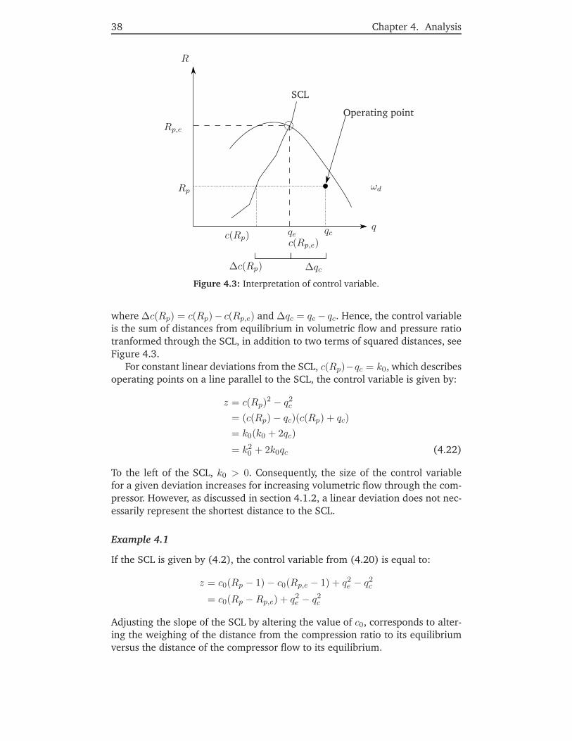
38 Chapter 4. Analysis
R
q
Rp,e
Rp
c(Rp) qec(Rp,e)
qc
Δc(Rp) Δqc
SCL
ωd
Operating point
Figure 4.3: Interpretation of control variable.
where Δc(Rp) = c(Rp)− c(Rp,e) and Δqc = qe− qc. Hence, the control variableis the sum of distances from equilibrium in volumetric flow and pressure ratiotranformed through the SCL, in addition to two terms of squared distances, seeFigure 4.3.
For constant linear deviations from the SCL, c(Rp)−qc = k0, which describesoperating points on a line parallel to the SCL, the control variable is given by:
z = c(Rp)2 − q2c
= (c(Rp) − qc)(c(Rp) + qc)= k0(k0 + 2qc)
= k20 + 2k0qc (4.22)
To the left of the SCL, k0 > 0. Consequently, the size of the control variablefor a given deviation increases for increasing volumetric flow through the com-pressor. However, as discussed in section 4.1.2, a linear deviation does not nec-essarily represent the shortest distance to the SCL.
Example 4.1
If the SCL is given by (4.2), the control variable from (4.20) is equal to:
z = c0(Rp − 1) − c0(Rp,e − 1) + q2e − q2c
= c0(Rp −Rp,e) + q2e − q2c
Adjusting the slope of the SCL by altering the value of c0, corresponds to alter-ing the weighing of the distance from the compression ratio to its equilibriumversus the distance of the compressor flow to its equilibrium.

Chapter 4. Analysis 39
4.2.4 Control variable dynamics
Adapted to the framework from (3.20), (4.19) is given by:
z = i(y) = c(y2
y1)2 −Kf
y3
y1
= c(x2
x1)2 − a7
x23
x21
= k(x) (4.23)
The compression ratio Rp = x2/x1 and the volumetric flow qc = a7x3/x1 arecoupled through the differential equations given in (3.20). We have:
qc = a7
(x3
x1− x3x1
x21
)
= a7
(x3
x1− qc
x1
a7x1
)
= a7
(x3
x1+ q2c
a1
a27
− qca1
a7(v1/x1 − x4/x1)
), (4.24)
x2
x1= ψc(
qca7
) − x3
a3x1(4.25)
Inserting the relationships from (4.24) and (4.25) into (4.23), leads to:
z = c(ψc(
qca7
) − 1a3a7
qc +a1
a3a27
q2c −a1
a3a7(v1/x1 − x4/x1)qc
)2− q2c (4.26)
This means that the control variable is dependent on volumetric flow and itsderivative. Used as an input to a PID-controller, it introduces damping effectseven if the derivative term of the controller is set to zero. Thus, even whenthe operating point of the compressor is to the right of the SCL, the valve willbe actuated for large fluctuations in flow. Numerous patents, e.q. [12], [13]and [14], has its main focus of improving response to high rates of approachto the SCL. It is pointed out that valve actuation when the operating point isto the right of the SCL, is undesireable. However, the definition of a SCL andusing pressure ratio measurements as its input, will implicitly include derivativeaction.
Example 4.2
The compressor map can be approximated in the vicinity of the equilibrium bya first order Taylor series expansion:
ψc(qca7
) ≈ ψc(qea7
) +1a7
(qc − qe)ψ′c(qea7
)
= Rp,e +1a7
(qc − qe)ψ′c(qea7
)
where ψ′c(qea7
) =∂ψc(
qca7
)
∂(qc/a7) |qc=qe < 0. Further, assume that the SCL is given by(4.7).

40 Chapter 4. Analysis
Inserted into (4.26), and introducing the relationship from (3.23), gives:
z = c20
(Rp,e +
1a7
(qc − qe)ψ′c(qea7
) − 1a3a7
qc +a1
a3a27
q2c −a1
a3a7(v1/x1 − x4/x1)qc − 1
)− q2c + q2e − c20(Rp,e − 1)
= − c20
a7ψ′c(qea7
)(qe − qc) − c20a3a7
qc − (1 − c20a1
a3a27
)q2c + q2e −c20a1
a3a7(v1/x1 − x4/x1)qc
≈ c20a7ψ′c(qea7
)(qc − qe) − c20a3a7
qc + q2e − q2c
where the terms v1/x1, x4/x1 and c20a1a3a27
are neglectable due to the physical lay-out of the compression system and its operating conditions. It recognized thatthe control variable is given by the deviation between the volumetric compres-sor flow and the equilibrium point and the time derivative of the same flow. Inother words, the difference between the SCL and flow variable, corresponds toa the flow variable’s distance to its equilibrium in addition to a damping effect.
Derivative
The second time derivative of the control variable is found from (4.11) and(4.23):
m(x, u, v) = L2fk(x) + LgLfk(x)u+ [Le1Lfk(x) + LfLe1k(x)]v1 + Le2Lfk(x)v2+ Le1
2k(x)v21 (4.27)
It can be recognized that LgLfk(x) �= 0. According to a term from [26, page510], the control variable z is said to have relative degree two with respect tothe system input u.
Transfer function
The transfer function Hu(s) is given in Appendix C. Even though there are alarge number of terms, some conclusions about the system can be made. It isseen that:
deg(Nu(s)) = 3 (4.28)
deg(Du(s)) = 5 (4.29)
The linearized system has relative degree deg(Du(s)) − deg(Nu(s)) = 2, whichcorresponds to the observation from (4.27). Further, as the degree of the de-nominator of the tranfer function equals the number of system states, there areno pole-zero cancellations for all equilibria on the SCL induced by the choice ofstrategy. According to [27, page 189], this implies that the system is observableand controllable, and there are no dynamic effects in the system which are notvisible through the control varible. However, there may be points on the SCLwhere the mentioned characteristics are not preserved.

Chapter 4. Analysis 41
The expression for steady state gain of the compression systemHu(0) = Nu(0)Du(0)
is given by:
Nu(0) = −2a72v2
2c (Rp,e)Rp,e2 (Rp,e − 1)2(a7 − ψ′
c(qea7
)c′(Rp,e))
(4.30)
Du(0) = (v2c (Rp,e) − v1a7Rp,e)[ψ′c
(qea7
)(v2c (Rp,e)
− 2v2Rp,ec (Rp,e) + v1a7Rp,e
)+ 2a7v2Rp,e(Rp,e − 1)
](4.31)
The negative sign illustrates that the control variable decreases when the re-cycle valve opening increases. The steady state gain size is of limited interest,however attention should be given to the its variations in different equilibria.
Due to the complexity of transfer function, insight is better acquired by re-garding a numerical example. The numerical values of the compression systemare presented in Appendix A.
Zeroes and poles
The relative positions of the zeroes and poles of the system in the complex planeis sketched in Figure 4.4. It includes references to Figure 4.5 where the move-ment of the poles and zeroes for increasing Rp,e is illustrated. The system hasthree distinct poles and one complex conjugate pole pair, one distinct zero andone pair of complex conjugate zeroes. All poles and zeros lie in the left half ofthe complex plane, except the complex conjugate zero pair. Hence, the systemis open loop stable and minimum phase. The transfer function can described interms of its zeroes and poles:
Hu(s) = K(s+ α5)(s− α6 + β6i)(s − α6 − β6i)
(s+ α1)(s+ α2)(s+ α3)(s+ α3 + β3i)(s + α3 + β3i)(s + α4)(4.32)
where K is the transfer function gain, and α,β denote the real and imaginaryparts of the zeroes and poles, respectively. In the following, the zeroes and polesare referenced by their subscript number.
First it is recognized that the pole 1, 2 and zero 5 shown in Figure 4.5(a) aresignificantly larger in absolute value than the other poles and zeros, hence thatparts of the system dynamics are much faster than others. By closer inspection,the size of pole 1 is found to be assosiated with the size of the system parametera3, which is related to the compressor duct dimensions. Increasing compressorduct length give slower response. The same arguments may be applied to pole2 and system parameter a4. Increasing recycle duct length will move pole 2 tothe right giving slower response. Depending on application and physical layoutof the compression system, some or all of these dynamics may very well beneglected, only employing their steady state solutions.
The complex conjugate pole pair denoted 3 lies to the right of pole 2 shownin Figure 4.5(b). A complex conjugate pole pair implies that there exist a res-onance frequency for the valve opening where the system output will oscillateheavily. Unlike the previously mentioned poles and zeros, the pair moves right

42 Chapter 4. Analysis
o x x x
x
x
o
oIm
Re
Figure 4.5(a)
Figure 4.5(b)
Figure 4.5(c)
Figure 4.4: Relative placement of zeroes and poles, poles marked by crosses and zeroesby circles.
for increasing pressure ratios/speed, such that a speed increase give less damp-ing and more rapid oscillations. Pole pair 3 is assosiated with parameter a5,causing the resonance frequency to be reduced if check valve duct length isincreased.
To the right of pole pair 3 in the complex plane, lies pole 4. In absolutevalue, this is the smallest of all poles and zeros. Consequently, the governingsystem dynamics are associated to pole 4. By increasing the value of volume 1,parameter a1 decreases, which again causes pole 4 to move to the right.
The complex conjugate zero pair 6 lies in the right half plane with a smallreal part, hence the linearized system is non minimum phase. In other words,slow opening of the recycle valve will move the control variable to negativevalues, but fast valve opening may cause the control variable to increase oroscillate even if the system states do not. According to [25], a non minimumphase system is harder to control because of the increased phase lag.
Due to the small real parts of pair 3 and 6 compared to their comples val-ues, the exponential behaviour of these dynamics are slow due to the lack ofdamping. It is also recognized that the imaginary part of these pairs increasefor increasing speeds, causing more oscillations for higher speeds.
All poles move strictly to the left when speed is increased, except pole pair 3which moves to the right. However, there are no crossing from left to right halfplane encountered in the numerical trials. Hence, most of the system dynamicsare faster when the compressor speed is increased and stability properties aremaintained.
Frequency analysis
To illustrate the effects caused by the poles and zeros in the previous section,three dimensional bode plot of the transfer function is presented in Figure 4.6.For low frequencies, the system phase is 180 ◦ due to the negative relation-ship between the system input and output, where an increase in valve openingcauses the control variable to decrease.
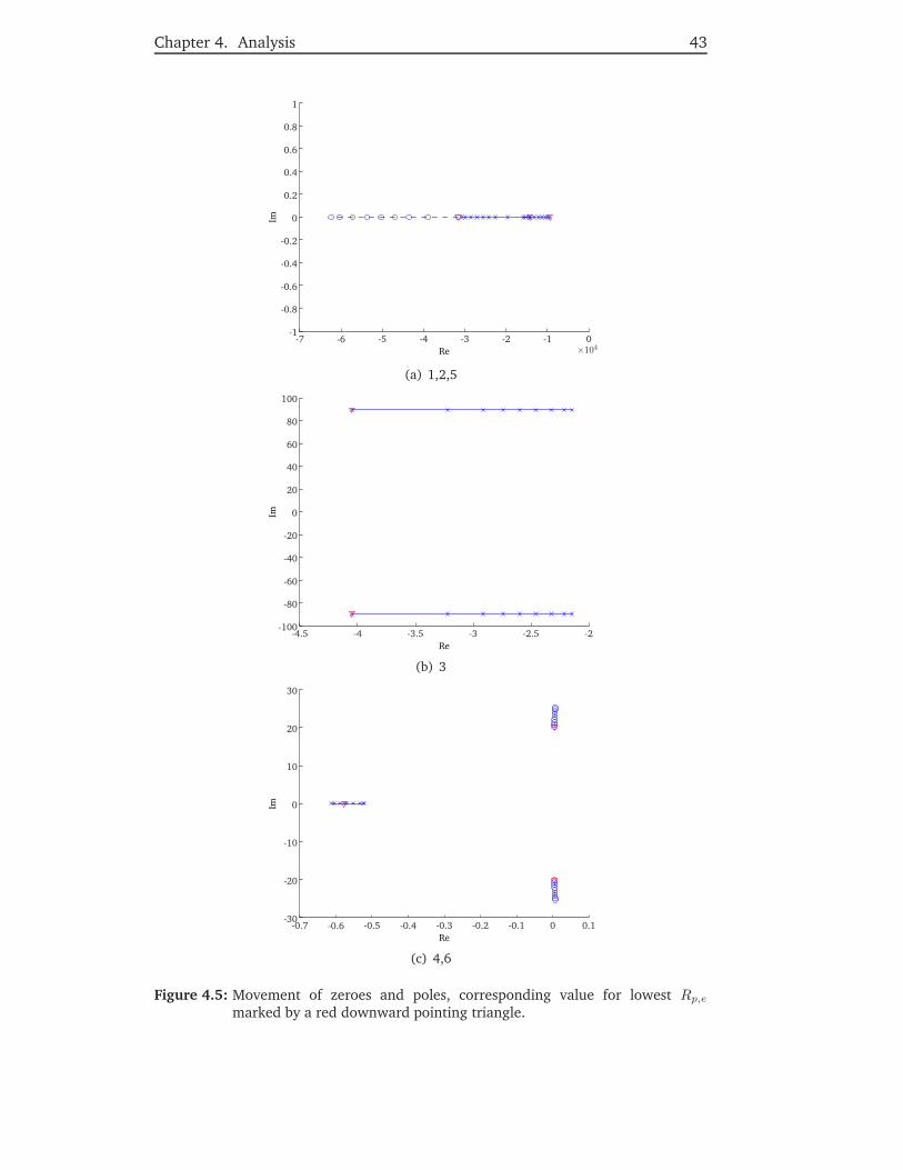
Chapter 4. Analysis 43
Re
Im
-7 -6 -5 -4 -3 -2 -1 0×104
-1
-0.8
-0.6
-0.4
-0.2
0
0.2
0.4
0.6
0.8
1
(a) 1,2,5
Re
Im
-4.5 -4 -3.5 -3 -2.5 -2-100
-80
-60
-40
-20
0
20
40
60
80
100
(b) 3
Re
Im
-0.7 -0.6 -0.5 -0.4 -0.3 -0.2 -0.1 0 0.1-30
-20
-10
0
10
20
30
(c) 4,6
Figure 4.5: Movement of zeroes and poles, corresponding value for lowest Rp,e
marked by a red downward pointing triangle.
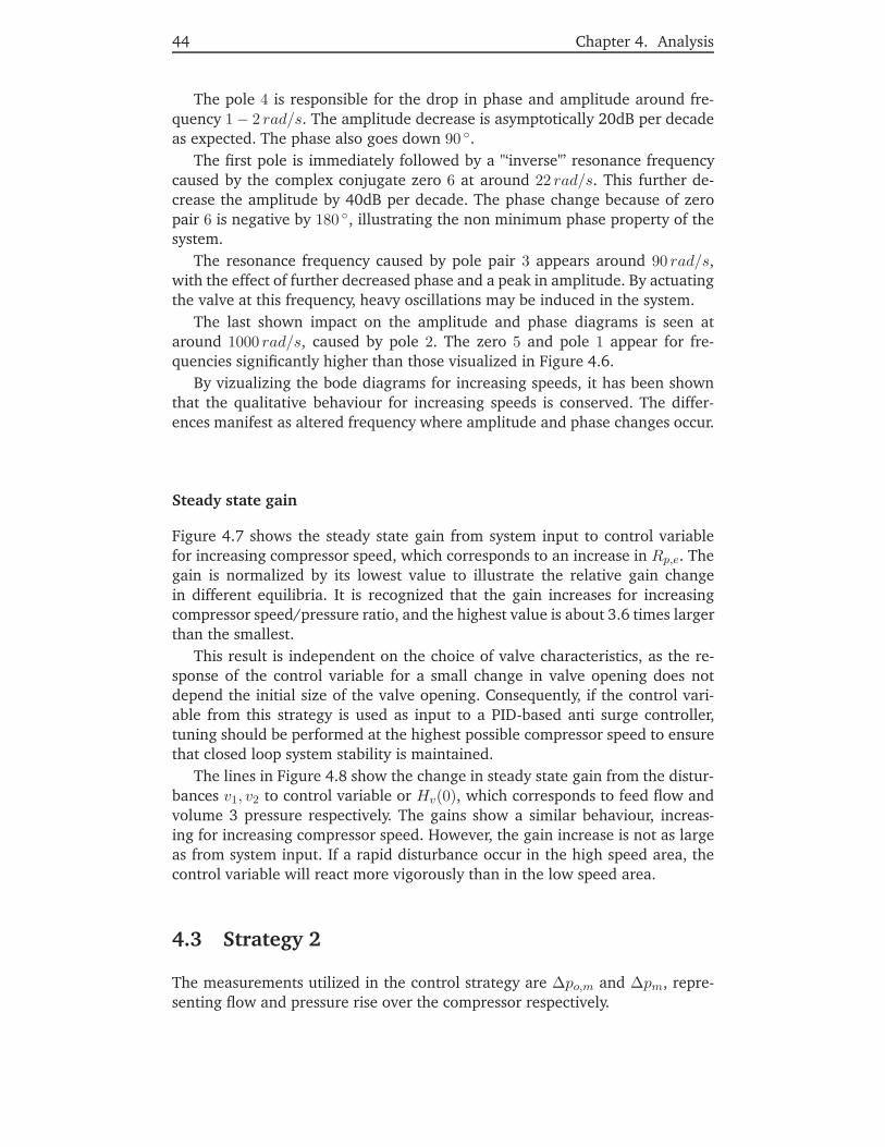
44 Chapter 4. Analysis
The pole 4 is responsible for the drop in phase and amplitude around fre-quency 1 − 2 rad/s. The amplitude decrease is asymptotically 20dB per decadeas expected. The phase also goes down 90 ◦.
The first pole is immediately followed by a "‘inverse"’ resonance frequencycaused by the complex conjugate zero 6 at around 22 rad/s. This further de-crease the amplitude by 40dB per decade. The phase change because of zeropair 6 is negative by 180 ◦, illustrating the non minimum phase property of thesystem.
The resonance frequency caused by pole pair 3 appears around 90 rad/s,with the effect of further decreased phase and a peak in amplitude. By actuatingthe valve at this frequency, heavy oscillations may be induced in the system.
The last shown impact on the amplitude and phase diagrams is seen ataround 1000 rad/s, caused by pole 2. The zero 5 and pole 1 appear for fre-quencies significantly higher than those visualized in Figure 4.6.
By vizualizing the bode diagrams for increasing speeds, it has been shownthat the qualitative behaviour for increasing speeds is conserved. The differ-ences manifest as altered frequency where amplitude and phase changes occur.
Steady state gain
Figure 4.7 shows the steady state gain from system input to control variablefor increasing compressor speed, which corresponds to an increase in Rp,e. Thegain is normalized by its lowest value to illustrate the relative gain changein different equilibria. It is recognized that the gain increases for increasingcompressor speed/pressure ratio, and the highest value is about 3.6 times largerthan the smallest.
This result is independent on the choice of valve characteristics, as the re-sponse of the control variable for a small change in valve opening does notdepend the initial size of the valve opening. Consequently, if the control vari-able from this strategy is used as input to a PID-based anti surge controller,tuning should be performed at the highest possible compressor speed to ensurethat closed loop system stability is maintained.
The lines in Figure 4.8 show the change in steady state gain from the distur-bances v1, v2 to control variable or Hv(0), which corresponds to feed flow andvolume 3 pressure respectively. The gains show a similar behaviour, increas-ing for increasing compressor speed. However, the gain increase is not as largeas from system input. If a rapid disturbance occur in the high speed area, thecontrol variable will react more vigorously than in the low speed area.
4.3 Strategy 2
The measurements utilized in the control strategy are Δpo,m and Δpm, repre-senting flow and pressure rise over the compressor respectively.

Chapter 4. Analysis 45
Speed
Frequency
Am
plit
ude
900
1000
1100
1200
1300
1400
10−5
100
105
104
106
108
1010
1012
(a) Amplitude
Speed
Frequency
Phas
e
900
1000
1100
1200
1300
1400
10−5
100
105
-400
-300
-200
-100
0
100
200
(b) Phase
Figure 4.6: 3D bode plot.
Speed
Ssga
in
950 1000 1050 1100 1150 1200 1250 1300 13501
1.5
2
2.5
3
3.5
4
Figure 4.7: Normalized steady state gain for system input over a range of compressorspeeds.
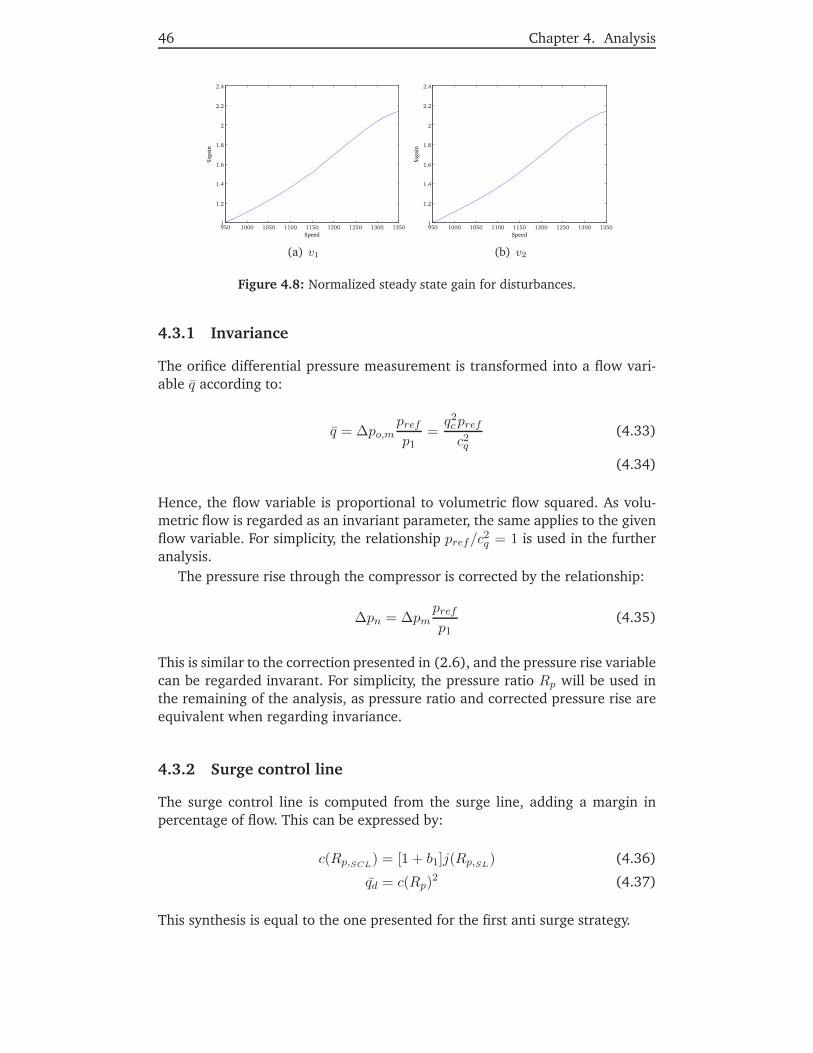
46 Chapter 4. Analysis
Speed
Ssga
in
950 1000 1050 1100 1150 1200 1250 1300 13501
1.2
1.4
1.6
1.8
2
2.2
2.4
(a) v1
Speed
Ssga
in
950 1000 1050 1100 1150 1200 1250 1300 13501
1.2
1.4
1.6
1.8
2
2.2
2.4
(b) v2
Figure 4.8: Normalized steady state gain for disturbances.
4.3.1 Invariance
The orifice differential pressure measurement is transformed into a flow vari-able q according to:
q = Δpo,mprefp1
=q2cprefc2q
(4.33)
(4.34)
Hence, the flow variable is proportional to volumetric flow squared. As volu-metric flow is regarded as an invariant parameter, the same applies to the givenflow variable. For simplicity, the relationship pref/c2q = 1 is used in the furtheranalysis.
The pressure rise through the compressor is corrected by the relationship:
Δpn = Δpmprefp1
(4.35)
This is similar to the correction presented in (2.6), and the pressure rise variablecan be regarded invarant. For simplicity, the pressure ratio Rp will be used inthe remaining of the analysis, as pressure ratio and corrected pressure rise areequivalent when regarding invariance.
4.3.2 Surge control line
The surge control line is computed from the surge line, adding a margin inpercentage of flow. This can be expressed by:
c(Rp,SCL) = [1 + b1]j(Rp,SL
) (4.36)
qd = c(Rp)2 (4.37)
This synthesis is equal to the one presented for the first anti surge strategy.
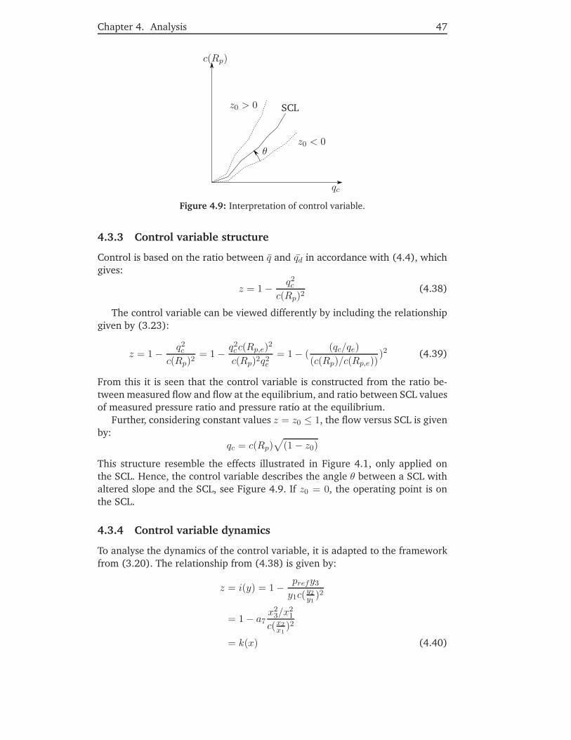
Chapter 4. Analysis 47
c(Rp)
qc
z0 > 0
z0 < 0θ
SCL
Figure 4.9: Interpretation of control variable.
4.3.3 Control variable structure
Control is based on the ratio between q and qd in accordance with (4.4), whichgives:
z = 1 − q2cc(Rp)2
(4.38)
The control variable can be viewed differently by including the relationshipgiven by (3.23):
z = 1 − q2cc(Rp)2
= 1 − q2cc(Rp,e)2
c(Rp)2q2e= 1 − (
(qc/qe)(c(Rp)/c(Rp,e))
)2 (4.39)
From this it is seen that the control variable is constructed from the ratio be-tween measured flow and flow at the equilibrium, and ratio between SCL valuesof measured pressure ratio and pressure ratio at the equilibrium.
Further, considering constant values z = z0 ≤ 1, the flow versus SCL is givenby:
qc = c(Rp)√
(1 − z0)
This structure resemble the effects illustrated in Figure 4.1, only applied onthe SCL. Hence, the control variable describes the angle θ between a SCL withaltered slope and the SCL, see Figure 4.9. If z0 = 0, the operating point is onthe SCL.
4.3.4 Control variable dynamics
To analyse the dynamics of the control variable, it is adapted to the frameworkfrom (3.20). The relationship from (4.38) is given by:
z = i(y) = 1 − prefy3
y1c(y2y1 )2
= 1 − a7x2
3/x21
c(x2x1
)2
= k(x) (4.40)

48 Chapter 4. Analysis
Further, including the dynamic coupling effects of the states from strategy 1given by (4.24) and (4.25) gives:
z = 1 − q2cc(ψc(
qca7
) − x3a3x1
)2
= 1 − q2c
c(ψc( qca7 ) − qca3a7
+ q2ca1a3a27
− qca1a3a7
(v1/x1 − x4/x1))2
(4.41)
The derivation of this result is identical to the one used in the analysis of thefirst strategy. The damping term introduced by qc appears in the denominatorof (4.41), but its effects are similar to the ones mentioned in the first analysis.Fast variations of compressor flow may cause the recycle valve to be actuated,even if the operating point is to the right of the SCL.
Derivative
The second time derivative of the control variable is:
m(x, u, v) = L2fk(x) + LgLfk(x)
1u
+ [Le1Lfk(x) + LfLe1k(x)]v1 + Le2Lfk(x)v2
+ Le12k(x)v2
1 (4.42)
The structure of (4.42) is equal to the one given by (4.27), but the terms arealtered. Nonetheless, the relative degree of two is preserved in this choice ofcontrol variable, which is expected as the same measurements are utilized inboth strategies.
Transfer function
The linearization procedure given by (4.12) is performed on the current strat-egy, and the resulting transfer function is presented in Appendix C. The obser-vations regarding the relative degree of the linearized system and the numberof poles are similar to the ones presented for the first strategy. This is expected,as the pole placement is a system property which is unaffected by the choice ofstrategy, and the same system input u and measurements y are used.
The steady state gain is given by:
Nu(0) = −2a72v2
2Rp,e2 (Rp,e − 1)2
(a7 − ψ′
c(qea7
)c′(Rp,e))
(4.43)
Du(0) = (v2c (Rp,e) − v1a7Rp,e) c (Rp,e)[ψ′c
(qea7
)(v2c (Rp,e)
− 2v2Rp,ec (Rp,e) + v1a7Rp,e
)+ 2a7v2Rp,e(Rp,e − 1)
](4.44)
The expression for the steady state gain is similar to the one given in (4.31). Infact, the only difference is the term c(Rp,e), which appears in the numerator of

Chapter 4. Analysis 49
strategy 1 and the denominator of strategy 2. Referring to the steady state gainfrom strategy 1 as Hu,1(0) and from strategy 2 as Hu,2(0), we have:
Hu,1(0)Hu,2(0)
= c(Rp,e)2 (4.45)
As the SCL described by c(Rp,e) is strictly increasing, the steady state gain fromstrategy 1 will be larger than strategy 2 when c(Rp,e) = qe > 1. However, asmentioned the size of the steady state gain is not interesting by itself, and thescaling difference from (4.45) will be counteracted by integral effects in thecontroller. The rest of the analysis will be conducted by numerical example,using the same parameters as for strategy 1.
Zeroes and poles
The system poles are independent of the proposed strategy. Consequently, thepole analysis for changing Rp,e presented in 4.2.4 also applies for strategy 2,and will not be repeated. The placement and behaviour of the zeroes are alsominimally affected by the change of control strategy, as seen in Figure 4.10.Consequently, the relative placement of the poles and zeros shown in 4.4 is stillvalid, along with the method of referring to poles and zero by their subscriptfrom (4.32).
Frequency analysis
Because the placement and movement of the zeros and poles are not signifi-cantly altered from strategy 1 to strategy 2, neither will the behaviour for in-creasing system input frequency shown in Figure 4.6. However, the figure doesnot illustrate very well the difference in gain encountered for increasing pres-sure ratios/speeds. For the latter analysis, the steady state gain of the systemwill give clearer indications.
Steady state gain
The steady state gain of strategy 2 is shown in Figure 4.11. Like for strategy 1,the gain strictly increases for increasing pressure ratios, which implies that tun-ing should be performed for high compression ratios/speeds. However, the gainincrease of 1.46 from lowest to highest value is significantly lower than strat-egy 1. Further, the Figures in 4.12 show the steady state gain change from thedisturbances to system output, where v1 is the inflow and v2 is the downstreampressure. It is recognized that the steady state gain actually strictly decreases forincreasing compressor speed, opposite of strategy 1. However the difference of1.16 is not large, such that a given change in disturbance will give almost equalchange in the control variable regardless of operating point of the compressionsystem.
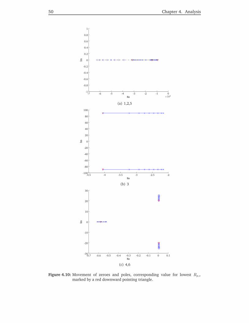
50 Chapter 4. Analysis
Re
Im
-7 -6 -5 -4 -3 -2 -1 0×104
-1
-0.8
-0.6
-0.4
-0.2
0
0.2
0.4
0.6
0.8
1
(a) 1,2,5
Re
Im
-4.5 -4 -3.5 -3 -2.5 -2-100
-80
-60
-40
-20
0
20
40
60
80
100
(b) 3
Re
Im
-0.7 -0.6 -0.5 -0.4 -0.3 -0.2 -0.1 0 0.1-30
-20
-10
0
10
20
30
(c) 4,6
Figure 4.10: Movement of zeroes and poles, corresponding value for lowest Rp,e
marked by a red downward pointing triangle.
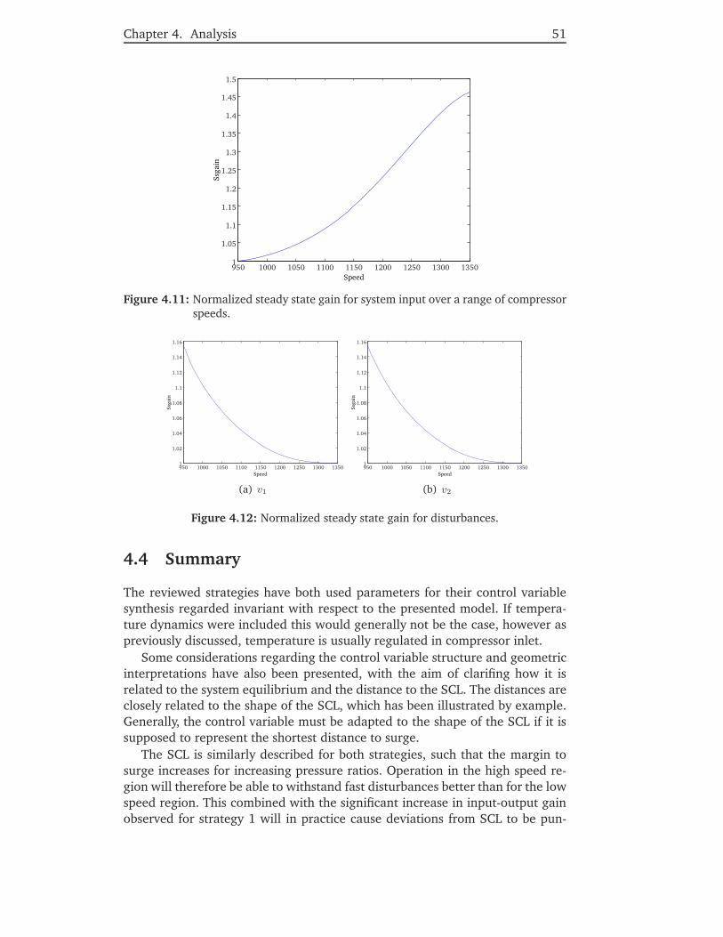
Chapter 4. Analysis 51
Speed
Ssga
in
950 1000 1050 1100 1150 1200 1250 1300 13501
1.05
1.1
1.15
1.2
1.25
1.3
1.35
1.4
1.45
1.5
Figure 4.11: Normalized steady state gain for system input over a range of compressorspeeds.
Speed
Ssga
in
950 1000 1050 1100 1150 1200 1250 1300 13501
1.02
1.04
1.06
1.08
1.1
1.12
1.14
1.16
(a) v1
Speed
Ssga
in
950 1000 1050 1100 1150 1200 1250 1300 13501
1.02
1.04
1.06
1.08
1.1
1.12
1.14
1.16
(b) v2
Figure 4.12: Normalized steady state gain for disturbances.
4.4 Summary
The reviewed strategies have both used parameters for their control variablesynthesis regarded invariant with respect to the presented model. If tempera-ture dynamics were included this would generally not be the case, however aspreviously discussed, temperature is usually regulated in compressor inlet.
Some considerations regarding the control variable structure and geometricinterpretations have also been presented, with the aim of clarifing how it isrelated to the system equilibrium and the distance to the SCL. The distances areclosely related to the shape of the SCL, which has been illustrated by example.Generally, the control variable must be adapted to the shape of the SCL if it issupposed to represent the shortest distance to surge.
The SCL is similarly described for both strategies, such that the margin tosurge increases for increasing pressure ratios. Operation in the high speed re-gion will therefore be able to withstand fast disturbances better than for the lowspeed region. This combined with the significant increase in input-output gainobserved for strategy 1 will in practice cause deviations from SCL to be pun-

52 Chapter 4. Analysis
ished harder than for strategy 2 in the high speed area. For lower speeds, thesmaller surge margin and input-output gain may be insufficient to withstandthe compressor operating point entering surge. Strategy 2 will have similar re-sponse for the presented speeds.
Qualitative dynamic behaviour is from the pole-zero and frequency analysisrecognized to be similar for both strategies. An increase in compressor speedimplies faster or more oscillatory dynamics for all states.
Flow and ratio control variable
From the expressions for the presented control variables given by (4.21) and(4.39), it is recognized that they both are constructed by a non linear mappingof the distance of the operating point to equilibrium. The contributions to thecontrol variable from flow distance and ratio distance is implicitly defined bythe SCL. It has also been shown that including measured compression ratio asinput to the SCL, have the effect of including additional damping in the controlsystem.
However, the SCL being responsible for the weighing of the flow distanceand ratio distance may not be the obvious choice. The SCL could rather repre-sent a safety margin only, such that tuning is decoupled from the definition ofthe SCL. A more flexible scheme for the control variable would e.g. be given by:
z = k1(ΔRp) + k2(Δqc) (4.46)
where ΔRp = Rp − Rp,e, Δqc = qe − qc. The functions k1(·) , k2(·) are possiblynon linear functions reflecting the operating points distance to the surge linefor the compression ratio and flow along the along the corresponding axes.This scheme assumes that the equilibrium is known which is valid if the desiredcompressor speed is made available. The equilibrium can then be calculated viathe SCL. On the downside, this would result in additional tuning parameters.

53
Chapter 5
Simulations
The model from (3.20) was implemented in MATLAB/Simulink R© to verifythe various system and strategy properties previously presented. The same pa-rameters used for the numerical analysis were employed, which are given inappendix A.
As shown in section 4.2.4, the compression system have parts of the dy-namics which are significantly faster than others. This is the characteristic of aso called stiff system [22], requiring other numerical solvers than system sim-ulations where the dynamics are less varying. The chosen algorithm was theode15s, a variable order solver suited for stiff systems. For further reading, seethe MATLAB Help file.
The time simulations have been performed by the following steps for a rangeof pressure ratios/compressor speeds:
1. Place the system state initial values in the equilibrium given by (3.24).This also means that the system input/valve opening differ for each speed.
2. Apply a pulse for one second on the input with a given percentage in-crease of the intial value.
3. Review response of control variable after pulse.
5.1 Strategy 1
5.1.1 System input pulse
The characteristic behaviour of the system for different speeds are shown inFigures 5.1. From Figure 5.1(a), it is first recognized that the valve openingstrictly decreases for increasing speeds. The demanded increase in recycle flowis more than satisfied by the higher pressure ratios, such that the valve mustbe closed to remain on the SCL. This also means that the system input pulseamplitude is lower for increasing speeds.
The qualitative behaviour of the control variable for increasing speed isidentical, which is seen from Figure 5.1(b). The behaviour can be character-ized as combination a first order response, and an underdamped second order

54 Chapter 5. Simulations
Time
Syst
emin
put
1000105011001150120012501300
10 10.5 11 11.5 12 12.5 13 13.5 14 14.5 151
1.2
1.4
1.6
1.8
2×10⁻¹²
(a) System input pulse
Time
Con
trol
vari
able
1000105011001150120012501300
10 10.5 11 11.5 12 12.5 13 13.5 14 14.5 15-20
-15
-10
-5
0
5×10⁻⁴
(b) Control variable response
Figure 5.1: Strategy 1 control variable response to pulse increase in system input oftwo percent. Colors represent the different compressor speeds.
response, where the second order dynamics are faster than the first order dy-namics. The oscillation frequency is by closer inspection found to be around90 rad/s. Further, it is seen that the response amplitude increases for increas-ing speed.
Referring to the zero and pole placement analysis in section 4.2.4, the contri-bution to the qualitative time response by poles 1, 2 and zero 5 are unobservabledue to the fast dynamics.
The first order response is therefore assosiated with pole 4, while oscilla-tions observed are caused by the pole pair 3. Pole 4 is smaller in absolute valuethan pair 3, such that dynamics related to pole 4 are slower than those relatedto pair 3. The pair 3 has a significantly larger imaginary than real part, imply-ing that oscillations will be poorly damped. The observed oscillation frequencyalso corresponds well with the resonance frequency of pole pair 3 of 90 rad/s.Consequently, the observed oscillations are caused by the check valve duct dy-

Chapter 5. Simulations 55
namics. The lack of damping terms in the modeling induces oscillations forrapid actuation of the recycle valve.
The increase in response amplitude of the control variable for increasingspeed was antisipated by the steady state gain analysis. Even though the systeminput pulse amplitude actually diminish, the gain increase overcompensates theamplitude reduction. The gain increase is related to the negative slope in com-pressor map. For the equilibria on the SCL, the slope becomes more negativefor increasing speeds. A small deviation from equilibrium will therefore cause amore vigorous response. The larger differential pressure for increasing speedswill also contribute to this behaviour.
5.1.2 Disturbance pulse
Simulations have also been performed where the disturbance feed flow hasbeen given an impulse while keeping system input/valve opening constant.The results of these simulations are given in Figure 5.2. Figure 5.2(a) showsthat the disturbance initial value and pulse is equal for all speeds, since the de-manded increase in compressor flow is maintained by the increased differentialpressure.
In Figure 5.2(b) it is seen that the asymptotic behaviour of the control vari-able is similar to the one caused by a pulse in system input. However, oscilla-tions are not observed. The amplitude of control variable is much larger thanresponse from the system input pulse, but in both cases there are increasingamplitude for increasing speed.
The large difference in amplitude for the disturbance pulse compared to thesystem input pulse are related to the amount the two pulsess inflict on totalcompressor flow. The recycle line flow is not only determined by valve opening,but also the differential pressure between volume 2 and volume 1. The feedflow on the other hand, is directly affected by the pulse.
The oscillations from the system input pulse does not appear, which is a con-sequence of where the pulse enter the system. The disturbance pulse initiallyaffect the dynamics associated with volume 1, previously identified as the slow-est dynamic component of the system. Therefore, all other system dynamics areable keep up with the changes inflicted on the volume 1 pressure, and fasterdynamics are not excited by the disturbance pulse.
As the amplitude of the response increases for increasing speed, the controlvariable will react more severly to a given disturbance when operating in thehigh speed area. This corresponds well with the conclusions from the steadystate gain analysis, and the response of the control variable to changes in systeminput.
5.2 Strategy 2
5.2.1 System input pulse
The previously described simulations where performed with the control vari-able from strategy 2, and the results are shown in Figure 5.3. The observations

56 Chapter 5. Simulations
Time
Dis
turb
ance
1000105011001150120012501300
10 10.5 11 11.5 12 12.5 13 13.5 14 14.5 157
7.2
7.4
7.6
7.8
(a) Disturbance pulse
Time
Con
trol
vari
able
1000105011001150120012501300
10 10.5 11 11.5 12 12.5 13 13.5 14 14.5 15-0.04
-0.03
-0.02
-0.01
0
0.01
(b) Control variable response
Figure 5.2: Strategy 1 control variable response to pulse increase in disturbance v1 often percent. Colors represent the different compressor speeds.
regarding the system input pulse are preserved from the strategy 1 analysis, asthe same scheme is used. This also applies to the qualitative behaviour of thecontrol variable for increasing speeds, and the relationships to the pole and zeroplacement. Hence, the observations and considerations presented for strategy1 will not be repeated.
However, there are significant differences regarding the amplitude of thecontrol variable response, and how this is affected by increasing speeds. Thesize of the amplitude is almost double of the one encountered in strategy 1.Further, the time response is almost equal for all compressor speeds.
The first obeservation implies that the overall gain from system input tocontrol variable is higher compared to strategy 1. When used as input to a con-troller, the controller parameters should therefore be smaller than if the controlvariable from strategy 1 was used and the same performance was desired. Thesecond observation regarding the small variations in time response for increas-ing speed is accordance with the result from the steady state gain analysis. In
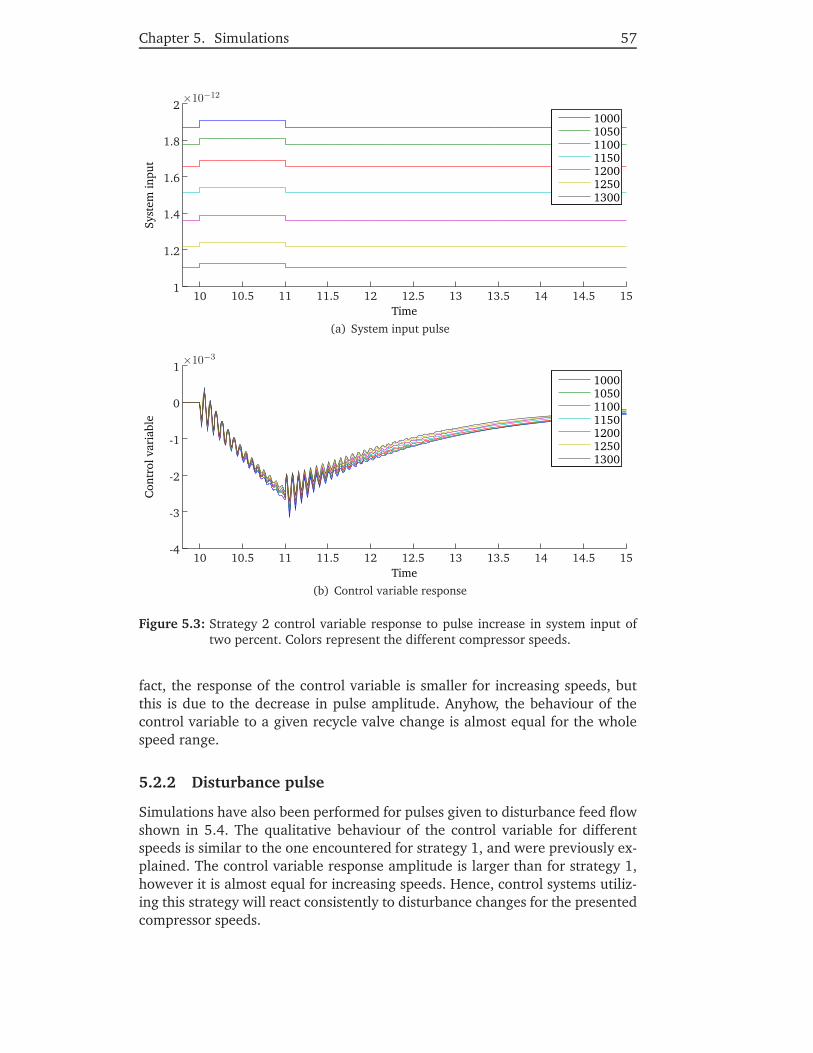
Chapter 5. Simulations 57
Time
Syst
emin
put
1000105011001150120012501300
10 10.5 11 11.5 12 12.5 13 13.5 14 14.5 151
1.2
1.4
1.6
1.8
2×10⁻¹²
(a) System input pulse
Time
Con
trol
vari
able
1000105011001150120012501300
10 10.5 11 11.5 12 12.5 13 13.5 14 14.5 15-4
-3
-2
-1
0
1×10⁻³
(b) Control variable response
Figure 5.3: Strategy 2 control variable response to pulse increase in system input oftwo percent. Colors represent the different compressor speeds.
fact, the response of the control variable is smaller for increasing speeds, butthis is due to the decrease in pulse amplitude. Anyhow, the behaviour of thecontrol variable to a given recycle valve change is almost equal for the wholespeed range.
5.2.2 Disturbance pulse
Simulations have also been performed for pulses given to disturbance feed flowshown in 5.4. The qualitative behaviour of the control variable for differentspeeds is similar to the one encountered for strategy 1, and were previously ex-plained. The control variable response amplitude is larger than for strategy 1,however it is almost equal for increasing speeds. Hence, control systems utiliz-ing this strategy will react consistently to disturbance changes for the presentedcompressor speeds.
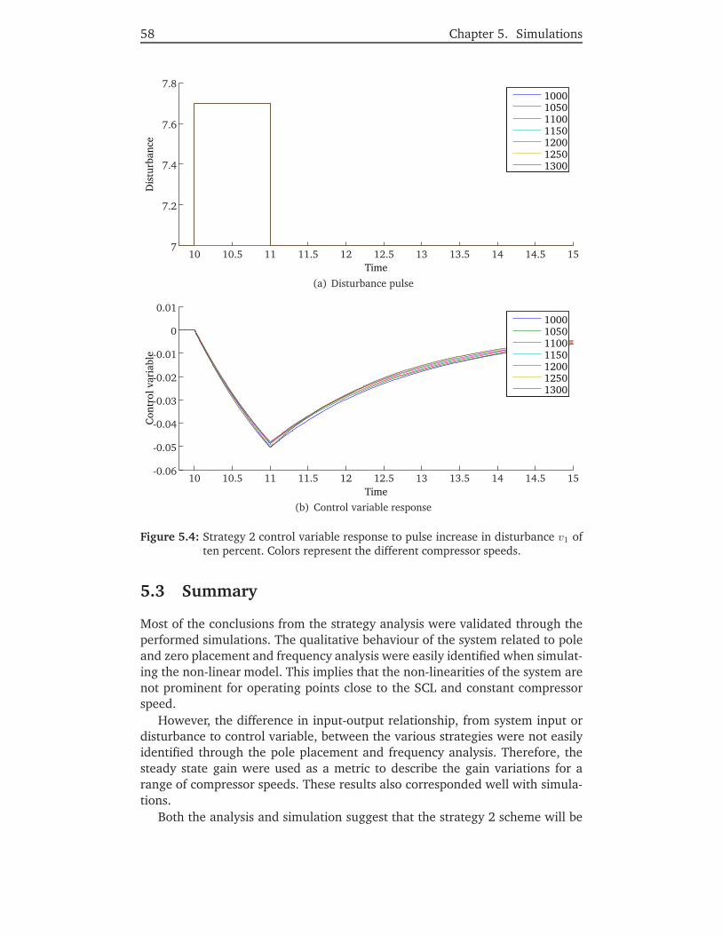
58 Chapter 5. Simulations
Time
Dis
turb
ance
1000105011001150120012501300
10 10.5 11 11.5 12 12.5 13 13.5 14 14.5 157
7.2
7.4
7.6
7.8
(a) Disturbance pulse
Time
Con
trol
vari
able
1000105011001150120012501300
10 10.5 11 11.5 12 12.5 13 13.5 14 14.5 15-0.06
-0.05
-0.04
-0.03
-0.02
-0.01
0
0.01
(b) Control variable response
Figure 5.4: Strategy 2 control variable response to pulse increase in disturbance v1 often percent. Colors represent the different compressor speeds.
5.3 Summary
Most of the conclusions from the strategy analysis were validated through theperformed simulations. The qualitative behaviour of the system related to poleand zero placement and frequency analysis were easily identified when simulat-ing the non-linear model. This implies that the non-linearities of the system arenot prominent for operating points close to the SCL and constant compressorspeed.
However, the difference in input-output relationship, from system input ordisturbance to control variable, between the various strategies were not easilyidentified through the pole placement and frequency analysis. Therefore, thesteady state gain were used as a metric to describe the gain variations for arange of compressor speeds. These results also corresponded well with simula-tions.
Both the analysis and simulation suggest that the strategy 2 scheme will be

Chapter 5. Simulations 59
less sensitive to speed changes, giving a more uniform response of the controlvariable, and that controller tuning should be performed for high compressorspeeds. Valves with other characteristics than the linear will have their greatestamount of change when the initial valve opening is small. Other system pa-rameters may give other results, but the main characteristics are believed to bemaintained as long as the parameters are kept within certain boundaries.

61
Chapter 6
Conclusion
This thesis has presented a control theoretic approach to various aspects con-cerning anti surge control strategies. Especially, the structure of the controlvariable and input-output dynamics in open loop has been the main focus.
Chapter 1 gave a superficial introduction to compressors and anti surge con-trol, followed by the motivation behind exploring the main characteristics ofanti surge control strategies.
Chapter 2 presented the theory behind compressor and compressor control.A thorough review of the centrifugal compressor and its main properties wasgiven. Further, the field of compressor control was presented, with special focuson anti surge control. Last, various aspects conserning the implementation ofanti surge control strategies were discussed.
Chapter 3 derived a dynamic model representing the compressor and recycleline. This model was transformed into a framework suited for control theoreticanalysis, followed by some important properties of the model.
Chapter 4 introduced the tools used to analyze anti surge control strategies,and presented some of the main implications caused by these tools. Later, twostrategies were analyzed with respect to their structural and dynamic proper-ties.
Chapter 5 validated the findings from chapter 4 by simulations.The system was found to be open loop stable on the surge control line. The
system dynamics were altered when compressor speed was changed. However,the qualitative response of the control variable was preserved for a differentspeeds and strategies. The main distinction between the speeds and strategieswas found in the input-output gain. One strategy proved less affected by speedchanges than the other. These findings were confirmed through simulations.The compression system model and also proved suitable for control theoreticanalysis, however some of the aspects regarding the compression system andstrategies were explored by numerical example.
6.1 Further work
The previously presented aspects concerning anti surge control and the syn-thesis of a control variable only cover some of the main system characteristics.

62 Chapter 6. Conclusion
However, there are many loose ends and thoughts which are not explored. Thissection will present some of these, which hopefully can be the starting point forfurther investigations.
The focus of this thesis has been on the structural implications on the antisurge control variable, and dynamics in open loop. Consequently, control theo-retic analysis of closed loop behaviour for different anti surge control strategiesis a natural extension. There are many industrial implementations of anti surgecontrol schemes which represent ad-hoc solutions not necessarily built on a an-alytic foundation. The implications of these solutions should be divided closerattention.
The close coupling between speed control and anti-surge control is espe-cially interesting, due to the discussed relation to system equilibrium. In fact,the combination of the anti surge and the speed controller resembles the struc-ture of a sliding mode controller. This controller structure will force the systemto a given manifold or surface on which stability is ensured. On the manifold,the controller will actuate the system to reach a desired point. Related to thecompression system, the manifold is given by the region to the right of the SCL.The anti surge controller forces the operating point of the compressor to this re-gion. Further, the speed controller forces the operating point to an equilibriumon the speed line.
If viewing the compressor performance and protection in a wider perspec-tive, the different goals represent a system ideal for a MPC 1 controller. The var-ious actuation devices depicted could all be coordinated to optimize both com-pressor performance and protection. The SCL represents a constraint which forno circumstances should not be exceeded, whereas the performance controllerhas external set points defining desired compressor operation.
When it comes to stability related to the different compression system pa-rameters, these may be evalutated by performing a bifurcation analysis. Param-eters related to the anti-surge control scheme itself, such as recycle duct length,cross sectional area and valve coefficients, are of special interest. Synthesis ofthe SCL could also be further explored by this kind of analysis, e.g. choice ofsurge margin.
1Model Predictive Control.
63
Bibliography
[1] M. P. Boyce, Centrifugal compressors: a basic guide. PennWell Books,2003.
[2] B. de Jager, “Rotating stall and surge control: a survey,” Decision and Con-trol, 1995., Proceedings of the 34th IEEE Conference on, vol. 2, pp. 1857–1862 vol.2, Dec 1995.
[3] H. P. Bloch, A practical guide to compressor technology, 2nd ed. JohnWiley and Sons, 2006.
[4] O. Banner, “Regulating mechanism for centrifugal compressors andpumps,” U.S. Patent 1 222 352, April, 1917. [Online]. Available:http://www.freepatentsonline.com/1222352.html
[5] K. K. Botros and J. F. Henderson, “Developments in centrifugalcompressor surge control—a technology assessment,” Journal ofTurbomachinery, vol. 116, no. 2, pp. 240–249, 1994. [Online]. Available:http://link.aip.org/link/?JTM/116/240/1
[6] I. Rutshtein, A1exander (West Des Moines and I. Staroselsky, Naum(West Des Moines, “Method and apparatus for antisurge protection of adynamic compressor,” U.S. Patent 4 046 490, September, 1977. [Online].Available: http://www.freepatentsonline.com/4046490.html
[7] K. M. Eveker, D. L. Gysling, C. N. Nett, and H. O. Wang, “Compressorstall and surge control using airflow asymmetry measurement,”U.S. Patent 5 915 917, June, 1999. [Online]. Available: http://www.freepatentsonline.com/5915917.html
[8] R. J. McKee, “A method for safely reducing surge margins in centrifugalcompressors.” Nashwille, Tennessee: GMRC Gas Machinery Conference,2002.
[9] A. H. Epstein, J. E. F. Williams, and E. M. Greitzer, “Active suppressionof aerodynamic instabilities in turbomachines,” Journal of Propulsion andPower, vol. 5, no. 5, pp. 204–211, 1989.
[10] W. Blotenberg, “Process and device for the control of turbo compressors,”U.S. Patent 4 944 652, July, 1990. [Online]. Available: http://www.freepatentsonline.com/4944652.html

64 Bibliography
[11] J.-L. Mondoloni, “Device for the control of anti-surge of a compressor,”U.S. Patent 5 242 263, September, 1993. [Online]. Available: http://www.freepatentsonline.com/5242263.html
[12] L. D. McLeister, “Surge prevention control system for dynamiccompressors,” U.S. Patent 5 798 941, August, 1998. [Online]. Available:http://www.freepatentsonline.com/5798941.html
[13] N. Staroselsky, P. A. Reinke, and S. Mirsky, “Method and apparatus forpreventing surge in a dynamic compressor,” U.S. Patent EP0 500 196,June, 1994. [Online]. Available: http://www.freepatentsonline.com/EP0500196B1.html
[14] W. Blotenberg, “Process and device for regulating a turbocompressorto prevent surge,” Germany Patent 6 558 113, May, 2003. [Online].Available: http://www.freepatentsonline.com/6558113.html
[15] Siemens, “Compressor surge control using the model 352single-loop controller,” Moore Products CO, Tech. Rep., 1993.[Online]. Available: https://www2.sea.siemens.com/NR/rdonlyres/3D749CEF-8469-44E8-893B-98A0823136B6/0/ad352107.pdf
[16] J. R. Gaston, “Antisurge control system for compressors,” U.S.Patent 5 195 875, March, 1993. [Online]. Available: http://www.freepatentsonline.com/5195875.html
[17] B. W. Batson, “Method and apparatus for antisurge con-trol of turbocompressors having surge limit lines with smallslopes,” U.S. Patent 5 908 462, June, 1999. [Online]. Available:http://www.freepatentsonline.com/5908462.html
[18] L. Lorentzen, A. Hole, and T. Lindstrøm, Kalkulus med én og flere variable.Universitetsforlaget, 2003.
[19] O. A. Olsen, Instrumenteringsteknikk, 1994.
[20] R. W. Miller, Flow Measurement Engineering Handbook, 3rd ed. McGraw-Hill, 1996.
[21] P. Smith and R. W. Zappe, Valve Selection Handbook, 2004.
[22] O. Egeland and J. T. Gravdal, Modeling and Simulation for Automatic Con-trol. Marine Cybernetics, 2003.
[23] C. Kleinstreuer, Two-phase flow: thery and applications. Taylor & Francis,2003.
[24] E. W. Weisstein. (2009) Descartes’ sign rule. Web. MathWorld–AWolfram Web Resource. [Online]. Available: http://mathworld.wolfram.com/DescartesSignRule.html

Bibliography 65
[25] J. G. Balchen, T. Andresen, and B. A. Foss, Reguleringsteknikk, 2004,vol. 5.
[26] H. K. Khalil, Nonlinear Systems, 3rd ed. Prentice Hall, 2002.
[27] C.-T. Chen, Linear System Theory and Design, 3rd ed. Oxford UniversityPress, 1999.


67
Appendix A
Numerical values
The compressor characteristics have been developed by curvefitting a thirdorder polynomial to each of the speed lines from the compressormap in Fig-ure 2.2. The lines have been extended into the negative flow region to suchthat the main behaviour in surge region is represented. Each of the speed linepolynomial coefficients have then been fitted to third order polynomials usingthe centering and scaling procedure given by the MATLAB help file. This proce-dure can be described by:
Ψc(qc, ω) = c3(ω)q3c + c2(ω)q2c + c1(ω)qc + c0
cx(ω) = cx,3ω3 + cx,2ω
2 + cx,1ω + cx,0
The resulting compressor map and the SCL is shown in Figure A.1, data pointsare marked by a cross. The SCL has been synthesized according to (4.2), withslope parameter c0 = 0.6.
Numerical values for the compression system parameters from (3.18) arepresented in table A.1.
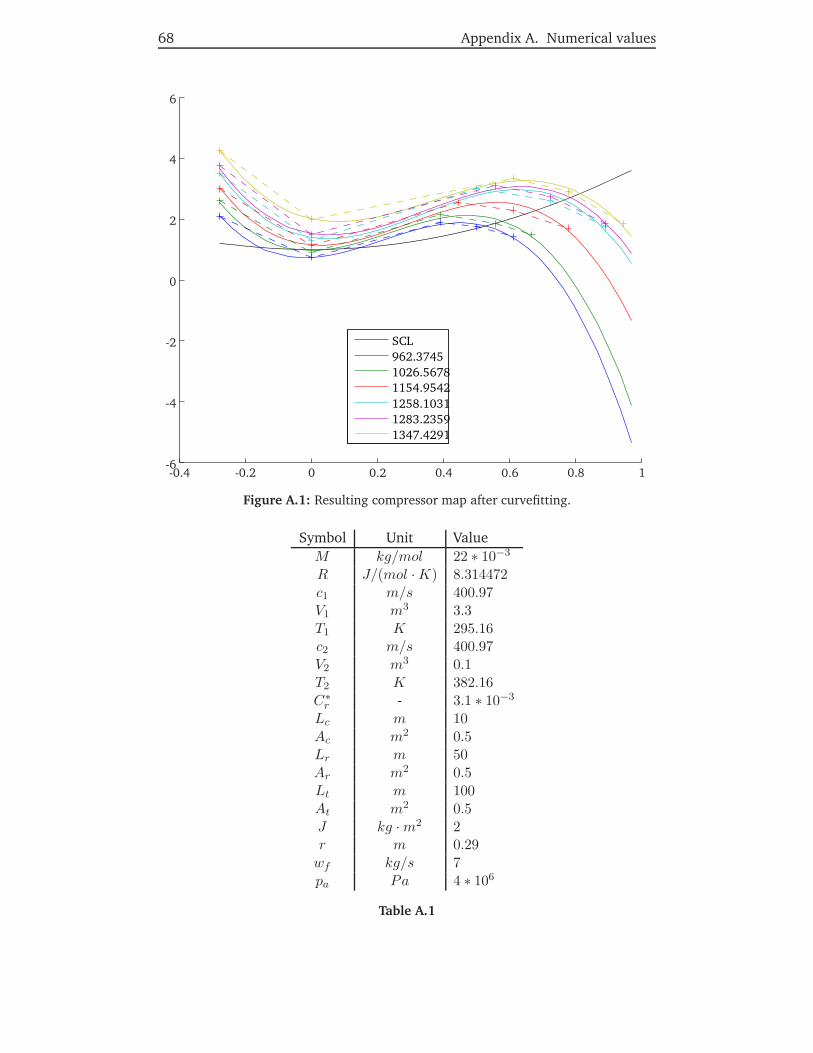
68 Appendix A. Numerical values
SCL962.37451026.56781154.95421258.10311283.23591347.4291
-0.4 -0.2 0 0.2 0.4 0.6 0.8 1-6
-4
-2
0
2
4
6
Figure A.1: Resulting compressor map after curvefitting.
Symbol Unit ValueM kg/mol 22 ∗ 10−3
R J/(mol ·K) 8.314472c1 m/s 400.97V1 m3 3.3T1 K 295.16c2 m/s 400.97V2 m3 0.1T2 K 382.16C∗r - 3.1 ∗ 10−3
Lc m 10Ac m2 0.5Lr m 50Ar m2 0.5Lt m 100At m2 0.5J kg ·m2 2r m 0.29wf kg/s 7pa Pa 4 ∗ 106
Table A.1
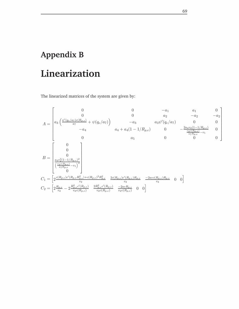
69
Appendix B
Linearization
The linearized matrices of the system are given by:
A =
⎡⎢⎢⎢⎢⎢⎢⎢⎣
0 0 −a1 a1 00 0 a2 −a2 −a2
a3
(ψ′(qe/a7)c(Rp,e)
a7+ ψ(qe/a7)
)−a3 a3ψ
′(qe/a7) 0 0
−a4 a4 + a4(1 − 1/Rp,e) 0 −2a4v2(1−1/Rp,e)v2c(Rp,e)
a7Rp,e−v1
0
0 a5 0 0 0
⎤⎥⎥⎥⎥⎥⎥⎥⎦
B =
⎡⎢⎢⎢⎢⎢⎢⎣
000
a4v32(1−1/Rp,e)2(v2c(Rp,e)
a7Rp,e−v1
)2
0
⎤⎥⎥⎥⎥⎥⎥⎦
C1 =[2 c(Rp,e)c′(Rp,eR2
p,e)+c(Rp,e)2R2p,e
v2
2c(Rp,e)c′(Rp,e)Rp,e
v2
−2a7c(Rp,e)Rp,e
v20 0
]C2 =
[2Rp,e
v2− 2R
2p,ec
′(Rp,e)
v2c(Rp,e)
2R2p,ec
′(Rp,e)
v2c(Rp,e)−2a7Rp,e
v2c(Rp,e)0 0
]


71
Appendix C
Transfer functions
D (f) (xe) =∂f
∂x|x=xe
C.1 Strategy 1
Nu(s) = n3s3 + n2s
2 + n1s+ n0
n3 = −2 a4 v22 (Rp,e − 1)2 (a1 D (c) (Rp,e)Rp,e − a1 c (Rp,e)
+ D (c) (Rp,e) a2 ) a73c (Rp,e)Rp,e
2
n2 =−2 a4 v22 (Rp,e −1)2
(−a1 D (c) (Rp,e)Rp,e a3 D (ψc)
(c (Rp,e)
a7
)+a3 a2 a7
− D (c) (Rp,e) a2 D (ψc)(c (Rp,e)
a7
)a3 + a7 a3 a1 Rp,e
)a7
3c (Rp,e)Rp,e2
n1 = −2 a4 v22 (Rp,e − 1)2 (a1 D (c) (Rp,e)Rp,e a5 a2
− a1 c (Rp,e) a5 a2 ) a73c (Rp,e)Rp,e
2
n0 = −2 (Rp,e − 1)2 v22a4
(a3 a5 a2 a1 Rp,e a7
− a1 D (c) (Rp,e)Rp,e a5 a2 D (ψc)(c (Rp,e)
a7
)a3
)a7
3c (Rp,e)Rp,e2
Du(s) = d5s5 + d4s
4 + d3s3 + d2s
2 + d1s+ d0
d5 = (−v2c (Rp,e) + v1a7 Rp,e)(−a7 Rp,e v2c (Rp,e) + Rp,e
2a72v1)

72 Appendix C. Transfer functions
d4 = (−v2c (Rp,e) + v1a7 Rp,e)(
Rp,e v2c (Rp,e) a3 D (ψc)(c (Rp,e)
a7
)a7
− v1a72Rp,e
2a3 D (ψc)(c (Rp,e)
a7
)− 2 a4 a7
2v2Rp,e2 + 2 a4 a7
2v2Rp,e
)
d3 = (−v2c (Rp,e) + v1a7 Rp,e)(
2 a4 a2 v1a72Rp,e
2 + a1 a72a3 Rp,e
3v1
+ Rp,e v2 (c (Rp,e))2 a3 a1 D (ψc)
(c (Rp,e)
a7
)+ a4 a1 v1a7
2Rp,e2
− a7 a5 a2 Rp,e v2c (Rp,e) + a4 a2 v2c (Rp,e) a7 + a72a5 a2 v1Rp,e
2
− Rp,e a4 a1 v2c (Rp,e) a7 − 2 a4 a72v2Rp,e a3 D (ψc)
(c (Rp,e)
a7
)
− a1 a7 a3 Rp,e2v2c (Rp,e) + 2 a4 a7
2v2Rp,e2a3 D (ψc)
(c (Rp,e)
a7
)
+ v1a72Rp,e
2a3 a2 − v1a7 Rp,e2a3 a1 D (ψc)
(c (Rp,e)
a7
)c (Rp,e)
− Rp,e v2c (Rp,e) a3 a2 a7 − a4 a2 v1a72Rp,e − 2 a4 a2 v2Rp,e c (Rp,e) a7
)
d2 = (−v2c (Rp,e) + v1a7 Rp,e)(
2 a4 a7 v2Rp,e2a3 a1 D (ψc)
(c (Rp,e)
a7
)c (Rp,e)
+ 2 a72a5 a2 a4 v2Rp,e − a4 a1 v1a7
2Rp,e2a3 D (ψc)
(c (Rp,e)
a7
)
− 2 a1 a72Rp,e
3a4 v2a3 − a4 a7 v2Rp,e a3 a1 D (ψc)(c (Rp,e)
a7
)c (Rp,e)
+ 2 a1 a72Rp,e
2a4 v2a3 − 2 a72a5 a2 a4 v2Rp,e
2
+ 2 a4 a2 v2Rp,e c (Rp,e) a3 D (ψc)(c (Rp,e)
a7
)a7
− 2 a4 a2 v1a72Rp,e
2a3 D (ψc)(c (Rp,e)
a7
)
+ a4 a2 v1a72Rp,e a3 D (ψc)
(c (Rp,e)
a7
)+ 2 a4 a7
2v2Rp,e a3 a2
− a72a3 a5 a2 D (ψc)
(c (Rp,e)
a7
)v1Rp,e
2 − 2 a4 a72v2Rp,e
2a3 a2
− a4 a2 v2c (Rp,e) a3 D (ψc)(c (Rp,e)
a7
)a7
+ a7 a3 a5 a2 D (ψc)(c (Rp,e)
a7
)Rp,e v2c (Rp,e)
)

Appendix C. Transfer functions 73
d1 = (−v2c (Rp,e) + v1a7 Rp,e)(
a1 a72a3 Rp,e
3a5 a2 v1
+ 2 a72a3 a5 a2 D (ψc)
(c (Rp,e)
a7
)a4 v2Rp,e
2
− a1 a7 a3 a5 a2 D (ψc)(c (Rp,e)
a7
)c (Rp,e) v1Rp,e
2
− a1 a7 a5 a2 Rp,e a4 v2c (Rp,e) + a1 a72a5 a2 a4 v1Rp,e
2
+ a1 a3 a5 a2 D (ψc)(c (Rp,e)
a7
)(c (Rp,e))
2 Rp,e v2
− a1 a7 a3 Rp,e2a5 a2 v2c (Rp,e)
− 2 a72a3 a5 a2 D (ψc)
(c (Rp,e)
a7
)a4 v2Rp,e
)
d0 = (−v2c (Rp,e)
+ v1a7 Rp,e)(−a1 a7 a3 a5 a2 D (ψc)
(c (Rp,e)
a7
)c (Rp,e) a4 v2Rp,e
− 2 a1 a72a3 Rp,e
3a5 a2 a4 v2 + 2 a1 a72a3 Rp,e
2a5 a2 a4 v2
+ 2 a1 a7 a3 a5 a2 D (ψc)(c (Rp,e)
a7
)c (Rp,e) a4 v2Rp,e
2
− a1 a72a3 a5 a2 a4 v1Rp,e
2D (ψc)(c (Rp,e)
a7
))
C.2 Strategy 2
Nu(s) = n3s3 + n2s
2 + n1s+ n0
n3 = −2 a4 v22 (Rp,e − 1)2 (a1 D (c) (Rp,e)Rp,e − a1 c (Rp,e)
+ D (c) (Rp,e) a2 ) a73Rp,e
2
n2 =−2 a4 v22 (Rp,e −1)2
(−a1 D (c) (Rp,e)Rp,e a3 D (ψc)
(c (Rp,e)
a7
)+a3 a2 a7
− D (c) (Rp,e) a2 D (ψc)(c (Rp,e)
a7
)a3 + a7 a3 a1 Rp,e
)a7
3Rp,e2
n1 = −2 a4 v22 (Rp,e −1)2 (a1 D (c) (Rp,e)Rp,e a5 a2 −a1 c (Rp,e) a5 a2 ) a7
3Rp,e2
n0 = −2 a4 v22 (Rp,e − 1)2
(a3 a5 a2 a1 Rp,e a7
− a1 D (c) (Rp,e)Rp,e a5 a2 D (ψc)(c (Rp,e)
a7
)a3
)a7
3Rp,e2

74 Appendix C. Transfer functions
Du(s) = d5s5 + d4s
4 + d3s3 + d2s
2 + d1s+ d0
d5 = c (Rp,e) (−v2c (Rp,e) + v1a7 Rp,e)(−a7 Rp,e v2c (Rp,e) + Rp,e
2a72v1)
d4 = c (Rp,e) (−v2c (Rp,e) + v1a7 Rp,e)(
Rp,e v2c (Rp,e) a3 D (ψc)(c (Rp,e)
a7
)a7
− v1a72Rp,e
2a3 D (ψc)(c (Rp,e)
a7
)− 2 a4 a7
2v2Rp,e2 + 2 a4 a7
2v2Rp,e
)
d3 = c (Rp,e) (−v2c (Rp,e) + v1a7 Rp,e)(
2 a4 a2 v1a72Rp,e
2 + a1 a72a3 Rp,e
3v1
+ Rp,e v2 (c (Rp,e))2 a3 a1 D (ψc)(c (Rp,e)
a7
)+ a4 a1 v1a7
2Rp,e2
− a7 a5 a2 Rp,e v2c (Rp,e) + a4 a2 v2c (Rp,e) a7 + a72a5 a2 v1Rp,e
2
− Rp,e a4 a1 v2c (Rp,e) a7 − 2 a4 a72v2Rp,e a3 D (ψc)
(c (Rp,e)
a7
)
− a1 a7 a3 Rp,e2v2c (Rp,e) + 2 a4 a7
2v2Rp,e2a3 D (ψc)
(c (Rp,e)
a7
)
+ v1a72Rp,e
2a3 a2 − v1a7 Rp,e2a3 a1 D (ψc)
(c (Rp,e)
a7
)c (Rp,e)
− Rp,e v2c (Rp,e) a3 a2 a7 − a4 a2 v1a72Rp,e − 2 a4 a2 v2Rp,e c (Rp,e) a7
)
d2 = c (Rp,e) (−v2c (Rp,e)
+ v1a7 Rp,e)(
2 a4 a7 v2Rp,e2a3 a1 D (ψc)
(c (Rp,e)
a7
)c (Rp,e)
+ 2 a72a5 a2 a4 v2Rp,e − a4 a1 v1a7
2Rp,e2a3 D (ψc)
(c (Rp,e)
a7
)
− 2 a1 a72Rp,e
3a4 v2a3 − a4 a7 v2Rp,e a3 a1 D (ψc)(c (Rp,e)
a7
)c (Rp,e)
+ 2 a1 a72Rp,e
2a4 v2a3 − 2 a72a5 a2 a4 v2Rp,e
2
+ 2 a4 a2 v2Rp,e c (Rp,e) a3 D (ψc)(c (Rp,e)
a7
)a7
− 2 a4 a2 v1a72Rp,e
2a3 D (ψc)(c (Rp,e)
a7
)
+ a4 a2 v1a72Rp,e a3 D (ψc)
(c (Rp,e)
a7
)+ 2 a4 a7
2v2Rp,e a3 a2
− a72a3 a5 a2 D (ψc)
(c (Rp,e)
a7
)v1Rp,e
2 − 2 a4 a72v2Rp,e
2a3 a2
− a4 a2 v2c (Rp,e) a3 D (ψc)(c (Rp,e)
a7
)a7
+ a7 a3 a5 a2 D (ψc)(c (Rp,e)
a7
)Rp,e v2c (Rp,e)
)

Appendix C. Transfer functions 75
d1 = c (Rp,e) (−v2c (Rp,e) + v1a7 Rp,e)(
a1 a72a3 Rp,e
3a5 a2 v1
+ 2 a72a3 a5 a2 D (ψc)
(c (Rp,e)
a7
)a4 v2Rp,e
2
− a1 a7 a3 a5 a2 D (ψc)(c (Rp,e)
a7
)c (Rp,e) v1Rp,e
2
− a1 a7 a5 a2 Rp,e a4 v2c (Rp,e) + a1 a72a5 a2 a4 v1Rp,e
2
+ a1 a3 a5 a2 D (ψc)(c (Rp,e)
a7
)(c (Rp,e))
2 Rp,e v2
− a1 a7 a3 Rp,e2a5 a2 v2c (Rp,e)
− 2 a72a3 a5 a2 D (ψc)
(c (Rp,e)
a7
)a4 v2Rp,e
)
d0 = c (Rp,e) (−v2c (Rp,e) + v1a7 Rp,e)(
a1 a72a3 Rp,e
3a5 a2 v1
+ 2 a72a3 a5 a2 D (ψc)
(c (Rp,e)
a7
)a4 v2Rp,e
2
− a1 a7 a3 a5 a2 D (ψc)(c (Rp,e)
a7
)c (Rp,e) v1Rp,e
2
− a1 a7 a5 a2 Rp,e a4 v2c (Rp,e) + a1 a72a5 a2 a4 v1Rp,e
2
+ a1 a3 a5 a2 D (ψc)(c (Rp,e)
a7
)(c (Rp,e))
2 Rp,e v2
− a1 a7 a3 Rp,e2a5 a2 v2c (Rp,e)
− 2 a72a3 a5 a2 D (ψc)
(c (Rp,e)
a7
)a4 v2Rp,e
)c (Rp,e) (−v2c (Rp,e)
+ v1a7 Rp,e)(−a1 a7 a3 a5 a2 D (ψc)
(c (Rp,e)
a7
)c (Rp,e) a4 v2Rp,e
− 2 a1 a72a3 Rp,e
3a5 a2 a4 v2 + 2 a1 a72a3 Rp,e
2a5 a2 a4 v2
+ 2 a1 a7 a3 a5 a2 D (ψc)(c (Rp,e)
a7
)c (Rp,e) a4 v2Rp,e
2
− a1 a72a3 a5 a2 a4 v1Rp,e
2D (ψc)(c (Rp,e)
a7
))


77
Appendix D
CD content
The attached CD contains the Simulink model used to run the presented simula-tions, along with scripts developed to describe the compressor map and strate-gies. To run, start MATLAB/Simulink and execute the file initConstants3 beforestarting the simulation.
The files included are:
Name FunctioninitConstants3.m Initializes all constants and finds equilibriainitCompressor3.m Creates compressormap from given data pointsrecycle_controller.m Computes the control variablecompressorMap3.m Computes the pressure ratio for given
inlet pressure and mass floweq_fun.m Finds the crossing between the SCL and
the desired speed lineSCL.m Give desired flow from desired pressure ratioSCLinv.m Give desired pressure ratio from desired flowcompressorV13openloop.mdl The Simulink model for the compression system