Closed-form solutions to static-arbitrage upper bounds on basket

options

Javier Pena∗1, Juan C. Vera†2, and Luis F. Zuluaga‡3

1Tepper School of Business, Carnegie Mellon University2Department of Management Sciences, University of Waterloo

3Faculty of Business Administration, University of New Brunswick

July 25, 2008

Abstract

We provide a closed-form solution to the problem of computing the sharpest static-arbitrageupper bound on the price of a European basket option, given the prices of vanilla call optionsin the underlying securities. Unlike previous approaches to this problem, our solution techniqueis entirely based on linear programming. This also allows us to obtain an efficient (linear-size) linear programming formulation for the more realistic problem of computing sharp staticarbitrage upper bounds taking into consideration bid-ask spreads in the given option prices andother transaction costs.

1 Introduction

We provide a closed-form solution to the problem of computing the sharpest upper bound onthe price of a European basket option, given the only assumption of absence of arbitrage, andinformation on the prices of vanilla European call options on the same underlying assets and withthe same maturity. Bounds of this type are called static-arbitrage bounds. These kinds of boundscan be seen as robust bounds that any sound pricing model must satisfy [5, 9]. They providea mechanism for checking consistency of prices, as well as an initial price estimate for optionsregardless of any model specifics.

The computation of sharp static-arbitrage upper bounds can be formulated as the problem offinding an underlying asset price distribution that maximizes the discounted expected payoff ofthe basket option, and replicates the given option prices [3]. Under reasonably mild assumptions(see, e.g., Proposition 1 in Section 2), an equivalent dual formulation is to find the least expensiveportfolio of cash and the options with known prices whose combined payoff super-replicates thepayoff of the new basket option of interest (see, e.g. [3, 9]). This semiparametric approach can beseen as an alternative to parametric techniques (such as Monte Carlo simulations) that determinethe price of an option as the discounted expected option’s payoff under an appropriate risk-neutralmeasure. Semiparametric techniques are especially useful in incomplete market conditions, or∗jfp@andrew.cmu.edu†jvera@uwaterloo.ca‡lzuluaga@unb.ca

1

when the number of underlying assets makes the computation of parametric prices numericallychallenging.

The problem of computing static-arbitrage bounds has received a fair amount of attention inrecent years. Of particular relevance to our work are the recent articles by d’Aspremont and ElGhaoui [3], and by Hobson, Laurence, and Wang [8, 9]. D’Aspremont and El Ghaoui [3] derivelinear programming relaxations for static-arbitrage bounds based on an integral transformation ofthe options’ price functions. They show that their bounds are tight in some special cases whenonly one or two vanilla options prices per underlying asset are given. On the other hand, Hobson,Laurence and Wang [8, 9] derive more general results for computing sharp static-arbitrage upperbounds when vanilla option prices on every asset are given for a continuum of strikes. Theirapproach relies on a Lagrangian programming formulation and the fact that the continuum ofoptions determines the full marginal distributions of each of the assets.

We undertake a fairly different and novel approach to the static arbitrage upper bound problembased entirely on linear programming techniques. The foundational block of our work is the con-struction of an efficient (linear-size) polyhedral description for the set of super-replicating portfolios,that is, the set of portfolios of cash and the given options whose payoff super-replicates the basketoption’s payoff. We show that the set of super-replicating portfolios is a projection of a polyhedronwhose description only requires a number of variables and constraints that is linear in the numberof given options (see Lemma 6). The polyhedral description yields an efficient linear programmingformulation for the static-arbitrage upper bound problem that can be solved in closed form (seeTheorem 3). The latter generalizes a result of d’Aspremont and El Ghaoui [3] that was previouslyknown only for basket options with positive weights in the special case when one or two vanillaoption prices per underlying asset are given. Furthermore, the polyhedral description readily al-lows us to obtain efficient models that incorporate for the first time some important features inthe static bounds’ computations. Some of these features are basket options with negative weights,bid-ask spreads, limits on the sizes of long/short positions, and transaction costs. Moreover, theclosed-form formula provided by Theorem 3 has an interesting application in the derivation of arobust portfolio allocation model [6].

Although it is intuitively clear that the set of super-replicating portfolios admits a polyhedraldescription, straightforward attempts to do so yield intractable descriptions that require a numberof constraints and variables that is exponentially large in the number of given option prices. Bycontrast, we provide a polyhedral description whose number of variables and constraints is onlylinear in the number of given option prices. We note that the computation of static arbitrage lowerbounds poses a different set of challenges as the nature of sub-replicating portfolios is fundamentallydifferent from that of the super-replicating portfolios. The different nature of the upper and lowerbound computation has been recognized previously, as it was apparent that the computation ofthe upper bounds was more tractable [3, 8, 9]. A separate article [11] presents some results for thecomputation of static arbitrage lower bounds that are similar in spirit to those discussed herein.

We note in passing that an interesting and active related area of research is the computation ofoption price bounds given moment information about the underlying risk-neutral asset price dis-tribution. These kinds of bounds have been investigated in the work of Bertsimas and Popescu [1],Boyle and Lin [2], and Zuluaga and Pena [14] among others. This moment approach to computeoption price bounds differs from the computation of arbitrage bounds studied here in two mainaspects: First, in the moment approach an underlying model for the risk neutral asset prices dis-tribution is assumed in order to sample (obtain) the necessary moment information. By contrast,the arbitrage approach relies solely on option price information observed in the market. Second,the computation of moment-based bounds in general requires the use of semidefinite programmingsolvers whereas arbitrage bounds can be computed via linear programming.

2

The paper is organized as follows. Section 2 presents the basic notation and closed-form solutionto the static arbitrage upper bound on a basket option, given the prices of vanilla call options onthe underlying assets. In Section 3 we present the main building block of our approach, namely anefficient polyhedral description of the super-replicating portfolios. The latter yields the first efficientlinear programming formulation for the computation of static arbitrage bounds that incorporatebid-ask spreads. In Section 4 we provide numerical experiments to illustrate some of our results.Finally, Section 5 presents the proofs of the results in the paper.

2 Static-arbitrage bounds

Consider the problem of computing a sharp upper static-arbitrage bound on the price of a Euro-pean basket option, given information on the prices of other similar options, without making anyassumptions other than the absence of arbitrage. This problem can be formulated as the followingoptimization problem (see, e.g., [3]):

supπ

Eπ[(ω · S − κ)+]

s.t. Eπ[1] = 1Eπ[(wj · S −Kj)+] = pj , j = 1, ..., rπ a distribution in Rn

+.

(U)

Above, the multivariate random variable S with probability distribution π represents the prices ofthe n underlying assets (at maturity) in the basket. The vectors wj ∈ Rn, and constants Kj ∈ R,j = 1, . . . , r, represent the weights of the underlying assets and the strike price of the basket optionswhose prices are given. The vector ω ∈ Rn and constant κ ∈ R represent the weights and strike ofthe basket option whose price we want to bound. Problem (U) maximizes the expected payoff ofthe basket option (ω · S − κ)+ over all underlying asset price distributions π in Rn

+ that replicatethe price pj of the basket option (wj · S −Kj)+ for j = 1, . . . , r.

Following [3], we implicitly assume that all the options have the same maturity, and that withoutloss of generality, the risk-free interest rate is zero; or equivalently, we compare the prices in theforward market (at maturity).

Problem (U) has the following associated dual (see, [7]):

infz,y

z +r∑j=1

pjyj

s.t. z +r∑j=1

yj(wj · s−Kj)+ ≥ (ω · s− κ)+ for all s ∈ Rn+

y ∈ Rr, z ∈ R.

(DU)

The dual problem has a natural financial interpretation: Find the cheapest portfolio of positionsin cash and in the basket options (wj · S − Kj)+, j = 1, . . . , r that super-replicates the payoffof the basket option (ω · S − κ)+. It is easy to see that weak duality holds between (U) and(DU). Furthermore, under reasonably mild assumptions, strong duality holds as well. For instance,Proposition 1 states two generic conditions that ensure strong duality in our context.

Proposition 1. The optimal values of (U) and (DU) coincide —i.e., strong duality holds between(U) and (DU)— if at least one of the following two conditions holds.

3

(i) Strong primal feasibility:[1p

]∈ int

({[Eπ[1](

Eπ[(wj · S −Kj)+)j=1,...,r

]

]: π is a distribution in Rn

+

}).

In particular, strong duality holds provided the prices p are arbitrage-free and remain arbitrage-free after slight perturbations.

(ii) Strong dual feasibility: There exists (z, y) ∈ Rr+1 such that

(z, y) ∈ int

(z, y) ∈ Rr+1 : z +r∑j=1

yj(wj · s−Kj)+ ≥ (ω · s− κ)+ for all s ∈ Rn+

.

In particular, strong duality holds provided that for each asset at least one vanilla option priceis known.

Proposition 1 follows from general convex duality results [12, 13]. A detailed discussion can befound in [14, Sec. 3].

The lower static-arbitrage bound on the price of a basket option corresponding to (U) can beobtained by changing sup to inf in (U). For some recent advances on this problem, see [8, 11].

2.1 Upper bound given calls on single assets

We next consider the computation of the upper bound on the price of the basket (ω ·S−κ)+ in thespecial but important case when prices of m calls pji = Eπ[(Si−Kj

i )+], j = 1, . . . ,m and a forward

p0i = Eπ[Si] for each asset i = 1, . . . , n are known. Notice that the assumption on the same number

of options m per asset can be made without loss of generality: If one of the assets has fewer thanm options, we can artificially increase the number of known options to m by repeating one of theoptions.

In this case the static upper bound problem (U) is

supπ

Eπ[(ω · S − κ)+]

s.t. Eπ[1] = 1Eπ[S] = p0

Eπ[(S −Kj)+] = pj , j = 1, . . . ,mπ a distribution in Rn

+.

(1)

Here and throughout the sequel we use the following convenient vector notation: Eπ[(S−Kj)+] = pj

is a shorthand for Eπ[(Si −Kji )

+] = pji , for i = 1, . . . , n.

Without loss of generality assume:

~0 ≤ K1 ≤ · · · ≤ Km ∈ Rn.

It is convenient to put K0 := ~0 so that the dual (DU) of (1) can be written as

infz,y0,...,ym

z +m∑j=0

pj · yj

s.t. z +m∑j=0

yj · (s−Kj)+ ≥ (ω · s− κ)+ for all s ∈ Rn+

yj ∈ Rn, j = 0, . . . ,mz ∈ R.

(2)

4

By Proposition 1(ii), the optimal values of (1) and (2) are the same. We shall assume that foreach asset the given forward and call prices are arbitrage-free. This can be done without loss ofgenerality as otherwise the static-arbitrage problem (1) is infeasible and hence uninteresting.

Theorem 3 below provides a closed-form expression for this bound under the arbitrage-freeassumption. In addition, Theorem 5 provides a closed-form expression for the optimal super-replicating strategy that solves (2). We note that the closed-form formula (5) generalizes theclosed-form formula derived by d’Aspremont and El Ghaoui [3, Prop.4]. The latter corresponds to(5) for the special case m = 1 and ω ≥ 0.

It is well-known [1] that a set of vanilla options (Si − Kji )

+, j = 0, 1, . . . ,m in asset i isarbitrage-free if and only if the following convexity condition holds:

0 ≤pm−1i − pmi

Kmi −K

m−1i

≤pm−2i − pm−1

i

Km−1i −Km−2

i

≤ · · · ≤ p1i − p2

i

K2i −K1

i

≤ p0i − p1

i

K1i

≤ 1. (3)

Thus, the arbitrage-free assumption can be stated as follows.

Assumption 2. Condition (3) holds for each i = 1, . . . , n.

We note that Davis and Hobson [4] provide an interesting generalization of the arbitrage-freecondition (3) to the multiperiod setting.

Before stating the closed-form expression for the bound (1), we introduce some convenientnotation. Define

I+ := {i ∈ {1, . . . , n} : ωi ≥ 0} , I− := {i ∈ {1, . . . , n} : ωi < 0} ,

and let ν : [0, 1]→ Rn be defined as

ν(τ)i =

min

j=0,...,m

{pji + τKj

i

}if i ∈ I+

p0i − min

j=0,...,m

{pji + (1− τ)Kj

i

}if i ∈ I−.

(4)

Theorem 3. Suppose Assumption 2 holds. Then the optimal value of (1) is

maxτ∈[0,1]

(ω · ν(τ)− τκ). (5)

Remark 4. Because the components of ν(τ) are piecewise linear, the value (5) can be found byevaluating the breakpoints where the components of ν(τ) change slopes, that is, the mn+ 2 points:

τ = 0, 1, τ =pj−1i − pji

Kji −K

j−1i

, i ∈ I+, and τ = 1−pj−1i − pji

Kji −K

j−1i

, i ∈ I−, j = 1, . . . ,m. (6)

Furthermore, because each ωi · ν(τ)i is concave, it follows that the function ω · ν(τ)− τκ is concaveas well. Thus once the mn + 2 breakpoints in (6) are sorted, the one-dimensional optimizationproblem (5) can be solved via a binary search by evaluating ω · ν(τ)− τκ at 2 log(nm+ 2) points.

We next describe the optimal super-replicating strategy that solves (2) and yields the optimalbound (5). To that end, we introduce some additional convenient notation. Assume τ ∈ [0, 1] isgiven. For each i = 1, . . . , n let ji[τ ], j′i[τ ] denote the indices where the relevant minimum in (4) isattained. More precisely, for each i ∈ I+ let ji[τ ] and j′i[τ ] be such that

ν(t)i = pji[τ ]i + tK

ji[τ ]i for t ↓ τ, and ν(t)i = p

j′i[τ ]i + tK

j′i[τ ]i for t ↑ τ.

5

Likewise, for each i ∈ I− let ji[τ ] and j′i[τ ] be such that

ν(t)i = p0i − (pji[τ ]i + (1− t)Kji[τ ]

i ) for t ↓ τ, and ν(t)i = p0i − (pj

′i[τ ]i + (1− t)Kj′i[τ ]

i ) for t ↑ τ.

Notice that j′i[τ ] = ji[τ ]± 1 if τ is one of the relevant breakpoints (6) for ν(τ)i, and otherwisej′i[τ ] = ji[τ ].

Theorem 5. Suppose Assumption 2 holds. Let τ be the maximizer of (5).

(a) If τ ∈ (0, 1) thenn∑i=1

ωiKji[τ ]i ≤ κ ≤

n∑i=1

ωiKj′i[τ ]i . Consequently, there exists λ ∈ [0, 1] such that

n∑i=1

ωi

(λK

ji[τ ]i + (1− λ)Kj′i[τ ]

i

)= κ, (7)

and an optimal solution to (2) is

z =∑i∈I−

ωi

(−λKji[τ ]

i − (1− λ)Kj′i[τ ]i

)yji[τ ]i = λ|ωi|, y

j′i[τ ]i = (1− λ)|ωi|, for i = 1, . . . , n

y0i = ωi for i ∈ I−yji = 0 for all other i, j.

(8)

In the case ji[τ ] = j′i[τ ] = j, the second equation in (8) is to be interpreted as yji = yji[τ ]i +

yj′i[τ ]i = |ωi|.

(b) If τ = 0 then an optimal solution to (2) is

z = −∑i∈I−

ωiKji[τ ]i

yji[τ ]i = |ωi| for i = 1, . . . , ny0i = ωi for i ∈ I−yji = 0 for all other i, j.

(c) If τ = 1 then an optimal solution to (2) is

z = −∑i∈I+

ωiKj′i[τ ]i − κ

yj′i[τ ]i = |ωi| for i = 1, . . . , ny0i = ωi for i ∈ I−yji = 0 for all other i, j.

3 Super-replicating portfolios

In this section we describe the main foundational block of our approach, namely an efficient polyhe-dral description for the set of super-replicating portfolios, i.e., the set of portfolios (y0, y1, . . . , ym, z)that satisfy the constraints in (2).

6

3.1 Super-replication of a linear payoff

Assume K =[K0 K1 · · · Km

]∈ Rn×(m+1), b ∈ Rn and c ∈ R are given. Define the set of

super-replicating strategies SR(K, b, c) as follows

SR(K, b, c) := {(y, z) = (y0, y1, . . . , ym, z) ∈ Rn×(m+1)×R : z+m∑j=0

yj ·(s−Kj)+ ≥ b·s−c for all s ∈ Rn+}.

The set SR(K, b, c) is the set of combinations of the call options (s −Kji )

+ and cash that super-replicate the linear payoff b · s− c.

As Lemma 6 below states, the set SR(K, b, c) is a projection of the lifted polyhedron LSR(K, b, c).The latter is a set in a higher dimensional space with an efficient polyhedral description. DefineLSR(K, b, c) as the set of points (y, z, γ, β, ξ) ∈ Rn×(m+1) × R × Rn×(m+1)

+ × Rn×m+ × Rn that

satisfyi∑

j=0

yj − b = γi − βi, i = 0, . . . ,m− 1

m∑j=0

yj − b = γm

i∑j=0

Kj ◦ yj ≤ ξ +Ki ◦ γi −Ki+1 ◦ βi, i = 0, . . . ,m− 1

m∑j=0

Kj ◦ yj ≤ ξ +Km ◦ γm

−z − c ≤ −e · ξ.

(9)

Here u ◦ v ∈ Rn denotes the Hadamark product of u, v ∈ Rn, i.e., (u ◦ v)i = uivi, i = 1, . . . , n,and e ∈ Rn is the vector of all ones. Note that the number of variables and constraints in thedescription of LSR(K, b, c) is proportional to mn, i.e., to the number of known option prices.

Lemma 6. Assume ~0 = K0 ≤ K1 ≤ · · · ≤ Km ∈ Rm and b ∈ Rn, c ∈ R are given. Then(y, z) ∈ SR(K, b, c) if and only if there exist γ ∈ Rn×(m+1)

+ , β ∈ Rn×m+ , and ξ ∈ Rn such that

(y, z, γ, β, ξ) ∈ LSR(K, b, c).

3.2 Static arbitrage upper bounds with bid-ask spreads

As we detail in Section 5, both Theorem 3 and Theorem 5 follow from Lemma 6. Furthermore,Lemma 6 readily yields efficient (linear-size) linear programming formulations for variations ofthe problem (2) that incorporate important additional features that have not been treated before.In particular, we next present an efficient linear programming formulation for the static arbitragebound problem that takes into account bid-ask spreads in the prices of the known options. Previousapproaches to the computation of arbitrage bounds [3, 8, 9] ignore this important feature and simplyassume that the known options can be bought and sold at a mid-market price. This constitutes amajor practical limitation as these mid-market prices are rarely arbitrage-free. One of our numericalexamples in Section 4 illustrates this phenomenon.

Assume the vector of ask (buying) and bid (selling) prices of the options (S−Kj)+ are pj+ ≥ pj−

7

respectively. In this case the optimal super-replication problem becomes

infz,y,y+,y−

z +m∑j=0

(pj+ · yj+ − p

j− · y

j−)

s.t. z +m∑j=0

yj · (s−Kj)+ ≥ (ω · s− κ)+ for all s ∈ Rn+

y = y+ − y−y ∈ Rn×(m+1)

y+, y− ∈ Rn×(m+1)+

z ∈ R.

(10)

This gives the lowest upper bound on the bid price of the option (ω · S − κ)+ that is implied bythe options (Si −Kj

i )+, i = 1, . . . , n, j = 0, . . . ,m, taking into consideration the bid-ask spreads.

Although problem (10) does not have a closed-form expression, Lemma 6 enables us to recastit as a linear program whose number of variables and constraints is proportional to mn, i.e., to thenumber of known option prices.

Theorem 7. The optimal super-replication problem (10) can be rewritten as

minz,y,y+,y−,γ,β,ξ,γ,β,ξ

z +m∑j=0

(pj+ · y

j+ − p

j− · y

j−

)s.t. (y, z, γ, β, ξ) ∈ LSR(K,ω, κ)

(y, z, γ, β, ξ) ∈ LSR(K, 0, 0)y = y+ − y−y+, y− ∈ Rn×(m+1)

+ .

(11)

Remark 8. The polyhedral description given by Lemma 6 allows the efficient modeling of otherfeatures in the optimal super-replication problem such as other types of transaction costs as well asrestrictions on the positions of the super-replication strategy. Some of these features are illustratedin our numerical experiments in Section 4.

4 Some numerical results

We next present computational experiments that illustrate some of our results. The experimentsfocus on the new features that can be incorporated as a result of our linear programming approach.In particular, we present a numerical example that takes into account the presence of bid-askspreads in option prices. We also discuss the possibility of adding diversification constraints to thesuper-replication strategy problem. Although these features are prevalent in real pricing problems,they were beyond the scope of previous approaches to static-arbitrage bounds. Finally, we consideran example with an exchange option, to illustrate how our approach allow us to consider basketoptions with negative weights.

Related numerical results are presented in [3, 9], where the authors provide extensive numericalexperiments comparing static-arbitrage pricing techniques and parametric pricing techniques (suchas Monte Carlo simulations) for basket options.

4.1 Bid-ask prices

In the formulation of the upper static-arbitrage bound (2), it is assumed that the options can bebought and sold at the same price. In practice, the price at which an investor buys the option, i.e.,

8

the ask price, is higher that the price at which the investor can sell the option, i.e., the bid price.This gives rise to the so-called bid-ask spread as can be observed in Table 1, which lists the prices ofvanilla options on stocks in the DJX index as traded on May 17th, 2004 on the June contracts withmaturity on June 18th, 2004. This dataset is similar to that of [9, Section 6.2, Table 2]. However,we have only included traded contracts (with volume greater than zero), for liquidity considerations.With the data in Table 1, we can use the linear programming formulation (11) in Section 3.2 tocompute the cheapest super-replicating strategy for the DJX basket call option with strike price80.00 taking into account the bid-ask spread. We obtain the super-replication strategy given inTable 2, which yields an upper bound of 19.8872. From market data, the best bid price for thisoption was 18.7, and the best ask price was 19.5. Table 2 provides the long (buy) positions on thecall options with position different from zero in the super-replicating portfolio. In this particularexperiment, the super-replicating portfolio does not contain any short (sell) positions.

Using bid and ask prices in the computation of the super-replicating strategy gives a morepractical value to the static-arbitrage pricing approach. In particular, this resolves a major limi-tation in previous approaches [3, 9] that used mid-market prices (e.g., the average of the bid andask prices) as the “nominal” option prices. Such approximation systematically underestimates theactual buying prices and overestimates the actual selling prices. It is then not surprising thatthe market data used in [3, 9] requires a fair amount of “cleaning” to rule out apparent arbitrageopportunities created by these estimates (see [9, Section 6.2]). By contrast, the model herein thattakes into account bid-ask spreads does not suffer from this limitation.

We note that although the super-replicating strategy in Table 2 contains only long positions,this does not mean that the bid-ask DJX option price upper bound of 19.8872 could be found bysimply using the ask (buy) prices as the option prices in the linear programming formulation ofthe problem (2). If this naive approach were attempted, the linear program would be unbounded,since the ask prices alone do not satisfy the arbitrage-free condition (3).

4.2 Diversifying the super-replicating strategy

Consider an investor looking at the strategy in Table 2, who wishes to create a super-replicatingstrategy that contains more positions in possible options, that is, a more diversified strategy. Toobtain such a super-replicating strategy we add the following diversifying linear constraints to theLP formulation (11), which ensure that the portfolio will have a position in each tier of options:

e · yj ≥ 0.05, j = 0, . . . ,m. (12)

Above e represents the vector of all-ones. The solution to this diversified super-replicating strat-egy gives a portfolio whose cost is 19.9022, just 0.08% more expensive than the cheapest super-replicating strategy computed in Table 2. As Table 3 shows, such a strategy has the desiredinvestor’s diversification preference.

4.3 Basket options with negative weights

Consider the problem of finding static-arbitrage bounds for a European exchange option, giventhe prices of vanilla options on the two assets involved. This corresponds to (1) with n = 2,ω =

[1 −1

]T, and κ = 0. We will consider the case in which information about the forward pricesof the two assets, and the following m = 5 call options is given:

K1 =[

0.850.85

], K2 =

[0.900.90

], K3 =

[0.950.95

], K4 =

[1.001.00

], K5 =

[1.051.05

]. (13)

9

To set up the problem, we sample the values of pj , j = 0, . . . , 5 in (1) corresponding to the strikesin (13), by assuming that the underlying asset prices distribution follows a correlated multivariatelognormal distribution (see, e.g., eq. (15) in [2]). In particular we use a riskless interest rate r = 0,option maturity T = 1, current prices S1(0) = 0.95, S2(0) = 0.90, volatilities δ1 = 0.2, δ2 = 0.22.Thus, we obtain (using Black-Scholes formula) the following given option prices for the problem:

p0 =[

0.95000.9000

], p1 =

[0.13240.1042

], p2 =

[0.10130.0788

],

p3 =[

0.07570.0584

], p4 =

[0.05520.0425

], p5 =

[0.03940.0304

].

(14)

The arbitrage condition (3) follows from computing the prices using the lognormal model. Thus,using Theorem 3, we obtain an upper static-arbitrage bound on the exchange option of 0.1802.Clearly, from the choice of the option prices in (14), it follows that the upper bound of 0.1802 mustbe higher than any exact price of the option computed by assuming that the underlying asset pricesfollow a lognormal distribution that replicates the option prices in (14). Indeed, using Magrabe’sformula [10], the exact price of the exchange option would ranges between [0.1361, 0.1801] if thecorrelation of the Wiener processes driving the lognormal distribution are negatively correlated,and between [0.0500, 0.1361] if they are positively correlated.

5 Proofs

5.1 Proof of Lemma 6.

The high level idea of the proof is to divide Rn+ in regions where each of the functions (s−Kj)+ is

linear. Using Farkas’ Lemma the set of super-replicating strategies in each region is a polyhedron.Thus the set of super-replicating strategies SR(K, b, c) is just the intersection of all these polyhedra,again a polyhedron. Since the number of regions is exponential, the number of variables andconstraints needed in a naive description of SR(K, b, c) is exponential. The main point of theproof is that we can “collapse” first the variables and then the constrains to obtain an efficientdescription, using only a linear number of variables and constraints.

Throughout this section we rely on the following convenient notation: Given a vector v ∈ Rn

and a set of indices I ⊆ {1, . . . , n}, we let vI denote the subvector of v obtained by selecting thecomponents of v indexed by I.

Proof of Lemma 6. Define the set of partitions P(n,m) of {1, . . . , n} as follows:

P(n,m) :=

{(J0, J1, . . . , Jm

):m⋃i=0

J i = {1, . . . , n} , J i ∩ J j = ∅ for i 6= j

}.

Given J ∈ P(n,m), define

PJ :={s : Ki

Ji ≤ sJi ≤ Ki+1Ji for i = 0, 1, . . . ,m− 1, and sJm ≥ Km

Jm

}.

Since {PJ : J ∈ P(n,m)} is a partition of Rn+, it follows that (y, z) ∈ SR(K, b, c) if and only if

z +m∑j=0

yj · (s−Kj)+ ≥ b · s− c for all s ∈ PJ for all J ∈ P(n,m). (15)

10

From the construction of {PJ : J ∈ P(n,m)}, it follows that each (si −Kji )

+ is linear on each PJ .Indeed, for s ∈ PJ we have

m∑j=0

yj · (s−Kj)+ =m∑i=0

i∑j=0

yjJi · (sJi −Kj

Ji).

Therefore, (15) is equivalent to

m∑i=0

−bJi +i∑

j=0

yjJi

· sJi ≥m∑i=0

i∑j=0

yjJi ·Kj

Ji − z − c for all s ∈ PJ for all J ∈ P(n,m).

By Farkas Lemma, the latter holds if and only if for each J ∈ P(n,m) there exist γi,J , βi,J ∈RJi

+ , i = 0, . . . ,m− 1, γm,J ∈ RJm

+ such that

−bJi +i∑

j=0

yjJi = γi,J − βi,J , i = 0, . . . ,m− 1

−bJm +m∑j=0

yjJm = γm,J

m∑i=0

i∑j=0

yjJi ·Kj

Ji

− z − c ≤ m−1∑i=0

(KiJi · γi,J −Ki+1

Ji · βi,J)

+KmJm · γm,J , J ∈ P(n,m).

(16)We will first reduce the number of variables used in this description of SR(K, b, c):

Claim 9. Assume (y0, . . . , ym, z) ∈ Rn × · · · × Rn × R is given. Then there exist γi,J , βi,J ∈RJi

+ , i = 0, . . . ,m− 1, γm,J ∈ RJm

+ for each J ∈ P(n,m) such that (16) holds if and only if thereexist γi, βi ∈ Rn

+, i = 0, . . . ,m− 1 and γm ∈ Rn+ such that

−b+i∑

j=0

yj = γi − βi, i = 0, . . . ,m− 1

−b+m∑j=0

yj = γm

m∑i=0

i∑j=0

yjJi ·Kj

Ji

− z − c ≤ m−1∑i=0

(KiJi · γiJi −Ki+1

Ji · βiJi

)+Km

Jm · γmJm , J ∈ P(n,m).

(17)

Then, we will reduce the number of constrains used in (17):

Claim 10. Assume (y, z, γ, β) ∈ Rn×(m+1) ×R×Rn×(m+1)+ ×Rn×m

+ is given. Then (17) holds ifand only if there exists ξ ∈ Rn such that (9) holds.

Claim 9 and Claim 10 show that (y, z) ∈ SR(K, b, c) if and only if there exist γ ∈ Rn×(m+1)+ , β ∈

Rn×m+ , and ξ ∈ Rn such that (y, z, γ, β, ξ) ∈ LSR(K, b, c).

Now we present the proofs of Claim 9 and Claim 10.

11

Proof of Claim 9. It is straightforward to check (17) implies (16). Assume (16) holds. Defineγm ∈ Rn

+ and γi, βi ∈ Rn+, i = 0, . . . ,m− 1 as follows. Let J = (∅, . . . , ∅, {1, . . . , n}) and put

γm := γm,J .

Then the second equation in (17) holds. Consequently, for any J ∈ P(n,m) we have

γmJm = −bJm +m∑j=0

yjJm = γm,J . (18)

Next, fix i ∈ {0, . . . ,m− 1}. For each ` ∈ {1, . . . , n} define the partition J [i, `] by

J [i, `] := argmax{J∈P(n,r):l∈Ji}

(Ki`γi,J` −K

i+1` βi,J`

).

Let γi, βi ∈ Rn+ be defined by γi` = γ

i,J [i,`]` and βi` = β

i,J [i,`]` , ` ∈ {1, . . . , n}. From the first identity

in (16), applied to J = J [i, `], we get

−bJ [i,`]i +i∑

j=0

yjJ [i,l]i

= γi,J [i,l] − βi,J [i,l].

In particular,

−b` +i∑

j=0

yj` = γi,J [i,`]` − βi,J [i,`]

` = γi` − βi`.

This holds for i ∈ {0, . . . ,m− 1} and ` ∈ {1, . . . , n} thus the first equation in (17) follows. It onlyremains to prove the last inequality in (17). To that end, fix J ∈ P(n,m). For i = 0, . . . ,m− 1 and` ∈ J i, the construction of J [i, `] implies that

Ki`γi,J` −K

i+1` βi,J` ≤ K

i`γi,J [i,`]` −Ki+1

` βi,J [i,`]` = Ki

`γi` −Ki+1

` βi`.

ThusKiJi · γi,J −Ki+1

Ji · βi,J ≤ KiJi · γiJi −Ki+1

Ji · βiJi .

Hence from the last inequality in (16) and (18) we get

m∑i=0

i∑j=0

yjJi ·Kj

Ji

− z − c ≤ m−1∑i=0

(KiJi · γi,J −Ki+1

Ji · βi,J)

+KmJm · γm,J

≤m−1∑i=0

(KiJi · γiJi

−Ki+1Ji · βiJi

)+Km

Jm · γmJm ,

completing the proof of the claim.

Proof of Claim 10. Assume (9) holds. Let J ∈ P(n,m) be given. From the third inequality in (9)we have

i∑j=0

KjJi · yjJi ≤ eJi · ξJi +Ki

Ji · γiJi −Ki+1Ji · βiJi , i = 0, . . . ,m− 1.

12

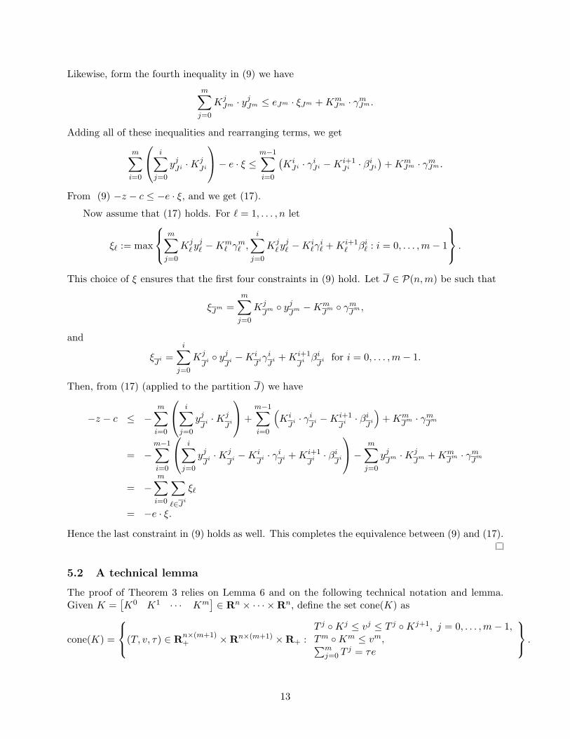
Likewise, form the fourth inequality in (9) we havem∑j=0

KjJm · yjJm ≤ eJm · ξJm +Km

Jm · γmJm .

Adding all of these inequalities and rearranging terms, we get

m∑i=0

i∑j=0

yjJi ·Kj

Ji

− e · ξ ≤ m−1∑i=0

(KiJi · γiJi −Ki+1

Ji · βiJi

)+Km

Jm · γmJm .

From (9) −z − c ≤ −e · ξ, and we get (17).

Now assume that (17) holds. For ` = 1, . . . , n let

ξ` := max

m∑j=0

Kj` yj` −K

m` γ

m` ,

i∑j=0

Kj` yj` −K

i`γi` +Ki+1

` βi` : i = 0, . . . ,m− 1

.

This choice of ξ ensures that the first four constraints in (9) hold. Let J ∈ P(n,m) be such that

ξJm =m∑j=0

Kj

Jm ◦ yj

Jm −Km

Jm ◦ γm

Jm ,

and

ξJ

i =i∑

j=0

Kj

Ji ◦ yj

Ji −Ki

Jiγi

Ji +Ki+1

Ji βi

Ji for i = 0, . . . ,m− 1.

Then, from (17) (applied to the partition J) we have

−z − c ≤ −m∑i=0

i∑j=0

yjJ

i ·Kj

Ji

+m−1∑i=0

(Ki

Ji · γi

Ji −Ki+1

Ji · βi

Ji

)+Km

Jm · γm

Jm

= −m−1∑i=0

i∑j=0

yjJ

i ·Kj

Ji −Ki

Ji · γi

Ji +Ki+1

Ji · βi

Ji

− m∑j=0

yjJ

m ·Kj

Jm +Km

Jm · γm

Jm

= −m∑i=0

∑`∈Ji

ξ`

= −e · ξ.

Hence the last constraint in (9) holds as well. This completes the equivalence between (9) and (17).

5.2 A technical lemma

The proof of Theorem 3 relies on Lemma 6 and on the following technical notation and lemma.Given K =

[K0 K1 · · · Km

]∈ Rn × · · · ×Rn, define the set cone(K) as

cone(K) =

(T, v, τ) ∈ Rn×(m+1)+ ×Rn×(m+1) ×R+ :

T j ◦Kj ≤ vj ≤ T j ◦Kj+1, j = 0, . . . ,m− 1,Tm ◦Km ≤ vm,∑m

j=0 Tj = τe

.

13

Lemma 11. Assume τ ∈ [0, 1] is fixed, and the strikes K and prices p satisfy Assumption 2. Thenfor each i = 1, . . . , n the optimal value of the linear program

maxT j

i ,vji ,T

ji ,v

ji

m∑j=0

vji

s.t.m∑`=j

(v`i + v`i − (T `i + T `i )Kj

i

)= pji , j = 0, . . . ,m

(Ti, vi, τ) ∈ cone(Ki)(Ti, vi, 1− τ) ∈ cone(Ki)

(19)

ismin

j=0,...,m

{pji + τKj

i

}. (20)

On the other hand, the optimal value of the linear program obtained by replacing max with minin (19) is

p0i − min

j=0,...,m

{pji + (1− τ)Kj

i

}. (21)

Proof. To simplify notation we shall drop the subindex i. Note if (T j , vj , T j , vj), j = 0, . . . ,m isfeasible for (19) then for each j = 0, . . . ,m we have

m∑`=j

v` = pj +m∑`=j

((T ` + T `)Kj − v`) ≤ pj +m∑`=j

T `Kj ,

andj−1∑`=0

v` ≤j−1∑`=0

T `K`+1 ≤j−1∑`=0

T `Kj .

Thus for each j = 0, . . . ,m

m∑`=0

v` ≤ pj +m∑`=0

T `Kj = pj + τKj .

Therefore the optimal value of (19) is at most minj=0,...,m

{pj + τKj

}.

To complete the proof, we next construct a feasible solution to (19) whose objective for (19)attains this value. Put

σ0 := 1; σ` :=p` − p`+1

K`+1 −K`, ` = 1, . . . ,m− 1; σm := 0,

and construct the point (T, v, T , v) as follows

Tm = 0,T ` = min(τ, σ`)−min(τ, σ`+1), ` = 0, . . . ,m− 1vm = pm,v` = T `K`+1, ` = 1, . . . ,m− 1,v0 = min

{p0 − p1 − σ1K1, T 0K1

},

14

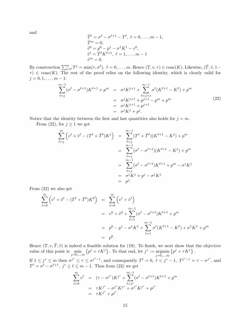
andT ` = σ` − σ`+1 − T `, ` = 0, . . . ,m− 1,Tm = 0,v0 = p0 − p1 − σ1K1 − v0,

v` = T `K`+1, ` = 1, . . . ,m− 1vm = 0.

By construction∑m

j=` Tj = min(τ, σ`), ` = 0, . . . ,m. Hence (T, v, τ) ∈ cone(K). Likewise, (T , v, 1−

τ) ∈ cone(K). The rest of the proof relies on the following identity, which is clearly valid forj = 0, 1, . . . ,m− 1:

m−1∑`=j

(σ` − σ`+1)K`+1 + pm = σjKj+1 +m−1∑`=j+1

σ`(K`+1 −K`) + pm

= σjKj+1 + pj+1 − pm + pm

= σjKj+1 + pj+1

= σjKj + pj .

(22)

Notice that the identity between the first and last quantities also holds for j = m.From (22), for j ≥ 1 we get

m∑`=j

(v` + v` − (T ` + T `)Kj

)=

m−1∑`=j

(T ` + T `)(K`+1 −Kj) + pm

=m−1∑`=j

(σ` − σ`+1)(K`+1 −Kj) + pm

=m−1∑`=j

(σ` − σ`+1)K`+1 + pm − σjKj

= σjKj + pj − σjKj

= pj .

From (22) we also getm∑`=0

(v` + v` − (T ` + T `)K0

)=

m∑`=0

(v` + v`

)= v0 + v0 +

m−1∑`=1

(σ` − σ`+1)K`+1 + pm

= p0 − p1 − σ1K1 +m−1∑`=1

σ`(K`+1 −K`) + σ1K1 + pm

= p0.

Hence (T, v, T , v) is indeed a feasible solution for (19). To finish, we next show that the objectivevalue of this point is min

j=0,...,m

{pj + τKj

}. To that end, let j∗ := argmin

j=0,...,m

{pj + τKj

}.

If 1 ≤ j∗ ≤ m then σj∗ ≤ τ ≤ σj

∗−1, and consequently T ` = 0, ` < j∗ − 1, T j∗−1 = τ − σj∗ , and

T ` = σ` − σ`+1, j∗ ≤ ` ≤ m− 1. Thus from (22) we getm∑`=0

v` = (τ − σj∗)Kj∗ +m−1∑`=j∗

(σ` − σ`+1)K`+1 + pm

= τKj∗ − σj∗Kj∗ + σj∗Kj∗ + pj

∗

= τKj∗ + pj∗.

15

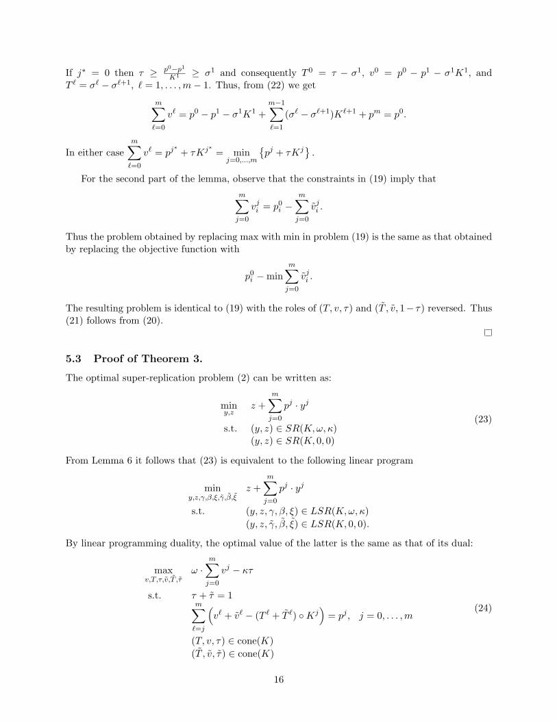
If j∗ = 0 then τ ≥ p0−p1

K1 ≥ σ1 and consequently T 0 = τ − σ1, v0 = p0 − p1 − σ1K1, andT ` = σ` − σ`+1, ` = 1, . . . ,m− 1. Thus, from (22) we get

m∑`=0

v` = p0 − p1 − σ1K1 +m−1∑`=1

(σ` − σ`+1)K`+1 + pm = p0.

In either casem∑`=0

v` = pj∗

+ τKj∗ = minj=0,...,m

{pj + τKj

}.

For the second part of the lemma, observe that the constraints in (19) imply that

m∑j=0

vji = p0i −

m∑j=0

vji .

Thus the problem obtained by replacing max with min in problem (19) is the same as that obtainedby replacing the objective function with

p0i −min

m∑j=0

vji .

The resulting problem is identical to (19) with the roles of (T, v, τ) and (T , v, 1− τ) reversed. Thus(21) follows from (20).

5.3 Proof of Theorem 3.

The optimal super-replication problem (2) can be written as:

miny,z

z +m∑j=0

pj · yj

s.t. (y, z) ∈ SR(K,ω, κ)(y, z) ∈ SR(K, 0, 0)

(23)

From Lemma 6 it follows that (23) is equivalent to the following linear program

miny,z,γ,β,ξ,γ,β,ξ

z +m∑j=0

pj · yj

s.t. (y, z, γ, β, ξ) ∈ LSR(K,ω, κ)(y, z, γ, β, ξ) ∈ LSR(K, 0, 0).

By linear programming duality, the optimal value of the latter is the same as that of its dual:

maxv,T,τ,v,T ,τ

ω ·m∑j=0

vj − κτ

s.t. τ + τ = 1m∑`=j

(v` + v` − (T ` + T `) ◦Kj

)= pj , j = 0, . . . ,m

(T, v, τ) ∈ cone(K)(T , v, τ) ∈ cone(K)

(24)

16

To finish, observe that for fixed τ ∈ [0, 1] the linear program (24) can be decoupled into n linearprograms, each one of the form (19) or (19) with min instead of max. The expression (5) for theoptimal value then follows from Lemma 11.

5.4 Proof of Theorem 5.

(a) From the definition of ji[τ ] and j′i[τ ] it follows that

ω · ν(τ) − τκ =n∑i=1

|ωi|pji[τ ]i +∑i∈I−

ωi(p0i −K

ji[τ ]i ) + τ

(n∑i=1

ωiKji[τ ]i − κ

)for τ ↓ τ , (25)

and

ω · ν(τ) − τκ =n∑i=1

|ωi|pj′i[τ ]i +

∑i∈I−

ωi(p0i −K

j′i[τ ]i ) + τ

(n∑i=1

ωiKj′i[τ ]i − κ

)for τ ↑ τ , (26)

Optimality of τ implies that the slope in (25) is non-positive and the slope in (26) is non-

negative. Thusn∑i=1

ωiKji[τ ]i ≤ κ ≤

n∑i=1

ωiKj′i[τ ]i and so there exists some λ ∈ [0, 1] such that

(7) holds. Using (7), (25) and (26), we obtain

ω ·ν(τ)−τκ =n∑i=1

(λ|ωi|pji[τ ]i + (1− λ)|ωi|p

j′i[τ ]i

)+∑i∈I−

ωi

(p0i − λK

j′i[τ ]i − (1− λ)Kji[τ ]

i

).

Thus the point z, yji given by (8) has objective value equal to (5). Therefore to finish it sufficesto show that it is feasible for (2). Indeed, since ωI+ ,−ωI− ≥ 0 and λ ∈ [0, 1], we have

m∑j=0

yj · (S −Kj)+ + z

=n∑i=1

|ωi|(λ(si −Kji[τ ]

i )+ + (1− λ)(si −Kj′i[τ ]i )+

)+∑i∈I−

ωisi −∑i∈I−

ωi

(λK

j′i[τ ]i + (1− λ)Kji[τ ]

i

)

≥

∑i∈I+

ωi

(si − λKji[τ ]

i − (1− λ)Kj′i[τ ]i

)+

+

−∑i∈I−

ωi

(si − λK

j′i[τ ]i − (1− λ)Kji[τ ]

i

)+

+∑i∈I−

ωi

(si − λK

j′i[τ ]i − (1− λ)Kji[τ ]

i

)≥ (ω · s− κ)+ .

Above the first inequality follows from a++b+ ≥ (a+b)+, the second from a++b+−b ≥ (a−b)+and (7).

(b,c) These follow via similar (but simpler) arguments to that in (a).

17

5.5 Proof of Theorem 7.

The optimal super-replication problem (10) can be written as:

minz,y,y+,y−

z +m∑j=0

(pj+ · yj+ − p

j− · y

j−)

s.t. (y, z) ∈ SR(K,ω, κ)(y, z) ∈ SR(K, 0, 0)y = y+ − y−y ∈ Rn×(m+1)

y+, y− ∈ Rn×(m+1)+ .

(27)

From Lemma 6 it follows that (27) is equivalent to the following linear program

minz,y,y+,y−γ,β,ξ,γ,β,ξ

z +m∑j=0

(pj+ · yj+ − p

j− · y

j−)

s.t. (y, z, γ, β, ξ) ∈ LSR(K,ω, κ)(y, z, γ, β, ξ) ∈ LSR(K, 0, 0)y = y+ − y−y ∈ Rn×(m+1)

y+, y− ∈ Rn×(m+1)+ .

6 Acknowledgements

We thank Hansen Chen at Susquehanna International Group for providing numerous insightfulcomments on a preliminary version of this manuscript. Luis Zuluaga’s research is supported byNSERC grant 290377.

References

[1] D. Bertsimas and I. Popescu. On the relation between option and stock prices: An optimizationapproach. Oper. Res., 50:358–374, 2002.

[2] P. Boyle and X. Lin. Bounds on contingent claims based on several assets. J. Fin. Econ.,46(3):383–400, 1997.

[3] A. d’Aspremont and L. El Ghaoui. Static arbitrage bounds on basket option prices. Math.Program. Series A, 106:467–489, 2006.

[4] M. H. Davis and D. Hobson. The range of trading option prices. Mathematical Finance,17(1):1–14, 2007.

[5] V. H. De la Pena, R. Ibragimov, and S. J. Jordan. Option bounds. J. Appl. Probab., 41A:145–156, 2004.

[6] C. Jabbour, J. Pena, J. Vera, and L. Zuluaga. An estimation-free, robust CVaR portfolioallocation model. Journal of Risk, forthcoming.

18

[7] S. Karlin and W. Studden. Tchebycheff Systems: with Applications in Analysis and Statistics.Pure and Applied Mathematics Vol. XV, A Series of Texts and Monographs. IntersciencePublishers, John Wiley and Sons, 1966.

[8] D. Hobson P. Laurence and T.H. Wang. Static arbitrage optimal subreplicating strategies forbasket options. Insurance Mathematics and Economics, 37:553–572, 2005.

[9] D. Hobson P. Laurence and T.H. Wang. Static arbitrage upper bounds for the prices of basketoptions. Quant. Financ., 5(4):329–342, 2005.

[10] W. Magrabe. The value of an option to exchange one asset for another. J. Finance, 3:177-186,1978.

[11] J. Pena, J. Vera, and L. Zuluaga. Static-arbitrage lower bounds on the prices of basket optionsvia linear programming. Technical report, Carnegie-Mellon University, Pittsburgh, 2007.

[12] J. Renegar. A Mathematical View of Interior-Point Methods in Convex Optimization, volume 3of MPS/SIAM Ser. Optim. SIAM, 2001.

[13] T. Rockafellar. Convex Analysis. Princeton University Press, Princeton, 1970.

[14] L. Zuluaga and J. Pena. A conic programming approach to generalized Tchebycheff inequali-ties. Math. Oper. Res., 30(2):369–388, 2005.

19

Table 1: CBOE data from May 17th, 2004 on June 2004 contracts expiring June 18. The table gives prices of call options traded (volumegreater than zero) on May 17th for the 30 stocks underlying the DJX index basket option. For every stock, the first row corresponds to the differentstrike prices, and the second and third rows correspond to the respective ask and bid prices. The entry of 0.00 for each stock gives the close priceof the stock, which can be considered as the forward option (call option with strike price zero) price.

0.00 20.00 22.50 25.00 27.50MSFT 25.79 5.70 3.20 1.15 0.20

25.42 5.50 3.10 1.05 0.150.00 25.00 27.50 30.00 32.50 35.00

AA 29.70 4.10 2.20 0.95 0.30 0.1528.60 3.90 2.05 0.85 0.20 0.050.00 65.00 70.00 75.00

AIG 70.15 5.40 2.10 0.4569.22 5.30 2.00 0.400.00 47.50 50.00

AXP 49.30 2.20 0.8048.20 2.05 0.700.00 40.00 42.50 45.00

BA 43.61 3.10 1.35 0.4042.49 2.90 1.25 0.300.00 35.00 37.50

VZ 36.74 1.50 0.4035.68 1.40 0.300.00 60.00 70.00 75.00 80.00 85.00

CAT 74.45 13.80 4.90 1.95 0.60 0.2072.70 13.60 4.80 1.90 0.50 0.100.00 40.00 42.50 45.00

DD 41.48 2.00 0.70 0.1541.01 1.80 0.55 0.100.00 20.00 22.50 25.00 27.50

DIS 22.99 3.00 1.05 0.20 0.1022.69 2.95 0.90 0.15 0.000.00 25.00 27.50 30.00 32.50 35.00 37.50

GE 30.06 5.10 2.70 0.85 0.15 0.05 0.0529.68 4.90 2.60 0.75 0.10 0.00 0.000.00 47.50 50.00 55.00 60.00 65.00 70.00

WMT 55.25 7.40 5.10 1.45 0.15 0.05 0.0554.14 7.20 4.90 1.30 0.10 0.00 0.000.00 35.00 40.00 42.50 45.00 47.50 50.00 55.00

GM 43.90 8.70 4.20 2.30 1.05 0.40 0.15 0.0542.88 8.60 4.00 2.20 0.95 0.30 0.10 0.000.00 30.00 32.50 35.00 37.50 40.00

HD 33.75 3.80 1.85 0.60 0.15 0.0533.07 3.60 1.70 0.55 0.10 0.000.00 30.00 32.50 35.00 37.50 40.00

HON 33.43 2.85 1.15 0.30 0.10 0.0532.44 2.70 1.00 0.20 0.00 0.000.00 15.00 17.50 20.00 22.50

HPQ 19.70 4.60 2.30 0.70 0.1519.21 4.50 2.20 0.65 0.100.00 80.00 85.00 90.00 95.00 100.00

IBM 86.03 6.30 2.65 0.70 0.20 0.0585.15 6.10 2.50 0.65 0.15 0.000.00 27.50 30.00 32.50 35.00 37.50 40.00 42.50 45.00

JPM 35.47 8.00 5.60 3.30 1.45 0.45 0.10 0.10 0.0534.75 7.80 5.40 3.10 1.35 0.35 0.05 0.00 0.000.00 47.50 50.00 55.00

KO 50.12 2.70 1.00 0.0549.51 2.55 0.85 0.000.00 40.00 42.50 45.00

XOM 43.54 3.40 1.45 0.4043.01 3.20 1.35 0.300.00 20.00 22.50 25.00 27.50 30.00

INTC 27.30 6.90 4.50 2.30 0.80 0.2026.44 6.80 4.30 2.25 0.70 0.100.00 50.00 55.00

JNJ 55.10 5.00 1.1054.13 4.80 1.050.00 80.00 85.00 90.00

UTX 82.80 3.60 1.20 0.3081.50 3.40 1.10 0.200.00 80.00 85.00 90.00

MMM 83.89 4.20 1.30 0.2582.75 4.00 1.15 0.150.00 45.00 47.50 50.00 55.00 60.00

MO 50.00 4.90 2.80 1.20 0.15 0.1048.50 4.70 2.65 1.15 0.10 0.000.00 45.00 47.50 50.00

MRK 46.89 2.15 0.70 0.1546.00 1.95 0.60 0.100.00 30.00 35.00 37.50 40.00 42.50

PFE 35.91 5.70 1.30 0.30 0.10 0.0535.00 5.50 1.20 0.25 0.05 0.000.00 90.00 95.00 100.00 105.00 110.00 115.00

PG 107.15 16.50 11.70 7.10 3.30 1.00 0.25105.81 16.30 11.40 6.90 3.10 0.90 0.200.00 25.00

SBC 24.49 0.4024.11 0.350.00 20.00 25.00 27.50 30.00

MCD 26.05 5.90 1.40 0.35 0.0525.50 5.80 1.30 0.25 0.050.00 30.00 35.00 40.00 42.50 45.00 47.50 50.00 55.00

C 45.30 15.00 10.00 5.20 3.00 1.30 0.40 0.15 0.0544.83 14.80 9.80 5.10 2.90 1.25 0.35 0.05 0.00

20

Table 2: Strike 80.00 DJX basket super-replicating strategy from LP formulation (eq. (11)). Optionprice upper bound = 19.8872. For every asset, the first row gives the strikes of the asset’s calloptions with a position greater than zero in the super-replicating strategy. The second row givesthe corresponding long position. In this particular experiment, the super-replicating portfolio doesnot contain any short positions.

22.50MSFT 0.071

25.00AA 0.071

65.00AIG 0.071

47.50AXP 0.071

40.00BA 0.071

35.00VZ 0.071

60.00CAT 0.071

0.00DD 0.071

20.00DIS 0.071

25.00GE 0.071

47.50WMT 0.071

35.00GM 0.071

30.00HD 0.071

30.00HON 0.071

15.00HPQ 0.071

80.00IBM 0.071

27.50JPM 0.071

47.50KO 0.071

40.00XOM 0.071

20.00INTC 0.071

50.00JNJ 0.071

0.00 80.00UTX 0.054 0.017

80.00MMM 0.071

45.00MO 0.071

45.00MRK 0.071

30.00PFE 0.071

90.00PG 0.071

0.00SBC 0.071

20.00MCD 0.071

35.00C 0.071

21

Table 3: Strike 80.00 DJX basket super-replicating strategy from LP formulation (eq. (11)) plusdiversification constraints (eq. (12)). Option price upper bound = 19.9022. For every asset, thefirst row gives the strikes of the asset’s call options with a position greater than zero in the super-replicating strategy. The second row gives the corresponding long position. In this particularexperiment, the super-replicating portfolio does not contain any short positions.

22.50MSFT 0.071

25.00AA 0.071

65.00AIG 0.071

47.50AXP 0.071

40.00BA 0.071

35.00VZ 0.071

60.00CAT 0.071

0.00DD 0.071

20.00DIS 0.071

25.00 35.00 37.50GE 0.071 0.011 0.025

47.50 65.00 70.00WMT 0.071 0.010 0.025

35.00 55.00GM 0.071 0.050

30.00 40.00HD 0.071 0.007

30.00 40.00HON 0.071 0.007

15.00HPQ 0.071

80.00 100.00IBM 0.071 0.007

27.50 45.00JPM 0.071 0.025

47.50 55.00KO 0.071 0.050

40.00XOM 0.071

20.00INTC 0.071

50.00JNJ 0.071

0.00 80.00UTX 0.054 0.017

80.00MMM 0.071

45.00MO 0.071

45.00MRK 0.071

30.00 42.50PFE 0.071 0.007

90.00PG 0.071

0.00SBC 0.071

20.00 30.00MCD 0.071 0.050

35.00 55.00C 0.071 0.025

22