antónio a. martins 1,*, paulo e. laranjeira carlos...
TRANSCRIPT
In: Progress in Porous Media Research ISBN: 978-1-60692-435-8 Editors: Kong Shuo Tian and He-Jing Shu © 2009 Nova Science Publishers, Inc.
Chapter 5
MODELING OF TRANSPORT PHENOMENA IN POROUS MEDIA USING NETWORK MODELS
António A. Martins 1,*, Paulo E. Laranjeira 2,†, Carlos Henrique Braga1,‡, Teresa M. Mata3,#
1 CEFT - Center for Transport Phenomena Studies 2 LSRE – Laboratory of Separation and Reaction Engineering
3 LEPAE – Laboratory for Process, Environmental and Energy Engineering Faculty of Engineering, University of Porto
Rua Dr. Roberto Frias S/N, 4200-465 Porto, Portugal
ABSTRACT
This article discusses the application of network models to represent the local structure of a packed bed, and their application in the modeling of a fluid flow and mass transport in a porous media. It is divided in two parts. Part A is a critical review of the network models available in literature, with a focus in the main modeling methodologies proposed, its advantages, the main assumptions and limitations. The analysis shows that the local geometrical structure of a porous media is the key factor that controls the observed macroscopic behavior. In Part B, and partly supported by the models described and the conclusions drawn in Part A, a bi-dimensional network model is proposed to describe fluid flow and mass transport in a packed bed and studied in detail. The network itself is made up of two types of elements, the chambers and channels, to better account for the void space variability. A geometrical model is proposed, able to determine the average values of the network elements size distributions. The flow modeling takes into accounting explicitly the relations between the two types of elements. Results show that only for that case it is possible to describe all the possible flow regimens in a porous medium. Good agreement with experimental data is obtained for the packed beds composed by nearly sized particles. The mass transport model was built on network and
* [email protected] † [email protected] ‡ [email protected] # [email protected]

António A. Martins, Paulo E. Laranjeira, Carlos Henrique Braga et al. 166
flow models and it is capable of varying the relative importance of the main transport mechanisms, convection and diffusion, by changing the characteristic geometrical dimensions of the network elements. Nevertheless, results also show that the mass transport can be affected by the flow regimen observed in the network.
Keywords: Network Models; Porous Media; Geometrical Modeling; Fluid Flow; Mass Transport; Dispersion.
INTRODUCTION
General Description of the Problem
In nature and in a large number of practical applications it is common to find porous
media. At a microscopic scale and in a general sense, virtually every solid material can be considered as being porous, with the exception of metallic structures, dense rocks and some plastics (Dullien, 1992). The existence of reliable models to predict the behavior of porous media and of the transport phenomena occurring inside them can be very important in many scientific and technological areas. Some examples are listed as follows (Kaviany, 1995; Sahimi, 1995).
• Chemical process engineering: fixed bed reactors, filtration, drying, trickle bed
reactors, chromatography, adsorption/desorption, ionic change, fuel cells, catalytic converters to reduce pollutant emissions from vehicles, absorption and distillation columns with and without chemical reaction.
• Environmental engineering: migration of contaminants in soil and ground water, irrigation, soils cleaning with vapor injection, and incineration.
• Natural’s reservoirs:natural gas and oil production, flow of water in mines. • Mechanical engineering: thermo insulation, combustion involving pyrolysis of
reactive or non reactive materials, tribology and lubrication, nuclear reactors with gas cooling, solidification or fusion of binary mixtures, dehumidification, sinterization and aggregation of particles by compression and heating.
• Civil construction: humidity penetration in porous materials and development of protection strategies to avoid their degradation by water diffusion through them, analysis of water retention in dams and flow throughout their bed.
The previous list does not intended by all means to be representative of all systems and
applications where porous medium are an important part, in many cases controlling the overall behavior and/or performance. Although other factors can also play an important role, the porous medium geometry, especially at the local/microscopic scale, is always an important aspect that any model trying to describe and predict their behavior has to consider explicitly.
For example, Comiti and Renaud (1989) compared the pressure drop in packed beds composed of spheres and particles with a parallelepiped shape (plates), determining the constants from the Ergun equation. It was observed that the lower the ratio between the

Modeling of Transport Phenomena in Porous Media Using Network Models 167
characteristic dimensions of the plates the larger the difference between the values of the constants proposed by MacDonal et al. (1979), based on data obtained mostly in packed bed of spheres, and the values determined experimentally. The authors explained these differences with the influence of the bed structure on the flow. As one can expect there is a tendency of the parallelepiped particles to align in the normal direction of the flow, thus making the fluid flow similar to flow of small jets of fluids between layers of particles, with the occurrence of major losses of kinetic energy and resulting in a larger pressure drop when compared to packed beds made of spherical particles.
Seguin et al. (1998a and 1998b) also studied the same type of packing with the purpose of analyzing the transition between flow regimens. The packing composed by plates were built with care in order to determine the influence of the flow direction in relation to the plates orientation. Both situations analyzed are presented in Figure 1.
Figure 1. Trajectory of a particle through two types of plates packed bed studied by Seguin et al. (1998a and 1996b): a) plates orientation perpendicular to the flow direction; b) plates orientation parallel to the flow direction.
Seguin et al. (1998a) have concluded that the transition between laminar and non-linear
regimens strongly depends on the relative direction of the flow in relation to the plates orientation. The authors explained this difference in behavior to the major packing anisotropy with more parallelepiped particles.
The previous examples make it clear that the utilization of the Ergun Equation to predict the pressure drop inside a particles packed bed can lead to large errors, making useless the design of process units based on the values obtained with those equations. Only through the inclusion of local packing characteristics it is possible to discriminate between both situations presented in Figure 1.
The complex nature of real porous media leads to the usage of a simplified representation of the porous structure, since only this way it is possible to describe the phenomenological behavior of the medium. The model selection is a function of the desired level of detail, the intended application, the porous medium characteristics, such as the porosity, the particles type (shape, dimensions and internal structure), the medium type (consolidated or not), among other relevant considerations.

António A. Martins, Paulo E. Laranjeira, Carlos Henrique Braga et al. 168
It is obvious that the price to pay for a high detailed packed bed description is the need to have a large quantity of information about the geometrical structure and its topology. In particular, the macroscopic behavior depends on the local behavior at the level of the particles that compose the porous medium (Melli et al., 1992). This way, any attempt to model it should be based on an adequate description of the local geometric and transport phenomena conditions. From this local description, a strategy to convert it to the macroscopic scale should be defined in a way to allow the determination of the macroscopic parameters such as the total pressure drop through the packed bed, the axial dispersion coefficient, among others. Also, more detailed models lead to more complex equations systems to describe their behavior, making it harder to solve them and demanding more extensive computational resources.
Nowadays, there is a strong pressure for the adoption of more energy efficient processes and consuming less raw-materials. Besides the obvious economic gains, they are more environmentally friend, with lower pollutant emissions. Just acquiring a more deep knowledge of the transport phenomena occurring in the interior of a porous media, it is possible to implement more adequate changes and more efficient processes can be developed. Thus, there is a need for more rigorous and accurate models to describe and/or predict the transport phenomena in a porous medium.
Darcy (1856) work concerning the water flow through a packed bed composed by sand particles is considered to be the starting point of the studies about transport phenomena through a porous media. This author has observed that the pressure drop through a particles bed is proportional to a volumetric flow rate. This proportionality relation is named as Darcy’s law. The proportionality constant depends on the fluid viscosity and on a parameter that varies with the porous media characteristics, called permeability, k . Despite this relation has been proposed from experimental data, it has been shown to be valid if the flow velocity is low, i.e. for laminar flow regimen (Whitaker, 1986).
Initially, the strategies for transport phenomena description in a porous media were empiric and based on experimental data (like the relationship proposed by Darcy) and were used to determine the values of the model constants. The results obtained were only valid to describe the behavior of the different types of porous media in which the experimental data were obtained. Despite these problems, the level of knowledge and the calculation capacity precluded the use of more rigorous strategies. Scheidegger (1960) presents some of the developed expressions, with the inclusion of their limitations.
To allow the mathematical and computational treatment of equations that describe the phenomena occurring in porous media, simplified models of the porous media structure are generally used. The conservation equations system reflect the influence of the various phases occurring in the porous media and its resolution allows one to describe the behavior of the media, without the need to use empirical parameters. The increase in rigor conducts to an increase in the level of complexity of the equations to be solved, requiring the use of numerical methods for the majority of the cases. The increase of the computational capabilities makes it possible to use models even more rigorous, using even more information about the media characteristics. In the next sections the main type of models proposed in literature are presented and discussed.

Modeling of Transport Phenomena in Porous Media Using Network Models 169
Model Characteristics for the Description of Transport Phenomena in Porous Media
The development of a model aiming to describe the local structure of a porous medium
should have the following characteristics: • To give a simplified description but at the same time reasonable, including all the
essential aspects of the porous media structure to be studied. The description of the transport phenomena is simplified, but should be satisfactory from a mathematical and physical point of view.
• To allow the calculation and prevision of the transport coefficients and other important parameters, from the morphological and physico-chemical characteristics of the porous matrix components.
More detail at the local level implies a higher complexity in the mathematical modeling,
making it sometimes extremely difficult to obtain the analytical solutions even for limit situations. In that case one needs to use numerical solutions to solve the balance equations and to obtain the parameters values. However, the use of more rigorous models at the local level presents several advantages.
• It allows for the optimization and effective control of the operation units where
porous medium is an important part. Operational problems can be quickly identified and corrected in an efficient manner, making it possible a preventive management of the process, detecting and correcting problems before they are significant.
• It allows the design of a unit without having to build pilot units to assure an adequate scale-up, with evident economic and time gains. Besides that, new packing structures can be studied and analyzed with a good degree of certainty, reducing the need to have specific experimental data and of time consuming determination.
In another hand, some conditions limit the development of a model, which should be
coherent and consistent, as well as physically valid and adequate to the situation under study. Its parameters should be easily determined from the medium characteristics and should possess a rigorous physical meaning. One should also pay attention to the computational limitations associated with the use of very complex and rigorous models, but prohibitive in terms of its implementation complexity and computational demands. The time needed to obtain the parameters values can also be determinant, in particular when one is interested in a fast analysis of the performance and the influence of the operating conditions in processes where porous media is a key part. One can further expect the reduction of these restrictions due to the progressive cost reduction and to the increase of computational capacities of the future hardware. Anyway currently there is still the need to use simplified models of the porous matrix structure.
It is possible to define two classes of models: one considering the medium as a continuum and the other that describes the local structure of the medium as a collection of discrete elements interconnected and interrelated with each other. For the continuum models the medium can be viewed as composed by just one phase with homogeneous characteristics. The characteristics of porous matrix are included in these models through the definition of average

António A. Martins, Paulo E. Laranjeira, Carlos Henrique Braga et al. 170
parameters (at macroscopic level). This strategy can be very useful, due to the large quantity of studies and available results in literature in the area of continuum mechanics, being the most common way to model fixed bed reactors (Froment and Bischoff, 1990). Despite of these advantages, this type of models do not allow an adequate description of anisotropic media or systems with strong variations of the structure at the local level.
The other class of models tries to describe the local behavior and from there obtain the macroscopic performance. Two variants exist. One in which it is assumed that the behavior of the porous media can be modeled by a fundamental cell with a structure representative of the local structure. The presence of other particles is taken into account through the boundary conditions applied at the cell surface (Brinkman, 1947; Happel, 1958 and 1959; Kuwabara, 1959; Hasimoto, 1959; Sangani and Acrivos, 1982a, 1982b and 1988; Zick and Homsy, 1982; Koch and Brady, 1985; Quintard and Whitaker, 1993). This type of model is called normally as cell models, and it is normally used to describe transport phenomena in packed beds, or porous media with large values of porosity. In the other variant, it is considered that the flow resistance is mainly controlled by the constrictions between the network elements (Van Brakel, 1975; Dullien, 1992), and that the interconnected nature of the porous media can be represented by constructing a network of elements. Thus, they are called network models in agreement with its real structure. In this type of models it is possible to use the real structure of the porous media, obtained for example through serial tomography methods, Nuclear Magnetic Resonance (NMR) image analysis, and tri-dimensional reconstruction (Gladden, 1993, 1994; Gladden et al., 1995; Mata et al., 2001a and 2001b). This is the optimum solution since there is no information loss during the model construction. However, there may be experimental difficulties associated to the medium void determination and the description of the solid-fluid boundary, and with the definition of the boundary conditions to the balance equations. In most cases the network simply use simple elements interconnected with each other in a manner simple enough to be able to characterize the behavior of the porous medium.
Albeit the restrictions presented above, some studies can be found in literature where the local structure of the porous media is used directly (Manz et al., 1999; Dwyer et al., 1999, Zeiser et al., 2001; Dixon et al, 2006). Even though good results were obtained by these authors, the computational capabilities and the ability of existing algorithms still limit the dimensions and flow conditions that can be studied and simulated.
Overview of this Article In this article we will focus our attention in the utilization of network models to describe
and model transport phenomena in porous media, with a focus to the characterization of the network local structure, flow field and mass transport/dispersion. In part A it is presented a review of the different network models currently available in literature, including a description of the different variants proposed and how the parameters needed to characterize the network elements can be determine and how networks models are used to describe the fluid flow and the mass transport inside a porous medium. Note that in this part we will focus our attention to the different methodologies for describing and simulating transport phenomena, thus no exhaustive listing of works where network models are used will be done here. In part B a hierarchical network model is described and used to describe the fluid flow

Modeling of Transport Phenomena in Porous Media Using Network Models 171
and the mass transport in a porous medium with a focus in packed beds. The model predictions were compared with experimental data and the behavior predicted using correlations available in literature to assess in which conditions the model is adequate to describe the flow and transport phenomena in packed beds.
PART A – REVISION OF NETWORK MODELS PROPOSED IN LITERATURE
NETWORK MODELS – TYPES AND CHARACTERIZATION
The distribution of the characteristic dimensions of the network of elements, their
geometric shape, and the way they are interconnected constitute the characteristics that define a network model. Generally, they can be classified according to their dimensionality, type of elements used and topological structure. The dimensionality represents the number of spatial dimensions taken into account in the modeling of transport phenomena in the porous medium. Accordingly to Van Brakel (1975) it is possible to have uni-, bi-, and tri-dimensional models, or even without any apparent dimension, having this author proposed a general classification of the large majority of models proposed in literature. In relation to the type of network model elements, these should be selected in order to simplify the analysis of the transport phenomena but at the same time with a geometrical form adequate to the porous medium under study. This way, the selection of the more adequate elements is more dependent on the porous medium and not so much on the dimensionality of the network models, and on the methodologies that can be used for its determination.
Uni-Dimensional Models Uni-dimensional capillaries networks can be viewed as networks of elements without
intersections. Because of its simplicity this was the first type of theoretical models to be proposed for the modeling of the porous media behavior, being the basis of the majority of correlations and equations currently used. Figure 2 shows some examples of this type of models. In many situations the structure of the porous medium is irregular justifying the definition of elements with a more complex, in particular with a flow variable section. Many times the selection of the elements geometry depends on the type of porous media that one wants to simulate (Petersen, 1958; Turner, 1958; Blick, 1966; Fedkiw and Newman, 1977; Azzam and Dullien 1977; Duda et al., 1983; Saéz et al., 1986; Sharma and Yortsos, 1987a; Skjtene et al., 1999). On a formal point of view, the description of transport phenomena at local level is now bi-dimensional, despite at the macroscopic level the behavior of the porous media is uni-dimensional.
Because a network of elements do not cross each other, the behavior of one element doesn’t influence the contiguous elements. For example, considering the mass transport through a uni-dimensional network model, no mass transport due to radial diffusion will

António A. Martins, Paulo E. Laranjeira, Carlos Henrique Braga et al. 172
occur, being the breakthrough curves just as a function of the values distribution of the capillaries velocity (Carbonell, 1979).
Figure 2. Examples of uni-dimensional capillaries network models.
Bi-Dimensional and Tri-Dimensional Models The description of many processes associated to porous media depends on the inclusion
of the natural interconnectivity of the porous medium, as for example in the analysis of the experimental results of the mercury porosimetry (Mata, 1998). Generally, models of this type can be described as networks composed by nodes interlinked among them through their branches, normally designed with pores, capillaries or channels. They can have any of the geometrical shapes considered for the uni-dimensional network of elements presented in Figure 2. The nodes may have or not physical existence, depending if a volume is attributed to them or not.
For the bi and tri-dimensional models one may define network models with a regular or irregular structure. Regular networks are those where it is possible to define a fundamental unit that by repetition can generate a network with the desired dimensions, or where it is possible to define an algorithm to generate the network structure that can be extended to the desired dimensions such as the Bethe networks (Sahimi, 1993a).
Several examples of bi-dimensional networks are presented in Figure 3. Besides a classification based on the different geometric shapes selected for each of the network elements, they can also be classified by the number of channels associated to each network node. This parameter is called the coordination number of the network. The more adequate value of the coordination number depends on the porous medium characteristics to be simulated. For the bi-dimensional networks presented, the coordination number can be constant and vary from 3=C (Chandler et al., 1982), 4=C (Koplik, 1982; Dias and Payatakes, 1986a and 1986b; Mann, 1991; Sorbie et al., 1991; Toledo et al., 1992), 6=C

Modeling of Transport Phenomena in Porous Media Using Network Models 173
and 3=C (Fatt, 1956) and 8=C (Fatt, 1956), or take diverse values in the same network, as it is the case of the networks utilized by Chatzis and Dullien (1977) where this parameter assumes values of two or four depending on the node position. For the majority of models one assumes that the distance between nodes is constant, despite some authors have concluded that this hypothesis may be not the most appropriate for some situations (Bryant and Blunt, 1993a).
Figure 3. Examples of regular models of bi-dimensional networks.
For most of networks presented in Figure 3 it is possible to define a fundamental element
from which a network of any dimension can be generated. For the Bethe network (Sahimi, 1995), the fractal structure of Adler (1994), or the branched structure of Andrade et al. (1998), the network is not generated by defining a fundamental block, but by a element in which it is define a recurrence relation. The networks utilized by Torelli and Scheidegger (1972) and Andrade et al. (1998) are similar but follows different branching schemes.
Non-regular bi-dimensional network models do not at least verify one of the two characteristics considered above, being some examples presented in Figure 3. It is possible to observe that some of these models can be considered as extensions of the regular bi-dimensional ones presented in Figure 4. For example the irregular model of Mann (1991) can

António A. Martins, Paulo E. Laranjeira, Carlos Henrique Braga et al. 174
be considered as an extension of the regular model, where the relative position between nodes and porous randomly change. In another hand, irregular models can be obtained by modifying the length of the channels between nodes, varying locally the coordination number on the regular networks, or modifying the local orientation of the network elements (Mann et al., 1986; Mann, 1991; Blunt and King, 1990; Ewing and Gupta, 1993; Sahimi, 1995). Other possibility of irregular bi-dimensional networks are models that have zones with very different characteristics, either concerning the coordination number of the nodes and also on their pores/channels density (Acuna and Yortsos, 1995). This last type of network models is applied mainly to fracture networks or two zone models.
Figure 4. Examples of irregular models of bi-dimensional networks.
Tri-dimensional network models can be considered as extensions of the bi-dimensional
models, where the network nodes are linked with each other in three dimensions. Similarly to the bi-dimensional network models, the tri-dimensional networks can be regular or irregular.
Figure 5 presents some examples of the regular and irregular tri-dimensional network models proposed in literature. The models of Friedman and Seaton (1996) and Rieckmann and Keil (1997) are typical examples of tri-dimensional network models with constant coordination number , differing only in the way the nodes are interlinked among them. Sherwood (1993), Ionnanidis and Chatzis (1993) considered regular tri-dimensional network models with a simple cubic regular structure, where the elements shows a rectangular shape, a more convenient geometrical shape for example to model consolidated porous media or porous media with fractures.
Also, it is possible to define other fractal structures, for example the Sierpinski Gasket, defined from a cubic solid and a specified recurrence relation (Adler, 1994). Irregular network models can be obtained from regular models, through for example varying the coordination number of the network nodes (Friedman and Seaton, 1996), or by imposing a

Modeling of Transport Phenomena in Porous Media Using Network Models 175
irregular structure, where the network elements can take any position. Other possibilities to generate irregular tri-dimensional network models can be found in literature (Hollewand and Gladden, 1992; Blunt and Bryant, 1990).
Figure 5. Examples of tri-dimensional models of: (a) regular and (b) irregular networks.
Other Models that May Be Considered as Network Models On the description and modeling of the mass transport through a porous media, in
particular through packed beds, it is common to use models of mixed tanks. Figure 6 shows some examples of this type of models. On their initial form these models try to describe only the flow mixture through a porous medium and to measure the deviation of the real flow conditions from plug flow (Fogler, 1992). The structure is equivalent to a uni-dimensional network model, where the influence of the links between the perfectly mixed tanks is normally neglected. In this type of models the links or branches do not influence the porous medium behavior.

António A. Martins, Paulo E. Laranjeira, Carlos Henrique Braga et al. 176
Figure 6. Examples of models of perfectly mixed tanks. Extensions to two dimensional structures were also proposed in literature. Schnitzlein and
Hofmann (1987) proposed a model of mixing tanks where the influence of the links is taken into consideration explicitly, being this model equivalent to a bi-dimensional network model with a coordination number equal to three. Schnitzlein and Hofmann (1987) analyzed the way to apply this model to a fixed bed reactor, having paid special attention to the adequate modeling of the zone closed to the wall. Villermaux and Schweich (1992) and Russel and LeVan (1997) proposed the use of mixed tanks model with a fractal structure, being presented two examples of it in Figure 6.
DTP and Geometrical Characteristics of the Network Elements In addition to the geometric structure and the way that the different network of elements
are associated with each other, other features should be defined, in particular the elements shape and their characteristic dimensions. The different possibilities proposed in literature are presented below, together with how the pertinent parameters values can be obtained from experimental data or computer simulations.
On the majority of the works it is assumed that the volume of nodes is negligible in relation to the branches volume. In some works this hypothesis has been relaxed (Ionnanidis and Chatzis, 1993; Thauvin and Mohanty, 1998; Wang et al., 1999b). In many cases the void volume of a porous medium is associated to the voids that correspond to nodes and not to branches (Berkowitz and Ewing, 1998). To include the node volumes, some authors defined additional zones in their ends. This way the network of elements will have parts with different geometric characteristics, akin to constrictions and expansions (Dias and Payatakes, 1986a; Constantinides and Payatakes, 1989). In practical terms any of the elements presented in Figure 6 may serve as a basis to a network model where one considers the existence of more

Modeling of Transport Phenomena in Porous Media Using Network Models 177
than one type of elements in the porous medium. Some works used approaches considering different elements for the nodes as well as to the branches (Ionnanidis and Chatzis, 1993; Thauvin and Mohanty, 1998; Wang et al., 1999b). However, the network generation and the modeling of flow is more complex for those models due to the presence of more than one type of element.
Except for some situations where the geometric characteristics of the porous medium are defined as a result of a controlled generation process, such as monolith structure as used in automotive catalysts (Irandoust and Anderson, 1988), the structure of a porous medium possess an irregular local structure, with local variations of the characteristics dimensions of the elements that constitute it. Statistical distributions is a good strategy to account for that variability. The parameters that define them can be inferred or determined from experimental data, obtained for example by mercury porosimetry or by image analysis. The adequate type of distribution function depends on the local structure and on the way the porous medium was generated. For packed beds, if the size distribution of the particles has a low standard deviation and they are almost spherical, the experimental and simulation results show that the size distribution of pores is approximately Gaussian with a low standard deviation (Nolan and Kavanagh, 1994; Rouault and Assouline, 1998). For consolidated porous media of packed beds formed by irregular particles or having a large distribution of the characteristic dimensions, the pore size distribution my be very large and could have more that one maximum (Dullien and Dhawan, 1975; Loh and Wang, 1995). In general it is not possible to define rules that allow one to know what is the most adequate porous size distribution for a certain porous medium, from their characteristics and constitutive elements (e.g. particles). In the large majority of the works typical distribution functions are used, with simple and well known mathematical description. Some examples are listed bellow.
• Uniform distributions, i.e. any size that have equal probability of occurring
(Petropoulos et al., 1989; Nicholson et al., 1988). • Punctual distributions (Sahimi, 1993b). In this type of distributions it is assumed that
the characteristic dimensions of the network elements only can take certain values. • Gaussian distributions are a common choice, since it is easy to determine their
parameters from experimental data (Nicholson and Petropoulos, 1968 and 1971). This type of distribution do not allow the inclusion of tails present on the pore size distributions, and give a non-null probability for the existence of channels with characteristic dimensions below zero. This last problem is solved truncating the normal distribution (Constantinides and Payatakes, 1989), or using a log-normal distribution that only can take positive values (Hampton et al., 1993; Zhang and Seaton, 1994; Suchomel et al., 1998a).
• Other distributions as for example: Chi-square, 2ℵ distribution (Nicholson and Petropoulos, 1968), triangular distributions (Nicholson and Petropoulos, 1973; Nicholson et al., 1988), Rayleigh distribution (Avilés and LeVan, 1991; Deepak and Bhatia, 1994), Weibull distribution (Ioannidis and Chatzis, 1993), truncated exponential distribution (Novakowski and Bogan, 1999), Haring and Greenkorn distribution (Haring and Greenkorn, 1970; Sorbie et al., 1989), among others.
António A. Martins, Paulo E. Laranjeira, Carlos Henrique Braga et al. 178
Some authors used directly the experimental porous size distribution. Imdakm and Sahimi (1987 and 1991), and Rege and Fogler (1987) used the experimental distributions obtained using mercury porosimetry techniques or image analysis. From a formal point of view, the use of distributions obtained from experimental data appears to be a better option than to assume an analytic distribution function. Due to the existence of equipment available and specifically designed to the determination of pore size distributions by mercury porosimetry (Mata et al. 2001a and 2001b), this is the preferred method to determined network pore size distribution (Loh and Wang, 1995, Matthews et al., 1995). Methods involving the water penetration in a porous medium were also considered by Payatakes et al. (1973a) and Marmur and Cohen (1997), being them formally similar to pore porosimetry.
The definition of more than one type of network elements requires the definition of more than one distribution, one for each elements type. It is common to assume the same type of probability density function for the characteristic dimensions of each network element (Loh and Wang, 1995; Wang et al., 1999b). However, in most cases the quantity and quality of experimental data do not allow the calculation of so many parameters without losing statistical significance.
Dullien (1992) recommends the combination experimental data obtained using mercury porosimetry and stereology or image treatment of the porous medium to the determination of pore size distributions. This last technique allows one to determine the network structure associated to a porous medium through the analysis of bi-dimensional cuts done on the porous medium. The cuts can be done by impregnating the medium under analysis with a resin (Mata, 1998; Liang et al., 2000; Vogel and Roth, 2000), or with a metallic league of low fusion temperature to stabilize the sample and facilitate its analysis (Dullien, 1991). Then, several cuts are done sequentially on the sample, being the sections obtained polished to improve the image capture and processing (Mata, 1998; Mata et al., 2001a and 2001b, Tsakiroglou and Payatakes, 2000). Analyzing several sections it is possible to create a representation of the network and how the branches and nodes are interrelated, having different techniques being proposed in literature for this purpose (Quiblier, 1984; Adler and Thovert, 1998; Liang et al., 2000; Vogel and Roth, 2000).
The determination of the structure and of the characteristic size distributions of the network corresponding to a packed bed can be done through its computational construction, followed by the analysis of the local geometrical structure. Generally, one first defines the type of container in the interior of which the particles will be deposited, followed by the type of particles and the deposition itself (Chan and Ng, 1986, 1987 and 1988; Chu and Ng, 1989a; Tassopoulos and Rosner (1992); Spedding and Spencer, 1995; Thompson and Fogler, 1997, Pilotti, 1998). Some authors only define the type of the particles deposition surface, neglecting the wall effects in the generation of the packed bed (Tassopoulos and Rosner, 1992). Yet, independently of the strategy utilized for the network generation, highly irregular structure are obtained, as shown in Figure 7.
Different authors studied various aspects, such as the influence of the presence of walls (Chan and Ng, 1987), and the particles characteristic size and shape distribution (Nolan and Kavanagh, 1995a; Coelho et al., 1997; Adler and Thovert, 1998; Jia and Williams, 2001).

Modeling of Transport Phenomena in Porous Media Using Network Models 179
Figure 7. Example of a packed bed formed by spherical particles with a size distribution.
To determine the equivalent network of the packed bed, the position of the centers of the
packed bed particles must be known and a structure for the equivalent network must be assumed. Chu and Ng (1989), Bryant and Blunt (1992) and Bryant et al. (1993a and 1993b) assumed that a packed bed can be described by tetrahedrons composed by four contiguous spheres, corresponding the vertices of the tetrahedrons to the spheres centers. Assuming that each tetrahedron possess a chamber and four capillaries, one for each one of the tetrahedron faces, after determining the network of tetrahedrons corresponding to the packed bed structure, the determination of the equivalent network is simple. Chu and Ng (1989a) proposed the use of pentahedrons in the zone more closed to the wall, in which it is not possible the definition of tetrahedrons due to the irregular structure of the spheres in that zone. Other ways to determine the local structure and the characteristic dimensions of the network elements are proposed in literature (Nolan and Kavanagh, 1994; Assouline and Rouault, 1997; Rouault and Assouline, 1998).
Other techniques are suggested in literature for the determination of the pore size distribution. One of the most promising is the application of nuclear magnetic resonance (NMR) for the characterization of the porous space (Gallegos and Smith, 1988; Gladden, 1993 and 1994; Latour et al., 1995; Gladden et al., 1995; Rigby and Gladden, 1996; Sederman et al., 1997 and 1998; Manz et al., 1999; Song, 2000). With this technique one can directly obtain the local structure of the porous medium, allowing its utilization for the simulation of the transport phenomena in porous media. This technique may be coupled with other methodologies, such as for example mercury porosimetry or nitrogen adsorption, allowing one to obtain other relevant information for the characterization of the local structure of a porous media (Rigby, 2000). The determination of the characteristic size distribution of a porous media do not allow one to infer which structure is more adequate to the equivalent network model, namely in which refers the coordination number or the way the elements positioned themselves in space, or what are the more adequate shapes for them. This
António A. Martins, Paulo E. Laranjeira, Carlos Henrique Braga et al. 180
type of information can only be obtained from the direct analysis of the local structure of the porous medium that is only possible using image analysis (Mata, 1998) or NMR (Manz et al., 1999) techniques. In packed beds generated on computer, the distribution function of the nodes coordination number can be easily obtained from the analysis of the network equivalent to the porous medium structure. Due to the difficulties associated with the determination of this distribution, it is common to assume a constant value of the coordination number in the network model.
FLUID FLOW MODELING
General Description With the exception of some transport phenomena, such as mass diffusion or heat transfer
by conduction through the solid phase, it is not possible to analyze the behavior of a porous medium without first describe the flow through it. One of the most important examples that is analyzed in detail in this paper is the mass transport through a porous media.
Experimental studies performed by Kim (1985), Fand et al. (1987), Kececioglu and Jiang (1994), Lage et al. (1997) and many other authors show that there are more than one flow regimen. The experimental data representation is generally done using dimensionless groups, as for example using a drag factor, F , as a function of the Reynolds number, Re , as shown in Figure 8 (Fand et al., 1987). The dimensionless parameters are defined in the form
2T
P
X
T
vD
LPF
ρΔ
= (1)
μρ PT Dv
Re = (2)
where TPΔ is the pressure drop through a porous medium, PD is the equivalent diameter of
particles, Tv is the superficial velocity, XL is the length of the medium according to the main flow direction, and ρ and μ represent the density and the fluid viscosity, respectively. From Figure 8 it is possible to conclude that depending on the Reynolds number value different flow regimens can be defined.
For low values of Re the flow is non-linear. Since the fluid velocity is very low, the influence of adsorption phenomena in the solid-liquid interface or molecular diffusion are dominant, being the flow modeling complex (Fand et al., 1987). This flow regimen is not normally found in practice.

Modeling of Transport Phenomena in Porous Media Using Network Models 181
Figure 8. Flow regimens in a porous medium (Fand et al., 1987).
The second and third flow regimens correspond to the situation where the flow at local
level is laminar. Despite the behavior on the third zone is non-linear, the available experimental results for the hydrodynamic behavior of the fluid at the level of the porous medium elements do not show the irregular behavior typical of turbulent regimen (Mickley et al., 1965; Dybbs and Edwards, 1984). In this zone the effects of the inertial and viscous effect in the flow are of some order of magnitude, being the inertial effects the result of the local and spatial variations of void space at the local level (Trussel and Chang, 1999). In order to differentiate both zones, some authors call to the second zone Darcy regimen and the third zone Forchheimer regimen (Fand et al., 1987).
Dybbs and Edwards (1984) explain the occurrence of a inertial flow regimen for Re values corresponding to laminar flow as a consequence of the incomplete development of the flow in the interior of the porous medium. Assuming that the internal structure of the porous medium can be seen as a network of capillaries, Dybbs and Edwards (1984) showed that a ratio near the unity between the length and the diameter of the channels allows a better fit of the experimental data. This way these authors argue that even for laminar flow conditions it is necessary to take into consideration the entrances and exits of the capillaries.
Other authors attributed the deviations from linear flow to the irregular structure of the porous medium. In particular for packed beds, the contractions and expansions occurring on its interior contribute to the existence of recirculation, and of non-linear flow zones (Payatakes et al., 1973a; Mei and Auriault, 1991). Fand et al. (1987) justified the existence of a transition zone between linear and non-linear regimen considering that the flow in the packed bed is similar to the flow around an isolated sphere. The analysis of the experimental results obtained with different particles distributions showed that the transition between flow regimens depends on the local characteristics of the medium. The turbulent regimen occurs for values of 310>Re , not being possible to define an universal value since this is a

António A. Martins, Paulo E. Laranjeira, Carlos Henrique Braga et al. 182
function of the packed bed structure, of the particle characteristic dimensions distributions, flow conditions and even of the fluids properties(Bear, 1972). The fourth zone corresponds to the turbulent flow, despite with characteristics different from the turbulence in tubes due to the irregular structure of the solid matrix and spatial limitations for the development of turbulence (Lage et al., 1997). If the F values as function of Re were represented in logarithmic scales, one would observe a linear dependence in this zone, analogue to the one observed for the fluid flow in rough cylindrical tubes.
Conduit Models One of the first type of models that tried to include, in a very crude way, the tube like
nature of the local packing structure are the so called conduit models (Carman, 1937). Although they may be considered as pure phenomenological models, they rely on the definition of an equivalent hydraulic diameter of a tube function of the porous medium characteristics, and therefore can be classified as simple uni-dimensional network models, as the conduits do not cross each other.
Laminar Flow
Relating the void volume and the superficial area of the porous with the definition of the
hydraulic diameter (Bird, 1960), and assuming laminar flow the following expression for the permeability is obtained
( )2
2
32
0
22
11616 Pkk
hh Dkk
dkTdk
εεεε−
=== (3)
where ( )20 1 Tkkk = is the Carman-Kozeny constant, T is the porous medium tortuosity
that accounts for the irregular structure of the conduits, and 0k is a constant function of the
conduits assumed to form the porous medium. For circular capillaries 0k =2, and its value varies between 2 and 2.5 for other geometries (Happel and Brenner, 1983; Liu et al., 1994). Based on experimental data, ( ) 521 .T ≈ , thus the normally called the Carman-Kozeny equation is obtained
( )2
2
3
1180 pDkε
ε−
= (4)
Carman (1937) assumed that 5=kk was a universal constant and independent of the
porous medium characteristics. However, experimental data showed that the value of this constant depends on the porosity and shape of particles (Coulson, 1948; Wyllie and Gregory,

Modeling of Transport Phenomena in Porous Media Using Network Models 183
1955). For packed beds made up of spheres, 5≈kk , for porosity values around 0.4 (Fand et al., 1987).
In terms of a friction factor, the Blake-Kozeny equation can be written in the form
( )3
21Re180
εε−
=Pf (5)
The previous expression is similar to empirical correlations presented in literature,
although they normally have different dependences on the porosity (Rumpf and Gupte, 1971; Agarwal and O’Neill, 1988; Ziólkoskwa and Ziokolwski, 1988; Dullien, 1992). However, those expressions are empiric and strictly valid for the porous media where the experimental data were obtained.
Also, the Carman-Kozeny has limited application when the packing is formed by particles with a large size distribution. MacDonald et al. (1991) has proposed the following expression,
( )
2
1
22
3
11801
⎟⎟⎠
⎞⎜⎜⎝
⎛
−=
XXk
εε
(6)
where 2X and 2X are the first and the second moments of the particle size distribution, and have observed a good agreement for the laminar flow in packed beds.
Liu and Masliyah (1996) also considered the basic Blake-Kozeny and tried to extend its validity. Assuming an isotropic medium, and analyzing the dependence of the interstitial velocity with the media local structure, these authors argue that the pressure drop in laminar regimen can be expressed in the form
( )T
P
vDk
Lp
3112
21 136
εεμ −
=Δ
− (7)
where 1k is a constant analogous to the Carman-Kozeny constant, kk . The porosity dependence is different from the one obtained before, but agrees with the dependence inferred by MacDonald et al. (1979) from experimental data. Turbulent Flow
The analysis made for laminar flow can also be extended for turbulent flow (Bird et al., 1960). Equating the pressure drop per unit length with the friction factor Pf , the following expression can be written
PT
hX
fvdL
P 4211 2
⎟⎠⎞
⎜⎝⎛=
Δε
ρ (8)
António A. Martins, Paulo E. Laranjeira, Carlos Henrique Braga et al. 184
Applying the definition of hydraulic diameter, and knowing that the experimental data suggests that 536 .fP ≈ , the previous expression can be written in the form
32 11751
εερ −
=Δ
TPX
vD
.L
P (9)
or using a friction factor in the form also known as the Burke-Plummer Equation
3
18750ε
ε−= .f P (10)
Comparing the expressions obtained for laminar and turbulent flow a different porosity
dependence is observed. These results are directly obtained from the analogy used, since for turbulent flow regimen the friction factor of the flow in a tube is constant, thus limiting the applicability of this equation to completed developed turbulent flow.
Ergun Equation and Extensions
The Blake-Kozeny and Burk-Plummer equations are only valid for the limit regimens of
the flow, where either friction or inertial forces are dominant. For the intermediate regimen, Ergun (1952) assumed that the total pressure of the flow through a porous medium is the sum of the values predicted by the two limit expressions, in the form
( ) 233
2
2
11T
PT
PX
T vD
BvD
ALP
εερ
εεμ −
+−
=Δ
(11)
where A and B are two constants that can be calculated from experimental data. Ergun (1952) obtained initially 150=A and 751.B = . Later, using a larger database, MacDonald et al. (1979) obtained 180=A , and 801.B = for smooth particles and 004.B = for rough particles. Even though these constants are considered to be universal, large deviations between predicted and experimental values may occur, especially for packings made up with particles with irregular shapes (Comiti and Renaud, 1989). Even for packings formed by spherical particles with narrow particle size distribution the differences can be relevant. For example the constant values obtained by Kim (1985) and Kececioglu and Jiang (1994) are in agreement with the recommendations of MacDonald et al. (1979), yet the experimental data of Rumpf and Gupte (1971) and Comiti and Renaud (1989) are better described using the values of A and B suggested by Ergun (1952). In many cases the determination of the constants from experimental data is the correct approach.
Defining the following dimensionless parameters
( )ερε−
Δ=
12
3
TX
PT*
vLDPF (12)

Modeling of Transport Phenomena in Porous Media Using Network Models 185
( )εμρ
−=
1Re PT* Dv
(13)
where *F is a equivalent friction factor and *Re a generalized Reynolds number, the MacDonal Equation can be written in the form
BAF ** +=
Re (14)
Experimental data presented in this form in logarithmic coordinates gives two
asymptotes. One with a slope -1 for low values of *Re that corresponds to laminar regimen. To high values of *Re , where the flow is turbulent a constant value is obtained equal to B . In literature other ways of presenting the experimental data were proposed, based on different definitions of the friction factor (Ergun, 1952), or using other methods to define the characteristic dimension such as the square root of the permeability (Ward, 1969; Kececioglu and Jiang, 1994), among others possibilities (Ahmed and Sunada, 1969; Ziólkoskwa and Ziólkowski, 1988; Venkataraman and Rao, 1998; Trussel and Chang, 1999).
The analysis Liu et al. (1994) and Liu and Masliyah (1996, 1999) was also extended to turbulent and the full range of flow regimens, but considering a different porosity dependence and definitions of the relevant dimensionless numbers, the friction factor and the Reynolds number. Comiti and Renaud (1989) tried to extend the validity of the MacDonald equation to packings with particles with shapes not spherical, with the explicit inclusion of the tortuosity, and superficial area of the particles. These authors have proposed the following expression (Mauret and Renaud, 1997)
( ) 2333
2
22 11
2112 TvdTvdM
X
T vaT
fvT
aLP
εερ
εεμγ −
+−
=Δ
(15)
where Mγ is a geometrical factor dependent of the packing local structure, vda is the particle
specific superficial area and 096802 .f = . The values of T and Vda are determined from experimental data obtained for packings made up of the particles of interest.
Uni-Dimensional Models The models described in the previous subsection may be loosely considered as network
models, because they assume that the local structure of a porous media is a bundle of tubes. However, as they do not try to describe the behavior of the individual elements, but use an analogy with the hydraulic diameter, they were considered separately.
The simplest uni-dimensional model is the bundle of parallel capillaries. Assuming that all capillaries have the same diameter for laminar regimen the following expression for the permeability is obtained

António A. Martins, Paulo E. Laranjeira, Carlos Henrique Braga et al. 186
32
2cd
kε
= (16)
The previous expression assumes that there is only one possible diameter value, and the
tubes are straight. However, Scheidegger (1960) showed that the dependence of the permeability on the porosity does not change with the inclusion of a pore size distribution. For describing situations where the flow is uni-dimensional, Scheidegger (1960) suggests to substitute the constant 32 of the denominator by a correction parameter sα , which value equals to 32 and 64 for uni-dimensional and bi-dimensional flows respectively.
The previous model does not account for the variations of the local structure of the porous media, equivalent to contractions and expansions that may have a profound impact in the behavior observed at the macroscopic scale. Many of the models and possible geometries are presented in Figure 2. However, a more accurate description of the local structure leads to a more complex description of the flow field, and in many cases the need to use numerical methods.
Petersen (1958) and Houpert (1959) were the first authors to consider models with capillaries having a variable section, in particular spatially periodic. Assuming that the flow inside the channels is similar to the flow in an orifice these authors showed that a quadratic equation similar to the Ergun Equation was obtained, but with the advantage that the values of parameters can be obtained directly from the geometrical characteristics of the channels. Blick (1966) and Niven (2002) reached similar conclusions using tubes with orifice constrictions inside the channels.
Other authors considered different channel geometries. Azzam and Dullien (1977), Ruth and Ma (1993) and Cao and Kitanidis (1998) considered circular channels with sudden changes in the radius. The computation of the flow field shows that for laminar regimen the pressure drop is a function of the constriction diameters. The transition between linear and non-linear flow regimens is smooth, depending on the geometrical characteristics of the channels, and occurs for Reynolds number much lower than those observed for straight tubes. These results are in qualitative agreement with the behavior observed in porous media, in particular in the transition zone.
However, in a real porous medium such as a packed bed, it is not expected to have abrupt variations in the characteristics dimensions of their elements. Thus, several models were proposed in literature where the channels radius varies in a continuous fashion. Pendse et al. (1983) analyzed and compared the relative merits of some of the alternatives available in literature.
Payatakes et al. (1973a, 1973b) have considered tubes where their radius varies according to a quadratic function. These authors also developed a geometrical model able to describe the local structure of the porous medium and to obtain the parameters of the quadratic function from experimental data. Results of this model compared well with experimental data for laminar and transition flow regimens. Sáez et al. (1986) considered the same radius variation, but to model the channels in a packed bed having a cubic regular structure. The computational and analytical study leads to the prediction of values for the constant A of the MacDonald Equation in agreement with other theoretical and experimental studies.

Modeling of Transport Phenomena in Porous Media Using Network Models 187
Fedkiw and Newman (1977), Neira and Payatakes (1979), Tilton and Payatakes (1984), Hemmat and Borhan (1995) and Cao and Kitanidis (1998), studied the case in which the radius varies in a sinusoidal form. These authors concluded that the onset on nonlinearities on the flow is due to the formation of recirculation areas in the channels, in particular after the constrictions, depending on the geometrical characteristics of the channels. Also, the results show that for laminar regimen the velocity profile tends to the Poiseuille profile and the constrictions are the aspect controlling the pressure drop in the porous medium. Deiber and Schowalter (1979) and Lahbabi and Chang (1986) studied the transition between flow regimens in channels with sinusoidal walls and showed that the inertial effects are relevant even though not visible at the macroscopic level. The predicted values of the Reynolds number for the transition agrees well with experimental data.
Channels that vary according to a hyperbolic function were considered by other authors (Venkatesan and Rajagoplan, 1980; Saeger et al., 1995; Thompson and Fogler, 1997). When compared with other models the predictions are very similar, showing that the form of the channels is not a determining factor. By comparison with the Carman-Kozeny equation, Pendse et al. (1983) concluded that sinusoidal channels are more adequate to describe the behavior of real porous media.
For laminar regimen, Sheffield and Metzner (1976) have proposed a different approach to calculate the pressure drop inside the channels, based on the lubrification theory. Assuming parallel and laminar flow, the pressure in an infinitesimal segment of the channel is given by the expression
4cdq
xP- ∝
∂∂
(17)
where q and cd represent respectively the volumetric flow rate and the characteristic
dimension of the network element. For a cylindrical tube with constant cd the proportionality
constant is equal to π128 . If cd is a smooth function of the length inside the channel, integrating the previous equation for a representative section of the channel leads to
( )∫=Δpl
cp xd
dxqcP0
4 (18)
where pc is a proportionality constant dependent on the channel geometrical characteristics.
Dias and Payatakes (1986a) used this approach assuming a channel made up of a central circular and sinusoidal on the extremes. Larson and Hidgon (1989) also used it to model the flow in a packed bed of spheres with a cubic structure where the particles are partially fused together. Results showed that the lubrification theory is valid when the porosity value is low, or the resistance to the flow is controlled by the constrictions between the particles. Similar conclusions were obtained by Hemmat and Borhan (1995), having these authors suggested ways of improving the validity of this approach.

António A. Martins, Paulo E. Laranjeira, Carlos Henrique Braga et al. 188
Bi-Dimensional/Tri-Dimensional Models The models described in the previous sections do not consider the interconnected nature
of the most real porous media. Bi-dimensional and tri-dimensional network models are used to consider those effects explicitly. However, when modeling the fluid flow inside the network of elements it is necessary to describe not only the behavior of the individual elements but also how they interact with each other.
The most relevant changes in relation with the uni-dimensional models is the need to write the mass balance equations to mixing nodes, and possibly expressions to describe the influence on the flow or the interconnection between different network elements. To simplify the description of the flow, many studies assume that the mixing nodes have a negligible influence on the flow, either because it is assumed that they have a negligible volume (Sahimi, 1995), or because their effects are incorporated in the channels (Dias and Payatakes, 1986a and 1986b). However, some examples can be found in literature where the two types of elements were considered explicitly and modeled separately (Koplik, 1982; Thauvin and Mohanty, 1998; Wang et al., 1999b).
The first practical application of a network model to describe the fluid flow in a porous media was the work of Fatt (1956) where a bi-dimensional model was used to study biphasic flow in a consolidated porous medium. Since then many more models were proposed in literature, with different strategies to solve the system of balance equations that describes the behavior of the network. The more common is based on the analogy between the flow in the network and the electrical current in a pure resistive circuit, almost always assuming steady state conditions and perfect mixing in the nodes. Considering that the absolute pressure in the nodes and the flow rate in the channels are analogous to the electrical potential and the intensity of the current respectively (Shearer et al., 1967; Palm, 1983), applying the Kirchoff laws to the equivalent electrical network it is possible to use efficient strategies developed for the analysis of circuits (Desoer and Kuh, 1969).
Other strategy is based on the Hady-Cross method to determine the flow rates in flow systems (Hampton et al., 1993). This method is iterative and involves the consecutive solution of a linear system of equations, only using the mass balance equations at the network nodes, but requires an initial estimative of the flow rates in the channels that for highly irregular networks may be difficult to obtain.
If the network is spatially periodic, Adler and Brenner (1985a and 1985b) have proposed a different methodology to model the fluid flow. These authors showed that the description of the flow can be reduced to the study of a fundamental cell, from which the behavior of a network with any dimensions can be obtained. Both linear and nonlinear flow regimens can be studied for these types of networks, and analytical expressions for the network permeability can be obtained using this method.
Whichever methodology is used it is always necessary to characterize the individual behavior of the network individual elements. To simplify the calculations, it is usually assumed that the tubes are cylindrical, although any other shape can be used. The popularity of the analogy with an electrical circuit stems from the fact that if the flow is laminar and the fluid Newtonian the resulting equation systems are linear, symmetric and positive definite, allowing the use of efficient numerical methods to obtain its solution (Dias and Payatakes, 1986a; Kantzas and Chatzis, 1988a; Constantinides and Payatakes, 1989, Suchomel et al. 1998a)

Modeling of Transport Phenomena in Porous Media Using Network Models 189
However, in some cases, such as high fluid velocities or non-Newtonian flow, the system of equations is non-linear (Thauvin and Mohanty, 1998; Wang et al., 1999b, Tsakiroglou, 2002; Lao, et al, 2004, Balhoff and Thompson, 2006). For these situations iterative algorithms based for example in the Newton-Raphson (Sahimi, 1993b), fixed point methods (Sorbie et al., 1989), or others (Shah and Yortsos, 1995) can be used.
As stated before, most of the bi-dimensional and tri-dimensional models do not take into account the influence of the nodes in the flow. However, as in a real porous there are natural variations in the characteristic dimensions of the network elements, and in many cases they represent a significant part of the void space (Berkowitz and Ewing, 1998). Thus, some network models tried to include the influence of the nodes. Dias and Payatakes (1986a) and Constantinides and Payatakes (1989) have considered channels that have a different structure at its ends, to explicitly consider the expansions inside the porous medium. Koplik (1982) considered a bi-dimensional network with two different types of elements, cylindrical pores and spherical nodes, and determined the resistance associated with the connections between the two elements analytically. Ioannidis and Chatzis (1993) used the same strategy assuming that the elements have a rectangular geometry, having determined the correct form of the Koplik correction to that geometry. Thauvin and Mohanty (1998) and Wang et al. (1999b) used tri-dimensional networks with two different elements, and assumed that the resistance due to the connection is equal to the resistance due to the sudden expansions and contractions, and the mixture of fluid in the node. All correction terms are determined from correlations available in literature. Results of this model showed that even for low velocities the inertial effects can be significant.
Since the network elements size distributions follow given probability functions, there is the problem of knowing when the results are statistical significant. In general, the larger the number of elements considered, corresponding to a larger sample of elements, the more statistical significant the results are. However, this fact increases the number of equations to solve simultaneously, situation that may limit the size of the network to be studied. Larson and Morrow (1981) studied this problem and concluded that the minimum network dimension that ensures statistical significant results depends on the probability function and the network geometry.
As no criteria is available or is easily determined, in many studies the conditions of statistical significance are determined through simulation till the model results, such as, reach a asymptotic limit, or the standard deviation of the average values obtained is below a certain value (Sahimi et al., 1983; Constantinides and Payatakes, 1989).
MASS TRANSPORT MODELING The transport of chemical species inside a porous medium depends ultimately on its local
structure, flow field, and the nature of the several solid and/or fluid phases that may be present. Thus, it is essential to have both a good description of the local geometry and flow field within the porous media in order to be able to adequately describe the transport and dispersion of mass. Network models are a natural choice, since they manage to give a simplified yet accurate description of the void space, and from that it is possible to characterize the flow field. In the next subsections the fundamental aspects of mass

António A. Martins, Paulo E. Laranjeira, Carlos Henrique Braga et al. 190
transport/dispersion in porous media and the diverse network models developed to model it are presented and critically discussed.
General Description The phenomena of dispersion is directly related to the way particles of the fluid, or a
particular solute, travel through a porous medium. Besides the convective transport of mass, resulting from the movement of the fluid, the transport by diffusion may be relevant in zones of low velocity, like those that exist in the vicinity of the particles or in dead end pores. Both processes take place simultaneously, depending on the relative importance of the flow field characteristics.
In a porous medium it is possible to define two more mechanisms directly dependent on the hydrodynamics (Sahimi, 1995).
• The first mechanism is kinematic. Due to the irregular nature of the porous media
and the flow field, the streamlines will separate and mix together. Thus, the concentration field will change inside the system, controlled by the local structure and the connectivity of the porous medium.
• The second mechanism is dynamic in nature. Since there is a velocity profile at the local level, the solute molecules that are in different streamlines cross the porous medium in different times, leading to the dispersion of mass.
In Figure 9 it is presented an example where both mechanisms can be observed (Fried
and Combarnous, 1971). It can be seen that due to the presence of particles, the flux lines are naturally curved, and mixing will occur naturally. These processes are dependent on the medium structure, and although the flow field is also relevant, it may be possible to have two porous media with the same permeability value but that behave different when considering mass transport (Bacri et al., 1987).
Figure 9. Different Mechanisms of solute particle dispersion (Fried and Combarnous, 1971).
In most cases, the study of dispersion in a porous medium is done by applying a
concentration perturbation at the entrance, and registering the response, also known as breakthrough, of the medium. The treatment of the experimental data gives information about

Modeling of Transport Phenomena in Porous Media Using Network Models 191
the main mass transport mechanics, flow field, among other things. When the underlying transport processes can be considered as linear, the response to a concentration perturbation can be expressed in the form
( ) ( ) ( )∫∞
−=0
*** dttfttCtC ES (19)
where ( )tCE represents the entrance concentration, and ( )tCS represents the exit concentration. The previous expression is equivalent to the convolution product that can be represented in the following form using the Laplace Transform
( ) ( ) ( )sGsCsC ES = (20)
where ( )sG is the transfer function of the system. For a impulse perturbation (Dirac),
( ) ( )ttCE δ= , it can be shown that ( )sG is the Laplace Transform of the Residence Time
Distribution, ( )tE . Using the Van der Laan Theorem (Wen and Fan, 1975), the moments of
the ( )tE are given by the following expression
( ) ( )0
1=
⎟⎟⎠
⎞⎜⎜⎝
⎛∂
∂−=
s|n
nn
n ssGμ (21)
Methodologies and forms of determining the ( )tE and of analyzing the results are
extensively in process and chemical reaction engineering, and excellent descriptions can be found in literature (Levenspiel and Bischoff, 1972).
Dispersion Model At the local level, and assuming that there is no chemical reaction, the transient mass
balance written for the solute is given in general form
( ) ( )CDvCtC
M ∇∇=∇+∂∂
(22)
where MD is the solute’s molecular diffusivity, C is the concentration of solute, and v the
local velocity. In practice, it is assumed that MD is constant, and the previous equation can be written in the form
António A. Martins, Paulo E. Laranjeira, Carlos Henrique Braga et al. 192
CDvCtC
M2∇=∇+
∂∂
(23)
Even with that simplification, the analytical and/or computational determination of the
concentration profiles in time and space is most of times impossible or too much time consuming due to the difficulties in obtaining the flow field and in clearly define the interface between solid and fluid.
Assuming that the medium is isotropic and can be considered homogenous, the velocity field can be replaced by an average value, v . Also, the MD may be replaced by a coefficient
of effective diffusivity, or dispersion, effD , that incorporates the effects of the void structure
and flow field in the mass transport. Thus, Equation 23 can be written in the form
CDCvtC
eff2∇=∇+
∂∂
(24)
Note that now effD is not a real diffusion coefficient, but a parameter that models
dispersion and takes into account that qualitatively resembles a diffusion process. A similar result was obtained by Taylor (1953, 1954a) and Aris (1956) when modeling
the mass transport of solute traveling through a tube at slow velocity. These authors have concluded that sufficient long times, dependent on the flow and fluid characteristics, the concentration is described by an equation similar to Equation 24, being the coefficient effD
function of the molecular diffusivity and the Peclet number. Taylor (1954b) also concluded that for turbulent flow an equation with the same form also holds, but effD has a different
functional form. Nunge and Gill (1969) and Nigam and Saxena (1986) present excellent reviews of extensions of the basic Taylor-Aris model.
In practice, effD is split in two terms: the coefficient of axial dispersion, LD , and the
coefficient of transversal dispersion, TD , leading to the following equation
CDCDCvtC
TTL22 ∇+∇=∇+
∂∂
(25)
Many times LD is called the axial dispersion coefficient, axD , and LD the radial
dispersion coefficient, RD (Froment and Bischoff, 1990). In many situations, it can be assumed that the transversal dispersion is fast when compared with longitudinal dispersion, or the perturbation imposed in the system is uniform, and the following equation can be written
CDCvtC
L2∇=∇+
∂∂
(26)

Modeling of Transport Phenomena in Porous Media Using Network Models 193
This model is widely used in practice and normally is designated by Dispersion Model, DM. In dimensionless form, a Peclet number can be defined as LDvLPe = , where L is a characteristic dimension. This parameter is a measure of the relative importance of the mass transport by convection and dispersion. Although some authors have questioned its validity, (Sundaresan et al., 1980; Westerterp et al., 1995a, 1995b and 1996) on mathematical and physical grounds, when modeling mass transport in a porous medium it is still the usual choice.
The solution of equation requires the definition of an initial condition and a set of boundary conditions. The proper definition of the set of boundary conditions is still an area of intense disagreement, although the set called Danckwerts boundary conditions are normally used (Levenspiel and Bischoff, 1972; Wen and Fan, 1975, Kocabas and Islam, 2000a and 2000b). Although Langmuir (1908) was the first author to propose them, it was Danckwerts in its seminal paper on Residence Time Distribution that gave a theoretical justification and popularized this particular set of boundary conditions. Wen and Fan (1975) using the tanks in series model derived the adequate sets of boundary conditions of the DM for open and closed systems at the entrance and exit (four possible combinations). Wen and Fan (1975) and Barber et al. (1998) have compared the different possible sets of boundary conditions, both theoretically and experimentally, and concluded that only small porous media of low fluids velocities are the results using different boundary condition sets significantly different.
The value of LD can be determined experimentally from the response to a concentration perturbation imposed at the entrance. Bischoff and Levenspiel (1962a and 1962b), Levenspiel and Bischoff (1972, and Froment and Bischoff (1990) review some of methods and techniques available. Assuming that the Danckwerts set of boundary conditions is valid, the following expression can be written between the second moments of the ( )tE and the experimental response (Martin, 2000), in the form
( )⎥⎦⎤
⎢⎣⎡ −−= −Pee
PePe1112σ (27)
Numerous correlations have been proposed in literature to correlate LD as a function of
the porous medium properties, in particular for packed beds, and the physical properties of the fluid (Langer et al., 1978; Gunn, 1987; Foumeny et al., 1992).
One of the main questions when applying the DM concerns the hypothesis of uniform transversal profile of solute concentrations. Although the results of Oliveros and Smith (1982) showed that even when the wall effect are relevant the presence of the particles makes the concentration profile uniform in the transversal direction of the flow, for small porous media this mixing may not be enough (Johnson and Kapner, 1990; Hackert et al., 1996). The experimental data of Han et al. (1985) showed for packed beds of spheres that for the values of LD are independent of the packed bed length in the main direction of the flow if the following condition is met

António A. Martins, Paulo E. Laranjeira, Carlos Henrique Braga et al. 194
3.011≥⎟
⎠⎞
⎜⎝⎛ −
⎟⎟⎠
⎞⎜⎜⎝
⎛ε
ε
PP
X
PeDL
(28)
where the characteristic dimensional of the Peclet is the average particle size distribution.
Many analytical solutions are available and listed in literature for the DM for a wide range of physical systems (Bischoff and Levenspiel, 1962a and 1962b; Brenner, 1962; Levenspiel and Bischoff, 1972; Wen and Fan, 1975, Gill et al., 1975). Some examples include the works of:
• Rasmusson and Neretnieks (1980) that studied dispersion in packed beds or porous
particles; • Wang and Stewart (1989) that analyzed the case of chemical reaction involving more
than one chemical species; • Sun et al. (1999a and 1999b) and Clement (2001) that studied the situation where
consecutive first order reactions; • Aral and Liao (1996), Huang (1996) and Logan (1996) that relaxed the hypothesis of
LD constant and analyzed possible spatial and temporal variations of this parameter. Although its widespread utilization, some authors argued that the DM is not valid in all
situations (Sundaresan, 1980). Thus, extensions of the model were proposed in literature. One of the most interesting is the work of Westerterp and collaborators (Westerterp et al., 1995a, 1995b and 1996). In order to take into account the existence of large gradients in the transversal direction of the flow, situation that occurs immediately after the imposition of concentration perturbation or for fast or highly exothermic reactions, these authors proposed that an additional equation should be considered in the basic DM model, in the form
0=∂∂
+∂
∂+
∂∂
tj
xC
vt
C mm (29)
( )[ ] ( )x
CD
xjvv
tjjt,x,Cq m
Lawwm*
w ∂∂
−=∂∂
++∂∂
++ τττ1 (30)
where j represents the additional flux of mass due to the transversal irregularities, and wτ
and av are the model parameters, function of the flow conditions. The system of equations is hyperbolic and it is similar to wave equations, thus the name given by the authors to this model is Wave Model.
The predictions of the model were compared with the values calculated using the full mass balance equations and the Taylor-Aris model (Westerterp et al., 1995b; Benneker et al., 1997), showing the results that the Wave Model are valid for a wider range of conditions when compares with those of the DM model. The same conclusions were obtained by Kronberg et al. (1996) for the description of a laminar flow reactor. Benneker et al (2002) and Iordanidis et al. (2003) have compared experimental data obtained in a packed bed made of

Modeling of Transport Phenomena in Porous Media Using Network Models 195
particles with a narrow particle size distribution for non reactive conditions and reactive conditions, and showed in both cases that the Wave Model is superior to DM, especially for fast or highly exothermic reactions.
Network Models Network models were also used to describe dispersion in porous media even though the
number of works that can be found in literature is much smaller than the works available for the modeling of the flow. They can be broadly divided in two families.
• Particle tracking methods, where the dispersion characteristics and the values of
parameters are determining following in time the evolution of a cloud of particles injected at the entrance of the network.
• Methods based on the solution of the mass balance equations written for all the network elements, and taking in account their different behavior. From the solution of the resulting system of equations the values of all relevant parameters can be obtained.
In the following sub-sections both methodologies are reviewed and compared with each
other.
Particle Tracking In this modeling strategy it is commonly assumed that the particles travel in the network
channels at a velocity that equals the fluid (Sahimi et al., 1983 and 1986). This represents the transport of mass by convection. The nodes behave as mixing nodes without accumulation of particles, representing the dispersion of mass. In some works, the mass transport by diffusion is described assuming that the particles can jump between streamlines, similar to a process of random walk (Sorbie et al., 1991).
Saffman (1959a, 1959b and 1960) and Jong (1958) were the first authors to propose models of this type, being the model of Saffman more comprehensive. It is based on a tri-dimensional network model, where it is assumed that the Darcy law is valid. The movement of the particles inside the medium is described as random walk process with variable distance and duration of each time step.
Analysing the different possibilities for the random walk steps, Saffman (1959a) has concluded that the values of TD and LD can be determined from the following expressions
TXT vLD163
= (31)
( )[ ]n
T
L PelnPefDD
= (32)
The values of the proportionality and power constants depend on the mass transport
regimens, and some of the values can be found in Sahimi (1995). This model was extended by

António A. Martins, Paulo E. Laranjeira, Carlos Henrique Braga et al. 196
Chaplain et al. (1998) to the situation where the fluid is non-Newtonian, showing the results that the characteristics of the fluid should also be considered.
Sahimi et al. (1983, 1986) used this methodology to describe the dispersion in bi-dimensional and tri-dimensional regular networks, with nodes of negligible volume. The flow field is modeled using a method similar to those described before, and a time marching algorithm was used to follow the evolution of the cloud of particles. To take into account the possibility of some particles to spend a large time in the network, if only convection is considered and because they are in streamlines close to the channels walls where the fluid velocity is very low, a Random Walk mechanism allows the particles to jump from one streamline to another in the direction normal to the flow. A similar strategy was suggested by Sorbie and Clifford (1991), but in this situation the Random Walk were also considered in the direction of the flow.
Results of those models showed that they are capable of qualitatively describing all the mass transport regimens found experimentally (Sahimi et al., 1983 and 1986; Sahimi and Imdakm, 1988). Sahimi et al. (1986) also studied the influence of the mixing characteristics of the node showing that LD is proportional to nPe , having n between 1 and 2 and dependent of the mixing rules. Similar conclusions were reached also by Weng et al (2004).
Many other models were proposed in literature to model mass transport in a porous medium based on particles tracking methods. For the purpose of this article it is not relevant to present all of the different possibilities. Some examples include the works of Moreno and Neretnieks (1993) and Moreno and Tsang (1994) that simulated the mass transport in network of fractures or in porous media with a distribution on the values of the flow conductivities. The results of these authors showed that when the distribution of conductivities is narrow the particle paths are almost parallel, but become ever more tortuous the more disperse are the nom homogeneities of the porous medium. The authors recommend caution when analyzing the response to solute perturbations for highly heterogeneous media, because the values obtained for the dispersion coefficient may not be representative. The influence of the mixing in the nodes for a fracture network was studied analytically by Grubert (2001), showing the results a high dependence on the dispersion coefficient on the mixing degree in the nodes.
Mass Balances Models
The other strategy considered in literature to describe the mass in a network model involves writing the mass balance equations for the elements and solving the system of equations. When compared with the Particle Tracking methods, this methodology can be easily extended to include chemical reaction, adsorption and interfacial mass transfer. The breakthrough curve is also simpler to obtain. However, the inclusion of the flow field is not so natural, and the inclusion of the fluid profile in the channels and non ideal mixing effects in the chambers can be difficult to do.
Two variants exist: one where the mass balance equations are solved explicitly in the time domain and the other in which the mass balance equations are solved in the Laplace Domain and the dispersion characteristics are determined using the relationship between the transfer function and the moments of the breakthrough curve. The second strategy is valid only for linear systems.

Modeling of Transport Phenomena in Porous Media Using Network Models 197
Time Domain Modeling In this variant it is possible to find models in literature that used results already available,
or are based on writing the mass balance equations for the network elements. As an example of the first approach, it is possible to refer the work of Carbonell (1979)
that considered a uni-dimensional model of capillaries with a size distribution. Assuming that the Taylo-Aris model is valid in all channels, this author was able to relate the average macroscopic coefficient of longitudinal dispersion with the parameters describing the capillaries diameter distribution, namely its statistical moments. The cases of rectangular tubes and turbulent flow was also analyzed, with similar conclusions. A good agreement was observed between predictions of the model and the experimental data. Based on his results Carbonell (1979) suggested that the changes on the mass transport mechanisms are the result of changes in the flow regimen, in the tubes.
In the second variant there is larger variety of models. One of the classical approaches to model mass transport in a porous medium is the Tanks in Series model. In the traditional form, it consists in a sequence of tanks with equal volume. Assuming that the interconnection effects is negligible and no chemical reaction occurs, the transfer function of the model is given by
( )TN
T
T sN
sG
⎟⎟⎠
⎞⎜⎜⎝
⎛+
=τ1
1 (33)
where Tτ is the overall passage time and TN is the number of mixing tanks. The ( )tE can be easily determined from the previous expression, and equating the second moments of the
( )tE l and the DM, the following relation is obtained between Pe and TN
( )⎥⎦⎤
⎢⎣⎡ −−≈ −Pe
T
ePePeN
11121 (34)
For high values of Pe , the following expression is obtained
221
2>+≈ Pe,PeNT (35)
Many of the models and simulation methodologies based in the tanks in series models
and its extensions are described elsewhere (Wen and Fan, 1975; Froment and Bischoff, 1990; Sardin et al., 1991). They include the addition of chemical reaction, interfacial mass transport, backflow between tanks, or zones with different hydrodynamic behavior.
Although they are mathematically simple, they have the problem that the number of tanks, as well other parameters, has to be determined from experimental data, usually the experimental ( )tE . Nevertheless this type of models is quite popular in practice, due to its simplicity.
A better description of the porous media behavior can be done if the tanks are linked with each other, taking into account the interconnect structure of a real porous media. One example

António A. Martins, Paulo E. Laranjeira, Carlos Henrique Braga et al. 198
is the work of Avilés and Levan (1991) that studied dispersion and adsorption in packed using bi and tri-dimensional regular network models, assuming that the channels have no influence on the system behavior. Using different types of isotherms, the authors have showed that the breakthrough curves are strongly influenced by their nature, being more abrupt the more favorable the isotherms are. However, the results show that the influence of the flow field is not significant, even when the wall effect is considered in the model. Bryntesson (2002) also considered the transport of mass in tri-dimensional regular networks, assuming that the mixing nodes are connected by channels with negligible volume. The parameters of the chamber size distribution were determined from porosimetry experimental data, and the results show that transient and steady state effective diffusivities depend on geometrical characteristics of the network.
Villermaux and Schweich (1992) and Russel and LeVan (1997) used the same strategy but considering self similar bi-dimensional networks, based on a fundamental cell and a recurrence formula applied in it. The breakthrough curves dependent on the number of recurrence steps considered, but for a sufficiently large number they tend to the limit curves. Depending on the form and the parameters of the recurrence formula, these authors showed that the breakthrough curve is strongly dependent on them, and can be even be multimodal.
Deans and Lapidus have proposed a bi-dimensional model formed by mixing tanks to describe the behavior of fixed bed reactors. The thermal effects are considered explicitly, and the behavior of the system can be described solving a system of differential equations under turbulent flow conditions. No attempt was made to compare the model predictions with experimental data. Küfner and Hofmann (1990) also considered a similar model but considering the influence of the channels between the tanks, to better account for the transport of mass by convection. The flow is characterized by a function that describe the transversal variations of velocity in a real packed bed. The comparison between predicted and experimental data showed that this model is better suited than the homogeneous models in the description of packed bed reactors.
Other example is the work of Suchomel et al. (1998a), that studied the mass transport with convection and diffusion in the channels using bi and tri-dimensional networks. The system of mass balance equations was solving by an iterative method, starting from the diffusion only solution. The results show that LD is strongly dependent on the channels size distribution parameters, and that the existence of channels with a direction normal to the main direction of the flow leads to occurrence of tails in the breakthrough curve. Suchomel et al. (1998b) extended the model with the inclusion of bacterial growth, modeled using the Monod rate law, in the interface between solid and liquid. Terms for solute adsorption and biofilm erosion were included. A strong dependence on the geometrical characteristics of the network was observed, and good agreement was observed between predicted and experimental data.
In other studies the combined influence of the dispersion and diffusion in porous particles was considered. The work of Meyers and collaborators are an example of this (Meyers and Liapis, 1998 and 1999; Liapis et al., 1999, Meyers et al., 2001a). These authors considered tri-dimensional models to describe the behavior of chromatographic columns. Special care was taken to correctly model the behavior of the porous particles, where diffusion dominates, and the behavior in the fluid phase, where the mass transport is controlled by convection. The influence of the porous media connectivity was analyzed, showing the results a strong

Modeling of Transport Phenomena in Porous Media Using Network Models 199
dependence on their characteristics, namely the coordination number and the elements size distributions.
Laplace Transform Models When the system is linear, corresponding to situations where there is no chemical
reaction/adsorption or if it occurs is linear, the Laplace Transform can be used to describe mass transport in a network of elements. From the transfer function and using the Van der Laan Theorem it is possible to obtain the moments of the ( )tE , and from there the parameters that characterize the transport of mass in the network.
Roux (1986), Arcangelis et al. (1986) and Koplik et al. (1988) were the first to use this strategy, using regular bi-dimensional network with nodes of negligible volume. For each channel it was assumed that the DM is valid, being the longitudinal dispersion coefficient equal to the molecular diffusivity. Considering that the Danckwerts set of boundary conditions is valid, applying the Laplace Transform in each channels the following expressions are obtained
( ) ( ) ( )xexpBxexpAs,xC jjjjj βα += (36)
M
Mjjjj D
sDvv,
2
42 +±=βα (37)
where the constants the jA and jB are given by (Koplik et al., 1988)
( )
( ) ( )jjjj
jE
jO
jj lexplexp
expCCA
αββ−−−
−= (38)
( )( ) ( )jjjj
Ojj
Ej
j llCC
Bαβ
α−−−
−=
expexpexp
(39)
where the indices E and O refer to the entrance and exit of the channels respectively. To determine the overall system transfer function two different methodologies were proposed.
Arcangelis et al. (1986) noted that as the distribution of fluid velocities is available, it is possible to order them in such way that the particle passage time distribution, ( )tP , can be
easily determined. That function is related with the particle passage distribution, ( )tPj , in the
Laplace domain by the following expression
( ) ( )∑Γ
Γ∈Π= sPsP jj
(40)

António A. Martins, Paulo E. Laranjeira, Carlos Henrique Braga et al. 200
where ( )sP e ( )sPj are the Laplace transforms of the functions ( )tP e ( )tPj respectively,
and Γ is variable that takes into account all possible particle paths inside the network. The efficient calculation of ( )sP is done using a propagation algorithm, where the partial sums for each node are calculated consecutively starting from the node with higher pressure and continuing through the ordered list till all nodes are considered. After performing the calculation, the numerical inversion of ( )sP gives the response of the network from where the parameters that characterize the transport of mass in the network are determined.
Roux et al. (1986) and Koplik et al. (1988) proposed a different strategy to determine the network response. After writing the mass balance equations for both, channels and chamber, these authors solved the system of equations directly in the Laplace domain. Numerically inverting the solution it is possible to obtain the breakthrough curve. To simplify the determination of the moments of the ( )tE Koplik et al. (1988) showed that using the original system of mass balance equations in the Laplace domain, expanding each term in a Taylor series, it is possible to obtain the moments just by inverting the system coefficient matrix.
A similar strategy was used by other authors. An example is the work of Andrade (1993) that studied the dispersion of mass in a packed bed formed by spheres. Alvarado et al. (1997) extended the analysis of Koplik et al. (1988) to the situation where a first order reversible reaction occurs at the channels walls. The results showed that the chemical reaction has a significant effect in the behavior predicted by the model. Also, the authors concluded that the utilization of a homogenous model, like the DM, is adequate only when the spatial distribution of the reaction kinetic constants is homogenous, otherwise is valid only when the chemical reaction is fast.
PART B - NETWORK MODEL PROPOSED
In the previous part the many types and variants of the network models and how they are
used to model and describe transport phenomena in porous media were presented and discussed in detail. Some key aspects can be emphasized from the various models presented above.
• There is no universal network that can be used to describe all porous media that can
be found in practical applications or in nature. Also, there are still some problems in obtaining all the data needed to construct the network models, in particular the information directly linked with the local structure of the porous medium.
• When dealing with fluid flow, there are still some difficulties when considering the non-linear regimens of flow. The models available are valid mostly for linear flow and for simple porous media.
• When dealing with the transport of mass, network models can be considered under development, as open questions still exist when dealing with mixing at the local level and how the solid and fluid phases may interact with each other.
• Although the problems faced by network models, currently they represent the best models in terms of the trade-off between the accuracy and the computational

Modeling of Transport Phenomena in Porous Media Using Network Models 201
capacities available. They are very flexible in terms of geometry and possible elements that can be used, making it a good option when dealing with various types of porous media.
Therefore, a network model was selected in this work to model fluid flow and the
transport in a packed bed, although it can be used for other types of porous media. The model will be hierarchical in the sense that we will start by making a simplified description yet good enough to at least describe qualitatively the local structure of a packed bed. A geometrical model is presented that can be used to determine the network elements size distributions from data readily available. Based on the network model the fluid flow is described taking into account explicitly the relationships between the different elements that constitute the network. Then, using the information obtained of the network and fluid models, the transport of mass is modeled. In the next section each piece of the network model is described in detail, and some results are presented and discussed to assess the capabilities of the model.
NETWORK MODEL The network model used in this work was implemented in a software package that aims
to model and describe the transport phenomena in a packed bed. Although the network generator is independent, the interlinks between the several blocks influenced its implementation.
The following data is needed to generate the equivalent network of a packed bed: • Characteristics of the packed bed from which the analogous will be created. It is
required in particular the values of the total porosity and the particle size distribution. • Network generation conditions for obtaining networks with the required
characteristics. With the imposition of these conditions one intends to simplify the procedures of network generation and of information exchange between the different software blocks that describe different transport phenomena in a packed bed.
In the next subsections the generation methodology and a geometrical model developed
to obtain the parameters elements size distribution are presented and discussed.
Network Generator The network is generated by repetition in both spatial directions of a fundamental cell,
constituted by a chamber, assumed to have a spherical geometry, and three channels, assumed to have a cylindrical geometry, as shows in Figure 10. This way, six is the maximum number of channels of a chamber, equivalent to the maximum coordination number of the chamber 6=iC .
The definition of a fundamental cell allows the simplification of the values attribution and storage to the several network elements during its generation. The attribution of values to

António A. Martins, Paulo E. Laranjeira, Carlos Henrique Braga et al. 202
the network elements depends on the contiguous cells even though the determination process of the network parameters is based on macroscopic parameters, such as the porosity.
During the process of values attribution, the morphological characteristics of the elements around the cell are taken into account, but only of the contiguous cells. This way, the network generation is a local process, yet the determination of the network parameters need macroscopic data in order to obtain an adequate analogous of the packed bed under study.
Figure 10. Fundamental cell of the network model.
The link between fundamental cells in both Cartesian directions, xx and yy , can
generate bi-dimensional networks of chambers and channels with different characteristics as shown in Figure 10.
In order to define the direction in which the pressure gradient occurs, which is important for the description of the flow through the network of channels and chambers, it was considered that the principal direction of the flow is according to the xx axis, as shown in Figure 11. This way, the channels that were aligned perpendicularly to this axis are designed horizontal channels, being the others the oblique channels. The network may include (Figure 11a and Figure 11b) or not (Figure 11c and Figure 11d) horizontal channels.
In the network sides, two different situations may be defined. The first case (Figure 11a and Figure 11c) simulates the existence of periodic boundaries, i.e. the case where the network is considered as a representative part of the infinite structure. The channels in one side of the network are associated to the chamber in the other side of the network, i.e. the channel exiting one side of the network is the entrance channel to the chamber in the other side of the network, in the yy axis direction. The second case (Figure 11b and Figure 11d) simulates the existence of the packed bed walls, being the channels on the boundary, in the network sides, removed or not.
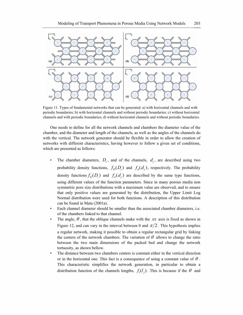
Modeling of Transport Phenomena in Porous Media Using Network Models 203
Figure 11. Types of fundamental networks that can be generated: a) with horizontal channels and with periodic boundaries; b) with horizontal channels and without periodic boundaries; c) without horizontal channels and with periodic boundaries; d) without horizontal channels and without periodic boundaries.
One needs to define for all the network channels and chambers the diameter value of the
chamber, and the diameter and length of the channels, as well as the angles of the channels do with the vertical. The network generator should be flexible in order to allow the creation of networks with different characteristics, having however to follow a given set of conditions, which are presented as follows:
• The chamber diameters, iD , and of the channels, d j , are described using two
probability density functions, fD(Di ) and fd (dj ), respectively. The probability
density functions fD(Di ) and fd (dj ) are described by the same type functions, using different values of the function parameters. Since in many porous media non symmetric pore size distributions with a maximum value are observed, and to ensure that only positive values are generated by the distribution, the Upper Limit Log Normal distribution were used for both functions. A description of this distribution can be found in Mata (2001a).
• Each channel diameter should be smaller than the associated chamber diameters, i.e. of the chambers linked to that channel.
• The angle, θ , that the oblique channels make with the xx axis is fixed as shown in Figure 12, and can vary in the interval between 0 and 2π . This hypothesis implies a regular network, making it possible to obtain a regular rectangular grid by linking the centers of the network chambers. The variation of θ allows to change the ratio between the two main dimensions of the packed bed and change the network tortuosity, as shown bellow.
• The distance between two chambers centers is constant either in the vertical direction or in the horizontal one. This fact is a consequence of using a constant value of θ . This characteristic simplifies the network generation, in particular to obtain a distribution function of the channels lengths, fl(l j) . This is because if the θ and

António A. Martins, Paulo E. Laranjeira, Carlos Henrique Braga et al. 204
the distribution function of the chambers length, fD(Di ), are known, one only needs
to know the distance between one type of chambers centers to determine fl(l j) . In this work it was assumed that the distance between the centers of two chambers linked by an oblique channels is an input to the package.
• The junction of a chamber (sphere) with a channel (cylinder) results in the formation of a spherical cap, as shown in Figure 12. In the calculation of the total volume of network voids the volume of these spherical caps should be taken into account only one time, in order to obtain the total volume of network voids. The thickness , hij , and corresponding void volume of a spherical cap are given by the following expressions
⎥⎥
⎦
⎤
⎢⎢
⎣
⎡
⎟⎟⎠
⎞⎜⎜⎝
⎛−−=
2
i
jiij D
d11
2Dh (41)
⎟⎠
⎞⎜⎝
⎛ += iji
ijCal hD
hV23
π (42)
Figure 12. Scheme of the spherical cap formed in the junction between a chamber and a channel.
Other conditions can be imposed in the model in order to extend its range of applicability,
some of which are described as follows: • As defined above, the coordination number, Ci , represents the number of channels
coupled to a chamber. This parameter value is controlled primarily by the existence or not of horizontal channels and of periodic boundaries. Other form implemented in this work to vary the value of iC and obtain a distribution of values consists in randomly remove channels and/or chambers. In this model its was imposed that the removing process is done to verify an average value of C . The only imposed condition to the model network generator is that each chamber should have at least one entrance channel and one exiting channel, in order to avoid the formation of a line of chambers without channels of entrance and exiting, which would imply a null

Modeling of Transport Phenomena in Porous Media Using Network Models 205
flow through the network. In the network generator it was implemented the options of removing only horizontal channels or removing any type of channel.
• Sometimes one needs to determine the network permeability value, for example for comparison with the experimental value of a porous medium under study. To perform this calculation it is needed to know a thickness value of the network, which is not directly used in the network model, because it is bi-dimensional. The determination of the network thickness was done together with the determination of the channels distribution lengths, imposing two conditions. One condition is the equality between the packed bed porosity and the network porosity. The other condition follows directly from the hypothesis of constant distance between the centers of the chambers.
• One of the conditions already imposed in the model is that of each channel diameter to be smaller than those of the associated chambers. However, if the diameters distribution functions of chambers and channels overlap, the channels may crossover at the chamber effect, and that effect should be taken into account in the volume calculation. Alternatively, it can be imposed the condition that the channels cannot crossover at the chamber entrance. The application of this condition can be very restrictive for situations where there are horizontal channels or where the diameters distribution have very similar average values or when the standard deviation values are large. The application of these conditions for the channels size implies that the network generation is never completely random, making it possible to occur a tendency for the small diameter chambers, when compared to the average value D , to be associated with channels with small diameters. At this stage of development, this situation was not considered in the model.
In another hand, some imposed conditions to the model can be relaxed in a way to
simplify the network generation. • The spherical caps formed by the entrance of the channels in the network chambers
can be neglected, especially when the channels and chambers are not very close to each other.
• Another way to simplify the network creation process is to consider that the chambers and channels diameters have a constant value, similar to having a point distribution. For this distribution, when the boundaries are periodic, the network is named as uniform network, since there are no differences on its local structure.
The last simplification makes it possible, in some limit cases, to analytical model fluid
flow and mass transport in the 2D network, as shown in the next sections.
Geometrical Model
Description As referred before a model that aims to make a satisfactory description of transport
phenomena in a porous media depends largely in its ability of incorporate information about

António A. Martins, Paulo E. Laranjeira, Carlos Henrique Braga et al. 206
its local structure. The failure to do so will limit the validity of the models, that will depend ultimately in parameters fitted to experimental data. Many strategies and experimental techniques were proposed with this intention. The main difficult lies in how the experimental information about the porous media is obtained and it is incorporated in the model.
As stated before, the local structure of a packed bed formed by the deposition of particles in a container can be obtained by a number of methods. Based on that information it is even possible to obtain the equivalent network of simple elements (Thompson and Fogler, 1997; Chan and Ng, 1986 and 1988; Balhoff and Thompson, 2006). These methods do not obtain an exact replica of the local structure, but a analogous structure that, if the real packing was random in size and made of a sufficiently large of particles ensures that behavior predicted by the model is close to the real system. However, this methodology is computationally intensive, and problems may arise when defining the elements of the network and how they are interrelated (Chan and Ng, 1986).
In this article a simple and faster method is presented, developed to be used for packed beds of spherical shaped particles and with a narrow size distribution. The model is based on readily available or easy to determine data, in particular the porosity and particle size distribution.
From all the possible packed beds, those made with particles of the same size with a regular structure are the easiest to characterize. In particular, their behavior can be characterized using a representative cell, reducing enormously the effort needed to characterize them (Hasimoto, 1959; Zick and Homsy, 1982, Sangani and Acrivos, 1982a and 1982b, Edwards et al., 1990). They are six different regular packings, with different geometrical characteristics (Graton and Frasier, 1935; Martin et al., 1951; Pietsch, 1996). In Figure 13 the tri-dimensional structures of each regular packing is presented, and in Table 1 the names of each one as well the corresponding value of porosity are presented (Pietsch, 1996). They encompass a large range of values of porosity, including the values usually encountered in practice, normally around 0.4.
Figure 13. Regular packings of spheres: a) CUB; b) ORT; c)HEX; d) TET; e) RBP; f) RBH.

Modeling of Transport Phenomena in Porous Media Using Network Models 207
Table 1. Porosity values for each of the regular packings (Pietsch, 1996)
Type of Packing Code Porosity Cubic CUB 476 Orthorombic ORT 395 Hexagonal HEX 395 Tetragonal TET 302 Rhomboedral – Pyramidal RBP 260 Rhomboedral – Hexagonal RBH 260
Comparing the porosity values of the various packings, it can be seen that there are two
pairs with the same porosity value: ORT/HEX and RBP/RBH. Their structures are different, implying that their hydrodynamic behavior must be also different. For examples, albeit the packings ORT and HEX have the same structure, depending only in the way they are observed, depending on the main direction of flow the fluid will cross faces defined by four and three spheres in the ORT and HEX packings respectively. Therefore, both structures will have different hydrodynamic behaviors, as shown experimentally by Martin et al. (1951). An analogous situation occurs for the pair RBP/RBH. Both cases are considered explicitly in the development of the geometrical, being the main assumptions listed below.
• As each packing has a regular structure, the values of D , d and l predicted by the
model are spatial independent, vary only from packing to packing, and represent only the average values of the network elements size distributions.
• If the particle size distribution is known, the parameters of the network elements size distribution can be determined directly from it.
• The values of D , d and l calculate for each regular packing are valid only to that value of porosity. If a packing has a different porosity value, it is assumed that the values of D , d and l can be calculated from correlations based on the values determined for the regular packings.
• For the pairs of packings that share the same porosity values it is assumed that D , d and l values are an arithmetic average of the values obtained for the two regular packings.
• As each packing is regular and spatially periodic, the values of D , d and l can be determined directly from the geometrical analysis of the fundamental cells that characterize each regular packing.
The fundamental cells for each packing are presented in Figure 14. Note that each vertex
represents a sphere centre, not represented for sake of simplicity. The details of the geometrical manipulations needed to obtain each representative cell starting from the simplest one (cubic packing) are presented elsewhere (Martins, 2006). Analyzing the different fundamental cells, it is possible to define two different types of faces:
• Square faces, where four spheres touch each other in the same plane, defining the
centers of the spheres a square; • Triangular faces, where three spheres touch each other in the same plane, defining
the centers of the spheres an equilateral triangle.

António A. Martins, Paulo E. Laranjeira, Carlos Henrique Braga et al. 208
Figure 14. Fundamental cells for each of the regular packings.
The total number of faces varies from packing to packing, and the values of each are
presented in Table 2. Note that as the pairs ORT/HEX and RBP/RBH share the same porosity value, they have similar geometrical structures, and shown in Figure 14, and only of them is considered when determining the number of faces in each regular packing. Note that as the pairs of regular packings that have the same porosity have the representative cell (as expected), they have the same total number of faces, square and triangular faces. The different between them will be highlighted below.

Modeling of Transport Phenomena in Porous Media Using Network Models 209
Table 2. Number of faces for each of the regular packed beds of spheres Packing Total Number of Faces Total Number of
Square Faces Total Number of Triangular Faces
Cubic 6 6 - Orthorhombic 5 3 2 Tetragonal 5 2 3 Rhomboedral - Pyramidal 5 1 4 The type and number of faces is used directly in the determination of the values of D , d
and l . Their determination is based on the hypothesis listed below. • The value of D is equal to the diameter of the largest sphere that can be fitted in the
regular packing without changing is structure. • The values of d and l are determined together to ensure that the porosity value of
the representative cell and the regular packing are equal. • The number of channels and chambers associated with a representative cell is equal
to the number of triangular and square faces respectively. The only exception is the CUB packing, where due to geometrical reasons the number of channels is equal to the number of square faces.
• The distance between two contiguous layers of spheres in a regular packed bed and the centre of the two chambers in consecutive lines of the network is equal. In Figure 15 an example can be seen for the CUB packing.
From the previous hypothesis it can be concluded that the value of D can be determined
independently. For the CUB packing the value of D corresponds to the largest sphere that can
be placed inside its representative cell, and equals to ( ) PD13 − . For the remaining regular
packings, D is the largest sphere that can cross a square face, resulting in ( ) PDD 12 −= . Both values are function only of the sphere diameter, and assuming that this relationship is also valid for an irregular packing, D can be expressed in the form ( ) PD DKD ε= , being
DK a function only of porosity. Considering that DK has a polynomial form, and imposing
equal values of DK and a zero value derivative for 3950.=ε , the following interpolation function is obtained
( ) ( ) ( ) 39503950444812 2 ...K D >−+−= εεε (43)
( ) ( ) 395.012 ≤−= εεDK (44)
To be able to obtain the values of d and l the other assumptions are used. First, it is
needed to relate the distance between the centers of two spheres in consecutives lines of the network with porosity. As seen in Figure 15 for a CUB packing, if Fl represents the distance
between the centre of two spheres in contiguous layers and OL the distance between the

António A. Martins, Paulo E. Laranjeira, Carlos Henrique Braga et al. 210
centre of two chambers connected by an oblique channel, both variables are related by the following expression
θcosOF Ll = (45)
Figure 15. Relation of the distance between two contiguous lines of spheres and the centres of two chambers in consecutives lines of the network, for a CUB packing.
The values of l can be calculated from OL using hDLl O 2+−= . The values of Fl
can be determined for each regular packing analyzing how the spheres packed each other. Four different forms of positioning the particles are possible, and for each one Fl is function
only of PD . Also, the geometrical analysis showed that the pairs ORT/HEX and RBP/RBH
have different layer structures, leading to different values of Fl .
Thus, as done for D it can be assumed that ( ) PFF DKl ε= , where ( )εFK is a function only of the porosity. The following third degree polynomial correlates well the values obtained for each regular packing.
( ) ( ) ( ) ( )32 26.057.3726.053.1326.05859.08740.0 −−−+−−= εεεεFK (46)
Note that because it is physically impossible for the regular packings considered in this
work to have layers distanced more than PD , it is imposed that ( ) 1=εFK and the first
derivative of the function ( )εFK is equal to zero for 476.0=ε .
The previous results showed that D and Fl are proportional to PD , being the proportionality constant only function of the porosity. Assuming that this also true for l , and according to the previous equations the following equation follows
( ) ( ) ( ) ( ) ( )εεθεθε hDFl KKsecK,K 2+−= (47)
where hK is obtained from the following expression

Modeling of Transport Phenomena in Porous Media Using Network Models 211
( ) ( ) ( )( ) P
D
dDhPh D
KK
K.K,DKh⎥⎥
⎦
⎤
⎢⎢
⎣
⎡
⎟⎟⎠
⎞⎜⎜⎝
⎛−−==
2
1150εε
ε (48)
The parameter θ can be estimated using the relation between the tortuosity and the
geometrical structure of the network, in particular θ . The relation between θ and T is given by the following relation
θcosLl
LL
TO
F
T
X === (49)
where TL is the total distance traveled by a particle of fluid between the network entrances
and exit, and XL is the network length in the main direction of flow. The tortuosity of a porous medium depends on the porous medium characteristics, in
particular the type of particles and its local structure. Taking into account that the model is based on regular packings of spheres, the correlation of Comiti and Renaud (1989) obtained from experimental data gathered in packings of spheres with a narrow particle size distribution was considered in this work
( )εln.T
49011−= (50)
The value of θ can be expressed as function of T by the formula ( )Tcosar=θ , and,
as T is a function only of the porosity, in this model θ is also only a function of ε . Thus, in the previous expressions all proportional constants will be only functions of the porosity, simplifying the calculations of the average values of the network elements size distributions. Note that if the previous expression for the tuortosity is valid, then the following equation can be written for lK
( ) ( ) ( )[ ] ( )εεεε DFl Kln.KK −−= 4901 (51)
As stated before, the calculation of d and l has to be done simultaneously. According to
the condition imposed above that the porosity or the regular cell is equal to the porosity of the regular packing, and taking into account all previous conclusions, the following system of equations can be written to obtain the values of dK and lK , assuming that they are
proportional to PD and function only of the porosity
( ) ( ) ( ) ( ) ( )θεεθεθε ,2sec, hDFl KKKK +−= (52)
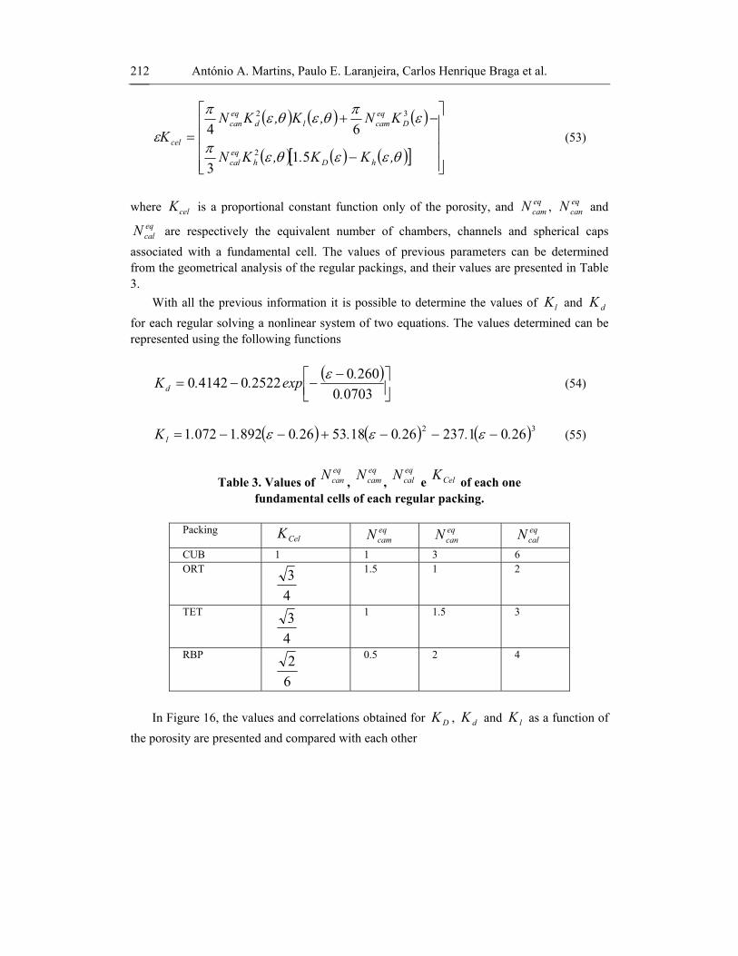
António A. Martins, Paulo E. Laranjeira, Carlos Henrique Braga et al. 212
( ) ( ) ( )
( ) ( ) ( )[ ] ⎥⎥⎥⎥
⎦
⎤
⎢⎢⎢⎢
⎣
⎡
−
−+=
θεεθεπ
επθεθεπ
ε,KK.,KN
KN,K,KNK
hDheqcal
Deqcamld
eqcan
cel
513
642
32
(53)
where celK is a proportional constant function only of the porosity, and eq
camN , eqcanN and
eqcalN are respectively the equivalent number of chambers, channels and spherical caps
associated with a fundamental cell. The values of previous parameters can be determined from the geometrical analysis of the regular packings, and their values are presented in Table 3.
With all the previous information it is possible to determine the values of lK and dK for each regular solving a nonlinear system of two equations. The values determined can be represented using the following functions
( )
⎥⎦⎤
⎢⎣⎡ −−−=
0703026002522041420
..exp..Kd
ε (54)
( ) ( ) ( )32 2601237260185326089210721 .......K l −−−+−−= εεε (55)
Table 3. Values of eqcanN ,
eqcamN ,
eqcalN e CelK of each one
fundamental cells of each regular packing.
Packing CelK eq
camN eqcanN eq
calN
CUB 1 1 3 6 ORT
43
1.5 1 2
TET
43
1 1.5 3
RBP
62
0.5 2 4
In Figure 16, the values and correlations obtained for DK , dK and lK as a function of
the porosity are presented and compared with each other

Modeling of Transport Phenomena in Porous Media Using Network Models 213
Figure 16. Values and correlations obtained or DK , dK and lK as a function of the porosity.
If the distribution of the particle size distributions is known, the geometrical assumes that
the chamber and channel are given by the following expressions
( ) ( ) ( )jP PDDiD DfKDf ε= (56)
( ) ( ) ( )
jP PDdjd DfKdf ε= (57)
They follow directly from the results of the model that showed that for the regular
packings the average chamber and channel sizes are proportional to the average particle size distribution.
Limitations and Comparison with Experimental Data
One of the main limitations of the geometrical model proposed here is linked to the
utilization of regular packings of spheres. Naturally, it is expected that the model will be more adequate for the packings of spheres with a narrow size distribution, homogenous and isotropic. For packing with particles having a shape very different from the spherical or anisotropic, as the model does not include any parameter that takes into account that aspect is not directly applicable in those conditions.
For non spherical particles a possibility of extending the model is the utilization of the concept of sphericity or equivalent particle diameter, based on the ratio between the particles volume and superficial area. However, this strategy is always an approximation and does not take into account the influence the particles in the geometrical characteristics of the void space.

António A. Martins, Paulo E. Laranjeira, Carlos Henrique Braga et al. 214
Also, the particle size distribution should be uni-modal and have a small value of standard deviation. If there are particles of different sizes, or particle size distribution is wide, there is the possibility of obtaining porosity values lower than 0.260 (Yu et al., 1996), and the resulting of channel diameter distribution will have large values of the standard deviation (Nolan and Kavanagh, 1994; Assouline and Rouault, 1996). This is due to the fact the smaller particles can enter in the voids formed by the smaller ones, as shown in Figure 17.
Figure 17. Cut of a packed bed made up of spheres with a wide range of diameters.
Other limitation is the inability of the model to determine the value of C and
corresponding distribution of values, directly from the geometrical analysis of the regular packings. A possible hypothesis was to assume the value of C equal to the number of channels associated with a given fundamental cell. However, due to the geometrical differences between the network model and the packings, it was preferred to maintain C as a free parameter.
Comparison with Experimental Data Even though the experimental data available in literature is dependent on the structure
assumed by the authors for their approximate model of the local structure of the porous media, it is nevertheless instructive to compare the predictions of the model with published data.
Kruyer (1958) has performed porosimetry experiments in packed beds made up of nearly equal sized particles. From the extrusion and retraction curves it is possible to conclude that the pore size distribution, equivalent to the channels in our network model, is very narrow and can be accuretaly described using a single average value. Frevel and Kressley (1963) and Mayer and Stowe (1965 and 1966) confirm these experimental findings, and for a value of porosity around 0.90 they predicted values of dK between 0.27 e 0.37, in agreement with the predictions of the geometrical model.

Modeling of Transport Phenomena in Porous Media Using Network Models 215
Nolan and Kavanagh (1994) simulated the deposition of particles with different particle size distributions and analysed the local structure obtained. Their results showed that the chamber and channel size distributions are a function of the particle size distribution, especially its standard deviation. The predicted values of D by both model agree very well for porosities around 0.40. Chan and Ng (1986 e 1988) also studied packed beds formed by the deposition of nearly equal sized spheres in a rectangular container. For porosities around 0.40, the network model constructed by the authors to represent the packing void space gives values of d and of 0.38 and 0.45, in agreement with the geometrical model. Chu and Ng (1989) used the same strategy, but taking into account the influence of container. In this work the channel length is also evaluated. A value of 251.Kl ≈ was obtained, within the range of values predicted.
The previous results show that the model proposed in this work can predict accurately the average sizes of the network elements that represent the packed beds. For porous media formed by particles with a large range of diameters, the data of Payatakes et al. (1980) shows great differences with the geometrical model, revealing its limitations.
HYDRODYNAMIC MODEL Following the general description of the hierarchical model, the hydrodynamic behavior
in a porous media is based on the modeling of the local structure of a porous medium, made by the network/geometrical model. The main assumptions made during its development and computational implementation are presented bellow.
• The flow is incompressible, monophasic, isothermal and in stationary state. The
transport properties, in particular the flow viscosity and density, are considered constant. The network elements are saturated by the fluid.
• It is assumed that the fluid mixture in the chambers is perfect, which ensures that the pressure on its interior is uniform. The influence of the chambers in the flow is being felt through the links with the network channels and by the mixture of the fluid entering the chamber.
• In the channels there is a plug flow. This hypothesis implies that the velocity profiles in the channels are uniform and uni-dimensional. This way, the pressure drop on a channel can be determined based on a friction factor, function of the flow regimen in the channel.
• The last hypothesis also implies that the effects of the channels entrances and exits on their velocity profiles are negligible. Similarly, the streamlines at the entrance and exit of the channels are parallel among them, simplifying the modeling of the hydrodynamic behavior in the chambers.
The hypothesis imposed in the flow description implies that the velocity and pressures
profiles in the interior of the network are associated to the network channels and branches, respectively. The model implemented to the flow description is described as follows.

António A. Martins, Paulo E. Laranjeira, Carlos Henrique Braga et al. 216
Model Description The modeling of the fluid flow through the network chambers and channels are done by
writing their mass and momentum conservation equations. When describing the balance equations in the channels, the influence of the links among them and the chambers is taken into consideration. The model formulation is based on the analogy between the hydraulic and electric circuits (Dias and Payatakes, 1986a). That is why it is convenient to associate to the circuit nodes and branches the network chambers and channels, respectively.
By applying the analogy with an electric circuit, a system of equations is obtained where the unknowns are absolute pressures in the chambers interior. The nature of the equation system depends on the flow characteristics through the network channels.
The primary variables in the flow description are the volumetric flow rate in each channel, jq , and the absolute pressure in each chamber, iP . The analogous variables are the
electric current intensity in a chamber and the electric potential in each node of the electric circuit respectively. In Figure 18 it is presented an example of an electric circuit equivalent to a chamber with horizontal channels and periodic boundaries. As it was assumed that the flow is on steady state, the analogous application allows one to use the methodologies developed in the analysis of electric circuits (Desoer and Kuhn, 1969).
The mass balance equations on the network nodes can written in the form
∑∑ = Oj
Ej qq (58)
where Ejq and O
jq represent the volumetric flow rate1 in a chamber entrance and exit
channels, respectively. The behavior in the network branches is described by the following equation, similar to the Ohm law that takes into account the possibility of existence of non-linear flow terms.
sjj
sjjjj qRPqRP −Δ+=Δ (59)
The term jPΔ represents the pressure drop in a network branch, equivalent to the
potential difference observed between the nodes and its ends. jR represents the resistance to
the fluid flow through the network branch, including this term the influence of the flow friction in the channel walls and of the connections between chambers and channels. The term
sjPΔ represents tension sources, for example when one considers the influence of the flow
gravity, capillary pressure due to the superficial tension on a multiphase flow (Payatakes and Dias, 1986a), or physical properties variation, as it is the case of the exothermic reactions
occurrence in the medium. The term sjq represents current sources and can be significant in
situation where chemical reactions occur with a variation of the medium moles number.

Modeling of Transport Phenomena in Porous Media Using Network Models 217
Figure 18. Electric analogous used for the flow description: a) electric circuit equivalent to a network with horizontal channels and periodic boundaries; b) analogy for the flow in a channel.
In the hydrodynamic model the flow occurs by imposition of a pressures macroscopic
gradient, imposed between the entrance and exit network channels. This term is considered through the definition of a tension source term associated to the fluid entrance in the network channels. For the remaining channels the following equation is valid
s
jjjj PqRP Δ+=Δ (60)
The mass balance and momentum conservation equations, defined by Equations 58 and
59 respectively, should be solved simultaneously to determine the volumetric flow rates and the absolute pressures in the network channels and chambers respectively. Both types of equations are associated through the term jR that represents the resistance to the flow of a
network branch. The nodes and meshes laws can be applied to the network electric analogous to simplify
the resolution of the equations system and reduce the number of equation to solve simultaneously (Desoer and Kuhn, 1969). The mass balance equations in the chambers, defined by Equation 58, can be expressed in the following matrix form (nodes law)
0=Aq (61)
where q is a vector of CanN elements having the current intensity values on each branch and
A is the matrix of reduced incidences of CanCam NN × dimensions. The elements ija of the
matrix A can take one of three values as a function of the flow direction in the channel j in relation to the chamber i : -1 if the direction corresponds to flow entrance, +1 if the direction corresponds to flow exit, and 0 if the channel and chamber are not liked among them.
Similarly, it is possible to write the meshes law to the electrical analogue. This law says that the different of potential in a closed branch of an electric circuit should equal to zero. The application of this condition results in the following matrix expression
PAP T=Δ (62)
António A. Martins, Paulo E. Laranjeira, Carlos Henrique Braga et al. 218
where PΔ is a vector with CanN elements, containing the differences of potential in each
electric circuit branch, P is a vector with CamN elements, containing the potentials
(pressures) in the circuit nodes, and TA is the transposed incidence matrix. The Equation 61 can be written as follows
( )sjjjj PPGq Δ−Δ= (63)
where
G j =1R j
(64)
jG is the branch conductance. The Equation 63 can be written in the matrix form
( )sPPGq Δ−Δ= (65)
where sPΔ is a vector with CanN elements, containing the tension sources in each network
branch and G is a diagonal matrix of dimensions CanCan NN × , containing the conductance values of each equivalent circuit branch.
Substituting Equation 65 on Equation 62 and rearranging it, an equation system is obtained where the unknowns are the potentials (pressures) in the network nodes, in the form
sqYP = (66)
where the matrix Y is defined by the expression
TAGAY = (67) This matrix Y is the admittances matrix, being a square matrix of dimension
CamCam NN × . The elements ijy can be determined from the matrix G , taking into
consideration their position in relation to the matrix diagonal, in the form: • The elements in the matrix diagonal, iiy , are determined by summing the
conductance of all network branches associated to node i , representing the admittance of a node i .
• The elements that do not belong to the diagonal, ijy , are symmetric to the
conductance value of the branch that links the chambers i and j , representing the mutual admittance between two network nodes.
• All the remaining elements are nulls.

Modeling of Transport Phenomena in Porous Media Using Network Models 219
According to the structure of the network model implemented, the maximum number of channels associated to a chamber is six. This way, each matrix line Y possess in the maximum seven non null values, since the main diagonal is associated to the nodes. This value is function of the coordination numbers distribution of the network chambers, essentially determined by the existence or not of horizontal channels. According to the second rule, as the elements ijy and jiy are equal, Y is a symmetric matrix and positively definite
(Suchomel, 1998a and 1998b). This property of Y is important to the selection of the numerical method used for the solution of the system of equations, in particular when there the number of chambers is large.
The vector sq of dimension CanN represents the influence of the flow and tension sources, and can be determined using the expression (Desoer and Kuhn, 1969)
ss PAGq Δ= (68)
The equation system defined by the previous equation allows the determination of the
potential values in the network nodes, corresponding to the absolute pressures in the chambers interior, know as the conductance matrix, G and the vector sq .
The problem of the flow description through the network chambers and channels is reduced to calculus of the admittance matrix, Y . In the calculus of this matrix one needs to determine the conductance values and of the tension sources associated to each network branch, which is only possible if the geometric characteristics of the network were known, in particular the distributions of the network elements characteristic dimensions.
Modeling of the Network Elements Hydrodynamic In this work it is considered that the network conductance value is the sumo of two terms,
representing the action of the viscous forces on the channels walls and the influence of the expansions and contractions between the chambers and channels, in the form
Ej
Fjj RRR += (69)
where FjR represents the channel resistance due to the friction on the channel wall and E
jR
represents the expansions and contractions resistance of the channels due to the fluid entrance and exit from the chambers. Channels Resistance
For the channels, the flow resistance is due to the flow friction on the channels wall, and
can be written as follows
jF
jF qRP =Δ (70)
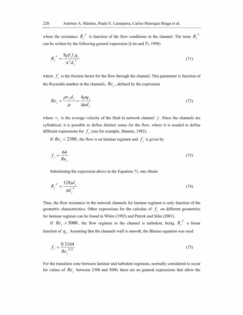
António A. Martins, Paulo E. Laranjeira, Carlos Henrique Braga et al. 220
where the resistance FjR is function of the flow conditions in the channel. The term F
jR
can be written by the following general expression (Lim and Ti, 1998)
52
8
j
jjjFj d
qlfR
πρ
= (71)
where jf is the friction factor for the flow through the channel. This parameter is function of
the Reynolds number in the channels, jRe , defined by the expression
j
jjjj d
qdvRe
πμρ
μρ 4
== (72)
where jv is the average velocity of the fluid in network channel j . Since the channels are
cylindrical, it is possible to define distinct zones for the flow, where it is needed to define different expressions for jf (see for example, Shames, 1982).
If 2300<jRe , the flow is on laminar regimen and jf is given by
jj Re
f 64= (73)
Substituting the expression above in the Equation 71, one obtain
4
128
j
jFj d
lR
πμ
= (74)
Thus, the flow resistance in the network channels for laminar regimen is only function of the geometric characteristics. Other expressions for the calculus of jf on different geometries
for laminar regimen can be found in White (1992) and Patzek and Silin (2001).
If 5000>jRe , the flow regimen in the channel is turbulent, being FjR a linear
function of jq . Assuming that the channels wall is smooth, the Blasius equation was used
250
31640.
jj Re
.f = (75)
For the transition zone between laminar and turbulent regimens, normally considered to occur for values of jRe between 2300 and 5000, there are no general expressions that allow the

Modeling of Transport Phenomena in Porous Media Using Network Models 221
calculation of jf , due to the large dispersion of available experimental values (Shames,
1982). However, to model the flow in a network of chambers and channels when the value of
jRe fall within that range, there is the need for a continuous expression of jf as a function
of jRe . Two strategies were considered. In the first one, jf is approximated by linear
interpolation between the friction factor values for the superior and inferior extremities of the laminar flow zones, Re j = 2300 and turbulent, Re j = 5000, respectively.
This approximation assures the continuity of jf in the extremes of the transition zone,
but not of first derivative of the function jf . Depending on the algorithm used for the
equation system resolution, the existence of this type of discontinuities may bring numerical problems, especially when there are many network channels where the flow conditions are close to the limits between the two flow regimens (Bending and Hutchison, 1973).
Another way to determine jf was developed in order to guarantee the function
continuity and of the first derivative in the limits of the transition zone, using Tchebyshev polynomials (Conte and De Boor, 1984). In this case the limit values of jRe were
simultaneously determined with the polynomials coefficients. Both approximations are compared in Figure 19. It is observed that both curves are
similar, occurring the larger differences in the limits of the definition of the linear fitting. The transition zone defined by the Tchebyshev polynomials is larger than the linear approximation, reducing especially the laminar regimen zone.
Figure 19. Comparison of the jf curves as a function of jRe in the transition zone for both forms of
fitting proposed. The hydrodynamic simulator allows the utilization of any approximation, being preferred
the second one as the function ( )jj Ref is continuous and has continuous first derivatives in

António A. Martins, Paulo E. Laranjeira, Carlos Henrique Braga et al. 222
all the values range of Reynolds numbers. However, the linear approximation simplifies the analytical description of the flow, as one it will be further described in this paper.
Chambers Resistance
For the chambers, the resistance to the flow, EjR , is associated to connections between
chambers and channels. For practical questions, this term is associated to the network branches, as shown to Figure 20. Since normally there are two chambers associated to a
branch, one needs to sum the contributions from each side to determine EjR .
Figure 20. Schematic representation of the resistance of the branch and electric analog utilized.
The value of EjR is the sum of two contributions
ET
jEL
jE
j RRR += (76)
The first term, ELjR , represents the contribution of the viscous strengths and the second
term, ETjR , represents the contribution of the inertial effects.
For the first term, the results Koplik (1982) were used. This author solved analytically the creeping flow problem for a chamber/channel geometry similar to the one used in this work,
demonstrating that ELjR can be calculated with a small error assuming that the channel j
has an additional length extension in the chamber interior equal to πjd2 . Substituting in
Equation 74, and taking into consideration that each branch has two chambers on its
extremes, ELjR can be expressed in the form
32
512
j
ELj d
Rπ
μ= (77)
The second term, ETjR , represents the inertial effects contribution and their value can be
determined analyzing the chamber flow, in particular in the connections between the chambers and channels. Theoretically it is possible to describe the flow solving the mass and momentum conservation equations written for the network chambers and channels. In this

Modeling of Transport Phenomena in Porous Media Using Network Models 223
work a simpler strategy is considered, based on the calculation procedure normally used to determine the pressure drop due to accidents in pipes and flow systems (Shames, 1982; White, 1992), the jK method.
In the ETjR determination one needs to take into consideration that there are two
accidents associated to each network branch with distinct hydrodynamic behaviors. Despite the fact that jK is a function of the network flow and geometric characteristics at local level,
it is assumed a constant value for the expansions and contractions. This way, ETjR is
calculated using the following expression
∑∑==
==2
142
2
142
88k
jj
j
k
kj
j
jETj K
d
qK
d
qR
π
ρ
π
ρ (78)
where the parameters kjK account for the influence of the flow expansions and contractions.
Although there are in literature expressions that allows one to estimate kjK as a function of
the network elements diameters associated among them, these are only valid for cases involving only a chamber and a channel. Thus, these expressions are not applicable to the network structure considered in this work, and ∑ jK is then determined by fitting the
predicted values by the hydrodynamic simulation with experimental data obtained in literature, making it possible to directly include in the flow simulation the network structure. Network Branch Resistance
The total resistance of a network branch, jR , is obtained by summing the different terms
of flow resistance, obtaining the following general expression as a function of the channel diameter.
423252
85128
j
jj
jj
jjjETj
ELj
Fjj d
Kqdd
lqfRRRR
πρ
πμ
πρ ∑++=++= (79)
where jK∑ is the sum of the constant jK associated to a certain network branch. The first
term represents the influence of the flow in the channels and the last two terms the influence of the connections between chambers and channels, composed by two terms in order to distinguish the influence of the viscous and inertial forces. For laminar flow in the channels the previous equation can be expressed in the form
( ) 4242
84128
j
jjjj
j
ETj
ELj
Fjj d
Kqdl
dRRRR
πρ
ππ
μ ∑++=++= (80)

António A. Martins, Paulo E. Laranjeira, Carlos Henrique Braga et al. 224
Assuming that the chambers influence on the flow is negligible, only taking into consideration the friction influence of the flow in the channels wall, the previous expression can be simplified to the following expression
4
128
j
jFjj d
lRR
π
μ== (81)
that is equivalent to the Poiseuille equation for the flow in circular tubes. The model predictions with or without the resistance terms associated to the chambers will be further compared, in order to identify the relevant flow effects. System Solution
The resolution of the equation system defined in the matricial form by the Equation 66 allows one to obtain the pressure values at the network nodes. The most adequate strategy to solve the equation system depends essentially on the nature of the system and on the model selected for the calculus of jR , in particular when the flow conditions are non linear. In order
to obtain the solution more efficiently, it is important to take into consideration their properties. Independently of the conditions imposed to the network generator and to the hydrodynamic simulator, the equation system is symmetric and sparse. Each line of the coefficient matrix Y possesses in the maximum seven non zero elements, this situation occurring for a network with horizontal channels and periodic boundaries.
Since the characteristic dimensions of the network elements are described by probability density functions, the results obtained by the hydrodynamic simulator are statistically valid if the networks have a large number of elements. As for the networks with a large number of elements almost all the Y elements are zero, the algorithm being implemented should take into consideration this aspect, in order to avoid doing an excessive number of meaningless (Pruess et al., 1992).
The nature of the system of equation system being solved depends on the selected model to the calculus of jR and on the conditions imposed to the hydrodynamic simulator, in
particular the limit conditions between the several flow regimens. If the jR values are
independent from jq , characteristic of the laminar flow regimen, the system of equations is
linear. Suchomel et al. (1998a) showed that the system coefficient matrix, behind being symmetric and sparse, also it is positively defined, which makes it possible to use efficient interactive methods for the resolution of the linear equation system. In this case it was used the DSRIS routine from the scientific library ESSL (IBM), that uses the generalized steeptest descent method that takes into consideration the symmetric nature of the coefficient matrix. In the case the inertial terms are significant, the equation system is non linear, being solved
using a fixed point method. Since the non-linear resistance terms, ETjR , are a function of
jq , it is need to define an initial estimation of the flow rates values in the network channels.
Since it is possible in practice to know if the equation system is linear or non-linear from the imposed value of TPΔ , of the network geometric characteristics and of the selected model for

Modeling of Transport Phenomena in Porous Media Using Network Models 225
the jR calculus, the algorithm assumes for the first iteration that the flow is in laminar
regimen in all the network elements. This way the ETjR values are equal to zero and the
equation system is linear, making it possible to use the usual methods to solve it. The algorithm stops if the flow is laminar in all the network channels, or when the following convergent criterion is verified
( )( ) tolN
j
kj
N
j
kj
kj
Can
Can
q
qqε<
−
∑
∑
=
=
−
1
2
1
21
(82)
where k refers to the iteration number and tolε is the maximum tolerance imposed to the iterative process, being this value imposed by the user. A similar algorithm was used by Sorbie et al. (1989) for modeling non-Newtonians fluid flow modeling in purely viscous regimen through the porous media, using a bi-dimensional network only composed by channels. In this problem, the non-linear terms also occur in laminar regimen, since the fluid viscosity is a function of the flow characteristics in the channels. As an initial estimative, Sorbie et al. (1989) used the flow profile for Newtonian fluids in laminar regimen, correcting successively the viscosity values according to the flow characteristics in the channels. The performance of the proposed algorithm was satisfactory in all the cases analyzed by these authors.
Sahimi (1993) and Wang et al. (1999a) also analyzed the flow of non linear fluid through a porous medium utilizing network models, and solved the non-linear equation system by the Newton-Raphson method. Shah and Yortsos (1995) used the successive over-relaxation, to the flow modeling of non-Newtonian fluids through a porous medium. This methods does not need to have a good estimation as the Newton-Raphson method requires and it is more robust.
Special Case of a Regular Network
A regular network is a network that possess the following characteristics: • the chamber and channeld diameter, and the channel length, take only one value; • the coordination number is equal for all network, implying that the boundaries have
to be periodic. In a network with those properties, it can be shown that the hydrodynamic behavior can
be characterized analytically (Martins, 2006). The relation between the total pressure, TPΔ ,
and flow rate, Tq , through the network can be expressed in the form
( ) ( )y
Tjxjx
N
jjT N
qRNpNpP
x
211
1
1+=Δ+=Δ=Δ ∑
+
= (83)

António A. Martins, Paulo E. Laranjeira, Carlos Henrique Braga et al. 226
Using the expressions proposed before for jR , its is possible to determine either TPΔ or
Tq , depending if Tq or TPΔ are known. A list of expressions that can be used to determine
either TPΔ or Tq can be found in Martins (2006). From those expressions analytical expressions for k and the constants A e B of the MacDonald equation can be also easily obtained. Details of their determination and their analysis are given in Martins (2006).
For example, the expressions for the network permeability not considering the volume of spherical caps and assuming that the network is large are the following
( )[ ]
( ) ( ) ( )dlDldD
dDlk41sin21sin2
32
cos16
2
3
22
+⎥⎦
⎤⎢⎣
⎡−+++
+≈
πθθ
εθπ, 6=C (84)
( )[ ]
( )dlldD
dDlk4
31
cos32
2
3
22
+⎟⎟⎠
⎞⎜⎜⎝
⎛+
+≈
π
εθπ, 4=C (85)
From the previous expressions it can be concluded that the permeability depends not only
on the characteristic dimensions of the network elements, but also on the geometrical structure through θ . The permeability has the expected dependency on the value of d (Dullien, 1992; Guyon, 2005), but, keeping d constant and varying D a distinct behavior can be observed.
Considering the geometrical model and assuming 4=C , the permeability of a packed bed as a function of the permeability is given by the expression
( )[ ]
( )
2
2
3
22
431
cos32 P
Dlld
D
dDl DKKK
KK
KKKk
+⎟⎟⎠
⎞⎜⎜⎝
⎛+
+≈
π
εθπ (86)
The previous expression predicts that permeability is a function of 2PD , as expected
(Dullien, 1992). For a uniform network with 6=C similar expressions are obtained, and the same dependence of k is observed.
Data Treatment The main results of the network are the pressure and flow field. The values of the
permeability can be obtained using the following expression

Modeling of Transport Phenomena in Porous Media Using Network Models 227
TRY
XT
TN
XT
PELLq
PALqk
Δ=
Δ=
μμ (87)
where Tq is the total flow through the network, calculated summing the flow rates in the channels exiting the network. Note that in the previous equation a value of the equivalent thickness is defined, resulting from the fact the permeability is defined as a function of the superficial velocity in the network. The constants A e B can be determined using the representation of the in terms of *F vs *Re , and knowing that the MacDonald equation can be represented in the form (see part A for more information)
BReAF += *
* (88)
When the flow is linear, corresponding to low values of *Re , the value of A is given by the
ordinate in the origin of the curve of *F as a function of *Re , a linear relation in logarithmic coordinates with a slope equal to -1. The value of the constant B is determined in non linear flow regimen, for high values of *Re , where the curve *F as a function of *Re tends a constant value equal to B . Sensitivity Analysis
Analysis of the Resistance Terms Relative Importance
One of the key aspects of fluid model proposed in this work is the explicit calculation of the resistance terms associated with the interconnections between the chambers and channels. Although physically more detailed, it is not clear which terms are relevant for which flow regimen. Thus, in Figure 21 the curves of *F as a function of *Re are given with
connections and without connections, where 0=∑ jK , thus 0=ETjR , and 0=EL
jR .
Also, the MacDonald equation is represented in the figure to determine, from a qualitatively pointo of view, which model better describes qualitatively the behavior observed in practice. The results show that for low values of *Re , corresponding to linear regimen and dominance of the viscous forces, similar behavior is observed with or without entrance effects. As the value of ET
jR is small when compared with other remaining terms, and ELjR and F
jR predict
similar behavior for this range of *Re values. The differences observed between the curves are due to the inclusion or no of EL
jR , a term small when compared with FjR .
For high values of *Re large differences can be observed between the predictions made with or without the entrance effects. In particular, the transition is smooth and starts in the range of modified Reynolds numbers between 10 and 100. The results are also on qualitatively agreement with the MacDonald Equation. When the entrance effects are not considered, the transition occurs for much higher Reynolds numbers and do not show the

António A. Martins, Paulo E. Laranjeira, Carlos Henrique Braga et al. 228
smooth behavior of the MacDonald equation. Thus, it can be concluded here that only when all the resistance terms are considered is the model able to describe all the regimens observed for flow in a packed bed, in particular the transition zone.
Figure 21. Plot of *F as a function of *Re , with and without the entrance effects between chambers and channels.
Network Size Effects
The network elements characteristic sizes follow given statistical distributions. Thus, it is necessary to determine how large the network have to be to ensure that the results are statistical significant. From a practical point of view, the larger the network the smaller the variance associated with the predicted values, since the larger the samples obtained from the distributions the better.
In Figure 22 the values of permeability are presented as a function of yN , for three
values of xN . Networks with horizontal channels and periodic boundaries, 50.Dd = with
0040.D = and 00700 .l = fixed (all size dimensions are in meters), and 4πθ = were
considered. Two sets of values of standard deviation are considered: 050.dD == σσ and
400.dD == σσ . For each set of values of xN and yN twelve simulations were
performed varying the seed of the random number generator. In both cases it is observed that if 100≥xN and 100≥yN the values of permeability tend to a limit value. Although the
error bars are larger when the values of the standard deviation are high, in both cases they diminish with increasing values of xN and yN . Thus, for networks that verifies the criteria
given above it can be assumed that the results obtained are statistical significant.

Modeling of Transport Phenomena in Porous Media Using Network Models 229
Figure 22. Permeability and a function of yN for three values of xN and two set of values of Dσ
and dσ : a) 050.dD == σσ ; and b) 050.dD == σσ .
Identical behavior was observed independently of the value of C , type of boundary and
flow regimen, thus showing that the main factor controlling the statistical significance of the results is the total number of elements in the network. For the remainder of this article, all results dealing with the flow modeling considered 100×100 networks (first the value of xN
followed by yN ), 50.Dd = with 004.0=D and 0070.l = . If different values are used
in the text they are explicitly stated in the text.
Influence of the Network Characteristics Of the various network parameters and conditions that can be imposed, a qualitatively
analysis reach the conclusion that the main factors controlling the network behavior is the distribution of coordination number, iC . The remaining factors, type of boundaries and value
of θ are not significant. For statistical significant networks, varying the type of networks

António A. Martins, Paulo E. Laranjeira, Carlos Henrique Braga et al. 230
does not change appreciably the total number of elements, the key factor behind the network behavior, thus not changing significantly the predictions of the model. For the second factor, neither term of resistance is function of θ , thus, no change in the flow behavior is observed.
Two forms of varying the coordination number were considered: by the inclusion or no horizontal, or by randomly removing channels. In this last form, two variants were considered: removing only horizontal channels or removing horizontal and oblique channels regardless or their characteristics. Both processes have different impacts when analyzing the local structure that results from the removal process. In particular, removing only horizontal channels maintains the structure of the oblique channels, the elements controlling the flow field, situation not observed in the other form of removal.
To better assess the relative impact of both forms, the best way is to compare the values of permeability predicted by the model for networks with the same value of C but obtained using the two forms. To show the different effects of the removal process, the values of the ratio 6kkC as a function of C are presented in Figure 23, for 40.0== dD σσ . In any
case, a network with 6=C and periodic network boundaries was the starting point for the removal process. The comparison between the results shows that the removal process have a profound impact in the behavior predicted by the model. In particular, removing only horizontal channels leads to an increasing in k , whereas the removal of any kind of channel reduces k .
When any kind of channel can be removed, including oblique channels, the number of paths available to the fluid will be reduced. Hence, the global flow resistance will increase, leading to lower values of the permeability. When only horizontal channels are removed, the structure of the oblique channels is maintained. Thus, the main effect controlling the permeability value is the variation of void volume, necessary to calculate the value of the equivalent network thickness.
For a uniform network the flow rate in the channels is null, and it can be shown that the ratio 6kkC can be expressed in the form (see Martins, 2006, for more details)
223
2236
6 22
362
362
dlCldD
dlldDVV
kk
h
hC
V
VC
⎟⎠⎞
⎜⎝⎛ −++
++≈= (89)
where hl is length of a horizontal channel in a uniform network. The previous expression
predicts that there is a linear relation between k and C in a uniform network, in agreement with the results presented in Figure 23.

Modeling of Transport Phenomena in Porous Media Using Network Models 231
Figure 23. Permeability ratio for the cases of removal of channels or only horizontal channels.
Influence of the Elements Characteristics
The network elements are characterized by their characteristic size distribution. Since the resistance to the flow is a function of the channel diameter, it can be predict that it will be that parameter that will have a more profound impact on the hydrodynamic model predictions.
To show that this is correct in Figure 24 the values of permeability are presented as a function of the ratio Dd for the cases where D or d is kept constant. Note that due to the restrictions imposed in the network generator, this ratio an vary only from 0 to 1. Two sets of values of standard deviation are considered: 050.dD == σσ and 400.dD == σσ . The values obtained assuming that the network is uniform are also present, to assess if that approximation is a valid one.
The results show good agreement between the permeability values obtained for the uniform network and using low values of the standard deviation. Thus, it can be concluded that the results are adequate for network with narrow distributions of the network elements characteristic dimensions. For larger distributions, the deviations increase the larger the value of d is. This is a direct result of the restrictions imposed between the values of D and d at the local level, that when Dd ≈ will lead to a move of the distribution of values of d to lower values, resulting in a higher resistance to the flow than expected.
In Figure 25 the values of permeability as a function of d are presented for 250.Dd = or D constant and equal to 0.004. Networks with the same geometrical
characteristics as those used in the previous figures were also considered here. The predictions of the uniform network are also presented, confirming the results the preceding conclusions that this model is valid if the values of Dσ and dσ are small.

António A. Martins, Paulo E. Laranjeira, Carlos Henrique Braga et al. 232
0.001
0.01
0.1
1
10
0 0.2 0.4 0.6 0.8 1
σ d = σ D = 0.05
σ d = σ D = 0.40
k ttanconsd
ttanconsD
Dd
Uniform
Figure 24. Permeability values as a function of Dd keeping D or d constant.
When Dd is kept constant, the permeability is a function of 2d for all range of values.
However, when D is constant, it is possible to observe two different zones. For low values of d , the permeability is proportional to 3d , difference from the dependence on 2d observed for high values of d .
0.001
0.01
0.1
1
10
0.0001 0.001 0.01
σ d = σ D = 0.05
σ d = σ D = 0.40k
ttanconsD
Uniform
d
250.Dd =
Figure 25. Permeability values as a function of d for 250.Dd = or D constant.
Comparison with Experimental Data The validity of the flow model is ultimately assessed comparing its predictions against
experimental data. Because the geometrical model will be used simultaneously, the main restrictions of that model have to be considered. Thus only data obtained for packed beds made up by nearly sized spheres should be used.

Modeling of Transport Phenomena in Porous Media Using Network Models 233
The experimental data of Kim (1985) was selected because it verifys the conditions of applicability of the geometrical and includes the linear and non linear regimens of flow. In Figure 26 the predictions of the hydrodynamic model are compared with experimental data, varying C and ∑ jK . The results show that only when 4=C is the model capable of
describing the behavior of a real packed bed. This fact aggress with the experimental results of Sederman et al (1997, 1998) and Baldwin et al. (1996), that obtained experimentally using NMR values of C between 4 and 5. Using other experimental techniques, Yanuka et al. (1986) obtained similar values. For 4=C , the agreement is good for all values of ∑ jK
considered, being better when 3≈∑ jK . For the data presented, the best fitting occurs for
48.3=∑ jK .
1
10
100
1 10 100 1000
2.1,6 == ∑ jKC
2KIM
4=C4=∑ jK3=∑ jK2=∑ jK
*Re
*F
Figure 26. Comparison between the predictions of the hydrodynamic model and the experimental data of Kim (1985), as a function of C and ∑ jK .
In Martins (2006) more comparisons between experimental data and the predictions of
the model can be found, all confirming the previous conclusions.
MASS TRANSPORT According to the model proposed in this work, the transport of mass in the network is
based on the description of the local structure, performed by the network of elements coupled with the geometrical model, and of flow field inside the network. Although in some situations the determination of the flow field and the dispersion of mass are linked together, as for example when a perturbation with a high concentration of solute is imposed at the fluid entrance or a exothermic reaction occurs in the media, here its is assumed that the flow and

António A. Martins, Paulo E. Laranjeira, Carlos Henrique Braga et al. 234
the transport of mass do not interfere with each other, allowing the decoupling the system of balance equations. This condition is valid in the tracer limit, where the solute concentrations are low everywhere in the porous medium and do not change appreciably the physical properties of the fluid, or when the solutes particles are indistinguishable from the fluid particles.
In the next sub-sections it will described and analyzed in detail how the mass transport in the network elements can be modeled, the algorithm implemented to solve the mass balance equations, and how the network geometrical and flow field characteristics influence the dispersion of mass. At this stage only a qualitatively analysis will be performed. In future publication the predictions of the model will be compared with experimental data.
Model Description As stated before, the transport of mass inside the network elements will rely on the results
obtained by the network/geometrical and flow models describe above in this article. Following the main assumption of this model, the simulation of the dispersion of mass can be done independently, though it must be done after the determination of the flow field. In brief, the model that will be described aims to determine the behavior of the network model, and consequently of a porous medium, from the response obtained to a perturbation in the concentration fed to the network.
General Model
Using the hypothesis made before in the flow modeling, it can be concluded that the chambers behave as perfectly mixers and the channels as plug flow units. Thus, the channels will be responsible for the mixing of the solute, corresponding to dispersion, and the channels will be responsible for the transport of mass, corresponding to convection. So, different mechanisms of mass are responsible by different mass transport mechanisms.
Base on the behavior imposed for the network elements, and assuming no chemical reaction or interfacial mass transfer, the dimensionless mass balance equations for the chamber i and channel j can be written in the form
( ) ( ) ( )∑=+
jj
Eiji
ii tftf
dttdf
,1ατ (90)
( ) ( )
0,,
=∂
∂+
∂
∂
ztzf
ttzf jj
jτ (91)
where t represents time; z is the axial coordinate in the channels normalized by the channel length jl ; if and jf are the dimensionless concentrations inside the channels and chambers
respectively; Eijα is the total fraction of flow that enters chamber i through channel j , and

Modeling of Transport Phenomena in Porous Media Using Network Models 235
iτ and jτ are the passage times through the chambers and channels, respectively. The
dimensionless concentrations and parameters are defined by the following expressions
( ) ( )( ) ><
=t,yC
tCtf i
i0
( ) ( )( ) ><
=t,yCt,zC
tf jj
0
(92)
( ) ( )( ) ><
=tyCtyCtyf
,,,
0
00
∑=
s
ii q
Vτ ,
j
jj v
l=τ
∑=
s
EjE
ij qq
α (93)
where ∑ sq is the sum of the flow rates exiting the chamber, determined from the global
mass balance; iV is the volume of the chambers; jv is the fluid velocity inside the channels; E
jq is the flow rate in the chamber i and channel j ; and ( ) >< t,yC0 is a reference
concentration that renders the chambers and channels concentrations dimensionless. The correct value of ( ) >< t,yC0 depends on the characteristics of the perturbation imposed. In some cases its value its value is self evident, as for example in a spatial uniform step, where
( ) >< t,yC0 = 0C , being 0C the concentration limit value. In other cases, ( ) >< t,yC0 may be equal to an average of the solute concentration entering the network, although the correct definition may vary depending on the situation.
Considering the overall mass balance written for a chamber it can be shown that
1=∑ Eijα . The distribution of values of E
ijα is a measure of the influence of the local
flow field in the dispersion of mass. The wider the distribution the more important the dispersion of mass will be.
The following set of initial and boundary conditions must be used to solve the system of mass balance equations
( ) ( ) 0000 ==⇒>= t,zf,tfz,t ji (94)
( ) ( )t,yft,ft Ej 000 =⇒> (95)
where y is the spatial direction normal to the main direction of the flow. The first equation implies that when the concentration perturbation is applied the network has no solute. The second condition is the definition of the dimensionless concentration perturbation that it is imposed at the network entrance. The function ( )t,yf 0 can be a function of time, space, or both, and can be defined in many different forms, ranging from the simple, such as step or pulse uniform perturbations, or more complex such as spatially non uniform or random perturbations.

António A. Martins, Paulo E. Laranjeira, Carlos Henrique Braga et al. 236
Algorithm Implemented to Solve the System of Mass Balance Equations The solution of the general system of equations can only be accomplished if their
mathematical properties are accounted for explicitly, both when solving them as well in the definition of the convergence criteria.
A key aspect that has to be considered when solving the system of differential equations is the need to keep the concentration for previous times. From a practical point of view, the concentration that enters a given chamber at time t through channel j is the concentration that was observed in the chamber or outside the network, depending on the relative position of the chamber on the network, but for a time jt τ− . In other words, the channels act as pure
delays, and incorporating it on the mass transport equations the following general expression is obtained
( ) ( ) ( )∑ −=+
jjij
Eiji
ii tftf
dttdf
τατ (96)
where ( )jij tf τ− represent the concentration in the chamber i on the inlet of channel j for
a time jt τ− .
The system of equations now corresponds to a system of delay differential equations, where the solution depends on the all solution history and not only on the initial and boundary conditions. (Haier et al., 1987). They arise and are important to describe the behavior of systems and processes which behavior depends on their evolution in time. Examples include the study of population dynamics (Bocahrov and Rihan, 2000), epidemiology (Nelson and Pereelson, 2002), control systems (Ramirez and Puebla, 1999), among others. Reviews of applications and numerical methods available to solve this type of differential equations can be found in the works of Baker and co-workers (1994 and 1995).
The solution of the system of modified mass balance equations was done using a Runge-Kutta method of fourth order. Some key aspects have to be taken into account when solving it. First a time increment tΔ must be defined. Because our goal is to describe as accurate as possible the behavior of all network elements, tΔ is defined as a percentage of the minimum values of the passage time distributions of both channels and chambers. These distributions can be obtained directly from the geometrical and flow field characteristics of the network. This procedure ensures that the behavior of all the network elements is properly considered.
Second, when solving the mass balance equation for chamber i , it is necessary to know how ( )tf i changes in time. From the general mass balance, Equation 96, it is clear that it is
only need to know the history in the interval [ ]maxjt,t τ− , where max
jτ represents the
maximum value of the flow time passage in the channels j that enter the chamber i .
In practice this is done dividing the channels in INCjN points, where
( )tIntN jINCj Δ= τ . In each time step, the values of ( )tf i are calculated first, based on the
values of ( )ttf i Δ− . After, the values of ( )t,zf j are updated, starting from the entrance to
the exit of the fluid in the channel j . This updating process is analogous to the traveling of

Modeling of Transport Phenomena in Porous Media Using Network Models 237
the concentration wave between two spatial positions inside the channels, and is akin to a particle tracking method, here applied instead to the concentration of solute. Thus the classification of this methodology as a mix between particle tracking and mass balance models. Instead of following the evolution of a cloud of particles, one follows the spatial and time evolution of the local concentration field, after imposing a concentration perturbation at the fluid entrance.
Other key aspect is the convergence criteria. In contrast with the flow modeling, here it is not possible to define unambiguous stop criteria. In this work a combination of criteria was considered, depending the possible combinations on the characteristics of the perturbation imposed at the network entrance. Whenever one of the criteria is met, the simulation stops.
The general stop criteria, independent of the perturbation properties, is to define a maximum simulation time, proportional to the network passage time, Gτ . This ensures that the simulations came to an end, although an adequate time depends on the geometrical and flow characteristics of the network. For perturbations that tend to a constant value for long times ( )Gt τ>> , such as uniform step, the simulation stops if the overall mass balance is verified within a small error. In this work this criterion was implemented only for the uniform step and pulse perturbations. Also for those types of perturbations, a third stop criteria was defined based in the expected limit criteria. For example, for a uniform step it is expected that the limit exit concentration will approach the step concentration. When the entrance and exit by a sufficiently small amount, it can be considered that the simulation reached the steady state and can be stopped. For all simulations performed a combination of criteria was always used.
Strategies to Reduce the Effort Needed to Simulate Mass Transport
The general algorithm presented in the previous sub-section is capable of describing the transport of mass inside a network of elements regardless its geometrical characteristics. However, in some situations the effort needed to solve the equations and obtaining the concentration profile can be prohibitive, thus the interest in developing strategies to reduce the overall effort. Three forms were considered in this work.
The first considers network with horizontal channels or wide distributions of the network elements size. In these networks, the velocity of the fluid in the channels will also have a wide distribution, situation that will lead to prohibitively small values of tΔ . Noting that
channels with low values of jv correspond low values of Eijα , from Equation 96 it can be
concluded that the influence is significant only if Gt τ>> . Also, as it was concluded in the
flow modeling that the best agreement was obtained for 4=C (networks without normal channels), a similar situation was considered to be valid for the modeling of the mass transport in the network. Therefore, only network without horizontal channels were considered in this work.
The second strategy can be applied for perturbations that tend to a constant value for long times, and only to the chambers. It stems directly from the characteristics of those kind og perturbations, where ( )tfi will always tend to the limit concentration defined by the perturbation given enough time. When this situation is reached, solving the mass balance
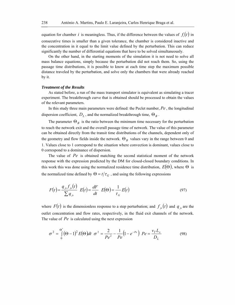
António A. Martins, Paulo E. Laranjeira, Carlos Henrique Braga et al. 238
equation for chamber i is meaningless. Thus, if the difference between the values of ( )tfi in consecutive times is smaller than a given tolerance, the chamber is considered inactive and the concentration in it equal to the limit value defined by the perturbation. This can reduce significantly the number of differential equations that have to be solved simultaneously.
On the other hand, in the starting moments of the simulation it is not need to solve all mass balance equations, simply because the perturbation did not reach them. So, using the passage time distributions, it is possible to know at each time step the maximum possible distance traveled by the perturbation, and solve only the chambers that were already reached by it.
Treatment of the Results
As stated before, a run of the mass transport simulator is equivalent as simulating a tracer experiment. The breakthrough curve that is obtained should be processed to obtain the values of the relevant parameters.
In this study three main parameters were defined: the Peclet number, Pe , the longitudinal dispersion coefficient, LD , and the normalized breakthrough time, BΘ .
The parameter BΘ is the ratio between the minimum time necessary for the perturbation to reach the network exit and the overall passage time of network. The value of this parameter can be obtained directly from the transit time distributions of the channels, dependent only of the geometry and flow fields inside the network. BΘ values vary in the range between 0 and 1. Values close to 1 correspond to the situation where convection is dominant, values close to 0 correspond to a dominance of dispersion.
The value of Pe is obtained matching the second statistical moment of the network response with the expression predicted by the DM for closed-closed boundary conditions. In this work this was done using the normalized residence time distribution, ( )ΘE , where Θ is
the normalized time defined by Gt τ=Θ , and using the following expressions
( ) ( )∑
=js
jsjs
qtfq
tF ( )dtdFtE = ( ) ( )tEE
Gτ1
=Θ (97)
where ( )tF is the dimensionless response to a step perturbation; and ( )tf js and jsq are the
outlet concentration and flow rates, respectively, in the fluid exit channels of the network. The value of Pe is calculated using the next expression
( ) ( )∫ Θ−Θ=Θ*
0
22 1 dtEσ ( )PeePePe
−−−= 1122
2σ L
xT
DLv
Pe = (98)

Modeling of Transport Phenomena in Porous Media Using Network Models 239
Special Case of a Regular Network In the flow modeling it was shown that a regular network is a special case where an
analytical solution of the flow field is possible. The same situation occurs in the modeling of mass transport.
For a uniform network, the flow rate in the normal channels is equal to zero and equal for all oblique channels. Thus, the time to reach a chamber in a line of the network is independent of the particle path through the network, and depends only in the conditions imposed the network entrance. Thus, to be able to obtain an analytical solution it must be also imposed that the concentration imposed has to be spatially uniform.
If those conditions are met, the response of the network model and a model composed by channels and chambers in series is equivalent. To the analogy be correct it is necessary to define a correct passage time for the chambers, *
iτ , that takes into account that in the network
two channels goes to a given chamber, in the analogue only one. Thus, *iτ is defined by the
expression
j
i*i q
V2
=τ (99)
where iV is the volume of the chamber and jq is the flow rate in the channels of the uniform
network. Assuming that there is no chemical reaction and mass transfer between phases, the
system is linear and the ( )sG can be expressed in the form
( ) ( )[ ]sNexps
sG jx
N
i
x
ττ
11
1* +−⎟⎟
⎠
⎞⎜⎜⎝
⎛+
= (100)
The residence time distribution ( )tE is obtained inverting ( )sG . Using the previous
equation the expression for ( )ΘE can be written in the form
E Θ( )=0 Θ < ΘB
β NxΘ − ΘB[ ]Nx −1
Nx −1( )!exp -β Θ − ΘB( )[ ] Θ ≥ ΘB
⎧
⎨ ⎪
⎩ ⎪ (101)
where *
iG ττβ = and BΘ are the normalized breakthrough times. The values of the main parameters can be determined easily for the simplified model. For
BΘ the following expressions can be written

António A. Martins, Paulo E. Laranjeira, Carlos Henrique Braga et al. 240
*11
11
i
j
x
xB
NN
ττ+
+−=Θ (102)
The ratio *
ij ττ in a uniform network is equivalent to a volume ration between channels
and chambers. Expressing that ratio as a function of the geometrical characteristics of the network elements, the following general expression for BΘ is obtained
⎪⎭
⎪⎬⎫
⎪⎩
⎪⎨⎧
⎥⎥⎦
⎤
⎢⎢⎣
⎡⎟⎠⎞
⎜⎝⎛−+
⎥⎥⎦
⎤
⎢⎢⎣
⎡⎟⎠⎞
⎜⎝⎛−−
+−
++
−=Θ2
22
3
2
15.01111
311
11
Dd
Dd
NN
Dld
NN
x
x
x
x
B
(103)
In most cases the expression 323 Dld*
ij ≈ττ is a good approximation to the time
passage ratio, resulting in the following approximation to BΘ
3
2311
11
Dld
NN
x
xB +
+−≈Θ (104)
From the previous results an dimensionless group, γ , can be defined to characterize the
relative importance of the transport of mass by convection and dispersion in a uniform network, in the form
*i
j
x
x
NN
ττ
γ1+
= (105)
From the definition of this dimensionless group, it can be concluded that when the value of γ is large when convection dominates the transport of mass. For low values of γ , dispersion is
the controlling mechanism. Also, as γ is comparable to the ratio Dd , the same conclusions also hold for that parameter.
The Pe value can be estimated solving the following non-linear equation
( )[ ]PePePeN x
−−−=⎟⎟⎠
⎞⎜⎜⎝
⎛+
exp1221
112
2
γ (106)

Modeling of Transport Phenomena in Porous Media Using Network Models 241
If 5>Pe , the exponential term is not significant and an explicit expression for Pe can be obtained in the form
( ) ( ) ⎥⎦
⎤⎢⎣
⎡−++++≈
xx N
NPe 1111 2γγγ (107)
For high values of xN the previous expression can be simplified to ( )212 γ+≈ xNPe . This expression is similar to the relation predicted using the tanks in series model, but includes an
additional factor equal to ( )21 γ+ , that accounts for the existence of two different types of elements in the equivalent network. The previous expression also shows that a linear dependence exists between Pe and the length of the network in the main direction, showing that the model should be applied mainly when convection is the dominant mass transport mechanism.
Figure 27 presents the curves of ( )ΘE predicted for an uniform network as a function of
γ , for two values of 10=xN and 30=xN .
Figure 27. Curves of ( )ΘE predicted for an uniform network as a function of γ , for: a) 10=xN ;
b) 30=xN .
The results show that the larger the value of γ the more pronounced is the Gaussian
character of the response, in the sense that they become increasingly more symmetric around 1=Θ , and the dispersion of values is lower. Thus, it is possible to conclude from here that
an increase in the value of γ leads to an increase in the relative importance of convection.
For equal values of γ , the increase of xN also leads to the same situation. From the
expressions obtained above for an uniform, this also corresponds to larger values of Pe , in agreement with the conclusions of the tanks in series model.
A uniform network is also a limit case regarding the influence of the flow field in the dispersion of mass. In particular, due to the regularity of the flow field in a uniform network, when compared with a real network, it will have the lowest value of dispersion and

António A. Martins, Paulo E. Laranjeira, Carlos Henrique Braga et al. 242
consequently of LD . Therefore, the ratio between the values of Pe and BΘ obtained by the
mass transport simulator and predicted using a uniform network, *Pe and *BΘ , is a measure
of the influence of the flow field on dispersion, as it will be shown below.
Sensitivity Analysis As in the sensitivity analysis performed for hydrodynamic model, a similar procedure
will be performed for the mass transport simulator. However, there are some important differences between the two situations that have to be considered explicitly.
One of the most important is related to the network dimensions that are used in some simulations, in particular when the number of elements in the network is large. Although the results may not be statistical significant, since the nature of the response depends on the size of network in the main direction of the flow, as shown in the analysis of an uniform network, in some case there is a need to use small networks.
Other relevant deals with the type of perturbation that is more adequate. From a practical point of view and because is also easier to implement, uniform step perturbations were used to obtain most of the results presented in this work. While the results of a impulse perturbation are easier to process, its definition at the network entrance is not easy and not instantaneous, since the model does not permit to imposed perturbation with a duration smaller than a time step.
Also, following the previous conclusions on the relative importance of oblique and horizontal channels on the transport of mass, only networks without horizontal channels were used in the simulations. This restriction agrees also with the results of the flow model, that showed that the best agreement with agreement occurs for 4≈C . For the solution algorithm, whenever possible the strategies implemented to reduce the total effort needed to obtain the response of the network, ensuring that the results are meaningful.
Some representative results are presented in the next sub-sections of the capabilities and main results already obtained by the model. In future publications more results will be presented.
Algorithm Validation
Two main aspects need to be considered when assessing if the algorithm is valid, at least qualitatively, to model mass transport in the network: the ability to model different types of networks, and what are the algorithm parameters, in particular the value tΔ that ensures that the results are valid.
As an example of the types of perturbations that be dealt by the model, in Figure 28 four snapshots of the spatial and temporal evolution of the concentration field for a punctual step perturbation applied at the network entrance. A network 30×10 without horizontal channels and periodic boundaries, and 200.dD == σσ and 50.Dd = was considered. It can be observed that the width of the solute plume increase with the distance traveled by the fluid in the network. Also, the concentration values decreases, as a result of the mixing of the fluid with and without fluid. For long times, the concentration profile reaches a steady state

Modeling of Transport Phenomena in Porous Media Using Network Models 243
situation, and does not change in time. This behavior is similar to what is observed experimentally (Yun et al., 1998; Ganganis et al., 2005).
The simulator was tested using other types of pertubations (Martins, 2006). In each case, the behaviour predicted and the results are the expected, showing that the model implemented is quite flexible and can deal with many different types of perturbations easily.
Figure 28. Snapshots of the spatial and temporal evolution of the concenCurves of ( )ΘE predicted for an uniform network as a function of γ , for: a) 10=xN ; b) 30=xN .
Concerning the parameter tΔ , it is important here the definition of a criteria that ensures
that the results are significant. Qualitatively, the tΔ the smaller the overall error is. However, the computational effort increases, and a trade-off must be reached between accuracy and computational effort.
In Figure 29 the error in the overall mass balance are presented for networks 20×30, without horizontal channels and periodic boundaries, considering 05.0== dD σσ . Three
values of Dd used to assess if the relative importance of convection or dispersion has an influence on tΔ . The results show that all curves have the same qualitatively, showing that the value of Dd is not important when selecting tΔ .
For all cases, if tΔ is equal and lower than 2% of the minimum value of the chambers and channels transit times, the error made on the mass balance is always lower that 1%. This criteria is independent of the geometrical and the flow characteristics of the network. Yet, in many situations a larger value of tΔ can be used, reducing the computational effort.

António A. Martins, Paulo E. Laranjeira, Carlos Henrique Braga et al. 244
-0.01
0.02
0.05
0.08
0.11
0 0.2 0.4 0.6 0.8 1tΔ1
25.0=Dd
50.0=Dd
75.0=Dd
Erro
(%)
Figure 29. Error on the material balance for as a function of tΔ for three values of Dd .
Influence of Network Characteristics Since no simulations were performed for networks with horizontal channels or with the
removal of channels and/or chambers, according to the results obtained for the uniform network it is xN the only parameter that influences significantly the transport of mass.
Figure 30 presents the curves ( )ΘE obtained by the simulator for different values of
xN , for networks with 30=yN , 50.Dd = and 200.dD == σσ . It is observed that the
larger the value of xN , the more Gaussian like are the curves of ( )ΘE , in accordance with the conclusions obtained for a uniform network. The deviations observed for small values of
xN correspond to networks where the lateral mixing of solute is still significant and the concentration is still developing, thus the more importance of the dispersion of mass.
To gauge the importance of the lateral mixing and the development of the concentration profile, in Figure 31 the values of *Pe as a function of xN are presented for several values
of xN , with periodic boundaries and using 20.0== dD σσ . When the value of *Pe tends to a fixed value, it can considered that the relative importance of dispersion and convection reached a limit value. Note that a uniform network is a limit case where the dispersion of mass is the smallest possible for a given network. For all cases it can be concluded that if
100≥xN a limit value is reached. This result also implies that a limit value of LD is also reached is that criteria is met, in qualitatively agreement with experimental data available in literature (Han et al., 1985). When xN is low, meaning that the network is small in the main
direction of flow, *Pe can be larger than 1, confirming the previous conclusions that dispersion and the lateral mixing of solute are very significan in the first part of the network.

Modeling of Transport Phenomena in Porous Media Using Network Models 245
0.0
2.0
4.0
6.0
8.0
10.0
0.7 0.8 0.9 1.0 1.1 1.2 1.3 1.4 1.5Θ
( )ΘExN
10203050100150
Figure 30. Curves of ( )ΘE for different values of xN for networks with 30=yN , 50.Dd =
and 20.0== dD σσ .
0.7
0.9
1.1
1.3
0 50 100 150
Ny=10Ny=20Ny=30Ny=50
xN
*Pe
Figure 30. Values of *Pe as a function of xN for various values of yN .
The influence of yN is only relevant for small networks. Comparing the results obtained
for different yN the same behavior is observed, this confirming that the main factor is the
network dimension in the main direction of flow.

António A. Martins, Paulo E. Laranjeira, Carlos Henrique Braga et al. 246
Influence of Flow Field The results of the hydrodynamic model have shown that depending on the flow regimen
the behavior observed is different. So, it is convenient to judge if for the mass transport the characteristics of the flow field also have an impact on the predictions of the mass transport model.
Figure 31 presents the predicted values of *Pe e *BΘ as a function *Re for networks
with 20×20, 50.Dd = , 20.0== dD σσ , and with periodic boundaries. To determine if
any possible changes are the result of changes in the flow regimen, the values of VF (defined
as *V Re*FF = ) as a function of *Re are also presented. The results show two limit zones
where *Pe e *BΘ are constant, that correspond to the zones of low and high *Re . In the
transition regimen, both *Pe e *BΘ increase, showing that changes in flow field, in this case
the transition between linear to fully developed non linear flow have an impact on the transport of mass. The increase of *Pe e *
BΘ indicates that the velocity distribution becomes more narrow, leading to less dispersion and an increase importance of the mass transport by convection.
0.6
0.7
0.8
0.9
1.0
0.1 1.0 10.0 100.0 1000.0 10000.0100
1000
10000
*Re
VF*BΘ
*BΘ
*Pe
*Pe
Figure 31. Values of VF , *Pe e *BΘ em função de *Re .
Influence of the Elements Characteristics
The main parameters associated with the network elements that influence the mass transport are the ratio Dd and the values of the standard deviation. Concerning Dd , as concluded above, the higher its value the more significant is the importance of convection. Also, increasing the values of either Dσ or dσ will lead to a wider distribution of fluid velocities, due to the larger distribution of flow resistance in the network elements, leading to more dispersion.

Modeling of Transport Phenomena in Porous Media Using Network Models 247
To confirm these conclusions, in Figure 32 the values of Pe e BΘ as a function Dd are compared with each other. Networks 100×30 with periodic boundary were used, keeping
0020.d = in all cases, and 050.dD == σσ and 200.dD == σσ . As expected, the
values of Pe e BΘ predicted for high values of the standard deviation are smaller, as
concluded before. In the figure it can be also observed that BΘ tends to a limit for high
values of Dd . Therefore, even when Dd will tend to one, situation where the channels and the chambers are indistinguishable, there will be dispersion due to the mixing in the nodes. Although the same behavior is not observed for the Pe values, a similar situation should occur for sufficiently large values of Dd .
100
1000
10000
100000
0.1 0.3 0.5 0.7 0.90
0.2
0.4
0.6
0.8
1
Pe
Dd
BΘdD σσ =
050.Pe
BΘ
200.
Figure 32. Comparison between the values of Pe and BΘ as a function of Dd to two set of values
of Dσ and dσ .
CONCLUSION
Because this article is divided in two main parts, the same division will be considered in
this section of conclusions for sake of simplicity. In part A it was given a thorough description and analysis of the various network models
proposed in literature to describe the geometrical structure of real porous medium, the hydrodynamic behavior and the transport of mass. The focus was not in practical applications, but on the different methodologies and strategies available. From the analysis of the various works it can be concluded that network models are a good option when describing and

António A. Martins, Paulo E. Laranjeira, Carlos Henrique Braga et al. 248
modeling transport phenomena in a porous media. Although for most cases they are a simplified approximation of a porous medium local structure, their bottom-up approach (from the microscopic to macroscopic scales) produces good results and especially insight of the key aspects controlling transport phenomena in porous media.
In part B a bi-dimensional model consisting of two types of elements interconnected with each other is presented that was designed to be used for packed beds. A geometrical model was presented relating the main parameters that characterize a packing, in particular the porosity and the average particle diameter, the network elements size distributions. The prediction of the mode agrees well with experimental data for packed beds formed by spheres with a narrow size distribution.
The network model as used to model the fluid flow based on a analogy with a purely resistive electrical circuit. To be able to model all possible flow regimens in single-phase flow, from laminar to turbulent, the effects of the interconnections between the chambers and channels have to be taken into account explicitly. The model results show that the key factors controlling the hydrodynamic behavior of the network are the channels size distribution and the spatial distributions of the oblique channels. For a uniform network it was shown that an analytical solution of the flow is possible, that gives good predictions of the main flow parameters, such as the permeability, when the network elements size distributions are narrow. The comparison between predicted and experimental data was adequate for 4=C and 5.1>K .
Based on the network/geometrical and flow models the transport of mass was modeled in the network. The behavior of the network is described by a system of delay differential equations, solved by a algorithm similar to a Particle Tracking method. Special care was taken to reduce the computational effort and to ensure that the results are physically significant. The model can handle a wide variety of concentration perturbations. The results show that relative importance of dispersion and convection is a function of Dd , and the
LD tends to asymptotic value, function of the total distance traveled by the fluid inside the network (Han et al., 1985). Also, an influence of the flow regimen was observed in the predicted values of Pe and Bθ , an indication of changes in the flow field when passing from linear to non linear flow regimens.
Further work includes the optimization of the calculation algorithm, specially the way in which the time delays due to the channels are considered, the study of the effect of different types of networks, namely networks with different connectivities. The influence of chemical reaction will be also considered.
REFERENCES
Acuna, J.A., Yortsos, Y.C., “Application of Fractal Geometry to the Study of Networks of Fractures and their Pressure Transient”, Water Resources Research, 31, 527-540 (1995).
Adler, P.M., Brenner, H., “Transport Processes in Spatially Periodic Capillary Networks. I: Geometrical Description and Linear Flow Hydrodynamics”, Physicochemical Hydrodynamics, 5, 245-268 (1984a).
Adler, P.M., Brenner, H., “Transport Processes in Spatially Periodic Capillary Networks. III: Nonlinear flow Problems”, Physicochemical Hydrodynamics, 5, 287-297 (1984b).

Modeling of Transport Phenomena in Porous Media Using Network Models 249
Adler, P.M., Porous Media - Geometry and Transport, Butterworth-Heinemann Series in Chemical Engineering, 1994.
Adler, P.M., Thovert, J.F., “Fractal Porous Media”, Transport Porous Media, 13, 41-78, (1993).
Adler, P.M., Thovert, J.F., “Real Porous Media: Local Geometry and Macroscopic Properties”, Applied Mechanics Reviews, 51, 537-585 (1998).
Agarwal, P.K., O'Neill, B.K., “Transport Phenomena in Multi-Particle Systems. I: Pressure Drop and Friction Factors: Unifying the Hydraulic-Radius and Submerged-Object Approaches”, Chem. Eng. Sci., 43, 2487-2499 (1988).
Ahmed, N., Sunada, D.K., “Nonlinear Flow in Porous Media”, J. Hydr. Div. Proc. ASCE, 6, 1847-1857 (1969).
Alvarado, V., Davis, H.T., Scriven, L.E., “Effects of Pore-Level Reaction on Dispersion in Porous Media”, Chem. Eng. Sci., 52, 2865-2881 (1997).
Andrade, J.S., Alencar, A.M., Almeida, M.P., Filho, J.M., Buldyrev, S.V., Zapperi, S., “Asymmetric Flow in Symmetric Branched Structures”, Phys. Rev. Letters, 81, 926-929 (1998).
Aral, M.M., Liao, B., “Analytical Solutions for Two-Dimensional Transport Equation with Time-Dependent Dispersion Coefficients”, J. Hydrol. Engng. Proc. ASCE, 1, 20-32 (1996).
Arcangelis, L., Koplik, J., Redner, S., Wilkinson, D., “Hydrodynamic Dispersion in Network Models of Porous Media”, Phys. Rev. Letters., 57, 996-999 (1986).
Assouline, S, Rouault, Y., “Modeling the Relationships between Particle and Pore Size Distributions in Multicomponent Sphere Packs: Application to the Water Retention Curve”, Colloids Surfaces A, 127, 201-210 (1997).
Avilés, B.E., LeVan, M.D., “Network Models for Nonuniform Flow and Adsorption in Fixed Beds”, Chem. Eng. Sci., 46, 1935-1944 (1991).
Avilés, B.E., LeVan, M.D., “Network Models for Nonuniform Flow and Adsorption in Fixed Beds”, Chem. Eng. Sci., 46, 1935-1944 (1991).
Azzam, M.I.S., Dullien, F.A.L., “Flow in Tubes with Periodic Step Changes in Diameter: A Numerical Solution”, Chem. Eng. Sci., 32, 1445-1455 (1977).
Bacri, J.C., Rakotomalala, N., Salin, D., “Experimental Evidence of Disorder Effects in Hydrodynamic Dispersion”, Phys. Rev. Letters, 58, 2035-2038 (1987).
Baker, C.T.H., Paul, C.A.H., Willé, D.R., “A bibliograhpy on the Numerical Solution of Delay Differential Equations”, Numerical Analysis Report No. 269, Manchester Centre for Computational Mathematics, University of Manchester, 1995.
Baker, C.T.H., Paul, C.A.H., Willé, D.R., “Issues in the Numerical Solution of Evolutionary Delay Differential Equations”, Numerical Analysis Report No. 248, Manchester Centre for Computational Mathematics, University of Manchester, 1994.
Baldwin, C.A., Sederman, A.J., Mantle, M.D., Alexander, P., Gladden, L.F., “Determination and Characterization of a Pore Space from 3D Volume Images”, J. Colloid Interfac. Sci., 181, 79-92 (1996).
Balhoff, M.T., Thompson, K.E., “A Macroscopic Model for Shear-Thining Flow in Packed Beds Based on Network Modeling”, Chem. Eng. Sci., 61, 698-711 (2006).
Barber, J.A., Perkins, J.D., Sargent, R.W.H., “Boundary Conditions for Flow with Dispersion”, Chem. Eng. Sci., 53, 1463-1464 (1998).
Bending, M.J., Hutchinson, H.P., “The Calculation of Steady State Incompressible Flow in Large Networks of Pipes”, Chem. Eng. Sci., 28, 1857-1864 (1973).
Benneker, A.H., Kronberg, A.E., Landsbergen, I.C., Westerterp, K.R., “Mass Dispersion in Liquid Flow through Packed Beds”, Ind. Eng. Chem. Res., 41, 1716-1722 (2002).

António A. Martins, Paulo E. Laranjeira, Carlos Henrique Braga et al. 250
Benneker, A.H., Kronberg, A.E., Westerterp, K.R., “Longitudinal Mass and Heat Dispersion in Tubular Reactors”, Ind. Eng. Chem. Res., 36, 2031-2040 (1997).
Berkowitz, B., Ewing, R.P., “Percolation Theory and Network Modeling. Applications in Soil Physics”, Surveys Geophysics, 19, 23-72 (1998).
Bird, R. B., Stewart, W.E., Lighfoot, E.N., Transport Phenomena, John Wiley and Sons, 2nd Edition, 196
Bischoff, K.B., Levenspiel, O., “Fluid Dispersion-Generalization and Comparison of Mathematical Models. I: Generalization of Models”, Chem. Eng. Sci., 17, 245-255 (1962a).
Bischoff, K.B., Levenspiel, O., “Fluid Dispersion-Generalization and Comparison of Mathematical Models. I: Comparison of Models”, Chem. Eng. Sci., 17, 257-264 (1962b).
Blick, E.F., “Capillary-Orifice Model for High-Speed Flow through Porous Media”, Ind. Eng. Chem. Proc. Dev., 5, 90-94 (1966).
Blunt, M., King, P., “Macroscopic Parameters from Simulations of Pore Scale Flow”, Phys. Rev. A, 42, 4780-4787 (1990).
Blunt, M., King, P., “Macroscopic Parameters from Simulations of Pore Scale Flow”, Phys. Rev. A, 42, 4780-4787 (1990).
Bocharov, G.A., Rihan, F.A., “Numerical Modeling in Biosciences Using Dealy Differential Equations”, J. Computational Applied Mathematics, 125, 183-199 (2000).
Brenner, H., “The Diffusion Model of Longitudinal Mixing in Beds of Finite Length – Numerical Values”, Chem. Eng. Sci., 17, 229-243 (1962).
Brinkman, H.C., “A calculation of the Viscous Force Exerted by a Flowing Fluid on a Dense Swarm of Particles”, Appl. Sci. Res., 1, 27-34 (1948).
Bryant, S., Blunt, M., “Prediction of Relative Permeability in Simple Porous Media”, Phys. Rev. A, 46, 2004-2011 (1992).
Bryant, S.L., King, P.R., Mellor, D.W., “Network Model Evaluation of Permeability and Spatial Correlation in a Real Random Sphere Packing”, Transport Porous Media, 11, 53-70 (1993a).
Bryant, S.L., Mellot, D.W., Cade, C.A., “Physically Representative Network Models of Transport in Porous Media”, AIChE J., 39, 387-393 (1993b).
Bryntesson, L.M., “Pore Network Modeling of the Behavior of a Solute in Chromatography Media: Transient and Steady-State Diffusion Properties”, J. Chromatography A, 945, 103-115 (2002).
Cao, J., Kitanidis, P.K., “Adaptive Finite Element Simulation of Stokes Flow in Porous Media”, Advances Water Resources, 22, 17-31 (1998).
Carbonell, R.G., “Effect of Pore Distribution and Flow Segregation on Dispersion in Porous Media”, Chem. Eng. Sci., 34, 1031-1039 (1979).
Carman, P.C., “Fluid Flow through Granular Beds”, Trans. IChemE, 15, 150-166 (1937). Chan, S.K., Ng, K.M., “Geometrical Characteristics of a Computer-Generated Three-
Dimensional Packed Column of Equal and Unequal Sized Spheres - with Special Reference to Wall Effects”, Chem. Eng. Commun., 48, 215-236 (1986).
Chan, S.K., Ng, K.M., “Geometrical Characteristics of the Pore Space in a Random Packing of Spheres”, Powder Technol., 54, 147 (1988).
Chandler, R., Koplik, J., Lerman, K., Willemsen, J., “Cappilary Displacement and Percolation in Porous Media”, J. Fluid Mech., 119, 249-267 (1982).
Chaplain, V., Allain, C., Hulin, J.P., “Tracer Dispersion in Power Law Fluids through Porous Media: Evidence of a Crossover from a Logarithmic to a Power Law Behavior”, Europhys. J. B, 6, 225-231 (1998).
Chatzis, I., Dullien, F.A.L., “Modeling Pore Structure by 2-D and 3-D Networks with Application to Sandstones”, J. Can. Pet. Tech., 97-108 (1977).

Modeling of Transport Phenomena in Porous Media Using Network Models 251
Chu, C.F., Ng, K.M., “Flow in Packed Beds with a Small Tube to Particle Diameter Ratio”, AIChE J., 35, 148-158 (1989a).
Clement, T.P., “Generalized Solution to Multispecies Transport Equations Coupled with a First-Order Reaction-Network”, Water Resources Research, 37, 157-163 (2001).
Coelho, D., Thovert, J.F., Adler, P.M., “Geometrical and Transport Properties of Random Packings of Spheres and Aspherical Particles”, Phys. Rev. E, 55, 1959-1978 (1997).
Comiti, J., Renaud, M., “A new Model for Determining Mean Structure Parameters of Fixed Beds from Pressure Drop Measurements: Application to Beds Packed with Parallelepipedal Particles”, Chem. Eng. Sci., 44, 1539-1549 (1989).
Constantinides, G.N., Payatakes, A.C., “A Three Dimensional Network Model for Consolidated Porous Media. Basic Studies”, Chem. Eng. Commun., 81, 55-81 (1989).
Conte, S.D, De Boor, Carl, Elementary Numerical Analysis - An Algorithmic Approach, Mac-Graw Hill, 4th Edition, 1984.
Coulson, J.M., “The Flow of Fluids through Granular Beds: Effect of Particle Shape and Voids in Streamline Flow”, Trans. IChemE, 27, 237-257 (1948).
Darcy, H., “Determination of the Laws of Flow of Water through Sand – Appendix to Histoire des Fontaines Publiques de Dijon”, 590-595, 1856– Translated by Crump, J.R., Fluid/Particle Separation J., 2, 33-35 (1989).
De Jong, G.J., “Longitudinal and Transverse Diffusion in Granular Deposits”, Trans. Amer. Geophys. Union, 59, 67-74 (1958).
Dean, H.A., Lapidus, L., “A Computational Model for Predicting and Correlating the Behavior of Fixed-Bed Reactors”, AIChE J., 6, 656-668 (1960).
Deepak, P.D., Bhatia, S.K., “Transport in Capillary Network Models of Porous Media: Theory and Simulations”, Chem. Eng. Sci., 49, 245-257 (1994).
Deiber, J.A., Schowalter, W.R., “Flow Through Tubes with Sinusoidal Axial Variations in Diameter”, AIChE J., 25, 638-645 (1979).
Desoer, C.A., Kuh, E.S., Basic Circuit Theory, McGraw Hill, 1969. Desoer, C.A., Kuh, E.S., Basic Circuit Theory, McGraw Hill, 1969. Desoer, C.A., Kuh, E.S., Basic Circuit Theory, McGraw Hill, 1969. Dias, M.M., Payatakes, A.C., “Network models for Two-Phase Flow in Porous Media. Part 1:
Imiscible Displacement of Non-Wetting fluids”, J. Fluid Mech., 164, 305-336 (1986a). Dias, M.M., Payatakes, A.C., “Network Models for Two-Phase Flow in Porous Media. Part 2:
Motion of Oil Ganglia”, J. Fluid Mech., 164, 337-358 (1986b). Dias, M.M., Payatakes, A.C., “Network models for Two-Phase Flow in Porous Media. Part 1:
Imiscible Displacement of Non-Wetting fluids”, J. Fluid Mech., 164, 305-336 (1986a). Dixon, A.G., Nijemeisland. M., Stitt, E.H, “Packed Tubular Reactor Modeling and Catalyst
Design using Computational Fluid Dynamics”, Advances in chemical Engineering, 31, 307-389 (2006).
Duda, J.L., Hong, S., Klaus, E., “Flow of Polymer Solutions in Porous Media: Inadequacy of the Capillary Model”, Ind. Eng. Chem. Fundam., 22, 299-305 (1983).
Dullien, F.A.L., Dhawan, G.K., “Bivariate Pore-Size Distribuitions of Some Sandstones”, J. Colloid Interfac. Sci., 52, 129-135 (1975).
Dullien, F.A.L., Porous Media. Fluid Transport and Pore Structure, Second Edition, Academic Press, 1992.
Dwyer, H.A., DeBus, K., Shahcheraghi, N., “The Use of Oversets Meshes in Particle and Porous Media Three-Dimensional Flows”, Int. J. Num. Meth. Fluids, 31, 393-406 (1999).
Dybbs, A., Edwards, R.V., “A New Look ar Porous Media Fluid Mechanics - Darcy to Turbulent”, em Fundamentals of Transport Phenomena in Porous Media, J. Bear and Yavuz Corapcioglu (eds.), Kluwer Academic Pub., Dodrecht, 199-256, 1984.

António A. Martins, Paulo E. Laranjeira, Carlos Henrique Braga et al. 252
Edwards, D.A., Shapiro, M., Bar-Yoseph, P., Shapira, M., “The Influence of Reynolds Number upon the Apparent Permeability of Spatially Arrays of Cylinders”, Phys. Fluids, 2, 45-55 (1990).
Ergun, S., “Fluid Flow Through Packed Columns”, Chemical Engineering Progress, 48 , 89-94 (1952).
Ewing, R.P., Gupta, S.C., “Modeling Precolation Properties of Random Media Using a Domain Network” Water Resources Research, 29, 3169-3178 (1993).
Fand, R.M., Kim, B.Y.K., Lam, A.C.C., Phan, R.T., "Resistance to the Flow of Fluids through Simple and Complex Porous Media whose Matrices are Composed of Randomly Packed Spheres ", J. Fluids Eng. Trans. ASME, 109, 268-274 (1987).
Fatt, M., “The Network Model of Porous Media. I - Capillary Pressure Characteristics”, Pet. Trans., 207, 142-164 (1956).
Fedkiw, P., Newman, J., “Mass Transfer at High Peclet Numbers for Creeping Flow in a Packed-Bed Reactor“, AIChE J., 23, 255-263 (1977).
Fogler, H, Elements of Chemical Reaction Engineering, Second Edition, Prentice-Hall, 1992. Foumeny, E.A., Chowdhury, M.A., McGreavy, C., Castro, J., “Estimation of Dispersion
Coefficients in Packed Beds”, Chem. Eng. Technol., 15, 168-191 (1992). Frevel, L.K., Kressley, L.J., “Modifications in Mercury Porosimetry”, Analytical Chemistry,
35(10), 1492- (1963). Fried, J.J., Combarnous, M.A., “Dispersion in Porous Media”, Advances Hydrosciences, 7,
169-282 (1971). Friedman, S., Seaton, N.A., “On the Properties of Anisotropic Networks of Capillaries”,
Water Resources Research, 32, 339-347 (1996). Froment, G., Bischoff, K., Chemical Reactor Engineering, John Wiley and Sons, 2nd Edition,
1990. Gaganis P., Skouras, E.D., Theodoropoulou, M.A., Tsakiroglou, C.D., Burganos, V.N., “On
the Evaluation of Coefficients from Visualization Experiments in Artificial Porous Media”, J. Hydrology, 307, 79-91 (2005).
Gallegos, D.P., Smith, D.M., “A NMR Technique for the Analysis of Pore Structure: Determination of Continous Pore Size Distributions”, J. Colloid Interfac. Sci., 122, 143-153 (1988).
Gill, W.N., Ruckenstein, E., Hsieh, H.P., “Homogeneous Models for Porous Catalysts and Tubular Reactors with Heterogenous Reaction”, Chem. Eng. Sci., 30, 685-694 (1975).
Gladden, L.F., “Nuclear Magnetic Resonance in Chemical Engineering: Principles and Applications”, Chem. Eng. Sci., 49, 3339-3408 (1994).
Gladden, L.F., “Nuclear Magnetic Resonance Studies of Porous Media”, Trans. IChemE, 71, 657-674 (1993).
Gladden, L.F., Hollewand, M.P., Alexander, P., “Characterization of Structural Inhomogeneites in Porous Media”, AIChE J., 41, 894-906 (1995).
Graton, L.C., Fraser, H.J., “Systematic Packing of Spheres-With Particular Attention to Porosity and Permeability”, J. Geology, 43, 785-909 (1935).
Grubert, D., “Effective Dispersivities for a Two-Dimensional Periodic Fracture Network by a Continous Time Random Walk Analysis of Single-Intersection Simulations”, Water Resources Research, 37, 41-49 (2001).
Gunn, D.J., “Axial and Radial Dispersion in Fixed Beds”, Chem. Eng. Sci., 42, 363-373 (1987).
Hackert, C.L., Ellzey, J.L., Ezekoye, O.A., Hall, M.J., “Transverse Dispersion at High Peclet Numbers in Short Porous Media”, Exp. Fluids, 21, 286-290 (1996).
Haier et al., 1987). --- Referência de livro falta

Modeling of Transport Phenomena in Porous Media Using Network Models 253
Hampton, J.H.D., Savage, S.B., Drew, R.A., “Computer Modeling of Filter Pressing and Clogging in a Random Tube Network”, Chem. Eng. Sci., 48, 1601-1611 (1993).
Han, N., Bhakta, J., Carbonell, R.G., “Longitudinal and lateral dispersion in packed beds: Effect of column length an particle size distribution”, AIChE J., 31, 277-288 (1985).
Happel, J., “Viscous Flow in Multiparticle Systems: Slow Motion of Fluids Relative to Beds of Spherical Particles”, AIChE J., 4, 197-201 (1958).
Happel, J., “Viscous Flow Relative to Arrays of Cylinders”, AIChE J., 5, 174-177 (1959). Happel, J., Brenner, H., Low Reynolds Number Hydrodynamics, Kluwer Academic
Publishers, 2nd Edition, 1983. Haring, R.E., Greenkorn, R.A., “A Statistical Model of a Porous Medium with Nonuniform
Pores”, AIChE J., 16, 477-483 (1970). Hasimoto, H., “On the Periodic Fundamental Solutions of the Stokes Equations and Their
Application to Viscous Flow Past a Cubic Array of Spheres”, J. Fluid Mech., 5, 317-328 (1959).
Hemmat, M., Borhan, A., “Creeping Flow through Sinusoidally Constricted Capillaries”, Phys. Fluids, 7, 2111-2221 (1995).
Hollewand, M.P., Gladden, L.F., “Representation of Porous Catalysts Using Random Pore Networks”, Chem. Eng. Sci., 47, 2757-2762 (1992).
Houpert, A., “On the Flow of Gases in Porous Media”, Rev. Inst. Français Pet., 14, 1468-1497 (1959).
Huang, K., Van Genutchen, M.T., Zhang, R., “Exact Solutions for One-Dimensional Transport with Asymptotic Scale-Dependent Dispersion”, Appl. Math. Modeling, 20, 298-308 (1996).
Imdakm, A.O., Sahimi, M, “Computer Simulation of Particle Transport Processes in Flow Trough Porous Media”, Chem. Eng. Sci., 46, 1977-1993 (1991).
Imdakm, A.O., Sahimi, M., “Transport of Large Particles in Flow through Porous Media”, Phys. Rev. A, 36, 5304-5309 (1987).
Ioannidis, M.A., Chatzis, I., “Network Modeling of Pore Structure and Transport Properties of Porous Media”, Chem. Eng. Sci., 48, 951-972 (1993).
Ioannidis, M.A., Chatzis, I., “Network Modeling of Pore Structure and Transport Properties of Porous Media”, Chem. Eng. Sci., 48, 951-972 (1993).
Iordanidis, A.A., Annaland, M.V, Kronberg, A.E., Kuipers, J.A.M., “A critical Comparison between the Wave Model and the Standard Dispersion Model”, Chem. Eng. Sci., 58, 2785-2795 (2003).
Irandoust, S., Anderson, B., “Monolithic Catalysts for Nonautomobile Applications”, Catal. Rev., 30, 341-392 (1988).
Jia, X., Williams, “A Packing Algorithm for Particles of Arbitrary Shapes”, Powder Technol., 120, 175-186 (2001).
Johnson, G.W., Kapner, R.S., “The Dependence of Axial Dispersion on Non-Uniform Flows in Beds of Uniform Packing”, Chem. Eng. Sci., 45, 3329-3339 (1990).
Kantzas, A., Chatzis, I., “Application of the Perconditioned Conjugate Gradients Method in the Simulation of Realtive Permeability Properties of Porous Media”, Chem. Eng. Commun., 69, 169-189 (1988a).
Kaviany, M., Principles of Heat Transfer in Porous Media, Springer Mechanical Engineering Series, 1995.
Kececioglu, I., Jiang, Y., “Flow through Porous Media of Packed Beds Saturated with Water”, J. Fluids Eng. Trans. ASME, 116, 164-170 (1994).
Kim, B.Y.K., The Resistance to Flow in Simple and Complex Porous Media Whose Matrices are Composed of Spheres, M.Sc. Dissertation, University of Hawai at Manoa, 1985.
Koch, D.L., Brady, J.F., “Dispersion in Fixed Beds”, J. Fluid Mech., 154, 399-427 (1985).
António A. Martins, Paulo E. Laranjeira, Carlos Henrique Braga et al. 254
Koplik, J., “Creeping Flow in Two-Dimensional Networks”, J. Fluid Mech., 119, 219-247 (1982).
Koplik, J., Redner, S., Wilkinson, D., “Transport and Dispersion in Random Networks with Percolation Disorder”, Phys. Rev. A., 37, 2619-2636 (1988).
Kronberg, A.E., Benneker, A.H., Westerterp, K.R., “Wave Model for Longitudinal Dispersion: Application to the Laminar-Flow Tubular Reactor”, AIChE J., 42, 3133-3144 (1996).
Kruyer S., “The Penetration of Mercury and Capillary Condensation in Packed Spheres”, Trans. Faraday Society, 54, 1758-1767 (1958).
Küfner, R., Hofmann, H., “Implementation of Radial Porosity and Velocity Distribution in a Reactor Model for Heterogeneous Catalytic Gasphase Reactions (Torus-Model)”, Chem. Eng. Sci., 45, 2141-2146 (1990).
Kuwabara, S., “The Forces Experienced by Randomly Distributed Paralel Circular Cylinders or Spheres in a Viscous Flow at Small Reynolds Numbers”, J. Phys. Soc. Japan, 14, 527-532 (1959).
Lage, J.L., Antohe, B.V., Nield, D.A., “Two Types of Nonlinear Pressure-Drop versus Flow-Rate Relation Observed for Saturated Porous Media”, J. Fluids Eng. Trans. ASME, 119, 700-706 (1997).
Lahbabi, A., Chang, H., “Flow in Periodically Constricted Tubes: Transition to Inertial and Nonsteady Flows”, Chem. Eng. Sci., 41, 2487-2505 (1986).
Langer, G., Roethe, A., Roethe, K.P., Gelbin, D., “Heat and Mass Transfer in Packed Beds- III: Axial Mass Dispersion”, Int. J. Heat Mass Transfer, 21, 751-759 (1978).
Lao, H.W., Neeman, H.J., Papavassiliou, D.V., “A Pore Network Model for the Calculation of Non-Darcy Flow Coefficientes in Fluid Flow Through Porous Media”, Chem. Eng. Comm., 191, 1285-1322 (2004).
Larson, R.E., Higdon, J.J.L., “A Periodic Grain Consolidation Model of Porous Media”, Phys. Fluids, 1, 38-46 (1989).
Larson, R.G., Morrow, N.R., “Effects of Sample Size on Capillary Pressures in Porous Media”, Powder Technol., 30, 123-138 (1981).
Latour, L. L., Kleinberg, R. L., Mitra, P. P., “Pore-Size Distributions and Tortuosity in Heteregenous Porous Media”, J. Magnetic Ressonance A, 112, 83-91 (1995).
Levenspiel, O., Bischoff, K.B., “Patterns of Flow in Chemical Process Vessels”, Advances Chem. Engng., 7, 95-198 (1972).
Liang, Z., Ioannidis, M.A., Chatzis, I., “Permeability and Electrical Conductivy of Porous Media from 3D Stochastic Replicas of the Microstructure”, Chem. Eng. Sci., 55, 5247-5262 (2000).
Liapis, A.I., Meyers, J.J., Crosser, O.K., “Modeling and Simulation of the Dynamic Behavior of Monoliths. Effects of Pore Structure from Pore Network Model Analysis and Comparison with Columns Packed with Porous Spherical Particles” J. Cromatogr. A, 865, 13-25 (1999).
Lim, C.S., Ti, H.C., “Mixed Specification Problems in Large-Scale Pipeline Networks”, Chem. Eng. J., 71, 23-35 (1998).
Liu, S., Afacan, A., Masliyah, J., “Steady Incompressible Laminar Flow in Porous Media”, Chem. Eng. Sci., 49, 3565-3586 (1994).
Liu, S., Masliyah, J.H., “Non-Linear Flows in Porous Media”, J. Non Newtonian Fluid Mech., 86, 229-252 (1999).
Liu, S., Masliyah, J.H., “Single Phase Fluid Flow in Porous Media”, Chem. Eng. Commun., 148-150, 653-732 (1996).
Logan, J.D., “Solute Transport in Porous Media with Scale-Dependent Dispersion and Periodic Boundary Conditions”, J. Hydrol., 184, 261-272 (1996).
Modeling of Transport Phenomena in Porous Media Using Network Models 255
Loh, K.C., Wang, D.I.C., “Characterization of Pore Size Distribution of Packing Materials Used in Perfusion Chromatography Using a Network Model.” J. Chromatogr. A, 718, 239-255 (1995).
MacDonald, I.F., El-Sayed, M.S., Mow, K., Dullien, F.A.L., “Flow through Porous Media. The Ergun Equation Revisited”, Ind. Eng. Chem. Fundam., 18, 199-208 (1979).
MacDonald, M.J., Chu, C.F., Guilloit, P.P., Ng, K.M., “A Generalized Blake-Kozeny Equation for Multisized Spherical Particles”, AIChE J., 37, 1583-1588 (1991).
Mann, R., “Quantification of Random Structures of Porous Adsorbents”, AIChE National Meeting, November 1991.
Mann, R., Almeida, J.J., Mugerwa, M.N., “A Random Pattern Extension to the Stochastic Network Pore Model”, Chem. Eng. Sci., 41, 2663-2671 (1986).
Manz, B., Gladden, L.F., Warren, P.B., “Flow and Dispersion in Porous Media: Lattice-Boltzmann and NMR Studies”, AIChE J., 45, 1845-1854 (1999).
Marmur, A., Cohen, R.D., “Characterization of Porous Media by the Kinetics of Liquid Penetration: The Vertical Capillaries Model”, J. Colloid Interfac. Sci., 189, 299-304 (1997).
Martin, A.D., “Interpretation of Residence Time Distribution Data”, Chem. Eng. Sci., 55, 5907-5917 (2000).
Martin, J.L., McCabe, W.L., Monrad, C.C., “Pressure Drop through Stacked Spheres - Effect of Orientation”, Chem. Eng. Prog, 47, 91-94 (1951).
Martins, 2006, “Fenomenos de Transport em Meios Porosos: Escoamento Monofásico e Transporte de Massa”, PHD Thesis, Faculdade de Engenharia da Universidade do Porto, 2006 (in Portuguese).
Mata, V., V.G., Lopes, J.C.B., Dias, M.M., “Porous Media Characterization Using Mercury Porosimetry Simulation. 2: An Iterative Method for the Determination of the Real Pore Size Distribution and the Mean Coordination Number”, Ind. Eng. Chem. Res, 40, 4836-4843 (2001b).
Mata, V.G., Lopes, J.C.B., Dias, M.M., “Porous Media Characterization Using Mercury Porosimetry Simulation. 1: Description of the Simulator and its Sensivity to Model Parameters”, Ind. Eng. Chem. Res, 40, 3511-3522 (2001a).
Mata, V.G.M. Caracterização de Meios Porosos: Porosimetria, Modelização 3D e Tomografia Seriada. Aplicação a Suportes Catalíticos, Tese de Doutoramento, DEQ-FEUP, Porto, Portugal, 1998.
Matthews, G.P., Moss, A.K., “The Effects of Correlated Networks on Mercury Intrusion Simulations and Permeabilities of Sandstone and Other Porous Media.” Powder Technol., 83, 61-77 (1995).
Mauret, E., Renaud, M., “Transport Phenomena in Multiparticle Systems-I: Limits of Aplicability of Capillary Model in High Voidage Beds - Application to Fixed Beds of Fibres and Fluidized Beds of Spheres”, Chem. Eng. Sci., 52, 1807-1817 (1997).
Mayer, R.P., Stowe, R.A., “Mercury Porosimetry: Breakthrough Pressure for Penetration between Packed Spheres”, J. Colloid Sci., 20, 893-911 (1965).
Mayer, R.P., Stowe, R.A., “Mercury Porosimetry: Filling of Toroidal Void Volume Following Between Packed Spheres”, J. Phys. Chem., 70, 3867-3873 (1966).
Mei, C.C., Auriault, J.L., “The Effect of Weak Inertia on Flow through a Porous Medium”, J. Fluid Mech., 222, 647-663 (1991).
Melli, T.R., De Santos, J.M., Kolb, W.B., Scriven, L.E., “Cocurrent Downflow in networks of Passages. Microscale roots of macroscale flow regimes”, Ind. Eng. Chem. Res., 29, 2367-2379 (1990).

António A. Martins, Paulo E. Laranjeira, Carlos Henrique Braga et al. 256
Meyers, J.J., Crosser, O.K., “Pore Network Modeling: Determination of the Dynamic Profiles of the Pore Diffusivity and its Effect on Column Performance as the Loading of the Solute in the Adsorbed Phase Varies with Time.”, J. Chromatogr. A, 908, 35-47 (2001a).
Meyers, J.J., Crosser. O.K., Liapis, A.I., “Pore Network Modeling of Affiniy Chromatography: Determination of the Dynmaic Profiles of the Pore Diffusivity of β-Galactosidase onto anti- of β-Galactosidase varies with time”, J. Biochem. Biophys. Methods, 49, 123-139 (2001).
Meyers, J.J., Liapis, A.I., “Network Modeling of the Convective Flow and Diffusion of Molecules Adsorbing in Monoliths and in Porous Particles Packed in a Chromatographic Column”, J. Chromatogr. A, 852, 3-23 (1999).
Meyers, J.J., Liapis, A.I., “Network Modeling of the Intraparticle Convection and Diffusion of Molecules in Porous Particles Packed in a Chromatographic Column”, J. Chromatogr. A, 827, 197-213 (1998).
Meyers, J.J., Nahar, S., Ludlow, D.K., Liapis, A.I., “Determination of the Pore Connectivity and Pore Size Distribution and Pore Spatial Distribution of Porous Chromatographic Particles from Nitrogen Sorption Measurements and Pore Network Modeling Theory”, J. Chromatogr. A, 907, 57-71 (2001b).
Mickley, H.S., Smith, K.A., Korchak, E.I., “Fluid Flow in Packed Beds”, Chem. Eng. Sci., 20, 237-246 (1965).
Moreno, L., Neretnieks, I., “Fluid Flow and Solute Transport in a Network of Channels”, J. Contaminant Hydrology, 14, 163-192 (1993).
Moreno, L., Tsang, C-F., “Flow Channeling in Strongly Heterogeneous Porous Media: A Numerical Study”, Water Resources Research, 30, 1421-1430 (1994).
Neira, M.A., Payatakes, A.C., “Collocation Solution of Creeping Newtonian Flow Through Sinusoidal Tubes”, AIChE J., 25, 725 (1979).
Nelson, P.W., Perelson. A.S., “Mathematica Analysis of Dealy Differential Equation Models of HIV-1 Infection”, Mathematical Biosciences, 179, 73-94 (2002).
Nicholson, D., Petropoulos, J.H., “Capillary Models for Porous Media. I - Two-Phase Flow in a Serial Model. ”, J. Phys. D, 1, 1379-1385 (1968).
Nicholson, D., Petropoulos, J.H., “Capillary Models for Porous Media. III- Two-Phase Flow in a Three-Dimensional Network with Gaussian Radius Distribuition”, J. Phys. D, 4, 181-189 (1971).
Nicholson, D., Petropoulos, J.H., “Capillary Models for Porous Media. IV - Flow Properties of Parallel and Serial Capillary Models with Various Radius Distributions”, J. Phys. D, 6, 1737-1744 (1973).
Nicholson, D., Petrou, J.K., Petropoulos, J.H., “Relation between Macroscopic Conductance and Structural Parameters of Stochastic Networks with Application to Fluid Transport in Porous Materials”, Chem. Eng. Sci., 43, 1385-1393 (1988).
Nigam, K.D.P., Saxena, A.K., “Residence Time Distribution in Straitgth and Curved Tubes”, Encyclopediae Fluid Mech., 1, 675-762 (1986).
Niven, A.A., “Physical Insigth into the Ergun and Wen and Yu Equations for Fluid Flow in Packed and Fluidized Beds”, Chem. Eng. Sci., 57, 527-534 (2002).
Nolan, G.T., Kavanagh, P.E., “Random Packing of Nonspherical Particles”, Powder Technol., 84, 199-205 (1995a).
Nolan, G.T., Kavanagh, P.E., “The Size Distribution of Interstices in Random Packings of Spheres”, Powder Technol., 78, 231-238 (1994).
Novakowski, K., Bogan, J.D., “A Semi-Analytical Model for the Simulation of Solute Transport in a Network of Fractures Having Random Orientations”, Int. J. Numer. Anal. Methods Geomechanics, 23, 317-333 (1999).
Modeling of Transport Phenomena in Porous Media Using Network Models 257
Nunge, R.J., Gill, W.N., “Mechanisms Affecting Dispersion and Miscible Displacement”, Ind. Eng. Chem., 61, 33-49 (1969).
Oliveros, G., Smith, J.M., “Dynamic Studies of Dispersion and Channeling in Fixed Beds”, AIChE J., 28, 751-759 (1982).
Palm, W.J., Control Systems Engineering, John Wiley and Sons, 1983. Patzek, T.W., Silint, D.B., “Shape Factor and Hidraulic Conductance in Noncircular
Capillaries. I: One-Phase Creeping Flow”, J. Colloid Interfac. Sci., 236, 295-304 (2001). Payatakes, A.C., Tien, C., Turian, R.M., “A New Model for Granular Porous Media. Part I:
Formulation”, AIChE J., 19, 58-67 (1973a). Payatakes, A.C., Tien, C., Turian, R.M., “A New Model for Granular Porous Media. Part II:
Numerical Solution of Steady State Incompressible Newtonian Flow Through Periodically Constricted Tubes”, AIChE J., 19, 67-76 (1973b).
Payatakes, A.C., Tien, C., Turian, R.M., “A New Model for Granular Porous Media. Part I: Formulation”, AIChE J., 19, 58-67 (1973a).
Pendse, H., Chiang, H., Tien, C., “Analysis of Transport Processes with Granular Media using the Constricted Tube Model”, Chem. Eng. Sci., 38, 1137-1150 (1983).
Perry et al., 1984 --- Handbook Petersen, E.E., “Diffusion in a Pore of Varying Cross Section”, AIChE J., 4, 343-345 (1958). Petropoulos, J. H., Petrou, J. K., Kanellopoulos, N. K., “Explicit Relation Between Relative
Permeability and Structural Parameters in Stochastic Pore Networks”, Chem. Eng. Sci., 44, 2967-2977 (1989).
Pietsch, W., “Sucessfully Use Agglomeration for Size Enlargement”, Chem. Eng. Prog., 29-45 (April 1996).
Pilotti, M., “Generation of Realistic Porous Media by Grains Sedimentation”, Transport Porous Media, 33, 257-278 (1998).
Pruess et al., 1992 --- Livro Numerical Recipes Quiblier, J.A., “A New Three-Dimensional Modeling Technique for Studying Porous Media”,
J. Colloid Interface Sci., 98, 84-102 (1984). Quintard, M., Whitaker, S., “Transport in Ordered and Disordered Porous Media: Volume-
Averaged Equations, Closure Problems and Comparison with Experiment”, Chem. Eng. Sci., 48, 2537-2564 (1993).
Ramirez, J.A., Puebla, H., “Control of a Nonlinear System with Time-Delayed Dynamics”, Physics Letters A, 262, 166-173 (1999).
Rasmusson, A., Neretnieks, I., “Exact Solution of a Model for Diffusion in Particles and Longitudinal Dispersion in Packed Beds”, AIChE J., 26, 686-690 (1980).
Rege, S.D., Fogler, H.S., “Network Model for Straining Dominated Particle Entrapment in Porous Media”, Chem. Eng. Sci., 42, 1553-1564 (1987).
Rieckmann, C., Keil, F.J., “Multicomponent Diffusion and Reaction in Three-Dimensional Networks: General Kinetics”, Ind. Eng. Chem. Res., 36, 3275-3281 (1997).
Rigby, S.P., “A Hierarchical Structural Model for the Interpretation of Mercury Porosimetry and Nitrogen Sorption”, J. Colloid Interfac. Sci., 224, 382-396 (2000).
Rigby, S.P., Gladden, L.F., “NMR and Fractal Modeling Studies of Transport in Porous Media”, Chem. Eng. Sci., 51, 2263-2272 (1996).
Rouault, Y., Assouline, S., “A Probabilistic Approach Towards Modeling the Relationships Between Particle and Pore Size Distributions: The Multicomponent Packed Sphere Case”, Powder Technol., 96, 33-41 (1998).
Roux, S., Mitescu, C., Charlaix, E., Baudet, C., “Transfer Matrix Algorithm for Convection-Biased Diffusion”, J. Phys. A, 19, L687-L692 (1986).
Rumpf, C.H., Gupte, A.R., “Einflüsse der Porosität und Korngrößenverteilung im Widerstandsgesetz der Porenströmung”, Chemie Ing. Techn., 43, 367-375 (1971).
António A. Martins, Paulo E. Laranjeira, Carlos Henrique Braga et al. 258
Russell, B.P., LeVan. M.D., “Nonlinear Adsorption and Hydrodynamic Dispersion in Self-Similar Networks”, Chem. Eng. Sci., 52, 1501-1510 (1997).
Ruth, D.W., Ma, H., “Numerical Analysis of Viscous, Incompressible Flow in a Diverging-Converging RUC”, Transport Porous Media, 13, 167-177 (1993).
Saeger, R.B., Scriven, L.E., Davis, H.T., “Transport Processes in Periodic Porous Media”, J. Fluid Mech., 299, 1-15 (1995).
Sáez, A.E., Carbonnel, R.G., Levec, J., “The Hydrodymanics of Trickling Flow in Packed Beds. Part I: Conduit models”, AIChE J., 32, 353-368 (1986).
Saffman, P.G., “A Theory of Dispersion in a Porous Medium”, J. Fluid Mech., 6, 321-349 (1959a).
Saffman, P.G., “Dispersion due to Molecular Diffusion and Macroscopic Mixing Through a Network of Cappilaries”, J. Fluid Mech., 12, 194-208 (1960).
Saffman, P.G., “Dispersion in Flow through a Network of Cappilaries”, Chem. Eng. Sci., 11, 125-129 (1959b).
Sahimi, M, Davis, H.T., Scriven, L.E., “Dispersion in Disordered Porous Media”, Chem. Eng. Commun., 23, 329-341 (1983).
Sahimi, M, Hughes, B.D., Scriven, L.E., Davis, H.T., “Dispersion in Flow through Porous Media - I: One Phase Flow”, Chem. Eng. Sci., 41, 2103-2122 (1986).
Sahimi, M., "Nonlinear Transport Process in Disordered Media", AIChE. J., 39, 369-386 (1993b).
Sahimi, M., “Flow Phenomena in Rocks: From Continuum Models to Fractals, Cellular Automata and Simulated Annealing”, Rev. Mod. Phys., 65, 1393-1534 (1993a).
Sahimi, M., “Flow Phenomena in Rocks: From Continuum Models to Fractals, Cellular Automata and Simulated Annealing”, Rev. Mod. Phys., 65, 1393-1534 (1993).
Sahimi, M., Flow and Transporti in Porous Media and Fractured Rock. From Classical Methods to Modern Approaches, Springer Verlag, 1995.
Sahimi, M., Imdakm, A.O., “The Effect of Morphological Disorder on Hydrodynamic Dispersion in Flow through Porous Media”, J. Phys. A, 21, 3833-3870 (1988).
Sangani, A.S., Acrivos, A., “Slow Flow Past Periodic Arrays of Cylinders with Application to Heat Transfer”, Int. J. Multiphase Flow, 8, 193-206 (1982a).
Sangani, A.S., Acrivos, A., “Slow Flow through A Periodic Array of Spheres”, Int. J. Multiphase Flow, 8, 343-360 (1982b).
Sangani, A.S., Yao, C., “Transport Processes in Random Arrays of Cylinders. II: Viscous Flow”, Phys. Fluids, 8, 2435-2444 (1988).
Sardin, M., Schweich, D., Leij, F.J., Van Genutchen, M.T., “Modeling the Nonequilibrium Transport of Linearly Interacting Solutes in Porous Media”, Water Resources Research, 27, 2287-2307 (1991).
Scheidegger, A.E:, The Physics of Flow through Porous Media, University of Toronto Press, 3rd Edition, 196
Schnitzlein, K., Hofmann, H., “An Alternative Model for Catalytic Fixed Bed Reactors”, Chem. Eng. Sci., 42, 2569-2577 (1987).
Sederman, A.J., Johns, M.L., Alexander, P., Gladden, L.F., “Structure-Flow Correlations in Packed Beds”, Chem. Eng. Sci., 53, 2117-2128 (1998).
Sederman, A.J., Johns, M.L., Bramley, A.S., Alexander, P., Gladden, L.F., “Magnetic Resonance Imaging of Liquid Flow and Pore Structure Within Packed Beds”, Chem. Eng. Sci., 52, 2239-2250 (1997).
Seguin, D., Montillet, A., Comiti, J., “Experimental Characterization of Flow in Various Porous Media. I: Limit of Laminar Flow Regime”, Chem. Eng. Sci., 53, 3751-3761 (1998a).

Modeling of Transport Phenomena in Porous Media Using Network Models 259
Seguin, D., Montillet, A., Comiti, J., Huet, F., “Experimental Characterization of Flow in Various Porous Media. II: Transition to Turbulent Regime”, Chem. Eng. Sci., 53, 3897-3909 (1998b).
Shah, C.B., Yortsos, Y.C., “Aspects of Flow of Power-Law Fluids in Porous Media”, AIChE J., 41, 1099-1112 (1995).
Shames, I., Mechanics of Fluids, Mac Graw Hill, 2nd Edition, 1982. Sharma, M.M., Yorstsos, Y.C., “Transport of Particulate Suspensions in Porous Media:
Model Formulation”, AIChE J., 33, 1636-1643 (1987a). Shearer, J.L., Murphy, A.T., Richardson, H.H., Introduction to System Dynamics, Addison-
Wesley Publishing Company, 1967. Sheffield, R.E., Metzner, A.B., “Flows of Nonlinear Fluids through Porous Media”, AIChE J.,
22, 736-744 (1976). Sherwood, J.D., “A Model for Static Filtration of Emulsions and Foams”, Chem. Eng. Sci.,
48, 3355-3361 (1993). Skjetne, E., Hansen, A., Gudmundsson, J.S., “High Velocity in a Rough Fracture”, J. Fluid
Mech., 383, 1-28 (1999).Song, Y-Q., “Determining Pore Sizes Using an Internal Magnetic Field”, J. Magnetic Ressonance, 143, 397-401 (2000).
Sorbie, K.S., Clifford, P.J., “The Inclusion of Molecular Diffusion Effects in The Network Modeling of Hydrodynamic Dispersion in Porous Media”, Chem. Eng. Sci., 46, 2525-2542 (1991).
Sorbie, K.S., Clifford, P.J., Jones, E.R.W., “The Rheology of Pseudoplastic Fluids in Porous Media using Network Modeling”, J. Colloid Interfac. Sci., 130, 508-534 (1989).
Spedding, M., Spencer, K., “Simulation of Packing Density and Liquid Flow in Fixed Beds”, Comp. Chem. Engng., 19, 43-73 (1995).
Suchomel, B.J., Chen, B.M., Allen, M.B., “Macroscale Properties of Porous Media From a Network Model of Biofilm Processes”, Transport Porous Media, 31, 39-66 (1998b).
Suchomel, B.J., Chen, B.M., Allen, M.B., “Macroscale Properties of Porous Media From a Network Model of Biofilm Processes”, Transport Porous Media, 31, 39-66 (1998b).
Suchomel, B.J., Chen, B.M., Allen, M.B., “Network Model of Flow, Transport and Biofilm Effects in Porous Media”, Transport Porous Media, 30, 1-23 (1998a).
Suchomel, B.J., Chen, B.M., Allen, M.B., “Network Model of Flow, Transport and Biofilm Effects in Porous Media”, Transport Porous Media, 30, 1-23 (1998a).
Sun, Y., Petersen, J.N., Clement, T.P., “Analytical Solutions for Multiple Species Reactive Transport in Multiple Dimensions”, J. Contaminant Hydrol., 35, 429-440 (1999a).
Sun, Y., Petersen, J.N., Clement, T.P., Skeen, R.S. “Development of Analytical Solutions for Multispecies Transport with Serial and Parallel Reactions”, Water Resources Research, 35, 185-190 (1999b)
Sundaresan, S., Amundson, N.R., Rutherford, A., “Observations on Fixed-Bed Dispersion Models: The Role of the Interstitial Fluid”, AIChE J., 26, 529-536 (1980).
Sundaresan, S., Amundson, N.R., Rutherford, A., “Observations on Fixed-Bed Dispersion Models: The Role of the Interstitial Fluid”, AIChE J., 26, 529-536 (1980).
Tassopoulos, M., Rosner, D.E., “Microstructural Descriptors Characterizing Granular Deposits”, AIChE J., 38, 15-25 (1992).
Taylor, G.I., “Conditions under Which Dispersion of a Solute in a Stream of Solvent can be Used to Measure Molecular Diffusion”, Proc. Roy. Soc. London, 223, 473-477 (1954b).
Taylor, G.I., “Dispersion of Soluble Matter in Solvent Flowing Slowly through a Tube”, Proc. Roy. Soc. London, 219, 186-203 (1953).
Taylor, G.I., “The Dispersion of Matter in Turbulent Flow through a Pipe”, Proc. Roy. Soc. London, 223, 446-468 (1954a).

António A. Martins, Paulo E. Laranjeira, Carlos Henrique Braga et al. 260
Thauvin, F., Mohanty, K.K., “Network Modeling of Non-Darcy Flow Through Porous Media”, Transport Porous Media, 31, 19-37 (1998).
Thompson, K.E., Fogler, H.S., “Modeling Flow in Disordered Packed Beds from Pore-Scale Fluid Mechanics”, AIChE J., 43(6), 1377-1389 (1997).
Tilton, J.N., Payatakes, A.C., “Collocation Solution of Creeping Newtonian Flow Through Sinusoidal Tubes: a Correction”, AIChE J., 30, 1016-1021 (1984).
Toledo, P.G., Davis, H.T., Scriven, L.E., “Transport Properties of Anisotropic Media - Effective Medium Theory”, Chem. Eng. Sci., 47, 391-405 (1992).
Torelli, L., Scheidegger, A.E., “Three Dimensional Branching Type Models of Flow through Porous Media”, J. Hydrol., 15, 23-35 (1972).
Trussel, R.R., Chang, M., “Review of Flow Through Porous Media as Applied to Head Loss in Water Filters”, J. Environ. Engng., 125, 998-1006 (1999).
Trussel, R.R., Chang, M., “Review of Flow Through Porous Media as Applied to Head Loss in Water Filters”, J. Environ. Engng., 125, 998-1006 (1999).
Tsakiroglou, C.D., “A methodology for the Derivation of Non-Darcian Models for the flow of Generalized Newtonian Fluids in Porous Media”, J. Non Newtonian Fluid Mech., 105, 79-110 (2002).
Tsakiroglou, C.D., Payatakes, A.C., “A New Simulator of Mercury Porosimetry for the Characterization of Porous Materials”, J. Colloid Interfac. Sci., 137, 315-339 (1990).
Turner, G.A., “The Flow-Structure in Packed Beds”, Chem. Eng. Sci., 7, 156-165 (1958). Van Brakel, J., “Pore Space Models for Transport Phenomena in Porous Media - Review and
Evaluation with Emphasis on Capillary Transport”, Powder Technol., 11, 205-236 (1975).
Venkataraman, P., Rao, P.R.M., “Darcian, Transitional, and Turbulent Flow Through Porous Media”, J. Hydraulic Eng. Trans. ASCE, 124, 840-846 (1998).
Venkatesan, M., Rajagoplan, R., "A Hyperboloidal Constricted Tube Model of Porous Media ", AIChE J., 26, 694-698 (1980).
Villermaux J, Falk L. Recent Advances in Modeling Micromixing and Chemical Reaction. Revue de l'Institute Français du Pétrole. 1996;51:205-213.
Villermaux, E., Schweich, D., “Hydrodynamic Dispersion on Self-Similar Structures: A Laplace Space Renormalization Group Approach”, J. Physique II, 2, 1023-1043 (1992).
Villermaux, E., Schweich, D., “Hydrodynamic Dispersion on Self-Similar Structures: A Laplace Space Renormalization Group Approach”, J. Physique II, 2, 1023-1043 (1992).
Vogel, H.J., Roth, K., “Quantitative Morphology and Network Representation of Pore Structure”, Advances Water Research, 24, 233-242 (2000).
Wang, G.T., Li, B.Q., Chen, S., “A Semi-Analytical Method for Solving Equations Describing the Transport of Contaminants in Two-Dimensional Homogeneous Porous Media”, Mathematical Computer Modeling, 30, 63-74 (1999a).
Wang, J.C., Stewart, W.E., “Multicomponent Reactive Dispersion in Tubes: Collocation vs. Radial Averaging”, AIChE J., 35, 490-499 (1989).
Wang, X., Thauvin, F., Mohanty, K.K., “Non-Darcy Flow Through Anisotropic Porous Media”, Chem. Eng. Sci., 54, 1859-1869 (1999b).
Ward, J.C., “Turbulent Flow in Porous Media”, J. Hydr. Div. Proc. ASCE, 5, 1-12 (1964). Wen, C.Y., Fan, L.T., Models for Flow Systems and Chemical Reactors, Marcel Dekker Inc.
New York, 1975. Weng, C.B, Cowie, P. Bernabé, Y, Main, I., “Relating Flow Channeling to Tracer Dispersion
in Heterogenous Networks”, Advances Water Resources, 27, 843-855 (2004). Westerterp, K.R., Dil'man, V.V., Kronberg, A.E., “Wave Model for Longitudinal Dispersion:
Development of the Model”, AIChE J., 41, 2013-2028 (1995a).

Modeling of Transport Phenomena in Porous Media Using Network Models 261
Westerterp, K.R., Dil'man, V.V., Kronberg, A.E., Benneker, A.H., “Wave Model for Longitudinal Dispersion: Analysis and Applications”, AIChE J., 41, 2029-2039 (1995b).
Westerterp, K.R., Kronberg, A.E., Benneker, A.H., Dil'man, V.V., “Wave Concept in the Theory of Hydrodynamical Dispersion - A Maxwellian Type Approcah”, Trans. IChemE, 74, 944-952 (1996).
Whitaker, S., “Flow in Porous Media I: A Theoretical Derivation of Darcy’s Law”, Transport Porous Media, 1, 3-25 (1986).
White, F.M., Fluid Mechanics, Mac-Graw Hill, 3rd Edition, 1994. Wyllie, M.R.J., Gregory, A.R., “Fluid Flow through Unconsolidated Porous Aggregates.
Effect of Porosity and Particle Shape on Kozeny-Carman Constants”, Ind. Eng. Chem., 47, 1379-1380 (1955).
Yanuka, M., Dullien, F.A.L, Elrick, D.E. “Percolation processes and porous media : I. Geometrical and topological model of porous media using a three-dimensional joint pore size distribution”, J. Colloid Interfac. Sci., 112, 24-41 (1986).
Yu, A.B., Zou, R.P., Standish, N., “Modifying the Linear Packing Model for Predicting the Porosity of Nonspherical Particle Mixtures”, Ind. Eng. Chem. Res., 35, 3730-3741 (1996).
Yun, T., Smith, M.S., Guichon, G., “Theoretical Analysis of the Behavior of a Centraly Injected Band in a Homogeneous Chromatographic Column”, J. Chromatogr. A, 828, 19-35 (1998).
Zeiser, T., Lammers, P., Klemm, E., Li, Y.W., Bersdorf, J., Brenner, G., “CFD-Calculation of Flow, Dispersion and Reaction in a Catalyst Filled Tube by the Lattice Boltzmann Method”, Chem Eng Sci., 56, 1697-1704 (2001).
Zhang, L., Seaton, N.A., “The Application of Continuum Equations to Diffusion and Reaction in Pore Networks”, Chem. Eng. Sci., 49, 41-50 (1994).
Zick, A.A., Homsy, G.M., “Stokes Flow Through Periodic Arrays of Spheres”, J. Fluid Mech., 115, 13-25 (1982).
Ziólkoskwa, I., Ziólkowski, D., “Fluid Flow Inside Packed Beds”, Chem. Eng. Process., 23, 137-164 (1988).