anupstreamux-splittingnite-volumeschemefor2d...

INTERNATIONAL JOURNAL FOR NUMERICAL METHODS IN FLUIDSInt. J. Numer. Meth. Fluids 2005; 48:1149–1174Published online 28 April 2005 in Wiley InterScience (www.interscience.wiley.com). DOI: 10.1002/d.974

An upstream ux-splitting nite-volume scheme for 2Dshallow water equations

Jihn-Sung Lai1, Gwo-Fong Lin2;∗;† and Wen-Dar Guo1

1Hydrotech Research Institute; National Taiwan University; Taipei 10617; Taiwan2Department of Civil Engineering; National Taiwan University; Taipei 10617; Taiwan

SUMMARY

An upstream ux-splitting nite-volume (UFF) scheme is proposed for the solutions of the 2D shallowwater equations. In the framework of the nite-volume method, the articially upstream ux vectorsplitting method is employed to establish the numerical ux function for the local Riemann problem.Based on this algorithm, an UFF scheme without Jacobian matrix operation is developed. The proposedscheme satisfying entropy condition is extended to be second-order-accurate using the MUSCL approach.The proposed UFF scheme and its second-order extension are veried through the simulations of fourshallow water problems, including the 1D idealized dam breaking, the oblique hydraulic jump, thecircular dam breaking, and the dam-break experiment with 45 bend channel. Meanwhile, the numericalperformance of the UFF scheme is compared with those of three well-known upwind schemes, namelythe Osher, Roe, and HLL schemes. It is demonstrated that the proposed scheme performs remarkablywell for shallow water ows. The simulated results also show that the UFF scheme has superior overallnumerical performances among the schemes tested. Copyright ? 2005 John Wiley & Sons, Ltd.

KEY WORDS: shallow water equations; nite-volume method; articially upstream ux vector splittingmethod; Riemann problem

1. INTRODUCTION

The two-dimensional (2D) shallow water equations (SWE) are a system of hyperbolic con-servation laws. The numerical schemes for solving 2D SWE require special considerationsfor achieving conservative and shock-capturing properties. Many shock-capturing schemes forhyperbolic conservation laws have been proposed in References [1–5]. These schemes resolvediscontinuities without spurious oscillations and perform remarkably well in smooth regions.Most of them are the upwind schemes, which are commonly used to discretize hyperbolic

∗Correspondence to: Gwo-Fong Lin, Department of Civil Engineering, National Taiwan University, Taipei 10617,Taiwan.

†E-mail: [email protected]

Received 21 January 2004Revised 4 January 2005

Copyright ? 2005 John Wiley & Sons, Ltd. Accepted 7 February 2005

1150 J.-S. LAI, G.-F. LIN AND W.-D. GUO

equations according to the direction of wave propagation. The upwind shock-capturing schemescan be generally categorized into two classes: the ux-dierence splitting (FDS) scheme andthe ux-vector splitting (FVS) scheme [1, 2]. The FDS-type schemes use an approximate so-lution of the local Riemann problem, such as the Osher scheme, the Roe scheme, the Harten,Lax and van Leer (HLL) scheme, etc. The FVS-type schemes split the ux vector into pos-itive and negative parts, such as the van Leer splitting (VLS) scheme, the Steger–Warmingsplitting (SWS) scheme, the local Lax-Friedrichs splitting (LLFS) scheme, etc.In recent years, these shock-capturing upwind schemes have been applied to the solutions

of the 2D SWE based on the nite-volume method (FVM). For instance, the rst-order Osherscheme is used by Zhao et al. [6] and Wan et al. [7]; the second-order Roe scheme is adoptedby Alcrudo and Garcia-Navarro [8], Anastasiou and Chan [9], Sleigh et al. [10], Tseng [11],Tseng and Chu [12], and Brufau and Garcia-Navarro [13]; the second-order HLL schemeis employed by Mingham and Causon [14], Hu et al. [15], Causon et al. [16], and Valianiet al. [17]; and the rst-order HLLC scheme, where C stands for Contact, is applied by Zoppouand Roberts [18]. The comparisons of dierent rst- and second-order-accurate schemes canalso be found in several articles. For instance, Zhao et al. [19] compared the numerical accu-racy, eciency and stability of three rst-order upwind schemes, including the Osher, the Roe,and the SWS schemes. Lin et al. [20] compared four second-order FVS schemes, includingthe Liou–Steen splitting (LSS), the VLS, the SWS, and the LLFS schemes. Comprehensivecomparisons of the performance of nite-volume solutions to SWE by ve shock-capturingupwind schemes, namely the Osher, HLL, HLLC, Roe and the SWS schemes, were reportedby Erduran et al. [21]. Among the ve schemes, they found that the Osher scheme is themost accurate but quite complex to implement. According to the above literature review, withhigher accuracy comparing to FVS-type schemes the FDS-type schemes such as the Osher,Roe and HLL schemes are popularly employed for solving SWE.More recently, an articially upstream FVS method for solving the Euler equations has

been proposed by Sun and Takayama [22]. This upwind method splits the ux vector into twosimple ux vectors by introducing two articial wave speeds. One ux vector is discretizedusing the Steger–Warming approach. The other ux vector is easily solved by one-side upwinddierencing. Unlike the well-known Roe nite dierence splitting method, this method doesnot need any matrix operation and avoids the expansion shocks without any additional entropyx. Moreover, its accuracy is comparable with the exact Riemann solver. The purpose of thispresent study is to adopt this upwind method to solve the 2D SWE based on the frameworkof the FVM.Adopting the FVM, the 2D problem for solving SWE is reduced to a number of local

1D Riemann problems in the direction normal to the cell interface. The articially upstreamFVS method is then employed to formulate the numerical ux function for the solution of thelocal Riemann problem. Based on this algorithm, a rst-order upstream ux-splitting nite-volume (UFF) scheme is proposed. To evaluate the numerical performances for solving SWE,the three FDS-type schemes, namely the Osher, Roe and HLL schemes, are selected tocompare with the proposed UFF scheme. The second-order extension of the UFF schemeis achieved based on the monotonic upstream schemes for conservation laws (MUSCL)method [1, 2]. The proposed rst-order and second-order schemes are applied to simulatefour shallow water ows, including the 1D idealized dam-break problem, the oblique hy-draulic jump, the circular dam-break problem, and the dam-break experiment with 45 bendchannel.

Copyright ? 2005 John Wiley & Sons, Ltd. Int. J. Numer. Meth. Fluids 2005; 48:1149–1174

2D SHALLOW WATER EQUATIONS 1151

2. GOVERNING EQUATIONS

The conservative form of the 2D SWE can be written in vector notation as [23, 24]

@Q@t+@F@x+@G@y=S (1)

in which

Q=

⎡⎢⎢⎣h

hu

hv

⎤⎥⎥⎦ ; F=

⎡⎢⎢⎢⎣

hu

hu2 +gh2

2huv

⎤⎥⎥⎥⎦ ; G=

⎡⎢⎢⎢⎢⎣

hv

huv

hv2 +gh2

2

⎤⎥⎥⎥⎥⎦ ; S=

⎡⎢⎢⎣

0

gh(s0x − sfx)gh(s0y − sfy)

⎤⎥⎥⎦ (2)

where Q is the vector of conserved variable; F and G are the ux vectors in the x- and y-directions, respectively; S is a source term vector; h is the water depth; u and v are the depth-averaged velocity components in the x- and y-directions, respectively; g is the accelerationdue to gravity; sfx and sfy are the bed friction slopes in the x- and y-directions, respectively;and s0x and s0y are the bed slopes in the x- and y-directions, respectively. The bed frictionslopes are estimated using the Manning formula

sfx=un2m

√u2 + v2

h4=3; sfy=

vn2m√u2 + v2

h4=3(3)

in which nm is Manning’s roughness coecient.

3. NUMERICAL SCHEME

3.1. Discretization in nite-volume method

Discretization using the FVM is based on the integral form of the conservation equations.Integrating Equation (1) over an arbitrary control volume gives∫∫

@Q@tdW +

∫∫

∇ ·E dW =∫∫

S dW (4)

in which dW is the area element and the ux vector E=[F;G]T. Using the divergencetheorem, one can obtain the basic equation of FVM as follows:∫∫

@Q@tdW +

∫@E · n dl=

∫∫S dW (5)

where @ is the boundary of the control volume ; n is the outward unit vector normal tothe @; dl is the arc element; and the integrand E · n is the normal ux across a surface withnormal n. The vector of conserved variables Q is assumed to be constant over each cell.Hence, the basic vector equation of the FVM can be further discretized as

AdQdt+

M∑m=1Emn L

m=AS (6)



where A is the area of the cell; m is the index that represents the side of the cell; M is thetotal number of the sides for the cell; Emn is the normal ux across each side m separatingtwo neighbouring cells; and Lm is the length of the m side for the cell. For convenience, thesuperscript m will be omitted hereafter. It will be only used for the length Lm as a reminder.Based on the rotational invariance property of the governing equations [23], the interface

ux normal to each side m is expressed as

En(Q)=T()−1F( Q) (7)

where is the angle between the outward unit vector n and the x-axis; Q=T()Q is thevector variables transformed from Q; F( Q)=T()En(Q) is the transformed normal ux; T()is the transformation matrix which can be obtained by rotating the coordinate axes; and T()−1

is the inverse transformation matrix. Substituting Equation (7) into Equation (6) leads to

AdQdt+

M∑m=1T()−1F( Q)Lm=AS (8)

where Q=[h; hun; hvt]T; F( Q)= [hun; hu2n + gh2=2; hunvt]T; and un and vt are, respectively, theow velocity components in x (normal) and y (tangential) directions, which are given byun = u cos + v sin and vt = v cos − u sin .

3.2. Upstream ux-splitting nite-volume (UFF) scheme

In practice, it is not always possible to use the FVM to solve Equation (8) directly when thesource terms exist. To deal with the source terms, the fractional splitting technique [24] isemployed herein. The splitting can be expressed as

Qn+1 = I (t)H (t)(Qn) (9)

where I (t) and H (t) are operators corresponding to solutions of the inhomogeneous (sourceterms) and the homogeneous parts, respectively; n is the time index; and t is the timeincrement.Based on Equation (9), Equation (8) becomes

dQdt+1A

M∑m=1T()−1F( Q)Lm = 0 (10a)

dQdt= S (10b)

In this paper, Equation (10a) (homogeneous part) is solved using Euler’s method [21].In addition, Equation (10b) (inhomogeneous part) can be solved by taking the conservativevalues calculated at the previous time step as initial values [21]. Therefore, the conservativenite-volume scheme is formulated as

Qi; j =Qni; j − t

Ai; j

[M∑m= 1

T()−1F(1)( Q)Lm]i; j

(11a)

Qn+1i; j = Qi; j +tS(Qi; j) (11b)



where i and j are the space indexes; Ai; j is the area for the cell (i; j); Qni; j is the vector of

conserved variables for the cell (i; j) at time index n; Qi; j is the vector of predicted variableson the cell centre (i; j); S(Qi; j) is the vector of the source terms based on the predictedvariables; Qn+1

i; j is the vector of conserved variables for the cell (i; j) at next time step n+1;and F(1)( Q) is the rst-order numerical ux.

3.2.1. The local Riemann problem. In Equation (11a), the estimation of the numerical ux isrequired to obtain the solutions. Because of the rotational invariance property, the 2D problemin Equation (8) can be dealt with as a series of 1D local problems in the direction normalto the cell interface. The Riemann problem is an initial value problem, which can be writtenas [20]

@ Q@t+@[F( Q)]@ x

=0 (12a)

with

Q(x; 0) =

⎧⎨⎩QL x¡0

QR x¿0(12b)

As illustrated in Figure 1, the origin of the x-axis is located at the midpoint of the cellinterface along outward normal direction. The F( Q) is a normal outward ux at the origin ofa local axis x. The conserved vectors QL and QR represent the transformed quantities on theleft and the right cells of the cell interface, respectively.Many numerical ux functions of the shock-capturing upwind schemes can be adopted for

Equation (12), such as the Osher, the Roe, and the HLL schemes. In this paper, the articially

L R

LR

LR

R

L

y x

ΩLRF

x

y

Figure 1. The nite-volume cell and the Riemann interface.



upstream FVS method proposed by Sun and Takayama [22] is employed to estimate thenumerical ux FLR( QL; QR) through each cell interface as shown in Figure 1.

3.2.2. The formulation of the numerical ux function. According to the algorithm of thearticially upstream FVS method [22], the normal outward ux F( Q) can be decomposedinto a convective component un Q and a pressure component P as

F( Q) =

⎡⎢⎢⎢⎣

hun

hu2n +gh2

2hunvt

⎤⎥⎥⎥⎦ = un

⎡⎢⎢⎣h

hun

hvt

⎤⎥⎥⎦+

⎡⎢⎢⎣0

p

0

⎤⎥⎥⎦ = un Q+ P (13)

where p= gh2=2 is the hydrostatic pressure for shallow water ows. The fundamental ideaof the articially upstream FVS method is to split the ux vector F( Q) in Equation (13) byintroducing a weighting parameter K and two wave speeds (s1 and s2):

F( Q) = (1− K)[(un − s1) Q+ P] + K[(un − s2) Q+ P] = (1− K)F1 + KF2 (14)

where F1 = (un − s1) Q+ P; F2 = (un − s2) Q+ P; and K is dened as

K =s1

s1 − s2 (15)

Therefore, these two ux vectors, F1 and F2, are, respectively, dierent from the original F( Q)because of the auxiliary terms −s1 Q and −s2 Q. Their corresponding matrixes of eigenvaluesare diagonal (un − s1 − c; un − s1; un − s1 + c) and diagonal (un − s2 − c; un − s2; un − s2 + c),respectively. The local wave celerity is given by c=

√gh.

Obviously, the eigenvalues of the ux vectors F1 and F2 can be changed by varying theintroduced wave speeds s1 and s2. Hence, appropriate values of s1 and s2 may be adoptedto simplify the upwinding discretization of the governing equations. Following the choices ofthe wave speeds proposed by Sun and Takayama [22], s1 and s2 are expressed as

s1 = un; s2 =

un − c if s1¿0

un + c if s160(16)

and then the two splitted ux vectors become

F1 =P; F2 = (un − s2) Q+ P (17)

Since the eigenvalues of the Jacobian matrix of ux vector F1 become (−c; 0;+c), thenumerical discretization of F1 can be derived following the Steger–Warming approach [1].The corresponding numerical ux FLR;1 can be expressed as

FLR;1 = 12(PL + PR) + Qav (18)



where Qav represents the numerical viscosity, which is given by

Qav =12cL

⎡⎢⎢⎣p

pun

pvt

⎤⎥⎥⎦L

− 12cR

⎡⎢⎢⎣p

pun

pvt

⎤⎥⎥⎦R

(19)

In Equation (19), the values of cL and cR can be replaced by an intermediate wave celeritycLR for improving the numerical accuracy [25]. Thus, Equation (19) becomes

Qav =12cLR

⎡⎢⎢⎣

pL − pR(pun)L − (pun)R(pvt)L − (pvt)R

⎤⎥⎥⎦ (20)

The eigenvalues of the Jacobian matrix for the second ux vector F2 still maintains theproperty that is either all non-negative or all non-positive. Therefore, ux vector F2 can beeasily upwinded based on the sign of the wave speed s1. The corresponding numerical uxFLR;2 is given by

FLR;2 = [(un)L=R − s2] QL=R + PL=R (21)

where the subscript L=R is dened as

L=R=

L if s1¿0

R if s160(22)

To completely determine the numerical uxes in Equations (18) and (21), the estimationsof cLR, s1 and s2 are required. For improving numerical accuracy, the concept of the com-mon wave speed, cLR = max(cL; cR), introduced by Wada and Lious [25] is employed hereinto replace the algebraic average, cLR =0:5(cL + cR), proposed by Sun and Takayama [22].Numerical values of s1 and s2 can be computed from

s1 = 12(unL + unR) (23a)

s2 =

min(0; unL − cL; u∗

n − c∗) if s1¿0

max(0; unR + cR ; u∗n + c

∗) if s160(23b)

in which u∗n and c

∗ is estimated using the exact solutions given by Toro [24]

u∗n =

12(unL + unR) + cL − cR (24a)

c∗ = 12(cL + cR) +

14(unL − unR) (24b)

Accordingly, the interface numerical ux FLR is expressed as

FLR = (1− K)FLR;1 + KFLR;2 (25)



O

(i-1,j+1)

O

(i-1,j )

O

(i-1,j-1)

O

(i,j+1)

O

(i,j)

O

(i,j-1)

O

(i+1,j+1)

O

(i+1,j)

O

(i+1,j-1)

i-1/2 i+1/2

j+1/2

j-1/2

x

y

Figure 2. The computational cells in the x–y coordinates.

Substituting Equations (18) and (21) into Equation (25) results in the rst-order numericalux function:

FLR( QL; QR) = (1− K)[ 12 (PL + PR) + Qav] + K[(un)L=R − s2] QL=R + KPL=R (26)

Equation (26) shows that only the variables of the neighbouring cells (i.e. QL and QR) areused to calculate the numerical ux FLR through each cell interface. It is also shown that theproposed numerical ux function does not need any Jacobian matrix operation for estimatingthe cell interface ux.Based on Equation (26), the rst-order numerical ux through the cell interface (i+1=2; j)

in Equation (11a) can be expressed as

F(1)( Q)=FLR( QL; QR)=FLR( Qni; j ; Q

ni+1; j) (27)

where Qni; j is the vector of transformed variables for the cell (i; j) at time index n. The compu-

tational cells in the x–y coordinate system are illustrated in Figure 2. By usingEquation (27) to obtain the rst-order numerical ux, Equation (11) leads to the UFF scheme.

3.3. Second-order extension

To obtain second-order accuracy in space, the MUSCL method [1, 2] is adopted herein. Inaddition, the predictor–corrector method for time integration [1] is used to achieve second-order accuracy in time. Therefore, Equation (8) can be further discretized as

Qi; j=Qni; j − t

2Ai; j

[M∑m=1T()−1F(1)( Q)Lm

]i; j

+t2S(Qn

i; j) (28a)

Qn+1i; j =Q

ni; j − t

Ai; j

[M∑m=1T()−1F(2)( Q)Lm

]i; j

+tS(Qi; j) (28b)



where the rst-order numerical ux has been dened in Equation (27), and F(2)( Q) is thenumerical ux with second-order accuracy in space. The second-order numerical ux F(2)( Q)through the cell interface (i+1=2; j) can be obtained from the proposed numerical ux function

F(2)( Q) = FLR( QLi+1=2; j ; Q

Ri+1=2; j) (29)

where QLi+1=2; j and QR

i+1=2; j are the left and right cell-interface variables, respectively. Basedon the MUSCL method, the values of conserved variables on the left and right of the cellinterface (i + 1=2; j) are

QLi+1=2; j =T()Qi; j +

12i; j (30a)

QRi+1=2; j =T()Qi+1; j − 1

2i+1; j (30b)

in which i; j = i; j(i+1=2; j ;i−1=2; j) is a nonlinear slope limiter function for the cell (i; j).The van Leer limiter function is employed herein:

i; j=[sgn(i+1=2; j) + sgn(i−1=2; j)]|i+1=2; j| · |i−1=2; j||i+1=2; j|+ |i−1=2; j| (31)

where i−1=2; j= Qni; j − Qn

i−1;j, i+1=2; j= Qni+1; j − Qn

i; j, and sgn refers to the sign function [1].The second-order extension of the UFF scheme is denoted as the UFF-MUSCL scheme inthe following sections.

3.4. Stability and boundary conditions

To ensure numerical stability of the proposed schemes, the time step t must be restrictedby the Courant–Friedrichs–Lewy (CFL) stability condition [17], which is expressed as

CFL =t

min[di; j]max

[(√u2 + v2 +

√gh

)i; j

]61 (32)

where i; j are the cell indexes and di; j indicates the whole set of distances between the i; jthcentroid and the centroids of the four adjacent cells.The boundary conditions used herein are divided into two dierent types: the land boundary

and the open boundary [19, 24]. At the land boundary, the velocity normal to the land is setto be zero to represent no ux through the boundary. The land boundary condition is speciedas:

hR = hL; unR = − unL; vtR = vtL (33)

where the variables with subscript L and R are the known and the unknown states, respectively.Besides, the subscripts R and L stand for the right and left Riemann states, respectively, at acell interface boundary. At the open boundary, two dierent boundary conditions, supercriticalinow at upstream inow boundary and transmissive at downstream outow boundary, are



used herein. For the supercritical inow boundary condition, three variables (i.e. hR, unR andvtR) are given. The transmissive boundary allows waves to pass through without reection,and its condition is given as

hR = hL; unR = unL; vtR = vtL (34)

4. NUMERICAL RESULTS AND DISCUSSIONS

The numerical performance of the proposed rst-order UFF scheme and its second-orderextension UFF-MUSCL scheme will be evaluated through modelling some well-known shallowwater ow problems, including the 1D idealized dam breaking, the oblique hydraulic jump,the circular dam breaking, and the dam-break experiment with 45 bend channel. Except thetest problem of the dam-break experiment, three well-known upwind schemes, including theOsher, Roe, and HLL schemes, are selected to compare with the proposed UFF scheme forthe evaluation of the numerical performance. All of the tests were performed on a PentiumIV equipped with a 256 MB RAM.

4.1. 1D idealized dam-break ow

The 1D idealized dam-break problem is applied to test the shock-capturing capabilities of theUFF scheme. The idealized dam-break ow problem in a rectangular, frictionless, and hori-zontal channel is illustrated in Figure 3, where hu and hd are initial water depths upstream anddownstream of the dam, respectively. A channel with 2000m in length and 10m in widthis considered. A dam is located at the middle of the channel. At time t=0+, the dam isbroken instantaneously. A shock wave travelling downstream and a rarefaction wave movingupstream are then created. The initial upstream water depth is 10 m, and the correspondinginitial downstream water depths are given as 5; 0:1 and 0m, respectively, for each test. Thus,three test cases with water depth ratios hd=hu of 0:5; 0:01, and 0 (dry bed condition) areconsidered. In the extreme test case (dry bed condition), an almost negligible water depthof 0:00001 m is assumed at the downstream of the dam to avoid the mathematical diculty.The CFL number is set to be 0.95, and 100 computational cells are used for all test cases. The

Depth ratio=hd / hu

hu

hd

Dam

Figure 3. A schematic representation of 1D dam-break problem.



0

2

4

6

8

10

12

0 400 800 1200 1600 2000

Distance (m)

Dep

th (

m)

Exact

UFF

Osher

Roe

HLL

4.8

5.7

6.6

7.5

1300 1450 1600

9.40

9.75

10.10

400 450 500 550

UFF

Osher

Roe

× HLL

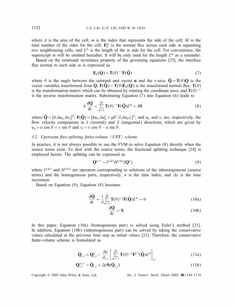
Figure 4. Comparisons of exact solutions with simulated depths using rst-orderschemes for a water depth ratio hd=hu of 0.5.

0

2

4

6

8

10

12

0 400 800 1200 1600 2000

Distance (m)

Dep

th (

m)

ExactUFFOsherRoeHLL

9.40

9.75

10.10

400 450 500 550

3.3

4.4

5.5

800 1000 1200

0

1

2

1500 1600 1700

UFF

Osher

Roe

× HLL

Figure 5. Comparisons of exact solutions with simulated depths using rst-orderschemes for a water depth ratio hd=hu of 0.01.

simulation time is 50 s for test cases with water depth ratios of 0.5 and 0.01. For the testcase with dry bed condition, the simulation time is 30 s after dam break. The exact solutionscan be found in Reference [26].



0

2

4

6

8

10

12

0 400 800 1200 1600 2000

Distance (m)

Dep

th (

m)

ExactUFFOsherRoeHLL

9.40

9.75

10.10

630 680 730

3.3

4.4

5.5

900 1000 1100

0

1

1300 1400 1500

UFF

Osher

Roe

× HLL

Figure 6. Comparisons of exact solutions with simulated depths using rst-orderschemes for a water depth ratio hd=hu of 0.

Comparison of the exact solutions with the simulated water depths using the four rst-orderupwind schemes for a water depth ratio of 0.5 is shown in Figure 4. As shown in Figure 4with the close-up of the shock wave front as well as the head of the rarefaction wave, allschemes provide solutions without any spurious oscillations. The Osher scheme presents themost accurate solution of the shock wave front, whereas the HLL scheme yields more diusiveresults. Among the schemes tested, the proposed UFF scheme has the best resolution of thehead of the rarefaction wave.For the test case with a water depth ratio of 0.01, as shown in Figure 5, the Roe scheme

produces the expansion shock at the dam site, whereas the UFF, Osher and HLL schemes donot. Hence, the formula of entropy correction given by Harten and Hyman [1] is employedfor the Roe scheme afterward. Results of comparisons in this test case are similar to thosein the previous test case for the resolution of the shock front and the head of the rarefactionwave. The simulated results at the dam site also show that the UFF scheme produces the bestresolution. Unlike the Roe scheme, the UFF scheme satisfying entropy condition can resolvethe rarefaction wave smoothly at the dam site. For the test case with dry bed condition, asshown in Figure 6, the UFF scheme gives the best resolutions of the rarefaction wave at thedam site as well as at the head. The simulated wet=dry front by the UFF scheme ts the exactsolution much more smoothly and closely than that by other presented schemes.To show the inuence of the CFL number on the simulated results, dierent CFL numbers

are considered herein with xed cell size of 20m. Using the rst-order UFF scheme, Figure 7shows the inuence of the CFL number on the simulated water depth for the test case withthe water depth ratio hd=hu of 0.01. It is clear that the proposed scheme do not produceoscillations in the solutions even if the CFL number equals one. In addition, the scheme witha higher CFL can achieve better resolution of the shock front.



0

2

4

6

8

10

12

0 400 800 1200 1600 2000

Distance (m)

Dep

th (

m)

Exact

CFL = 1.0

CFL = 0.8

CFL = 0.6

CFL = 0.4

0

1

2

1500 1600 1700

CFL = 1.0

CFL = 0.8

CFL = 0.6

× CFL = 0.4

Figure 7. The inuence of the CFL number on the simulated water depth using the rst-order UFFscheme for the water depth ratio hd=hu of 0.01.

To evaluate the numerical accuracy quantitatively, two dierent error norms, L2 (overallerror norm) and L∞ (max error norm), are used herein [27].

L2 =

√∑(Y simi; j − Y exacti; j )2∑(Y exacti; j )2

; L∞=max |Y simi; j − Y exacti; j |max |Y exacti; j | (35)

where Y simi; j and Y exacti; j are the simulated solution and the exact solution at cell (i; j), respec-tively. Table I summarizes the error norms of the water depth and CPU time for water depthratios of 0:5; 0:01 and 0. The results show that the proposed UFF scheme yields the smallestL2 norm of water depth, whereas the HLL scheme gives the largest those. As listed in Ta-ble I, for the test cases with water depth ratios of 0.5 and 0.01, the values of the L∞ normsindicate that the Osher scheme presents better solutions near the shock front. Nevertheless,for the test case with dry bed condition downstream, the UFF scheme performs the mostaccurate solutions in the entire simulation domain. Accordingly, the UFF scheme consumesthe shortest CPU time, whereas the Roe scheme takes the longest one.Based on the analyses of the above tested cases, the UFF scheme can avoid the entropy-

violating solution and it resolves rarefaction wave more smoothly as well as accurately at thedam site. Although the Osher scheme performs better solutions near the shock front locallyreferring to the smallest L∞ in Table I for the test cases with water depth ratios of 0.5 and0.01, the proposed UFF scheme achieves superior overall numerical accuracy and eciencyamong the schemes tested. Furthermore, the UFF scheme can simulate the wet=dry wave frontpassing over a dry bed condition downstream well.



Table I. Simulated results for the 1D idealized dam-break problem using rst-order schemes.

hd=hu = 0:5 hd=hu = 0:01 hd=hu = 0

Schemes L2 L∞ CPU (s) L2 L∞ CPU (s) L2 L∞ CPU (s)

UFF 0.0155 0.0695 0.058 0.0319 0.1612 0.076 0.0168 0.0474 0.045

Osher 0.0158 0.0619 0.077 0.0321 0.1392 0.101 0.0233 0.0539 0.061Roe 0.0169 0.0688 0.102 0.0361 0.1612 0.136 0.0259 0.0561 0.079HLL 0.0212 0.0825 0.071 0.0406 0.1629 0.091 0.0326 0.0656 0.055

Shock front

O

Figure 8. The plan view of the oblique shock front.

4.2. Oblique hydraulic jump

When a converging vertical boundary is deected along the channel contraction through anangle inward the supercritical ow, an oblique hydraulic jump originating at point O canbe formed with an angle of as shown in Figure 8. This test problem in steady supercriticalow has been commonly adopted and simulated by researchers [8, 11, 12, 15, 16, 20, 21]. In theconverging channel with zero bed slope, the angle between the converging wall and the owdirection is taken as =8:95. Figure 9 shows the geometry and the computational mesh, inwhich 80× 60 non-rectangular cells are used. The initial conditions corresponding to a Froudenumber of 2.74 are given by: the water depth of 1 m, the velocity component u of 8:57 m=sand v of zero. At the upstream inow boundary, the supercritical inow boundary conditionsof h=1m, u=8:57m=s and v=0m=s are imposed. The transmissive boundary conditions aregiven using Equation (34) at the downstream outow boundary. The computational time stepis taken as 0:02 s. To obtain a steady-state solution, a convergence criterion in terms of therelative error R is dened as

R=

√∑(hn+1i; j − hni; j)2∑(hni; j)2

61:0× 10−5 (36)

where hni; j and hn+1i; j are the local water depths at the time steps n and n+ 1, respectively.

Figure 10 shows the comparison between the exact solutions and the simulated water depthsusing the UFF, Osher, Roe and HLL schemes along line EGH illustrated in Figure 9. The



x (m)

y (m

)

0 10 20 30 400

5

10

15

20

25

30

EG

H

Figure 9. The geometry and the computational mesh for the 2D oblique hydraulic jump problem.

0.9

1.0

1.1

1.2

1.3

1.4

1.5

1.6

0 5 10 15 20 25 30 35 40

Distance (m)

Dep

th (

m)

Exact

UFF

Osher

Roe

HLL

1.15

1.18

1.20

23.0 23.5 24.0

Figure 10. Comparisons of the exact solutions with the simulated water depth proles along line EGH(see Figure 9) using rst-order schemes.

exact solutions can be found in Reference [28]. As shown in Figure 10, the oblique hydraulicjump is captured well by all schemes. However, from the close-up near the shock front shownin Figure 10, the proposed UFF scheme even resolves the jump slightly sharper than the otherschemes.



Table II. Simulated results for the oblique hydraulic jump problem using rst-order schemes.

CPU time forL2 norm of shock convergence criterion

Scheme L2 norm of depth L2 norm of velocity angle (s)

UFF 0.035 0.0058 0.0030 15.63

Osher 0.037 0.0061 0.0036 21.02Roe 0.039 0.0063 0.0042 29.05HLL 0.041 0.0068 0.0044 19.26

Contour interval = 0.05 m

5 10 15 20 25 30 35

x (m)

5 10 15 20 25 30 35

x (m)

5

10

15

20

25

y (m

)

5

10

15

20

25

y (m

)

Contour interval = 0.05 m

(b)(a)

Figure 11. The contour plots of the 2D oblique hydraulic jump using: (a) UFF; and(b) UFF-MUSCL schemes.

Table II lists the simulated results, including the L2 norms of water depth, velocity, andshock angle. The CPU time for reaching the convergence criterion is also presented in Table II.It is found that the proposed UFF scheme has the best numerical accuracy and eciency. Inaddition, Figures 11(a) and 11(b) show the simulated water depth contours of the steadystate solutions using the UFF and UFF-MUSCL schemes, respectively. The simulated resultsshow no oscillations produced for both schemes. Certainly, the second-order UFF-MUSCLscheme presents a better resolution than the rst-order UFF scheme. From the simulated resultspresented above, we may conclude that the UFF scheme has the best numerical performancein modelling the 2D oblique hydraulic jump problem.

4.3. Circular dam-break ow

This problem is designed to test the capability of the proposed scheme in modelling 2Dsymmetric discontinuous free surfaces. Numerical results for this test problem can be foundin References [8, 11, 14, 21]. Figure 12 shows the geometry, in which a cylindrical damwith radius 11 m is located in the middle of the computational domain. The circular mesh(Figure 13) consisting of 50 cells in the tangential direction and 25 cells of 1m length alongthe radial direction is employed herein.



(-25, 25) (25, 25)

(-25, -25) (25, -25)

Circular dam

x (m)

y (m

)

r = 11 m

Figure 12. The geometry for the 2D circular dam-break problem.

x (m)

y (m

)

-20 -10 0 10 20

-20

-10

0

10

20

S T

Figure 13. The computational mesh for the 2D circular dam-break problem.



0

2

4

6

8

10

0 5 10 15 20 25

Distance (m)

0 5 10 15 20 25

Distance (m)

Dep

th (

m)

UFFOsherRoeHLLDam site

4

5

6

10.0 10.5 11.0 11.5 12.0

0

1

2

Frou

de n

umbe

r

UFFOsherRoeHLLDam site

0.50

0.60

0.70

0.80

0.90

1.00

1.10

1.20

10 10.5 11 11.5 12

(a)

(b)

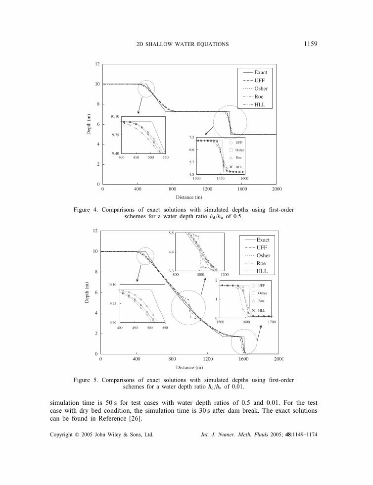
Figure 14. Comparisons of the: (a) simulated water depth proles; and (b) Froude numbers along lineST (see Figure 13) using rst-order schemes.

The initial condition comprises two regions of still water depth separated by the cylin-drical dam, at which water depth inside the dam is 10 m and outside the dam is 1 m. Thecomputational time step is 0:02 s. Figures 14(a) and 14(b) show, respectively, the simulatedwater depths and the Froude numbers using all presented rst-order schemes along line ST att=0:69 s. The results show that the Osher and the Roe schemes produce signicant glitchesat the dam site whereas the proposed UFF and the HLL schemes do not. The glitch standsfor the disadvantage of the Osher and the Roe schemes whereas the solution at the dam siteshould be a smooth water surface prole for rarefaction wave. Besides, the ow at the damsite is the critical ow [24], i.e. the exact solution of the Froude number (NF) should beequal to one, which is very useful for comparison. From the close-up view of dam site inFigure 14(b), the simulated Froude number by the proposed UFF scheme produces the closestvalue to the exact solution (i.e. NF =1). On the other hand, the CPU time required is 10:52 s



-20 -15 -10 -5 0 5 10 15 20

x (m)

-20

-15

-10

-5

0

5

10

15

20

y (m

)

2

4

6

8

10

h(m

)

-20-10

010

20

x (m)-20

-100

1020 y (m)

X

Y

ZC

onto

ur in

terv

al =

0.7

m

(a) (b)

Figure 15. (a) The 2D contour plot; and (b) 3D free-surface view showing water depth variations forthe circular dam breaking at t=0:69 s using the UFF-MUSCL scheme.

Table III. Inuence of the computational mesh on the simulated Froude number at the damsite for 2D circular dam-break problem.

Number of cells in Number of cells inthe tangential the radial

Mesh direction direction UFF Osher Roe HLL

M1 50 25 0.815 0.731 0.705 0.762M2 100 50 0.892 0.841 0.831 0.857M3 200 100 0.935 0.905 0.905 0.911M4 300 150 0.965 0.942 0.938 0.956M5 400 200 0.985 0.972 0.971 0.981

for the UFF scheme. The ratios of the CPU time consumed by the Osher, Roe and HLLschemes to that required by the UFF scheme are 1:25; 1:82, and 1.36, respectively. From theabove comparisons, it is found that the UFF scheme is the most accurate and ecient amongthe schemes presented.The 2D contour as well as the 3D view of the water surface elevation at t=0:69s computed

by the second-order UFF-MUSCL scheme are shown in Figures 15(a) and 15(b), respectively.The simulated results show that there is an outward-propagating circular shock wave and aninward-propagating circular rarefaction wave. The perfect symmetric ow behaviour agreesvery well with those found in References [8, 11, 14, 21].To further demonstrate the numerical performance of the proposed UFF scheme, a grid

convergence study known as the grid renement study is performed herein [29]. Five dierent



0

1

2

0 5 10 15 20 25

Distance (m)

Fro

ud

e n

um

ber

M1

M2

M3

M4

M5

Dam site

0.6

0.7

0.8

0.9

1.0

1.1

1.2

10.0 10.5 11.0 11.5 12.0

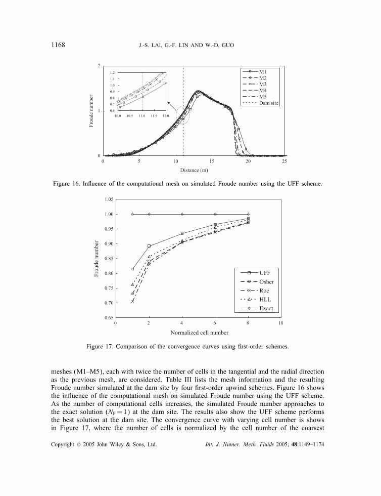
Figure 16. Inuence of the computational mesh on simulated Froude number using the UFF scheme.

0.65

0.70

0.75

0.80

0.85

0.90

0.95

1.00

1.05

0 2 4 6 8 10

Normalized cell number

Fro

ude

num

ber

UFF

Osher

Roe

HLL

Exact

Figure 17. Comparison of the convergence curves using rst-order schemes.

meshes (M1–M5), each with twice the number of cells in the tangential and the radial directionas the previous mesh, are considered. Table III lists the mesh information and the resultingFroude number simulated at the dam site by four rst-order upwind schemes. Figure 16 showsthe inuence of the computational mesh on simulated Froude number using the UFF scheme.As the number of computational cells increases, the simulated Froude number approaches tothe exact solution (NF =1) at the dam site. The results also show the UFF scheme performsthe best solution at the dam site. The convergence curve with varying cell number is showsin Figure 17, where the number of cells is normalized by the cell number of the coarsest



mesh (M1). Each solution is properly converged with respect to iterations and an almost meshindependent solution (i.e. NF =1) is achieved using the UFF scheme with the M5 mesh.

4.4. Dam-break experiment with 45 bend channel

This section tests the capability of the proposed UFF and its second-order extension UFF-MUSCL scheme in modelling 2D dam-break ow over a channel with a 45 bend. Thedam-break experiment with a 45 bend channel was carried out by Sorares et al. [30] at theCatholic University of Louvain, Belgium; more details can be found in Toro’s book [24]. Theexperimental domain consists of a rectangular reservoir connected to a channel containing a45 bend, as shown in Figure 18.Both the reservoir and the channel are horizontal and connected by a dam. The geometry

of the experiment layout and the locations of the observation stations in the physical modelare given in Figure 18. The initial water depths are 0:25m in the reservoir and 0:01m in thechannel. The total simulation time is 45s after dam break. Manning’s roughness coecient nmfor bed friction is calibrated to be 0.011. The computational mesh with 3950 non-rectangularcells is used.Using the UFF scheme and its second-order UFF-MUSCL scheme, the comparisons of

the simulated water depth hydrographs with the experimental data at dierent observation

x (m)

y(m

)

10

1

9

2

8

3

7

4

5

6

Dam

G1 G2 G3 G4G5G6

G7

G8

G9

Point number x (m) y (m) Observations x(m) y (m)

1 0.0 0.0 G1 1.59 0.69

2 2.39 0.0 G2 2.74 0.69

3 2.39 0.445 G3 4.24 0.69

4 6.64 0.445 G4 5.74 0.69

5 9.575 3.38 G5 6.74 0.72

6 9.225 3.73 G6 6.65 0.80

7 6.435 0.94 G7 6.56 0.89

8 2.39 0.94 G8 7.07 1.22

9 2.39 2.44 G9 8.13 2.28

10 0.0 2.44

Figure 18. The layout of the dam-break experiment with 45 bend channel.



0.00

0.05

0.10

0.15

0.20

0.25

0 5 10 15 20 25 30 35 40

Time (s)

0 5 10 15 20 25 30 35 40

Time (s)

0 5 10 15 20 25 30 35 40

Time (s)

0 5 10 15 20 25 30 35 40

Time (s)

0 5 10 15 20 25 30 35 40

Time (s)

0 5 10 15 20 25 30 35 40

Time (s)

0 5 10 15 20 25 30 35 40

Time (s)

0 5 10 15 20 25 30 35 40

Time (s)

0 5 10 15 20 25 30 35 40

Time (s)

Dep

th (

m)

0.00

0.05

0.10

0.15

0.20

0.25

Dep

th (

m)

0.00

0.05

0.10

0.15

0.20

0.25

Dep

th (

m)

0.00

0.05

0.10

0.15

0.20

0.25

Dep

th (

m)

0.00

0.05

0.10

0.15

0.20

0.25

Dep

th (

m)

0.00

0.05

0.10

0.15

0.20

0.25

Dep

th (

m)

0.00

0.05

0.10

0.15

0.20

0.25

Dep

th (

m)

0.00

0.05

0.10

0.15

0.20

0.25

Dep

th (

m)

0.00

0.05

0.10

0.15

0.20

0.25

Dep

th (

m)

MeasuredUFFUFF-MUSCL

Measured

UFF

UFF-MUSCL


Measured

UFFUFF-MUSCL





Measured

UFFUFF-MUSCL

(a) (b)

(c) (d)

(e) (f )

(g) (h)

(i)

Figure 19. Comparisons of the measured and simulated water depths against time at Station:(a) G1; (b) G2; (c) G3; (d) G4; (e) G5; (f) G6; (g) G7; (h) G8; and (i) G9 for the

dam-break experiment with 45 bend channel.



0

0.1

0.2

h(m

)

01

23

45

67

89

x (m)01

23

y (m)

X Y

Z

0.25

0.24

0.22

0.01

x (m)

y(m

)

1 2 3 4 5 6 7 8 9

0.5

1

1.5

2

2.5

3

3.5

4

(a)

(b)

Figure 20. The simulated: (a) 2D contour plot; and (b) 3D free-surface view showing water depthvariations for the dam-break experiment at t=0:5 s by the UFF-MUSCL scheme.

stations are made in Figure 19. The results show shock waves propagating toward downstreamchannel and reecting on the channel bend boundaries. The rarefaction wave travels into thereservoir. For all observation stations shown in Figure 19, the simulated water depths agreewell with the measured. Although experimental data give remarkable oscillatory behaviours,the UFF and its second-order extension UFF-MUSCL schemes present satisfactory overallsolutions. Obviously, the simulated results of the reections from the bend by the UFF-MUSCL scheme are better captured, while the UFF scheme gives smoother solutions, typicallyshown in Figures 19(b), 19(c) and 19(d) for observation stations G2;G3 and G4, respectively.The simulated 2D contour plot and 3D free-surface view showing water depth variations att=0:5 s using the UFF-MUSCL scheme are shown in Figures 20(a) and 20(b), respectively.



0

0.1

0.2

h(m

)

01

23

45

67

89

x (m)01

23

y (m)

X Y

Z

0.20

0.19

0.100.10

0.09

0.01

0.15

x (m)

y(m

)

1 2 3 4 5 6 7 8 9

0.5

1

1.5

2

2.5

3

3.5

4

(a)

(b)

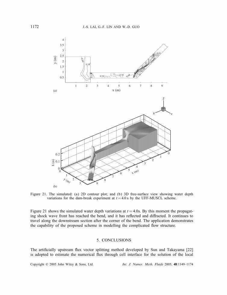
Figure 21. The simulated: (a) 2D contour plot; and (b) 3D free-surface view showing water depthvariations for the dam-break experiment at t=4:0 s by the UFF-MUSCL scheme.

Figure 21 shows the simulated water depth variations at t=4:0s. By this moment the propagat-ing shock wave front has reached the bend, and it has reected and diracted. It continues totravel along the downstream section after the corner of the bend. The application demonstratesthe capability of the proposed scheme in modelling the complicated ow structure.

5. CONCLUSIONS

The articially upstream ux vector splitting method developed by Sun and Takayama [22]is adopted to estimate the numerical ux through cell interface for the solution of the local



Riemann problem. By applying the corresponding numerical ux function, the upstream ux-splitting nite-volume (UFF) scheme is proposed for solving the 2D SWE in the framework ofthe FVM. The MUSCL method and the predictor–corrector approach are employed to achievethe second-order-accurate extension in space and in time, respectively.The numerical performance of the proposed UFF scheme is compared with those of the

Osher, Roe and HLL schemes for the 1D idealized dam break, 2D steady oblique hydraulicjump and 2D circular dam-break problems. Based on the simulated results of the 1D idealizeddam-break problem, it is found that the UFF scheme presents superior overall numericalaccuracy as well as eciency because it produces the least L2 error norm and consumes thesmallest CPU time. Due to satisfaction of the entropy condition, the UFF scheme can resolverarefaction wave smoothly and accurately at the dam site. Furthermore, the UFF scheme cansimulate the wet=dry wave front passing over a dry bed condition downstream well.According to the simulated results of the 2D oblique hydraulic jump problem, the UFF

scheme also obtains superior overall numerical performances among the schemes tested. Fromthe simulated results of the 2D circular dam-break problem, the UFF scheme presents thebest numerical eciency and provides good agreement with the results reported by otherresearchers [8, 11, 14, 21]. A grid convergence study is also tested for the 2D circular dam-break problem to conclude that the UFF scheme performs the best solution at the dam site.Moreover, the applications of the UFF and UFF-MUSCL schemes to the dam-break experi-ment with a 45 bend channel demonstrate the capability and reliability of dam-break owsimulation. From the above analyses, the proposed schemes are simple, accurate, ecient andsuitable for modelling shallow water ows containing discontinuities.

REFERENCES

1. Hirsch C. Numerical Computation of Internal and External Flows, vol. 2. Wiley: Chichester, 1990.2. Toro EF. Riemann Solvers and Numerical Methods for Fluid Dynamics. Springer: Berlin, 1997.3. Roe PL. Approximate Riemann solvers, parameter vectors, and dierence schemes. Journal of ComputationalPhysics 1981; 43:357–372.

4. Osher S, Solomone F. Upwind dierence schemes for hyperbolic systems of conservation laws. Mathematicsand Computers in Simulation 1982; 38:339–374.

5. Steger JL, Warming RF. Flux vector splitting of the inviscid gas dynamic equations with application to nitedierence methods. Journal of Computational Physics 1981; 40:263–293.

6. Zhao DH, Shen HW, Tabios GQ, Lai JS, Tan WY. Finite-volume two-dimensional unsteady-ow model owriver basins. Journal of Hydraulic Engineering 1994; 120(12):863–882.

7. Wan Q, Wan H, Zhou C, Wu Y. Simulating the hydraulic characteristics of the lower Yellow River by thenite-volume technique. Hydrological Processes 2002; 16(14):2767–2769.

8. Alcrudo F, Garcia-Navarro P. A high-resolution Godunov-type scheme in nite volumes for the 2D shallowwater equations. International Journal for Numerical Methods in Fluids 1993; 16:489–505.

9. Anastasiou K, Chan CT. Solution of the 2D shallow water equations using the nite volume method onunstructured triangular meshes. International Journal for Numerical Methods in Fluids 1997; 24:1225–1245.

10. Sleigh PA, Gaskell PH, Berzins M, Wright NG. An unstructured nite-volume algorithm for predicting ow inrivers and estuaries. Computers and Fluids 1998; 27(4):479–508.

11. Tseng MH. Explicit nite volume non-oscillatory schemes for 2D transient free-surface ows. InternationalJournal for Numerical Methods in Fluids 1999; 30:831–843.

12. Tseng MH, Chu CR. Two-dimensional shallow water ows simulation using TVD-MacCormack scheme. Journalof Hydraulic Research 2000; 38(2):123–131.

13. Brufau P, Garcia-Navarro P. Two-dimensional dam break ow simulation. International Journal for NumericalMethods in Fluids 2000; 33:35–57.

14. Mingham CG, Causon DM. High-resolution nite-volume method for shallow water ows. Journal of HydraulicEngineering 1998; 124(6):605–614.

15. Hu K, Mingham CG, Causon DM. A bore-capturing nite volume method for open-channel ows. InternationalJournal for Numerical Methods in Fluids 1998; 28:1241–1261.



16. Causon DM, Mingham CG, Ingram DM. Advances in calculation methods for supercritical ow in spillwaychannels. Journal of Hydraulic Engineering 1999; 125(10):1039–1050.

17. Valiani A, Cale V, Zanni A. Case study: Malpasset Dam-break simulation using a two-dimensional nitevolume method. Journal of Hydraulic Engineering 2002; 28(5):460–472.

18. Zoppou C, Roberts S. Catastrophic collapse of water supply reservoirs in urban areas. Journal of HydraulicEngineering 1999; 125(7):686–695.

19. Zhao DH, Shen HW, Lai JS, Tabios GQ. Approximate Riemann solvers in FVM for 2D hydraulic shock wavemodeling. Journal of Hydraulic Engineering 1996; 122(12):692–702.

20. Lin GF, Lai JS, Guo WD. Finite-volume component-wise TVD schemes for 2D shallow water equations.Advances in Water Resources 2003; 26(8):861–873.

21. Erduran KS, Kutija V, Hewett CJM. Performance of nite volume solutions to the shallow water equations withshock-capturing schemes. International Journal for Numerical Methods in Fluids 2002; 40:1237–1273.

22. Sun M, Takayama K. An articially upstream ux vector splitting scheme for the Euler equations. Journal ofComputational Physics 2003; 189:305–329.

23. Tan WY. Shallow Water Hydrodynamics. Elsevier: New York, 1992.24. Toro EF. Shock-capturing Methods for Free-surface Shallow Water Flows. Wiley: New York, 2001.25. Wada Y, Lious MS. An accurate and robust ux splitting scheme for shock and contact discontinuities. SIAM

Journal on Scientic Computing 1997; 18(3):633–657.26. Stoker JJ. Water Waves: Mathematical Theory with Applications. Wiley-Interscience: Singapore, 1958.27. LeVeque RJ. Finite Volume Methods for Hyperbolic Problems. Cambridge University Press: Cambridge, U.K.,

2002.28. Hager WH, Schwalt M, Jimenez O, Chaudry MH. Supercritical ow near an abrupt wall deection. Journal of

Hydraulic Research 1994; 32(1):103–118.29. Roache PJ. Verication and Validation in Computational Science and Engineering. Hermosa Publishers:

Albuquerque, New Mexico, 1998.30. Sorares S, Sillen X, Zech Y. Dam-break ow through sharp bends. Physical models and 2d boltzmann model

validation. European Commission, IBSN 92-828-7108-8, 1999.


anupstreamux-splittingnite-volumeschemefor2d...

Documents