anywhere-anytime signalsandsystemslaboratory · anywhere-anytime signalsandsystemslaboratory...

Anywhere-AnytimeSignals and Systems LaboratoryFromMATLAB to Smartphones

Synthesis Lectures on SignalProcessing

EditorJoséMoura,CarnegieMellon University

Synthesis Lectures in Signal Processing publishes 80- to 150-page books on topics of interest tosignal processing engineers and researchers. e Lectures exploit in detail a focused topic. ey canbe at different levels of exposition-from a basic introductory tutorial to an advancedmonograph-depending on the subject and the goals of the author. Over time, the Lectures willprovide a comprehensive treatment of signal processing. Because of its format, the Lectures will alsoprovide current coverage of signal processing, and existing Lectures will be updated by authors whenjustified.Lectures in Signal Processing are open to all relevant areas in signal processing. ey will covertheory and theoretical methods, algorithms, performance analysis, and applications. Some Lectureswill provide a new look at a well established area or problem, while others will venture into a brandnew topic in signal processing. By careful reviewing the manuscripts we will strive for quality both inthe Lectures’ contents and exposition.

Anywhere-Anytime Signals and Systems Laboratory: From MATLAB to SmartphonesNasser Kehtarnavaz and Fatemeh Saki2016

Smartphone-Based Real-Time Digital Signal ProcessingNasser Kehtarnavaz, Shane Parris, and Abhishek Sehgal2015

An Introduction to Kalman Filtering with MATLAB ExamplesNarayan Kovvali, Mahesh Banavar, and Andreas Spanias2013

Sequential Monte Carlo Methods for Nonlinear Discrete-Time FilteringMarcelo G.S. Bruno2013

Processing of Seismic Reflection Data Using MATLAB™Wail A. Mousa and Abdullatif A. Al-Shuhail2011

iii

Fixed-Point Signal ProcessingWayne T. Padgett and David V. Anderson2009

Advanced Radar Detection Schemes Under Mismatched Signal ModelsFrancesco Bandiera, Danilo Orlando, and Giuseppe Ricci2009

DSP for MATLAB™ and LabVIEW™ IV: LMS Adaptive FilteringForester W. Isen2009

DSP for MATLAB™ and LabVIEW™ III: Digital Filter DesignForester W. Isen2008

DSP for MATLAB™ and LabVIEW™ II: Discrete Frequency TransformsForester W. Isen2008

DSP for MATLAB™ and LabVIEW™ I: Fundamentals of Discrete Signal ProcessingForester W. Isen2008

e eory of Linear PredictionP. P. Vaidyanathan2007

Nonlinear Source SeparationLuis B. Almeida2006

Spectral Analysis of Signals: e Missing Data CaseYanwei Wang, Jian Li, and Petre Stoica2006

Copyright © 2017 by Morgan & Claypool

All rights reserved. No part of this publication may be reproduced, stored in a retrieval system, or transmitted inany form or by any means—electronic, mechanical, photocopy, recording, or any other except for brief quotationsin printed reviews, without the prior permission of the publisher.

Anywhere-Anytime Signals and Systems Laboratory: From MATLAB to Smartphones

Nasser Kehtarnavaz and Fatemeh Saki

www.morganclaypool.com

ISBN: 9781627059015 paperbackISBN: 9781627055031 ebook

DOI 10.2200/S00727ED1V01Y201608SPR014

A Publication in the Morgan & Claypool Publishers seriesSYNTHESIS LECTURES ON SIGNAL PROCESSING

Lecture #14Series Editor: José Moura, Carnegie Mellon UniversitySeries ISSNPrint 1932-1236 Electronic 1932-1694

www.morganclaypool.com

Anywhere-AnytimeSignals and Systems LaboratoryFromMATLAB to Smartphones

Nasser Kehtarnavaz and Fatemeh SakiUniversity of Texas at Dallas

SYNTHESIS LECTURES ON SIGNAL PROCESSING #14

CM&

cLaypoolMorgan publishers&

ABSTRACTA typical undergraduate electrical engineering curriculum incorporates a signals and systemscourse. e widely used approach for the laboratory component of such courses involves the uti-lization of MATLAB to implement signals and systems concepts. is book presents a newlydeveloped laboratory paradigm where MATLAB codes are made to run on smartphones, whichmost students already possess. is smartphone-based approach enables an anywhere-anytimeplatform for students to conduct signals and systems experiments. is book covers the labo-ratory experiments that are normally covered in signals and systems courses and discusses howto run MATLAB codes for these experiments on smartphones, thus enabling a truly mobilelaboratory environment for students to learn the implementation aspects of signals and sys-tems concepts. A zipped file of the codes discussed in the book can be acquired via the websitehttp://sites.fastspring.com/bookcodes/product/SignalsSystemsBookcodes.

KEYWORDSsmartphone-based signals and systems laboratory; anywhere-anytime platform forsignals and system courses; from MATLAB to smartphones

http://sites.fastspring.com/bookcodes/product/SignalsSystemsBookcodes

vii

ContentsPreface . . . . . . . . . . . . . . . . . . . . . . . . . . . . . . . . . . . . . . . . . . . . . . . . . . . . . . . . . . . . xi

1 Introduction toMATLAB . . . . . . . . . . . . . . . . . . . . . . . . . . . . . . . . . . . . . . . . . . . . 1

1.1 Starting MATLAB . . . . . . . . . . . . . . . . . . . . . . . . . . . . . . . . . . . . . . . . . . . . . . . . 11.1.1 Arithmetic Operations . . . . . . . . . . . . . . . . . . . . . . . . . . . . . . . . . . . . . . . . 11.1.2 Vector Operations . . . . . . . . . . . . . . . . . . . . . . . . . . . . . . . . . . . . . . . . . . . . 51.1.3 Complex Numbers . . . . . . . . . . . . . . . . . . . . . . . . . . . . . . . . . . . . . . . . . . . 61.1.4 Array Indexing . . . . . . . . . . . . . . . . . . . . . . . . . . . . . . . . . . . . . . . . . . . . . . 71.1.5 Allocating Memory . . . . . . . . . . . . . . . . . . . . . . . . . . . . . . . . . . . . . . . . . . . 81.1.6 Special Characters and Functions . . . . . . . . . . . . . . . . . . . . . . . . . . . . . . . . 91.1.7 Control Flow . . . . . . . . . . . . . . . . . . . . . . . . . . . . . . . . . . . . . . . . . . . . . . . 101.1.8 Programming in MATLAB . . . . . . . . . . . . . . . . . . . . . . . . . . . . . . . . . . . 121.1.9 Sound Generation . . . . . . . . . . . . . . . . . . . . . . . . . . . . . . . . . . . . . . . . . . . 131.1.10 Loading and Saving Data . . . . . . . . . . . . . . . . . . . . . . . . . . . . . . . . . . . . . 141.1.11 Reading Wave and Image Files . . . . . . . . . . . . . . . . . . . . . . . . . . . . . . . . . 141.1.12 Signal Display . . . . . . . . . . . . . . . . . . . . . . . . . . . . . . . . . . . . . . . . . . . . . . 15

1.2 MATLAB Programming Examples . . . . . . . . . . . . . . . . . . . . . . . . . . . . . . . . . . 151.2.1 Signal Generation . . . . . . . . . . . . . . . . . . . . . . . . . . . . . . . . . . . . . . . . . . . 151.2.2 Generating a Periodic Signal . . . . . . . . . . . . . . . . . . . . . . . . . . . . . . . . . . 17

1.3 Lab Exercises . . . . . . . . . . . . . . . . . . . . . . . . . . . . . . . . . . . . . . . . . . . . . . . . . . . . 18

2 Android Software Development Tools . . . . . . . . . . . . . . . . . . . . . . . . . . . . . . . . . 21

2.1 Installation Steps . . . . . . . . . . . . . . . . . . . . . . . . . . . . . . . . . . . . . . . . . . . . . . . . . 212.1.1 Java JDK . . . . . . . . . . . . . . . . . . . . . . . . . . . . . . . . . . . . . . . . . . . . . . . . . . 212.1.2 Android Studio Bundle and Native Development Kit . . . . . . . . . . . . . . . 222.1.3 Environment Variable Configuration . . . . . . . . . . . . . . . . . . . . . . . . . . . . 232.1.4 Android Studio Configuration . . . . . . . . . . . . . . . . . . . . . . . . . . . . . . . . . 242.1.5 Android Emulator Configuration . . . . . . . . . . . . . . . . . . . . . . . . . . . . . . . 27

2.2 Getting Familiar with Android Software Tools . . . . . . . . . . . . . . . . . . . . . . . . . . 31

viii

3 FromMATLABCoder to Smartphone . . . . . . . . . . . . . . . . . . . . . . . . . . . . . . . . 433.1 MATLAB Function Design . . . . . . . . . . . . . . . . . . . . . . . . . . . . . . . . . . . . . . . . 433.2 Generating Signals via MATLAB on Smartphones . . . . . . . . . . . . . . . . . . . . . . 45

3.2.1 Test Bench . . . . . . . . . . . . . . . . . . . . . . . . . . . . . . . . . . . . . . . . . . . . . . . . . 463.2.2 C Code Generation . . . . . . . . . . . . . . . . . . . . . . . . . . . . . . . . . . . . . . . . . . 463.2.3 Source Code Integration . . . . . . . . . . . . . . . . . . . . . . . . . . . . . . . . . . . . . . 48

3.3 Running MATLAB Coder C Codes on Smartphones . . . . . . . . . . . . . . . . . . . . 523.4 References . . . . . . . . . . . . . . . . . . . . . . . . . . . . . . . . . . . . . . . . . . . . . . . . . . . . . . . 56

4 Linear Time-Invariant Systems and Convolution . . . . . . . . . . . . . . . . . . . . . . . . 574.1 Convolution and Its Numerical Approximation . . . . . . . . . . . . . . . . . . . . . . . . . 574.2 Convolution Properties . . . . . . . . . . . . . . . . . . . . . . . . . . . . . . . . . . . . . . . . . . . . 594.3 Convolution Experiments . . . . . . . . . . . . . . . . . . . . . . . . . . . . . . . . . . . . . . . . . . 594.4 Lab Exercises . . . . . . . . . . . . . . . . . . . . . . . . . . . . . . . . . . . . . . . . . . . . . . . . . . . . 89

4.4.1 Echo Cancellation . . . . . . . . . . . . . . . . . . . . . . . . . . . . . . . . . . . . . . . . . . . 894.4.2 Noise Reduction Using Mean Filtering . . . . . . . . . . . . . . . . . . . . . . . . . . 904.4.3 Impulse Noise Reduction Using Median Filtering . . . . . . . . . . . . . . . . . . 91

4.5 Running MATLAB Coder C Codes on Smartphone . . . . . . . . . . . . . . . . . . . . 914.6 Running in Real-Time on Smartphones . . . . . . . . . . . . . . . . . . . . . . . . . . . . . . . 95

4.6.1 MATLAB Function Design . . . . . . . . . . . . . . . . . . . . . . . . . . . . . . . . . . . 954.6.2 Test Bench . . . . . . . . . . . . . . . . . . . . . . . . . . . . . . . . . . . . . . . . . . . . . . . . . 954.6.3 Modifying a Real Time Shell . . . . . . . . . . . . . . . . . . . . . . . . . . . . . . . . . . 99

4.7 References . . . . . . . . . . . . . . . . . . . . . . . . . . . . . . . . . . . . . . . . . . . . . . . . . . . . . . 105

5 Fourier Series . . . . . . . . . . . . . . . . . . . . . . . . . . . . . . . . . . . . . . . . . . . . . . . . . . . . 1075.1 Fourier Series Numerical Computation . . . . . . . . . . . . . . . . . . . . . . . . . . . . . . . 1085.2 Fourier Series and Its Applications . . . . . . . . . . . . . . . . . . . . . . . . . . . . . . . . . . 1095.3 Lab Exercises . . . . . . . . . . . . . . . . . . . . . . . . . . . . . . . . . . . . . . . . . . . . . . . . . . . 123

5.3.1 RL Circuit Analysis . . . . . . . . . . . . . . . . . . . . . . . . . . . . . . . . . . . . . . . . 1235.3.2 e Doppler Effect . . . . . . . . . . . . . . . . . . . . . . . . . . . . . . . . . . . . . . . . . 1245.3.3 Synthesis of Electronic Music . . . . . . . . . . . . . . . . . . . . . . . . . . . . . . . . . 124

5.4 References . . . . . . . . . . . . . . . . . . . . . . . . . . . . . . . . . . . . . . . . . . . . . . . . . . . . . . 127

6 Continuous-Time Fourier Transform . . . . . . . . . . . . . . . . . . . . . . . . . . . . . . . . . 1296.1 CTFT and Its Properties . . . . . . . . . . . . . . . . . . . . . . . . . . . . . . . . . . . . . . . . . . 1296.2 Numerical Approximations of CTFT . . . . . . . . . . . . . . . . . . . . . . . . . . . . . . . . 130

ix

6.3 Evaluating Properties of CTFT . . . . . . . . . . . . . . . . . . . . . . . . . . . . . . . . . . . . . 1306.4 Lab Exercises . . . . . . . . . . . . . . . . . . . . . . . . . . . . . . . . . . . . . . . . . . . . . . . . . . . 159

6.4.1 Circuit Analysis . . . . . . . . . . . . . . . . . . . . . . . . . . . . . . . . . . . . . . . . . . . . 1596.4.2 Morse Coding . . . . . . . . . . . . . . . . . . . . . . . . . . . . . . . . . . . . . . . . . . . . . 1596.4.3 e Doppler Effect . . . . . . . . . . . . . . . . . . . . . . . . . . . . . . . . . . . . . . . . . 1606.4.4 Diffraction of Light . . . . . . . . . . . . . . . . . . . . . . . . . . . . . . . . . . . . . . . . 162

6.5 References . . . . . . . . . . . . . . . . . . . . . . . . . . . . . . . . . . . . . . . . . . . . . . . . . . . . . . 163

7 Digital Signals andeir Transforms . . . . . . . . . . . . . . . . . . . . . . . . . . . . . . . . . 1657.1 Digital Signals . . . . . . . . . . . . . . . . . . . . . . . . . . . . . . . . . . . . . . . . . . . . . . . . . . 165

7.1.1 Sampling and Aliasing . . . . . . . . . . . . . . . . . . . . . . . . . . . . . . . . . . . . . . 1657.1.2 Quantization . . . . . . . . . . . . . . . . . . . . . . . . . . . . . . . . . . . . . . . . . . . . . . 1697.1.3 A/D and D/A Conversions . . . . . . . . . . . . . . . . . . . . . . . . . . . . . . . . . . . 1697.1.4 DTFT and DFT. . . . . . . . . . . . . . . . . . . . . . . . . . . . . . . . . . . . . . . . . . . 173

7.2 Analog-to-Digital Conversion, DTFT, and DFT . . . . . . . . . . . . . . . . . . . . . . 1747.3 Lab Exercises . . . . . . . . . . . . . . . . . . . . . . . . . . . . . . . . . . . . . . . . . . . . . . . . . . . 193

7.3.1 Dithering . . . . . . . . . . . . . . . . . . . . . . . . . . . . . . . . . . . . . . . . . . . . . . . . . 1937.3.2 Image Processing . . . . . . . . . . . . . . . . . . . . . . . . . . . . . . . . . . . . . . . . . . . 1937.3.3 DTMF Decoder . . . . . . . . . . . . . . . . . . . . . . . . . . . . . . . . . . . . . . . . . . . 193

7.4 References . . . . . . . . . . . . . . . . . . . . . . . . . . . . . . . . . . . . . . . . . . . . . . . . . . . . . . 194

Authors’ Biographies . . . . . . . . . . . . . . . . . . . . . . . . . . . . . . . . . . . . . . . . . . . . . . 195

Index . . . . . . . . . . . . . . . . . . . . . . . . . . . . . . . . . . . . . . . . . . . . . . . . . . . . . . . . . . . 197

xi

PrefaceA typical undergraduate electrical engineering curriculum incorporates a signals and systemscourse where students normally first encounter signal processing concepts of convolution, Fourierseries, Fourier transform, and discrete Fourier transform. For the laboratory component of suchcourses, the conventional approach has involved a laboratory environment consisting of comput-ers running MATLAB codes. ere exist a number of lab textbooks or manuals for the laboratorycomponent of signals and systems courses based on MATLAB, e.g., An Interactive Approach toSignals and Systems Laboratory by Kehtarnavaz, Loizou, and Rahman; Signals and Systems Labo-ratory with MATLAB by Palamides and Veloni; Signals and Systems: A Primer with MATLAB bySadiku and Ali; and Signals and Systems by Mitra.

e motivation for writing this lab textbook or manual has been to provide an alternativelaboratory approach to the above conventional laboratory approach by using smartphones as atruly mobile anywhere-anytime platform for students to run signals and systems codes written inMATLAB. is approach eases the requirement of using a dedicated laboratory room for signalsand systems courses and would allow students to use their own laptops and smartphones as thelaboratory platform to learn the implementation aspects of signals and systems concepts.

e challenge in developing this alternative approach has been to limit the programminglanguage required from students to MATLAB and not require them to know any other program-ming language. MATLAB is extensively used in engineering departments and students are oftenexpected to use it for various courses they take during their undergraduate studies.

e above challenge is met here by using the smartphone software tools that are publiclyavailable. e software development environments of smartphones (both Android and iPhone)are free of charge and students can download and place them on their own laptops to be ableto run signals and systems algorithms written in MATLAB on their own smartphones. In thisbook, we have developed the software shells that allow students to take MATLAB codes writtenon a laptop and run them on their own smartphones as apps. is initial edition of the book usesAndroid smartphones, however, it is to be noted that the same approach can be performed oniPhone smartphones as discussed in another book entitled Smartphone-based Real-time DigitalSignal Processing by Kehtarnavaz, Parris, and Sehgal.

e book chapters correspond to the following labs for a semester-long lab course, con-sidering that labs 4 through 7 often constitute the laboratory component of signals and systemscourses: (1) introduction to MATLAB programming; (2) smartphone development tools; (3) useof MATLAB Coder to generate C codes from MATLAB and running C codes on smartphones;(4) linear time-invariant systems and convolution; (5) Fourier series; (6) continuous-time Fouriertransform; and (7) digital signals and discrete Fourier transform.

xii PREFACE

Note that a zipped file of the codes discussed in the book can be acquired fromthe website http://sites.fastspring.com/bookcodes/product/SignalsSystemsBookcodes. Also, it is worth stating that this book is only meant as an accompanying lab book tosignals and systems textbooks and is not meant to be used as a substitute for these textbooks.

As a final note, we wish to express our appreciation to the Erik Jonsson School of Engineer-ing and Computer Science at the University of Texas at Dallas for supporting the developmentof this laboratory book.

Nasser Kehtarnavaz and Fatemeh SakiAugust 2016



1

C H A P T E R 1

Introduction toMATLABMATLAB is a programming environment that is widely used to solve engineering problems.ere are many online references on MATLAB that one can read to become familiar with thisprogramming environment. is chapter is only meant to provide an overview or a brief intro-duction to MATLAB.

Screenshots are used to show the steps to be taken and configuration options to set whenusing the Windows operating system.

1.1 STARTINGMATLAB

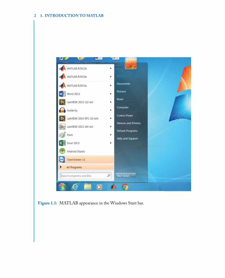
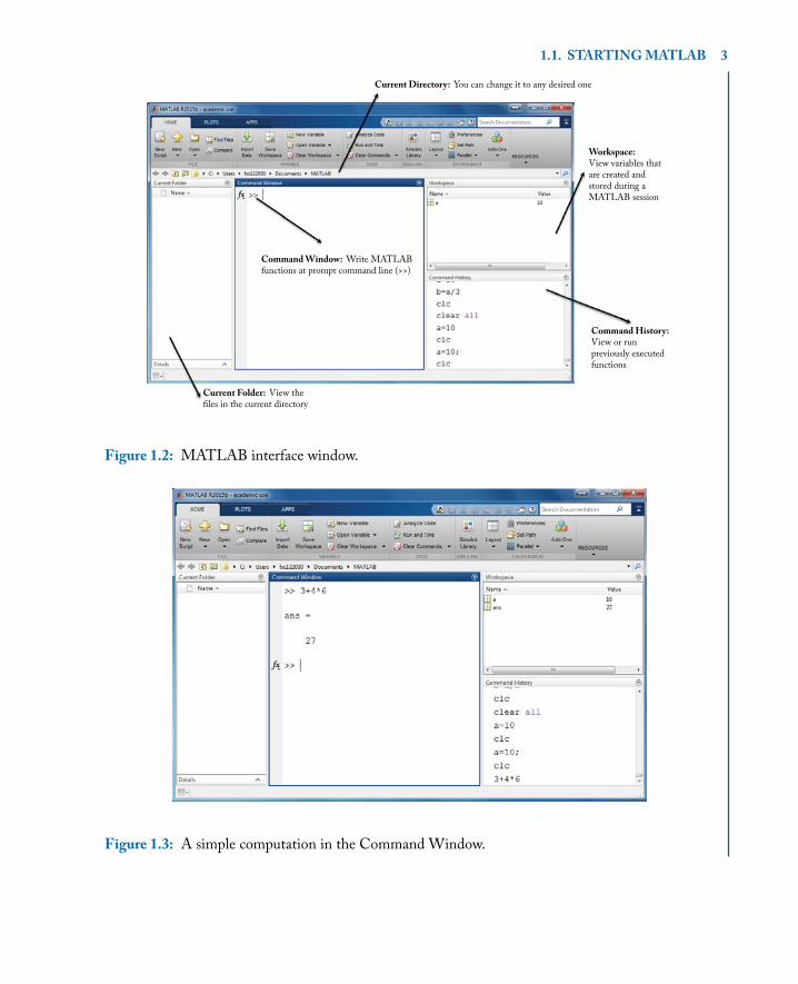
Assuming MATLAB is installed on the laptop or computer used, select MATLAB from theStart bar of Windows, as illustrated in Figure 1.1. After starting MATLAB, a window calledMATLAB desktop appears, see Figure 1.2, which contains other subwindows or panels. epanel CommandWindow allows interactive computation to be conducted. Suppose it is desiredto compute 3 C 4 � 6. is is done by typing it at the prompt command denoted by >> , seeFigure 1.3. Since no output variable is specified for the result of 3 C 4 � 6, MATLAB returns thevalue in the variable ans , which is created by MATLAB. Note that ans is always overwrittenby MATLAB, so, if the result is used for another operation, it needs to be assigned to a variable,for example x D 3 C 4 � 6.

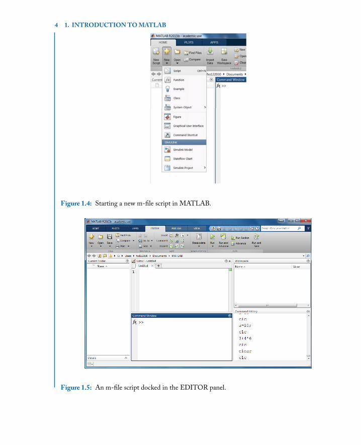
In practice, a sequence of operations is usually performed to achieve a desired output. Of-ten, a so-called m-file script is used for this purpose. An m-file script is a simple text file whereMATLAB commands are listed. Figure 1.4 shows how to start a new script. In the HOMEmenu, locate the New Script tab or locate it under New ! Script, or Ctrl+N to create a blankscript under the panel EDITOR. When a new script is opened, it looks as shown in Figure 1.5.A script can be saved using a specified name in a desired location. An m-file script needs to besaved with “.m” extension. When such a file is run, MATLAB reads the commands and executesthem as though there were typed sequentially. e following section provides further details onthe MATLAB commands and operations.

1.1.1 ARITHMETICOPERATIONSere are four basic arithmetic operators in m-files:

2 1. INTRODUCTIONTOMATLAB

Figure 1.1: MATLAB appearance in the Windows Start bar.

1.1. STARTINGMATLAB 3

Command History: View or run previously executed functions

Command Window: Write MATLABfunctions at prompt command line (>>)

Current Folder: View the!les in the current directory

Current Directory: You can change it to any desired one

Workspace:View variables thatare created and stored during aMATLAB session

Figure 1.2: MATLAB interface window.

Figure 1.3: A simple computation in the Command Window.


Figure 1.4: Starting a new m-file script in MATLAB.

Figure 1.5: An m-file script docked in the EDITOR panel.


..

+ addition- subtraction* multiplication/ division (for matrices, it also means inversion)

e following three operators work on an element-by-element basis:

..

.* multiplication of two vectors, element-wise

./ division of two vectors, element-wise

.^ raising all the elements of a vector to a power

As an example, to evaluate the expression a3 Cp

bd � 4c, where a D 1:2, b D 2:3, c D

4:5, and d D 4, type the following commands in the Command Window to get the answer( ans ):

..

>> a=1.2;>> b=2.3;>> c=4.5;>> d=4;>> a^3+sqrt(b*d)-4*cans =-13.2388

Note the semicolon after each variable assignment. If the semicolon is omitted, the inter-preter echoes back the variable value.

1.1.2 VECTOROPERATIONSConsider the vectors x D Œx1; x2; :::; xn� and y D Œy1; y2; :::; yn�. e following operations indi-cate the resulting vectors:

x: � y D Œx1y1; x2y2; :::; xnyn�

x:=y D Œx1

y1

;x2

y2

; :::;xn

yn

�

x: ^ p D Œx1p; x2

p; :::; xnp�:

Considering that the boldfacing of vectors/matrices are not used in .m files, in the notationadopted in this book, no boldfacing of vectors/matrices is shown to retain notation consistencywith .m files.


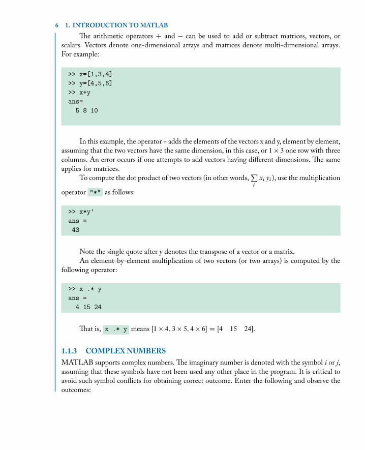
e arithmetic operators C and � can be used to add or subtract matrices, vectors, orscalars. Vectors denote one-dimensional arrays and matrices denote multi-dimensional arrays.For example:

..

>> x=[1,3,4]>> y=[4,5,6]>> x+yans=5 8 10

In this example, the operator + adds the elements of the vectors x and y, element by element,assuming that the two vectors have the same dimension, in this case, or 1 � 3 one row with threecolumns. An error occurs if one attempts to add vectors having different dimensions. e sameapplies for matrices.

To compute the dot product of two vectors (in other words,Pi

xiyi ), use the multiplication

operator "*" as follows:

..

>> x*y'ans =43

Note the single quote after y denotes the transpose of a vector or a matrix.An element-by-element multiplication of two vectors (or two arrays) is computed by the

following operator:

..

>> x .* yans =4 15 24

at is, x .* y means Œ1 � 4; 3 � 5; 4 � 6� D Œ4 15 24�.

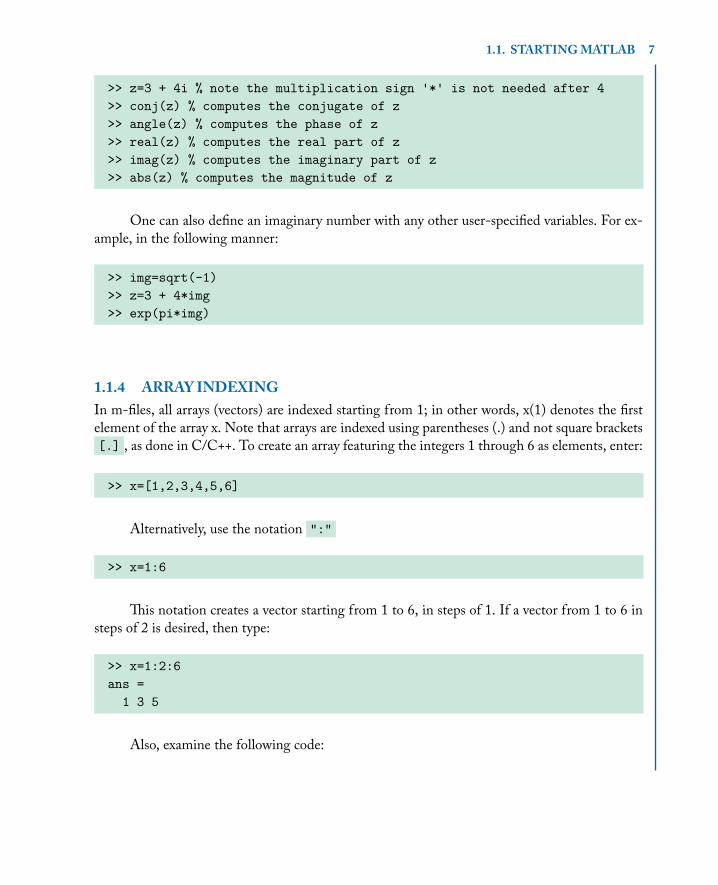
1.1.3 COMPLEXNUMBERSMATLAB supports complex numbers. e imaginary number is denoted with the symbol i or j,assuming that these symbols have not been used any other place in the program. It is critical toavoid such symbol conflicts for obtaining correct outcome. Enter the following and observe theoutcomes:


..

>> z=3 + 4i % note the multiplication sign '*' is not needed after 4>> conj(z) % computes the conjugate of z>> angle(z) % computes the phase of z>> real(z) % computes the real part of z>> imag(z) % computes the imaginary part of z>> abs(z) % computes the magnitude of z

One can also define an imaginary number with any other user-specified variables. For ex-ample, in the following manner:

..

>> img=sqrt(-1)>> z=3 + 4*img>> exp(pi*img)

1.1.4 ARRAY INDEXINGIn m-files, all arrays (vectors) are indexed starting from 1; in other words, x(1) denotes the firstelement of the array x. Note that arrays are indexed using parentheses (.) and not square brackets[.] , as done in C/C++. To create an array featuring the integers 1 through 6 as elements, enter:

.. >> x=[1,2,3,4,5,6]

Alternatively, use the notation ":"

.. >> x=1:6

is notation creates a vector starting from 1 to 6, in steps of 1. If a vector from 1 to 6 insteps of 2 is desired, then type:

..

>> x=1:2:6ans =1 3 5

Also, examine the following code:


..

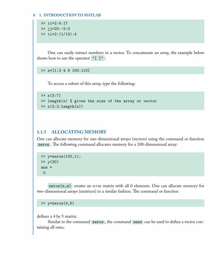
>> ii=2:4:17>> jj=20:-2:0>> ii=2:(1/10):4

One can easily extract numbers in a vector. To concatenate an array, the example belowshows how to use the operator "[ ]" :

.. >> x=[1:3 4 6 100:110]

To access a subset of this array, type the following:

..

>> x(3:7)>> length(x) % gives the size of the array or vector>> x(2:2:length(x))

1.1.5 ALLOCATINGMEMORYOne can allocate memory for one-dimensional arrays (vectors) using the command or functionzeros . e following command allocates memory for a 100-dimensional array:

..

>> y=zeros(100,1);>> y(30)ans =0

zeros(n,m) creates an n�m matrix with all 0 elements. One can allocate memory fortwo-dimensional arrays (matrices) in a similar fashion. e command or function

.. >> y=zeros(4,5)

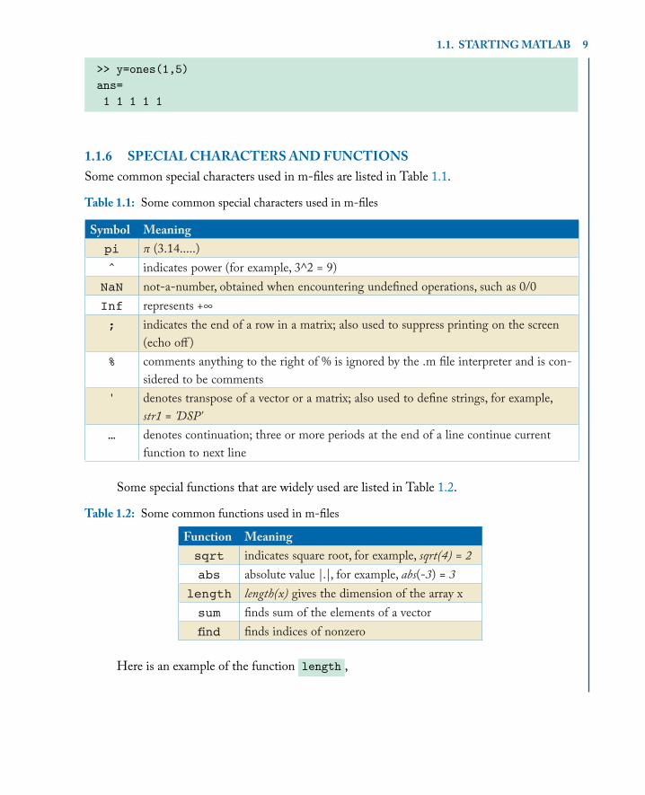
defines a 4 by 5 matrix.Similar to the command zeros , the command ones can be used to define a vector con-

taining all ones,


..

>> y=ones(1,5)ans=1 1 1 1 1

1.1.6 SPECIALCHARACTERSANDFUNCTIONSSome common special characters used in m-files are listed in Table 1.1.

Table 1.1: Some common special characters used in m-files

Symbol Meaning

pi π (3.14.....)

^ indicates power (for example, 3^2 = 9)

NaN not-a-number, obtained when encountering unde! ned operations, such as 0/0

Inf represents +∞

; indicates the end of a row in a matrix; also used to suppress printing on the screen

(echo o" )

% comments anything to the right of % is ignored by the .m ! le interpreter and is con-

sidered to be comments

' denotes transpose of a vector or a matrix; also used to de! ne strings, for example,

str1 = 'DSP'

… denotes continuation; three or more periods at the end of a line continue current

function to next line

Some special functions that are widely used are listed in Table 1.2.

Table 1.2: Some common functions used in m-files

Function Meaning

sqrt indicates square root, for example, sqrt(4) = 2

abs absolute value |.|, for example, abs(-3) = 3

length length(x) gives the dimension of the array x

sum ! nds sum of the elements of a vector

fi nd ! nds indices of nonzero

Here is an example of the function length ,


..

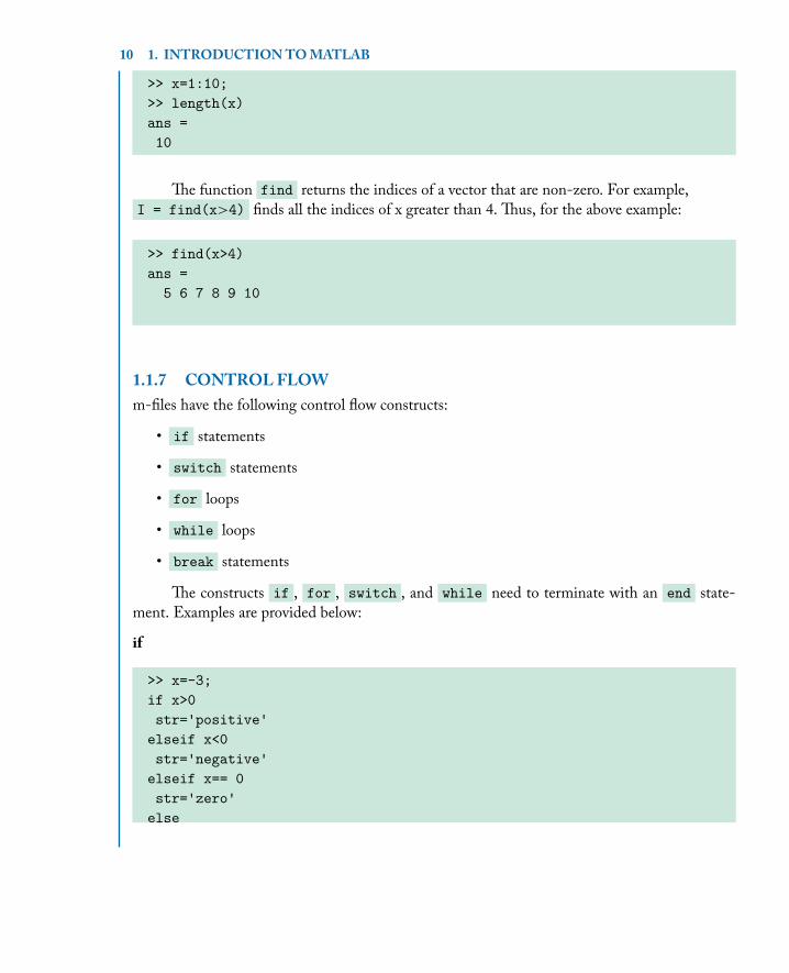
>> x=1:10;>> length(x)ans =10

e function find returns the indices of a vector that are non-zero. For example,I = find(x>4) finds all the indices of x greater than 4. us, for the above example:

..

>> find(x>4)ans =5 6 7 8 9 10

1.1.7 CONTROLFLOWm-files have the following control flow constructs:

• if statements

• switch statements

• for loops

• while loops

• break statements

e constructs if , for , switch , and while need to terminate with an end state-ment. Examples are provided below:

if

..

>> x=-3;if x>0str='positive'elseif x<0str='negative'elseif x== 0str='zero'else


..

str='error'end

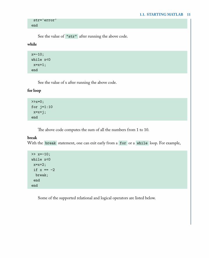
See the value of "str" after running the above code.

while

..

x=-10;while x<0x=x+1;end

See the value of x after running the above code.

for loop

..

>>x=0;for j=1:10x=x+j;end

e above code computes the sum of all the numbers from 1 to 10.

breakWith the break statement, one can exit early from a for or a while loop. For example,

..

>> x=-10;while x<0x=x+2;if x == -2break;endend

Some of the supported relational and logical operators are listed below.


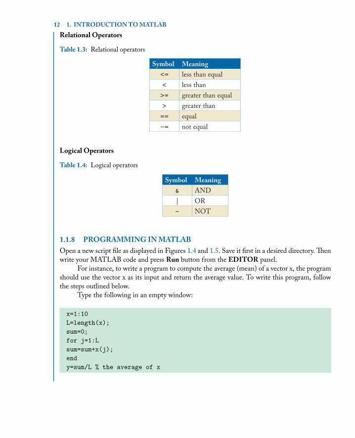
Relational Operators

Table 1.3: Relational operators

Symbol Meaning

<= less than equal

< less than

>= greater than equal

> greater than

== equal

~= not equal

Logical Operators

Table 1.4: Logical operators

Symbol Meaning

& AND

| OR

~ NOT

1.1.8 PROGRAMMING INMATLABOpen a new script file as displayed in Figures 1.4 and 1.5. Save it first in a desired directory. enwrite your MATLAB code and press Run button from the EDITOR panel.

For instance, to write a program to compute the average (mean) of a vector x, the programshould use the vector x as its input and return the average value. To write this program, followthe steps outlined below.

Type the following in an empty window:

..

x=1:10L=length(x);sum=0;for j=1:Lsum=sum+x(j);endy=sum/L % the average of x


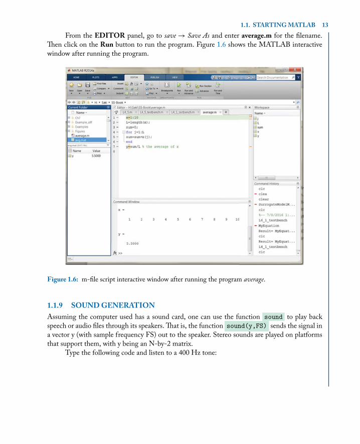
From the EDITOR panel, go to save ! Save As and enter average.m for the filename.en click on the Run button to run the program. Figure 1.6 shows the MATLAB interactivewindow after running the program.

Figure 1.6: m-file script interactive window after running the program average.

1.1.9 SOUNDGENERATIONAssuming the computer used has a sound card, one can use the function sound to play backspeech or audio files through its speakers. at is, the function sound(y,FS) sends the signal ina vector y (with sample frequency FS) out to the speaker. Stereo sounds are played on platformsthat support them, with y being an N-by-2 matrix.

Type the following code and listen to a 400 Hz tone:


..

>> t=0:1/8000:1;>> x=cos(2*pi*400*t);>> sound(x,8000);

Now generate a noise signal by typing:

..

>> noise=randn(1,8000); % generate 8000 samples of noise>> sound(noise,8000);

e function randn generates Gaussian noise with zero mean and unit variance.

1.1.10 LOADINGANDSAVINGDATAOne can load or store data using the commands load and save . To save the vector x of theabove code in the file data.mat, type:

.. >> save('data.mat', 'x')

To retrieve the data saved, type:

.. >> load data

e vector x gets loaded in memory. To see memory contents, use the command whos ,

..

>> whosVariable Dimension Typex 1x8000 double array

e command whos gives a list of all the variables currently in memory, along with theirdimensions and data type. In the above example, x contains 8,000 samples.

To clear up memory after loading a file, type clear all when done. is is importantbecause, if one does not clear all the variables, conflicts can occur with other codes using the samevariables.

1.1.11 READINGWAVEAND IMAGEFILESWith MATLAB, one can read data from different file types (such as .wav, .jpeg, and .bmp) andload them in a vector.

1.2. MATLABPROGRAMMINGEXAMPLES 15

To read an audio data file with .wav extension, use the following command:

.. >> [y,Fs]=audioread('filename')

is command reads a wave file specified by the string filename and returns the sampleddata in y with the sampling rate of Fs (in hertz).

To read an image file, use the following command:

.. >> [y]=imread('filename')

is command reads a grayscale or color image from the string filename and returns theimage data in the array y.

1.1.12 SIGNALDISPLAYGraphical tools are available in MATLAB to display data in a graphical form. roughout thebook, signals in both the time and frequency domains are displayed using the function plot,

.. >> plot(x,y)

is function creates a 2-D line plot of the data in y versus corresponding x values.

1.2 MATLABPROGRAMMINGEXAMPLESIn this section, several simple MATLAB programs are presented.

1.2.1 SIGNALGENERATIONIn this example, we see how to generate and display continuous-time signals in the time domain.One can represent such signals as a function of time. For simulation purposes, a representation oftime t is needed. Note that the time scale is continuous while computers handle operations in adiscrete manner. Continuous time simulation is achieved by considering a very small time inter-val. For example, if a 1-second duration signal in millisecond (msec) increments (time interval of0.001 second) is considered, then one sample every 1 msec or a total of 1,000 samples are gener-ated for the entire signal, leading to a continuous signal simulation. is continuous-time signalapproximation or simulation is used in later chapters. It is important to note that a finite numberof samples is involved in the simulation of a continuous-time signal, and thus to differentiate acontinuous-time signal from a discrete-time signal, a much higher number of samples per secondfor a continuous-time signal needs to be used (very small time interval).


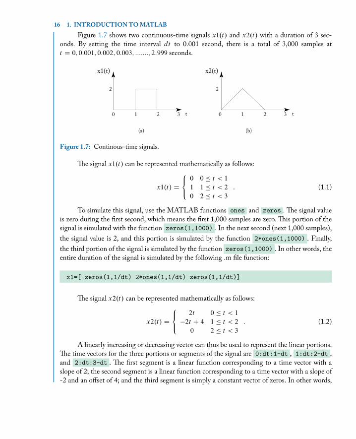
Figure 1.7 shows two continuous-time signals x1.t/ and x2.t/ with a duration of 3 sec-onds. By setting the time interval dt to 0.001 second, there is a total of 3,000 samples att D 0; 0:001; 0:002; 0:003; :::::::; 2:999 seconds.

x1(t)

2

0 1 2 3 t

(a)

x2(t)

2

0 1 2 3 t

(b)

Figure 1.7: Continous-time signals.

e signal x1.t/ can be represented mathematically as follows:

x1.t/ D

8<: 0 0 � t < 1

1 1 � t < 2

0 2 � t < 3

: (1.1)

To simulate this signal, use the MATLAB functions ones and zeros . e signal valueis zero during the first second, which means the first 1,000 samples are zero. is portion of thesignal is simulated with the function zeros(1,1000) . In the next second (next 1,000 samples),the signal value is 2, and this portion is simulated by the function 2*ones(1,1000) . Finally,the third portion of the signal is simulated by the function zeros(1,1000) . In other words, theentire duration of the signal is simulated by the following .m file function:

.. x1=[ zeros(1,1/dt) 2*ones(1,1/dt) zeros(1,1/dt)]

e signal x2.t/ can be represented mathematically as follows:

x2.t/ D

8<: 2t 0 � t < 1

�2t C 4 1 � t < 2

0 2 � t < 3

: (1.2)

A linearly increasing or decreasing vector can thus be used to represent the linear portions.e time vectors for the three portions or segments of the signal are 0:dt:1-dt , 1:dt:2-dt ,and 2:dt:3-dt . e first segment is a linear function corresponding to a time vector with aslope of 2; the second segment is a linear function corresponding to a time vector with a slope of-2 and an offset of 4; and the third segment is simply a constant vector of zeros. In other words,

1.2. MATLABPROGRAMMINGEXAMPLES 17

the entire duration of the signal for any value of dt can be simulated by the following .m filefunction:

.. x2=[2*(0:dt:(1-dt))-2*(1:dt:(2-dt))+4 zeros(1,1/dt)]

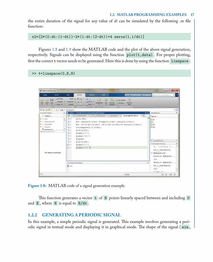
Figures 1.8 and 1.9 show the MATLAB code and the plot of the above signal generation,respectively. Signals can be displayed using the function plot(t,data) . For proper plotting,first the correct t vector needs to be generated.Here this is done by using the function linspace :

.. >> t=linspace(0,E,N)

Figure 1.8: MATLAB code of a signal generation example.

is function generates a vector t of N points linearly spaced between and including 0and E , where N is equal to E/dt .

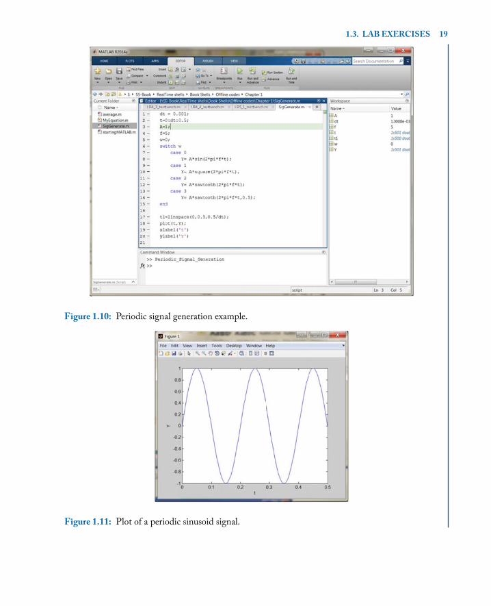
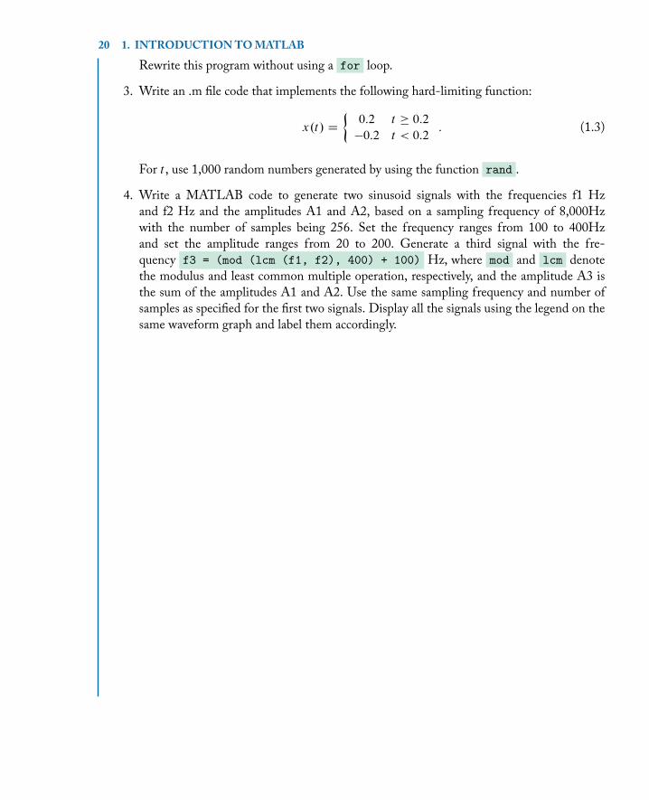
1.2.2 GENERATINGAPERIODIC SIGNALIn this example, a simple periodic signal is generated. is example involves generating a peri-odic signal in textual mode and displaying it in graphical mode. e shape of the signal ( sin ,


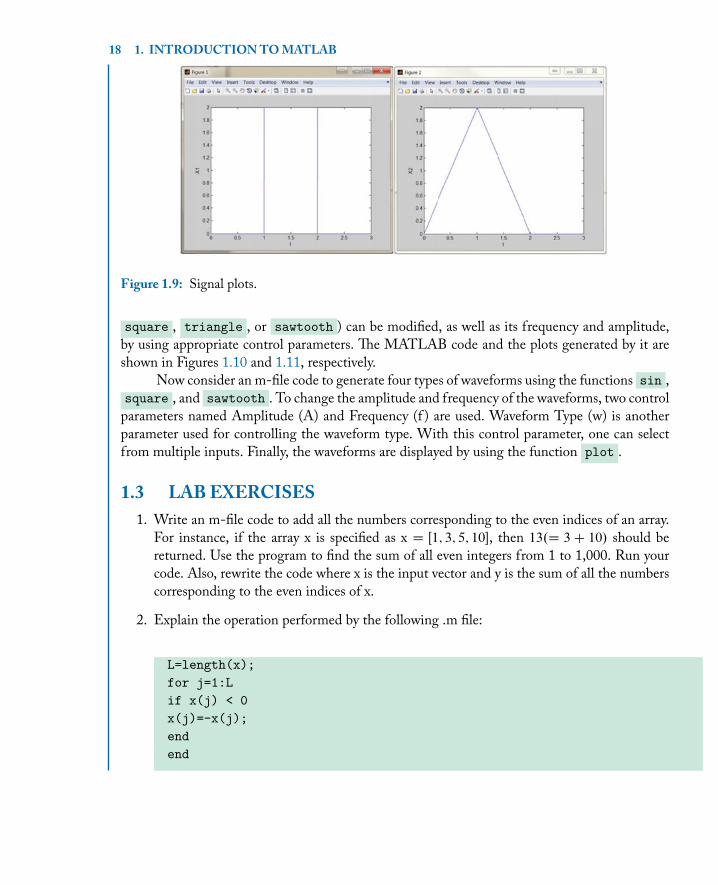
Figure 1.9: Signal plots.

square , triangle , or sawtooth ) can be modified, as well as its frequency and amplitude,by using appropriate control parameters. e MATLAB code and the plots generated by it areshown in Figures 1.10 and 1.11, respectively.

Now consider an m-file code to generate four types of waveforms using the functions sin ,square , and sawtooth . To change the amplitude and frequency of the waveforms, two controlparameters named Amplitude (A) and Frequency (f ) are used. Waveform Type (w) is anotherparameter used for controlling the waveform type. With this control parameter, one can selectfrom multiple inputs. Finally, the waveforms are displayed by using the function plot .

1.3 LABEXERCISES1. Write an m-file code to add all the numbers corresponding to the even indices of an array.

For instance, if the array x is specified as x D Œ1; 3; 5; 10�, then 13.D 3 C 10/ should bereturned. Use the program to find the sum of all even integers from 1 to 1,000. Run yourcode. Also, rewrite the code where x is the input vector and y is the sum of all the numberscorresponding to the even indices of x.

2. Explain the operation performed by the following .m file:

..

L=length(x);for j=1:Lif x(j) < 0x(j)=-x(j);endend

1.3. LABEXERCISES 19

Figure 1.10: Periodic signal generation example.

Figure 1.11: Plot of a periodic sinusoid signal.


Rewrite this program without using a for loop.

3. Write an .m file code that implements the following hard-limiting function:

x.t/ D

�0:2 t � 0:2

�0:2 t < 0:2: (1.3)

For t , use 1,000 random numbers generated by using the function rand .

4. Write a MATLAB code to generate two sinusoid signals with the frequencies f1 Hzand f2 Hz and the amplitudes A1 and A2, based on a sampling frequency of 8,000Hzwith the number of samples being 256. Set the frequency ranges from 100 to 400Hzand set the amplitude ranges from 20 to 200. Generate a third signal with the fre-quency f3 = (mod (lcm (f1, f2), 400) + 100) Hz, where mod and lcm denotethe modulus and least common multiple operation, respectively, and the amplitude A3 isthe sum of the amplitudes A1 and A2. Use the same sampling frequency and number ofsamples as specified for the first two signals. Display all the signals using the legend on thesame waveform graph and label them accordingly.

anywhere-anytime signalsandsystemslaboratory · anywhere-anytime signalsandsystemslaboratory...

Documents