“Advances in Continuous Replenishment Systems”

Edmund W. Schuster

Massachusetts Institute of Technology

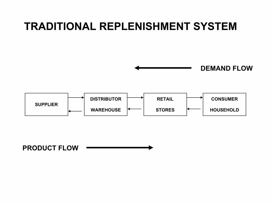
TRADITIONAL REPLENISHMENT SYSTEM

DEMAND FLOW

DISTRIBUTOR

WAREHOUSE

RETAIL

STORES

CONSUMER

HOUSEHOLDSUPPLIER

PRODUCT FLOW

THE FUTURE

PAPERLESS INFORMATION FLOW

DISTRIBUTOR

WAREHOUSE

RETAIL

STORES

CONSUMER

HOUSEHOLDSUPPLIER

PRODUCT FLOW MATCHED TO CONSUMPTION

Continuous Replenishment Systems

• One cycle re-point point • Some systems use DRP methodology• Dynamic re-order point• Simple logic• Require “extra” work

Forecasting Customer Demand

• Use live data on customer withdrawals• Focused forecasting (best fit from moving

average, exponential smoothing, Holt’s method and history)

• Time series methods lag the trend• forecast bias causes a problem• See Krupp, J.A.G., 1982, “Effective Safety

Stock Planning,” P&IM, Third Quarter.

Advanced Forecasting Methods

• Box-Jenkins

• Complexity of model must be justified

• Neural networks enhance time series methods

• L.L. Bean (see Andrews and Cunningham, 1995)

HIERARCHY OF PRODUCTION DECISIONS

Forecasts of future demand

Aggregate plan

Master production schedule

Schedule of production quantities by product and time period

Materials requirements planning system

Explode master schedule to obtain requirements for components and final product

Detailed job shop schedule

To meet specification of production quantities from MRP system

FIGURE 1

The Supply Chain Model

Forecast

Continuous Replenishment System (CRP)

Truck Loading System

Finite Production Planning System

Material Requirements Planning (MRP)

Corp.Logistics

PlantSystems

Supplier Vendor

Supply Chain Dynamics

• Production planning and scheduling• Lot sizing• MRP• Continuous Replenishment Systems• System Dynamics (the “beer game” and

MIT)• “Fits and Starts”

The Supply Chain Model

• Characterized by dynamic inventory swings• Inventory swings often dramatic• “System Dynamics” (see Sterman, 1992)• Minimize deviations in the supply chain• A mix of models may prove the best

solution to this problem (see Cleaves and Masch, 1996)

R.P. Without Safety Stock

(u)(t)

R.P.P

Inv.Level

t Time

R.P. With Safety Stock

Time

Inv.Level

P

SS

The Truck Loading Problem

• Provide an even run-out of all sku’s in a customers warehouse

• Reduce air weight• Enhance plant warehouse efficiency

Step 1. When a single SKU at a customer warehouse drops below its re-order point, start procedure.

Step 2. For each SKU in the customers warehouse, net existing inventory from the daily demand forecast.

Step 3. After netting out inventory, convert into weight per day for each SKU.

Step 4. Sum the weight per day for all SKU’s to get a total weight per day

Step 5. Calculate the cumulative weight per day. When cumulative weight per day is just shy of a full truck load, stop

Decision Variable:

x(i) = number of layers of product i

Constants:

w(i) = weight per layer for SKU i (pounds/layer)

c(i) = total weight of SKU corresponding to run-out calculated in step 5 (pounds)

t = total weight of order (pounds)

An Example From Welch’s CRP System

Step 1 - Assuming a SKU has dropped below its re-order point, we move to step 2

Step 2 - Table 1 shows beginning inventory netted against forecast

Step 3 - Table 2 converts case forecast (Table 1) into weight per SKU, per day

Step 4 - At the bottom of Table 2, we sum the weight per day for all products

TABLE 1 - Forecast Netted for Inventory (all values in cases)

Product Code Day 1 Day 2 Day 3 Day 4 Day 5 Day 6 Day 7 Day 8 Day 9 Day 10 Day 11 Day 12 Day 13

4180021100 0 0 0 0 0 0 0 0 0 0 15 15 154180022800 0 0 0 0 7 7 7 6 6 6 6 6 64180022900 0 0 0 0 0 0 0 0 0 0 0 18 184180050200 0 0 0 0 0 0 0 0 0 0 0 0 54180050300 0 0 0 0 0 0 0 7 7 7 7 7 74180050500 0 0 0 0 0 0 0 0 0 0 0 6 64180050701 0 0 0 0 0 0 0 0 0 0 3 3 34180055200 0 0 0 0 0 0 0 0 0 0 0 14 144180055300 0 0 0 0 0 0 0 0 0 0 0 3 34180056300 0 0 0 0 0 0 0 0 0 0 0 4 44180070500 0 0 0 0 0 0 0 0 0 0 0 14 144180010300 0 0 0 0 0 0 21 20 20 20 20 20 204180010900 0 0 0 0 0 0 0 0 32 32 32 32 324180011500 0 0 0 0 0 0 60 54 54 54 54 54 544180011600 0 0 0 0 0 0 0 40 40 40 40 40 404180011700 0 0 0 0 0 0 0 52 52 52 52 52 524180011900 0 0 0 0 0 0 0 0 65 65 65 65 654180012800 0 0 0 0 0 0 0 0 17 17 17 17 174180013300 0 0 0 0 0 0 0 0 0 0 54 54 544180013500 0 0 0 0 0 0 0 0 0 61 61 61 614180013600 0 0 0 0 0 0 0 0 52 52 52 52 524180014000 0 0 0 0 0 0 0 47 47 47 47 47 474180014500 0 0 0 0 0 0 0 0 20 20 20 20 204180015000 0 0 0 0 0 0 0 0 19 19 19 19 194180015100 0 0 0 0 0 0 0 0 0 0 0 9 94180018100 0 0 0 0 0 0 0 15 15 15 15 15 154180018200 0 0 0 0 0 0 0 17 17 17 17 17 17

TABLE 2 - Accumulated Weight Per Day (all values in pounds) Cumulated WeightPer Product

Product Code Day 1 Day 2 Day 3 Day 4 Day 5 Day 6 Day 7 Day 8 Day 9 Day 10 Day 11 Day 12 Day 13 (12 Days)

4180021100 0 0 0 0 0 0 0 0 0 0 593 593 593 11854180022800 0 0 0 0 330 330 330 243 243 243 243 243 243 22044180022900 0 0 0 0 0 0 0 0 0 0 0 708 708 7084180050200 0 0 0 0 0 0 0 0 0 0 0 0 157 04180050300 0 0 0 0 0 0 0 88 88 88 88 88 88 4424180050500 0 0 0 0 0 0 0 0 0 0 0 128 128 1284180050701 0 0 0 0 0 0 0 0 0 0 61 61 61 1214180055200 0 0 0 0 0 0 0 0 0 0 0 468 468 4684180055300 0 0 0 0 0 0 0 0 0 0 0 42 42 424180056300 0 0 0 0 0 0 0 0 0 0 0 46 46 464180070500 0 0 0 0 0 0 0 0 0 0 0 531 531 5314180010300 0 0 0 0 0 0 526 489 489 489 489 489 489 29704180010900 0 0 0 0 0 0 0 0 417 417 417 417 417 16664180011500 0 0 0 0 0 0 751 675 675 675 675 675 675 41244180011600 0 0 0 0 0 0 0 521 521 521 521 521 521 26034180011700 0 0 0 0 0 0 0 650 650 650 650 650 650 32514180011900 0 0 0 0 0 0 0 0 817 817 817 817 817 32704180012800 0 0 0 0 0 0 0 0 215 215 215 215 215 8614180013300 0 0 0 0 0 0 0 0 0 0 676 676 676 13524180013500 0 0 0 0 0 0 0 0 0 757 757 757 757 22714180013600 0 0 0 0 0 0 0 0 645 645 645 645 645 25824180014000 0 0 0 0 0 0 0 585 585 585 585 585 585 29254180014500 0 0 0 0 0 0 0 0 503 503 503 503 503 20134180015000 0 0 0 0 0 0 0 0 208 208 208 208 208 8324180015100 0 0 0 0 0 0 0 0 0 0 0 99 99 994180018100 0 0 0 0 0 0 0 198 198 198 198 198 198 9884180018200 0 0 0 0 0 0 0 222 222 222 222 222 222 1112

Total Wt./Day 0 0 0 0 330 330 1607 3670 6476 7233 8562 10584 10741 38793

Cumulated 0 0 0 0 330 660 2267 5937 12413 19647 28209 38793 49534

Step 5 - As the cumulative weight per day approaches 44,500 pounds we stop. In the example this occurs at day 12. At this stage, all products have an equal run out, but we are just shy of filling the truck (at day 12, cumulative weight equals 38,793 pounds, at day 13 the cumulativeweight is 49,534). We also do not have each product rounded to even case layers.

Step 6 - The total weight for each SKU found in step 5 becomes c(i). Bysolving the IP, we find the number of layers for each item that results in a truck weight as close to 44,500 pounds as possible.

The solution equals 44,483 pounds.

Improvements to CRP Software

• Time phased future orders (DRP)• Better methods to plan safety stock• Insure even run-outs for each sku in a

customers warehouse• Truck loading methods