ap biology lab-02

1Copyright © 2013 Quality Science Labs, LLC

Lab 2Hardy-Weinberg Equilibrium: Modeling

Allele Frequencies in Populations

Big Idea 1: EvolutionHow can mathematical models be used to investigate the relationship between allele

frequencies in populations of organisms and evolutionary changes within populations?

Please be sure you have read thestudent intro packet before you do this lab.

(If needed, the student intro packet is available at www.qualitysciencelabs.com/AdvancedBioIntro.pdf)

Lab Investigations SummaryPre-lab and Questions: Estimating Allele Frequencies

Estimating allele frequencies for a specific trait – PTC taste test – within a sample population using Hardy-Weinberg equilibrium.; analysis of global variation in sensitivity to bitter tasting PTC

Lab Investigation 2.1: A Micro-Evolution SimulationA micro-evolution simulation of eastern gray squirrels to demonstrate Hardy-Weinberg equilibrium, natural selection, and genetic driftScenario #1 Hardy-Weinberg EquilibriumScenario #2 Natural SelectionScenario #3 Genetic Drift

Lab Investigation 2.2: Mathematical ModelingPart 1 - Tutorial

Using mathematical models of Hardy-Weinberg equilibrium to predict population changes; tutorial on Hardy-Weinberg spreadsheet modeling

Part 2 - Student Guided InquirySeven steps to model building in biology using the Hardy-Weinberg spreadsheet modeling

2 Copyright © 2013 Quality Science Labs, LLC

Lab 2 - Hardy-Weinberg Equilibrium: Modeling Allele Frequencies in Populations

Big Idea 1: Evolution

How can mathematical models be used to investigate the relationship between allele frequencies in populations of organisms and evolutionary changes within populations? (Note: A population is the total of all the organisms of the same group or species, who live in the same geographical area, and have the capability of interbreeding.)

BACKGROUND

•Evolution is a general term with many diverse meanings. Evolution in a general sense means change over time. Evolution can refer to universal evolution, planetary evolution, chemical evolution, biological evolution, macro and micro evolution. We are focused on biological evolution in this course.

•The biological sciences define evolution as the sum total of the genetically inherited changes in the individuals who are the members of a population’s gene pool. It is clear that the effects of evolution are felt by individuals, but it is the population as a whole that actually changes over time. Evolution is simply a change in frequencies of alleles in the gene pool of a population. For instance, let us assume that there is a trait that is determined by the inheritance of a gene with two alleles — B and b. If the parent generation has 92% B and 8% b and their offspring have 90% B and 10% b, a slight change has occurred between the generations. The population’s gene pool has changed in the direction of a higher frequency of the b allele — it was not just those individuals who inherited the b allele who evolved.

•The term evolution can have different interpretations and must be defined when used. There are two distinct types of evolution that should be clarified when using the term. Evolution can refer to changes within similar breeding organisms or in other words, the capacity of an existing genotype to vary within limits. Evolution can also refer to the origin of new genetic information resulting in changes from one kind of organism to another over time. It is the challenge of this kind of evolution, however, to account for the origin of new genetic information.

•As scientists, we are focusing on the actual changes that can be observed today within populations, species, or taxonomic groups. Some may be caused by mechanisms such as natural selection, genetic drift, migrations, and mutations (although most mutations are harmful and do not stay in the gene pool.) These observable changes include balancing selection (conservative) — maintenance of two or more genetic variants at frequencies higher than can be accounted for by random processes. A prime example is Sickle-cell anemia in malaria


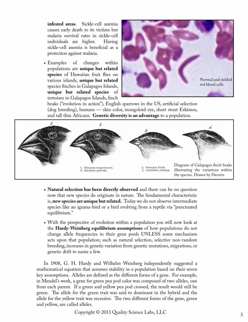
infested areas. Sickle-cell anemia causes early death to its victims but malaria survival rates in sickle-cell individuals are higher. Having sickle-cell anemia is beneficial as a protection against malaria.

•Examples of changes within populations are unique but related species of Hawaiian fruit flies on various islands, unique but related species finches in Galapagos Islands, unique but related species of tortoises in Galapagos Islands, finch beaks (“evolution in action”), English sparrows in the US, artificial selection (dog breeding), humans — skin color, mongoloid eye, short stout Eskimos, and tall thin Africans. Genetic diversity is an advantage to a population.

•Natural selection has been directly observed and there can be no question now that new species do originate in nature. The fundamental characteristic is, new species are unique but related. Today we do not observe intermediate species like an iguana-bird or a bird evolving from a reptile via “punctuated equilibrium.”

•With the perspective of evolution within a population you will now look at the Hardy-Weinberg equilibrium assumptions of how populations do not change allele frequencies in their gene pools UNLESS some mechanism acts upon that population; such as natural selection, selective non-random breeding, increases in genetic variation from genetic mutations, migrations, or genetic drift to name a few.

In 1908, G. H. Hardy and Wilhelm Weinberg independently suggested a mathematical equation that assumes stability in a population based on their seven key assumptions. Alleles are defined as the different forms of a gene. For example, in Mendel’s work, a gene for green pea pod color was composed of two alleles, one from each parent. If a green and yellow pea pod crossed, the result would still be green. The allele for the green trait was said to dominant in the hybrid and the allele for the yellow trait was recessive. The two different forms of the gene, green and yellow, are called alleles.

Diagram of Galapagos finch beaks illustrating the variations within the species. Drawn by Darwin

Normal and sickled red blood cells


•The Hardy-Weinberg (H-W) equilibrium equation evaluates the occurrence or frequency of the two alleles. If one is A and the other is a, then the possibilities of paired alleles are AA, Aa, and aa. If in a population of 100, the frequency of A (p) is 40%, then the frequency of a (q) is 60% (A + a = 1.0 or p + q = 1.0). The frequency of the diploid combinations (AA, Aa, and aa) is expressed mathematically as p2 + 2pq + q2 = 1.0 where p2 is the homozygous dominant AA, pq is the heterozygous Aa, and q2 is the homozygous recessive aa.

•Hardy-Weinberg also set up the null hypothesis (there is no relationship between the independent and dependant variables) based on five key assumptions. If the five assumptions were met, and if the population’s allele and genotype frequencies did change from generation to generation, then the conclusion must be that evolution was involved in some way. This is a way to model evolutionary changes in a population of alleles. The five assumptions are:

1. The breeding population is large. 2. Mating is random. 3. There is no mutation of the alleles or alteration in the DNA

sequencing. 4. There is no immigration or emigration occurring. 5. There is no natural selection for survival and reproduction.

All genotypes have an equal chance.

•These conditions are the absence of the things that can cause evolution. In other words, if no mechanisms of change are acting on a population, the population will remain stable meaning, the gene pool frequencies will remain unchanged. However, changes in the population are likely to occur because it is highly likely that any or all of these seven conditions will happen in the real world.

•By comparing genotype frequencies from the next generation with those of the current generation in a population, one can also learn whether or not evolution has occurred and in what direction and rate for a selected trait. However, the Hardy-Weinberg equation cannot determine which of the various possible causes of change were responsible for the changes in gene pool frequencies.

•What is the significance of H-W? It is important not to lose sight of the fact that gene pool frequencies are inherently stable. They do not change by themselves. Despite the fact that evolution is a common occurrence within natural populations, allele frequencies will remain unaltered indefinitely unless evolutionary mechanisms such as mutation and natural selection cause them to change.

•Before Hardy and Weinberg, it was thought that dominant alleles must, over time, inevitably swamp recessive alleles out of existence. This incorrect theory was called genophagy (literally “gene eating”). According to this theory, dominant alleles always increase in frequency from generation to generation. Hardy and Weinberg were able to demonstrate with their equation that


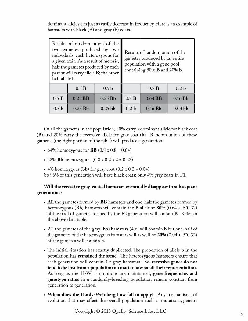
dominant alleles can just as easily decrease in frequency. Here is an example of hamsters with black (B) and gray (b) coats.

Of all the gametes in the population, 80% carry a dominant allele for black coat (B) and 20% carry the recessive allele for gray coat (b). Random union of these gametes (the right portion of the table) will produce a generation:

•64% homozygous for BB (0.8 x 0.8 = 0.64)

•32% Bb heterozygotes (0.8 x 0.2 x 2 = 0.32)

•4% homozygous (bb) for gray coat (0.2 x 0.2 = 0.04)So 96% of this generation will have black coats; only 4% gray coats in F1.

Will the recessive gray-coated hamsters eventually disappear in subsequent generations?

•All the gametes formed by BB hamsters and one-half the gametes formed by heterozygous (Bb) hamsters will contain the B allele so 80% (0.64 + .5*0.32) of the pool of gametes formed by the F2 generation will contain B. Refer to the above data table.

•All the gametes of the gray (bb) hamsters (4%) will contain b but one-half of the gametes of the heterozygous hamsters will as well, so 20% (0.04 + .5*0.32) of the gametes will contain b.

•The initial situation has exactly duplicated. The proportion of allele b in the population has remained the same. The heterozygous hamsters ensure that each generation will contain 4% gray hamsters. So, recessive genes do not tend to be lost from a population no matter how small their representation. As long as the H-W assumptions are maintained, gene frequencies and genotype ratios in a randomly-breeding population remain constant from generation to generation.

•When does the Hardy-Weinberg Law fail to apply? Any mechanisms of evolution that may affect the overall population such as mutations, genetic

Results of random union of the two gametes produced by two individuals, each heterozygous for a given trait. As a result of meiosis, half the gametes produced by each parent will carry allele B; the other half allele b.

Results of random union of the gametes produced by an entire population with a gene pool containing 80% B and 20% b.

0.5 B 0.5 b 0.8 B 0.2 b

0.5 B 0.25 BB 0.25 Bb 0.8 B 0.64 BB 0.16 Bb

0.5 b 0.25 Bb 0.25 bb 0.2 b 0.16 Bb 0.04 bb


drift, mating selectivity, natural selection, migrations or emigrations, small populations, or lack of randomness in mating will nullify the H-W equilibrium.

•How does Natural Selection affect allele frequencies in a population’s gene pool? In some cases, we can directly observe natural selection. Very convincing data show that the shape of finches’ beaks on the Galapagos Islands is connected to the weather patterns: after droughts, the finch population that survives has deeper, stronger beaks that let them eat tougher seeds. In other cases, human activity has led to environmental changes that have caused populations to evolve through natural selection. An example is that of the population of dark moths in the 19th century in England, which rose and fell in parallel to industrial pollution. These changes can often be observed and documented, although the study is incomplete and there may be other factors besides the moth colorations that contributed to the gene pool frequency changes (Majerus, 1999). Fitness and sexual selection are rated based on an organism's ability to survive and produce offspring. A genotype’s fitness depends on the environment in which the organism lives. The fittest individual is not necessarily the strongest, fastest, or biggest. A genotype’s fitness includes its ability to survive, find a mate, produce offspring and ultimately, leave its genes in the next generation.

•What is Genetic Drift and how can it alter allele frequencies in a population’s gene pool? Genetic drift is a mechanism of evolution that occurs by random chance rather than natural selection. In genetic drift, a population experiences a change in the frequency of a given allele, prompted by random luck rather than a need for adaptation. In each generation, some individuals may, just by chance, leave behind a few more descendants (and genes, of course) than other individuals. The genes of the next generation will be the genes of the “lucky” individuals, not necessarily the healthier or “better” individuals.

The Pre-lab is a chance to sample your own genetic makeup in the PTC taste test and to compare your sample to global population data. In Lab Investigation 2.1 you will simulate the H-W Equilibrium, Natural Selection, and Genetic Drift. The last investigation will utilize computer modeling to manipulate data from large and random populations to verify allele frequency changes in a population's gene pool using H-W equilibrium and natural selection scenarios.


PREPARATION

Materials and Equipment are listed with each lab separately.

Timing and Length of Lab Activities The Pre-lab Investigation can be done in one lab period. Lab Investigation 2.1

will take two lab periods to collect data from each lab group, graph the data, and hold discussions. Lab Investigation 2.2 is a tutorial on building a spreadsheet for H-W Equilibrium that students can use in the Part 2 - Student Guided Inquiry. Lab Investigation 2.2 will take two lab periods.

Learning objectives aligned to standards and science practices (SP)

•To convert a data set from a table of numbers that reflect a change in the genetic makeup of a population over time and to apply mathematical methods and conceptual understanding to investigate the cause and effect of this change (1A1 and SP 1.5, SP 2.2).

•To apply mathematical methods to data from a real or simulated population to predict what will happen to the population in the future (1A1 and SP 2.2).

•To evaluate data-based evidence that describes evolutionary changes in the allele frequencies of a population over time (1A1 and SP 5.3).

•To use data from mathematical models based on the Hardy-Weinberg equilibrium to analyze and justify genetic drift and the effects of selection in the evolution of specific populations (1A3 and SP 1.4, SP 2.1).

•To describe a model that represents evolution within a population (1C3 and SP 5.3).

•To evaluate given data sets that illustrate observable evolution as an ongoing process within populations (1C3 and SP 5.3).

General Safety Precautions are not a concern with these labs using beads and PTC taste test strips. Computer spreadsheet development precautions include periodically saving work.


Pre-lab and Questions:Estimating Allele Frequencies

Estimating Allele Frequencies for a Specific Trait – PTC Taste test – Within a Sample Population using Hardy-Weinberg Equilibrium

As described in the Background, the Hardy-Weinberg Equation is: p2 + 2pq + q2 = 1.0

This is where p2 represents both alleles dominate (TT), 2pq represents one allele dominate (T) and one recessive (t), and q2 represents both alleles recessive (tt).

Dr. Arthur Fox, a DuPont® chemist in 1931, accidently released a cloud of the dry chemical and a nearby colleague complained of its bitter taste. Dr. Fox, who was standing much closer, did not detect any of the bitterness. Dr. Fox then tested his family members and friends, laying the genetic groundwork for the PTC (phenylthiocarbamide) test. This test was actually used for paternity testing before the days of DNA.

Although PTC is not found in nature, the ability to taste it correlates strongly with the ability to taste other bitter substances that do occur naturally, many of which are alkaloid toxins. Today we know that the ability to taste PTC (or not) is conveyed by a single gene that codes for a taste receptor on the tongue. The PTC gene, TAS2R38, was discovered in 2003.

Use your class as a sample population. (If you are not in a class, test as many members of your family as possible, as well as friends). You will be using PTC test strips for bitter or no taste. The allele frequency of a gene controlling the ability to taste the chemical PTC will be estimated in your sample population. A strong bitter-taste reaction to PTC is evidence of the presence of a dominant allele (it could be either homozygous (TT) or heterozygous (Tt). No taste can only be the homozygous (tt) recessive alleles.

Later researchers (Bartoshuk et al.1994) observed that not all tasters were alike. Some tasters reacted more strongly and characterized PTC as very bitter. It was hypothesized that the homozygous dominant TT genotype characterized supertasters and the heterozygous Tt correlated with medium tasters.

To estimate the frequency of the PTC-tasting allele in your sample population, first find the value of q by taking the square root of q2 (tt alleles). Then find p = 1-q. (Why not p first?)

Other interesting facts about PTC:

•People who can taste PTC are more likely to be non-smokers and to not be in the habit of drinking coffee or tea.

•People who are super-tasters are more likely to find green vegetables bitter.

•Women, Asians, and African-Americans are all more likely to be super-tasters.


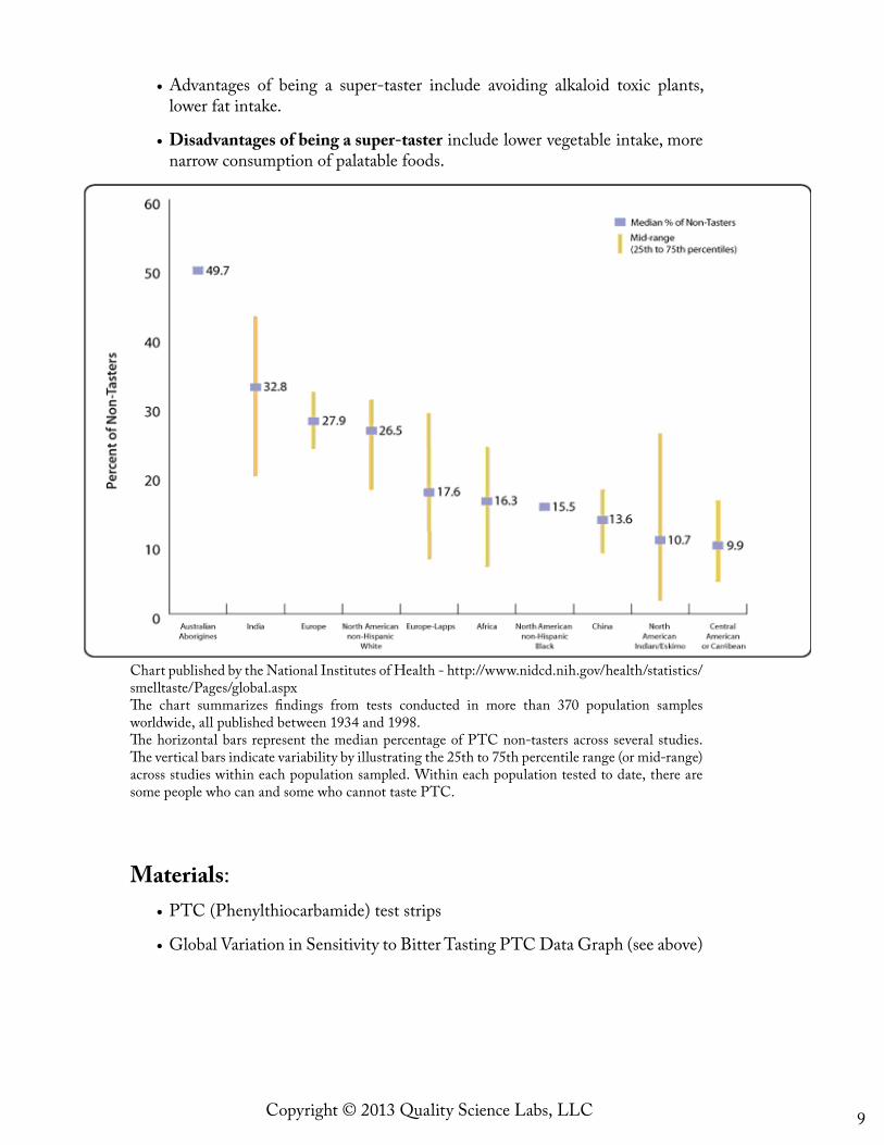
•Advantages of being a super-taster include avoiding alkaloid toxic plants, lower fat intake.

•Disadvantages of being a super-taster include lower vegetable intake, more narrow consumption of palatable foods.

Materials:•PTC (Phenylthiocarbamide) test strips

•Global Variation in Sensitivity to Bitter Tasting PTC Data Graph (see above)

Chart published by the National Institutes of Health - http://www.nidcd.nih.gov/health/statistics/smelltaste/Pages/global.aspxThe chart summarizes findings from tests conducted in more than 370 population samples worldwide, all published between 1934 and 1998.The horizontal bars represent the median percentage of PTC non-tasters across several studies. The vertical bars indicate variability by illustrating the 25th to 75th percentile range (or mid-range) across studies within each population sampled. Within each population tested to date, there are some people who can and some who cannot taste PTC.


Procedures:

1. Using the PTC test strips, press it to your tongue tip. PTC tasters will sense a bitter taste. For the purpose of this exercise, these individuals are considered to be tasters.

2. A decimal number representing the frequency of tasters should be calculated by dividing the number of tasters in the test subject group by the total number of test subjects. This will be p2 + 2pq in the H-W equation.

3. A decimal number representing the frequency of non-tasters (q2 in the H-W equation) should be calculated by dividing the number of non-tasters by the total number of test subjects. Record these numbers in Table 2.1a below.

4. Use the Hardy-Weinberg equation to determine the frequencies (p and q) of the two alleles. The frequency q can be calculated by taking the square root of q2. Once q has been determined, p can be determined because 1 – q = p. Record these values in Table 2.1a for the class.

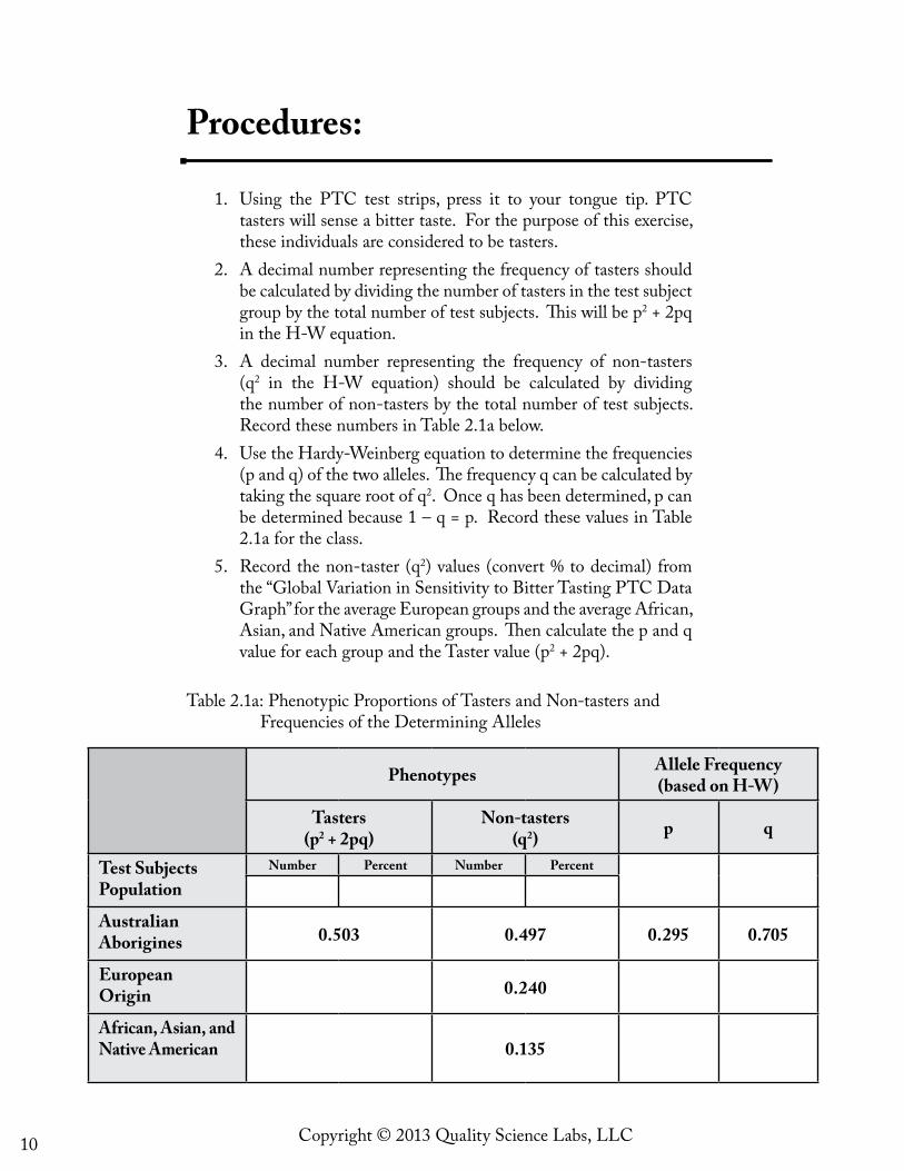
5. Record the non-taster (q2) values (convert % to decimal) from the “Global Variation in Sensitivity to Bitter Tasting PTC Data Graph” for the average European groups and the average African, Asian, and Native American groups. Then calculate the p and q value for each group and the Taster value (p2 + 2pq).

Phenotypes Allele Frequency (based on H-W)

Tasters (p2 + 2pq)

Non-tasters (q2) p q

Test Subjects Population

Number Percent Number Percent

Australian Aborigines 0.503 0.497 0.295 0.705

European Origin 0.240

African, Asian, and Native American 0.135

Table 2.1a: Phenotypic Proportions of Tasters and Non-tasters and Frequencies of the Determining Alleles


Questions:

1. Why do you think people that are homozygous (TT) for the dominant allele have a much stronger bitter taste?

2. How does the class frequency of alleles (TT, Tt, and the tt) compare with the Europeans/North Americans? If there is a significant difference, can you think of some reasons why?

3. How different was the African/Asian/Native American group frequency of alleles to all other groups that you analyzed including your class data?

4. Can you explain why frequencies would be different among different populations globally? Think about what the advantages might be for a higher % of tasters in the population?

5. If the ability to taste bitter compounds conveys a selective advantage, then shouldn't non-tasters have died off long ago? Can you think of any reasons why so many people still carry the non-tasting PTC variant?


Lab Investigation 2.1 A Micro-Evolution Simulation

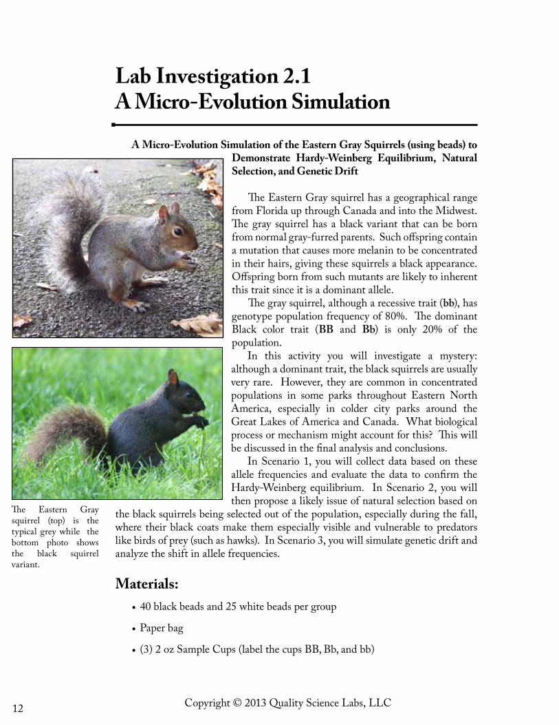
A Micro-Evolution Simulation of the Eastern Gray Squirrels (using beads) to Demonstrate Hardy-Weinberg Equilibrium, Natural Selection, and Genetic Drift

The Eastern Gray squirrel has a geographical range from Florida up through Canada and into the Midwest. The gray squirrel has a black variant that can be born from normal gray-furred parents. Such offspring contain a mutation that causes more melanin to be concentrated in their hairs, giving these squirrels a black appearance. Offspring born from such mutants are likely to inherent this trait since it is a dominant allele.

The gray squirrel, although a recessive trait (bb), has genotype population frequency of 80%. The dominant Black color trait (BB and Bb) is only 20% of the population.

In this activity you will investigate a mystery: although a dominant trait, the black squirrels are usually very rare. However, they are common in concentrated populations in some parks throughout Eastern North America, especially in colder city parks around the Great Lakes of America and Canada. What biological process or mechanism might account for this? This will be discussed in the final analysis and conclusions.

In Scenario 1, you will collect data based on these allele frequencies and evaluate the data to confirm the Hardy-Weinberg equilibrium. In Scenario 2, you will then propose a likely issue of natural selection based on

the black squirrels being selected out of the population, especially during the fall, where their black coats make them especially visible and vulnerable to predators like birds of prey (such as hawks). In Scenario 3, you will simulate genetic drift and analyze the shift in allele frequencies.

Materials:•40 black beads and 25 white beads per group

•Paper bag

• (3) 2 oz Sample Cups (label the cups BB, Bb, and bb)

The Eastern Gray squirrel (top) is the typical grey while the bottom photo shows the black squirrel variant.


Procedures:

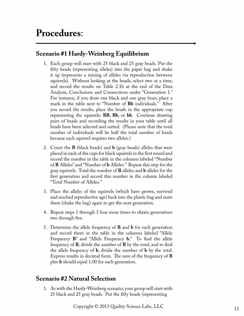
Scenario #1 Hardy-Weinberg Equilibrium 1. Each group will start with 25 black and 25 gray beads. Put the

fifty beads (representing alleles) into the paper bag and shake it up (represents a mixing of alleles via reproduction between squirrels). Without looking at the beads, select two at a time, and record the results on Table 2.1b at the end of the Data Analysis, Conclusions and Connections under “Generation 1.” For instance, if you draw one black and one gray bean, place a mark in the table next to “Number of Bb individuals.” After you record the results, place the beads in the appropriate cup representing the squirrels: BB, Bb, or bb. Continue drawing pairs of beads and recording the results in your table until all beads have been selected and sorted. (Please note that the total number of individuals will be half the total number of beads because each squirrel requires two alleles.)

2. Count the B (black beads) and b (gray beads) alleles that were placed in each of the cups for black squirrels in the first round and record the number in the table in the columns labeled “Number of B Alleles” and “Number of b Alleles.” Repeat this step for the gray squirrels. Total the number of B alleles and b alleles for the first generation and record this number in the column labeled “Total Number of Alleles.”

3. Place the alleles of the squirrels (which have grown, survived and reached reproductive age) back into the plastic bag and mate them (shake the bag) again to get the next generation.

4. Repeat steps 1 through 3 four more times to obtain generations two through five.

5. Determine the allele frequency of B and b for each generation and record them in the table in the columns labeled “Allele Frequency B” and “Allele Frequency b.” To find the allele frequency of B, divide the number of B by the total, and to find the allele frequency of b, divide the number of b by the total. Express results in decimal form. The sum of the frequency of B plus b should equal 1.00 for each generation.

Scenario #2 Natural Selection 1. As with the Hardy-Weinberg scenario, your group will start with

25 black and 25 gray beads. Put the fifty beads (representing


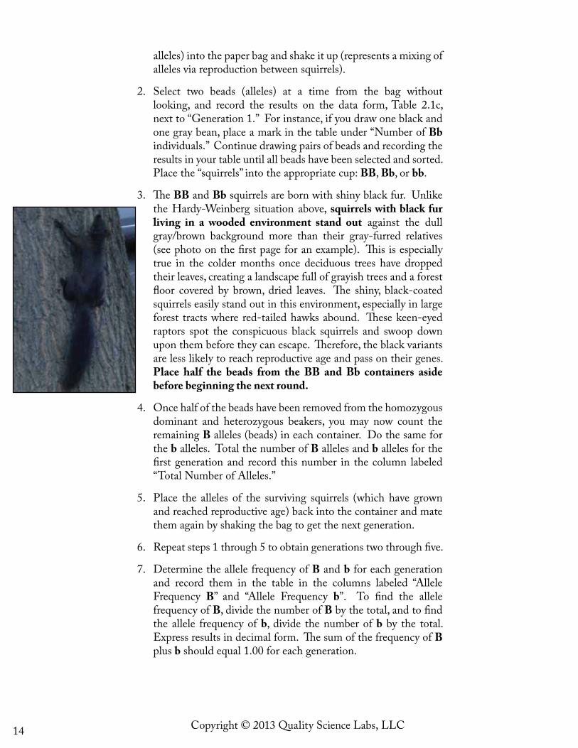
alleles) into the paper bag and shake it up (represents a mixing of alleles via reproduction between squirrels).

2. Select two beads (alleles) at a time from the bag without looking, and record the results on the data form, Table 2.1c, next to “Generation 1.” For instance, if you draw one black and one gray bean, place a mark in the table under “Number of Bb individuals.” Continue drawing pairs of beads and recording the results in your table until all beads have been selected and sorted. Place the “squirrels” into the appropriate cup: BB, Bb, or bb.

3. The BB and Bb squirrels are born with shiny black fur. Unlike the Hardy-Weinberg situation above, squirrels with black fur living in a wooded environment stand out against the dull gray/brown background more than their gray-furred relatives (see photo on the first page for an example). This is especially true in the colder months once deciduous trees have dropped their leaves, creating a landscape full of grayish trees and a forest floor covered by brown, dried leaves. The shiny, black-coated squirrels easily stand out in this environment, especially in large forest tracts where red-tailed hawks abound. These keen-eyed raptors spot the conspicuous black squirrels and swoop down upon them before they can escape. Therefore, the black variants are less likely to reach reproductive age and pass on their genes. Place half the beads from the BB and Bb containers aside before beginning the next round.

4. Once half of the beads have been removed from the homozygous dominant and heterozygous beakers, you may now count the remaining B alleles (beads) in each container. Do the same for the b alleles. Total the number of B alleles and b alleles for the first generation and record this number in the column labeled “Total Number of Alleles.”

5. Place the alleles of the surviving squirrels (which have grown and reached reproductive age) back into the container and mate them again by shaking the bag to get the next generation.

6. Repeat steps 1 through 5 to obtain generations two through five.

7. Determine the allele frequency of B and b for each generation and record them in the table in the columns labeled “Allele Frequency B” and “Allele Frequency b”. To find the allele frequency of B, divide the number of B by the total, and to find the allele frequency of b, divide the number of b by the total. Express results in decimal form. The sum of the frequency of B plus b should equal 1.00 for each generation.


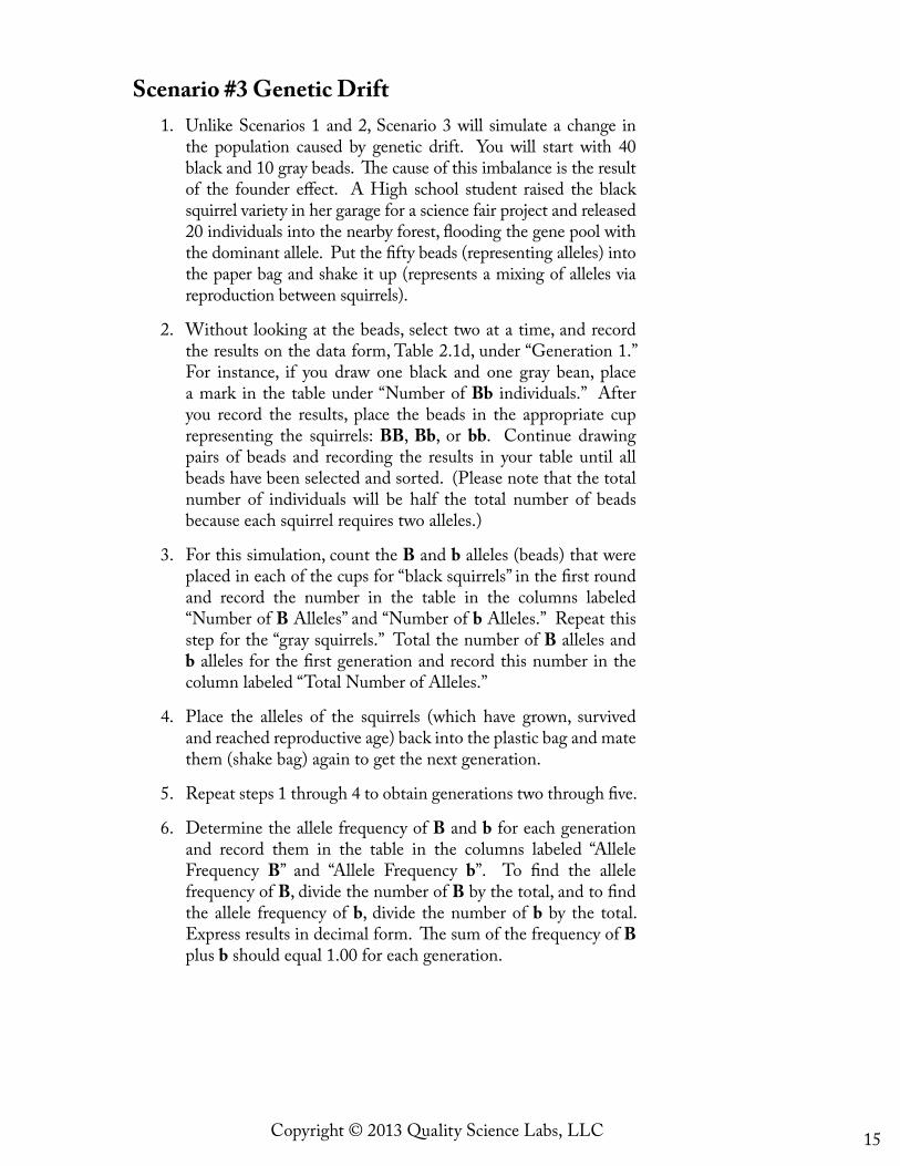
Scenario #3 Genetic Drift 1. Unlike Scenarios 1 and 2, Scenario 3 will simulate a change in

the population caused by genetic drift. You will start with 40 black and 10 gray beads. The cause of this imbalance is the result of the founder effect. A High school student raised the black squirrel variety in her garage for a science fair project and released 20 individuals into the nearby forest, flooding the gene pool with the dominant allele. Put the fifty beads (representing alleles) into the paper bag and shake it up (represents a mixing of alleles via reproduction between squirrels).

2. Without looking at the beads, select two at a time, and record the results on the data form, Table 2.1d, under “Generation 1.” For instance, if you draw one black and one gray bean, place a mark in the table under “Number of Bb individuals.” After you record the results, place the beads in the appropriate cup representing the squirrels: BB, Bb, or bb. Continue drawing pairs of beads and recording the results in your table until all beads have been selected and sorted. (Please note that the total number of individuals will be half the total number of beads because each squirrel requires two alleles.)

3. For this simulation, count the B and b alleles (beads) that were placed in each of the cups for “black squirrels” in the first round and record the number in the table in the columns labeled “Number of B Alleles” and “Number of b Alleles.” Repeat this step for the “gray squirrels.” Total the number of B alleles and b alleles for the first generation and record this number in the column labeled “Total Number of Alleles.”

4. Place the alleles of the squirrels (which have grown, survived and reached reproductive age) back into the plastic bag and mate them (shake bag) again to get the next generation.

5. Repeat steps 1 through 4 to obtain generations two through five.

6. Determine the allele frequency of B and b for each generation and record them in the table in the columns labeled “Allele Frequency B” and “Allele Frequency b”. To find the allele frequency of B, divide the number of B by the total, and to find the allele frequency of b, divide the number of b by the total. Express results in decimal form. The sum of the frequency of B plus b should equal 1.00 for each generation.


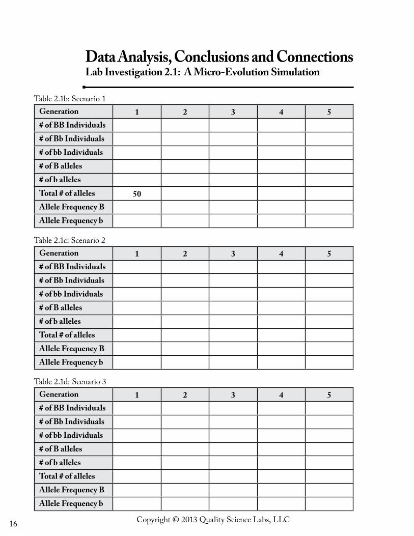
Data Analysis, Conclusions and ConnectionsLab Investigation 2.1: A Micro-Evolution Simulation

Generation 1 2 3 4 5# of BB Individuals# of Bb Individuals# of bb Individuals# of B alleles# of b allelesTotal # of alleles 50Allele Frequency BAllele Frequency b

Table 2.1b: Scenario 1

Generation 1 2 3 4 5# of BB Individuals# of Bb Individuals# of bb Individuals# of B alleles# of b allelesTotal # of allelesAllele Frequency BAllele Frequency b

Table 2.1c: Scenario 2

Generation 1 2 3 4 5# of BB Individuals# of Bb Individuals# of bb Individuals# of B alleles# of b allelesTotal # of allelesAllele Frequency BAllele Frequency b

Table 2.1d: Scenario 3


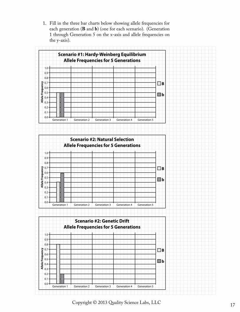
1. Fill in the three bar charts below showing allele frequencies for each generation (B and b) (one for each scenario). (Generation 1 through Generation 5 on the x-axis and allele frequencies on the y-axis).

0.0

0.1

0.2

0.3

0.4

0.5

0.6

0.7

0.8

0.9

1.0

Generation 1 Generation 2 Generation 3 Generation 4 Generation 5

Scenario #1: Hardy-Weinberg EquilibriumAllele Frequencies for 5 Generations

Alle

le F

requ

ency B

b

0.0

0.1

0.2

0.3

0.4

0.5

0.6

0.7

0.8

0.9

1.0


Scenario #2: Natural SelectionAllele Frequencies for 5 Generations

Alle

le F

requ

ency B

b

0.0

0.1

0.2

0.3

0.4

0.5

0.6

0.7

0.8

0.9

1.0


Scenario #2: Genetic DriftAllele Frequencies for 5 Generations

Alle

le F

requ

ency B

b


2. How does the Hardy-Weinberg provide a baseline for identifying how populations change, as a function of changes in their allele frequencies? Reconsider the seven criteria of the Hardy-Weinberg Equilibrium: •Large population. The population must be large to

minimize random sampling errors. •Random mating. There is no mating preference. For

example, an AA male does not prefer an aa female. •No mutation. The alleles must not change. •No migration. Exchange of genes between the population

and another population must not occur. •No natural selection. Natural selection must not favor

any individual.

3. Did your Scenario #1 Hardy-Weinberg experimental data verify the Hardy-Weinberg Equilibrium? If your data was inconsistent, what might contribute to erroneous data?

4. How did the results in Scenario #2 data demonstrate an allele frequency change due to natural selection?


5. What differences were seen in Scenario #3 data due to genetic drift?

6. As you have seen in this activity, gray squirrels predominate due to the fact that they are camouflaged better than their black-coated relatives. However, biologists have measured that black squirrels have 18% lower heat loss in temperatures below -10 degrees Celsius, along with a 20% lower basal metabolic rate, and therefore shiver less (by 11%) compared to the gray variety. How does this study answer why concentrated populations of “black” gray squirrels are found commonly in some northern city parks?


Lab Investigation 2.2 Part 1 - Estimating Allele Frequencies Tutorial

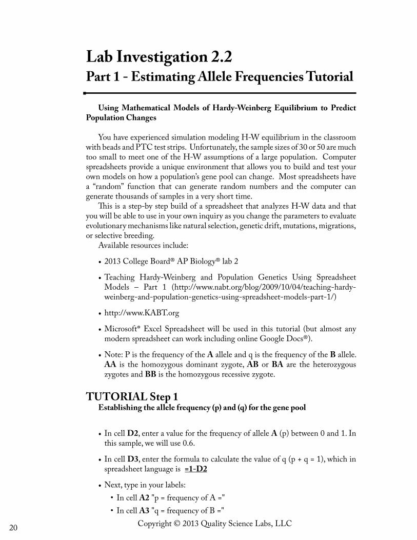
Using Mathematical Models of Hardy-Weinberg Equilibrium to Predict Population Changes

You have experienced simulation modeling H-W equilibrium in the classroom with beads and PTC test strips. Unfortunately, the sample sizes of 30 or 50 are much too small to meet one of the H-W assumptions of a large population. Computer spreadsheets provide a unique environment that allows you to build and test your own models on how a population’s gene pool can change. Most spreadsheets have a “random” function that can generate random numbers and the computer can generate thousands of samples in a very short time.

This is a step-by step build of a spreadsheet that analyzes H-W data and that you will be able to use in your own inquiry as you change the parameters to evaluate evolutionary mechanisms like natural selection, genetic drift, mutations, migrations, or selective breeding.

Available resources include:

•2013 College Board® AP Biology® lab 2

•Teaching Hardy-Weinberg and Population Genetics Using Spreadsheet Models – Part 1 (http://www.nabt.org/blog/2009/10/04/teaching-hardy-weinberg-and-population-genetics-using-spreadsheet-models-part-1/)

•http://www.KABT.org

•Microsoft® Excel Spreadsheet will be used in this tutorial (but almost any modern spreadsheet can work including online Google Docs®).

•Note: P is the frequency of the A allele and q is the frequency of the B allele. AA is the homozygous dominant zygote, AB or BA are the heterozygous zygotes and BB is the homozygous recessive zygote.

TUTORIAL Step 1 Establishing the allele frequency (p) and (q) for the gene pool

• In cell D2, enter a value for the frequency of allele A (p) between 0 and 1. In this sample, we will use 0.6.

• In cell D3, enter the formula to calculate the value of q (p + q = 1), which in spreadsheet language is =1-D2

•Next, type in your labels:• In cell A2 "p = frequency of A ="• In cell A3 "q = frequency of B ="


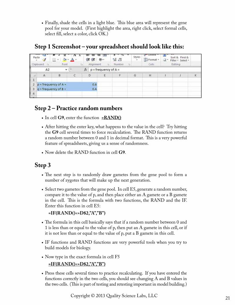
•Finally, shade the cells in a light blue. This blue area will represent the gene pool for your model. (First highlight the area, right click, select formal cells, select fill, select a color, click OK.)

Step 1 Screenshot – your spreadsheet should look like this:

Step 2 – Practice random numbers • In cell G9, enter the function =RAND()

•After hitting the enter key, what happens to the value in the cell? Try hitting the G9 cell several times to force recalculation. The RAND function returns a random number between 0 and 1 in decimal format. This is a very powerful feature of spreadsheets, giving us a sense of randomness.

•Now delete the RAND function in cell G9.

Step 3 •The next step is to randomly draw gametes from the gene pool to form a

number of zygotes that will make up the next generation.

•Select two gametes from the gene pool. In cell E5, generate a random number, compare it to the value of p, and then place either an A gamete or a B gamete in the cell. This is the formula with two functions, the RAND and the IF. Enter this function in cell E5:

=IF(RAND()<=D$2,”A”,”B”)

•The formula in this cell basically says that if a random number between 0 and 1 is less than or equal to the value of p, then put an A gamete in this cell, or if it is not less than or equal to the value of p, put a B gamete in this cell.

• IF functions and RAND functions are very powerful tools when you try to build models for biology.

•Now type in the exact formula in cell F5=IF(RAND()<=D$2,”A”,”B”)

•Press these cells several times to practice recalculating. If you have entered the functions correctly in the two cells, you should see changing A and B values in the two cells. (This is part of testing and retesting important in model building.)


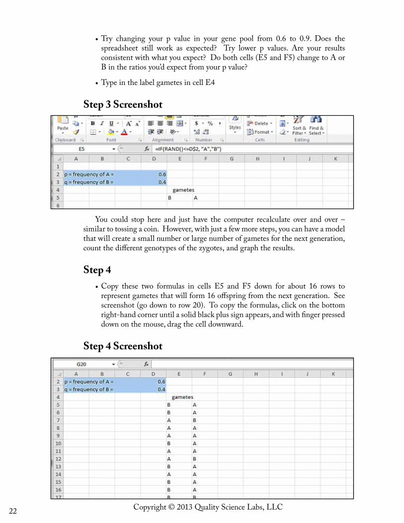
•Try changing your p value in your gene pool from 0.6 to 0.9. Does the spreadsheet still work as expected? Try lower p values. Are your results consistent with what you expect? Do both cells (E5 and F5) change to A or B in the ratios you’d expect from your p value?

•Type in the label gametes in cell E4

Step 3 Screenshot

You could stop here and just have the computer recalculate over and over – similar to tossing a coin. However, with just a few more steps, you can have a model that will create a small number or large number of gametes for the next generation, count the different genotypes of the zygotes, and graph the results.

Step 4 •Copy these two formulas in cells E5 and F5 down for about 16 rows to

represent gametes that will form 16 offspring from the next generation. See screenshot (go down to row 20). To copy the formulas, click on the bottom right-hand corner until a solid black plus sign appears, and with finger pressed down on the mouse, drag the cell downward.

Step 4 Screenshot


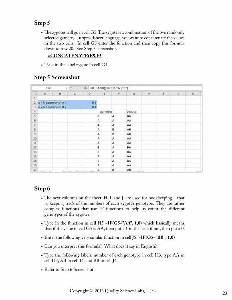
Step 5•The zygotes will go in cell G5. The zygote is a combination of the two randomly

selected gametes. In spreadsheet language, you want to concatenate the values in the two cells. In cell G5 enter the function and then copy this formula down to row 20. See Step 5 screenshot.

=CONCATENATE(E5,F5

•Type in the label zygote in cell G4

Step 5 Screenshot

Step 6•The next columns on the sheet, H, I, and J, are used for bookkeeping – that

is, keeping track of the numbers of each zygote’s genotype. They are rather complex functions that use IF functions to help us count the different genotypes of the zygotes.

•Type in the function in cell H5 =IF(G5=”AA”, 1,0) which basically means that if the value in cell G5 is AA, then put a 1 in this cell; if not, then put a 0.

•Enter the following very similar function in cell J5 =IF(G5=”BB”, 1,0)

•Can you interpret this formula? What does it say in English?

•Type the following labels: number of each genotype in cell H3, type AA in cell H4, AB in cell I4, and BB in cell J4

•Refer to Step 6 Screenshot.


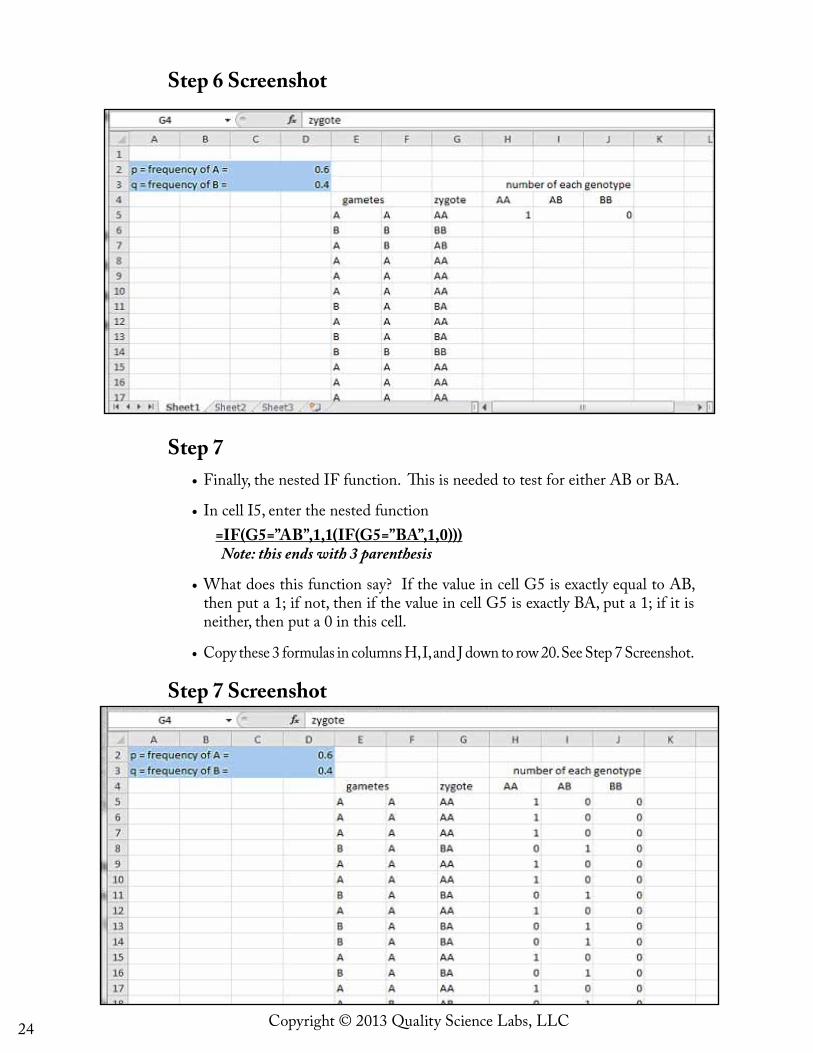
Step 6 Screenshot

Step 7•Finally, the nested IF function. This is needed to test for either AB or BA.

• In cell I5, enter the nested function=IF(G5=”AB”,1,1(IF(G5=”BA”,1,0)))Note: this ends with 3 parenthesis

•What does this function say? If the value in cell G5 is exactly equal to AB, then put a 1; if not, then if the value in cell G5 is exactly BA, put a 1; if it is neither, then put a 0 in this cell.

•Copy these 3 formulas in columns H, I, and J down to row 20. See Step 7 Screenshot.

Step 7 Screenshot


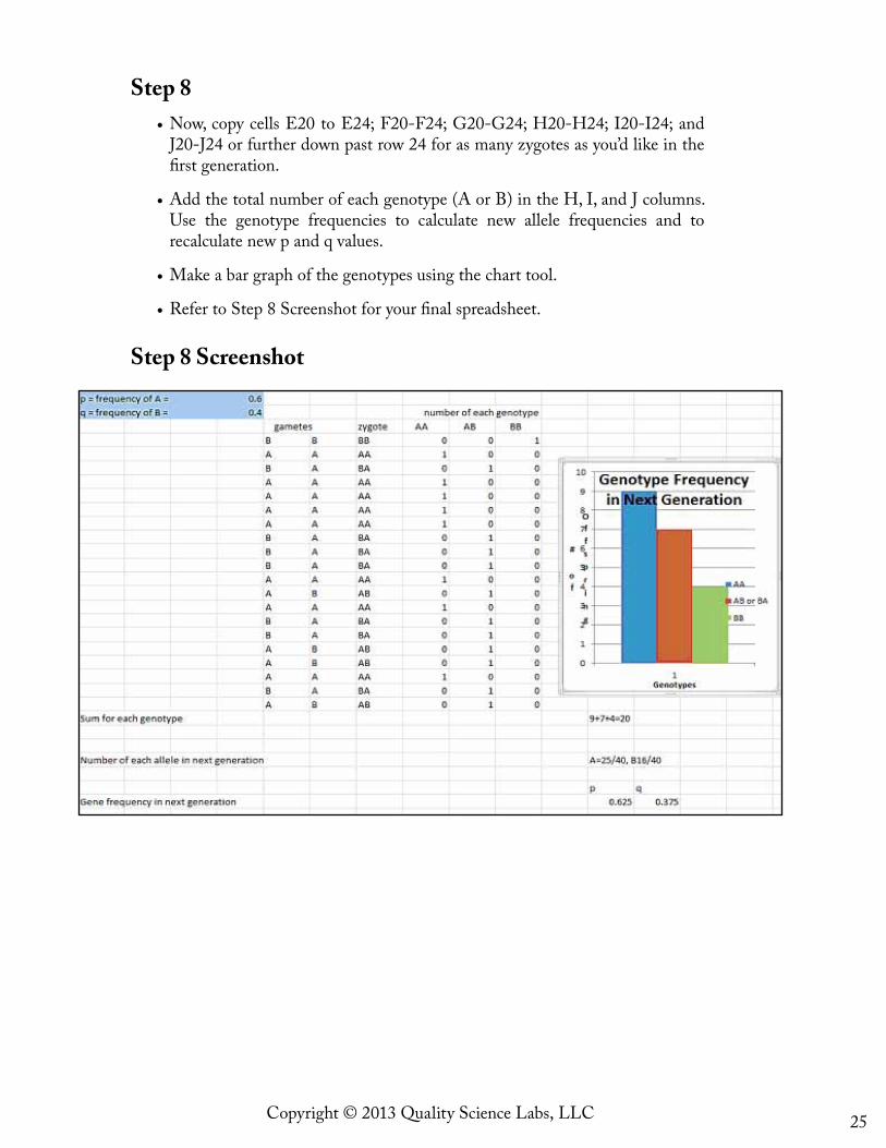
Step 8•Now, copy cells E20 to E24; F20-F24; G20-G24; H20-H24; I20-I24; and

J20-J24 or further down past row 24 for as many zygotes as you’d like in the first generation.

•Add the total number of each genotype (A or B) in the H, I, and J columns. Use the genotype frequencies to calculate new allele frequencies and to recalculate new p and q values.

•Make a bar graph of the genotypes using the chart tool.

•Refer to Step 8 Screenshot for your final spreadsheet.

Step 8 Screenshot


Part 2 - Student Guided Inquiry

Seven Steps to Model Building in Biology using the Hardy-Weinberg Spreadsheet Modeling

A model is a simplification of the real world. Every model has assumptions built in so as you use your computer model, you need to constantly evaluate the assumptions that were made as you interpret the results.

There are seven key steps to model building in biology (Otto and Day, 2007) 1. Formulate the question. Why don’t recessive alleles disappear

from a population gene pool? What about recessive alleles that persist at higher than normal expected rates (like Sickle-cell anemia in malaria infested areas of the world)? What about Cystic fibrosis, a recessive trait. Why does it stay in the population? Why is the recessive gray squirrel (from Pre-lab) at 80% in the population and the dominant black squirrel only at 20%? How do allele frequencies change in a population?

2. Determine the basic ingredients. What are your basic assumptions when looking at how allele frequencies change? Assume that all the organisms are diploid (A and B alleles) and that they all reproduce. Gametes are selected at random for next generation and the population is large (has an infinite gene pool).

3. Qualitatively describe the biological system. Draw a life cycle of the life stages in the population. (Hint: gametes in gene pool, random mating, zygotes, juveniles, and adults) What are the assumptions? They should look like H-W assumptions (see background info at beginning of this unit). You will choose one of these assumptions to change your gene pool in your guided inquiry (mutation, migration, natural selection, genetic drift, selective mating, etc).

4. Quantitatively describe the biological system (spreadsheet). This is where the H-W equilibrium formula is applied where p = the frequency of the A allele and q = the frequency of the B allele in your spreadsheet. The formula that predicts the next generation genotypes will also be p2 + 2pq + q2 = 1.

5. Analyze the equations. The H-W equilibrium says that the allele frequencies in each generation do not change IF there are no forces acting on the population.

6. Perform checks and balances. 7. Relate the results back to the question.


Now you are ready to design your own inquiry investigation using the spreadsheet you developed based on the Hardy-Weinberg equilibrium.

Here are three choices to consider using your spreadsheet: 1. Grey/Black squirrels from Lab Investigation 2.1

•Change the allele frequencies to more extreme. You could plug in the values for the Gray and Black squirrel from Pre-lab (p=.20 and q=.80).

•Use your spreadsheet to add four more generations by plugging in each generation’s newly calculated allele % to your gene pool (original would be p = .20 and q=.8; start your F1 first generation with your calculated results from your spreadsheet at the bottom – your new p and q at the top in a new gene pool). Continue each generation to plug in the new calculated p and q from the previous generation.

•Compare your computer data results to your classroom results. Are there any significant differences? If so, why?

2. What if the recessive zygote was lethal? Modify your spreadsheet so that every time a BB showed up, it was eliminated and run it for 10 generations. This is a real scenario for Bengal tigers living in highland cold mountains of India The recessive trait is no hair. This is lethal to the tigers. Would the recessive trait be eliminated from the gene pool eventually? If so, how long would it take?

3. How could you build into your spreadsheet natural selection preferences for allele A? Run it for 5 generations and compare to your natural selection activity in the Lab Investigation 2.1. How does the data compare? How did the allele frequencies change?

ap biology lab-02

Documents

biological evolution

term evolution

chemical evolution

planetary evolution

background evolution

universal evolution

micro evolution

effects of evolution