aperturbationapproachtolargeeddysimulationofwave-induced

INTERNATIONAL JOURNAL FOR NUMERICAL METHODS IN FLUIDS

A perturbation approach to large eddy simulation of wave-inducedbottom boundary layer flows

Jeffrey C. Harris∗,† and Stéphan T. Grilli

Department of Ocean Engineering, University of Rhode Island, Narragansett, RI 02882, U.S.A.

SUMMARY

We present the development, validation, and application of a numerical model for the simulation of bottomboundary layer (BL) flows induced by arbitrary finite amplitude waves. Our approach is based on couplinga ‘near-field’ local Navier–Stokes (NS) model with a ‘far-field’ inviscid flow model, which simulates largescale incident wave propagation and transformations over a complex ocean bottom, to the near-field, bysolving the Euler equations, in a fully nonlinear potential flow boundary element formalism. The inviscidvelocity provided by this model is applied through a (one-way) coupling to a NS solver with large eddysimulation (LES), to simulate near-field, wave-induced, turbulent bottom BL flows (using an approximatewall boundary condition by assuming the existence of a log-sublayer). Although a three-dimensional (3D)version of the model exists, applications of the wave model in the present context have been limited totwo-dimensional (2D) incident wave fields (i.e. long-crested swells), while the LES of near-field wave-induced turbulent flows is fully 3D. Good agreement is obtained between the coupled model results andanalytic solutions for both laminar oscillatory BL flow and the steady streaming velocities caused bya wave-induced BL, even when using open boundary conditions in the NS model. The coupled modelis then used to simulate wave-induced BL flows under fully nonlinear swells, shoaling over a slopingbottom, close to the breaking point. Finally, good to reasonable agreement is obtained with results of well-controlled laboratory experiments for rough turbulent oscillatory BLs, for both mean and second-orderturbulent statistics. Copyright ! 2011 John Wiley & Sons, Ltd.

Received 13 September 2010; Accepted 23 January 2011

KEY WORDS: Navier–Stokes; marine hydrodynamics; boundary element methods; finite-volumemethods; potential flow; turbulent flow; shallow water; nonlinear dynamics; validation

1. INTRODUCTION

Complex turbulent flows can be accurately modeled by solving Navier–Stokes (NS) equations,either by directly resolving all scales of turbulent motion (DNS, e.g. [1]) or in a time- or space-averaged sense, in combination with a turbulence closure scheme (e.g. [2]). Many methods andalgorithms have been proposed for doing so (which have been detailed elsewhere). Here, wepresent the integration and application of a previously proposed large eddy simulation (LES,[3]) as a component of a new hybrid modeling approach for simulating wave-induced boundarylayer (BL) flows. While more amenable to large size and high Reynolds number computationsthan DNS, the LES of complex three-dimensional (3D) flows over large and/or finely discretizeddomains still represents quite a formidable problem, despite the continual increase in computerperformance. Hence, one must always try and limit the computational domain size to that necessaryand sufficient for solving a given problem or physics, or even dimensionality (e.g. two-dimensional,

∗Correspondence to: Jeffrey C. Harris, Department of Ocean Engineering, University of Rhode Island, Narragansett,RI 02882, U.S.A.

†E-mail: [email protected]

Copyright ! 2011 John Wiley & Sons, Ltd.

Int. J. Numer. Meth. Fluids 2012; 68:1574–1604Published online 201 in Wiley Online Library (wileyonlinelibrary.com). DOI: 10.1002/fld. 38 April 1 255

2D, versus 3D). For coastal wave dynamics problems, which typically extend over multiple spatialand temporal scales (e.g. from deep water to the shoaling and surf zones), it is often sufficientlyaccurate to use a simpler approach for a large part of the domain, to propagate and transformwaves to the region of specific interest, in which 3D-NS simulations can then be more realisticallyperformed. Using a 3D-NS solver for the entire domain would not only be computationallyprohibitive, but would likely yield less accurate results (due to under-discretization and excessivenumerical diffusion), than for instance much less costly inviscid flow solvers (even fully nonlinear,e.g. [4–6]) or higher order Boussinesq equation models (e.g. FUNWAVE [7, 8]). Furthermore, forlong-crested swell, nearshore wave transformations can often be assumed to be 2D.

This has provided a rationale for the development of hybrid modeling approaches, in whichdifferent types of models are coupled and used in various regions of the fluid domain, where theyare both more efficient and adapted to the dominant physics and scales in each given region (see,e.g. [9] for a review). Such models have already been applied to surfzone dynamics problems (e.g.[10–12]), wave structure interaction problems (e.g. [13]), and to model wave-induced flows andresulting sediment suspension over objects on the seabed (e.g. [14]). In the latter work, a so-callednumerical wavetank (NWT) solving fully nonlinear potential flow (FNPF) equations was coupledto a 3D-LES in a somewhat heuristic manner.

As indicated above, the LES method used here is based on the approach of Zang et al. [3],who initially developed the NS solver and one of the subgrid scale (SGS) turbulence models beingused here (dynamic mixed model, DMM) to study coastal upwellings [15, 16], and later modifiedthe latter to study turbulent lid-driven cavity flows [3]; further modifications were done to studybreaking interfacial waves [17] and suspended sediment transport [18, 19]. As discussed above,Gilbert et al. [14] coupled Zang et al.’s model to a 2D-NWT, to study wave-induced BL flowsand sediment transport, through the addition to the NS model equations of the dynamic pressuregradient (equivalent to a body force) caused by waves, computed in the NWT. With this model,they were able to realistically (albeit quite qualitatively) simulate the suspended sediment transportover a partly buried circular obstacle, for a few periodic wave cycles. This implementation didnot move beyond such simple cases, both because of the imperfect coupling between the LES andFNPF model equations and severe limitations of the LES grid size (as the code was not designedto take advantage of recent advances in distributed memory computing clusters).

We report here on more recent developments (in formalism, accuracy, and efficiency) of thetechniques used in Gilbert et al. [14]. Specifically, in a new proposed hybrid approach, a modifiedand extended version of Zang et al.’s [3] 3D-NS-LES model is used in a perturbation schemeto simulate near-field, fine scale, turbulent bottom BL flows induced by arbitrary finite amplitudewaves (i.e. 2D swells), whose propagation and nearshore transformation over larger scale bottomfeatures, are modeled from the far- to the near-field in an inviscid flow model (i.e. NWT), whichsolves Euler equations in a FNPF formalism. The perturbation scheme consists in first dividing thetotal pressure and velocity fields into inviscid and viscous perturbation parts and then to rewriteNS equations for the perturbation fields only; this yields new forcing terms, which are functionof inviscid flow fields representing incident wave forcing (e.g. similar to Kim et al. [20] andAlessandrini [21]). Moreover, in this approach, the computational domains for both NS-LES andFNPF models fully overlap, which makes it easy passing information from one domain to theother, although here we will just illustrate a one-way coupling, from large to fine scales flows.Additionally, this coupling method is very relevant to the physics of wave-induced flow problemssince, for non-breaking waves and outside of BLs, the bulk of the flow is nearly inviscid.

It should be noted that developments of Zang’s LES also continued independently to thosepresented here in relation to the hybrid coupled modeling approach. Thus, Cui and Street [22]implemented a parallelized version of the code, which allowed for much larger computationaldomains. Grilli et al. [23] used this latter version to begin testing its suitability for wave-inducedBLs, with the goal of again coupling it to an FNPF-NWT. A completely separate developmentof Cui and Street’s code for bedform evolution was done by Chou and Fringer [24, 25]. Other,unrelated research groups, have also been actively studying the application of LES to turbulentoscillatory BLs (e.g. [26, 27]). While the LES, SGS models, and perturbation method presented


1575PERTURBATION APPROACH TO LARGE EDDY SIMULATION

Int. J. Numer. Meth. Fluids 2012; 68:1574–1604DOI: 10.1002/fld

here have all been used in one form or another by previous researchers, the particular integrationof these three components into an accurate and efficient parallelized implementation, well suited tocoastal engineering problems, is new and unique. Additionally, the coupling to a 2D-FNPF-NWT,and potentially in future developments to a similar 3D-NWT (e.g. [28]) makes it possible to use avariety of fully realistic nonlinear and irregular wave forcings, besides the commonly used simpleoscillatory or linear wave flows (see e.g. [29]).

In summary, in this paper, we present recent improvements and validation of a new hybridmethod applied to simulating oscillatory and wave-induced BL flows with a 3D-LES. For validationwe compare simulation results to analytic solutions of laminar flows and to experimental resultsof rough turbulent oscillatory BLs. In our hybrid/perturbation approach, the total velocity andpressure fields are expressed as the sum of irrotational (thus kinematically inviscid) and near-fieldviscous perturbations above a rigid seafloor. The NS equations are formulated and solved for theperturbation fields only, which are forced by additional terms representing the incident fields. Inthe present applications, these are given either analytically or numerically obtained in a coupled2D-FNPF-NWT.

2. OSCILLATORY BL FLOW PHYSICS AND MODELS

A wide range of approaches besides LES has been proposed for modeling turbulent oscillatoryBLs, often in the context of wave-induced flow on the seafloor. The earliest approaches weremerely empirical relationships or were based on a time-varying logarithmic BL assumption. Kajiura[30] considered a piecewise varying eddy viscosity distribution. Grant and Madsen [31] used amixing-length approach where eddy viscosity was proportional to the height above the bed. Theseand other similar works all reported good agreement with mean flow measurements, but did notmodel turbulent statistics well if at all. Only later models, like Trowbridge and Madsen’s [32]or Davies’s [33], considered a time-varying eddy viscosity, which is experimentally observed.More recently, Reynolds-averaged NS models (RANS) of turbulent oscillatory BLs have been usedextensively which provided reasonable to good agreement with experiment for both mean flow andsecond-order turbulent statistics (e.g. [34–40]). In those, many different turbulence models wereused, from Saffman’s energy-vorticity turbulence model, used by Blondeaux, to a high Reynoldsnumber k−! model used by Justesen, or the two-equation turbulence closure of Chien, used byThais et al.

The flow in a purely oscillatory BL over a solid horizontal wall is driven by a periodic pressuregradient. In the simplest case the forcing flow is represented by a sinusoidal free-stream (inviscid)velocity given by uI

i ="i1U0 sin#t , where U0 is the amplitude and # the angular frequency. Faraway from the wall, water particles follow the free-stream and oscillate with an amplitude on theorder A=U0/#. In the BL, the flow additionally depends on the kinematic viscosity, $ and, forrough boundaries, on the Nikuradse roughness length, ks . The BL flow regime is thus dependenton two non-dimensional numbers: (i) a relative roughness, A/ks and (ii) the Reynolds number,U0A/$. Figure 1 shows various regime regions identified based on values of those two parameters.Various authors (e.g. [34, 41, 45]) have proposed slightly different or additional regions, but ingeneral the flow regime can either be described as laminar, smooth turbulent, rough turbulent, ortransitional. To a first order, wave-induced oscillatory BLs can be characterized in the same way.In this paper, we will consider both laminar and rough turbulent conditions.

Many measurements of turbulent oscillatory BLs have been reported, usually made in anoscillatory water tunnel (e.g. [44]), or a reciprocating wind tunnel (e.g. [46]), resulting in manyadvances in understanding oscillatory BLs. Measurements from wavetanks (e.g. [42]) are possible,but except in the largest wavetanks it is not usually possible to reproduce the high Reynolds numberflows that are present in the ocean. Thus, Jonsson and Carlsen [44] measured mean flow velocitiesover rough walls in an oscillatory water tunnel for two different rough turbulent tests. Theyfound that the velocity at points just above the rough bed could be well described by a log-layer


1576 J. C. HARRIS AND S. T. GRILLI


Figure 1. Oscillatory BL flow regimes as a function of Reynolds number and relative roughness, asestimated by Kamphuis [41] and overview of conditions observed in selected experiments (•—Sleath

[42]; ◦—Jensen et al. [43]; and $—Jonsson and Carlsen [44]).

assumption. Hino et al. [46] measured mean flow velocities, turbulent intensities, Reynolds stressesand turbulent-energy production rates for oscillatory BLs over a smooth wall. Interestingly, theyfound that the spectral decay of the turbulent energy in the decelerating phase is steeper than the5/3 power law of the Kolmogorov spectrum (see e.g. Pope [47] for a general description of spectralanalysis of turbulence). Sleath [48] was one of the first to measure both turbulent intensity andmean flow velocity for oscillatory BLs over rough surfaces. Notably Sleath found that the time-averaged eddy viscosity near the rough bed was negative, meaning that the turbulent momentumis transported against the mean velocity gradient, which implies that the turbulent kinetic energyproduction is negative. Sleath suggested that this was due to jets of fluid moving away from thewall near flow-reversals. Jensen et al. [43] measured mean flow velocity and turbulent intensityover both smooth and rough walls.

Although far from the boundary wave-induced BLs tend toward an inviscid solution, wave-induced BLs differ from purely uniform oscillatory BLs in that weak vorticity is present at moderatedistances from the seabed. While to a first order this is typically insignificant, it does induce asteady streaming velocity. Longuet-Higgins derived a theory describing steady streaming velocityprofiles for wave-induced laminar BL flows [49] or with time-invariant eddy viscosity distributions[50]. Trowbridge and Madsen [32] developed a model which instead considered a time-varyingeddy viscosity distribution. Since then, Reynolds-averaged approaches have been commonly usedfor representing wave-induced BLs (e.g. [51–55]). A more practical model of drift over veryrough beds was developed by Davies and Villaret [56] where the dominant process is vortexshedding as opposed to random turbulence. Recently, Myrhaug and Holmedal [57] derived thesteady streaming induced by random waves, in both laminar and turbulent conditions. Others havefocused on the effects of wave asymmetry. Scandura [58] numerically modeled steady streamingfor a transitionally turbulent BL forced by a pressure gradient with two harmonics. Holmedal andMyrhaug [59] have considered the combination of Longuet-Higgins steady streaming and waveasymmetry, as well as their relative contributions to the overall steady streaming velocities fordifferent parameters and for both sinusoidal and Stokes second-order waves. Note, in the presentapproach, the coupling of the 3D-LES to the fully nonlinear NWT, which also allows representingarbitrary bottom bathymetry, makes it possible to simulate the wave-induced forcing flow from




fully realistic, strongly nonlinear (near-breaking), shoaling waves, which are both trough-crest andfront-rear asymmetric.

When deriving a theory for wave-induced steady streaming over constant depth in a very thin BL(as compared with the wavelength), only the horizontal component of the inviscid forcing needsto be considered [60]. In this context, earlier theoretical and numerical research has focused onsinusoidal or second-order Stokes waves. Under sinusoidal waves, the steady streaming velocityis always in the direction of wave propagation [49], whereas under second-order Stokes waves,streaming is reduced or may be in the opposite direction [59]. Higher order wave forcing of courseprovides more realistic conditions, which, as indicated above, can be obtained from simulationsin an FNPF-NWT, such as Grilli and Subramanya’s [4] 2D-NWT. In the latter, as in many similarNWTs, continuity is satisfied by solving Laplace’s equation for the velocity potential with aboundary element method (BEM), and the nonlinear kinematic and dynamic free surface boundaryconditions are integrated in time with a mixed Eulerian–Lagrangian (MEL) scheme. The MELscheme was first introduced in this context by Longuet-Higgins and Cokelet [61] and allowed forsimulating overturning waves. (A similar 3D-NWT was developed by Grilli et al. [28].) In thiswork, we compare the effects of a variety of forcing functions on the oscillatory BL flow.

While Longuet-Higgins [49] validated his theory using earlier measurements, Russell and Osorio[62] and Collins [63] further confirmed that the drift velocity at the edge of the BL matchedLonguet-Higgin’s theory for laminar flows over a flat bed. Because this velocity was independentof viscosity, Longuet-Higgins [50] suggested that, for a constant eddy viscosity, the same resultwould hold in turbulent conditions. Johns [64] extended this argument to vertically varying buttime-independent eddy viscosity models, typical of the time. Collins’ [63] measurements suggestedthat this was not true at higher Reynolds numbers, which has since been confirmed by Brebneret al. [65], Bijker et al. [66], and van Doorn [67]. More recent studies have focused on othereffects in the BL. The effect of wave asymmetry acts opposite to the effect of Longuet-Higginssteady streaming, as has been studied by Ribberink and Al-Salem [68] in an oscillating watertunnel. Many studies are focused on either flat seabeds or naturally occurring bedforms. Marin[69] studied Eulerian drift for progressive waves over a rippled bed in the transitionally turbulentregime, and found that the Davies and Villaret [56] model for turbulent flow could be adjusted tohandle transitionally turbulent conditions.

3. GOVERNING EQUATIONS

NS equations for an incompressible, isothermal, Newtonian fluid read as:

!ui!xi

=0 (1)

!ui!t

+ !!x j

(uiu j +

p%

"ij−$!ui!x j

)=0 (2)

where ui and p are the water velocity and dynamic pressure, respectively, in a fluid of density %and kinematic viscosity $. We adopt the indicial tensor notation convention, with x3 denoting avertical distance measured from some reference point.

Let us denote by (uIi , pI ) the velocity and pressure fields of the ocean wave flow, considered to

be inviscid outside of thin BLs. Such flows are well described by Euler equations:

!uIi

!xi=0 (3)

!uIi

!t+ !

!x j

(uIi u

Ij +

pI%

"ij

)=0 (4)




Let us then introduce a decomposition of the total viscous flow into the sum of the latter inviscidfree-stream flow and a defect or perturbation flow, of velocity uP

i and pressure pP :

ui =uIi +uP

i (5)

p= pI + pP (6)

Replacing Equations (5) and (6) into Equations (1) and (2), and subtracting Equations (3) and (4),we derive the governing equations for the perturbation fields as:

!uPi

!xi=0 (7)

!uPi

!t+ !

!x j

(uiu j −uI

i uIj +

pP%

"ij−$!ui!x j

)=0 (8)

Here, the perturbation is defined in a region encompassing the near-field bottom BL of interest.Although formally different, for the range of problems studied here, these equations can be

shown to be equivalent to the forcing of the total flow with the inviscid wave dynamic pressuregradient proposed by Gilbert et al. [14], expressed as:

!ui!xi

=0 (9)

!ui!t

+ !!x j

(uiu j +

pP%

"ij−$!ui!x j

)=−1

%!pI!x j

(10)

There are two key advantages, however, to the current approach, as compared with this earlier work:(1) boundary conditions can be more clearly and accurately defined for the viscous perturbation(i.e. as vanishing or using a radiation condition away from the wall); and (2) only the inviscidvelocity is needed in the NS forcing terms rather than the dynamic pressure gradient.

By applying a spatial-average operator (overbar) to the NS equations we obtain the momentumequation for the resolved perturbation as

!u Pi

!xi=0 (11)

!u Pi

!t+ !

!x j

(ui u j −uI

i uIj +

pP%

"ij−$!ui!x j

+&ij

)=0 (12)

where &ij is the SGS stress defined as:

&ij=uiu j − ui u j (13)

Note that, typically, SGS models only consider the deviatoric stress &ij−&kk/3, because the resolvedturbulent pressure, p∗, is different from the resolved hydrodynamic pressure with:

p∗

%= p

%+ 13&kk (14)

For the SGS models considered here, we define

&ij−"ij3

&kk=−2$T Sij+Cr

(Lmij −

"ij3Lmkk

)(15)

where $T is the eddy viscosity, Sij is the resolved shear strain rate, Lmij is the modified Leonard

term, and Cr is a constant coefficient (either one or zero, depending on the SGS decompositionused).




3.1. Discretization

The governing equations are discretized in 3D as in Cui and Street [22], i.e. using a finite-volumeformulation with second-order accuracy in both time and space on a non-staggered grid. Quadraticupstream interpolation for convective kinematics (QUICK) [70] is used to discretize the convectiveterms of the fluid flow, and second-order centered differences are used for the remaining terms.The convective terms are time integrated using the second-order Adams–Bashforth technique, andthe diffusive terms with a second-order implicit Crank–Nicolson scheme. The Poisson equationfor the pressure field is solved with a multigrid technique. Note that in our hybrid approach, theinviscid velocity field is obtained directly from another model—in this paper, a theoretical solutionor a 2D-NWT—and is not subject to the numerical errors of the NS solver.

For all the test cases that are considered here, the computational domain is a box, L1 long inthe streamwise direction, L2 wide in the spanwise direction, and L3 high in the vertical direction.The corresponding number of gridpoints are N1, N2, and N3, respectively.

For post-processing, it is useful to define variables in terms of integrals that, when discretizedare sums, e.g. ensemble averages. Thus, for an arbitrary variable q that is aperiodic, the averageover a horizontal plane is:

〈q〉(x3)=1

L1L2

∫ ∫q dx1 dx3 (16)

calculated as,

〈q〉([x3] j )=1

N1N2

∑i

∑k[q]i, j,k (17)

where here the additional subscripts []i, j,k are grid indices (with e.g. i varying from 1 to N1),whereas for periodic field variables, an ensemble average can be made more accurate by alsoaveraging over several periods (e.g. 〈q〉(x3)=(1/N )(1/L1L2)

∑Nn=1

∫ L10

∫ L20 q(x1, x2, x3, t+nT/2)

dx1 dx2 or 〈q〉(x3)= (1/N )(1/L1L2)∑N

n=1(−1)n∫ L10

∫ L20 q(x1, x2, x3, t+nT/2)dx1 dx2 depending

on whether the field variable is periodic or antiperiodic, such as the turbulent intensity or the meanvelocity, respectively).

In theoretical models, oscillatory BLs are often considered to be ‘infinitely long’, which wouldcorrespond to a half-plane or half-space. This may represent physical circumstances quite well butis not practical in a numerical model where we want to limit the domain size to limit computationalrequirements. Hence, assuming the flow is statistically homogenous in a direction, we can applyperiodic boundary conditions, with the premise that velocity fluctuations a half-domain away arecompletely uncorrelated with one another. Such space-periodicity conditions will be used for someof the applications presented here.

While the numerical method is designed to handle any structured 3D grid, here we limit ourconsideration to two types—regular grids in each direction and regular grids with exponentialstretching in the vertical direction. The latter is based on a stretching ratio based on the verticaldistance between adjacent gridpoints (e.g. a 1.1-stretching ratio would correspond to a 10% increasein cell size with each step in the vertical direction).

Note that this vertical stretching induces a large aspect ratio for the cells near the boundary.Consider a grid with a seabed of height h(x1, x2), and vertical grid spacing !x3. From a verticalprofile it may appear that eddies of O(!x3) are resolved, for example an aspect ratio of 10:1 thegrid filter acts on a volume of approximately O(102!x33 ), though near-wall eddies are expectedto be O(2'(x3−h)) across, so turbulent eddies near the surface are not resolved (e.g. when2'10−2/3!!x3/(x3−h)). These estimates are most accurate for flat seabeds, but analogous argu-ments can be made for complex bathymetry. Thus we expect an underprediction of turbulentintensity near the wall, and a need to augment the SGS stresses. The method used is described inthe following section.




3.2. Bottom boundary condition

In all cases considered here, the bottom boundary condition is a no-flux condition with a shearstress applied depending on flow conditions, i.e.

&w =%$[

!utan!n

]

x3=h(x1,x2)(18)

where n is the normal direction to the wall, utan is the resolved velocity tangential to the wall,and &w is the wall shear stress. In the BL theory, the latter is typically defined as a function of thefriction velocity u∗, as: &w =%u2∗, which yields

[!u!n

]

x3=h(x1,x2)= 1

$u2∗ (19)

Combining this with the condition that the eddy viscosity is zero along the bed, the boundarycondition can be implemented as a purely viscous wall stress. Numerically, this velocity gradientcondition is implemented through using layers of additional (ghost) cells, located outside of thedomain. We apply one of the two boundary friction velocity models, depending on the application.In each case we evaluate them for the gridpoints adjacent to the boundary (e.g. over a flat bed, atx3=h(x1, x2)+!x3/2). To be unambiguous for curved seabeds, we specify z1 to be the distanceof the center of the first grid cell to the boundary.

For laminar tests, we consider a no-slip condition such that:

u∗ =

√utan$z1

(20)

For rough turbulent cases, we assume that the von Karman–Prandtl equation (for a logarithmicsublayer) can be applied at the first gridpoint above the bed. For hydraulically rough conditions,this reads as:

utanu∗

= 1'log

z1z0

(21)

where ' is the von Karman constant, taken to be 0.41, and z0 is the roughness length, which can berelated to the Nikuradse roughness, ks =30z0. Such a log-layer equation is known to be applicablein only a narrow regime of flows of engineering interest, but it is a common practice to applythis in LES models of atmospheric flows [71]. For other approximate bottom boundary conditionssee Cabot and Moin [72] and for a review of LES wall modeling see Piomelli and Balaras [73].The use of the log-layer law is also supported by the experiments of Nakayama et al. [74]. Notethat Nakayama et al.’s experiments considered a zero-pressure gradient, and did not include flowseparation. These wall models may be unsuitable for situations with turbulent flow separation, butthis is an issue to be considered in future work.

3.3. Subgrid scale models

Since no turbulence closure scheme has been found satisfactory for all situations, a variety ofSGS models have been developed for LESs. Most models are some variants of the Smagorinskymodel, where the SGS stress is an algebraic function of the resolved shear stress rate. In thiswork, we consider several models for comparison, including the Smagorinsky model, the dynamicSmagorinsky model (DSM), and DMM. Note that, as in Cui and Street [22], the spatial gradientof eddy viscosity is neglected in the discretized governing equations.

3.3.1. Smagorinsky model. The Smagorinsky model [75] of the SGS stress

&ij−"ij3

&kk=−2$T Sij (22)




is an algebraic function of the resolved shear strain rate tensor

Sij=12

(!ui!x j

+!u j

!xi

)(23)

where |S| is the magnitude of the shear strain rate tensor:

|S|=√2Sij Sij (24)

The eddy viscosity, $T , is expressed as proportional to the magnitude of the local shear strain rate as

$T =Cs!2|S| (25)

where Cs is the Smagorinsky model coefficient (the square of the Smagorinsky constant) and ! isa grid-filter width that can be expressed from the Jacobian J of the coordinate transformation as:!= J 1/3, or, for a Cartesian grid, as: != (!x1!x2!x3)1/3. At a wall, the discretized shear strainrate tensor is calculated with one-sided finite differencing, since the shear imposed as a boundarycondition is non-physical.

Lilly [76] found that for the Smagorinsky model to agree with the Kolmorgorov turbulencespectrum for isotropic turbulence, the Smagorinsky constant must be approximately 0.16. It iswell known that this overpredicts the amount of dissipation for wall-bounded flows. Here, we usea Smagorinsky constant of 0.145 (i.e. model coefficient of 0.021), which is consistent with theearlier work of Gilbert et al. [14].

3.3.2. Dynamic Smagorinsky model. The next major advancement in SGS modeling was the DSMof Germano et al. [77], whereby the Smagorinsky coefficient in Equation (25) is allowed to varyin time and space. At each point, following a procedure of Lilly [78] and Germano [79], thecoefficient Cs is assumed to be scale-invariant. As a result, Equations (22)–(25) can be defined fortwo different length scales (known as the filter widths), and then at each point the local Cs can bechosen to be that which minimizes the least-squares error in the above equations.

In order to obtain the velocity fields at the appropriate length scales, the resolved velocity field isused, as well as a filtered version of the velocity field. Often a simple discrete filter (e.g. using thetrapezoidal rule) is used, and typically the grid size ratio ( is chosen as 2.0, based on the analysis ofGermano et al. [77] (i.e. smaller values gave less accurate results, whereas larger values providedno clear advantage). Lund [80] showed that often the filter width is not properly determined, sowhile we use the same test-filter as Cui and Street [22], we use Lund’s more accurate filter-widthdefinition of (≈

√6=2.46, see [80] for details.

While the DSM requires fewer input parameters than a simple Smagorinsky model, and istypically more accurate, this least-squares procedure for finding the model coefficient can lead tonumerical instabilities. Here, as in Zang [15], Cs is local filtered, and a cutoff is implemented,preventing negative total viscosity (i.e. if the local eddy viscosity is calculated less than thekinematic molecular viscosity, it is set equal to −$).

3.3.3. Dynamic mixed model. Here, the SGS stresses are modeled using Zang et al.’s [3] DMM,based on the stress decomposition proposed by Germano [81]:

&ij= Lmij +Cm

ij +Rmij (26)

which consists in a sum of the modified Leonard term, modified cross term, and modified SGSReynolds stress, defined as

Lmij = ui u j − ¯ui ¯u j (27)

Cmij = ui u′

j +u′i u j + ¯uiu′

j −u′i¯u j (28)

Rmij =u′

iu′j −u′

i u′j . (29)




respectively. Then, by modeling the SGS stress as

&ij−"ij3

&kk=−2Cs!2|S|Sij+Lm

ij −"ij3Lmkk (30)

and again assuming scale independence, the optimal model coefficient can similarly be found byapplying Germano’s technique.

3.3.4. Near-wall eddy viscosity. One of the premises of SGS models is that the spatial filteringinvolved is over regions of small flow variations. This is not true, however, near a boundary whenusing an approximate boundary condition such as Equation (21) (see e.g. Cabot and Moin [72]).Specifically, near a wall, the grid filter width is approximately x3−h, but the largest eddies areonly '(x3−h)) across. This affects the eddy viscosity in the near-wall region in a way which ismodel-specific. For the constant coefficient Smagorinsky model, for instance, it is well knownthat the near-wall eddy viscosity is overpredicted. Because this behavior and limitations of theSmagorinsky model have been well documented in the literature, we do not modify this model,to use it as a ‘control’ model in our work. The DSMs, by contrast, underpredict the near-walleddy viscosity to the point that some modifications are necessary. The first change we make tothe standard dynamic SGS models, to account for effects of the boundary, is to adjust the filteringoperator (i.e. a box-filter of the resolved velocity). Filtering at points near the wall will result in asolution that depends on non-physical values at the ghost cells outside of the domain. Hence, nearthe boundary, we use instead the commutative filters of Vasilyev et al. [82] which are one-sidedfor points adjacent to a boundary. The resulting filtered velocity field is mathematically consistentthroughout the domain, and depends only on points within the domain. Similarly, some care istaken to use one-sided finite differences in computing the shear strain rate at points near theboundary.

Additionally, following Chow and Street [83] and Chow et al. [84], the eddy viscosity at thewall in the SGS model is increased, in order to augment the near-wall shear stresses. Here, wefollow Zedler and Street [19], who by specifying the eddy viscosity as

($T )total= ($T )SGS+'u∗(x3−h)cos2(

)(x3−h)4!x1

)(31)

for all points between the bed and a height 2!x1. This can also be expressed as

($T )total= ($T )SGS+'u∗z cos2(

)z4√J/2z1

)(32)

for z<2√J/2z, z is the distance from a point to the seabed, and as before, z1 is the distance of

the center of the first grid cell to the boundary, and J is the Jacobian of the transformation usedin deriving the discretized governing equations.

This scheme increases the near-wall stress and smoothly varies the eddy viscosity from thatin the inner wall modeled region to the outer region in the LES domain. Note, this techniquehas similarities with both RANS modeling (since the filter width is horizontally large and theeddy viscosity is given from a mixing length theory) and wall models, since the eddy viscosity isdependent upon a height above the bed, which is not well defined for general surfaces. Preliminarytests, which will be detailed below as part of the turbulent BL application, confirmed that whenan augmented near-wall stress term such as Equation (32) is not included, results are qualitativelysimilar, but the wall stress is underpredicted by as much as 50%. See Piomelli et al. [85] and Chowet al. [84] for the recent advances in using even more sophisticated techniques for augmentingnear-wall stresses in an LES.

3.4. Fully nonlinear potential flow

In this work, we use different unsteady inviscid flow solutions to force the LESs of the BL flow.Some are simple analytical solutions (such as a uniform oscillatory flow) but, to simulate realistic




wave forcing, we use the results of a 2D-NWT based on the FNPF theory (i.e. in which fullynonlinear kinematic and dynamic free surface boundary conditions are kept in an MEL formalism[4–6]). Governing equations and numerical methods for this 2D-NWT are briefly summarizedbelow, in the context of the perturbation approach introduced before.

For incompressible irrotational flows, we define uIk =!"/!xk , with " the velocity potential.

With this definition, mass conservation becomes Laplace’s equation

∇2"=0 (33)

which is efficiently and accurately solved using a higher order BEM based on Green’s secondidentity

((x j )"(x j )=∫

#

{!"(xi )

!nGij−"(xi )

!Gij

!n

}d#(xi ) (34)

where #(xi ) denotes the NWT boundary, ni is the outwards unit normal vector to the boundary(Figure 2), Gij is the free-space Green’s function given in 2D by

G(xi , x j )=− 12)

log |xi −x j | (35)

where xi and x j are both points on the boundary, with the latter referred to as a collocation node,and ( is a coefficient function of the angle of the boundary at x j .

On the free surface # f (Figure 2), the fully nonlinear kinematic and dynamic boundary conditions

DriDt

= !"!xi

(36)

D"Dt

=−gx3+12

!"!xi

!"!xi

− pa%

(37)

respectively (where x3 is the vertical coordinate), are time integrated using second-order LagrangianTaylor series expansions, for the free surface position ri and potential "(ri ) (i.e. using both "and !"/!t , and their normal and tangential derivatives), and an explicit time stepping scheme.A (Neumann) no-flow or specified normal velocity condition is specified on the other NWTboundaries, including a wavemaker and the seabed.

The above boundary integral equations are discretized, as detailed in Grilli and Subramanya[4], for a series of collocation nodes x j , j =1, . . . ,N# on the boundary, and using higher orderelements to interpolate between the nodes. The resulting linear system of equations is solved ateach time step to provide boundary values of " and its normal and time derivatives, which in turnare used in the time updating of free surface solution.

Wave generation in the NWT can be accomplished in several ways. For the application presentedhere, generation using a flap wavemaker is simulated at the leftward boundary of the NWT, #w,by specifying a (horizontal) stroke motion, xw(t), similar to that of a physical wavetank (Figure 2).

Figure 2. Sketch of the 2D-NWT setup for computations of wave shoaling over a slope.Note that AB is absorbing beach for x"xa ; here a flap wavemaker is located at x= xw ,

but other wave generation methods are possible.




With this method, regular waves can be easily generated (e.g. [5, 6]), as well as more complexwave climates.

In the far-field wave domain, incident waves propagate, transform, and shoal over the specifiedsloping bottom topography, as simulated in the NWT. In the near-field, waves would eventuallyoverturn and break, and dissipate their energy. To prevent breaking in the NWT, which wouldinterrupt FNPF computations, following Grilli and Horrillo [5], incident wave energy is graduallydissipated in an absorbing beach (AB) at the far shallower end of the NWT and using an activelyabsorbing lateral piston (AP) boundary (Figure 2). In the AB, energy dissipation results from the(negative) work against waves of an absorbing surface pressure pa, specified in the dynamic freesurface boundary condition, proportional to the normal particle velocity as

pa(x1, t)=$a(x1)!"!n

(38)

where $a denotes a smoothly varying AB absorption function in the long NWT horizontal directionx1 (see [5] for detail).

The NS model grid is finely discretized and thus may have millions of gridpoints; hence it couldbe computationally expensive to calculate the BIE solution in the NWT for every such internalpoint. For turbulent cases considered by Gilbert et al. [14], assuming fairly long and regularincident waves, this was tackled by computing the inviscid wave velocities only at a subset of theNS gridpoints and then interpolating over the entire NS grid. Internal velocities were computed inthe NWT using a boundary integral equation (note this is also a mathematically exact equation):

uk(x j )=∫

#

{!"(xi )

!n(∇kGij)−"(xi )

(∇k

!Gij

!n

)}d#(xi ) (39)

Because the present applications of the coupled NWT-NS-LES are only for wave-induced flowswithin a very thin BL, the vertical variation of the inviscid velocity can be neglected within the BL.Accordingly, the inviscid forcing velocity in the BL is computed for a series of grid cell horizontalabscissa xg1 at seabed points, as

uI1(xg1, t)≈

(!"!x1

)

(xg1,h(xg1))(40)

uI2(xg1, t)=0.d0 (41)

uI3(xg1, t)≈

(!"!x3

)

(xg1,h(xg1))(42)

This assumption is reasonable because for the application on a sloping bed shown below, the bedslope m is very small, and because the simulation domain is very thin. This approximation isfurther justified below in the presented application, where it is used when the incident wavelengthis very large with respect to the BL thickness. These internal velocities are then used to force theNS-LES model, as detailed above.

4. APPLICATIONS

4.1. Laminar wave-induced boundary layers

4.1.1. Stokes boundary layer. Stokes’ second problem [86] provides an exact solution for thehorizontal velocity profile in a laminar BL of thickness "S=

√2$/# (known as the Stokes-layer

thickness), forced by an oscillatory flow of angular frequency #=2)/T or period T . A majorfeature of laminar oscillatory BLs is that the phase lag between the wall shear stress, &w, and the




free-stream velocity is 45◦. For other regimes, however, this angle varies. In the following testcase, the inviscid flow forcing is simply a spatially uniform horizontal, sinusoidal flow:

uIi ="i1U0 sin#t (43)

where U0 is the amplitude of the free-stream velocity. The analytical solution of Stokes’ secondproblem yields the following horizontal velocity:

ua1=U0(1−exp[−(x3−h)/"S])sin(#t−(x3−h)/"S) (44)

Figure 3 shows the vertical profiles of horizontal velocity at a few phases of the flow, based onthis solution.

As a numerical a first validation test of the implementation of the perturbation approach inthe NS model, we computed such laminar oscillatory BL flows for a variety of grid sizes andtime steps, setting the Reynolds number based on Stokes-layer thickness to: Re" =U0"S/$=1(note, here, of course, the LES is not called upon and the eddy viscosity is set to zero). Spatialperiodicity was assumed in the horizontal direction and a no-slip boundary condition was specifiedon the bed. The grid is 16 Stokes thicknesses high, and 1 Stokes thickness wide in both horizontaldirections. For each test case, four points in each horizontal directions are used (though for a 2Dlaminar case, the streamwise and spanwise discretizations are irrelevant since those terms cancelout in the governing equations). At the vertical boundary, a zero-gradient condition is applied (i.e.!u1/!x3=0).

Each simulation was run for 100 periods T until a quasi-steady state was reached. We assumethat the size of the domain and this spin-up time are both sufficiently large as to have negligibleeffects on the results (for high resolutions these assumptions may be less valid). Table I gives asummary of the numerical parameters. The maximum error in the horizontal velocity after 100periods of oscillation, as compared with the above analytical solution, was calculated as a measureof the numerical accuracy of the NS-LES simulations:

!=max[u1(x3, t=100T )−ua1(#t=0)]. (45)

While there are many numerical parameters affecting NS-LES simulations, for this idealizedlaminar oscillatory BL problem, all other things being equal, only two are significant: the verticalgrid spacing !x3 and time step !t . Indeed, for this case, the governing equations reduce to a 1Dproblem where the viscous term (computed with second-order center differencing) is integratedin time (with the second-order Adams–Moulton method). Thus, we expect that as long as weuse a small enough time step and/or the BL is sufficiently (vertically) resolved, the numerical

Figure 3. Stokes second problem for an oscillatory laminar BL flow. Analytical solution for the verticalvariation of the horizontal velocity, ua1, for different phases of oscillations.




error ! should show a second-order reduction with either grid size or time step. This is verifiedin Figure 4, for computations performed using a very small time step, !t=0.001T , and grid size!x3="S/32 to "S, and in Figure 5 where a small grid size, !x3="S/64, is used and time stepvaries from !t=0.01−0.2T . The expected second-order convergence is obtained when neither ofthe governing parameters is too small or too large. When time step or grid size was very large,the model did not resolve the BL oscillations well, and when the time step was very small, errorswere dependent mostly on grid size. For (unnecessarily) very small time step and grid size, theerror increased slightly as compared with the expected convergence, likely due to round-off andtruncation errors.

4.1.2. Steady streaming. The next validation test of the implementation of the perturbationapproach in the NS-LES solver is also for a laminar wave-induced BL, which unlike the previousapplication is forced by a time- and space-varying inviscid velocity, representing an incident linearStokes wave. This results in an additional test of the convection terms in the model. The inviscidforcing is analytically defined from linear wave theory as [29]

uI1 = Hgk

2#cosh(k(x3−h))

coshkhcos(kx1−#t) (46)

uI2 =0 (47)

Table I. Parameters for laminar oscillatory BL simulations in NS-LES model.

Domain height 16"SUpper boundary condition Zero-gradientWall boundary condition No-slipInitial conditions uPi (xi , t=0)=0Simulation spin-up time 100TForcing uI1(t)=U0 sin#t , uI2 =uI3 =0Free-stream velocity U0=)Forcing period T =1Kinematic viscosity $=)Stokes length "S=1Reynolds number Re" =1

Note: The results are independent of horizontal parameters.

Figure 4. Maximum numerical error of NS-LES for velocity in an oscillatory laminar BL (with Re" =1),as a function of grid size for !t/T =0.001.




Figure 5. Maximum numerical error of NS-LES for velocity in an oscillatory laminar BL (with Re" =1),as a function of time step for !x3="S/64.

uI3 = Hgk

2#sinh(k(x3−h))

coshkhsin(kx1−#t) (48)

for a wave height H and angular frequency #, in depth h, and wavenumber k given by the dispersionrelationship: #2/g=k tanhkh. In this case, rather than solving for the perturbation pressure toenforce mass conservation, we note that near the bottom, u3(x1, x3, t)+u1(x1, x3, t), so that we canignore the vertical momentum equation in the BL and instead compute the vertical velocity fromthe mean mass conservation (note, here again the turbulent fluctuations are zero so: u P

i =uPi ):

u P3 (x1, x3)=−

∫ x3

0

!u P1

!x1(x1, x ′

3)dx′3 (49)

Because this bypasses the Poisson equation solver, that is normally used in the NS code to calculatepressure, the computational speed is dramatically increased. However, the solution produced herewould be equivalent to that found using the full NS equation solver, assuming a correct pressureboundary condition is specified.

Longuet-Higgins [49] was the first to show the occurrence of and calculate the mean (i.e.period-averaged) mass transport velocity 〈u〉 (i.e. steady streaming) induced in the oscillatory BLunder progressive waves, in the direction of wave propagation. This velocity occurs even when theforcing is specified from linear wave theory (note, additional contributions to the steady streamingvelocity can also be result from nonlinear effects such as Stokes drift or from wave asymmetry).Thus, Longuet-Higgins found the linear Eulerian drift as:

〈u〉= k#H2

4sinh2 kh

[34

−e−* cos*+ 12e−* sin*+ 1

4e−2*− 1

2*e−* cos*− 1

2*e−* sin*

](50)

where *= (x3−h)/"S [50, 87].In this application, we computed the steady streaming in the laminar regime, i.e. using the LES

with no eddy viscosity, starting with waves of height H =0.46m, period T =6s, in depth h=5m(which is incidentally the conditions from an example used by Myrhaug and Holmedal [57]). Weinitially used a grid of 128 points in both streamwise (horizontal) and vertical directions (again, forthis 2D laminar case, the spanwise direction is irrelevant), and a time step !t=T/256. With thisdata, the spatial grid covered one wavelength +=2)/k in horizontal by 16"S in vertical direction.Periodic boundary conditions were specified in the horizontal directions and a no-slip conditionon the bed. The results in Figure 6 for this case show that the calculated vertical profile of theEulerian drift velocity agrees very well with the theoretical equation (50).




Convergence of the numerical solution is further assessed for this case, by varying the verticalgrid size and calculating the difference between the steady streaming velocity for the highest pointin the domain over the bed, u∞ versus the theoretical solution of (3k#H2)/(16sinh2 kh), obtainedby setting x3→∞ in Equation (50). Figure 7 shows that this error significantly and linearly reduceswhen the number of vertical grid points is varied from 16 to 128. Additional numerical accuracyand convergence tests are performed for oscillatory BL flows under different types of waves in thefollowing sections.

4.1.3. Open boundary conditions. In earlier simulations of near-bed wave-induced flows (e.g.[14]), a boundary condition of the type !ui/!n=0 was used to simulate open boundary conditionson the lateral boundaries of the NS domain. Although not needed for the present periodic forcing,such conditions are tested in the present application, rather than periodic conditions as done so far,as these will allow simulating arbitrary rather than idealized incident waves in later applications.Additionally, correctly predicting steady streaming is key in wave-induced BLs, and thus weinvestigate the effect of this boundary condition on the simulated streaming velocities.

In the present perturbation approach, the open boundary condition for the horizontal velocityreads as: !uP

1 /!n=0, which is exact for a spatially uniform oscillatory BL, but not for a wave-induced BL. We test the effect of this condition by running a test similar to that in the previoussection, but varying the domain length with respect to the incident wavelength: L1/+. In orderto keep !x1 constant and thus not to affect the discretization error, the number of grid pointsis adjusted at the same time. Because we want to consider several orders of magnitude, wewill separately consider the case where L1>+ (Figure 8) and L1<+ (Figure 9). For the larger

0 0.25 0.5 0.75 10

4

8

12

16

(4 u sinh2 kh)/ (kωH2)

x 3/δ

S

Figure 6. Vertical profile of non-dimensional Eulerian drift velocity, in a laminar oscil-latory BL forced by linear Stokes waves, computed in NS-LES model (·) using a

128×128 grid, versus Longuet-Higgins [50] theory (—).

10 1 100

10 2

10 1

slope=1

∆x3/ δS

|u∞

/3U

k4 ω

1|

Figure 7. Same application and physical data as in Figure 6. Error (relative to the theoretical solution) offar-field (x3→∞) Eulerian streaming velocity as a function of vertical grid size.




domains, we use !x1=+/32, and L1=+,2+, . . . ,24+, and for the smaller domains, !x1=+/256,and L1=+,+/2, . . . ,+/24.

The results in the figures show that when applying a simple free gradient boundary condition forthe horizontal velocity, we achieve similarly good results for steady streaming velocities, as whenusing a periodic condition, a quarter-wavelength from the edge of the domain. This condition is thusreasonably successful, as long as the NS domain is about a wavelength across. Simulating steadystreaming in smaller domains would most likely require more sophisticated boundary conditions.

4.1.4. Eulerian drift in near-breaking waves. While we have so far only considered BL forcingfrom linear waves, with one set of parameters, a variety of more realistic forcings can be usedin the coupled model. This is illustrated by calculating the Eulerian BL drift for FNPF wavesshoaling over a sloping bed, in a setup similar to that of Figure 2.

To reduce the computational cost, laminar flow conditions were selected in these simulations.Indeed, the number of grid points required in the model, in each direction (i.e. N1, N2, N3), is afunction of flow conditions. For the laminar wave-induced BL case, one only needs to resolve asingle wavelength (e.g. N1=O(102)), the lateral direction is unimportant (e.g. N2=O(100)), andthe BL needs to be resolved (e.g. N3=O(102)); hence, the total number of points is O(104). Bycontrast, for a turbulent oscillatory BL (such as in the last application in the following section),the lateral direction is important for resolving 3D eddies (e.g. N2 =O(102)), and in the streamwisedirection it is the eddies which must be resolved, not the wavelength of a wave, but again,N1 =O(102), so the total number of grid points is O(106). The present wave-induced BL case ismore computationally intensive than the idealized oscillatory flow specified in the last application,

− 4 − 2 0 2 4

1

1.2

1.4

x1/ λ

(u∞16

sinh

2kh)/(3kω

H2 )

Figure 8. Same application and physical data as in Figure 6. Non-dimensional far-field Eulerian streamingvelocity, in a laminar oscillatory BL forced by linear Stokes waves, computed in NS-LES model (variouslines) versus theory (converged value of nearly 1), using open boundary conditions, for domains of length

8+ (—), 4+ (– –), 2+ (- -), and + (· · ·).

−0.4 −0.2 0.2 0.4

1

1.2

1.4

x1/ λ

(u∞16

sinh

2kh)/(3kω

H2 )

0

Figure 9. Same application and physical data as in Figure 6 and same test as in Figure 8 for domains oflength + (—), +/2 (– –), +/4 (- -), and +/8 (· · ·).




because hundreds of wave periods are needed in order for the steady streaming velocity to converge(a second-order effect), whereas for the oscillatory BL, only 10 oscillations or so are used. Becauseof the vast difference in the size of eddies in the BL and a typical wavelength, the computationaldomain required for a turbulent wave-induced BL would be larger than both (e.g. N1 =O(104);N2 =O(102); N3=O(102)), resulting in a domain with perhaps O(108) grid points. Additionally,the simulation would have to be run for hundreds of periods as well, resulting in a computationaltime several orders of magnitude longer than for results shown here.

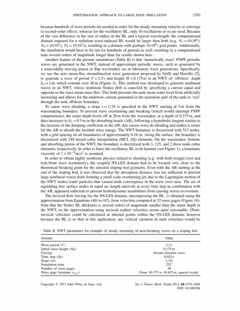
Another feature of the present simulations (Table II) is that ‘numerically exact’ FNPF periodicwaves are generated in the NWT, instead of approximate periodic waves, such as generated bya sinusoidally moving piston or flap wavemaker (as in laboratory wave generation). Specifically,we use the zero mean-flux streamfunction wave generation proposed by Grilli and Horrillo [5],to generate a wave of period T =2.5s and height H =0.175m in an NWT of ‘offshore’ depthho=1m, which extends over 40m (Figure 2). This method was developed to generate nonlinearwaves in an NWT, whose nonlinear Stokes drift is canceled by specifying a current equal andopposite to the wave mean mass flux. This both prevents the tank mean water level from artificiallyincreasing and allows for the undertow current generated in the nearshore part of the tank to ‘exit’through the tank offshore boundary.

To cause wave shoaling, a slope s=1/24 is specified in the NWT starting at 5m from thewavemaking boundary. To prevent wave overturning and breaking (which would interrupt FNPFcomputations), the water depth levels off at 20m from the wavemaker, at a depth of 0.375m, andthen increases to h1=0.5m in the absorbing beach (AB), following a hyperbolic tangent similar tothe increase of the damping coefficient in the AB; this causes wave de-shoaling and makes it easierfor the AB to absorb the incident wave energy. The NWT boundary is discretized with 513 nodes,with a grid spacing on all boundaries of approximately 0.16 m. Along the surface, the boundary isdiscretized with 249 mixed cubic interpolation (MCI, [4]) elements. On the wavemaker, bottom,and absorbing piston of the NWT, the boundary is discretized with 3, 125, and 2 three-node cubicelements, respectively. In order to force the oscillatory BL to be laminar (see Figure 1), a kinematicviscosity of 1×10−5m/s2 is assumed.

In order to obtain highly nonlinear physics related to shoaling (e.g. with both trough/crest andrear/front wave asymmetry), the coupled NS-LES domain had to be located very close to thetheoretical breaking point for the selected sloping bed geometry. Even with the AB starting at theend of the sloping bed, it was observed that the absorption distance was not sufficient to preventlarge nonlinear waves from forming a small scale overturning jet, due to the Lagrangian motion ofthe NWT nodes/water particles that caused node convergence in the wave crest area. The act ofregridding free surface nodes at equal arc length intervals at every time step in combination withthe AB, appeared sufficient to prevent hydrodynamic instabilities from causing waves to overturn.

The inviscid flow forcing for the NS-LES domain, encompassing the BL, is obtained using theapproximation from Equations (40) to (42), from velocities computed at 32 wave gages (Figure 10).Note that the Stokes BL thickness is several orders of magnitude smaller than the water depth inthe NWT, so the approximation using inviscid seabed velocities seems quite reasonable. [Note,inviscid velocities could be calculated at internal points within the NS-LES domain; howeverbecause the BL is so thin in this application, any vertical variation in such velocities would be

Table II. NWT parameters for example of steady streaming of near-breaking waves on a sloping bed.

Domain Value

Wave period (T ) 2.5 sInitial wave height (H0) 0.175mForcing Stream function waveTime step (!t) 0.025 sSlope (m) 1/24Simulation time 25TNumber of wave gages 38Wave gage locations (xg1) From 10.375 to 19.625m, spaced evenly




more likely caused by numerical errors than any physical variation; similarly, the velocity gradientis computed with finite differences but this could be made more accurate using the NWT boundaryintegral equation.]

The inviscid forcing is ramp-up by running the NWT for an initial 25 wave periods, and isthen used to force the NS solver. To do so, the final wave period of NWT simulations is repeatedfrom then on, to provide a quasi-periodic forcing. This assumes that the NWT has reached aquasi-periodic state by then, which is demonstrated, e.g. in Figure 11.

For each test, we use a moderately coarse NS grid of 32×32 (L×H ) points, with 100 timesteps per period (Table III). The NS domain is 8m long (from 11 to 19m from the wavemaker;Figure 11), 4.5 cm thick, and the simulations are run for 1000 wave periods. [The domain wasspecified with two points in the lateral direction, with a width of 10 cm, although this is presumedto be unimportant for this laminar case.] In general, a streaming velocity away from the beachwas observed (Figure 12), with significant variation across the domain. Interestingly, the trend of

0 12.5 25 37.5 50 62.5

0 12.5 25 37.5 50 62.5

0 12.5 25 37.5 50 62.5(s)

Figure 10. Example of surface elevation, and horizontal/vertical velocity componentssimulated at the NWT seabed (—), 15m from the wavemaker (averaging the results at

adjacent wave gages at 14.875 and 15.125m).

Figure 11. Free surface elevation predicted by NWT around the area of interest (from 11 to 19m fromthe wavemaker, with overlapping data from 5 to 21T every two periods. [Vertical exaggeration is 2x .]

The NS-LES domain is sketched for information.




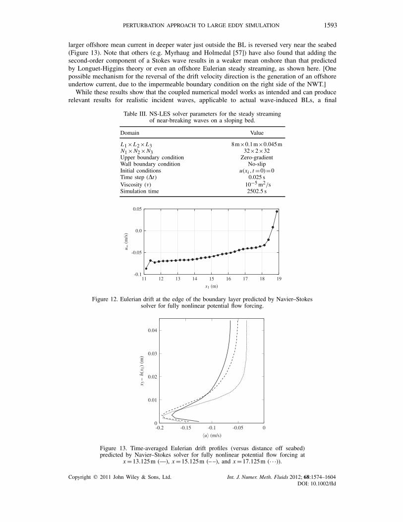
larger offshore mean current in deeper water just outside the BL is reversed very near the seabed(Figure 13). Note that others (e.g. Myrhaug and Holmedal [57]) have also found that adding thesecond-order component of a Stokes wave results in a weaker mean onshore than that predictedby Longuet-Higgins theory or even an offshore Eulerian steady streaming, as shown here. [Onepossible mechanism for the reversal of the drift velocity direction is the generation of an offshoreundertow current, due to the impermeable boundary condition on the right side of the NWT.]

While these results show that the coupled numerical model works as intended and can producerelevant results for realistic incident waves, applicable to actual wave-induced BLs, a final

Table III. NS-LES solver parameters for the steady streamingof near-breaking waves on a sloping bed.

Domain Value

L1×L2×L3 8m×0.1m×0.045mN1×N2×N3 32×2×32Upper boundary condition Zero-gradientWall boundary condition No-slipInitial conditions u(xi , t=0)=0Time step (!t) 0.025 sViscosity ($) 10−5m2/sSimulation time 2502.5 s

11 12 13 14 15 16 17 18 19-0.1

-0.05

0.0

0.05

x1 (m)

u ∞(m

/s)

Figure 12. Eulerian drift at the edge of the boundary layer predicted by Navier–Stokessolver for fully nonlinear potential flow forcing.

-0.2 -0.15 -0.1 -0.05 00

0.01

0.02

0.03

0.04

u (m/s)

x 3−h(x 1)(m

)

Figure 13. Time-averaged Eulerian drift profiles (versus distance off seabed)predicted by Navier–Stokes solver for fully nonlinear potential flow forcing at

x=13.125m (—), x=15.125m (– –), and x=17.125m (· · ·)).




demonstration is required to show that the SGS models implemented in the LES are adequate toreproduce the desired turbulent flow properties. This is done in the following section.

4.2. Turbulent oscillatory boundary layers

We next validate the LES for turbulent oscillatory BLs. We choose a uniform oscillatory flowbecause of the lack of sufficiently detailed experimental data for more complex wave-induced flows.To compare results with the laboratory experiments of Jensen et al’s [43], which were performedin an oscillatory flume (U-tube), the model inviscid forcing was selected similarly to the initiallaminar BL test cases, as a vertically uniform oscillatory flow (see Equation (43)), with velocityamplitude Uo and period T (#=2)/T ). Jensen et al.’s experiments consisted in 15 different testcases, of which we selected for comparison two cases with a rough bed: nos. 12 and 13 (seephysical data in Table IV). In each case, the mean velocity and Reynolds stresses were measuredas a function of time and elevation over the rough bed in the BL.

To achieve good accuracy and resolution in simulated results and also to ensure that the numberof ‘samples’ used for ensemble averaging is large enough, a NS grid size of 128×32×64 is used insimulations (see numerical parameters in Table V), slightly larger than that used by Radhakrishnanand Piomelli [27] who recently reported on similar comparisons. Note, for very simple flows suchas considered here, this need for performing averaging operations is one disadvantage of NS-LESmodels as compared with an RANS model, which directly compute mean quantities.

4.2.1. Wall stress and mean velocity. Jensen et al. did not measure wall stress 〈&w〉, but rather(for test #13 only) they did measure a time-series of the mean streamwise velocity at a very smallheight over the wall, x3=0.0006 A (relative to the amplitude of oscillation A=U0/#; equivalentto a height x3 of 1.86mm), which we used together with a log-law assumption, to predict wallstress. Figures 14 and 15 show wall stress computed for tests #12 and #13, using the three SGS

Table IV. Parameters (period T , free-stream maximum velocity U0, viscosity $, Nikuradse roughness ks ,and free-stream amplitude A) for selected laboratory experiments of turbulent oscillatory BLs [43] used

for comparison with numerical simulations.

Test T U0 $ ksno. (s) (m/s) (m2/s) Re (mm) A/ks

12 9.72 1.02 1.14×10−6 1.6×106 0.84 180013 9.72 2.00 1.14×10−6 6.0×106 0.84 3700

Table V. Parameters for numerical simulations of turbulent oscillatory BLs.

Domain Value

L1×L2×L3 636.3"S×318.2"S×100"SN1×N2×N3 128×64×32Grid discretization (Smagorinsky SGS model) Uniform grid spacingGrid discretization (dynamic SGS models) Vertical exponential stretching with ratio 1.1

Minimum grid height: 0.93mmAspect ratio at wall: 10:1:10

Upper boundary condition Zero-gradientWall boundary condition Log-layer approximationWall roughness z0=2.8×10−5 mInitial conditions u(xi , t=0)=0Simulation spin-up time 5TForcing uI1(t)=U0 sin#t!t T/4860 (test 12) or T/9720 (test 13)Simulation time 10TOutput sampling frequency Every T/12




models in the NS-LES; in the latter test, this is compared with experimental values inferred fromnear-wall velocity measurements.

Wall stress is qualitatively consistent among the three SGS turbulence models used. Additionally,for test #13, numerical results with the DSM and DMM approaches agree well both with eachother and with experiments, while these are underpredicted by the Smagorinsky model; a betteragreement for the latter could probably be achieved by calibrating the Smagorinsky coefficient.Note that while of the DSM and DMM approaches show a good performance, they rely on theenhanced eddy viscosity near the wall, which tends towards the mixing-length approximation.A time-invariant eddy viscosity distribution proportional to the height above the wall was foundby Grant and Madsen [31] to produce good results for both wall stress and mean flow, thus it isreasonable to expect that the DSM and DMM approaches would also be successful.

The results in Figures 16 and 17 show that model results for the mean flow velocity, 〈u1〉, areagain qualitatively consistent among the three SGS turbulence models used, with the Smagorinskyapproach underestimating the BL thickness. Numerical results using DSM or DMM agree wellwith experiments, for both the #12 and 13 test cases, at six selected phases of the flow, over halfa period of oscillation.

4.2.2. Turbulent intensity and Reynolds stress. For both test cases #12 and 13, we calculated thestreamwise turbulent intensity 〈u′2

1 〉1/2 (Figures 18 and 19), the vertical (wall normal) turbulentintensity 〈u′2

3 〉1/2 (Figures 20 and 21), and the Reynolds stresses 〈u′1u

′3〉 (Figures 22 and 23), and

compared those to experiments. The figures show a good agreement of all model results withexperiments when using DSM or DMM, but not so with the Smagorinsky model. In particular, fortest #12, at the lower Reynolds number, the Smagorinsky approach fails to produce much resolvedturbulence. This highlights the significance of having to tune this model’s coefficient to differentflow conditions.

Near the wall, all simulation results underpredict the experimental turbulence intensity. Forthe constant coefficient Smagorinsky model, this is expected because this model is known to

Figure 14. Numerical simulations of turbulent oscillatory BL: mean wall stress, 〈&w〉 (determined bylog-law) as a function of phase angle for conditions of test #12 [43] with different SGS models: (—)

Smagorinsky; (– –) dynamic Smagorinsky; and (· · ·) DMM.

Figure 15. Same case as Figure 14, for test #13, with comparison to experiments (•).




Figure 16. Same case as Figure 14. Mean streamwise velocity profiles, 〈u1〉, for test #12.

Figure 17. Same case as Figure 14. Mean streamwise velocity profiles, 〈u1〉, for test #13.

overpredict near-wall dissipation. For the dynamic models, the underpredicted turbulent intensityis more likely due to the grid aspect ratio near the wall. The vertical stretching of the grid results in‘pancake’-like grid cells, which are significantly wider in the streamwise and spanwise directionsthan in the wall-normal direction. The typical eddy size, however, is of similar size in all directions,and so the implicit grid-scale filter averages over many eddies in a way similar to a RANS ensembleaverage. The most similar numerical study to the present one is the LES work of Radhakrishnanand Piomelli [27], which studied test case #13. Their results for the near-wall turbulent intensityare similar to ours for most phases of the oscillation, although Radhakrishnan and Piomelli didobtain a better agreement with experiments at #t=60◦ and #t=90◦, albeit using different SGSmodels, and without having the large aspect ratio for the grid cells near the wall.

Far from the wall, there is an occasional underprediction of the turbulent intensity. Othernumerical studies have reported this problem as well, whichMellor [39] suggests is an experimentalartifact. The amplitude of the oscillation for test #13 is 3.1m, so a fluid particle can move as faras 6.2m over the course of each oscillation. Hence, at the end of each period (i.e. around 0◦),some of the fluid being measured may have a half-period earlier been outside of the 10 m straight




Figure 18. Streamwise turbulent intensity, 〈u′21 〉1/2, for test #12.

0 0.05 0.10

20

40

60

80

100

x 3/δ

S

ωt = 0o

0 0.05 0.1

ωt = 30o

0 0.05 0.1

ωt = 60o

0 0.05 0.10

20

40

60

80

100

x 3/δ

S

ωt = 90o

0 0.05 0.1

u 21

1/ 2/U0

ωt = 120o

0 0.05 0.1

ωt = 150o

Figure 19. Streamwise turbulent intensity, 〈u′21 〉1/2, for test #13.

test section of the oscillatory water tunnel used in experiments. Although Jensen et al. took someadditional measurements to attempt to show that this would have no effect, it does seem to explainthe outlier seen at the 0◦ phase angle (e.g. Figure 18). The results far from the wall are similarto others (e.g. Radhakrishnan and Piomelli), although our turbulent intensities match experimentsomewhat better far from the wall at phases 0◦ and 30◦.

In some cases, the size of the discretization may prove to be the limiting factor. For case #13,for instance, the Reynolds stress at 90◦ was experimentally measured to be maximum at 2.6"S overthe bed (Figure 23), whereas the first grid cell is 3 "S high. Important physics may not be properlymodeled as a result. Note that Sleath [48] found that the Reynolds stress is a minor contributor tothe shear stress. As a result, one would expect that the vertical momentum flux would be governedmore by the periodic velocity components than the turbulent momentum flux, and thus more studywould be required to verify whether resolving this peak in Reynolds stress is important for thenumerical simulations.




Figure 20. Wall normal turbulent intensity, 〈u′23 〉1/2, for test #12.

Figure 21. Wall normal turbulent intensity, 〈u′23 〉1/2, for test #13.

4.2.3. Velocity spectra. In addition to examining second-order turbulence statistics, we analyzedvelocity spectra, such as the streamwise velocity fluctuation spectrum, which can be defined asthe discrete Fourier transform:

E11(k1)=∣∣∣∣∣Ni∑n=1

[u1]n, j,ke−2)inkx /Ni

∣∣∣∣∣ (51)

and can also be phase-averaged. Note, such spectra are computed directly from the resolvedvelocities at each grid point, and thus develop as a result of simulations. It should be stressed thatthe numerical method is not a spectral method and, hence, spectra are not a priori assumed in theSGS models used here.

Figure 24, for instance, shows the phase-averaged spatial velocity power spectra for the DSMtest #13 run at 0◦. We are able to see at least what appears to be the inertial subrange in thespectral results (slope 5/3). Note that the spectra are not smooth lines, but somewhat stochastic.This indicates that the scale of the largest vortex structures is not well resolved, which is some-what expected because particles in the free-stream oscillate horizontally over 2A=2U0/#≈6.2m,




Figure 22. Reynolds stress, 〈u′1u

′3〉, for test #12.

Figure 23. Reynolds stress, 〈u′1u

′3〉, for test #13.

whereas the computational domain is approximately an eighth of that size. A similar problem wasencountered by Costamagna et al. [88], but because the Jensen et al. data is for fully turbulentconditions, we may use phase-averaging (i.e. averaging the data for the same phase from differentoscillations) in order to smooth results, as we have done above. Because the dynamics is mostlycontrolled by the near-wall behavior (where the eddies are smaller), the largest scales are unlikelyto be particularly important, but future studies should consider using larger computational domainsto verify this claim.

4.2.4. Two-point spatial correlation. One premise of the modeling of turbulent flows in ‘infinitelylong’ oscillatory BLs, using a finite length spatially periodic domain, is that there is no correlationbetween the velocity fluctuations a half-domain away (see, e.g. [1]). This will be achieved providedthe domain size is large enough, which can be a posteriori verified in numerical results by calculatingand verifying that the two-point spatial autocorrelation of the perturbation velocity field is nearlyzero, between points half a domain away in the horizontal direction.

Figure 25 shows the autocorrelation of each of the three components of the velocity fluctuationsin both the streamwise and spanwise directions at a given height for the DSM run of test 13. The




Figure 24. Non-dimensional velocity spectra for the resolved streamwise velocity field.

Figure 25. Two-point spatial autocorrelation functions for the component velocity fluctuations, u′1 (—),

u′2 (– –), u′

3 (· · ·), at the first gridpoint above the rough bed, as a function of distance for test case #13, inboth the streamwise direction (averaged over the spanwise direction; upper panel) and spanwise direction

(averaged over the streamwise direction; lower panel).

autocorrelation function is very small for much of the domain, in both streamwise and spanwisedirections, indicating that the domain is large enough.

5. CONCLUSIONS

A perturbation approach to the NS equations was developed for simulating wave-induced BL flows,in a coupled model implementation, in which the NS domain is embedded within a fully nonlinearinviscid NWT. The NS equations are solved using an LES with a variety of SGS turbulencemodels. For many coastal engineering problems, the physics of waves is such that the flow is




nearly irrotational in most of the fluid domain, except for thin free surface and bottom BLs. Hence,the region of the seafloor requiring full NS modeling may be relatively small, which justifies thecoupled/hybrid approach and allows using efficient and relevant models for various parts or regionsof the solution, based on the corresponding salient physics. Another advantage of the perturbationmethod is that the inviscid component of the flow fields (which is either analytical or obtained inthe NWT) is not subject to the numerical errors of the NS solver.

The NS solver is first validated for simple laminar or turbulent oscillatory BL flows (for theformer, the eddy viscosity was zero and the LES was bypassed). For laminar cases, the results arevery close to theoretical closed-form solutions for oscillatory BLs, both in simple periodic flows orunder linear wave forcing. Moreover, simulations demonstrate the expected rates of convergenceto the exact solution, with both spatial and temporal discretizations. The hybrid NWT-NS model isthen used to compute the steady streaming current due to fully nonlinear periodic waves, shoalingon a slope near the breaking point, which demonstrates the possibilities of the approach to simulaterealistic nearshore wave processes. Simulations for rough turbulent oscillatory BL flows are finallyperformed, which favorably compared with experimental data, for both mean and turbulent fields.

More specifically, the results for 1D (i.e. forced by spatially uniform horizontal flows) laminaroscillatory BLs over a flat boundary showed the expected second-order convergence of numericalerrors to the Stokes solution [86], in both space and time. This was to be expected from thepublished results, as all the modified terms in the new perturbed NS equations, as compared withthe original Cui and Street work [22], were zero for this very simple test case. Similarly, goodresults were obtained for laminar oscillatory BLs induced by linear Stokes waves, which yieldnon-spatially uniform forcing flows. This case further tested the application of the inviscid forcingterms in the perturbation form of the momentum equations (i.e. nonlinear convective terms). Inthese simulations, we first used spatially periodic boundary conditions in both lateral directions ofthe NS domain and found that the computed steady streaming velocities in the BL closely matchedthose theoretically predicted by Longuet-Higgins [50]. Effects of using more general (gradientfree) open boundary conditions were then tested in the case of wave forcing, and results wereshown to be accurate within half a wavelength of the lateral boundaries of the NS domain.

Preliminary numerical tests of the fully coupled NWT-NS model were performed, for simple‘numerically exact’ nonlinear periodic incident waves shoaling over a 1:24 slope. Specifically, wecalculated fully nonlinear inviscid flow fields near the breaking point in the NWT, for periodicwaves shoaling over a plane slope, and used those to force BL flows (limited to laminar cases)in a small embedded near-bottom NS-LES domain. Results show that for the selected parameters,unlike with the flat-bottom linear wave forcing case, the steady streaming in the BL is both strongerand directed offshore, with significant spatial variation.

Finally, for rough turbulent oscillatory BL flows, the LES model, with various SGS, was ableto accurately predict measured mean flow fields, wall stress, and second-order turbulent statistics.Specifically, all results favorably compared with the experimental data of Jensen et al.’s test #12and 13 [43] (except over small regions for the turbulent fields). Our simulations with dynamicSGS showed somewhat better agreement with the measured turbulent intensity far from the wallthan the recent results of Radhakrishnan and Piomelli [27]. This may be partly due to using agradient-free boundary condition, as opposed to setting the wall-normal velocity to zero in thefree-stream, and to increased model accuracy when using the perturbation method.

While these experiments show that a hybrid NWT-LES can accurately determine turbulentcharacteristics of coastal flows, note that for turbulent BLs over complex 3D bathymetry, thistechnique may still be computationally demanding depending on the size of the domain. A LESof turbulent flow needs to simulate eddies which may be several orders of magnitude smallerthan the size of the domain, in 3D (regardless of whether the driving force is uniform, or variesin one or more dimensions), and perhaps over several hundreds of wave periods to determinee.g. the induced steady streaming velocity. Limitations have existed for high-Reynolds laboratorymeasurements as well, however, and only recently has the wave-induced steady streaming velocityof a fully turbulent BL over sloping bed been made [89]. More complex applications should bemade possible as computer performance increases.




In future work, we will build on the model capabilities demonstrated in these initial somewhatidealized numerical applications, by simulating more general wave-induced turbulent BL flows.We will finally add a sub-model for sediment suspension and transport, with the eventual goal ofbeing able to simulate wave-induced bed form development around objects on the seabed.

ACKNOWLEDGEMENTS

Both authors gratefully acknowledge support of grant Nb. N000140510068 from the US Office of NavalResearch (ONR) Coastal Geosciences Division (code 321CG). In addition, the first author acknowledgessupport from an ONR-NDSEG fellowship. Prof. R. Street and Prof. O. Fringer are thanked for providingthe initial LES code, and Dr Senthil Radhakrishnan is gratefully acknowledged for providing us with acopy of the Jensen et al. data.

REFERENCES

1. Moin P, Mahesh K. Direct numerical simulation: a tool in turbulence research. Annual Review of Fluid Mechanics1998; 30:539–578.

2. Deardorff JW. A numerical study of three-dimensional turbulent channel flow at large Reynolds numbers. Journalof Fluid Mechanics 1970; 41(2):453–480.

3. Zang Y, Street RL, Koseff J. A non-staggered grid, fractional step method for the time-dependent incompressibleNavier–Stokes equations in curvilinear coordinates. Journal of Computational Physics 1994; 114(1):18–33.

4. Grilli ST, Subramanya R. Numerical modeling of wave breaking induced by fixed or moving boundaries.Computational Mechanics 1996; 17:374–391.

5. Grilli ST, Horrillo J. Numerical generation and absorption of fully nonlinear periodic waves. Journal of EngineeringMechanics 1997; 123(10):1060–1069.

6. Grilli ST, Voropayev S, Testik FY, Fernando HJS. Numerical modeling and experiments of wave shoaling overburied cylinders in sandy bottom. Proceedings of the 13th Offshore and Polar Engineering Conference, Honolulu,HI, 2003; 405–412.

7. Wei G, Kirby JT. A time-dependent numerical code for extended Boussinesq equations. Journal of Waterway,Port, Coastal, and Ocean Engineering 1995; 120:251–261.

8. Wei G, Kirby JT, Grilli ST, Subramanya R. A fully nonlinear Boussinesq model for surface waves. I. Highlynonlinear, unsteady waves. Journal of Fluid Mechanics 1995; 294:71–92.

9. Grilli ST. On the development and application of hybrid numerical models in nonlinear free surface hydrodynamics.In Proceedings of the Eighth International Conference on Hydrodynamics, Nantes, France, Ferrant P, Chen XB(eds). 2008; 21–50.

10. Guignard S, Grilli ST, Marcer R, Rey V. Computation of shoaling and breaking waves in nearshore areas by thecoupling of BEM and VOF methods. Proceedings of the 9th Offshore and Polar Engineering Conference, vol.3. Brest, France, 1999; 304–309.

11. Lachaume C, Biausser B, Grilli ST, Fraunie P, Guignard S. Modeling of breaking and post-breaking waveson slopes by coupling of BEM and VOF methods. Proceedings of the 13th Offshore and Polar EngineeringConference, Honolulu, HI, 2003; 353–359.

12. Biausser B, Grilli ST, Fraunie P, Marcer R. Numerical analysis of the internal kinematics and dynamics ofthree-dimensional breaking waves on slopes. International Journal of Offshore and Polar Engineering 2004;14(4):247–256.

13. Corte C, Grilli ST. Numerical modeling of extreme wave slamming on cylindrical offshore support structures.Proceedings of the 16th Offshore and Polar Engineering Conference, San Francisco, CA, U.S.A., vol. 3, 2006;394–401.

14. Gilbert RW, Zedler EA, Grilli ST, Street RL. Progress on nonlinear-wave-forced sediment transport simulation.IEEE Journal of Oceanic Engineering 2007; 32(1):236–248.

15. Zang Y. On the development of tools for the simulation of geophysical flows. Ph.D. Thesis, Stanford University,1993.

16. Zang Y, Street RL. Numerical simulation of coastal upwelling and interfacial instability of a rotating and stratifiedfluid. Journal of Fluid Mechanics 1995; 305:47–75.

17. Fringer OB, Street RL. The dynamics of breaking progressive interfacial waves. Journal of Fluid Mechanics2003; 494:319–353.

18. Zedler EA, Street RL. Large-eddy simulation of sediment transport: currents over ripples. Journal of HydraulicEngineering 2001; 127(6):444–452.

19. Zedler EA, Street RL. Large-eddy simulation of sediment transport: currents over ripples. Journal of HydraulicEngineering 2006; 132(2):180–193.

20. Kim K, Sirviente AI, Beck RF. The complementary RANS equations for the simulation of viscous flows.International Journal for Numerical Methods in Fluids 2005; 48:199–229.

21. Alessandrini B. Thèse d’habilitation en vue de diriger les recherches. Ph.D. Thesis, Ecole Centrale de Nantes,2007.




22. Cui A, Street RL. Large-eddy simulation of turbulent rotating convective flow development. Journal of FluidMechanics 2001; 447:53–84.

23. Grilli ST, Harris JC, Greene N. Modeling of wave-induced sediment transport around obstacles. Proceedingsof the 31st Coastal Engineering Conference. World Scientific Publishing Company: Hamburg, Germany, 2009;1638–1650.

24. Chou YJ, Fringer OB. Modeling dilute sediment suspension using large-eddy simulation with a dynamic mixedmodel. Physics of Fluids 2008; 20:115103.1–115103.13.

25. Chou YJ, Fringer OB. Consistent discretization for simulations of flows with moving generalized curvilinearcoordinates. International Journal for Numerical Methods in Fluids 2009; 62:802–826.

26. Salon S, Armenio V, Crise A. A numerical investigation of the Stokes boundary layer in the turbulent regime.Journal of Fluid Mechanics 2007; 570:253–296.

27. Radhakrishnan S, Piomelli U. Large-eddy simulation of oscillating boundary layers: model comparison andvalidation. Journal of Geophysical Research 2008; 113(C02022):14.

28. Grilli ST, Guyenne P, Dias F. A fully nonlinear model for three-dimensional overturning waves over arbitrarybottom. International Journal for Numerical Methods in Fluids 2001; 35(7):829–867.

29. Dean RG, Dalrymple RA. Water Wave Mechanics for Engineers and Scientists, Advanced Series on OceanEngineering, vol. 2. World Scientific Publishing Company: Singapore, 1991.

30. Kajiura K. A model for the bottom boundary layer in water waves. Journal of Fluid Mechanics 1968; 182:369–409.31. Grant WD, Madsen OS. Combined wave and current interaction with a rough bottom. Journal of Geophysical

Research 1979; 84(C4):1797–1808.32. Trowbridge JH, Madsen OS. Turbulent wave boundary layers: 1. Model formulation and first order solution.

Journal of Geophysical Research 1984; 89(C5):7989–7997.33. Davies AG. A model of oscillatory rough turbulent boundary flow. Estuarine, Coastal and Shelf Science 1986;

23(3):353–374.34. Blondeaux P. Turbulent boundary layer at the bottom of gravity waves. Journal of Hydraulic Research 1987;

25:447–464.35. Aydin I, Shuto N. An application of the k−! model to oscillatory boundary layers. Coastal Engineering in Japan

1988; 30(2):11–24.36. Justesen P. Prediction of turbulent oscillatory flow over rough beds. Coastal Engineering 1988; 12:257–284.37. Justesen P. A note on turbulence calculations in the wave boundary layer. Journal of Hydraulic Research 1991;

29:699–711.38. Thais L, Chapalain G, Smaoui H. Reynolds number variation in oscillatory boundary layers. Part I. Purely

oscillatory motion. Coastal Engineering 1999; 36:111–146.39. Mellor G. Oscillatory bottom boundary layers. Journal of Physical Oceanography 2002; 32(11):3075–3088.40. Tanaka SH, Sana A. Characteristics of turbulent boundary layers over a rough bed under saw-tooth waves and

its application to sediment transport. Coastal Engineering 2008; 55(12):1102–1112.41. Kamphuis JW. Friction factor under oscillatory waves. Journal of Waterways, Harbors Coastal Engineering

Division (ASCE) 1975; 101:135–144.42. Sleath JFA. Velocity measurements close to the bed in a wave tank. Journal of Fluid Mechanics 1970; 42:111–123.43. Jensen BL, Sumer BM, Fredsoe J. Turbulent oscillatory boundary layers at high Reynolds numbers. Journal of

Fluid Mechanics 1989; 206:265–297.44. Jonsson IG, Carlsen NA. Experimental and theoretical investigations in an oscillatory turbulent boundary layer.

Journal of Hydraulic Research 1976; 14(1):45–60.45. Sleath JFA. Transition in turbulent oscillatory flow over rough beds. Journal of Waterways, Harbors Coastal

Engineering Division (ASCE) 1988; 114:18–33.46. Hino M, Kashiwanayagi M, Nakayami A, Hara T. Experiments on the turbulence statistics and the structure of

a reciprocating oscillatory flow. Journal of Fluid Mechanics 1983; 131:363–400.47. Pope SB. Turbulent Flows. Cambridge University Press: Cambridge, 2000.48. Sleath JFA. Turbulent oscillatory flow over rough beds. Journal of Fluid Mechanics 1987; 182:369–409.49. Longuet-Higgins MS. Mass transport in water waves. Philosophical Transactions of the Royal Society of London

A 1953; 245:535–581.50. Longuet-Higgins MS. The mechanics of the boundary layer near the bottom in a progressive wave. Proceedings

of the Sixth International Conference on Coastal Engineering, Gainesville, FL, U.S.A., 1958; 184–193.51. Johns B. Residual flow and boundary shear stress in the turbulent bottom layer beneath waves. Journal of

Physical Oceanography 1977; 7:733–738.52. Jacobs SJ. Mass transport in a turbulent boundary layer under a progressive water wave. Journal of Fluid

Mechanics 1984; 146:303–312.53. Hsu TW, Ou SH. On the mass transport of water waves in a turbulent boundary layer. Ocean Engineering 1994;

21(2):195–206.54. Chowdhury AC, Sato M, Ueno A. Numerical model of the turbulent wave boundary layer induced by finite

amplitude water waves. Applied Ocean Research 1997; 19:201–209.55. Deigaard R, Jacobsen JB, Fredsøe J. Net sediment transport under wave groups and bound long waves. Journal

of Geophysical Research 1999; 104(C6):13559–13575.56. Davies AG, Villaret C. Eulerian drift induced by progressive waves above rippled and very rough beds. Journal

of Geophysical Research 1999; 104(C1):1465–1488.




57. Myrhaug D, Holmedal LE. Bottom friction caused by boundary layer streaming beneath random waves forlaminar and smooth turbulent flow. Ocean Engineering 2005; 32(2):195–222.

58. Scandura P. Steady streaming in a turbulent oscillating boundary layer. Journal of Fluid Mechanics 2007;571:265–280.

59. Holmedal LE, Myrhaug D. Wave-induced steady streaming, mass transport and net sediment transport in roughturbulent ocean bottom boundary layers. Continental Shelf Research 2009; 29:911–926.

60. Mei CC. The Applied Dynamics of Ocean Surface Waves (2nd edn), Advanced Series on Ocean Engineering.World Scientific Publishing Company: Singapore, 1989.

61. Longuet-Higgins MS, Cokelet ED. The deformation of steep surface waves on water. I. A numerical method ofcomputation. Proceedings of the Royal Society of London. Series A, Mathematical and Physical Sciences 1976;350(1660):1–26.

62. Russell RCH, Osorio JDC. An experimental investigation of drift profiles in a closed channel. Proceedings ofthe 6th Coastal Engineering Conference, Gainesville, FL, U.S.A., 1958; 171–193.

63. Collins JI. Inception of turbulence at the bed under periodic gravity waves. Journal of Geophysical Research1963; 68(21):6007–6014.

64. Johns B. On the mass transport induced by oscillatory flow in a turbulent boundary layer. Journal of FluidMechanics 1970; 43:177–185.

65. Brebner A, Askew JA, Law SW. The effect of roughness on the mass-transport of progressive gravity waves.Proceedings of the 10th Coastal Engineering Conference, Tokyo, Japan, 1966; 175–184.

66. Bijker EW, Kalkwijk JPT, Pieters T. Mass transport in gravity waves on a sloping bottom. Proceedings of the14th Coastal Engineering Conference, Copenhagen, Denmark, 1974; 24–28.

67. van Doorn T. Experimental investigation of near-bottom velocities in water waves without and with a current.Technical Report, Delft Hydraulics Laboratory, 1981.

68. Ribberink JS, Al-Salem AA. Sheet flow and suspension of sand in oscillatory boundary layers. Coastal Engineering1995; 25:205–255.

69. Marin F. Eddy viscosity and Eulerian drift over rippled beds in waves. Coastal Engineering 2004; 50(3):139–159.70. Leonard BP. A stable and accurate convective modeling procedure based on quadratic upstream interpolation.

Computer Methods in Applied Mechanics and Engineering 1979; 19:59–98.71. Moeng CH. A large-eddy simulation model for the study of planetary boundary-layer turbulence. Journal of

Atmospheric Science 1984; 46:2311–2330.72. Cabot W, Moin P. Approximate wall boundary conditions in the large-eddy simulation of high Reynolds number

flows. Flow, Turbulence, and Combustion 1999; 63:269–271.73. Piomelli U, Balaras E. Wall-layer models for large-eddy simulation. Annual Review of Fluid Mechanics 2002;

34:349–374.74. Nakayama A, Noda H, Maeda K. Similarity of instantaneous and filtered velocity fields in the near wall region

of zero-pressure gradient boundary layer. Fluid Dynamics Research 2004; 35:299–321.75. Smagorinsky J. General circulation experiments with the primitive equations, I. The basic experiment. Monthly

Weather Review 1963; 91:99–164.76. Lilly DK. Representation of small scale turbulence in numerical simulation experiments. IBM Scientific Computing

Symposium on Environmental Sciences, Yorktown Heights, New York, U.S.A., 1967; 195–210.77. Germano M, Piomelli U, Moin P, Cabot WH. A dynamic subgrid-scale eddy viscosity model. Physics of Fluids

A 1991; 3(7):1760–1765.78. Lilly DK. A proposed modification of the Germano subgrid-scale closure method. Physics of Fluids A 1992;

4(3):633–635.79. Germano M. Turbulence: the filtering approach. Journal of Fluid Mechanics 1992; 238:325–336.80. Lund TS. On the use of discrete filters for large eddy simulation. Technical Report, Annual Research Briefs,

Center for Turbulence Research, 1997.81. Germano M. A proposal for a redefinition of the turbulent stresses in the filtered Navier–Stokes equations. Physics

of Fluids 1986; 29:2323–2324.82. Vasilyev OV, Lund TS, Moin P. A general class of commutative filters for LES in complex geometries. Journal

of Computational Physics 1998; 146:82–104.83. Chow FK, Street RL. Explicit filtering and reconstruction turbulence modeling for large-eddy simulation of

field-scale flows. Advances in Hydro-science and Engineering 2004; 6:1–12.84. Chow FK, Street RL, Xue M, Ferziger JH. Explicit filtering and reconstruction turbulence modeling for large-eddy

simulation of neutral boundary layer flow. Journal of the Atmospheric Sciences 2005; 62:2058–2077.85. Piomelli U, Balaras E, Pasinato H, Squires KD, Spalart PR. The inner–outer layer interface in large-eddy

simulations with wall-layer models. International Journal of Heat and Fluid Flow 2003; 24:538–550.86. Stokes GG. On the effect of the internal friction of fluids on the motion of pendulums. Cambridge Philosophical

Transactions 1851; 9:8–106.87. Nielsen P. Coastal Bottom Boundary Layers and Sediment Transport, Advanced Series on Ocean Engineering,

vol. 4. World Scientific Publishing Company: Singapore, 1992.88. Costamagna P, Vittori G, Blondeaux P. Coherent structures in oscillatory boundary layers. Journal of Fluid

Mechanics 2003; 474:1–33.89. Scandura P. Measurements of wave-induced steady currents outside the surf zone. HYDRALAB III Joint User

Meeting, Hannover, Germany, 2010.




aperturbationapproachtolargeeddysimulationofwave-induced

Documents