Aperture Photometry ToolAuthor(s): Russ R. Laher, Varoujan Gorjian, Luisa M. Rebull, Frank J. Masci, John W. Fowler,George Helou, Shrinivas R. Kulkarni and Nicholas M. LawReviewed work(s):Source: Publications of the Astronomical Society of the Pacific, Vol. 124, No. 917 (July 2012),pp. 737-763Published by: The University of Chicago Press on behalf of the Astronomical Society of the PacificStable URL: http://www.jstor.org/stable/10.1086/666883 .Accessed: 23/08/2012 14:48

Your use of the JSTOR archive indicates your acceptance of the Terms & Conditions of Use, available at .http://www.jstor.org/page/info/about/policies/terms.jsp

.JSTOR is a not-for-profit service that helps scholars, researchers, and students discover, use, and build upon a wide range ofcontent in a trusted digital archive. We use information technology and tools to increase productivity and facilitate new formsof scholarship. For more information about JSTOR, please contact support@jstor.org.

.

The University of Chicago Press and Astronomical Society of the Pacific are collaborating with JSTOR todigitize, preserve and extend access to Publications of the Astronomical Society of the Pacific.

http://www.jstor.org

Aperture Photometry Tool

RUSS R. LAHER,1 VAROUJAN GORJIAN,2 LUISA M. REBULL,3 FRANK J. MASCI,4 JOHN W. FOWLER,4

GEORGE HELOU,4 SHRINIVAS R. KULKARNI,5 AND NICHOLAS M. LAW6

Received 2010 March 29; accepted 2012 May 24; published 2012 July 10

ABSTRACT. Aperture Photometry Tool (APT) is software for astronomers and students interested in manuallyexploring the photometric qualities of astronomical images. It is a graphical user interface (GUI) designed to allowthe image data associated with aperture photometry calculations for point and extended sources to be visualized and,therefore, more effectively analyzed. The finely tuned layout of the GUI, along with judicious use of color-codingand alerting, is intended to give maximal user utility and convenience. Simply mouse-clicking on a source in thedisplayed image will instantly draw a circular or elliptical aperture and sky annulus around the source and willcompute the source intensity and its uncertainty, along with several commonly used measures of the local skybackground and its variability. The results are displayed and can be optionally saved to an aperture-photometry-table file and plotted on graphs in various ways using functions available in the software. APT is geared towardprocessing sources in a small number of images and is not suitable for bulk processing a large number of images,unlike other aperture photometry packages (e.g., SExtractor). However, APT does have a convenient source-list toolthat enables calculations for a large number of detections in a given image. The source-list tool can be run either inautomatic mode to generate an aperture photometry table quickly or in manual mode to permit inspection andadjustment of the calculation for each individual detection. APT displays a variety of useful graphs with justthe push of a button, including image histogram, x and y aperture slices, source scatter plot, sky scatter plot,sky histogram, radial profile, curve of growth, and aperture-photometry-table scatter plots and histograms. APThas many functions for customizing the calculations, including outlier rejection, pixel “picking” and “zapping,”and a selection of source and sky models. The radial-profile-interpolation source model, which is accessed viathe radial-profile-plot panel, allows recovery of source intensity from pixels with missing data and can be especiallybeneficial in crowded fields.

1. INTRODUCTION

Aperture photometry in astronomical image-data analysis isa basic technique for measuring the brightness of an astronom-ical object, such as a star or galaxy. It is the calculation of sourceintensity by summing the measured counts from a subimagecontaining the source (or possibly sources) and subtractingthe sky background contribution estimated from a nearby im-aged region that excludes the source of interest (Da Costa1992). The subimage containing the source brightness, orso-called aperture, is a bounding region for the calculation, a

two-dimensional area used to define just the portion of a photo-graph or digital image of the nighttime sky that contains most, ifnot nearly all, of the observed radiance of the astronomical ob-ject under investigation. Conventionally, the aperture is centeredon the source of interest, although the calculation is usually in-sensitive to exact aperture placement, and, in some cases, it isdesirable to offset the aperture slightly from the source’s centerto possibly omit the effect of a neighboring source. The shape ofthe aperture is circular in its simplest form. Often, the shape ofan astronomical object, such as a spiral galaxy viewed at an ob-lique angle, will determine the aperture shape that is optimal forits scientific study (e.g., elliptical). In addition to geometricalconsiderations, photometric criteria can govern the aperture’sshape (e.g., a set of contiguous pixels in a digital image withdata values greater than some threshold). A multiplier greaterthan one, called an aperture correction, is employed to correctfor source intensity outside of the aperture, which is needed forcases where source-crowding effects warrant using a smalleraperture. In theory, an aperture correction is always neededbecause of limited bandwidth considerations, but, in practice,no aperture correction is made for sufficiently large apertures.As the size of an aperture is increased, the signal from the source

1Spitzer Science Center, California Institute of Technology, Mail Stop 314-6,Pasadena, CA 91125; laher@ipac.caltech.edu.

2Jet Propulsion Laboratory, California Institute of Technology, Mail Stop 169-506, Pasadena, CA 91109.

3Spitzer Science Center, California Institute of Technology, Mail Stop 220-6,Pasadena, CA 91125.

4 Infrared Processing and Analysis Center, California Institute of Technology,Mail Stop 100-22, Pasadena, CA 91125.

5Caltech Optical Observatories, California Institute of Technology, Mail Stop249-17, Pasadena, CA 91125.

6 Dunlap Institute for Astronomy and Astrophysics, University of Toronto,Room 101, Toronto, ON Canada M5S 3H4.

737

PUBLICATIONS OF THE ASTRONOMICAL SOCIETY OF THE PACIFIC, 124:737–763, 2012 July© 2012. The Astronomical Society of the Pacific. All rights reserved. Printed in U.S.A.

becomes more fully contained and the noise encompassed bythe aperture is increased, and the signal-to-noise ratio (S/N)of the aperture photometry result is therefore decreased; theseconsiderations mainly influence the size of the aperture chosenfor a study.

Aperture photometry calculations, as mentioned above, alsonormally involve subtracting the contributions to the image datathat do not originate from the source of interest, which is gen-erally referred to as the “sky background.” An annulus centeredon the source may define a region containing the image-datapixels used to locally estimate the background, under the as-sumption that the background is constant across the aperture.This assumption is violated to varying degrees in the case ofcrowded fields, depending on the level of the crowding. Theannulus is commonly either circular or elliptical, and the annularhole is as large as the aperture or larger, in order to exclude asignificant amount of signal from the source of interest for ac-curate sky background estimation. The inner and outer majorand minor radii of an elliptical annulus are the geometricalparameters that determine the number of data samples involvedin the background estimation. The outer annular dimensionsshould be small enough to keep the calculation local to thesource, but large enough to contain enough samples to suffi-ciently minimize the statistical uncertainty.

Aperture photometry, therefore, has its complexities. It isoften practical, more instructive, and sometimes more accurateto perform aperture photometry manually on individual sources,rather than to rely on results from automated software programs,such as SExtractor (Bertin & Arnouts 1996; Holwerda 2005).

The intended audience for this article is anyone who isinterested in aperture photometry, including professional andamateur astronomers and astronomy students. We introduce freeinteractive software called Aperture Photometry Tool (APT)that performs aperture photometry calculations and digital-image analysis in a highly demonstrative manner. The softwareis designed to be used with astronomical science images, whichare freely available from a variety of public data archives (e.g.,the Spitzer Heritage Archive7). The software is thus suitable forthe classroom, but, not only that, it is also an effective analysistool for astronomical research. This article gives many detailsabout how to use the software and how it works. The objectiveof the software is to make aperture photometry easy, moreaccurate, and even fun, through an intuitive graphical user inter-face (GUI). The software enables aperture photometry to be per-formed interactively and gives visual feedback in various waysto facilitate learning and calculational refinement. According toHowell (1992), “We are all students in the astronomy game,”and, in the context and spirit of that remark, APTwas developedto provide a better understanding of aperture photometry and itscomputed results.

Our initial goal was to create a GUI-based aperturephotometry software application that is instructive on how toperform aperture photometry, but, over time, the fruits of ourlabor evolved into software that works well enough for profes-sional use in research. APT has been used in the setting of in-volving teachers and students in original astronomical researchas part of the Spitzer Space Telescope Research Program forTeachers and Students (Daou et al. 2005; Rebull et al. 2011)and is now being used in that program’s successor, theNASA-IPAC Archive Teacher Research Project (NITARP9).Moreover, the research has led to new scientific discoveries(Rebull et al. 2011). Generally, APT users report a positive ex-perience with the software, and many find it easy to install ontheir computers themselves.

The initial beta version of APTwas released in 2007 Novem-ber, and since that time, there have been many releases of thepackage to add new capabilities and fix bugs.10

APT is an object-oriented, all-Java software implementation,and, as such, the same source code is built to generate softwarepackages for Java-capable computers. Currently, four differentpackages are available to facilitate installation on various typesof computers. There are no software dependencies on other as-tronomical packages or libraries. However, a recently installedversion of the Java Runtime Environment (JRE) is required.8

Version 2.1.5 of APT is available at the time of completionof this writing, and it was compiled with JDK 1.6.0_31.

The structure of this article is as follows. Section 2 discussesthe design considerations that went into creating APT. Section 3tours the layout of APT’s main GUI panel. Section 4 gives basicAPT usage instructions for users wanting a quick start. Section 5explains how APT does sky background estimation and theavailable options for controlling it. Section 6 provides detailson how APT does aperture photometry calculations and whatoptions are available for refining the calculations. Section 7 con-tains several subsections that discuss APT’s salient components,functionality, applicability, and usage: image display, user pref-erences, output files, columns in the output aperture photometrytable, graphs, radial-profile interpolation, pick/zap tool, source-list processing, source-list generation, simple photometric cali-bration, image comparator and blink capability, batch mode, andinternationalization. Section 8 covers software limitations andfuture upgrade plans. A summary is provided in the concludingsection.

7 See http://sha.ipac.caltech.edu.

9 See http://nitarp.ipac.caltech.edu.10 APT can be downloaded from http://www.aperturephotometry.org. This

Web site has also has information on using APT, including installation instruc-tions for Mac OS X, Linux, Windows, and Solaris machines.

8 APT requires the following packages: JFreeChart (www.jfree.org), JRegEx(jregex.sourceforge.net), and Jama (math.nist.gov/javanumerics/jama), plus ahandful of the Spitzer Science Center Spot/Leopard Java classes for the astro-metric calculations. These come packaged with APT, and so the user need notinstall them separately.

738 LAHER ET AL.

2012 PASP, 124:737–763

A companion article, in the same issue of the PASP that thisarticle appears, gives a quantitative comparison of calculationalresults from SExtractor and APT with identical inputs, for thecase of noncrowded sources (Laher et al. 2012). The articleshows that both software programs give results that are gener-ally in excellent agreement, especially for bright sources, andseeks to find explanations for the discrepancies that occur forfaint sources.

Users who want to begin using APT right away may down-load and install the software, and then skip directly to the tu-torial in §4.

2. DESIGN CONSIDERATIONS

APT is meant to complement, rather than supplant, pre-vailing noninteractive (batch-mode) aperture photometry soft-ware programs (e.g., the aforementioned SExtractor11). APTwas modeled after the popular DS9 FITS viewer (Joye andMandel 2003) in some ways, but with a focus on advanced aper-ture photometry capabilities. There are other interactive soft-ware programs that do aperture photometry, such as IRAF,12

which is a well-established workhorse in the astronomical com-munity, but these can be difficult to install and less than straight-forward to use, especially for nonspecialists. There are alsocommercial aperture photometry software packages that arepopular with astronomers (e.g., the Interactive Data Languageand associated IDL Astronomy User’s Library13), which areavailable at some cost. APT was designed to address thesepoints and also to have unique features and functions not foundin other aperture photometry programs.

Why is it desirable to visualize the data and interact with theaperture photometry calculations? There are many answers tothis question, and the problems associated with aperture pho-tometry are not easily realized until one looks at the data. Forexample, an astronomer may not be aware that an astronomicalsource of interest is in the “crust” of a mosaicked image, whichhas a lower depth of coverage and ipso facto implications ofhigher measurement uncertainty. Or, one may not realize thata source has a significant number of blank or missing pixels(i.e., pixels set to NaN [not a number] or Inf, [infinity]), eventhough SExtractor may have yielded FLAGS=0 for that source.The accuracy of the background estimation can have a substan-tial effect on the results, especially for large apertures and rela-tively faint sources. In many cases, one will want to look at thecontents of the image region used for background estimation asa sanity-check and possibly make adjustments.

With the above considerations in mind, the classroom-suitability criteria that we adopted for APT are listed as follows:

visualization of inputs and outputs, user interaction, ease of use,ability to run on a variety of machines and operating systems,ease of installation, and zero acquisition cost.

Data visualization pertains to graphical and statistical repre-sentations of not only the aperture photometry results, but alsothe input data. We found that showing an overlay of the apertureand sky annulus on the input image was important in giving theuser important visual information for setting up the aperturephotometry calculation in relation to the astronomical sourceof interest and its environs. APT’s GUI has many controls thatpromote user interaction, such as changing the size of the aper-ture and sky annulus, and then immediately seeing the resultingoverlay. The feedback provided by APT’s various graphs allowsthe user to make intelligent choices in modifying the inputparameters. The overall effect of equipping APT with a richpalette of controls and capabilities is to engage the user, so thatthe user will want to spend time running the software. At least,this is our aim.

It is important to us that the software is able to be executed ona variety of machines, particularly Mac, Windows, and Linuxcomputers, which are the most popular today. It is for this reasonthat we chose to implement APT in the Java programming lan-guage. In fact, any computing platform that runs the Java VirtualMachine (JVM) can run APT. We also programmed APT withspecial functionality to enable it to run on computers with smallermemories and with smaller screens. APT’s minimum memoryrequirement is, by design, very modest, only around 300 Mbyteswith a 2048 × 4096-pixel image loaded. This is small enough toaccommodate older machines often found in the classroom.APT can be easily used on machines with relatively small memo-ries to analyze portions of very large images. This is effected byconfiguring APT’s maximum image size to as little as 500 pixelson a side. APT can also be set up with a compact-sized GUI thatfits on some computer screens that are smaller than normal insize, such as those on the smaller laptops.

APT has relatively simple installation instructions (someAPT users have reported that APT is much easier to install thanIRAF). We have eliminated all high-level software dependen-cies by putting it in a single package to simplify the process.Additionally, we have refined the installation process downto just a handful of steps. APT is especially easy to install ona Mac.

Finally, the software can be downloaded via the Internet andused free of charge for research and education in astronomy andastrophysics, satisfying the last criterion in our list of classroom-suitability attributes.

3. MAIN GUI PANEL

This section summarizes the prominent features of APT’smain GUI panel, with more details given later in §7. The layoutof APT’s main GUI panel is shown in Figure 1, and theenumeration below in this section refers to the numbered itemsin the figure. The computer screen shots in Figure 1 and other

11 See http://www.astromatic.net/software/sextractor.12IRAF stands for Image Reduction and Analysis Facility; see http://iraf.noao

.edu and Tody (1986, 1993).13 See http://idlastro.gsfc.nasa.gov.

APERTURE PHOTOMETRY TOOL 739

2012 PASP, 124:737–763

figures shown in this article were taken on an Applecomputer running OS X Lion and will have slightly differentappearances under other operating systems. When running thesoftware, hovering the mouse cursor over a widget in the GUIwill cause a short pop-up explanatory note or tool tip to bedisplayed.

Not shown in Figure 1 are the Preferences, File, and Toolspull-down menus, which are located at the top of the computerscreen in the case of Macs, or in the main GUI panel’s upper-leftcorner in the case of non-Mac machines. Section 7.2 gives moreinformation about the Preferences menu. Currently, the Filemenu only has one option, which is to clear the contents ofthe output aperture-photometry-table file. Section 7.10 dis-cusses the tool-menu option of performing simple photometriccalibration of astronomical sources extracted from an image.

The remainder of this section gives descriptions for the num-bered items called out in Figure 1:

1. The Get Image button is used to load an image and displayit in the GUI. The actions associated with this button have func-tionality to load either a primary image or a comparator image.The primary image is, by definition, the first image loaded, andthe subsequently loaded images are called comparator images,whose purpose is visual comparison with the primary image(see § 7.11). Up to three comparator images are permitted.Aperture photometry calculations are done only for the primary

image. APT can read only FITS-formatted images.14 Thisincludes single-extension FITS files, FITS files with multipleimage-data planes in a single image extension, and FITS fileswith multiple image extensions (but not those with binary-tableextensions).

2. The FITS header button pops up a panel that lists the FITSheader of the primary image. In the case of a multiextensionFITS file, the headers of all extensions are listed. The top ofthe panel has functionality for case-sensitive searches, whichis useful for finding particular keywords, values, and commentsin the FITS-header listing.

3. The pull-down menu with the default label 1%=99% hasseveral options for setting the limits of the image-displaystretch, which is the mapping of pixel intensities to values inthe 0–255 range for 8-bit graphics. The options include theimage-data minimum and maximum, as well as various combi-nations of image-data percentiles. As the default label indicates,the default setting for stretch is the selection with the 1 and 99percentiles. Located above this pull-down menu on the mainGUI panel are text fields that display the lower and upperbounds of the stretch corresponding to the menu selection made(see item 34 below).

FIG. 1.—APT’s main GUI panel. The numbers with arrows highlight the components that are described in § 3.

14 FITS stands for Flexible Image Transport System; see http://fits.gsfc.nasa.gov and Wells et al. (1981).

740 LAHER ET AL.

2012 PASP, 124:737–763

4. The Source List button pops up a panel for performing alarge number of aperture photometry calculations at sourcepositions that are read from a source list (see § 7.8). From thispanel, additional functionality for generating a source list auto-matically is available (see § 7.9).

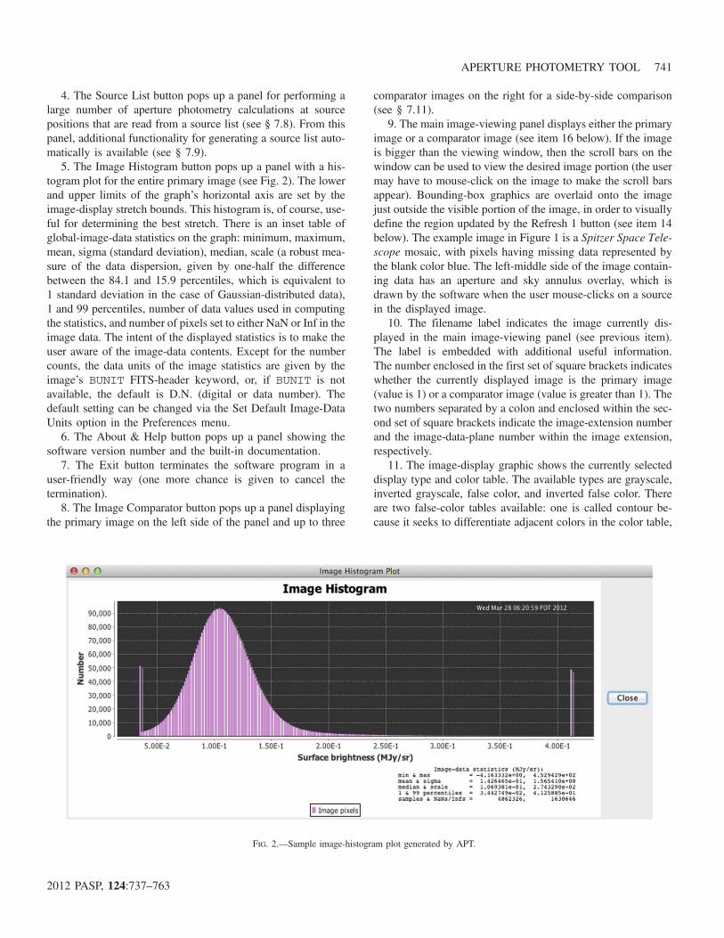
5. The Image Histogram button pops up a panel with a his-togram plot for the entire primary image (see Fig. 2). The lowerand upper limits of the graph’s horizontal axis are set by theimage-display stretch bounds. This histogram is, of course, use-ful for determining the best stretch. There is an inset table ofglobal-image-data statistics on the graph: minimum, maximum,mean, sigma (standard deviation), median, scale (a robust mea-sure of the data dispersion, given by one-half the differencebetween the 84.1 and 15.9 percentiles, which is equivalent to1 standard deviation in the case of Gaussian-distributed data),1 and 99 percentiles, number of data values used in computingthe statistics, and number of pixels set to either NaN or Inf in theimage data. The intent of the displayed statistics is to make theuser aware of the image-data contents. Except for the numbercounts, the data units of the image statistics are given by theimage’s BUNIT FITS-header keyword, or, if BUNIT is notavailable, the default is D.N. (digital or data number). Thedefault setting can be changed via the Set Default Image-DataUnits option in the Preferences menu.

6. The About & Help button pops up a panel showing thesoftware version number and the built-in documentation.

7. The Exit button terminates the software program in auser-friendly way (one more chance is given to cancel thetermination).

8. The Image Comparator button pops up a panel displayingthe primary image on the left side of the panel and up to three

comparator images on the right for a side-by-side comparison(see § 7.11).

9. The main image-viewing panel displays either the primaryimage or a comparator image (see item 16 below). If the imageis bigger than the viewing window, then the scroll bars on thewindow can be used to view the desired image portion (the usermay have to mouse-click on the image to make the scroll barsappear). Bounding-box graphics are overlaid onto the imagejust outside the visible portion of the image, in order to visuallydefine the region updated by the Refresh 1 button (see item 14below). The example image in Figure 1 is a Spitzer Space Tele-scope mosaic, with pixels having missing data represented bythe blank color blue. The left-middle side of the image contain-ing data has an aperture and sky annulus overlay, which isdrawn by the software when the user mouse-clicks on a sourcein the displayed image.

10. The filename label indicates the image currently dis-played in the main image-viewing panel (see previous item).The label is embedded with additional useful information.The number enclosed in the first set of square brackets indicateswhether the currently displayed image is the primary image(value is 1) or a comparator image (value is greater than 1). Thetwo numbers separated by a colon and enclosed within the sec-ond set of square brackets indicate the image-extension numberand the image-data-plane number within the image extension,respectively.

11. The image-display graphic shows the currently selecteddisplay type and color table. The available types are grayscale,inverted grayscale, false color, and inverted false color. Thereare two false-color tables available: one is called contour be-cause it seeks to differentiate adjacent colors in the color table,

FIG. 2.—Sample image-histogram plot generated by APT.

APERTURE PHOTOMETRY TOOL 741

2012 PASP, 124:737–763

and the other (eponymous) color table has a gradation of rain-bow colors. There are 24 levels of grayscale or 24 hues in thecolor tables. The display type and color table can be set via op-tions in the Preferences menu. See item 28 below for relatedinformation on the Color-Table Toggle button.

12. The image-magnifier panel displays a subimage of theimage currently shown in the main image-viewing panel. Thesubimage is centered at the mouse-cursor position in the mainimage-viewing panel. The subimage is changed in real time as themouse cursor is moved. The magnification options of the image-magnifier panel are 5×, 10× (the default setting), and 20×.

13. The Refresh 2 button repaints the image for both visibleand nonvisible portions of the image in the main image-viewingpanel. This is useful after image-display characteristics, such asthe stretch or color table, have been changed. After the shortamount of time required for this operation to complete, the mainimage-viewing panel’s scroll bars can be used to quickly scrollabout the entire image, which will be thereafter displayed withthe same image-viewing characteristics (until such time thatimage-viewing changes are made again).

14. The Refresh 1 button repaints the visible portion of theimage in the main image-viewing panel, plus the relatively smallnonvisible portion that lies within the bounding-box graphics(see item 9). This option is faster than the repainting of the entireimage done by the Refresh 2 button and is mainly useful for re-drawing the bounding-box graphics and eliminating any residualbounding-box graphics in the visible portion of the displayedimage. The latter can occur after the scroll-bar positions of themain image-viewing panel have been moved or after the mainGUI panel has been enlarged. For the most part, the visibleportion of the image is repainted automatically after changes toimage-viewing characteristics, such as the stretch or color table.

15. The Pick/Zap button pops up a panel with the pick/zaptool (see §7.7).

16. The Blink button is for image blinking the primary imageand up to three comparator images (see § 7.11).

17. The Thumbnail button pops up a panel that is capable ofdisplaying the entire primary image, rather than just the portionof it that may be currently displayed in the main image-viewingpanel. At the top of the thumbnail panel are a Show Grid buttonand a display of real-time mouse-cursor position in both imageand equatorial coordinates, as well as a display of the real-timepixel-data value at the cursor position. The Show Grid buttonwill overlay a grid labeled with equatorial coordinates and thensubsequently transform into a Hide Grid button. If a worldcoordinate system (WCS) is not available in the image’s FITSheader, then the grid overlay will be disabled. The thumbnailimage can be made to fit on the user’s computer screen usingthe Set Maximum Thumbnail Size option in the Preferencesmenu. If it is set to larger than the user’s screen, then the panelwill be automatically scaled to fit and scroll bars will appear.Figure 3 shows an example primary-image thumbnail with acoordinates-grid overlay.

18. The Recompute Photometry button repeats the aperturephotometry calculation after changes to its setup have beenmade, such as different aperture geometrical parameters. Suchchanges, which affect the results, cause the Recompute Photom-etry button text to change from the color black to the colorred as a reminder to the user that the calculation needs to beupdated. More details about how this button works and is usedare given in §§ 4, 6, 7.7, and 7.8.

19. The Plot Results button pops up a panel that allows thesetting up of scatter plots of one data column in the output aper-ture photometry table versus another. Histograms of data col-umns can also be plotted. Section 7.5 describes the availablefunctionality in more detail.

20. The List Results button pops up a spreadsheet-style list-ing of the output aperture photometry table. The data columns inthe table are fully described in § 7.4.

21. The Save Results button stores a record of the latest aper-ture photometry calculation as a single row in the outputaperture-photometry-table file. A calculation may be manuallyrepeated many times with different settings, but it is not saved inthe file until this button is utilized, and then only the last resultis saved.

22. The More Settings button pops up panel that enablesparametric changes to the aperture photometry calculation, in-cluding the specification of source and sky models. The optionsand controls on this panel are fundamental to utilizing APT toits fullest and are described in §§ 4, 5, and 6, as well asmentioned throughout the remainder of this article.

23. The main results of the latest aperture photometry calcu-lation are displayed near the lower-left corner of the main GUIpanel, under the heading PRIMARY-IMAGE PHOTOMETRYRESULTS. Section 7.4 defines the displayed quantities, whichare among the quantities written to the output aperture pho-tometry table when the user mouse-clicks on the Save Resultsbutton.

24. The Snap button nudges the aperture onto the computedcentroid of the source of interest (see § 6 for more details, in-cluding the color-coding).

25. The source’s centroid position, in floating-point pixels, isdisplayed just to the left of the Snap button (see § 6).

26. The aperture’s position, in integer pixels, is displayed inspinner-controllable text fields and can be changed here via ei-ther text-field editing or mouse-clicking on the tiny increment/decrement buttons located just to the right of the correspondingtext field.

27. The real-time pixel coordinates, the corresponding equa-torial coordinates, and the image-data value at the position of themouse cursor in the main image-viewing window are displayedunder the heading REAL-TIME RESULTS. The representationof the sky coordinates can be changed to either sexagesimal ordecimal degrees via theSet Celestial-Coordinates Units optionin the Preferences menu. The image-data units are given along-side the image-data value. The default image-data units are used

742 LAHER ET AL.

2012 PASP, 124:737–763

FIG. 3.—APT’s primary-image thumbnail.

APERTURE PHOTOMETRY TOOL 743

2012 PASP, 124:737–763

when the BUNIT keyword is absent from the image’s FITSheader and can be set via the Set Default Image-Data Units op-tion in the Preferences menu.

28. The six buttons on the left of the button group, ApertureSlice, Curve of Growth, Source Scatter, Radial Profile, SkyScatter, and Sky Histogram, pop up various graphs associatedwith the current calculation (see § 7.5). On the right, the HideAperture button temporarily hides the aperture overlay and sub-sequently transforms into the Show Aperture button and theColor-Table Toggle button that successively switches to theavailable presequenced color-table options (see item 11 above).

29. The Alter button next to the aperture-attributes label popsup a panel that allows changes to the elliptical aperture’s majorand minor radii and rotation angle (see Fig. 4), and the button’slabel indicates the values of these parameters. The text fields inthe group allow changes to values of the centroid, inner-sky, andouter-sky major radii, in integer pixels. The default apertureshape is circular, in fact, and the default settings for the centroid,aperture, inner-sky, and outer-sky radii are 5, 5, 8, and 15 pixels,respectively. These defaults can be changed via the Prefer-ences menu.

30. The Stretch-Type Toggle button cycles the image-displaystretch from linear to logarithmic to histogram equalization andthen back to linear.

31. The dynamic range slide control allows the dynamicrange of the logarithmic image-display stretch to vary from 0

(equivalent to a linear stretch) to 5 orders of magnitude (whichvisually differentiates the smallest image-data values that areabove the lower bound of the stretch). The default setting isone order of magnitude. The slide control is disabled for non-logarithmic types of stretches.

32. The stretch minimum and stretch maximum slide con-trols allow the lower and upper limits of the image-displaystretch, respectively, to be varied from their current settings.The new stretch is instantiated only after the Stretch to Boundsbutton is pressed (see next item).

33. The Stretch to Bounds button sets the limits of the image-display stretch to the two values in the lower-bound and upper-bound text fields (see next item).

34. The lower and upper limits of the current image-displaystretch can be manually changed by typing new values into thelower-bound and upper-bound text fields, respectively. The usermust either press Enter on the keyboard or mouse-click on theStretch to Bounds to apply changes made directly to these textfields.

4. BASIC USAGE INSTRUCTIONS

APT is intended to be simple to use. Basically, one displays aFITS image and then mouse-clicks on a source (i.e., an astro-nomical object) shown in the main image-viewing panel to over-lay an elliptical aperture onto it. The latter action causes thesoftware to automatically perform an aperture photometry cal-culation. The computed quantities include, among others,source centroid position, source intensity, source-intensity un-certainty, sky background level, and sky background dispersionwidth. The default sky algorithm is no sky background sub-traction from the source intensity, and the reason for this isto facilitate proper use of APT’s radial-profile interpolationcapability. More often than not, however, the user will requirethe sky background to be subtracted from the source intensity, inwhich case this sky model can be selected from the control panelthat pops up after mouse-clicking on the More Settings button(located in the lower-left corner of the main GUI panel; seealso item 22 in § 3). See Figure 5 for a depiction of the MoreSettings panel.

The general flow of the work progresses from the buttons andcontrols in the upper-left region of the main GUI panel to themiddle-left region and then lower-left region of the same. Hereare the basic instructions.

1. Take a moment to review the default settings by selectingList Preferences from the Preferences menu. More informa-tion on user preferences and how to change them is givenin § 7.2.

2. Choose a primary image to display by mouse-clicking onthe Get Image button in the upper-left corner of the GUI panel.The primary image, as defined here, is the first image displayedin the main image-viewing panel (after the primary image isloaded, a subsequent mouse-click on the Get Image button willFIG. 4.—APT’s panel for setting the elliptical-aperture attributes.

744 LAHER ET AL.

2012 PASP, 124:737–763

allow the user to load either a different primary image or com-parator images).

3. Adjust the image-display stretch for best viewing. As anaid, click on the Image Histogram button to see the stretch rangespanned by the image.

4. Select centroid and sky annulus major radii (integer valuesonly), and click on the Alter button beside the aperture-attributeslabel to select the elliptical aperture attributes, as appropriate forthe source of interest.

5. Place the mouse cursor over the source of interest in theimage displayed in the main image-viewing panel and click tooverlay an aperture.

6. Show and study the various graphs (instructions are givenin § 7.5).

7. Select the desired new radii, as appropriate, and/or changeother settings as needed.

8. Redraw or overlay a new aperture by either clickingon the Recompute Photometry button or clicking on theSnap button for nudging the aperture onto the source cen-troid location or placing the mouse cursor on the image andclicking.

9. If necessary, increment or decrement the spinner controlsfor fine-tuning the aperture’s position.

10. Click on the Recompute Photometry button to redraw/overlay a new aperture.

11. Show and study the various graphs again.12. Optionally click on the Save Results button, located in

the lower-left corner of the main GUI panel, in order to save/append the results to APT’s output photometry-table file (e.g.,APT.tbl). The adjacent List Results and Plot Results buttons canbe used to list and plot the saved results.

13. Repeat the above steps for each source of interest.

FIG. 5.—APT’s More Settings panel.

APERTURE PHOTOMETRY TOOL 745

2012 PASP, 124:737–763

5. SKY BACKGROUND ESTIMATION

Strictly speaking, the background should be the best estimateof the true underlying background emission, excluding contam-ination from the source flux being measured, and not biased byany other neighboring sources or outliers. As a practical matter,we estimate the background in the aperture from an ellipticalsky annulus surrounding it, and this method does not accountfor gradients in the sky background caused by sources in theannulus. A bright source in the sky annulus contributes tothe background in the aperture, and its effect is not necessarilysomething that is to be completely ignored or filtered out, whichis why APT has a variety of sky models from which to choose.

APT has fairly straightforward methods for estimating thesky background in the region local to the source of interest,and there are a few options available for controlling how itis done. Only image pixels in an elliptical sky annulus centeredon a user-selected center position are considered for the back-ground calculation. The pixels with NaN or Inf are rejectedoutright. The center position, for purposes of background esti-mation, is specified in integer pixels only. There are three dif-ferent ways of specifying the center position in APT:

1. Mouse-clicking on the image displayed in the main image-viewing panel.

2. Changing the values in the spinner-controllable text fieldsfor the aperture position, which are located near the lower-leftcorner of the main GUI panel.

3. Clicking on the Snap button in the lower-left corner of themain GUI panel (more on this in § 6).

The inner and outer major radii of the sky annulus, in integerpixels only, can be specified on the main GUI panel. Thesemajor radii are used to scale the ellipse specified for the aper-ture. The inner radius of the sky annulus must be greater than orequal to the radius of the elliptical aperture along any directionfrom the center of the ellipse. No limitation is placed on theouter radius of the sky annulus, except that it must be greaterthan the inner radius. The default values that specify the size andshape of the aperture and sky annulus, which are loaded whenAPT is launched, can be specified via the Set Photometry SizeParameters option under the Preferences menu.

On the APT control panel that pops up after clicking on theMore Settings button, the user can select from one of four avail-able sky models:

Model A.—No sky background subtraction.Model B.—Sky median subtraction.Model C.—Custom sky subtraction.Model D.—Sky average subtraction.Sky median subtraction is less sensitive than sky average

subtraction to other bright sources that may fall within the skyannulus, which might otherwise cause the background to beoverestimated. If model C is specified, then the custom valueto be used must be specified in the text field labeled Customsky value on the More Settings panel.

The More Settings panel has text fields where the user canoptionally specify lower and upper thresholds for the rejectionof outlier pixels in the sky annulus from the background calcu-lation. The default values for the lower and upper thresholds arethe largest possible negative and positive double-precision num-bers, respectively, so that, by default, no pixels are rejected. Thevalues for the outlier-rejection thresholds must be given in thedata units of the image’s FITS file. It is best to study the variousaperture photometry graphs provided by APT, in order to figureout the best thresholds, and then set these thresholds beforeoptionally converting the image-data units into the desiredsource-intensity units (see § 7.5 for how to do the latter).

In addition to the aforementioned outlier rejection, there isyet another outlier-rejection method that is applied. The medianand standard deviation are computed, and all data values that liegreater than 3 standard deviations from the median are rejected.Currently, this number of standard deviations is hard-coded andcannot be changed by the user.

The pixel zap functionality of the pick/zap tool can also beused to temporarily eliminate pixels from the background cal-culation. More details about the pick/zap tool are given in § 7.7.

The median and average of the remaining image data in thesky annulus after the outlier rejection have been applied arecomputed as possible background estimators. The median oraverage times the number of pixels in the aperture form a pro-duct that is the sky contribution optionally subtracted from theintegrated image data of the source to get the background-subtracted source intensity. These quantities are labeled Sky_median/pix and Sky_average/pix, respectively, in the outputaperture photometry table (see § 7.4). The standard deviationis computed for the Sky_sigma column in the aperture photom-etry table. Likewise, the root-mean-squared (rms) value is com-puted for the Sky_RMS/pix column. The Sky_scale column, arobust estimator of the data dispersion, is computed as one-halfof the difference between the 84 and 16 data percentiles.

6. APERTURE PHOTOMETRY IMPLEMENTATION

The aperture photometry calculation primarily yields thesource intensity and its uncertainty. The former involves sum-ming pixel values within the aperture to get the total intensity,then subtracting the product of the aperture area, in pixels2, andthe per-pixel sky background, in order to get the source inten-sity. The latter also requires the aperture and sky annulus geom-etry, as well as extra information, including the detector gain,the conversion factor from image-data units to D.N. (if imageis not already in units of D.N.), the background-estimationmethod, and the sky background standard deviation. APTworksunder the assumption that the background is constant across theaperture.

APT performs its calculations with an elliptical aperture,which the user specifies with major and minor radii and a rota-tion angle. These quantities are recorded in the MajR_aper,MinR_aper, and Rot_aper columns, respectively, in the output

746 LAHER ET AL.

2012 PASP, 124:737–763

aperture photometry table (see § 7.4). Of course, APT alsoallows circular apertures, as a circle is a special case of an ellipsewith its major radius equal to its minor radius.

The basic inputs for the calculation are the elliptical-aperturegeometrical parameters, the source centroid major radius, andposition coordinates of the aperture center (the instructionsfor selecting these quantities are given in § 5). The calculationof the source’s centroid position, which shares the same centerposition as the aperture, can involve a different number of pixelsthan used in the calculation. The source centroid ellipse is itsmajor radius scaled to the ellipse specified for the aperture.The aperture geometrical parameters and centroid major radiuscan be specified on the main GUI panel.

The More Settings panel has text fields where the user canoptionally specify lower and upper thresholds for rejection ofspurious aperture pixels in the calculation. The default valuesfor the lower and upper thresholds are the largest possiblenegative and positive double-precision numbers, respectively,so that, by default, no pixels are rejected. Again, values foroutlier-rejection thresholds must be given in image-data units.

The pixel zap functionality of the pick/zap tool can also beused to temporarily eliminate pixels from the calculation. Moredetails about the pick/zap tool are given in § 7.7.

The method that computes the source centroid position isiterative and runs for 100 iterations. The first iteration is boot-strapped from the user-selected aperture position. The kþ 1thiteration computes the following x and y image coordinates ofthe source centroid:

xkþ1centroid ¼ xk

centroid þ

Pi;j∈SðkÞ

ðxi � xkcentroidÞðdij � dkminÞPi;j∈SðkÞ

ðdij � dkminÞ; (1)

and

ykþ1centroid ¼ ykcentroid þ

Pi;j∈SðkÞ

ðyj � ykcentroidÞðdij � dkminÞPi;j∈SðkÞ

ðdij � dkminÞ; (2)

where the sums are over pixels in the centroid ellipse SðkÞ thatmeet criteria given below; image data value dij is located at pix-el (xi, yj); and dkmin is the smallest data value in the centroidellipse. The data values included in the summing must be great-er than dkmin, not NaN or Inf, and less than or equal to the upperoutlier-rejection threshold for the calculation. The centroidellipse is allowed to move with each iteration, so it is necessaryto recompute dkmin each time. The centroid calculation is donewith subpixel resolution, but the step size is currently limited tono less than 0.05 pixels for computational speed. The methodgenerally converges for isolated sources, but not always, and theuser is cautioned to check that the resulting source centroid is areasonable one. The source centroid calculation does not always

give the best aperture position for the source of interest, espe-cially if there are other sources nearby that fall within thecentroid ellipse. One can use visual feedback from the aper-ture-slice and source-scatter graphs for improved manual aper-ture positioning. See § 7.5 for more information about theavailable APT graphs.

The More Settings panel has radio buttons for the user toselect one of three available source models:

Model 0.—No aperture interpolation.Model 1.—Aperture interpolation only for NaN and Inf pix-

els (including zapped pixels).Model 2.—Interpolation for all aperture pixels.Model 0 will underestimate the source intensity if there are a

significant number of blank pixels in the aperture. Model 1 wasdesigned to remedy this, but it requires that the user set up aradial-profile model for the interpolation, and APT has a toolthat makes it easy (as discussed in § 7.6). Model 2 uses theradial-profile model to compute data values for all pixels in theaperture and generally gives a result that is within a few percentor better of model 0 if the radial-profile model was set up on thesame source. Model 2 is most useful in cases where the sourceof interest has missing aperture pixels and the radial-profilemodel was set up on a different source that has no missing pix-els, which is facilitated by the built-in automatic scaling andoffsetting of the radial profile.

The aperture photometry calculation is done with subpixelresolution. The default subpixel size is 0.01 pixels. The smallvalue can cause the computations to take several seconds forvery large aperture ellipses. The subpixel size can be changedvia the Set Calculation Step Size option in the Preferences menu.

By default, the calculation is performed with the aperturecentered on the calculated source centroid. The CentroidðX; Y Þ ¼ label on the lower-left side of the main GUI panelis displayed in the color green to indicate that centroiding isenabled and in the color black to indicate that it is disabled.Unchecking the Use centroid in photometry calculation? checkbox on the More Settings panel will do the disabling and causethe calculation to revert to centering the aperture on the integerpixel coordinates of the selected aperture position. Note thatalthough centroiding moves the center position of the aperturewith subpixel resolution, the center position of the sky annulusis incremented only with integer-pixel resolution.

The Snap button in the lower-left main GUI panel is availableto nudge the aperture onto the computed source centroid loca-tion. After moving the aperture, it automatically recomputes thephotometric results (just like the Recompute Photometry but-ton). If centroiding is turned on and the aperture is already fairlyclose to the centroid, the recomputation may give the same non–background-subtracted source intensity as before (with slightchanges possible to the source-intensity uncertainty, sky back-ground, and sky background dispersion), and the main differ-ence will be that the aperture will appear to be bettercentered on the centroid position (and the data points plotted

APERTURE PHOTOMETRY TOOL 747

2012 PASP, 124:737–763

in most of the APT graphs will be shifted accordingly). If cen-troiding is turned off, the user will obtain a new result at the newaperture position, which, after snapping the aperture, will bethe centroid position represented by integer image coordinates.The Snap button text will turn the color yellow to remind theuser to mouse-click on this button to fully center the aperture onthe centroid location. This color reminder can and should beignored if the user wants photometric results for an aperture thatis dislocated from the centroid position, in which case centroid-ing should be turned off.

The source-intensity-uncertainty calculation requires thedetector gain (electrons per D.N.), the conversion factor fromimage-data units to D.N., and the depth of coverage. The defaultvalue for these quantities is 1.0. When a primary image isloaded, the software attempts to read the GAIN FITS keywordand, if found, automatically overrides the default gain value. Forimage data that are already in units of D.N., the value of 1.0 isappropriate for the image-data-units-to-D.N. conversion factor.A depth of coverage of 1.0 is correct for a single observation.These quantities can be subsequently overridden on the MoreSettings panel, after an image has been loaded. The default gainvalue, used in the absence of the GAIN FITS keyword, can bechanged via the Set Default Image-Data Gain option in the Pref-erences menu.

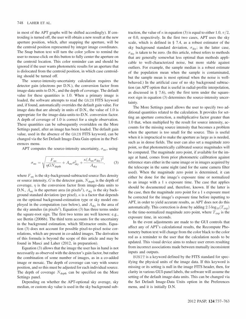
APT computes the source-intensity uncertainty, σsrc, using

σsrc ¼ffiffiffiffiffiffiffiffiffiffiffiffiffiffiffiffiffiffiffiffiffiffiffiffiffiffiffiffiffiffiffiffiffiffiffiffiffiffiffiffiffiffiffiffiffiffiffiffiffiffiffiffiffiffiffiffiffiffiffiffiffiffiffiffiffiffiffiffiffi

F src

ηGNdepthþAsrcσ2

sky þκðAsrcσskyÞ2

Asky

s; (3)

where F src is the sky-background-subtracted source flux densityor source intensity, G is the detector gain, Ndepth is the depth ofcoverage, η is the conversion factor from image-data units toD.N., Asrc is the aperture area (in pixels2), σsky is the sky back-ground standard deviation (per pixel), κ is a factor that dependson the optional background-estimation type or sky model em-ployed in the computation (see below), and Asky is the area ofthe sky annulus (in pixels2). Equation (3) has three terms underthe square-root sign. The first two terms are well known: e.g.,see Bertin (2006b). The third term accounts for the uncertaintyin the background estimation, which SExtractor omits. Equa-tion (3) does not account for possible pixel-to-pixel noise cor-relations, which are present in co-added images. The derivationof this formula is beyond the scope of this article and may befound in Masci and Laher (2012, in preparation).

Equation (3) allows that the image the user has in hand is notnecessarily as observed with the detector’s gain factor, but ratherthe combination of some number of images, as in a co-addedimage or mosaic. The depth of coverage can vary with sourceposition, and so this must be adjusted for each individual source.The depth of coverage Ndepth can be specified on the MoreSettings panel.

Depending on whether the APT-optional sky average, skymedian, or custom sky value is used in the sky background sub-

traction, the value of κ in equation (3) is equal to either 1.0, π=2,or 0.0, respectively. In the first two cases, APT uses the skyscale, which is defined in § 7.4, as a robust estimator of thesky background standard deviation, σsky; in the latter case,σsky is taken to be zero. (In this article, robust refers to methodsthat are generally somewhat less optimal than methods appli-cable to well-characterized noise, but more stable againstoutliers. For example, the sample median is a robust estimateof the population mean when the sample is contaminated,but the sample mean is most optimal when the noise is well-behaved.) In the artificial case of no sky background subtrac-tion (an APT option that is useful in radial-profile interpolation,as discussed in § 7.6), only the first term under the square-root sign in equation (3) determines the source-intensity uncer-tainty.

The More Settings panel allows the user to specify two ad-ditional quantities related to the calculation. It provides for set-ting an aperture correction, a multiplicative factor greater than1.0 that, when multiplied by the result for source intensity, ac-counts for the missing source intensity that becomes a problemwhen the aperture is too small for the source. This is usefulwhen it is impractical to make the aperture as large as is needed,such as in dense fields. The user can also set a magnitude zeropoint, so that photometrically calibrated source magnitudes willbe computed. The magnitude zero point, if available for the im-age at hand, comes from prior photometric calibration againstreference stars either in the same image or in images acquired bythe telescope in the same night (and for the same camera filterused). When the magnitude zero point is determined, it caneither be done for the image’s exposure time or normalizedto an image with a 1 s exposure time. The case that appliesshould be documented and, therefore, known. If the latter isthe case, then the magnitude zero point for a 1 s exposure mustbe corrected for the image’s exposure time before inputting toAPT, in order to yield accurate results, as APT does not do thisautomatically. This correction is done by adding 2:5 log10ðT expÞto the time-normalized magnitude zero point, where T exp is theexposure time, in seconds.

In the event adjustments are made to the GUI controls thataffect any of APT’s calculational results, the Recompute Pho-tometry button text will change from the color black to the colorred as a reminder to the user that the calculation needs to beupdated. This visual device aims to reduce user errors resultingfrom incorrect associations made between mutually inconsistentinputs and outputs.

BUNIT is a keyword defined by the FITS standard for spec-ifying the physical units of the image data. If this keyword ismissing or its setting is null in the image FITS header, then, forclarity in various GUI-panel labels, the software will assume thesetting of the default image-data units. This can be changed viathe Set Default Image-Data Units option in the Preferencesmenu, and it is initially D.N.

748 LAHER ET AL.

2012 PASP, 124:737–763

7. SUPPLEMENTARY SOFTWARE FUNCTIONALITY

7.1. Image-Data Display

In the main image-viewing panel, which is located in theupper-right corner of the main GUI panel, the stretch and color-table controls work automatically only for the visible portion ofthe displayed image, plus some margin around the visibleimage’s edges. This design feature allows the software to runfaster and be more responsive. The positions of the panel’sscroll bars determine which portion of the image is visibleand actively updated when the image-viewing settings arechanged. Moving the scroll bars for large images will revealthe once-active portion of the image inside a visually obviousbounding box. The image outside of the bounding box will bedisplayed with a different stretch and/or color table, which wasset earlier in the APT session. To remove the unsightly remnantsof the bounding box and refresh the displayed image, two re-fresh options are available. The Refresh 1 button quickly re-freshes just the visible portion of the image to save time.The Refresh 2 button refreshes the entire image by launchingmultiple processor threads for refreshing the unseen portionof the image, so that immediate GUI control is returned tothe user, and additional computer CPU cores, if available onthe user’s machine, are utilized to finish the job faster. For verylarge images, however, the threads take some time to completeand may still be running even though the user is allowed to con-tinue normal work with the GUI. To avoid queueing up toomany threads, the user is advised to not mouse-click on the Re-fresh 2 button more than once in a reasonable time interval: atleast a few seconds. When needed, the Refresh 2 button text willchange from the color black to the color yellow to remind theuser to click on this button before scrolling about the image. It isnot mandatory for the user to click on the Refresh 2 button whenits text turns yellow; the user can defer doing this until after thescroll bars are subsequently moved.

For purposes of image display only, all image-data valuesoutside the interval specified by the stretch extrema are setto the corresponding extreme value. Image-data values thatare set to NaN or Inf are displayed with the blank color setby the user (the color blue is the default). Inf values are handledthe same as NaN values, and almost no distinction is made be-tween these two bad-data types. The blank color can be changedusing the blank color-picker accessible via the Set Image-Display Attributes option in the Preferences menu.

The user can specify the maximum image size that the soft-ware will load into memory. This is done using the SetMaximum Image Size option in the Preferences menu. The de-fault maximum image size is 5000 pixels on an image side, andthis preference can be reset to as many as 100,000 pixels. Forimages larger than the preferred value, the user will be promptedto specify the desired portion of the image after its filename hasbeen selected.

7.2. User Preferences

Various options in the Preferences menu allow users tochange the default settings and then save them to disk for a laterAPT session. When APT is launched, it automatically loads thepreferences from a special file called APT.pref that is located inthe invisible subdirectory called .AperturePhotometryTool inthe user’s home directory.15 Users also have the option of latermanually loading in another preferences file from a differentdisk location and filename. If the special preferences file doesnot exist, then factory-default preferences are loaded into theuser’s session, but are not automatically saved—the user mustexplicitly save them via the Save Preferences option in the Pref-erences menu, if that is what the user wants to do. Within agiven APT session, whenever a new primary image is readin, the preferences are restored from the special preferences file.Selecting the Reset Default Preferences option in the Prefer-ences menu will restore the factory-default settings to the user’ssession, but will not save them (again, the user must manuallyselect the option to do this). If the Save Preferences option isselected, then the current settings of the user’s session willbe written to a user-selected location and filename, and if thatfile already exists, then all prior custom settings in that file willbe overwritten.

At any time during a user’s session, most of the currentsettings, as set by the various GUI controls within and withoutthe Preferences menu, are the instantaneous user’s preferencesfor the session (albeit not necessarily saved to disk). This can beverified by mouse-clicking on the List Preferences function un-der the Preferences Menu. One exception is the setting of theaperture geometrical parameters and the centroid and sky annu-lus inner and outer major radii, whose preferred values shouldbe set via the Set Aperture Size, Shape, and Angle and SetPhotometry Size Parameters options in the Preferences menu(these values may be changed to other values directly on themain GUI panel, as needed for experimentation, without affect-ing the preferences). Therefore, the Save Preferences optionwill, for the most part, capture the current state of the user’ssession.

7.3. Output Files

During the operation of the software, several output files arecreated at various stages (see Table 1). With the exceptionsnoted below, all output files are created in the scratch directorywith fixed filenames. The output aperture-photometry-table disklocation and filename, the location of the scratch directory, andthe user-preferences location and filename can be changed viaoptions available in the Preferences menu. The filenamesourceListByAPT.dat is, by default, generated in the last

15Note that the environment variable APT_HOME must be set to the locationwhere APT is installed, and this location is not to be confused with the user’shome directory.

APERTURE PHOTOMETRY TOOL 749

2012 PASP, 124:737–763

directory from which a source-list file was read by the source-list tool (see § 7.8), or, if this is not available, the scratch direc-tory; there is also the user option on the source-list-creationpanel of selecting the location and filename of choice for thenewly generated source list (see § 7.9).

7.4. Aperture Photometry Table

APT generates a table of accumulated results during thecourse of its normal operation. This is not automatic, however;the user must deliberately mouse-click on the Save Results but-ton after each aperture photometry calculation, in order to writea row of results to the table. Users can save the table to the disklocation and filename of their choice. The default location is theinvisible subdirectory .AperturePhotometryTool in the user’shome directory and the default filename is APT.tbl. Table 2defines the columns of the table, along with applicable dataunits, in the order the columns appear in the table. The tablecan be listed by mouse-clicking on the List Results button lo-cated in the lower-left corner of the main GUI panel. The table’sdata are stored in a plain-text file, which can be easily parsedwith a user-supplied script.

7.5. Graphs

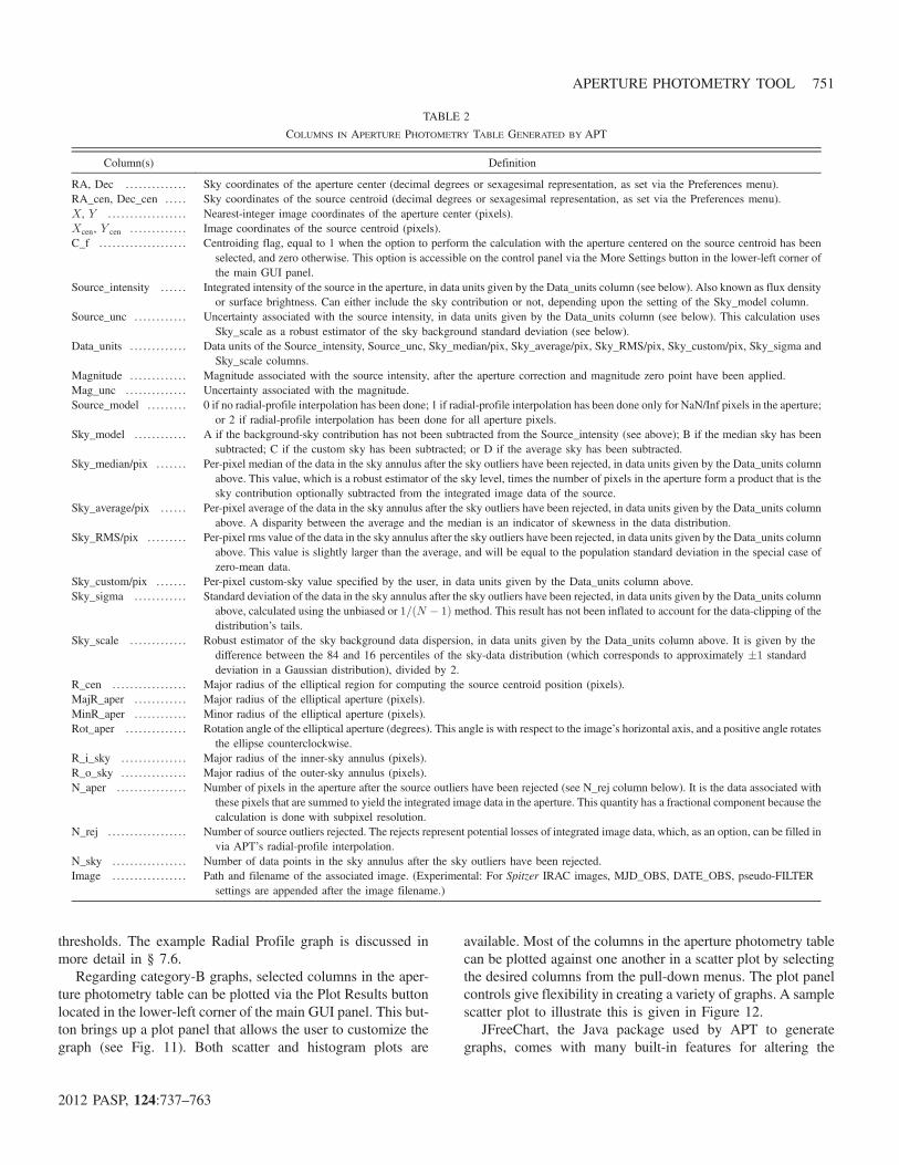
APT produces three different general categories of graphs.One is simply the aforementioned image histogram, which doesnot fit into the two remaining categories (see item 5 in § 3, andFig. 2). Another is a set of different graphs that pertain to thecurrent aperture photometry calculation (category A). The otheris the capability of making scatter plots and histograms of user-selected columns in the output aperture photometry table (cate-gory B). Category-A graphs are most useful for analyzing andrefining the current calculation, and category-B graphs are forvisualizing a set of calculations, such as might cover a largenumber of sources extracted from a given image.

There are six different category-A graphs, and these are eas-ily displayed by mouse-clicking on the associated main-GUI-

panel buttons located in the middle of the main GUI panel(see item 28 in § 3). The choices are Aperture Slice, Curveof Growth, Source Scatter, Sky Scatter, Sky Histogram, andRadial Profile. All of these graphs require that an aperture beoverlaid onto the primary image as described above. The graphsmay be selected in any order, although the order listed above is agood one for adjusting APT settings systematically for a givensource.

There is a text field near the middle of the More Settingspanel labeled Default image-data title for the user to specifythe graph’s image-data title (e.g., Surface brightness). At thebottom of the More Settings panel, there are options that controlthe data plotted in the category-A graphs. There is a check boxlabeled Perform image-data conversion that enables the conver-sion of the image data from the image-data units of the FITS fileto any desired source-intensity units. In addition, there are as-sociated text fields for specifying the conversion factor, a stringrepresentation of the physical units (e.g., MJy sr�1), and a stringrepresentation of the graph image-data title for the convertedimage data (e.g., flux density). The latter, if the check box isenabled, will override the default image-data title.

Figure 6 shows an Aperture Slice plot generated by APT. Theblue and pink curves correspond to slices through the aperturecenter along horizontal and vertical image axes, respectively.The slices extend across both aperture and sky annulus. Alongwith the plotted curves are colored lines that visually convey thesize and shape of the aperture and sky annulus. All verticalcolored lines in the plot map directly to the colors used inthe overlay symbol representing the aperture and sky annuluson the image.

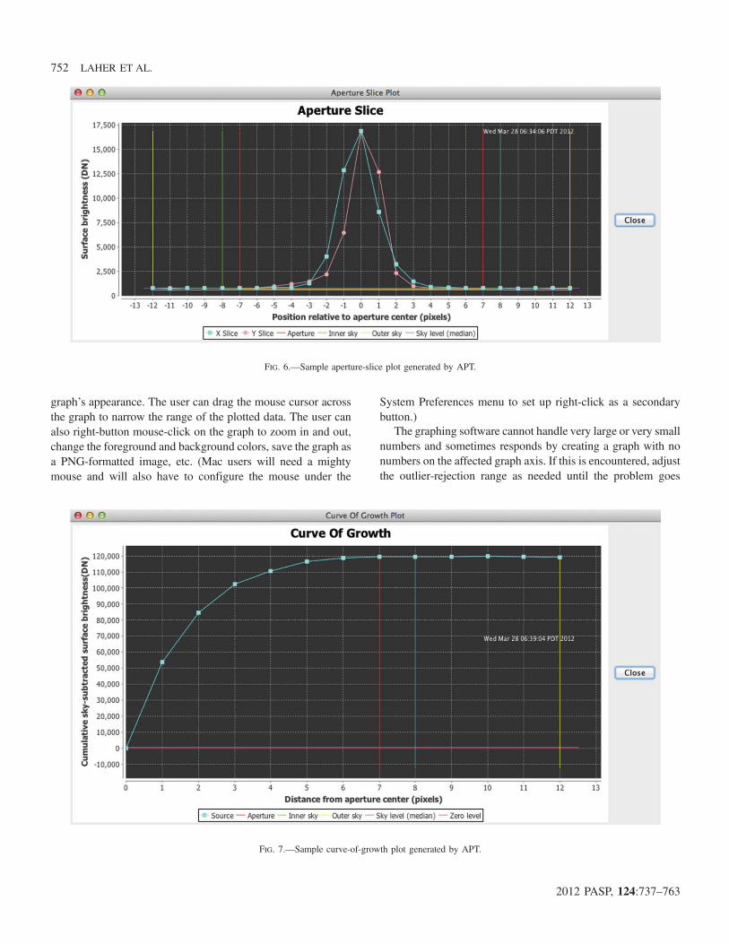
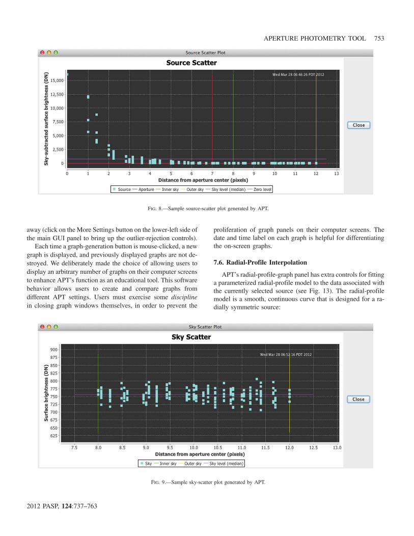
Figures 7—10 give random examples of the other category-A graphs available. The Curve of Growth graph is useful fordetermining the best aperture and sky annulus major and minorradii (assuming the rotation angle of the elliptical aperture isset correctly). The Source Scatter, Sky Scatter, and Sky Histo-gram graphs are useful in setting efficacious outlier-rejection

TABLE 1

OUTPUT FILES CREATED BY APT

Filename Definition

APT.pref . . . . . . . . . . . . . . . . . . . . . . . . . . . Default filename of customizable user preferences (see § 7.2).APT.tbl . . . . . . . . . . . . . . . . . . . . . . . . . . . . Default filename of output aperture photometry table (see § 7.4).fitsHdr.txt . . . . . . . . . . . . . . . . . . . . . . . . . . Listing of the FITS header.apertureSliceX.dat . . . . . . . . . . . . . . . . . Image data corresponding to a horizontal slice across the aperture.apertureSliceY.dat . . . . . . . . . . . . . . . . . Image data corresponding to a vertical slice across the aperture.skyScatter.dat . . . . . . . . . . . . . . . . . . . . . . Data shown in the sky-scatter graph.sourceScatter.dat . . . . . . . . . . . . . . . . . . Data shown in the source-scatter graph.curveOfGrowth.dat . . . . . . . . . . . . . . . . Data shown in the curve-of-growth graph.radialProfile.dat . . . . . . . . . . . . . . . . . . . Data shown in the radial-profile graph.radialProfileDataFitCurve.dat . . . . . Data-fit curve shown in the radial-profile graph.radialProfileDataFitModel.dat . . . . . Data-fit model for aperture interpolation (see § 7.6).scatter.dat . . . . . . . . . . . . . . . . . . . . . . . . . . Scatter-plot data from user-selected columns in the aperture photometry table.sourceListByAPT.dat . . . . . . . . . . . . . Source-list file generated by APT’s extraction of image sources (see § 7.9).

750 LAHER ET AL.

2012 PASP, 124:737–763

thresholds. The example Radial Profile graph is discussed inmore detail in § 7.6.

Regarding category-B graphs, selected columns in the aper-ture photometry table can be plotted via the Plot Results buttonlocated in the lower-left corner of the main GUI panel. This but-ton brings up a plot panel that allows the user to customize thegraph (see Fig. 11). Both scatter and histogram plots are

available. Most of the columns in the aperture photometry tablecan be plotted against one another in a scatter plot by selectingthe desired columns from the pull-down menus. The plot panelcontrols give flexibility in creating a variety of graphs. A samplescatter plot to illustrate this is given in Figure 12.

JFreeChart, the Java package used by APT to generategraphs, comes with many built-in features for altering the

TABLE 2

COLUMNS IN APERTURE PHOTOMETRY TABLE GENERATED BY APT

Column(s) Definition

RA, Dec . . . . . . . . . . . . . . Sky coordinates of the aperture center (decimal degrees or sexagesimal representation, as set via the Preferences menu).RA_cen, Dec_cen . . . . . Sky coordinates of the source centroid (decimal degrees or sexagesimal representation, as set via the Preferences menu).X, Y . . . . . . . . . . . . . . . . . . Nearest-integer image coordinates of the aperture center (pixels).Xcen, Y cen . . . . . . . . . . . . . Image coordinates of the source centroid (pixels).C_f . . . . . . . . . . . . . . . . . . . . Centroiding flag, equal to 1 when the option to perform the calculation with the aperture centered on the source centroid has been

selected, and zero otherwise. This option is accessible on the control panel via the More Settings button in the lower-left corner ofthe main GUI panel.

Source_intensity . . . . . . Integrated intensity of the source in the aperture, in data units given by the Data_units column (see below). Also known as flux densityor surface brightness. Can either include the sky contribution or not, depending upon the setting of the Sky_model column.

Source_unc . . . . . . . . . . . . Uncertainty associated with the source intensity, in data units given by the Data_units column (see below). This calculation usesSky_scale as a robust estimator of the sky background standard deviation (see below).

Data_units . . . . . . . . . . . . . Data units of the Source_intensity, Source_unc, Sky_median/pix, Sky_average/pix, Sky_RMS/pix, Sky_custom/pix, Sky_sigma andSky_scale columns.

Magnitude . . . . . . . . . . . . . Magnitude associated with the source intensity, after the aperture correction and magnitude zero point have been applied.Mag_unc . . . . . . . . . . . . . . Uncertainty associated with the magnitude.Source_model . . . . . . . . . 0 if no radial-profile interpolation has been done; 1 if radial-profile interpolation has been done only for NaN/Inf pixels in the aperture;

or 2 if radial-profile interpolation has been done for all aperture pixels.Sky_model . . . . . . . . . . . . A if the background-sky contribution has not been subtracted from the Source_intensity (see above); B if the median sky has been

subtracted; C if the custom sky has been subtracted; or D if the average sky has been subtracted.Sky_median/pix . . . . . . . Per-pixel median of the data in the sky annulus after the sky outliers have been rejected, in data units given by the Data_units column

above. This value, which is a robust estimator of the sky level, times the number of pixels in the aperture form a product that is thesky contribution optionally subtracted from the integrated image data of the source.

Sky_average/pix . . . . . . Per-pixel average of the data in the sky annulus after the sky outliers have been rejected, in data units given by the Data_units columnabove. A disparity between the average and the median is an indicator of skewness in the data distribution.

Sky_RMS/pix . . . . . . . . . Per-pixel rms value of the data in the sky annulus after the sky outliers have been rejected, in data units given by the Data_units columnabove. This value is slightly larger than the average, and will be equal to the population standard deviation in the special case ofzero-mean data.

Sky_custom/pix . . . . . . . Per-pixel custom-sky value specified by the user, in data units given by the Data_units column above.Sky_sigma . . . . . . . . . . . . Standard deviation of the data in the sky annulus after the sky outliers have been rejected, in data units given by the Data_units column

above, calculated using the unbiased or 1=ðN � 1Þ method. This result has not been inflated to account for the data-clipping of thedistribution’s tails.

Sky_scale . . . . . . . . . . . . . Robust estimator of the sky background data dispersion, in data units given by the Data_units column above. It is given by thedifference between the 84 and 16 percentiles of the sky-data distribution (which corresponds to approximately �1 standarddeviation in a Gaussian distribution), divided by 2.

R_cen . . . . . . . . . . . . . . . . . Major radius of the elliptical region for computing the source centroid position (pixels).MajR_aper . . . . . . . . . . . . Major radius of the elliptical aperture (pixels).MinR_aper . . . . . . . . . . . . Minor radius of the elliptical aperture (pixels).Rot_aper . . . . . . . . . . . . . . Rotation angle of the elliptical aperture (degrees). This angle is with respect to the image’s horizontal axis, and a positive angle rotates

the ellipse counterclockwise.R_i_sky . . . . . . . . . . . . . . . Major radius of the inner-sky annulus (pixels).R_o_sky . . . . . . . . . . . . . . . Major radius of the outer-sky annulus (pixels).N_aper . . . . . . . . . . . . . . . . Number of pixels in the aperture after the source outliers have been rejected (see N_rej column below). It is the data associated with

these pixels that are summed to yield the integrated image data in the aperture. This quantity has a fractional component because thecalculation is done with subpixel resolution.

N_rej . . . . . . . . . . . . . . . . . . Number of source outliers rejected. The rejects represent potential losses of integrated image data, which, as an option, can be filled invia APT’s radial-profile interpolation.

N_sky . . . . . . . . . . . . . . . . . Number of data points in the sky annulus after the sky outliers have been rejected.Image . . . . . . . . . . . . . . . . . Path and filename of the associated image. (Experimental: For Spitzer IRAC images, MJD_OBS, DATE_OBS, pseudo-FILTER

settings are appended after the image filename.)

APERTURE PHOTOMETRY TOOL 751

2012 PASP, 124:737–763

graph’s appearance. The user can drag the mouse cursor acrossthe graph to narrow the range of the plotted data. The user canalso right-button mouse-click on the graph to zoom in and out,change the foreground and background colors, save the graph asa PNG-formatted image, etc. (Mac users will need a mightymouse and will also have to configure the mouse under the

System Preferences menu to set up right-click as a secondarybutton.)

The graphing software cannot handle very large or very smallnumbers and sometimes responds by creating a graph with nonumbers on the affected graph axis. If this is encountered, adjustthe outlier-rejection range as needed until the problem goes

FIG. 6.—Sample aperture-slice plot generated by APT.

FIG. 7.—Sample curve-of-growth plot generated by APT.

752 LAHER ET AL.

2012 PASP, 124:737–763

away (click on the More Settings button on the lower-left side ofthe main GUI panel to bring up the outlier-rejection controls).

Each time a graph-generation button is mouse-clicked, a newgraph is displayed, and previously displayed graphs are not de-stroyed. We deliberately made the choice of allowing users todisplay an arbitrary number of graphs on their computer screensto enhance APT’s function as an educational tool. This softwarebehavior allows users to create and compare graphs fromdifferent APT settings. Users must exercise some disciplinein closing graph windows themselves, in order to prevent the

proliferation of graph panels on their computer screens. Thedate and time label on each graph is helpful for differentiatingthe on-screen graphs.

7.6. Radial-Profile Interpolation

APT’s radial-profile-graph panel has extra controls for fittinga parameterized radial-profile model to the data associated withthe currently selected source (see Fig. 13). The radial-profilemodel is a smooth, continuous curve that is designed for a ra-dially symmetric source:

FIG. 8.—Sample source-scatter plot generated by APT.

FIG. 9.—Sample sky-scatter plot generated by APT.

APERTURE PHOTOMETRY TOOL 753

2012 PASP, 124:737–763

SðrÞ ¼ Aþ Brþ Cr2 þDr3 þ Er4 þ F exp

��r2

2σ2

�; (4)

where SðrÞ is the pixel intensity or surface brightness as afunction of radial distance from the aperture center r, in pixels,which is constrained by r ≥ 0; the data-fit coefficientsA throughF are determined via linear regression; and σ is a fixed parameterthat can be manually adjusted to optimize the data fit. The right-most term containing the exponential function is a scaled Gaus-sian distribution, and σ, therefore, is the familiar measure of thedistribution’s half-width. This model was deliberately chosen tobe relatively simple and yet have enough degrees of freedom towork well on images with a point-spread function (PSF) that isby-and-large radially symmetric. Optimizing the data fit involvesmanually choosing the value of σ that minimizes the least-squared-error goodness-of-fit measure χ2.

In order to build a model for the image of interest, the usermust adhere to the following instructions precisely:

1. On the More Settings panel (accessed via the More Set-tings button on the lower-left part of the main GUI panel), selectthe Model 0 source algorithm and the Model A sky algorithm.Also, the check box labeled Perform new image-data conversionon the More Settings panel should be unchecked. A picture ofthe More Settings panel is shown in Figure 5. Warnings will begiven when the model is saved with these conditions not met.

2. Select a source fromwhich to create the radial-profile mod-el, and overlay an aperture onto it in the main image-viewingpanel. For a model that is to be representative of the sourcesin the image, it is best to select a moderately bright, unsaturatedsource, which will be photon-noise-dominated and have a rela-tively lower percentage of noise versus signal.

3. Fit the radial-profile data by operating the controls on theright-hand side of the radial-profile-plot panel. A new fit will bedone when the user changes the value of σ, and this is reflectedimmediately by the software displaying the resulting data-fitcurve in the radial-profile graph. The text field to the left ofthe Reset Sigma button can be filled in with an initial guess.The Reset Sigma button causes the data fit to be done withthe value of σ in the text field. The slider control below it causesdata fits to be done with values in the neighborhood of the text-field value of σ. Clicking on the Reset Sigma button after vary-ing the slider will revert σ of the data fit to the initial guess andcenter the slider. The Set Slider button centers the slider on thecurrent value of σ and puts that value in the text field as thecurrent initial guess. The Recompute Fit button performs thesame operations, plus does the data fit one more time for goodmeasure. Typically, the best fit is obtained when χ2 is mini-mized: that is the goal of the linear regression as implementedin APT. Hint: A not-so-good fit can sometimes be made betterby reducing the aperture size and sky annulus major radii. Whena new fit is done, the scale and offset parameters are reset to 1.0and 0.0, respectively (more details about these model-exogenousparameters are given below).

4. Once the user has obtained an acceptable fit, the modelparameters can be saved by mouse-clicking on the Save button.The model parameters are written to a file in the scratch direc-tory called radialProfileDataFitModel.dat. Onlythe data-fit model that has been written to this file will be sub-sequently used in APT calculations involving interpolation.

After the radial-profile model parameters have been saved (asdescribed in the above steps), the model can be subsequentlyused on any source in the image for interpolation with any

FIG. 10.—Sample sky-histogram plot generated by APT.

754 LAHER ET AL.

2012 PASP, 124:737–763

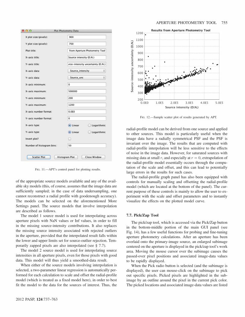
of the appropriate source models available and any of the avail-able sky models (this, of course, assumes that the image data aresufficiently sampled; in the case of data undersampling, onecannot reconstruct a radial profile with goodenough accuracy).The models can be selected on the aforementioned MoreSettings panel. The source models that involve interpolationare described as follows.

The model 1 source model is used for interpolating acrossaperture pixels with NaN values or Inf values, in order to fillin the missing source-intensity contributions. It also replacesthe missing source intensity associated with rejected outliersin the aperture, provided that the interpolated result falls withinthe lower and upper limits set for source-outlier rejection. Tem-porarily zapped pixels are also interpolated (see § 7.7).

The model 2 source model is used for interpolating sourceintensities in all aperture pixels, even for those pixels with gooddata. This model will thus yield a smoothed-data result.

When either of the source models involving interpolation isselected, a two-parameter linear regression is automatically per-formed for each calculation to scale and offset the radial-profilemodel (which is treated as a fixed model here), in order to bestfit the model to the data for the sources of interest. Thus, the

radial-profile model can be derived from one source and appliedto other sources. This model is particularly useful when theimage data have a radially symmetrical PSF and the PSF isinvariant over the image. The results that are computed withradial-profile interpolation will be less sensitive to the effectsof noise in the image data. However, for saturated sources withmissing data at small r, and especially at r ¼ 0, extrapolation ofthe radial-profile model essentially occurs through the compu-tation of the scale and offset, and this can lead to potentiallylarge errors in the results for such cases.

The radial-profile graph panel has also been equipped withcontrols for manually scaling and offsetting the radial-profilemodel (which are located at the bottom of the panel). The cur-rent purpose of these controls is mainly to allow the user to ex-periment with the scale and offset parameters and to instantlyvisualize the effects on the plotted model curve.

7.7. Pick/Zap Tool

The pick/zap tool, which is accessed via the Pick/Zap buttonin the bottom-middle portion of the main GUI panel (seeFig. 14), has a few useful functions for probing and fine-tuningaperture photometry calculations. After an aperture has beenoverlaid onto the primary-image source, an enlarged subimagecentered on the aperture is displayed in the pick/zap tool’s workarea. Moving the mouse cursor over the subimage causes thepassed-over pixel positions and associated image-data valuesto be rapidly displayed.

When the Pick radio button is selected (and the subimage isdisplayed), the user can mouse-click on the subimage to pickout specific pixels. Picked pixels are highlighted in the sub-image by an outline around the pixel in the current pick color.The picked locations and associated image-data values are listed

FIG. 12.—Sample scatter plot of results generated by APT.

FIG. 11.—APT’s control panel for plotting results.

APERTURE PHOTOMETRY TOOL 755

2012 PASP, 124:737–763

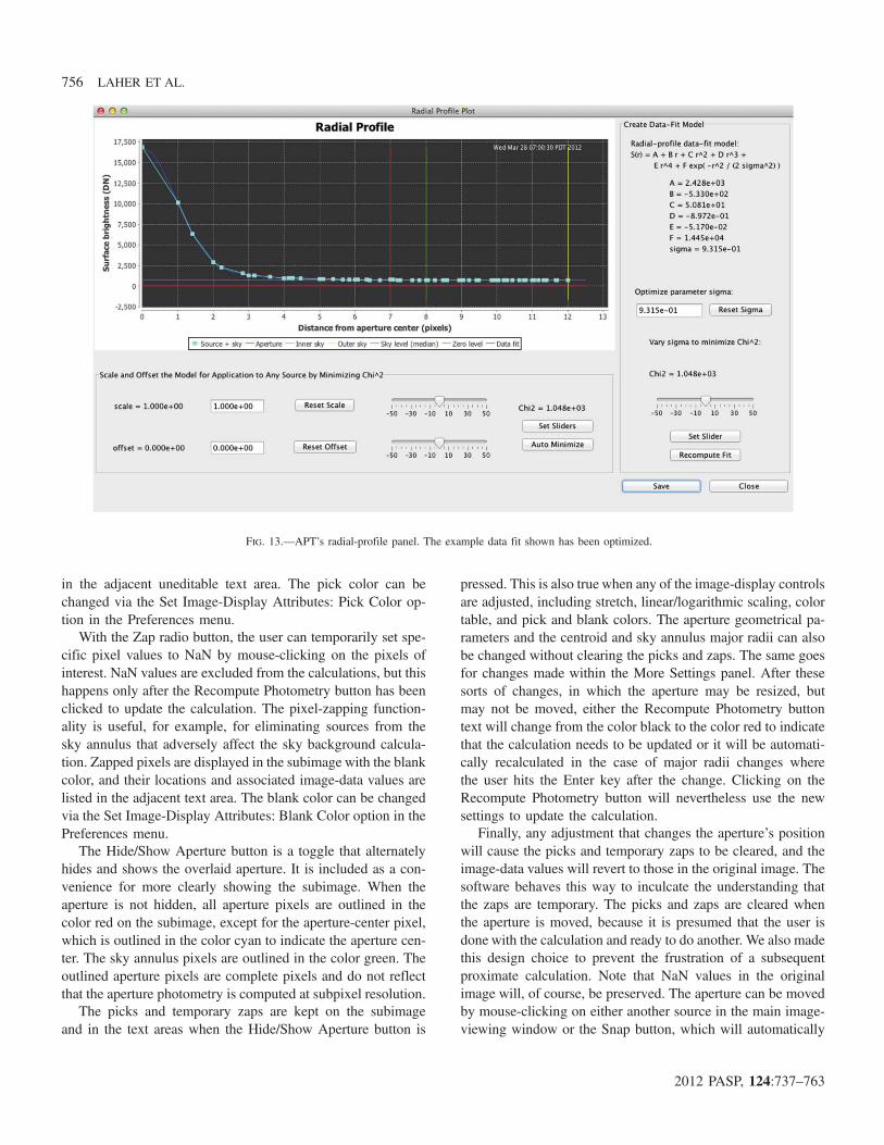
in the adjacent uneditable text area. The pick color can bechanged via the Set Image-Display Attributes: Pick Color op-tion in the Preferences menu.

With the Zap radio button, the user can temporarily set spe-cific pixel values to NaN by mouse-clicking on the pixels ofinterest. NaN values are excluded from the calculations, but thishappens only after the Recompute Photometry button has beenclicked to update the calculation. The pixel-zapping function-ality is useful, for example, for eliminating sources from thesky annulus that adversely affect the sky background calcula-tion. Zapped pixels are displayed in the subimage with the blankcolor, and their locations and associated image-data values arelisted in the adjacent text area. The blank color can be changedvia the Set Image-Display Attributes: Blank Color option in thePreferences menu.

The Hide/Show Aperture button is a toggle that alternatelyhides and shows the overlaid aperture. It is included as a con-venience for more clearly showing the subimage. When theaperture is not hidden, all aperture pixels are outlined in thecolor red on the subimage, except for the aperture-center pixel,which is outlined in the color cyan to indicate the aperture cen-ter. The sky annulus pixels are outlined in the color green. Theoutlined aperture pixels are complete pixels and do not reflectthat the aperture photometry is computed at subpixel resolution.

The picks and temporary zaps are kept on the subimageand in the text areas when the Hide/Show Aperture button is

pressed. This is also true when any of the image-display controlsare adjusted, including stretch, linear/logarithmic scaling, colortable, and pick and blank colors. The aperture geometrical pa-rameters and the centroid and sky annulus major radii can alsobe changed without clearing the picks and zaps. The same goesfor changes made within the More Settings panel. After thesesorts of changes, in which the aperture may be resized, butmay not be moved, either the Recompute Photometry buttontext will change from the color black to the color red to indicatethat the calculation needs to be updated or it will be automati-cally recalculated in the case of major radii changes wherethe user hits the Enter key after the change. Clicking on theRecompute Photometry button will nevertheless use the newsettings to update the calculation.

Finally, any adjustment that changes the aperture’s positionwill cause the picks and temporary zaps to be cleared, and theimage-data values will revert to those in the original image. Thesoftware behaves this way to inculcate the understanding thatthe zaps are temporary. The picks and zaps are cleared whenthe aperture is moved, because it is presumed that the user isdone with the calculation and ready to do another. We also madethis design choice to prevent the frustration of a subsequentproximate calculation. Note that NaN values in the originalimage will, of course, be preserved. The aperture can be movedby mouse-clicking on either another source in the main image-viewing window or the Snap button, which will automatically

FIG. 13.—APT’s radial-profile panel. The example data fit shown has been optimized.

756 LAHER ET AL.

2012 PASP, 124:737–763

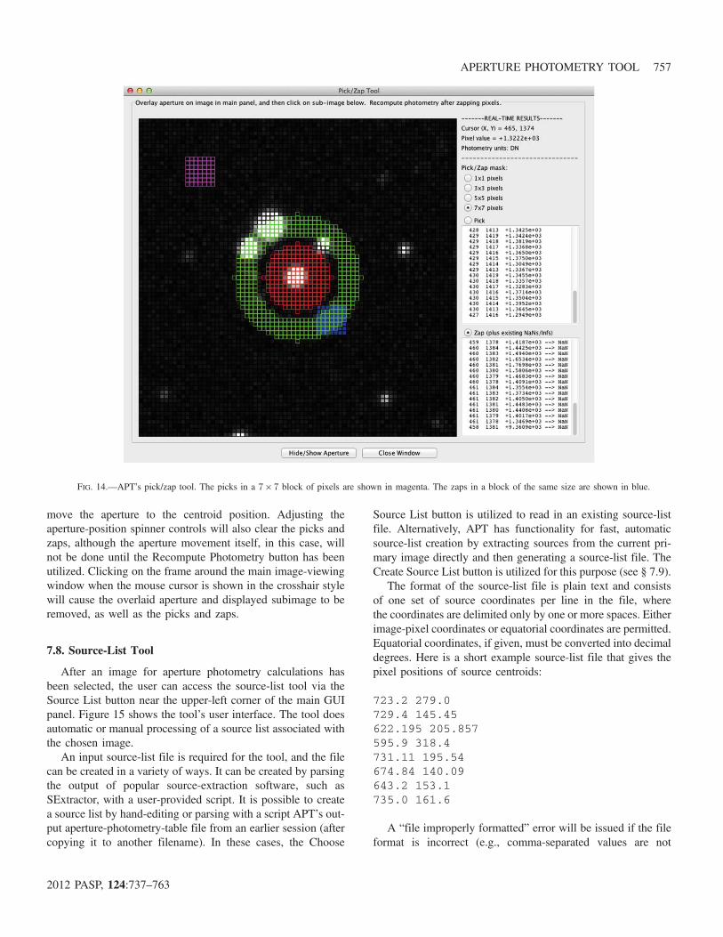
move the aperture to the centroid position. Adjusting theaperture-position spinner controls will also clear the picks andzaps, although the aperture movement itself, in this case, willnot be done until the Recompute Photometry button has beenutilized. Clicking on the frame around the main image-viewingwindow when the mouse cursor is shown in the crosshair stylewill cause the overlaid aperture and displayed subimage to beremoved, as well as the picks and zaps.

7.8. Source-List Tool

After an image for aperture photometry calculations hasbeen selected, the user can access the source-list tool via theSource List button near the upper-left corner of the main GUIpanel. Figure 15 shows the tool’s user interface. The tool doesautomatic or manual processing of a source list associated withthe chosen image.

An input source-list file is required for the tool, and the filecan be created in a variety of ways. It can be created by parsingthe output of popular source-extraction software, such asSExtractor, with a user-provided script. It is possible to createa source list by hand-editing or parsing with a script APT’s out-put aperture-photometry-table file from an earlier session (aftercopying it to another filename). In these cases, the Choose

Source List button is utilized to read in an existing source-listfile. Alternatively, APT has functionality for fast, automaticsource-list creation by extracting sources from the current pri-mary image directly and then generating a source-list file. TheCreate Source List button is utilized for this purpose (see § 7.9).

The format of the source-list file is plain text and consistsof one set of source coordinates per line in the file, wherethe coordinates are delimited only by one or more spaces. Eitherimage-pixel coordinates or equatorial coordinates are permitted.Equatorial coordinates, if given, must be converted into decimaldegrees. Here is a short example source-list file that gives thepixel positions of source centroids:

723.2 279.0729.4 145.45622.195 205.857595.9 318.4731.11 195.54674.84 140.09643.2 153.1735.0 161.6

A “file improperly formatted” error will be issued if the fileformat is incorrect (e.g., comma-separated values are not

FIG. 14.—APT’s pick/zap tool. The picks in a 7 × 7 block of pixels are shown in magenta. The zaps in a block of the same size are shown in blue.

APERTURE PHOTOMETRY TOOL 757

2012 PASP, 124:737–763

allowed). The maximum number of sources per source-list fileallowed by APT is 100,000. A set of radio buttons for the user toindicate the source-list-coordinates type is available on thesource-list-tool panel.

The user has the option of selecting the button labeled Auto-matically Process Source List, in which case calculations will beperformed for all sources in the source list for the current aper-ture photometry settings. Thus, it is important that the userselect the desired settings before mouse-clicking on this button.Once this option has been selected, identical calculations will bedone for all sources in the source list, and a record will be auto-matically saved for each source in the aperture-photometry-table file. The marker Automatic Source-List Processing… willbe written to the aperture-photometry-table file prior to savingthe aperture-photometry records.

Another option available to the user is the Manually ProcessSource List button, in which case an aperture will be overlaidonto the image for the first source in the source list, and themessage “Ready to process source number 1” will be displayed.The user can, at this time, manually adjust any or all of the aper-ture photometry settings for that particular source on the mainGUI panel and via the More Settings button and then press theRecompute Photometry button and view the graphs to makesure that the settings are just right. After the user is satisfied

with the settings for that particular source, the Step ThroughSource List button can be pressed, which will redo the calcula-tion, save a record of the results to the aperture-photometry-table file, and then overlay an aperture onto the image for thenext source in the source list. The marker Manual Source-ListProcessing … will be written to the file prior to saving theresults record for the first source. The above steps are repeatedfor each successive source in the source list. After the source listhas been exhausted, the message “Donewith source list.”will bedisplayed. To reset manual processing and start again (perhapsafter another selection of aperture photometry settings havebeen made), simply press the Manually Process Source List but-ton once more.

7.9. Source-List Generation

The Create Source List button on the source-list-tool panelpops up another panel with functionality to generate a source listby extracting sources from the current primary image (seeFig. 16) and to then write the source list to a file. The sourcelist is generated with image-pixel coordinates. Users can eithersave the source list to the disk location and filename of theirchoice using the Reset Source-List Filename button on the

FIG. 15.—APT’s source-list tool for performing aperture photometry calculations from a source list.

758 LAHER ET AL.

2012 PASP, 124:737–763

panel, or they can keep the default location and filename(see § 7.3).

There are three options for controlling the source-list genera-tion. The Source-List Creation Tool panel has text fields for threeinput parameters: source-detection threshold and minimum andmaximum numbers of contiguous pixels allowed for a source.The source-detection threshold is specified in number of data-distribution half-widths. It is used to calculate the image-datathreshold at each image pixel position. The image-data thresholdis defined as the local background median plus the source-detection threshold times the global dispersion of the image data.The dispersion is computed by taking one-half of the differencebetween the 84 and 16 percentiles. The two remainingparameters control the size range the user allows for detectedsources. The source minimum number of pixels is a parameterused to exclude sources with an insufficient number of detectedpixels above the image-data threshold. The parameter for thesource maximum number of pixels is useful for excluding verylarge sources that may lie outside of the user’s sphere of interest.A source-detection threshold of at least 1.0 is recommended.Either setting the threshold too low or not narrowing the sourcesize range enough may result in more detections than the soft-ware can handle, in which case the software will warn the userand recommend another try with a higher threshold. Up to100,000 segmented detections are currently allowed by the soft-ware, where the segments consist of 100 pixels each.

The algorithm for computing the local background medianis given as follows. The primary image is divided up into

N ×N pixel cells, where N is an odd number that varies withthe size of the image, is chosen to have at least 10 cells acrossthe shortest image dimension, and is allowed to be no smallerthan 33 pixels. The median of the image data in each cell iscomputed, and bilinear interpolation over the cells is then usedto estimate the spatially varying local background median. Spe-cial handling of the calculation is done at the far image edges toavoid extrapolation.

Source detections occur for image-data pixels that are bothgreater than or equal to the spatially varying image-data thresh-old and greater than zero. A source is defined by a set of con-tiguous detections, where contiguous pixels are joined either atpixel sides or corners. The centroid of each source defines itsposition in the image, and the centroid image coordinates arewritten to the specified source-list file.

7.10. Simple-Photometric-Calibration Tool

The software includes a user-friendly tool to provide thecapability of performing simple photometric calibration (seeFig. 17). The tool matches two source lists and computes a singleparameter, the photometric zero point, via sum-of-squared-errorminimization. At least one match is required, but no more than100,000 matches are allowed in the computation. The algorithmmakes two passes through the data. The first pass computes ro-bust data statistics: namely, the median and the data dispersiongiven by one-half of the difference between the 84.1 and 15.9percentiles. The second pass applies outlier rejection andfaint-source rejection to filter the data. A sufficient variety of

FIG. 16.—APT’s source-list creation tool.

APERTURE PHOTOMETRY TOOL 759

2012 PASP, 124:737–763

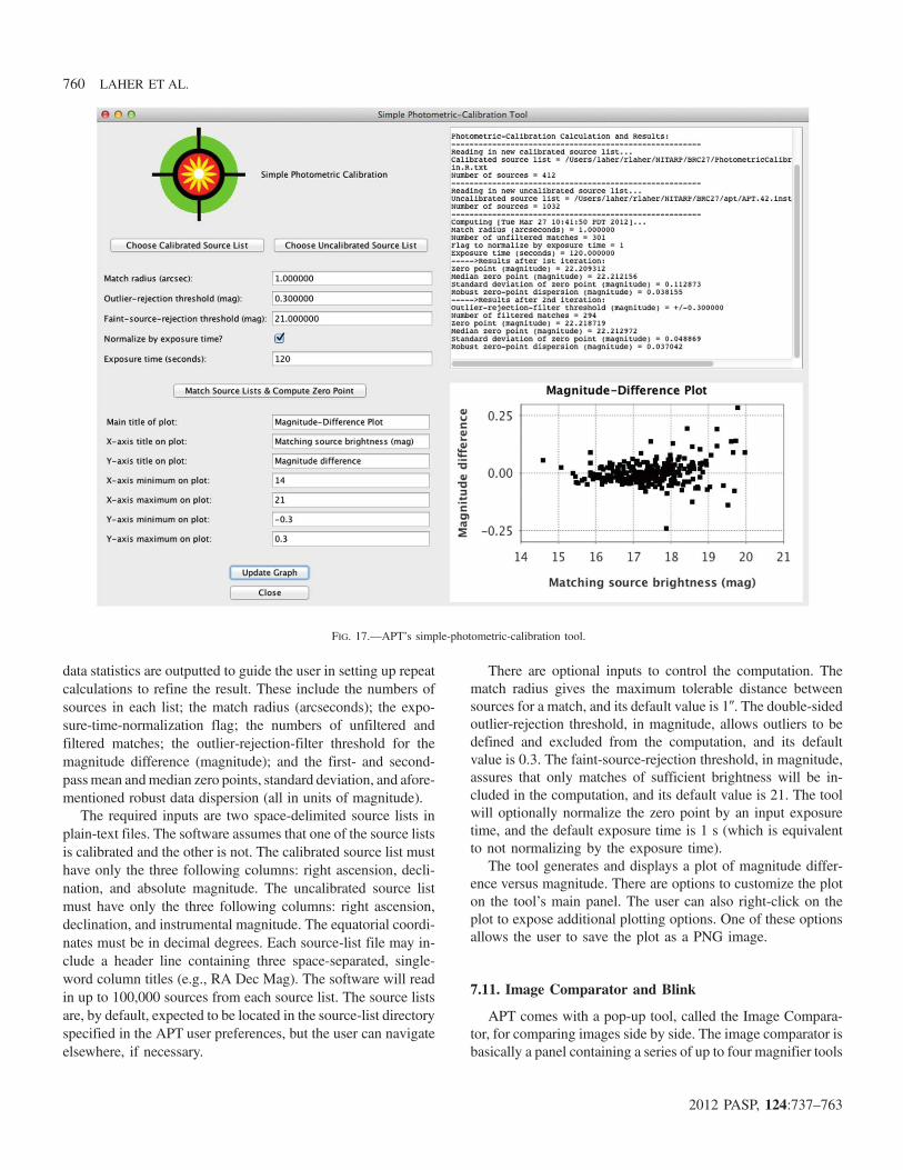
data statistics are outputted to guide the user in setting up repeatcalculations to refine the result. These include the numbers ofsources in each list; the match radius (arcseconds); the expo-sure-time-normalization flag; the numbers of unfiltered andfiltered matches; the outlier-rejection-filter threshold for themagnitude difference (magnitude); and the first- and second-passmean andmedian zero points, standard deviation, and afore-mentioned robust data dispersion (all in units of magnitude).

The required inputs are two space-delimited source lists inplain-text files. The software assumes that one of the source listsis calibrated and the other is not. The calibrated source list musthave only the three following columns: right ascension, decli-nation, and absolute magnitude. The uncalibrated source listmust have only the three following columns: right ascension,declination, and instrumental magnitude. The equatorial coordi-nates must be in decimal degrees. Each source-list file may in-clude a header line containing three space-separated, single-word column titles (e.g., RA Dec Mag). The software will readin up to 100,000 sources from each source list. The source listsare, by default, expected to be located in the source-list directoryspecified in the APT user preferences, but the user can navigateelsewhere, if necessary.

There are optional inputs to control the computation. Thematch radius gives the maximum tolerable distance betweensources for a match, and its default value is 1′′. The double-sidedoutlier-rejection threshold, in magnitude, allows outliers to bedefined and excluded from the computation, and its defaultvalue is 0.3. The faint-source-rejection threshold, in magnitude,assures that only matches of sufficient brightness will be in-cluded in the computation, and its default value is 21. The toolwill optionally normalize the zero point by an input exposuretime, and the default exposure time is 1 s (which is equivalentto not normalizing by the exposure time).

The tool generates and displays a plot of magnitude differ-ence versus magnitude. There are options to customize the ploton the tool’s main panel. The user can also right-click on theplot to expose additional plotting options. One of these optionsallows the user to save the plot as a PNG image.

7.11. Image Comparator and Blink

APT comes with a pop-up tool, called the Image Compara-tor, for comparing images side by side. The image comparator isbasically a panel containing a series of up to four magnifier tools

FIG. 17.—APT’s simple-photometric-calibration tool.

760 LAHER ET AL.

2012 PASP, 124:737–763

that enable simultaneous comparison of the primary imagewith up to three different comparator images (see Fig. 18). Thisfunctionality is accessed via the Image Comparator buttonlocated in the upper-middle portion of the main GUI panel.The comparator images can be offset in x and y relative to theprimary image using the available spinner adjustments, if neces-sary. Separate control over the stretch of each comparator imageis currently not implemented. For comparing images with dras-tically different stretches, judicious use of the primary-imagelogarithmic-stretch capability can compensate somewhat forthis tool’s deficiency.

Closely related to the functionality of the Image Comparatoris APT’s image blink capability. Repeatedly mouse-clicking onthe Blink button located in the lower-middle portion of the mainGUI panel will quickly cycle the image display from the pri-mary image to the first comparator image in the sequence, sub-sequently advancing to the next comparator image, if available,and then eventually back again to the primary image. This capa-bility is good for spotting image pixels with variable stars oraffected by cosmic rays.

7.12. Batch Mode

There are two different options available for running APT inbatch mode. The first is that APT can be executed with an imagespecified on the command line, in which case that image will beloaded and displayed in the GUI:

APT.csh image.fits

The second option is that APT can be executed with both animage and source list specified on the command line, in whichcase the image and source list will be loaded by the software and

processed by APT’s source-list tool, without displayingthe GUI:

APT.csh image.fits source.lst

This noninteractive batch-mode command is handy for gen-erating an aperture-photometry-table file for the source list froma script. Control is returned to the user’s command shell afterAPT terminates. The image file must be specified before thesource-list file. The parameters that control how the source listis processed by the source-list tool are specified by runningAPT beforehand and saving the parameters as user preferencesin the default location (which is loaded automatically upon APTstartup).

7.13. Internationalization

We implemented a simple workaround for the sticky problemof commas used in place of decimal points on computers insome non-US countries. The APT startup scripts (APT.cshand APT.bat) force English as the user’s language and theUnited States as the user’s geographical region when invokingthe JVM. This is done using the following JVM options:

-Duser.language=en -Duser.region=US

The net effect is to require the American usage for inputfloating-point numbers (e.g., in FITS headers) and to ensurethe same for any output floating-point numbers (e.g., written tothe aperture-photometry-table file), regardless of the languageselected when a computer’s operating system was installed.The workaround was verified for an APT installation on aGerman Windows machine.

FIG. 18.—APT’s Image Comparator showing Spitzer IRAC images in the 3.6, 4.5, 5.8, and 8.0 μm bands. The primary image is on the left.

APERTURE PHOTOMETRY TOOL 761

2012 PASP, 124:737–763

8. SOFTWARE LIMITATIONS

Some of the functionality described above is admittedlynot well integrated into the main functionality, and these areascould use more work. For example, the Simple-Photometric-Calibration Tool could be upgraded to allow APT’s outputaperture photometry table as an input (see § 7.10). Below is alist of items that could or will be addressed in later softwareversions (in no particular order). Future software status andupdates will be posted on the APT World Wide Web site.

1. Handle accompanying image-data masks and uncertaintyimages.

2. Account for sky background variation across the aperturein the calculation.

3. Change the number of standard deviations used in outlierrejection for sky background estimation from a hard-codedvalue into a user-specifiable parameter.

4. Inflate the sky background standard deviation after reject-ing outliers, in order to account for the clipping of the distribu-tion’s tails.

5. Include pixel-to-pixel noise correlations and spatiallyvarying co-add coverage depth in the calculation of source-intensity uncertainties.

6. Implement bit flags to indicate potential problems relatedto the calculation; e.g., source saturation, source located nearedge, source in crowded field, etc.; Cf. SExtractor (Bertin &Arnouts 1996).

7. Upgrade the image comparator to have independentstretch controls and automatic image registration using theimages’ WCS solutions.

8. Add functionality to compute a suite of statistics for agiven column of data in the aperture photometry table.

9. Add zoom-in/out capability for the main image-viewing panel.

10. Add a button that rotates an image so that north is up,based on the WCS in the FITS headers.

11. Add functionality to allow manual override of the cur-rently built-in automatic scaling and offsetting of the radial-profile model when used for interpolation.

12. Add an option to exclude saturated pixels when extract-ing sources from an image.

13. Add a tool that measures distances on the dis-played image.

14. Add basic parameter settings as differentiating labels onthe graphs.

15. Add a new Keep Zaps button and eponymous function-ality for the pick/zap tool.

The default maximum image size is 5000 × 5000 pixels,which has been tested on a computer equipped with 2 Gbytesof random-access memory. The maximum-image-size settingunder the Preferences menu can be increased to accommodatelarger images (assuming the user’s machine has sufficient mem-ory) and, in conjunction with this increase, the user may have to

start up APT with a larger heap-space setting. Currently,java -mx1024M APT is executed in APT.csh, which is theAPT C-shell startup script for UNIX-based platforms, and inAPT.bat, which is the batch file for starting up APT onWindows machines. Mac users running APTas a double-click ap-plication can similarly edit this specification in the Contents/Info.plist subdirectory of the APT package (before installingthe package in the Mac Applications directory).

Finally, some of the Spitzer Science Center Spot/LeopardJava classes for conversion from pixel to celestial coordinateshave been incorporated into APT. However, the user is cau-tioned that only the gnomonic (tangent), orthographic, Carte-sian, and Aitoff (for FITS-viewing only) projections areimplemented. Only equatorial coordinates are computed (noGalactic coordinates). Geometric image distortion, up to theninth polynomial order, is handled by the gnomonic projectiononly for cases where

CTYPE1=‘RA—TAN-SIP’CTYPE2=‘DEC–TAN-SIP’

is specified in the image’s FITS header; see Shupe et al.(2005) for a description of the SIP convention. In the absenceof the -SIP suffix in the CTYPE1 and CTYPE2 settings forthe gnomonic projection, APTwill attempt to read and apply thePV i�j distortion keywords generated by SCAMP for theimage’s astrometrical calibration (Bertin 2006a), which is upto seventh polynomial order, identical to the SExtractor imple-mentation. Other types of projections and geometric-distortionrepresentations in the astrometric calculations may be imple-mented as the need arises.

9. CONCLUSION

In this article, we have introduced important new software tothe astronomical community, called Aperture Photometry Toolor APT, which facilitates the visualization of aperture photome-try in a variety of ways. APT is appropriate, useful, and conve-nient for professional work. It is also playing a vital role ineducating the next generation of astronomers in the UnitedStates and abroad. There are indubitably many reasons that giveAPT a purpose in today’s world, and chief among them are itsgraphical user interface and the critical user feedback it pro-vides, its rich medley of tools, machine independence, easeof installation, and intuitive use. Validation of APT has beendone by comparing several large statistical samples of similarresults from SExtractor and APT, which is documented in acompanion article appearing in this issue of the PASP (Laheret al. 2012). It is expected that APTwill continue to be upgradedover time, both to remove any remaining bugs and to augmentthe software with new functionality and capabilities.

We thank the beta testers. In particular, Tom Jarrett, SeppoLaine, Alberto Crespo-Noriega, Bill Reach, Jeonghee Rho, and

762 LAHER ET AL.

2012 PASP, 124:737–763

Nancy Silbermann made numerous helpful suggestions. IngaSaathoff conducted invaluable beta testing in Germany. Weare also grateful to Xiuqin Wu, Trey Roby, Loi Ly, and BoothHartley for generous expert Java programming help and the use

of some of their Java classes. We also thank BenneW. Holwerdafor his insightful suggestions and manuscript corrections. Aper-ture Photometry Tool’s motto Inviso notitia and logo are copy-right © 2012 by the California Institute of Technology.

REFERENCES

Bertin, E. 2006a, ASP Conf. Ser. 351, Astronomical Data AnalysisSoftware and Systems XV (San Francisco: ASP), 112

———. 2006b, SExtractor User’s Manual, Ver. 2.5 (Paris: IAP)Bertin, E., & Arnouts, S. 1996, A&AS, 117, 393Da Costa, G. S. 1992, ASP Conf. Ser. 23, Astronomical CCD Obser-

ving and Reduction Techniques (San Francisco: ASP), 90Daou, D., Pompea, S., & Thaller, M. 2004, BAAS, 36, 1500Holwerda, B. W., 2005, Source Extractor for Dummies (Baltimore:

STScI)Howell, S. B. 1992, ASP Conf. Ser. 23, Astronomical CCD Observing

and Reduction Techniques (San Francisco: ASP), 105Joye, W. A., & Mandel, E. 2003, ASP Conf. Ser. 295, Astronomical

Data Analysis Software and Systems XII (San Francisco:ASP), 489

Laher, R. R., Rebull, L. M., Gorjian, V., Masci, F. J., Fowler, J. W.,Helou, G., & Kulkarni, S. R., et al. 2012, PASP , 124, 764

Rebull, L. M., Gorjian, V., Squires, G., & Team, NITARP2011, BAAS,43, 248.11

Rebull, L. M., Johnson, C. H., Hoette, V., Kim, J. S., Laine, S., Foster,M., Laher, R., Legassie, M., 2011, AJ, 142, 25

Shupe, D. L., Moshir, M., Li, J., Makovoz, D., Narron, R., & Hook, R.N. 2005, in ASP Conf. Ser. 347, Astronomical Data Analysis Soft-ware and Systems XIV (San Francisco: ASP), 491

Tody, D. 1986, Proc. SPIE, 627, 733———. 1993, in ASP Conf. Ser. 52, Astronomical Data Analysis Soft-

ware and Systems II (San Francisco: ASP), 173Wells, D. C., Greisen, E. W., & Harten, R. H. 1981, A&AS, 44,

363

APERTURE PHOTOMETRY TOOL 763

2012 PASP, 124:737–763